the "greenhouse" effect and climate change 1989.pdf · the "greenhouse" effect...
TRANSCRIPT

THE "GREENHOUSE" EFFECT AND CLIMATE CHANGE
John F. B. Mitchell Meteorological Office, Brackne!l, England
Abstract. The presence of radiatively active gases in the Earth's atmosphere (water vapor, carbon dioxide, and ozone) raises its global mean surface temperature by 30 K, making our planet habitable by life as we know it. There has been an increase in carbon dioxide and other trace
gases since the Industrial Revolution, largely as a result of man's activities, increasing the radiative heating of the troposphere and surface by about 2 W m -2. This heating is likely to be enhanced by resulting changes in water vapor, snow and sea ice, and cloud. The associated equilibrium temperature rise is estimated to be between 1 and 2 K, there being uncertainties in the strength of climate feedbacks, particularly those due to cloud. The large thermal inertia of the oceans will slow the rate of warming, so that the expected temperature rise will be smaller than the equilibrium rise. This increases the uncertainty in the expected warming to date, with estimates ranging from less than 0.5 K to over 1 K. The observed increase of 0.5
K since 1900 is consistent with the lower range of these estimates, but the variability in the observed record is such that one cannot necessarily conclude that the observed temperature change is due to increases in trace gases. The
prediction of changes in temperature over the next 50 years depends on assumptions concerning future changes in trace gas concentrations, the sensitivity of climate, and the effective thermal inertia of the oceans. On the basis of our
current understanding a further warming of at least 1 K seems likely. Numerical models of climate indicate that the changes will not be uniform, nor will they be confined to temperature. The simulated warming is largest in high latitudes in winter and smallest over sea ice in summer, with little seasonal variation in the tropics. Annual mean precipitation and runoff increase in high latitudes, and most simulations indicate a drier land surface in northern
mid-latitudes in summer. The agreement between different models is much better for temperature than for changes in the hydrological cycle. Priorities for future research include developing an improved representation of cloud in numerical models, obtaining a better understanding of vertical mixing in the deep ocean, and determining the inherent variability of the ocean-atmosphere system. Progress in these areas should enable detection of a man-made "greenhouse" warming within the next two decades.
1. INTRODUCTION
Our planet is made habitable by the presence of certain gases which trap long-wave radiation emitted from the Earth's surface, giving a global mean temperature of 15øC, as opposed to an estimated-18øC in the absence of an atmosphere. This phenomenon is popularly known as the "greenhouse" effect. By far the most important greenhouse gas is water vapor. However, there is a substantial contribution from carbon dioxide and smaller contributions
from ozone, methane, and nitrous oxide. The concentrations of carbon dioxide, methane, and
nitrous oxide are all known to be increasing, and in recent years, other greenhouse gases, principally chlorofluorocar- bons (CFCs), have been added in significant quantifies to the atmosphere. There are many uncertainties in deducing the consequential climatic effects. Typically, it is esti- mated that increased concentrations of these gases since 1860 may have raised global mean surface temperatures by 0.5øC or so, and the projected concentrations could produce a warming of about 1.5øC over the next 40 years.
,..
This paper is not subject to U.S. copyright.
Published in 1989 by the American Geophysical Union.
Numerical climate models indicate that other changes in climate would accompany the increase in globally averaged temperature, with potentially serious effects on many societal and economic activities.
This review attempts to answer several questions. What is the greenhouse effect (section 2)? Which gases are important and why (section 3)? What are the expected changes in the concentration of
greenhouse gases (section 4)? What are the potential climatic effects, and how are
they determined (section 5)? How will the changes in climate evolve (section 6), and
when will we be able to detect them (section 7)? The aim here is to outline the physical basis of the
projected changes in climate due to enhancing the greenhouse effect and to identify the main areas of uncertainty. This review will, therefore, be selective rather than comprehensive. For a more detailed and complete discussion of the greenhouse effect the reader is referred to the major reviews edited by MacCracken and Luther [1985] and Bolin et al. [1986].
Reviews of Geophysics, 27, 1 / February 1989 pages 115-139
Paper number 89RG00094
ß 115 ß
116 . REVIEWS OF GEOPHYSICS / 27,1
2. THE GREENHOUSE EFFECT
2.1. Radiative Effects
The Earth-atmosphere system is heated by solar (short-wave radiation at a mean rate of S O (1 - (z)/4, where S O is the solar "constant," (z is the fraction of radiation reflected by the Earth and atmosphere, and the factor 4 allows for the spherical geometry of the Earth. This must be balanced by the emission of long-wave (thermal or
,,
infrared) radiation to space (Figure la). The rate of cooling is given by c•T• 4, where c• is Stefan's constant and T• is the effective radiating temperature of the system. At equilibrium
So(1 - (:z)/4 = 6• (1)
which assuming the current albedo of 0.30 gives a value of T e corresponding to 255 K (-18øC). In the absence of an atmosphere, T• will be the Earth's surface temperature.
Solar Longwave
Incoming Reflected
(a) No atmosphere
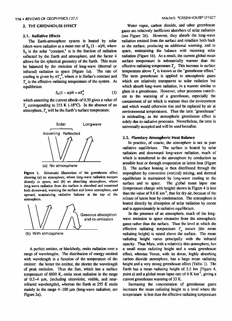
Figure 1. Schematic illustration of the greenhouse effect showing (a) no atmosphere, where long-wave radiation escapes directly to space, and (b) an absorbing atmosphere, where long-wave radiation from the surface is absorbed and reemitted both downward, warming the surface and lower atmosphere, and upward, maintaining radiative balance at the top of the atmosphere.
• • /• •Gaseousabs. or.ption mission
(b) With atmosphere
A perfect emitter, or blackbody, emits radiation over a range of wavelengths. The distribution of energy emitted with wavelength is a function of the temperature of the emitter: the hotter the emitter, the shorter the wavelength of peak emission. Thus the Sun, which has a surface temperature of 6000 K, emits most radiation in the range of 0.2-4 !.tm, (including ultraviolet, visible, and near- infrared wavelengths), whereas the Earth at 255 K emits mainly in the range 4-100 !.tm (long-wave radiation; see Figur e 2a).
Mitchell: "GREENHOUSE" EFFECT
Water vapor, carbon dioxide, and other greenhouse gases are relatively inefficient absorbers of solar radiation (see Figure 2b). However, they absorb the long-wave radiation emitted from the surface and reradiate both back
to the surface, producing an additional warming, and to space, maintaining the balance with incoming solar radiation (Figure lb). As a result, the current global mean surface temperature is substantially warmer than the effective radiating temperature T•. This increase in surface temperature above T• is known as the "greenhouse effect." The term greenhouse is applied to atmospheric gases which are relatively transparent to solar radiation but which absorb long-wave radiation, in a manner similar to glass in a greenhouse. However, other processes contrib- ute to the warming of a greenhouse, especially the containment of air which is warmer than the environment
and which would otherwise rise and be replaced by air at environmental temperatures. Thus the term "greenhouse" is misleading, as the atmospheric greenhouse effect is solely due to radiative processes. Nevertheless, the term is universally accepted and will be used hereafter.
2.2. Planetary Atmospheric Heat Balance In practice, of course, the atmosphere is not in pure
radiative equilibrium. The surface is heated by solar radiation and downward long-wave radiation, much of which is transferred to the atmosphere by conduction as sensible heat or through evaporation as latent heat (Figure 3). The surface heating is then distributed through the troposphere by convective (vertical) mixing, and thermal equilibrium is maintained by long-wave cooling to the surface and to space. The global mean lapse rate (temperature change with height) shown in Figure 4 is less than the value of 9.6 K km '•, that for dry air, because of the release of latent heat by condensation. The stratosphere is heated direcfiy by absorption of solar radiation by ozone and is approximately in radiative equilibrium.
In the presence of an atmosphere, much of the long- wave emission to space emanates from the atmospheric gases rather than the surface. Thus the level at which the effective radiating temperature T• occurs (the mean radiating height) is raised above the surface. The mean radiating height varies principally with the infrared opacity. Thus Mars, with a relatively thin atmosphere, has a small mean radiating height and a weak greenhouse effect, whereas Venus, with its dense, highly absorbing carbon dioxide atmosphere, has a large mean radiating height and a very strong greenhouse effect (Table 1). The Earth has a mean radiating height of 5.5 km (Figure 4, point a) and a global mean lapse rate of 6 K km 4, giving a current greenhouse warming of 33 K.
Increasing the concentration of greenhouse gases increases the mean radiating height to a level where the temperature is less than the effective radiating temperature

Mitchell: "GREENHOUSE" EFFECT 27,1 / REVIEWS OF GEOPHYSICS ß 117
uJ
Black Body /,,--%
Curve • A
Wave number (cm -•)
50000 10000 5000 2000 1428 1000 663 333 200 100
0.1 0.15 0.2 0.3 0.5 1.0 1.5 2 3 5 10 15 20 30 50 100
Wavelength pm
100
80-
40-
20-
o
o
Ground
Level
I I I 1 02 02 02 03
Figure 2. (a) Spectral distribution of long-wave emission from blackbodies at 6000 K and 255 K, corresponding to the mean emitting temperatures of the Sun and Earth, respectively, and (b) percentage of atmospheric absorption for radiation passing from
H20 (Rotation)
B
IJUll L J I I II c;,i Iii • • illill I I .oJL o I.o I o, II L'! .o // H20 ,.• I I N20 I Ii co,
co OH4 4 CF2CI2
the top of the atmosphere to the surface. Notice the compara- tively weak absorption of the solar spectrum and the region of weak absorption from 8 to 12 !xm in the long-wave spectrum [from MacCracken and Luther, 1985].
SPACE INCOMING SOLAR OUTGOING RADIATION
R ADI ATI ON Shortwave Longwave
100 8 17 6 9 40 20
ATMO .HR [• / / / " t t S \X•Backscattered/ / / %••y?ir // Net Emission • by
Emission
Absorbed by • \ X •' /• Water Vapor, ' ' Water Vapor 19 \ x / , CO 2 O3 by Clouds ' • Reflected / '
Water Vapor, • • 106 CO2'O3 • La•ent
A s • r • Heat Flux b orbed by • Reflected Clouds • by Surface Sensible
• Heat Flux Absorbed LONGWAVE RADIATION • 46 115 100 7 24
OCEAN, LAND
Figure 3. Schematic representation of the atmospheric heat balance. The units are percent of incoming solar radiation. The solar fluxes are shown on the left-hand side, and the longwave
(thermal IR) fluxes are on the right-hand side [from MacCracken and Luther, 1985].

1111 ß REVIEWS OF GEOPHYSICS / 27,1 Mitchell' "GREENHOUSE" EFFECT
T,. In order to maintain the radiation balance of the Earth-atmosphere system (equation (1)), the troposphere and surface must warm until the temperature at the new mean radiating height is equal to T, (Figure 4, point c). The surface warming may be modified by accompanying changes in albedo or lapse rate, as discussed in section 5.
12
10
(
Enhanced
•--•'k• Present I'- Mean radiating
heights
/ I I '• I 3oo
255 288
STRATOSPHERE
TROPOSPHERE
SURFACE
Temperature (K)
Figure 4. Effect of increasing CO 2 on the vertical profile of temperature (schematic). Enhancing CO 2 raises the mean radiating height as shown. The temperature profile warms until the temperature at the new mean radiating height reaches 255 K, the current effective radiating temperature of the Earth.
An important point to note is that the surface and troposphere are strongly coupled: if the troposphere warms, the surface must warm also and vice versa. Much
of the surface warming due to greenhouse gases arises from direct radiative heating of the troposphere [see Lal and Ramanathan, 1984]. In order to include the change in radiative heating at the surface and in the troposphere the term "greenhouse heating" used in this paper refers to the change in the net downward radiative flux at the tropospause.
3. WHICH GASES ARE CLIMATICALLY
IMPORTANT, AND WHY?
The contribution of a gas to the greenhouse effect depends on the wavelength at which the gas absorbs radiation, the concentration of the gas, the strength of absorption per molecule (line strength), and whether or not other gases absorb strongly at the same wavelengths. As a consequence, one molecule of dichlorodifluoromethane
(CFC12) is about 104 times more effective in "trapping" long-wave radiation than one molecule of carbon dioxide in the present atmosphere. The factors governing absorp- tion are discussed in more detail below so that the reader
may understand why some gaes are more important or potentially more important climatically than others.
TABLE 1. Greenhouse Effect on Terrestrial Planets
Planet
Solar Mean Effective Observed Irradiance radiating radiating surface
temper- temper- S O , Wtn '2 Albedo ct level, km ature, K ature, K
Mars
Earth
Venus
589 0.15 1 217 -•220 1367 0.30 5.5 255 288 2613 0.75 70 232 -•700
From National Research Council [ 1982].
3.1. What Determines the Wavelengths of Absorption? Gases absorb and emit radiation at wavelengths which
correspond to transitions between discrete energy levels. The relation between the change in energy level AE and the wavelength 3• of associated radiation is given by
AE = h/2x3•
where h is the Planck constant. Hence each transition is
associated with a discrete wavelength, and larger energy jumps correspond to shorter wavelengths. Diatomic symmetric gases such as oxygen have no permanent dipole moment, so the possible transitions are limited to changes in electronic state which involve large energies and hence short wavelengths (Figure 2b). On the other hand, triatomic molecules such as water and carbon dioxide have
in addition smaller vibrational and rotational energy transitions corresponding to infrared wavelengths. Water vapor absorbs strongly near 6.3 gm and 2.7 gm because of changes in molecular vibrational energy and at wavelengths greater than about 18 gm because of changes in rotational energy (Figure 2b). Carbon dioxide absorbs strongly around 15 gm near the peak of the long-wave spectrum (Figure 2b).
3.2. What Determines the Size of the Contribution to the Greenhouse Effect?
Although each transition is associated with a discrete wavelength, the interval over which absorption occurs is "broadened" by addition or removal of energy due to molecular collisions (pressure broadening) or the Doppler frequency shift due to the random velocities of molecules (Doppler broadening). If absorption is strong, there may be complete absorption (saturation) around the central wavelength of the spectral line (Figure 5).
Both water vapor and carbon dioxide absorb long-wave radiation over a range of frequencies (Figure 2b), and the relatively high concentration of these two gases (Table 2) ensures that many of the spectral lines are saturated. Any increase in the absorption due to enhancing the concentra- tion of these gases is limited to the wings of the absorption lines (Figure 5). Consequently, the radiative heating due to these gases increases logarithmically, not linearly, with
Mitchell' "GREENHOUSE" EFFECT 27,1 / REVIEWS OF GEOPHYSICS ß 119
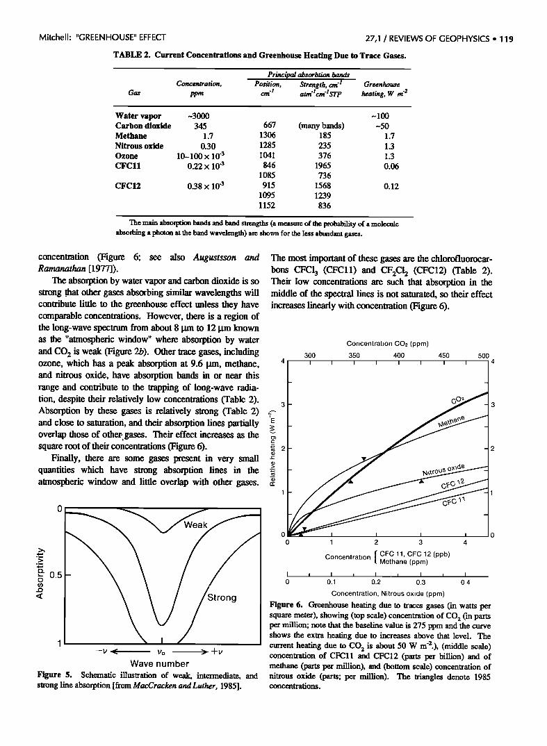
TABLE 2. Current Concentrations and Greenhouse Heating Due to Trace Gases.
Principal absorbtion bands Concentration, Position, Strength, cm '! Greenhouse
Gas ppm cm '• atm '• cm '• STP heating, W m '2
Water vapor -3000 ~100 Carbon dioxide 345 667 (many bands) ~50 Methane 1.7 1306 185 1.7 Nitrous oxide 0.30 1285 235 1.3 Ozone 10-100 x 10 '3 1041 376 1.3 CFCll 0.22 x 10 '3 846 1965 0.06
1085 736
CFC12 0.38 x 10 '3 915 1568 0.12 1095 1239 1152 836
The main absorption bands and band strengths (a measure of the probability of a molecule absorbing a photon at the band wavelength) are shown for the less abundant gases.
concentration (Figure 6; see also Augustsson and Ramanathan [1977]).
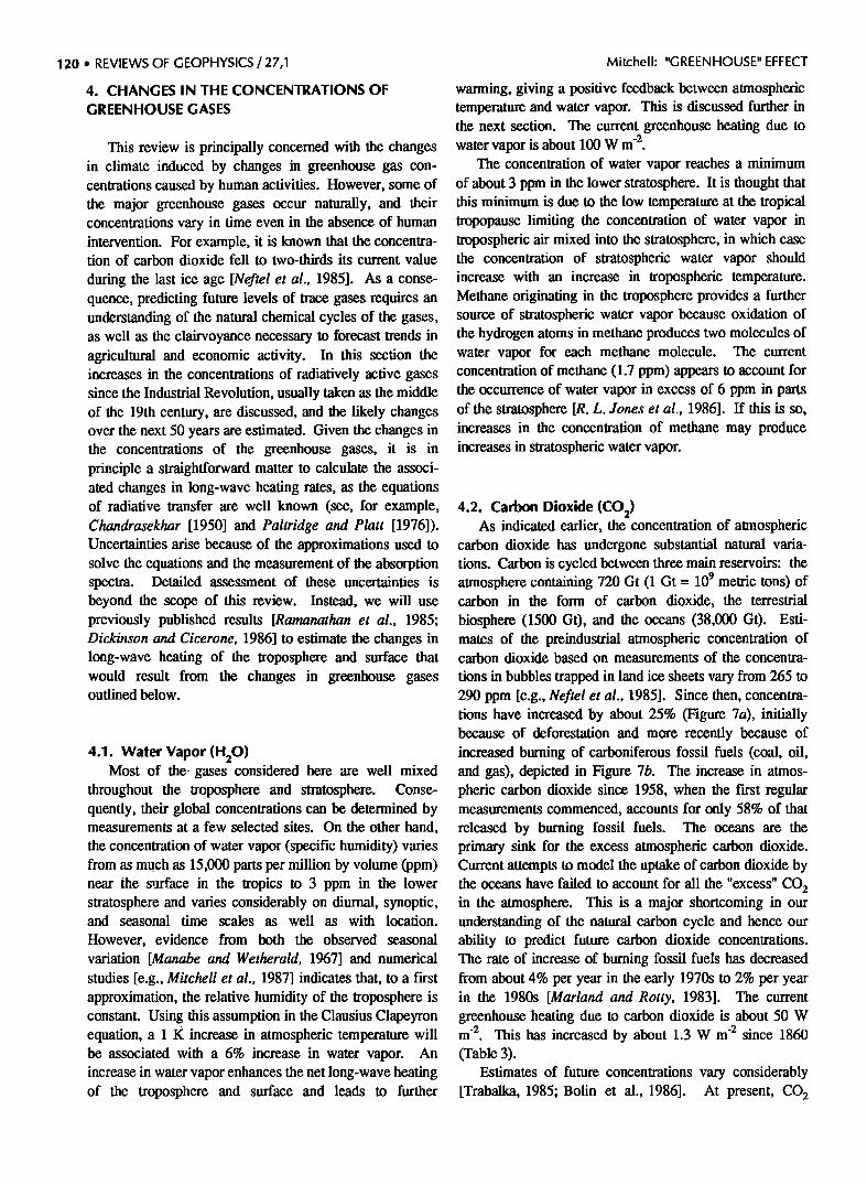
The absorption by water vapor and carbon dioxide is so strong .that other gases absorbing similar wavelengths will contribute little to the greenhouse effect unless they have comparable concentrations. However, there is a region of the long-wave spectrum from about 8 !xm to 12 gm known as the "atmospheric window" where absorption by water and CO 2 is weak (Figure 2b). Other trace gases, including ozone, which has a peak absorption at 9.6 !xm, methane, and nitrous oxide, have absorption bands in or near this range and contribute to the trapping of long-wave radia-
tion, despite their relatively low concentrations (Table 2). Absorption by these gases is relatively strong (Table 2) and close to saturation, and their absorption lines partially overlap those of other;gases. Their effect increases as the square root of their concentrations (Figure 6).
Finally, there are some gases present in very small quantifies which have strong absorption lines in the atmospheric window and little overlap with other gases.
1
Wave number
Figure 5. Schematic illustration of weak, intermediate, and strong line absorption [from MacCracken and Luther, 1985].
The most important of these gases are the chlorofluorocar- bons CFC1 a (CFCll) and CF2C12 (CFC12) (Table 2). Their low concentrations are such that absorption in the middle of the spectral lines is not saturated, so their effect increases linearly with concentration (Figure 6).
Concentration C02 (ppm)
300 350 400 450 500 4
I I I I I I I I I
I I I I
0 1 2 3 4
Concentration [ CFC 11, CFC 12 (ppb) Methane (ppm)
I [ I I I I I [ I 0 0.1 0.2 0.3 0.4
Concentration, Nitrous oxide (ppm)
Figure 6. Greenhouse heating due to traces gases (in watts per square meter), showing (top scale) concentration of CO 2 (in parts per million; note that the baseline value is 275 ppm and the curve shows the extra heating due to increases above that level. The current heating due to CO 2 is about 50 W m'2.), (middle scale) concentration of CFCll and CFC12 (parts per billion) and of methane (parts per million), and (bottom scale) concentration of nitrous oxide (parts; per million). The triangles denote 1985 concentrations.
120 ø REVIEWS OF GEOPHYSICS / 27,1
4. CHANGES IN THE CONCENTRATIONS OF
GREENHOUSE GASES
This review is principally concerned with the changes in climate induced by changes in greenhouse gas con- centrations caused by human activities. However, some of the major greenhouse gases occur naturally, and their concentrations vary in time even in the absence of human intervention. For example, it is known that the concentra- tion of carbon dioxide fell to two-thirds its current value
during the last ice age [Neftel et al., 1985]. As a conse- quence, predicting future levels of trace gases requires an understanding of the natural chemical cycles of the gases, as well as the clairvoyance necessary to forecast trends in agricultural and economic activity. In this section the increases in the concentrations of radiatively active gases since the Industrial Revolution, usually taken as the middle of the 19th century, are discussed, and the likely changes over the next 50 years are estimated. Given the changes in the concentrations of the greenhouse gases, it is in principle a straightforward matter to calculate the associ- ated changes in long-wave heating rates, as the equations .of radiative transfer are well known (see, for example, Chandrasekhar [1950] and Paltridge and Platt [1976]). Uncertainties arise because of the approximations used to solve the equations and the measurement of the absorption spectra. Detailed assessment of these uncertainties is beyond the scope of this review. Instead, we will use previously published results [Ramanathan et al., 1985; Dickinson and Cicerone, 1986] to estimate the changes in long-wave heating of the troposphere and surface that would result from the changes in greenhouse gases outlined below.
4.1. Water Vapor (H20) Most of the-gases considered here are well mixed
throughout the troposphere and stratosphere. Conse- quently, their global concentrations can be determined by measurements at a few selected sites. On the other hand,
the concentration of water vapor (specific humidity) varies from as much as 15,000 parts per million by volume (ppm) near the surface in the tropics to 3 ppm in the lower stratosphere and varies considerably on diurnal, synoptic, and seasonal time scales as well as with location.
However, evidence from both the observed seasonal variation [Manabe and Wetheraid, 1967] and numerical
studies [e.g., Mitchell et al., 1987] indicates that, to a first approximation, the relative humidity of the troposphere is constant. Using this assumption in the Clausius Clapeyron equation, a 1 K increase in atmospheric temperature will be associated with a 6% increase in water vapor. An increase in water vapor enhances the net long-wave heating of the troposphere and surface and leads to further
Mitchell: "GREENHOUSE" EFFECT
warming, giving a positive feedback between atmospheric temperature and water vapor. This is discussed further in the next section. The current greenhouse heating due to water vapor is about 100 W m '2.
The concentration of water vapor reaches a minimum of about 3 ppm in the lower stratosphere. It is thought that this minimum is due to the low temperature at the tropical tropopause limiting the concentration of water vapor in tropospheric air mixed into the stratosphere, in which case the concentration of stratospheric water vapor should increase with an increase in tropospheric temperature. Methane originating in the troposphere provides a further source of stratospheric water vapor because oxidation of the hydrogen atoms in methane produces two molecules of water vapor for each methane molecule. The current concentration of methane (1.7 ppm) appears to account for the occurrence of water vapor in excess of 6 ppm in parts of the stratosphere [R. L. Jones et al., 1986]. If this is so, increases in the concentration of methane may produce increases in stratospheric water vapor.
4.2. Carbon Dioxide (CO:) As indicated earlier, the concentration of atmospheric
carbon dioxide has undergone substantial natural varia- tions. Carbon is cycled between three main reservoirs: the atmosphere containing 720 Gt (1 Gt = 109 metric tons) of carbon in the form of carbon dioxide, the terrestrial
biosphere (1500 Gt), and the oceans (38,000 GO. Esti- mates of the preindustrial atmospheric concentration of carbon dioxide based on measurements of the concentra-
tions in bubbles trapped in land ice sheets vary from 265 to 290 ppm [e.g., Neftel et al., 1985]. Since then, concentra- tions have increased by about 25% (Figure 7a), initially because of deforestation and more recently because of increased burning of carboniferous fossil fuels (coal, oil, and gas), depicted in Figure 7b. The increase in atmos- pheric carbon dioxide since 1958, when the first regular measurements commenced, accounts for only 58% of that released by burning fossil fuels. The oceans are the primary sink for the excess atmospheric carbon dioxide. Current attempts to model the uptake of carbon dioxide by the oceans have failed to account for all the "excess" CO2 in the atmosphere. This is a major shortcoming in our understanding of the natural carbon cycle and hence our ability to predict future carbon dioxide concentrations. The rate of increase of burning fossil fuels has decreased from about 4% per year in the early 1970s to 2% per year in the 1980s [Marland and Rotty, 1983]. The current greenhouse heating due to carbon dioxide is about 50 W m '•. This has increased by about 1.3 W m '• since 1860 (Table 3).
Estimates of future concentrations vary considerably [Trabalka, 1985; Bolin et al., 1986]. At present, CO:

Mitchell' "GREENHOUSE" EFFECT 27,1 / REVIEWS OF GEOPHYSICS ß 1:21
TABLE 3. Past and Projected Greenhouse Gas Concentrations and Associated Changes in Greenhouse Heating AQ
Gas
Assumed 1860 AQ Estimated 2035 Estimated AQ Concentration 1860-1985, Concentration 1985-2035,
ppm W m '2 ppm W m '2
Carbon dioxide 275. 1.3 475 1.8 Methane 1.1 0.4 2.8 0.5 Nitrous oxide 0.28 0.05 0.38 0.15 CFCll 0 0.06 1.6 x 10 's 0.35 CFC12 0 0.12 2.8 x 10 's 0.69
Total 1.9 3.5
350
•- 340 ._(2
(• 330
o
d 320
310 -- ,,I,,,,1•, ,, I• •1• •1• ,• •1•,•
1960 1965 1970 1975 1980 1985 (a) Year
Figure 7. (a) Concentration of atmospheric carbon dioxide in parts per million (ppm) of dry air versus time in years observed with a continuously recording nondispersive infrared gas analyzed at Mauna Loa Observatory, Hawaii [from Keeling et al., 1988] and (b) fossil fuel CO 2 emissions: 1860-1982 [Marland and Rotty, 1983] (reproduced by Trabalka [1985]).
.-. 6
1860
(b)
ß
1880 1900 1920 1940 1960
Year
1980
concentrations are increasing at a rate of 1.5 ppm (equivalent to 0.48%) per year, which, if maintained, would give a concentration of 420 ppm by 2035. Most scenarios assume a gradual increase in emission rates. A growth in emission rates of 1.4% per year assuming 50% of fossil fuel CO 2 remains in the atmosphere (scenario B [Trabalka et al., 1986]) would give a concentration of about 475 ppm by 2035, consistent with that assumed by
Ramanathan et al. [1985] and the median scenario of Nordhaus and Yohe [1983]. This would enhance the
tropospheric/surface heating by a further 1.8 W m '2 (Table 3).
4.3. Methane (CH4) The concentration of methane was about 0.7 ppm 400
years ago [Craig and Chou, 1982] and is now 1.7 ppm, contributing about 1.7 W m '2 to the greenhouse effect, The increase since 1860 alone has added about 0.4 W m '2 (Table 3). Over the last decade, amounts have increased by about 1% per year [Blake and Rowland, 1988]. The main natural sources for atmospheric methane are believed to be paddy fields, ruminants, and wetlands. A recent
analysis of 14½/12½ ratios and 13o12 ½ ratios suggests that about 32% of atmospheric methane originates from fossil fuel burning [Lowe et al., 1988]. The major known sink is photochemical oxidation in the troposphere by the hydroxyl radical OH. As the current methane budget is not accurately known, the prediction of future concentrations is difficult. If the current rate of increase is maintained, concentrations will reach 2.8 ppm in the next 50 years, contributing an additional 0.5 W m '2 in radiative heating.
4.4. Nitrous Oxide (N20) The preindustrial concentration has been estimated to
be 0.28 ppm [Bolin et al., 1986], though lower values have been quoted [Worm Meteorological Organization, 1985]. The increase to the present amount accounts for an extra heating of 0.05 W m '2. The current rate of increase is 0.2% per year [Weiss, 1981], which, if maintained, would produce a concentration of 0.332 ppm in 2035. The sources of tropospheric N20 are believed to include microbial processes in soil and water, nitrogen fertilizers, and fossil fuel and agricultural burning. The main sink is photolysis in the stratosphere with the O(•D) state of atomic oxygen. Given the sketchy nature of our under- standing of the N20 budget, projection of the future concentrations must be regarded as speculative. Ramanathan et al. [1985] assume a 2030 value of 0.375
122 ß REVIEWS OF GEOPHYSICS / 27,1 Mitchell: "GREENHOUSE" EFFECT
ppm on the basis of the simple model used by Weiss [1981]; here we adopt a concentration of 0.38 ppm by 2035, contributing a further 0.15 W m '2 to the greenhouse effect (Table 3).
4.5. Chlorofluoromethanes (CFC11 and CFC12) The atmospheric concentrations of CFC11 and CFC12
can be accounted for by industrial production, allowing for their destruction in the stratosphere and uptake by the oceans. Their current contribution to the greenhouse effect is small (Table 3). If production is maintained at present levels, the concentration of CFC11 and CFC12 will rise to
0.5 and 1.0 parts per billion (ppb) within 40 years and to 0.7 and 2.1 ppb at equilibrium [Dickinson and Cicerone, 1986]. The concentration of these two gases is at present increasing at 5% per year. If this rate of increase is maintained, concentrations will reach 2.7 and 4.6 ppb, consistent with the upper limit used by Ramanathan et al. [ 1985]. In Table 3 a 4% per year increase in concentration is assumed, adding 1.04 W m '2 to the net global heating rate by 2035 (Table 3).
Note that the potential contribution of these two gases is very sensitive to the assumed growth rate. Without an increase in emission rates they could add 0.5 W m '2 to the greenhouse heating rate within the next 50 years. The reductions proposed in the 1987 Montreal Protocol would reduce this to about 0.3 W m '2 [Wigley, 1988].
4.6. Ozone (0 3 ) Tropospheric ozone tends to warm the Earth's surface
through the greenhouse effect, but stratospheric ozone has the opposite effect because of absorption of ultraviolet (short-wave) radiation. There is evidence of a slight decrease in total ozone amounts over the period 1978-1985 due mainly to reductions in the stratosphere [Watson et al., 1988]. About 10% of atmospheric ozone occurs in the troposphere. There are indications of large local increases in ozone at the surface [Bolin et al., 1986], mainly from sites near industrial regions in the northern hemisphere [Volz and Kley, 1988]. The lifetime of ozone molecules in the troposphere is short, and the spatial variations are large, so it is difficult to estimate globally averaged trends. Hence ozone has been omitted from Table 3. Increases in surface ozone alone would have little
greenhouse effect, but a 25% increase through the depth of the troposphere would add 0.2 W m '2 to greenhouse heating.
Many other trace gases were considered by Ramanathan et al. [1985], but their likely contribution is negligible. Methane, nitrous oxide, and ozone undergo chemical cycles which involve other gases (for example, carbon monoxide and peroxyacetyl nitrate) which are also known to be increasing in concentration [Worm Meteorological Organization, 1985; Derwent, 1987].
Since many of the chemical processes are nonlinear, the simple extrapolations used in Table 3 may not be valid. This and other uncertainties, particularly those related to industrial production, should be borne in mind in assessing the values quoted in Table 3.
The estimated increase in long-wave heating of the troposphere and surface since the beginning of the Industrial Revolution is about 1.9 W m '2 (ignoring effects of changes in ozone). A further increase of 3.5 W m '2 seems likely by 2035, though estimates for the next 60 years range from 2.2 W m '2 to 7.2 W m '2 [Dickinson and Cicerone, 1986]. Whereas it is relatively easy to estimate the increase in heating given the changes in greenhouse gas amounts, it less easy to estimate the resulting changes in temperature. This is because the atmosphere adjusts to the perturbed heating rates in ways which may enhance or reduce the magnitude of the response (positive and negative feedbacks), and the thermal inertia of the oceans slows down the rate at which the atmosphere and land surface warm up. Attempts to quantify these two effects are described in the following two sections.
5. DETERMINATION OF THE EQUILIBRIUM CLIMATIC EFFECTS
According to Arrhenius [1896] the possibility that the absorption of long-wave radiation by atmospheric gases would influence ground temperature was recognized by Fourier as early as 1827. Tyndall [1861] attempted to measure the long-wave absorption by atmospheric gases, and Arrhenius [1896] tried to estimate the changes in surface temperatures resulting from the increased con- centrations of "carbonic acid" (carbon dioxide). Arrhenius used data on the atmospheric absorption of moonlight collected by Langley some years earlier. Later studies provided a range of estimates of the surface temperature change due to doubling atmospheric carbon dioxide, with the value arrived at depending very much on the assump- tions made. For example, Plass [1956] considered the surface energy balance assuming radiative equilibrium and a constant atmospheric specific humidity giving a warming of 2.5 K. Moller [1963], on the other hand, assumed that
relative humidity remained constant, adding a strong positive feedback to give a value of 9.6 K. Manabe and Wetheraid [1967] pointed out that the ground and atmos- phere are not in radiative equilibrium (see also Figure 3) and allowed for the convective transfer of heat from the
surface to the atmosphere (using a radiative-convective model), giving a warming of 2.9 K on doubling CO 2. Thus the differences in the earlier results could be attributed to
the different assumptions made in formulating the one-dimensional models used in these studies. There have
been many studies of climate sensitivity using radiative-
Mitchell: "GREENHOUSE" EFFECT 27,1 / REVIEWS OF GEOPHYSICS ß 123
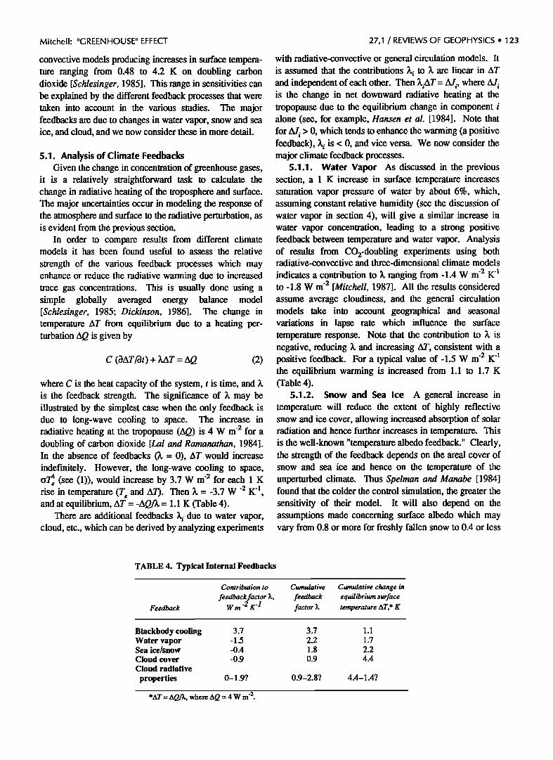
convective models producing increases in surface tempera- ture ranging from 0.48 to 4.2 K on doubling carbon dioxide [Schlesinger, 1985]. This range in sensitivities can be explained by the different feedback processes that were taken into account in the various studies. The major feedbacks are due to changes in water vapor, snow and sea ice, and cloud, and we now consider these in more detail.
5.1. Analysis of Climate Feedbacks Given the change in concentration of greenhouse gases,
it is a relatively straightforward task to calculate the change in radiative heating of the troposphere and surface. The major uncertainties occur in modeling the response of the atmosphere and surface to the radiative perturbation, as is evident from the previous section.
In order to compare results from different climate models it has been found useful to assess the relative
strength of the various feedback processes which may enhance or reduce the radiative warming due to increased trace gas concentrations. This is usually done using a simple globally averaged energy balance model [Schlesinger, 1985; Dickinson, 1986]. The change in temperature AT from equilibrium due to a heating per- turbation AQ is given by
C (3AT/3t) + )•AT = AQ (2)
where C is the heat capacity of the system, t is time, and )• is the feedback strength. The significance of 3, may be illustrated by the simplest case when the only feedback is due to long-wave cooling to space. The increase in radiative heating at the tropopause (AQ) is 4 W m '2 for a doubling of carbon dioxide [Lal and Rarnanathan, 1984]. In the absence of feedbacks (3, = 0), AT would increase indefinitely. However, the long-wave cooling to space, c• (see (1)), would increase by 3.7 W m '2 for each 1 K rise in temperature (T• and AT). Then • = -3.7 W-2 K-•, and at equilibrium, AT = -AQ/3, = 1.1 K (Table 4).
There are additional feedbacks 3, i due to water vapor, cloud, etc., which can be derived by analyzing experiments
with radiative-convective or general circulation models. It is assumed that the contributions 3, i to 3, are linear in AT and independent of each other. Then 3,iAT = fiJ/, where is the change in net downward radiative heating at the tropopause due to the equilibrium change in component i alone (see, for example, Hansen et al. [1984]. Note that for A//> 0, which tends to enhance the warming (a positive feedback), 3, i is < 0, and vice versa. We now consider the major climate feedback processes.
5.1.1. Water Vapor As discussed in the previous section, a 1 K increase in surface temperature increases saturation vapor pressure of water by about 6%, which, assuming constant relative humidity (see the discussion of water vapor in section 4), will give a similar increase in water vapor concentration, leading to a strong positive feedback between temperature and water vapor. Analysis of results from CO2-doubling experiments using both radiative-convective and three-dimensional climate models
indicates a contribution to 3, ranging from -1.4 W m '2 K 4 to-1.8 W m '2 [Mitchell, 1987]. All the results considered assume average cloudiness, and the general circulation models take into account geographical and seasonal variations in lapse rate which influence the surface temperature response. Note that the contribution to 3, is negative, reducing 3, and increasing AT, consistent with a positive feedback. For a typical value of-1.5 W m '2 K 4 the equilibrium warming is increased from 1.1 to 1.7 K (Table 4).
5.1.2. Snow and Sea Ice A general increase in temperature will reduce the extent of highly reflective snow and ice cover, allowing increased absorption of solar radiation and hence further increases in temperature. This is the well-known "temperature albedo feedback." Clearly, the strength of the feedback depends on the areal cover of snow and sea ice and hence on the temperature of the unperturbe• climate. Thus Spelman and Manabe [1984] found that the colder the control simulation, the greater the sensitivity of their model. It will also depend on the assumptions made concerning surface albedo which may vary from 0.8 or more for freshly fallen snow to 0.4 or less
TABLE 4. Typical Internal Feedbacks
Feedback
Contribution to Cumulative
feedback factor •, feedback W rn -2 K-1 factor •
Cumulative change in equilibrium surface temperature AT,* K
Blackbody cooling 3.7 3.7 Water vapor -1.5 2.2 Sea ice/snow -0.4 1.8 Cloud cover -0.9 0.9 Cloud radiative
properties 0-1.97 0.9-2.8?
1.1
1.7
2.2 4.4
4.4-1.47
*AT = AQ/•, where AQ = 4 W m '2.

124 ß REVIEWS OF GEOPHYSICS / 27,1 Mitchell: "GREENHOUSE" EFFECT
2 3 2 o 3--2•
•9•9 ' •• .... '•:•::' '•!!'"i•'•:..:,,,•• ' ....... - ................. :•':•-J::::'•: '"'"'• ........................................... '-=:•- - 2 ß i .-ø. ..... 2- 90 ø N 80 ø 70 ø 60 ø 50 ø 40 ø 30 ø 20 ø 10 ø 0 ø 10 ø 20 ø 30 ø 40 ø 50 ø 60 ø 70 ø 80 ø 90 ø S
Figure 8. Latitude-height distribution of the difference in zonal mean cloud due to doubling CO 2, averaged over 10 annual
cycles. The units are in percent of total cover, and regions of decrease are stippled [from Wetherald and Manabe, 1986].
over old, melting sea ice. Note that the modeling of sea ice in climate models is still extremely simple, ignoring effects of salinity or changes in ocean circulation.
Estimates of temperature albedo feedback range from -0.2 W m '2 K '• to -0.7 W m '2 K '• [Ingram et al., 1989], though estimates at the lower end of the range appear to be more realistic. Assuming a value of-0.4 W m '2 K 'l for this additional feedback will increase the warming due to doubling CO 2 to 2.2 K (Table 4).
5.1.3. Cloud Cover Clouds reflect solar radiation
and absorb and emit infrared radiation. An increase in
cloud enhances both the reflection of solar radiation,
producing a surface cooling, and the emission of long- wave radiation, producing a warming. Current evidence suggests that changes in solar heating are dominant at most latitudes where there is significant insolation. An increase in the height to which clouds extend, implying that cloud tops are cooler, will reduce the rate of emission of long-wave radiation to space, leading to a further warming.
Simulations with increased CO 2 using three- dimensional models show a consistent increase in cloud
height over most latitudes and a decrease in middle and upper tropospheric cloud cover in low and mid latitudes (Figure 8; see also Wetheraid and Manabe [1988] and Wilson and Mitchell [1987a]). In general, there is a reduction in cloud cover, leading to increased solar absorption, and an increase in mean cloud height, reducing the long-wave cooling. These changes together give a very strong positive feedback, estimated at between -0.8 W m '2 K 'l and-1.1 W m '2 K 'l [see Mitchell, 1987]. A value of -0.9 W m '2 K 'l will enhance the surface warming due to doubling CO 2 by 2.2 K (Table 4). Note that the change in equilibrium temperature depends on the order in which the feedbacks are introduced, whereas the relative strength of the feedbacks is given by )•i.
5.1.4. Cloud Radiative Properties Given the increase in atmospheric water vapor with temperature, one might also expect an increase in the water content of cloud and hence cloud reflectivity. This would reduce the solar heating of the atmosphere and surface, tending to reduce
temperature and hence provide a negative feedback. Somerville and Remer [1984] attempted to relate changes in cloud water content to changes in temperature using observational data. They then used a simple parameteriza- tion of cloud radiative properties in terms of cloud water [Stephens, 1978] in a one-dimensional radiative-convective model and found a large negative feedback. Using the relationship between temperatare and cloud water derived from observations (as modified by Bohren [1985]), their result suggests a contribution to )• of 1.9 W m '2 K 'l, the positive value denoting a negative feedback. An increase in the water content of thin high cloud would also increase the long-wave emission to space from upper levels (and hence reduce emitting temperatures), tending to warm the troposphere and giving a positive feedback. Roeckner et al. [1987] parameterized the changes in both solar and long-wave cloud radiative properties in a low-resolution general circulation model which they used to investigate the effect of an increasing solar constant. In that model, cloud radiative properties provide a positive feedback, because the long-wave effect dominates the reflective effect.
The formation of clouds and their radiative properties depend on many microphysical parameters that cannot be determined in large-scale models. The parameterization of cloud, cloud water, and cloud radiative properties in terms of large-scale model variables is at present extremely crude and provides one of the largest sources of uncertainty in the determination of climate sensitivity.
5.2. Three-Dimensional Climate Models
One-dimensional models have proved extremely useful in the determination of the radiative effects of increasing the concentration of trace gases or in analyzing the strengths of feedback processes in more complex models. They are economical to run and relatively easy to analyze. On the other hand, the one-dimensional model cannot
provide information on the regional changes in climate which are of economic and societal importance. Further- more, given the many nonlinear processes influencing

Mitchell: "GREENHOUSE" EFFECT
climate, there is no guarantee that changes evaluated using globally averaged parameters will even be representative of the global average of the changes at each location. Hence an enormous amount of effort has been directed
toward developing three-dimensional general circulation models (GCMs) and using them to determine detailed climate changes. Much of this work has been concentrated on determining the climatic effects of doubling atmos- pheric carbon dioxide. Hence there follows a brief description of GCMs and their use and an assessment of recent numerical studies of the effect of doubling atmos- pheric carbon dioxide.
Atmospheric general circulation models can be regarded as numerical weather prediction models which have been adapted for running over long periods of simulated time (decades) and in which special attention has been given to the representation of those processes which are important for climate. There are usually five prog- nostic variables: temperature, humidity, surface pressure, and the north-south and east-west components of the wind. The values of these variables are kept at regular locations on the globe (the model grid) and at various levels in the model atmosphere. Current climate models use a grid which typically is approximately 5 ø of latitude by 7 ø of longitude, with between two and 11 or so levels in the vertical. The prognostic variables are determined by the Navier Stokes equations (wind), the thermodynamic equation (temperature), and equations for the conservation of water substance and mass (humidity and surface pressure) assuming that the atmosphere is vertically hydrostatic and a perfect gas. The equations may be solved using finite difference or spectral techniques. Many atmospheric phenomena including clouds, precipitation, radiative heating, and surface friction vary on a scale smaller than the model grid and so must be represented in an approximate manner in terms of the grid box variables (parameterized).
In numerical weather prediction the equations are stepped forward in time from a set of initial conditions, and the evolution of individual disturbances is usually close to that observed. If the forecast is run for a period of about 10 days or more, it is found that the observed and simulated evolutions diverge because of the exponential growth of errors present in the initial conditions or arising from shortcomings in the model formulation. However, if the simulation is extended over a period of several years, updating the sea surface temperatures from climatological data and the solar zenith angle with season, the time- averaged circulation averaged over, for example, all the Januaries is found to resemble the observed climatological average for January, regardless of the initial conditions used. If some aspect of the model is changed (for example, the concentration of carbon dioxide), and the simulation is
27,1 / REVIEWS OF GEOPHYSICS ß 125
repeated, it will be found that the time-averaged circulation is different. Thus changes in climate can be evaluated by comparing the time-averaged statistics from long simula- tions. The simulated circulation will vary slightly from year to year, as is observed, so it is necessary to carry out statistical tests to demonstrate whether or not the differ-
ences between a "control" and a "perturbed" simulation are likely to have arisen by chance.
The fidelity of the model can be evaluated by compar- ing the seasonal variations of the simulated climate with that observed. It is possible that a model could be tuned to reproduce the present climate but still produce unreliable estimates of climate change. Some attempts have been made to verify climate models against past climates (see, for example, Hecht [1985]), but the factors controlling past climates are generally not well known, and the interpreta- tion of paleoclimatic indicators is not always precise. Hence trust in numerical models of climate must rest on
the extent both to which they are based on physical principles and to which they reproduce the present climate and its time and space variations.
5.3. Equilibrium Studies of the Effect of Doubled Carbon Dioxide Amounts
The radiative perturbation due to increasing carbon dioxide is qualitatively similar to that obtained by increasing other trace gases, except near the tropopause where the other gases produce a slight warming, as opposed to a cooling [Ramanathan et al., 1985]. Hence to a first approximation the climatic effects of carbon dioxide and other trace gases are likely to be the same. Thus for simplicity, most numerical studies of the effect of in- creases in trace gases carried out to date have considered increases in carbon dioxide alone.
5.3.1. Early Studies The first studies of the effect of doubling atmospheric CO 2 using GCMs were carried out by Manabe and Wetheraid at the Geophysical Fluid Dynamics Laboratory (GFDL) in Princeton. They carried out a series of experiments using increasingly complex (and realistic) versions of the climate model in order to isolate the influence of various features on climate
sensitivity. In their initial study, Manabe and Wetheraid [ 1975] used a model with no orography and with a domain limited to one third of a hemisphere. The seasonal variation of insolation was ignored, cloud amounts were prescribed, and the ocean had no heat capacity, nor did it transport heat ("swamp" ocean). Doubling carbon dioxide concentrations increased the surface temperature by 2.9 K (Table 5), compared to 2.4 K using a radiative-convective model [Manabe and Wetheraid, 1967]. The increased sensitivity was largely due to the temperature albedo feedback which was ignored in the one-dimensional model. The experiment was repeated using a model with
126 ß REVIEWS OF GEOPHYSICS / 27,1 Mitchell' "GREENHOUSE" EFFECT
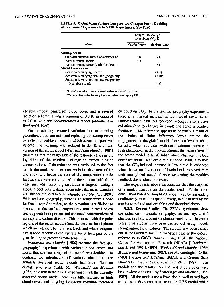
TABLE 5. Global Mean Surface Temperature Changes Due to Doubling Atmospheric CO 2 Amounts in GFDL Experiments (See Text)
Temperature change on doubling CO z, K
Model Original value Revised value*
Swamp ocean One-dimensional r adiative-conv ective
Annual mean, sector Annual mean, sector (variable cloud)
Mixed layer ocean Seasonally varying, sector Seasonally varying, realistic geography Seasonally varying, realistic geography
(variable cloud)
2.4 2.0
2.9 3.0
(2.4)t (2.0)t
4.0
*Includes results using a revised radiative transfer scheme.
'•Value obtained by halving the results for quadrupling CO 2.
variable (model generated) cloud cover and a revised radiation scheme, giving a warming of 3.0 K, as opposed to 2.0 K with the one-dimensional model [Manabe and Wetheraid, 1980].
On introducing seasonal variation but maintaining prescribed cloud amounts, and replacing the swamp ocean by a 68-m mixed-layer ocean in which ocean transport was ignored, the warming was reduced to 2.4 K with this version of the sector model [Wetheraid and Manabe, 1981] (assuming that the magnitude of the response varies as the logarithm of the fractional change in carbon dioxide concentration). This reduction was attributed to the fact that in the model with seasonal variation the extent of ice
and snow and hence the size of the temperature albedo feedback are severely curtailed in the summer half of the year, just when incoming insolation is largest. Using a global model with realistic geography, the mean warming was further reduced to 2 K [Manabe and Stouffer, 1980]. With realistic geography, there is no temperature albedo feedback over Antarctica, as the elevation is sufficient to
ensure that the surface temperatures remain well below freezing with both present and enhanced concentrations of atmospheric carbon dioxide. This contrasts with the polar regions of the sector models (and the northern hemisphere) which are warmer, being at sea level, and Where tempera- ture albedo feedbacks can operate for at least part of the year, leading to greater climate sensitivity.
Wetheraid and Manabe [1986] repeated the "realistic geography" experiment with variable cloud cover and found that the sensitivity of the model was doubled. In contrast, the introduction of variable cloud into the annually averaged sector models had little effect on climate sensitivity (Table 5). Wetheraid and Manabe [ 1988] note that in their 1980 experiment with the annually averaged sector model there was little increase in high cloud cover, and outgoing long-wave radiation increased
on doubling CO 2. In the realistic geography experiment, there is a marked increase in high cloud cover at all latitudes which leads to a reduction in outgoing long-wave radiation (due to changes in cloud) and hence a positive feedback. This difference appears to be partly a result of the choice of finite difference levels around the
tropopause: in the global model, there is a level at about 95 mbar which coincides with the maximum increase in
high cloud cover in the tropics, whereas the nearest level in the sector model is at 70 mbar where changes in cloud cover are small. Wetheraid and Manabe [1988] also note
that the CO2-induced increase in low cloud is enhanced when the seasonal variation of insolation is removed from
their new global model, further weakening the positive feedback due to cloud processes.
The experiments above demonstrate that the response of a model depends on the model used. Furthermore, conclusions based on simplified models may be misleading qualitatively as well as quantitatively, as illustrated by the studies with fixed and variable cloud described above.
5.3.2. Recent Studies The GFDL experiments show the influence of realistic orography, seasonal cycle, and changes in cloud amount on climate sensitivity. In recent years, five studies have been carried out using models incorporating these features. The studies have been carried out at the Goddard Institute for Space Studies (henceforth referred to as GISS) [Hansen et al., 1984], the National Center for Atmospheric Research (NCAR) [Washington and Meehl, 1984], GFDL [Wetheraid and Manabe, 1986; Manabe and Wetheraid, 1987], the Meteorological Office (MO) [Wilson and Mitchell, 1987a], and Oregon State University (OSU) [Schlesinger and Zhao, 1987]. The models and the results from the first three studies have
been reviewed in detail by Schlesinger and Mitchell [ 1985, 1987]. All the models use a fixed-depth, well-mixed layer to represent the ocean, apart from the GISS model which
Mitchell: "GREENHOUSE" EFFECT 27,1 / REVIEWS OF GEOPHYSICS ß 127
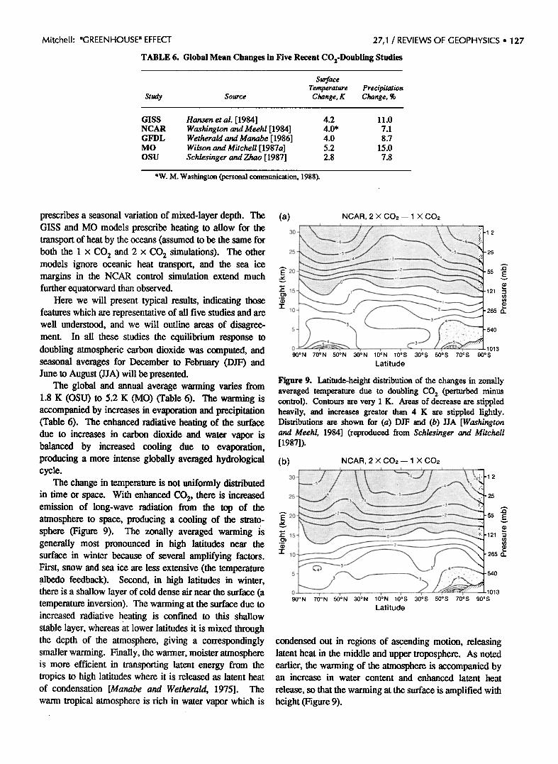
TABLE 6. Global Mean Changes in Five Recent CO2-Doubling Studies
Surface Temperature Precipitation
Study Source Change, K Change, %
GISS Hansen et al. [ 1984] 4.2 11.0 NCAR Washington and Meehl [1984] 4.0* 7.1 GFDL Wetheraid and Manabe [ 1986] 4.0 8.7 MO Wilson and Mitchell [ 1987a] 5.2 15.0 OSU Schlesinger and Zhao [ 1987] 2.8 7.8
*W. M. Washington (personal communication, 1988).
prescribes a seasonal variation of mixed-layer depth. The GISS and MO models prescribe heating to allow for the transport of heat by the oceans (assumed to be the same for
both the 1 x CO 2' and 2 x CO 2 simulations). The other models ignore oceanic heat transport, and the sea ice margins in the NCAR control simulation extend much further equatorward than observed.
Here we will present typical results, indicating those features which are representative of all five studies and are well understood, and we will outline areas of disagree- ment. In all these studies the equilibrium response to doubling atmospheric carbon dioxide was computed, and seasonal averages for December to February (DJF) and June to August (JJA) will be presented.
The global and annual average warming varies from 1.8 K (OSU) to 5.2 K (MO) (Table 6). The warming is accompanied by increases in evaporation and precipitation (Table 6). The enhanced radiative heating of the surface due to increases in carbon dioxide and water vapor is balanced by increased cooling due to evaporation, producing a more intense globally averaged hydrological cycle.
The change in temperature is not uniformly distributed in time or space. With enhanced CO 2, there is increased emission of long-wave radiation from the top of the atmosphere to space, producing a cooling of the strato- sphere (Figure 9). The zonally averaged warming is generally most pronounced in high latitudes near the surface in winter because of several amplifying factors. First, snow and sea ice are less extensive (the temperature albedo feedback). Second, in high latitudes in winter, there is a shallow layer of cold dense air near the surface (a temperature inversion). The warming at the surface due to increased radiative heating is confined to this shallow stable layer, whereas at lower latitudes it is mixed through the depth of the atmosphere, giving a correspondingly smaller warming. Finally, the warmer, moister atmosphere is more efficient in transporting latent energy from the tropics to high latitudes where it is released as latent heat of condensation [Manabe and Wetheraid, 1975]. The warm tropical atmosphere is rich in water vapor which is
(a) NCAR, 2 X CO2- 1 X CO2
0 55
0•15 121 © ,
10 • z 265 r'• 5 ' :' •.' ";'.-:- ' : ' : 540
0 1013 90øN 70øN 50øN 30øN 10øN 10øS 30øS 50øS 70øS 90øS
Latitude
Figure 9. Latitude-height distribution of the changes in zonally averaged temperature due to doubling CO 2 (perturbed minus control). Contours are very 1 K. Areas of decrease are stippled heavily, and increases greater than 4 K are stippled lightly. Distributions are shown for (a) DJF and (b) JJA [Washington and Meehl, 1984] (reproduced from Schlesinger and Mitchell [19871).
(b) NCAR, 2 X CO2- 1 X CO2
10 265 •_.
3 3 4
5 3 • • ." .":;:";'-".'. . 540 •3 ;"" ' :":. '.
90øN 71•øN 50•ON 30•ON 10ON 10øS 30øS 50øS 70øS 90øS Latitude
condensed out in regions of ascending motion, releasing latent heat in the middle and upper troposphere. As noted earlier, the warming of the atmosphere is accompanied by an increase in water content and enhanced latent heat
release, so that the warming at the surface is amplified with height (Figure 9).

128 ß REVIEWS OF GEOPHYSICS / 27,1 Mitchell: "GREENHOUSE" EFFECT
SURFACE AIR TEMPERATURE DIFFERENCES
GISS, 2 X CO2- 1 X CO2 DdF
90ON I I _ . I I I I . I
.............. ....... '•' "'.•'•-I0 '... ß ß '.': :...•:..::•:".:iit :?' ,:!:'..::: ..... "":':"::::'" :":":'•:'""•' ....... i Io !%' '
30 ø
"6 ' ' .... 4 , .' ..... :: '.".."".:"
9oos - I ..... I i i I i i i ! 0 ø 60 ø 120 ø E 180 ø 120 ø W 60 ø 0 ø
Figure 10. Changes in surface temperature due to doubling CO 2 for (a) DJF and (b) JJA. Contours are ever), 2 K, and increases greater than 4 K are stippled [Hansen et al., 1984] (reproduced from Schlesinger and Mitchell [1987]).
GISS, 2 X CO2- 1 X CO2 JJA I I I I I I I
(b) 90ø N- ::•
60ø- ••4 4•• •"' '•'•••4 '•.:: • •::: 4. ". .
0 o
30ø -• 4
I I I 0 ø 60 ø 120 ø E 180 ø 120 ø W 60 ø 0 ø
The simulated changes in temperature also vary considerably with longitude and season (Figure 10). The largest warming occurs over sea ice in winter; the smallest over sea ice in summer. In summer, sea ice in the Arctic is
maintained at freezing level by the melting of ice. With enhanced CO 2 , either more sea ice is melted, producing no change in surface temperature, or the sea ice melts completely, leaving the underlying oceanic mixed layer which limits the rise in temperature through its large thermal inertia. On the other hand, the reduction in surface
albedo due to removing sea ice leads to increased absorp- tion of solar radiation. This extra energy is stored in the mixed layer and released in autumn and winter, delaying
the onset of freezing and leading to thinner sea ice. More heat can diffuse through the thinner sea ice, also contribut- ing to the enhanced surface warming in winter [Manabe and Stouffer, 1980].
There is also a considerable geographical variation in warming within individual continents. In regions where the soil becomes drier, evaporation may be restricted, leading to increased warming and vice versa [Manabe et al., 1981]. Local changes in cloud amount may also contribute to the regional variations, especially where insolation is significant. Although the large-scale features of the simulated temperature changes are consistent from model to model, the details vary considerably.

Mitchell: "GREENHOUSE" EFFECT 27,1 / REVIEWS OF GEOPHYSICS ß 129
(a) 180 ø 120 ø W 60 ø 0 ø 60 ø 120 ø E 1 •
90øN ! • i I [ • I I I I • •
...... 30 ø o -. .... 0 :::::::::::::::::::::::::: ......... .ii'"'•:. • -..::!:i" • ...::i:i:i:i:iiii!iiiiiiiiiiiiiiii!iiii ::'"'"'::!'i!i': ::::::::::::::::::::::
o
30 ø
60 ø
90 ø S i • i • i i •oo •oow •oo ' oo •oo ' ' 120 ø E
30 ø
90øN
60 ø
30 ø
-0 o
30 ø
- 60 ø
90øS
180 ø
Figure 11. Changes in precipitation due to doubling CO 2 for (a) DJF and (b) JJA. Contours are at 0, + 1, and + 2 mm d-l, and areas of decrease are stippled [from Wilson and Mitchell, 1987a].
(b) 180 ø 120øW 60 ø 0 o 60 ø 120øE 180 ø
90 ø N i ===================================:'•1 I L '___l ' ' ' F-I ' _ 90 ø N o.1' (A-l "0 ' o
1 1 ..:!iiiii!iiii!:ii!iii!::i:!:::::'::.i:::::i::::'i:i:i:::::-'.' 0 •-..• (• ..... '." .½:.:!:...::: ['!:!:i:::.-. 1 ½, C..• • 30 ø- ::)•- 30':'
0 o ======================================================= .... •.___...__./_ 0 o
30 ø - ............. '"•- 30':' 600 -L '""• - ,.._,_ • •____.•_•_• 1• • 60ø
90 ø S I , • ' • ' • ' • , • i 90 S 180 ø 120 ø W 60 ø 0 ø 60 ø 120 ø E 180 ø
With the increase in atmospheric moisture accompany- ing the warming due to enhanced CO 2 one would expect precipitation to increase in the main regions of low-level atmospheric convergence, including the extratropical depression belts and the Intertropical Convergence Zone [Mitchell et al., 1987]. There is a general increase in precipitation in high latitudes, especially in winter (Figure 11), consistent with increased moisture transport from low latitudes. The changes in the Intertropical Convergence Zone (ITCZ) vary considerably from model to model, with, for example, the GFDL and MO models producing marked increases in monsoon precipitation over southeast Asia and the NCAR and GISS models producing decreases. In the subtropics, precipitation changes little or decreases slightly. Apart from high latitudes, there is, as yet, little agreement in the regional changes in precipita-
tion simulated by the different models. Precipitation depends on many small-scale phenomena: orography, land-sea contrasts, and transient atmospheric disturbances, all of which are degraded in low-resolution models. However, many of the features found in the MO experi- ment, including the enhancement of the summer mon- soons, have also been obtained using higher-resolution models with prescribed increases in sea surface tempera- tures [Mitchell and Lupton, 1984; Mitchell et al., 1986, 1987].
In determining the availability of moisture at the surface, changes in evaporation as well as precipitation have to be taken into account. In current models, precipitation and snowmelt are accumulated at each grid point in what can be regarded as a "bucket," typically 15 cm deep. Any "overflow," corresponding to saturation of
130 ß REVIEWS OF GEOPHYSICS / 27,1 Mitchell: "GREENHOUSE" EFFECT
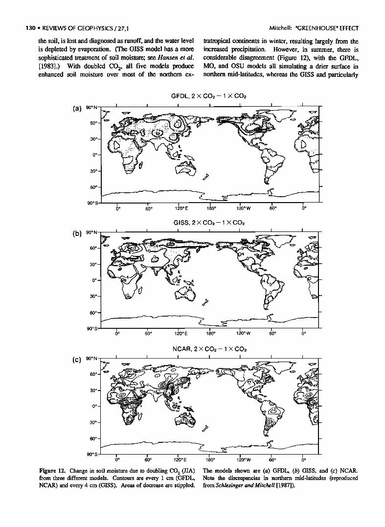
the soil, is lost and diagnosed as ranoff, and the water level is depleted by evaporation. (The GISS model has a more sophisticated treatment of soil moisture; see Hansen et al. [1983].) With doubled CO 2, all five models produce enhanced soil moisture over most of the northern ex-
tintropical continents in winter, resulting largely from the increased precipitation. However, in summer, there is considerable disagreement (Figure 12), with the GFDL, MO, and OSU models all simulating a drier surface in northern mid-latitudes, whereas the GISS and particularly
GFDL, 2 X CO2- 1 X CO2
60 ø --
60 o --
90øS I I I 0 o 60 ø 120OE
I I I I 180 ø 120 ø W 60 ø 0 ø
(b) 90øN
G ISS, 2 X CO2- 1 X CO2
t30 ø - --
30 ø
•øø •• 90øS • • '" I • i I 0 ø 60 ø 120 ø [ 180 ø 1 •0 ø W 60 ø 0 ø
90 ø N-
(c) 60 ø -
30 ø -
0 o -
30 ø -
60 o -
90os -
NCAR, 2 X CO2- 1 X CO2 I I I I I I I ,_
I i i
0 o 60 ø 120 ø E I I ! I
180 ø 120 ø W 60 ø 0 ø
Figure 12. Change in soil moisture due to doubling CO 2 (JJA) from three different models. Contours are every 1 cm (GFDL, NCAR) and every 4 cm (GISS). Areas of decrease are stippled.
The models shown are (a) GFDL, (b) GISS, and (c) NCAR. Note the discrepancies in northern mid-latitudes (reproduced from Schlesinger and Mitchell [1987]).
Mitchell: "GREENHOUSE" EFFECT
the NCAR models exhibit a widespread increase in soil moisture. As this area contains the world's major grain- growing regions, which already are vulnerable to drought, there is considerable interest as to which of the simulations
are correct.
In those studies producing a summer drying in northern latitudes the following factors have been found to con- tribute: increased evaporation due to enhanced radiative heating from the warmer, moister, CO2-enriched atmos- phere; earlier snowmelt, especially in high latitudes; and reduced cloud and precipitation, at least in more southerly latitudes [Manabe et al., 1981; Manabe and Wetheraid,
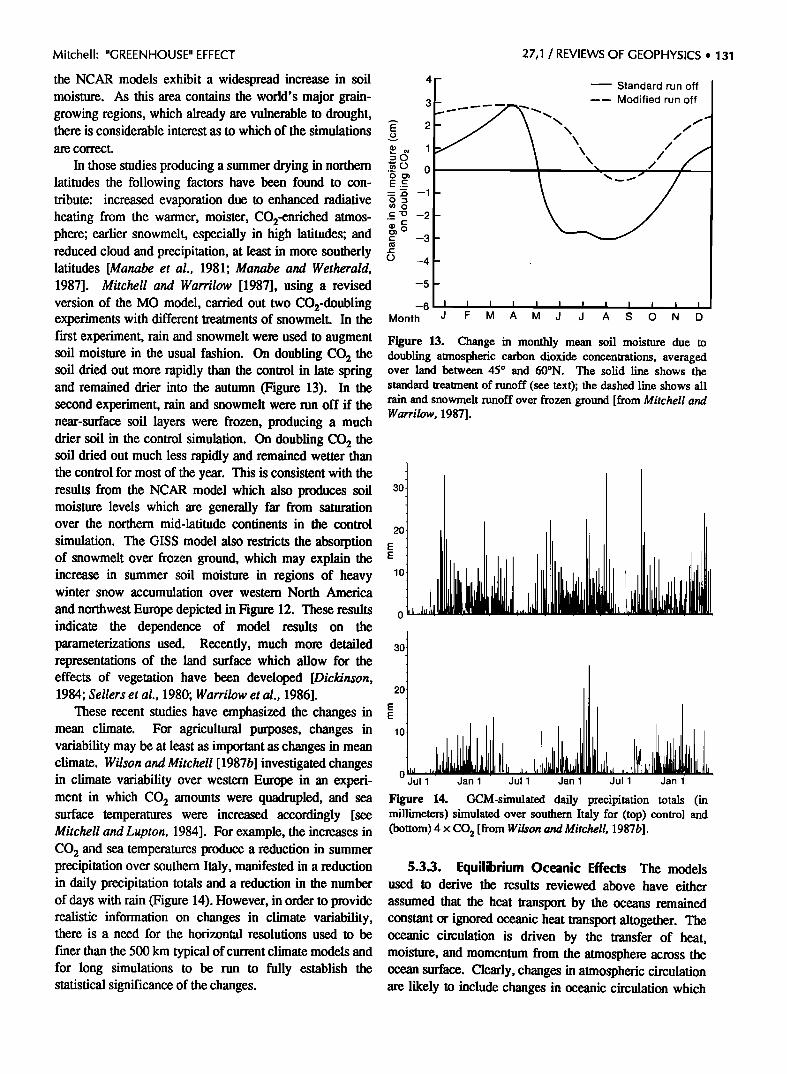
1987]. Mitchell and Warrilow [1987], using a revised version of the MO model, carried out two CO2-doubling experiments with different treatments of snow•nelt. In the first experiment, rain and snowmelt were used to augment soil moisture in the usual fashion. On doubling CO• the soil dried out more rapidly than the control in late spring and remained drier into the autumn (Figure 13). In the second experiment, rain and snowmelt were run off if the near-surface soil layers were frozen, producing a much drier soil in the control simulation. On doubling CO• the soil dried out much less rapidly and remained wetter than the control for most of the year. This is consistent with the results from the NCAR model which also produces soil moisture levels which are generally far from saturation over the northern mid-latitude continents in the control
simulation. The GISS model also restricts the absorption of snowmelt over frozen ground, which may explain the increase in summer soil moisture in regions of heavy winter snow accumulation over western North America
and northwest Europe depicted in Figure 12. These results indicate the dependence of model results on the parameterizations used. Recently, much more detailed representations of the land surface which allow for the effects of vegetation have been developed [Dickinson, 1984; Sellers et al., 1980; Warrilow et al., 1986].
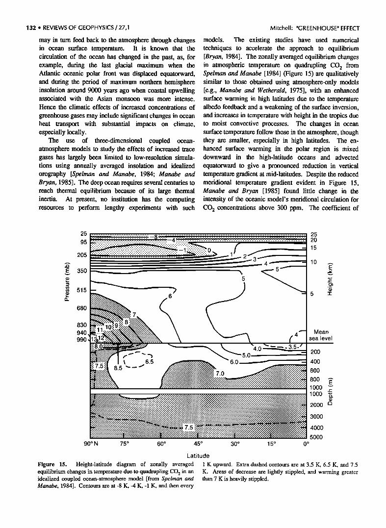
These recent studies have emphasized the changes in mean climate. For agricultural purposes, changes in variability may be at least as important as changes in mean climate. Wilson and Mitchell [1987b] investigated changes in climate variability over western Europe in an experi- ment in which CO• amounts were quadrupled, and sea surface temperatures were increased accordingly [see Mitchell and Lupton, 1984]. For example, the increases in CO• and sea temperatures produce a reduction in summer precipitation over southern Italy, manifested in a reduction in daily precipitation totals and a reduction in the number of days with rain (Figure 14). However, in order to provide realistic information on changes in climate variability, there is a need for the horizontal resolutions used to be
finer than the 500 km typical of current climate models and for long simulations to be run to fully establish the statistical significance of the changes.
27,1 / REVIEWS OF GEOPHYSICS ß 131
4 F Standard run off 3 !- • ---- Modified run off
=O
•o 0 - '• o•
ß • •= - o• O
•o
-4
-6 i • I I I I I I I I I I Month J F M A M J J A S O N D
Figure 13. Change in monthly mean soil moisture due to doubling atmospheric carbon dioxide concentrations, averaged over land between 45 ø and 60øN. The solid line shows the
standard treatment of runoff (see text); the dashed line shows all rain and snowmelt ranoff over frozen ground [from Mitchell and Warrilow, 1987].
30
20
30
Jul 1 Jan 1 Jul 1
I
Jan 1 Jul 1 Jan 1
Figure 14. GCM-simulated daily precipitation totals (in millimeters) simulated over southern Italy for (top) control and (bottom) 4 x CO 2 [from Wilson and Mitchell, 1987b].
5.3.3. Equilibrium Oceanic Effects The models used to derive the results reviewed above have either assumed that the heat transport by the oceans remained constant or ignored oceanic heat transport altogether. The oceanic circulation is driven by the transfer of heat, moisture, and momentum from the atmosphere across the ocean surface. Clearly, changes in atmospheric circulation are likely to include changes in oceanic circulation which
13:2 ß REVIEWS OF GEOPHYSICS / 27,1
may in turn feed back to the atmosphere through changes in ocean surface temperature. It is known that the circulation of the ocean has changed in the past, as, for example, during the last glacial maximum when the Atlantic oceanic polar front was displaced equatorward, and during the period of maximum northern hemisphere insolation around 9000 years ago when coastal upwelling associated with the Asian monsoon was more intense.
Hence the climatic effects of increased concentrations of
greenhouse gases may include significant changes in ocean heat transport with substantial impacts on climate, especially locally.
The use of three-dimensional coupled ocean- atmosphere models to study the effects of increased trace gases has largely been limited to low-resolution simula- tions using annually averaged insolation and idealized orography [Spelman and Manabe, 1984; Manabe and Bryan, 1985]. The deep ocean requires several centuries to reach thermal equilibrium because of its large thermal inertia. At present, no institution has the computing resources to perform lengthy experiments with such
Mitchell: "GREENHOUSE" EFFECT
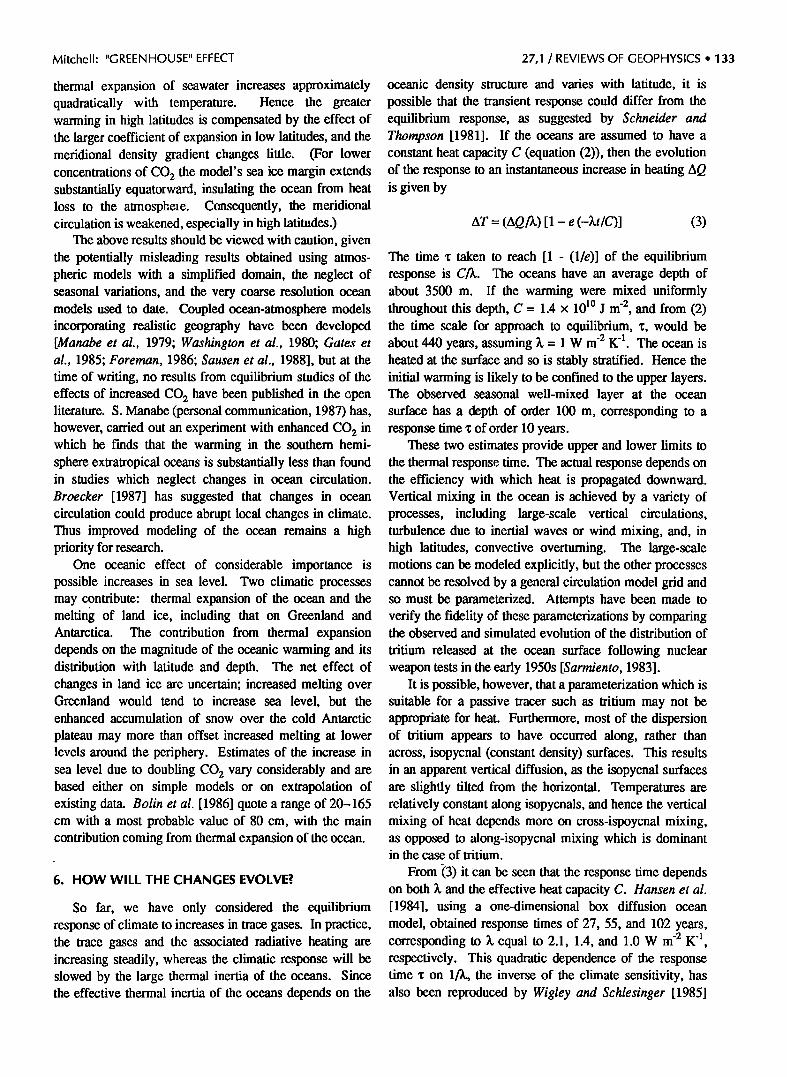
models. The existing studies have used numerical techniques to accelerate the approach to equilibrium [Bryan, 1984]. The zonally averaged equilibrium changes in atmospheric temperature on quadrupling CO 2 from Spelman and Manabe [1984] (Figure 15) are qualitatively similar to those obtained using atmosphere-only models [e.g., Manabe and Wetheraid, 1975], with an enhanced surface warming in high latitudes due to the temperature albedo feedback and a weakening of the surface inversion, and increases in temperature with height in the tropics due to moist convective processes. The changes in ocean surface temperature follow those in the atmosphere, though they are smaller, especially in high latitudes. The en- hanced surface warming in the polar region is mixed downward in the high-latitude oceans and advected equatorward to give a pronounced reduction in vertical temperature gradient at mid-latitudes. Despite the reduced meridional temperature gradient evident in Figure 15, Manabe and Bryan [1985] found little change in the intensity of the oceanic model's meridional circulation for CO2 concentrations above 300 ppm. The coefficient of
25
95
205
350
515
680
83O
94O
990
......... ' ,œ ,*
...:::::•.••••.. . ...... ..... , 2•3•-- 4•'-• - 10
,..., :• :...: :....::..••• :• :'''"'' ':'••'"' • :....•• 6 5 T '-•." "::::::-."::::'. ::::::::::::::::::::::::::::::: 4 Mean
ß , , _ , ::::.-'•---,'.].',•.•ii- :•'•;'•"'""' 4.0 •- :3.5- 200
i!i_7.5 !ii 8.5 - - ½ ' 400 •.'.'.'.-.'. ..:.:.:.:-:-:-:-:-:-:.:.:.:.:-:-:-:.:-:.:.:-:-: . ..:.:-:.:............................. 600
2000 :.•:•.:.•F:•:.:•:•:M:•:•:•:•:•:•:•:•:M:M:•:•:•:M:M:i:•:•:•:•:•:M:•:•:•:•:•:•:•:•:•:•:•:•:•:M:•:•:M:•:M:•:•:M:•:•:•:•:•:•:M:•:•:i:i:•:•:•:•:i:•:•:M:i:M:•E•:• 3000 .......-...-.-.. .... •.•.•n.•..-•.....•.•.•.•.•.•.•.:.:.:.:•:.:•:.:.:.:•:•:.:•:•:.:•:•:•:.:.:•:.:.:.:.:.:.:.:•:.:•:•:.:•:.:.:•:.:•:.:•:.:•:•:•:.:.:.:.:.:•:•:•:•:.:•:•:.:•:•:.:•:•:.:•:•:.:.•.•:.. ß :.:.:.:.:.:.:.:.:.:.:.:.:.:.:.:.:.2:.:.:.:.:.:'.'.'..' .• '."::::::::::. :. :. :. :. :. :. :. :. '. '. '. '. '. '. :. :. :. :. :. :. :. :4. :. :. :. :. :' :-:' :' :' :' ::',•-:" ',a,•::•;i:' ',444. ',444. ',4•. '•b4. :444. :.-•. • :.:.:.:.:.:.:•:•:•:•:.:•:.:•:•:.:.:.:•:.:•:.:•:.:.:•:•:•:•:.:.•...':.•..•.n4.•..•..•.• '• •' "'.n'•. "nnn"'-'-nn" 'nnnn"w'"w" ......... '"'""'"'"'"""":'"":':':':':':':':':':':': .?..:.:.:.:.:.:.:.:.:.:.:.:.:.:.:.:.:.:.:.:.:.:.:.:.:.:.:.:.:.:.:.::::::.:.........•....::?.. /. O :::::::::::::::::::::::::::::::::::::::::::::::::::::::::::::::::::::::::::::::::::::::::::::::::::::::::::::: 4000
.ooo 90 ø N 75 ø 60 ø 45 ø 30 ø 15 ø 0 ø
Latitude
Figure 15. Height-latitude diagram of zonally averaged 1 K upward. Extra dashed contours are at 3.5 K, 6.5 K, and 7.5 equilibrium changes in temperature due to quadrupling CO 2 in an K. Areas of decrease are lightly stippled, and warming greater idealized coupled ocean-atmosphere model [f•om Spelman and than 7 K is heavily stippled. Manabe, 1984]. Contours are at-8 K,-4 K, -1 K, and then every
Mitchell: "GREENHOUSE" EFFECT 27,1 / REVIEWS OF GEOPHYSICS ß 133
thermal expansion of seawater increases approximately quadratically with temperature. Hence the greater warming in high latitudes is compensated by the effect of the larger coefficient of expansion in low latitudes, and the meridional density gradient changes little. (For lower concentrations of CO 2 the model's sea ice margin extends substantially equatorward, insulating the ocean from heat loss to the atmosphere. Consequently, the meridional circulation is weakened, especially in high latitudes.)
The above results should be viewed with caution, given the potentially misleading results obtained using atmos- pheric models with a simplified domain, the neglect of seasonal variations, and the very coarse resolution ocean models used to date. Coupled ocean-atmosphere models incorporating realistic geography have been developed [Manabe et al., 1979; Washington et al., 1980; Gates et al., 1985; Foreman, 1986; Sausen et al., 1988], but at the
time of writing, no results from equilibrium studies of the effects of increased CO 2 have been published in the open literature. S. Manabe (personal communication, 1987) has, however, carried out an experiment with enhanced CO2 in which he finds that the warming in the southern hemi- sphere extratropical oceans is substantially less than found in studies which neglect changes in ocean circulation. Broecker [1987] has suggested that changes in ocean circulation could produce abrupt local changes in climate. Thus improved modeling of the ocean remains a high priority for research.
One oceanic effect of considerable importance is possible increases in sea level. Two climatic processes may contribute: thermal expansion of the ocean and the meltin g of land ice, including that on Greenland and Antarctica. The contribution from thermal expansion depends on the magnitude of the oceanic warming and its distribution with latitude and depth. The net effect of changes in land ice are uncertain; increased melting over Greenland would tend to increase sea level, but the enhanced accumulation of snow over the cold Antarctic
plateau may more than offset increased melting at lower levels around the periphery. Estimates of the increase in sea level due to doubling CO2 vary considerably and are based either on simple models or on extrapolation of existing data. Bolin et al. [1986] quote a range of 20-165 cm with a most probable value of 80 cm, with the main contribution coming from thermal expansion of the ocean.
6. HOW WILL THE CHANGES EVOLVE z.
So far, we have only considered the equilibrium response of climate to increases in trace gases. In practice, the trace gases and the associated radiative heating are increasing steadily, whereas the climatic response will be slowed by the large thermal inertia of the oceans. Since the effective thermal inertia of the oceans depends on the
oceanic density structure and varies with latitude, it is possible that the transient response could differ from the equilibrium response, as suggested by Schneider and Thompson [1981]. If the oceans are assumed to have a constant heat capacity C (equation (2)), then the evolution of the response to an instantaneous increase in heating AQ is given by
AT = (AQ/X) [1 - e (-)•t/C)] (3)
The time x taken to reach [1 - (l/e)] of the equilibrium response is C/Z. The oceans have an average depth of about 3500 m. If the warming were mixed uniformly throughout this depth, C = 1.4 x 10 •ø J m '2, and from (2) the time scale for approach to equilibrium, x, would be about 440 years, assuming )• = 1 W m '2 K '•. The ocean is heated at the surface and so is stably stratified. Hence the initial warming is likely to be confined to the upper layers. The observed seasonal well-mixed layer at the ocean surface has a depth of order 100 m, corresponding to a response time x of order 10 years.
These two estimates provide upper and lower limits to the thermal response time. The actual response depends on the efficiency with which heat is propagated downward. Vertical mixing in the ocean is achieved by a variety of processes, including large-scale vertical circulations, turbulence due to inertial waves or wind mixing, and, in high latitudes, convective overturning. The large-scale motions can be modeled explicitly, but the other processes cannot be resolved by a general circulation model grid and so must be parameterized. Attempts have been made to verify the fidelity of these parameterizations by comparing the observed and simulated evolution of the distribution of
tritium released at the ocean surface following nuclear weapon tests in the early 1950s [Sarmiento, 1983].
It is possible, however, that a parameterization which is suitable for a passive tracer such as tritium may not be appropriate for heat. Furthermore, most of the dispersion of tritium appears to have occurred along, rather than across, isopycnal (constant density) surfaces. This results in an apparent vertical diffusion, as the isopycnal surfaces are slightly tilted from the horizontal. Temperatures are relatively constant along isopycnals, and hence the vertical mixing of heat depends more on cross-ispoycnal mixing, as opposed to along-isopycnal mixing which is dominant in the case of tritium.
From (3) it can be seen that the response time depends on both )• and the effective heat capacity C. Hansen et al. [1984], using a one-dimensional box diffusion ocean model, obtained response times of 27, 55, and 102 years, corresponding to 3. equal to 2.1, 1.4, and 1.0 W m '2 K '•, respectively. This quadratic dependence of the response time x on 1/)•, the inverse of the climate sensitivity, has also been reproduced by Wigley and Schlesinger [1985]
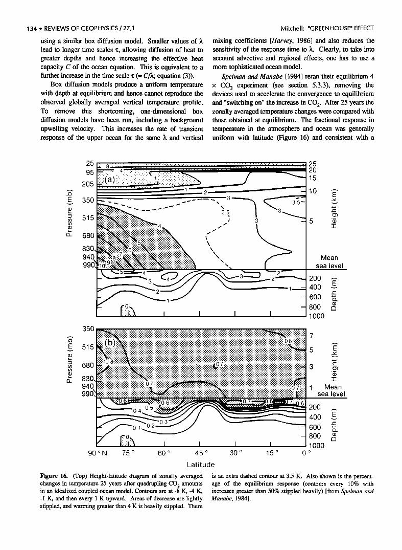
134 ß REVIEWS OF GEOPHYSICS / 27,1 Mitchell: "GREENHOUSE" EFFECT
using a similar box diffusion model. Smaller values of A, lead to longer time scales x, allowing diffusion of heat to greater depths and hence increasing the effective heat capacity C of the ocean equation. This is equivalent to a further increase in the time scale x (= C/•; equation (3)).
Box diffusion models produce a uniform temperature with depth at equilibrium and hence cannot reproduce the observed globally averaged vertical temperature profile. To remove this shortcoming, one-dimensional box diffusion models have been run, including a background upwelling velocity. This increases the rate of transient response of the upper ocean for the same A, and vertical
mixing coefficients [Harvey, 1986] and also reduces the sensitivity of the response time to 3.. Clearly, to take into account advective and regional effects, one has to use a more sophisticated ocean model.
Spelman and Manabe [1984] reran their equilibrium 4 x CO 2 experiment (see section 5.3.3), removing the devices used to accelerate the convergence to equilibrium and "switching on" the increase in CO 2. After 25 years the zonally averaged temperature changes were compared with those obtained at equilibrium. The fractional response in temperature in the atmosphere and ocean was generally uniform with latitude (Figure 16) and consistent with a
E 350 •'- ,
205 '- "'-'••'-'"'-'.'.•.: .......'•.'.'.'.0 -'}.-----'--•• • 2 • •
3•
515
68O
83O ½
990
1- i
I I I
25 2O
15
10
5
Mean
sea level
2OO
4OO
6OO
8OO
1000
35O
515
940 !!iiii!!iiiiiii!iii!.O 7:.:.:.:.:.:.:.:. ::::::::::::::::::::::::::::::::::: ............................... 1 .................... .o......o.o......O..oO...o........oOo.,.....o..O..o ......
99 ======================== ' ...................... Mean
sea level
04
01
90 øN 75 o 60 o 45 o 30 o 15 o
Latitude
200
400
600
8OO
1000 0 ø
Figure 16. (Top) Height-latitude diagram of zonally averaged changes in temperature 25 years after quadrupling CO 2 amounts in an idealized coupled ocean model. Contours are at -8 K, -4 K, -1 K, and then every 1 K upward. Areas of decrease are lightly stippled, and warming greater than 4 K is heavily stippled. There
is an extra dashed contour at 3.5 K. Also shown is the percent- age of the equilibrium response (contours every 10% with increases greater than 50% stippled heavily) [from Spelman and Manabe, 1984].

Mitchell' "GREENHOUSE" EFFECT 27,1 / REVIEWS OF GEOPHYSICS ß 135
response time 'c of about 25 years using (3). The greatest penetration of the warming into the ocean occurs near 55 ø . In higher latitudes an excess of precipitation over evapora- tion produced a stable layer of fresh, less dense water at the surface and confined the warming to the surface. The oceanic response is discussed in more detail by Bryan and Spelman [1985]. Schlesinger [1986] estimated that the thermal response time of the ocean was 75-100 years on the basis of a 16-year "switch on" experiment with doubled CO 2 carried out using a coupled ocean-atmosphere model which included the diurnal cycle and realistic geography. Harvey [1986] reanalyzed Schlesinger's [1986] results and arrived at a time scale nearer to 50 years. An accurate estimate of the thermal response time is essential for the detection of man-induced climate change, which is discussed later.
Spelman and Manabe [1984] point out that if the characteristic time scale of the oceanic response is less than that of the increase in trace gases, then the distribution of the zonally averaged temperature response to a gradual increase in trace gases may resemble the distribution of the equilibrium response. Hence both the rate at which climate responds to increases in trace gases and the geographical distribution of the time-dependent response may depend critically on the magnitude of the feedback strength 3,.
7. WHEN WILL WE BE ABLE TO DETECT THE
CLIMATIC EFFECTS?
Given that the estimated increase in trace gases since 1860 is equivalent to a 40% increase in CO 2, it is pertinent to ask if the climatic effects can be detected in the
observational record. The answer to this question is obscured by the accumulated effects of several uncertainties.
1. There are uncertainties in the preindustrial levels of trace gases, particularly carbon dioxide, methane, and tropospheric ozone (section 4). For example, the range of the estimates of preindustrial CO 2 concentration, 260-290 ppm, introduces an error of + 0.3 W m '2 in the current greenhouse effect (Table 3).
2. There are uncertainties in the sensitivity of climate. Estimates of the equilibrium sensitivity of climate differ by a factor of 3 [Bolin et al., 1986]. Much of this uncertainty is due to the uncertainty in cloud feedbacks. Current model simulations indicate a feedback strength 3, of about 1 W m '2 K '• which could be increased•to 2.0 W m '2 K '• if the net cloud feedback is neutral (see Table 4). Assuming AQ = 1.9 W m '2 (Table 3) and a feedback strength of between 1.0 and 2.0 W m '2 K '•, we can estimate that the equilibrium warming due to increases in trace gases to date lies between 1.0 and 1.9 K.
3. There is a lack of knowledge concerning the effective thermal inertia of the oceans. There is consider-
able uncertainty in the degree to which the thermal inertia of the ocean will slow the warming. This is compounded by the uncertainty in the estimates of 3,. As discussed in section 6, the response time of the idealized system described in section 5 is C/X = CAT•/AQ where AT• is the equilibrium temperature change. As a result, the larger the equilibrium response, the smaller the fractional response in a given time (equation (3)), so that the magnitude of the response on a short time scale is only weakly dependent on the magnitude of the equilibrium response. As a conse- quence, a small range in the magnitude of the current observed response is compatible with a large range of equilibrium responses. Thus the observed temperature changes will only provide a weak constraint on the magnitude of climate sensitivity. (This in turn means that one can only make a rough estimate of the final equilib- rium warming which would occur with no further increases in trace gases.)
The magnitude of the expected warming to date has been estimated using one-dimensional models [Hansen et al., 1981; Wigley and Schlesinger, 1985]. If one ignores the increase in chlorofluorocarbons, which has been
confined to the last two decades, the increase in heating since 1880 is about 1.7 W m '2, equivalent to the effect of increasing CO 2 from 250 ppm to its current value. On the basis of Wigley and Schlesinger's assumptions the warming to date ranges from just under 0.5 K (large vertical mixing coefficient, )• = 2.0 W m '2 K '•) to over 1 K (small vertical mixing coefficient, 3, = 1.0 W m '2 K4).
0.5
øC 0.0
1900 1920 1940 1960 19 0 2000 Year
Figure 17. Observed global surface air temperature anomalies, 1901-1987 [Jones et al., 1988]. Copyright 1988 Macmillan Magazines Ltd; reprinted with permission.
4. There is considerable variability in the observed temperature record. Global mean surface temperature has increased by about 0.4 K since 1900 (see Figure 17 [from Jones et al., 1988]). The warmest year on record was 1987. The increase has been far from uniform, with
marked year to year variability and a period of cooling

136 ß REVIEWS OF GEOPHYSICS / 27,1
after 1940. Clearly, this cooling is not due to increases in trace gases. It may be a manifestation of the natural variability of the ocean-atmosphere system, or it may be due to external causes such as a decrease in solar
luminosity or an increase in volcanic aerosols. Prior to this period, land data analyzed by P. D. Jones et al. [1986] suggest that global mean temperatures were relatively constant from 1860 to 1900, whereas marine air data
[Parker et al., 1988] suggest that temperatures were two or three tenths of a degree warmer in 1860 than in 1900.
The observed warming from 1900 is slightly smaller than the lower estimates given above. However, the waxming due to trace gases may be masked by natural variations and the effects of external factors. Thus one
cannot conclude that theoretical estimates of the warming are too high, nor can one conclude that the climatic effects of trace gases have been detected.
Estimates of the warming due to increased greenhouse gas concentrations over the next 50 years are obviously dependent on the projected concentrations of these gases. First, a continued warming is expected as climate comes to equilibrium with the current concentrations of trace gases. Second, the estimates of further increases in trace gas concentrations over the next 50 years (Table 3) imply an additional warming, which on reaching equilibrium would range from 1.8 to 3.5 K. A precise estimate of the actual change in surface temperature over the next 50 years is precluded by uncertainties in the sensitivity of climate and the effect of the thermal inertia of the ocean, but an
additional warming of 1 K or more seems likely. If this is the case, then an unambiguous detection of the warming due to trace gases should be possible within the next two decades. Even if the trace gas amounts remain constant thereafter, the warming will continue until the ocean and atmosphere reach thermal equilibrium.
8. SUMMARY AND CONCLUDING REMARKS
The surface of our planet remains habitable because of the presence of water vapor, carbon dioxide, and ozone in the atmosphere. These gases absorb and emit thermal radiation, raising the global mean surface temperature from 225 K (-18øC) to 288 K (15øC). The absorption occurs because of excitation of vibrational and rotational molecu-
lar states. Because tropospheric temperatures generally decrease with height, the addition of greenhouse gases to the atmosphere raises the mean level from which thermal radiation escapes to space, hence reducing the temperature of emission and the rate of emission. Tropospheric and surface temperatures increase until the outgoing thermal radiation again balances the incoming solar radiation. This is known as the greenhouse effect.
Mitchell: "GREENHOUSE" EFFECT
The atmospheric concentrations of many greenhouse gases, including carbon dioxide, tropospheric ozone, methane, and nitrous oxide, have been observed to increase
over the last few decades. These increases are generally believed to be due to increased industrial and agricultural activity, though all these gases have natural chemical cycles, and with the exception of carbon dioxide our understanding of the detailed causes of the increases is lacking. In the past two decades, other gases, notably chlorofluorocarbons, have been added to the atmosphere. Although they are present in very small quantifies, they are several orders of magnitude more effective per molecule than carbon dioxide in trapping thermal radiation, as they absorb strongly at wavelengths where there is little absorption by the other gases (the atmospheric "window").
The direct radiative effects of increasing major greenhouse gases are well known. It has been estimated that the additional heating due to increases in trace gases since the Industrial Revolution is about 2 W m -2, and in the next 50 years this could easily increase by a further 4 W m -2, though this figure is heavily based on extrapolation of existing trends. The climatic response may be amplified or reduced by changes in water vapor, snow and ice, cloud, and so on. Estimates of the sensitivity of surface tempera- ture to enhanced radiative heating vary from less than 0.5 K W 4 m 2 to over 1 K W -• m 2. Most of this uncertainty arises from difficulties in representing cloud effects faithfully in numerical models. Estimates of the equilib- rium warming due to changes since 1860 range from 1 to 2 K, but the actual warming is estimated at about half these values because of the thermal inertia of the oceans. This is
not inconsistent with the observational record, but one cannot prove that a greenhouse waxming has been detected because of the temporal variability of climate. Estimates of the change over the next 50 years are dependent on the projected increases in trace gases and the assumptions made concerning climate sensitivity and thermal inertia, but a warming of 1 K or more seems likely.
The possible climatic effects have been studied using general circulation models of the atmosphere coupled to simplified models of the ocean and sea ice. The following physical responses (where reported) are common to all recent experiments.
1. There is a warming of the troposphere and surface. In the tropics the warming increases with height and varies little with season. The largest warming occurs over sea ice and surrounding regions in winter, because of the removal or thinning of sea ice and the inherent low-level stability in high latitudes. The warming is generally a minimum over sea ice in summer.
2. Snowmelt occurs earlier, and sea ice is less extensive.
3. The increase in atmospheric temperature is accom- panied by an increase in atmospheric water vapor content,

Mitchell: "GREENHOUSE" EFFECT 27,1 / REVIEWS OF GEOPHYSICS ß 137
further enhancing the radiative heating at the surface. Global mean rates of precipitation and evaporation increase.
4. The geographical distribution of precipitation changes is far from uniform. There is a general increase in precipitation and runoff in high latitudes. Precipitation increases in low latitudes, though locally there are regions of increase and decrease which vary from model to model. In most studies to date, there is a reduction in soil moisture over the northern mid-latitude continents in summer.
5. The magnitude of the response is greatly enhanced in most simulations with model-generated cloud. A decrease in total cloud and an increase in mean cloud
height both contribute to this enhancement. There are several priorities for future research. First,
we need to reduce the uncertainty in the magnitude of climate sensitivity. Here the major shortcoming is our poor understanding of the processes governing the formation and radiative properties of clouds, compounded by the fact that clouds are not resolved by the model grid. The radiative properties of water clouds depend on the cloud water content, which has been parameterized in general circulation models, and the effective droplet radius, which has not. Even less is known about the properties of ice clouds, an area where there is a requirement for further experiment and observations.
The second major source of uncertainty which needs attention is the degree to which the oceans will slow the expected warming. Whereas current global ocean models can reproduce the broad features of the ocean circulation, the parameterization of convection and other subgrid scale vertical mixing are not well developed.
A third factor which hinders the detection of climate
change is a lack of knowledge of the inherent variability of the Earth's climate on a time scale of several decades.
There is much to be learned in this respect from analyzing long simulations of coupled ocean-atmosphere GCMs and from a careful study of observations. Once the magnitude of the inherent variability of climate has been determined, and the temporal evolution of the warming due to trace gases can be estimated more accurately, the chance of detecting the effect of increases in trace gases will be greatly enhanced.
As yet, little can be said concerning the regional changes in climate, particularly changes in precipitation. The horizontal (and perhaps vertical) resolution of current climate models and the accuracy of physical parameteriza- tions must be increased before realistic simulations of the
regional distribution of climate and climate change can be made. Substantial improvement in representations of the boundary layer and surface, particularly vegetation, will be needed if models are to be capable of predicting the behavior of those parameters required in climate impact assessments.
Sustained research over the coming decade will be required to reduce the current uncertainties in the predic- tions of climate change. Numerical models provide the most promising means of determining the climatic effects. Whereas numerical weather prediction models can be calibrated by verification of short-term forecasts, our confidence in the reliability of climate models depends on the extent to which they are based on scientific principles.
The potential warming due to man-made changes over the last 100 years is 1-2 K; hence the question is not will the changes occur, but when and where will the changes occur? Cooperation between many different disciplines is needed to predict the future concentration of gases and the consequent climatic and economic effects.
ACKNOWLFDGMFNTS. Andrew Gilchrist, William Ingram, and Geoff Jenkins made useful suggestions on the first draft of this paper. Dick Wetheraid, Marcia Neugebauer, and two other anonymous referees contributed constructive com- ments which have been incorporated in the test.
Ann Henderson-Sellers was the editor responsible for this paper. She thanks R. E. Dickinson and R. Wetheraid for their help in evaluating its technical content and E. Clifton for serving as a cross-disciplinary referee.
REFERENCES
Arrhenius, S., On the influence of carbonic acid in the air on the temperature of the ground, Philos. Mag., 41,237-276, 1896.
Augustsson, T., and V. Ramanathan, A radiative-convective model study of the CO 2 climate problem, J. Atmos. Sci., 34, 488-451, 1977.
Blake, D. R., and F. S. Rowland, Continuing worldwide increase in tropospheric methane; 1978 to 1987, Science, 239, 1129-1131, 1988.
Bohren, C. F., Comment on "Cloud optical thickness feedbacks in the CO 2 climate problem" by Richard Somerville and L. A. Remer, J. Geophys. Res., 90, 5867, 1985.
Bolin, B., B. R. Doos, J. Jaeger, and R. A. Warrick (Eds.), The Greenhouse Effect, Climatic Change and Ecosystems, SCOPE œep., 29, 1-541, 1986.
Broecker, W. A., Unpleasant surprises in the greenhouse?, Nature, 328 123-126, 1987.
Bryan, K., Accelerating the convergence to equilibrium of ocean-climate models, J. Phys. Oceanogr., 14, 666-673, 1984.
Bryan, K., and M. J. Spelman, The ocean's response to a CO2-induced warming, J. Geophys. Res., 90, 11, 679-11, 688, 1985.
Chandrasekhar, S., Radiative Transfer, 393 pp., Clarendon, Oxford, 1950.
Craig, H., and C. C. Chou, Methane: The record in the polar ice cores, Geophys. Res. Lett., 9, 1221-1224, 1982.
Derwent, R. G. (Ed.), Ozone in the United Kingdom, report, 112 pp., Photochem. Oxidants Rev. Group, IJ.K. Dep. of the Environ., Her Majesty's Stationary Office, London, 1987.
Dickinson, R. E., Modeling evapotranspiration for three- dimensional climate models, in Climate Processes and Climate Sensitivity, Geophys. Monogr. Ser., vol. 29, edited by J. E. Hansen and T. Takahashi, pp. 58-72, AGU, Washington, D.C., 1984.

138 ß REVIEWS OF GEOPHYSICS / 27,1 Mitchell: "GREENHOUSE" EFFECT
Dickinson, R. E., How will climate change?, The Greenhouse Effect, Climate Change and Ecosystemss, edited by B. Bolin, B. R. Doos, J. Jaeger, and R. A. Warrick, SCOPE Rep., 29, 206-270, 1986.
Dickinson, R. E., and R. J. Cicerone, Future global warming from atmospheric trace gases, Nature, 319, 109-115, 1986.
Foreman, S. J., Ocean and atmosphere interact!, Meteorol. Mag., 115, 358-361, 1986.
Gates, W. L., Y. J. Han, and M. E. Schlesinger, The global climate simulated by a coupled atmosphere-ocean general circulation model, preliminary results, in Coupled Ocean Atmosphere Models, Elsevier Oceanogr. Ser., vol. 40, edited by J. C. J. Nihoul, pp. 131-151, Elsevier, New York, 1985.
Hansen, J. E., D. Johnson, A. Lacis, S. Lebedeff, P. Lee, D. Rind, and G. Russell, Climate impact of increasing atmos- pheric carbon dioxide, Science, 213, 957-966, 1981.
Hansen, J., G. Russell, D. Rind, P. Stone, A. Lacis, S. Lebedeff, R. Ruedy, and L. Travis, Efficient three-dimensional global models for climate studies: Models I and 1I, Mon. Weather Rev., 111, 609-662, 1983.
Hansen, J., A. Lacis, D. Rind, G. Russell, P. Stone, I. Fung, R. Ruedy, and J. Lerner, Climate sensitivity: Analysis of feedback mechanisms, in Climate Processes and Climate Sensitivity, Geophys. Monogr. Ser., vol. 29, edited by J. E. Hansen and T. Takahashi, pp. 130-163, AGU, Washington, D.C., 1984.
Harvey, L. D., Effect of ocean mixing on the transient climate response to a CO 2 increase: Analysis of recent results, J. Geophys. Res., 91, 2709-2718, 1986.
Hecht, A.D. (Ed.), Paleoclimatic Analysis and Modelling, 445 pp. John Wiley, New York, 1985.
Ingram, W. J., C. A. Wilson, and J. F. B. Mitchell, Modeling climate change: An assessment of sea ice and surface albedo feedbacks, J. Geophys. Res., in press, 1989.
Jones, P. D., T. M. L. Wigley, and P. B. Wright, Global temperature variations, 1861-1984, Nature, 322, 430-434, 1986.
Jones, P. D., T. M. L. Wigley, C. K. Folland, D. E. Parker, J. K. Angell, S. Lebedef, and J. E. Hansen, Evidence for global warming in the past decade, Nature, 338, 790, 1988.
Jones, R. L., J. A. Pyle, J. E. Hardes, A.M. Zavody, J. M. Russell 1II, and J. C. Gille, The water vapour budget of the stratosphere studies using LIMS and SAMS satellite data, J. œ. Meteorol. Soc., 112, 1127-1144, 1986.
Keeling, C. D., R. B. Bacastown, and T. P. Whoif, Measure- ments of Concentration of carbon dioxide at Mauna Loa
Observatory, Hawaii, in Carbon Dioxide Review, 1982; updated by C. D. Keeling, D. J. Moss, and T. P. Whoif, Measurements of the concentrations of atmospheric carbon dioxide at Mauna Loa Observatory, Hawaii 1958-1986, final report for the Carbon Dioxide Information and Analysis Center, subcontract 19X-89696L, Mar•tin-Marietta Energy Systems, Inc., Oak Ridge, Tenn., April 1987. Latest update, National Oceanic and Atmospheric Administration/Scripps Institution of Oceanography, Boulder, Colo., May 1988.
Lal, M., and V. Ramanathan, Effects of moist convection and water vapour radiative processes on climate sensitivity, J. Atmos. Sci., 41, 2238-2249, 1984.
Lowe, D.C., C. A.M. Brenninkmeijer, M. R. Manning, S. Sparks and G. Wallace, Radiocarbon determination of atmospheric methane at Baring Head, New Zealand, Nature, 332, 522-525, 1988.
MacCracken, M. C., and F. M. Luther (Eds.), Detecting the climatic effects of increasing carbon dioxide, Rep. DOE/ER- 0235, U.S. Dep. of Energy, Washington, D.C., 1985.
Manabe, S., and K. Bryan, CO2-induced change in a coupled ocean-atmosphere model and its paleoclimatic implications, J. Geophys. Res., 90 11,689-11,707, 1985.
Manabe, S., and R. J. Stouffer, Sensitivity of a global climate model to an increase in the CO 2 concentration in the atmosphere, J. Geophys. Res. 85, 5529-5554, 1980.
Manabe, S., and R. T. Wetherald, Thermal equilibrium of the atmosphere with a given distribution of relative humidity, J. Atmos. Sci., 24, 241-259, 1967.
Manabe, S., and R. T. Wetheraid, The effects of doubling the CO 2 concentration on a general circulation model, J. Atmos. Sci., 32, 3-15, 1975.
Manabe, S., and R. T. Wetheraid, On the distribution of climate
change resulting from an increase in the CO 2 content of the atmosphere, J. Atmos. Sci., 37, 99-118, 1980.
Manabe, S., and R. T. Wetherald, Large scale changes of soil wetness induced by an increase in atmospheric carbon dioxide, J. Atmos. Sci., 44, 1211-1235, 1987.
Manabe, S., K. Bryan, and M. J. Spelman, A global ocean- atmosphere climate model with seasonal variation for future studies of climate sensitivity, Dyn. Atmos. Oceans, 3, 393-426, 1979.
Manabe, S., R. T. Wetherald, and R. J. Stouffer, Summer dryness due to an increase of atmospheric CO 2 concentration, Clim. Change, 3, 347-385, 1981.
Marland, G., and R. Rotty, Carbon dioxide emissions from fossil fuel CO 2 emissions, report, U.S. Dep. of Energy, Washington, D.C., 1983. (Available as NTIS DOE/NBBO036 from Nail. Tech. Inf. Serv., Springfield, Va.)
Mitchell, J. F. B., Climate sensitivity and past climates; Evidence from numerical studies, in Abrupt Climatic Change, edited by W. H. Berger and L. D. Labeyrie, pp. 383-398, D. Reidel, Hingham, Mass., 1987.
Mitchell, J. F. B., and G. Lupron, A 4 x CO 2 experiment with prescribed changes in sea temperatures, Prog. Biometeorol., 3, 353-374, 1984.
Mitchell, J. F. B., and D. A. Warrilow, Summer dryness in northern mid-latitudes due to increased CO2, Nature, 330, 238-240, 1987.
Mitchell, J. F. B., C. A. Wilson, W. J. Ingram, and W. M. Cunnington, Numerical studies of the effect of increased atmospheric carbon dioxide on climate, final report, contract CL-114-UK(H), Comm. of the Eur. Communities, Meteorol. Office, Bracknell, England, 1986.
Mitchell, J. F. B., C. A. Wilson, and W. M. Cunnington, On CO 2 climate sensitivity and model dependence of results, Q. J. R. Meteorol. Soc., 113, 293-322, 1987.
Moller, F., On the influence of changes in CO 2 concentrations in air on the radiative balance of the Earth's surface and on the climate, J. Geophys. Res., 68, 3877-3886, 1963.
National Research Council, Carbon Dioxide and Climate: A Second Assessment, 72 pp., National Academy Press, Washington, D.C., 1982.
Neftel, A., E. Moor, H. Oeschger, and B. Stauffer, Evidence from polar ice cores for the increase in atmospheric CO 2 in the past two centuries, Nature, 315, 45-47, 1985.
Nordhaus, W. D., and G. W. Yohe, Future paths of energy and carbon dioxide emissions, in Changing Climate, pp. 87-153, National Academy of Sciences, National Research Council, Washington, D.C., 1983.
Paltridge, G. W., and C. M. R. Platt, Radiative Processes in Meteorology and Climatology, Dev. Atmos. Sci. Ser., vol. 5, 318 pp., Elsevier, New York, 1976.
Parker, D. E., C. K. Folland, and M. N. Ward, Worldwide surface temperature variations 1984:1987 in relation to E1 Nino, tropical rainfall and longer term trends, in Proceedings of Second WMO Workshop on the Diagnosis and Prediction of Monthly and Seasonal Atmospheric Variations Over the Globe,World Meterological Organization, Geneva, 1988.
Plass, G. N., The carbon dioxide theory of climatic change, Tellus, 8, 140-154, 1956.

Mitchell: "GREENHOUSE" EFFECT 27,1 / REVIEWS OF GEOPHYSICS ß 139
Ramanathan, V., R. J. Cicerone, H. B. Singh, and J. T. Kiehl, Traces gas trends and their potential role in climate change, J. Geophys. Res., 90, 5547-5566, 1985.
Roeckner, E., U. Schlese, J. Biercamp, and P. Loewe, Cloud optical depth feedbacks and climate modelling, Nature, 329, 138-139, 1987.
Sarmiento, J. L., A simulation of bomb tritium entry into the Atlantic Ocean, J. Phys. Oceanogr., 13, 1924-1939, 1983.
Sausen, R., K. Barthel, and K. Hasselmann, Coupled ocean- atmosphere models with flux corrections, Clim. Dyn., 2, 145-163, 1988.
Schlesinger, M. E., Feedback analysis of results from energy balance and radiative-convective models, Projecting the Climatic Effects of Increasing Atmospheric Carbon Dioxide, edited by M. M. MacCracken and F. M. Luther, NTIS DOE/ER-2037, pp. 280-319, Nail. Tech. Inf. Serv., Springfield, Va., 1985.
Schlesinger, M. E., Equilibrium and transient climatic warming induced by increased atmospheric CO 2, Clim. Dyn., 1, 35-51, 1986.
Schlesinger, M. E., and J. F. B. Mitchell, Model projections of equilibrium climatic response to increased CO 2 concentration, Projecting the Climatic Effects of Increasing Carbon Dioxide, edited by M. C. MacCracken and F. M. Luther, Rep. DOE/ER-0237, pp. 81-147, U.S. Dep. of Energy, Washington, D.C., 1985.
Schlesinger, M. E., and J. F. B. Mitchell, Climate model simulations of the equilibrium climatic response to increased carbon dioxide, Rev. Geophys., 25, 760-798, 1987.
Schlesinger, M. E, and Z. Zhao, Seasonal climate changes induced by doubled CO 2 as simulated by the OSU atmos- pheric OCM/mixed layer model, Rep. 70, 73 pp., oreg. State Univ. Clim. Inst., Corvallis, 1987.
Schneider, S. H., and S. L. Thompson, Atmosphere CO 2 and climate: Importance of the transient response, J. Geophys. Res., 86, 3135-3147, 1981.
Sellers, P. J., Y. Mintz, and A. Dalcher, A simple biosphere model (SiB) for use within general circulation models, J. Atmos. Sci., 43, 505-531, 1986.
Somerville, R. C. J., and L. A. Remer, Cloud optical thickness feedbacks in the CO 2 climate problem, J. Geophys. Res., 89, 9668-9672, 1984.
Spelman, M. J., and S. Manabe, Influence of oceanic heat transport upon the sensitivity of a model climate, J. Geophys. Res., 89, 571-586, 1984.
Stephens, G. L., Radiation profiles in extended water clouds, lI, Parameterization schemes, J. Atmos. Sci., 35, 2123-2132, 1978.
Trabalka, J. R., (Ed.), Atmospheric carbon dioxide, Rep. DOE/ER-0239, U.S. Dep. of Energy, Washington, D.C., 1985.
Trabalka, J. R., J. A. Edmonds, R. H. Gardner, J. Reilly, and D. E. Reichle, Atmospheric CO 2 projections with globally averaged models, in The Changing Carbon Cycle: A Global Analysis, edited by J. R. Trabalka and D. E. Reichle, pp. 534-560, Springer-Verlag, New York, 1986.
Tyndall, J., On the absorption and radiation of heat by gases and yapours, and on the physical connexion of radiation, absorption and conduction, Philos. Mag., 22, 169-194 and 273-285, 1861.
Volz, A., and D. Kley, Evaluation of the Montsouris series of ozone measurements made in the nineteenth century, Nature, 332, 240-242, 1988.
Wardlow, D. A., A. B. Sangster, and A. Slingo, Modelling of land surface processes and their influences on European climate, Met 0 20 Dyn. Climatol. Tech. Note 38, Meteorol. Office, Braeknell, England, 1986.
Washington, W. M., and G. A. Meehl, A seasonal cycle experiment on the climate sensitivity due to a doubling of CO 2 with an atmospheric general circulation model coupled to a simple mixed layer ocean model, J. Geophys. Res., 89, 9475-9503, 1984.
Washington, W. M., A. J. Semtner, D. J. Knight, and T. A. Mayer, A general circulation experiment with a coupled atmosphere, ocean and sea ice model, J. Phys. Oceanogr., 10, 1887-1908, 1980.
Watson, R. T., F. S. Rowland, and J. Gille, Ozone Trends Panel press conference report, NASA Headquarters, Washington, D. C., March 15, 1988.
Weiss, R. F., The temporal and spatial distribution of tropospheric nitrous oxide, J. Geophys. Res., 86, 7185-7195, 1981.
Wetheraid, R. T., and S. Manabe, Influence of seasonal variation upon the sensitivity of a model climate, J. Geophys. Res., 86, 1194-1204, 1981.
Wetheraid, R. T., and S. Manabe, An investigation of cloud cover change in response to thermal forcing, Clim. Change, 8, 5-24, 1986.
Wetheraid, R. T., and S. Manabe, Cloud feedback processes in a general circulation model, J. Atmos. Sci., 45, 1397-1415, 1988.
Wigley, T. M. L., Future CFC concentrations under the Montreal Protocol and their greenhouse-effect implications, Nature, 335, 333-335, 1988.
Wigley, T. M. L., and M. E. Schlesinger, An analytical solution for the effect of increasing CO 2 on global mean temperature, Nature, 315, 649-652, 1985.
Wilson, C. A., and J. F. B. Mitchell, A doubled CO 2 climate sensitivity experiment with a GCM including a simple ocean, J. Geophys. Res., 92, 13,315-13,343, 1987a.
Wilson, C. A., and J. F. B. Mitchell, Simulated climate and CO2-induced climate change over western Europe, Clim. Change, 10, 11-42, 1987b.
World Meteorological Organization, Atmospheric ozone 1985, Global Ozone Res. Monit. Proj. Rep. 16, 1095 pp., Geneva, 1985.
J. F. Mitchell, Met 01 20, Meteorological Office, London Road, Bracknell, Berkshire RG12 2SZ, England.