The Great Indian Growth Turnaround*

Chetan Ghate (joint work with Stephen Wright)

Indian Statistical Institute - Delhi Center

IGC-ISI Conference

December 20-21, 2010

Indian Economic Growth – the “V” Factor

• Figure 1 shows the ratio of Indian to US per capita from 1960 – 2005.

• There is a distinctive “V” Shaped Pattern.

Growth in Per Capita Real NSDP

0.000

0.010

0.020

0.030

0.040

0.050

0.060

ANPASS

BIH GUJHAR

JAK

KARKER

MAPMAH

ORIPUN

RAJTAN

UTPW

BE

growth 60-85 growth 85-03

Cumulative Distribution of Sub-Sample Growth Rates has shifted to right...

0

0.1

0.2

0.3

0.4

0.5

0.6

0.7

0.8

0.9

1

-0.1 -0.05 0 0.05 0.1 0.15 0.2

1986-20041960-1985

…but a lot of noise in individual series....

-0.15

-0.1

-0.05

0

0.05

0.1

0.15

0.2

0.25

-0.15 -0.1 -0.05 0 0.05 0.1 0.15 0.2 0.25

Growth 1960-1985

Gro

wth

198

6-20

04

Key Questions of the project

• [1] When was the shift in growth? Issue of Timing

• [2]Growth Unevenly Distributed Across Indian States. Why has the impact been so uneven?

• [3]Can we find any link with policy or other exogenous factors?

• This project addresses all three issues.

Methodological Motivation

• We use dynamic factor analysis (Bai, 2004 and Bai and Ng, 2002) to

estimate state and sector factor loadings. • We use factor analysis to characterize turning points which is new (See

Temple, Handbook of Macroeconomics). Panel Regression not useful when predicting turning points (Hausman et al. (2005), p. 304) “if instead we lumped together data on growth without paying attention to these turning points, we would be averaging out the most interesting variation in the data.”

• Major innovation: Data carefully spliced, adjusts for changes in state

definitions, and cleaned. Hausman et al (2005, p. 328) “It would appear that growth accelerations are caused predominantly by idiosyncratic, and often small-scale, changes. The search for the common elements in these idiosyncratic determinants—to the extent that there are any—is an obvious area for future research.”

Papers on India

• Virmani (2006, IER) shows that an upward break in the growth of

manufacturing (1980-81) leads to a structural break in overall growth. Chow test (problematical) because break date is exogenous. Manufacturing sector story.

• Balakrishnan and Parameswaran (2007, EPW) show that the growth break occurs in 1978-79, which is before the break in manufacturing (1982-83). Service sector story.

• Rodrik and Subramanian (2005, IMF Staff Papers) show that 1980 is the break date and occurs because of a pro-business “attitudinal shift”. Productivity shift story. Effect of external factors secondary.

The dataset

• Total Net State Domestic Product for 15 major states, 1960-2004 (97% of population)

• Sectoral output for 14 broad sectors in 15 major states, hence 210 series

in total, reduced to 207 due to 3 suspect series. Data from 1970 onwards. We have 12 states from 1965 onwards. 10 States with data from 1960 onwards.

• All series measured in real per capita terms.

• Panel tests suggest most or all individual series are drifting unit root

processes.

• Entire distribution of growth rates appears to have shifted to the right.

Answers to Questions: a Preview

Q: When was the shift in growth? • Evidence supports mid to late 80s Q: Are there common factors behind the shift in growth? • We find a common “V-Factor”; states with shifts in growth had high

sensitivity to the V-factor. Q: What is the link with policy or other exogenous factors? • Several indications that trade liberalisation in the 1980s was the

trigger. Q: Why has the impact been so uneven? • We make some attempt to identify the absorptive capacities for states

given exogenous shocks.

Methodology

Main objective is to check there are common elements in this apparent divergence. A common factor model of state-sectoral output (Bai and Ng (2002), and Bai (2004))

( )( )

0 1 2 2 .... ; 1...~ ; 1..

~ ; 1..

it i i t i t it

jt jt

it it

y F F i Na L F u IID j k

b L v IID i N

β β β ε

ε

= + + + + =

Δ = =

= =

(Unobservable) common factors proxy for non-stationary deterministic and stochastic trends; Idiosyncratic element, itε , usually (but not always) assumed stationary.

No. of common factors implied by information criteria

In levels IPC1: k=2 IPC2: k=1 IPC3: k=0

In differences IPC1: k=2 or 3 (but very marginal) IPC2 and IPC3: k=0

• NB: k=0 è No common factors! • All three criteria estimate k consistently, but clearly do not agree in our

finite sample! • More on statistical caveats later….

First Two Principal Components of State-Sectoral Log Real Output Per Capita (in levels)

• First PC (the “G-factor”) captures (near constant) trend growth • Second PC (the “V-factor”) captures shifts in growth.

-20

-10

0

10

20

30

1970 1975 1980 1985 1990 1995 2000

ALLSECTORSPC1 ALLSECTORSPC2

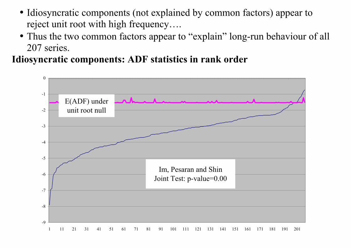
• Idiosyncratic components (not explained by common factors) appear to reject unit root with high frequency….

• Thus the two common factors appear to “explain” long-run behaviour of all 207 series.

Idiosyncratic components: ADF statistics in rank order

-9

-8

-7

-6

-5

-4

-3

-2

-1

0

1 11 21 31 41 51 61 71 81 91 101 111 121 131 141 151 161 171 181 191 201

E(ADF) under unit root null

Im, Pesaran and ShinJoint Test: p-value=0.00

Principal Components from Differenced Output • Trend growth captured by mean growth rates • First 3 PCs roughly V-shaped, but a messier picture. We focus on levels

results.

-40

-30

-20

-10

0

10

1975 1980 1985 1990 1995 2000

ALLSECTORSPC1ALLSECTORSPC2-ALLSECTORSPC3

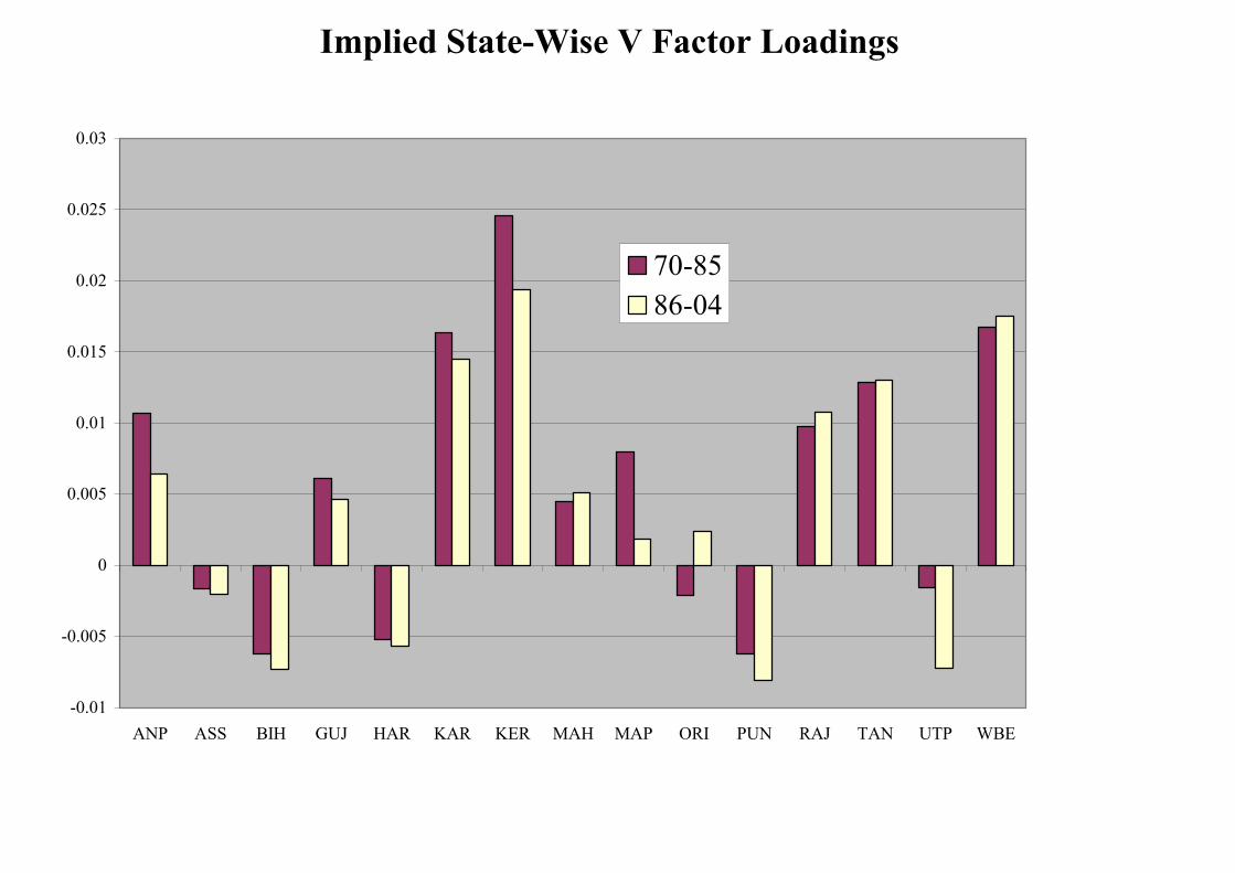
Implied State-Wise V Factor Loadings

-0.01

-0.005

0

0.005

0.01

0.015

0.02

0.025

0.03

ANP ASS BIH GUJ HAR KAR KER MAH MAP ORI PUN RAJ TAN UTP WBE

70-8586-04

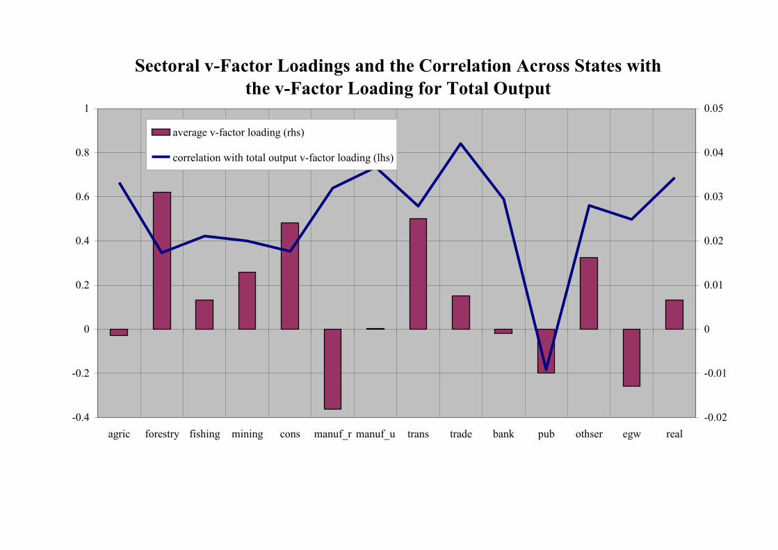
Sectoral v-Factor Loadings and the Correlation Across States with the v-Factor Loading for Total Output

-0.4

-0.2

0

0.2

0.4

0.6

0.8

1

agric forestry fishing mining cons manuf_r manuf_u trans trade bank pub othser egw real-0.02

-0.01

0

0.01

0.02

0.03

0.04

0.05

average v-factor loading (rhs)

correlation with total output v-factor loading (lhs)

Sectoral V-Factor Loadings

Compares the sum of the factor loadings on the V-factor for all 14 sectors in each state with those for output as a whole.

Did Breaking States Differ in Initial/Other Characteristics?

Values in 1987

• Regression Analysis: Dependent Variable is the change in the average log growth rate across 1970-1987 and 1987-2004

• Most significant individual effect is the negative impact of the sectoral share of agriculture in any given state.

• Means that a state that was predominantly agricultural was in itself an

obstacle to the state’s participation in the turnaround in growth across all sectors.

• A higher literacy rate plays a similar role.

• Land-locked states less able to have been able to participate in the

turnaround.

Other Observations

• Average factor loading on registered manufacturing negative.

• Results support Aghion et al (2008): more pro-worker states less likely to benefit from the reforms.

• Solow variables did not have any explanatory power

• (Only a few) non – trade indicators line up with the V factor.

Timing of the V-factor fits timing of trade policy shift pretty well (Rodrik & Subramanian, 2005)

-8

-6

-4

-2

0

2

4

6

8

1970

1972

1974

1976

1978

1980

1982

1984

1986

1988

1990

1992

1994

1996

1998

2000

2002

2004

2006

0.00

10.00

20.00

30.00

40.00

50.00

60.00

70.00

v-factorduties/imports

Other Indicators

0

10

20

30

40

50

60

70

1970 1975 1980 1985 1990 1995 2000 20050

0.5

1

1.5

2

2.5

3

3.5

4

4.5

Duties As Percentage of Imports Duties As Percentage of GDP (right-hand scale)

Log of Openness Ratio

0.8

0.9

1

1.1

1.2

1.3

1.4

1.5

1.6

1970 1975 1980 1985 1990 1995 2000 2005

Log of Openness Ratio

Robustness

• Use longer datasets despite a reduction in the cross-section dimension.

• Leads to an identical timing of the apex with similar paths afterwards. • We then exclude data on the basis of state characteristics, broad industry

type, high volatility, and adjusting for fluctuations in rainfall. • Broad profile of V-factor very similar.

• Simulations (simulate each of the N series as a sum of the factor loadings

on two I(1) factors plus a persistent residual component)

Conclusions

• We find a common “V-factor” that explains growth shifts across states and

sectors. Timing – mid to late eighties.

• We see signs of a break in growth in the mid- to late ‘80s, somewhat later than, e.g. Rodrik & Subramanian (2005). Registered manufacturing not the channel.

• Factor loadings are differentèbreak is not universal to all states.

• Literacy rates, agriculture/NSDP, “land-lockedness”, pro-employer institutions, have a significant relation with V-factor loadings.

• “V-states” are not richer; nor are Solow variables the explanation.

• The V-Factor appears strongly inversely correlated with several measures of trade liberalisation.