NBER WORKING PAPER SERIES

THE EFFECT OF NATURAL DISASTERS ON ECONOMIC ACTIVITY IN US COUNTIES: A CENTURY OF DATA

Leah Platt BoustanMatthew E. KahnPaul W. Rhode

Maria Lucia Yanguas

Working Paper 23410http://www.nber.org/papers/w23410

NATIONAL BUREAU OF ECONOMIC RESEARCH1050 Massachusetts Avenue

Cambridge, MA 02138May 2017

The views expressed herein are those of the authors and do not necessarily reflect the views of the National Bureau of Economic Research. Paul Rhode acknowledges the support of the Michigan Institute for Teaching and Research in Economics.

NBER working papers are circulated for discussion and comment purposes. They have not been peer-reviewed or been subject to the review by the NBER Board of Directors that accompanies official NBER publications.

© 2017 by Leah Platt Boustan, Matthew E. Kahn, Paul W. Rhode, and Maria Lucia Yanguas. All rights reserved. Short sections of text, not to exceed two paragraphs, may be quoted without explicit permission provided that full credit, including © notice, is given to the source.

The Effect of Natural Disasters on Economic Activity in US Counties: A Century of DataLeah Platt Boustan, Matthew E. Kahn, Paul W. Rhode, and Maria Lucia YanguasNBER Working Paper No. 23410May 2017JEL No. N42,Q5,R23

ABSTRACT

Major natural disasters such as Hurricanes Katrina and Sandy cause numerous fatalities, and destroy property and infrastructure. In any year, the U.S experiences dozens of smaller natural disasters as well. We construct a 90 year panel data set that includes the universe of natural disasters in the United States from 1920 to 2010. By exploiting spatial and temporal variation, we study how these shocks affected migration rates, home prices and local poverty rates. The most severe disasters increase out migration rates and lower housing prices, especially in areas at particular risk of disaster activity, but milder disasters have little effect.

Leah Platt BoustanPrinceton UniversityIndustrial Relations SectionLouis A. Simpson International Bldg.Princeton, NJ 08544and NBERlboustan@princeton.edu

Matthew E. KahnDepartment of EconomicsUniversity of Southern CaliforniaKAPLos Angeles, CA 90089and NBERkahnme@usc.edu

Paul W. RhodeEconomics DepartmentUniversity of Michigan205 Lorch Hall611 Tappan St.Ann Arbor, MI 48109-1220and NBERpwrhode@umich.edu

Maria Lucia YanguasDepartment of EconomicsUCLALos Angelesmyanguas@ucla.edu

An online appendix is available at http://www.nber.org/data-appendix/w23410

2

I. Introduction

Major natural disasters such as Hurricanes Andrew, Katrina and Sandy cause numerous

fatalities, and destroy private property and public infrastructure. As more economic activity

clusters along America’s coasts, the population is now at greater risk of exposure to natural

disasters (Changnon et. al. 2000, Rappaport and Sachs 2003, Pielke et. al. 2005). Furthermore,

climate science suggests that, as global greenhouse gas emissions increase, so too will the

quantity and severity of certain types of natural disasters (IPCC 2012). This heightened disaster

risk highlights the importance of having a better understanding of how natural disasters affect the

economy.

In this paper, we study the universe of natural disasters in the United States from 1920 to

2010, from the most severe to the comparatively mild. By studying the full spectrum of such

events, we can examine responses to both the quantity and intensity of natural disasters at the

local level. Our unit of analysis is a US county. We assess whether counties that faced disasters

lost population through net out-migration and experienced rising poverty rates, perhaps because

of selective out-migration of the non-poor. We also ask whether population outflows were

accompanied by falling housing prices and rents.

With access to disaster counts for almost a century, we are able to include a rich set of

controls, including county fixed effects and state-specific time trends, which absorbs many

attributes of disaster-prone areas on the coasts or in the flood plain of large rivers. We also

control directly for changes in local labor demand by predicting employment growth using a

county’s baseline industrial structure interacted with national growth trends (the standard Bartik

measure).

3

One of our paper’s empirical contributions is to create a new long-run disaster data base

at the county level in the United States spanning from 1920 to 2010. We combine data from the

American Red Cross (ARC, 1920-64) and the Federal Emergency Management Agency and its

predecessors (FEMA, 1950-2010). The mean county in our dataset faced two disasters in a

typical decade, with floods being the most common event type followed by storms and

hurricanes. In each decade, one in three counties experienced a severe disaster (with 10 or more

deaths) and one in ten counties experienced a super-severe disaster (with 100 or more deaths).

We find that a one standard deviation increase in disaster count (2.4 disasters) heightens

the out-migration rate from a county by 1 percentage point (5 percent of a standard deviation).

The strongest migration response is to volcanos, hurricanes and forest fires. The effect of one

super-severe disaster is twice as large as the response to the average disaster. The migration

response to the most severe natural disasters is on the same order of magnitude as the effect of a

one standard deviation increase in predicted employment growth. Poverty rates also increase in

areas hit by super-severe disasters, which is consistent with out-migration of the non-poor, in-

migration of the poor (perhaps in response to lower housing prices), or a transition of the existing

population into poverty.

The migration response to disasters varies over the century and across locations. Of

particular interest is how the 1978 advent of FEMA, which coordinated the federal response to

natural disasters, may have influenced the likelihood of out-migration following a disaster event.

One might expect that residents would be less likely to move out of disaster-struck areas after the

creation of FEMA, if FEMA increased payments of federal disaster relief. This “moral hazard”

effect has been extensively discussed in the popular media and has been the topic of some

academic study (e.g., Gregory, 2014). Yet, we find that, if anything, out-flows in response to

4

natural disasters were higher in recent decades, despite the advent of FEMA, perhaps because

disaster events have been worsening in frequency over time. This pattern is also consistent with

Deryugina’s (2016) observation that transfer payments following disasters come mainly in the

form of unemployment insurance and other non-place-based programs. It appears that many

people in disaster affected areas take the money and move to another county.

Due to exogenous variation in geography, topography and climate conditions, counties

differ with respect to their risk of natural disaster events. For example, coastal areas or areas in

the flood plain of a river are more at risk of experiencing a natural disaster, whereas areas at

higher elevation are at lower risk. We test whether migration rates are more responsive to

disasters in areas that are less prone to experience them. One theory is that natural disasters have

higher salience in “low risk” areas and residents are caught off guard when experiencing a shock

that they were not prepared for. An alternative theory posits that since migration is a long run

investment, it makes sense to migrate away from areas that have been shocked if such shocks are

expected to be persistent over time. A forward-looking migrant will recognize that such areas are

likely to suffer again and thus the long run present discounted value of benefits of remaining

there is lower (Sjaastad 1962). Consistent with the second view, we find that net outmigration

rates are higher in areas that are prone to suffer disasters when such areas experience a very

severe shock.

Our work contributes to two strands of the climate and environmental economics

literatures. First is a series of macroeconomic studies that use cross-country panel regressions to

study how changing temperature, rainfall, and increased exposure to natural disasters conditions

affects economic growth (Dell, Jones and Olken 2012, 2014; Cavallo, Galiani and Pantano 2013;

Anttila-Hughes and Hsiang 2013; Hsiang and Jina 2014; Burke, Hsiang and Miguel 2015;

5

Kocornik-Mina et. al., 2015). By analyzing the effect of natural disasters in a single country over

many decades, we are able to hold constant many core institutional and geographic features of

the economy that may be correlated with disaster prevalence in a cross-country setting (e.g.,

democracy, temperate climate). The closest paper to ours in this respect is Strobl (2011), which

uses a county-level panel of coastal US counties to study how hurricanes affected local economic

growth during the years 1970 to 2005. A second set of papers uses case studies of specific major

disasters to examine how shocks to a geographic area affect existing residents (see, for example,

Smith and McCarty 1996 on Hurricane Andrew; Hornbeck 2012 and Long and Siu 2016 on the

Dustbowl; Hornbeck and Naidu 2014 on the 1927 Mississippi flood; and Vigdor 2008 and

Deryugina, Kawano and Levitt 2014 on Hurricane Katrina; Frankenberg et. al. 2011 examine the

consequences of the Indian Ocean tsunami). While it is important to study these major cases,

most disasters are not as severe as these notable outliers. Our data collection allows us to

examine a much larger set of disasters, which includes – but is not limited to – some of the major

disasters listed above.

Throughout this paper, we view local labor demand shifts and natural disasters as shocks

to the underlying spatial equilibrium. We thus start by discussing an augmented Rosen/Roback

spatial equilibrium model to introduce such shocks. We then present our estimating equation and

core hypotheses, our data and our main results.

6

II. Natural Disaster Risk in a Static Spatial Equilibrium Model

In the simplest version of the spatial equilibrium model, all people have the same

preferences over private consumption and local public goods and face zero migration costs

(Roback 1982). Geographic areas differ by one exogenous attribute such as winter temperature.

From this local variation, a hedonic rental price equilibrium arises mapping out the

representative agent’s indifference curve between private consumption and (say) outdoor

temperature. There is no migration in equilibrium because utility is equalized across all

locations. Residents of colder places are compensated in the form of lower rents.

Now suppose that counties are at risk of experiencing two types of shocks: shifts in local

labor market demand and the occurrence of natural disasters. In each decade, some counties

enjoy an increase in local labor demand, while others face declining local labor demand.

Furthermore, some counties experience a natural disaster, while others do not.

An increase in local labor market demand will lower unemployment risk and raise local

wages. This positive shock should attract migrants to the area (Topel 1986). In contrast, the

occurrence of a natural disaster will decrease the local amenity level – for example, by imposing

some extra mortality risk. All else equal, such natural disasters should push people to leave and

discourage outsiders from moving in. In an economy featuring durable local housing, the

housing supply will be inelastic and this means that a downward shock to local quality of life

will depress local home prices (Glaeser and Gyourko 2005). Lower home prices act to anchor the

poor as their real purchasing power increases as rents decline. We thus predict that areas that are

routinely hit by natural disasters will experience out migration but such migration will be slowed

7

down by declining home prices and this will shift the area’s composition such that a larger share

of the residents are poor.

III. Econometric Framework

In our main regression specifications, we study how economic activity changes in response to

the quantity and severity of natural disasters. Our unit of analysis will be a county/decade and the

data will cover the decades 1930 to 2010. We measure economic activity using dependent

variables such as a county’s net migration rate, poverty rates and home prices/rents. A second set

of results then tests for heterogeneous responses to natural disasters. For example, we test if high

amenity or high productivity places experience more/less negative effects when disasters occur.

We further explore whether the effects of disasters differ by disaster category (floods, hurricanes,

etc.) and whether these relationships are stable over time.

Our main specification is an unweighted regression, in which each county contributes equally

to the estimation. This approach considers each county to be a separate place that may be subject

to a location-specific shock in a given period. Our interest then is in observing how these places

are affected by (and potentially recover from) local shocks. In this way, our main specification

corresponds to the cross-country regressions common to the climate economics literature. For

completeness, we also present results weighted by a county’s population in the year 1930 (see

Web Appendix). This specification puts more weight on disasters that take place in heavily

populated urban areas.

8

Define county i in State Economic Area (SEA) z in state j in decade t. Our core

econometric results will be based on estimating equation (1).1

μ ∗ ∗ ∗ (1)

In this equation, Y represents a set of dependent variables that includes a county’s

migration rate, housing prices/rents, and the poverty rate. We include county and decade fixed

effects and state specific time trends. Disasters is a vector of the quantity and severity of

disasters in a local area. We discuss this vector in depth after we introduce our disaster data. The

variable ‘Bartik’ is an estimate of employment growth in county i during the period t-10 to t

using initial industrial composition to weight national employment trends. This is the standard

proxy for exogenous shifts in local labor demand introduced by Bartik (1991) and Blanchard and

Katz (1992). This variable’s construction is presented in equation (2). U is the error term and it is

clustered at the county group (SEA) level. We report results collapsed to the SEA level in the

Web Appendix.

∑ , , ∗ ,

, (2)

Equation (2) provides the formula for our Bartik measure. We weight the national growth

rate (NGR) in employment in industry l for decade t by the share of people in county i who

worked in this industry in the base year (1930).

                                                            1 SEAs are either single counties or groups of contiguous counties within the same state that had similar economic characteristics when they were originally defined, just prior to the 1950 census (Bogue, 1951). https://usa.ipums.org/usa-action/variables/SEA#description_section.

9

IV. Data

Natural Disasters

Creating a consistent data set of natural disasters at the county level over the twentieth

and the early twenty-first centuries requires combining data from several sources. The list of

“major disaster declarations” posted by FEMA and its predecessors begins in 1964

(https://www.fema.gov/disasters). We supplement the FEMA roster with information published

in the Federal Register back to 1958 and with archival records back to 1950s.2 For each disaster,

we recover the geographic location (county), disaster type, and month and year of occurrence.

We expand our coverage back to 1918 by using data from the disaster relief efforts of the

American National Red Cross (ARC). These efforts are documented in their Annual Reports and

in various versions of the ARC’s “"List of Disaster Relief Operations by Appropriation

Number,”, held in Record Group 200 at the National Archives in College Park, MD.3 We link

these lists with the ARC’s case files to document the date, type, and location of each disaster.4

We identify the larger-scale disasters using the ARC’s Circulars, which were published from the

early 1920s on whenever the ARC engaged in major relief efforts.

Our dataset includes the following set of natural disasters: floods (including tidal waves),

storms, hurricanes, tornadoes, earthquakes, volcanic eruptions, droughts and other natural

disasters such as forest fires, extreme temperatures and landslides. All human-related disasters

                                                            2 Specifically, we use the archival records of the Office of Emergency Preparedness (Record Group 396) and of the Office of Civil and Defense Mobilization, the Office of Defense and Civil Mobilization, and the Federal Civil Defense Administration i (Record Group 397) held in the National Archives at College Park, Maryland. The “State Disaster Files” in RG 396, Boxes 1-4 were especially used. 3 See Record Group 200, Records of the American National Red Cross, 1947-1960, Boxes 1635-37, held in the National Archives at College Park, Maryland 4 The case files are located in RG200 Records of the American National Red Cross, 1917-34, Box 690-820; 1935-46, Boxes 1230-1309; 1947-60, Boxes 1670-1750.

10

such as mine collapses, explosions, transportation accidents and arsons are excluded from the

analysis.

In addition to counting the number of declared disasters in an area, we also rank disasters

by fatalities, one measure of their intensity. Death counts for most severe disasters in the United

States are available from EM-DAT, the International Disaster Database, which was created by

the Centre for Research on the Epidemiology of Disasters (CRED). (See http://www.emdat.be/

for details.) The EM-DAT lists the date, type, location, and death tolls of all major natural

disasters over the twentieth and twenty-first centuries.5 Although EM-DAT has coverage back to

1900, its historical data is less comprehensive. We supplement EM-DAT with information on

death counts from the American Red Cross for earlier years.

With these data in hand, we create four measures of the frequency and intensity of

disasters in a county/decade. We start by simply counting the number of declared disasters in an

area. We then include two indicators of disaster intensity, the first equal to one if a natural

disaster led to ten or more deaths (“severe”) and the second equal to one if the disaster resulted in

100 or more deaths (“super-severe”). Finally, we code a dummy variable equal to one if the

county experienced any disasters in a decade. We observe that sparsely populated places have

few recorded disasters (see, for example, the Mountain West in Figure 2), presumably because

disaster declarations are based not only on the severity of a storm but also on the number of

people likely affected. This indicator is an important control given that there was net migration

away from these unpopulated places over time.

                                                            5 To be included in EM-DAT, disasters must fit at least one of the following criteria: ten or more reported deaths, one hundred or more people reported affected, declaration of a state of emergency, or call for international assistance.

11

Figure 1 displays annual counts of disaster events at the disaster-by-county level from

1920-2010. By this measure, a disaster that affects multiple counties would be tallied multiple

times, and a county that is struck by more than one disaster in a given year would also count

more than once. The first half of the time series records data from the American Red Cross

(1920-64), while the second half includes data from FEMA and its predecessors. From 1920-

1980, around 500 separate county-disaster events took place in a given year. From 1980 to the

present, and especially after the early 1990s, there has been a clear acceleration in disaster

counts, reaching around 1,500 county-level events per year by the 2000s.

Our reading of the evidence is that some of this acceleration is capturing a real increase in

the underlying frequency of storms. An uptick in disaster events is evident in comparable global

series as well, suggesting that we are not merely picking up a change in US government policy

toward disaster relief (see Munich Re, 2012; Gaiha, et al., 2013; Kousky 2014). Yet, we also

suspect that the federal government became more expansive in the declaration of disaster events

after Hurricane Andrew, which was notably destructive and especially salient, given that it took

place during the 1992 presidential election campaign (Salkowe and Chakraborty 2009). Political

science research has investigated the determinants of FEMA disaster declarations. Garrett and

Sobel (2003) and Downton and Pielke (2001) find that the president and Congress affect the rate

of disaster declaration and the allocation of FEMA disaster expenditures across states. States

politically important to the president have a higher rate of disaster declaration, and disaster

expenditures are higher in states having congressional representation on FEMA oversight

committees and during election years. Garrett and Sobel suggest that nearly half of all disaster

relief is motivated politically rather than by need.

12

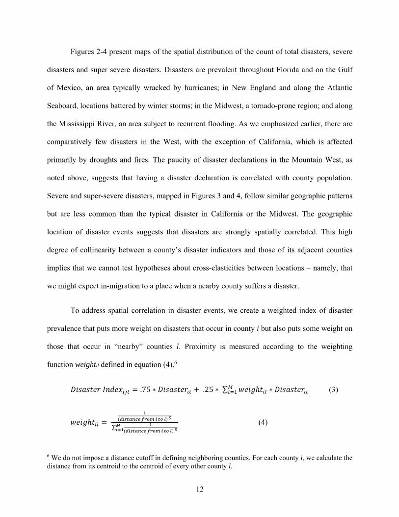
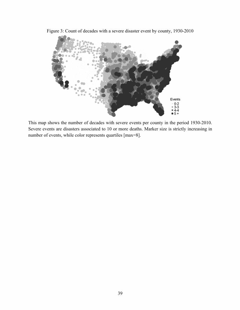
Figures 2-4 present maps of the spatial distribution of the count of total disasters, severe

disasters and super severe disasters. Disasters are prevalent throughout Florida and on the Gulf

of Mexico, an area typically wracked by hurricanes; in New England and along the Atlantic

Seaboard, locations battered by winter storms; in the Midwest, a tornado-prone region; and along

the Mississippi River, an area subject to recurrent flooding. As we emphasized earlier, there are

comparatively few disasters in the West, with the exception of California, which is affected

primarily by droughts and fires. The paucity of disaster declarations in the Mountain West, as

noted above, suggests that having a disaster declaration is correlated with county population.

Severe and super-severe disasters, mapped in Figures 3 and 4, follow similar geographic patterns

but are less common than the typical disaster in California or the Midwest. The geographic

location of disaster events suggests that disasters are strongly spatially correlated. This high

degree of collinearity between a county’s disaster indicators and those of its adjacent counties

implies that we cannot test hypotheses about cross-elasticities between locations – namely, that

we might expect in-migration to a place when a nearby county suffers a disaster.

To address spatial correlation in disaster events, we create a weighted index of disaster

prevalence that puts more weight on disasters that occur in county i but also puts some weight on

those that occur in “nearby” counties l. Proximity is measured according to the weighting

function weightil defined in equation (4).6

.75 ∗ .25 ∗ ∑ ∗ (3)

.

∑ .

(4)

                                                            6 We do not impose a distance cutoff in defining neighboring counties. For each county i, we calculate the distance from its centroid to the centroid of every other county l.

13

The weights in equation (4) add up to one and the resulting index in equation (3) varies

between 0 and 1. An index value equal to zero means that neither the county itself nor its

neighbors experienced a natural disaster in that decade. The Web Appendix reports results based

only on the count of disasters occurring in own county i. We follow the procedure described

above for each of our disaster variables.

Migration

We obtain age-specific net migration estimates for US counties from 1950-2010 from the

University of Wisconsin-Madison and from 1930-50 through ICPSR. These data include

estimates of net migration for each decade from US counties by five-year age group, sex, and

race. The underlying migration numbers are estimated by comparing the population in each age-

sex-race cohort at the beginning and end of a Census period (say, 1990-2000) and attributing the

difference in population count to net migration, after adjusting for likely mortality. This method

has become standard practice to estimate internal migration in the United States, as originated by

Kuznets and Thomas (1957). We divide estimated net migration to or from the county from time

t to t+10 by population at time t to calculate a migration rate.

Other Data

The county-by-decade prediction of employment growth in equation (2) is constructed by

first calculating employment shares by industry in a base year (1930), and then using these share

to weight national rates of employment growth by industry and decade. Our measure relies on

individual data on employment in 143 industries in the IPUMS dataset using the standardized

1950-based industries codes. We also use data on poverty rates and house values/rents (1960-

2000/1970-2010) by county from NHGIS. The geography variables used in our prediction of

14

local disaster risk, such as elevation and distance to the coast, are from Fishback et. al. (2006).

We classify counties into “good” and “bad” weather areas (our measure of local amenities) using

an index comparing average January and July temperatures from NOAA.7

V. Results

We begin in Table 1 by reporting summary statistics for our sample of nearly 25,000

county-by-decade level observations. The typical county in our sample had 1.97 declared

disasters in a decade, with the most common disasters being storms (0.79), floods (0.49) and

hurricanes (0.31). Three out of ten counties experience a severe disaster, while one out of ten

experience a super-severe disaster. One percent of the population, or around 2,000 residents, left

the average county in a decade, but there is substantial variation around this mean. Table 1 also

reports summary statistics for poverty rate and housing values.

Each local disaster declaration is associated with a small increase in net out-migration at

the county level, with a substantially larger effect of super-severe disasters. Table 2 reports our

main estimates of equation (1). Each declared disaster increases net out-migration by 0.5

percentage points (2.5 percent of a standard deviation). There is no additional effect on out-

migration if a disaster is considered severe (10 or more deaths). But a super-severe disaster (100

or more deaths) has a much larger effect on population loss, increasing net out-migration by

almost 3 percentage points (15 percent of a standard deviation).8 For comparison, our estimates

                                                            7 Our good weather index is: [mean average daily January temperature/standard deviation – mean average daily July temperature/standard deviation]. We classify counties as being “good weather” areas if their index value is above the median. 8 We also control for an indicator equal to one in counties that faced at least one disaster in the decade. We find net in-migration to counties that had at least one declared disasters, perhaps counties with no

15

suggest that a one standard deviation decline in the estimated employment growth in a county

would increase out-migration by 3 percentage points (= -0.12 x 0.276). Experiencing one super-

severe disaster is as disruptive to a local population as a large negative employment shock. The

Web Appendix reports results for the subsample of young men, who tend to be more mobile, and

implied effects (in standard deviation terms) are similar.

We note that our estimates are net effects of a disaster on migration activity after all

private and government responses to the disaster event take place (e.g., infrastructure investment,

transfer payments). A disaster at the start of a given decade may trigger infrastructure

investments in flood control or early warning systems that mitigate future risk. New investments

may attract people to an area both because of declines in natural disaster risk and because of

short run jobs stimulus. Our results are unchanged by controlling for new dam construction in the

decade, the largest of such infrastructure projects (see Web Appendix).9

Changing Migration Response to Disaster Events over Time

From the 1920s through the 1950s, the federal government responded to natural disasters

on a case-by-case basis. In the 1950s, the federal government assumed a more systematic disaster

relief role through a succession of Civil Defense agencies. During the 1970s, Washington

coordinated its response to disaster events, first by creating the Federal Disaster Assistance

Administration in 1973 under the Department of Housing and Urban Development and then by

                                                                                                                                                                                                disasters tended to be sparsely populated and population has been moving away from rural areas over time. Excluding this indicator does not affect the coefficient on super-severe disasters, but does bias the coefficient on disaster count toward zero. 9 Duflo and Pande (2005) study the productivity and distributional effects of large irrigation dams in India. They find that rural poverty declines in downstream districts but increases in the district where the dam is built.

16

creating an independent agency, the Federal Emergency Management Agency (FEMA) in 1978.

In Table 3, we test for a difference in the migration response to disaster events that occur before

and after these policy changes. If FEMA increased the federal disaster relief available in a

county, we might expect the net out-migration to decline as residents are anchored to an area by

receipt of federal funds. However, we note that the intensity of disaster activity increased over

time, especially after 1990, in part due to environmental change (Figure 1), and so it is hard to

disentangle the effects of policy change from the environment.

Table 3 documents that there was little migration response to disasters before 1980. The

main results for the century presented in Table 2 are primarily picking up the heightened out-

migration response to disaster events after 1980. In this period, each disaster increased net out-

migration from a county by 1 percentage point, although this outflow was mitigated in the case

of severe disasters. Each super-severe disaster increased out-migration by 4 percentage points.

Any drag on migration from the establishment of FEMA was swamped by changes in the nature

of disasters, which may be becoming more damaging or more salient to households over time.

Our finding that the establishment of FEMA did not anchor residents in place is

consistent with Deryugina (2011), which documents that counties struck by hurricanes in the

1980s and 1990s received around $1,000 (2008 dollars) per capita in additional federal transfers

in the decade after a hurricane event. Two-thirds of these funds were dispersed through

unemployment insurance and income maintenance programs that are not tied to the recipient’s

location. The population in disaster-struck areas can move elsewhere and continue to receive

income support.

17

Heterogeneous Migration Responses to Disaster Events

Low Risk vs. High Risk Areas

The remainder of the paper explores heterogeneous responses to disaster events by

disaster risk, disaster type, urban status, amenity level and racial composition. We start by

considering whether disasters have a differential effect on economic outcomes in areas that face

higher disaster risk given their local geography and climate. We create a propensity score

measuring the likelihood that county i suffers a severe natural disaster in decade t. In particular,

we estimate a linear probability model using exogenous geographical and topographical

attributes included in the vector Z and use this regression to predict the county-specific

propensity score . 10

μ ∗ (5)

In Table 4, we interact this regressor with the indicators for severe and super-severe

disasters. Recall that the level of p(Z) is captured by the county fixed effects. We find evidence

of greater out migration from areas that suffer extreme natural disasters (either severe or super-

severe) if these areas are at a higher propensity for disaster events. This pattern suggests that

migrants respond more to a given shock in areas with geography prone to such shocks, such as

low elevation areas on a coastline or in a river plain. This pattern might arise because current

shocks are more likely to predict future shocks in areas that are prone to disaster activity. We do

not find evidence consistent with the idea that residents of high-risk areas anticipate such events

                                                            10 In the Web Appendix, we present the first stage regression for creating the propensity score. The major predictors of a severe disaster are proximity to a coast or a river, or being at low elevation.

18

and thus invest in effective disaster prevention, such as moving out of mobile homes or retro-

fitting their house for earthquake safety (see, for example, Lim, 2016 on tornadoes).

Productive Places and Areas with High Amenity Levels

Areas with strong productivity fundamentals should be more easily able to rebound from

natural disasters than local economies that are otherwise waning. During the twentieth century,

urban and metropolitan areas were gaining population and economic activity at the expense of

rural areas. We thus expect that natural disasters that hit these less-productive rural counties may

have larger effects on the net out-migration rate than similar disasters that strike more populated

counties.

We construct two definitions of urban/metropolitan counties to apply throughout the

century. The first definition contains all counties that were part of a metropolitan statistical area

in 1970. The second definition instead includes all counties with a population density greater

than the national median in 1930.

We find that the effect of disaster events on net out-migration is two to three times as

large in rural counties than in their urban counterparts. Table 5 reports results that split the

sample according to the first definition; a similar table using the second definition is included in

the Web Appendix. This finding is consistent with Feng, Oppenheimer and Schlenker (2012)

who find significant out-migration from rural counties in the Corn Belt following climate-driven

drops in crop yields and with Cattaneo and Peri (2015), who find that higher temperatures due to

global warming increase emigration rates from rural to urban areas in middle income economies.

Following the same logic, we expect less outflow in response to a given natural disaster

that strikes an area that is otherwise attracting population due to high levels of local amenities.

19

One local amenity that unambiguously attracted population over the twentieth century was

pleasant weather (Gyourko and Tracy, 1991; Gyourko, Kahn and Tracy, 1999). Table 6 splits the

sample into counties that are above and below the median on a “good weather” index. We find

no significant difference in the response to severe or super-severe disasters by local climate. If

anything, and contrary to our reasoning, it appears that residents are more likely to move away

from good weather areas for a given number of mild disaster events. However, this differential

responsiveness to mild disasters is driven by the composition of disaster types in good and bad

weather areas. Good weather counties are more likely to face hurricanes and disasters in the

“other” category (landslides, forest fires), which have the strongest effect on out-migration (see

Table 8 below). The Web Appendix includes a version of Table 6 that separately controls for

event counts by disaster type.

Blacks vs. Whites

In the early twentieth century, the majority of blacks lived in the rural South, many in the

flood plain of the Mississippi River. More than half of southern blacks moved to other regions,

particularly in the years 1940 through 1970 (Boustan, 2017). Hornbeck and Naidu (2014)

examine the impact of the Great Mississippi Flood of 1927 and find that flooded counties

experienced an immediate and persistent out-migration of black population. However, it is hard

to draw inferences on black migration response to natural disasters from one extreme event

alone. In Table 7, we report results separately for whites and blacks. Although the coefficients

are not individually statistically significant, it appears that the black migration response to total

disaster count and to extreme disaster events is substantially larger than the white response.

20

Disaster Category

Certain disaster types have much stronger effects on out-migration than others. In Table

8, we break out the disaster count variable by category. The overall effect of disasters on

migration activity – a 0.5 percentage point increase in net out-migration – is a weighted average

of more and less destructive disaster types. The migration response is strongest to volcanic

eruptions, hurricanes, and the “other” disaster category, which includes forest fires and

landslides. Storms also encourage net out-migration. On the other hand, and surprisingly,

tornados and earthquakes appear to have no effect on mobility flows, and floods actually

encourage some net in-migration. The pattern for floods is consistent with our earlier work, in

which we found that migrants moved toward counties that experienced floods in the 1920s and

1930s (Boustan, Kahn and Rhode, 2012). We posited that areas prone to flooding received new

infrastructure in this period, which may have encouraged new use of previously marginal land.

However, it appears that in-migration to flooded areas continued throughout the century.

Furthermore, the positive effect of flooding on in-migration is present even when we control for

the construction of new dams during the decade. We also note that migrants are very strongly

attracted to areas experiencing drought. Drought are associated with low precipitation and

higher-than-average temperatures, two amenities that attract residents (even if they may be

detrimental for local agriculture).

Measuring the Impact of Disasters on Home Prices and Poverty Rates

If natural disasters encourage net out-migration from a county, lowering demand for the

area, we would expect an associated effect of disaster activity on housing prices and rents (see

21

Hallstrom and Smith 2005). In rare cases, disasters also destroy a substantial portion of the

housing stock, in which case the effect on housing prices would be ambiguous. The first two

columns of Table 9 analyze the effect of disasters on median housing values and monthly rents in

a county. The total number of declared disasters has no effect on local housing prices and rents,

despite encouraging a mild amount of net out-migration. Yet, the occurrence of a super-severe

disaster lowers housing prices by 6 percent and rents by 3 percent. The implied elasticity of

housing prices with respect to population loss – a 3 percent decline in rents for out-migration

representing 2 percent of the population – is similar to standard estimates in the literature (e.g.,

Saiz, 2007, which looks at the effect of foreign in-migration on rents).

Residents who leave an area after a natural disaster may represent a select subsample of

the incumbent population. We suspect that rich households would have greater resources to leave

an area struck by disaster. In the climate change adaptation literature, there is a broad consensus

that the wealthy can access a wide range of protective strategies ranging from owning a second

home, to accessing better quality medicine, food and medical care and housing to protecting

themselves from shocks; the poor are thus more likely to bear the incidence of natural disasters

(Dasgupta 2001; Barreca, et. al. 2016; and Smith et. al. 2006.). If the rich are more likely to leave

an area after a disaster, net out-migration may serve to increase the local poverty rate. We test

this hypothesis in the third column of Table 9. While each declared disaster slightly reduces area

poverty, the occurrence of a super-severe disaster increases the local poverty rate by 1.1

percentage points (13 percent of a standard deviation).

22

VI. Conclusion

During the past century, the United States has experienced more than 5,000 natural

disasters. Some have been major newsworthy events, while others have been comparatively

mild. We compile a near-century long series on natural disasters in US counties, distinguishing

severe events by death toll, and find that these shocks affect the underlying spatial distribution of

economic activity.

Counties hit by severe disasters experienced greater out-migration, lower home prices

and higher poverty rates. Given the durability of the housing capital stock, lower demand to live

in an area due to persistent natural disasters leads to falling rents and acts as a poverty magnet.

This dynamic is particularly apparent in areas that face high disaster risk or that lack other

productivity advantages. Glaeser and Gyourko (2005) documented a similar spiral in declining

cities (i.e., Detroit). In their setting, the cause of declining housing demand was a persistent

decline in local labor demand following the contraction of the US auto industry.

Our estimate of the average effect of super-severe disasters (those with 100 or more

deaths) on out-migration is much lower than estimates arising from case studies of the nation’s

most extreme events. We find a 3 percentage point increase in net out-migration in disaster

struck counties, which is substantially lower than the 12 point increase in out-migration from

New Orleans after Hurricane Katrina (Deryugina, et al., 2014); the 12 point increase in the out-

migration rate from flooded counties in the 1927 flood (Hornbeck and Naidu, 2014); and a 12

percent reduction in the population of counties facing high erosion during the Dustbowl

(Hornbeck 2012; Long and Siu 2016).

23

In recent years, two independent literatures have emerged studying the population

responses to large local shocks, including natural disasters and war-time bombing. Population

appears to quickly recover after an area is bombed (Davis and Weinstein 2002; Brakman,

Garretsen and Schramm 2004; Miguel and Roland 2011, but see also Schumann, 2014). Yet war

and natural disasters differ in their expected persistence. Coastal areas and flood plains are

shocked again and again by natural disasters, whereas, in the case of war, the shocks end with a

peace treaty and investors can invest with confidence. The expectation of future shocks in areas

hit by natural disasters raises the likelihood of disinvestment both in terms of labor and capital

from such increasingly vulnerable areas. Whether the federal government seeks to counter such a

trend through local stimulus, and what are the equilibrium impacts on labor and capital flows

remains an open question.

24

VII. References

Anttila-Hughes, J. K., & Hsiang, S. M. (2013). Destruction, disinvestment, and death: Economic and human losses following environmental disaster.

Barreca, A., Clay, K., Deschenes, O., Greenstone, M., & Shapiro, J. S. (2016). Adapting to climate change: The remarkable decline in the US temperature-mortality relationship over the twentieth century. Journal of Political Economy, 124(1), 105-159.

Bartik, T. J. (1991). Boon or boondoggle? The debate over state and local economic development policies.

Blanchard, O. J., Katz, L. F., Hall, R. E., & Eichengreen, B. (1992). Regional evolutions. Brookings papers on economic activity, 1992(1), 1-75.

Boustan, L. P., Kahn, M. E., & Rhode, P. W. (2012). Moving to higher ground: Migration response to natural disasters in the early twentieth century. American Economic Review, 102(3), 238-244.

Boustan, L. P. (2017). Competition in the Promised Land: Black migrants in northern cities and labor markets. Princeton: Princeton University Press.

Brakman, S., Garretsen, H., & Schramm, M. (2004). The strategic bombing of German cities during World War II and its impact on city growth. Journal of Economic Geography, 4(2), 201-218.

Burke, M., Hsiang, S. M., & Miguel, E. (2015). Global non-linear effect of temperature on economic production. Nature, 527(7577), 235-239.

Cattaneo, C., & Peri, G. (2016). The migration response to increasing temperatures. Journal of Development Economics, 122, 127-146.

Cavallo, E., Galiani, S., Noy, I., & Pantano, J. (2013). Catastrophic natural disasters and economic growth. Review of Economics and Statistics, 95(5), 1549-1561.

Changnon, S. A., Pielke Jr, R. A., Changnon, D., Sylves, R. T., & Pulwarty, R. (2000). Human factors explain the increased losses from weather and climate extremes. Bulletin of the American Meteorological Society, 81(3), 437-442.

Dasgupta, P. (2001). Human well-being and the natural environment. Oxford University Press.

Davis, D. R., & Weinstein, D. E. (2002). Bones, bombs, and break points: the geography of economic activity. American Economic Review, 92(5), 1269-1289.

Dell, M., Jones, B. F., & Olken, B. A. (2012). Temperature shocks and economic growth: Evidence from the last half century. American Economic Journal: Macroeconomics, 4(3), 66-95.

Dell, M., Jones, B. F., & Olken, B. A. (2014). What do we learn from the weather? The new climate–economy literature. Journal of Economic Literature, 52(3), 740-798.

25

Deryugina, T. (2011). The Dynamic Effects of Hurricanes in the US: The Role of Non-Disaster Transfer Payments. Massachusetts Institute of Technology, Center for Energy and Environmental Policy Research.

Deryugina, T. (2016). The Fiscal Cost of Hurricanes: Disaster Aid Versus Social Insurance (No. w22272). National Bureau of Economic Research.

Deryugina, T., Kawano, L., & Levitt, S. (2014). The economic impact of hurricane katrina on its victims: evidence from individual tax returns (No. w20713). National Bureau of Economic Research.

Downton, M. W., & Pielke Jr, R. A. (2001). Discretion without accountability: Politics, flood damage, and climate. Natural Hazards Review, 2(4), 157-166.

Feng, S., Oppenheimer, M., & Schlenker, W. (2012). Climate change, crop yields, and internal migration in the United States (No. w17734). National Bureau of Economic Research.

Fishback, P. V., Horrace, W. C., & Kantor, S. (2006). The impact of New Deal expenditures on mobility during the Great Depression. Explorations in Economic History, 43(2), 179-222.

Frankenberg, E., Gillespie, T., Preston, S., Sikoki, B., & Thomas, D. (2011). Mortality, the family and the Indian Ocean tsunami. Economic Journal, 121(554), F162-F182.

Gaiha, R., Hill, K., Thapa, G., & Kulkarni, V. S. (2013). Have natural disasters become deadlier? BWPI, The University of Manchester.

Gardner, J., and W. Cohen. Demographic Characteristics of the Population of the United States, 1930-1950: County-Level. Ann Arbor, MI: Inter-university Consortium for Political and Social Research [distributor], 1992. http://doi.org/10.3886/ICPSR00020.v1

Garrett, T. A., & Sobel, R. S. (2003). The political economy of FEMA disaster payments. Economic Inquiry, 41(3), 496-509.

Glaeser, E. L., & Gyourko, J. (2005). Durable housing and urban decline. Journal of Political Economy, 113(2), 345-75.

Gregory, J. (2014). The impact of post-Katrina rebuilding grants on the resettlement choices of New Orleans homeowners. Manuscript.

Gyourko, J., & J. Tracy. (1991). The structure of local public finance and the quality of life. Journal of Political Economy, 99(4), 774-806.

Gyourko, J., M. Kahn, & J. Tracy. (1999). Quality of life and environmental comparisons. Handbook of Regional and Urban Economics 3, 1413-1454.

Hallstrom, D. G., & Smith, V. K. (2005). Market responses to hurricanes. Journal of Environmental Economics and Management, 50(3), 541-561.

Hornbeck, R. (2012). The enduring impact of the American Dust Bowl: Short-and long-run adjustments to environmental catastrophe. American Economic Review, 102(4), 1477-1507.

26

Hornbeck, R., & Naidu, S. (2014). When the levee breaks: black migration and economic development in the American South. American Economic Review, 104(3), 963-990.

Hsiang, S. M., & Jina, A. S. (2014). The causal effect of environmental catastrophe on long-run economic growth: Evidence from 6,700 cyclones (No. w20352). National Bureau of Economic Research.

Kocornik-Mina, A., McDermott, T. K., Michaels, G., & Rauch, F. (2015). Flooded cities. CEP Discussion Paper, 1398. London School of Economics and Political Science.

Kousky, C. (2014). Informing climate adaptation: A review of the economic costs of natural disasters. Energy Economics, 46, 576-592.

Kuznets, S. and Thomas, D. S. (1957). Population Redistribution and Economic Growth, United States, 1870–1950. Philadelphia: American Philosophical Society.

Lim, J. (2016). Socio-economic determinants of tornado fatalities in the United States. Michigan State PhD Dissertation.

Long, J., & Siu, H. E. (2016). Refugees from dust and shrinking land: Tracking the Dust Bowl migrants (No. w22108). National Bureau of Economic Research.

Miguel, E., & Roland, G. (2011). The long-run impact of bombing Vietnam. Journal of Development Economics, 96(1), 1-15.

Minnesota Population Center. (2016). National Historical Geographic Information System: Version 11.0 [Database]. Minneapolis: University of Minnesota. http://www.nhgis.org

Munich Re. (2012). Severe Weather in North America: Perils, Risks, Insurance. Munich Re Group. https://www.munichre.com/us/property-casualty/home/index.html

Menne, M. J., Durre I., Korzeniewski, B., McNeal, S., Thomas, K,. Yin, X., Anthony, S., Ray, Vose, R. S., Gleason, B. E., & Houston, T.G. (2012): Global Historical Climatology Network - Daily (GHCN-Daily), Version 3.22. NOAA National Climatic Data Center. ftp://ftp.ncdc.noaa.gov/pub/data/ghcn/daily/by_year/

Pielke Jr, R. A., Gratz, J., Landsea, C. W., Collins, D., Saunders, M. A., & Musulin, R. (2008). Normalized hurricane damage in the United States: 1900–2005. Natural Hazards Review, 9(1), 29-42.

Rappaport, J., & Sachs, J. D. (2003). The United States as a coastal nation. Journal of Economic Growth, 8(1), 5-46.

Roback, J. (1982). Wages, rents, and the quality of life. Journal of Political Economy, 90(6), 1257-1278.

Salkowe, R. S., & Chakraborty, J. (2009). Federal disaster relief in the US: The role of political partisanship and preference in presidential disaster declarations and turndowns. Journal of Homeland Security and Emergency Management, 6(1), 1-21.

27

Saiz, A. (2007). Immigration and housing rents in American cities. Journal of Urban Economics, 61(2), 345-371.

Sjaastad, L. A. (1962). The costs and returns of human migration. Journal of Political Economy, 70(5, Part 2), 80-93.

Smith, V. K., Carbone, J. C., Pope, J. C., Hallstrom, D. G., & Darden, M. E. (2006). Adjusting to natural disasters. Journal of Risk and Uncertainty, 33(1), 37-54.

Smith, S. K., & McCarty, C. (1996). Demographic effects of natural disasters: A case study of Hurricane Andrew. Demography, 33(2), 265-275.

Ruggles, S., Genadek, K., Goeken, R., Grover, J., & Sobek, M. (2015). Integrated Public Use Microdata Series: Version 6.0 [dataset]. Minneapolis: University of Minnesota. http://doi.org/10.18128/D010.V6.0.

Strobl, E. (2011). The economic growth impact of hurricanes: evidence from US coastal counties. Review of Economics and Statistics, 93(2), 575-589.

Topel, R. H. (1986). Local labor markets. Journal of Political Economy, 94(3, Part 2), S111-S143.

Vigdor, J. (2008). The economic aftermath of Hurricane Katrina. Journal of Economic Perspectives, 22(4), 135-154.

Winkler, R., Johnson, K. M., Cheng, C., Beaudoin, J., Voss, P. R., & Curtis, K. J. (2013). Age-Specific Net Migration Estimates for US Counties, 1950-2010. Applied Population Laboratory, University of Wisconsin- Madison. Web. http://www.netmigration.wisc.edu/

Winkler, R., Johnson, K. M., Cheng, C., Beaudoin, J., Voss, P. R., & Curtis, K. J. (2013). County-Specific Net Migration by Five-Year Age Groups, Hispanic Origin, Race and Sex: 2000-2010. ICPSR34638-v1. Ann Arbor, MI: Inter-university Consortium for Political and Social Research [distributor], 2013-09-05. http://doi.org/10.3886/ICPSR34638.v1

28

Table 1: Descriptive Statistics Mean Std.Dev. N

Total population 62713 219101 24432 Population (black share) 0.110 0.180 24432 Migration rate -0.010 0.200 24432 Migration rate (black) 0.700 6.230 20580 Migration rate (white) -0.010 0.200 21378 Flood count 0.410 0.790 24432 Storm count 0.710 1.580 24432 Hurricane count 0.290 0.890 24432 Tornado count 0.150 0.460 24432 Earthquake count 0.000 0.060 24432 Volcano count 0.000 0.040 24432 Drought count 0.080 0.290 24432 Other disasters (count) 0.100 0.550 24432 Any flood 0.280 0.450 24432 Any storm 0.280 0.450 24432 Any hurricane 0.160 0.370 24432 Any tornado 0.120 0.330 24432 Any earthquake 0.000 0.060 24432 Any volcano 0.000 0.040 24432 Any drought 0.080 0.270 24432 Any other 0.060 0.230 24432 Disaster count 1.750 2.350 24432 Any disaster 0.610 0.490 24432 Severe disaster (dummy) 0.290 0.450 24432 Super-severe disaster (dummy) 0.100 0.300 24432 Fatalities count (>=10) 262 602 7091 Disaster count [weighted] 1.750 2.090 24432 Severe disaster dummy [weighted] 0.290 0.380 24432 Super-severe disaster dummy [weighted] 0.100 0.240 24432 Expected employment growth rate, 1930 weights 0.040 0.120 24408 Expected employment growth rate, 1970 weights 0.290 0.220 24320 Poverty Rate 0.170 0.080 15222 Median House Value ($) 45603 39233 12131 Median House Rent ($) 192.13 136.49 12130 Good Weather Index -6.650 0.680 20992

Black migration rates available for all decades except 1980. Unless clarified by [weighted], all disaster variables are county-specific and not weighted. When clarified, the weighted disaster variables are computed as described in equation (3). Expected employment growth rates are computed using equation (2). The Good Weather Index is defined in footnote 5.

29

Table 2: Effect of Disasters on Migration (1) Migration rate Super-severe disaster -0.0228** (0.00889) Severe disaster 0.00416 (0.00594) Disaster count -0.00434*** (0.00165) Disaster count >=1 0.0104** (0.00525) Exp. employment growth rate, 1930 weights 0.276*** (0.0229) Observations 24408 R2 0.523

This table reports our main estimates of equation (1). We study the migration of the entire population. Regressions include decade and county fixed effects, as well as state-specific time trends. All disaster variables are computed as shown in equation (3). Standard errors clustered at the SEA level. * p < 0.1, ** p < 0.05, *** p < 0.01

30

Table 3: Effect of Disasters on Migration Before and After 1980 (1) Migration rate Super-severe disaster -0.000337 (0.0130) Super-severe disaster, Post 1970 -0.0411** (0.0182) Severe disaster -0.00950 (0.0104) Severe disaster, Post 1970 0.0252* (0.0139) Disaster count 0.00424 (0.00312) Disaster count, Post 1970 -0.0120** (0.00479) Disaster count >=1 0.00429 (0.00633) Disaster count >=1, Post 1970 -0.0151 (0.0109) Exp. employment growth rate, 1930 weights 0.271*** (0.0224) Observations 24408 R2 0.525

Regressions include decade and county fixed effects, as well as state-specific time trends. All disaster variables are computed as shown in equation (3). Standard errors clustered at the SEA level. * p < 0.1, ** p < 0.05, *** p < 0.01

31

Table 4: Effect of Disasters on Migration as a Function of Geographic Risk Exposure

(1) Migration rate Super-severe disaster 0.0274 (0.0442) Propensity score * Super-severe disaster -0.116

(0.131) Severe disaster 0.0567*** (0.0168) Propensity score * Severe disaster -0.176*** (0.0581) Disaster count -0.00372** (0.00157) Disaster count >=1 0.00937* (0.00507) Exp. employment growth rate, 1930 weights 0.268*** (0.0233) Observations 24000 R2 0.527

Regressions include decade and county fixed effects, as well as state-specific time trends. All disaster variables are computed as shown in equation (3). Propensity score based on actual incidence of severe disasters. Severe disaster and its propensity score interaction are jointly significant (F-statistic=6, p-value = 0.0022). The same goes for super-severe disasters (F-statistic=3.5, p-value = 0.0245). * p < 0.1, ** p < 0.05, *** p < 0.01

32

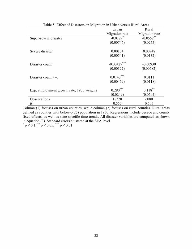
Table 5: Effect of Disasters on Migration in Urban versus Rural Areas Urban Rural Migration rate Migration rate Super-severe disaster -0.0129* -0.0552** (0.00746) (0.0255) Severe disaster 0.00104 0.00748 (0.00541) (0.0132) Disaster count -0.00427*** -0.00930 (0.00127) (0.00582) Disaster count >=1 0.0143*** 0.0111 (0.00469) (0.0118) Exp. employment growth rate, 1930 weights 0.290*** 0.118** (0.0249) (0.0504) Observations 18328 6080 R2 0.557 0.505

Column (1) focuses on urban counties, while column (2) focuses on rural counties. Rural areas defined as counties with below-p(25) population in 1930. Regressions include decade and county fixed effects, as well as state-specific time trends. All disaster variables are computed as shown in equation (3). Standard errors clustered at the SEA level. * p < 0.1, ** p < 0.05, *** p < 0.01

33

Table 6: Effect of Disasters on Migration - Good versus Bad Weather Areas (1) (2) (3) All Good weather Bad weatherSuper-severe disaster -0.0241** -0.0186 -0.0227* (0.0101) (0.0130) (0.0117) Severe disaster 0.00352 -0.00489 0.00757 (0.00621) (0.00925) (0.00652) Disaster count -0.00538*** -0.00924*** -0.00197 (0.00173) (0.00271) (0.00161) Disaster count >=1 0.0125** 0.0191** 0.00369 (0.00536) (0.00873) (0.00548) Exp. employment growth rate, 1930 weights 0.270*** 0.257*** 0.284*** (0.0246) (0.0311) (0.0380) Observations 20976 10488 10488 R2 0.512 0.485 0.522

Column (1) focuses on all counties that have weather information. Column (2) focuses on counties that experience good weather, while column (3) focuses on counties that experience bad weather. Good weather areas are defined as counties with above median score in their good weather index, computed as: winter average temperature in year 2000 divided by its standard deviation cross-county, minus summer average temperature in year 2000 divided by its standard deviation cross-county. Regressions include decade and county fixed effects, as well as state-specific time trends. The first three disaster variables are computed as shown in equation (3). Standard errors clustered at the SEA level. * p < 0.1, ** p < 0.05, *** p < 0.01

34

Table 7: Effect of Disasters on Migration by Race (1) (2) Migration rate

(black) Migration rate

(white) Super-severe disaster -0.0911 -0.0203* (0.195) (0.0117) Severe disaster -0.0948 -0.000794 (0.221) (0.00661) Disaster count 0.0524 -0.00450** (0.0665) (0.00193) Disaster count >=1 -0.323 0.0147** (0.258) (0.00662) Exp. employment growth rate, 1930 weights 1.132** 0.273*** (0.575) (0.0228) Observations 20567 21357 R2 0.179 0.472

In column (1) we study migration patterns for blacks and in column (2) we focus on whites. Regressions include decade and county fixed effects, as well as state-specific time trends. All disaster variables are computed as shown in equation (3). Migration by race is not available in 1980. Standard errors clustered at the SEA level. * p < 0.1, ** p < 0.05, *** p < 0.01

35

Table 8: Effect of Disasters on Migration by Disaster Type (1) Migration rate Flood count 0.00393* (0.00230) Storm count -0.00262** (0.00115) Tornado count 0.00153 (0.00330) Hurricane count -0.0129** (0.00566) Drought count 0.0184** (0.00784) Volcano count -0.0373** (0.0157) Earthquake count -0.00522 (0.0282) Other disasters (count) -0.0139*** (0.00467) Disaster count >=1 -0.00270 (0.00507) Exp. employment growth rate, 1930 weights 0.272*** (0.0227) Observations 24408 R2 0.525

We study the migration of the entire population. Regressions include decade and county fixed effects, as well as state-specific time trends. These disasters are not computed using equation (3). Standard errors clustered at the SEA level. * p < 0.1, ** p < 0.05, *** p < 0.01

36

Table 9: Effect of Disasters on Poverty Rate and House Values (1) (2) (3) House value

(log median) House rent

(log median) Poverty Rate

Super-severe disaster -0.0669*** -0.0370*** 0.0111*** (0.0154) (0.0109) (0.00321) Severe disaster -0.0148 -0.00136 0.00312 (0.0131) (0.00948) (0.00231) Disaster count 0.000182 0.000776 -0.00103** (0.00237) (0.00194) (0.000513) Disaster count >=1 0.00913 0.0111 -0.00236 (0.00936) (0.00780) (0.00191) Exp. employment growth rate, 0.243** 0.219** -0.148*** 1970 weights (0.109) (0.0936) (0.0214) Observations 15154 15152 15152 R2 0.977 0.974 0.870

In column (1) we study county-level decade mean of poverty rates. In columns (2) and (3) we focus on (log) house values and monthly rents at the end of each decade. Regressions include decade and county fixed effects. All disaster variables are computed as shown in equation (3). Regressions encompass the period 1960-2000. Standard errors are clustered at the SEA level. * p < 0.1, ** p < 0.05, *** p < 0.01

37

Figure 1: Annual disaster count by data source

This graph plots the summation of county-level disaster counts by year and source. Note that this measure will treat a given natural event that occurred in two separate counties as two different disaster events. Disaster count is truncated at 3000.

38

Figure 2: Disaster count by county, 1930-2010

This map plots disaster counts within each county for the whole period 1930-2010. Marker size is strictly increasing in number of events, while color represents quartiles [max=87].

39

Figure 3: Count of decades with a severe disaster event by county, 1930-2010

This map shows the number of decades with severe events per county in the period 1930-2010. Severe events are disasters associated to 10 or more deaths. Marker size is strictly increasing in number of events, while color represents quartiles [max=8].

40

Figure 4: Count of decades with a super-severe disaster event by county, 1930-2010

This map shows the number of decades with super-severe events per county in the period 1930-2010. Super-severe events are disasters associated to 100 or more deaths. Marker size is strictly increasing in number of events, while color represents quartiles [max=6].