understanding the effects of climate on airfield … · understanding the effects of climate on...
TRANSCRIPT

UNDERSTANDING THE EFFECTS OF CLIMATE ON AIRFIELD PAVEMENT DETERIORATION RATES
THESIS
Justin C. Meihaus, Captain, USAF
AFIT-ENV-13-M-16
DEPARTMENT OF THE AIR FORCE AIR UNIVERSITY
AIR FORCE INSTITUTE OF TECHNOLOGY
Wright-Patterson Air Force Base, Ohio
DISTRIBUTION STATEMENT A APPROVED FOR PUBLIC RELEASE; DISTRIBUTION IS UNLIMITED

The views expressed in this thesis are those of the author and do not reflect the official policy or position of the United States Air Force, Department of Defense, or the United States Government.

AFIT-ENV-13-M- 16
UNDERSTANDING THE EFFECTS OF CLIMATE ON AIRFIELD PAVEMENT DETERIORATION RATES
THESIS
Presented to the Faculty
Department of Systems and Engineering Management
Graduate School of Engineering and Management
Air Force Institute of Technology
Air University
Air Education and Training Command
In Partial Fulfillment of the Requirements for the
Degree of Master of Science in Engineering Management
Justin C. Meihaus, B.S.
Captain, USAF
March 2013
DISTRIBUTION STATEMENT A APPROVED FOR PUBLIC RELEASE; DISTRIBUTION IS UNLIMITED

AFIT-ENV-13-M-16
UNDERSTANDING THE EFFECTS OF CLIMATE ON AIRFIELD PAVEMENT
DETERIORATION RATES
Justin C. Meihaus, B.S. Captain, USAF
Approved:
___________________________________ __________ Alfred E. Thal, Jr., PhD (Chairman) Date ___________________________________ __________ George W. Van Steenburg (Member) Date ___________________________________ __________ M.Y. Shahin, PhD (Member) Date

AFIT-ENV-13-M-16
iv
Abstract
Over the past two decades, pavement engineers at the Air Force Civil Engineer
Center have noticed the majority of identified distresses from PCI airfield surveys are
climate related. To verify these trends, a comprehensive analysis of the current airfield
pavement distress database was accomplished based on a climate region perspective. A
four-zone regional climatic model was created for the United States using geospatial
interpolation techniques and climate data acquired from WeatherBank Inc. Once the
climatic regional model was developed, the climate information for each installation was
imported into the Air Force pavement distress database within PAVERTM. Utilizing the
pavement condition prediction modeling function in PAVERTM, pavement deterioration
models were created for every pavement family at each base in each climatic zone. This
was done to generate a list of bases that may have multiple pavement families with rates
of deterioration that are better or worse than the regional rates of deterioration. The
average regional rates of deterioration for each pavement family were found to be within
the parameters of conventional wisdom observed in Asphalt Concrete (AC) and Portland
Cement Concrete (PCC). The results of the pairwise comparisons using the Student’s T-
test determined the Freeze-Dry climate region deterioration rates for the PCC pavement
family were statistically different than the other three regions. No significant statistical
differences were observed in the AC pavement comparisons. This analysis established a
foundation to investigate and identify variables causing the rates of deterioration at
specific installations to differ from the regional rates of deterioration.

AFIT-ENV-13-M-16
v
I would like to dedicate this thesis to my wife and my daughter. Without their love, support, and encouragement I would not be where I am today. From the bottom of my
heart, thank you.

vi
Acknowledgments
I would like to express my deepest gratitude to my wife. You truly are my best
friend in the journey of marriage. I will never forget the early morning coffee runs and
the amazing breakfasts to jump-start my day. I am so thankful for your love and
dedication. I cannot say thank you enough for your unending support over the past 18
months. I would, also, like to thank my research advisor, for his advice, guidance and
support throughout this endeavor. You guided and challenged me every step of the way,
which ensured that I developed a solid foundation of knowledge and know how for
solving complex problems. For that I am truly grateful. This research effort would not
have been possible without the unending support and expertise of my thesis committee. I
am truly indebted to you both for your valuable insight and expertise that you provided
throughout this effort. I am truly grateful for the time you spent explaining the intricate
details of pavement management, pavement management and distresses, and PAVERTM.
Justin C. Meihaus

vii
Table of Contents
Page
Abstract .............................................................................................................................. iv
Acknowledgments .............................................................................................................. vi
List of Figures .................................................................................................................... ix
List of Tables ..................................................................................................................... xi
1.0 Introduction ..................................................................................................................1
1.1 Background ...............................................................................................................1 1.2 Problem Statement ....................................................................................................5 1.3 Research Objectives ..................................................................................................6 1.4 Methodology .............................................................................................................6 1.5 Overview ...................................................................................................................9
2.0 Literature Review .........................................................................................................10
2.1 Asset Management ..................................................................................................10 2.2 Pavement Management Systems .............................................................................14
2.2.1 Inventory Definition ....................................................................................... 18 2.2.2 Pavement Inspection ...................................................................................... 19
2.2.2.1 Structural Evaluations ............................................................................ 20 2.2.2.2 Friction Characteristic Evaluation .......................................................... 22
2.2.3 Condition Assessment .................................................................................... 23 2.2.4 Condition Prediction ...................................................................................... 25
2.4 Environmental Factors Affecting Pavement Deterioration .....................................29 2.4.1 Temperature ................................................................................................... 30 2.4.2 Precipitation and Subsurface Moisture .......................................................... 31 2.4.3 Freeze/thaw weakening .................................................................................. 32
2.5 Regional Climate Model .........................................................................................36 2.5.1 Environmental Factors for Climate Model ..................................................... 36 2.5.2 Quantitative Spatial Analysis ......................................................................... 38
2.6 Literature Review Summary ...................................................................................40
3.0 Methodology ................................................................................................................41
3.1 Developing Climate Zones ......................................................................................41 3.2 Developing Pavement Deterioration Rates .............................................................44 3.3 Statistical Analysis ..................................................................................................45 3.4 Methodology Summary ...........................................................................................49

viii
Page
4.0 Results and Analysis ....................................................................................................50
4.1 Regional Climate Zone Model ................................................................................50 4.2 Rates of Deterioration .............................................................................................53 4.3. Statistical Analysis ................................................................................................54
4.3.1 No Freeze-Wet Climate Region ..................................................................... 55 4.3.2 No Freeze-Dry Climate Region ...................................................................... 58 4.3.3 Freeze-Wet Climate Region ........................................................................... 61 4.3.4 Freeze-Dry Climate Region ........................................................................... 65 4.3.5 Overall Observations ...................................................................................... 68 4.3.6 ANOVA Results ............................................................................................. 70
5.0 Conclusions and Recommendations ............................................................................77
5.1 Conclusions of Research .........................................................................................77 5.2 Limitations ..............................................................................................................80 5.3 Future Research .......................................................................................................82
Appendix A - JMP Models ................................................................................................84
Appendix B - Rates of Deterioration Tables ......................................................................92
References ..........................................................................................................................96
ix
List of Figures
Page Figure 1. Factors Affecting Pavement Performance ........................................................... 4
Figure 2. Family Definition Tree ........................................................................................ 7
Figure 3. Conceptual Illustration of a Pavement Condition Life-cycle ............................ 15
Figure 4. Pavement Condition Index (PCI) Rating Scale ................................................. 24
Figure 5. Pavement Section Prediction in Relation to the Family Model ........................ 29
Figure 6. WeatherBank U.S. Weather Station Locations ................................................. 42
Figure 7. Distribution Areas ............................................................................................. 47
Figure 8. Kriging Maps for Precipitation and Freezing Degree-Days .............................. 51
Figure 9. Climate Zone Map for the United States ........................................................... 52
Figure 10. PAVERTM Prediction Modeling Output .......................................................... 53
Figure 11. Freeze-Wet Taxiway-Concrete Distribution ................................................... 62
Figure 12. No Freeze-Wet Runway-PCC Distribution ..................................................... 84
Figure 13. No Freeze-Wet Runway-AC/AAC Distribution ............................................. 84
Figure 14. No Freeze-Wet Taxiway-PCC Distribution .................................................... 84
Figure 15. No Freeze-Wet Taxiway-AC/AAC Distribution ............................................. 85
Figure 16. No Freeze-Wet Apron-PCC Distribution ........................................................ 85
Figure 17. No Freeze-Wet Apron-AC/AAC Distribution ................................................. 85
Figure 18. No Freeze-Dry Runway PCC Distribution ...................................................... 86
Figure 19. No Freeze-Dry Runway AC/AAC Distribution .............................................. 86
Figure 20. No Freeze-Dry Taxiway PCC Distribution ..................................................... 86
Figure 21. No Freeze-Dry Taxiway AC/AAC Distribution .............................................. 87

x
Page
Figure 22. No Freeze-Dry Apron PCC Distribution ......................................................... 87
Figure 23. No Freeze-Dry Apron AC/AAC Distribution ................................................. 87
Figure 24. Freeze-Wet Runway PCC ................................................................................ 88
Figure 25. Freeze-Wet Runway AC/AAC ........................................................................ 88
Figure 26. Freeze-Wet Taxiway PCC (with Outliers) ...................................................... 88
Figure 27. Freeze-Wet Taxiway PCC (with outliers removed) ........................................ 89
Figure 28. Freeze-Wet Taxiway AC/AAC (with outliers) ................................................ 89
Figure 29. Freeze-Wet Taxiway AC/AAC (with outliers removed) ................................. 89
Figure 30. Freeze-Wet Apron PCC (with outliers) ........................................................... 90
Figure 31. Freeze-Wet Apron PCC (with outliers removed) ............................................ 90
Figure 32. Freeze-Dry Runway PCC ................................................................................ 90
Figure 33. Freeze-Dry Runway AC/AAC ........................................................................ 91
Figure 34. Freeze-Dry Taxiway PCC ............................................................................... 91
Figure 35. Freeze-Dry Taxiway AC/AAC ........................................................................ 91
Figure 36. Freeze-Dry Apron PCC ................................................................................... 92
Figure 37. Freeze-Dry Apron AC/AAC ............................................................................ 92

xi
List of Tables
Page
Table 1. Moisture Related Distresses in Flexible (AC) .................................................... 34
Table 2. Moisture Related Distress in rigid (PCC) pavements ......................................... 35
Table 3. Distribution of Air Force Bases for each Climate Zone ..................................... 51
Table 4. No Freeze-Wet Rate of Deterioration Summary Table ...................................... 56
Table 5. No Freeze-Wet List of Bases Above 1 Standard Deviation ............................... 57
Table 6. No Freeze-Wet List of Bases Below 1 Standard Deviation ................................ 57
Table 7. No Freeze-Dry Rate of Deterioration Summary Table ....................................... 59
Table 8. No Freeze-Dry List of Bases above 1 Standard Deviation ................................. 59
Table 9. No Freeze-Dry List of Bases below 1 Standard Deviation ................................. 59
Table 10. Freeze-Wet Rate of Deterioration Summary Table .......................................... 63
Table 11. Freeze-Wet List of Bases Above 1 Standard Deviation ................................... 65
Table 12. Freeze-Wet List of Bases Below 1 Standard Deviation ................................... 65
Table 13. Freeze-Dry Rate of Deterioration Summary Table ........................................... 66
Table 14. Freeze-Dry List of Bases Above 1 Standard Deviation ................................... 67
Table 15. Freeze-Dry List of Bases Below 1 Standard Deviation .................................... 67
Table 16. Overall Climate Zone Average Rates of Deterioration-PCC ............................ 68
Table 17. Overall Climate Zone Average Rates of Deterioration-AC .............................. 69
Table 18. Student's T-Test Comparison for PCC Runways .............................................. 71
Table 19. Student's T-Test Comparison for PCC Taxiways ............................................. 72
Table 20. Student's T-Test Comparison for PCC Aprons ................................................. 72
Table 21. Student's T-Test Comparison for AC Runways ............................................... 75

xii
Page
Table 22. Student's T-Test Comparison for AC Taxiways ............................................... 75
Table 23. Student's T-Test Comparison for AC Aprons ................................................... 76
Table 24. No Freeze-Wet Rates of Deterioration Data ..................................................... 93
Table 25. No Freeze-Dry Rates of Deterioration Data ..................................................... 94
Table 26. Freeze-Wet Rates of Deterioration Data ........................................................... 94
Table 27. Freeze-Dry Rates of Deterioration Data ........................................................... 95

1
UNDERSTANDING THE EFFECTS ON CLIMATE ON AIRFIELD PAVEMENT
DETERIORATION RATES
1.0 Introduction
1.1 Background
The United States government, Department of Defense (DoD), and Air Force are
facing a pivotal point in their history due to massive reductions to the overall government
budget. The DoD is on the cusp of a reduction of $478 billion dollars over 10 years. The
Air Force is not exempt from these cuts and will have to overcome a reduction of
approximately $12 billion in their operating budget over the next 10 years while still
maintaining the ability to execute its mission. Large portions of the cuts will affect the
maintenance and repair budgets used to maintain the Air Force’s aging infrastructure. As
a result, Air Force engineers are exploring and developing new innovative processes and
procedures for accomplishing a strategic approach to managing facility and infrastructure
assets.
Asset management, often referred to as Facility Management (FM), consists of
tools developed over the past 20 years in the public and private sectors to effectively
manage facility and infrastructure assets. The International Infrastructure Management
Manual (IIMM) describes asset management as “the combination of management,
financial, economic, engineering and other practices applied to physical assets with the
objective of providing the required level of services in the most cost effective manner”
(American Association of State Highway and Transportation Officials, 2011). FM
embraces these concepts in an attempt to provide and maintain adequate facilities and

2
infrastructure to the built environment, which could be a large city or military
installation. However, accomplishing FM is a monumental challenge when dealing with
unrelenting budgets cuts and massive reductions in workforces (Cotts, Roper, & Payant,
2010). To address this challenge within the Air Force, new principles and practices must
be identified and created to facilitate a new era of asset and infrastructure management.
The Civil Engineer (CE) community has responded and is in the process of implementing
asset management as the foundation of CE operations in “Building Sustainable
Installations,” which is one of three goals identified in the 2011 U.S. Air Force Civil
Engineer Strategic Plan. One aspect of this plan involves the maintenance and
management of airfield pavements to enable the safe and efficient movement of air and
space craft. Critical to this effort is the use of pavement deterioration models as a
management tool to enable installation engineers to meet the required level of service in
the most cost effective manner.
Pavement deterioration models can enhance the capabilities of a pavement
management system, thereby producing an effective tool for pavement engineers. These
models allow pavement engineers to predict the timing for maintenance and rehabilitation
activities and to estimate the long-range funding requirements for preserving the airfield
pavement system (Sadek, Freeman, & Demetsky, 1996). Performance prediction models
are crucial to the management of pavements at both the network and project levels. At
the network level, these models are used for the selection of optimal Maintenance &
Rehabilitation (M&R) strategies, condition forecasting, budget planning, scheduling
inspections, and working planning (Shahin, 2005). Prediction models are used at the
project level to assist with design and life-cycle costs analyses (Gendreau & Soriano,

3
1998). Network level prediction models can also be used to identify and select
rehabilitation alternatives to meet expected traffic and climate conditions (Shahin, 2005).
Deterioration models predict the deterioration rate of a pavement section over
time to enable managers to predict M&R activities well into the future. In contrast,
functional performance models predict the present serviceability index, often called the
Pavement Condition Index (PCI). Starting in 1968, the U.S. Army Construction
Engineering Research Laboratory (USACERL) began developing an objective and
repeatable rating system to be used to provide an index of a pavement’s structural
integrity and surface operational condition (Shahin, 2005). Their research led to the
development of the PCI. PCI is a numerical index that measures pavement condition on a
scale from 0 to 100, with 0 being a failed pavement section and 100 being a
perfect/newly installed pavement section (Shahin, 2005). The PCI is based on the results
of a visual condition survey in which distress type, severity, and quantity are identified
(Shahin, 2005). PCI condition surveys provide pavement engineers insight into whether
load-related factors or climate-related factors led to the cause of distresses (Shahin,
2005). The PCI is the distress condition rating system that the Air Force currently uses
for pavement management activities. The surface distress data used to calculate PCIs, for
Air Force airfields, are collected through the extensive airfield evaluation program
managed by pavement engineers located at the Air Force Civil Engineer Center-East.
Airfield pavements must be able to function all over the world in a wide array of
environmental conditions supporting multiple types of aircraft. Haas (2001) identifies
five key factors affecting pavement performance, as shown in Figure 1. Each one of
these identified factors can affect pavement performance with varying degrees of

4
magnitude. Environmental, or climate, conditions can have significant impacts on the
pavement and sub-grade materials, which can radically affect the performance lifespan of
a pavement. Notable environmental factors that affect pavement performance are
temperature, precipitation, subsurface-moisture, and freeze-thaw cycles (Li, Mills, &
McNeil, 2011). Typically, pavements are designed to minimize extreme damage due to
temperature. For example, eliminating frost susceptible materials frost heave effects can
be minimized. Using properly designed asphalt binders that perform well in cold
temperatures can minimize thermal cracking in flexible pavements. However pavements
will deteriorate over time due to environmental factors even with the correct design. In
essence, environmental factors can affect both the structural and functional capacities of
airfield pavements.
Figure 1. Factors Affecting Pavement Performance (Haas, 2001)

5
The current Air Force predictive models are developed using PAVERTM, a
pavement management software program. PAVERTM uses surface distress data collected
from an airfield survey to calculate PCI values for each type of pavement family. Shahin
(2005) defines a pavement family as a group of pavement sections with similar
deterioration characteristics. In turn, the PCI values are used to create a performance
predictive model for a specific pavement family. Developing a regional climatic
pavement deterioration model would allow pavement engineers to identify bases with
rates of deterioration that are greater than or less than the regional model. This will help
pavement engineers identify and investigate factors affecting the rate of deterioration.
Future research could then be conducted to identify an individual base’s M&R and design
strategies that are could be contributing to the degradation of the pavement performance
or are extending the lifespan of the pavement network.
1.2 Problem Statement
The Air Force has over 1.6 billion square feet of concrete and asphalt pavements
in its current infrastructure inventory. Over the past two decades, pavement engineers at
AFCEC-East have noticed the majority of the identified distresses from the PCI airfield
surveys are climate related. To verify these trends, a comprehensive analysis of the
current airfield pavement distress database must be accomplished based on a climate
region perspective. There are a number of climatic models that exist however; the
models data were outdated and not suitable for the analysis of pavement deterioration.
Therefore, a regional climatic model must be created to conduct this type of analysis.
Generating a regional climate model will allow an in-depth analysis of how the average

6
rates of deterioration of bases compare to that of a climatic regional rate of deterioration.
Furthermore, this analysis will establish a baseline that will allow pavement engineers to
investigate and identify, through future research, which variables are causing average
rates of deterioration to differ from the regional rates of deterioration.
1.3 Research Objectives
The objective of this research was to answer the question: How can climate
regions, within the United States, be used to understand and quantify the effects of
climatic conditions on the deterioration rates of airfield pavements? To effectively
answer this question, the following investigative questions were addressed.
1. What climatic/environmental variables should be used to develop a regional climate model for pavement deterioration modeling?
2. How do the regional climate-based average rates of deterioration for each family of pavements compare to the individual base average rates of deterioration for each family of pavements within the same region?
3. Are the climate based regional average rates of deterioration statistically different from one another?
These research objectives revolve around establishing an understanding of how
environmental factors affect pavement deterioration rates and developing a conceptual
process to evaluate the effects of environmental factors on pavement deterioration rates.
1.4 Methodology
The methodology used to accomplish the main goal of this research effort had
three major parts. The first part created four regional climate zones for the continental
United States, Hawaii, and Alaska and classifies each Air Force base with an operational

7
airfield into one of the four zones. The second part used the climate zones and the PCI
survey data to create a regional pavement deterioration models for each base and for each
family of pavements defined in Figure 2. The third phase was to conduct a statistical
examination of the individual, regional, and overall average rate of deterioration for each
of the family of pavements.
Figure 2. Family Definition Tree (Shahin, 2005)
Initial efforts to find a suitable climate model for the research were not successful.
The Federal Highway Administration (FHWA) was contacted to acquire information
regarding their climate zone model, but was informed that the model was developed in
the early 1990s and was out of date and had not been updated. Therefore, research was
conducted to find environment/climate variables that effect pavement deterioration within
the relevant literature. Four variables, temperature, precipitation, subsurface moisture,
and freeze-thaw cycles, were identified as having the most significant impact on
pavement deterioration. Precipitation and Freezing-Degree-Day (FDD) data was

8
acquired from WeatherBank Inc. located in Edmond, Oklahoma, to build the climate
model for this research effort. WeatherBank continuously collects data from
approximately 1,700 National Oceanic and Atmospheric Administration (NOAA),
National Weather Service (NWS), and Federal Aviation Administration (FAA) stations
scattered across the United States, including Alaska and Hawaii. The data provided was
collected from 1982 through 2011. A 30-year average value for precipitation and FDD
was provided for each of the 1,700 stations. To create a climate model, ArcGIS’s
geostatistical interpolation capabilities and the WeatherBank data was used to create four
climate zones: Freeze-Dry, Freeze-Wet, No Freeze-Dry, and No Freeze-Wet. The
specific thresholds that defined each of the zones were established through the guidance
of engineers at the U.S. Army Cold Regions Research and Engineering Laboratory.
Once the climatic regional models were developed, the climate information was
imported into the Air Force pavement distress database within PAVERTM. To generate
regional pavement deterioration models, the PAVERTM database was first organized into
pavement family types, i.e., Portland Cement Concrete (PCC), Asphalt Concrete (AC),
and composite pavements (AC/PCC combination), and then by pavement usage
categories, i.e., runways, taxiways, and aprons. Figure 2 is an example of a family
definition tree using the pavement factors: use, type, and rank. This figure is a
representation of how the data was organized to enable PAVERTM to develop the
pavement deterioration models.
Utilizing the pavement condition prediction modeling function in PAVERTM,
pavement deterioration models were created for every pavement family at each base in
each climatic zone. The final phase of this study was a statistical examination of the
9
individual, regional, and overall average rate of deterioration for each family of
pavements. This will assist with identifying bases that have average rates of deterioration
above and below 1 standard deviation from the regional rate of deterioration. The final
part of the statistical analysis was to conduct an analysis of variance (ANOVA) to test the
hypothesis that the climate region rates of deterioration for each family of pavements are
statistically different from one another and different from the Air Force overall rate of
deterioration for each pavement family.
1.5 Overview
This chapter established the background and objectives for this research effort.
Chapter 2 examines existing literature relating to pavement management systems,
pavement conditions surveys, pavement deterioration, and pavement condition prediction
models. Chapter 3 discusses the methodology used for the three phases of developing the
new climatic pavement prediction deterioration models. Chapter 4 discusses the results
from generating a climate model with four zones and the statistical analysis of the
regional average rates of deterioration. Finally, Chapter 5 provides a discussion of the
findings and conclusions of the research effort along with recommendations for future
research on this topic.

10
2.0 Literature Review
This chapter discusses the current practices and body of knowledge for pavement
management principles, techniques, and systems. It also discusses how pavement
management systems utilize predictive performance models to enhance a decision-
maker’s capabilities of creating and implementing maintenance and rehabilitation
strategies. Furthermore, this chapter discusses the effects of certain environmental
factors on pavement deterioration and performance.
2.1 Asset Management
The United States government, Department of Defense (DoD), and Air Force are
facing fiscal uncertainty for the foreseeable future. The political volatility in
Washington, D.C., is triggering a wave of budget cuts and constraints across the entire
federal government. In 2013, the DoD will operate with a reduced budget and the threat
of looming sequestration cuts. The FY 2013 budget has reduced defense spending $5.2
billion from 2012 and will reduce planned spending by $487 billion over the next 10
years (Chief Financial Officer, 2012). The American Taxpayer Relief Act of 2012
deferred proposed sequestration budget cuts, from the Budget Control Act, until March 1,
2013. The proposed sequestration will cut the DoD by $500 billion, on top of the $478
billion in cuts already proposed over the next 10 years (Garamone, 2012). DoD officials
have warned top political officials that these sequestration cuts will “blow the bottom out
of the defense strategic guidance released in early 2012” (Garamone, 2012). Efforts are
currently underway, on all fronts, to reduce federal spending across the full spectrum of

11
the federal government in an attempt to reduce the federal deficit, which in turn has
significant impacts on the DoD and the Air Force. Memorandums released by the
Deputy Secretary of Defense and the Under Secretary of the Air Force in early 2013
paved the path to “implement immediate prudent actions to mitigate probable budget
reductions” (Carter, 2013).
Large portions of the cuts will affect the maintenance and repair budgets used to
maintain the Air Force’s aging infrastructure, including airfield pavements. Aging
infrastructure, both on and off of military installations, are deteriorating at a rapid rate
due to the lack of adequate funds designated for maintenance and repair in most annual
operating budgets. The Air Force is not exempt from the challenges of managing old and
outdated infrastructure while striving to maintain the ability to support the mission
directives of the DoD. In 2011, Gen. Norton Schwartz, Air Force Chief of Staff, stated
the Air Force “will play a role in the solution not by retrenching or continuing business as
usual on a reduced scale…” but by making “difficult choices to balance near-term
operational readiness with longer term needs and fit all of that into a more affordable
package” (Air Force Civil Engineer, 2011, p. 2). As a result, Air Force engineers are
exploring and developing new innovative processes and procedures for accomplishing a
strategic approach to managing facility and infrastructure assets.
The Air Force Civil Engineer mission is to “provide, operate, maintain, and
protect sustainable installations as weapon-systems platforms through engineering and
emergency response services across the full mission spectrum” (Air Force Civil Engineer,
2011). To accomplish this mission, the Civil Engineer (CE) community has developed
the following three main strategic goals to meet the challenges facing the Air Force in

12
near future: Build ready engineers, Build great leaders, and Build sustainable
installations. To address these challenges within the Air Force, new principles and
practices must be identified and created to facilitate a new era of asset and infrastructure
management. The CE community has responded and is in the process of implementing
asset management as the foundation of CE operations in “Building Sustainable
Installations,” which is the third goal identified in the 2011 U.S. Air Force Civil Engineer
Strategic Plan.
Asset management, often referred to as facility management (FM), consists of
tools developed over the past 20 years in the public and private sectors to effectively
manage facility and infrastructure assets. The International Infrastructure Management
Manual describes asset management as “the combination of management, financial,
economic, engineering and other practices applied to physical assets with the objective of
providing the required level of services in the most cost effective manner” (AASHTO,
2011, p. 1-11). FM embraces these concepts in an attempt to provide and maintain
adequate facilities and infrastructure in the built environment, which could be a large
city’s roadway network or military installation’s airfield network. However,
accomplishing FM is a monumental challenge when dealing with unrelenting budgets
cuts and massive reductions in workforces (Cotts, Roper, & Payant, 2010). Airfield
pavements represent a major asset in the Air Force’s infrastructure inventory.
Preservation of this asset is of the upmost importance, which requires solid design and
construction techniques and standards, quality management practices, robust inspection
programs, innovative technology, and adequate financing.

13
In the public sector, Transportation Asset Management (TAM) is a branch of
Asset Management that has gained strength over the past decade. The American Public
Works Association Asset Management Task Force defines TAM as “…a methodology
needed by those who are responsible for efficiently allocating generally insufficient funds
amongst valid and competing needs” (Office of Asset Management, 1999). This quote
sheds light on the new fiscal environment that Civil Engineers face for the foreseeable
future due to the current fiscal situation in the federal government. Asset Management
and Transportation Asset Management are holistic concepts that help managers and
decision-makers organize, plan, and implement goals and objectives. Asset managers
most accomplish these tasks while maintaining their responsibility to optimize
expenditures and to maximize the value of the assets over its life-cycle. The International
Infrastructure Management Manual (IIMM) describes the purpose of TAM as “to meet a
required level of service, in the most cost effective manner, through the management of
assets for present and future conditions” (AASHTO, 2011, p. 1-12). In essence, the main
goal of TAM is to build, maintain, and operate facilities in the most cost-effective manner
while providing the best value to the stakeholder or customer. TAM can touch nearly
every aspect of a transportation agency’s business, to include everything from planning,
engineering, construction, and maintenance. TAM or AM is a way of doing business that
brings a particular perspective to how a public agency or federal entity should conduct
daily business.
The benefits of implementing a comprehensive asset management plan can be
seen in a variety of ways. Asset management plans provide a long-term view for
organizations. This puts an emphasis on managing assets throughout the duration of their

14
life-cycle, which could be 40 years or longer (AASHTO, 2011). This provides a level of
comfort to the stakeholders by knowing that the assets are being managed for their
expected lifespan. A properly executed TAM plan will have its principles and practices
integrated into every level of the organization. A strategic TAM plan will deliver the
desired level of service to the customer or stakeholder, through sound financial planning
coupled with solid management plans and concise reporting tools (AASHTO, 2011).
Furthermore, transportation assets such as airfields are costly to build, maintain, operate
and use. Therefore, stressing the importance of life-cycle analysis, the AASHTO
Transportation Asset Management Guide states, “TAM helps to ensure that the benefits
delivered by the network are maximized while the cost of providing, maintaining, and
using it are minimized” (AASHTO, 2011, p. 1-13). A well designed asset management
plan and process can provide an organization a comprehensive picture of asset
performance. Air Force engineers use a variety of asset management tools to develop a
comprehensive picture of the wide range of facility and infrastructure assets that exist on
an installation. In the pavement arena, engineers use the pavement management systems
approach to accomplish the strategic goals of asset management.
2.2 Pavement Management Systems
Airfield managers and engineers go to great lengths to ensure that the pavement
associated with an airfield are safe for flying operations every day of the year. In the Air
Force, this enormous responsibility is accomplished through teams of expert engineers at
the Air Force Civil Engineer Center (AFCEC), at the respective Air Force Major
Commands (MAJCOM), and local engineers at the respective installations. To

15
effectively manage the 1.6 billion square feet of concrete and asphalt pavements, Air
Force engineers have implemented a Pavement Management (PM) system. A PM system
is a systematic tool that enables effective and economical management of an entire
pavement network. Shahin (2005, p. 1) describes a PM system as “a systematic,
consistent method for selecting Maintenance and Rehabilitation (M&R) needs and
determining priorities and the optimal time of repair by predicting future pavement
condition.” PM systems are designed to assist decision-makers in finding strategies for
funding and maintaining pavements to a specified condition over time in the most
economically feasible plan. According to Shahin and Walther (1990), 80% of the repair
costs can be avoided if M&R is performed before the rate of deterioration of the
pavement increases sharply, as shown in Figure 3. Neglecting the importance of routine
pavement inspections to identify distresses that are in need of repair in a pavement
network has negative financial consequences.
Figure 3. Conceptual Illustration of a Pavement Condition Life-cycle (Shahin, 2005)

16
As the backbone of the installation weapon-system, airfields require constant
investment and attention to maintain an adequate pavement network for flying operations.
The Air Force does have installations that have pavements that were originally
constructed in the 1940s and 1950s that still exist. The fact that these pavements are still
serviceable is due to the active maintenance programs on these installations, which
allows for a high operations tempo. However, the current fiscal climate does not warrant
the ability to replace full runways and/or aprons. Therefore, the maintenance program
must be proactive to extend the service life of existing pavements. Managing aging
pavement networks is a rather difficult task due to the complexity of pavement behavior
in the variety of climate regions across the United States. Through multiple years of
research, PM systems have been created and developed to provide a structured and
inclusive approach to pavement management.
A PM system can incorporate a variety of processes and tools to accomplish the
strategic goals of the pavement management organization. Pavement management is
conducted at two levels: at the network level and project level. Network-level
management is used for budgeting, planning, scheduling, and selecting of potential M&R
projects for an entire pavement network, such as an Air Force installation (Shahin &
Walther, 1990). To accurately select potential projects at this level, the future condition
of each section must be accurately predicted. Projecting the future condition of the
section enables two tasks to be performed. The first task is to schedule future inspections
for sections that have been flagged for having a high rate of deterioration. The second
task is to identify sections of pavement that will require major M&R in future years for
budget estimating (Shahin & Walther, 1990). Typically, these sections are flagged for

17
major M&R projects because their condition has reached a predetermined level. As seen
in Figure 3, this is the point at which the curve begins the sharp decline in condition and
major M&R projects should be executed. Therefore, network-level management requires
managers to consider the organization’s current and future budget needs, consider the
current and future network pavement condition, and identify and prioritize a list of
projects to be considered at the project level (Shahin & Walther, 1990). At the project
level, projects identified from the network-level analysis undergo an in-depth evaluation
to develop alternatives based on specific site conditions (Shahin & Walther, 1990). The
analysis done at this level will produce a list with the most cost-effective M&R projects
within existing management or organization constraints (Shahin & Walther, 1990).
Pavement management engineers need a systematic approach to pavement management
to deliver the most strategic plans that deliver the best return on investment (Shahin,
2005).
The PM approach consists of six main steps: Inventory Definition, Pavement
Inspection, Condition Assessment, Condition Prediction, Condition Analysis, and Work
Planning. The first four steps will be discussed in detail over the next sections in this
chapter. This approach has evolved over 30 years of research and development of the
PAVERTM pavement management system (Shahin, 2005). Air Force, Army and Navy
pavement managers use this computer software pavement to automate the analysis and
storage of the data associated with a PM system. PAVERTM was initially developed in
the late 1970s to help the Department of Defense manage maintenance and repair
activities for its enormous pavement inventory (Colorado State University, 2012). The
development of this program was orchestrated under the backing of the U.S. Army Corps

18
of Engineers with funding from both the Air Force and the Army (Shahin & Walther,
1990). The program continues to be updated by the U.S. Army Corp of Engineers with
funding provided by the Air Force, Army, Navy, Federal Aviation Administration, and
the Federal Highway Administration. There are numerous other software programs
similar to PAVERTM; however, this program is used exclusively by the whole DoD to
analyze and summarize data collected from airfield inspections.
2.2.1 Inventory Definition
Inventory Definition breaks the pavement inventory into networks, branches, and
sections. A network is a logical grouping of pavements for M&R management. For
example, a military installation could have two networks, one for the base roadways and
one for all of the airfield pavements. Shahin (2005, p.2) defines a branch as “an easily
identifiable entity with one use, for example a runway, a taxiway, or a parking apron.” A
branch can be further subdivided into sections based on construction condition of
pavement and/or traffic. A section is the smallest pavement area and must consist of the
same pavement type, i.e., concrete or asphalt. A section is also the smallest management
unit in the PAVERTM PM systems, where M&R treatments are selected and applied.
Pavement managers must take into account factors such as pavement structure,
construction history, traffic, and pavement rank when determining how to break branches
into sections (Shahin, 2005). The next phase in the process is to conduct a pavement
inspection.

19
2.2.2 Pavement Inspection
Airfield inspections conducted on Air Force installations provide full spectrum
structural, surface distress, and friction airfield evaluations. This program provides
critical data to Air Force engineers to efficiently manage and effectively control airfield
pavements. According to AFI 32-1041, Airfield Evaluation Program, engineers use the
pavement strength, condition, and performance data to accomplish the following
(Department of the Air Force, 1994).
• Determine the size, type, gear configuration, and weight of aircraft that can safely operate from an airfield without damaging the pavement or the aircraft.
• Develop operations usage patterns for a particular aircraft pavement system (for example, parking, apron use patterns, and taxiway routing).
• Project or identify major maintenance or repair requirements for an airfield pavement system to support present or proposed aircraft missions. Evaluations provide engineering data to help in designing projects.
• Help airbase mission and contingency planning functions by developing airfield layout and physical property data.
• Develop and confirm design criteria.
• Help justify major pavement projects.
• Ensure flying safety by providing pavement surface data which quantify traction and roughness characteristics.
Initially, all pavement evaluation testing was destructive in nature, which caused
significant airfield closures and severely impacted airfield operations (Davit, Brown, &
Green, 2002). These tests were labor intensive and took as long as 8 hours to complete,
including time for repairs. Plate bearing tests were performed on rigid pavements and
California Bearing Ratio tests were performed on flexible pavements (Davit, Brown, &

20
Green, 2002). In the 1970s, non-destructive testing methods were introduced to reduce
the conflicts caused by closing the airfields for extended periods of time. Between 1985
and 1990, multiple new technologies were incorporated to minimize disruptions to
airfield operations, enhance ability to respond to contingencies, and reduce analysis and
reporting times (Davit, Brown, & Green, 2002).
There are three main types of evaluations that are performed during the
course of a pavement evaluation: airfield pavement structural evaluation, runway friction
characteristics, and airfield pavement condition index (PCI) surveys. Active airfields are
structurally evaluated on an 8-10 year cycle along with PCI surveys conducted every 3 or
5 years. The data collected from the surveys help base and command personal determine
the operational condition of pavements, prioritize repair and construction projects, and
determine whether an airfield structural pavement evaluation is needed (Department of
the Air Force, 1994). PCI surveys will be discussed in the Pavement Condition section of
this chapter.
2.2.2.1 Structural Evaluations
Airfield pavement structural evaluations determine a pavement‘s load-carrying
capacity by testing the physical properties of the pavement in its current condition
(Department of the Air Force, 1994). Typical equipment includes Heavy Weight Deflect
(HWD) meters, automated and manual dynamic cone penetrometers (DCPs), and
pavement core drills. The HWD test is one of the most widely used tests when assessing
the structural integrity of airfield pavements (Gopalakrishnan, 2008). This test is
conducted by dropping a large mass onto a circular metal plate, on which seven

21
deflection measurement sensors are attached to record the resultant forces and deflections
(Davit, Brown, & Green, 2002). This piece of equipment has the ability to impart a load
to the pavement with weights ranging from 6,500 pounds to 54,000 pounds (Davit,
Brown, & Green, 2002). The system uses an on-board computer to record the deflection
data and provides the operator with instantaneous deflection information that is stored for
further analysis (Davit, Brown, & Green, 2002). The ultimate goal of the HWD is to
replicate the force history and deflection magnitudes of a moving aircraft tire
(Gopalakrishnan, 2008).
The second tool often used for structural evaluation is the Dynamic Cone
Penetrometer (DCP) and the Automated DCP (ADCP). Results from the test can be used
to determine the soil type and California Bearing Ratio (CBR); it can also be used to
interpret soil layer thickness in underlying pavement layers (Davit, Brown, & Green,
2002). These tests consist of dropping a hammer with a known weight and drop height,
manually or mechanically, against an anvil that drives a cone into the soil. The number
of hammer blows is quantified in terms of a DCP index, which is a ratio of the depth of
penetration to the number of blows of the hammer (Davit, Brown, & Green, 2002). The
DCP index is then correlated to CBR.
The final structural evaluation that is conducted is core drills of rigid and flexible
pavements. The core drill is used to take pavement samples and gain access to the base,
subbabse, and subgrade so DCP and ADCP testing can be conducted and take soil
samples to characterize the soil type, layer thickness and calculate in-situ soil strength.
The cores are extracted from asphalt concrete and PCC pavements by a six-inch diameter
diamond-tipped coring barrel (Davit, Brown, & Green, 2002). At least one core sample

22
from each airfield feature is taken by HQ AFCEC Airfield Pavement Evaluation tea for
laboratory testing. These structural tests are used to get adequate data about the existing
airfield pavements to ensure that airfields are fully capable of supporting the flying
mission.
2.2.2.2 Friction Characteristic Evaluation
The second type of pavement evaluation conducted on Air Force airfields is a
friction characteristics evaluation. According to Air Force Instruction 32-1041, runway
friction characteristics evaluations assess a runway’s tractive qualities and hydroplaning
potential since they contribute to aircraft braking response. This evaluation has three
primary objectives: determine certain runway surface characteristics (such as slope and
texture), conduct measurements of the runway surface coefficient of friction, and assess
the capability of the runway to drain excess water and recover its friction properties
(AFCESA, 1994). Pavement surface transverse and longitudinal slopes are measured
every 500 feet along the entire length of the runway. Transverse slopes are measured at
distances of 5 and 15 feet on both sides of the runway centerline. The surface texture
measurement is conducted by a flow meter. The final test is completed through the use
of continuous friction measuring equipment. This equipment uses internal systems to
simulate rain-wetted pavement surface conditions during which friction measurements
are taken while the system is traveling at speeds between 40 and 60 miles per hour. This
test helps identify areas of the runway pavement that are smooth due to poor macro or
microtexture, excessive wear due to heavy traffic, aggregate polishing, heavy rubber
build-up, and/or oil/fuel spills (AFCESA, 1994).
23
2.2.3 Condition Assessment
One of the most important features of a solid PM system is the ability to
determine the current condition of a pavement network in order to predict a future
condition (Shahin, 2005). Starting in 1968, the U.S. Army Construction Engineering
Research Laboratory (USACERL) began developing an objective and repeatable rating
system to be used to provide an index of a pavement’s structural integrity and surface
operational condition (Shahin, 2005). Their research led to the development of the
Pavement Condition Index (PCI).
The PCI is a numerical index that measures pavement condition on a scale from 0
to 100, with 0 being the worst and 100 being perfect (Shahin, 2005). The PCI rating
system provides commanders a visual trigger regarding the level of maintenance and/or
repair activities that should be performed (Davit, Brown, & Green, 2002). Figure 4, is an
example of a PCI rating scale.

24
Figure 4. Pavement Condition Index (PCI) Rating Scale (Colorado State University,
2012)
The PCI is calculated based on the results of a visual survey in which distress
type, severity, and quantity are identified for a predetermined number of sample units.
(Shahin, 2005). The PCI survey is conducted by trained individuals to identify and
document pavement distresses caused by aircraft loading and environmental conditions.
The distresses used to calculate the PCI for both roadways and airfield pavements can be
found in the American Society for Testing and Materials D6433-11 and D5340-11,
respectively. The distress information collected during a pavement condition inspection
provides pavement managers insight into whether the distress is caused by repetitive
loading or overloading, climactic factors, or other factors such as construction-related
issues (Shahin, 2005). Shahin (2005, p. 17) states, “The degree of pavement deterioration
is a function of distress type, distress severity, and distress density.” However,
25
developing an index that accounted for all factors proved to be extremely difficult.
Therefore, “deduct values” are used as weighting factor’s to accurately account for the
effect that each combination of distress type, severity level, and distress density has on
pavement condition (Shahin, 2005). The PCI can either be calculated by hand or the
inspection data can be entered PAVERTM to help automate the calculations and analysis.
2.2.4 Condition Prediction
Predicting future pavement performance is a critical tool for pavement managers
and engineers. Pavement prediction modeling is an absolutely essential element of any
complete PM system. The accuracy of the prediction model can heavily influence many
strategic management decisions, especially when it comes to M&R strategies for a
particular agency. Accurate and reliable performance prediction models are needed now
more than ever due to the drastic budget cuts that the DOD will have to deal with in the
near future.
Condition prediction models are used at both the network and project levels to
analyze the condition of the pavement and to determine the required maintenance and
repair activities (Shahin, 2005). Shahin (2005, p. 141) points out that uses of prediction
models include “condition forecasting, budget planning, inspection scheduling, and work
planning.” Likewise, Gendreau and Soriano (1998, p. 202) state, “that at the network
level, they (performance prediction models) serve first and foremost in the selection of
optimal M&R strategies and in short- and long-term budget optimizations.” At the project
level, the use of prediction modeling is used for detailed analysis when selecting M&R

26
alternatives, or for designing pavements, as well as providing input when performing life-
cycle cost analyses (Shahin, 2005).
Many techniques exist for developing a pavement deterioration model, such as
straight-line extrapolation, regression (empirical), mechanistic-empirical, polynomial
constrained least square, and others (Shahin, 2005). However, the PAVERTM software
uses the Family Method that was created in a research program conducted at the U.S.
Army Engineering Research and Development Center-Construction Engineering
Research Laboratory (Shahin, 2005). A “family” modeling approach is used by many
pavement management systems to generate performance models. This approach groups
pavement sections with similar characteristics and uses regression modeling to determine
the rate of deterioration for the specified family of pavement. This method consists of
five major steps to develop the pavement deterioration model for a pavement section: (1)
Define the pavement family, (2) Filter the data, (3) Conduct data outlier analysis, (4)
Develop the family model, and (5) Predict the pavement section condition (Shahin,
2005).
The first step in the process is to define the pavement family. A pavement family
is defined as a group of pavement sections with similar deterioration characteristics
(Shahin, 2005). The individual user or installation can define a family based on
numerous factors, including pavement use category, surface type, pavement rank,
construction date, and PCI. Figure 2, in Chapter 1, is an example family definition using
three factors: use, type, and rank.
Many techniques exist for developing a pavement deterioration model, such as
straight-line extrapolation, regression (empirical), mechanistic-empirical, polynomial

27
constrained least square, and others (Shahin, 2005). However, the PAVERTM software
uses the Family Method that was created in an extensive research program conducted at
the U.S. Army Engineering Research and Development Center-Construction Engineering
Research Laboratory (Shahin, 2005). This approach groups pavement sections with
similar characteristics and uses constrained least square modeling to determine the rate of
deterioration for the specified family of pavement. This method consists of five major
steps to develop the pavement deterioration model for a pavement section: (1) Define the
pavement family, (2) Filter the data, (3) Conduct data outlier analysis, (4) Develop the
family model, and (5) Predict the pavement section condition (Shahin, 2005).
The first step in the process is to define the pavement family. A pavement family
is defined as a group of pavement sections with similar deterioration characteristics
(Shahin, 2005). The individual user or installation can define a family based on
numerous factors, including pavement use category, surface type, pavement rank,
construction date, and PCI. Figure 2, in Chapter 1, is an example family definition using
three factors: use, type, and rank.
The next step in the “family” method is to filter the data. PAVERTM allows the
users to filter or remove suspicious data points. The PAVERTM program conducts
internal checks to find data that potentially contain errors. It moves inspection data to the
“errors file” if PCI values are different for the same section and age. If the same section is
listed twice with the same PCI and age, only one point is retained for that section and
age. By defining the boundaries of the minimum and maximum life span of the
pavement section, the user can further identify pavement sections that may contain errors.

28
The main goal of this step is to remove obvious errors from the data set before continuing
with the development of the pavement prediction models.
The third step takes data filtering to the next level by examining the data for
statistical removal of extreme points. This step is vital because in the event there is a
pavement section that has unusual performance it needs to be identified. Pavements with
unusual performance can have considerable effects on the family performance model.
PAVER calculates the prediction residuals, which are the differences between the
observed and predicted PCI values, using a fourth-degree polynomial least-error curve
(Shahin, 2005). In the initial development of this model, the residuals were found to have
a normal frequency distribution which allowed for confidence intervals to be set (Shahin,
2005). If pavement sections are found to be outside of the confidence interval, they are
placed in the outlier error file.
The fourth step of the process is to create the family deterioration model. The
fitted polynomial is constrained in such a way that the model PCI can’t increase with age
without the intervention of M&R activities. An unconstrained option is also available.
The final step is to predict the pavement section condition. The predictive curve for a
particular pavement family depicts the representative behavior of all of the pavement
sections for the family of pavements (Shahin, 2005). The deterioration of all the
pavement sections in a given family are similar and are a function of only their present
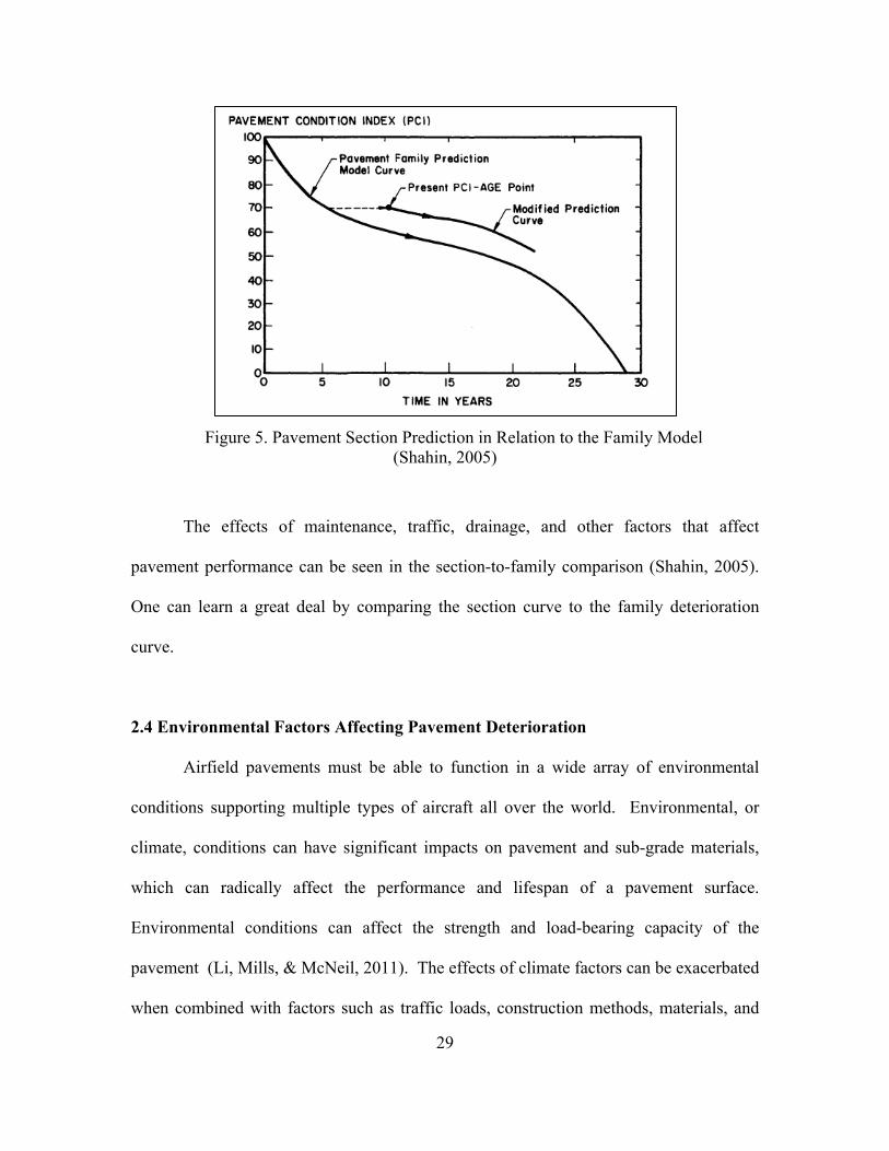
condition, regardless of age (Shahin, 2005). Figure 5 shows that a section predictive
curve, drawn through the latest PCI/age point, is parallel to the family prediction curve.
29
Figure 5. Pavement Section Prediction in Relation to the Family Model
(Shahin, 2005)
The effects of maintenance, traffic, drainage, and other factors that affect
pavement performance can be seen in the section-to-family comparison (Shahin, 2005).
One can learn a great deal by comparing the section curve to the family deterioration
curve.
2.4 Environmental Factors Affecting Pavement Deterioration
Airfield pavements must be able to function in a wide array of environmental
conditions supporting multiple types of aircraft all over the world. Environmental, or
climate, conditions can have significant impacts on pavement and sub-grade materials,
which can radically affect the performance and lifespan of a pavement surface.
Environmental conditions can affect the strength and load-bearing capacity of the
pavement (Li, Mills, & McNeil, 2011). The effects of climate factors can be exacerbated
when combined with factors such as traffic loads, construction methods, materials, and

30
M&R strategies (Li, Mills, & McNeil, 2011). The most notable environmental factors
that affect pavement performance are temperature, precipitation, subsurface-moisture,
and freeze-thaw cycles; these factors all have a major impact on long-term pavement
performance (Haas, 2001; Johanneck & Khazanovich, 2010; Li, Mills, & McNeil, 2011;
Loizos, Roberts, & Crank, 2002; Mfinanga, Ochiai, Yasufuku, & Yokota, 1996; Mills &
Andrey, 2002). Pavements are susceptible to deterioration and deformation in situations
where they are exposed to weather or climate conditions overtime. Accounting for these
effects will help pavement engineers design and manage more suitable pavements for
current climatic conditions.
2.4.1 Temperature
Temperature variations can cause damage in both flexible and rigid airfield
pavements. However, the temperature effects produce different distresses in PCC versus
AC pavements, which lead to different rates of pavement deterioration. In flexible
pavements, high and low temperatures can affect the stiffness properties of the
bituminous layers. For example, at low or freezing temperatures, asphalt becomes hard
and brittle, which can cause thermal cracking (Hironaka, Cline, & Schiavino, 2004). In
essence, the asphalt layers shrink and harden, which causes cracks to propagate through
the asphalt layers. The most common form of thermal cracking is transverse cracking.
The asphalt binder grade, age of the asphalt pavement and pavement temperature are the
primary factors affecting transverse cracking in AC pavements (Moses, Husley, &
Connor, 2009). However, most pavement engineers develop mix designs and appropriate
binders for the climate that the pavement will be constructed in.

31
Unlike asphalt pavements, Portland Cement Concretes (PCC) does not experience
the same type of distresses with high or low temperatures. Variations in temperature can
cause damage due to expansion, contraction, and slab curling. Typically, when PCC
experiences wide temperature gradients, stress and strains are introduced into the
concrete layers and result in distortions in the shape of the slab. For example, curling is
the deflection of a PCC slab due to a temperature differential through the depth of the PC
slab (ASCE). In upward curling, the edges of the slab curl upward. This is a result of the
slab surface being cooler than the slab bottom (ACSE). Repetitive trafficking of curled
slabs can cause corner cracking.
2.4.2 Precipitation and Subsurface Moisture
Precipitation and subsurface moisture is the root of many problems that affect
pavement deterioration. Moisture becomes a problem in both PCC and AC when distress
open cracks in the pavement surface allowing moisture to infiltrate the pavement and the
underlying layers potentially reducing the strength of the subgrade, base, and subbase. A
combination of moisture, heavy traffic loads, and freezing temperature can have negative
effects on the material properties, overall performance, and rate of deterioration of a
pavement network (Boudreau, Christopher, & Schwartz, 2006). High and low
temperatures can cause surfaces distress that allow water to seep into the various
pavement and subbase layers. Joints, cracks, shoulder edges, and other surface defects
provide easy access for water to penetrate into the subsurface pavement layers. Over
time, as the pavement continues to deteriorate, cracks become wider and more abundant.
This results in more moisture being allowed to penetrate into the pavement structure,

32
which leads to an accelerated deterioration rate and an increased number of moisture-
related distresses (Boudreau, Christopher, & Schwartz, 2006). Tables 1 and 2 outline
specific distresses that are caused by excessive moisture within flexible and rigid
pavements. The detrimental effects of water that has infiltrated a pavement structure are
outlined by AASHTO (1993) as:
• Reduced strength of unbounded granular materials,
• Reduced strength of subgrade soils,
• Pumping of concrete pavement with subsequent failing, cracking, and general shoulder deterioration, and
• Pumping of fines in aggregate base under flexible pavements with
resulting loss of support.
Once moisture has infiltrated a pavement structure, the capabilities, performance, and
design life will be drastically reduced. This is why moisture is one of the main
environmental factors that have significant effects on pavement deterioration.
2.4.3 Freeze/thaw weakening
Cold regions cover approximately one-third of the United States. Pavements are
subjected to freezing in the winter months and thawing in the spring. During the winter
months the load carrying capacity of the pavement increases because the pavement
structure is frozen (Janoo & Berg, 1991) In the spring months, the pavement structure
below the PCC or AC pavements thaw and can become saturated with water from the
melting ice lenses and infiltration of surface water. The saturation of the underlying
layers could reduce the strength of the base, subbase, and subgrade which, could led to an
overall reduction of bearing capacity of the entire pavement structure (Janoo & Berg,

33
1998). Freeze/thaw cycles can potentially cause spalling, scaling, and durability cracking
PCC pavements and intensify fatigue (alligator) and transverse cracking in AC
pavements. In essence, typical loading may severely damage a pavement during the
spring thaw seasons in areas prone to freeze/thaw cycles every year.
Weather and climate factors directly affect pavement performance and the rate at
which the pavement deteriorates. These factors also affect the planning, design,
construction, and maintenance and repair strategies of pavement infrastructure, both
roadways and airfields. Pavement managers must be cognizant of the climate factors that
affect their area to enable better M&R strategies for preventive maintenance of the
pavement network.

34
Table 1. Moisture Related Distresses in Flexible (AC) pavements (Boudreau, Christopher, & Schwartz, 2006)
34

35
Table 2. Moisture Related Distress in rigid (PCC) pavements (Boudreau, Christopher, & Schwartz, 2006)
35

36
2.5 Regional Climate Model
The last section of this chapter outlines the background information that was used
to develop a regional climate model for this research effort. The first section explains the
environmental factors that were used as well as the supporting information for the data.
The second section provides information pertaining to the Geospatial techniques and
tools used to create the climate model.
2.5.1 Environmental Factors for Climate Model
Relevant to the current research effort, the following two environmental factors
are explored in more detail in this section: precipitation and freezing degree-day (FDD).
The National Oceanic and Atmospheric Administration defines precipitation as “the
process where water vapor condenses in the atmosphere to form water droplets that fall to
the Earth as rain, sleet, snow, hail, etc” (NOAA, 2009). Precipitation has detrimental
effects on pavement, especially when precipitation infiltrates the lower pavement layers,
subbase, and subgrade. The second environmental factor chosen for this analysis was
freeze/thaw cycles in the form of FDD data. The Unified Facilities Criteria (UFC) 3-130-
01, General Provisions-Artic and Subartic Construction, defines FDD as “the degree-
days for any one day equal to the difference between the average daily air temperature
and 32°F.” FDD is calculated as,
𝐹𝐷𝐷 = (32− 𝑇!)
where Ta is the average daily air temperature in degrees Fahrenheit (White, 2004). An
FDD is considered positive when temperatures are below freezing and negative when
temperatures are above freezing (White, 2004). Freezing degree-days is an expression of

37
a freezing index, which is used to calculate the depth of frost penetration in pavements
and the subbase. AASHTO (1993, p. 1-25) defines the frost index as “the cumulative
effect of intensity and duration of subfreezing air temperature.”
Freezing degree-day models or temperature indices have been used successfully
to relate temperature data to frost penetration in pavement soil structures, heating
requirements for building, ice-dynamic modeling, flood forecasting, hydraulic modeling,
and snow melt modeling (Hock, 2003). According to Hock (2003, p. 104-105),
temperature index models are extremely versatile due to four reasons: “(1) general wide
availability of air temperature data, (2) relatively easy interpolation and forecasting
possibility of air temperature, (3) generally good model performance despite their
simplicity, and (4) conceptual simplicity.”
The depth of frost penetration is a vital piece of information that engineers must
know or calculate to effectively design roadway or airfield pavements in seasonal frost
regions, which experience winter temperatures that cause the ground to freeze and then
thaw during the springtime (Cortez, Kestler, & Berg, 2000). In the 1950s, the United
States Army Corps of Engineers (USACE) studied ground freezing and thawing cycles
and how these cycles affect soil properties (Bianchini & Gonzalez, 2012). These
research efforts resulted in the development of the modified Berggren (ModBerg)
equation. Cortez, Kestler, and Berg (2000, p.92) describe this equation as, “A
mathematical model that represents a one-dimensional heat flow across a moving
freezing front beneath a paved or unpaved ground surface.” However, due to the
complexity of the calculations required when using this equation, CRRL developed a tool
within the Pavement-Transportation Computer Assisted Structural Engineering (PCASE)

38
program to compute the frost penetration depth. Due to the large freeze susceptible area
within in the U.S. and the detrimental effects that freeze/thaw cycles have on pavement
performance and deterioration, FDD will be used as a primary variable for building the
regional climate zones.
2.5.2 Quantitative Spatial Analysis
Spatial analysis is a form of quantitative study that encompasses a set of
procedures to develop an inferential model that considers the spatial relationship present
in geographic data. Geospatial analysis has the ability to provide a “distinct perspective
on the world, a unique lens through which to examine events, patterns, and processes that
operate on or near the surface of our planet” (de Smith, Goodchild, & Longley, 2007).
Spatial interpolation is a spatial analysis tool that enables a user to make an estimate of a
value of a continuous field at locations where measurements have not actually been taken
(Longley, Goodchild, Maguire, & Rhind, 2011). At its core, spatial interpolation is
founded on the Tobler Law. The Tobler law states, “nearby things are more related than
distant things” (Longley, Goodchild, Maguire, & Rhind, 2011). In essence, the best way
to estimate the value for a point is to use the values from the closest observation points.
Spatial interpolation can be accomplished with the help of geographic information
system (GIS) applications to generate a continuous surface of a property (i.e.,
precipitation or temperature). Environmental Systems Research Institute’s (ERSI)
ArcInfo offers a suite of interpolation methods such as inverse distance weight (IDW)
and kriging. Longley et al (2011) describe IDW as “employing the Tobler Law by
estimating unknown measurements as weighted averages over the known measurements

39
at nearby points, giving the greatest weight to the nearest point.” In essence, IDW
provides a simple way of estimating values at locations where measurements cannot be
taken. The advantages of IDW are the simplicity of the core principles and
programming, as well as providing quick and reasonable results (Hu, 1995). The primary
disadvantage of IDW is that ambiguity may be introduced based on the choice of the
weighing factor, especially when the underlying surface characteristics are not known
and the interpolation can be effected by an uneven distribution of observed data points
(Hu, 1995).
Kriging is one of the most common spatial interpolation techniques that depends
on mathematical and statistical models. To generate a spatial interpolation surface,
kriging uses a weighted moving average method (Hu, 1995). Kriging methods rely on
the notion of autocorrelation to generate a predictive surface. Autocorrelation is a
function of distance, which is a defining feature of geostatistic techniques (ESRI, 2012).
Geostatistic techniques create a prediction surface, as well as the error or uncertainty
surfaces, associated with the predictive surface. The error provides an indication of how
good or bad the predictions are for the predictive surface.
Kriging has two distinct tasks: quantifying the spatial structure of the data and
generating a smooth predictive surface. Quantifying the surface fits a spatial-dependent
model to the observed data points. Embedded in this step, empirical semivariograms are
calculated and interpreted to explore the relationship that the Tobler Law represents. In
essence, pairs of data points that are close in distance should have a smaller difference
compared to data points that are far away from one another (ESRI, 2012).
Semivariograms measure the degree of spatial correlation between the observed data

40
points based on a function of distance and direction (Hu, 1995). The software generates
the spatial-dependent model by using the weighted least squares fit process. Kriging uses
the spatial-dependent model, the spatial data configuration, and the values of the
observed points to make a prediction for an unknown value for a specific location (ESRI,
2012).
The kriging method has its share of disadvantages. One of the main weaknesses
is that the original observation points are seldom honored, which is one of the common
problems with grid-based spatial interpolation methods (Hu, 1995). Because kriging is a
smooth interpolation technique, situations where the surface appears to be on the wrong
side of the observed data point may be observed in the generated surface. Kriging also
has potential issues with the estimation of the semivariogram. Hu (1995) states, “it is not
always easy to ascertain whether a particular estimate of the semivariogram is in fact a
true estimator of the spatial correlation in an area.”
2.6 Literature Review Summary
This chapter examined the relevant literature related to pavement management
and the associated tools and processes used to assist with the management
responsibilities. This chapter also discussed the predominant environmental factors that
can significantly affect pavement deterioration rates and pavement lifespan. Finally, this
chapter discussed the tools and techniques to develop a regional climate model for the
United States.
41
3.0 Methodology
The purpose of this chapter is to present the processes and analysis methods used
for this research effort. The methodology is a three-phased approach. The first phase
developed a four-zone regional climate model for the United States with weather data
from WeatherBank Inc. The second phase developed average rates of deterioration
models for each family pavement type that can be found on the 61 Air Force airfields
located in the United States (U.S.). The final phase of the study was a statistical
examination of the individual, regional, and overall average rate of deterioration for each
of the family of pavements.
3.1 Developing Climate Zones
Based on the literature review, precipitation, temperature, subsurface-moisture,
and freeze-thaw cycles were considered the predominant environmental factors that
significantly affect pavement deterioration and lifespan. Therefore, precipitation and
freezing degree-day (FDD) data were the two environment factors used to create the four
climate zone regions in the United States. WeatherBank Inc., a meteorological
consulting company, provided the environmental data for the research effort.
WeatherBank provides weather data and products for businesses, government agencies,
and the general public (WeatherBank, 2012). WeatherBank collects data from
approximately 1,700 National Oceanic and Atmospheric Administration (NOAA),
National Weather Service (NWS), and Federal Aviation Administration (FAA) weather

42
observation sites scattered across the U.S., Alaska, and Hawaii. Figure 6 shows the
locations of the weather stations.
Figure 6. WeatherBank U.S. Weather Station Locations
WeatherBank possesses the ability to collect hourly data for 20 different weather
parameters such as temperature, humidity, wind speed, and precipitation (WeatherBank,
2012). For this analysis, WeatherBank provided 30-year normalized precipitation and
freezing degree-day data for each of the 1,700 weather observation sites located in the
United States. WeatherBank calculates normalized data using raw weather data from
1982 through 2011. NOAA defines a “normal” of a weather variable as “the 30-year

43
average” (National Climatic Data Center, 2011). WeatherBank uses a mathematical
process to calculate the 30-year normals from daily observations from each of the
weather observations sites. The precipitation data is the total 30-year normal annual
amount of precipitation for each station in inches. Likewise, the FDD data is the FDD
calculated as a 30-year normal for each station.
To quantify the weather data to establish the four climate regions, thresholds for
the environmental factors had to be established for both precipitation and freezing
degree-days. The thresholds were established from engineering judgment and insight
from individuals at the USACE Cold Regions Laboratory and the Air Force Civil
Engineer Center. The following equation defines the wet categories:
𝑊𝑒𝑡 > 25" 𝑖𝑛 𝑝𝑟𝑒𝑐𝑖𝑝𝑖𝑡𝑎𝑡𝑖𝑜𝑛/𝑦𝑒𝑎𝑟
The following equation defines the freezing categories:
𝐹𝑟𝑒𝑒𝑧𝑒 > 750 𝐹𝐷𝐷
The precipitation and freezing degree-day data were imported into ESRI’s ArcGIS to
utilize the geospatial analysis tools to create the regional climate model.
The subsequent geospatial analysis involved combining and analyzing the
environmental geospatial data from WeatherBank. The precipitation and freezing
degree-day data were geospatially related to the location of the individual weather
stations. As stated in the previous chapter, ArcGIS has a suite of spatial analyst tools that
have the ability to create an interpolated surface from geospatially related data. Spatial
interpolation is applicable in many applications such as estimating environmental
variables (precipitation, temperature, or wind) at locations where weather stations are not
available; estimating elevation of a surface between measured locations; and estimating

44
where a contour line belongs in between two measured points (Longley, Goodchild,
Maguire, & Rhind, 2011).
To generate the climate zone model, the weather station geospatial data was
imported into ArcGIS. With the data imported, predictive surfaces were created using
the Inverse Distance Weight (IDW) and kriging geospatial interpolation techniques.
Each interpolation technique produced two surfaces, one for precipitation and one for
freezing degree-days. Using the statistical comparison feature within ArcGIS, it was
determined that the kriging method produced the most accurate interpolation surfaces for
both precipitation and freezing degree-days. To create the final climate region map, the
interpolated surfaces for precipitation and freezing degree-days were combined. This
process was executed through the "union" function in ArcMap. The "union" function
computes a geometric intersection between multiple inputs. Using this method produced
a climate model consisting of the following zones: No Freeze-Wet, No Freeze-Dry,
Freeze-Wet, and Freeze-Dry.
3.2 Developing Pavement Deterioration Rates
The Air Force Civil Engineer Center Pavements division provided the full Air
Force PAVERTM database for this effort. This database contained PCI inspection data
from the majority of the U.S. Air Force bases with an active airfield. The database
contained PCI inspection data for 61 bases scattered throughout the United States.
However, some of the more recent inspections for the bases were not yet included in the
database.

45
The database was imported into the PAVERTM program to calculate the average
linear rate of deterioration for each pavement family. All of the pavement sections
included in the PAVERTM database were categorized with the use of the family definition
tree (see Figure 2 in Chapter 1). Using the family model to categorize the pavement
sections, the average rate of deterioration for each separate type of pavement family was
produced using the prediction modeling function within the PAVERTM system. As
previously stated in Chapter 2, PAVERTM uses the “Family Method” to predict the rate of
deterioration of pavement sections. This method produces a predictive pavement
deterioration model (trend) for a family of pavements, which represents the average
behavior for the entire pavement sections associated with that particular family (Shahin,
2005). In essence, PAVERTM uses mathematical techniques to develop a best-fit curve
that produces the smallest amount of error with the constraints that (1) at age zero the PCI
is 100 and (2) the PCI can only decrease with increasing age. PAVERTM automatically
calculates the number of coefficients that produces the best-fit curve for the data set. To
get the average linear rate of deterioration for a family of pavements, the number of
coefficients must be set to two. Therefore, the slope of the line is the average rate of
deterioration for the family of pavements. This procedure was executed for every
combination of pavement from Figure 2 for each of the 61 bases in the Air Force
PAVERTM database.
3.3 Statistical Analysis
This phase of the research used Excel and the software JMP v10.0. The first goal
of this portion was to identify bases with average rates of deterioration within the

46
following sampling distribution areas: (1) plus or minus one standard deviation from the
average regional rate of deterioration, (2) more than one standard deviation greater than
the average regional rate of deterioration, and (3) more than one standard deviation less
than the average regional rate of deterioration. The second goal was to conduct an
ANOVA to determine if the climate regional average rates of deterioration for each
family of pavement are statistically different from one another.
By specifically identifying the family of pavements at individual bases with
average rates of deterioration more than one standard deviation from the regional rate of
deterioration, future research can be conducted to identify factors significantly
influencing the rate of deterioration. As discussed in Chapter 2, these factors may be
load or environmental related or may be due to the individual’s base M&R strategies.
Figure 7 shows the distribution and the associated upper and lower bounds for the regions
described above. Due to the small sample size of each family of pavements within in
each climate zone, a t-distribution was used to establish the upper and lower bounds to
help identify the distribution region for each individual bases average rate of
deterioration.

47
Figure 7. Distribution Areas
The t-distribution is a family of theoretical continuous probability distributions
similar to a normal distribution (Benson, McClave, & Sincich, 2011). The primary
difference between a normal distribution and a t-distribution is the variability, which in
the case of the t-distribution is dependent on the sample size n (Benson, McClave, &
Sincich, 2011). Using the t-distribution, a t-test statistic can be calculated to determine
the upper and lower bounds based off the degrees of freedom and the standard deviation
for each family of pavements.
The final step in the statistical analysis was to conduct an ANOVA to test the
hypothesis that the climate region rates of deterioration for each family of pavements are
statistically different from one another and different from the Air Force overall rate of
deterioration for each family of pavements. ANOVA is a statistical tool used to test for a
significant difference between two means. The validity of the ANOVA procedure is
48
based on the assumption that the population of data is normally distributed. The main
goal of the ANOVA is to determine whether or not the difference between two means can
be attributed to normal variance or to a statistical difference between the two populations
(Benson, McClave, & Sincich, 2011). Two types of variances are addressed with an
ANOVA: the “within-group variance” and the “between-group variance.” The “within-
group” variance is between the observations sampled from the same population, which is
assumed to be equal for each population. The “between-group variance” is the variance
between the means of each population being used in the comparison. Typically, the
“between-group” variance will be greater than the “within-group” variance.
Before the Student’s t-test can be executed, each family of pavements distribution
of measurements must be tested for normalcy via the Shapiro-Wilk Test. In 1965, S.S.
Shapiro and M.B. Wilk created the Shapiro-Wilk test to determine if a small random
sample comes from a normal distribution (NIST/SEMATECH, 2012). For this analysis,
the null hypothesis (Ho) states that the sample data is from a normal distribution. The
alternative hypothesis (Ha), states that the sample did not come from a normal
distribution. In this test, a W-statistic is calculated, which in the case of the JMP
software is a p-value. For example if a significance level or alpha level is set at 95%
(α=0.05) then the null hypothesis is rejected if the p-value is less than 0.05. However, if
the p-value is greater than 0.05 the null hypothesis has not been rejected, which means
the sample data came from a normal distribution. If the Shapiro-Wilk test verifies the
null hypothesis, then the Student’s t-test can be used for the pairwise comparison of the
regional rates of deterioration.

49
The JMP software executes a one-way analysis when analyzing the means from
two or more groups. To identify which pairs of means are statistically different,
individual pairwise comparisons are conducted using Student’s t-test. For the pairwise
Student t-test, the null hypothesis (Ho) states that there is no difference between a
pairwise group. The alternative hypothesis (Ha) states that the difference between
pairwise groups is statistically different. For all tests, a 95% confidence interval (α=0.05)
was applied. The Student’s t-test will generate a probability value for the t-test. If the
corresponding p-value for the Student’s t-test is less than 0.05, the null hypothesis (Ho) is
rejected. The conclusion can then be made that there is a statistical difference between
the two average rates of deteriorations being compared.
3.4 Methodology Summary
This research effort utilized a three-phased approach. The first phase focused on
constructing a regional climate model based on the predominant environmental factors
that affect pavement performance and deterioration. The second phase discussed the
process of generating the average rates of deterioration for each pavement family at each
of the bases in the PAVERTM database. The final phase discussed the statistical analysis
that was conducted at the climate region level, as well as the ANOVA that was conducted
to evaluate if a statistical difference between the climate regions exists.

50
4.0 Results and Analysis
The purpose of this chapter is to present the results of this research effort. The
chapter is organized into three main sections: Regional Climate Zone Model, Rates of
Deterioration, and Statistical Analysis. The first section discusses the results from
generating the regional climate zone models. The second section discusses the results
from calculating the average rates of deterioration for every pavement combination
outlined in Chapter 1. Finally, the results of the statistical analysis are divided into five
main subsections that discuss each climate zone and the analysis of variance (ANOVA)
results separately. To gain better insight into the results, Subject Matter Experts (SME)
at the Air Force Civil Engineer Center (AFCEC) were consulted.
4.1 Regional Climate Zone Model
The first phase of the research effort was centered on the construction of a four-
zone climate region model. The climate model consisted of the following four zones: No
Freeze-Wet, No Freeze-Dry, Freeze-Wet, and Freeze-Dry. Precipitation and freeze/thaw
cycles were the two environmental factors that were chosen for the creation of the climate
model. Using the Kriging geospatial interpolation technique, two predictive surfaces
were created from the precipitation and freezing degree-day data; Figure 8 shows the
respective interpolated surfaces.

51
Figure 8. Kriging Maps for Precipitation and Freezing Degree-Days
As stated in Chapter 3, the precipitation and freezing degree-day surfaces were combined
to develop the final climate region map. Shown in Figure 9, the final map consisted of
four zones defined by the following criteria:
• No Freeze-Wet: Precipitation > 25” and FDD < 750 • No Freeze-Dry: Precipitation < 25” and FDD < 750 • Freeze-Wet: Precipitation > 25” and FDD > 750 • Freeze-Dry: Precipitation < 25” and FDD > 750
Table 3 shows the number of bases in each of the zones. This table shows that the
numbers of bases are relatively distributed across the four zones, with a significant
number of stations in each category.
Table 3. Distribution of Air Force Bases for each Climate Zone

52
Figure 9. Climate Zone Map for the United States
52
N
l
.oo * U.S.Air Force Bases
Climate Zones
D Freeze_Dry
D Freeze_Wet
D No Freeze_Dry
No Freeze_Wet
D State Border

53
4.2 Rates of Deterioration
This section of the results discusses the average rates of deteriorations calculated
for each of the 61 bases in the database. As stated in Chapter 3, PAVER’sTM prediction
modeling function produces a best-fit curve for a particular data set. However, to
generate the average rate of deterioration for each family of pavements, the number of
coefficients was set to two to allow the prediction modeling function to generate a
straight-line trend model. Figure 10 shows an example output of the prediction modeling
function. In the figure, 0.69034 is the average rate of deterioration, which is defined as
the number of PCI points per year a particular family of pavement will deteriorate.
Figure 10. PAVERTM Prediction Modeling Output
Originally, the pavement family tree (see Figure 2 in Chapter 1) defined nine
separate families of pavements for each airfield. However, the current database did not

54
contain enough information to generate a model for each combination of pavements.
Sections of composite pavements (asphalt overlays of PCC pavements) are not as widely
used on Air Force airfields as AC or PCC pavements, which is why the database
contained minimal composite pavement sections. Therefore, the composite pavement
family did not have enough data to warrant generating deterioration models for further
analysis. Not every airfield network in the Air Force inventory contained pavement
sections from every possible combination of pavement family defined in Figure 2 in
Chapter 1. The average rates of deterioration for each region and base can be found in
Appendix B.
4.3. Statistical Analysis
This section presents the results from the statistical analysis of each of the four
climate zones as well as the comparison of the regional average rates of deterioration for
each family of pavements. As one would expect, individual airfield design varies based
on soil condition and mission aircraft as well as availability/cost effectiveness of
construction materials in different regions. Because of this fact, the number of bases with
data for each of the pavement families differs from region to region. Therefore, not every
base in a given region has data for each of the respective family of pavements associated
with the research. This will be evident in the respective rate of deterioration distribution
tables for each individual climate zones. If the average deterioration rate for a particular
pavement family at a given base, is in the upper 16% of the distribution based on the
regional average rate of deterioration, this indicates the pavements in that family at that
base are deteriorating at a higher rate than other similar pavements within the climate

55
region. On the contrary, if the average rate of deterioration for a particular family of
pavements is in the lower 16% of the distribution based on the regional average rate of
deterioration, then the pavements are deteriorating at a much slower pace than other
similar pavements within the region.
4.3.1 No Freeze-Wet Climate Region
The No Freeze-Wet Climate region consisted of 24 bases predominantly located
in the southeastern part of the United States and also the coastal areas in the states of
Washington, Oregon, and California. Table 4 shows the average rate of deterioration for
each family of pavements in this climate region. Through the use of JMP, it was
determined that all of the family of pavement distributions for this zone passed the
Shapiro-Wilk tests, i.e. the rate of deterioration of the bases within each family came
from a normally distributed population. See Appendix A for distribution graphs for each
family of pavements. Overall, the values for the average rates of deterioration are within
the expected range for pavement deterioration. Approximately 68% of the bases had
pavements from every family with an average rate of deterioration within 1 standard
deviation from the regional average except the PCC runway family (60%). Additionally,
the table indicates that AC runways are deteriorating 4 times faster than PCC for
runways. AC taxiways and aprons are deteriorating approximately 2.5-3 times faster than
the PCC pavements for taxiways and aprons. Typically, the bases place a greater
emphasis on M&R on the runway pavements. Therefore, one would expect that the
average rate of deterioration for these pavements would be relatively low. For PCC
runway pavements, this theory holds true. However, the AC runway pavements

56
experience the highest average rate of deterioration as compared to AC taxiways and
aprons.
Table 4. No Freeze-Wet Rate of Deterioration Summary Table
Tables 5 and 6 show the bases that are in the top and bottom 16%, respectively, of
the distribution in terms of the rate of deterioration for each family of pavements. As
shown in Table 5, Charleston, Dyess and Moody have rates of deterioration more than 1
standard deviation greater than the regional rate of deterioration for two of the three PCC
categories. This trend could possibly mean that these PCC pavements are experiencing
major load and environmental distresses that are different than any other base within in
the region. This climate region receives well over 25 inches of precipitation a year,
which could provide for an explanation for these bases having a higher rate of
deterioration than the regional average. Corner, diagonal transverse longitudinal
cracking, curling, warping, and pumping are all PCC distresses that potentially lead to
higher than average rates of deterioration. AC distresses such as corrugation and rutting
could be causing a higher than average rate of deterioration. Typically, corrugation and

57
rutting are distresses caused by loading effects, but both are a result of an unstable
subbase, which could be a direct result of increase moisture in the soil beneath the
pavement. Again, future research needs to be conducted to isolate the factors that are
leading to the high rate of deterioration.
Table 5. No Freeze-Wet List of Bases Above 1 Standard Deviation
Table 6. No Freeze-Wet List of Bases Below 1 Standard Deviation
From Table 6, Cape Canaveral was the only base that had an average rate of
deterioration that is in the lower 16% of the distribution based on rate of deterioration for
two PCC pavement use categories. However, this Air Force station does not have an
active flying mission and experiences very limited aircraft traffic on a regular basis,
which could be a possible explanation for the low rates of deterioration. Randolph AC
taxiway and apron pavements also show low rates of deterioration based on the analysis.
Further analysis into these bases could yield significant findings on whether or not the

58
local M&R strategies are influencing the low rate of deterioration, which then could be
applied to other bases within the region.
4.3.2 No Freeze-Dry Climate Region
The No Freeze-Dry climate region consisted of 10 bases primarily located in the
southwest part of the United States including, the southern parts of Arizona, California,
Nevada, New Mexico, and parts of Texas. Table 7 shows the average rate of deterioration
for each family of pavements in this climate region. Through the use of JMP, it was
determined that all of the family of pavement distributions for this zone passed the
Shapiro-Wilk tests. See Appendix A for distribution graphs for each family of
pavements. Overall, the values for the average rates of deterioration are within the
expected range for pavement deterioration. At least 62% of the bases had the runway
AC, taxiway PCC, and apron AC pavement families within 1 standard deviation from the
regional average. 77% of the bases had the runway PCC, taxiway AC and apron PCC
pavement families within 1 standard deviation from the regional mean. The region had at
least one or two bases that were identified as having average rates of deterioration that
categorized that particular pavement family into the top or bottom 16% of the distribution
based on average rate of deterioration. Additionally, the table indicates that runway and
taxiway AC pavements are deteriorating 4 times faster than PCC pavements for runways
and taxiways and 3 times faster than the PCC apron pavements.

59
Table 7. No Freeze-Dry Rate of Deterioration Summary Table
Tables 8 and 9 show the list of bases that are in the top and bottom 16% of the
distribution in terms of rate of deterioration in each family of pavements. From
Table 8, Nellis Air Force Base (AFB) pavements can be identified as having a rate of
deterioration in the top 16% of the distribution according to rate of deterioration for
runway and taxiway pavements. Davis-Monthan AC runway and taxiway pavement
families also show rates of deterioration well above the regional average rate of
deterioration for the same family of pavements.
Table 8. No Freeze-Dry List of Bases above 1 Standard Deviation
Table 9. No Freeze-Dry List of Bases below 1 Standard Deviation

60
Because of the climate region that Nellis and Davis-Monthan AFB are located in,
environmental distresses can lead to an increased rate of deterioration for airfield
pavements. This climate region experiences a wide range of temperatures, depending on
the time of year, and very low amounts of precipitation. During the summer months,
ambient air temperatures can climb to well over 100°F for sustained periods of time.
During the fall and winter months, temperatures can range from an average of 70°F
during the day and drop to below freezing during the night. The large temperature range
of the daily temperature cycle, especially during the winter months, can lead to
significant L/T cracking and block cracking in asphalts. The high solar radiation at these
two bases also contributes to the hardening of the asphalt pavements potentially causing
higher weathering of the asphalt binder and raveling of the aggregate in the asphalt mix.
All the above factors can lead to higher rates of asphalt pavement deterioration. Hot
temperatures can cause blowups in concrete pavements especially at joints. However,
blowups occur relatively infrequently on Air Force airfields. These are possible
explanations for the observed high rates of deteriorations from the analysis. However,
these explanations were outside the scope of the research and were not verified through
the analysis.
From Table 9, Vandenberg AFB shows low average rates of deterioration for
runway and apron PCC pavement usage categories, and March AFB shows low rates of
deterioration for AC runway and apron pavements. This trend potentially shows that
theses base have better airfield maintenance programs are working, which are driving the
low rate of deterioration. Another possible explanation could be the level of traffic for

61
the airfield is low as well. These observations need to be investigated. Keeping the rate
of deterioration low prolongs the life of the pavements, which reduces the life-cycle costs
of the pavement. Further research, must be conducted to establish exactly what trends
and factors are influencing the rates of deteriorations at the bases.
4.3.3 Freeze-Wet Climate Region
The Freeze-Wet climate region consisted of 16 bases located in states located
primary in the Midwest to the Northeast part of the United States, such as Indiana,
Maryland, Missouri, Ohio, Oklahoma, Tennessee, and Virginia. Through the JMP
analysis, 3 families of pavements did not pass the Shapiro-Wilk Test, due to statistical
outliers. See Appendix A for distribution graphs for each family of pavements. In the
PCC taxiway pavement family, the Shapiro-Wilk Test p-value (0.0255) was less than
0.05. This was mainly due to the calculated rate of deterioration for PCC taxiways at
Wright Patterson and Grissom AFBs. These outliers were identified from the box plot
from the histogram output from JMP. Figure 11 shows the histogram distribution for this
region as well as the outlier, which is represented by the small yellow square. These two
bases also showed high standard deviations (Grissom = 21.55 and Wright-Patterson =
16.989) from generating the average rate of deterioration trend model in PAVERTM
indicating considerable variation with the data for each of these bases. Once the bases
were removed, the PCC taxiway pavement family passed the Shapiro-Wilk test.

62
Figure 11. Freeze-Wet Taxiway-Concrete Distribution
Similar situations were observed in the AC Runway and PCC Apron pavement
families for this region. The AC runway pavements at Altus AFB and the PCC Apron
pavements at Grissom were flagged as statistical outliers. Altus’s AC taxiway average
rate of deterioration was 6.99 PCI points per year, which is 3 times as a high as the next
highest average rate of deterioration within this pavement family. Clearly, this rate of
deterioration is well beyond 2 standard deviations from regional mean, which means that
this rate of deterioration is heavily influencing the sample distribution. Grissom’s rate of
deterioration showed a high relatively standard deviation (Grissom = 15.457) from
generating the average rate of deterioration trend model in PAVERTM indicating
considerable variation with the data for each of these bases. Both of the distributions for
these pavement families did pass the Shapiro-Wilk test once the outliers were removed.
Table 10 shows the average rate of deterioration for each family of pavements in
this climate region. Overall, the region did have at least one or two bases that were

63
identified as having average rates of deterioration that fell in to the top or bottom 16% of
the distribution based on average rate of deterioration for each of the respective pavement
families. 70% of the bases had four out of the six pavement families within 1 standard
deviation from the regional average rate of deterioration. 60% of the bases contained the
PCC runway and taxiway pavement families within 1 standard deviation of the regional
average rate of deterioration. Additionally, the table indicates that runway AC pavements
are deteriorating 3.25 times faster than PCC pavements for runways and 2.5 times faster
than the PCC pavements for taxiways and aprons. The AC runway rate of deterioration
standard deviation among the bases was relatively higher than the rest of the pavement
categories. In the AC runway pavement family, Altus’s AC runway average rate of
deterioration was 4.79 PCI points per year, which is approximately 1.65 times higher than
the next highest rate of deterioration within this family of pavement.
Table 10. Freeze-Wet Rate of Deterioration Summary Table

64
Tables 11 and 12 show the list of bases that are in the top and bottom 16% of the
distribution in terms of rate of deterioration in each family of pavements. The bases in
this climate region are subjected to annual freeze/thaw cycles that play a substantial role
in pavement performance and could significantly influence the average rate of
deterioration. Freeze/thaw cycles can potentially cause spalling, scaling, and durability
cracking in PCC pavements and exacerbate fatigue (alligator) and transverse cracking in
AC pavements. The root cause of fatigue cracking is typically load related however,
once cracks have formed the subsequent freeze/thaw cycles can make the pavement
deteriorate at a more rapid rate. From Table 11, Wright Patterson and Tinker had two of
the three pavement usage categories fall into the top 16% of the distribution in terms of
rate of deterioration. Altus and Dover were the only bases in the AC pavement surface
categories to have rates of deterioration in the top 16% of the distribution in terms of rate
of deterioration. These airfield pavements may be experiencing load and environmental
distresses that may be different than any other base within in the region causing the rate
of deterioration to be much higher than the rest of the bases within in the region. It is
interesting to point out that the AC runway pavement at Altus were in the top 16% of the
distribution in terms of rate of deterioration. Whereas the rate of deterioration for the
PCC pavements at Altus were in the bottom 16% of the distribution in terms of rate of
deterioration. This observation raises the question of whether or not there is a potential
issue with the design or construction of the AC pavements at this location.

65
Table 11. Freeze-Wet List of Bases Above 1 Standard Deviation
Table 12. Freeze-Wet List of Bases Below 1 Standard Deviation
From Table 12, all three of the PCC pavement usage categories for Altus AFB fell into
the bottom 16% of the distribution based on average rate of deterioration. Sheppard’s
PCC runway and taxiway pavement family had a deterioration rate that is below the
regional rate of deterioration. Additionally, Whiteman’s PCC runway and apron
pavement family had a deterioration rate that is below the regional rate of deterioration.
A potential explanation of this could be the level of airfield maintenance programs
keeping the rate of deterioration at a low level. Keeping the rate of deterioration low
prolongs the life of the pavements, which reduces the cost associated with maintain the
airfield pavement network. Again, these types of observations have not been confirmed
through this research effort.
4.3.4 Freeze-Dry Climate Region
The Freeze-Dry climate region consisted of 11 bases located in the Midwest
portion of the United States including the states of Alaska, North and South Dakota,

66
Montana, Colorado, Utah, and Wyoming. Through the use of JMP, it was determined
that all of the family of pavement distributions for this zone passed the Shapiro-Wilk
tests. Table 13 shows the average rate of deterioration for each of the pavement families
in this climate region. Overall, the data for this region was distributed fairly well. At
least 70% of the bases contained five out the six pavement families with rates of
deterioration within 1 standard deviation of the regional average rate of deterioration.
66% of the bases contained the PCC apron pavement family with rates of deterioration
within 1 standard deviation of the regional average. As to be expected, there are a
number of bases with average deteriorations rate that fall into the top and bottom 16% of
distribution in terms of rate of deterioration. The AC pavements deteriorated
approximately 2.5 times faster than the PCC pavements for all three pavement usage
types in this region.
Table 13. Freeze-Dry Rate of Deterioration Summary Table

67
Tables 14 and 15 show the list of bases that are in the top and bottom 16% of the
distribution in terms of rate of deterioration in each family of pavements. Kirtland AFB
PCC taxiway and apron pavement families have been identified as having higher rates of
deterioration than the regional average. This climate region is another region that has
annual freeze/thaw cycles. As was stated for the Freeze-Wet region, the freeze/thaw
cycles can have a significant effect of the rate of deterioration for both AC and PCC
pavement families. The Elmendorf PCC Taxiway and Apron pavement families had
produced average rates of deterioration that were well below the average rate of
deterioration for those particular pavement families. These airfield networks have clearly
been identified as bases that require future research to pinpoint exactly what factors are
causing the high and low average rates of deterioration.
Table 14. Freeze-Dry List of Bases Above 1 Standard Deviation
Table 15. Freeze-Dry List of Bases Below 1 Standard Deviation

68
4.3.5 Overall Observations
Tables 16 and 17 summarize the average rates of deterioration for each climate
region. When comparing the deterioration rates of the pavement families of an individual
pavement network the apron pavements typically deteriorate at a more rapid rate than
taxiways and taxiways have deterioration rates higher than those of runways. The higher
deteriorations in aprons may be attributed to the lower load frequency (slow rolling
loads) and static loading of parked aircraft. Bases also typically place more emphasis on
M&R for runways and taxiways, which may lead to higher apron deterioration rates.
AFCEC SME’s has often observed this situation on large expanses of aprons that are not
used and not maintained. Finally, the fluids from the aircraft can cause an increased rate
of deterioration particularly when combined with heat from the Aircraft Power Units
(APU) such as the case with the B-1 bomber. This trend is clearly observed from the
values for the overall rates of deterioration. Another observation that these two tables
point out is the fact that AC pavements have a much higher rate of deterioration than
PCC pavements for the same pavement usage type. Based on the analysis AC pavements
have a deterioration rate 2.5 to 4 times higher than PCC pavements.
Table 16. Overall Climate Zone Average Rates of Deterioration-PCC

69
Table 17. Overall Climate Zone Average Rates of Deterioration-AC
Overall, the vast majority of the PCC had regional average deterioration rates
were under 0.80 PCI points per year, which at that rate it would take approximately 37
years for the pavement to reach a PCI of 70 assuming the pavement has an initial PCI of
100. The rates of deterioration for PCC pavements fall slightly below the parameters of
the conventional wisdom of having approximately a 1-2 PCI point/ year deterioration
rate. The average rate of deterioration for AC pavement families observed from this
analysis were as low as 1.7 PCI points per year to as high as 2.4 PCI points per year.
Again, these rates of deterioration fall within the parameters of conventional wisdom for
average rate of deterioration for AC pavements, which is typically 2 to 3 PCI points per
year. Based on the average rates of deterioration, the Freeze-Dry and Freeze-Wet climate
zones do have higher rates of deterioration than the No Freeze-Dry and No Freeze-Wet
zones. A potential explanation for this observation could be that the bases in the Freeze
prone regions are exposed to the annual freeze/thaw cycles and other climate conditions,
which causes an increase in the rate of deterioration. For example, in the Freeze-Dry
areas like Colorado, the daily temperature cycle and the solar radiation are relatively high
causing higher climate caused pavement stresses especially in the surface layers. In the

70
Freeze-Wet areas like Ohio, the combination of freezing and wet conditions is likely to
stress the pavement structure, which increases the rate of deterioration.
Through the rate of deterioration generation portion of the research it was
discovered that the PCI data associated with AC pavements at certain bases may have
issues with the accuracy of the age of the inspected pavement sections. In these
instances, pavement sections were observed as having ages over 40 years old with
abnormally high PCI values. These points were heavily influencing the average rate of
deterioration trend model. To eliminate the effect of this potential error, a constraint for
AC pavement age was used to only allow PAVERTM to use pavement sections with ages
less than 40 to generate the average rate of deterioration model. The accuracy of the AC
deterioration models did increase, with the age of 40 years constraint, for approximately
21% of the total AC average rate of deterioration models. This constraint was only
applied to AC pavement families and was not applied to any of the PCC pavement
families. It should be noted that for the Freeze-Wet climate zone there was not enough
data to support generating an average rate of deterioration for AC apron family of
pavements category. Because of this, the AC apron family of pavements was not
included in the following ANOVA analysis.
4.3.6 ANOVA Results
This section presents the results of the statistical analysis conducted to test if there
is a significant statistical difference between the average rate of deteriorations among the
different climatic regions for a given pavement family. This analysis was conducted
utilizing the ANOVA capabilities in the JMP software. To identify which regional

71
average rates of deterioration are statistically different from each other, a pairwise
Student’s t-test comparison was executed using JMP. For the pairwise Student t-test, the
null hypothesis (Ho) states that there are no differences between each pairwise group.
The alternative hypothesis (Ha) states that the difference between each pairwise group is
statistically different. For all tests, a 95% confidence interval (α=0.05) was applied.
Therefore, if the corresponding p-value for the Student’s t-test is less than 0.05, the null
hypothesis (Ho) can rejected and it can be concluded that there is a statistical difference
between the two average rates of deteriorations being compared. Tables 18, 19 and 20
show the Student’s t-test comparison and the corresponding p-values for the PCC
runway, taxiway and apron pavement families.
Table 18. Student's T-Test Comparison for PCC Runways

72
Table 19. Student's T-Test Comparison for PCC Taxiways
Table 20. Student's T-Test Comparison for PCC Aprons
Table 18 shows that the regional average rate of deterioration for the Freeze-Dry
runway pavement family is statistically different than the No Freeze-Wet and overall
categories. For the taxiway pavements shown in Table 19, the Freeze-Dry climate region
is statistically different than the No Freeze-Dry and No Freeze-Wet regions.
Additionally, Freeze-Wet region is statistically different than the No Freeze-Dry region.

73
For apron PCC pavements shown in Table 20, the Freeze-Dry region is statistically
different than the No Freeze-Wet, No Freeze-Dry regions and the overall apron pavement
family rate of deterioration. Overall, the Freeze-Dry region has multiple comparisons
where this zone is statistically different than the other zones for PCC pavements. A
viable explanation for this trend could be due to this climate region is prone to high
numbers of freeze/thaw cycles compared to the rest of the United States. The effects of
multiple freeze/thaw cycles could potentially cause D-cracking, scaling, or other material
related distresses, that lead to rapid deterioration without the proper maintenance. These
reasons could potentially explain why the rate of deterioration is higher or this region
compared with the rest of the regions. As seen in Table 16, the Freeze-Dry region had
the highest rate of deterioration for all three PCC pavement usage types. However, there
are many factors that affect deterioration rates besides environmental effects to include
the quality of the materials used, construction techniques, and even the initial design
could play a significant role in the deterioration rates. Typically, concrete pavements on
airfields in this climate region are designed to be able to withstand the effects of
freeze/thaw cycles. Also the construction placement techniques have been developed in
such a way as to minimize the effects that construction could potentially have on the
lifespan of the concrete slab. Therefore, without further analysis of the exact distresses
that are observed at each of these locations, it is difficult to discern whether or not the
high rates of deterioration can be full attributed to the possible environmental effects that
occur more frequently in this region than in any of the other regions.

74
From the analysis, none of the AC pavement families showed any statistical
difference for any of the pairwise comparisons. Tables 21 thru 23 show the Student’s t-
test pairwise comparisons for each of the AC pavement families. A viable explanation
for pairwise comparison returning results that show no statistical significance could be
that asphalt binders are selected to account for temperature ranges found in each
particular region within the United States. Typically, asphalt binders are selected and the
asphalt concrete mixes are designed to withstand aircraft loads and thermal loading
throughout the observed temperature range at a given location. Therefore, by design the
effects of climate are being accounted for by selecting materials that perform better in
that specific climate zone. The statistical results from this research are similar to the
results that were found from the 1990’s asphalt pavement study conducted by the Federal
Highway Administration (FHWA). The study identified that a statistical difference
between AC viscosity and temperature did not exist. The study concluded that the AC
binder for test sections of the pavements studied were properly selected for the climate
and traffic conditions.
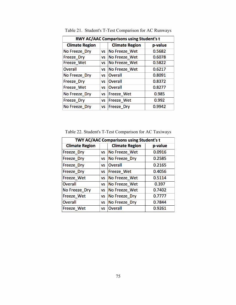
75
Table 21. Student's T-Test Comparison for AC Runways
Table 22. Student's T-Test Comparison for AC Taxiways

76
Table 23. Student's T-Test Comparison for AC Aprons
Although the analysis did not show any comparisons that were statistically
different there were still a few comparisons that had relatively low p-values. For
example, there were multiple pairwise comparisons in the taxiway and apron pavement
categories that had p-values less than 0.35. Primarily the Freeze-Dry climate region
compared to the other zones for both pavement usage categories showed relatively low p-
values. Even though the asphalt was designed for the specific region, overtime asphalt
pavements harden and become brittle with age. With age asphalt pavement becomes
susceptible to transverse cracking and block cracking which allows moisture to infiltrate
the underlying subgrade and subbase materials. Increased moisture in the underlying
layers leads to further distresses, especially in regions that are prone to freeze/thaw
cycles. These observations create the question of whether or not a statistical difference
can be found if this analysis is conducted by looking at individual climate related
distresses such as transverse cracking or raveling/weathering.

77
5.0 Conclusions and Recommendations
The purpose of this chapter is to present the conclusions of this research effort.
The chapter is organized into three main sections: Conclusions of Research, Limitations,
and Future Research. The first section addressees how the results of the study
specifically satisfy the research questions presented in Chapter 1 and layout a proof of
concept plan for this research topic. The second section address the limitations
discovered while conducting the research. The final section discusses a way ahead for
the research topic and potential future research topics.
5.1 Conclusions of Research
The primary push behind this research effort was to answer the question, “How
can climate regions, within the United States, be used to understand and quantify the
effects of climatic conditions on the deterioration rates of airfield pavements?”
Specifically, the research sought to answer the following three questions, which are
answered in detail:
1. What climatic/environmental variables should be used to develop a regional climate model for pavement deterioration modeling?
2. How do the regional climate-based average rates of deterioration for each family of pavements compare to the individual base average rates of deterioration for each family of pavements within the same region?
3. Are the regional average rates of deterioration statistically different from one another?
The first research question was centered on establishing predominant environmental
factors from the relevant literature to create a climate region model. Precipitation,

78
temperature, subsurface moisture, and freeze/thaw cycles were identified as the four
predominate factors that have a significant influence on pavement performance and
deterioration. Building an accurate climate model can be rather complex. The model
built for this research only used two environmental factors, which may have over
simplified the climate regions that exist in the United States. This model may not
account for the transition areas in between each of the zones. These transition zone areas
may not share 100% of the characteristics of one of the 4 zones.
The second research question was developed to explore the relationship between
an individual base rate of deterioration and the climate zone average regional rate of
deterioration. The main objective of this question was to identify the family of
pavements at individual bases with average rates of deterioration more than one standard
deviation from the regional rate of deterioration. This list of bases can be used for future
in-depth research/analysis to identify factors significantly influencing the rate of
deterioration. From this portion of the analysis, it was established that a number of bases
have multiple family of pavements that have rates of deterioration that fall into the top
and bottom 16% of the distribution in terms of average rate of deterioration. For
example, bases such as Charleston, Nellis, Wright-Patterson, and Moody have rates of
deterioration that were above 1 standard deviation from the regional rate of deterioration
for two of the three PCC pavement usage families. Bases such as Dyess, Davis-Monthan,
and Altus all had AC pavements that were identified as having rates of deterioration that
were 1 standard deviation above the regional rate of deterioration. This analysis also
provided a list of bases where the rate of deterioration for a particular family of
pavements was at least 1 standard deviation below the regional rate of deterioration. In

79
the PCC category, Vandenberg, March, Altus, and Elmendorf all had at least two families
of pavements meet these criteria. Altus was identified as a unique situation in which the
PCC pavements were having a low rate of deterioration but the AC pavements were
having a high rate of deterioration.
The third research question’s focus was to determine if a statistical difference
exists between the regional climate regions average rate of deterioration for each for each
family of pavements. First and foremost, the climate region average rates of deterioration
observed in both PCC and AC are all within parameters of the conventional wisdom for
average rate of deterioration for airfield pavements. Overall, the Freeze-Dry Region had
multiple comparisons where the zone is statistically different than the other zones for
PCC pavements at the 5% significance level. The PCC pavements in this climate region
are subjected to high numbers of freeze/thaw cycles when compared to the rest of the
United States. The effects of multiple freeze/thaw cycles could potentially cause
durability cracking, scaling, and other material related distresses, all which can lead to a
rapid deterioration rate without the proper execution of maintenance and rehabilitation
projects. Further analysis of the exact distress that are observed on the airfields located in
this region is needed to discern whether or not the high rates of deterioration can be fully
attributed to the possible environmental effects that occur more frequently in this region
than any of the other regions.
None of the AC pavement families showed any statistical difference for any of the
pairwise comparisons at the 5% significance level. Typically, asphalt binders are
selected and the asphalt concrete mixes are designed to withstand aircraft loads and
thermal loading throughout the observed temperature range at a given location.

80
Therefore, by design the effects of climate are being accounted for by selecting materials
that perform better in that specific climate zone.
5.2 Limitations
As with will all research, there are a varying degree of limitations; this research
effort was not an exception. Through the analysis portion of this research, limitations
were discovered with the current PAVERTM roll up data. The rollup database utilized in
the research was missing the most recent airfield PCI inspections from various
installations within the database. Approximately 32% of the bases in the database were
missing one airfield inspection and approximately 42% of the bases in the database were
missing two or more inspections from the past two decades. When the rollup database
was created, not all of the existing PCI inspections were captured in the creation of the
Air Force Airfield Pavement Rollup database. As outlined in Chapter 2, PAVERTM
generates a pavement performance predictive model that best fits the PCI data in the
database. If there is a limited amount of data associated with a particular family of
pavements, there is an increased potential for an inaccurate assessment of the true
deterioration rate for a specific pavement family to be generated. In the future, adding
the most recent inspection data to the database provides an opportunity to refine the
results and the conclusions from this research. Furthermore, building a more robust
database will provide a solid foundation for future pavement deterioration research.
Accuracy of the data is another issue/limitation that was discovered through the
analysis. In particular, the accuracy of the age of the pavement recorded during the
inspections was sometimes questionable. Observations from multiple bases proved that

81
some of the ages associated with certain inspections sections were highly inaccurate. For
example, the PCI data associated with the Seymour Johnson AFB AC runway pavements
revealed sections that are 40 years old with PCIs as high as 100. These PCI values are
not realistic for asphalt pavements, especially at that age. Inaccuracies such as this
example create additional variance within the models and result in high standard
deviations. Typically, when a prediction model has a standard deviation of error above
15 or more, there are underlying problems with the data associated with that model. The
issues that have been addressed are two of the main observed issues through the analysis.
To conduct this research in the future, these issues will have to be addressed to guarantee
the accuracy of the prediction models that PAVERTM produces and the statistical analysis
results that are based on the average rate of deterioration trend models.
First, the accuracy of the pavement sections age and the accuracy of the PCI
values for each of the inspected sections on each individual airfield need to be verified.
This process will allow for a thorough scrub of the existing data to locate and eliminate
suspect PCI data points that have the potential to heavily influence the pavement
prediction model. As discussed in the previous section, inaccurate data PCI data points do
have a significant influence on the accuracy of the prediction models that PAVERTM
produces. This step provides a solid foundation for future airfield pavement research past
the scope of this effort. The second step needs to be focused on updating the Air Force
rollup with the installation PCI surveys that are not currently in the database. Having a
complete database will allow for a more accurate assessment of the true pavement
deterioration trends at each installation, as well as at the regional and the Air Force wide
levels. The third item that needs to be explored is whether or not the full rollup database

82
can support breaking down the runway, taxiway, and aprons into primary, secondary, and
tertiary pavements. In order for PAVERTM to generate a performance predictive model,
at least five PCI data points need to exist. On most Air Force airfields, AFCEC pavement
engineers tend to see a high percentage of environmentally related distresses vice load
related distresses. However, these load related distresses tend to be observed more
frequently in the center (keel) section of the runway and taxiways as aircraft loading
tends to be concentrated in these areas. Distinguishing between deterioration cause by
load related distress, construction-related distresses, and environmental distressed would
provide greater fidelity to the analysis and reveal trends that were not evident in the
current analysis.
5.3 Future Research
The last main objective of the research was to provide a proof of concept for
conducting this type of research in the future. First and foremost, the limitations of the
rollup database must be addressed. This will ensure that the data being analyzed is the
most up-to-date and accurate. Once the database has been updated and associated data
has been scrubbed and verified, the methodology that was outlined in Chapter 3 can be
repeated to verify the results and trends of this research.
Despite the issues with the data identified in section 5.2, this effort clearly showed
that there were trends in the data for different PCC regions. While the AC analysis
showed no statistical difference between regions at the 5% significance level, the search
for an explanation of this behavior leads to several other possible research opportunities.
One potential explanation of this phenomenon was that binder selection in mix designs

83
compensates for variations in climate. Additional research could shed more light on the
validity of this hypothesis. This research also identified a number of bases that had
deterioration rates both one standard deviation above and below the mean for both PCC
and asphalt pavements. This result presents an opportunity for further research to
determine causal factors for these variations. In the case of those bases with deterioration
rates above the mean, we can identify strategies to mitigate the issues; similarly for bases
with rates below the mean, we can search for best practices that can be applied to other
bases. While the overall data shows that Air Force airfields tend to have more
environmentally related distresses than load related distresses, these differences have not
been quantified statistically; this presents another opportunity for research. Finally, this
research effort highlighted an issue with how that Air Force records
Longitudinal/Transverse (L/T) cracking distresses in AC pavements. Anecdotally,
pavement evaluators say that a high percentage of L/T cracking is due the poor
compaction on paving lane joints. L/T cracking is categorized as an environmental
distress vice a construction-related distress. This disconnect provides an opportunity to
look at avenues for more accurately recording the nature of the mechanism driving
pavement deterioration. If research identifies a better procedure, there would be greater
fidelity in the data, which would result in greater fidelity in overall trends of construction,
environmental, and load related distresses.

84
Appendix A - JMP Models
Figure 12. No Freeze-Wet Runway-PCC Distribution
Figure 13. No Freeze-Wet Runway-AC/AAC Distribution
Figure 14. No Freeze-Wet Taxiway-PCC Distribution

85
Figure 15. No Freeze-Wet Taxiway-AC/AAC Distribution
Figure 16. No Freeze-Wet Apron-PCC Distribution
Figure 17. No Freeze-Wet Apron-AC/AAC Distribution

86
Figure 18. No Freeze-Dry Runway PCC Distribution
Figure 19. No Freeze-Dry Runway AC/AAC Distribution
Figure 20. No Freeze-Dry Taxiway PCC Distribution

87
Figure 21. No Freeze-Dry Taxiway AC/AAC Distribution
Figure 22. No Freeze-Dry Apron PCC Distribution
Figure 23. No Freeze-Dry Apron AC/AAC Distribution

88
Figure 24. Freeze-Wet Runway PCC
Figure 25. Freeze-Wet Runway AC/AAC
Figure 26. Freeze-Wet Taxiway PCC (with Outliers)

89
Figure 27. Freeze-Wet Taxiway PCC (with outliers removed)
Figure 28. Freeze-Wet Taxiway AC/AAC (with outliers)
Figure 29. Freeze-Wet Taxiway AC/AAC (with outliers removed)

90
Figure 30. Freeze-Wet Apron PCC (with outliers)
Figure 31. Freeze-Wet Apron PCC (with outliers removed)
Figure 32. Freeze-Dry Runway PCC

91
Figure 33. Freeze-Dry Runway AC/AAC
Figure 34. Freeze-Dry Taxiway PCC
Figure 35. Freeze-Dry Taxiway AC/AAC

92
Figure 36. Freeze-Dry Apron PCC
Figure 37. Freeze-Dry Apron AC/AAC

93
Table 24. No Freeze-Wet Rates of Deterioration Data
Appendix B - R
ates of Deterioration T
ables
93

94
Table 25. No Freeze-Dry Rates of Deterioration Data
Table 26. Freeze-Wet Rates of Deterioration Data
94
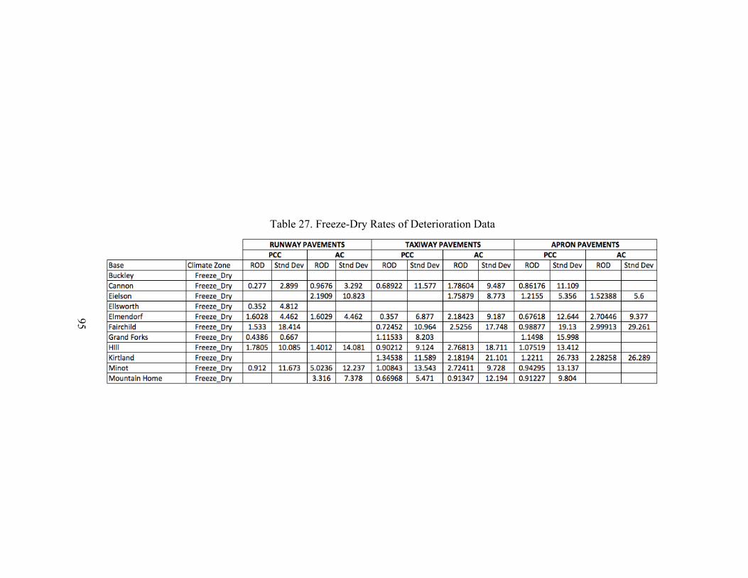
95
Table 27. Freeze-Dry Rates of Deterioration Data
95

96
References
AASHTO. (1993). AASHTO Guide for Design of Pavement Structures. Washington DC: American Association of State Highway and Transportation Officials.
Air Force Civil Engineer. (2011). 2011 U.S. Air Force Civil Engineering Strategic Plan: Build to Last...Lead the Change. Washington: HQ USAF.
American Association of State Highway and Transportation Officials. (2011). AASHTO Transportation Asset Management Guide: A Focus on Implementation. Washington DC. January 2011
Benson, P. G., McClave, J. T., & Sincich, T. (2011). Statistics for Business and Economics (Eleventh ed.). Boston, MA: Pearson.
Bianchini, A., & Gonzalez, C. R. (2012). Pavement-Transportation Computer Assisted Structural Engineering (PCASE) Implementation of the Modified Berggren (ModBerg) Equation for Computing the Frost Penetration Depth within Pavement Structures. Vicksburg, MS: U.S. Corps of Engineers Engineering Research and Development Center-Geotechnical and Structures Lab.
Boudreau, R., Christopher, B. R., & Schwartz, C. (2006). Geotechnical Aspects of Pavements. (Technical No. FHWA NHI-05-037). Washington DC: US Department of Transportation Federal Highway Administration.
Carter, A. (2013). Handling Budgetary Uncertainty in Fiscal Year 2013. Washington, DC: Department of Defense.
Chief Financial Officer. (2012). Overview- FY 2013 Defense Budget. Washington DC: Office of the Under Secretary of Defense (Comptroller).
Colorado State University. (2012). PAVER. Retrieved, 2012, from http://www.paver.colostate.edu/
Cortez, E. R., Kestler, M. A., & Berg, R. L. (2000). Computer-assisted Calculations of the Depth of Frost Penetration in Pavement Soil Structures. Transportation Systems 2000 Workshop, 92-104.
Cotts, D. G., Roper, K. O., & Payant, R. P. (2010). Facility Management Handbook (3rd Edition). New York, NY: AMACOM – Book Division of American Management Association.

97
Davit, A., Brown, R. W., & Green, J. L. (2002). U.S. Air Force (USAF) Airfield Pavement Evaluation Program. Paper presented at the 2002 Federal Aviation Administration Airport Technology Transfer Conference.
de Smith, M. J., Goodchild, M. F., & Longley, P. (2007). Geospatial Analysis: A Comprehensive Guide to Principles, Techniques and Software Tools (4th ed.). Winchelsea, UK: The Winchelsea Press.
Department of the Air Force. (1994). Airfield Pavement Evaluation Program. HQ AFCESA: AFI 32-1041. 25 April 1994
Department of the Army and Air Force. (2004). General Provisions- Artic and Subartic Construction. UFC 3-130-01. Washington DC. 16 January 2004
ESRI. (2012). ArcGIS Resources: ArcGIS Help 10.1. Retrieved 12/15, 2012, from http://resources.arcgis.com/en/help/main/10.1/index.html#/Welcome_to_the_ArcGIS_Help_Library/00qn0000001p000000/
Garamone, J. (2012). Defense Department Prepares Plans for Sequestration. American Forces Press Service. http://www.defense.gov/News/newsarticle.aspx?ID=118712. 10 December 2012
Gendreau, M., & Soriano, P. (1998). Airport Pavement Management Systems: An Appraisal of Existing Methodologies. Transportation Research Part A: Policy and Practice, 32(3), 197-214.
Gopalakrishnan, K. (2008). Neural Networks Analysis of Airfield Pavement Heavy Weight Deflectometer Data. The Open Civil Engineering Journal, 2, 15-23.
Haas, R. (2001). Reinventing the (Pavement Management) Wheel. Distinguished Lecture at Fifth International Conference on Managing Pavements, Seattle, Washington.
Haas, R., Cowe Falls, L., Macleod, D., & Tighe, S. L. (2006). Climate Impacts and Adaptations on Roads in Northern Canada. Transportation Research Board 85th Annual Meeting, Washington DC.
Hironaka, M. C., Cline, G. D., & Schiavino, C. J. (2004). Thermal Cracking of Asphalt Concrete Pavements. Maryland: MAR, Inc.
Hu, J. (1995). Methods of generating surfaces in environmental GIS applications. Paper presented at the Ersi Internatioal User Conference, Palm Springs, California.
Janoo, V. C., & Berg, R. L. (1991). Performance of Asphalt Concrete Airport Pavements During Thaw Weakening Periods. USACRREL Report, 91-97.
98
Janoo, V. C., & Berg, R. L. (1998). PCC airfield pavement response during thaw-weakening periods. Journal of Cold Regions Engineering, 12(3), 138.
Johanneck, L., & Khazanovich, L. (2010). Comprehensive evaluation of effect of climate in mechanistic-empirical pavement design guide predictions. Transportation Research Record: Journal of the Transportation Research Board, 2170(1), 45-55.
Li, Q., Mills, L., & McNeil, S. (2011). The Implications of Climate Change on Pavement Performance and Design. University of Delaware University Transportation Center.
Loizos, A., Roberts, J., & Crank, S. (2002). Asphalt pavement deterioration models for mild climatic conditions. Paper presented at the 9th International Conference on Asphalt Pavements, Copenhagen, August, 17-22.
Longley, P., Goodchild, M. F., Maguire, D., & Rhind, D. (2011). Geographic Information Systems & Science (Third ed.). Hoboken, NJ: John Wiley & Sons, Inc.
Mfinanga, D. A., Ochiai, H., Yasufuku, N., & Yokota, H. (1996). Traffic Loading and Environmental Effects on Asphalt Pavement Rutting. Memoirs-Faculty of Engineering Kyushu University, 56, 149-170.
Mills, B., & Andrey, J. (2002). Climate change and transportation: potential interactions and impacts. The Potential Impacts of Climate Change on Transportation,[US] DOT Center for Climate Change and Environmental Forecasting (Http://climate.Volpe.Dot.gov/workshop1002/mills.Doc), 77-88.
Moses, T. L., Husley, J. L., & Connor, B. (2009). Airport Manager's Guide for the Maintenance of Asphalt Pavements of General Aviation Airports. Fairbanks, Alaska: Alaska University Transportation Center.
National Climatic Data Center. (2011). NOAA's 1981-2010 Climate Normals. Retrieved January 15, 2013, from http://www.ncdc.noaa.gov/oa/climate/normals/usnormals.html#WHATARENORMALS
NIST/SEMATECH. (2012). e-Handbook of Statistical Methods. Retrieved 02/13, 2013, from http://www.itl.nist.gov/div898/handbook/
NOAA. (2009). National Weather Service. Retrieved 01/20, 2013, from http://w1.weather.gov/glossary/index.php?letter=p
Office of Asset Management. (1999). Asset Management Primer. Washington DC: Department of Transportation, Federal Highway Administration. December 1999 http://www.fhwa.dot.gov/infrastructure/asstmgmt/amprimer.pdf.

99
Sadek, A. W., Freeman, T. E., & Demetsky, M. J. (1996). Deterioration Prediction Modeling of Virgina's Interstate Highway System. Transportation Research Record, (1524), 118-129.
Shahin, M. Y. (2005). Pavement Management for Airports, Roads, and Parking Lots (Second ed.). New York, NY: Springer.
Shahin, M. Y., & Walther, J. A. (1990). Pavement Maintenance Management for Roads and Streets Using the PAVER System. Champaign, IL: U.S. Army Corps of Engineers-Construction Engineering Research Laboratory.
WeatherBank. (2012). WeatherBank, Inc. Retrieved Jan/17, 2013, from http://www.weatherbank.com/
White, K. (2004). Ice Engineering. Hanover, NH: U.S. Army Engineer Research and Development Center.

100
REPORT DOCUMENTATION PAGE Form Approved OMB No. 074-0188
The public reporting burden for this collection of information is estimated to average 1 hour per response, including the time for reviewing instructions, searching existing data sources, gathering and maintaining the data needed, and completing and reviewing the collection of information. Send comments regarding this burden estimate or any other aspect of the collection of information, including suggestions for reducing this burden to Department of Defense, Washington Headquarters Services, Directorate for Information Operations and Reports (0704-0188), 1215 Jefferson Davis Highway, Suite 1204, Arlington, VA 22202-4302. Respondents should be aware that notwithstanding any other provision of law, no person shall be subject to any penalty for failing to comply with a collection of information if it does not display a currently valid OMB control number. PLEASE DO NOT RETURN YOUR FORM TO THE ABOVE ADDRESS. 1. REPORT DATE (DD-MM-YYYY)
21-03-2013 2. REPORT TYPE Master’s Thesis
3. DATES COVERED (From – To) Aug 2011 to Mar 2013
4. TITLE AND SUBTITLE Understanding the Effects of Climate on Airfield Pavement Deterioration Rates
5a. CONTRACT NUMBER
5b. GRANT NUMBER 5c. PROGRAM ELEMENT NUMBER
6. AUTHOR(S)
Meihaus, Justin C., Captain, USAF
5d. PROJECT NUMBER If sponsor, write JON# here, or N/A if no $$. 5e. TASK NUMBER
5f. WORK UNIT NUMBER
7. PERFORMING ORGANIZATION NAMES(S) AND ADDRESS(S) Air Force Institute of Technology Graduate School of Engineering and Management (AFIT/EN) 2950 Hobson Way, Building 640 WPAFB OH 45433
8. PERFORMING ORGANIZATION REPORT NUMBER AFIT-ENV-13-M-16
9. SPONSORING/MONITORING AGENCY NAME(S) AND ADDRESS(ES) The Air Force Civil Engineer Center Mr. George Van Steenburg- AFCEC/COSC 139 Barnes Dr. Suite 1 Tyndall AFB FL 32403-5319 COMM: (850)-283-6083, DSN 523-6083, [email protected]
10. SPONSOR/MONITOR’S ACRONYM(S) AFCEC 11. SPONSOR/MONITOR’S REPORT NUMBER(S)
12. DISTRIBUTION/AVAILABILITY STATEMENT DISTRIBUTION STATEMENT A: APPROVED FOR PUBLIC RELEASE; DISTRIBUTION IS UNLIMITED
13. SUPPLEMENTARY NOTES 14. ABSTRACT Over the past two decades, pavement engineers at the Air Force Civil Engineer Center have noticed the majority of identified distresses from PCI airfield surveys are climate related. To verify these trends, a comprehensive analysis of the current airfield pavement distress database was accomplished based on a climate region perspective. A four-zone regional climatic model was created for the United States using geospatial interpolation techniques and climate data acquired from WeatherBank Inc. Once the climatic regional model was developed, the climate information for each installation was imported into the Air Force pavement distress database within PAVER. Utilizing the pavement condition prediction modeling function in PAVER, pavement deterioration models were created for every pavement family at each base in each climatic zone. This was done to generate a list of bases that may have multiple pavement families with rates of deterioration that are better or worse than the regional rates of deterioration. The average regional rates of deterioration for each pavement family were found to be within the parameters of conventional wisdom observed in Asphalt Concrete (AC) and Portland Cement Concrete (PCC). The results of the pairwise comparisons using the Student’s T-test determined the Freeze-Dry climate region deterioration rates for the PCC pavement family were statistically different than the other three regions. No significant statistical differences were observed in the AC pavement comparisons. This analysis established a foundation to investigate and identify variables causing the rates of deterioration at specific installations to differ from the regional rates of deterioration.
15. SUBJECT TERMS Pavement Condition Index, Rate of Deterioration, Airfield Pavement Distresses, Portland Cement Concrete, Asphalt Concrete
16. SECURITY CLASSIFICATION OF: 17. LIMITATION OF ABSTRACT
UU
18. NUMBER OF PAGES
113
19a. NAME OF RESPONSIBLE PERSON Alfred E. Thal, Jr., PhD
a. REPORT
U b. ABSTRACT
U c. THIS PAGE
U 19b. TELEPHONE NUMBER (Include area code) (937) 255-6565, x 7401 ([email protected])
Standard Form 298 (Rev. 8-98) Prescribed by ANSI Std. Z39-18