project number: dtz 1103 an interactive qualifying project ... · project number: dtz 1103 an...
TRANSCRIPT
I
Project Number: DTZ 1103
An Interactive Qualifying Project Report:
Submitted to the Faculty of
WORCESTER POLYTECHNIC INSTITUTE
in partial fulfillment of the requirements for the
Degree of Bachelor of Science
By
Joshua Nitso _____________________________
Kevin Woods _____________________________
Submitted April 23, 2012
Approved by Professor Dalin Tang, Project Advisor
_____________________________________________

II
ABSTRACT
The history of the stock market and selected companies within the pharmaceutical
industry were studied using the Internet and Gordon Library as primary resources. An
eight-week simulation was conducted on the stock market using different trading
techniques that were analyzed and compared for effectiveness. Using these strategies
helped develop a basic understanding of the investing world and the relative success of
different investment methods.

III
TABLE OF CONTENTS
ABSTRACT .................................................................................................................................... II
TABLE OF CONTENTS .............................................................................................................. III
TABLE OF FIGURES ....................................................................................................................V
TABLE OF TABLES .................................................................................................................. VII
1. INTRODUCTION ...................................................................................................................... 1
1.1 GOALS AND OBJECTIVES ............................................................................................... 2
1.2 GENERAL PLAN ................................................................................................................. 3
1.3 MARKET ANALYSIS ......................................................................................................... 4
1.3.1 FUNDAMENTAL ANALYSIS ..................................................................................... 4
1.3.2 TECHNICAL ANALYSIS ............................................................................................. 4
1.4 HISTORY OF STOCKS AND FINACIAL TRADING ....................................................... 5
1.4.1 BEGININGS HISTORY OF THE NYSE ...................................................................... 5
1.4.2 INDUSTRIAL AGE ....................................................................................................... 6
1.4.3 ELECTRONIC AGE ...................................................................................................... 7
1.4.4 TODAY .......................................................................................................................... 8
2. STRATEGIES........................................................................................................................... 10
2.1 DAY TRADING ................................................................................................................. 10
2.2 SHORT-TERM SWING TRADING .................................................................................. 11
2.2.1 TREND FOLLOWING ................................................................................................ 11
2.2.2 COUNTERTREND ...................................................................................................... 12
2.3 POSITION TRADING ........................................................................................................ 12
2.4 CAN SLIM .......................................................................................................................... 13
3. COMMON TOOLS .................................................................................................................. 14
3.1 MOVING AVERAGES ...................................................................................................... 14
3.1.1 SIMPLE MOVING AVERAGE .................................................................................. 15
3.1.2 EXPONENTIAL MOVING AVERAGE ..................................................................... 15
3.2 MACD ................................................................................................................................. 16
3.3 STOCHASTIC OSCILLATORS ........................................................................................ 17
4. HISTORY OF AMERICAN PHARMACEUTACAL INDUSTRY ........................................ 19
4.1 PRE-WORLD WAR I ......................................................................................................... 19
4.2 WORLD WAR .................................................................................................................... 19
4.3 WORLD WAR II ................................................................................................................ 20
4.4 1970’S – TODAY ............................................................................................................... 21
5. COMPANY HISTORIES FOR LONG-TERM INVESTMENTS ........................................... 22
5.1 PFIZER INCORPORATED (PFE) ..................................................................................... 22
5.2 MERCK & COMPANY INCORPORATED (MRK) ......................................................... 23
5.3 JOHNSON & JOHNSON (JNJ) .......................................................................................... 24
5.4 ELI LILLY AND COMPANY (LLY) ................................................................................ 26
5.5 BAXTER INTERNATIONAL INCORPORATED (BAX) ............................................... 27
6. SIMULATION 1: LONG-TERM INVESTMENTS ................................................................ 29
6.2 WEEK 1 (FEB. 7 – FEB. 12) .............................................................................................. 29
6.1.1 MONEY MARKET ACCOUNT ................................................................................. 29
6.1.2 BIG TICKET INDEX ................................................................................................... 30
6.1.3 MUTUAL FUNDS ....................................................................................................... 30

IV
6.2 WEEK 2 (FEB. 13 – FEB. 19) ............................................................................................ 31
6.3 WEEK 3 (FEB.20 – FEB. 26) ............................................................................................. 32
6.4 WEEKS 4-6 (FEB. 27 – MAR.18) ...................................................................................... 33
6.5 WEEK 7 (MAR 19.-MAR.25) ............................................................................................ 34
6.6 WEEK 8 (MAR 26 – APR.1) .............................................................................................. 35
6.7 RESULTS AND DISCUSSION ......................................................................................... 36
7. SIMULATION 2: COUNTERTRENDING ............................................................................. 39
7.1 WEEK 1 (FEB. 7 – FEB. 12) .............................................................................................. 39
7.2 WEEK 2 (FEB. 13 –FEB. 19) ............................................................................................. 47
7.3 WEEK 3 (FEB. 20 – FEB 26) ............................................................................................. 52
7.4 WEEK 4-6 (FEB. 27 – MAR. 18) ....................................................................................... 56
7.5 WEEK 7 (MAR. 19 – MAR. 25) ........................................................................................ 59
7.6 WEEK 8 (MAR. 26 – APR. 1) ............................................................................................ 62
7.7 RESULTS AND DISCUSSION ......................................................................................... 64
8. SIMULATION 3: TREND FOLLOWING .............................................................................. 67
8.1 WEEK 1 (FEB. 7 – FEB.12) ............................................................................................... 67
8.2 WEEK 2 (FEB. 13 – FEB. 19) ............................................................................................ 75
8.3 WEEK 3 (FEB. 20 – FEB 26) ............................................................................................. 84
8.4 WEEKS 4-6 (FEB. 27 – MAR.18) ...................................................................................... 89
8.5 WEEK 7 (MAR.19 – MAR.25) .......................................................................................... 92
8.6 WEEK 8 (MAR.26 – APR. 1) ............................................................................................. 93
8.7 RESULTS AND DISCUSSION ......................................................................................... 96
9. CONCLUSIONS..................................................................................................................... 102
9.1 FINAL COMPARISON OF STRATEGIES ..................................................................... 102
9.2 WHAT WE LEARNED .................................................................................................... 107
REFERENCES ........................................................................................................................... 108
V
TABLE OF FIGURES*
Figure 3.01: ABT, Weekly 1-Year Chart Example of MACD Strategies .................................... 17
Figure 7.01: JNJ, Price and Volume on February 7 ...................................................................... 40
Figure 7.02: ABT, Daily 3-Month Chart showing Volume and SMA ......................................... 40
Figure 7.03: JNJ, 1-Month Mountain Chart.................................................................................. 41
Figure 7.04: BAX, 10-Day Chart with EMA ................................................................................ 42
Figure 7.05: BCRX, Weekly 1-Year Chart with MACD.............................................................. 43
Figure 7.06: CYTR Corporation Weekly 1-Year Chart with MACD .......................................... 44
Figure 7.07: JNJ, Weekly 1-Year Chart with MACD and SMA .................................................. 45
Figure 7.08: EW, 1-Year Chart with SMA, Volume, VMA, and MACD .................................... 47
Figure 7.09: ARAY, 4-Day Chart with Volume, VMA and MACD ............................................ 48
Figure 7.10: BCRX, 15-Minute, 5-Day Chart with MACD ......................................................... 49
Figure 7.11: EW, 5-Day Chart ...................................................................................................... 49
Figure 7.12: ABT, 3-Month Chart with SMA .............................................................................. 50
Figure 7.13: LLY, 1-Month Chart with Volume and MACD....................................................... 50
Figure 7.14: XOMA, 1-Year Chart with 12-Month Forecast and 52-Week Range ..................... 51
Figure 7.15: LLY, Day Chart for February 17.............................................................................. 51
Figure 7.16: IART, 6-Month Char with SMA, Volume+, and MACD ........................................ 53
Figure 7.17: VICL, 3-Month Chart with SMA and MACD ......................................................... 54
Figure 7.18: DYAX, 3-Month Chart with SMA and MACD ....................................................... 54
Figure 7.19: JNJ, 5-Day Chart ...................................................................................................... 55
Figure 7.20: IART, 1-Month Chart with Volume ......................................................................... 56
Figure 7.21: JNJ, 7-Day Chart with EMA .................................................................................... 57
Figure 7.22: MRK, 1-Month Chart with EMA, MACD, and Fast Stochastic .............................. 58
Figure 7.23: XOMA, 5-Day Chart ................................................................................................ 58
Figure 7.24: DYAX, 5-Day Chart with EMA and Volume .......................................................... 60
Figure 7.25: CYTR, 5-Day Chart with Fast Stochastic ................................................................ 61
Figure 7.26: BAX, 5-Day Chart with MACD and Volume Average ........................................... 62
Figure 7.27: VICL, Weekly-Chart showing SMA ........................................................................ 63
Figure 7.28: Total Profit throughout Countertrending Simulation ............................................... 65
Figure 7.29: Average Countertrending Investments per Week ................................................... 66
Figure 8.01: UGLX, 1-Year Chart with EMA and Volume ......................................................... 68
Figure 8.02: KUN, 1-Year Chart with EMA and Volume ............................................................ 69
Figure 8.03: FXR, 1-Year Chart with EMA and Volume............................................................. 70
Figure 8.04: JAZZ, 1-Year Chart with EMA and Volume ........................................................... 71
Figure 8.05: DXCM, 1-Year Chart with EMA and Volume ........................................................ 72
Figure 8.06: WLP, 5-Year Chart with EMA and Volume ............................................................ 73
Figure 8.07: ARAY, 1-Year Chart with EMA and Volume ......................................................... 74
Figure 8.08: PG, 1-Year Chart with SMA and Volume ............................................................... 76
Figure 8.09: UTMD, 1-Year Chart with SMA and Volume ......................................................... 76
Figure 8.10: DVA, 1-Year Chart with SMA and Volume ............................................................ 77
Figure 8.11: IDEXX, 1-Year Chart with SMA and Volume ........................................................ 78
Figure 8.12: POZN, 1-Year Chart with SMA and Volume .......................................................... 78
Figure 8.13: MDT, 1-Year Chart with SMA and Volume ............................................................ 79
Figure 8.14: SKH, 1-Year Chart with SMA and Volume............................................................. 80

VI
Figure 8.15: TRGT, 1-Year Chart with SMA and Volume .......................................................... 80
Figure 8.16: IRIS, 1-Year Chart with SMA and Volume ............................................................. 81
Figure 8.17: FURX, 1-Year Chart with SMA and Volume .......................................................... 82
Figure 8.18: GIVN, 1-Year Chart with SMA and Volume........................................................... 82
Figure 8.19: ENSG, 1-Year Chart with SMA and Volume .......................................................... 83
Figure 8.20: ISRG, 1-Year Chart with SMA and Volume ........................................................... 85
Figure 8.21: DEPO, 1-Year Chart with SMA and Volume .......................................................... 86
Figure 8.22: UNH, 1-Year Chart with SMA and Volume ............................................................ 87
Figure 8.23: GNSZ, 1-Year Chart with SMA and Volume .......................................................... 88
Figure 8.24: VAR, 2-Month Chart with SMA and Volume ......................................................... 90
Figure 8.25: KUN, 1-Year Chart with SMA and Volume ............................................................ 91
Figure 9.1: Overall Profits for Different Trading Strategies...................................................... 102
Figure 9.2: Profits per Hour Spent for Different Trading Strategies ......................................... 103
Figure 9.3: Net Gain/Loss Transactions for Trend Following and Countertrending .................. 105
*All stock information and charts in Chapters 1-8 were taken from CNN Money, Google
Finance, or BigCharts.com.

VII
TABLE OF TABLES
Table 6.1: Week 3 Overall Long-term Stock Value ..................................................................... 32
Table 6.2: Weeks 4-6 Overall Long-term Stock Value ................................................................ 33
Table 6.3: Week 7 Overall Long-term Stock Value ..................................................................... 34
Table 6.4: Week 8 Overall Long-term Stock Value ..................................................................... 35
Table 6.5: Simulation’s Overall Long-term Stock Values............................................................ 36
Table 7.1: Week 1 Transactions and Profits ................................................................................. 46
Table 7.2: Week 2 Transactions and Profits ................................................................................. 52
Table 7.3: Week 3 Transactions and Profits ................................................................................. 56
Table 7.4: Weeks 4-6 Transactions and Profits ............................................................................ 59
Table 7.5: Week 7 Transactions and Profits ................................................................................. 61
Table 7.6: Week 8 Transactions and Profits ................................................................................. 63
Table 8.1: Week1 Transactions and Profits without Fees Included.............................................. 75
Table 8.2: Week 2 Transactions and Profits without Fees Included............................................. 84
Table 8.3: Week 3 Transactions and Profits ................................................................................. 89
Table 8.4: Week 4 Transactions and Profits ................................................................................. 92
Table 8.5: Week 5 Transactions and Profits ................................................................................. 92
Table 8.6: Week 8 Transactions and Profits ................................................................................. 95
Table 8.7: Profitable Stocks (Gainers) in Descending Order ....................................................... 97
Table 8.8: Negative Earning Stocks (losers) in Descending Order .............................................. 98
Table 8.9: Profitability of Largest Investments Compared with Smallest Investments ............. 100

1
1. INTRODUCTION
For many Americans, the stock market is merely a shadow on the horizon although one
drastically effecting their personal finances. The stock markets, or "Wall Street" as they are
collectively referred to, are often blamed sources of bad news and mill closures. By the same
token, everyone has glimpsed the vast wealth and skyrocketing financial success to be had
manipulating the worlds markets. In the past several years, the national news media has been
awash in stories about the national and global stock and financial markets. From news reports
with shocking numbers such as the $16.4 trillion loss to American households net worth's after
the housing bust or of average salaries at a Wall Street company topping two thirds of a million
dollars [1]. Even the most ignorant or uncaring citizen has certainly caught at least some of the
deluge of "Wall Street" coverage.
On a personal level, only about 54% Americans had stock market investments, the lowest
since Gallup polls began tracking in 1999 [2]. Whether driven by poor performance or by the
storm of negative press and other factors nearly half of Americans do not actively trade stocks.
That number includes, from personal experience, the vast majority of college students, who often
lack the motivation or financial backing to have stock holdings. It is therefore a reasonable
quandary, that if a student were to come into a large sum of money, they would feel suddenly
overwhelmed with the responsibility. The general “logic” of buying low and selling high tends to
govern the limited investments of this age group.
This IQP explores two distinct categories of investments for a total of five methods, all of
which are accessible to a student with a large sum of money. We have kept all of our
investments in the same industry to eliminate as much variation as possible. The first category
consists of the safety options, less likely to yield large profits but low risk and headache for an
2
investor. The profits will carry extra weight due to ease (from the investors perspective) of
attaining them. Specifically, we will analyze three longer-term investments with the first being a
deposit into a high yield money market savings account, the safest and least profitable choice we
will evaluate. Second, we will select a high performing, low cost ratio mutual fund, and
purchase a money equivalent number of stocks in this fund. The final portion of the control of
"safe investments" was to create a mini industrial average of sorts, buying one fifth of the funds
each in five of the largest market capitalization stocks in the Pharmaceutical/healthcare industry.
Purchases were restrained to one industry to eliminate some variability in the results. Companies
in the same industry tend to behave more closely than companies in very different fields.
The second category of investments is for the bolder and more active perspective trader
representing trading on a regular basis. The returns can be quite high, but the risk is entirely
dependent on the wisdom of the investor. One group member will trade with the old market
adage of "buy low and sell high.” Essentially, this trading will use charts, news and other
information to try to guess peaks and valleys in a stock price and is known officially as
countertrend investing. The second active strategy will attempt to identify established market
trends to buy into stocks and hold onto them until the trend has reversed. This strategy is known
as trend following and makes its profit from the "meat in the middle" between valleys and peaks
of trends.
1.1 GOALS AND OBJECTIVES
The objective of this IQP is to compare the general effectiveness of common investment
options and the success of longer-term versus short-term investment strategies. In the course of
this, we will develop a better understanding of the working of the current stock market and of
proper trading practice. Although there is inherent risk in investing in the stock market, this

3
project will increase our knowledge so that we will have the option to invest with better odds in
the future. We hope our final report will give the audience a background on our chosen industry
and the beginnings of stock trading in the United States. We also hope that it will improve their
knowledge of trading strategies and commonly used tools.
1.2 GENERAL PLAN
This project will start with four weeks of preparation, including current and historical
market research. Prior to the start of the simulation we will highlight the best companies for
investment using technical and fundamental analysis. The project will then consist of an eight-
week simulation of trading focused on the pharmaceutical and health services industry. The final
report will introduce key market strategies, topics and tools, along with providing historical
background for the market and characteristic companies of the health care industry that will be
used in the long-term simulation.
The premise of the simulation is that as part of a large legal settlement, both group
members have recently received substantial sums of money. After some deductions for expenses,
each is going to reserve $250,000 to actively trade within the market during the eight-week term.
There will also be $750,000 placed into a short-term trust fund only accessible at the end of the
simulations. This trust will be conservatively separated into three types of long-term
investments, such as mutual funds and certificates of deposits (CD). This will collectively create
a portfolio that will provide a control for analysis of the success of the active trading. It
represents the returns on extremely low activity and lower risk investing. The individual trading
section will utilize short-term investment strategies that offer quick turnover such as swing
trading. Both group members will exert complete control over the allocation of their $250,000.
The project will end with the final several weeks consisting of data analysis and preparation of a

4
conclusion using the results. Final results will compare the investment returns of the short-term
strategies against the low-risk, long-term investments. The conclusion will discuss the profits of
a risky, labor intensive short-term strategy and whether the returns over the control, justify the
danger.
1.3 MARKET ANALYSIS
There are two major types of market analysis. Fundamental analysis looks at the health of
industries, individual companies and of market conditions to determine the best possible
investments. Technical analysis uses data and projections of long-term, predictable market trends
to estimate the rise or fall of various stock prices. Most investment strategies use a combination
of the two forms of analysis.
1.3.1 FUNDAMENTAL ANALYSIS
Fundamental analysis is commonly taught today by schools and institutes more often than
technical analysis is covered. Fundamental analysis identifies periods of economic growth and
recession using information regarding money supply, inflation rates, debt ratios, joblessness and
consumer confidence to understand how the market works [3]. This method looks at financial
statements such as cash flows to see how efficiently capital is used as well as balance sheets,
which show a company’s assets and liabilities. Knowing this information allows one to develop
an estimate of the company’s future growth and profit potential [4].
1.3.2 TECHNICAL ANALYSIS
While fundamental analysis indicates how the economy is currently doing and which
industries are growing best, technical analysis focuses more on creating charts and following
trends. This strategy forecasts stock prices through price charts and market statistics [4]. It goes
5
off the theory that price movements are not random and that price changes are caused by an
imbalance between supply and demand [3]. The factors used by technical analysis disregard the
fundamental reasons why the stock price is changing and look for historic patterns to predict
future movements [3]. The stock market goes through ups and downs known as trends and these
trends predict when traders buy or sell under technical analysis based investing. Many
professional traders will use a combination of both fundamental and technical methods. For
example, an investor could use fundamental analysis to choose an industry or company and
technical analysis to decide when exactly to buy and sell [4].
1.4 HISTORY OF STOCKS AND FINACIAL TRADING
Stock trading began in its earliest form in Europe during the period commonly known as
the dark ages (500AD-1500AD). Towards the end of the epoch, the largest banks in Europe
began packaging the large government debts they had and selling small pieces to other banks or
to individual investors [5]. By the 1500's, some European countries had stock exchanges,
although in the strictest sense, these buildings did not trade actual shares in companies but rather
these shares of debts. As the European powers began to colonize and trade with other sections of
the world, new financial products were created [5].
1.4.1 BEGININGS HISTORY OF THE NYSE
The burgeoning trade with Asia in the in seventeenth century led to the first trading of
stocks in chartered companies. Ship captains would sell shares in voyages to the East Indies to
pay for the ship and crew up front, and in return the investor would receive a portion of the
profits if the ship did not sink. These first "corporations" did not last more than a few voyages,
but they evolved into the East Indian companies of Holland, Britain, and France [5]. These new
companies shared dividends on successful voyages and amassed large fleets and profits for
6
investors. This led to a craze in shares of similar companies and a market collapse in England
when most of the offerings turned out to be fraudulent. Crucially, because of this early panic,
stock trading was banned in the United Kingdom, a prohibition that lasted until 1825 [5].
The New York Stock Exchange, or NYSE as it is commonly abbreviated, was founded on
May 17th, 1792 by a document that became known as the Buttonwood agreement. Twenty-four
influential New York brokers signed the "agreement" under the Buttonwood tree on Wall Street
that is its namesake. A full constitution was drafted by 1817, as the New York Stock and
Exchange Board, and the name was changed to its current form in 1863. The NYSE was the
second stock exchange in the British colonies and traded in all products, especially stocks, from
the very beginning. This was an important advantage over the London brokers who were
hamstrung by the English laws forbidding stock trading [5].
Until the 20th century, the New York Exchange had little to no competition from stock
markets in the United States market. Even with little competition, the New York Exchange
suffered several market panics, including one of its largest downturns in 1879. Through stock
trading and reputation it triumphed over these issues to become by far the most important market
in the world in the 19th and 20th centuries. Many countries established national exchanges, but
these paled in volume and total market capitalization of listed companies when compared to the
NYSE. Market capitalization is the total value of all stocks existing for a said company. NYSE
did and still does, lead the entire world in total market capitalization, with the stock of its listed
companies currently worth $13.4 trillion [6].
1.4.2 INDUSTRIAL AGE
In the twentieth century, the New York Exchange ran into more issues than in the prior
century. In 1920, at the corner of Wall Street and Broad Street and near the exchange itself, a

7
horse cart packed with explosives detonated. It was the lunch hour and the streets of Manhattan
were packed with all manner of persona. When all the dust settled, the market was fixed within
days and 39 people had died [7]. It was a symbol of the market’s growing importance as a
possible scapegoat for economic troubles in popular culture. Less than ten years after the tragic
bombing the Stock Exchange and the general stock market hit the most difficult period in history
[7].
In the "Roaring Twenties", stocks increased in value four times over, an unsustainable
gain truthful only on paper. By 1933 after the crash, stocks in general were worth 80 percent less
than they were at their peak a few years earlier [8]. The banks had failed to collect on loans that
had been provided to purchase stocks, in the process of investors "buying on margin" and the
resulting consumer discomforts lead to a run on bank deposits. Banks began failing, and $160
billion in deposits was lost, all due to the original decline in the New York Stock Exchange.
Between increased regulation, the FDIC and World War II, the markets finally passed their pre-
crash highs in 1954 [8]. It had taken twenty-five years for the NSYE to recover from its mistakes
in the early twentieth century.
1.4.3 ELECTRONIC AGE
In the latter half of the century, the New York Stock Exchange was forced to deal with
the new issues of automatic trading. The computer, which had been developed by several
companies and the government during the war, grew in scope and the power of the processing
software increased yearly afterwards. By the 1980's, personal computers of usably high power
became available for the first time. A dentist in Michigan made the first online stock trade in
1983, and a new boom began. No longer did every trade have to go through a broker, and by late
decade, the companies now known as Accutrade and E-trade were performing solely online

8
trades. There were also branches of traditional brokers conducting big business online. These
online brokers evolved to offer lower cost trade fees and to offer some off-hours trading and
instant stock quotes. Anyone could now trade stocks from home, and many people now have
online accounts they used to invest. The stock exchanges also installed safeguards to prevent
computer controlled mass selloffs.
A little before the online trading boom, the NASDAQ was founded in 1971by the
National Association of Securities Dealers [9]. This new form of competition to the NYSE was
founded to be a lightning fast system, one without the burden of in-person transactions. It went
online with 2,500 securities but soon expanded. The NASDAQ revolutionized the industry and
forced the NYSE to adapt or die out [5]. Soon the fast trading, coupled with huge initial public
offerings (IPO) for newly listed companies became the standard in every market. The low fee,
fasted paced, and computer based trading had, and has opened up strategies never before
available to brokers.
1.4.4 TODAY
Today the NASDAQ is the biggest stock exchange in the world, listing on its website
that:
"Today, the NASDAQ OMX Group owns and operates 24 markets, 3
clearing houses, and 5 central securities depositories, spanning six
continents--making us the world’s largest exchange company. Eighteen
of our 24 markets trade equities. The other six trade options, derivatives,
fixed income, and commodities. We are the largest single liquidity pool
for US equities and the power behind 1 in 10 of the world’s securities
transactions. Seventy exchanges in 50 countries trust our trading

9
technology to power their markets, driving growth in emerging and
developed economies.”
The NASDAQ is a company itself and its markets boast more than 3,000 companies’
listings, many of them technology based. It has acquired important worldwide stock exchanges,
and forced the NYSE and other ancient markets to greatly expand and revolutionize their old
ways of doing business. The older markets however have adapted well and the NYSE itself is
hardly struggling. Wall Street’s market is now part of a global exchange company and its listed
companies have a total worth greater than all its competitors combined. An estimated value of
over $150 billion is traded every day within its walls or through its electronic services. In 1995,
NYSE's characteristic in person, auction style trading was supplemented by electronic trading
through hand held computers. By 2007 most stocks could be, and 80 percent of volume was,
traded through electricity [6]. There are a set number of 1,366 seats to trade on in the NYSE in
person and some seats sell for up to $3.5 million. Floor licenses without a physical seat are
much cheaper, but still expensive.
10
2. STRATEGIES
Chapter 2 discusses the different types of strategies that traders take when investing.
More specifically, day trading, short-term swing trading, position trading, and CAN SLIM
strategies will be gone over in detail.
2.1 DAY TRADING
Day traders focus on the short-term fluctuations that occur with stock prices. These
traders only work while the stock market is open, and hardly ever leave their money in stocks
overnight [4]. This method is considered very risky but offers the greatest chance of a high
reward. Due to the short time scale, fundamental analysis is practically useless. Day traders use
technical analysis and spend many daytime hours watching the stock market closely, purchasing
sometimes hundreds of different stocks a day, to work this high-stress trading method [4]. There
are two basic types of day traders – institutional and retail day traders.
Also known as market makers and specialists, institutional day traders are responsible for
maintaining inventories of securities and making sure the market for these securities are in order.
These traders are usually part of a broker firm or bank and buy and sell stock on a regular and
continual basis in order to maintain the liquidity and efficiency of listed stocks [4]. Institutional
day traders generally have better resources from the financial institution they work at, giving
them an advantage over retail day traders. Making up roughly a third of today’s trading volume,
most retail day traders work by themselves or in small groups and pay small fees to use an
electronic communications network to trade [4].
11
2.2 SHORT-TERM SWING TRADING
Swing traders hold their stocks longer than day traders, but will rarely hold stocks for
more than a few days. Similar to day trading, fundamental analysis usually offers little help with
this strategy, and is often disregarded [4]. Swing traders look at volume and liquidity, which
stocks are trending, sector selection, and volatility to make informed decisions. Swing trading
uses two types of strategies – trend following and countertrend. Trend following is used when
stocks are trending strongly and countertrend is used when a stock is range bound [4].
2.2.1 TREND FOLLOWING
Trend following is a risky strategy for investment, but offers a large opportunity for profit
[4]. Traders follow a change in the market, such as a general increase in stock price over time,
and wait for a sufficient amount of time to pass for it to be a definite trend. Once the trend is
defined, traders enter the market and ride the trend for profit. Either a constant rise in prices, or a
decline, through short selling, can be used as a trend. Trend followers ride the market through
small downturns, but exit the market and cash out their profits, if a large contrary turn occurs.
Extensive computer modeling and online trading is sometimes used under this method. A trader
sets certain conditions in the computer that when met, constitute a trend. These limits then tell
the software to buy or sell stock. Trend following also results in a large number of failing trades,
so winning investments must have enough profit to offset losses [4]. Systems settings must be
adjusted to ensure accurate trending is established before auto-trading or buyers will
automatically enter a market before a full trend develops [4]. Maximum profit can be turned by
investing entirely once a trend is established and then cashing out at the peak of the trend before
any countertrend establishes itself [4].

12
2.2.2 COUNTERTREND
Countertrend trading systems are based on intuitive market principles. The object of these
systems is to guess the bottom of a trend, or the top in the case of short selling [4]. The buyer
then sells these stocks at maximum profit at the opposite point, or at the peak of its upward trend.
Similar to trend following, computers are programmed to buy and sell stocks when they reach
pre-defined benchmarks. This strategy can be effective but is also prone to lose significant
money if current stock trends continue past a trader’s presumed turning point. Trend following
tends to outperform countertrend investing over time [4]. Day traders, swing traders, and other
investors can have limit success with contrarian investing, although a combination with trend
following is the most common investment approach. Just like in trend following, the large
number of trades can lead high transaction cost and this can ruin the profit margin, especially for
an inexperienced trader [4].
2.3 POSITION TRADING
Position traders watch movements using technical analysis to enter and leave the stock
market based on stock trends. Unlike swing and day trading, traders using this method typically
hold onto stock for several weeks or months or even years, looking to profit from a long-term
incline in stock price [10]. This system is more forgiving than the previous two described, but
also less profitable. It is much easier for traders to learn how to position trade and much less
stressful, because a general trend is being followed, rather than short ups and downs, which can
be emotionally taxing on an individual. It also requires less capital to startup and is much less
time consuming than day trading [4]. Position trading is usually something a trader will do on
the side and will not be his/her only source of income, as opposed to many day traders who rely
on the market as a primary occupation [10].
13
2.4 CAN SLIM
CAN SLIM is an investment strategy based on a formula created by William J. O'Neil, an
investor and publisher of a financial magazine. It is based on a study including the 500 top
winners in the United States market since the 1950's. The main tenant is that it supposedly
identified seven key characteristics that stocks have before they skyrocket upward. These are:
A growth of 25%-30% in quarterly per share earnings
A growth in annual earnings of at least 25%-50%
A new product or service to propel growth
A currently small overall market capitalization and volume of shares
A stock that is currently leading its sector
A stock that has institutional owners with a good profitability
A good time in the market overall, before a top and not during a downward trend of the
entire market
By investing in stocks that meet these guidelines, stockbrokers can supposedly turn large profits
by determine the next market leader. Large online and print publications compile data about
stocks that are doing well in these requirements, including the magazine published by William J.
O'Neil himself. Investors can then use these resources to pick the stocks that best meet the CAN
SLIM criteria [11].
14
3. COMMON TOOLS
Trading is a business that requires a good set of tools to be successful. This section
outlines some of the common tools used by traders. These tools will be used many times
throughout the simulations to predict trends, indicate buy/sell signals, and better understand
different aspects of the trading world.
3.1 MOVING AVERAGES
The moving average is a trading indicator that shows the direction and magnitude of a
trend over a period of time [4]. A moving average overlays the stock price data with an average
that has already occurred and traders use moving averages to trigger buy and sell signals.
Generally, when a moving averages slopes upwards, the trend is up and vice versa [4]. Two
simple tactics traders use regularly with moving averages are as follows:
Buy when the moving average slopes upward and the closing price crosses above the
moving average
Close the position when the price closes below the moving average
These two tactics only work when a stock is trending and not range bond [4]. When stocks are
traded within a confined price range, they are to be range bound, or stuck in a trading range,
trading neither higher than the high nor lower than the low during a specific time frame [4].
There are two main types of moving averages, and they are simple moving average (SMA)
and exponential moving average (EMA). SMA is used regularly by position traders to determine
exit points and EMA’s are usually applied when relying on a MACD indicator [4].

15
3.1.1 SIMPLE MOVING AVERAGE
A simple moving average calculates the average by adding all the closing prices together
and dividing by the number of prices added. Simple moving averages have the advantage of
being consistent when using the same stocks at the same time. SMA are quite simple, and
because of the way they are calculated including a long range of prices, they often do not serve
as good indicators for identifying short-term changes in a trend [4]. This is because signals take
more time to appear than the ones generated by a comparable EMA. Instead, SMAs are more
effective in determining long-term trend changes, which is the tradeoff for a potentially more
short-term reliable moving average [4]. This is because SMAs consider only a certain amount of
prices to calculate the average, and when a price is added, the last price falls off the back end.
Since all the prices are averaged using the same weight, the oldest prices affect the average just
as much as the newest prices [4].
3.1.2 EXPONENTIAL MOVING AVERAGE
An exponential moving average uses the following equation to be calculated:
EMAtoday = (Pricetoday X K) + (EMAyesterday X (1-K))
Where K = 2/ (N+1) and N = length of EMA. Unlike SMA, exponential moving averages are
not always consistent because the way the EMA is calculated depends on the starting point used.
For this reason, one website might calculate EMA significantly different than what other
websites provide [4]. This becomes a bigger problem when doing longer-term calculations,
because the problem is inflated as the data set becomes larger. In general, this is why position
traders do not use EMA. However, short-term traders often use EMA because it produces a
number closer to the current closing price, so it changes direction more rapidly, which makes it

16
more likely to signal short-term trend changes [4]. Exponential moving averages take away the
SMA problem of all prices having the same weight. Each data point affects the EMA only once
and there is no need to drop the oldest price as a new price is added. This allows the newer
prices to have a greater impact on the moving average than previous prices [4].
3.2 MACD
MACD stands for the moving average convergence divergence indicator. It is a way to
indicate momentum of a trending stock based on moving average crossovers [4]. The MACD is
calculated by subtracting a given 26-period EMA from a 12-period EMA and plotted as a line.
MACD is usually employed on weekly charts to provide better strength and direction
information than monthly or yearly charts [4].
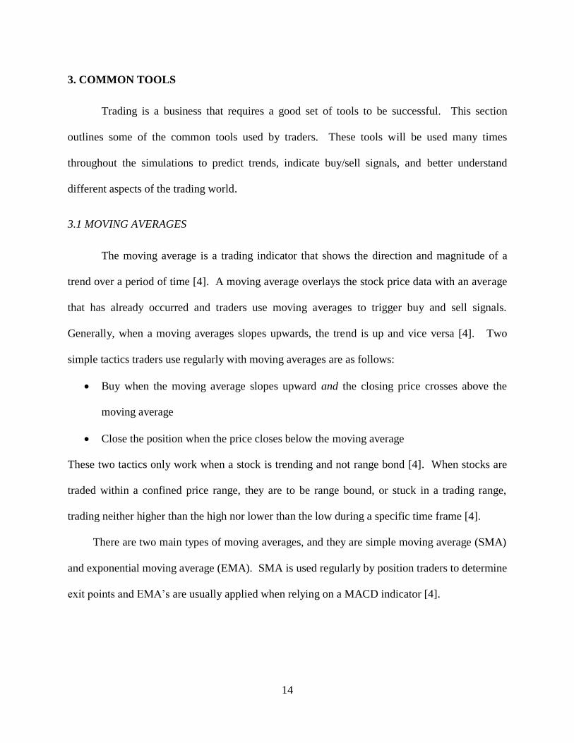
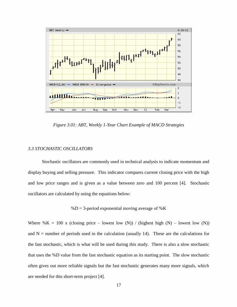
The MACD is usually drawn as two lines and a histogram below the graph as seen in
Figure 3.1. These are used by traders to predict buy and sell signals. The blue line represents the
MACD line, and when this crosses the zero mark or the signal line (indicated in red), a buy/sell
signal is given. Again, as seen in Figure 3.1, when the MACD line crosses to above the signal
line, the stock tends to increase, so the signal is to buy. Likewise, when the MACD line falls
below the signal line, a trader should likely sell the stock [4]. The MACD line can also indicate
trends. When the MACD line crosses above the center zero line, this indicates an uptrend, and
similarly, a downtrend is when the MACD line crosses below the center line [4]. The signal line
can tend to generate many false signals in short-term trading, and the MACD line is used more
by traders to determine when a stock is trending [4]. Calculating the MACD line is an important
tool in countertrend trading because it predicts that a change is about to happen, which allows
traders to more accurately guess the lows and highs of a trending stock [4].
17
Figure 3.01: ABT, Weekly 1-Year Chart Example of MACD Strategies
3.3 STOCHASTIC OSCILLATORS
Stochastic oscillators are commonly used in technical analysis to indicate momentum and
display buying and selling pressure. This indicator compares current closing price with the high
and low price ranges and is given as a value between zero and 100 percent [4]. Stochastic
oscillators are calculated by using the equations below:
%D = 3-period exponential moving average of %K
Where %K = 100 x (closing price – lowest low (N)) / (highest high (N) – lowest low (N))
and N = number of periods used in the calculation (usually 14). These are the calculations for
the fast stochastic, which is what will be used during this study. There is also a slow stochastic
that uses the %D value from the fast stochastic equation as its starting point. The slow stochastic
often gives out more reliable signals but the fast stochastic generates many more signals, which
are needed for this short-term project [4].
18
Normally, stock with a stochastic oscillator number above 80% is considered to be
“overbought” and stock that gives a number below 20% is “oversold.” When the stochastic
oscillator moves from below to above 20%, this can be taken as a signal to buy stock. Likewise,
when the stochastic number falls from above to below 80%, this can be taken as a sell signal.
Some traders additionally use a crossover strategy, which basically is where buy signals are
triggered when %K crosses over %D, and sell signals are given when %K crosses below %D.
This produces many false symbols and is less common in today’s trading world [4].

19
4. HISTORY OF AMERICAN PHARMACEUTACAL INDUSTRY
Modern day pharmaceutical corporations were not around until the early nineteenth
century. These started as large, American companies that were wholesaler/producers who
offered a full range of standard preparations [12]. In Europe, the industry started in response to
chemists’ creation of serum antitoxins and vaccines, which were based on discoveries made by
Robert Koch and Louis Pasteur.
4.1 PRE-WORLD WAR I
The isolation of the powerful opioid, morphine, in 1804 paved the way for the invention
of many modern-day medicines. Morphine was first commercially sold in 1827 by a company
called Merck, but was not widely used until the hypodermic needle was invented in 1857 [13].
The future powerhouse Pfizer came into existence in 1849, starting in New York City and
erupting to the forefront with the discovery of the antiparasitic santonin [12]. These findings,
which are still widely applicable today, took the pharmaceutical industry to a new level, setting
the stage for an explosion of industrial advancement brought on by World War I.
4.2 WORLD WAR
World War we encouraged American drug companies to invest more in research to
search for ways to develop new medicines and improve existing ones. New organizations sprung
up and existing companies became larger and more integrated. Many drugs became
commercialized during this time, such as insulin, vitamins, vaccines, and new painkillers [12].
Following World War I, the pharmaceutical industry flourished with larger scale productions of
existing drugs and new vaccines. Companies began focusing on marketing abilities to reach out
to an American public that now used drugs more than ever before [12]. These companies

20
developed into some of the largest advertisers in the nation, using NBC and CBS radio networks
to sell products to consumers [14].
4.3 WORLD WAR II
By the end of the 1940’s, World War II had accelerated the production of new antibiotics
and prescription drugs for heart and lung diseases, cancer and ulcers. In 1929, prescription drugs
accounted for only 32 percent of sold medical drugs, while by 1949 they accounted for 57
percent, and 83 percent in 1969. This period became known as the Therapeutic Revolution [12].
During this time, penicillin became a widely significant medicine in many world cultures and
prescription drugs grew rapidly across the United States. The pharmaceutical powerhouse Pfizer
ranked as one of America’s leading producers in the industry and became the first company to
commercially produce penicillin [12]. Dubbed as “wonder drugs” by the press in 1943,
antibiotics proved that bacterial infections could be treated. Penicillin was used to cure syphilis
and gonorrhea within days and treated diseases that previously would have been fatal. Other oral
antibiotics such as streptomycin and tetracyclines also fanned the nation [14]. Pharmaceutical
companies began experimenting with new antibiotics, testing them on random patients without
fully understanding the root cause of these ailments. To their amazement, the antibiotics would
often work. With the rise in over-the-counter and prescription medicines during this time, the
government began regulating drugs more strictly. This made future growth slower, marking the
1960’s as the greatest growth of the pharmaceutical companies in history [12].
Once it became involved, The Food and Drug Administration began heavily regulating
prescription drugs. At the same time many products within the industry began leveling-off so
companies started to create different brands of over-the-counter drugs for competition. They

21
also moved into developing and manufacturing new consumer chemicals including toiletries,
cosmetics, and chemically based household cleaning supplies [12].
4.4 1970’S – TODAY
In the 1970’s, a new wave of drug innovation completely restructured the medical world.
This new learning that transformed the industry was a radically new science known as molecular
biology. With this came the breakthrough of recombinant DNA and genetic engineering [12].
These inventions ignited the advancement of major pharmaceutical companies such as Eli Lilly,
Abbott, Upjohn, SmithKline, and Squibb at the time, which quickly adopted the new techniques
to rise above competition [12].
The United States currently leads the world in pharmaceuticals, placing two companies,
Pfizer and Merck in the top three in total revenues worldwide. The United States also has eleven
of the top twenty most profitable pharmaceutical companies in the world [14]. Nowadays,
Americans pay more than $200 billion annually for prescription pills, making the pharmaceutical
business one of the most profitable in the nation [14].

22
5. COMPANY HISTORIES FOR LONG-TERM INVESTMENTS
This section will outline the basic company history of eight of the major players in the
pharmaceutical industry. Many of these businesses will be used during the simulation, but they
will not be the only ones invested in.
5.1 PFIZER INCORPORATED (PFE)
Pfizer is currently the largest drug and pharmaceutical corporation in the world. The
company began in 1849 to produce chemicals for use in pharmaceutical manufacturing. This
experience as a company was invaluable to the war effort in the Second World War, as it gave
Pfizer the expertise to become a producer of newly developed antibiotics in the 1940's [12]. The
extreme wartime demand for penicillin drove the company to expand and diversify into related
fields rapidly, and the company produced half of the world’s antibiotics by 1945 [12]. The
company then became a conglomerate, producing everything from diapers to over-the-counter
cold remedies in addition to prescription drugs.
Pfizer continued to spend on research through the next several decades, although they
often acquired outsourced licenses for distribution of products developed by other companies. In
the late 20th century the company renewed its focus on the development of new drugs. In the
1980's they generated several drugs that would sell heavily in the next decade. By the 1990's the
company was spending $1.2 billion on research of new drugs each year [12].
Pfizer currently invests several billion dollars each year in research and development. In
2003 alone they invested $7.3 billion in research and development [15]. They are a market
leader in revenue, profit and market capitalization and currently market and produce such well
know drugs as Lipitor, Viagra, and Zoloft [15].

23
5.2 MERCK & COMPANY INCORPORATED (MRK)
Merck & Company Incorporated’s origins start with Friedrich Merck in Darmstadt,
Germany. He and Dr. Ernst Friedrich Schering began a small business selling pharmaceutical
products in 1851. They passed on the company to Emanuel Merck, who began the process of
creating a chemical-pharmaceutical factory that produced many different drugs and chemicals
[16]. Doing so transformed the small pharmacy into a drug manufactory. Seeing the need to
expand, Merck & Company opened its first operating building in the United States in 1891. The
building was built in New York and was a subsidiary company of E.Merck (later to be known as
Merck KGaA). In 1899, the Merck Manual of Diagnosis and Therapy was first published as a
guide for physicians and pharmacists, making the company much more eminent in the United
States. The manual became the best-selling medical textbook in history, and is still updated
annually so that physicians can continue using it [16]. A more basic home-version has been
created for the common person, and is now available in e-book, textbook and even mobile app
version.
During World War I, the company was confiscated from its German parent company and
established as an independent American business and fell under the hands of George Merck [12].
With the World Wars came the need for higher research and drug development. George Merck
lead the way in America’s germ-warfare research and established Merck’s first research
laboratories in New Jersey during the fall of 1933 [12]. To keep up with the growth of the
company, Merck merged with Powers-Weightman-Rosengarten and adopted the name Merck &
Company, Incorporated [17]. During the Second World War, Merck persevered to develop a
series of important discoveries that benefited those at the war- and home-front. Streptomycin
and cortisone were mass produced for the first time ever, by Merck & Company during the
24
1940’s, and in 1953, Merck & Company made one of its biggest advancements, by merging with
Philadelphia-based Sharp & Dohme. Soon following, in the 1960’s, Dr. Maurice Hilleman
developed the first measles and mumps vaccines and Merck introduced them to the market [17].
These developments during the mid-20th
century became ground-breaking events in medical
history.
In November of 2009, Merck merged with Schering-Plough to become the second-largest
healthcare company in the world behind only Pfizer. Schering Corporation merged with Plough,
Incorporated to create Schering-Plough Corporation in 1971, and was a leader in the
pharmaceutical industry beside Merck & Company until the merger [16]. Merck & Company
long ago passed its parent company Merck KGaA in sales, volume and revenue and now in
January of 2012, Merck is currently selling shares around $38, and has grown to a volume that is
now measured in terms of millions. This has greatly increased since January of 1970, when
Merck common stock was selling for $1.46 a share with a volume around 500,000. Merck also
had a great drop in stock price in 2009, which will be a recurring occurrence seen throughout the
paper, as many pharmaceutical companies were hit hard by the global financial crisis in the late
2000’s.
5.3 JOHNSON & JOHNSON (JNJ)
Johnson & Johnson was started in 1886 by Robert Wood Johnson and his two brothers,
James and Edward in New Jersey. In 1888, Johnson & Johnson shook the world by publishing
Modern Methods of Antiseptic Wound Treatment. It quickly became adapted across the world as
a standard teaching textbook for antiseptic surgery [18]. The book was a compilation of notes
taken by well-known doctors that had many experiences in the medical field. Also in this year,
the company manufactured the first ever first-aid kits with the intention of distribute to railroad
25
workers, but became popular across the country in treating standard injuries. Later, in the 1900’s
a First Aid manual was created to be inserted into all First Aid Kits. In the 1890’s, the brothers
turned more toward maternal needs, launching a maternity kit to make raising children more
bearable. This kit contained everything from baby clothes to safety pins. It also contained
Johnson’s Baby Powder, which was an instant hit, and became a primary product in the
development of Johnson & Johnson’s successful Baby department. Also during this time, they
released the first mass-produced sanitary napkins for women, which changed women’s health
forever [19]. In 1910, Robert Wood Johnson died, and his brother, James Wood Johnson took
over leadership of the company. During this time, BAND-AID brand adhesive bandages were
created, becoming the first bandages consumers could easily apply themselves. James Wood
Johnson expanded the company, establishing its first overseas operating building in the United
Kingdom in 1924, and growing to South America, South Africa and Australia in the early 1930’s
[18]. In 1932, Robert Wood Johnson II, son of the company founder, took over transforming the
business into a global centralized family of companies [18]. Under his control, the company
opened its first operating company in India. In the 1950’s and 1960’s, Johnson and Johnson
began acquiring many subsidiaries, including McNeil Laboratories, Cilag Chemie, and Janssen
Pharmaceutica. Robert Wood Johnson II left the company in the hands of Phillip B. Hofmann in
1963, who had a quiet thirteen years before passing on the company to James E Burke in 1976.
Burke took the company into new areas, leading the development of vision care, diabetes
management, and mechanical wound closure. He also opened the first operating companies in
China and Egypt. This was also the time that Johnson & Johnson became a founding partner in
Safe Kids Worldwide, which is a global campaign still around today, that helps reduce accidental
childhood injury [18]. In the 1990’s, Ralph S. Larsen took over as CEO, and extended the
26
company to now include the Neutrogena Corporation, Kodak’s Clinical Diagnostics business, the
Cordis Corporation, Ethicon Endo-Surgery and Centocor. In the 21st century, William C.
Weldon took over as Chairman and CEO. He is currently leading the company toward creating
medicine for people with HIV/AIDS [18]. The company celebrated its 125th
year anniversary in
2011.
In 1944, Johnson & Johnson officially went public, with a listing on the New York Stock
Exchange. Today Johnson & Johnson has over 250 subsidiaries, which was started by Robert
Wood Johnson II’s efforts to expand and globalize the company. Many famous brands were
created by these subsidiaries for Johnson & Johnson, such as Band-Aid, Benadryl, Motrin,
Neutrogena, Sudafed, Visine, and Tylenol [19]. On January 1, 1980, the stock price of Johnson &
Johnson was only $1.65 and the volume was 715,200 [20]. According to CNN.com, stock prices
have greatly increased to over $45 a share for the past five years, and on January 3, 2012, the
stock price of Johnson & Johnson recorded a high of $65.93 and currently has a market cap of
$170 billion, dwarfing the numbers the company produced in 1980. The company recorded over
$65 billion in net revenues during 2011, and has been placed in the top 3 pharmaceutical
companies in the world by CNN, Fortune, and Barron’s Magazine. Johnson & Johnson’s main
competitors are Pfizer Incorporated, Novartis AG, and Merck & Company Incorporated
5.4 ELI LILLY AND COMPANY (LLY)
Eli Lilly and Company was started in 1876 in Indiana by Colonel Eli Lilly, a
pharmaceutical chemist and veteran of the Civil War [21]. In 1923, Lilly produced the world’s
first commercial insulin product, Iletin, to help people with diabetes, which at the time was a
deadly disease. In the 1950’s, Lilly launched the antibiotics, erythromycin and vancomycin,
which expanded the antibiotic world for patients allergic to penicillin and for penicillin-resistant

27
bacteria [21]. Lilly made a big breakthrough in the 1980’s, producing Prozac, the first major drug
for clinical depression. Prozac is still a major drug today with over 25 million prescriptions
given in 2010 alone [21]. In the 21st century, Lilly has focused heavily on creating treatments for
Bipolar disorder and improving the life of diabetics. In 1978, Eli Lilly and Company went
public, selling shares for $2.40 a piece. Since then, the stock price has been as high as $95, and
today run around $40 a share [6].
5.5 BAXTER INTERNATIONAL INCORPORATED (BAX)
Baxter is a pharmaceutical and medical supplies manufacturer based in Illinois.
Internally, it is segmented into three divisions. A bio science division focuses on genetic
medicine, new vaccines, and biological sealants and products for surgical procedures, accounting
for 45% of corporate revenue. Baxter’s medical division produces syringes and inhaled
anesthetic, and accounts for about 35% of annual revenue. The rest of its product line includes
home dialysis, regenerative medicine and anti-nausea products. The company showed an 8.18%
sales growth in 2011, and had total sales of just under $14 billion. This contains an estimated
$7.05 billion profit, although a price to sales ratio of 2.34 puts it under the industry average [22].
Historically Baxter was founded in 1931 to distribute intravenous solutions manufactured
by its namesake, Dr. Donald Baxter. The company went public in 1951, and had become the
world’s largest hospital supplier by 1985. It had immense success with the selling the first home
portable dialysis machine. In 1992 it controlled an insurmountable 75% of the dialysis market. It
has diversified lately into selling equipment both to aid surgical procedures, and medical devices.
In the first decade of the 21st century, the company has hit more unfortunate straits, and despite
continued growth, it has been subject to several major FDA warnings, seizures and injunctions

28
[22]. Similar to many other businesses in the pharmaceutical industry, Baxter showed a great
increase in stock price just before the crash in 2009.
29
6. SIMULATION 1: LONG-TERM INVESTMENTS
In this chapter, we looked into many different types of safer, low activity investments.
These represent ways to use the time value of money to your advantage while also not having to
take huge risks within the market. Each of the three types of investments is a category general
regarded as safer and easier than playing on the open stock market.
6.2 WEEK 1 (FEB. 7 – FEB. 12)
This is the first week of simulation. Trading was started on Tuesday, February 8 by both
members. Not many profits have been seen yet because they were just established this week and
we will not be observing profits for analysis until the second week of simulations.
6.1.1 MONEY MARKET ACCOUNT
A money market savings account is a type of account managed by a normal bank or
credit union. These accounts generally pay a much higher interest rate than normal savings
accounts but have more restrictive terms. For example, the money market account we chose to
invest in was offering a weekly interest of 1% whereas normal FDIC insured accounts pay out at
a whopping .25% interest rate. Thereby, there is much more money to be had in our situation,
where money is sitting for 8 weeks, in a money market account. The account we picked was the
Incredible Money Market account, from the online bank know as Incredible Bank. We invested
the maximum $250,000 on Tuesday, February 7th, at the nominal interest rate of 1%. The
account pays interest weekly and has a ten-dollar monthly fee. The restrictions that allow the
higher interest rate are a minimum balance of $2,500 and no more than six transactions per
month. None of the restrictions are an issue in the scope of the project. The yield for the

30
account is fixed, and we can calculate our returns at the end of the simulation correctly right
now.
6.1.2 BIG TICKET INDEX
One of the general trends is that the stock market tends to raise over time, especially blue
chip stocks. Warren Buffet has repeatedly mentioned it in his essays about his investing with
Berkshire Hathaway [23]. So, with the advice of the average Joe wanting to buy in companies
he has heard of, and hoping for the gradual increase of such high market capitalization stocks, we
sought a small package of equation stakes in the largest companies. It is sort of a very limited
sample healthcare industry national average, and is entirely composed of five companies each
capitalized over $50 billion. We have purchase roughly $50,000 of stock in each of the five on
Tuesday, February 7th. Specifically, we own 769 shares of Johnson and Johnson, along with
2,387 shares of Pfizer, and 1,307 shares of Merck, 1,266 shares of Eli Lilly, and 881 shares of
Baxter.
6.1.3 MUTUAL FUNDS
The final option we chose was to have someone else, who is hopefully knowledgeable,
invest for us. Hiring a broker is outside the scope and cost of this project, so our options were
limited. What appealed to us most was to invest into a managed mutual fund, to buy stocks in a
paper creation, and receive a tiny sliver of the thousands of investments contained in a large
fund. Most mutual funds operate on an expense ratio, which is a certain percentage of the
holdings in a fund taken every year to cover management and administration cost. This fee is the
price to buy a small sliver of the whole large portfolio of stocks in a mutual fund.
To select the best mutual fund, we looked across several lists best performing funds to
select those worthy of further investigation. Every mutual fund we screened was a health care/

31
pharmaceutical or health services based fund. A chart was constructed for easy comparison,
which looked at 2011 annual returns, the current share price, the Morningstar risk rating, the total
fund asset size, and also the fund expense ratios. We looked for a fund with a low risk rating and
a large asset size, for stability and to limit the potential for catastrophe. We wanted a fund that
had done well recently and had shown a good annual percent return in 2011. Most importantly,
we tried to select a fund with a low expense ratio, as that represents fixed fee that are removed
from an account whether it does well or not. A high expense ratio can make a fund with a
dazzlingly return percentage lose money for an investor.
Considering carefully all these factors, we choose to purchase $250,000 worth of shares
in Fidelity Select Healthcare. It was by far the largest we considered, and had a medium risk
rating coupled with a very low, the second lowest overall expense ratio. Its expense ratio of
.82%, on an account with nearly $2.2 billion in assets amounted to less than a third of the ratios
for some of the other accounts. The well-known brand name of Fidelity and the well above
average2011 annual return of 16.96% made it the clear choice. The final purchase on Tuesday
February 7th consisted of 1,881 stocks, purchased at $132.88 apiece, with less than $100 of the
original amount left as a remainder. The stock symbol is FSPHX.
6.2 WEEK 2 (FEB. 13 – FEB. 17)
The first week of simulation was a negative for the industry leaders, and four of the five
big ticket stocks we selected to hold onto for the simulation lost money in their first week. As the
week went on, the stocks recovered. The second week of trading was vastly more beneficial to
the long-term account, and four of the five stocks gained value. The end of the week totals, in
descending order of profit; Pfizer, with $572.88 gained overall, Merck with $405.17 gained,
Johnson and Johnson with $292.31 in gains, and finally, Baxter with a gain of $237.87. Eli Lilly
32
was losing well over a $1,000 off its cost basis mid-week, its stock finally ended a multi-week
tumble and recovered late week to achieve losses of only $303.84 overall.
The Mutual fund remained mostly stagnant, losing $.33 per share overall since the shares
were purchased. This resulted in a final loss of the first two weeks of $620.73. Because this fund
is dependent on one share, it is very susceptible to even small decreases in value.
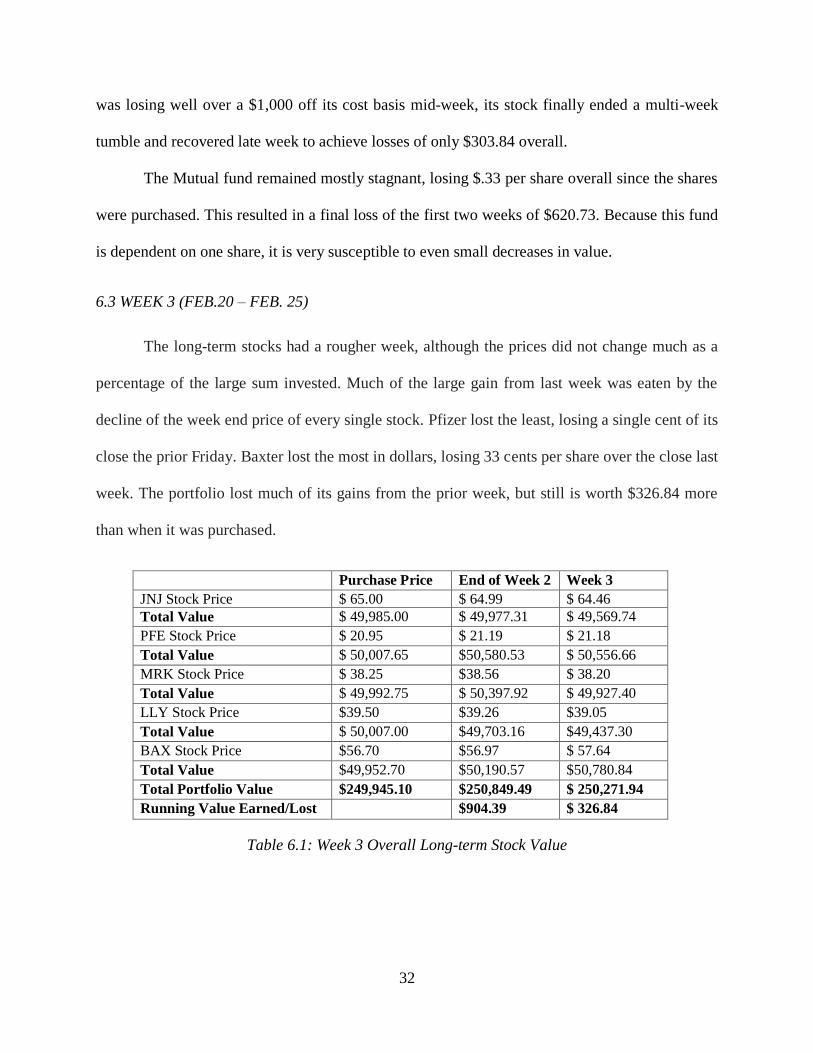
6.3 WEEK 3 (FEB.20 – FEB. 25)
The long-term stocks had a rougher week, although the prices did not change much as a
percentage of the large sum invested. Much of the large gain from last week was eaten by the
decline of the week end price of every single stock. Pfizer lost the least, losing a single cent of its
close the prior Friday. Baxter lost the most in dollars, losing 33 cents per share over the close last
week. The portfolio lost much of its gains from the prior week, but still is worth $326.84 more
than when it was purchased.
Purchase Price End of Week 2 Week 3
JNJ Stock Price $ 65.00 $ 64.99 $ 64.46
Total Value $ 49,985.00 $ 49,977.31 $ 49,569.74
PFE Stock Price $ 20.95 $ 21.19 $ 21.18
Total Value $ 50,007.65 $50,580.53 $ 50,556.66
MRK Stock Price $ 38.25 $38.56 $ 38.20
Total Value $ 49,992.75 $ 50,397.92 $ 49,927.40
LLY Stock Price $39.50 $39.26 $39.05
Total Value $ 50,007.00 $49,703.16 $49,437.30
BAX Stock Price $56.70 $56.97 $ 57.64
Total Value $49,952.70 $50,190.57 $50,780.84
Total Portfolio Value $249,945.10 $250,849.49 $ 250,271.94
Running Value Earned/Lost $904.39 $ 326.84
Table 6.1: Week 3 Overall Long-term Stock Value
33
The mutual fund gained back all of its losses from the prior week, and even gained 3
cents over the original purchase price. It is price currently sits at $132.91. The total value gained
over the purchase price was $56.43. The fund recovered from a prior week loss of $620.73.
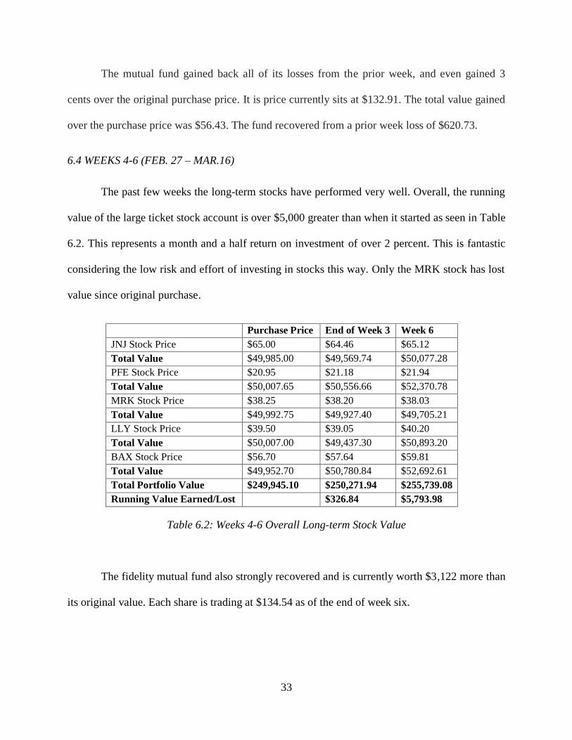
6.4 WEEKS 4-6 (FEB. 27 – MAR.16)
The past few weeks the long-term stocks have performed very well. Overall, the running
value of the large ticket stock account is over $5,000 greater than when it started as seen in Table
6.2. This represents a month and a half return on investment of over 2 percent. This is fantastic
considering the low risk and effort of investing in stocks this way. Only the MRK stock has lost
value since original purchase.
Purchase Price End of Week 3 Week 6
JNJ Stock Price $65.00 $64.46 $65.12
Total Value $49,985.00 $49,569.74 $50,077.28
PFE Stock Price $20.95 $21.18 $21.94
Total Value $50,007.65 $50,556.66 $52,370.78
MRK Stock Price $38.25 $38.20 $38.03
Total Value $49,992.75 $49,927.40 $49,705.21
LLY Stock Price $39.50 $39.05 $40.20
Total Value $50,007.00 $49,437.30 $50,893.20
BAX Stock Price $56.70 $57.64 $59.81
Total Value $49,952.70 $50,780.84 $52,692.61
Total Portfolio Value $249,945.10 $250,271.94 $255,739.08
Running Value Earned/Lost $326.84 $5,793.98
Table 6.2: Weeks 4-6 Overall Long-term Stock Value
The fidelity mutual fund also strongly recovered and is currently worth $3,122 more than
its original value. Each share is trading at $134.54 as of the end of week six.
34
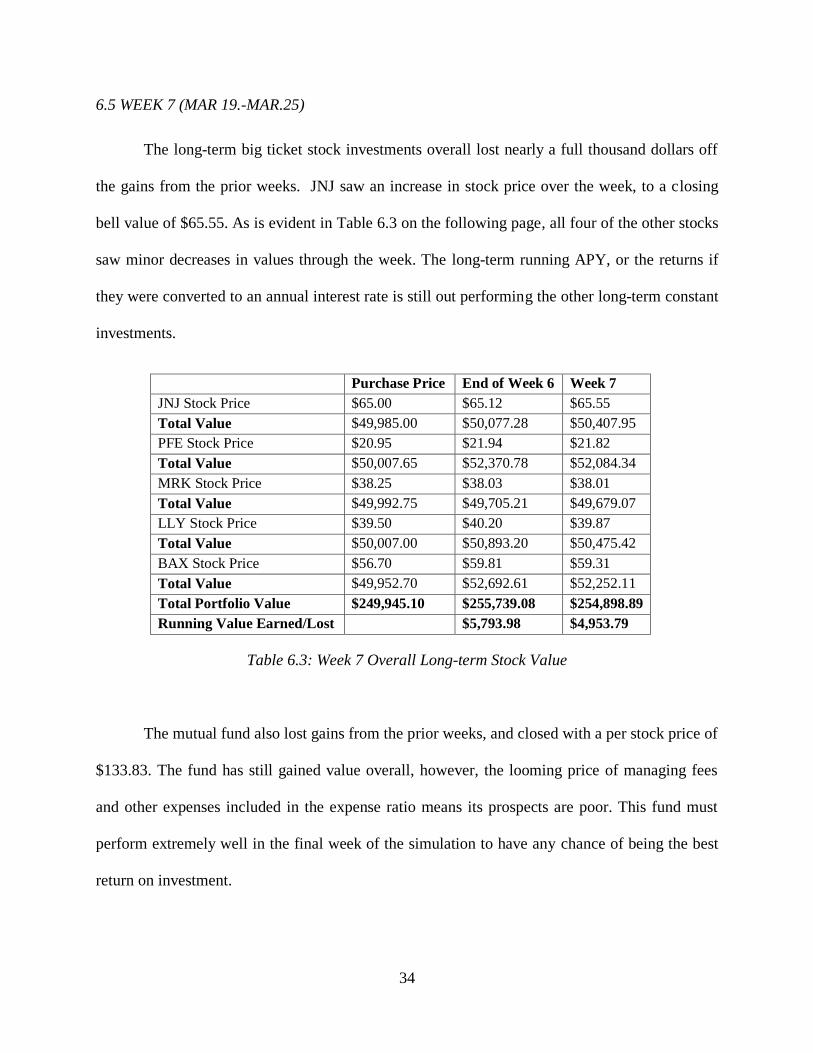
6.5 WEEK 7 (MAR 19.-MAR.25)
The long-term big ticket stock investments overall lost nearly a full thousand dollars off
the gains from the prior weeks. JNJ saw an increase in stock price over the week, to a closing
bell value of $65.55. As is evident in Table 6.3 on the following page, all four of the other stocks
saw minor decreases in values through the week. The long-term running APY, or the returns if
they were converted to an annual interest rate is still out performing the other long-term constant
investments.
Purchase Price End of Week 6 Week 7
JNJ Stock Price $65.00 $65.12 $65.55
Total Value $49,985.00 $50,077.28 $50,407.95
PFE Stock Price $20.95 $21.94 $21.82
Total Value $50,007.65 $52,370.78 $52,084.34
MRK Stock Price $38.25 $38.03 $38.01
Total Value $49,992.75 $49,705.21 $49,679.07
LLY Stock Price $39.50 $40.20 $39.87
Total Value $50,007.00 $50,893.20 $50,475.42
BAX Stock Price $56.70 $59.81 $59.31
Total Value $49,952.70 $52,692.61 $52,252.11
Total Portfolio Value $249,945.10 $255,739.08 $254,898.89
Running Value Earned/Lost $5,793.98 $4,953.79
Table 6.3: Week 7 Overall Long-term Stock Value
The mutual fund also lost gains from the prior weeks, and closed with a per stock price of
$133.83. The fund has still gained value overall, however, the looming price of managing fees
and other expenses included in the expense ratio means its prospects are poor. This fund must
perform extremely well in the final week of the simulation to have any chance of being the best
return on investment.

35
6.6 WEEK 8 (MAR 26 – APR.1)
During the final week of the simulation, the Big Ticket stocks finished strong. For the
first time, every single stock had gained value. When the stocks were sold at their Friday closing
price to end the simulation, MRK saw a profit of $196.05, LLY a profit of $974.82, JNJ a profit
of $1,038.24, and BAX with a profit of $2,713.48. PFE produced a very large final profit of
$4,057.90, the largest of the group. The stocks resurged after a poor week seven to their highest
overall level, just in time for the final sale. The figures for the current week, the previous week,
and the beginning of the simulation can be seen in Table 6.4.
Purchase Price End of Week 7 Week 8
JNJ Stock Price $ 65.00 $ 65.55 $ 65.96
Total Value 49,985.00 $ 50,407.95 $ 50,723.24
PFE Stock Price $ 20.95 $ 21.82 $ 22.65
Total Value $ 50,007.65 $ 52,084.34 $ 54,065.55
MRK Stock Price $ 38.25 $ 38.01 $ 38.40
Total Value $ 49,992.75 $ 49,679.07 $ 50,188.80
LLY Stock Price $ 39.50 $ 39.87 $ 40.27
Total Value $ 50,007.00 $ 50,475.42 $ 50,981.82
BAX Stock Price $ 56.70 $ 59.31 $ 59.78
Total Value $ 49,952.70 $ 52,252.11 $ 52,666.18
Total Portfolio Value $ 249,945.10 $ 254,898.89 $ 258,625.59
Value Earned/Lost (Not
including Fees) $ 4,953.79 $ 8,680.49
Table 6.4: Week 8 Overall Long-term Stock Value
Overall, all three of the long-term investments made money. The exact figures can be
seen in Table 6.5 on the next page. The low risk, but high interest for a savings account money
market fund earned the least. This was not entirely unexpected, because it involved the least risk.
It pulled in a profit of $403.38. The stocks pulled in a total profit of $8,480.49, and the sale of
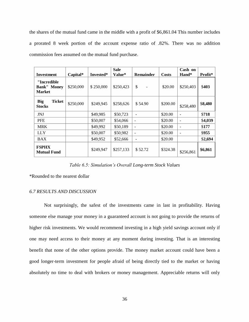
36
the shares of the mutual fund came in the middle with a profit of $6,861.04 This number includes
a prorated 8 week portion of the account expense ratio of .82%. There was no addition
commission fees assumed on the mutual fund purchase.
Investment Capital* Invested*
Sale
Value* Remainder Costs
Cash on
Hand* Profit*
"Incredible
Bank" Money
Market
$250,000 $ 250,000 $250,423 $ - $20.00 $250,403 $403
Big Ticket
Stocks $250,000 $249,945 $258,626 $ 54.90 $200.00
$258,480 $8,480
JNJ $49,985 $50,723 - $20.00 - $718
PFE $50,007 $54,066 - $20.00 - $4,039
MRK $49,992 $50,189 - $20.00 - $177
LLY $50,007 $50,982 - $20.00 - $955
BAX $49,952 $52,666 - $20.00 $2,694
FSPHX
Mutual Fund $249,947 $257,133 $ 52.72 $324.38
$256,861
$6,861
Table 6.5: Simulation’s Overall Long-term Stock Values
*Rounded to the nearest dollar
6.7 RESULTS AND DISCUSSION
Not surprisingly, the safest of the investments came in last in profitability. Having
someone else manage your money in a guaranteed account is not going to provide the returns of
higher risk investments. We would recommend investing in a high yield savings account only if
one may need access to their money at any moment during investing. That is an interesting
benefit that none of the other options provide. The money market account could have been a
good longer-term investment for people afraid of being directly tied to the market or having
absolutely no time to deal with brokers or money management. Appreciable returns will only

37
happen over a long, long time, so over 8 weeks, 1% APY works out to only about .15% return on
the original investment. Not losing money, but not gaining much.
Coming in second was the mutual fund. We chose to tie the entire $250 thousand into one
fund, and allow the fund managers to diversify, although some buyers chose to buy multiple
funds as well. The fund was very erratic in the simulation, and just barely recovered in time to
make a good, $6,861 profit in the end. In a word of caution, this proves the Morningstar ratings
to be very subjective, as we had intentionally picked a fund that was supposedly more stable than
most. With the entire market up, it is possible that the gains were solely due to the buoyancy of
the entire market, and not due to individual success. If the stocks had been sold a few weeks
earlier, the investment in the mutual fund would have lost money. The mutual fund option, while
not perhaps the safest, could fit for someone that wants the potential gains of the market without
the work. The mutual fund realized a full seventeen times the profit of the savings account, and
would have therefore produced a still respectable APY of nearly 18%. Investors must pick their
fund or funds very carefully and consider the large fees that fund managers take on an annual
basis.
In perhaps the biggest surprise of the project, the selection of buying a “Big Ticket
Index” of equal values of stock in five of the largest companies in the healthcare field worked
out very well. Every single stock maintained its original value and after a rough start the stocks
gradually gained valued throughout the simulation. At least in the context of our simulation, the
old time logic of buying “companies you know” proved quiet successful.
The “Big Ticket Index” made a profit of $8,480 overall, with $4,039 of that coming from
the largest individual gainer, Pfizer Incorporated. This profit is the largest of the three long-term
investments. The profit gained by holding our five big ticket stocks for two months yielded over

38
a 22% APY, many times the return from the high yield savings account and 4% APY higher than
the return on the mutual fund. The purchase of the “Big Ticket” stocks was both more consistent
than the mutual fund and the most profitable of the long-term options. Of the three long-term
options we evaluated, it was the best in every measurable way.

39
7. SIMULATION 2: COUNTERTRENDING
In this chapter, we look at the trader strategy countertrending and record its results
throughout the eight-week simulation. Traders using this method can use either technical or
fundamental analysis, but usually go for stocks that are trending and not range-bound.
7.1 WEEK 1 (FEB. 7 – FEB. 12)
This week, trading was started on Tuesday instead of Monday. Stock was bought in
Johnson & Johnson, Abbott Laboratories, Baxter, Biocryst Pharmaceuticals, and CytRx with a
total of six investments made. Johnson & Johnson stock was bought twice, profiting on the first
stock and producing a net loss on the second. Baxter also yielded a net loss, and the other
investments were held on to going into week 2.
On day 1 of week 1 (Feb. 7), 500 shares were bought in Johnson & Johnson at $65.05 a
share for a total of $32,525.00. As Figure 7.1 shows, the company started off the week with stock
selling for over $65.40 and dropped quickly just before Monday closed. Tuesday also started off
low and then when price began increasing, stock was bought. In Figure 7.1, the green mark
signifies the time when the stock was bought, which was at 10:35am, and the red mark represents
when the stock was sold, which was 11:04am at $65.31 for a total of $32,655.00. This yielded a
profit of $120, which includes the $10 trading fees for each transaction. This was very short-
term trading for countertrending that was done on an hourly scale.
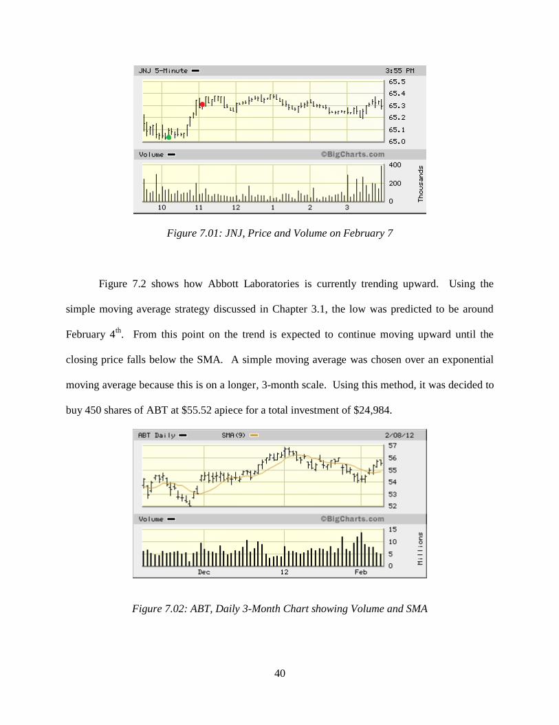
40
Figure 7.01: JNJ, Price and Volume on February 7
Figure 7.2 shows how Abbott Laboratories is currently trending upward. Using the
simple moving average strategy discussed in Chapter 3.1, the low was predicted to be around
February 4th
. From this point on the trend is expected to continue moving upward until the
closing price falls below the SMA. A simple moving average was chosen over an exponential
moving average because this is on a longer, 3-month scale. Using this method, it was decided to
buy 450 shares of ABT at $55.52 apiece for a total investment of $24,984.
Figure 7.02: ABT, Daily 3-Month Chart showing Volume and SMA
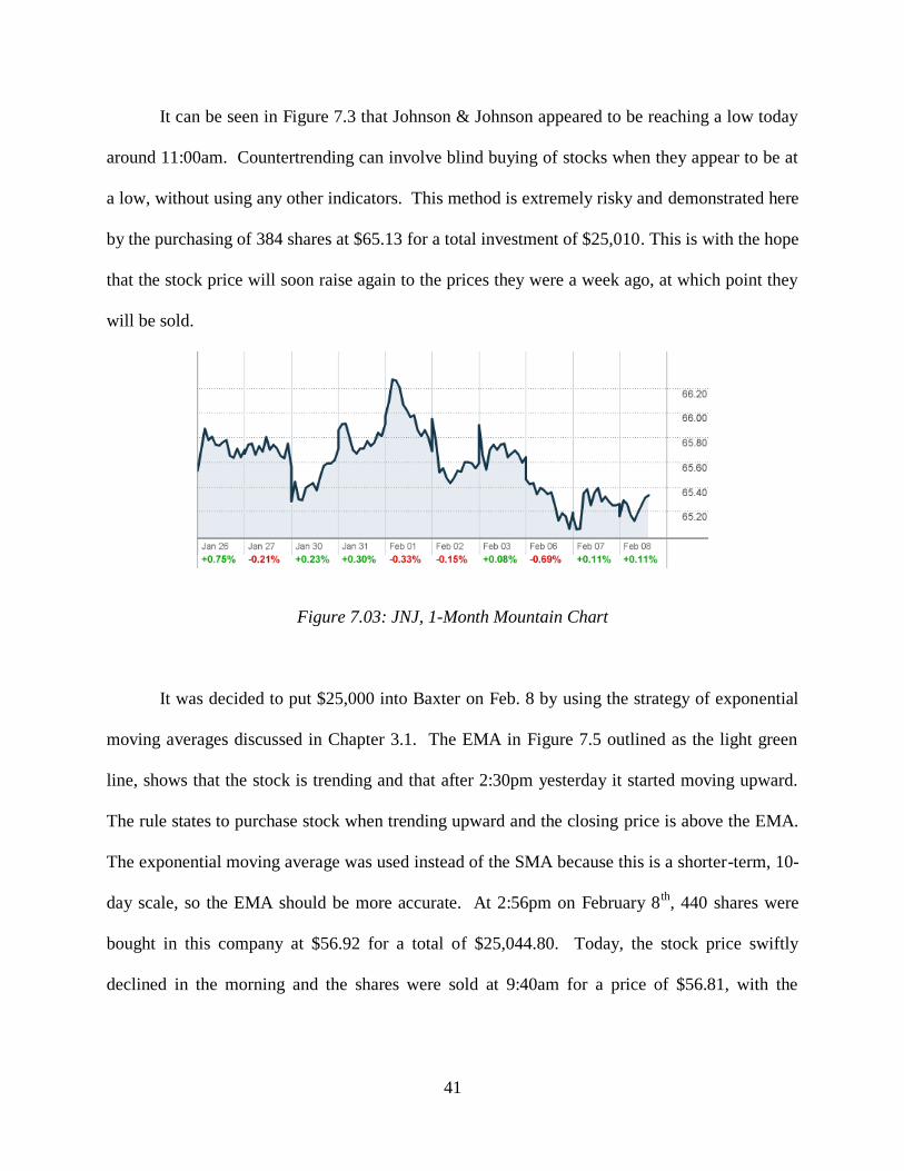
41
It can be seen in Figure 7.3 that Johnson & Johnson appeared to be reaching a low today
around 11:00am. Countertrending can involve blind buying of stocks when they appear to be at
a low, without using any other indicators. This method is extremely risky and demonstrated here
by the purchasing of 384 shares at $65.13 for a total investment of $25,010. This is with the hope
that the stock price will soon raise again to the prices they were a week ago, at which point they
will be sold.
Figure 7.03: JNJ, 1-Month Mountain Chart
It was decided to put $25,000 into Baxter on Feb. 8 by using the strategy of exponential
moving averages discussed in Chapter 3.1. The EMA in Figure 7.5 outlined as the light green
line, shows that the stock is trending and that after 2:30pm yesterday it started moving upward.
The rule states to purchase stock when trending upward and the closing price is above the EMA.
The exponential moving average was used instead of the SMA because this is a shorter-term, 10-
day scale, so the EMA should be more accurate. At 2:56pm on February 8th
, 440 shares were
bought in this company at $56.92 for a total of $25,044.80. Today, the stock price swiftly
declined in the morning and the shares were sold at 9:40am for a price of $56.81, with the

42
intention to cut our losses before price declined further. The overall loss, including the $20 in
transaction fees, was -$64.00.
Figure 7.04: BAX, 10-Day Chart with EMA
Biocryst Pharmaceuticals has been on an uptrend as of mid-December as shown in Figure
7.5. The MACD strategy described in Chapter 3.2 was used to make a trading decision on this
stock. The MACD line just crossed the zero line, indicating direction is to continue with an
uptrend, so 5,100 shares were bought at $3.94 apiece, giving a total invested amount of
$20,094.00. We will be monitoring this stock closely for when the MACD line falls, which will
signal to sell the stock.
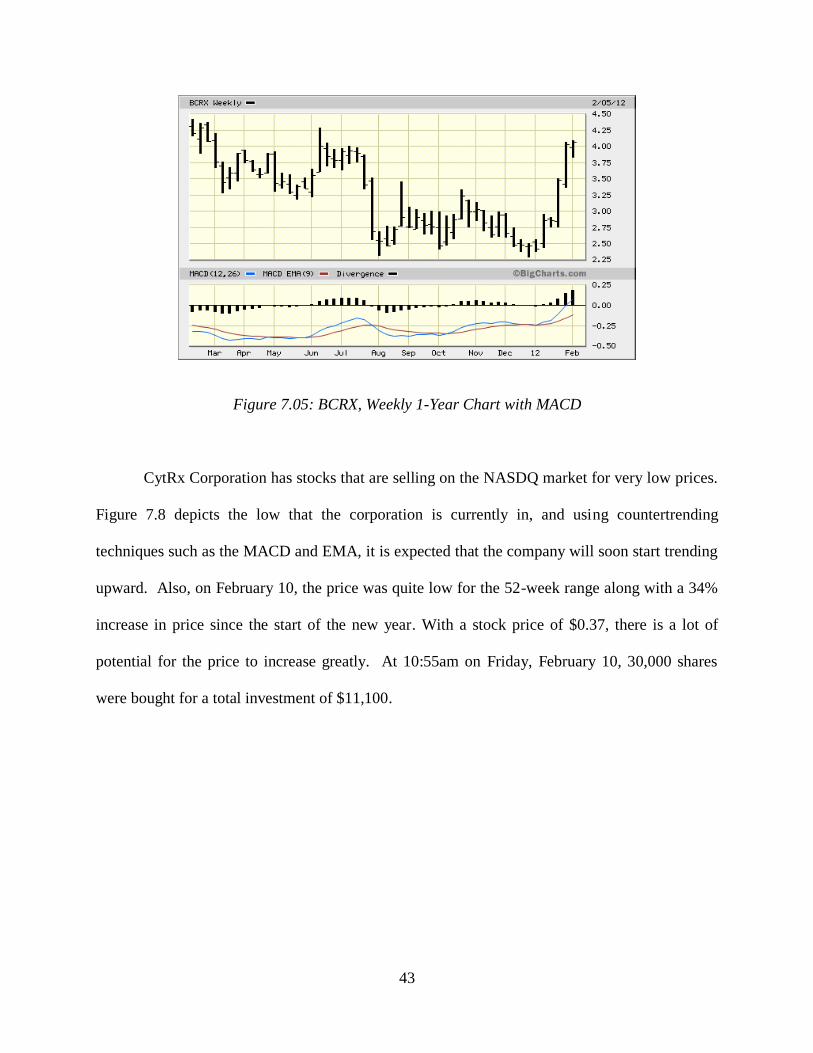
43
Figure 7.05: BCRX, Weekly 1-Year Chart with MACD
CytRx Corporation has stocks that are selling on the NASDQ market for very low prices.
Figure 7.8 depicts the low that the corporation is currently in, and using countertrending
techniques such as the MACD and EMA, it is expected that the company will soon start trending
upward. Also, on February 10, the price was quite low for the 52-week range along with a 34%
increase in price since the start of the new year. With a stock price of $0.37, there is a lot of
potential for the price to increase greatly. At 10:55am on Friday, February 10, 30,000 shares
were bought for a total investment of $11,100.

44
Figure 7.06: CYTR Corporation Weekly 1-Year Chart with MACD
On Wednesday, 384 shares were purchased in Johnson & Johnson at $65.13. This was
because it was blindly guessed that the stock was at a low, and would only increase.
Unfortunately, this method did not work because the stock only increased a little before dropping
again, this time below the original bought price. The downtrend was caught early by the MACD,
which dropped below the signal line and hit the zero line, as shown in Figure 7.7, and all JNJ
stock was sold for a price of $64.64. This gave a net loss of $208.16, but could have been much
worse.
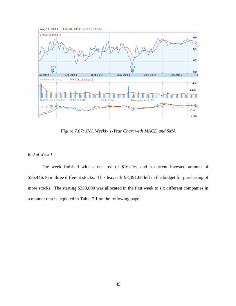
45
Figure 7.07: JNJ, Weekly 1-Year Chart with MACD and SMA
End of Week 1
The week finished with a net loss of $162.16, and a current invested amount of
$56,446.16 in three different stocks. This leaves $193,391.68 left in the budget for purchasing of
more stocks. The starting $250,000 was allocated in the first week to six different companies in
a manner that is depicted in Table 7.1 on the following page.
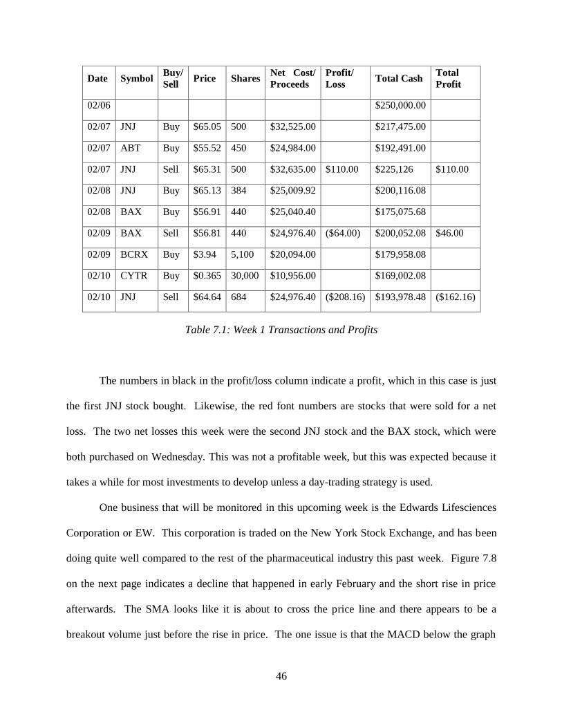
46
Date Symbol Buy/
Sell Price Shares
Net Cost/
Proceeds
Profit/
Loss Total Cash
Total
Profit
02/06 $250,000.00
02/07 JNJ Buy $65.05 500 $32,525.00 $217,475.00
02/07 ABT Buy $55.52 450 $24,984.00 $192,491.00
02/07 JNJ Sell $65.31 500 $32,635.00 $110.00 $225,126 $110.00
02/08 JNJ Buy $65.13 384 $25,009.92 $200,116.08
02/08 BAX Buy $56.91 440 $25,040.40 $175,075.68
02/09 BAX Sell $56.81 440 $24,976.40 ($64.00) $200,052.08 $46.00
02/09 BCRX Buy $3.94 5,100 $20,094.00 $179,958.08
02/10 CYTR Buy $0.365 30,000 $10,956.00 $169,002.08
02/10 JNJ Sell $64.64 684 $24,976.40 ($208.16) $193,978.48 ($162.16)
Table 7.1: Week 1 Transactions and Profits
The numbers in black in the profit/loss column indicate a profit, which in this case is just
the first JNJ stock bought. Likewise, the red font numbers are stocks that were sold for a net
loss. The two net losses this week were the second JNJ stock and the BAX stock, which were
both purchased on Wednesday. This was not a profitable week, but this was expected because it
takes a while for most investments to develop unless a day-trading strategy is used.
One business that will be monitored in this upcoming week is the Edwards Lifesciences
Corporation or EW. This corporation is traded on the New York Stock Exchange, and has been
doing quite well compared to the rest of the pharmaceutical industry this past week. Figure 7.8
on the next page indicates a decline that happened in early February and the short rise in price
afterwards. The SMA looks like it is about to cross the price line and there appears to be a
breakout volume just before the rise in price. The one issue is that the MACD below the graph

47
shows no momentum in favor of an uptrend. For this reason, stock was not bought will be
monitored closely throughout week 2.
Figure 7.08: EW, 1-Year Chart with SMA, Volume, VMA, and MACD
7.2 WEEK 2 (FEB. 13 –FEB. 19)
Total cash coming into this week for the member practicing countertrending trading was
$193,978.48 and the total profit so far had been negative $162.16. Stock was bought in ARAY,
EW, LLY, and XOMA and sold in ARAY, ABT, BCRX, EW, and LLY. No stocks were bought
or sold on Tuesday and on Wednesday, stocks were only sold, none were bought.
It was decided to buy stock in EW at the beginning of the week based on last week’s
data. The 52-week range was low and the MACD implied that an upward momentum swing was
imminent. For these reasons, 350 shares were purchases on day 1 at a price of $74.13, giving a
total investment of $25,945.50.
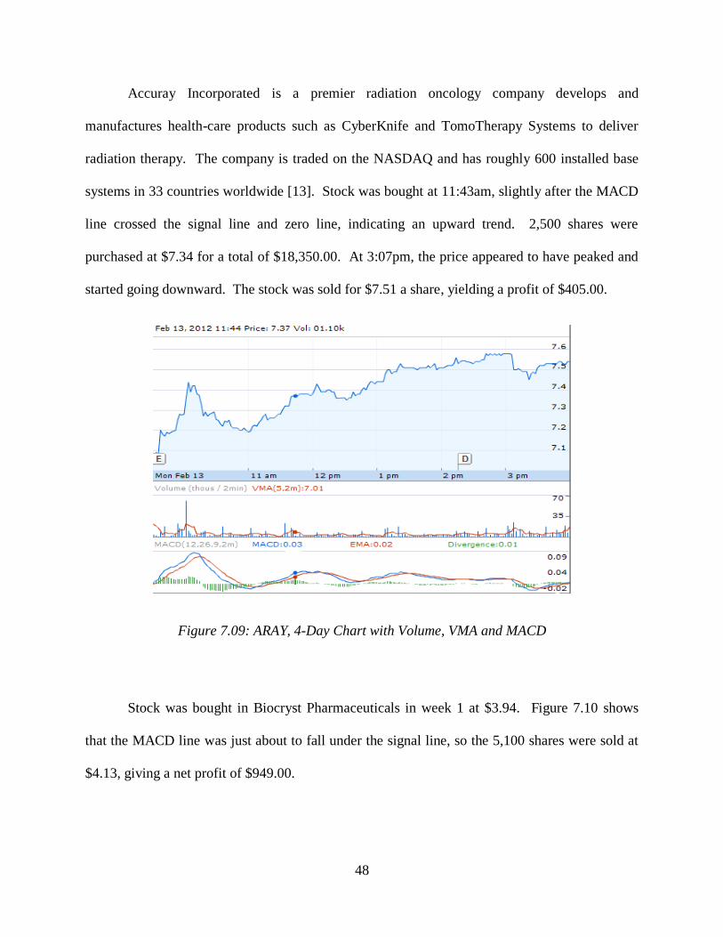
48
Accuray Incorporated is a premier radiation oncology company develops and
manufactures health-care products such as CyberKnife and TomoTherapy Systems to deliver
radiation therapy. The company is traded on the NASDAQ and has roughly 600 installed base
systems in 33 countries worldwide [13]. Stock was bought at 11:43am, slightly after the MACD
line crossed the signal line and zero line, indicating an upward trend. 2,500 shares were
purchased at $7.34 for a total of $18,350.00. At 3:07pm, the price appeared to have peaked and
started going downward. The stock was sold for $7.51 a share, yielding a profit of $405.00.
Figure 7.09: ARAY, 4-Day Chart with Volume, VMA and MACD
Stock was bought in Biocryst Pharmaceuticals in week 1 at $3.94. Figure 7.10 shows
that the MACD line was just about to fall under the signal line, so the 5,100 shares were sold at
$4.13, giving a net profit of $949.00.
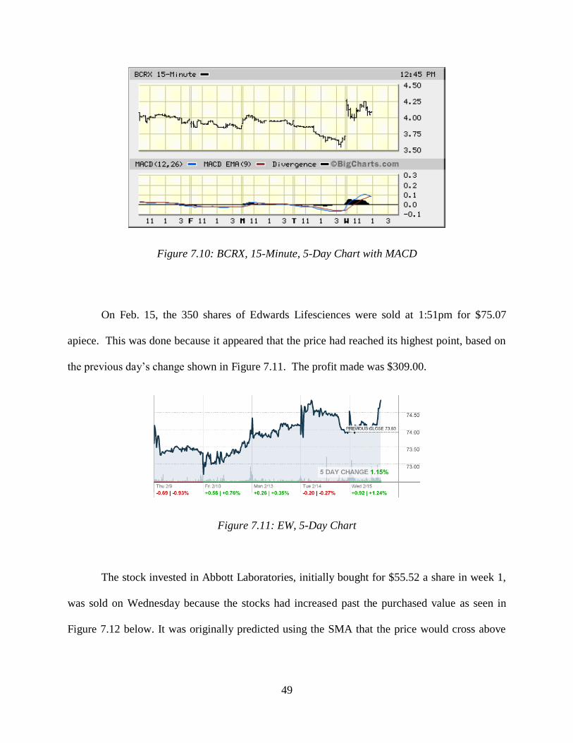
49
Figure 7.10: BCRX, 15-Minute, 5-Day Chart with MACD
On Feb. 15, the 350 shares of Edwards Lifesciences were sold at 1:51pm for $75.07
apiece. This was done because it appeared that the price had reached its highest point, based on
the previous day’s change shown in Figure 7.11. The profit made was $309.00.
Figure 7.11: EW, 5-Day Chart
The stock invested in Abbott Laboratories, initially bought for $55.52 a share in week 1,
was sold on Wednesday because the stocks had increased past the purchased value as seen in
Figure 7.12 below. It was originally predicted using the SMA that the price would cross above
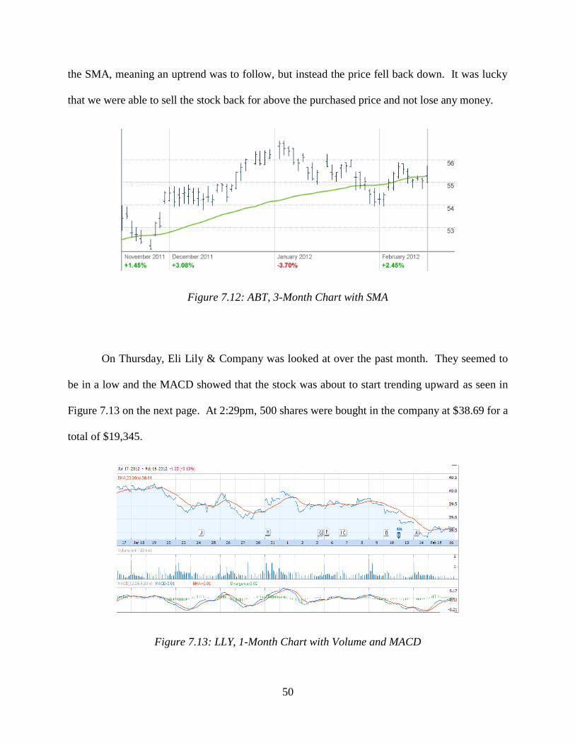
50
the SMA, meaning an uptrend was to follow, but instead the price fell back down. It was lucky
that we were able to sell the stock back for above the purchased price and not lose any money.
Figure 7.12: ABT, 3-Month Chart with SMA
On Thursday, Eli Lily & Company was looked at over the past month. They seemed to
be in a low and the MACD showed that the stock was about to start trending upward as seen in
Figure 7.13 on the next page. At 2:29pm, 500 shares were bought in the company at $38.69 for a
total of $19,345.
Figure 7.13: LLY, 1-Month Chart with Volume and MACD
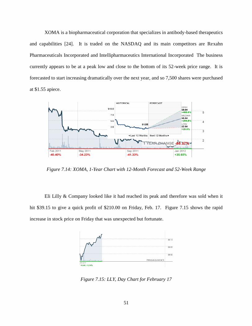
51
XOMA is a biopharmaceutical corporation that specializes in antibody-based therapeutics
and capabilities [24]. It is traded on the NASDAQ and its main competitors are Rexahn
Pharmaceuticals Incorporated and Intellipharmaceutics International Incorporated The business
currently appears to be at a peak low and close to the bottom of its 52-week price range. It is
forecasted to start increasing dramatically over the next year, and so 7,500 shares were purchased
at $1.55 apiece.
Figure 7.14: XOMA, 1-Year Chart with 12-Month Forecast and 52-Week Range
Eli Lilly & Company looked like it had reached its peak and therefore was sold when it
hit $39.15 to give a quick profit of $210.00 on Friday, Feb. 17. Figure 7.15 shows the rapid
increase in stock price on Friday that was unexpected but fortunate.
Figure 7.15: LLY, Day Chart for February 17
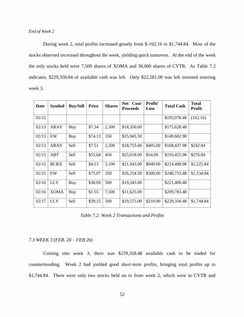
52
End of Week 2
During week 2, total profits increased greatly from $-162.16 to $1,744.84. Most of the
stocks observed increased throughout the week, yielding quick turnovers. At the end of the week
the only stocks held were 7,500 shares of XOMA and 30,000 shares of CYTR. As Table 7.2
indicates, $229,358.84 of available cash was left. Only $22,581.00 was left invested entering
week 3.
Date Symbol Buy/Sell Price Shares Net Cost/
Proceeds
Profit/
Loss Total Cash
Total
Profit
02/12 $193,978.48 (162.16)
02/13 ARAY Buy $7.34 2,500 $18,350.00 $175,628.48
02/13 EW Buy $74.13 350 $25,945.50 $149,682.98
02/13 ARAY Sell $7.51 2,500 $18,755.00 $405.00 $168,437.98 $242.84
02/15 ABT Sell $55.64 450 $25,018.00 $34.00 $193,455.98 $276.84
02/15 BCRX Sell $4.13 5,100 $21,043.00 $949.00 $214,498.98 $1,225.84
02/15 EW Sell $75.07 350 $26,254.50 $309.00 $240,753.48 $1,534.84
02/16 LLY Buy $38.69 500 $19,345.00 $221,408.48
02/16 XOMA Buy $1.55 7,500 $11,625.00 $209,783.48
02/17 LLY Sell $39.15 500 $19,575.00 $210.00 $229,358.48 $1,744.84
Table 7.2: Week 2 Transactions and Profits
7.3 WEEK 3 (FEB. 20 – FEB 26)
Coming into week 3, there was $229,358.48 available cash to be traded for
countertrending. Week 2 had yielded good short-term profits, bringing total profits up to
$1,744.84. There were only two stocks held on to from week 2, which were in CYTR and

53
XOMA. Stock was purchased Monday in IART, and no trading was done on Tuesday, February
21, as the market dropped greatly on this day and stock was bought early on Wednesday in VICL
and DYAX. Again, no stock was traded on Thursday, but on Friday stock was bought late in
JNJ.
On Monday, stock was purchased in Integra Lifesciences Holdings Corporation, which is
traded on the NASDAQ. As seen in Figure 7.16, it appeared that IART was at a low according
to the SMA. The MACD also showed a recent switch, which made us believe an upward trend
was imminent. Volume appeared to be increasing as well, and so 1,000 shares were bought at
$31.41 for a total of $31,410.00.
Figure 7.16: IART, 6-Month Char with SMA, Volume+, and MACD
Also traded on the NASDAQ, Vical Incorporated researches and develops
biopharmaceutical products based on patented DNA delivery technologies. Vical looked like it
was at a low according to Figure 7.17, and had a below-average 52-week range. 5,000 shares

54
were bought at 10:51am when the stock price was $3.31 a share, giving an investment of
$16,550.00.
Figure 7.17: VICL, 3-Month Chart with SMA and MACD
Also bought on Tuesday was stock in another company traded on NASDAQ. Dyax
Corporation has been around since 1989 and is headquartered nearby in Cambridge, MA.
Purchasing 10,000 shares at $1.44 was risky because it was really a guess that DYAX was ready
to turn around from its downtrend as Figure 7.18 displays, but only $14,400.00 was invested and
just the nature of countertrending is risky.
Figure 7.18: DYAX, 3-Month Chart with SMA and MACD

55
Stock was bought in Johnson & Johnson on Friday because there was a huge drop at the
beginning of the day as seen in Figure 7.19. The stock price is also at its lowest point in the past
30 days. Therefor, 935 stocks were bought at a low price of $64.32 for a total investment of over
$60,000.
Figure 7.19: JNJ, 5-Day Chart
Week 3 End:
Week three ended with $106,859.28 of total cash available as seen in Table 7.3. Shares
were purchased in four different companies and no stocks were sold, leaving six stocks that still
have money invested in them. A lot of money was put into Johnson & Johnson because it
appeared to be quite low of a price and is only expected to increase soon.
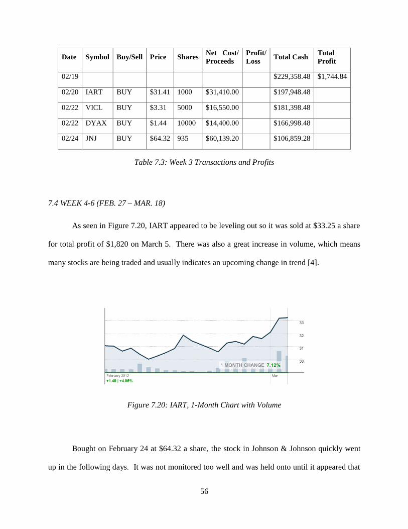
56
Date Symbol Buy/Sell Price Shares Net Cost/
Proceeds
Profit/
Loss Total Cash
Total
Profit
02/19 $229,358.48 $1,744.84
02/20 IART BUY $31.41 1000 $31,410.00 $197,948.48
02/22 VICL BUY $3.31 5000 $16,550.00 $181,398.48
02/22 DYAX BUY $1.44 10000 $14,400.00 $166,998.48
02/24 JNJ BUY $64.32 935 $60,139.20 $106,859.28
Table 7.3: Week 3 Transactions and Profits
7.4 WEEK 4-6 (FEB. 27 – MAR. 18)
As seen in Figure 7.20, IART appeared to be leveling out so it was sold at $33.25 a share
for total profit of $1,820 on March 5. There was also a great increase in volume, which means
many stocks are being traded and usually indicates an upcoming change in trend [4].
Figure 7.20: IART, 1-Month Chart with Volume
Bought on February 24 at $64.32 a share, the stock in Johnson & Johnson quickly went
up in the following days. It was not monitored too well and was held onto until it appeared that
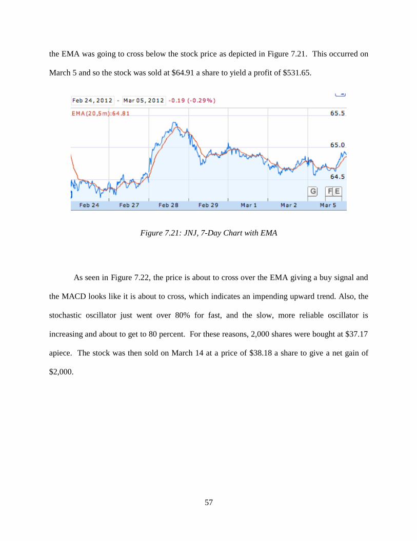
57
the EMA was going to cross below the stock price as depicted in Figure 7.21. This occurred on
March 5 and so the stock was sold at $64.91 a share to yield a profit of $531.65.
Figure 7.21: JNJ, 7-Day Chart with EMA
As seen in Figure 7.22, the price is about to cross over the EMA giving a buy signal and
the MACD looks like it is about to cross, which indicates an impending upward trend. Also, the
stochastic oscillator just went over 80% for fast, and the slow, more reliable oscillator is
increasing and about to get to 80 percent. For these reasons, 2,000 shares were bought at $37.17
apiece. The stock was then sold on March 14 at a price of $38.18 a share to give a net gain of
$2,000.

58
Figure 7.22: MRK, 1-Month Chart with EMA, MACD, and Fast Stochastic
7,500 shares were originally bought in XOMA on February 13 when the stock price was
$1.55 a share. Looking at Figure 7.23, between Wednesday, March 14 and Friday, March 16,
the stock price increased greatly. It was assumed that the price was at its peak and the stock was
sold at $2.30 over the weekend to obtain a profit of $5,605.00.
Figure 7.23: XOMA, 5-Day Chart
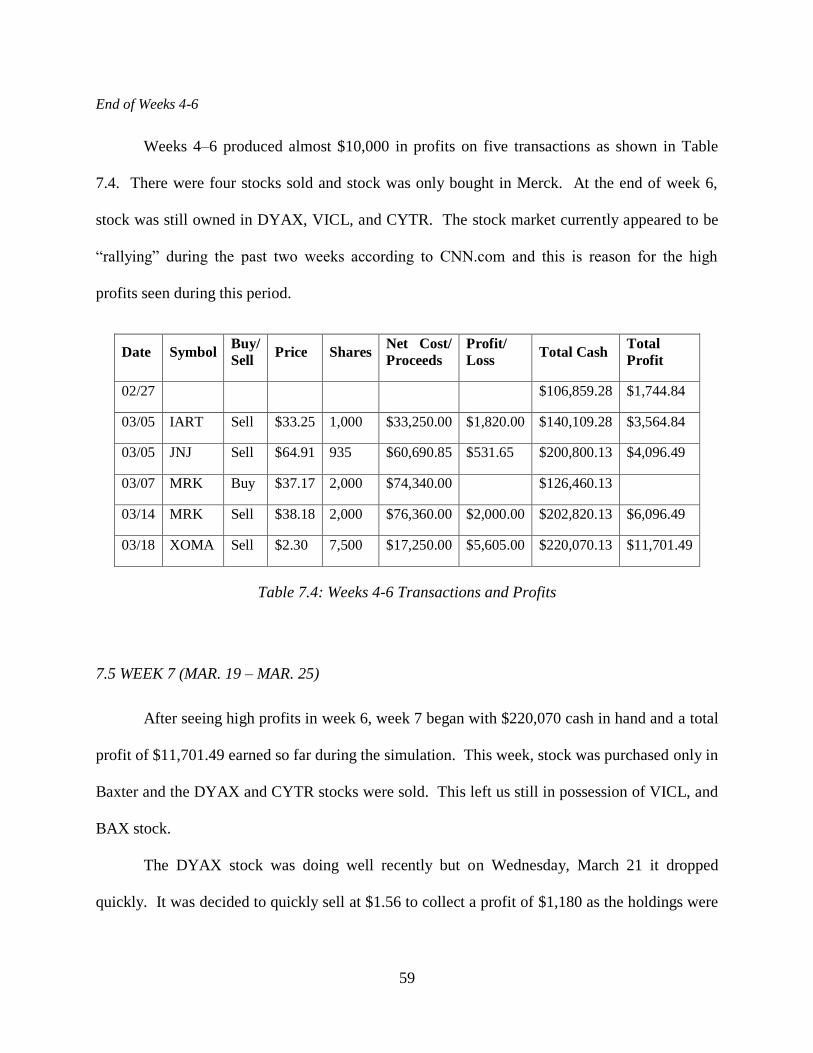
59
End of Weeks 4-6
Weeks 4–6 produced almost $10,000 in profits on five transactions as shown in Table
7.4. There were four stocks sold and stock was only bought in Merck. At the end of week 6,
stock was still owned in DYAX, VICL, and CYTR. The stock market currently appeared to be
“rallying” during the past two weeks according to CNN.com and this is reason for the high
profits seen during this period.
Date Symbol Buy/
Sell Price Shares
Net Cost/
Proceeds
Profit/
Loss Total Cash
Total
Profit
02/27 $106,859.28 $1,744.84
03/05 IART Sell $33.25 1,000 $33,250.00 $1,820.00 $140,109.28 $3,564.84
03/05 JNJ Sell $64.91 935 $60,690.85 $531.65 $200,800.13 $4,096.49
03/07 MRK Buy $37.17 2,000 $74,340.00 $126,460.13
03/14 MRK Sell $38.18 2,000 $76,360.00 $2,000.00 $202,820.13 $6,096.49
03/18 XOMA Sell $2.30 7,500 $17,250.00 $5,605.00 $220,070.13 $11,701.49
Table 7.4: Weeks 4-6 Transactions and Profits
7.5 WEEK 7 (MAR. 19 – MAR. 25)
After seeing high profits in week 6, week 7 began with $220,070 cash in hand and a total
profit of $11,701.49 earned so far during the simulation. This week, stock was purchased only in
Baxter and the DYAX and CYTR stocks were sold. This left us still in possession of VICL, and
BAX stock.
The DYAX stock was doing well recently but on Wednesday, March 21 it dropped
quickly. It was decided to quickly sell at $1.56 to collect a profit of $1,180 as the holdings were
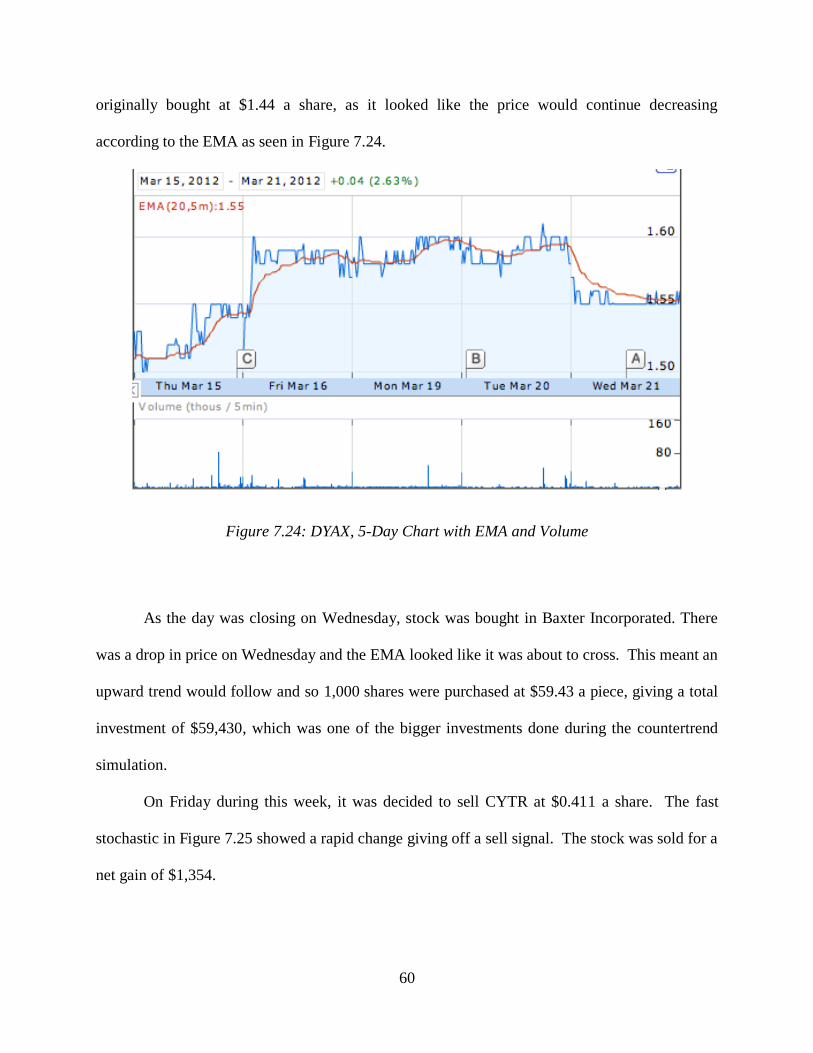
60
originally bought at $1.44 a share, as it looked like the price would continue decreasing
according to the EMA as seen in Figure 7.24.
Figure 7.24: DYAX, 5-Day Chart with EMA and Volume
As the day was closing on Wednesday, stock was bought in Baxter Incorporated. There
was a drop in price on Wednesday and the EMA looked like it was about to cross. This meant an
upward trend would follow and so 1,000 shares were purchased at $59.43 a piece, giving a total
investment of $59,430, which was one of the bigger investments done during the countertrend
simulation.
On Friday during this week, it was decided to sell CYTR at $0.411 a share. The fast
stochastic in Figure 7.25 showed a rapid change giving off a sell signal. The stock was sold for a
net gain of $1,354.

61
Figure 7.25: CYTR, 5-Day Chart with Fast Stochastic
End of Week 7
The end of week 7 brought the total profit up to $14,235.49 as detailed in Table 7.5.
There were only three transactions this week, two of which were selling stock, yielding a net
gain of $2,534 for the week. The only stock bought was 1,000 shares of Baxter, which gave a
total invested amount of $59,000 for the week. The only other stock held onto was VICL at the
end of week 7.
Date Symbol Buy/
Sell Price Shares
Net Cost/
Proceeds
Profit/
Loss Total Cash
Total
Profit
03/18 $220,070.13 $11,701.49
03/21 DYAX Sell $1.56 10,000 $15,580.00 $1,180.00 $235,650.13 $12,881.49
03/21 BAX Buy $59.43 1000 $59,430.00 - $176,220.13 -
03/23 CYTR Sell $0.411 30,000 $12,310.00 $1,354.00 $188,530.13 $14,235.49
Table 7.5: Week 7 Transactions and Profits
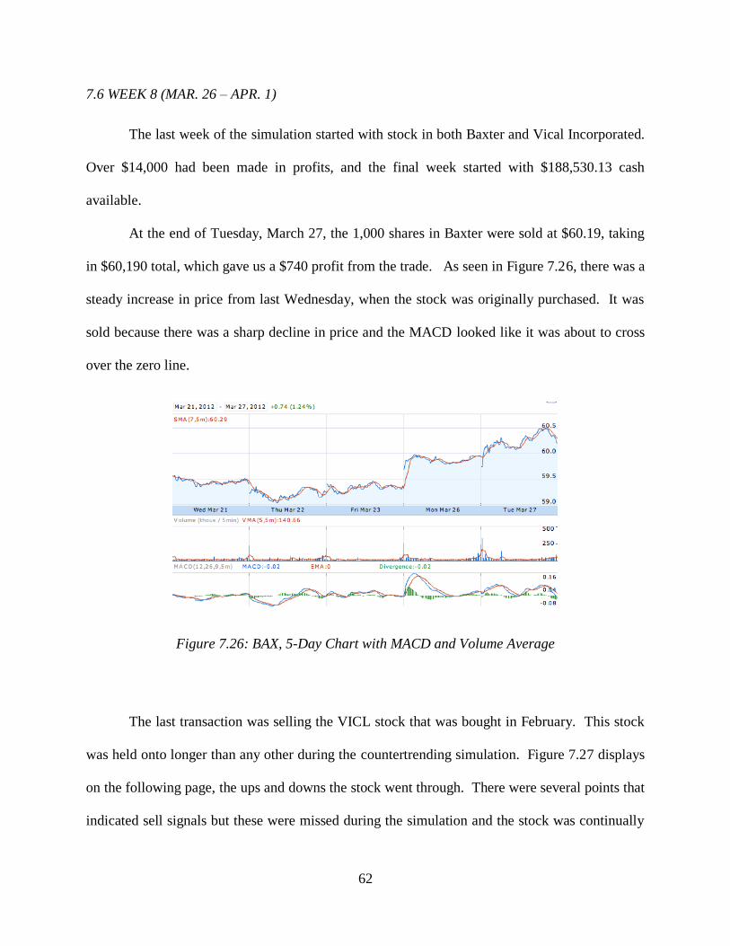
62
7.6 WEEK 8 (MAR. 26 – APR. 1)
The last week of the simulation started with stock in both Baxter and Vical Incorporated.
Over $14,000 had been made in profits, and the final week started with $188,530.13 cash
available.
At the end of Tuesday, March 27, the 1,000 shares in Baxter were sold at $60.19, taking
in $60,190 total, which gave us a $740 profit from the trade. As seen in Figure 7.26, there was a
steady increase in price from last Wednesday, when the stock was originally purchased. It was
sold because there was a sharp decline in price and the MACD looked like it was about to cross
over the zero line.
Figure 7.26: BAX, 5-Day Chart with MACD and Volume Average
The last transaction was selling the VICL stock that was bought in February. This stock
was held onto longer than any other during the countertrending simulation. Figure 7.27 displays
on the following page, the ups and downs the stock went through. There were several points that
indicated sell signals but these were missed during the simulation and the stock was continually
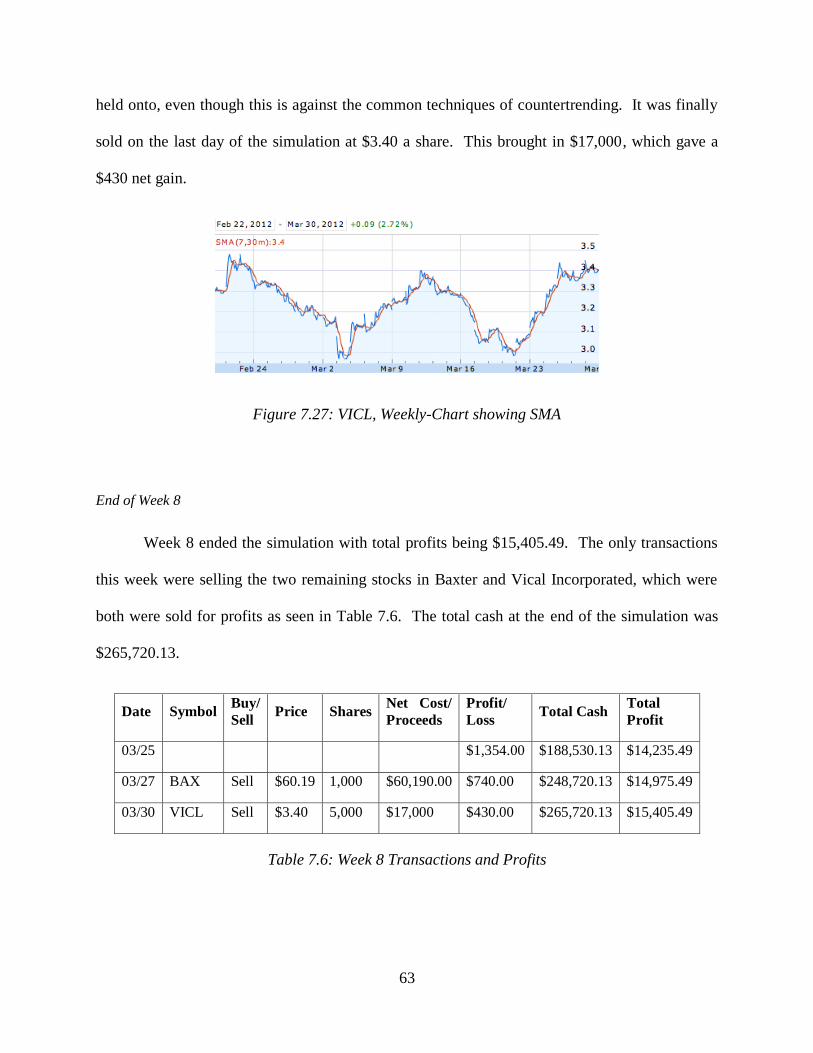
63
held onto, even though this is against the common techniques of countertrending. It was finally
sold on the last day of the simulation at $3.40 a share. This brought in $17,000, which gave a
$430 net gain.
Figure 7.27: VICL, Weekly-Chart showing SMA
End of Week 8
Week 8 ended the simulation with total profits being $15,405.49. The only transactions
this week were selling the two remaining stocks in Baxter and Vical Incorporated, which were
both were sold for profits as seen in Table 7.6. The total cash at the end of the simulation was
$265,720.13.
Date Symbol Buy/
Sell Price Shares
Net Cost/
Proceeds
Profit/
Loss Total Cash
Total
Profit
03/25 $1,354.00 $188,530.13 $14,235.49
03/27 BAX Sell $60.19 1,000 $60,190.00 $740.00 $248,720.13 $14,975.49
03/30 VICL Sell $3.40 5,000 $17,000 $430.00 $265,720.13 $15,405.49
Table 7.6: Week 8 Transactions and Profits

64
7.7 RESULTS AND DISCUSSION
We concluded that the simulation for countertrending was effective because it yielded a
total profit of over $15 thousand. This represents only a little over 6% of the starting cash, and
counter-trending should yield high profits due to great risks. In this simulation though, not many
risks were taken. However, it still produced very acceptable results because a six percent return
on investment over eight weeks translates to an APY of nearly 40%. This is forty times the
interest rate of the highest yielding savings account we could find. We were also timid at first to
put large amounts of money into investments due to our previous lack of knowledge. As the
weeks went on, larger investments were made and higher profits were gained. It was also
difficult to monitor the stock market at all times due to classes and club meetings, causing some
buy or sell signals to be missed. This happened frequently but stocks were almost always held
until they reached their original bought price, which is why there were so few losses using this
method. In a real-life situation, it might be more difficult to hold onto stocks until they turn
around due to personal financial restrictions or if stocks are on a steady decline, which never
really happened during this 8-week period.
Due to the reluctance to invest large amounts of money in the beginning of the
simulation, there was a lag time before total profits became significant. Figure 7.28 on the next
page shows the weekly profits from the simulation in red bars and the total profit as a blue line.
It displays the slow increase in profits from weeks 1–3 and then the exponential increase during
weeks 4–7. The last week had smaller profits because all stocks had to be sold to end the
simulation whether or not it was time to sell these stocks.
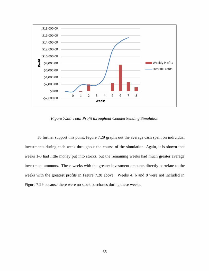
65
Figure 7.28: Total Profit throughout Countertrending Simulation
To further support this point, Figure 7.29 graphs out the average cash spent on individual
investments during each week throughout the course of the simulation. Again, it is shown that
weeks 1-3 had little money put into stocks, but the remaining weeks had much greater average
investment amounts. These weeks with the greater investment amounts directly correlate to the
weeks with the greatest profits in Figure 7.28 above. Weeks 4, 6 and 8 were not included in
Figure 7.29 because there were no stock purchases during these weeks.
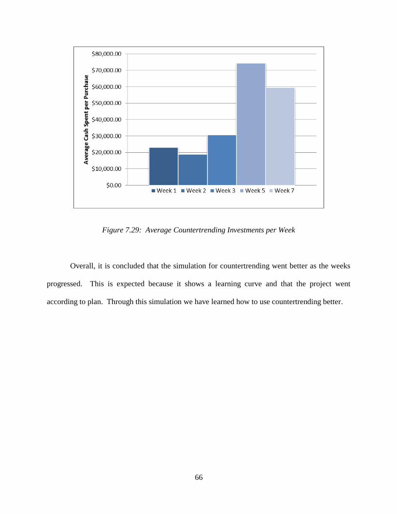
66
Figure 7.29: Average Countertrending Investments per Week
Overall, it is concluded that the simulation for countertrending went better as the weeks
progressed. This is expected because it shows a learning curve and that the project went
according to plan. Through this simulation we have learned how to use countertrending better.

67
8. SIMULATION 3: TREND FOLLOWING
For investment purposes, we have amassed a list of over 500 stocks within the healthcare
industry as a watch list. A program called Wiki Invest was used to sort stocks by many financial
categories to help identify "trenders.” At the same time, during the first week of trading, the
healthcare industry in general performed extremely poorly. Due to the general terrible recent
performance of the market, we recompiled the list of tickers by potential investments 1 day
gains, showing a few positive numbers at the top. Once ordered, the 52-week price range of the
stock and the 1 year chart of prices were used to narrow down potential trending stocks. If a
stock has a low price, it is more likely to draw investment attention due to increased cost basis
potential if gains occur. Only select stocks met these criteria. Longer-term stock charts (such as
5yr) were used to generalize the possibility for continued growth or the possible over valuation
of the stock price. Final candidates were selected by showing a positive EMA 100 curve with
good long-term potential. News and outside information are generally disregarded in favor of
following pure data trends.
8.1 WEEK 1 (FEB. 7 – FEB.12)
In the first week, small investments were made in trending stocks. Stocks were identified
to be trending if the price was increasing for at least several weeks, and EMA and other market
derivative tools were used to confirm investment targets. Total cash coming into this week for
the member practicing trend following trading was $250,000. Stock was bought in UGLX, KUN,
WLP, JAZZ, DXCM, ARAY. No stocks were sold.
Urologix is a leader in products to treat Benign Prostatic Hyperplasia. The possible
purchase of this stock was triggered by a positive weekly gain, putting it to the top of the first

68
filter in Wiki Invest. Figure 8.1 showed a promising growth over time and the longer-term charts
showed no deal breaking current overbalance. The price was at the low end of its 52-week range,
and very affordable for a stock listed on NASDAQ (pulling in only $1.27 at the time of
purchase). A final check of the one year chart shown below confirms a well-established upward
trend, shown more clearly in brown as an EMA 100 curve. The trend is present, and the stock
met all other criteria, save being slightly risky at a market cap of only roughly $23 million, so the
purchase was ordered. For the uniform trade fee of ten dollars, 2,000 shares of UGLX were
purchased at $1.27 at 10:55am. These will be held until a large reversal in the one year trend
occurs, and then dumped to maximize the profit from trending before reversal.
Figure 8.01: UGLX, 1-Year Chart with EMA and Volume
China Shenghuo Pharmaceutical Holdings Incorporated is a company that combines
eastern traditional medicine with modern science for Asian markets [12]. The stock initially

69
caught in the filter for having a positive week gain. The low price overall in both its 52-week
range and as a value drew special attention, similar to why we purchased UGLX later.
The one-year stock price chart seen as Figure 8.2, with EMA 100 shows a trend clearly
establishing in the second half of January into February. Using a longer-term chart and the fact
that the stock was at one of its lowest recent prices, this trend could be quite profitable, because a
small dollar amount increase per share price would lead to extremely large cost benefit per share.
Again it is a riskier, smaller stock, but the profits if the trend continues outweigh those concerns.
On Tuesday at 9:40 am, 4,000 shares were purchased in KUN, at a price of $0.54. These will be
held until a reversal in the established upwards trend occurs, then dumped to maximize the profit
from trending before reversal. We invested because we expect this company to post small gains
for a long period.
Figure 8.02: KUN, 1-Year Chart with EMA and Volume
Forest Laboratories is a pharmaceutical company that makes both generic and brand
name prescription pharmaceuticals, in an attempt to diversify to larger stocks with higher market

70
capitalizations than UGLX and KUN. Forest Laboratories currently has a market capitalization
of $8.42 billion. The stock price is currently lower in its 52-week range, and in general the prices
travels on longer range projections between the high twenties and forty dollars per share. It has a
low price to earnings ratio, which is roughly half of the healthcare industry average so the stock
is currently undervalued by that metric.
The 1 year stock price chart in Figure 8.3 is a little less clear than in the case of UGLX or
KUN, but it clearly shows a general uptick of the EMA 100 curve, despite recent daily losses. If
the price continues to trend, even within its 52-week high, there is substantial profit to be made.
The stock price is currently near the bottom of a long slide, so there is a high chance of a long
resurgence. On Wednesday, at 9:38AM, we purchased 158 shares of FXR, at $31.63. We will
sell only if the trend reverses for at least 15 days or so.
Figure 8.03: FXR, 1-Year Chart with EMA and Volume
Jazz Pharmaceuticals make specialty drugs for unaddressed market areas. The stock is at
the top of very long upward trend. This extremely established trend shows no signs of reversing.
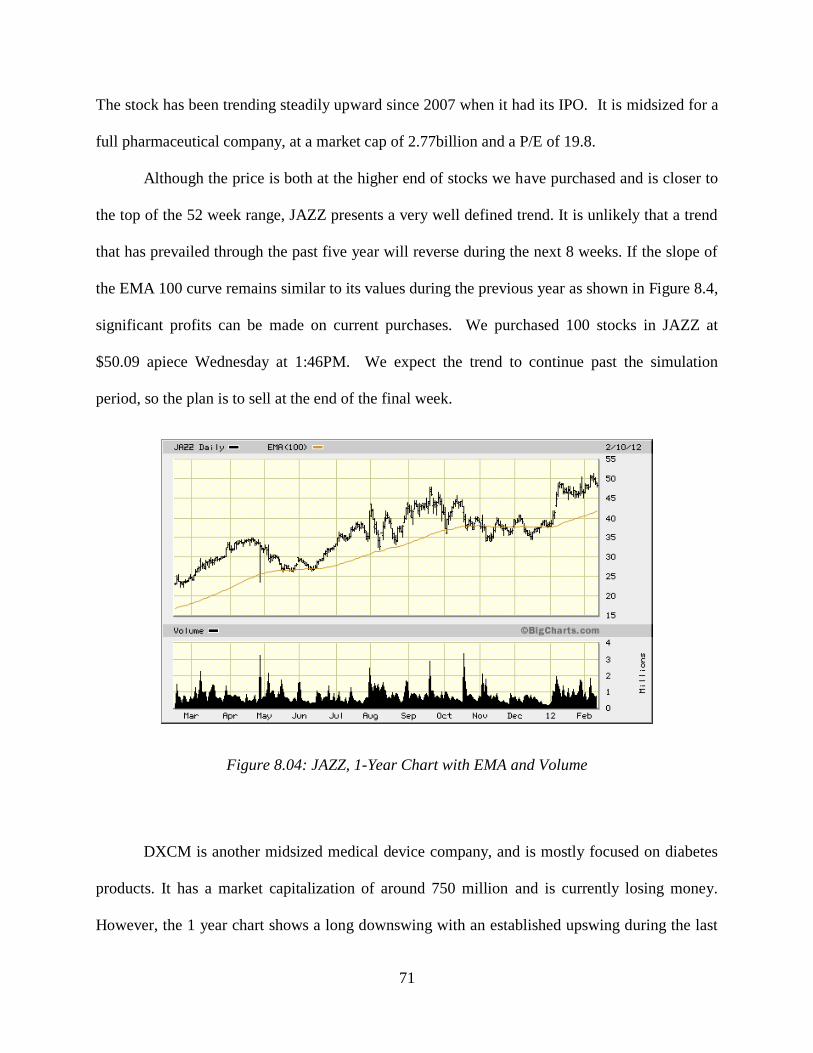
71
The stock has been trending steadily upward since 2007 when it had its IPO. It is midsized for a
full pharmaceutical company, at a market cap of 2.77billion and a P/E of 19.8.
Although the price is both at the higher end of stocks we have purchased and is closer to
the top of the 52 week range, JAZZ presents a very well defined trend. It is unlikely that a trend
that has prevailed through the past five year will reverse during the next 8 weeks. If the slope of
the EMA 100 curve remains similar to its values during the previous year as shown in Figure 8.4,
significant profits can be made on current purchases. We purchased 100 stocks in JAZZ at
$50.09 apiece Wednesday at 1:46PM. We expect the trend to continue past the simulation
period, so the plan is to sell at the end of the final week.
Figure 8.04: JAZZ, 1-Year Chart with EMA and Volume
DXCM is another midsized medical device company, and is mostly focused on diabetes
products. It has a market capitalization of around 750 million and is currently losing money.
However, the 1 year chart shows a long downswing with an established upswing during the last

72
month or so of the EMA (100). If the price recovers to its 52 week high, a profit from the current
price of 11.12 could be as high as 5 dollars a share. Its longer-term prospects show a potential for
growth or at least the return of higher stock prices.
Although from a news standpoint, the company is currently reporting a negative P/E
ratio, the positive showing of the 1 year EMA in Figure 8.5, and a strong rumor of takeover by a
larger company made this an appealing stock. On Thursday at 10:39AM, we purchased 200
shares of DXCM at $11.16 apiece. We expect a long-term recovery to occur, and do not plan to
sell if small single day or week downturns occur.
Figure 8.05: DXCM, 1-Year Chart with EMA and Volume
WellPoint is one of the largest health insurance providers in the nation, and owns the
more locally based Anthem Blue Cross Blue Shield. They represent a very large, mostly stable
large cap stock, it an attempt to decrease the overall risk and increase the stability of the trend

73
following portfolio. WLP features the longest and least steep trend of all of the stocks purchased,
but was one of the few market giants not in a current downtrend.
If this stock continues the trend shown by the EMA 500 curve in the five year stock price
chart in Figure 8.6, and recovers anywhere near the 2007 high, gains could reach as high as about
$30 per share over time. The trend has been established since the market crash with the housing
bubble, so it is a relatively safe trend that could yield modest returns in a short period such as
eight weeks. On Friday at 11:50AM we purchased 79 shares of WellPoint Health Network for
$64.02 apiece.
Figure 8.06: WLP, 5-Year Chart with EMA and Volume
Research after the closing bell on Friday revealed the ideal positioning of Accuray or
ARAY. ARAY has a market capitalization of around half a billion dollars, and a negative P/E
ratio. The company draws its growth from manufacturing equipment for cancer surgeries and the
removal of solid tumors.
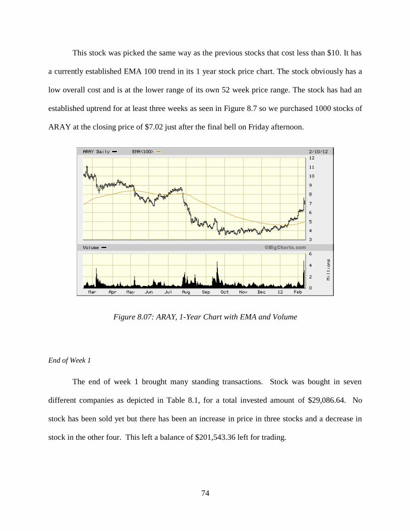
74
This stock was picked the same way as the previous stocks that cost less than $10. It has
a currently established EMA 100 trend in its 1 year stock price chart. The stock obviously has a
low overall cost and is at the lower range of its own 52 week price range. The stock has had an
established uptrend for at least three weeks as seen in Figure 8.7 so we purchased 1000 stocks of
ARAY at the closing price of $7.02 just after the final bell on Friday afternoon.
Figure 8.07: ARAY, 1-Year Chart with EMA and Volume
End of Week 1
The end of week 1 brought many standing transactions. Stock was bought in seven
different companies as depicted in Table 8.1, for a total invested amount of $29,086.64. No
stock has been sold yet but there has been an increase in price in three stocks and a decrease in
stock in the other four. This left a balance of $201,543.36 left for trading.
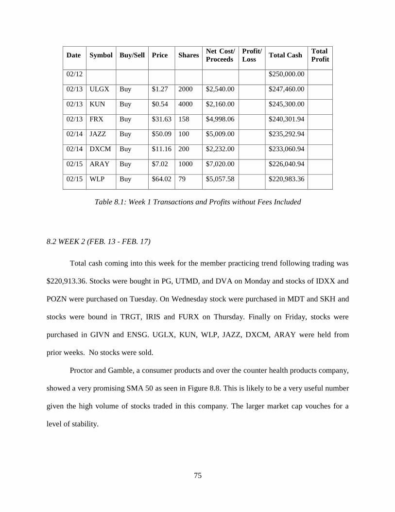
75
Date Symbol Buy/Sell Price Shares Net Cost/
Proceeds
Profit/
Loss Total Cash
Total
Profit
02/12 $250,000.00
02/13 ULGX Buy $1.27 2000 $2,540.00 $247,460.00
02/13 KUN Buy $0.54 4000 $2,160.00 $245,300.00
02/13 FRX Buy $31.63 158 $4,998.06 $240,301.94
02/14 JAZZ Buy $50.09 100 $5,009.00 $235,292.94
02/14 DXCM Buy $11.16 200 $2,232.00 $233,060.94
02/15 ARAY Buy $7.02 1000 $7,020.00 $226,040.94
02/15 WLP Buy $64.02 79 $5,057.58 $220,983.36
Table 8.1: Week 1 Transactions and Profits without Fees Included
8.2 WEEK 2 (FEB. 13 - FEB. 17)
Total cash coming into this week for the member practicing trend following trading was
$220,913.36. Stocks were bought in PG, UTMD, and DVA on Monday and stocks of IDXX and
POZN were purchased on Tuesday. On Wednesday stock were purchased in MDT and SKH and
stocks were bound in TRGT, IRIS and FURX on Thursday. Finally on Friday, stocks were
purchased in GIVN and ENSG. UGLX, KUN, WLP, JAZZ, DXCM, ARAY were held from
prior weeks. No stocks were sold.
Proctor and Gamble, a consumer products and over the counter health products company,
showed a very promising SMA 50 as seen in Figure 8.8. This is likely to be a very useful number
given the high volume of stocks traded in this company. The larger market cap vouches for a
level of stability.
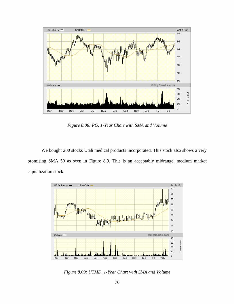
76
Figure 8.08: PG, 1-Year Chart with SMA and Volume
We bought 200 stocks Utah medical products incorporated. This stock also shows a very
promising SMA 50 as seen in Figure 8.9. This is an acceptably midrange, medium market
capitalization stock.
Figure 8.09: UTMD, 1-Year Chart with SMA and Volume

77
We bought 250 stocks in DVA or DA Vita incorporated. This is a high stock price per
unit, but shows again a very promising upward trend in the SMA 50 in Figure 8.10, which shows
the previous 52 weeks. The stock earned $505 in increased value its first week.
Figure 8.10: DVA, 1-Year Chart with SMA and Volume
We bought 100 shares in IDEXX Laboratories. It is another high priced high cap stock
that showed a very promising upward trend in the SMA 50 according to Figure 8.11. It should
yield high, relatively low risk profits if the trend continues.

78
Figure 8.11: IDEXX, 1-Year Chart with SMA and Volume
We also bought on Tuesday 3,000 stocks of POZN or Pozen pharmaceuticals as it is more
widely known. This is a very high number of individuals stocks, but the low stock price and the
very promising upward trend in the SMA 50 shown in Figure 8.12 pushed us to do it. A small
dollar increased would produce thousands in profits over upcoming weeks.
Figure 8.12: POZN, 1-Year Chart with SMA and Volume
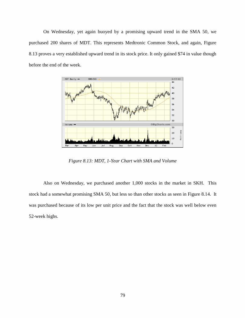
79
On Wednesday, yet again buoyed by a promising upward trend in the SMA 50, we
purchased 200 shares of MDT. This represents Medtronic Common Stock, and again, Figure
8.13 proves a very established upward trend in its stock price. It only gained $74 in value though
before the end of the week.
Figure 8.13: MDT, 1-Year Chart with SMA and Volume
Also on Wednesday, we purchased another 1,000 stocks in the market in SKH. This
stock had a somewhat promising SMA 50, but less so than other stocks as seen in Figure 8.14. It
was purchased because of its low per unit price and the fact that the stock was well below even
52-week highs.
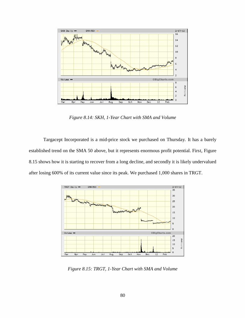
80
Figure 8.14: SKH, 1-Year Chart with SMA and Volume
Targacept Incorporated is a mid-price stock we purchased on Thursday. It has a barely
established trend on the SMA 50 above, but it represents enormous profit potential. First, Figure
8.15 shows how it is starting to recover from a long decline, and secondly it is likely undervalued
after losing 600% of its current value since its peak. We purchased 1,000 shares in TRGT.
Figure 8.15: TRGT, 1-Year Chart with SMA and Volume

81
IRIS International shows a decently established upward trend in the SMA 50 curve in
Figure 8.16 below. It has already in fact surpassed its 52-week high, but there is more profit to be
made, as we believe the trend will continue. We purchased a total of 1,000 IRIS stocks on
Thursday, and they gained $320 in total value by Friday closing bell.
Figure 8.16: IRIS, 1-Year Chart with SMA and Volume
FURX or Furiex Pharmaceuticals is a drug development company based in the United
States. The SMA in Figure 8.17 shows it has already leveled off slightly, but it has slightly
continued on its three to four month upward trend. It is a very small for a listed company so
could show quite large percentage growth numbers if the market treats it well.

82
Figure 8.17: FURX, 1-Year Chart with SMA and Volume
GIVN is the first stock we purchased on the final day of trading for the second week. In
Figure 8.18, the SMA 50 line shows it is an established upward trender, and although it lost $45
during the rest of the day on Friday, so large returns were expected. The price is still several
dollars below the stock's 52-week high. We purchased 250 stocks in Given Imaging.
Figure 8.18: GIVN, 1-Year Chart with SMA and Volume

83
The final stock purchased using trend following this week was ENSG or the Ensign
Group which provides nursing and rehab services. We purchased this stock because although the
SMA 50 curve in Figure 8.19 did not show a large slop or heavy dollar gains, it did show a very
consistent and established trend in the market. We purchased 200 stocks in the Ensign group.
Figure 8.19: ENSG, 1-Year Chart with SMA and Volume
End of Week 2
We made a running gain off new investments of $2,576.50 and the running gain of old
investments from prior weeks of was $1,093.55, for a total portfolio value increase of $3,669.55.
No profit was made because no stocks were sold as seen in Table 8.2. None of the trends that
stocks were purchased on have reversed, as the period of one week was too short to know
definitively. We have spent a total of $133,535.64 on investment and fees, leaving $116,464.36
in cash on hand for future transactions.

84
Date Symbol Buy/Sell Price Shares Net Cost/
Proceeds
Profit/
Loss Total Cash
Total
Profit
02/12 $220,913.36
02/13 PG Buy $64.34 150 $9,651.00 $211,262.36
02/13 UTMD Buy $29.57 200 $5,914.00 $205,348.36
02/13 DVA Buy $83.70 250 $20,925.00 $184,423.36
02/14 IDXX Buy $86.98 100 $8,698.00 $175,725.36
02/14 POZN Buy $4.32 3000 $12,960.00 $162,765.36
02/15 MDT Buy $39.57 200 $7,914.00 $154,851.36
02/15 SKH Buy $6.75 1000 $6,750.00 $148,101.36
02/16 TRGT Buy $6.68 1000 $6,690.00 $141,411.36
02/16 IRIS Buy $11.22 1000 $11,220.00 $130,191.36
02/16 FURX Buy $16.91 200 $3,382.00 $126,809.36
02/17 GIVN Buy $18.94 250 $4,735.00 $122,074.36
02/17 ENSG Buy $27.50 200 $5,500.00 $116,574.36
Table 8.2: Week 2 Transactions and Profits without Fees Included
8.3 WEEK 3 (FEB. 20 – FEB 26)
Coming into the week, the group member practicing trend following had $116,464.36 in
cash on hand for trading. Monday was a bank holiday, and was not a market day, so therefore no
trading took place. No stocks were purchased on Tuesday. On Wednesday, stock was purchased
in ISRG, and in DEPO. On Thursday, stocks were purchased in UNH and GNSZ. No stocks
were purchased on Friday.
Again for the third consecutive week no stocks were sold. In fact, the trend following
simulation has yet to sell any stocks. It is important to remember though, that counter trend stock
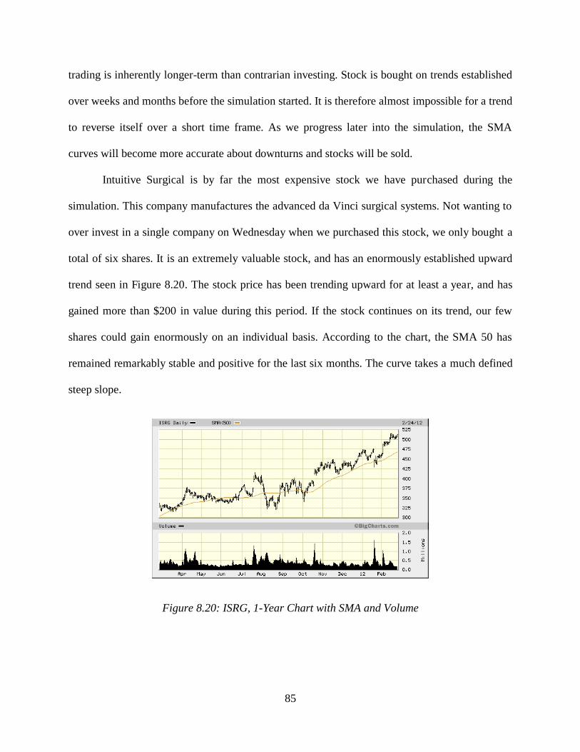
85
trading is inherently longer-term than contrarian investing. Stock is bought on trends established
over weeks and months before the simulation started. It is therefore almost impossible for a trend
to reverse itself over a short time frame. As we progress later into the simulation, the SMA
curves will become more accurate about downturns and stocks will be sold.
Intuitive Surgical is by far the most expensive stock we have purchased during the
simulation. This company manufactures the advanced da Vinci surgical systems. Not wanting to
over invest in a single company on Wednesday when we purchased this stock, we only bought a
total of six shares. It is an extremely valuable stock, and has an enormously established upward
trend seen in Figure 8.20. The stock price has been trending upward for at least a year, and has
gained more than $200 in value during this period. If the stock continues on its trend, our few
shares could gain enormously on an individual basis. According to the chart, the SMA 50 has
remained remarkably stable and positive for the last six months. The curve takes a much defined
steep slope.
Figure 8.20: ISRG, 1-Year Chart with SMA and Volume

86
Depomed Incorporated is the company behind the acronym, and the company
manufactures drugs that use its various oral delivery patents. DEPO stock has shown a nice
growth percentage wise over the last several months. The stock is traveling on an established
trend upward, and has been according to the SMA 50 curve for at least two months as shown in
Figure 8.21. The stock price overall is low, and it was therefore possible to buy quite a few
shares of DEPO. We purchased a full 1,000 shares of DEPO. This cost only $6,450 and was
worthy due to the decent curve and the high, penny stock type potential for growth.
Figure 8.21: DEPO, 1-Year Chart with SMA and Volume
UNH stands for United Healthcare Group, a company that operates by offering health
benefit plans to individual consumers and to businesses. It has a very large market capitalization,
currently over fifty billion dollars, and the general stability of being a NYSE listed company.
The stock is very close to the high end of its 52-week range, which could speak negatively about
its expected growth. However the SMA 50 line in Figure 8.22 shows a clear, steady and positive
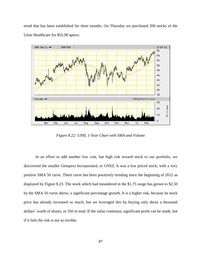
87
trend that has been established for three months. On Thursday we purchased 200 stocks of the
Unite Healthcare for $55.98 apiece.
Figure 8.22: UNH, 1-Year Chart with SMA and Volume
In an effort to add another low cost, but high risk reward stock to our portfolio, we
discovered the smaller Genspera Incorporated, or GNSZ. It was a low priced stock, with a very
positive SMA 50 curve. There curve has been positively trending since the beginning of 2012 as
displayed by Figure 8.23. The stock which had meandered in the $1.75 range has grown to $2.50
by the SMA 50 curve above, a significant percentage growth. It is a higher risk, because its stock
price has already increased so much, but we leveraged this by buying only about a thousand
dollars’ worth of shares, or 350 in total. If the value continues, significant profit can be made, but
if it fails the risk is not so terrible.

88
Figure 8.23: GNSZ, 1-Year Chart with SMA and Volume
End of Week 3
This week, a total of $21,722 was spent on new investments and fees. The stocks
purchased consisted of ISRG. DEPO, UNH, GNSZ. All investments from prior weeks were held,
and no additional stock was purchased in those companies. The total profit of the trend following
remains zero, since no stocks were sold. The total gain in value of the new portion of the
portfolio was $290.56, and the gain in value of the old holdings compared to purchase price was
$3,737.37. This gives us a total value gained in the portfolio of $4,027.93. The total cash on hand
after the week's trading finished was $94,732.36. Table 8.3 on the following page shows the
complete week’s transactions.

89
Date Symbol Buy/Sell Price Shares Net Cost/
Proceeds
Profit/
Loss Total Cash
Total
Profit
$116,464.36
02/12 ISRG Buy $503.50 6 $3,021.00 $113,433.36
02/13 DEPO Buy $6.45 1000 $6,450.00 $106,973.36
02/13 UNH Buy $55.98 200 $11,196.00 $95,767.36
02/13 GNSZ Buy $2.90 350 $1,015.00 $94,742.36
Table 8.3: Week 3 Transactions and Profits
8.4 WEEKS 4-6 (FEB. 27 –MAR.18)
Coming into week 4, the group member practicing trend following had $94,732.36 in
cash on hand for trading. No trading occurred Monday, Wednesday, or Thursday. On Tuesday,
stock was purchased in AGN, IART, and AFFY. On Friday stocks were purchased in TEAR and
VAR. All previously held shares of KUN were also sold on Friday. Trading, reflecting that the
simulation is nearly half over, and switched from looking at 1 year trends to two month trends.
At the beginning of week 5, the trader held $33,799.36 in cash. On Monday, stock was
purchase in LLY, and on Thursday stock was purchased in CYNO. No stocks were sold in week
5. At the beginning of week 6, the trader had $25,196.36 in cash on hand. No stocks were bought
or sold in week six.
All three stocks, AGN, IART, and AFFY wtih charts displayed above were purchased on
Tuesday Febuary 28th. All of the stocks were purchased becuase their SMA 25 lines show a
trend in their two month stock price charts. In all, these stocks have a chance to be a longer-term
investment than day trading but produce quicker short-term profits than stocks bought on 1year
SMA 50 trends. The investments totatal $8,753 in AGN, $15,860 in IART and $10,510 in AFFY

90
VAR stock was and is expensive, but shows a nice uptick in its SMA curve in Figure
8.24. This curve shows its progress up to the end of week 6. This stock has a trend, but a shorter
trend that will hopefully earn more money in the short four weeks remaining in the simulation.
On Friday, March 2nd we purchased 300 shares of VAR at $65.20 apiece.
Figure 8.24: VAR, 2-Month Chart with SMA and Volume
KUN stock was sold because it shows a clear turn in its SMA 50 in Figure 8.25. The
trend has clearly been reversed and money is being lost, so it was time to sell. This stock was
sold for a final profit of $180, including buy and sell commissions. It clearly did not meet our
original trend expectations.
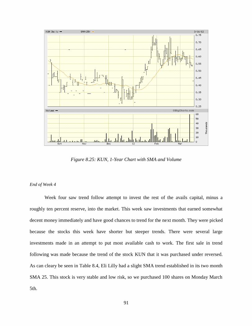
91
Figure 8.25: KUN, 1-Year Chart with SMA and Volume
End of Week 4
Week four saw trend follow attempt to invest the rest of the avails capital, minus a
roughly ten percent reserve, into the market. This week saw investments that earned somewhat
decent money immediately and have good chances to trend for the next month. They were picked
because the stocks this week have shorter but steeper trends. There were several large
investments made in an attempt to put most available cash to work. The first sale in trend
following was made because the trend of the stock KUN that it was purchased under reversed.
As can cleary be seen in Table 8.4, Eli Lilly had a slight SMA trend established in its two month
SMA 25. This stock is very stable and low risk, so we purchased 100 shares on Monday March
5th.
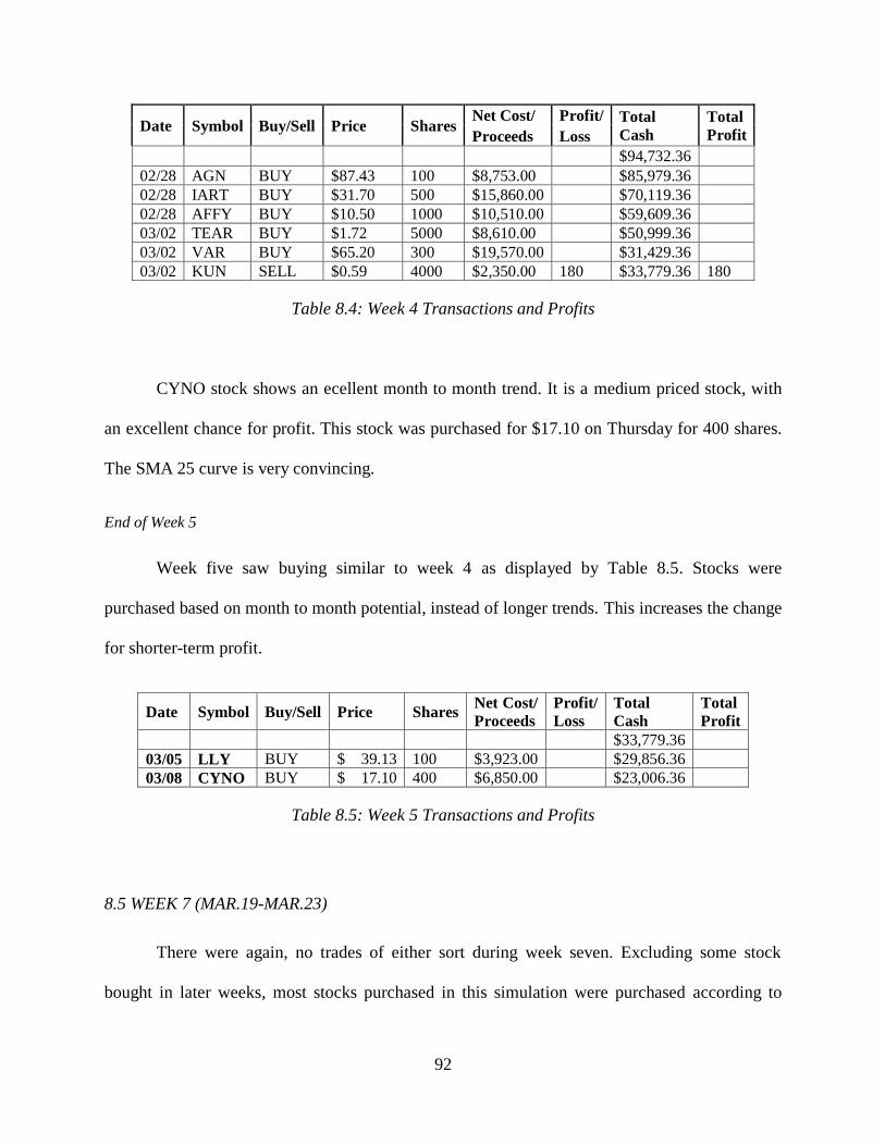
92
Date Symbol Buy/Sell Price Shares Net Cost/ Profit/ Total
Cash
Total
Profit Proceeds Loss
$94,732.36
02/28 AGN BUY $87.43 100 $8,753.00
$85,979.36
02/28 IART BUY $31.70 500 $15,860.00
$70,119.36
02/28 AFFY BUY $10.50 1000 $10,510.00
$59,609.36
03/02 TEAR BUY $1.72 5000 $8,610.00
$50,999.36
03/02 VAR BUY $65.20 300 $19,570.00
$31,429.36
03/02 KUN SELL $0.59 4000 $2,350.00 180 $33,779.36 180
Table 8.4: Week 4 Transactions and Profits
CYNO stock shows an ecellent month to month trend. It is a medium priced stock, with
an excellent chance for profit. This stock was purchased for $17.10 on Thursday for 400 shares.
The SMA 25 curve is very convincing.
End of Week 5
Week five saw buying similar to week 4 as displayed by Table 8.5. Stocks were
purchased based on month to month potential, instead of longer trends. This increases the change
for shorter-term profit.
Date Symbol Buy/Sell Price Shares Net Cost/
Proceeds
Profit/
Loss
Total
Cash
Total
Profit
$33,779.36
03/05 LLY BUY $ 39.13 100 $3,923.00
$29,856.36
03/08 CYNO BUY $ 17.10 400 $6,850.00
$23,006.36
Table 8.5: Week 5 Transactions and Profits
8.5 WEEK 7 (MAR.19-MAR.23)
There were again, no trades of either sort during week seven. Excluding some stock
bought in later weeks, most stocks purchased in this simulation were purchased according to

93
stable one year trends. According to the trend following methods, it is too late in the game to
purchase any more new stocks. There is just not enough time to realize any substantial gains on a
new stock over a week or two, at least not off an established trend. Several stocks however are
on a short-term watch list to sell early next week.
There first of these stocks, one of the larger month long-term investments purchased
during week 4, has gained nearly double its value already. Its trend has not yet reversed, but is
primed to do so. This stock will be sold very quickly. Other stocks on the block to be sold early
in the week include Da Vita, UNH, and TRGT.
End of Week 7
The stocks performed well during the prior week. The largest gainer, both in dollars and
as a percentage was TEAR, which has nearly gained an additional 100% of its original value.
Other stocks also had gains, although stocks picked on longer-terms performed less adequately
during the trading week. The total gained value of stocks in the account currently stands at
$22,733.26. This would be an excellent profit, and should only grow before the mass selloff at
the closing of the final week of the simulation. Trend following, as a whole, is proving a
successful method of investing.
8.6 WEEK 8 (MAR.26-MAR.30)
This was the last week of simulation, so with the longer-term nature of Trend Following,
no stocks were purchase during the trading week. On Tuesday, stock was sold in TEAR. This
stock was purchased on a step but more volatile month long trend, so to maximize the “meat in
the middle” profit, it need to be sold as so as its stock curve dipped into a negative slope, because
value could be lost just as quickly as it was gained. It lost value every day of the final week of

94
trading, so it was the correct decision to sell on Tuesday. The actual information that provoked
the sale was poor performance at the end of the prior week and on Monday of the eighth week.
On Tuesday at 10:10 AM, 5,000 shares of TEAR were sold for a return of $3.77 per share. This
represented a shocking 219% of the original sum invested.
End of Week 8
The stocks performed decently well during the prior week. As the main theme of this
section of the simulation, the trend following method allowed for little action in the short eight
weeks. Only two of the stocks reversed trends enough to be sold. It was said in some of our
research that trend followers can expect to sometimes lose up to 40% of their initial investment
on longer-term trends, before the stock recovers. This project had no shortage of stock that lost
money. There was also however, many stocks that made money. As part of the closing
simulation, all currently held stocks were sold, with a ten dollar commission at the closing price
on Friday March 30th
. This was done to allow maximum time for trends to continue. It is likely
the majority of stocks would have been held for much longer had the simulation continued. An
overall loss was taken on the sales of JAZZ, DXCM, MDT, TRGT, GIVN, ENSG, and DEPO.
The trends that these stocks were purchase on either failed to continue, or were too erratic for
short-term gains. The largest single loss came on TRGT, which lost $1,580, and the rest of the
losing stocks lost less than $215 each.
The rest of the stocks earned value, and produced a profit after trading fees were
removed. The largest three gainers were TEAR, POZN, and IRIS, earning profits of $10
thousand, $5 thousand, $2.2 thousand respectively. The other nineteenth gainers earned an
average of $609.09 apiece. The entire transaction log, and the running losses and profits can be
seen in Table 8.6 on the next page.
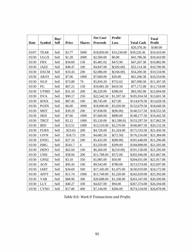
95
Date Symbol
Buy/
Sell Price Shares
Net Cost/ Profit/
Total Cash
Total
Profit Proceeds Loss
$20,376.36 $180.00
03/07 TEAR Sell $3.77 5000 $18,850.00 $10,230.00 $39,226.36 $10,410.00
03/30 ULGX Sell $1.28 2000 $2,560.00 $0.00 $41,786.36 $10,410.00
03/30 FRX Sell $34.69 158 $5,481.02 $472.96 $47,267.38 $10,882.96
03/30 JAZZ Sell $48.47 100 $4,847.00 $(182.00) $52,114.38 $10,700.96
03/30 DXCM Sell $10.43 200 $2,086.00 $(166.00) $54,200.38 $10,534.96
03/30 ARAY Sell $7.06 1000 $7,060.00 $20.00 $61,260.38 $10,554.96
03/30 WLP Sell $73.80 79 $5,830.20 $752.62 $67,090.58 $11,307.58
03/30 PG Sell $67.21 150 $10,081.50 $410.50 $77,172.08 $11,718.08
03/30 UTMD Sell $31.10 200 $6,220.00 $286.00 $83,392.08 $12,004.08
03/30 DVA Sell $90.17 250 $22,542.50 $1,597.50 $105,934.58 $13,601.58
03/30 IDXX Sell $87.45 100 $8,745.00 $27.00 $114,679.58 $13,628.58
03/30 POZN Sell $6.00 3000 $18,000.00 $5,020.00 $132,679.58 $18,648.58
03/30 MDT Sell $39.19 200 $7,838.00 $(96.00) $140,517.58 $18,552.58
03/30 SKH Sell $7.66 1000 $7,660.00 $890.00 $148,177.58 $19,442.58
03/30 TRGT Sell $5.12 1000 $5,120.00 $(1,580.0) $153,297.58 $17,862.58
03/30 IRIS Sell $13.51 1000 $13,510.00 $2,270.00 $166,807.58 $20,132.58
03/30 FURX Sell $23.63 200 $4,726.00 $1,324.00 $171,533.58 $21,456.58
03/30 GIVN Sell $18.73 250 $4,682.50 $(72.50) $176,216.08 $21,384.08
03/30 ENSG Sell $27.16 200 $5,432.00 $(88.00) $181,648.08 $21,296.08
03/30 ISRG Sell $541.7 6 $3,250.00 $209.00 $184,898.08 $21,505.08
03/30 DEPO Sell $62.60 100 $6,260.00 $(210.00) $191,158.08 $21,295.08
03/30 UNH Sell $58.94 200 $11,788.00 $572.00 $202,946.08 $21,867.08
03/30 GNSZ Sell $3.10 350 $1,085.00 $50.00 $204,031.08 $21,917.08
03/30 AGN Sell $95.43 100 $9,543.00 $780.00 $213,574.08 $22,697.08
03/30 IART Sell $34.69 500 $17,345.00 $1,475.00 $230,919.08 $24,172.08
03/30 AFFY Sell $11.74 1000 $11,740.00 $1,220.00 $242,659.08 $25,392.08
03/30 VAR Sell $68.96 300 $20,688.00 $1,108.00 $263,347.08 $26,500.08
03/30 LLY Sell $40.27 100 $4,027.00 $94.00 $267,374.08 $26,594.08
03/30 CYNO Sell $17.86 400 $7,144.00 $284.00 $274,518.08 $26,878.08
Table 8.6: Week 8 Transactions and Profits
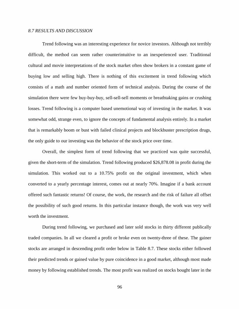
96
8.7 RESULTS AND DISCUSSION
Trend following was an interesting experience for novice investors. Although not terribly
difficult, the method can seem rather counterintuitive to an inexperienced user. Traditional
cultural and movie interpretations of the stock market often show brokers in a constant game of
buying low and selling high. There is nothing of this excitement in trend following which
consists of a math and number oriented form of technical analysis. During the course of the
simulation there were few buy-buy-buy, sell-sell-sell moments or breathtaking gains or crushing
losses. Trend following is a computer based unemotional way of investing in the market. It was
somewhat odd, strange even, to ignore the concepts of fundamental analysis entirely. In a market
that is remarkably boom or bust with failed clinical projects and blockbuster prescription drugs,
the only guide to our investing was the behavior of the stock price over time.
Overall, the simplest form of trend following that we practiced was quite successful,
given the short-term of the simulation. Trend following produced $26,878.08 in profit during the
simulation. This worked out to a 10.75% profit on the original investment, which when
converted to a yearly percentage interest, comes out at nearly 70%. Imagine if a bank account
offered such fantastic returns! Of course, the work, the research and the risk of failure all offset
the possibility of such good returns. In this particular instance though, the work was very well
worth the investment.
During trend following, we purchased and later sold stocks in thirty different publically
traded companies. In all we cleared a profit or broke even on twenty-three of these. The gainer
stocks are arranged in descending profit order below in Table 8.7. These stocks either followed
their predicted trends or gained value by pure coincidence in a good market, although most made
money by following established trends. The most profit was realized on stocks bought later in the
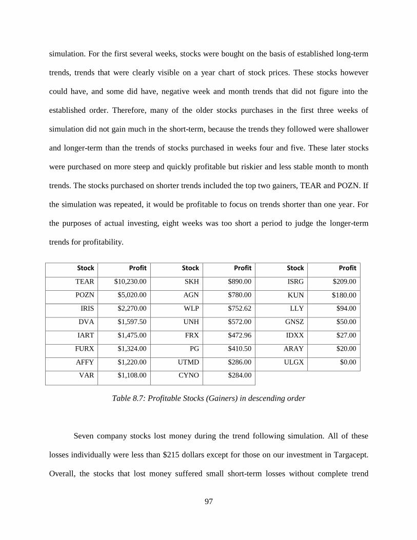
97
simulation. For the first several weeks, stocks were bought on the basis of established long-term
trends, trends that were clearly visible on a year chart of stock prices. These stocks however
could have, and some did have, negative week and month trends that did not figure into the
established order. Therefore, many of the older stocks purchases in the first three weeks of
simulation did not gain much in the short-term, because the trends they followed were shallower
and longer-term than the trends of stocks purchased in weeks four and five. These later stocks
were purchased on more steep and quickly profitable but riskier and less stable month to month
trends. The stocks purchased on shorter trends included the top two gainers, TEAR and POZN. If
the simulation was repeated, it would be profitable to focus on trends shorter than one year. For
the purposes of actual investing, eight weeks was too short a period to judge the longer-term
trends for profitability.
Stock Profit Stock Profit Stock Profit
TEAR $10,230.00 SKH $890.00 ISRG $209.00
POZN $5,020.00 AGN $780.00 KUN $180.00
IRIS $2,270.00 WLP $752.62 LLY $94.00
DVA $1,597.50 UNH $572.00 GNSZ $50.00
IART $1,475.00 FRX $472.96 IDXX $27.00
FURX $1,324.00 PG $410.50 ARAY $20.00
AFFY $1,220.00 UTMD $286.00 ULGX $0.00
VAR $1,108.00 CYNO $284.00
Table 8.7: Profitable Stocks (Gainers) in descending order
Seven company stocks lost money during the trend following simulation. All of these
losses individually were less than $215 dollars except for those on our investment in Targacept.
Overall, the stocks that lost money suffered small short-term losses without complete trend

98
reversal. If they had suffered complete trend reversal, the stocks would have been sold earlier in
the simulation instead of held to the end. The stocks merely lost some value on short-term
tribulations and may have returned to profitability in a longer-term simulation. We believe our
initial predictions for many of these stocks could still prove true over time. Targacept is the
exception to this optimism however. In our original explanation of the purchase, we wrote that
“It has a barely established trend on the SMA 50 above, but it represents enormous profit
potential”. This erroneous prediction proved far too optimistic. We did not wait long enough for
a trend to sufficiently establish, and therefore fell into the biggest pitfall of trend following.
Every other stock was purchased on at least a moderately well-established trend, whereas this
stock was purchased on some gains over two weeks and the belief that it was undervalued.
Perhaps one of the best testaments to the trend following method is the fact that our largest loss
occurred on a stock in which the purchase strayed from our baselines. Had we not bent the rules,
perhaps the loss on TRGT stock, a loss of over five times greater than the next largest setback
would have never occurred. The list of losing stocks, in order of largest to least loss, is presented
in Table 8.8 below.
Stock Loss
TRGT $1,580.00
DEPO $210.00
JAZZ $182.00
DXCM $166.00
MDT $96.00
ENSG $88.00
GIVN $72.50
Table 8.8: Negative Earning Stocks (losers) in Descending Order
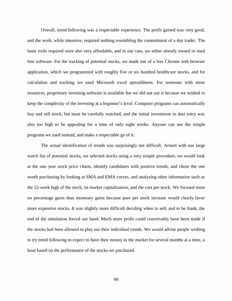
99
Overall, trend following was a respectable experience. The profit gained was very good,
and the work, while intensive, required nothing resembling the commitment of a day trader. The
basic tools required were also very affordable, and in our case, we either already owned or used
free software. For the tracking of potential stocks, we made use of a free Chrome web browser
application, which we programmed with roughly five or six hundred healthcare stocks, and for
calculation and tracking we used Microsoft excel spreadsheets. For someone with more
resources, proprietary investing software is available but we did not use it because we wished to
keep the complexity of the investing at a beginner’s level. Computer programs can automatically
buy and sell stock, but must be carefully watched, and the initial investment in data entry was
also too high to be appealing for a time of only eight weeks. Anyone can use the simple
programs we used instead, and make a respectable go of it.
The actual identification of trends was surprisingly not difficult. Armed with our large
watch list of potential stocks, we selected stocks using a very simple procedure; we would look
at the one year stock price charts, identify candidates with positive trends, and chose the one
worth purchasing by looking at SMA and EMA curves, and analyzing other information such as
the 52-week high of the stock, its market capitalization, and the cost per stock. We focused more
on percentage gains than monetary gains because pure per stock increase would clearly favor
more expensive stocks. It was slightly more difficult deciding when to sell, and to be frank, the
end of the simulation forced our hand. Much more profit could conceivably have been made if
the stocks had been allowed to play out their individual trends. We would advise people wishing
to try trend following to expect to have their money in the market for several months at a time, a
least based on the performance of the stocks we purchased.
100
Finally, similar to what would be expected from a novice, hesitancy on our part cost
some potential profit. We had never invested heavily into the market before, and we originally
invested slowly. We took a few weeks to get the majority of the money invested, and over
$100,000 of capital was not invested until the project was nearly halfway through. This certainly
represents a significant hurdle in a two month simulation, and we believe that in a longer-term
simulation or one conducted by a now more experienced investor would have profited more and
sooner. To not have all of the money in the market as soon as possible was a great inefficiency,
and the only aspect of the trend following simulation we would change greatly in the future. The
caution was not unwarranted as is shown by the large Targacept losses on an incorrectly
identified trend. More money could have been lost than earned if we rushed into trading. On a
final note we would also possibly make less, perhaps better investments in the future, as the
larger more considered investments tended to produce better returns. Table 8.9 below shows the
profitability of the three largest total investments by percent and the three smallest.
Size Stock Sale Price Profit Percentage Profit in % of Sale price
30th GNSZ $1,085.00 $50.00 5%
29th DXCM $2,086.00 ($166.00) -8%
28th ULGX $2,560.00 $0.00 0%
3rd TEAR $18,850.00 $10,230.00 54%
2nd VAR $20,688.00 $1,108.00 5%
1st DVA $22,542.50 $1,597.50 7%
Table 8.9: Profitability of Largest Investments Compared with Smallest Investments
The smaller, less well conceived investments made much less money, even as the very
small sample of the project shows. In the future we would make fewer, more researched
purchases for larger dollar amounts, while maintaining enough diversity to weather incorrect

101
predictions. For $250,000, or the original capital in the project, we would perhaps choose ten or
fifteen companies instead of 30.
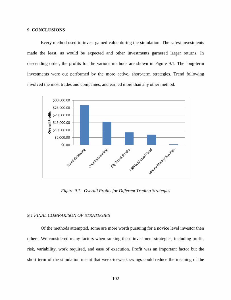
102
9. CONCLUSIONS
Every method used to invest gained value during the simulation. The safest investments
made the least, as would be expected and other investments garnered larger returns. In
descending order, the profits for the various methods are shown in Figure 9.1. The long-term
investments were out performed by the more active, short-term strategies. Trend following
involved the most trades and companies, and earned more than any other method.
Figure 9.1: Overall Profits for Different Trading Strategies
9.1 FINAL COMPARISON OF STRATEGIES
Of the methods attempted, some are more worth pursuing for a novice level investor then
others. We considered many factors when ranking these investment strategies, including profit,
risk, variability, work required, and ease of execution. Profit was an important factor but the
short term of the simulation meant that week-to-week swings could reduce the meaning of the
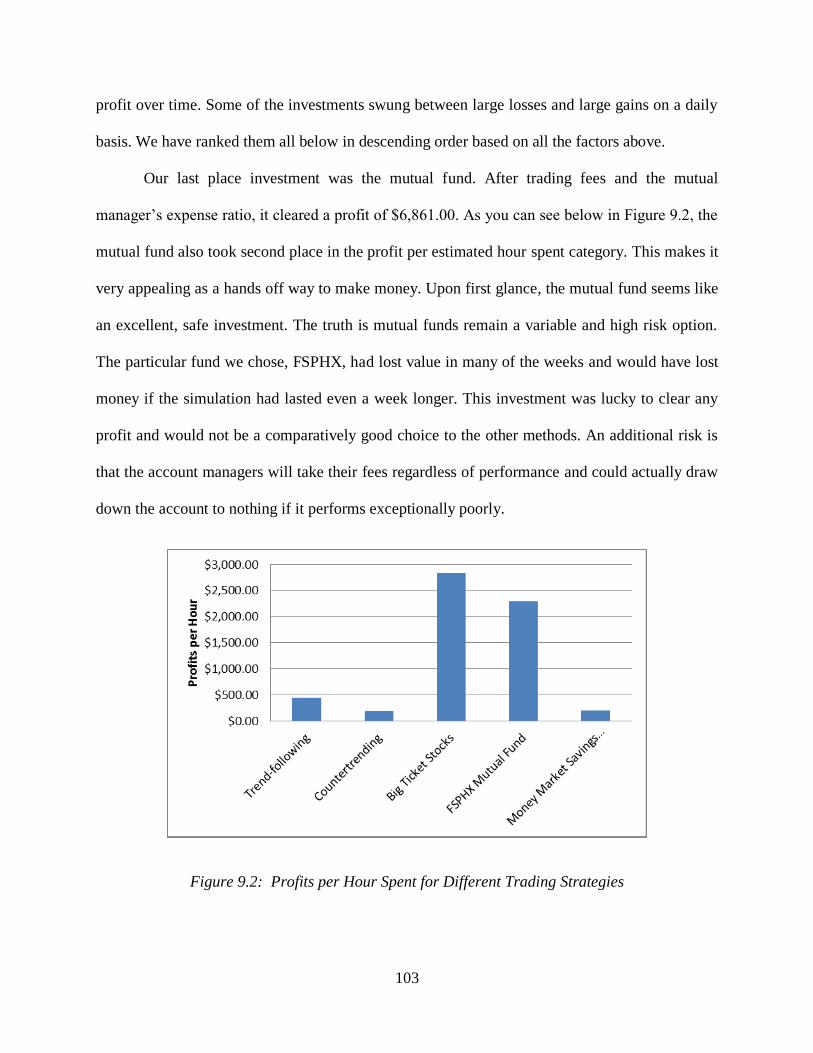
103
profit over time. Some of the investments swung between large losses and large gains on a daily
basis. We have ranked them all below in descending order based on all the factors above.
Our last place investment was the mutual fund. After trading fees and the mutual
manager’s expense ratio, it cleared a profit of $6,861.00. As you can see below in Figure 9.2, the
mutual fund also took second place in the profit per estimated hour spent category. This makes it
very appealing as a hands off way to make money. Upon first glance, the mutual fund seems like
an excellent, safe investment. The truth is mutual funds remain a variable and high risk option.
The particular fund we chose, FSPHX, had lost value in many of the weeks and would have lost
money if the simulation had lasted even a week longer. This investment was lucky to clear any
profit and would not be a comparatively good choice to the other methods. An additional risk is
that the account managers will take their fees regardless of performance and could actually draw
down the account to nothing if it performs exceptionally poorly.
Figure 9.2: Profits per Hour Spent for Different Trading Strategies
104
The money market savings account came in second place among the investments studied.
It is a good option for people wishing simply to preserve their money for later. The return of
about $400 is certainly unimpressive for $250,000 in capital. The savings account actually came
in last place in both total profit and second to last in profit per hour spent. The return is so low
that the initial time spent to setup the account garners less than the other investments, even
though no other labor was required. The account is actually likely to lose money over a long
period because national inflation rates generally hover between pits of about 2% and peaks of
roughly 15% [25]. It is very safe place to invest but is unlikely to garner any substantial profits.
The lack of variability, the safety, and the ability to access or remove the money at any time
without penalty gives this the edge over investing in a mutual fund.
Big Ticket Index was an interesting experience. Buying stock in companies “you know”
proved to be quite profitable. The stocks were bought with the thought that stable companies
with established customer bases tend to gain value over time. While this assertation certainly is
not always true, the investment in the big ticket stocks gained a tidy profit of $8,480.00, by far
the best of the three long-term investments. The Big Ticket stocks performed with much more
stability over time than the mutual fund and would have cleared a profit if sold during most of
weeks in the simulation. This method was also a clear winner in profits per hour, as shown above
in Figure 9.2. This meant that for relatively little work large returns could be had. Investing in a
small portfolio of well established companies is a good way to protect your money against
inflation and could yield substantial profits as well. This method is underneath the two shorter-
term methods, however, because of its increased connection to the health of the market as a
whole and the relative risk of investing in so few companies.

105
Countertrending was a difficult method chosen, especially for a college student. This is
because countertrending can be done at a daily, weekly, or even monthly level. Since the project
was not long enough to get countertrending at a monthly level and there was not enough time in
our schedules to monitor trading throughout every trading day, countertrending was done at a
weekly level. Generally, countertrending is a high risk, high reward method that requires more
time than the other strategies discussed. However, as Figure 9.3 displays, there were fewer net
loss transactions in countertrending than the trend following strategy. This could be because
different students conducted the simulations, one being more conservative than the other.
Countertrending did consume the most time but had little to show for it. Figure 9.2 shows that
countertrending had the lowest profits per hour. For this reason, the countertrending method is
not recommended to any novice investor but only for very experienced traders that have great
amounts of time dedicated to the stock markets.
Figure 9.3: Net Gain/Loss Transactions for Trend Following and Countertrending
Trend following of the most basic sort is simple and intuitive to understand. It boils down
to having a watch list of stocks. When a stock is determined to be trending upwards, it either has
established an upward price or an indicator line curve. We found this method very comfortable
and safe to implement. Stocks were picked on a consistent basis by curves, and sold by the same

106
curve. The method proved excellent for the average investor because it relies little on knowledge
of the market, investment intuition or experience. Instead it relies on easy, meat in the middle
growth. It also is not terribly time sensitive, you can miss the end of a long-term trend by several
days and still make a tidy profit before it falls. The ease of making transactions meant that even
though a much larger percentage of trades lost money, there were enough investments to offset
them. Trend following saw stock bought in nearly twice as many companies as countertrend
investing.
Trend following produced the largest profit of all of the methods tried, clearing $26,878
in profit before taxes, which if continued for 52 weeks would have resulted in an APY of over
70%. It took much more time overall for the profit than the long-term investments but produced
more than three times the profit. If a person has a significant startup time and at least five hours a
week to spend following and analyzing stocks, trend following can make a lot of money. As can
be seen in Figure 9.2, profits per hour were much higher than with countertrend investing.
Long-term was the best of the five investment methods tested for stability, risk, profit and
ease of use. It was one of the safest over time due to the high volume of companies, and lower
risk because by sell indicators were clearly shown on graphs. Trend following produced the most
profit overall and would have yielded much more had the simulation been longer. The only
negative is that it is a purely technical investment strategy so sudden changes in news or
company products could not be properly considered. It is also peculiar to buy stock in money
losing companies just because their stock is trending.

107
9.2 WHAT WE LEARNED
From this project, we gained a better understanding of how the investing world works.
We learned how to use different tools for market analysis, such as MACD and moving averages,
and the risks/benefits of long-term and short-term investments. By these measures, we reached
our goals to acquaint ourselves with the stock market and analyze different trading strategies.
This project has prepared us to invest real money by using an effective approach to trade within
the stock market.

108
REFERENCES
1. Isidore, Chris. (2011). America’s Lost Trillions. CNN Money.
http://money.cnn.com/2011/06/09/news/economy/household_wealth/index.htm
2. Jacobe, Dennis. (2011). In U.S., 54% Have Stock Market Investments, Lowest Since 1999.
Gallup Economy. http://www.gallup.com/poll/147206/stock-market-investments-lowest-
1999.aspx
3. Strand, R. (2007). Fundamental Analysis vs. Technical Analysis. Energy Processing
Canada, 39(3), 5-5.
http://search.proquest.com.ezproxy.wpi.edu/docview/204670054/fulltextPDF?accountid=2
9120
4. Griffis, Michael. (2009). Trading for Dummies 2nd
Edition. John Wiley & Sons.
5. Beattie, Andrew. (2007). The Birth of Stock Exchanges. Investopedia.com.
http://www.investopedia.com/articles/07/stock-exchange-history.asp#axzz1kJLnKEXq
6. NYSE. (2012). New York Stock Exchange. NYSE.com.
7. Gage, Beverly. (2003) Business as Usual: The 1920 Wall Street Explosion and the Politics
of Forgetting. http://www.newschool.edu/nssr/historymatters/papers/beverlygage.pdf
8. Bierman, Harold Jr. (2010). The 1929 Stock Market Crash. Cornell University.
http://eh.net/encyclopedia/article/bierman.crash
9. Terrell, Ellen. (2010). History of the American and NASDAQ Stock Exchanges. Business
Reference Services. http://www.loc.gov/rr/business/amex/amex.html
10. Cofnas, A. (2007). Long-term position trading. Futures, 36, 30-30.
http://search.proquest.com/docview/235303923/fulltextPDF?accountid=29120
11. O’Neil, William J. (1996). How to Make Money in Stocks – A Winning System in Good
Times or Bad. CANSLIM.net. http://www.canslim.net/what.asp
12. Chandler, A. D. (2005). Shaping the Industrial Century: The Remarkable Story of the
Evolution of the Modern Chemical and Pharmaceutical Industries. Cambridge, MA, USA:
Harvard University Press.
http://gordonlibrary.wpi.edu/vwebv/holdingsInfo?bibId=1200671
13. LeCouteur, P. (2004). Napoleon's Buttons: 17 Molecules that Changed History. pp. 375.
New York:(Jeremy P. Tarcher/Penguin).
http://gordonlibrary.wpi.edu/vwebv/holdingsInfo?bibId=1218591
14. Tone, A., & Watkins, E. (2007). Medicating Modern America: Prescription Drugs in
History. pp. 273. New York, NY:(NYU Press).
http://gordonlibrary.wpi.edu/vwebv/holdingsInfo?bibId=564754
109
15. Pfizer. (2010). Pfizer Inc: Exploring our History.
http://www.pfizer.com/about/history/timeline.jsp
16. Merck. ( 2011). A global healthcare leader working to help the world be well.
http://www.merck.com/index.html
17. Pederson, J. (2000). Merck & Company, Incorporated Company History. International
Directory of Company histories. St. James Press: International Directory of Company
Histories, Vol. 34. St. James Press, 2000. http://www.fundinguniverse.com/company-
histories/Merck-amp;-Co-Inc-company-History.html
18. Johnson and Johnson. (2011). Our Timeline. JNJ.com
http://www.jnj.com/connect/about-jnj/company-history/
19. Albiniak, P. (2011). Johnson & Johnson. Broadcasting & Cable, 24.
http://search.proquest.com/docview/900352471?accountid=29120
20. Colbert, Alexander. (2010). Procter and Gamble Company History. Hoover
http://subscriber.hoovers.com.ezproxy.wpi.edu/H/company360/history.html?companyId=1
1211000000000
21. Eli Lilly and Company. (2012). Lilly Heritage. www.lilly.com/about/heritage.
22. Mackenzie, Jonathan. (2009). Abbott Laboratories Company History. Hoover.
http://subscriber.hoovers.com/H/company360/history.html?companyId=10030000000000
23. Buffett, Warren E. (1997). The Essays of Warren Buffett; Lessons for Corporate America.
Lawrence A Cunningham.
http://www.monitorinvestimentos.com.br/download/The%20Essays%20Of%20Warren%20
Buffett%20-%20Lessons%20For%20Corporate%20America.pdf
24. XOMA. (2012). About Us: Overview. XOMA.com http://xoma.com/content/about-
xoma/overview.htm
25. Trading Economics. (2012). United States Inflation Rate.
http://www.tradingeconomics.com/united-states/inflation-cpi