Schlumberger

(11/96) D-1

D.1 PRODUCTION EVALUATION

D.1.1 INTRODUCTION

Production logging measurements providethe operator with detailed information on thenature and behaviour of fluids in the wellduring production or injection. Major appli-cations of production logging include:

• evaluating completion efficiency• detecting mechanical problems, break-

through, coning• providing guidance for workovers, en-

hanced recovery projects• evaluating treatment effectiveness• monitoring and profiling of production

and injection• detecting thief zones, channelled ce-

ment• single layer and multiple layer well test

evaluation• determining reservoir characteristics• identifying reservoir boundaries for

field development

There is a basic family of production log-ging tools, designed specifically for measur-ing the performance of producing and injec-tion wells. The sensors included are:

• temperature• fluid density (gradiomanometer, nu-

clear)• hold•up meter• flowmeter spinners (continuous, full-

bore, diverter)• Manometer (strain gauge, quartz gauge)• caliper• noise (single frequency, multiple fre-

quency)• radioactive tracer

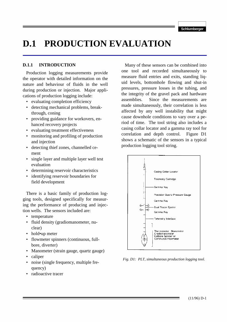
Many of these sensors can be combined intoone tool and recorded simultaneously tomeasure fluid entries and exits, standing liq-uid levels, bottomhole flowing and shut-inpressures, pressure losses in the tubing, andthe integrity of the gravel pack and hardwareassemblies. Since the measurements aremade simultaneously, their correlation is lessaffected by any well instability that mightcause downhole conditions to vary over a pe-riod of time. The tool string also includes acasing collar locator and a gamma ray tool forcorrelation and depth control. Figure D1shows a schematic of the sensors in a typicalproduction logging tool string.

Fig. D1: PLT, simultaneous production logging tool.

Introduction to Cased Hole Logging

(11/96) D-2

Production Logging ApplicationsA great value of production logs lies in their

ability to provide determinations of the dy-namic flow patterns of well fluids under sta-ble producing or injecting conditions. For anumber of reasons production data from othersources may be misleading. Some of thesereasons are:

• Surface measurements of pressures,temperatures, and flow rates are notnecessarily diagnostic of what is hap-pening in the well.

• Fluid flow outside the presumed paths,such as through cement channels in theannulus, can only be detected by pro-duction logs.

• Zone-by-zone measurements of perfo-rating efficiency, impractical except byproduction logs, are often necessary toidentify the actual producing or re-ceiving intervals.

• Zone-by-zone measurements of pres-sure and flow rate can be used to de-termine the average pressure and theproductivity index of each producing orinjected interval.

Production logs therefore have useful appli-cation in two broad areas: evaluation of wellperformance with respect to the reservoir andanalysis of mechanical problems.

Well PerformanceIn a producing well, production logs can

determine which perforated zones are givingup fluids, ascertain the types and proportionsof the fluids, and measure the downhole con-ditions of temperature and pressure, and therates at which the fluids are flowing. If thiefzones or other unwanted downhole fluid cir-culations exist, they can be pinpointed.

Injection wells are especially well adaptedto production log analysis because the fluid ismonophasic and of a known and controlledtype. The objective of logging is to locate thezones taking fluid and to detect lost injectionthrough the casing annulus.

Job PlanningPlanning is the most important facet of a

successful production logging job. Close co-ordination between Schlumberger engineersand well operators is essential.

Planning should start with defining andanalyzing the expected downhole injection orproduction rates, pressures, temperatures, andfluid types. This analysis will determine thetool types and resolutions needed to solve theproblem. The presence of H2S and CO2

should also be considered. The following in-formation is required to plan the operation:

• a detailed well sketch• Christmas tree specifications for rigup• sand or formation fines production• presence of paraffin or scale deposits• knowledge of whether the well was hy-

draulically fractured and/or acidized• frac balls usage• reservoir data, reservoir and fluid

properties• production history.

Before the production logging operation isattempted, the operator should verify that thewell conditions are acceptable by running adummy tool to the bottom to determine ifthere are any obstacles. Any problems shouldbe remedied before the logging operation isstarted.

Schlumberger

(11/96) D-3

Time allocation is an important considera-tion for production logging operations - par-ticularly in high pressure operations. Surveyscan frequently be run more safely in daylight.If not this may dictate the use of speciallighting equipment for lengthy operations.

Well ProblemsIn the absence of knowledge to the contrary,

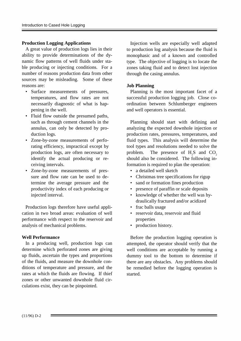
it is assumed that the well has hydraulic integ-rity, and that the fluids are going where theybelong; often, this assumption is wrong. Ex-amples include: casing leaks, tubing leaks,packer leaks, communication through the an-nulus due to poor cement, and thief zones.Figure D2 shows how these conditions canlead to misleading conclusions when well per-formance data come from surface measure-ments alone. Solutions to these and otherwell problems can be found by the integrationand interpretation of production log data.

We will cover the various production log-ging tools and how each is interpreted indi-vidually. Once the measurement made byeach PL sensor is understood we are thenbetter able to combine them for a better inter-pretation. In the interpretation section we willcover the various flow regimes occurring inthe wellbore during production.

Fig. D2: Mechanical well problems.

Introduction to Cased Hole Logging

(11/96) D-4

Schlumberger

(11/96) D-5

D.2 FLOWMETER TOOLS

Flow VelocityFlowmeter spinner tools and radioactive

tracer tools are usually used to measure flowvelocity. Under certain conditions, the fluiddensity and temperature tools can be used toestimate flow rates but their use for this pur-pose is much less common.

Spinner Flowmeter ToolsSpinner flowmeters all incorporate some

type of impeller that is rotated by fluid mov-ing relative to the impeller. The impellercommonly turns on a shaft with magnets thatrotate inside a coil. The induced current inthe coil is monitored and converted to a spin-ner speed in revolutions per second. Thisspinner speed is then converted to fluid ve-locity (flow rate).

D.2.1 CONTINUOUS FLOWMETERTOOL

The continuous flowmeter tool has an im-peller mounted inside the tool, or in some ver-sions, at the end of it (Figure D3). The mostcommon tool diameter is 42.9 mm (1 11/16 in)with the spinner being smaller. The continu-ous flowmeter is most often run in tubingwhere the fluid velocities are high and thefluids tend to be a homogeneous mixture.The spinner covers a much larger percentageof the cross-sectional flowing area than incasing and tends to average the fluid velocityprofile.

Fig.D3: Continuous Flowmeter.

Introduction to Cased Hole Logging

(11/96) D-6

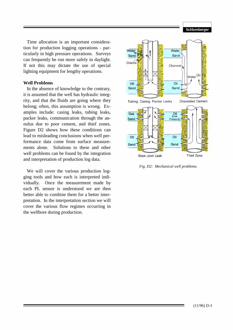
Fig.D4: Fullbore spinner flowmeter tool.

D.2.2 FULLBORE SPINNER TOOL(FBS)

The FBS tool is probably the most com-monly run spinner tool. The tool collapses totraverse the tubing and opens inside casing forlogging purposes. The large cross-sectionalarea of the spinner tends to correct for fluidvelocity profiles and multiphase flow effects.A schematic of the FBS tool, in both the col-lapsed, through-tubing and opened, below-tubing, configuration is shown in Figure D4.

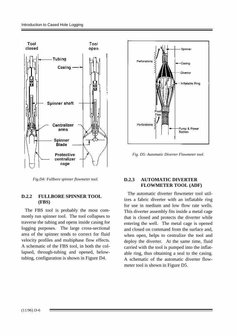
Fig. D5: Automatic Diverter Flowmeter tool.

D.2.3 AUTOMATIC DIVERTERFLOWMETER TOOL (ADF)

The automatic diverter flowmeter tool util-izes a fabric diverter with an inflatable ringfor use in medium and low flow rate wells.This diverter assembly fits inside a metal cagethat is closed and protects the diverter whileentering the well. The metal cage is openedand closed on command from the surface and,when open, helps to centralize the tool anddeploy the diverter. At the same time, fluidcarried with the tool is pumped into the inflat-able ring, thus obtaining a seal to the casing.A schematic of the automatic diverter flow-meter tool is shown in Figure D5.

Schlumberger

(11/96) D-7

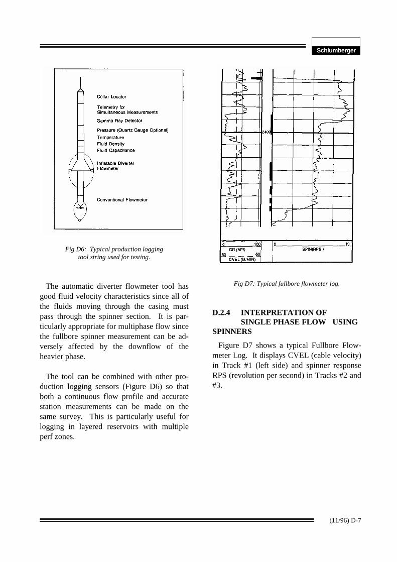
Fig D6: Typical production loggingtool string used for testing.

The automatic diverter flowmeter tool hasgood fluid velocity characteristics since all ofthe fluids moving through the casing mustpass through the spinner section. It is par-ticularly appropriate for multiphase flow sincethe fullbore spinner measurement can be ad-versely affected by the downflow of theheavier phase.

The tool can be combined with other pro-duction logging sensors (Figure D6) so thatboth a continuous flow profile and accuratestation measurements can be made on thesame survey. This is particularly useful forlogging in layered reservoirs with multipleperf zones.

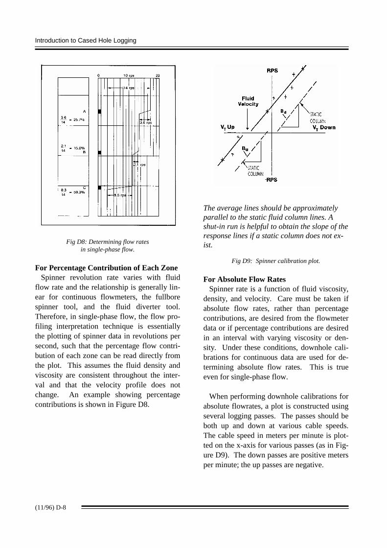
Fig D7: Typical fullbore flowmeter log.

D.2.4 INTERPRETATION OFSINGLE PHASE FLOW USING

SPINNERS

Figure D7 shows a typical Fullbore Flow-meter Log. It displays CVEL (cable velocity)in Track #1 (left side) and spinner responseRPS (revolution per second) in Tracks #2 and#3.

Introduction to Cased Hole Logging

(11/96) D-8

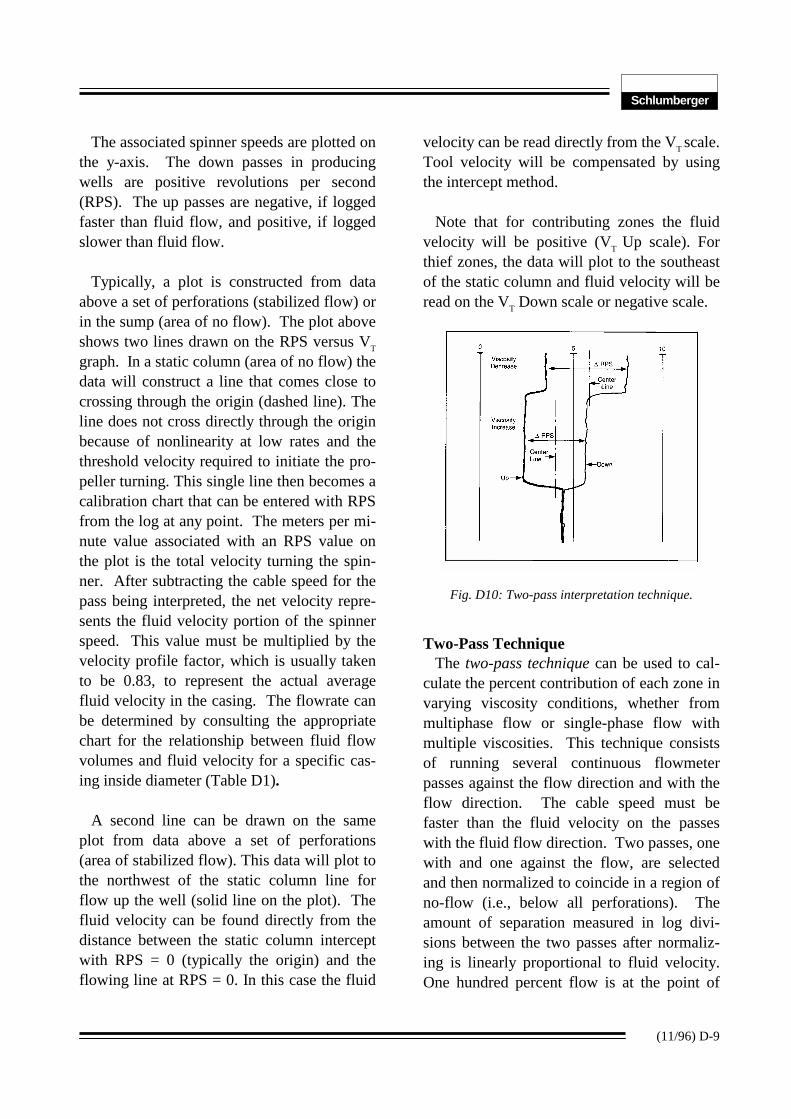
Fig D8: Determining flow ratesin single-phase flow.

For Percentage Contribution of Each ZoneSpinner revolution rate varies with fluid

flow rate and the relationship is generally lin-ear for continuous flowmeters, the fullborespinner tool, and the fluid diverter tool.Therefore, in single-phase flow, the flow pro-filing interpretation technique is essentiallythe plotting of spinner data in revolutions persecond, such that the percentage flow contri-bution of each zone can be read directly fromthe plot. This assumes the fluid density andviscosity are consistent throughout the inter-val and that the velocity profile does notchange. An example showing percentagecontributions is shown in Figure D8.

The average lines should be approximatelyparallel to the static fluid column lines. Ashut-in run is helpful to obtain the slope of theresponse lines if a static column does not ex-ist.

Fig D9: Spinner calibration plot.

For Absolute Flow RatesSpinner rate is a function of fluid viscosity,

density, and velocity. Care must be taken ifabsolute flow rates, rather than percentagecontributions, are desired from the flowmeterdata or if percentage contributions are desiredin an interval with varying viscosity or den-sity. Under these conditions, downhole cali-brations for continuous data are used for de-termining absolute flow rates. This is trueeven for single-phase flow.

When performing downhole calibrations forabsolute flowrates, a plot is constructed usingseveral logging passes. The passes should beboth up and down at various cable speeds.The cable speed in meters per minute is plot-ted on the x-axis for various passes (as in Fig-ure D9). The down passes are positive metersper minute; the up passes are negative.

Schlumberger

(11/96) D-9

The associated spinner speeds are plotted onthe y-axis. The down passes in producingwells are positive revolutions per second(RPS). The up passes are negative, if loggedfaster than fluid flow, and positive, if loggedslower than fluid flow.

Typically, a plot is constructed from dataabove a set of perforations (stabilized flow) orin the sump (area of no flow). The plot aboveshows two lines drawn on the RPS versus VT

graph. In a static column (area of no flow) thedata will construct a line that comes close tocrossing through the origin (dashed line). Theline does not cross directly through the originbecause of nonlinearity at low rates and thethreshold velocity required to initiate the pro-peller turning. This single line then becomes acalibration chart that can be entered with RPSfrom the log at any point. The meters per mi-nute value associated with an RPS value onthe plot is the total velocity turning the spin-ner. After subtracting the cable speed for thepass being interpreted, the net velocity repre-sents the fluid velocity portion of the spinnerspeed. This value must be multiplied by thevelocity profile factor, which is usually takento be 0.83, to represent the actual averagefluid velocity in the casing. The flowrate canbe determined by consulting the appropriatechart for the relationship between fluid flowvolumes and fluid velocity for a specific cas-ing inside diameter (Table D1).

A second line can be drawn on the sameplot from data above a set of perforations(area of stabilized flow). This data will plot tothe northwest of the static column line forflow up the well (solid line on the plot). Thefluid velocity can be found directly from thedistance between the static column interceptwith RPS = 0 (typically the origin) and theflowing line at RPS = 0. In this case the fluid

velocity can be read directly from the VT scale.Tool velocity will be compensated by usingthe intercept method.

Note that for contributing zones the fluidvelocity will be positive (VT Up scale). Forthief zones, the data will plot to the southeastof the static column and fluid velocity will beread on the VT Down scale or negative scale.

Fig. D10: Two-pass interpretation technique.

Two-Pass TechniqueThe two-pass technique can be used to cal-

culate the percent contribution of each zone invarying viscosity conditions, whether frommultiphase flow or single-phase flow withmultiple viscosities. This technique consistsof running several continuous flowmeterpasses against the flow direction and with theflow direction. The cable speed must befaster than the fluid velocity on the passeswith the fluid flow direction. Two passes, onewith and one against the flow, are selectedand then normalized to coincide in a region ofno-flow (i.e., below all perforations). Theamount of separation measured in log divi-sions between the two passes after normaliz-ing is linearly proportional to fluid velocity.One hundred percent flow is at the point of

Introduction to Cased Hole Logging

(11/96) D-10

maximum deflection, which is usually aboveall perforations. Thief zones complicate theinterpretation somewhat, but the principle re-mains the same.

A distinct advantage of this technique is thatit cancels the effect of viscosity changes.These changes are essentially shifts in RPSreadings in the same amount and direction onboth passes. Thus, the separation remains in-dependent of viscosity effects. If the center-line is defined as a line halfway between thetwo curves, a centerline shift to the right is aviscosity decrease; a centerline shift to the leftis a viscosity increase (Figure D10). If abso-lute fluid velocity is desired from the two-passtechnique, and if multiple calibration passeshave been run, it can be computed from thefollowing equation:

vf = 0.83 [(∆RPS) / (Bu + Bd)],

where:

Bu is the up calibration line slope inrps per meter per minute.Bd is the down calibration line slopein rps per meter per minute.Bu and Bd can, and often will, beslightly different numerically.∆RPS is the amount of separationbetween up and down passes in RPS.

Although the foregoing comments focus onfluid viscosity changes, the ef-fects/assumptions regarding fluid densitychanges are similar but opposite in effect.Fluid velocity can be converted to flow ratesin barrels per day with production log chart 6-10 (see Table D1).

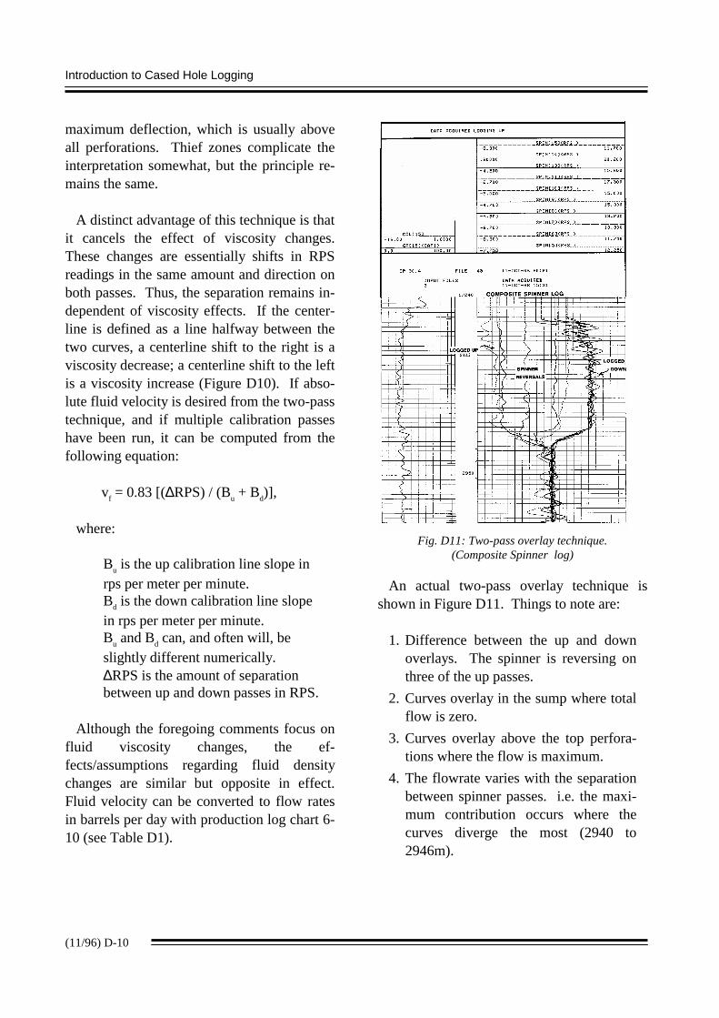
Fig. D11: Two-pass overlay technique.(Composite Spinner log)

An actual two-pass overlay technique isshown in Figure D11. Things to note are:

1. Difference between the up and downoverlays. The spinner is reversing onthree of the up passes.

2. Curves overlay in the sump where totalflow is zero.

3. Curves overlay above the top perfora-tions where the flow is maximum.

4. The flowrate varies with the separationbetween spinner passes. i.e. the maxi-mum contribution occurs where thecurves diverge the most (2940 to2946m).

Schlumberger

(11/96) D-11

D.3 TRACER TOOLS

Tracer tools can be placed into two basiccategories. These are:

1. Gamma ray tools that do not have down-hole ejectors for releasing radioactive ma-terial, and

2. Gamma ray tools that have downholeejectors in combination with multiplegamma ray detectors.

The first category is comprised of tools thatare essentially the same as those used foropenhole logging. These are usually smallerdiameter tools for through-tubing application.The more common sizes are 35mm and43mm. In addition to flow profiling with thecontrolled time technique and traditionalopenhole logging, these tools are often usedfor channel detection by comparing loggingruns made before and after injecting fluidscontaining radioactive material into the well.The difference in the two runs will identifywhere radioactive materials are present. Ifradioactive material is present at any pointother than the perforated intervals, channelingor vertical fracturing is likely.

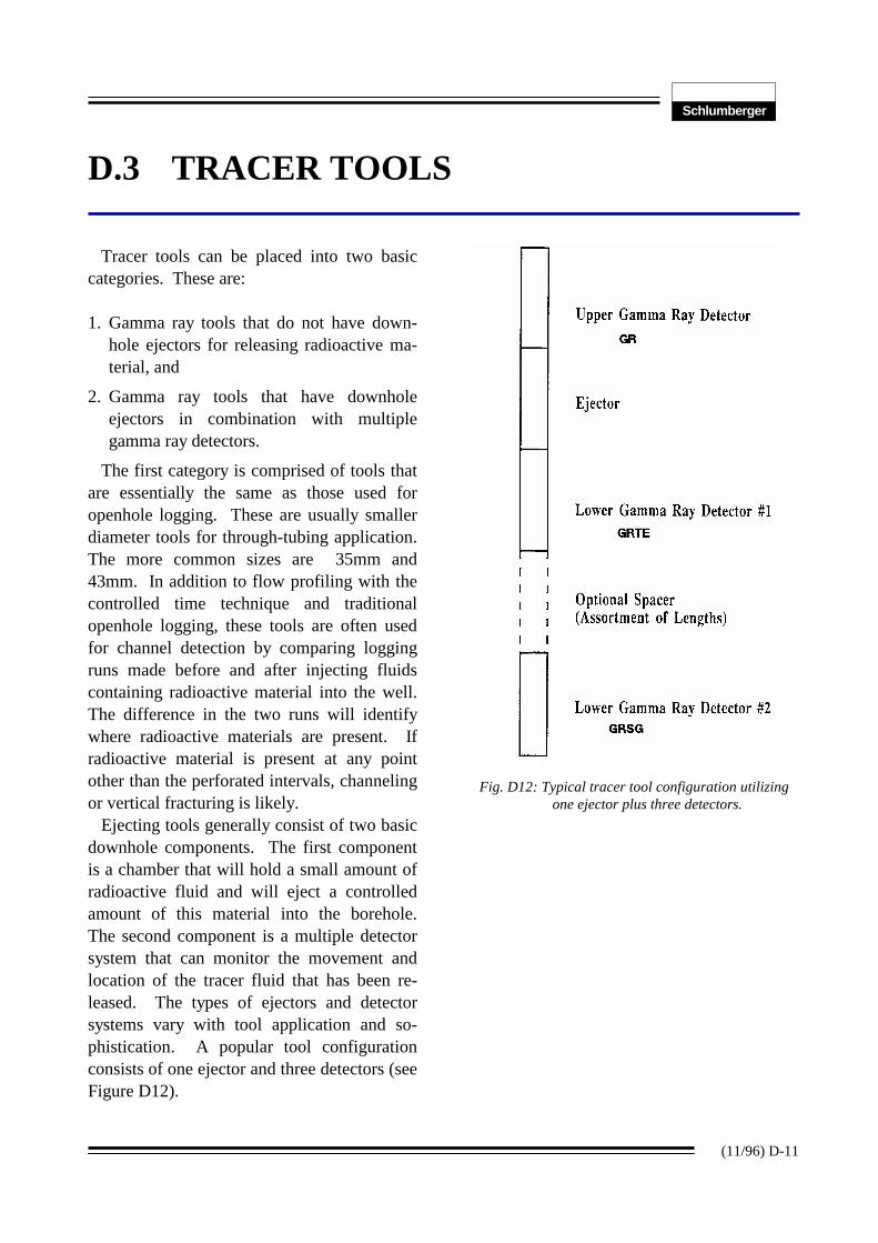
Ejecting tools generally consist of two basicdownhole components. The first componentis a chamber that will hold a small amount ofradioactive fluid and will eject a controlledamount of this material into the borehole.The second component is a multiple detectorsystem that can monitor the movement andlocation of the tracer fluid that has been re-leased. The types of ejectors and detectorsystems vary with tool application and so-phistication. A popular tool configurationconsists of one ejector and three detectors (seeFigure D12).

Fig. D12: Typical tracer tool configuration utilizingone ejector plus three detectors.

Introduction to Cased Hole Logging

(11/96) D-12

The tool configuration depends on the fluidflow direction. If logging an injection well,the configuration will normally be one detec-tor above the ejector and two spaced detectorsbelow. In a producing situation, two detectorsare placed above the ejector and one detectoris placed below. The purpose of the singledetector on the opposite side of the ejectorfrom the flow direction is for detecting unex-pected flow reversals produced by thief zonesand for identifying channels behind casing,where fluid is flowing opposite the directionof the wellbore fluids. The purpose of the twoadjacent detectors is for flow profiling as afunction of flow time between the two detec-tors.

The principle of ejector tracer logging is thereleasing of a radioactive isotope that dis-solves in the wellbore and becomes part of thewellbore fluid. The tracer material moves atthe same velocity as the wellbore fluid. Ameasurement of the elapsed detection timebetween the two detectors, along with knowl-edge of the tool configuration, is enough in-formation for computing fluid flowrate. Thisassumes, of course, that the tool is not mov-ing. Unlike the controlled time survey, thetool diameter must be considered in theflowrate computation because it subtractsfrom the casing internal cross-sectional area.

Tracer Flow Rate Formula:

spacing x (π/4)(dh2-dtool

2) x 1440 q = time x (1/60)Where:

q is the flowrate in m3/day.spacing is the distance betweenthe two detectors in meters.dh is the casing inside diameterin meters.dtool is the tool diameter in meters.time is the elapsed time betweendetections in seconds.

For example:

Casing ID = 161.700mm = 0.161700m.Tool OD = 34.925mm = 0.034925m.

For near detector to far detector, with spac-ing 1.4986m, and elapsed detection time of 15seconds:

q = 169 m3/day

The sensitivity of the detectors to gammarays allows the system to monitor radiationchanges inside the casing wall and outside thecasing near the casing wall. The actual depthof investigation of the gamma ray detectordepends on the type of detector, and the mag-nitude of the radiation. In most cases, it canbe estimated at 0.3 meters.

Schlumberger

(11/96) D-13

Water, oil, or gas soluble tracer materialscan be used. Water soluble material is themost common.

Some fluid flow applications of radioactivetracer logging are:

- To check for packer, casing, or tubingleaks;

- To identify channeling;

- To establish injection profiles on injec-tor wells;

- To imply production profiles from injec-tion profiles on production wells duringinjection testing; and

- To establish flow profiles in low flow areasof producing wells. (Tracer logging inproducing wells requires special consid-erations.)

Most of these applications require loggingtechniques and interpretation methods uniqueto the problem.

Radioactive tracer surveys are not routinelyrun in producing wells because of the compli-cations of produced radioactive fluid andmultiphase flow effects. Therefore, the mainapplication of this technique is in injectionwells.

As a general rule, the flowmeter gives moreaccurate results in high flow rates and the ra-dioactive tracer technique provides better re-sults in flow rates less than about 100 B/D.

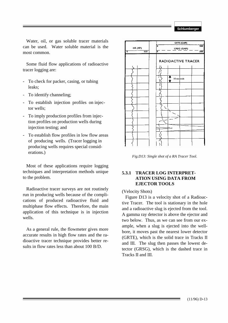
Fig.D13: Single shot of a RA Tracer Tool.

5.3.1 TRACER LOG INTERPRET-ATION USING DATA FROM EJECTOR TOOLS

(Velocity Shots)Figure D13 is a velocity shot of a Radioac-

tive Tracer. The tool is stationary in the holeand a radioactive slug is ejected from the tool.A gamma ray detector is above the ejector andtwo below. Thus, as we can see from our ex-ample, when a slug is ejected into the well-bore, it moves past the nearest lower detector(GRTE), which is the solid trace in Tracks IIand III. The slug then passes the lowest de-tector (GRSG), which is the dashed trace inTracks II and III.

Introduction to Cased Hole Logging

(11/96) D-14

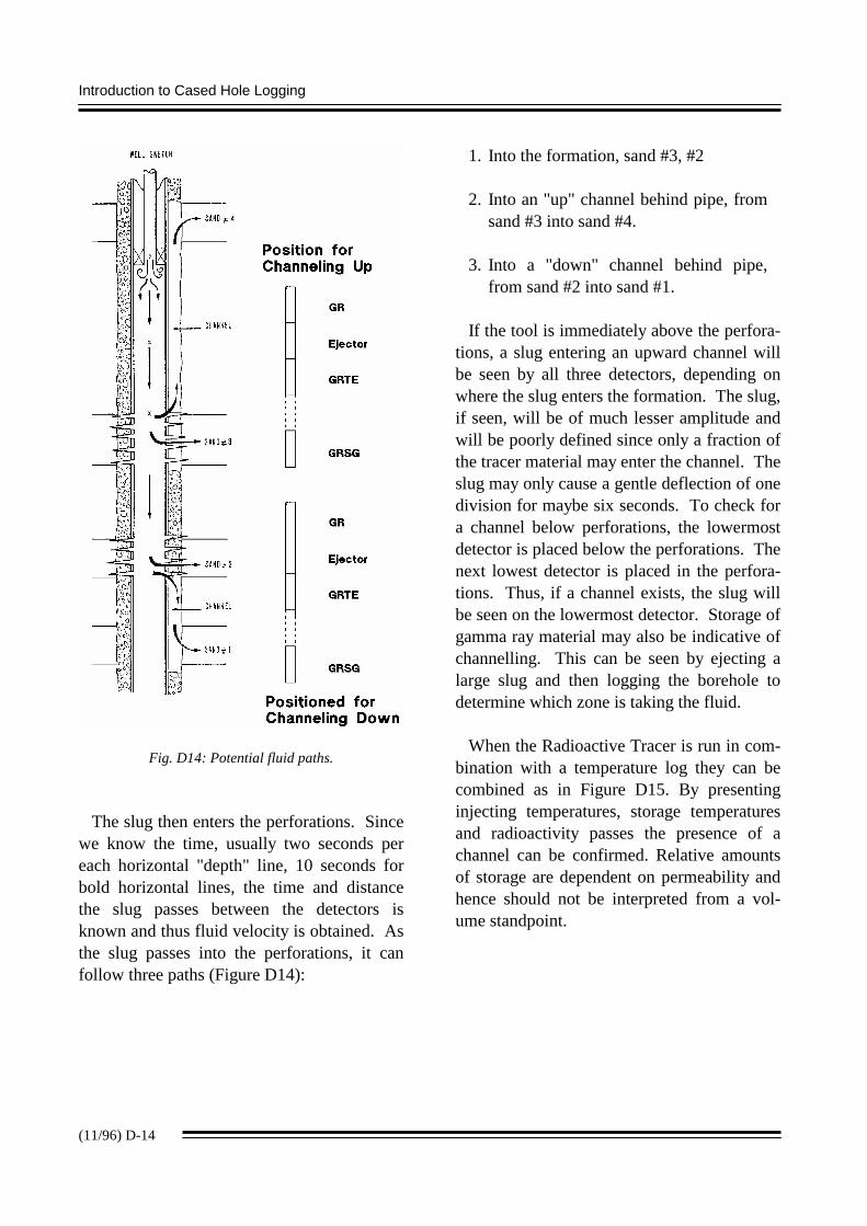
Fig. D14: Potential fluid paths.

The slug then enters the perforations. Sincewe know the time, usually two seconds pereach horizontal "depth" line, 10 seconds forbold horizontal lines, the time and distancethe slug passes between the detectors isknown and thus fluid velocity is obtained. Asthe slug passes into the perforations, it canfollow three paths (Figure D14):

1. Into the formation, sand #3, #2

2. Into an "up" channel behind pipe, fromsand #3 into sand #4.

3. Into a "down" channel behind pipe,from sand #2 into sand #1.

If the tool is immediately above the perfora-tions, a slug entering an upward channel willbe seen by all three detectors, depending onwhere the slug enters the formation. The slug,if seen, will be of much lesser amplitude andwill be poorly defined since only a fraction ofthe tracer material may enter the channel. Theslug may only cause a gentle deflection of onedivision for maybe six seconds. To check fora channel below perforations, the lowermostdetector is placed below the perforations. Thenext lowest detector is placed in the perfora-tions. Thus, if a channel exists, the slug willbe seen on the lowermost detector. Storage ofgamma ray material may also be indicative ofchannelling. This can be seen by ejecting alarge slug and then logging the borehole todetermine which zone is taking the fluid.

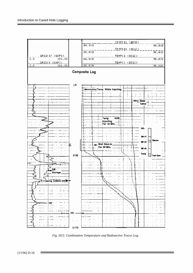
When the Radioactive Tracer is run in com-bination with a temperature log they can becombined as in Figure D15. By presentinginjecting temperatures, storage temperaturesand radioactivity passes the presence of achannel can be confirmed. Relative amountsof storage are dependent on permeability andhence should not be interpreted from a vol-ume standpoint.

Schlumberger

(11/96) D-15

Controlled Time SurveyThe controlled time method qualitatively

detects the flow of fluids up or down the hole,either in the casing or in the annulus. Figure 5shows an example of the controlled-time Ra-dioactive Tracer Survey. In this case radioac-tive material was ejected at the bottom of thetubing and successive runs were made withthe gamma ray tool. The times of the injec-tion and of each log run were carefully noted.

The radioactive slug (points a, c, e, and h)may be seen to move down the casing. Afterentering the perforations opposite sand 3, apart of the radioactive slug (points f, j, h, andv) channels up the casing annulus to sand 4.After entering at sand 2, part of the radioac-tive slug (points l and p) channels down thecasing annulus to sand 1. Fluid appears to beentering sand 3 because of the stationaryreadings at points i, m, and q. And finally,some radioactive material is trapped in a tur-bulence pattern just below the tubing asshown by points b, d, g, and k.

Introduction to Cased Hole Logging

(11/96) D-16

Fig. D15: Combination Temperature and Radioactive Tracer Log.

Schlumberger

(11/96) D-17

Fig. D16: Radioactive tracer survey: timed runs analysis.

Introduction to Cased Hole Logging

(11/96) D-18

Schlumberger

(11/96) D-19

D.4 FLUID DENSITY TOOLS

There are two major types of fluid densitytools:

1. Gradiomanometer fluid density tool

2. Nuclear fluid density tool (gamma ray ab-sorption)

A third tool type works on a principle otherthan fluid density, it is the capacitance or wa-tercut tool.

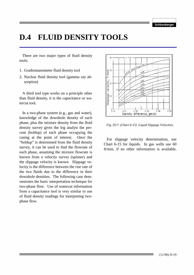
In a two-phase system (e.g., gas and water),knowledge of the downhole density of eachphase, plus the mixture density from the fluiddensity survey gives the log analyst the per-cent (holdup) of each phase occupying thecasing at the point of interest. Once the“holdup” is determined from the fluid densitysurvey, it can be used to find the flowrate ofeach phase, assuming the mixture flowrate isknown from a velocity survey (spinner) andthe slippage velocity is known. Slippage ve-locity is the difference between the rise rate ofthe two fluids due to the difference in theirdownhole densities. The following case dem-onstrates the basic interpretation technique fortwo-phase flow. Use of watercut informationfrom a capacitance tool is very similar to useof fluid density readings for interpreting two-phase flow.

Fig. D17: (Chart 6-15) Liquid Slippage Velocities.

For slippage velocity determination, useChart 6-15 for liquids. In gas wells use 60ft/min, if no other information is available.

Introduction to Cased Hole Logging

(11/96) D-20

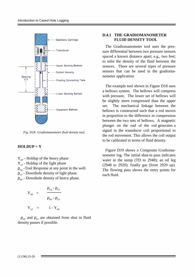
Fig. D18: Gradiomanometer fluid density tool.

HOLDUP = Y

YHP - Holdup of the heavy phaseYLP - Holdup of the light phaseρlog -Tool Response at any point in the well.ρLP - Downhole density of light phase.ρHP - Downhole density of heavy phase.

ρlog - ρLP

YHP =ρHP - ρLP

YLP = 1 - YHP

ρHP and ρLP are obtained from shut in fluiddensity passes if possible.

D.4.1 THE GRADIOMANOMETERFLUID DENSITY TOOL

The Gradiomanometer tool uses the pres-sure differential between two pressure sensorsspaced a known distance apart; e.g., two feet;to infer the density of the fluid between thesensors. There are several types of pressuresensors that can be used in the gradioma-nometer application.

The example tool shown in Figure D18 usesa bellows system. The bellows will compresswith pressure. The lower set of bellows willbe slightly more compressed than the upperset. The mechanical linkage between thebellows is constructed such that a rod movesin proportion to the difference in compressionbetween the two sets of bellows. A magneticplunger on the end of the rod generates asignal in the transducer coil proportional tothe rod movement. This allows the coil outputto be calibrated in terms of fluid density.

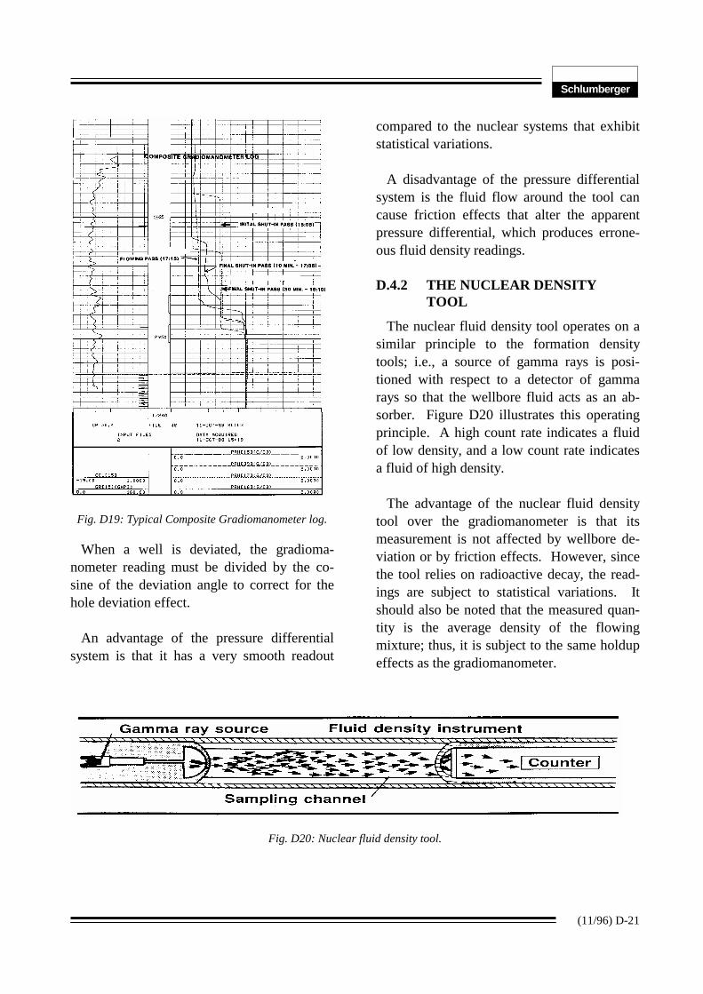
Figure D19 shows a Composite Gradioma-nometer log. The initial shut-in pass indicateswater in the sump (TD to 2948); an oil leg(2948 to 2920); finally gas (from 2920 up).The flowing pass shows the entry points foreach fluid.

Schlumberger

(11/96) D-21

Fig. D19: Typical Composite Gradiomanometer log.

When a well is deviated, the gradioma-nometer reading must be divided by the co-sine of the deviation angle to correct for thehole deviation effect.

An advantage of the pressure differentialsystem is that it has a very smooth readout

compared to the nuclear systems that exhibitstatistical variations.

A disadvantage of the pressure differentialsystem is the fluid flow around the tool cancause friction effects that alter the apparentpressure differential, which produces errone-ous fluid density readings.

D.4.2 THE NUCLEAR DENSITYTOOL

The nuclear fluid density tool operates on asimilar principle to the formation densitytools; i.e., a source of gamma rays is posi-tioned with respect to a detector of gammarays so that the wellbore fluid acts as an ab-sorber. Figure D20 illustrates this operatingprinciple. A high count rate indicates a fluidof low density, and a low count rate indicatesa fluid of high density.

The advantage of the nuclear fluid densitytool over the gradiomanometer is that itsmeasurement is not affected by wellbore de-viation or by friction effects. However, sincethe tool relies on radioactive decay, the read-ings are subject to statistical variations. Itshould also be noted that the measured quan-tity is the average density of the flowingmixture; thus, it is subject to the same holdupeffects as the gradiomanometer.

Fig. D20: Nuclear fluid density tool.

Introduction to Cased Hole Logging

(11/96) D-22

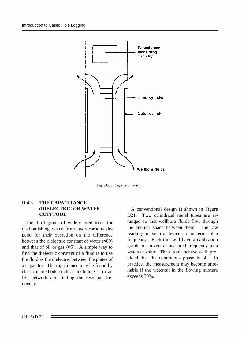
Fig. D21: Capacitance tool.

D.4.3 THE CAPACITANCE(DIELECTRIC OR WATER-CUT) TOOL

The third group of widely used tools fordistinguishing water from hydrocarbons de-pend for their operation on the differencebetween the dielectric constant of water (≈80)and that of oil or gas (≈6). A simple way tofind the dielectric constant of a fluid is to usethe fluid as the dielectric between the plates ofa capacitor. The capacitance may be found byclassical methods such as including it in anRC network and finding the resonant fre-quency.

A conventional design is shown in FigureD21. Two cylindrical metal tubes are ar-ranged so that wellbore fluids flow throughthe annular space between them. The rawreadings of such a device are in terms of afrequency. Each tool will have a calibrationgraph to convert a measured frequency to awatercut value. These tools behave well, pro-vided that the continuous phase is oil. Inpractice, the measurement may become unre-liable if the watercut in the flowing mixtureexceeds 30%.