optimal herbicide use in conservation tillage systems
TRANSCRIPT

OPTIMAL HERBICIDE USE IN CONSERVATION TILLAGESYSTEMS
A Research Report
Presented to
The Technology and Development Sub Program
of
The Soil and Water Environment Enhancement Program
by
JAMES E. SHAW,
CLARENCE J. SWANTON
and
VIKRAM S. MALIK
In fulfilment of requirements
for ted contract 01686-7-0286
March, 1991
ATTENTION
THE HERBICIDE RECOMMENDATIONS MADE IN
THIS REPORT DO NOT NECESSARILY REPRESENT
REGISTERED TREATMENTS FOR USE IN ONTARIO.
THESE RECOMMENDATIONS ARE ONLY FOR
RESEARCH PURPOSES AT THIS TIME.

i
PROJECT PERSONNEL
RESEARCHERS
JAMES E. SHAW CLARENCE J. SWANTON
Weed Scientist, Associate Professor,
Ridgetown College of Crop Science,
Agricultural Technology, University of Guelph,
Ridgetown, Ontario, Canada. Guelph, Ontario, Canada.
FINANCIAL OFFICER PROJECT LEADER
DON W. TAYLOR, RUDOLF H. BROWN,
RCAT, Ridgetown, Ontario. RCAT, Ridgetown, Ontario.
REPORT WRITER & COMPILER
VIKRAM S. MALIK
University of Guelph

ii
ACKNOWLEDGEMENTS
The authors express their gratitude to the Technology Evaluation and Development (TED)
sub-program of the Soil and Water Environmental Enhancement Programme (SWEEP) for their
financial support. The financial management of Mr. D.W. Taylor, Director, Ridgetown College of
Agricultural Technology is also gratefully acknowledged.
The authors express their appreciation to Mr. R.H. Brown for his numerous contributions
to this project.
The Authors also wishes to thank Mr. Dave Bilyae, Kevin Chandler, Bob Stone and all
summer students who helped in conducting field experiments. The valuable research by graduate
students Mr. Godwin Aflakpui, Allen Eadie and Mike Walker towards various objectives in this
project is also highly appreciated. The authors also thank Mr. Don Lobb, Art Wardle, Jack Rigby,
Al and Paul Jones who provided land and helpful comments in order to ensure the applicability of
the experiments to the on-farm situations.
The authors also sincerely acknowledge Dr. A. Weersink for his supervision of Mr. Mike
Walker's research and thesis writing.

iii
TABLE OF CONTENTS
Page
Research Personnel ...................................... i
Acknowledgements ......................................... ii
Table of Contents ........................................ iii
Executive Summary ........................................ v
1.0 INTRODUCTION ................................... 1
2.0 WEATHER DATA ................................... 5
3.0 BURNDOWN AND RESIDUAL HERBICIDES FOR LEGUME AND CEREAL COVER CROP PLANTEDIN CORN AND SOYBEANS ........................... 7
3.1 Methods and Materials .......................... 93.2 Alfalfa burndown in soybeans ................... 123.3 Winter wheat burndown in soybeans .............. 163.4 Winter wheat burndown .......................... 193.5 Red clover burndown in corn .................... 213.6 Alfalfa burndown in corn ....................... 243.7 Recommendations ................................ 38
4.0 ANTAGONISM OF BURNDOWN HERBICIDES WITH RESIDUAL HERBICIDES IN CONSERVATION TILLAGE SYSTEMS ............. 41
4.1 Methods and Materials .......................... 424.2 Paraquat and glufosinate antagonism with residual herbicides in corn ..... 464.3 Glyphosate antagonism with residual herbicides in corn ............................. 514.4 Paraquat and glufosinate antagonism with residual herbicides in soybeans . 564.5 Glyphosate antagonism with residual herbicides in soybeans ...................... 614.6 Compatibility of burndown and residual herbicides for quackgrass control 664.7 Recommendations ................................ 69
iv
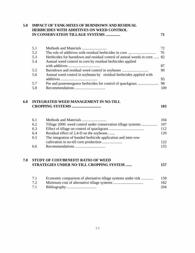
5.0 IMPACT OF TANK-MIXES OF BURNDOWN AND RESIDUAL HERBICIDES WITH ADDITIVES ON WEED CONTROL
IN CONSERVATION TILLAGE SYSTEMS ................ 71
5.1 Methods and Materials .......................... 725.2 The role of additives with residual herbicides in corn ............................. 765.3 Herbicides for burndown and residual control of annual weeds in corn ...... 825.4 Annual weed control in corn by residual herbicides applied
with additives ................................. 875.5 Burndown and residual weed control in soybeans ............................ 905.6 Annual weed control in soybeans by residual herbicides applied with
additives ...................................... 955.7 Pre and postemergence herbicides for control of quackgrass ...................... 985.8 Recommendations ................................ 100
6.0 INTEGRATED WEED MANAGEMENT IN NO-TILLCROPPING SYSTEMS ............................... 103
6.1 Methods and Materials .......................... 1046.2 Tillage 2000: weed control under conservation tillage systems ................. 1076.3 Effect of tillage on control of quackgrass ..................................... 1126.4 Residual effect of 2,4-D on the soybeans ....... 1206.5 The integration of banded herbicide application and inter-row
cultivation in no-till corn production ..................... 1226.6 Recommendations ................................ 155
7.0 STUDY OF COST/BENEFIT RATIO OF WEEDSTRATEGIES UNDER NO-TILL CROPPING SYSTEM ....... 157
7.1 Economic comparison of alternative tillage systems under risk ............. 1587.2 Minimum cost of alternative tillage systems ................................ 1827.1 Bibliography ............................... 204

v
EXECUTIVE SUMMARY
The goal of this study was to develop weed control recommendations for farmers utilizing
conservation tillage systems. Efforts were directed towards optimizing herbicide selection, dosage
and timing of application in order to achieve effective weed control. Moreover, research was also
conducted to optimize herbicide inputs by developing an integrated weed management system for
no-till corn. An economic and risk management study of weed control measures was also
completed.
The results of this study will provide weed control and specific crop recommendations for
farmers using conservation tillage. This information will facilitate the acceptance of conservation
tillage practices within the Ontario farming community.
Field experiments were conducted from 1987 to 1990 to address the specific objective
outlined in this report. Our findings included:
1. Currently recommended herbicides and herbicide combinations provided excellent broad-
spectrum weed control in all tillage systems tested.
2. Control of weeds in conservation tillage systems did not require higher dosages of
herbicides despite the presence of crop residue on the soil surface.
3. Perennial weeds can be effectively controlled and should not pose a significant threat to
successful crop production in conservation tillage systems.
4. The integration of banded herbicide applications, inter-row cultivation and reduced
herbicide dosage can be integrated as a weed control alternative for no-till corn . Adoption

vi
of these practices can reduce the total amount of herbicide applied into the environment by
60%.
5. An economic comparison of alternative tillage systems and weed control practices among
various tillage systems was completed. Optimum preemergence herbicide applications were
identified for both corn and soybeans grown under four different tillage systems. The
reductions in labour associated with the reduced tillage systems indicated that labour cost
were reduced by up to 61% annually when compared with an conventional tillage systems.
This saving in labour was illustrated as an opportunity cost associated with reduced tillage
systems on sandy soils. A sensitivity analysis between moldboard plough and no-till
indicated that no-till will dominate in risk preferring intervals, and an increase in no-till net
farm returns of $ 40 ha-1 would change dominance in favour of no-till among risk averse
individuals. It is possible for conservation tillage systems to dominate conventional tillage
systems, if proper weed control and crop production techniques are undertaken.

1
1.0 INTRODUCTION
Tillage has been used for centuries to prepare fields for cropping. Perhaps the most important
reason for tillage is for the preparation of a vegetation-free seedbed at planting. However, this
seedbed preparation exposes the soil to wind and water erosion.
A recent study in the Thames River basin in Ontario, Canada, indicated that up to 95% of total
nitrogen and 74% of the phosphorus found in the Thames river came from various diffuse source
inputs, especially agricultural farmland (Anonymous 1975). Most of these nutrients are strongly
attached to the soil particles. Their movement beyond farm boundaries was mainly attributed to the
eroded soil particles. In Ontario, total annual losses due to soil erosion were estimated to be $74
million (Wall and Driver 1982). These costs do not include the off-site effects on society.
Measurement of off-site erosion effects is very difficult to accomplish because it involves a number
of commodities for which price is not available. However, Fox and Dickson (1990) attempted to
provide a dollar value to some of these off-site losses in southern Ontario. In their conservative
estimation, the cost for sediments removal from public water supplies alone was around $10.2
million. They also estimated that total benefits to sport fishing of $35 million if all of the excess
sedimentation of lakes and rivers in southern Ontario is removed. Such issues are of major concern
to the agriculturalists, to the government and public in Canada. These issues have led research
workers to try alternative crop production systems.
It is now well established that extensive tillage practices are not a pre-requisite for crop
establishment. Recent advances in crop seeding with minimum soil disturbances and maintaining a
vegetation-free seedbed using herbicides opened a new avenue for successful crop production with
reduced erosions from farmers' fields. In this ongoing review, an attempt has been made to define

2
various conservation tillage systems employed in Ontario and their respective weed management
strategies.
Conservation tillage in Ontario has taken three main directions, minimum-till, ridge-till and no-
till. Minimum-tillage systems encompass several variations in tillage practices. Tillage, prior to
planting occurs even though the seedbed is left rough and covered to some degree by previous crop
residue. In this system weed control methods are very similar to those of conventional tillage. Early
weed suppression and crop establishment is enhanced by tillage prior to planting. Since tillage is still
an important component of the weed control system, the weed spectrum is usually not changed
drastically from what exists in the conventional system. The major difference between minimum-till
and conventional-till is the presence of previous crop residue. In minimum-tillage systems large
amounts of crop residue may interfere with good incorporation of herbicides. Soil type, amount and
type of crop residue, and incorporation equipment available determines the feasibility of the preplant
incorporation method of chemical weed control. If good herbicide incorporation cannot be achieved,
the grower is limited to preemergence and postemergence herbicide treatments. Crop residue, if
plentiful may also intercept large percentages of soil surface applied herbicides and prevent them from
being activated in the soil where they perform the function of destroying weed seedlings. Research
in this area indicates that normal rainfall washed herbicides off crop residues and into the soil where
they work. There is evidence in the literature that allelopathic chemicals produced in decaying crop
residue interfere with seedling growth and may contribute significantly to weed control. Our research
does not address these concepts. Basically, weed control in minimum-tillage is very similar to that
of conventional-tillage.
In ridge-till systems, when the basic ridge-till concepts are adhered to, early weed suppression
and crop establishment is enhanced by tillage during planting. The aggressive cultivation and ridging

3
procedure that follow provide a great deal of mechanical weed control. This system is well suited to
broadcast or band applications of preemergent or postemergent herbicides. Weed control in this
system requires the least amount of herbicide of any system provided seeding, cultivation and re-
ridging are timely and equipment is properly adjusted. If weed problems develop, they usually begin
in the side of the ridges where perennial weeds like dandelion gain a foothold. Moreover, if seeding
is delayed in the spring, winter annual and perennial weeds that grow rapidly early in the spring, may
be a problem. Fall application of herbicides, while these weeds are still actively growing, may be a
practical approach to their control.
If a grower chooses to go the no-till route, he faces the toughest challenge in weed control. In
this system, the farmer is depending entirely on herbicides to provide early weed control as well as
control of those weeds that emerge later after initial burndown. Because there is very little soil
disturbance, weeds that are characteristic to conventional tillage do not thrive and other weeds,
particularly perennials, may become the problem weeds. Weed emergence patterns are also very
different under no-till conditions. The herbicides available are fairly well understood in conventional
conditions, but they may perform quite differently when imposed into a no-till condition with large
amounts of crop residue and a very different and diverse weed spectrum.
Much of what is learned about individual herbicide performance, tank mixes, and sequential
herbicide applications in no-till, will also apply to the other forms of conservation tillage. Thus, our
approach to weed control in conservation tillage has been to work primarily with no-till hoping that
knowledge gained can have direct application to ridge-till and minimum-till systems.
Our main efforts have been directed at evaluating herbicides, herbicide tank-mixtures and
sequential treatments, currently being used in conventional-till systems for their suitability in no-till
system. Many of the herbicides being evaluated are currently registered for use in conventional

4
production systems and may require slight label modifications for use in conservation-tillage systems.
Growers prefer to make as few trips across their fields as possible and are anxious to combine
burndown and residual herbicide treatments into one applications. Our aim has been to evaluate this
concept from the point-of-view of cost, efficacy, and crop safety. Therefore, the objectives of this
study were to determine:
1. the effectiveness of various herbicides for burndown of cover crops tank-mixed with residual
preemergence herbicides for annual weed control in corn and soybeans.
2. the interaction (antagonism) of various burndown herbicides tank-mixed with residual
preemergence herbicides for annual weed control in corn and soybeans grown in various
conservation tillage systems.
3. the effect of various additives on the burndown effects of tank-mixes of herbicides in
conservation tillage in a corn and soybeans crop.
4. the benefits of fall application of herbicides for control of weeds in a corn and soybeans crop
grown in a minimum tillage system†.
5. the various aspects of an integrated weed management in no-till cropping system.
6. the cost/benefit ratio and associated risk of weed control strategies under various tillage
systems.
†
Two experiments were conducted under objective 4 and are being summarized as experiment 3.6 on
page 24 and experiment 5.7 on page 98.
2.0 WEATHER DATA

5
Table 1. Average monthly rainfall accumulation in 1987, 1988, 1989 and 1990 at DealtownResearch Station.
______________________________________________________________________________ Precipitation
1987 1988 1989 1990 10 year average
______________________________________________________________________________ ________________________ mm ____________________________
April 59.0 45.5 45.6 44.1 81.2May 4.8 45.3 132.6 71.0 73.3
June 53.0 15.0 89.0 47.0 81.4July 72.7 65.8 35.0 93.0 85.1
August 234.6 78.5 90.1 145.2 98.9September 126.8 74.5 49.2 123.4 84.6
October 68.4 108.0 63.2 64.0 57.0______________________________________________________________________________
Table 2. Average daily temperature in 1987, 1988, 1989 and 1990 at Dealtown Research Station.
_____________________________________________________________________________ Temperature
1987 1988 1989 1990_____________________________________________________________________________
_____________________ EC _________________________April 10.0 8.0 6.5 9.6
May 16.3 16.0 13.0 12.7June 21.5 20.0 18.5 19.4
July 22.8 24.0 22.2 21.4August 20.5 23.0 20.7 20.5
September 19.3 17.0 16.5 16.3October 8.5 8.0 11.5 10.8
_____________________________________________________________________________

6
Table 3. Average monthly rainfall accumulation in 1986, 1987 and 1988 at Elora ResearchStation, and in 1988 and 1989 at Woodstock Research Station.
_____________________________________________________________________________ Precipitation
Elora Woodstock 10 year1986 1987 1988 1988 1989 average
__________________________________________________________________________________________________________ mm ______________________________
April 62.3 44.6 68.2 54.4 56.8 70.2
May 78.6 44.2 41.8 60.4 65.4 77.6June 135.0 78.2 22.8 5.8 60.6 86.9
July 84.6 130.4 101.3 149.8 - 73.0August 158.6 81.6 52.1 71.5 67.2 72.1
September 133.8 71.2 93.1 60.6 40.0 71.3October 77.6 79.4 66.3 127.0 79.1 66.3
_____________________________________________________________________________
Table 4. Average daily temperature in 1986, 1987 and 1988 at Elora Research Station, andin 1988 and 1989 at Woodstock Research Station.
______________________________________________________________________________ Temperature
Elora Woodstock 10 year1986 1987 1988 1988 1989 average
___________________________________________________________________________________________________________ EC _______________________________
April 7.3 7.9 5.0 6.1 4.7 10.2
May 13.6 13.8 13.2 14.2 13.1 11.3June 15.6 18.4 17.0 17.7 18.6 17.1
July 19.4 20.3 21.3 22.1 - 19.1August 17.0 18.0 19.6 21.2 19.4 18.1
September 13.7 14.3 13.7 15.3 15.5 14.4October 8.2 6.0 5.6 6.4 9.3 8.5
______________________________________________________________________________

7
OBJECTIVE # 1
3.0 BURNDOWN AND RESIDUAL HERBICIDES FOR LEGUME AND CEREAL COVER
CROP PLANTED TO CORN AND SOYBEANS
Over the past 20 years in Ontario, there has been an increase in the land area devoted to
monoculture, particularly under row crops such as corn and soybeans (Anonymous, 1989). The high
cost of land during the mid 70's to early mid 80's and good commodity prices contributed to the
increased production of row crops. This monoculture cropping system increased the soil water
erosion losses (Dickinson et al. 1975), lowered soil organic matter content and impaired soil physical
properties such as porosity and stable aggregation (Ketcheson and Webber, 1978). Therefore, to
control soil degradation and thereby improve the productivity of agricultural land in Ontario, there is
a need to re-emphasize cropping management options. Some of these cropping management options
are adopting reduced or conservation tillage systems and/or covering the soil during critical erosion
periods with cover crops.
Cover crops offer scope for crop rotation and at the same time provides an organic mulch
cover during the time of year when crops cannot be grown. The cover crop under a no-till cropping
system may be of further advantage. They may accelerate water losses from no-till fields by means
of evapo-transpiration and thereby increase soil temperature to facilitate timely crop sowing.
However, cover crops may also have a negative impact; they may be difficult to control and thus
compete with the primary crop for available resources such as nutrients, water and space.

8
It was hypothesized that cover crops under a no-till cropping system may facilitate weed
control and provide additional organic matter to the soil. With proper herbicide selection and timing
of application, cover crops could be controlled thereby reducing any negative impact on final crop
yield. Therefore, a series of field experiments were initiated to study the effectiveness of various
herbicides for burndown of cover crops.

9
3.1 METHODS AND MATERIALS
Field experiments were conducted in 1988 and 1989 to evaluate the efficacy of various
burndown and residual herbicides to control cover crops in corn and soybeans. The details of
experimental procedures followed and material used are described briefly.
3.1.1 Experimental Locations
Details of experimental locations and soil types are described in Table 5.
Table 5. Details of experimental locations and soil types for experiments conducted in 1988 and1989.
______________________________________________________________________________Crop Cover Experiment Soil
Crop Site Location Type Sand Silt Clay O.M. pH______________________________________________________________________________
_________ % ________
Soybeans Alfalfa Dealtown 42E 15'N Fox 54 31 15 5.6 6.0Research 82E 5' W GravellyStation loam
Soybeans Wheat Woodstock 43E 8' N Guelph 42 45 13 3.5 6.6Research 80E 45'W loamStation
Fallow Wheat Dealtown 42E 15'N Fox 54 31 15 5.6 6.0Research 82E 5' W GravellyStation loam
Corn Red clover Woodstock 43E 8' N Guelph 41 46 13 3.3 6.7Research 80E 45'W loamStation
______________________________________________________________________________
3.1.2 Agronomy

10
Experiments were conducted using standard agronomic practices (OMAF publication 296, Field
Crop Recommendations) in no-till plots. Soil samples were taken from each field at the beginning of
the crop season and were analyzed for soil available nutrient status. Fertilization was done according
to soil tests and requirements of individual crop. Fertilizer was placed at the time of sowing of the
crop with minimum soil surface disturbances.
Corn cv. Pioneer® 3925 was planted at a seeding density of 73,000 plants ha-2 in rows spaced
76 cm from each other. Individual plot size was 2 x 6 m.
Soybeans cv. Pioneer® 0877 at Woodstock and Elgin at Dealtown were planted at a seeding rate
of 80-100 kg.ha-1 with row-spacing of 40 cm. Individual plot size at Woodstock was 3 x 7 m and
Dealtown 1.5 x 6 m.
Corn and soybeans were harvested from the centre of plots leaving side border rows at
woodstock site and from whole plot at dealtown site. Final yield was later converted and expressed
at 14% and 15.5% moisture content for soybeans and corn, respectively.
The details of dates of planting, spraying and crop harvesting are presented in Table 6.
Table 6. Planting, spraying and crop harvesting dates for experiments conducted in 1988 and 1989.
Crop Cover Date(s) Crop Planting Spraying Harvest
1988 1989 1988 1989 1988 1989

11
______________________________________________________________________________Soybeans Alfalfa May 18 May 10 May 20 May 18 - Oct 28
Soybeans Wheat May 31 May 29 May 2 May 2 Oct 27 Oct 12June 2 June 1
Fallow Wheat Sept 30 Sept 27 May 2† Apr 26 |= - -May 8 May 3May 17 May 12
Corn Red May 5 May 17 Apr 25 Apr 28 Oct 27 Oct 27Clover
|+ in 1989, |= in 1990
3.1.3 Spraying Equipment and Procedures
Individual plots were sprayed using a 'bicycle sprayer' at Woodstock site and by an
'Oxford Precision Sprayer' at Dealtown site. The quantity of spray solution used for the bicycle
sprayer was 225 l.ha-1 at 180 kPa. The 'Oxford Precision Sprayer' used 200 l.ha-1 of spray solution
at 240 kPa.
3.1.4 Experiment Design and Analysis
All experiments were conducted in randomized complete block design (RCBD) with 4
replications. Results were analyzed using analysis of variance (ANOVA) procedures and means were
then separated using least significant difference (LSD) at 5% level of significance.

12
3.2 ESTABLISHED ALFALFA BURNDOWN IN NO-TILL SOYBEANS
RESEARCH SUMMARY:
Amitrole plus ammonium thiocyanate (amitrole-t) with linuron or metribuzin consistently
provided excellent control of alfalfa, dandelion and quackgrass. Results were similar whether these
herbicides were tank-mixed or applied alone as separate applications. Glyphosate, tank-mixed with
linuron provided significantly better alfalfa and quackgrass burndown than when tank-mixed with
metribuzin in 1988. Tank-mixed glyphosate at both doses (0.9 and 1.8 kg.ha-1) with linuron provided
similar control of alfalfa and other weeds. Tank-mixed, glyphosate + linuron had significantly higher
control of alfalfa and quackgrass than when these herbicides were applied separately in 1989.
Glyphosate + dicamba or 2,4-D when tank-mixed were equally effective in controlling
alfalfa and other weeds in 1988. However, in 1989, glyphosate + dicamba treated plots had
significantly lower control of alfalfa and quackgrass than glyphosate + 2,4-D treated plots. The three-
way tank-mixes of glyphosate + metolachlor + metribuzin or linuron provided significantly less alfalfa
burndown than two-way mixture of glyphosate + metribuzin or linuron.
The annual weed control by various herbicide combinations was marginal in both years.
Amitrole-t + linuron and tank-mixed amitrole-t + metribuzin were the only herbicides which provided
satisfactory annual weed control in both years. Split applications of glyphosate + dicamba and
metribuzin + Kornoil concentrate® also provided satisfactory broad leaved weed control in both years.
No significant differences in soybeans yields were recorded in 1989.
Table 7. Soybeans yield as affected by various treatments in 1989.

13
______________________________________________________________________________
# Treatment+| Dose |= Y i e l d
kg a.i./ha 1989
______________________________________________________________________________
_ kg/ha _
1 Weedy check (cover crop and weeds) 400
2 Glyphosate (annual weeds only) 1.8 1220 3 Glyphosate + metolachlor + metribuzin 0.9 + 2.4 + .56 1180
4 Glyphosate + metolachlor + linuron 0.9 + 2.4 + 1.5 1150 5 Glyphosate + metribuzin 0.9 + .75 1260
6 Glyphosate + linuron 0.9 + 2 1370 7 Glyphosate + metribuzin 1.8 + .75 1210
8 Glyphosate + linuron 1.8 + 2 1590 9 Glyphosate ; metolachlor + metribuzin 0.9; 2.4 + .56 1170
10 Glyphosate ; metolachlor + linuron 0.9; 2.4 + 1.15 96011 Glyphosate ; linuron 0.9; 2.0 1030
12 Glyphosate ; metribuzin 0.9; 0.75 103013 Glyphosate + 2,4-D LV ester; metribuzin 0.9 + 1; .75 950
14 Glyphosate + 2,4-D amine; metribuzin 0.9 + 1; .75 116015 Glyphosate + dicamba; metribuzin 0.9 + 0.3; .75 1200
16 Amitrole-t + linuron 4.0 + 2.0 131017 Amitrole-t + metribuzin 4.0 + 0.75 1200
18 Amitrole-t; linuron 4.0 ; 2.25 129019 Amitrole-t; metribuzin 4.0 ; 0.75 1030
20 Glyphosate + amitrole-t; metribuzin 0.45 + 3.0; 1280LSD 5% 580
______________________________________________________________________________ |+ in treatments 3 to 8, 16 and 17 burndown and residual herbicides were tank- mixed at the time
of spray.|= herbicides were sprayed with Kornoil concentrate® at 1% (v/v). Glyphosate in treatment 9 to 12
and 20 was applied with ammonium sulphate at 2 kg.ha-1 + Agral® 90 at 0.1% (v/v).

14
Table 8. Alfalfa and initial weed burndown expressed as percent of weedy check as affectedby tank-mixing various burndown and residual herbicides.
______________________________________________________________________________ # Treatment|+ Visual control ratings A l f a l f a
Dandelion Quackgrass 1988 1989 1988 1989 1988 1989______________________________________________________________________________
________________ % _______________
1 Weedy check (cover crop and weeds) 0 0 0 0 0 0 2 Glyphosate (annual weeds only) 100 98 88 89 100 71
3 Glyphosate + metolachlor + metri. |= 64 80 28 23 66 81 4 Glyphosate + metolachlor + linuron 68 88 16 35 71 84
5 Glyphosate + metri. 80 93 64 36 73 59 6 Glyphosate + linuron 90 95 69 54 86 85
7 Glyphosate + metri. 80 99 53 61 68 76 8 Glyphosate + linuron 95 99 85 59 94 89
9 Glyphosate; metolachlor + metri. 99 66 97 0 100 7610 Glyphosate; metolachlor + linuron 96 65 99 0 100 74
11 Glyphosate; linuron 100 73 99 16 100 6912 Glyphosate; metri. 94 71 97 10 98 81
13 Glyphosate + 2,4-D ester; metri. 100 100 100 55 100 8414 Glyphosate + 2,4-D amine; metri. 100 100 98 25 97 79
15 Glyphosate + dicamba; metri. 100 80 100 0 100 8016 Amitrole-t + linuron 100 100 100 99 100 99
17 Amitrole-t + metri. 100 100 99 84 100 9418 Amitrole-t; linuron 100 100 100 100 100 81
19 Amitrole-t; metri. 100 99 100 100 100 7420 Glyphosate + amitrole-t; metri. 100 100 100 100 100 97
LSD 5% 10 8 23 22 10 32______________________________________________________________________________
+| herbicides were sprayed with Kornoil concentrate®. Glyphosate in treatment 9-12 and 20 wassprayed with ammonium sulphate + Agral® 90.
|= metribuzin

15
Table 9. Annual weed control expressed as percent of weedy check as affected by tank-mixingvarious burndown and residual herbicides.
______________________________________________________________________________# Treatment+| Annual weed control ratings
Broadleaf grasses 1988 1989 1988 1989
____________________________________________________________________________________________ % _____________
1 Weedy check (cover crop and weeds) 0 0 0 0
2 Glyphosate (annual weeds only) 25 0 69 0 3 Glyphosate + metolachlor + metribuzin 74 41 74 55
4 Glyphosate + metolachlor + linuron 78 50 80 74 5 Glyphosate + metribuzin 83 59 80 53
6 Glyphosate + linuron 75 54 80 58 7 Glyphosate + metribuzin 73 50 76 38
8 Glyphosate + linuron 69 76 75 59 9 Glyphosate ; metolachlor + metribuzin 10 40 51 58
10 Glyphosate ; metolachlor + linuron 60 43 70 4511 Glyphosate ; linuron 58 43 39 45
12 Glyphosate ; metribuzin 40 55 50 4313 Glyphosate + 2,4-D LV ester; metribuzin 19 46 34 33
14 Glyphosate + 2,4-D amine; metribuzin 20 70 20 2815 Glyphosate + dicamba; metribuzin 70 84 53 39
16 Amitrole-t + linuron 83 83 81 6817 Amitrole-t + metribuzin 73 78 79 75
18 Amitrole-t; linuron 76 68 80 6619 Amitrole-t; metribuzin 28 55 8 65
20 Glyphosate + amitrole-t; metribuzin 34 66 40 76LSD 5% 33 33 35 23
______________________________________________________________________________ +|herbicides were sprayed with Kornoil concentrate®. Glyphosate in treatment 9-12 and 20 was
sprayed with ammonium sulphate + Agral® 90.

16
3.3 WINTER WHEAT COVER CROP CONTROL IN SOYBEANS
RESEARCH SUMMARY:
Four burndown herbicides, DPX Y6202-31, glufosinate, glyphosate and paraquat were
evaluated for control of winter wheat prior to seeding of soybeans. Glyphosate and paraquat
provided excellent season-long control of winter wheat seedlings. However the control of winter
wheat by DPX Y6202-31 and glufosinate was highly variable. DPX Y6202-31 failed to control
winter wheat in 1988 and glufosinate in 1989.
Excellent annual weed control within the crop of soybeans was obtained with a
standard residual herbicide treatment of linuron + metolachlor with every burndown herbicide
treatment.
Soybean yields were significantly higher in treatments where glyphosate or paraquat
were applied at higher doses as compared to DPX Y6202-31 or glufosinate. This may be due to poor
winter wheat control by the latter two herbicides.

17
Table 10. Soybeans yield as affected by various treatments in 1988 and 1989.
______________________________________________________________________________ # Treatment† Dose |= Yield
kg a.i./ha 1988 1989______________________________________________________________________________
___ kg.ha-1 ___ 1 Weedy (cover crop + Ann. weeds) 160 390
2 Glyphosate (annual weeds only) 1.8 1850 1300 3 Linuron + metola.§ 0.850 + 1.68 2630 3660
4 DPX Y6202-31; linuron + metola. 0.048; 0.85 + 1.68 460 3100 5 DPX Y6202-31; linuron + metola. 0.060; 0.85 + 1.68 970 2610
6 DPX Y6202-31; linuron + metola. 0.072; 0.85 + 1.68 1020 2650 7 Glufosinate; linuron + metola. 0.500; 0.85 + 1.68 350 1580
8 Glufosinate; linuron + metola. 1.000; 0.85 + 1.68 2040 1460 9 Glufosinate; linuron + metola. 1.500; 0.85 + 1.68 2400 2030
10 Glyphosate; linuron + metola. 0.450; 0.85 + 1.68 2530 238011 Glyphosate; linuron + metola. 0.900; 0.85 + 1.68 2550 3170
12 Glyphosate; linuron + metola. 1.800; 0.85 + 1.68 2250 355013 Paraquat; linuron + metola. 0.500; 0.85 + 1.68 2490 2970
14 Paraquat; linuron + metola. 1.000; 0.85 + 1.68 2420 351015 Paraquat; linuron + metola. 1.500; 0.85 + 1.68 2540 3500
LSD 5% 470 610______________________________________________________________________________
|+ burndown herbicides were applied before soybean planting and residual herbicides aspreemergence to soybeans.
|= residual herbicides were applied with Kornoil concentrate® at 1% (v/v) in both years andherbicide DPX Y6202-31 with Canplus® 411 at 1.1% (v/v) in 1989.
§ metolachlor

18
Table 11. Wheat burndowm ratings expressed as percent of weedy check as affected by variousherbicides in 1988 and 1989.
______________________________________________________________________________ # Treatment|+ Wheat burndown ratings
1988 |= 1 9 8 9 ______________________________________________________________________________
_____________ % ___________
1 Weedy check (cover crop + Ann. weeds) 0 0 0 0 2 Glufosinate (annual weeds only) 84 100 100 100
3 Linuron + metolachlor + COC§ 80 100 100 100 4 DPX Y6202-31; linuron + metolachlor + COC 0 28 65 100
5 DPX Y6202-31; linuron + metolachlor + COC 0 44 68 100 6 DPX Y6202-31; linuron + metolachlor + COC 10 43 73 100
7 Glufosinate; linuron + metolachlor + COC 63 46 0 0 8 Glufosinate; linuron + metolachlor + COC 79 80 18 3
9 Glufosinate; linuron + metolachlor + COC 84 96 46 510 Glyphosate; linuron + metolachlor + COC 75 94 54 8
11 Glyphosate; linuron + metolachlor + COC 84 98 89 10012 Glyphosate; linuron + metolachlor + COC 90 100 100 100
13 Paraquat; linuron + metolachlor + COC 89 83 94 9514 Paraquat; linuron + metolachlor + COC 93 98 100 100
15 Paraquat; linuron + metolachlor + COC 95 99 100 100LSD 5% 6 9 8 6
______________________________________________________________________________|+ herbicide DPX Y6202-31 with Canplus® 411 at 1.1% (v/v) in 1989.
|= wheat burndown ratings were recorded on May 11 and June 8 or 11.§ Kornoil concentrate®
19
3.4 WINTER WHEAT BURNDOWN WITH GLYPHOSATE
RESEARCH SUMMARY:
Field experiments were conducted in 1988 and 1989 to investigate the control of established
winter wheat with glyphosate. Glyphosate was applied at four dosages: 0.30, 0.45, 0.60 and 0.90
kg.ha-1 alone or tank-mixed with the additives of ammonium sulphate at 2 l.ha-1 and Agral® 90 at 0.1%
(v/v). Herbicide treatments were applied at three different stages of winter wheat growth.
Control of established winter wheat varied with stage of the wheat growth at the time of
herbicide application. At early stages when winter wheat had only 2 to 3 leaves (12-14 cm tall)
glyphosate at 0.30 kg.ha-1 with additives provided excellent winter wheat burndown. However, at 3
to 4 leaf stage when winter wheat was 16-18 cm tall, a higher dose of glyphosate (0.45 kg.ha-1) with
additives was required to burndown winter wheat. Similarly at subsequent growth stages when winter
wheat plants had 4 to 5 leaves (22-24 cm tall), a minimum of 0.60 kg.ha-1 glyphosate with additives
or 0.90 Kg.ha-1 without additives were required for winter wheat burndown.
Overall, winter wheat burndown was better in 1988 than 1989. Differences in overall control
between years may have influenced by higher fertility levels applied to the wheat in 1989.

20
Table 12. Winter wheat burndown ratings expressed as percent of weedy check as affected by
glyphosate dose, time of application and additives in 1988 and 1989.
______________________________________________________________________________ # Treatment† Dose Wheat burndown ratings
kg a.i./ha 1989 |= 1989 1990
_______________________________________________________________________________________ % _________
1 Check 0 0 0 2 Glyphosate 0.30 92 87 23
3 Glyphosate + A.S.§ + Agral 90 0.30 + 2 + 0.1% 99 99 70 4 Glyphosate 0.45 97 97 43
5 Glyphosate + A.S. + Agral 90 0.45 + 2 + 0.1% 99 100 90 6 Glyphosate 0.60 100 100 65
7 Glyphosate + A.S. + Agral 90 0.60 + 2 + 0.1% 100 100 99
8 Glyphosate 0.90 100 100 100 9 Glyphosate 0.30 84 87 1610 Glyphosate + A.S. + Agral 90 0.30 + 2 + 0.1% 96 96 44
11 Glyphosate 0.45 98 96 4412 Glyphosate + A.S. + Agral 90 0.45 + 2 + 0.1% 100 100 79
13 Glyphosate 0.60 99 99 6114 Glyphosate + A.S. + Agral 90 0.60 + 2 + 0.1% 100 100 86
15 Glyphosate 0.90 100 100 99
16 Glyphosate 0.30 36 43 2517 Glyphosate + A.S. + Agral 90 0.30 + 2 + 0.1% 76 86 38
18 Glyphosate 0.45 34 46 5819 Glyphosate + A.S. + Agral 90 0.45 + 2 + 0.1% 93 93 69
20 Glyphosate 0.60 96 96 7121 Glyphosate + A.S. + Agral 90 0.60 + 2 + 0.1% 98 98 90
22 Glyphosate 0.90 98 98 95LSD 5 7 19
______________________________________________________________________________|+ treatments 2 to 8 were applied when winter wheat had 2-3 leaves, treatments 9 to 15 when winter
wheat had 3-4 leaves and treatments 15 to 22 when winter wheat had 4-5 leaves.|= assessment were made 2 and 3 weeks after spraying in 1988 and on May 22 in 1990.§ ammonium sulphate

21
3.5 RED CLOVER BURNDOWN IN CORN
RESEARCH SUMMARY:
Glufosinate + metolachlor + atrazine or dicamba provided excellent season-long red clover
control. Red clover burndown with other residual herbicides such as glyphosate, paraquat or 2,4-D
was average in the beginning of season, however, excellent red clover burndown was achieved with
these herbicides by late season. Application of atrazine or metolachlor without burndown herbicides
was not sufficient to control established red clover. However, the addition of dicamba with atrazine
or metolachlor provided excellent red clover control. Dicamba had a poor residual activity and thus
poor mid-season annual weed suppression was achieved.
Corn yields were not affected in treatments where herbicides were applied to control established
red clover and annual weeds in 1989. However, in 1988, dicamba when applied with herbicides
glyphosate, paraquat or 2,4-D (1 kg.ha-1) resulted in significantly less corn yields as compared to
atrazine with these burndown herbicides. This may be due to corn injury caused by dicamba. Corn
yields were also significantly higher in treatments where atrazine was applied in combination with
the higher dosage of 2,4-D as compared to the lower 2,4-D dose.

22
Table 13. Corn yield as affected by various treatments in 1988 and 1989.
______________________________________________________________________________
# Treatment+| Dose Yield kg a.i./ha 1988 1989
_________________________________________________________________________________ kg.ha-1 __
1 Weedy (cover crop + annual weeds) 10 10
2 Glyphosate (with annual weeds) 1.8 4440 7220 3 Dicamba + meto. |= 0.60 + 1.92 4680 8930
4 Dicamba + atrazine + meto. 0.60 + 1.50 +1.92 6560 8550 5 2,4-D ester + atrazine + meto. 0.50 + 1.50 +1.92 7420 8740
6 2,4-D ester + atrazine + meto. 1.00 + 1.50 +1.92 8310 8960 7 2,4-D amine + atrazine + meto. 0.50 + 1.50 +1.92 6210 8230
8 2,4-D amine + atrazine + meto. 1.00 + 1.50 +1.92 8280 8440 9 Atrazine + meto. 1.50 +1.92 5630 8830
10 Glufosinate + atrazine + meto. 1.00 + 1.50 + 1.68 4970 831011 Glufosinate + dicamba + meto. 1.00 + 0.60 + 1.68 6670 7940
12 Glyphosate; atrazine + meto. 0.90; 1.50 + 1.68 8950 799013 Glyphosate; dicamba + meto. 0.90; 0.60 + 1.68 6220 7520
14 Paraquat + atrazine + meto. 1.00 + 1.50 + 1.68 8360 831015 Paraquat + dicamba + meto. 1.00 + 0.60 + 1.68 6500 8230
LSD 5% 1630 1260______________________________________________________________________________
+| herbicides were applied prior to corn planting and with Kornoil concentrate® at 1% (v/v).
Treatment 12 and 13 were applied as split application.|= metolachlor

23
Table 14. Red clover burndown ratings expressed as percent of weedy check as affected by varioustreatments in 1988 and 1989.
______________________________________________________________________________# Treatment Clover control ratings+|
1988 1 9 8 9 ______________________________________________________________________________
______________ % _____________
1 Weedy (cover crop + annual weeds) 0 0 0 0 2 Glyphosate (annual weeds only) - - 68 100
3 Dicamba + metolachlor - - 88 100 4 Dicamba + atrazine + metolachlor 78 100 85 100
5 2,4-D ester + atrazine + metolachlor 73 91 75 93 6 2,4-D ester + atrazine + metolachlor 74 98 76 90
7 2,4-D amine + atrazine + metolachlor 71 86 74 90 8 2,4-D amine + atrazine + metolachlor 74 95 79 95
9 Atrazine + metolachlor 35 75 71 8010 Glufosinate + atrazine + metolachlor 93 100 94 98
11 Glufosinate + dicamba + metolachlor 98 98 96 10012 Glyphosate; atrazine + metolachlor 61 98 71 98
13 Glyphosate; dicamba + metolachlor 70 100 85 10014 Paraquat + atrazine + metolachlor 71 96 76 90
15 Paraquat + dicamba + metolachlor 79 100 74 98
LSD 5% 6 6 6 7______________________________________________________________________________
|+ red clover ratings were recorded on May 11 and September 13 in 1988 and on May 23 andJuly 12 in 1989.

24
3.6 ESTABLISHED ALFALFA CONTROL IN NO-TILL CORN
ABSTRACT
The successful production of no-till corn (Zea mays L.) after an established alfalfa (Medicago sativa
L.) sod depends on successful control of the alfalfa. Field experiments were conducted in 1988 and
1989 to determine the optimum application time of selected herbicides for control of established
alfalfa in no-till corn. Herbicide treatments included fall and spring applied treatments of atrazine
applied alone or tank mixed with glyphosate, glufosinate, 2,4-D amine, 2,4-D ester, dicamba, and 2,4-
D + dicamba + mecoprop. Based on plant dry weight in both years, the most consistent treatment for
alfalfa control was glufosinate applied in the fall, followed by atrazine in the spring or as a tank mix
with atrazine in the spring. No significant differences occurred with this treatment between fall or
spring applications. Alfalfa control varied with time of herbicide application for all remaining
treatments. Corn grain yield and ear moisture were not significantly affected by the time of herbicide
application. Results of this research indicated that herbicide selection was more critical than timing
of herbicide application, in controlling alfalfa in no-till corn.
Key Words : herbicides, legume control, corn yield
The impact of soil erosion on agricultural land in Ontario has been well documented.
Dickinson et al. (1975) estimated average soil erosion losses of 0.07 to 1.9 tonnes ha-1 yr-1. The
Ontario Institute of Agrologists (1983) estimated cropland erosion losses to be approximately $74
million per year. As well, Ketcheson and Webber (1978) reported that erosion lowered the organic

25
C and N equilibrium levels of soils and impaired soil structure and tilth in terms of total porosity and
aggregate stability.
To control soil degradation and hence sustain the productivity of agricultural land, cropping
management options which keep the soil surface covered for a greater part of the year are receiving
increased attention. Soil degradation can be moderated by adopting reduced or conservation tillage
practices. The use of conservation tillage systems can either retard the rate of soil deterioration,
relative to conventional tillage or, in some cases, actually improve soil structure (Lindstrom and
Onstad, 1984). Horner (1960) reported that sod-based rotations provided more effective erosion
control and soil organic matter maintenance than cropping systems without the meadow. Growing
forage legumes is an effective system which can keep the soil surface well protected but there are
problems with eliminating the legume prior to planting the main crop.
Killing the forage legume too far in advance of planting the following annual crop will limit
nitrogen production by the legume. The biomass of the remaining mulch may be insufficient to provide
adequate soil moisture conservation later in the growing season. Delayed chemical kill of a high
producing forage legume will decrease soil moisture (Worsham and White 1987, Utomo et al. 1987).
Some researchers have found it difficult to control legumes adequately in no-till systems and therefore,
have suggested that inadequate control of the legume cover may result in a reduced crop stand and
delayed early season crop growth (Breman and Wright 1984, Griffin and Taylor 1986). Conversely,
reports of adequate control exist in the literature.
Glufosinate effectively controlled subterranean clover, crimson clover and vetch (Griffin and
Taylor, 1986). Gallaher (1986) cited by Worsham and White (1987) found that a minimum of 0.41
kg ha-1 paraquat was necessary to completely desiccate a crimson clover cover crop. Moreover,
glyphosate or glyphosate + 2,4-D was effective in giving complete kill of crimson clover. Swanton

26
and Chandler (1988) observed that red clover control with atrazine plus metolachlor was significantly
less than that achieved with the addition of 2,4-D or dicamba. Furthermore, burndown herbicides
including glufosinate, glyphosate or paraquat gave excellent full season control while 2,4-D amine or
2,4-D ester both gave greater control at 1.0 kg ha-1 than at 0.5 kg ha-1.
The time of herbicide application has also been found to affect the extent of control of the
forage legume. Moomaw and Martin (1976) noted that spring rather than fall application of 2,4-D
amine plus dicamba provided the most consistent control of alfalfa. Hartwig (1980) reported that fall
applications of atrazine plus pendimethalin at 2.2 + 2.2 kg ha-1 alone or with 2,4-D + dicamba did not
effectively control alfalfa. Atrazine + simazine applied at 2.2 + 2.2 kg ha-1 alone or with 2,4-D +
dicamba increased alfalfa control not but annual grasses. If 2,4-D + dicamba were applied in the
spring, alfalfa and dandelion (Taraxacum officinale Weber) control was 96 and 98% respectively.
Oliveira et al. (1985) reported excellent control of alfalfa with 2.3 kg a.i ha-1 glyphosate applied prior
to planting followed by 3.3 kg a.i ha-1 atrazine at crop seeding. Atrazine alone at 4.5 kg ha-1 provided
50% control of the established alfalfa. Buhler and Mercurio (1988) reported that all treatments
containing fall-applied glyphosate usually gave 85% or greater control of all sod species. Dicamba
+ 2,4-D was effective for alfalfa and dandelion control, but did not control perennial grasses.
There are no current recommendations for controlling established alfalfa in no-till corn in
Ontario. The objectives of this research were to evaluate herbicides for effective control of alfalfa
in a subsequent no-till corn crop and to investigate the efficacy of fall versus spring herbicide
applications.
27
3.6.2 MATERIALS AND METHODS
Field experiments were conducted in 1988 and 1989 at the Woodstock Research Station,
Ontario (43o 8'N, 80o 45'W) on a Guelph Loam series (Typic Hapludalf) containing approximately
43% sand, 45% silt, 13% clay with 3.5% organic matter and pH of 6.6. The previous crop was a five
year sod containing 75% alfalfa by weight in both years (Aflakpui, 1989). The alfalfa was cut twice
in the final year prior to the establishment of the experiment. Potash was applied at 150 kg ha-1,
according to soil tests, in the fall prior to ploughing. A randomized complete block design with 20
treatments (Table 15) and 4 replications was used. Plots not receiving tillage were 8 m in length by
3 m wide. Plots that were fall ploughed were 6 m in width, to facilitate the use of machinery for
tillage operations. Herbicide treatments were applied using bicycle-wheel plot sprayer equipped with
SS 8002LP spray nozzles and calibrated to deliver 225 l ha-1 at a pressure of 180 kPa. Herbicides
treatments were applied on October 14, 1987, and October 13, 1988; spring preplant and
postemergence on April 26 and June 7, 1988; April 25 and June 5, 1989, respectively. Conventional
tillage plots were moldboard ploughed to a depth of 20 cm in the fall followed by two passes of a
field cultivator with mounted harrows and drawn crow-foot packer in spring. Corn variety Pioneer®
3925 was planted in 76 cm rows at 70,000 seeds ha-1 with a 4-row John Deere® 7000 conservation
planter on May 6, 1988 and May 17, 1989, respectively. Phosphorus was banded at 50 kg ha-1 at
planting. Nitrogen was knifed into the plots, between the corn rows, as liquid urea ammonium nitrate
(UAN) at 120 kg N ha-1 on June 8, 1988 and June 15, 1989.
The efficacy of fall and spring applied herbicides was evaluated 30 and 90 days after spring
preemergence herbicide applications (DAT). Visual ratings on a linear scale of 0-100 were used to
evaluate the effectiveness of the herbicide treatments where 0 = no control and 100 = complete

28
control. At the same dates as the visual evaluation, a 0.25 m2 quadrat was randomly placed between
the two central rows of corn and the above ground vegetation clipped at ground level and removed.
The vegetation was separated into alfalfa and quackgrass, oven dried at 800C for 4 days and the dry
weight calculated in g m-2 per plot. Ears were harvested by hand from a 3 m length of each of the two
central rows, weighed and dried for 5 days at 800C to calculate ear percent moisture and then shelled.
Data was checked for homogeneity of variance and weed biomass was transformed prior to analysis.
Visual rating scores were analyzed by the Statistical Analysis System (SAS) NPAR1WAY procedure,
a non-parametric analysis procedure. The no-till, no herbicide treatment was not included in the
analysis because weed pressure was so high that no crop data was obtained. Single degree of freedom
contrasts were then used to determine significant treatment effects.

29
3.6.3 RESULTS AND DISCUSSION
Alfalfa Control
In general, there was no consistent trend in the timing of herbicide application on the degree
of alfalfa control over the two years of this research. In 1988, fall applied herbicides on average gave
poorer alfalfa control than spring application at both sampling dates (Table 16). In 1989, however,
spring applied herbicides on average gave poorer alfalfa control (Table 17).
Applying glufosinate alone in the fall followed by atrazine in the spring, or glufosinate +
atrazine in the spring did not lead to significant differences in the level of alfalfa control 30 and 90
DAT in both years. The level of alfalfa control achieved with fall or spring applied glyphosate was
not significantly different 30 DAT in 1988, but by 90 DAT, the spring applied glyphosate resulted in
better alfalfa control. In 1989, fall applied glyphosate gave better alfalfa control 30 DAT than the
spring application, however, the differences were not significant at 90 DAT. In 1988, plots treated
with 2,4-D low volatile ester, 2,4-D amine, dicamba or 2,4-D + dicamba + mecoprop, all as tank
mixtures with atrazine in the spring gave better alfalfa control than fall applications followed by
atrazine in spring 30 DAT. By 90 DAT, only spring applied 2,4-D + dicamba + mecoprop plus
atrazine maintained superior alfalfa control compared to the fall 2,4-D + dicamba + mecoprop
application plus spring atrazine in spring. There were no significant differences in the degree of
alfalfa control achieved with either fall applied 2,4-D low volatile ester, 2,4-D amine or dicamba all
followed by atrazine in spring or a tank mix with atrazine in spring at both sampling dates in 1989.
Plots treated with 2,4-D + dicamba + mecoprop in the fall followed by atrazine applied in the spring
or as a single tank mix with atrazine in the spring did not give significantly different alfalfa control

30
levels 30 DAT. By 90 DAT, fall applied 2,4-D + dicamba + mecoprop followed by atrazine applied
in the spring atrazine resulted in better alfalfa control.
The general result of spring applied herbicides achieving greater alfalfa control in 1988 is in
agreement with other research. Moomaw and Martin (1976) noted that spring rather than fall
application of 2,4-D amine with dicamba provided the most consistent control of alfalfa, while
Hartwig (1980) observed 96-98% control of alfalfa for spring applied tank mix of 2,4-D with
dicamba. Buhler and Mercurio (1988) also observed that alfalfa control was greatest (84-89%) with
spring preplant application of dicamba, dicamba plus 2,4-D, or glyphosate applied in the fall.
Also consistent with results of Moomaw and Martin (1976); Hartwig (1980); Buhler and
Mercurio (1988) were the individual treatment effects obtained 30 DAT with 2,4-D low volatile
ester, 2,4-D amine, dicamba, or 2,4-D + dicamba + mecoprop and with glyphosate or 2,4-D +
dicamba + mecoprop 90 DAT in 1988. Results with glufosinate in both years and the 1989 results of
superior alfalfa control with fall applied herbicides, however, were at variance with the above.
Glufosinate was the only herbicide in which alfalfa control was not influenced by time of application
in both years.
The superior level of alfalfa control attained with spring herbicide applications in 1988 and
the general non significant differences amongst individual treatments in 1989 has important
implications for sustainable agriculture. Spring applications may minimize erosion losses compared
to fall ploughed fields, since more crop cover would be left on the soil surface over the winter.
31
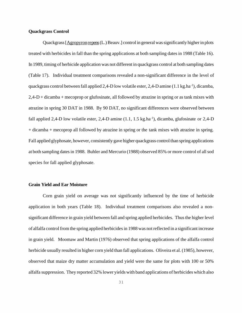
Quackgrass Control
Quackgrass [Agropyron repens (L.) Beauv.] control in general was significantly higher in plots
treated with herbicides in fall than the spring applications at both sampling dates in 1988 (Table 16).
In 1989, timing of herbicide application was not different in quackgrass control at both sampling dates
(Table 17). Individual treatment comparisons revealed a non-significant difference in the level of
quackgrass control between fall applied 2,4-D low volatile ester, 2,4-D amine (1.1 kg.ha-1), dicamba,
2,4-D + dicamba + mecoprop or glufosinate, all followed by atrazine in spring or as tank mixes with
atrazine in spring 30 DAT in 1988. By 90 DAT, no significant differences were observed between
fall applied 2,4-D low volatile ester, 2,4-D amine (1.1, 1.5 kg.ha-1), dicamba, glufosinate or 2,4-D
+ dicamba + mecoprop all followed by atrazine in spring or the tank mixes with atrazine in spring.
Fall applied glyphosate, however, consistently gave higher quackgrass control than spring applications
at both sampling dates in 1988. Buhler and Mercurio (1988) observed 85% or more control of all sod
species for fall applied glyphosate.
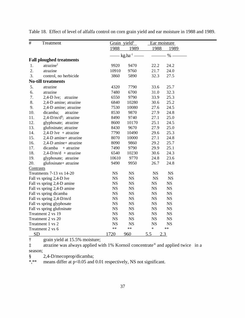
Grain Yield and Ear Moisture
Corn grain yield on average was not significantly influenced by the time of herbicide
application in both years (Table 18). Individual treatment comparisons also revealed a non-
significant difference in grain yield between fall and spring applied herbicides. Thus the higher level
of alfalfa control from the spring applied herbicides in 1988 was not reflected in a significant increase
in grain yield. Moomaw and Martin (1976) observed that spring applications of the alfalfa control
herbicide usually resulted in higher corn yield than fall applications. Oliveira et al. (1985), however,
observed that maize dry matter accumulation and yield were the same for plots with 100 or 50%
alfalfa suppression. They reported 32% lower yields with band applications of herbicides which also

32
achieved 50% alfalfa suppression. Grain yield was however significantly higher with conventional
tillage plus fall and spring postemergence atrazine relative to no-till with atrazine applied at the same
time. This result indicates that the application of atrazine alone may not be appropriate for alfalfa and
quackgrass control in no-till. Fall ploughing without any herbicide application (control) resulted in
the lowest grain yield of 3860 and 5890 kg.ha-1 in 1988 and 1989, respectively. The non-significant
difference in grain yield between the best no-till and ploughed plots is consistent with results obtained
in rotation studies in Ontario. Vyn (1987) observed that corn grain yields were lower (but usually non
significant) with no-till than with conventional tillage when corn was grown in rotation with crops
other than corn. The results are also in consonance with reports of Mock and Erbach (1977) and Levin
et al. (1987) who observed that grain yields with zero tillage have generally equalled or exceeded
those obtained with conventional tillage.
Ear moisture content at harvest was not significantly influenced by the time of herbicide
application for the individual treatment comparisons (Table 18). There was also no significant effect
of the levels of alfalfa and quackgrass control on the ear moisture at harvest. There was, however,
lower ear moisture for no-till corn compared to conventionally tilled corn where atrazine was applied
in fall and postemergence in spring (Table 18). This may be due poorer alfalfa control, hence
competition between corn and alfalfa within a no-till system.
33
CONCLUSIONS
Glufosinate applied in fall, plus atrazine in spring or as a tank mix with atrazine was most
consistent in controlling alfalfa and quackgrass with no difference between fall or spring applications.
Alfalfa and quackgrass control with glyphosate, 2,4-D amine or low volatile ester, dicamba or 2,4-D
+ dicamba + mecoprop varied with time of application over the two years of the research. Grain yield
and corn growth parameters were not influenced by time of herbicide application. Grain yields from
the best no-till plots were not significantly different from those obtained with conventional tillage.

34
Table 15. List of herbicide treatments applied for control of established alfalfa in no-till corn in1988 and 1989
Treatment Herbicide Dose Time of
# kg a.i. ha-1 Application
Fall ploughed treatments
1. atrazine† 2.0; 2.0 S ppi; post
2. atrazine 2.0; 2.0 F; post 3. control, no herbicide
No-till treatments 4. control, no herbicide 5. atrazine; 2.0; 2.0 S pre; post
6. atrazine; 2.0; 2.0 F; post 7. 2,4-D lve; atrazine 1.1; 2.0; 2.0 F; S pre; post
8. 2,4-D amine; atrazine 1.1; 2.0; 2.0 F; S pre; post 9. 2,4-D amine; atrazine 1.5; 2.0; 2.0 F; S pre; post
10. dicamba; atrazine 0.6; 2.0; 2.0 F; S pre; post11. 2,4-D/m/d‡; atrazine 1.1; 2.0; 2.0 F; S pre; post
12. glyphosate; atrazine 1.5; 2.0; 2.0 F; S pre; post13. glufosinate; atrazine 1.5; 2.0; 2.0 F; S pre; post
14. 2,4-D lve + atrazine 1.1+ 2.0; 2.0 S pre; post15. 2,4-D amine+ atrazine 1.1+ 2.0; 2.0 S pre; post
16. 2,4-D amine+ atrazine 1.5+ 2.0; 2.0 S pre; post17. dicamba + atrazine 0.6+ 2.0; 2.0 S pre; post
18. 2,4-D/m/d + atrazine 1.1+ 2.0; 2.0 S pre; post19. glyphosate; atrazine 1.5; 2.0; 2.0 S pre; post
20. glufosinate+ atrazine 1.5+ 2.0; 2.0 S pre; post
† atrazine was always applied with 1% Kornoil concentrate® and applied twice in a season; ‡ 2,4-D/mecoprop/dicamba;
F= fall applied prior to ploughing; S pre, S post = spring pre and postemergence respectively;lve= low volatile ester.

35
Table 16. Mean biomass values for alfalfa and quackgrass control in no-till corn in 1988.______________________________________________________________________________# Treatment ALF QGS ALF QGS --- 30 DAT† -- ---- 90 DAT ---
_________________ g m-2 __________________Fall ploughed treatments 1. atrazine‡ 2.3 8.1 3.1 84.5 2. atrazine 5.8 2.2 18.9 6.5 3. control, no herbicide 1.6 22.9 35.6 181.1No-till treatments 5. atrazine 40.3 41.6 28.9 64.1 6. atrazine 46.0 5.9 19.7 0.7 7. 2,4-D lve; atrazine 46.1 34.5 36.6 10.9 8. 2,4-D amine; atrazine 28.6 41.4 20.5 16.3 9. 2,4-D amine; atrazine 59.4 14.9 60.4 10.910. dicamba; atrazine 22.8 29.6 18.5 27.111. 2,4-D/m/d§; atrazine 39.1 35.6 49.9 21.612. glyphosate; atrazine 43.5 0.0 48.2 0.013. glufosinate; atrazine 61.5 2.1 39.9 3.014. 2,4-D lve + atrazine 2.4 40.7 11.8 11.315. 2,4-D amine+ atrazine 0.2 38.6 11.2 22.116. 2,4-D amine+ atrazine 3.4 50.4 16.9 20.117. dicamba + atrazine 0.1 45.6 2.8 36.918. 2,4-D/m/d + atrazine 0.0 60.3 5.9 18.819. glyphosate; atrazine 24.3 2.5 13.9 9.120. glufosinate+ atrazine 34.1 4.5 24.3 8.4ContrastsTreatments 7-13 vs 14-20 ** ** ** **Fall vs spring 2,4-D lve ** NS NS NSFall vs spring 2,4-D amine ** NS NS NSFall vs spring 2,4-D amine ** ** NS NSFall vs spring dicamba ** NS NS NSFall vs spring 2,4-D/m/d ** NS * NSFall vs spring glyphosate NS ** * *Fall vs spring glufosinate NS NS NS NS CV. % 65.6 58.5 106 133 SD 15.9 14.8 26.3 42.2
† days after spring preemergence herbicide application, 7.5, 9.5 months after fall herbicideapplication;
‡ atrazine was always applied with 1% Kornoil concentrate® and applied twice in a season; § 2,4-D/mecoprop/dicamba;ALF= alfalfa, QGS= quackgrass, lve= low volatile ester;*,** means differ at p<0.05 and 0.01 respectively, NS not significant

36
Table 17. Mean biomass values for alfalfa and quackgrass control in no-till corn in 1989.
-----30 DAT†--- ------90 DAT---- Treatment ALF QGS ALF QGS Fall ploughed treatments _________________ g m-2 ______________
1. atrazine‡ 1.0 3.7 0.0 6.2 2. atrazine 1.0 2.8 0.0 4.1 3. control, no herbicide 0.7 3.4 0.0 169.7 No-till treatments 5. atrazine 64.7 27.6 1.9 7.9 6. atrazine 83.1 84.1 5.9 32.0 7. 2,4-D lve; atrazine 12.1 33.5 0.6 5.7 8. 2,4-D amine; atrazine 9.2 29.4 0.0 1.1 9. 2,4-D amine; atrazine 8.4 36.7 0.0 11.210. dicamba; atrazine 1.8 31.2 3.9 1.411. 2,4-D/m/d§; atrazine 1.2 35.1 0.0 3.912. glyphosate; atrazine 2.3 0.1 1.4 0.8 13. glufosinate; atrazine 76.7 14.1 0.7 1.914. 2,4-D lve + atrazine 11.3 44.5 0.2 6.4 15. 2,4-D amine+ atrazine 11.0 47.1 5.4 0.916. 2,4-D amine+ atrazine 5.1 54.4 2.3 4.9 17. dicamba + atrazine 0.6 51.1 8.6 22.018. 2,4-D/m/d + atrazine 1.2 44.4 18.6 5.319. glyphosate; atrazine 47.2 0.1 0.0 6.820. glufosinate+ atrazine 74.5 10.2 4.7 2.6ContrastsTreatments 7-13 vs 14-20 ** NS ** NSFall vs spring 2,4-D lve NS NS NS NSFall vs spring 2,4-D amine NS NS NS NSFall vs spring 2,4-D amine NS NS NS NSFall vs spring dicamba NS NS NS NSFall vs spring 2,4-D/m/d NS NS ** NSFall vs spring glyphosate ** NS NS NSFall vs spring glufosinate NS NS NS NS CV % 79.4 40 223 128 SD 17.3 11.8 6.4 19.9 † days after spring preemergence herbicide application, 7.5, 9.5 months after fall herbicide
application;‡ atrazine was always applied with 1% Kornoil concentrate® and applied twice in a season; § 2,4-D/mecoprop/dicamba;ALF= alfalfa, QGS= quackgrass, lve= low volatile ester;*,** means differ at p<0.05 and 0.01 respectively, NS not significant.
37
Table 18. Effect of level of alfalfa control on corn grain yield and ear moisture in 1988 and 1989.
# Treatment Grain yield |+ Ear moisture 1988 1989 1988 1989 ____ kg.ha-1 ____ ______ % ______
Fall ploughed treatments 1. atrazine‡ 9920 9470 22.2 24.2 2. atrazine 10910 9760 21.7 24.0 3. control, no herbicide 3860 5890 32.3 27.5No-till treatments 5. atrazine 4320 7790 33.6 25.7 6. atrazine 7480 6700 31.0 32.3 7. 2,4-D lve; atrazine 6550 9790 33.9 25.3 8. 2,4-D amine; atrazine 6840 10280 30.6 25.2 9. 2,4-D amine; atrazine 7530 10080 27.6 24.510. dicamba; atrazine 8530 9870 27.9 24.811. 2,4-D/m/d§; atrazine 8490 9740 27.1 25.012. glyphosate; atrazine 8600 10170 25.1 24.513. glufosinate; atrazine 8430 9670 27.9 25.014. 2,4-D lve + atrazine 7790 10490 29.6 25.315. 2,4-D amine+ atrazine 8070 10000 27.1 24.816. 2,4-D amine+ atrazine 8090 9860 29.2 25.717. dicamba + atrazine 7490 9790 29.9 25.118. 2,4-D/m/d + atrazine 6540 10230 30.6 24.319. glyphosate; atrazine 10610 9770 24.8 23.620. glufosinate+ atrazine 9490 9950 26.7 24.8ContrastsTreatments 7-13 vs 14-20 NS NS NS NSFall vs spring 2,4-D lve NS NS NS NSFall vs spring 2,4-D amine NS NS NS NSFall vs spring 2,4-D amine NS NS NS NSFall vs spring dicamba NS NS NS NSFall vs spring 2,4-D/m/d NS NS NS NSFall vs spring glyphosate NS NS NS NSFall vs spring glufosinate NS NS NS NSTreatment 2 vs 19 NS NS NS NSTreatment 2 vs 20 NS NS NS NSTreatment 1 vs 2 NS NS NS NSTreatment 2 vs 6 ** ** * ** SD 1720 960 5.5 2.3 † grain yield at 15.5% moisture; ‡ atrazine was always applied with 1% Kornoil concentrate® and applied twice in aseason; § 2,4-D/mecoprop/dicamba;*,** means differ at p<0.05 and 0.01 respectively, NS not significant.

38
3.7 RECOMMENDATIONS
On the basis of field experiments conducted at different sites from 1987 to 1990 the
following recommendations are suggested for burndown of cover crops in no-till crop production
systems:
3.7.1 SOYBEANS
3.7.1.1 Alfalfa burndown
! Spring applied tank-mixture of glyphosate at 0.90 kg.ha-1 + 2,4-D (amine or ester) at 1.0
kg.ha-1 can provide excellent established alfalfa control. The dandelion may be more
efficiently controlled by the ester formulation of 2,4-D.
3.7.1.2 Winter wheat
! For control of winter wheat, apply glyphosate at 0.45 to 0.90 kg.ha-1 or paraquat at 1.0
kg.ha-1 to wheat seedlings up to 4 leaf stage of growth.
3.7.2 WINTER WHEAT BURNDOWN WITH GLYPHOSATE
! Winter wheat burndown was found to be dependent upon the growth stage of wheat at the
time of herbicide application, herbicide dose and additives.

39
! Apply glyphosate at 0.30 kg.ha-1 + ammonium sulphate at 2 l.ha-1 + Agral® 90 at 0.1% (v/v)
to winter wheat seedlings in 2 to 3 leaf (12-14 cm tall) stage of the growth.
! Apply glyphosate at 0.45 kg.ha-1 + ammonium sulphate at 2 l.ha-1 + Agral® 90 at 0.1% (v/v)
to winter wheat seedlings in 3 to 4 leaf (12-14 cm tall) stage of the growth.
! Apply glyphosate at 0.60 kg.ha-1 + ammonium sulphate at 2 l.ha-1 + Agral® 90 at 0.1% (v/v)
or glyphosate alone at 0.90 kg.ha-1 to winter wheat seedlings in 4 to 5 leaf (12-14 cm tall)
stage of the growth.
3.7.3 CORN
3.7.3.1 Red Clover Burndown
The following herbicides are recommended for established red clover burndown in corn.
These herbicides should be tank-mixed with 1% (v/v) Kornoil concentrate®.
! 2,4-D (ester or amine) at 0.50 to 1.0 kg.ha-1 + atrazine at 1.50 kg.ha-1 + metolachlor at 1.92
kg.ha-1 before the emergence of corn.
! Glufosinate at 1.0 kg.ha-1 + metolachlor at 1.68 kg.ha-1 + atrazine at 1.50 kg.ha-1 or dicamba
at 0.60 kg.ha-1 applied preemergence to corn.
! Paraquat at 1.0 kg.ha-1 + metolachlor at 1.68 kg.ha-1 + atrazine at 1.50 kg.ha-1 or dicamba at
0.60 kg.ha-1 applied preemergence to corn.
! Dicamba at 0.60 kg.ha-1 + atrazine at 1.50 kg.ha-1 + metolachlor at 1.92 kg.ha-1
preemergence to corn.

40
! Glyphosate at 0.90 kg.ha-1 followed by metolachlor at 1.68 kg.ha-1 + atrazine at 1.50 kg.ha-1
or dicamba at 0.60 kg.ha-1.
Precaution: Glyphosate was applied as pre-split with metolachlor + atrazine or dicamba.
3.7.3.2 Alfalfa burndown
! Apply glyphosate at 1.5 kg.ha-1 in the fall followed by a spring application of atrazine at
2.0 kg.ha-1.
! Apply atrazine at 2.0 kg.ha-1 in the fall and again at 2.0 kg.ha-1 the following spring.
! Dicamba at 0.6 kg.ha-1 + atrazine at 2.0 kg.ha-1 applied in the spring prior to the corn
planting.
! 2,4-D/mecoprop/dicamba at 1.1 kg.ha-1 + atrazine at 2.0 kg.ha-1 applied in the spring prior
to the corn planting.
! Glufosinate at 1.5 kg.ha-1 in the fall followed by a spring application of atrazine at 2.0
kg.ha-1 or as a tank-mix of glufosinate + atrazine applied in the spring prior to corn
planting.
41
OBJECTIVE # 2
4.0 ANTAGONISM OF BURNDOWN HERBICIDES WITH RESIDUAL HERBICIDESIN CONSERVATION TILLAGE SYSTEMS
Weed population dynamics may be altered by the elimination of tillage. The weed flora in
a no-till cropping system is often more diverse than in a conventional tillage system. The
successful establishment of the crop is very dependent upon herbicides for the control of weeds.
The majority of recommended herbicides control only a limited spectrum of weeds.
Therefore, to manage a diverse weed flora, various herbicide combinations may be required. The
ability to safely tank-mix herbicides can reduce trips across the field, ultimately saving money and
fuel for the farmers. However, not all of the herbicides can be tank-mixed. Herbicides usually
have chemical and physical properties which, upon mixing, may affect herbicidal activity.
To overcome these challenges a series of field experiments were initiated in Ontario with
tank-mixes of various burndown and residual herbicides. The objective of these experiments was
to study the interaction of tank-mixing various burndown herbicides with residual preemergence
herbicides for annual weed control in corn and soybeans in various conservative tillage systems.

42
4.1 METHODS AND MATERIALS
Field experiments were conducted to evaluate the effect of the tank-mixing of burndown
and residual herbicides on weed control in no-till systems. The details of experimental
procedures followed and material used are described briefly.
4.1.1 Experimental Locations
Details of experimental locations and soil types are described in Table 19.
Table 19. Details of experiment locations and soil types for experiments conducted from
1987 to 1990.
______________________________________________________________________________
Crop Experiment Soil # Site Location Type Sand Silt Clay O.M. pH______________________________________________________________________________
_________ % ________
Corn 4.2† Dealtown 42E 15'N Fox Gravelly 59 31 10 2.8 6.182E 5 'W Loam
Corn 4.3† Dealtown 42E 15'N Fox Gravelly 59 31 10 2.8 6.1 82E 5 'W Loam
Soybeans 4.4† Dealtown 42E 15'N Fox Gravelly 59 31 10 2.8 6.182E 5 'W Loam
Soybeans 4.5 Dealtown 42E 15'N Fox Gravelly 59 31 10 2.8 6.182E 5 'W Loam
Fallow/ 4.6 Elora 42E 27'N Guelph Loam 29 53 18 4.3 7.5Quackgrass 81E 53'W______________________________________________________________________________|+ Experiment was conducted at Mr. Art Wardle's farm, Ridgetown, Ontario on Brookston
clay loam soil in 1987.

43
4.1.2 Agronomy
Experiments were conducted using standard agronomic practices (OMAF publication 296,
Field Crop Recommendations) in no-till plots. Soil samples were taken from each field at the
beginning of the crop season and were analyzed for soil available nutrient status. Fertilization was
done according to soil tests and requirements of individual crop. Fertilizer was placed at the time
of sowing of the crop with minimum soil surface disturbances.
Corn cv. Renk® R148, Dekalb® 524, Renk® R138, Pioneer® 3790 were planted at their
respective recommended seeding densities in 76 cm rows in 1987, 1988, 1989 and 1990,
respectively. The individual corn plot size was 6 x 1.5 m.
Soybeans cv. Hodgson and Elgin were planted at a seeding rate of 80 kg/ha in 38 cm rows
in 1987 and 1988, 1989, 1990; respectively. The individual soybeans plot size was 6 x 1.5 m.
The quackgrass experiment was established using the quackgrass biotype found at Elora
Research Station, Elora, Ontario. The individual size of quackgrass plots was 6 x 2 m.
Corn and soybeans were harvested from the centre of plots leaving side border rows at
Elora site and from whole plot at Dealtown site. Final yield was later converted and expressed at
14% and 15.5% moisture content for soybeans and corn, respectively.
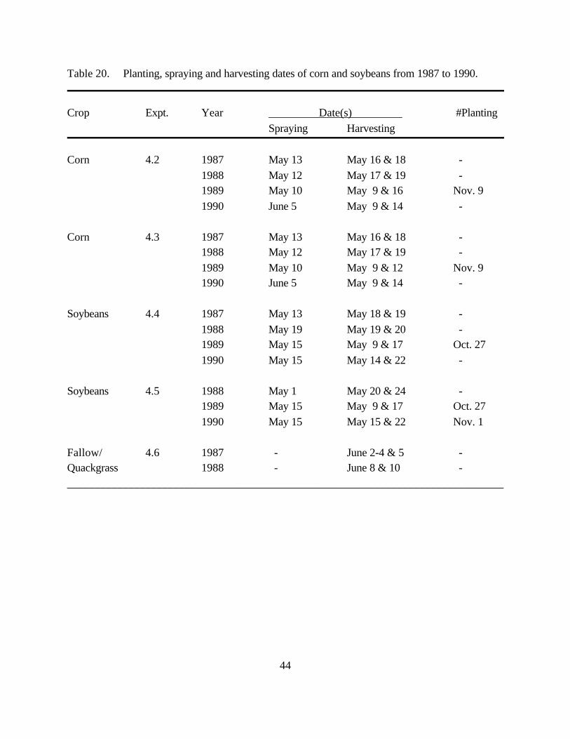
The details of dates of planting, spraying and crop harvesting are presented in Table 20.
44
Table 20. Planting, spraying and harvesting dates of corn and soybeans from 1987 to 1990.
Crop Expt. Year Date(s) #Planting
Spraying Harvesting
Corn 4.2 1987 May 13 May 16 & 18 -
1988 May 12 May 17 & 19 -1989 May 10 May 9 & 16 Nov. 9
1990 June 5 May 9 & 14 -
Corn 4.3 1987 May 13 May 16 & 18 -1988 May 12 May 17 & 19 -
1989 May 10 May 9 & 12 Nov. 91990 June 5 May 9 & 14 -
Soybeans 4.4 1987 May 13 May 18 & 19 -
1988 May 19 May 19 & 20 -1989 May 15 May 9 & 17 Oct. 27
1990 May 15 May 14 & 22 -
Soybeans 4.5 1988 May 1 May 20 & 24 -1989 May 15 May 9 & 17 Oct. 27
1990 May 15 May 15 & 22 Nov. 1
Fallow/ 4.6 1987 - June 2-4 & 5 -Quackgrass 1988 - June 8 & 10 -
______________________________________________________________________________

45
4.1.3 Spraying Equipment and Procedures
Individual plots were sprayed using a 'bicycle sprayer' at Elora site and by an 'Oxford
Precision Sprayer' at Dealtown site. The quantity of spray solution used for the bicycle sprayer
was 225 l.ha-1 at 180 kPa. The 'Oxford Precision Sprayer' used 200 l.ha-1 of spray solution at 240
kPa.
4.1.4 Experiment Design and Analysis
All experiments were conducted in randomized complete block design (RCBD) with 4
replications. Results were analyzed using analysis of variance (ANOVA) procedures and means
were then separated using least significant difference (LSD) at 5% level of significance.

46
4.2 PARAQUAT AND GLUFOSINATE ANTAGONISM WITH RESIDUALHERBICIDES IN NO-TILL CORN
RESEARCH SUMMARY:
Excellent weed burndown was achieved with paraquat, glufosinate and metolachlor +
atrazine or cyanazine + additives. However, the tank-mix of paraquat plus dicamba or atrazine
(liquid formulation) failed to burndown weeds in 1990.
Residual broadleaf weed control by various herbicide combinations was excellent in 1989
and 1990. Weather in 1987 and 1988 was very dry in the beginning of the season and thus some
herbicide combinations failed to provide satisfactory broadleaf weed-control. Atrazine provided
excellent broadleaf weed control in these dry years except when it was applied with metolachlor
in the absence of burndown herbicides. Cyanazine when tank-mixed with other herbicides also
failed to provide satisfactory weed control in 1987 and 1988.
Annual grass control by various herbicides was excellent in 1989 and 1990. All herbicide
combinations gave poor to very poor grass control in 1987. However, the grass control was
satisfactory to excellent in 1988 except when metolachlor + cyanazine + oil failed to provide grass
control.
Corn yields were similar whether paraquat was applied separately or tank-mixed with
residual herbicides. However, among separately applied residual herbicides with paraquat, corn
yields were significantly less in metribuzin treated plots as compared to atrazine treated plots.
Similarly, among tank-mixed residual and paraquat treatments, atrazine (WG) treated plots had
significantly higher corn yields as compared to metribuzin or dicamba treated plots.

47
Among glufosinate treated plots, atrazine when tank-mixed with the higher dosage of
glufosinate resulted in significantly less corn yields than the identical treatment applied at the
lower glufosinate dosage. Corn yields resulting from atrazine or cyanazine with additives were
not affected due to the absence of burndown herbicides.
Table 21. Corn yield as affected by various treatments in 1989.
# Treatment+| Dose Yield
kg a.i./ha
____ kg/ha _____ 1 Paraquat; metolachlor + atrazine (WG)‡ 0.5; 2.4 + 1.5 7780
2 Paraquat; metolachlor + cyanazine (WP) 0.5; 2.4 + 2.0 6710 3 Paraquat; metolachlor + dicamba 0.5; 2.4 + 0.6 5860
4 Paraquat; metolachlor + metribuzin (DF) 0.5; 2.4 + .75 5200 5 Paraquat + metolachlor + atrazine (WG) 0.5 + 2.4 + 1.5 8820
6 Paraquat + metolachlor + atrazine (L) 0.5 + 2.4 + 1.5 7190 7 Paraquat + metolachlor + cyanazine (WP) 0.5 + 2.4 + 2.0 8210
8 Paraquat + metolachlor + cyanazine (L) 0.5 + 2.4 + 2.0 6700 9 Paraquat + metolachlor + dicamba 0.5 + 2.4 + 0.6 6500
10 Paraquat + metolachlor + metribuzin (DF) 0.5 + 2.4 + 0.75 448011 Paraquat + metolachlor + metribuzin (L) 0.5 + 2.4 + 0.75 3560
12 Glufosinate; metolachlor + atrazine (WG) 0.5 + 2.4 + 1.5 789013 Glufosinate; metolachlor + atrazine (WG) 0.75+ 2.4 + 1.5 8660
14 Glufosinate + metolachlor + atrazine (WG) 0.5 + 2.4 + 1.5 568015 Glufosinate + metolachlor + atrazine (WG) 0.75+ 2.4 + 1.5 8420
16 Metolachlor + atrazine + oil 2.4 + 1.5 + 10 L 710017 Metolachlor + atrazine + oil conc. 2.4 + 1.5 + 2 L 7720
18 Metolachlor + cyanazine + oil 2.4 + 2.25 + 10 L 725019 Metolachlor + cyanazine + oil conc. 2.4 + 2.25 + 2 L 7800
20 Weedy check 2520LSD 5% 2130
+| in treatments 1 to 4, 11 and 12 residual and burndown herbicides were applied separately.In the rest of the treatments herbicides were tank-mixed at time of herbicide application.
‡ WG= wettable granules, WP= wettable powder, DF= dry flowable, L= liquid
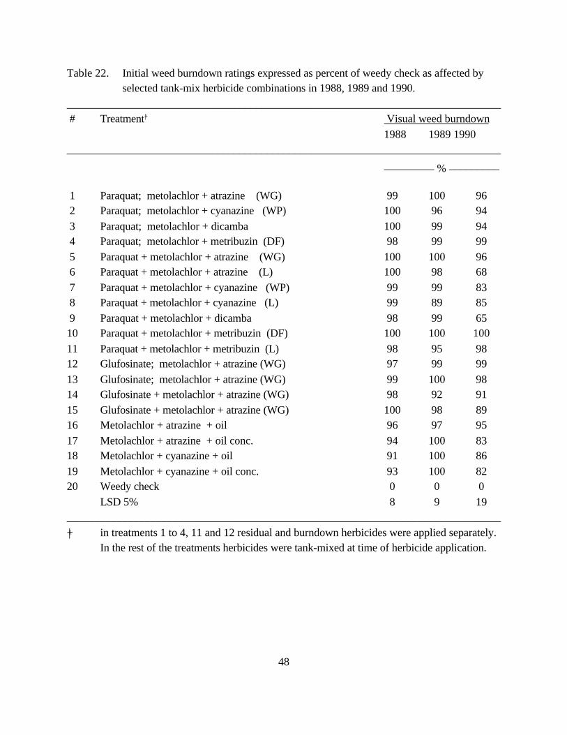
48
Table 22. Initial weed burndown ratings expressed as percent of weedy check as affected byselected tank-mix herbicide combinations in 1988, 1989 and 1990.
______________________________________________________________________________ # Treatment+| Visual weed burndown
1988 1989 1990______________________________________________________________________________
_________ % _________
1 Paraquat; metolachlor + atrazine (WG) 99 100 96 2 Paraquat; metolachlor + cyanazine (WP) 100 96 94
3 Paraquat; metolachlor + dicamba 100 99 94 4 Paraquat; metolachlor + metribuzin (DF) 98 99 99
5 Paraquat + metolachlor + atrazine (WG) 100 100 96 6 Paraquat + metolachlor + atrazine (L) 100 98 68
7 Paraquat + metolachlor + cyanazine (WP) 99 99 83 8 Paraquat + metolachlor + cyanazine (L) 99 89 85
9 Paraquat + metolachlor + dicamba 98 99 6510 Paraquat + metolachlor + metribuzin (DF) 100 100 100
11 Paraquat + metolachlor + metribuzin (L) 98 95 9812 Glufosinate; metolachlor + atrazine (WG) 97 99 99
13 Glufosinate; metolachlor + atrazine (WG) 99 100 9814 Glufosinate + metolachlor + atrazine (WG) 98 92 91
15 Glufosinate + metolachlor + atrazine (WG) 100 98 8916 Metolachlor + atrazine + oil 96 97 95
17 Metolachlor + atrazine + oil conc. 94 100 8318 Metolachlor + cyanazine + oil 91 100 86
19 Metolachlor + cyanazine + oil conc. 93 100 8220 Weedy check 0 0 0
LSD 5% 8 9 19______________________________________________________________________________
+| in treatments 1 to 4, 11 and 12 residual and burndown herbicides were applied separately.In the rest of the treatments herbicides were tank-mixed at time of herbicide application.

49
Table 23. Annual broadleaf weed control ratings expressed as percent of weedy check asaffected by selected tank-mix herbicide combinations in 1987, 1988, 1989 and 1990.
______________________________________________________________________________ # Treatment+| Broadleaf visual control
1987 1988 1989 1990______________________________________________________________________________
___________ % __________
1 Paraquat; metolachlor + atrazine (WG) 89 80 100 85 2 Paraquat; metolachlor + cyanazine (WP) 89 84 100 89
3 Paraquat; metolachlor + dicamba 88 83 100 88 4 Paraquat; metolachlor + metribuzin (DF) 65 75 100 96
5 Paraquat + metolachlor + atrazine (WG) 90 85 100 95 6 Paraquat + metolachlor + atrazine (L) 84 71 99 68
7 Paraquat + metolachlor + cyanazine (WP) 83 55 100 85 8 Paraquat + metolachlor + cyanazine (L) 64 48 100 83
9 Paraquat + metolachlor + dicamba 81 80 99 6410 Paraquat + metolachlor + metribuzin (DF) 76 79 100 98
11 Paraquat + metolachlor + metribuzin (L) 89 81 100 9812 Glufosinate; metolachlor + atrazine (WG) 86 78 100 99
13 Glufosinate; metolachlor + atrazine (WG) 84 81 100 9914 Glufosinate + metolachlor + atrazine (WG) 90 83 91 93
15 Glufosinate + metolachlor + atrazine (WG) 88 76 98 9216 Metolachlor + atrazine + oil 64 74 97 96
17 Metolachlor + atrazine + oil conc. 31 75 100 9118 Metolachlor + cyanazine + oil 85 48 100 81
19 Metolachlor + cyanazine + oil conc. 65 60 97 8820 Weedy check 0 0 0 0
LSD 5% 30 17 5 15______________________________________________________________________________
+| in treatments 1 to 4, 11 and 12 residual and burndown herbicides were applied separately.In the rest of the treatments herbicides were tank-mixed at time of herbicide application.

50
Table 24. Annual grass weed control ratings expressed as percent of weedy check as affectedby selected tank-mix herbicide combinations in 1987, 1988, 1989 and 1990.
______________________________________________________________________________ # Treatment+| Annual grass control
1987 1988 1989 1990______________________________________________________________________________
___________ % __________ 1 Paraquat; metolachlor + atrazine (WG) 43 88 100 100
2 Paraquat; metolachlor + cyanazine (WP) 30 86 95 100 3 Paraquat; metolachlor + dicamba 18 90 99 100
4 Paraquat; metolachlor + metribuzin (DF) 40 83 95 100 5 Paraquat + metolachlor + atrazine (WG) 50 81 100 100
6 Paraquat + metolachlor + atrazine (L) 41 88 99 100 7 Paraquat + metolachlor + cyanazine (WP) 40 75 99 100
8 Paraquat + metolachlor + cyanazine (L) 51 78 100 100 9 Paraquat + metolachlor + dicamba 36 85 100 100
10 Paraquat + metolachlor + metribuzin (DF) 33 80 100 10011 Paraquat + metolachlor + metribuzin (L) 28 76 100 100
12 Glufosinate; metolachlor + atrazine (WG) 28 80 100 10013 Glufosinate; metolachlor + atrazine (WG) 28 88 100 100
14 Glufosinate + metolachlor + atrazine (WG) 53 79 100 10015 Glufosinate + metolachlor + atrazine (WG) 0 80 100 100
16 Metolachlor + atrazine + oil 35 78 100 10017 Metolachlor + atrazine + oil conc. 39 88 100 100
18 Metolachlor + cyanazine + oil 13 69 100 10019 Metolachlor + cyanazine + oil conc. 41 85 100 100
20 Weedy check 0 0 0 0LSD 5% NS 14 4 0.3
______________________________________________________________________________+| in treatments 1 to 4, 11 and 12 residual and burndown herbicides were applied separately.
In the rest of the treatments herbicides were tank-mixed at time of herbicide application.

51
4.3 GLYPHOSATE ANTAGONISM WITH RESIDUAL HERBICIDES IN NO-TILL
CORN
RESEARCH SUMMARY:
Glyphosate was applied at four application rates: 0.30, 0.45, 0.68 and 0.90 kg/ha, to
evaluate the potential for antagonism when tank-mixed with atrazine or cyanazine. Atrazine and
cyanazine wettable granules (WG) or liquid (L) formulations were tank-mixed with glyphosate.
Glyphosate was always applied with ammonium sulphate and Agral® 90 additives. Residual
herbicide metolachlor at 2.4 kg.ha-1 was applied with every herbicide treatments.
Burndown of annual weeds was not affected at any tested glyphosate application rates
and/or tank-mixing of atrazine or cyanazine in any tested formulations. However, when dicamba
replaced atrazine or cyanazine as the residual herbicide with glyphosate, a significant reduction in
weed burndown occurred, compared to atrazine or cyanazine with glyphosate.
Annual broadleaf weed control by various treatments was generally fair to excellent.
However, there were few exceptions. Tank-mixed atrazine (L) with a high dose of glyphosate
(0.90 kg.ha-1) provided significantly less broadleaf weed control than atrazine (WG) + glyphosate
in 1987 or as a split application of atrazine (WG) + glyphosate in 1988. Dicamba treated plots
also had significantly less broadleaf weed control than atrazine or cyanazine treated plots.
Annual grass control in 1989, 1990 was better than 1987, 1988. Weather in first two years
was extremely dry and thus may have affected herbicidal activity. Tank-mixed atrazine gave poor
grass control as compared to the split application. Cyanazine when tank-mixed with lower doses
of glyphosate failed to control annual grasses in 1987.

52
Corn yields were significantly reduced in plots treated with dicamba. Glyphosate at
high application rates consistently provided higher corn yields and its performance was similar
whether it was applied with residual herbicides in split application or was tank-mixed.
Table 25. Corn yield as affected by various treatments in 1989.
______________________________________________________________________________ # Treatment|+ Dose Yield
kg a.i./ha 1989
_ kg/ha _
1 Weedy check 1460
2 Glyphosate |=; metolachlor + atrazine (WP) .30; 2.4 + 1.5 5660
3 Glyphosate; metolachlor + atrazine (WP) .45; 2.4 + 1.5 4180
4 Glyphosate; metolachlor + atrazine (WP) .68; 2.4 + 1.5 5290
5 Glyphosate; metolachlor + atrazine (WP) .90; 2.4 + 1.5 6670
6 Glyphosate + metolachlor + atrazine (WP) .30 + 2.4 + 1.5 5840
7 Glyphosate + metolachlor + atrazine (WP) .45 + 2.4 + 1.5 6750
8 Glyphosate + metolachlor + atrazine (WP) .68 + 2.4 + 1.5 6870
9 Glyphosate + metolachlor + atrazine (WP) .90 + 2.4 + 1.5 7030
10 Glyphosate + metolachlor + atrazine (L) .30 + 2.4 + 1.5 6890
11 Glyphosate + metolachlor + atrazine (L) .45 + 2.4 + 1.5 6470
12 Glyphosate + metolachlor + atrazine (L) .68 + 2.4 + 1.5 6130
13 Glyphosate + metolachlor + atrazine (L) .90 + 2.4 + 1.5 6070
14 Glyphosate; metolachlor + cyanazine (WP) .45; 2.4 + 2.0 6810
15 Glyphosate; metolachlor + cyanazine (WP) .90; 2.4 + 2.0 5850
16 Glyphosate + metolachlor + cyanazine (WP) .45 + 2.4 + 2.0 4490
17 Glyphosate + metolachlor + cyanazine (WP) .90 + 2.4 + 2.0 5800
18 Glyphosate + metolachlor + cyanazine (L) .45 + 2.4 + 2.0 6330
19 Glyphosate + metolachlor + cyanazine (L) .90 + 2.4 + 2.0 6220
20 Glyphosate + metolachlor + dicamba .45 + 2.4 + 0.6 2790
LSD 2210
______________________________________________________________________________|+ treatments 2 to 5, 14 and 15 were applied in split. In other treatments herbicides were tank-
mixed at the time of application.|= Glyphosate was always applied with ammonium sulphate at 2 kg.ha-1 + Agral® 90 at 0.5%
(v/v).

53
Table 26. Initial weed burndown ratings expressed as percent of weedy check as affected bytank-mixing of glyphosate and additives with residual herbicides in 1988, 1989 and
1990.______________________________________________________________________________
# Treatment|+ Weed burndown ratings 1988 1989 1990
______________________________________________________________________________ ________ % ________
1 Weedy check 0 0 0
2 Glyphosate; metolachlor + atrazine (WP) 91 86 99 3 Glyphosate; metolachlor + atrazine (WP) 82 71 100
4 Glyphosate; metolachlor + atrazine (WP) 89 82 100 5 Glyphosate; metolachlor + atrazine (WP) 100 92 100
6 Glyphosate + metolachlor + atrazine (WP) 97 69 92 7 Glyphosate + metolachlor + atrazine (WP) 99 92 97
8 Glyphosate + metolachlor + atrazine (WP) 88 97 98 9 Glyphosate + metolachlor + atrazine (WP) 90 86 100
10 Glyphosate + metolachlor + atrazine (L) 94 96 9711 Glyphosate + metolachlor + atrazine (L) 97 89 96
12 Glyphosate + metolachlor + atrazine (L) 91 97 9813 Glyphosate + metolachlor + atrazine (L) 96 99 100
14 Glyphosate; metolachlor + cyanazine (WP) 78 100 9915 Glyphosate; metolachlor + cyanazine (WP) 79 93 100
16 Glyphosate + metolachlor + cyanazine (WP) 75 95 9717 Glyphosate + metolachlor + cyanazine (WP) 85 89 98
18 Glyphosate + metolachlor + cyanazine (L) 92 99 9319 Glyphosate + metolachlor + cyanazine (L) 85 94 98
20 Glyphosate + metolachlor + dicamba 88 51 70LSD 5% 15 27 22
______________________________________________________________________________|+ Glyphosate was always applied with ammonium sulphate at 2 kg.ha-1 + Agral® 90 at 0.5%
(v/v).

54
Table 27. Annual broadleaf weed control ratings expressed as percent of weedy check asaffected by tank-mixing glyphosate and additives with residual herbicides in 1987,
1988, 1989 and 1990.______________________________________________________________________________
# Treatment|+ Broadleaf weed control 1987 1988 1989 1990
__________________________________________________________________________________________ % _____________
1 Weedy check 0 0 0 0
2 Glyphosate; metolachlor + atrazine (WP) 84 80 99 97 3 Glyphosate; metolachlor + atrazine (WP) 79 79 100 98
4 Glyphosate; metolachlor + atrazine (WP) 86 85 100 98 5 Glyphosate; metolachlor + atrazine (WP) 85 88 100 98
6 Glyphosate + metolachlor + atrazine (WP) 76 75 97 95 7 Glyphosate + metolachlor + atrazine (WP) 75 75 92 96
8 Glyphosate + metolachlor + atrazine (WP) 83 73 97 99 9 Glyphosate + metolachlor + atrazine (WP) 81 75 98 99
10 Glyphosate + metolachlor + atrazine (L) 86 79 98 9811 Glyphosate + metolachlor + atrazine (L) 75 81 100 99
12 Glyphosate + metolachlor + atrazine (L) 84 83 100 10013 Glyphosate + metolachlor + atrazine (L) 16 66 99 100
14 Glyphosate; metolachlor + cyanazine (WP) 86 78 95 9015 Glyphosate; metolachlor + cyanazine (WP) 84 76 100 95
16 Glyphosate + metolachlor + cyanazine (WP) 80 71 91 9017 Glyphosate + metolachlor + cyanazine (WP) 80 61 93 88
18 Glyphosate + metolachlor + cyanazine (L) 81 65 95 8719 Glyphosate + metolachlor + cyanazine (L) 80 43 93 89
20 Glyphosate + metolachlor + dicamba 83 86 71 64LSD 12 18 12 19
______________________________________________________________________________|+ Glyphosate was always applied with ammonium sulphate at 2 kg.ha-1 + Agral® 90 at 0.5%
(v/v).

55
Table 28. Annual grass weed control ratings expressed as percent of weedy check as affected bytank-mixing glyphosate and additives with residual herbicides in 1987, 1988, 1989
and 1990.______________________________________________________________________________
# Treatment|+ Grass control ratings 1987 1988 1989 1990
__________________________________________________________________________________________ % ___________
1 Weedy check 0 0 0 0
2 Glyphosate; metolachlor + atrazine (WP) 54 85 100 100 3 Glyphosate; metolachlor + atrazine (WP) 28 85 100 100
4 Glyphosate; metolachlor + atrazine (WP) 74 85 99 99 5 Glyphosate; metolachlor + atrazine (WP) 76 90 99 100
6 Glyphosate + metolachlor + atrazine (WP) 39 75 99 100 7 Glyphosate + metolachlor + atrazine (WP) 58 77 99 100
8 Glyphosate + metolachlor + atrazine (WP) 40 71 100 100 9 Glyphosate + metolachlor + atrazine (WP) 51 76 100 100
10 Glyphosate + metolachlor + atrazine (L) 39 76 99 9911 Glyphosate + metolachlor + atrazine (L) 40 88 100 100
12 Glyphosate + metolachlor + atrazine (L) 36 78 99 10013 Glyphosate + metolachlor + atrazine (L) 55 88 100 100
14 Glyphosate; metolachlor + cyanazine (WP) 73 80 93 9915 Glyphosate; metolachlor + cyanazine (WP) 71 79 100 98
16 Glyphosate + metolachlor + cyanazine (WP) 0 70 100 10017 Glyphosate + metolachlor + cyanazine (WP) 74 75 99 100
18 Glyphosate + metolachlor + cyanazine (L) 50 81 98 9919 Glyphosate + metolachlor + cyanazine (L) 80 79 99 97
20 Glyphosate + metolachlor + dicamba 73 68 98 75LSD 41 13 3 23
______________________________________________________________________________|+ Glyphosate was always applied with ammonium sulphate at 2 kg.ha-1 + Agral® 90 at 0.5%
(v/v).

56
4.4 PARAQUAT AND GLUFOSINATE ANTAGONISM WITH RESIDUAL
HERBICIDES IN NO-TILL SOYBEANS
RESEARCH SUMMARY:
Excellent weed burndown was recorded with all herbicide treatments. However, paraquat
when tank-mixed with chloramben SG (soluble granules) provided significantly less weed
burndown as compared to tank-mixed paraquat with linuron or metribuzin in 1988 and with
paraquat + metribuzin in 1989. Similarly, a single application of linuron + oil failed to adequately
control weeds in 1990.
Residual herbicides provided excellent control of annual weeds in 1989 and 1990 but poor to
satisfactory annual weed control in 1987 and 1988. Weather in the first two years was very dry in
the beginning of crop season and thus resulted in erratic herbicidal activity. Residual herbicides,
chloramben and metolachlor/metobromuron when tank-mixed with paraquat resulted in poor
broadleaf weed control as compared to paraquat tank-mixed with linuron or metribuzin. Similarly,
tank-mixed paraquat + chloramben, or glufosinate + metribuzin + oil; separately applied paraquat
+ linuron or paraquat + chloramben failed to control annual grasses in different years.
Soybean yields were not affected due to reduction in glufosinate dosage or whether it was
tank-mixed with other residual herbicides. Paraquat treated plots generally had the same trend.
Tank-mixed paraquat with metribuzin (L) or linuron (WP) significantly reduced soybeans yields as
compared to a separate application of paraquat followed by either metribuzin (DF) or linuron
(WP) in 1990.

57
Table 29. Soybeans yield as affected by various treatments in 1989 and 1990.______________________________________________________________________________
# Treatment+| Dose Yield kg a.i./ha 1989 1990
________________________________________________________________________________ kg.ha-1 __
1 Paraquat; metola. |= + metri.§ (DF) 0.5; 2.4 + .56 3140 3490 2 Paraquat; metola. + linuron (WP) 0.5; 2.4 + 1 3520 3420
3 Paraquat; metola. + chloramben (SG) 0.5; 2.4 + 3 3400 2670 4 Paraquat; metola./metobromuron (EC) 0.5; 4.25 3460 2430
5 Paraquat + metola. + metri. (DF) 0.5 + 2.4 + .56 3030 3430 6 Paraquat + metola. + metri. (L) 0.5 + 2.4 + .56 3040 1870
7 Paraquat + metola. + linuron (WP) 0.5 + 2.4 + 1 2850 2080 8 Paraquat + metola. + linuron (L) 0.5 + 2.4 + 1 3100 2280
9 Paraquat + metola. + chloramben (SG) 0.5 + 2.4 + 3 2930 223010 Paraquat + metola. + metri. (DF) 1.0 + 2.4 + .56 3290 2660
11 Paraquat + metola./metobromuron (EC) 0.5 + 4.25 2970 269012 Glufosinate; metola. + metri. (DF) 0.5 + 2.4 + .56 3220 2920
13 Glufosinate; metola. + metri. (DF) 0.75 + 2.4 + .56 3340 240014 Glufosinate; metola. + metri. (DF) 0.5 + 2.4 + .56 3500 3330
15 Glufosinate + metola. + metri. (DF) 0.75 + 2.4 + .56 2950 307016 Glufosinate + metola. + metri. (L) 0.75 + 2.4 + .56 3320 2630
17 Glufosinate + metri. (DF) + oil 0.75 + 1 + 10 L 3300 292018 Glufosinate + metri. (DF) + oil conc. 0.75 + 1 + 2 L 4160 2690
19 Linuron + oil 2.0 + 10 L 2600 174020 Weedy check 1920 0820
LSD 5% 1080 1320______________________________________________________________________________
+| in treatments 1 to 4, 12 and 13 residual and burndown herbicides were applied separately.Remaining herbicide treatments were tank-mixed at the time of spray.
|= Metolachlor,§ Metribuzin
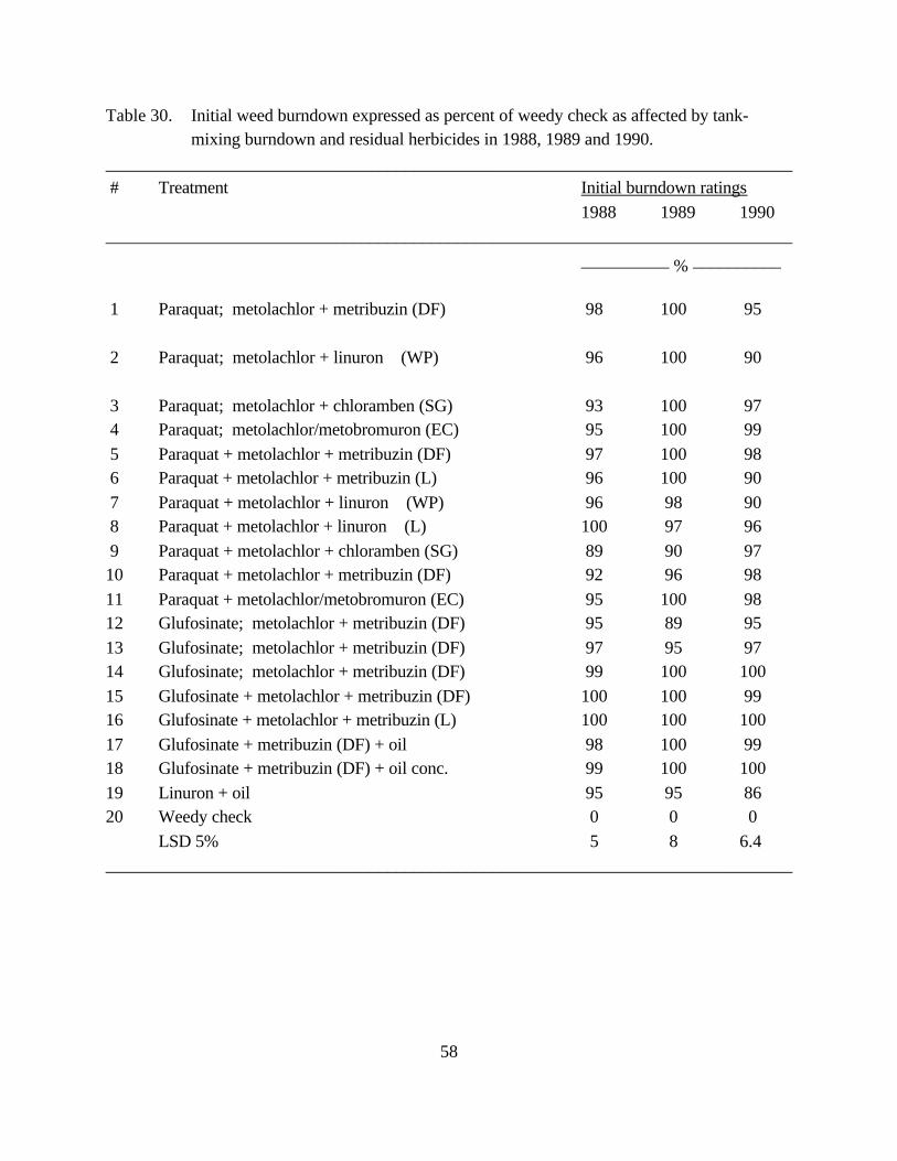
58
Table 30. Initial weed burndown expressed as percent of weedy check as affected by tank-mixing burndown and residual herbicides in 1988, 1989 and 1990.
______________________________________________________________________________ # Treatment Initial burndown ratings
1988 1989 1990______________________________________________________________________________
__________ % __________
1 Paraquat; metolachlor + metribuzin (DF) 98 100 95
2 Paraquat; metolachlor + linuron (WP) 96 100 90
3 Paraquat; metolachlor + chloramben (SG) 93 100 97 4 Paraquat; metolachlor/metobromuron (EC) 95 100 99
5 Paraquat + metolachlor + metribuzin (DF) 97 100 98 6 Paraquat + metolachlor + metribuzin (L) 96 100 90
7 Paraquat + metolachlor + linuron (WP) 96 98 90 8 Paraquat + metolachlor + linuron (L) 100 97 96
9 Paraquat + metolachlor + chloramben (SG) 89 90 9710 Paraquat + metolachlor + metribuzin (DF) 92 96 98
11 Paraquat + metolachlor/metobromuron (EC) 95 100 9812 Glufosinate; metolachlor + metribuzin (DF) 95 89 95
13 Glufosinate; metolachlor + metribuzin (DF) 97 95 9714 Glufosinate; metolachlor + metribuzin (DF) 99 100 100
15 Glufosinate + metolachlor + metribuzin (DF) 100 100 9916 Glufosinate + metolachlor + metribuzin (L) 100 100 100
17 Glufosinate + metribuzin (DF) + oil 98 100 9918 Glufosinate + metribuzin (DF) + oil conc. 99 100 100
19 Linuron + oil 95 95 8620 Weedy check 0 0 0
LSD 5% 5 8 6.4______________________________________________________________________________

59
Table 31. Annual broadleaf weeds burndown ratings expressed as percent of weedy check asaffected by tank-mixing burndown and residual herbicides in 1987, 1988, 1989 and
1990.______________________________________________________________________________
# Treatment Broadleaf control ratings 1987 1988 1989 1990
___________________________________________________________________________________________ % ____________
1 Paraquat; metolachlor + metribuzin (DF) 84 50 92 83
2 Paraquat; metolachlor + linuron (WP) 86 46 90 94 3 Paraquat; metolachlor + chloramben (SG) 85 45 95 86
4 Paraquat; metolachlor/metobromuron (EC) 84 34 93 86 5 Paraquat + metolachlor + metribuzin (DF) 86 40 93 95
6 Paraquat + metolachlor + metribuzin (L) 88 40 90 98 7 Paraquat + metolachlor + linuron (WP) 88 50 91 81
8 Paraquat + metolachlor + linuron (L) 88 61 83 86 9 Paraquat + metolachlor + chloramben (SG) 84 35 85 94
10 Paraquat + metolachlor + metribuzin (DF) 86 43 94 9711 Paraquat + metolachlor/metobromuron (EC) 78 45 95 91
12 Glufosinate; metolachlor + metribuzin (DF) 85 48 86 9813 Glufosinate; metolachlor + metribuzin (DF) 88 54 95 81
14 Glufosinate; metolachlor + metribuzin (DF) 86 46 95 9915 Glufosinate + metolachlor + metribuzin (DF) 86 50 92 94
16 Glufosinate + metolachlor + metribuzin (L) 86 49 92 9317 Glufosinate + metribuzin (DF) + oil 86 58 97 96
18 Glufosinate + metribuzin (DF) + oil conc. 90 63 95 9919 Linuron + oil 90 73 91 94
20 Weedy check 0 0 0 0LSD 5% 7 12 11 16
______________________________________________________________________________

60
Table 32. Annual grass weeds burndown ratings expressed as percent of weedy check asaffected by tank-mixing burndown and residual herbicides in 1987, 1988, 1989 and
1990.______________________________________________________________________________
# Treatment Annual grass control ratings 1987 1988 1989 1990
___________________________________________________________________________________________ % ____________
1 Paraquat; metolachlor + metribuzin (DF) 48 53 100 96
2 Paraquat; metolachlor + linuron (WP) 19 53 99 97 3 Paraquat; metolachlor + chloramben (SG) 54 46 99 72
4 Paraquat; metolachlor/metobromuron (EC) 61 41 100 96 5 Paraquat + metolachlor + metribuzin (DF) 50 48 100 99
6 Paraquat + metolachlor + metribuzin (L) 54 45 98 99 7 Paraquat + metolachlor + linuron (WP) 40 53 100 99
8 Paraquat + metolachlor + linuron (L) 38 65 98 98 9 Paraquat + metolachlor + chloramben (SG) 33 51 100 99
10 Paraquat + metolachlor + metribuzin (DF) 61 48 99 9911 Paraquat + metolachlor/metobromuron (EC) 56 49 100 98
12 Glufosinate; metolachlor + metribuzin (DF) 40 50 100 9913 Glufosinate; metolachlor + metribuzin (DF) 40 46 100 99
14 Glufosinate; metolachlor + metribuzin (DF) 58 49 99 9915 Glufosinate + metolachlor + metribuzin (DF) 60 53 99 99
16 Glufosinate + metolachlor + metribuzin (L) 39 54 99 9917 Glufosinate + metribuzin (DF) + oil 16 62 99 99
18 Glufosinate + metribuzin (DF) + oil conc. 38 65 100 9919 Linuron + oil 13 80 91 98
20 Weedy check 0 0 0 0LSD 5% 36 12 4 15
______________________________________________________________________________

61
4.5 GLYPHOSATE ANTAGONISM WITH RESIDUAL HERBICIDES IN NO-TILLSOYBEANS
RESEARCH SUMMARY:
Glyphosate was applied at four application rates: 0.30, 0.45, 0.68 and 0.90 kg/ha, to
evaluate the potential for antagonism when tank-mixed with metribuzin or linuron. Metribuzin DF
or liquid (L) formulations and linuron WP or L formulations were tank-mixed with glyphosate.
Glyphosate was always applied with additives ammonium sulphate and Agral 90 and residual
herbicides with metolachlor for all treatments.
Glyphosate at lower application rates when tank-mixed with metribuzin provided lower
initial weed burndown as compared to their separate application in 1988. This phenomenon was
observed whether metribuzin was applied in the dry flowable (DF) or in liquid (L) formulations.
Similarly, glyphosate when tank-mixed with the wettable powder (WP) or liquid (L) formulations
of linuron also provided lower initial weed burndown ratings as compared to their separate
application in 1989.
Late season control of grassy and broadleaf weeds were similar when glyphosate was tank-
mixed with residual herbicides in their various formulations. However, poor weed control ratings
of annual weeds was recorded when linuron and/or chloramben was applied with glyphosate. This
may be due to the lower application rates of these residual herbicides.
Soybeans yields were not affected due to tank-mixing glyphosate and residual herbicides in
1988 and 1989. However, lower soybeans yields were recorded from the plots where poor annual
weed control was achieved due to the lower application rates of residual herbicides.

62
Table 33. Soybeans yield as affected by various treatments in 1989 and 1990.
______________________________________________________________________________
# Treatment|+ Dose Yield kg a.i./ha 1989 1990
______________________________________________________________________________ __ kg.ha- __
1 Weedy check 1630 750
2 Glyphosate |=; metol.§+ metribuzin (DF) .30; 2.4 + .56 3380 1540 3 Glyphosate; metol. + metribuzin (DF) .45; 2.4 + .56 3270 2470
4 Glyphosate; metol. + metribuzin (DF) .68; 2.4 + .56 3270 2890 5 Glyphosate; metol. + metribuzin (DF) .90; 2.4 + .56 2730 2270
6 Glyphosate + metol. + metribuzin (DF) .30 + 2.4 + .56 2590 2320 7 Glyphosate + metol. + metribuzin (DF) .45 + 2.4 + .56 2770 1570
8 Glyphosate + metol. + metribuzin (DF) .68 + 2.4 + .56 3140 1890 9 Glyphosate + metol. + metribuzin (DF) .90 + 2.4 + .56 3730 2410
10 Glyphosate + metol. + metribuzin (L) .30 + 2.4 + .56 2780 178011 Glyphosate + metol. + metribuzin (L) .45 + 2.4 + .56 3230 2420
12 Glyphosate + metol. + metribuzin (L) .68 + 2.4 + .56 3150 227013 Glyphosate + metol. + metribuzin (L) .90 + 2.4 + .56 3150 2980
14 Glyphosate; metol. + linuron (WP)¶ .45; 2.4 + 1.0 2630 296015 Glyphosate; metol. + linuron (WP) .90; 2.4 + 1.0 3510 2490
16 Glyphosate + metol. + linuron (WP) .45 + 2.4 + 1.0 2310 167017 Glyphosate + metol. + linuron (WP) .90 + 2.4 + 1.0 2350 1840
18 Glyphosate + metol. + linuron (L) .45 + 2.4 + 1.0 2400 183019 Glyphosate + metol. + linuron (L) .90 + 2.4 + 1.0 2370 2280
20 Glyphosate + chloramben + linuron (L) .45 + 3.0 + 1.0 1490 1120LSD 810 1190
______________________________________________________________________________|+ treatments 2 to 5, 14 and 15 were applied in split. In other treatments herbicides were tank-
mixed at the time of application.|= Glyphosate was always applied with ammonium sulphate at 2 kg.ha-1 + Agral® 90 at 0.5%
(v/v).§ metolachlor
¶ linuron was applied at 0.56 kg.ha-1 in 1989.

63
Table 34. Initial weed burndown ratings expressed as percent of weedy check as affected bytank-mixing of glyphosate and additives with residual herbicides in 1988, 1989 and
1990.______________________________________________________________________________
# Treatment|+ Weed burndown ratings 1988 1989 _____________________________________________________________________________
_______ % _______
1 Weedy check 0 0 2 Glyphosate; metolachlor + metribuzin (DF) 90 99
3 Glyphosate; metolachlor + metribuzin (DF) 88 100 4 Glyphosate; metolachlor + metribuzin (DF) 93 100
5 Glyphosate; metolachlor + metribuzin (DF) 79 100 6 Glyphosate + metolachlor + metribuzin (DF) 78 99
7 Glyphosate + metolachlor + metribuzin (DF) 84 98 8 Glyphosate + metolachlor + metribuzin (DF) 73 79
9 Glyphosate + metolachlor + metribuzin (DF) 76 10010 Glyphosate + metolachlor + metribuzin (L) 64 99
11 Glyphosate + metolachlor + metribuzin (L) 76 9312 Glyphosate + metolachlor + metribuzin (L) 78 100
13 Glyphosate + metolachlor + metribuzin (L) 86 9914 Glyphosate; metolachlor + linuron (WP) 94 72
15 Glyphosate; metolachlor + linuron (WP) 98 9616 Glyphosate + metolachlor + linuron (WP) 83 53
17 Glyphosate + metolachlor + linuron (WP) 86 6018 Glyphosate + metolachlor + linuron (L) 94 63
19 Glyphosate + metolachlor + linuron (L) 80 6120 Glyphosate + chloramben + linuron (L) 86 20
LSD 5% 14 25______________________________________________________________________________
|+ Glyphosate was always applied with ammonium sulphate at 2 kg.ha-1 + Agral® 90 at 0.5%(v/v).

64
Table 35. Annual broadleaf weed control ratings expressed as percent of weedy check asaffected by tank-mixing of glyphosate and additives with residual herbicides in 1988,
1989 and 1990.______________________________________________________________________________
# Treatment|+ Broadleaf control ratings 1988 1989 1990 _____________________________________________________________________________
_________ % _________
1 Weedy check 0 0 0 2 Glyphosate; metolachlor + metribuzin (DF) 53 91 97
3 Glyphosate; metolachlor + metribuzin (DF) 58 94 99 4 Glyphosate; metolachlor + metribuzin (DF) 61 89 99
5 Glyphosate; metolachlor + metribuzin (DF) 35 96 98 6 Glyphosate + metolachlor + metribuzin (DF) 18 93 96
7 Glyphosate + metolachlor + metribuzin (DF) 38 95 94 8 Glyphosate + metolachlor + metribuzin (DF) 45 71 96
9 Glyphosate + metolachlor + metribuzin (DF) 54 93 9410 Glyphosate + metolachlor + metribuzin (L) 30 93 96
11 Glyphosate + metolachlor + metribuzin (L) 38 96 9712 Glyphosate + metolachlor + metribuzin (L) 31 94 93
13 Glyphosate + metolachlor + metribuzin (L) 54 91 9714 Glyphosate; metolachlor + linuron (WP) 63 60 90
15 Glyphosate; metolachlor + linuron (WP) 71 89 9516 Glyphosate + metolachlor + linuron (WP) 56 60 86
17 Glyphosate + metolachlor + linuron (WP) 68 55 8318 Glyphosate + metolachlor + linuron (L) 70 69 81
19 Glyphosate + metolachlor + linuron (L) 63 54 8120 Glyphosate + chloramben + linuron (L) 63 20 86
LSD 5% 27 23 4______________________________________________________________________________
|+ Glyphosate was always applied with ammonium sulphate at 2 kg.ha-1 + Agral® 90 at 0.5%(v/v).
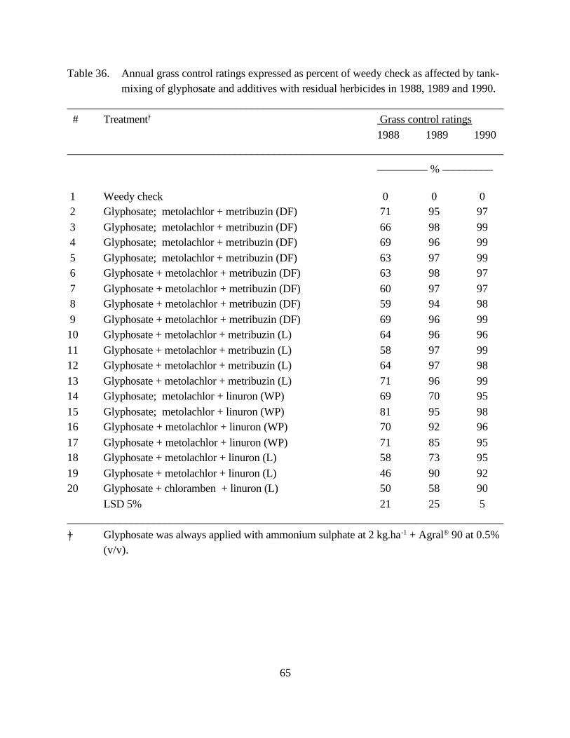
65
Table 36. Annual grass control ratings expressed as percent of weedy check as affected by tank-mixing of glyphosate and additives with residual herbicides in 1988, 1989 and 1990.
______________________________________________________________________________ # Treatment|+ Grass control ratings
1988 1989 1990______________________________________________________________________________
_________ % _________
1 Weedy check 0 0 0 2 Glyphosate; metolachlor + metribuzin (DF) 71 95 97
3 Glyphosate; metolachlor + metribuzin (DF) 66 98 99 4 Glyphosate; metolachlor + metribuzin (DF) 69 96 99
5 Glyphosate; metolachlor + metribuzin (DF) 63 97 99 6 Glyphosate + metolachlor + metribuzin (DF) 63 98 97
7 Glyphosate + metolachlor + metribuzin (DF) 60 97 97 8 Glyphosate + metolachlor + metribuzin (DF) 59 94 98
9 Glyphosate + metolachlor + metribuzin (DF) 69 96 9910 Glyphosate + metolachlor + metribuzin (L) 64 96 96
11 Glyphosate + metolachlor + metribuzin (L) 58 97 9912 Glyphosate + metolachlor + metribuzin (L) 64 97 98
13 Glyphosate + metolachlor + metribuzin (L) 71 96 9914 Glyphosate; metolachlor + linuron (WP) 69 70 95
15 Glyphosate; metolachlor + linuron (WP) 81 95 9816 Glyphosate + metolachlor + linuron (WP) 70 92 96
17 Glyphosate + metolachlor + linuron (WP) 71 85 9518 Glyphosate + metolachlor + linuron (L) 58 73 95
19 Glyphosate + metolachlor + linuron (L) 46 90 9220 Glyphosate + chloramben + linuron (L) 50 58 90
LSD 5% 21 25 5______________________________________________________________________________
|+ Glyphosate was always applied with ammonium sulphate at 2 kg.ha-1 + Agral® 90 at 0.5%(v/v).

66
4.6 COMPATIBILITY OF BURNDOWN AND RESIDUAL HERBICIDES FORQUACKGRASS CONTROL
RESEARCH SUMMARY:
OBJECTIVE : To determine the compatibility of various burn-down and residual herbicide
combinations on quackgrass.
RESULTS :
1) Quackgrass shoot control (as a % of the untreated shoot dry weight) for two doses of
glyphosate, paraquat or glufosinate averaged over three years).
2) Comparisons of split vs. tank-mixed combinations.
Note: -ve sign in tables indicates loss of control when tank-mixed, +ve sign indicates
increase in control when tank-mixed.

67
Table 37. Impact of tank-mixing burndown and residual herbicides on quackgrass control ratingsin 1987, 1988 and 1989.
GLYPHOSATE______________________________________________________________________________
Residual herbicide Glyphosate dose (kg/ha) AverageHerbicide Dose 0.45 0.90 response
of doses______________________________________________________________________________
___________________ % ____________________Linuron (L) 2.25 kg/ha - 5.6 - 27.6 - 16.6
Atrazine (DF) 1.50 kg/ha - 0.8 - 10.2 - 5.5Metribuzin (DF) 0.60 kg/ha - 5.4 - 41.7 - 23.5
Metolachlor 2.64 kg/ha + 13.9 + 10.2 + 12.1______________________________________________________________________________
Table 37 continued ......
PARAQUAT
______________________________________________________________________________ Residual herbicide Paraquat dose (kg/ha) Average
Herbicide Dose 0.50 1.00 response of doses
___________________ % ____________________Linuron (L) 2.25 kg/ha - 14.8 + 6.4 - 4.2
Atrazine (DF) 1.50 kg/ha + 4.5 + 7.7 + 6.1Metribuzin (DF) 0.60 kg/ha + 6.4 + 10.1 + 8.3
Metolachlor 2.64 kg/ha + 8.8 + 5.6 + 7.2______________________________________________________________________________

68
GLUFOSINATE______________________________________________________________________________
Residual herbicide Glufosinate dose (kg/ha) AverageHerbicide Dose 0.50 1.00 response
of doses ___________________ % ____________________
Linuron (L) 2.25 kg/ha + 2.4 - 8.3 - 2.9Atrazine (DF) 1.50 kg/ha + 15.7 + 17.4 + 16.5
Metribuzin (DF) 0.60 kg/ha - 4.4 + 17.7 + 6.7Metolachlor 2.64 kg/ha + 13.1 - 5.4 + 3.9
______________________________________________________________________________
OTHER RESIDUAL HERBICIDES______________________________________________________________________________ Residual herbicide Burndown herbicide
Herbicide Dose Glyphosate Paraquat Glufosinate(0.90 kg/ha) (0.50 kg/ha) (1.0 kg/ha)
_________________________________________________________________________________________________ % ____________________
2,4-D amine 0.50 kg/ha† - 14.6 - 13.9 - 8.02,4-D ester 0.50 kg/ha - 2.4 - 0.6 + 2.6
Dicamba 0.60 kg/ha + 0.5 + 0.5 - 1.6______________________________________________________________________________
2,4-D was applied at 1.50 kg/ha in 1989

69
4.7 RECOMMENDATIONS
On the basis of field experiments conducted at different sites from 1987 to 1990 the
following recommendations are suggested for tank-mixing of various burndown and residual
herbicides in no-till crop production systems:
4.7.1 Paraquat and Glufosinate Antagonism with Residual Herbicides in Corn.
! Paraquat at 0.5 kg.ha-1 can be tank-mixed with recommended label rates of metolachlor +
atrazine (WP or liquid) or cyanazine (WP or liquid) for annual weed control in corn.
! Glufosinate (0.5 to 0.75 kg.ha-1) can be tank-mixed with recommended label rates of
metolachlor + atrazine WG for annual weed control in corn.
4.7.2 Glyphosate Antagonism with Residual Herbicides in the Presence of Additives in No-till Corn.
! Glyphosate from 0.30 to 0.90 kg.ha-1 + ammonium sulphate at 0.2% (v/v) + Agral® 90 at
0.5% (v/v) may be tank-mixed with metolachlor + atrazine, cyanazine, or dicamba at
labelled rates for weed burndown and residual control of annual weeds in corn.
4.7.3 Paraquat and Glufosinate Antagonism with Residual Herbicides in Soybeans.
! Paraquat at 0.5 kg.ha-1 can be tank-mixed with recommended label rates of metolachlor +
metribuzin or linuron for annual weed burndown and subsequent residual weed control.

70
! Glufosinate at 0.50 to 0.75 kg.ha-1 can be tank-mixed with recommended labelled rates of
metolachlor + metribuzin or linuron for annual weed burndown and subsequent residual
weed control.
4.7.4 Glyphosate Antagonism with Residual Herbicides in the Presence of Additives in No-till Soybeans.
! Glyphosate from 0.45 to 0.90 kg.ha-1 + ammonium sulphate at 2 l.ha-1 + Agral® 90 at 0.1%
(v/v) may be tank-mixed with residual herbicides metolachlor + metribuzin or linuron at
labelled rates for burndown and residual control of annual weeds in soybeans.
4.7.5 Antagonism of Paraquat, Glyphosate and Glufosinate with Various Residual
Herbicides for Quackgrass Control! The herbicidal activity of glyphosate was antagonised with tank-mixtures of linuron (L),
atrazine (DF), metribuzin (DF), dicamba or 2,4-D in amine or ester salts at recommended
labelled rates.
! The herbicidal activity of glyphosate was synergised when tank-mixed with metolachlor at
recommended labelled rates.
! The herbicidal activity of paraquat was antagonised with tank-mixtures of linuron (L) or
2,4-D in amine or ester salts at recommended labelled rates.
! The dose of paraquat can be reduced to 0.50 kg.ha-1 from 1.0 kg.ha-1 if tank-mixed with
atrazine, metolachlor or metribuzin at currently recommended rates.
! The herbicidal activity of glufosinate was antagonised with tank-mixtures of linuron (L),
dicamba or amine salt of 2,4-D at recommended labelled rates.
! The herbicidal activity of glufosinate was synergised when tank-mixed with atrazine (DF),
metribuzin (DF), metolachlor or ester salt of 2,4-D at recommended labelled rates.

71
OBJECTIVE # 3
5.0 IMPACT OF TANK-MIXES OF BURNDOWN AND RESIDUAL HERBICIDESWITH ADDITIVES ON WEED CONTROL IN CONSERVATION TILLAGE
SYSTEMS.
Herbicides are marketed in various formulations to improve herbicidal efficacy, shelf-life
and to facilitate their mixing in water. Herbicide formulations usually contain the parent herbicide
molecule and various additives and fillers. However, some of these additives and fillers are
unstable and may react among themselves. Therefore, materials which may not be included in the
manufacturer's formulation may be added to the spray solution just before its actual use. Some of
these additives may be beneficial in terms of improving herbicide efficacy, its spectrum and
economics. It is well documented that various additives may be tank-mixed with herbicides at the
time of spray to increase herbicidal activity or to widen the herbicidal spectrum (O'Sullivan et al.
1983, Turner 1984, Harrison et al. 1986). The use of additives led to an improvement in
herbicidal activity due to enhanced in uptake and translocation of herbicides (Nalewaja and
Skrzyczak 1986, Chandrasena and Sagar 1986). However, some of the additives may also
decrease the biological activity of herbicides on weeds (Harrison et al. 1986, Hallgren and
Nilsson 1986) or reduce crop yields (Witt et al. 1984, Harrison et al. 1986).
This knowledge opened a new horizon of using herbicides with various additives to
improve the weed control in no-till cropping systems. Weed management under a no-till crop
management system is more complex and weed control may be highly variable (Weber and
Lowder, 1985). It was hypothesized that the use of additives in combination with various
burndown and residual herbicides would improve weed management in no-till corn and soybeans

72
in Ontario. Therefore, a series of field experiments were initiated to study the effect of tank-
mixing various herbicides with additives for the control of weeds
in conservation tillage.
5.1 METHODS AND MATERIALS
Field experiments were conducted to evaluate the effect of various herbicides with
additives on the weed burndown effects in no-till systems. The details of experimental procedures
followed and material used are described briefly.
5.1.1. Experimental Locations
Details of experimental locations and soil types of various trials are presented in Table 38.

73
Table 38. Details of experimental locations and soil types for experiments conducted from1987 to 1990.
______________________________________________________________________________Crop Experiment Soil # Site Location Type
Sand Silt Clay O.M. pH______________________________________________________________________________
________ % ________Corn 5.2 Dealtown 42E 15'N Fox Gravelly 59 31 10 2.8 6.1
82E 5' W LoamCorn 5.3 |+ Dealtown 42E 15'N Fox Gravelly 59 31 10 2.8 6.1
82E 5' W LoamCorn 5.4 Clinton 43E 5' N Burford loam 67 23 10 3.9 6.4
(1988) 81E 5' WWoodstock 43E 8' N Sandy loam 53 34 13 3.3 6.8
(1989) 80E 45'WSoybeans 5.5 Dealtown 42E 15'N Fox Gravelly 59 31 10 2.8 6.1
82E 5' W LoamSoybeans 5.6 Clinton 43E 5' N Burford loam 67 23 10 3.9 6.4
(1988) 81E 5' WWoodstock 43E 8'N Sandy loam 53 34 13 3.3 6.8
(1989) 80E 45'WFallow/ 5.7 Elora 42E 27'N Guelph loam 29 53 18 4.3 7.4
Quackgrass 81E 53'W______________________________________________________________________________
|+ Experiment was conducted at Mr. Art Wardle's farm, Ridgetown on Brookston clay loamsoil in 1987.
5.1.2. Agronomy
Experiments were conducted using standard agronomic practices (OMAF publication 296,
Field Crop Recommendations) in no-till plots. Soil samples were taken from each field at the
beginning of the crop season and were analyzed for available nutrient status. Fertilization was

74
done according to soil tests and requirements of individual crops. Fertilizers, if required were
placed at the time of sowing of the crop with minimum soil surface disturbances.
Corn cv. Renk® R148, Dekalb® 524, Renk® R138, Pioneer® 3790, were planted at their
recommended seeding densities in 75 cm rows in 1987, 1988, 1989 and 1990, respectively at
Dealtown or Ridgetown sites. The corn cultivars Pioneer® 3790 and Pioneer® 3925 were planted
at their recommended seeding rates in 76 cm rows at Clinton and Woodstock sites, respectively.
The individual plot size at Dealtown and Ridgetown sites were 6 x 1.5 m and at Clinton and
Woodstock sites 6 x 3 m.
Soybeans cv. Elgin, KG 60 and Pioneer® 0877 were planted in 40 cm rows at a seeding rate
of 70 to 100 kg.ha-1 at Dealtown, Clinton and Woodstock sites, respectively. The individual
soybeans plot sizes were 6 x 1.5 m at Dealtown and at Clinton and Woodstock sites 6 x 3 m.
The quackgrass experiment was established using the quackgrass biotype found at Elora
Research Station, Elora, Ontario. The individual size of quackgrass plots was 6 x 2 m.
Corn and soybeans were harvested from the centre of plots leaving side border rows at
Clinton, Elora and Woodstock sites and from whole plot at Dealtown site. Final yield was later
converted and expressed at 14% and 15.5% moisture content for soybeans and corn, respectively.
Planting, spraying and crop harvesting dates are presented in Table 39.

75
Table 39. Planting, spraying and crop harvesting dates for experiments conducted in 1987,1988, 1989 and 1990.
______________________________________________________________________________Crop Expt. Year Date(s)
# Planting Spraying Harvesting______________________________________________________________________________
Corn 5.2 1988 May 12 May 17 -1989 May 10 May 15 Nov. 9
1990 June 5 May 9 -Corn 5.3 1987 May 13 May 18 -
1988 May 12 May 17 -1989 May 10 May 17 Nov. 9
1990 June 5 May 9 -Corn 5.4 1988 May 6 May 6 Oct. 20
1989 May 17 May 17 Oct. 27Soybeans 5.5 1988 May 19 May 20 -
1989 May 15 May 17 Oct. 271990 May 15 May 14 -
Soybeans 5.6 1988 May 22 May 25 Oct. 31989 May 29 May 25 Oct. 12
Fallow/ 5.7 1986 - Nov. 11 & 17 -Quackgrass† 1987 - Nov. 10 -
______________________________________________________________________________|+ Spring applied herbicides were sprayed on May 5, 1987 and May 17, 1988.
5.1.3 Spraying Equipment and Procedures
Individual plots were sprayed using a 'bicycle sprayer' at Elora, Clinton and Woodstock site
and by an 'Oxford Precision Sprayer' at Dealtown site. The quantity of spray solution used for the
bicycle sprayer was 225 l.ha-1 at 180 kPa. The 'Oxford Precision Sprayer' used 200 l.ha-1 of spray
solution at 240 kPa.

76
5.1.4 Experiment Design and Analysis
All experiments were conducted in randomized complete block design (RCBD) with 4
replications. Results were analyzed using analysis of variance (ANOVA) procedures and means
were then separated using least significant difference (LSD) at 5% level of significance.
5.2 The Role of Additive with Residual Herbicides in Corn
RESEARCH SUMMARY:
Additives Agral® 90, Kornoil concentrate® and Kornoil® when used with different
herbicides provided excellent initial weed burndown and excellent seasonal control of grassy and
broadleaf weeds. Residual herbicides when applied with fertilizer 10-34-0 at higher application
rate (110 L.ha-1) provided average burndown in 1988 and thus this additive was deleted from
treatments in subsequent years. Fertilizer based additives such as 28% N, 10-34-0, Aqua 21% N,
Liquid cyanamid® when applied with residual herbicides also facilitated excellent initial
burndown and subsequent weed control. However, there were some weed escapes.
Overall, the addition of dicamba with metolachlor + atrazine had no additional impact on
the weed control. Dicamba with additives Aqua 21% N or Kornoil concentrate® (COC)
significantly reduced corn yield in 1989.

77
Table 40. Corn yield as affected by various treatments in 1989.
______________________________________________________________________________
# Treatment Dose Yield kg a.i./ha 1989
______________________________________________________________________________ _ kg.ha-1 _
1 check 1720
2 Metol. |++ atra. |=+ Agral 90 2.4 + 1.5 + .1% 6780 3 Metol. + atra. + COC 2.4 + 1.5 + 1% 6700
4 Metol. + atra. + oil 2.4 + 1.5 + 10 L 5970 5 Metol. + atra. + 28% N 2.4 + 1.5 + 10 L 5280
6 Metol. + atra. + 28% N 2.4 + 1.5 + 500 L 7810 7 Metol. + atra. + 10-34-0 2.4 + 1.5 + 10 L 6920
8 Metol. + atra. 2.4 + 1.5 7450 9 Metol. + atra. + aqua 21% N 2.4 + 1.5 + 10 L 6870
10 Metol. + atra. + L.C.§ 2.4 + 1.5 + 10 L 565011 Metol. + atra. + dicamba + Agral 90 2.4 + 1 + .6 + .1% 6220
12 Metol. + atra. + dicamba + COC 2.4 + 1 + .6 + 1 % 473013 Metol. + atra. + dicamba + oil 2.4 + 1 + .6 + 10 L 5290
14 Metol. + atra. + dicamba + 28% N 2.4 + 1 + .6 + 10 L 578015 Metol. + atra. + dicamba + 28% N 2.4 + 1 + .6 + 500 L 6300
16 Metol. + atra. + dicamba + 10-34-0 2.4 + 1 + .6 + 10 L 592017 Metol. + atra. + dicamba 2.4 + 1 + .6 6240
18 Metol. + atra. + dicamba + aqua 21% N 2.4 + 1 + .6 + 10 L 495019 Metol. + atra. + dicamba + L.C. 2.4 + 1 + .6 + 10 L 6300
20 Metol. + atra. + dicamba + 28% N + COC 2.4 + 1 + .6 + 10 L+1% 6280LSD 5% 1530
______________________________________________________________________________|+ metolachlor
|= atrazine§ Liquid cyanamid®

78
Table 41. Initial annual weed burndown ratings expressed as percent of weedy check as affectedby residual herbicides with additives in 1988, 1989 and 1990.
______________________________________________________________________________ # Treatment Weed burndown ratings
1988 1989 1990______________________________________________________________________________
____________ % ___________
1 Weedy check 0 0 0 2 Metol. |++ atrazine + Agral 90 97 98 98
3 Metol. + atrazine + COC 96 93 91 4 Metol. + atrazine + oil 98 86 89
5 Metol. + atrazine + 28% N 97 65 86 6 Metol. + atrazine + 28% N 91 99 91
7 Metol. + atrazine + 10-34-0 99 90 86 8 Metol. + atrazine 75 90 88
9 Metol. + atrazine + aqua 21% N 93 99 7810 Metol. + atrazine + L.C. |= 84 95 91
11 Metol. + atrazine + dicamba + Agral 90 99 96 9712 Metol. + atrazine + dicamba + COC 99 95 98
13 Metol. + atrazine + dicamba + oil 87 99 9314 Metol. + atrazine + dicamba + 28% N 96 99 88
15 Metol. + atrazine + dicamba + 28% N 93 97 8716 Metol. + atrazine + dicamba + 10-34-0 79 96 76
17 Metol. + atrazine + dicamba 74 99 7918 Metol. + atrazine + dicamba + aqua 21% N 88 88 83
19 Metol. + atrazine + dicamba + L.C. 76 97 9120 Metol. + atrazine + dicamba + 28% N + COC 91 97 95
LSD 5% 20 21 16______________________________________________________________________________
|+ metolachlor|= Liquid cyanamid®

79
Table 42. Broadleaf weed control ratings expressed as percent of weedy check as affected byresidual herbicides with additives in 1988, 1989 and 1990.
______________________________________________________________________________ # Treatment Broadleaf control ratings
1988 1989 1990______________________________________________________________________________
___________ % ___________
1 Weedy check 0 0 0 2 Metol. |++ atrazine + Agral 90 82 98 99
3 Metol. + atrazine + COC 80 98 95 4 Metol. + atrazine + oil 78 98 97
5 Metol. + atrazine + 28% N 77 65 96 6 Metol. + atrazine + 28% N 75 99 96
7 Metol. + atrazine + 10-34-0 80 93 96 8 Metol. + atrazine 78 98 96
9 Metol. + atrazine + aqua 21% N 93 100 9310 Metol. + atrazine + L.C. |= 80 99 98
11 Metol. + atrazine + dicamba + Agral 90 82 99 9812 Metol. + atrazine + dicamba + COC 83 96 90
13 Metol. + atrazine + dicamba + oil 83 99 9214 Metol. + atrazine + dicamba + 28% N 80 99 95
15 Metol. + atrazine + dicamba + 28% N 80 99 9616 Metol. + atrazine + dicamba + 10-34-0 80 96 91
17 Metol. + atrazine + dicamba 80 100 9318 Metol. + atrazine + dicamba + aqua 21% N 77 99 93
19 Metol. + atrazine + dicamba + L.C. 68 98 9620 Metol. + atrazine + dicamba + 28% N + COC 67 98 97
LSD 5% 17 15 7______________________________________________________________________________
|+ metolachlor|= Liquid cyanamid®
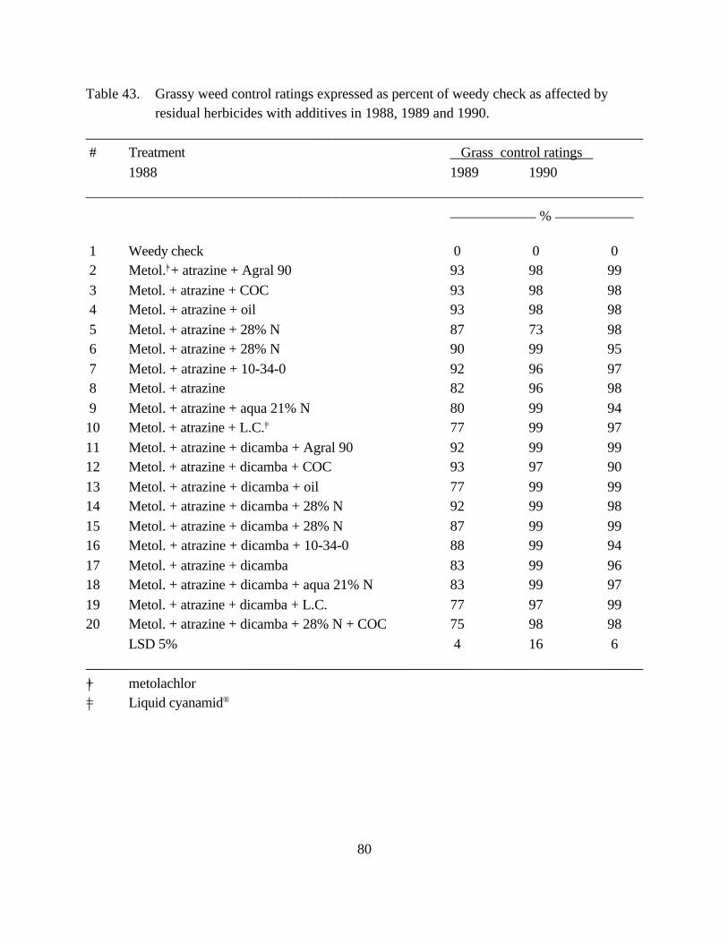
80
Table 43. Grassy weed control ratings expressed as percent of weedy check as affected byresidual herbicides with additives in 1988, 1989 and 1990.
______________________________________________________________________________ # Treatment Grass control ratings
1988 1989 1990______________________________________________________________________________
____________ % ___________
1 Weedy check 0 0 0 2 Metol. |++ atrazine + Agral 90 93 98 99
3 Metol. + atrazine + COC 93 98 98 4 Metol. + atrazine + oil 93 98 98
5 Metol. + atrazine + 28% N 87 73 98 6 Metol. + atrazine + 28% N 90 99 95
7 Metol. + atrazine + 10-34-0 92 96 97 8 Metol. + atrazine 82 96 98
9 Metol. + atrazine + aqua 21% N 80 99 9410 Metol. + atrazine + L.C. |= 77 99 97
11 Metol. + atrazine + dicamba + Agral 90 92 99 9912 Metol. + atrazine + dicamba + COC 93 97 90
13 Metol. + atrazine + dicamba + oil 77 99 9914 Metol. + atrazine + dicamba + 28% N 92 99 98
15 Metol. + atrazine + dicamba + 28% N 87 99 9916 Metol. + atrazine + dicamba + 10-34-0 88 99 94
17 Metol. + atrazine + dicamba 83 99 9618 Metol. + atrazine + dicamba + aqua 21% N 83 99 97
19 Metol. + atrazine + dicamba + L.C. 77 97 9920 Metol. + atrazine + dicamba + 28% N + COC 75 98 98
LSD 5% 4 16 6______________________________________________________________________________
|+ metolachlor|= Liquid cyanamid®

81
Table 44. Total weed biomass accumulation as affected by various treatments in 1989 and 1990.______________________________________________________________________________
# Treatment Total weed biomass Broadleaf Grasses
1989 1990 1989 1990______________________________________________________________________________
g.m-1
1 check 1442 1363 658 6 2 Metol. |++ atra. |=+ Agral 90 128 279 100 66
3 Metol. + atra. + COC 174 383 200 129 4 Metol. + atra. + oil 76 539 78 0
5 Metol. + atra. + 28% N 496 405 86 2 6 Metol. + atra. + 28% N 186 270 134 49
7 Metol. + atra. + 10-34-0 276 762 172 0 8 Metol. + atra. 126 187 194 63
9 Metol. + atra. + aqua 21% N 34 623 110 810 Metol. + atra. + L.C.§ 96 12 110 392
11 Metol. + atra. + dicamba+ Agral 90 110 202 236 412 Metol. + atra. + dicamba + COC 102 494 286 12
13 Metol. + atra. + dicamba + oil 152 166 168 3314 Metol. + atra. + dicamba + 28% N 386 79 98 142
15 Metol. + atra. + dicamba + 28% N 214 542 30 5216 Metol. + atra. + dicamba + 10-34-0 108 548 84 111
17 Metol. + atra. + dicamba 134 272 176 418 Metol. + atra. + dicamba + aqua 21% N 206 260 104 48
19 Metol. + atra. + dicamba + L.C. 282 341 656 620 Metol. + atra. + dicamba + 28% N + COC 114 154 82 119
LSD 5% 436 593 364 213______________________________________________________________________________
|+ metolachlor|= atrazine
§ Liquid cyanamid®
82
5.3 Herbicides for Burndown and Residual Control of Annual Weeds in No-till Corn
RESEARCH SUMMARY:
Residual herbicides provided satisfactory to excellent burndown of annual and perennial
weed species. Cyanazine with atrazine or glufosinate provided excellent early-season weed
burndown. Burndown herbicides glufosinate and paraquat in combination with residual herbicides
metolachlor, dicamba, metribuzin, cyanazine, atrazine or SAN S82 were also excellent treatments
for broad spectrum burndown activity.
Late emerging broad-leaved weed control by various residual herbicides was also
satisfactory to excellent. Atrazine + linuron or metribuzin with burndown herbicides were very
effective in controlling late-emerging broadleaf weeds in 1988, 1989 and 1990. However, in
1987 scentless chamomile escaped these herbicides resulting in overall poor broadleaf weed
control. Similarly, redroot pigweed escaped glufosinate + cyanazine in 1988. Linuron alone or in
combination with metolachlor or glufosinate failed to control pineapple weed in 1989.
Residual herbicides provided excellent control of late emerging grasses. However, there
were a few exceptions. Atrazine + DPX 6316 failed to control barnyardgrass in 1988 and green
foxtail in 1989. Similarly, barnyard grass, green foxtail and downeybrome escaped linuron or
metribuzin treated plots in 1989.
Corn yields were significantly reduced in treatments receiving linuron or atrazine/dicamba
in 1989. This may be due to a poor weed control provided by these herbicides. Metribuzin
treated plots also had poor corn yields as this herbicide caused significant crop injury at the
beginning of the growing season.

83
Table 45. Corn yield as affected by various treatments in 1989.
_____________________________________________________________________________
# Treatment|+ Dose Yield kg a.i./ha 1989
______________________________________________________________________________ _ kg/ha _
1 Weedy check 1880
2 Atrazine 1.5 5110 3 Cyanazine 2.5 5020
4 Cyanazine + atrazine 2.5 + 1.5 7100 5 Linuron 2.0 2450
6 Metribuzin 0.75 3930 7 Linuron + metribuzin 1 + 0.5 4620
8 Metolachlor + linuron 2.4 + 1.0 3660 9 Metolachlor + metribuzin 2.4 + 0.5 4900
10 Metolachlor + atrazine + linuron 2.4 + 1 + 1 685011 CGA 180937 + atrazine + linuron 2.3 + 1 + 1 5670
12 CGA 180937 + metribuzin 2.3 + 0.5 461013 Dicamba/atrazine 1.75 3810
14 Dicamba/atrazine 1.75 3720 15 Glufosinate + linuron 0.75 + 2 2990
16 Glufosinate + metolachlor + dicamba 0.75 + 2.4 + .6 514017 Glufosinate + metribuzin 0.75 + 0.75 3970
18 Glufosinate + cyanazine 0.75 + 2.25 7060 19 DPX M6316 + atrazine 0.012 + 1.5 5820
20 Paraquat + SAN 582 + atrazine 0.5 + 1.25 + 1 5750
LSD 5% 1850 ___________________________________________________________________________
|+ treatments except 12 were applied with Kornoil concentrate® at 1% (v/v).

84
Table 46. Initial weed burndown ratings expressed as percent of weedy check as affected byvarious treatments in 1988,1989 and 1990.
______________________________________________________________________________ # Treatment Weed burndown ratings
1988 1989 1990______________________________________________________________________________
___________ % __________
1 Weedy check 0 0 0 2 Atrazine + COC† 100 94 69
3 Cyanazine + COC 83 94 81 4 Cyanazine + atrazine + COC 96 100 99
5 Linuron + COC 99 63 88 6 Metribuzin + COC 91 88 69
7 Linuron + metribuzin + COC 98 97 89 8 Metolachlor + linuron + COC 99 60 55
9 Metolachlor + metribuzin + COC 96 91 7810 Metolachlor + atrazine + linuron + COC 84 93 83
11 CGA 180937 + atrazine + linuron + COC 98 92 6712 CGA 180937 + metribuzin + COC 99 97 56
13 Dicamba/atrazine 87 79 9314 Dicamba/atrazine + COC 99 75 95
15 Glufosinate + linuron + COC 91 46 9416 Glufosinate + metolachlor + dicamba + COC 99 71 92
17 Glufosinate + metribuzin + COC 97 96 9918 Glufosinate + cyanazine + COC 92 99 100
19 DPX M6316 + atrazine + COC 86 98 9620 Paraquat + SAN 582 + atrazine + COC 92 99 97
LSD 5% 12 19 24______________________________________________________________________________
† Kornoil concentrate®

85
Table 47. Broadleaf weed control ratings expressed as percent of weedy check as affected bypreemergence herbicides with additives in 1987, 1988, 1989 and 1990.
______________________________________________________________________________ # Treatment Broadleaf weed control
1987 1988 1989 1990______________________________________________________________________________
_____________ % ____________
1 Weedy check 0 0 0 0 2 Atrazine + COC† 85 70 85 80
3 Cyanazine + COC 85 66 85 82 4 Cyanazine + atrazine + COC 80 78 97 98
5 Linuron + COC 81 66 83 85 6 Metribuzin + COC 80 74 97 95
7 Linuron + metribuzin + COC 81 78 98 96 8 Metolachlor + linuron + COC 81 76 68 95
9 Metolachlor + metribuzin + COC 83 80 90 9810 Metolachlor + atrazine + linuron + COC 81 79 89 98
11 CGA 180937 + atrazine + linuron + COC 60 73 98 9712 CGA 180937 + metribuzin + COC 74 71 98 97
13 Dicamba/atrazine 80 80 83 9714 Dicamba/atrazine + COC 81 82 81 98
15 Glufosinate + linuron + COC 83 78 53 9516 Glufosinate + metolachlor + dicamba + COC 81 84 71 91
17 Glufosinate + metribuzin + COC 83 75 95 9818 Glufosinate + cyanazine + COC 83 60 85 92
19 DPX M6316 + atrazine + COC 81 56 90 9820 Paraquat + SAN 582 + atrazine + COC 83 76 97 84
LSD 5% 14 20 2416
______________________________________________________________________________† Kornoil concentrate®

86
Table 48. Annual grass control ratings expressed as percent of weedy check as affected bypreemergence herbicides with additives in 1987, 1988, 1989 and 1990.
______________________________________________________________________________ # Treatment Grass weed control
1987 1988 1989 1990______________________________________________________________________________
_____________ % ____________
1 Weedy check 0 0 0 0 2 Atrazine + COC† 13 85 75 79
3 Cyanazine + COC 0 79 78 87 4 Cyanazine + atrazine + COC 0 84 90 98
5 Linuron + COC 0 81 50 82 6 Metribuzin + COC 0 89 61 94
7 Linuron + metribuzin + COC 0 89 90 98 8 Metolachlor + linuron + COC 0 89 91 98
9 Metolachlor + metribuzin + COC 0 89 95 9910 Metolachlor + atrazine + linuron + COC 13 84 94 99
11 CGA 180937 + atrazine + linuron + COC 25 85 94 9912 CGA 180937 + metribuzin + COC 0 89 93 98
13 Dicamba/atrazine 19 74 66 9514 Dicamba/atrazine + COC 0 90 70 87
15 Glufosinate + linuron + COC 6 86 74 9916 Glufosinate + metolachlor + dicamba + COC 0 88 90 98
17 Glufosinate + metribuzin + COC 20 79 95 9118 Glufosinate + cyanazine + COC 0 75 91 98
19 DPX M6316 + atrazine + COC 0 63 73 9220 Paraquat + SAN 582 + atrazine + COC 13 78 95 95
LSD 5% NS 12 19 17______________________________________________________________________________
† Kornoil concentrate®

87
5.4 Annual Weed Control in No-till Corn by Residual Herbicides Applied With Additives
RESEARCH SUMMARY:
Experiments were conducted at Clinton in 1988 and at the Woodstock Research Station in
1989. Common ragweed (Ambrosia artemisiifolia L.) was the pre-dominant weed species at
Clinton and lamb's-quarters (Chenopodium album L.) at Woodstock, redroot pigweed (Amaranthus
retroflexus L.) and common ragweed.
All residual herbicides provided excellent annual weed control in 1988. However, in 1989,
atrazine resistant redroot pigweed and lamb's-quarters biotypes escaped all atrazine treatments.
Linuron and dicamba provided excellent lamb's-quarters control but dicamba failed to control
redroot pigweed which continued to emerge later in the season. Linuron failed to provide control
of Canada fleabane.
Corn yields were not affected by the presence of weeds in 1988. However, in 1989, crop
injury resulting from dicamba + metolachlor significantly reduced corn yield.
The addition of 28% N and Kornoil concentrate® had no impact on weed control in both
years. However, in contrast additives increased corn injury by dicamba + metolachlor, which
resulted in further corn yield losses.

88
Table 49. Corn yield as affected by various treatments in 1988 and 1989.
______________________________________________________________________________ # Treatment Dose Corn yield
kg a.i./ha 1988 1989______________________________________________________________________________
___ kg.ha-1 ___
1 Weedy 6150 3880 2 Paraquat 1.0 6720 7190
3 Paraquat + atrazine + metol. |+ 1.0 + 2.0 + 2.64 5660 8500 4 Atrazine 1.5 6000 9090
5 Atrazine + metol. 1.5 + 1.92 6530 7140 6 Cyanazine + metol. 2.0 + 1.92 6670 8170
7 Linuron + metol. 1.1 + 1.92 5680 7490 8 Dicamba + metol. 0.6 + 1.92 6510 6650
9 Atrazine + 28% N 1.5 + 5% 5790 764010 Atrazine + metol. + 28% N 1.5 + 1.92 + 5% 7000 8180
11 Cyanazine + metol. + 28% N 2.0 + 1.92 + 5% 6780 905012 Linuron + metol. + 28% N 1.1 + 1.92 + 5% 6080 7870
13 Dicamba + metol. + 28% N 0.6 + 1.92 + 5% 5920 640014 Atrazine + COC |= 1.5 + 1% 7340 8360
15 Atrazine + metol. + COC 1.5 + 1.92 + 1% 7040 827016 Cyanazine + metol. + COC 2.0 + 1.92 + 1% 7170 9280
17 Linuron + metol. + COC 1.1 + 1.92 + 1% 5810 812018 Dicamba + metol. + COC 0.6 + 1.92 + 1% 6000 6160
LSD 5% NS 1520______________________________________________________________________________
|+ metolachlor|= Kornoil concentrate®

89
Table 50. Annual weed control ratings expressed as percent of weedy check as affected bypreemergence herbicides with additive in 1988 and 1989.
______________________________________________________________________________ # Treatment Weed control ratings
Ragweed Pigweed LQ |+ Fleabane1988 1989 1989 1989 1989
_________________________________________________________________________________________________ % _________________
1 Weedy check 0 0 0 0 0
2 Paraquat 65 98 5 60 53 3 Paraquat + atrazine + metol. |= 99 100 55 45 100
4 Atrazine 95 98 43 43 100 5 Atrazine + metol. 98 100 78 8 100
6 Cyanazine + metol. 95 100 38 38 100 7 Linuron + metol. 93 100 70 98 0
8 Dicamba + metol. 96 88 23 88 100 9 Atrazine + 28% N 93 100 75 38 100
10 Atrazine + metol. + 28% N 99 100 58 30 10011 Cyanazine + metol. + 28% N 98 100 35 28 100
12 Linuron + metol. + 28% N 89 100 85 93 013 Dicamba + metol. + 28% N 100 93 45 95 100
14 Atrazine + COC§ 100 100 18 23 10015 Atrazine + metol. + COC 100 100 68 33 100
16 Cyanazine + metol. + COC 95 100 20 50 10017 Linuron + metol. + COC 94 88 63 88 20
18 Dicamba + metol. + COC 98 100 33 80 100LSD 5% 14 11 33 33 13
______________________________________________________________________________|+ lamb's-quarters
|= metolachlor§ Kornoil concentrate®

90
5.5 Burndown and Residual Weed Control in Soybeans
RESEARCH SUMMARY:
Excellent weed burndown was achieved by various combinations of herbicides and
additives in this experiment. Metribuzin with the additive Agral® 90 gave poor burndown in 1988,
average in 1990 but satisfactory burndown in 1989. The weather in 1989 was favourable for
excellent herbicidal activity, hence additives to improve the performance of residual herbicides as
burndown treatments were not required.
Linuron in combination with selected additives exhibited excellent broadleaf weed control
except when used with COC in 1990. Monolinuron with additive '10-34-0 fertilizer' gave poor
results in all three years.
Linuron also provided excellent grassy weed control with all additive combinations.
However, grassy weed control with metribuzin and Kornoil® was unsatisfactory in all three years.

91
Table 51. Soybeans yield as affected by various preemergence herbicides applied with additivesin 1989.
______________________________________________________________________________
# Treatment Dose Yield
kg a.i./ha 1989
_ kg/ha _
1 Check 1120
2 Metolachlor + metribuzin + Agral 90 2.4 + 0.6 + .1% 3080
3 Metolachlor + metribuzin + COC 2.4 + 0.6 + 1% 2660
4 Metolachlor + metribuzin + oil 2.4 + 0.6 + 10 L 3200
5 Metolachlor + metribuzin + 28% N 2.4 + 0.6 + 10 L 3300
6 Metolachlor + metribuzin + Aqua 21% N+| 2.4 + 0.6 + 10 L 2930
7 Metolachlor + metribuzin + 10-34-0 2.4 + 0.6 + 10 L 2980
8 Metolachlor + metribuzin + Liq. cyanamid® 2.4 + 0.6 + 10 L 2930
9 Metolachlor + linuron + Agral 90 2.4 + 2.0 + 0.1% 3090
10 Metolachlor + linuron + COC 2.4 + 2.0 + 1% 3180
11 Metolachlor + linuron + oil 2.4 + 2.0 + 10 L 2810
12 Metolachlor + linuron + 28% N 2.4 + 2.0 + 10 L 2740
13 Metolachlor + linuron + Aqua 21% N 2.4 + 2.0 + 10 L 3170
14 Metolachlor + linuron + 10-34-0 2.4 + 2.0 + 10 L 2870
15 Metolachlor + linuron + Liq. cyanamid® 2.4 + 2.0 + 10 L 2440
16 Metolachlor + monolinuron + COC 2.4 + 2.0 + 1 % 2970
17 Metolachlor + monolinuron + oil 2.4 + 2.0 + 10 L 3000
18 Metolachlor + monolinuron + 28% N 2.4 + 2.0 + 10 L 2430
19 Metolachlor + monolinuron + 10-34-0 2.4 + 2.0 + 10 L 2520
20 Metolachlor + monolinuron + Liq. cyanamid® 2.4 + 2.0 + 10 L 2520
LSD 5% 800
______________________________________________________________________________
|+ aqua 21% N was tank-mixed in 1988 only.

92
Table 52. Initial weed burndown expressed as percent of weedy check as affected by varioustreatments in 1988, 1989 and 1990.
# Treatment Weed burndown ratings
1988 1989 1990
__________ % __________
1 Weedy check 0 0 0 2 Metolachlor + metribuzin + Agral 90 63 100 71
3 Metolachlor + metribuzin + COC 60 100 72 4 Metolachlor + metribuzin + oil 57 100 72
5 Metolachlor + metribuzin + 28% N 82 99 86 6 Metolachlor + metribuzin + Aqua 21% N |+ 78 100 80
7 Metolachlor + metribuzin + 10-34-0 82 100 97 8 Metolachlor + metribuzin + Liq. cyanamid® 65 100 88
9 Metolachlor + linuron + Agral 90 80 99 9310 Metolachlor + linuron + COC 83 99 73
11 Metolachlor + linuron + oil 82 100 40 12 Metolachlor + linuron + 28% N 85 99 61
13 Metolachlor + linuron + Aqua 21% N 93 98 3814 Metolachlor + linuron + 10-34-0 90 99 94
15 Metolachlor + linuron + Liq. cyanamid® 88 99 88 16 Metolachlor + monolinuron + COC 85 100 84
17 Metolachlor + monolinuron + oil 80 97 8518 Metolachlor + monolinuron + 28% N 90 92 82
19 Metolachlor + monolinuron + 10-34-0 82 89 6820 Metolachlor + monolinuron + Liq. cyanamid® 82 94 80
LSD 5% 19 6 36
|+ aqua 21% N was tank-mixed in 1988 only.

93
Table 53. Annual broadleaf weed control ratings expressed as percent of weedy check asaffected by various treatments in 1988, 1989 and 1990.
# Treatment Broadleaf ratings
1988 1989 1990______________________________________________________________________________
__________ % __________
1 Weedy check 0 0 0 2 Metolachlor + metribuzin + Agral 90 25 88 91
3 Metolachlor + metribuzin + COC 35 88 87 4 Metolachlor + metribuzin + oil 37 88 82
5 Metolachlor + metribuzin + 28% N 35 91 88 6 Metolachlor + metribuzin + Aqua 21% N |+ 40 91 93
7 Metolachlor + metribuzin + 10-34-0 40 92 94 8 Metolachlor + metribuzin + Liq. cyanamid® 18 88 86
9 Metolachlor + linuron + Agral 90 43 96 7210 Metolachlor + linuron + COC 45 97 62
11 Metolachlor + linuron + oil 50 96 8012 Metolachlor + linuron + 28% N 48 97 88
13 Metolachlor + linuron + Aqua 21% N 42 96 8714 Metolachlor + linuron + 10-34-0 50 98 94
15 Metolachlor + linuron + Liq. cyanamid® 52 95 7416 Metolachlor + monolinuron + COC 37 96 84
17 Metolachlor + monolinuron + oil 37 92 8818 Metolachlor + monolinuron + 28% N 35 87 90
19 Metolachlor + monolinuron + 10-34-0 30 85 6420 Metolachlor + monolinuron + Liq. cyanamid® 32 94 59
LSD 5% 20 9 22______________________________________________________________________________
|+ aqua 21% N was tank-mixed in 1988 only.

94
Table 54. Annual grassy weed control ratings expressed as percent of weedy check as affectedby various treatments in 1988, 1989 and 1990.
# Treatment Grass control ratings
1988 1989 1990______________________________________________________________________________
__________ % __________
1 Weedy check 0 0 0 2 Metolachlor + metribuzin + Agral 90 37 96 98
3 Metolachlor + metribuzin + COC 37 90 98 4 Metolachlor + metribuzin + oil 23 82 88
5 Metolachlor + metribuzin + 28% N 40 93 98 6 Metolachlor + metribuzin + Aqua 21% N† 30 96 99
7 Metolachlor + metribuzin + 10-34-0 33 95 99 8 Metolachlor + metribuzin + Liq. cyanamid® 33 97 99
9 Metolachlor + linuron + Agral 90 43 97 9710 Metolachlor + linuron + COC 53 99 99
11 Metolachlor + linuron + oil 53 96 92 12 Metolachlor + linuron + 28% N 50 97 98
13 Metolachlor + linuron + Aqua 21% N 43 97 9914 Metolachlor + linuron + 10-34-0 47 99 99
15 Metolachlor + linuron + Liq. cyanamid® 47 99 9416 Metolachlor + monolinuron + COC 37 97 98
17 Metolachlor + monolinuron + oil 43 94 9818 Metolachlor + monolinuron + 28% N 33 97 99
19 Metolachlor + monolinuron + 10-34-0 40 93 9920 Metolachlor + monolinuron + Liq. cyanamid® 43 96 96
LSD 5% 15 10 8______________________________________________________________________________
|+ aqua 21% N was tank-mixed in 1988 only.

95
5.6 Annual Weed Control in No-till Soybeans by Residual Herbicides Applied WithAdditives
RESEARCH SUMMARY:
Imazethapyr provided excellent control of yellow nut sedge, wild buckwheat; satisfactory
control of common ragweed and lamb's-quarters, but poor control of Canada fleabane. Linuron
was very effective on lamb's-quarters but gave very poor control of yellow nut sedge and Canada
fleabane. Metribuzin failed to control lamb's-quarters and yellow nut sedge. Ragweed was
controlled by various herbicides with the exception of the lower dose of linuron + metribuzin.
Most of the ragweed emerged at the time of herbicide application (prior to crop emergence).
Paraquat provided excellent control of all emerged weed species. Additives did not have a major
impact on weed control.
Soybean yields were not affected by weeds in 1988 as the predominant weed species,
ragweed was present at very low densities (1-2 weeds.m-2). Soybean yields from all herbicide
treatments were not significantly reduced compared to the yields of the weed-free treatments.
Linuron at higher doses or metribuzin applied without additives were not able to control the pre-
dominant weed species of yellow nut sedge and lamb's-quarters, respectively. As a result,
soybeans yields in these treatments were reduced compared to the weed-free soybeans yields.

96
Table 55. Soybeans yield as affected by various treatments in 1988 and 1989.
______________________________________________________________________________
# Treatment Dose Soybeans yieldkg a.i./ha 1988 1989
__________________________________________________________________________________ kg.ha-1 ___
1 Weedy 2860 640
2 Paraquat 1.0 3180 1900 3 Paraquat + linuron + metol. |+ 1.0 + 0.85 + 1.68 3250 2870
4 Imazethapyr 0.15 3150 1610 5 Linuron 2.25 3110 1000
6 Metribuzin 0.60 3000 1300 7 Linuron + metol. 0.85 + 1.68 2970 1440
8 Metribuzin + metol. 0.85 + 1.68 2980 2380 9 Imazethapyr+ COC|= 0.15 + 1% 3230 1610
10 Linuron + COC 2.25 + 1% 2930 107011 Metribuzin + COC 0.60 + 1% 2970 1980
12 Linuron + metol. + COC 0.86 + 1.68 + 1% 2850 230013 Metribuzin + metol. + COC 0.60 + 1.68 + 1% 3220 1970
14 Imazethapyr+ 28% N 0.15 + 5% 3170 146015 Linuron + 28% N 2.25 + 5% 3060 1080
16 Metribuzin + 28% N 0.60 + 5% 3080 161017 Linuron + metol. + 28% N 0.85 + 1.68 + 5% 2950 2050
18 Metribuzin + metol. + 28% N 0.60 + 1.68 + 5% 3260 2040LSD 5% NS 930
______________________________________________________________________________|+ metolachlor
|= Kornoil concentrate®

97
Table 56. Weed control ratings expressed as percent of weedy check as affected by herbicideswith additives in 1988 and 1989.
______________________________________________________________________________ # Treatment Weed control ratings
Ragweed Nutsedge Buckweed Fleabane 1988 1989 1989 1989 1989
________________________________________________________________________________________________ % ___________________
1 Weedy check 0 0 0 0 0
2 Paraquat 81 23 30 90 43 3 Paraquat + linuron+ metol. |+ 84 40 100 95 70
4 Imazethapyr 80 99 100 73 8 5 Linuron 89 13 100 100 0
6 Metribuzin 85 25 100 0 100 7 Linuron + metol. 64 63 100 100 8
8 Metribuzin + metol. 78 38 100 28 95 9 Imazethapyr + COC|= 69 99 100 88 25
10 Linuron + COC 83 23 100 100 011 Metribuzin + COC 88 40 100 38 75
12 Linuron + metol. + COC 60 60 100 100 2513 Metribuzin + metol. + COC 78 35 100 30 73
14 Imazethapyr + 28% N 84 98 100 63 2315 Linuron + 28% N 93 8 100 100 3
16 Metribuzin + 28% N 73 23 100 25 10017 Linuron + metol.+ 28% N 73 88 100 98 25
18 Metribuzin + metol.+ 28% N 84 83 100 35 95LSD 5% 17 36 12 38 36
______________________________________________________________________________|+ metolachlor
|= Kornoil concentrate®

98
5.7 Preemergence and Postemergence Herbicides for Control of Quackgrass
RESEARCH SUMMARY:
Quackgrass control was significantly improved with spring applied glyphosate or
quizalofop as compared to the fall application. Quackgrass control early in the season by spring
applied glyphosate or quizalofop was similar in both years. However, by late August, glyphosate
treated plots had significantly fewer quackgrass plants.m-2 as compared to the quizalofop treated
plots.
Glyphosate or quizalofop when applied in fall as pre-harvest application had better early-
season quackgrass control than their post-harvest application. However, later in the season, there
was no apparent difference in quackgrass control by either pre-harvest or post-harvest herbicide
application.
The additive Frigate® enhanced quackgrass control by glyphosate. A lower dose of
glyphosate (0.9 l.ha-1) with Frigate had statistically similar quackgrass control as compared to a
higher dose of glyphosate (1.8 l.ha-1) without Frigate. Glyphosate at 0.45 kg.ha-1 was also very
effective when applied in the spring.

99
Table 57. Quackgrass shoot control ratings expressed as percent of weedy check as affected by thetime of application of various burndown herbicides in 1987 and 1988.
______________________________________________________________________________# Treatment|+ Dose Applied Quackgrass Control
kg a.i./ha 1987 |= 1988______________________________________________________________________________
_________ % ________
1 Weedy Check 0 0 0 0 2 Quizalofop 0.096 Pre- harvest 68 24 0 15
3 Quizalofop 0.096 Post-harvest 15 3 0 18 4 Quizalofop 0.144 Pre- harvest 73 6 0 8
5 Quizalofop 0.144 Post-harvest 38 3 0 15 6 Quizalofop 0.192 Pre- harvest 76 26 3 19
7 Quizalofop 0.192 Post-harvest 33 13 3 24 8 Glyphosate + Frigate 0.450 + 0.5% Pre- harvest 83 56 15 29
9 Glyphosate + Frigate 0.450 + 0.5% Post-harvest 54 11 0 2810 Glyphosate + Frigate 0.900 + 0.5% Pre- harvest 84 71 18 25
11 Glyphosate + Frigate 0.900 + 0.5% Post-harvest 70 26 3 4012 Glyphosate 1.800 Pre- harvest 85 70 25 43
13 Glyphosate 1.800 Post-harvest 73 40 3 4814 Quizalofop 0.096 Spring - 85 23 94
15 Quizalofop 0.144 Spring - 89 30 9416 Quizalofop 0.192 Spring - 88 46 94
17 Glyphosate + Frigate 0.450 + 0.5% Spring - 94 73 9618 Glyphosate + Frigate 0.900 + 0.5% Spring - 95 80 95
19 Glyphosate 1.800 Spring - 95 81 96LSD 5% 14 11 6 15
_____________________________________________________________________________|+ Quizalofop was applied with Canplus® 411 at 1% (v/v). Treatment 8, 9 and 17were applied
with ammonium sulphate at 3 l.ha-1. |= quackgrass control ratings were recorded on may 5, june 15 and aug 25 in 1987 and on june
27 in 1988.

100
5.8 RECOMMENDATIONS
On the basis of field experiments conducted at various sites from 1987 to 1990 the
following recommendations are suggested for the use of additives with various residual and
burndown herbicides in no-till crop management systems.
5.8.1 The Role of Additives With Residual Herbicides in No-till Corn
! Metolachlor + atrazine or metolachlor + atrazine + dicamba at labelled rates may be
sprayed with additives Agral® 90 at 0.1% (v/v), Kornoil concentrate® at 1% (v/v),
Kornoil® at 10 l.ha-1, 28% N at 500 l.ha-1, 10-34-0 at 10 l.ha-1, Aqua 21% N at 10 l.ha-1 for
burndown and residual annual weed control in corn.
5.8.2 Herbicides for Burndown and Residual Control of Annual Weeds in No-till Corn
! Atrazine at 1.5 kg.ha-1, cyanazine at 2.5 kg.ha-1 or atrazine at 1.5 kg.ha-1 + cyanazine at 2.5
kg.ha-1 with 1% solution (v/v) of Kornoil concentrate®.
! Linuron at 1 kg.ha-1 + metribuzin at 0.5 kg.ha-1 or linuron at 1 kg.ha-1 + atrazine (1 kg. ha-1)
+ metolachlor (2.4 kg.ha-1) with 1% Kornoil concentrate®.
! Glufosinate at 0.75 kg.ha-1 + metribuzin at 0.75 kg.ha-1 with 1% solution (v/v) of Kornoil
concentrate®.

101
5.8.3 Annual Weed Control in No-till Corn by Residual Herbicides AppliedWith Additives
! For control of common ragweed seedlings, atrazine, cyanazine, linuron or dicamba at
labelled rates, applied preemergence to corn.
! Additives such as 28% N at 5% (v/v) or Kornoil concentrate® at 1% (v/v) may be added
with these herbicides.
5.8.4 Burndown and Residual Weed Control in No-till Soybeans
! Metolachlor (2.4 kg.ha-1) + metribuzin (0.6 kg.ha-1) should be applied with additives 28%
N or 10-34-0 at 10 l.ha-1 for effective annual weed control in soybeans.
! Metolachlor at 2.4 kg.ha-1 + linuron at 2 kg.ha-1 should be applied with additives Agral® 90
at 0.1% (v/v), 10-34-0 at 10 l.ha-1, or Liquid cyanamid® at 10 l.ha-1 for effective annual
weed control in soybeans.
! Metolachlor at 2.4 kg.ha-1 + monolinuron at 2 kg.ha-1 should be applied with additive
Kornoil concentrate® at 1 % (v/v), oil at 10 l.ha-1, 28% N at 10 l.ha-1 or Liquid cyanamid®
at 10 l.ha-1 for effective annual weed control in soybeans.

102
5.8.5 Annual Weed Control in No-till Soybeans by Residual Herbicides Applied WithAdditives
! Linuron, metribuzin and imazethapyr do not require additives such as Kornoil concentrate®
at 1% (v/v) or 28% N solution at 5% (v/v) to control common ragweed.
! Ragweed control by metolachlor + linuron or metribuzin increases in the presence of
additive 28% N at 5% (v/v).
5.8.6 Preemergence and Postemergence Herbicides for Control of Quackgrass
! Glyphosate dosage may be reduced from 1.8 kg.ha-1 to 0.9 kg.ha-1 if applied with additive
Frigate® at 0.5% (v/v).
! Glyphosate dosage may be reduced from 1.8 kg.ha-1 to 0.45 kg.ha-1 if applied with
additives Frigate® at 0.5% (v/v) + Ammonium Sulphate at 3 l.ha-1.

103
OBJECTIVE # 5
6.0 INTEGRATED WEED MANAGEMENT IN NO-TILL CROPPING SYSTEMS
In Ontario, one of the most significant changes occurring in agriculture today is the
increased awareness and acceptance by the agricultural community of conservation tillage
practices. These tillage practices enhance soil conservation, improve water management and may
reduce energy use on agricultural lands. This reduction in the energy is mainly due to the extensive
use of the herbicides under no-till cropping systems. However, in recent years, consumer
awareness of food production practices has increased. This increased awareness has clearly been
expressed relative to the potential misuse of pesticides. In order to address these concerns,
Ontario provincial government has mandated to reduce pesticide use in general and herbicide use
in particular by 50% of their present day use level by year 2002.
Therefore, in order to address these concerns, it was hypothesised that herbicide
requirements for weed control under any given tillage system were similar. It was also
hypothesised that a supplement of inter-row cultivation along with herbicides in a band over the
crop rows would provide weed management similar to those with total herbicide coverage.
Moreover, this practice may be more economical under no-till systems as it will allow fertilizer
incorporation in the soil and may also control perennial weeds more efficiently. Therefore, a
series of field experiments were initiated to study:
1. the weed management under various tillage systems.
2. the impact of tillage on the quackgrass rhizome placement in the soil.

104
3. the impact of inter-row cultivation and banding of herbicides over the crop rows on annual
weed control in no-till cropping systems.
4. the residual effect of 2,4-D formulations, rate and time of application on growth and yield
of soybeans.
6.1 METHODS AND MATERIALS
Field experiments were conducted to establish an integrated weed management in corn in
1987, 1989 and 1990, and to study the residual effect of 2,4-D on soybeans in 1989 and 1990. The
details of experimental procedures followed and material used are described briefly.
6.1.1 Experimental Locations
Details of experimental locations and soil types are described in Table 58.

105
Table 58. Details of experimental locations and soil types for experiments conducted in 1987,1989 and 1990.
_____________________________________________________________________________Crop Experiment Soil # Site Location Type Sand Silt Clay O.M. pH_____________________________________________________________________________
_________ % ________
Corn 6.2 Fingal 420 5' N Beverly silt810 5' W loam
Soybeans 6.4 Dealtown 420 15'N Fox Gravelly 59 31 10 2.8 6.1820 5' W loam
______________________________________________________________________________† Details of method and material for experiment 6.3 and 6.5 are described in their respective
sections.
6.1.2 Agronomy
Experiments were conducted using standard agronomic practices (OMAF publication 296,
Field Crop Recommendations) in no-till plots. Soil samples were taken from each field at the
beginning of the crop season and were analyzed for soil available nutrient status. Fertilization was
done according to soil tests and requirements of individual crop. Fertilizers, if required were
placed at the time of sowing of the crop with minimum soil surface disturbances.
Corn cv. Pioneer® 3737 and Northrop King® 3624 were planted at their recommended
seeding densities in 75 cm rows at Fingal. The individual plot size at Ridgetown was 1.9 x 9 m in
1989 and 1990. However, at Fingal, individual plot size was 2 x 6 m.
Soybeans cv. Elgin were planted in 40 cm rows at a seeding rate of 80 kg. ha-1. The
individual soybeans plot size was 1.5 x 7 m in both years.

106
Corn and soybeans were harvested from the centre of plots leaving side border rows at
Fingal site and from whole plot at Dealtown site. Final yield was later converted and expressed at
14% and 15.5% moisture content for soybeans and corn, respectively.
The details of dates of planting, spraying and crop harvesting are presented in Table 59.
6.1.3 Spraying Equipment and Procedures
Individual plots were sprayed using a 'bicycle sprayer' at fingal site and by an 'Oxford
Precision Sprayer' at Dealtown site. The quantity of spray solution used for the bicycle sprayer
was 225 l.ha-1 at 180 kPa. The 'Oxford Precision Sprayer' used 200 l.ha-1 of spray solution at 240
kPa.
Table 59. Planting, spraying and crop harvesting dates in 1989 and 1990.______________________________________________________________________________
Crop Expt. Year Date(s) # Planting Spraying Harvesting
______________________________________________________________________________
Corn 6.2 1989 April 30 April 30 Oct. 21
1990 April 29 April 29 Oct. 19
Soybeans 6.4 1989 June 2 May 9 to June 2 Oct. 281990 June 5 May 22 to June 5 Oct. 31
______________________________________________________________________________

107
6.1.4. Experiment Design and Analysis
All experiments were conducted in randomized complete block design (RCBD) with 4
replications. Results were analyzed using analysis of variance (ANOVA) procedures and means
were then separated using least significant difference (LSD) at 5% level of significance.
6.2 TILLAGE 2000: Weed control under various tillage systems
Tillage improved weed control compared to the no-till system. Control of lamb's-quarters
by atrazine and cyanazine was poor in 1989. This phenomenon was similar across all tillage
systems and may be due to a possible development of triazine resistant lamb's-quarters
populations. However, an addition of metolachlor significantly improved lamb's-quarters control.
Linuron failed to adequately control ragweed. Foxtail control was excellent in all tilled plots.
Cyanazine provided poor foxtail control in no-till treatments. However, addition of metolachlor
improved foxtail control.
There was no significant tillage by herbicide interaction on crop yield. The corn yield
losses due to uncontrolled population of weeds were greatest in the no-till system.

108
Table 61. Weed control in moldboard plough tillage system expressed as percent of weedycheck as affected by various treatments in 1987 and 1989.
______________________________________________________________________________ # Treatment Lambsquarters Ragweed Foxtail
1987 1989 1987 1989 1987 1989 %
1 Weedy control 0 0 0 0 0 0
2 Atrazine 100 60 77 100 73 9 3 Cyanazine 100 80 88 83 90 77
4 Linuron 93 100 57 83 83 93 5 Atrazine + cyanazine 100 93 100 97 87 97
6 Atrazine + linuron 100 93 77 100 87 90 7 Cyanazine + linuron 97 97 97 97 87 100
8 Cyanazine + dicamba 100 100 100 93 83 90 9 Atrazine + metolachlor 100 93 80 100 100 97
10 Atrazine + metolachlor 100 100 100 100 87 10011 Cyanazine + metolachlor 93 100 80 77 80 93
12 Cyanazine + metolachlor 93 97 77 60 98 8013 Linuron + metolachlor 83 100 63 87 90 90
14 Linuron + metolachlor 97 100 60 93 100 9315 Atrazine + dicamba + metolachlor 100 100 97 100 100 100
16 Dicamba + metolachlor 100 100 98 93 100 97LSD 5% 8 24 21 21 NS 14
______________________________________________________________________________

109
Table 62. Weed control in chisel plough tillage system expressed as percent of weedy check asaffected by various treatments in 1987 and 1989.
______________________________________________________________________________ # Treatment Lambsquarters Ragweed Foxtail
1987 1989 1987 1989 1987 1989______________________________________________________________________________
% 1 Weedy control 0 0 0 0 0 0
2 Atrazine 93 3 90 90 70 77 3 Cyanazine 100 50 80 67 57 20
4 Linuron 100 90 73 80 67 13 5 Atrazine + cyanazine 100 0 100 95 80 70
6 Atrazine + linuron 100 93 97 97 77 90 7 Cyanazine + linuron 93 87 93 63 63 40
8 Cyanazine + dicamba 90 97 97 90 87 80 9 Atrazine + metolachlor 97 60 98 97 100 97
10 Atrazine + metolachlor 100 67 90 90 100 9311 Cyanazine + metolachlor 100 47 83 57 93 63
12 Cyanazine + metolachlor 100 47 87 63 80 6313 Linuron + metolachlor 97 93 87 60 93 93
14 Linuron + metolachlor 100 90 78 87 100 8015 Atrazine + dicamba + metolachlor 100 90 100 100 97 100
16 Dicamba + metolachlor 87 93 100 77 93 90LSD 5% NS 33 16 31 29 35
______________________________________________________________________________

110
Table 63. Weed control in ridge tilled treatments expressed as percent of weedy heck asaffected by various treatments in 1987 and 1989.
______________________________________________________________________________
# Treatment Lambsquarters Ragweed Foxtail 1987 1989 1987 1989 1987 1989
______________________________________________________________________________ %
1 Weedy Control 0 0 0 0 0 0
2 Atrazine 97 57 95 60 95 97 3 Cyanazine 97 87 93 80 97 97
4 Linuron 100 98 85 68 97 97 5 Atrazine + cyanazine 93 90 92 97 87 97
6 Atrazine + linuron 100 93 92 80 100 100 7 Cyanazine + linuron 98 63 92 57 98 97
8 Cyanazine + dicamba 98 73 88 57 98 100 9 Atrazine + metolachlor 98 100 98 87 90 100
10 Atrazine + metolachlor 100 90 95 93 100 9311 Cyanazine + metolachlor 100 97 80 60 100 87
12 Cyanazine + metolachlor 100 90 90 87 97 10013 Linuron + metolachlor 98 80 95 83 98 100
14 Linuron + metolachlor 97 93 70 23 82 10015 Atrazine + dicamba + metolachlor 98 60 87 87 80 100
16 Dicamba + metolachlor 100 83 87 77 97 100LSD 5% 21 45 NS 44 NS 26
______________________________________________________________________________

111
Table 64. Weed control in no-till treatments expressed as percent of weedy check as affected byvarious treatments in 1987 and 1989.
______________________________________________________________________________
# Treatment Lambsquarters Ragweed Foxtail 1987 1989 1987 1989 1987 1989
______________________________________________________________________________ %
1 Weedy control 0 0 0 0 0 0 2 Atrazine 100 13 67 97 53 73
3 Cyanazine 97 30 67 60 13 30 4 Linuron 93 97 23 23 53 10
5 Atrazine + cyanazine 53 43 83 97 68 87 6 Atrazine + linuron 93 83 93 100 65 43
7 Cyanazine + linuron 100 87 73 87 23 0 8 Cyanazine + dicamba 100 93 100 73 17 0
9 Atrazine + metolachlor 73 30 90 97 70 9010 Atrazine + metolachlor 30 53 80 97 72 87
11 Cyanazine + metolachlor 33 33 58 0 47 5312 Cyanazine + metolachlor 83 30 87 30 45 70
13 Linuron + metolachlor 100 97 45 13 53 6714 Linuron + metolachlor 100 97 27 20 60 43
15 Atrazine + dicamba + metolachlor 97 60 97 97 73 8316 Dicamba + metolachlor 100 90 90 50 23 97
LSD 5% 37 43 32 31 30 37______________________________________________________________________________

112
6.3 EFFECT OF TILLAGE ON CONTROL OF QUACKGRASS(Agropyron repens (L.) Beauv.)
INTRODUCTION
Tillage practices in Ontario are changing in response to environmental concerns of soil
degradation. Reduced and no-tillage practices are being adopted by farmers in an attempt to
address these issues. However as tillage practices change, the habitat in which weeds grow is
altered as well. The reduction in primary tillage has been suggested by numerous authors to lead
to an increase in the occurrence of perennial weeds such as quackgrass (Agropyron repens (L.)
Beauv.). Quackgrass is a perennial weed that favours an undisturbed soil environment (Cussans
1975, Pollard and Cussans 1976, Shimming and Messersmith 1988). Winter survival of
underground rhizome buds and rhizome growth is reported to be greater under no-tillage
conditions than in cultivated soil (Cussans 1975). Traditionally, quackgrass was controlled by
frequent summer cultivations. The systematic stimulation and burial of shoots depleted plant food
reserves and exposed rhizomes to desiccation (Dunham et al. 1956). Bachtaler (1974) identified
the failure to control quackgrass as the limiting factor in the adoption of no-tillage cereal
production in West Germany. However, with the introduction of glyphosate in the 1970's, control
of quackgrass became possible in soybeans and corn without excessive cultivation or the
rotational restrictions associated with triazines such as atrazine [2-chloro-4-(ethylamino)-6-
(ospropylamino)s-triazine]. Glyphosate is a non-selective postemergence herbicide, providing
greatest activity when applied to quackgrass with four or more leaves (Baird and Begeman 1972,
Brockeman et al. 1973, Ivany 1975, Ivany 1981, Rioux et al. 1974). The correct timing of the

113
application of glyphosate to actively growing quackgrass in relation to the timing and type of
tillage is essential in order to achieve optimum control.
This study was initiated to determine the implications of change in tillage practices on
quackgrass control. The objectives were to compare in a soybeans and corn rotation: a) the effects
of time and type of tillage on biomass accumulation of quackgrass shoots and rhizomes and b) to
determine the influence of the time of glyphosate application on the level of quackgrass control
achieved within each tillage system.
MATERIALS AND METHODS
A field experiment was conducted from 1985 and 1989 at the Elora Research Station, Elora,
Ontario, on a Guelph series loam soil (Glossoboric Hapludalf; 29% sand, 52% silt, 19% clay,
4.4% organic matter, pH 7.5). The site had been fallow for 2 years and was heavily infested with
a naturally occurring population of quackgrass. A split-plot experimental design was used with
four replications. Main plots were 18 m long by 6 m wide, sub-plots were 6 m long by 6 m wide.
The main plot treatments consisted of fall or spring moldboard plough, fall or spring soil-
saver (modified chisel plough, with twisted shovels), and no-tillage. Glyphosate, applied at 0.9
kg a.i.ha-1 in the fall or spring, and an untreated control were the sub-plot treatment. Glyphosate
was applied in 225 L.ha-1 of spray solution at 180 kPa using a bicycle-wheel plot sprayer. Dates
of herbicide applications, tillage and harvested are listed in Table 65.

114
Table 65. Tillage, planting and harvest dates of quackgrass, corn and soybeans from 1985 to 1989.
______________________________________________________________________________ ---------------------------- Year ------------------------------
Treatment 1985 1986 1987 1988 1989______________________________________________________________________________
Spring applied glyphosate May 15 May 5 May 11 May 13Spring tillage May 29 May 10 May 17 May 18
Crop Soybeans Corn Soybeans CornSeeding June 3 May 14 May 31 May 19Quackgrass harvest Oct. 16 Aug. 14 Sept. 3 Aug. 23 Aug. 25
Crop harvest Oct. 31 Sept. 25 Sept. 29 Oct. 5Fall applied glyphosate Oct. 11 Oct. 11 Oct. 24 Oct. 14 -
Fall tillage Oct. 21 Nov. 4 Nov. 2 Nov. 2 -______________________________________________________________________________
Plots were tilled with the moldboard plough or the soil saver to a depth of 15 cm, a
minimum of 5 days after the application of glyphosate. Secondary tillage following the moldboard
plough and soil-saver treatments consisted of a single pass with a tandem-disk and a culti-packer
immediately before planting. Soybeans cv. Maple Arrow were seeded at 100 kg.ha-1 in 20 cm
rows in 1986 and 1988 with a Tye Pastuer Pleaser grain drill. Corn cv. Pioneer® 3851 was
planted at 73,00 plants.ha-1 in 76 cm rows in 1987 and 1989 with a John Deere® 7000
conservation planter. At time of planting, residue remaining from the previous year's crop was not
removed from the crop row.
Phosphorus and potassium were both applied according to soil test recommendations, at 40
kg.ha-1 each year. Fertilizer was broadcast prior to soybean planting or applied in a band 5 cm
below and to the side of the corn seed. Nitrogen formulated as a 34% (NH4NO3) was side-
dressed onto the soil surface to 30 cm tall corn (leaf extended). Annual weeds were controlled

115
with 2.0 kg.ha-1 of metolachlor (2-cloro-N-(2-ethyl-6-methylphenyl)-N--(2-methoxy-1-
methylethyl)acetamide) plus 1.0 kg.ha-1 of linuron (3-3-(3,4-dichlorophyenyl)-1-methoxy-1-
methylurea) applied preemergence to both soybeans and corn.
The initial level of quackgrass infestation averaged 275 shoots.m-2 on October 16, 1985.
Control in subsequent years was assessed between mid-August and early September. Quackgrass
shoots within a 0.25 m2 quadrat were clipped at the soil surface and oven dried to a constant
weight. Three consecutive 7.5 cm layers of soil, to a depth of 22.5 cm were removed using a flat
shovel from within a 0.04 m2 quadrat placed in the centre of the clipped area. Quackgrass
rhizomes and roots from each layer were separated from the soil using a 1 cm screen, then washed
in tap water and oven dried. Dry weights for both above and below ground plant components
were expressed in g.m-2. Quackgrass control was determined by the reduction in total dry weight
compared to the treatment receiving neither glyphosate nor tillage within each year. Rhizome
distribution data was log transformed for analysis and mean separation, then retransformed for
presentation. Crops were harvested for yield at maturity. Soybeans plants from 4 m of each of the
centre 4 rows were hand clipped then machine threshed. Corn ears from 4 m of each of the centre
2 rows were hand-harvested. Soybeans and corn yields were calculated at 14% and 15.5%
moisture respectively. After yield samples were taken, a commercial combine harvester was used
to remove the remaining crop.
RESULTS AND DISCUSSION
Seasonal patterns of precipitation influenced growth and competitiveness of quackgrass.
Total precipitation for the months of June, July and August for 1986 to 1989 are reported in Figure

116
1. In 1986 and 1987 the months of June, July and August received above average rainfall.
However 1988 was an unusually dry year, receiving only 76% of normal precipitation. In 1989,
the month of July was extremely droughty, having received only 9 mm of rainfall.
Quackgrass rhizomes appeared to be more affected by changing patterns of precipitation
than top growth of shoots (Figure 1). From August 1987 to August 1988, total rhizome biomass
decreased from approximately 765 to 323 g.m-2. However the shoot dry weight remained
relatively constant.
The effect of quackgrass interference on crop yield was greatly influenced by changing
patterns of precipitation within each tillage system. For example in 1987, in plots moldboard
ploughed only, yield losses due to quackgrass averaged 7% under conditions of adequate rainfall,
compared to 33% in 1989 under dry conditions. Similar results have been reported by other
researchers (Brockeman et al. 1973, Sikkema and Dekker 1987, Young et al. 1984).
In the final year of the study, fall or spring moldboard plough, and fall or spring soil-saver
tillage alone provided 88%, 78%, 64% and 31% control of quackgrass respectively, compared to
no-tillage (Table 66). These results were similar to those reported by Merivani and Wyse (1984)
who found that conventional and reduced tillage decreased rhizome bud number by 83% and 35%
respectively. Spring tillage using either the mouldboard plough or the soil-saver was less
effective than fall tillage for controlling quackgrass. Exposure of rhizomes to temperature
extremes and/or desiccation is greatest when tillage is performed in the fall (Shimming and
Messersmith, 1988). Majek et al. (1984) concluded that overwintering increased rhizome
susceptibility to tillage. Older rhizomes are more susceptible to injury from low temperatures
(Dunhan et al. 1956) and desiccation (Dexter, 1942) than new rhizomes. Although quackgrass
rhizome buds are relatively resistant to freezing (Shimming and Messersmith 1988, Stoller 1977),

117
Schimming and Messersmith suggested that resistance to cold temperatures may be achieved at a
high metabolic cost. For example, earlier work by Arny (1932), found that in early spring, total
rhizome carbohydrates were 50% lower than in the fall. The additional stress of relatively deep
burial, imposed on the overwintered rhizome buds by spring moldboard ploughing may be the
critical factor accounting for the difference in control between spring moldboard plough and soil-
saver tillage.
Averaged across all four years of the experiment, the proportion of total plant dry weight
allocated to shoot growth was significantly greater in fall or spring moldboard ploughed or fall
soil-saver treatments than in no-tillage (Table 67). For example, in 1989, the spring moldboard
ploughed treatment had 74% of the total plant dry weight allocated to shoots compared to 47% in
the no-till treatments. However, this response appears to be an indirect effect of the greater
control achieved with these tillage treatments. A linear correlation was determined between
relative log transformed quackgrass rhizome and shoot dry weights (Figure 2). The lower the
rhizome dry weight the greater the shoot dry weight per unit area and conversely, as rhizome dry
weight increases shoot dry weight decreases per unit area. Other researchers have also reported
an inverse correlation between shoot and rhizome growth (Baird et al. 1972, Williams 1973). At
high density levels, quackgrass rhizome bud dormancy may be greater, or a process of self-thinning
may occur (Merivani and Wyse 1984). As well, Baird et al. (1972 and 1974), found that the
activity of a translocated post emergence herbicide, such as glyphosate, may be reduced when
applied to shoots of quackgrass occurring at high density. The dosage of glyphosate is often
increased to achieve adequate control of dense stands of quackgrass. However our data would
suggest that rhizome biomass per unit area has a direct influence on shoot density. Therefore

118
knowledge of the rhizome population may be a useful tool in determining the dosage of herbicide
required to achieve effective control.
Table 67. Effect of tillage alone on % shoot dry weight1 of quackgrass.______________________________________________________________________________
shoot dry weight Tillage 1986 1987 1988 1989 x
______________________________________________________________________________
Fall moldboard plough 34 49 69 65 54Spring moldboard plough 36 35 69 74 54
Fall soil-saver 33 55 70 51 52Spring soil-saver 26 49 46 59 45
No-till 20 33 46 47 36
LSD 0.05 NS 16 NS 19 10______________________________________________________________________________1 Shoot dry weight expressed as a % of total quackgrass biomass.
The distribution of quackgrass rhizomes within the soil profile was greatly influenced by
the type of tillage (Figure 3). In the no-till and plots tilled in the spring with the soil-saver the
largest percentage of the rhizome biomass was found close to the soil surface. In no-till
treatments, approximately 82, 17 and less than 1% of the quackgrass rhizome dry weight was
excavated from the top 7.5, 7.5 to 15 and 15 to 22.5 cm soil profile depths, respectively. This
compares to fall or spring moldboard ploughing which resulted in 35 and 43% respectively, of the
total rhizome biomass being distributed in the top 15 cm of the soil profile. Moldboard ploughing
placed a significantly greater amount of rhizome biomass in the 15 to 22.5 cm depth than the soil-

119
saver or no-tillage. All tillage treatments reduced rhizome weight in the 0-7.5 and 7.5-15 cm
depth zones compared to the no-till treatments. These differences may be a direct result of the
process of soil inversion associated with moldboard ploughing, or due to the creation of
conditions favouring rhizome development at greater depths with this form of tillage (Stobbe,
1976).
The use of glyphosate increased the percent control of quackgrass and the average
additional yield response of both corn and soybeans in all tillage systems compared to tillage
alone (Table 68). However, the percent increase in quackgrass control and the associated
additional crop yield response was dependent upon the tillage system. For example, in 1987,
1988 and 1989, the additional crop yield response due to the control of quackgrass by glyphosate,
increased as tillage was reduced. In 1989 a 12% increase in control of quackgrass was recorded
for glyphosate applied in the fall prior to fall ploughing, compared to an 81% increase in control
in response to fall applied glyphosate in a no-till system. In no-till systems the additional control
of quackgrass due to spring or fall applied glyphosate was significantly different in 1987 only.
Additionally crop yields were significantly increased in 1989 only, when glyphosate was spring
applied compared to the fall application. Within other tillage systems, fall or spring applications
of glyphosate did not differ significantly in control of quackgrass or in the resulting improved crop
yields. These results indicate that although excellent control of quackgrass can be achieved in both
reduced and no-tillage systems, the reliance on glyphosate for control of quackgrass is increased
as tillage is reduced.

120
6.4 Residual Effect of 2,4-D on the Soybeans
Research Abstract
Field experiments were conducted in 1989 and 1990 to investigate the effects of 2,4-D
applied prior to planting on soybeans yields.
No visible crop injury was observed from carry-over of 2,4-D on soybeans in either year of
the experiment. The soybeans yield was not reduced due to 2,4-D at any time of application prior
to planting of the soybeans in 1989. However, in 1990, soybeans yields were significantly
reduced on the same day of soybean planting or treatments where 2,4-D amine salts were sprayed
one week prior to soybean planting.

121
Table 69. Soybeans yield as affected by 2,4-D in 1989 and 1990.
# Treatment Dose Time of Yield
kg.ha-1 Application 1989 1990______________________________________________________________________________
_____ kg.ha-1 ____
1 Check 2640 1270 2 2,4-D amine 0.5 3 wk prior to seeding 2780 -
3 2,4-D amine 1.0 3 wk prior to seeding 2800 - 4 2,4-D amine 1.5 3 wk prior to seeding 3070 -
5 2,4-D LV ester 0.5 3 wk prior to seeding 3480 - 6 2,4-D LV ester 1.0 3 wk prior to seeding 2880 -
7 2,4-D LV ester 1.5 3 wk prior to seeding 2360 - 8 2,4-D amine 0.5 2 wk prior to seeding 3030 1480
9 2,4-D amine 1.0 2 wk prior to seeding 3010 214010 2,4-D amine 1.5 2 wk prior to seeding 2730 2400
11 2,4-D LV ester 0.5 2 wk prior to seeding 2510 228012 2,4-D LV ester 1.0 2 wk prior to seeding 2230 2270
13 2,4-D LV ester 1.5 2 wk prior to seeding 2470 2280
14 2,4-D amine 0.5 1 wk prior to seeding 3010 1300
15 2,4-D amine 1.0 1 wk prior to seeding 3330 1980
16 2,4-D amine 1.5 1 wk prior to seeding 3000 175017 2,4-D LV ester 0.5 1 wk prior to seeding 2660 2570
18 2,4-D LV ester 1.0 1 wk prior to seeding 2570 232019 2,4-D LV ester 1.5 1 wk prior to seeding 3100 2110
20 2,4-D amine 0.5 same day 3010 179021 2,4-D amine 1.0 same day 3210 1620
22 2,4-D amine 1.5 same day 2270 183023 2,4-D LV ester 0.5 same day 3080 1860
24 2,4-D LV ester 1.0 same day 2860 190025 2,4-D LV ester 1.5 same day 3020 1810
LSD 5% NS 690______________________________________________________________________________

122
6.5 THE INTEGRATION OF BANDED HERBICIDE APPLICATIONS AND INTER-ROW CULTIVATION IN NO-TILL CORN PRODUCTION
Abstract. The acceptance of no-till crop production systems has been limited due to anticipated
problems with weed management. Field experiments were established at two locations in Ontario
in 1988 and 1989. Band or broadcast applications of preemergence combinations of high or low
label rates of atrazine + metolachlor, with and without inter-row cultivation, were evaluated for
their effectiveness in controlling annual weeds in no-till corn. Annual weed densities and
germination patterns varied at the individual research sites and therefore required different
herbicide and cultivation combinations to achieve adequate weed control. Corn grain yield was
equivalent regardless of whether herbicides were applied as a band or broadcast treatment at all
four sites. At two of the three sites where annual weeds were present in sufficient numbers to
reduce crop yields, 1 cultivation combined with herbicides applied as a band was adequate to
maintain weed control and corn grain yields. Selective application of herbicides in bands
represents an approximate 60% reduction in herbicide application into the environment.
Nomenclature: Atrazine, 6-chloro-N-ethyl-N'-(1-methylethyl)-1,3,5-triazine-2,4-diamine;
metolachlor, 2-chloro-N-(2-ethyl-6-methylphenyl)-N-(2-methoxy-1-methylethyl)acetamide; corn,
Zea mays L., Pioneer® 3902, Pioneer® 3790, Hyland® 2803, and Dekalb® 524.
Additional index words. Atrazine, metolachlor, Zea mays L., integrated weed
management, reduced herbicide use.

123
INTRODUCTION
The adoption by farmers of conservation tillage practices such as no-till is an important step
towards achieving sustainable crop production (Swanton and Weise, 1991). The objective of no-
till is to limit mechanical disturbance of the soil to that required for seed placement (Sprague,
1986). No-till is characterized by limited soil disturbance and increased amounts of crop residue
on the soil surface resulting in decreased wind and water erosion, lower labour and fuel inputs,
and increased water use efficiency by the crop (Hairston et al. 1984, Brown et al. 1989, Griffith et
al. 1986).
The number of no-till hectares in the United States has increased from 5.7 million hectares in
1989 to 6.8 million hectares in 1990 (Klassen, 1991). In Ontario, approximately 83 480 ha of no-
till crops were grown in 1989†. However, the acceptance of no-till has been limited due to
anticipated problems of weed management.
Numerous authors have identified the lack of reliable and economical weed management
systems as one of the major factors limiting acceptance of no-till crop production systems (Buhler
1988, Nowak 1983, Williams and Wicks 1978). As well, Koskinen and McWhorter (1986) cited
findings from a 1983 grower survey which indicated inadequate weed control and herbicide costs
as the two most important reasons farmers gave for opposing conservation tillage practices. No-
till critics have argued that removal of tillage from the crop production system would result in the
______________________________________________________________________________
Personal communication. Soil and water conservation information bureau, Dept. land resource sci., Univ. Guelph,
Guelph, Ontario, N1G 2W1.

124
loss of an important method of weed control as well as alteration of the soil environment where
weeds and herbicides interact. It was thought that the presence of crop residues may reduce the
quantity of herbicide in contact with the soil surface (Banks and Robinson, 1982), As well, weed
population dynamics may be altered by the elimination of tillage resulting in an increase in the
number of species and density of perennial weeds (Froud-Williams et al. 1983, Wrucke and
Arnold 1985). However, these criticisms of the no-till system may not be justified in all cases.
The weed suppressing ability of the crop residue may compensate for reduced quantities of
herbicide coming in contact with the soil surface and therefore not affect overall weed control
(Erbach and Lovely 1975, Johnson et al. 1989). Also, perennial weeds such as quackgrass
(Agropyron repens (L.) Beauv.) have been readily controlled in a no-till system with proper
herbicide selection and time of application (Chandler and Swanton, 1990). As well, the use of
herbicides to achieve weed control previously gained through tillage has led to speculation that the
widespread use of no-till will lead to increased herbicide use (Brock 1982, Johnson et. al. 1989,
Kells and Meggitt 1985, Koskinen and McWhorter 1986, Witt 1984). However, this speculation
is based on the assumption that broadcast herbicide applications are the only method of weed
control in a no-till system.
Alternative weed control measures in no-till may include the selective application of
herbicides in a band, reduced herbicide rates and inter-row cultivation. The possibility of
utilizing shallow cultivation as a means of controlling annual weeds while maintaining crop
residue on the soil surface may be a viable option in reducing the total amount of herbicide applied
in no-till production systems (Fawcett, 1983). Inter-row cultivation is carried out after the period
of time when soil is most vulnerable to erosion. In a previous study cited in Gebhardt and
Fornstrom (1985), residue levels remained as high as 80% after cultivation with 30 to 45 cm wide

125
sweeps. Inter-row cultivation in combination with selective placement of herbicides in a banded
application over the crop row, could effectively reduce the quantity of herbicide applied for
annual weed control in no-till production systems.
The utilization of banded herbicide applications in conjunction with inter-row cultivation is
common in conventional tillage crop production. However, there are no reports in the literature of
this weed control combination being applied to a no-till system. Therefore, the objective of this
study was to evaluate the integration of banded herbicide applications, inter-row cultivation, and
reduced herbicide dosage in no-till corn production in Ontario.
MATERIALS AND METHODS
General Procedure
On-farm field experiments were conducted in 1988 and 1989 at Clinton and Ridgetown,
Ontario. A description of soil types and precipitation data from the research locations is recorded
in Table 70 and 71, respectively.
Fields selected at both locations had a history of 3 to 5 years of no-tillage involving a corn-
soybeans-winter wheat rotation. The crop grown previous to the year of experimentation was
soybeans except at Clinton in 1989 where winter wheat was the preceding crop. The fields were
also known to have a natural population.
Densities of the species present at each research site are listed in Table 72.
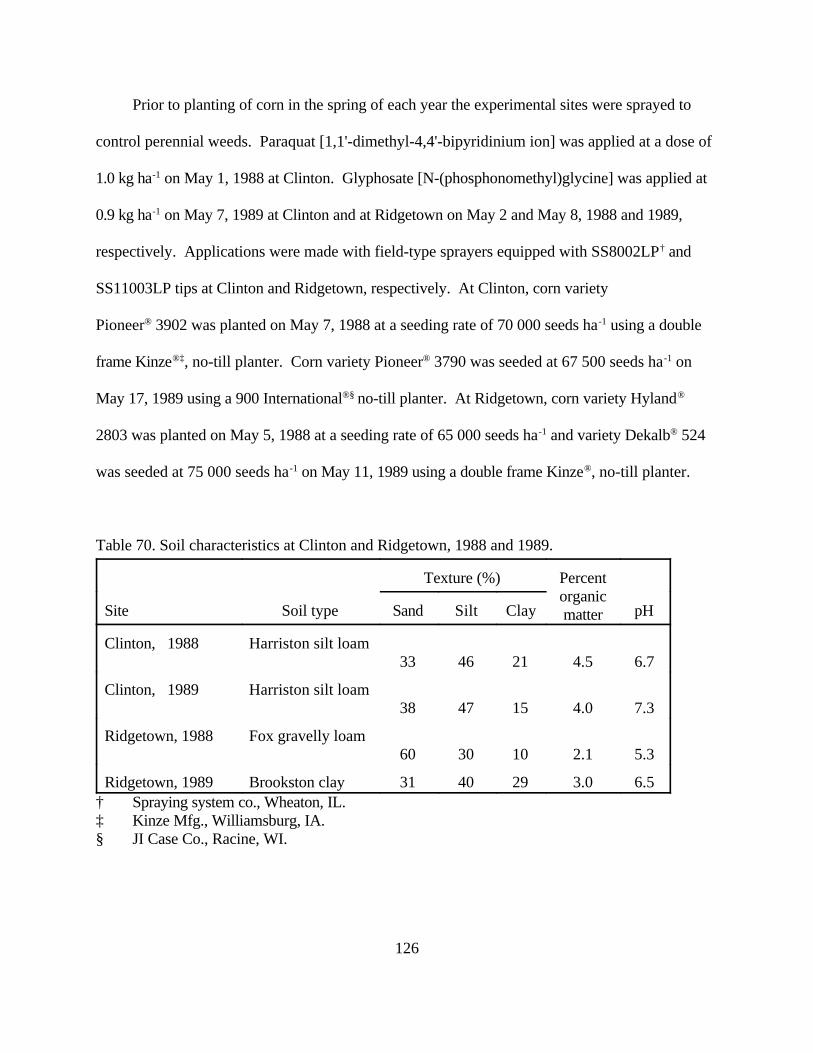
126
Prior to planting of corn in the spring of each year the experimental sites were sprayed to
control perennial weeds. Paraquat [1,1'-dimethyl-4,4'-bipyridinium ion] was applied at a dose of
1.0 kg ha-1 on May 1, 1988 at Clinton. Glyphosate [N-(phosphonomethyl)glycine] was applied at
0.9 kg ha-1 on May 7, 1989 at Clinton and at Ridgetown on May 2 and May 8, 1988 and 1989,
respectively. Applications were made with field-type sprayers equipped with SS8002LP† and
SS11003LP tips at Clinton and Ridgetown, respectively. At Clinton, corn variety
Pioneer® 3902 was planted on May 7, 1988 at a seeding rate of 70 000 seeds ha-1 using a double
frame Kinze®‡, no-till planter. Corn variety Pioneer® 3790 was seeded at 67 500 seeds ha-1 on
May 17, 1989 using a 900 International®§ no-till planter. At Ridgetown, corn variety Hyland®
2803 was planted on May 5, 1988 at a seeding rate of 65 000 seeds ha-1 and variety Dekalb® 524
was seeded at 75 000 seeds ha-1 on May 11, 1989 using a double frame Kinze®, no-till planter.
Table 70. Soil characteristics at Clinton and Ridgetown, 1988 and 1989.
Texture (%) PercentorganicmatterSite Soil type Sand Silt Clay pH
Clinton, 1988 Harriston silt loam33 46 21 4.5 6.7
Clinton, 1989 Harriston silt loam38 47 15 4.0 7.3
Ridgetown, 1988 Fox gravelly loam60 30 10 2.1 5.3
Ridgetown, 1989 Brookston clay 31 40 29 3.0 6.5† Spraying system co., Wheaton, IL.‡ Kinze Mfg., Williamsburg, IA.§ JI Case Co., Racine, WI.

127
Table 71. Mean and percent of normal precipitation accumulation by month at Clinton andRidgetown, 1988 and 1989.
Precipitation†
1988 1989
Month mmPercent ofnormal‡ mm
Percent ofnormal‡
Clinton
May 76.0 103 100.1 136
June 17.5 23 99.5 133
July 62.7 82 2.0 3
August 93.0 97 87.5 91
September 138.5 157 69.0 78
Ridgetown
May 45.3 67 132.6 197
June 15.0 19 89.0 115
July 65.8 91 35.0 48
August 78.5 99 90.1 113
September 74.5 108 49.2 71† Data from Canada, Dept. of Transport., Meteorological Branch.
1990. Meteorological Observations in Canada - Monthly Record.‡ 50 year average.
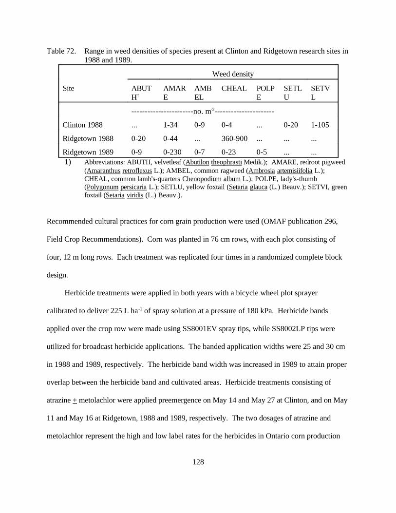
128
Table 72. Range in weed densities of species present at Clinton and Ridgetown research sites in1988 and 1989.
Weed density
Site ABUTH†
AMARE
AMBEL
CHEAL POLPE
SETLU
SETVL
-----------------------no. m-2----------------------
Clinton 1988 ... 1-34 0-9 0-4 ... 0-20 1-105
Ridgetown 1988 0-20 0-44 ... 360-900 ... ... ...
Ridgetown 1989 0-9 0-230 0-7 0-23 0-5 ... ...1) Abbreviations: ABUTH, velvetleaf (Abutilon theophrasti Medik.); AMARE, redroot pigweed
(Amaranthus retroflexus L.); AMBEL, common ragweed (Ambrosia artemisiifolia L.);CHEAL, common lamb's-quarters Chenopodium album L.); POLPE, lady's-thumb(Polygonum persicaria L.); SETLU, yellow foxtail (Setaria glauca (L.) Beauv.); SETVI, greenfoxtail (Setaria viridis (L.) Beauv.).
Recommended cultural practices for corn grain production were used (OMAF publication 296,
Field Crop Recommendations). Corn was planted in 76 cm rows, with each plot consisting of
four, 12 m long rows. Each treatment was replicated four times in a randomized complete block
design.
Herbicide treatments were applied in both years with a bicycle wheel plot sprayer
calibrated to deliver 225 L ha-1 of spray solution at a pressure of 180 kPa. Herbicide bands
applied over the crop row were made using SS8001EV spray tips, while SS8002LP tips were
utilized for broadcast herbicide applications. The banded application widths were 25 and 30 cm
in 1988 and 1989, respectively. The herbicide band width was increased in 1989 to attain proper
overlap between the herbicide band and cultivated areas. Herbicide treatments consisting of
atrazine + metolachlor were applied preemergence on May 14 and May 27 at Clinton, and on May
11 and May 16 at Ridgetown, 1988 and 1989, respectively. The two dosages of atrazine and
metolachlor represent the high and low label rates for the herbicides in Ontario corn production
129
(Ontario Weeds Committee, 1988). The weedy control had no herbicide applied or cultivation
and the weed-free control was hand weeded as weeds emerged.
Inter-row cultivations were performed using a Hiniker® (Hiniker Co., Mankato, MN.), 4-
row, sweep-type cultivator with the mid-points of the sweep teeth set to operate at a depth of 3 to
5 cm. The cultivator sweep teeth were increased in width from 45 cm in 1988 to 50 cm in 1989,
to achieve better overlap between the herbicide band and cultivated areas. Two inter-row
cultivations were performed at each research site with the timing corresponding to the 7 and 13
leaf stage of corn growth. A new leaf stage was determined to have been reached when the leaf
appeared in the corn whorl. The first inter-row cultivation was delayed until the 10 leaf stage of
the corn crop in 1989 due to rainfall. Cultivations occurred at Clinton and Ridgetown on June 13
and July 4 in 1988, and June 27 and July 6 in 1989, respectively.
Observations
Only corn grain yield from the 1989 Clinton site is presented, due to extremely low weed
populations. The results and discussion section will be focused on the three remaining research
locations.
Weed observations were taken from a 1.0 m2 quadrat centred over one of the middle rows in
each plot approximately 2 weeks after the second inter-row cultivation. Weed density by species
was recorded and the above ground biomass by species was clipped at the soil surface, oven dried
for 5 days at 800C, and dry weights recorded. This occurred at Clinton on July 18 in 1988, and at
Ridgetown on July 20 and July 13, in 1988 and 1989, respectively. Weed density and biomass

130
measurements were repeated at Clinton on September 12 in 1988, and at Ridgetown on September
21 and September 12, in 1988 and 1989, respectively. Weed density and biomass by species were
grouped into total broadleaf and total grass for presentation purposes.
Corn grain yield was determined by harvesting a 3.0 m length from the middle 2 rows of
each plot. Harvesting occurred on October 20, 1988 and October 16, 1989 at Clinton, and
October 15, 1988 and October 13, 1989 at Ridgetown. Corn ears were hand-picked, fresh weight
determined, dried for 7 days at 800C, weighed, shelled, and reweighed. Grain yield was calculated
based on 15.5% moisture content and expressed in kg ha-1.
Statistical Analysis
The experimental results were analyzed separately for each location and year of this study
due to a year by treatment interaction. Weed density and biomass data were subjected to square
root(x+1) and log10(x+0.5) transformations, respectively, to fit the data to a more normal
distribution. Treatment means were separated using transformed data and original data means
were used for presentation. Transformation was not necessary for corn grain yield data, therefore
original data was used for analysis. With the control treatments excluded, all data were subjected
to analyses of variance, and main effects and interactions were tested for significance. Orthogonal
comparisons were performed utilizing SAS (Statistical analysis system, SAS institute inc., Cary,
NC.) procedures to investigate significant interactions among main effects and linear contrasts of
treatment means were also performed.
131
RESULTS AND DISCUSSION
Corn grain yield and weed biomass and density measurements were analyzed and presented
in terms of herbicide application method, number of inter-row cultivations and herbicide
combination and dose required. After determining the best weed control treatment at each
research site, comparisons were made between that treatment and other individual treatments
utilizing linear contrasts.
Yields were low at the 1989 Ridgetown site because of seasonal drought conditions.
Annual weed densities and germination patterns varied at the individual research sites and
therefore required different herbicide and cultivation combinations to achieve adequate weed
control.
Herbicide Application Method
Corn grain yield did not differ significantly regardless of whether herbicides were applied
as a band or broadcast treatment at all four research sites (Tables 75, 76, 77). Previous work by
Moomaw and Martin (1978) found that when 2,4-D [(2,4-dichlorophenoxy)acetic acid] was
applied prior to planting, slot-planted corn yields were not significantly different between band or
broadcast preemergence herbicide treatments when used in combination with cultivation.
Banded treatments required cultivation as indicated by the cultivation by application
interaction which was significant for corn grain yield and total broadleaf weed biomass and
density at three of the four research sites, excluding the 1989 Clinton site, where weed pressure
was very low (Tables 73, 74, 77 and 78). This interaction was expected because herbicides

132
applied in a band combined with 0 cultivations resulted in lower corn yields and higher total
broadleaf weed biomass and density. For example, at Ridgetown in 1989, corn grain yields for
banded treatments combined respectively with 0, 1 and 2 cultivations, were 3610, 4830 and 4810
kg ha-1. A non orthogonal linear contrast was utilized to compare banded to broadcast herbicide
applications averaged over 1 and 2, and 0, 1 and 2 cultivations, respectively. Banded treatments
combined with 1 or 2 cultivations were equal to broadcast treatments except for broadleaf weed
control at Ridgetown in 1988 (Tables 75 and 79). Here, herbicides applied in bands had higher
total broadleaf weed biomass and density because of weed escapes which were due to a lack of
proper overlap between the herbicide band and cultivated areas. This demonstrated the need for
adequate overlap between the cultivated and herbicide banded areas, especially in a situation of
high weed density.
Cultivation
The number of cultivations in combination with banded herbicide treatments required to
maintain weed control and corn grain yield varied between sites. To determine the number of
cultivations required, orthogonal contrasts were made to compare between 0, 1 and 2 cultivations
within banded herbicide application treatments.
At Ridgetown in 1988 and 1989, a significant quadratic contrast revealed that banded
herbicide treatments combined with 1 cultivation was adequate to maintain corn grain yield
(Tables 77 and 78). Even though the first cultivation was delayed until the 10 leaf stage of the
corn crop in 1989 due to an extended period of rainfall, corn yield was not affected because there
was adequate moisture for both the weeds and corn, and the weed population was not excessive.

133
At the 1988 Clinton site, a significant linear contrast showed that two cultivations combined
with herbicides applied in bands resulted in significantly greater corn grain yield (Table 73).
Moomaw and Martin (1978) found that two cultivations rather than one tended to increase yields
of no-till corn. However, the planting and cultivating systems used in their study differed from
those used in our work. The extremely low weed population at the 1989 Clinton site resulted in
corn grain yields being equivalent across all treatments (Table 76). Cultivation had no significant
effect on corn grain yield in the absence of weeds.
To significantly reduce weed biomass and density in banded herbicide treatments,
cultivation was essential. Similar to corn grain yield, the number of cultivations required to
achieve adequate weed control varied between sites. In both years of experimentation, there was
little precipitation between the time of first cultivation and full canopy closure of the corn crop. In
a year where substantial rainfall after the first cultivation stimulated weed germination, a second
cultivation may be required.
At Clinton in 1988, two cultivations combined with herbicides applied in bands resulted in
significantly lower weed biomass and density (Tables 73 and 74). Later germinating annual grass
and broadleaf weeds were controlled by the second cultivation.
At Ridgetown in 1988 and 1989, one cultivation combined with banded herbicide treatments
was adequate to maintain weed control (Tables 77 and 78). The exception to this was in 1988
when two cultivations resulted in lower broadleaf weed biomass in September. Weed escapes
did occur in treatments containing one cultivation, however corn grain yield was not affected.
Generally part these weed escapes could be attributed to the lack of overlap between the herbicide
band and cultivated areas which was experienced in 1988. The presence of these weeds could
present a problem with respect to contribution to the soil seed bank. However, weed seeds
134
dropping on the soil surface may not be as much of a problem in Ontario no-till conditions because
of seed viability loss over the winter months. Typically seed decline is more rapid following
shallow rather than deep burial (Froud-Williams 1987). For example, Thomas et al. (1986)
showed that less than 1% of green foxtail seed sown on the soil surface was viable after six years,
whereas buried seeds remained viable up to 17 years.
Non orthogonal, linear contrasts were performed to evaluate the weed control efficacy of
cultivation alone without a herbicide treatment present. Comparisons were drawn between the
treatment containing the optimal banded herbicide application and cultivation combination, and the
control treatments containing one and two cultivations, treatments twenty and twenty one,
respectively. At both sites in 1988, cultivation alone did not adequately control weeds (Tables 75
and 79). Significantly higher levels of weed control and corn grain yields were recorded for
treatments containing herbicides applied in a band plus cultivation. At the 1989 Ridgetown site,
significantly greater weed control was achieved where the treatment contained a banded herbicide
application, although final corn grain yield did not differ significantly from the cultivation alone
treatments (Table 79).
Herbicide Combination and Dose
Atrazine or tank-mixtures of atrazine + metolachlor applied at high and low label dosages
were evaluated in terms of weed control and corn grain yield. At Clinton in 1988 and 1989 and
Ridgetown in 1989 weed control and corn grain yield did not differ significantly regardless of the
herbicide combination or dosage of herbicide applied.

135
At the 1988 Clinton site, corn grain yield and total broadleaf weed biomass and density
were equivalent regardless of the herbicide combination or dosage of herbicide applied (Tables
73 and 74). However, total grass biomass and density was significantly reduced when
metolachlor was included. This annual grass pressure did not reduce corn grain yield but
contribution to the soil seed bank remains a possible problem.
At Ridgetown in 1988, corn grain yields were significantly higher and total broadleaf weed
measurements taken in July were significantly lower, where the high label rates of atrazine and
metolachlor were used (Table 77). Non orthogonal linear contrasts comparing herbicide
treatments within banded herbicide applications indicated similar results. In cases of high weed
densities as was found at this site, high rates of herbicides applied in a band may be required to
achieve weed control because of the potential for herbicide dilution out of the band due to lateral
movement in the soil. At the 1989 Ridgetown site, atrazine alone applied at the low label rate was
a sufficient herbicide treatment to maintain weed control and corn grain yield (Table 78). Annual
grass pressure at this site was minimal.
Herbicides applied in banded applications combined with inter-row cultivation can provide
adequate weed control and corn grain yields in a no-till production system. The herbicide
combination and use rates required in the banded applications, and the number of cultivations will
be specific to each grower's situation. Varying factors will include weed species, density and
emergence patterns as influenced by precipitation, efficacy of the herbicide and cultivation
treatments and management level of the grower.
For growers adopting the banded herbicide application and inter-row cultivation system, a
minimum herbicide band width of 30 cm and maintaining high label dosage is recommended.
Dilution of the herbicide band could arise through lateral herbicide movement in the soil or

136
variations in the boom height when applying the herbicide band. After experience with the new
system is gained, herbicide dosage and possibly the width of the band may be reduced in order to
minimize herbicide use.
Application of herbicides in 30 cm bands on 76 cm wide corn rows represents an
approximate 60% reduction of herbicide application into the environment and an immediate
economical savings for the no-till corn producer. As well, it is possible that corn yields may
benefit from lower herbicide use achieved through banded applications. Each herbicide
represents a physiological stress with respect to energy used by the crop plant for metabolism of
the herbicide. As corn roots grow out of the herbicide banded area, the plants may well be less
stressed. Another possible benefit of banded herbicide applications in no-till crop production is a
reduced chance of herbicides gaining entry into ground water or surface water runoff†. (Personal
communication. T.J. Vyn, Assoc. Prof., Dept. Crop Sci., Univ. of Guelph, Ontario, N1G 2W1.)
Kenimer et al. (1987) found that under no-till conditions, atrazine and 2,4-D [(2,4-
dichlorophenoxy)acetic acid] losses in surface water runoff were 0.3 and 0.02%, respectively, of
applied amount. These losses would have been even less if the herbicides had been applied in a
band.
Herbicide use for annual weed control in no-till corn production would be quite minimal if
conditions such as were found at the 1989 Clinton site were more prevalent. Besides the
application of glyphosate to control perennial and early-germinating annual weeds, no other weed
control method was required. The low annual weed pressure at this site can be attributed chiefly
to two factors: good management of a no-till cropping system for five years which probably

155
decreased the number of viable weed seeds in the germination zone near the soil surface and
effective use of glyphosate to control the early flush of annual weed seedlings.
The integration of banded herbicide applications, inter-row cultivation, and reduced
herbicide dosage represents a viable cropping alternative that integrates optimal herbicide use
with the environmental benefits of no-till.
6.6 RECOMMENDATIONS
On the basis of field experiments conducted at various sites from 1987 to 1990 the
following recommendations are suggested for the integrated weed management in corn and use of
2,4-D in soybeans in no-till crop management systems.
6.6.1 Tillage 2000: Preemergence Herbicides for Annual Weed Control in Various TillageSystems
! Currently registered herbicides at labelled rates provide similar weed control in all tillage
systems (no-till, ridge tillage, chisel or moldboard plough).
! There is no justification for increasing herbicide dosages in any given tillage system in corn.

156
6.6.2 Quackgrass Control in No-till Corn
! Under no-till system 82% of quackgrass rhizomes were found within top 7.5 cm of soil
surface.
! Apply glyphosate at 0.9 kg.ha-1 in the spring to actively growing quackgrass in the 3 to 5
leaf stage of growth.
6.6.3 Residual Effect of 2,4-D on the Soybeans
! Apply 2,4-D ester or amine formulation at 0.5 to 1.5 kg.ha-1 two weeks prior to soybean
planting or apply 2,4-D ester formulation only, one week prior to soybean planting.

157
OBJECTIVE # 7
7.0 TO STUDY THE COST/BENEFIT RATIO STRATEGIES UNDER NO-
TILL CROPPING SYSTEMS

158
7.1 ECONOMIC COMPARISON OF ALTERNATIVE TILLAGESYSTEMS UNDER RISK
Alfons Weersink
Michael Walker
Clarence Swanton
and
Jim Shaw
First Submission
Canadian Journal of Agricultural Economics
May 1991
The authors are respectively an assistant professor and a former graduate research assistant, Department of AgriculturalEconomics and Business, University of Guelph, an associate professor, Department of Crop Science, University ofGuelph and weed biologist, Ridgetown College of Agricultural Technology. The authors wish to thank Glenn Fox andCal Turvey for their helpful comments. Financial support for the project was provided in part by the Ontario Ministryof Agriculture and Food's Tillage 2000 project and the Agriculture Canada/NSERC Research Partnership Program andAgriculture Canada Soil, Water Environmental Enhancement Program (SWEEP).

159
ECONOMIC COMPARISON OF ALTERNATIVE TILLAGE SYSTEMS UNDER RISK
INTRODUCTION
The adoption of conservation tillage techniques have been widely recommended as a remedy
for the problem of soil erosion (Brady, 1984). By improving water quality, recreational value and
drainage of the surrounding streams and lakes through its reduction in soil loss, the use of conservation
tillage techniques can provide a net total benefit to society (Clark et al. 1985, Fox and Dickson 1990).
However, these off-farm benefits may be incurred at increased costs to farmers from increased
herbicide usage or from incremental machinery investment. Business and financial risk may also
increase if the new production system increases yield variability.
Previous studies which have compared the profitability of alternative tillage systems in Ontario
include Baffoe et al. 1987, Henderson and Stonehouse 1988, Stonehouse et al. 1987, Zantinge et al.
1986. The general conclusion of these studies is that conventional tillage is more profitable than
conservation tillage systems in producing monoculture corn. Studies comparing the net returns of corn
and soybeans cropping systems have been conducted for American conditions (Doster et al. 1983,
Duffy and Hawthorn 1984, Klemme 1983) and have generally concluded that the farm level economic
feasibility conservation tillage systems depends largely on the managerial skills necessary to produce
yields comparable to conventional tillage systems. However, these studies have not incorporated
yield variability and the associated riskiness involved with each tillage system which may play a
major role in determining the most efficient system for an individual producer (Fox et al. 1991).
Several studies in the U.S. Corn Belt (Klemme, 1985) and Great Plains (Mikesell et al. 1989,
Williams 1988) have assessed the income-risk trade-off from different tillage systems and concluded
that conservation tillage methods would be preferred by risk averse farmers. This conclusion,

160
however, may not be appropriate to Ontario since the importance of soil moisture retention in the High
Plains region may give conservation tillage a comparative advantage over conventional tillage.
The purpose of this study is to compare the production costs and income risk of three
conservation tillage systems; chisel plough, ridge till and no till, with a conventional moldboard
plough tillage system for a southern Ontario corn and soybean cash crop farm under alternative
scenarios. The next section of the paper defines the alternative farm scenarios which are distinguished
on the basis of size and soil type. The minimum costs for each scenario and tillage system are then
developed in consideration of timeliness restrictions, machinery complement size and other relevant
crop production data. The method of generalized stochastic dominance used to carry out the analysis
of income risk is then described. The comparison of production costs and income risk is then
presented followed by implications of the results for public policy.
METHODS
Net Farm Returns
Case Farm Scenarios
The field operations carried out under each of the four tillage systems to be examined in this
study are summarized in Table 80. Conventional tillage is defined by Christensen and Magleby
(1983) as a tillage system where 100 percent of the topsoil is mixed or inverted by ploughing. It
involves two stages with primary tillage breaking up the soil and burying the crop residue with a
moldboard plough. The second stage of secondary tillage produces a fine seedbed by further breaking

161
down soil particles by a series of passes using implements such as disks or cultivators. The chisel
plough tillage system is similar to the conventional system but it replaces the fall moldboard plough
with a chisel plough cultivator and completes the initial secondary field operation with a heavier
cultivator. However, it can be classified as a conservation tillage system since at least 30 percent of
the previous year's crop residue is on the soil surface after planting.
In ridge-till and no till systems, there is no pre-plant cultivation. Before planting, ridge-till and
no-till fields are sprayed with a contact herbicide. In ridge tillage, a conventional planter used in the
previous two systems is modified with sweeps and disk openers. During planting, the top few inches
of soil from each ridge are removed and the residue pushed aside to expose a raised seedbed. The
ridge is maintained during the growing season by inter-row crop cultivation so that the post-planting
operations are similar to the moldboard plough and chisel plough tillage systems. The only soil
manipulation required in the no-till system is the opening of a slit wide enough to receive a seed which
is then covered and packed with soil. In contrast to the ridge-till system, no inter-row cultivation is
done under a no-till system.
The net farm returns for each of the four tillage systems on a southern Ontario corn and soybean
farm are to be compared for six alternative farm scenarios established on the basis of farm size and
soil type for each tillage system. Farm sizes were split into three groups of 80, 160 and 240 hectares
in order to account for differing timeliness restrictions encountered for each size of farm and the
associated effect this will have on the sizing of machinery complements. In addition, two soil types,
clay-loam and sand, are also used to define alternative case farm scenarios since the different soil
types will affect available field work days and the yield performance of the tillage systems. Thus, 24
farm scenarios are to be considered; 4 tillage systems, 3 farm sizes and 2 soil types.

162
Machinery Complement
Each of the four tillage systems described previously requires a unique machinery complement
to complete the required field operations for each particular case farm scenario. The machinery
complement must match the tractor size with the required machine widths for each field operation and
enable the farmer to finish these operations efficiently within the critical time periods. The first step
is determining the time available to complete the field operations. The total amount of time for each
seven day period was estimated by multiplying the available field work days (OMAF Agdex 8ll,
1988) by the work hours per day. Within this time period, the field operations must be completed to
ensure there is no loss in maximum yield. The size of each implement can then be determined using
a procedure outlined in Kay (1986) which depends on the speed and field efficiency of the machine
and the rate at which the operation must be completed as determined by farm size and total working
time available. Tractor size was then matched to the power requirements of the implement.
Minimum Cost Structure
With the identification of the optimal machinery complement, the costs of owning that machinery
can be determined. The machinery fixed costs consist of an annual depreciation value, an interest on
investment and a value for insurance and housing. Annual depreciation was calculated on a declining
balance method with a 20% rate for combines, a 15% rate for tractors and a 10% rate for non-
powered machines. All equipment was assumed to be 5 years old with the current values obtained
by using the above depreciation rates on the present list prices for the equipment. The investment cost
on machinery was calculated as a weighted average cost of capital multiplied by the average life time
market value of the equipment. Machinery insurance and housing was assumed to be based on 1.5%

163
of the purchase price. A land rental charge and general overhead expense was also charged equally
for all tillage systems.
Variable input costs for seed, fertilizer and harvesting were assumed to be the same across all
tillage systems. The variable machinery costs for repairs and fuel depend on the hours of use, tractor
size and the type of field operation which vary under the alternative scenarios. These factors will also
influence the total amount of labour used which was valued at $8 per hour. Herbicide costs for each
tillage system were based on the optimum treatment for each system.
Prices and Yields
The final element necessary to calculate net farm returns for each farm scenario is gross
revenue. Prices for corn and soybeans were the 1983-1989 average converted into 1989 day dollars.
Paired yield data for corn and soybean crops grown in rotation were collected from seventeen farms
throughout southern Ontario over a four year period from 1986-1989. Repeated yield observations
were measured at different areas within each field. Supplementary yield data was collected from
several other farms where the yield observations for the relevant tillage system and soil type were
sparse.
The summary statistics for actual farm yield data under the four different tillage systems for corn
and soybeans are given in Table 81. Normality of yield distributions was rejected using the Shapiro-
Wilk test statistic for all scenarios with the exception of soybean yields on sandy soils and moldboard
plough tillage. A non-parametric approach was therefore necessary to analyze the yield data. The
results of the Wilcoxon Rank Sum Test indicated there was no difference in tillage system population
locations for corn yields at the 5 percent significance level with the exception of the moldboard plough
- chisel plough comparison on clay loam soils. On clay soils, soybean yields with no-till were
164
significantly lower than either moldboard or chisel plough tillage system yield populations. On sandy
soils, the soybean yields for these two fall tillage systems were significantly lower than ridge till. The
results of the Moses dispersion test comparing the ratio of scale parameters between tillage system
and yield population suggested that there is less variability between tillage systems on sandy soils than
clay loam soils.
Stochastic Dominance
Due to the variability in yields under alternative tillage systems, there is a probability
distribution associated with net returns for each farm scenario. The tillage system which maximizes
producer utility from uncertain returns under alternative risk attitudes is determined using stochastic
dominance. Stochastic dominance is an analytical technique which enables the ranking of two
cumulative distributions for different classes of risk preferences when neither the utility function or
risk aversion parameters are known. It is a more flexible approach to risk analysis than alternatives
such as EV and MOTAD which assume constant absolute risk aversion decision makers and normal
outcome distributions. Cochran (1986) reviewed comparisons of different risk analysis techniques and
concluded that stochastic dominance is the most accurate when non-normal return distributions are
being compared. The distribution of the yield data used in this study has just been shown to be non-
normal which is generally the case for agricultural crop yields (Day, 1965) and for net farm returns
based on price-yield values (Buccola,1986).
There are several stochastic dominance efficiency criteria distinguished largely by the risk
preference interval†. The ordering of choices can then be achieved for the specific group of decision
makers defined by the imposed restrictions on the risk preferences by elimination of the choices which
do not conform to the restrictions. The remaining choices are part of the efficient set which contains

165
the preferred choice of all the decision makers whose preferences are represented by the restrictions
imposed by the efficiency criterion (Levy and Sarnat, 1972).
First degree stochastic dominance(FSD) ranks alternative choices such that if x is an outcome
measure, such as net farm returns, a decision maker will always prefer more of x to less regardless
of their risk preferences. Graphically, the FSD criterion can be defined where dominance (greater
expected utility) is shown when the two cumulative probability density functions (CDF) never cross
and the dominant CDF, lies to the right of the dominated CDF (King and Robison, 1984). The FSD
criterion has very low discriminatory power, since it includes all decision makers who prefer more
to less, and this results in large efficient sets, with few eliminated choices.
______________________________________________________________________________
† The alternative stochastic dominance efficiency criteria are reviewed by Cochran, Robinson
and Lodwick (1985).
In addition to the assumption of a monotonically increasing utility function for the decision
maker, second degree stochastic dominance (SSD) imposes the additional restriction that the utility
function be strictly concave at all outcome levels. The assumption that the decision maker is averse
to risk makes SSD more discriminating than FSD. Graphically, under second degree stochastic
dominance the CDF's are now compared by the accumulated area under each distribution function.
While SSD is more discriminatory than FSD it may still produce large efficient sets. The inclusion
of decision makers with a maxi-min attitude† can increase the size of efficient sets due to the left hand
tail problem. This results in a disproportionate weighting of the lower values of some cumulative
density functions such that they cannot be excluded from the SSD efficient set.

166
r(x) '&u ))(x)
u )(x)
Generalised stochastic dominance (GSD) developed by Meyer (1977), is more discriminatory than
FSD and SSD, and is more flexible in defining individuals preferences. GSD is expressed formally
by King and Robison (1984) as the necessary and sufficient conditions under which the CDF F(x), of
a function f, is preferred to the CDF G(x), of a function g, by all individuals whose absolute risk
aversion functions lie everywhere between specified lower and upper bounds, r1(x) and r2(x). The
absolute risk aversion function (Arrow 1971, Pratt 1964) is defined as
where ut(x) and u"(x) are the first and second derivatives of a monotonically
______________________________________________________________________________†
This is a decision maker who concentrates on the worst possible outcome for each choice, and
selects action that maximises the minimum gain.y
increasing von Neumann-Morgenstern utility function U(x). These give a unique measure of
preferences and are unaffected by arbitrary transformations of the utility function. The sign indicates
risk aversion (positive), risk neutrality (zero), or risk preference (negative), and they enable
interpersonal comparisons of risk aversion to be made at different outcome levels. A particular value
of r(x) can be identified as the percent reduction in marginal utility per unit of x, for example if x is
measured in dollars, a value of r(x) = 0.0002 indicates that marginal utility is dropping at the rate of
0.02% per dollar.
GSD allows the classes of decision makers to be identified by specifying the preference interval
of their utility functions, which are bounded by lower, r1(x), and upper, r2(x) absolute risk aversion

167
Maximize m1
0[F(x)&G(x)] u )(x)dx (2)
r1(x)ò &u ))(x)
u )(x)ò r2(x) (3)
coefficients. FSD and SSD are restrictive cases of the GSD model. FSD has a large interval width
with no restriction on the decision makers absolute risk aversion coefficients, such that r1(x) = -4 and
r2(x) = 4 for all values of x. SSD restricts the decision makers marginal utility to be positive, which
implies r1(x) = 0 and r2(x) = 4 for all values of x.
Meyer (1977) set up an optimal solution procedure for Generalised Stochastic Dominance with the
Arrow-Pratt absolute risk aversion coefficient as the control variable. The problem is defined as
follows;
subject to the constraint
for all values of x, and the initial condition ut(0) = 1. Equation (1) accounts for the difference between the expected utilities of CDF's F(x) and G(x),
which represent outcome distributions f and g respectively. If for a given class of decision makers,
defined by equation (2), the maximum of this difference is negative, then f dominates g by GSD for all
r(x) between r1(x) and r2(x). GSD, unlike FSD and SSD, places no restrictions on the absolute risk
aversion coefficients, r(x) is constrained to lie between r1(x) and r2(x), but there may be increasing,
decreasing, or oscillating risk aversion utility functions within these bounds.
Accurate estimation of the risk aversion coefficient (RAC) intervals relative to the outcome
variable, when the decision makers risk preferences are unknown, has been identified as being of
critical importance by McCarl (1990). Calculation of the upper RAC bound from the relationship
between the risk premium, expected income level and the certainty equivalent when wealth is ignored,

168
has been suggested by McCarl and Bessler (1989). They also give examples of other studies which
have incorrectly specified the RAC intervals, resulting in inaccurate classification of risk preferences.
Net farm returns per hectare were multiplied directly by farm size such that proper transformations
of scale of the outcome distributions maintained correct ranking by GSD (Raskin and Cochran, 1986).
EMPIRICAL RESULTS
Net Returns Analysis
Corn and soybean yields are multiplied by their 1983-1989 average real price to obtain gross
revenues. The revenues are reduced by variable and fixed production costs for each farm scenario
to arrive at net returns. The returns on any farm size is the average of corn and soybean net returns
which are assumed to be planted in equal proportions. The gross revenues, production costs and net
returns to management for each of the 24 case farm scenarios are summarized in Table 82.
Analysis of the gross revenues for alternative tillage systems parallel the relative performance
of their yields discussed previously. The variable costs for ridge-till and no-till are higher than the
two fall tillage systems due to higher chemical weed control costs. However, machinery costs for the
moldboard and chisel plough tillage systems are approximately double that for the other two systems.
The higher fixed costs offsets the lower variable costs sufficiently to result in greater total production
costs for the moldboard and chisel plough tillage systems. For all four tillage systems, production
costs per hectare increase moving from the 80 hectare farm size to the 160 hectare due to the use of
a custom combine operator for the smaller farm scenario versus the ownership of a combine for the
larger farm sizes. Per hectare costs then fall when moving to the 240 hectare farm size due to
economies of size in machinery. There is little difference in total costs per hectare between clay and

169
sandy soils due to a "lumpiness" effect in machinery sizing. As a result, a similar complement is
chosen for both soil types even though the time constraint is less critical on sandy soils.
Given that ridge-till was generally the dominant tillage system in the majority of paired yield
comparisons and its relatively low cost structure, it should be expected that mean net returns are
highest for the ridge-till system in all farm scenarios. To verify the differences between net returns of
the alternative tillage systems, the non parametric Wilcoxon Rank Sum Test was used to compare
paired population locations since the Shapiro-Wilk Test rejected the assumption of normality in the
net farm returns distribution for any of the farm scenarios. On clay soils, the net return distribution
is significantly different from the ridge till net return distributions for all farm sizes. The moldboard
plough tillage system compared favourably at the smaller farm size but its net return location is
significantly less than ridge till at the 240 hectare farm scenario due to changing machinery investment
costs. On sandy soils, the relative performance of average net returns improves for no till and ridge
till compared to the two fall tillage systems. The moldboard and chisel plough tillage systems have
significantly lower population locations from ridge-till for all farm sizes on sandy soils.
The Shorack Ratio Estimator was used to rank the variability in net returns of the four
alternative tillage systems. On clay soils, the fall tillage systems of moldboard and chisel plough had
the lowest net return variability followed by no-till and ridge-till. These rankings were reversed for
the sandy soil farm scenarios.
GSD Analysis of Tillage System Net Farm Returns.
The empirical net farm return distributions differ across the alternative farm scenarios. In order
to select the most efficient tillage system under different farm conditions and risk attitudes of the
operator, stochastic dominance risk assessment techniques are utilized.

170
r2(x) ò 2CV ( SD
The computer program Meyeroot developed by McCarl (1989), was used to rank the net farm return
distributions for each of the four tillage systems at each farm scenario. This is a modified version of
the Meyer (1975) optimal control algorithm for GSD, which ranks pair wise comparisons of
cumulative density functions (CDF) when the upper and lower risk aversion coefficients (RAC) are
specified. The Meyeroot program searches upward from the lower bound, and downward from the
upper bound for any break-even risk aversion coefficient values, where dominance between tillage
systems changes. The correct selection of upper and lower bounds relative to the scale of the outcome
distribution was recognised to be an important factor in successfully running the program.
The non-negative certainty equivalent method of McCarl and Bessler (1989) was used to set
approximate upper bounds for the RAC, r2(x), for each of the six case farm scenarios being
considered. The upper bound value was calculated from the following equation using values of
coefficient of variance (CV) and standard deviation (SD) from Table 82;
Pair wise comparisons of each tillage system were then carried out for incremental levels of the
RAC range, to identify any multiple changes in dominance between the upper and lower RAC bounds.
The Meyeroot program identified break-even risk aversion coefficient (BRAC) values where
dominance changed between pairs of tillage systems and it was then possible to rank the tillage
systems for each incremental risk interval within the overall RAC bounds. Tillage systems dominant
in the negative risk aversion range would be preferred by risk preferring individuals. Likewise
dominant tillage systems in the positive risk aversion range would be preferred by risk averse
producers, with the largest positive RAC value representing the most risk averse producer.

171
The results of the GSD rankings for each farm scenario are illustrated below in Table 83. The
break-even risk aversion coefficients (BRAC), which represent the RAC values where dominance
changes between tillage systems are also given. Ridge-till systems dominate in almost every risk
interval and across all farm scenarios, with the exception of the moldboard plough system which
dominates in several of the slightly risk averse intervals for clay loam soil type farms.
For all three clay loam scenarios risk preferring and strongly risk averse individuals have the
same preference of ridge-till, while moderately risk averse producers prefer moldboard plough
tillage. This phenomena is partially explained by Grube (1986), where he notes that from game
theory, the most risk preferring strategy would be chosen by a maxi-max individual and the most risk
averse strategy by a maxi-min individual. This could result in distributions with lower minimums and
higher maximums being preferred by both risk averse individuals and risk preferring individuals.
Ridge-till does not have lower minimum net returns than moldboard plough, therefore the study by
McCarl (1988) might better explain this result of alternating dominance. It was noted that the
empirical distribution functions may cross several times due to the empirical data source, resulting
in several changes in dominance. He also found that the utility difference approaches zero as the RAC
value approaches both zero and positive infinity, for any paired comparison.
The no-till system on clay loam soils is ranked second by risk preferring and fourth by risk
averse individuals. In contrast, the moldboard plough and chisel plough systems are least favoured
by risk preferring individuals and more favoured by risk averters. This result concurs with the net farm
return data in Table 82, where the mean net return levels are higher for the moldboard plough and
chisel plough systems, yet the maximum value is highest for no-till, and would therefore be chosen by
risk preferring individuals.
172
The moldboard plough system is preferred for three risk averse intervals over ridge-till for the
80 hectare clay loam soil farm. This decreases to only one risk aversion interval for the 240 hectare
farm size and may be explained by larger increases in both the mean and standard deviation for ridge-
till over moldboard plough as farm size increases for clay loam soil types.
The sandy soil GSD tillage rankings are more concise with almost equal rankings for each risk
aversion interval and farm size. The ridge-till and no-till systems outrank the two fall tillage systems,
indicating the advantage of reduced tillage systems on sandy soil types. Moldboard plough systems
would be preferred to chisel plough systems for 80 hectare farm sizes, but risk averse individuals
would prefer chisel plough to moldboard plough for the 160 and 240 hectare farm sizes.
Sensitivity of the Moldboard Plough and No-Till Comparison on Clay Loam Soils.
A sensitivity analysis was undertaken to illustrate the effect of parallel shifts in a tillage system
location, and the effect on the producers risk attitudes for moldboard plough and no-till systems on
clay loam soils. These two particular systems were chosen to enable a good comparison between
conventional tillage and a common conservation tillage system. Also the relatively large data sets
should provide a realistic representation for each system and a solid data base from which to draw
any conclusions.
Increasing parallel population location shifts were applied to the 160 hectare clay loam no-till
system, and repeated GSD comparisons with the moldboard plough system were carried out. The
resulting changes in break-even risk aversion coefficients are charted relative to the no-till population
location shift (Figure 1). These represent the RAC value at which dominance changes from no-till to
the moldboard plough system.

173
As the no-till population location is increased, then the BRAC values increase, which results in the
no-till system becoming dominant in the positive risk aversion space of the RAC bound, or it becomes
relatively more favourable to risk averse producers. There is risk neutrality between +$4000 and
+$6750 net returns per farm population location shifts of no-till, which indicates that risk neutral
individuals would be indifferent between tillage systems in this range. The additional monetary value
necessary to make no-till dominant to moldboard plough for risk averse producers is $6750. This is
equivalent to a net farm return increase of $40 per hectare (from $102 ha-1 to $142 ha-1), which equates
to a 625 kg.ha-1 increase in average corn yield alone (8575 to 9200 kg.ha-1), or a 300 kg.ha-1 increase
in average soybean yield alone (2725 to 3025 kg.ha-1), or some combination of both. The higher
variability of net returns of the no-till system means that the mean net returns per hectare has to be
higher, at $142 ha-1, than the moldboard plough mean net return at $ 128 ha-1, before the no-till system
is preferred by a risk averse producer. This yield difference would be less for the chisel plough
system to dominate the moldboard plough system, as it is ranked above the no-till system in the risk
neutral and risk averse intervals for this particular farm scenario.
This sensitivity analysis indicates that no-till conservation tillage systems have the potential to
produce higher levels of net returns, however the associated high levels of net return variability make
them unattractive to risk averse producers. The rate farmers adoption levels and possible government
policy implications for conservation tillage systems based on this particular comparison will depend
on the individual risk attitudes of the agricultural producers. Farmers with maximin or maximax
attitudes would be represented in the risk preferring interval and would require minimal incentive,
if any, to adopt the no-till system. More risk averse producers would need larger financial incentives
or improved production techniques before converting from conventional to conservation tillage
systems.

174
A comparison between the ridge-till and moldboard plough systems would most likely produce
opposite results from above, with ridge-till system appearing more favourable to almost all producers.
Qualifying this result, by allowing for the limited data source for ridge-till, then it illustrates the fact
that it is possible for conservation tillage systems to be preferred to the conventional moldboard
plough system under good management production techniques. On a more practical note, resulting from
personal communications with conservation tillage specialists, it is noted that the adoption of ridge-till
systems is presently declining due to the difficulty in achieving consistently high soybean yields with
the wide row spacing required for ridge-till systems. The results for this particular system can
therefore be viewed with slightly less relevance than for the other two conservation tillage systems
being considered.
CONCLUSIONS
This study has attempted to define and utilise stochastic dominance efficiency criteria to rank the
net farm return distributions for four different tillage systems under six different farm scenarios. Upper
and lower risk aversion coefficient (RAC) bounds were identified for each farm scenario based on
the size and spread of the outcome distributions. The Meyeroot computer program was then used to
carry out pair wise comparisons of tillage systems over each incremental RAC bound to identify
regions where dominance may switch between tillage systems. It was then possible to rank the tillage
systems relative to the risk preference interval within the overall RAC bounds.
Ridge-till systems were generally the dominant tillage system for all farm scenarios considered,
however, the limited source of ridge-till yield data may unfairly weight this particular system. No-till
systems on clay loam soils were more dominant in the risk preferring range and less dominant in the

175
risk averse range, which relates to the relatively larger range of net return values and smaller mean
net return values generated by this tillage system. Conversely, the moldboard plough and chisel plough
systems were more dominant in risk aversion intervals and less dominant in the risk preferring
intervals for clay loam soils. In sandy soil scenarios the ridge-till and no-till systems were dominant
over the two fall tillage systems for all farm sizes indicating that these tillage systems are more
competitive with conventional tillage systems in lighter soil type situations.
A sensitivity analysis between moldboard plough and no-till systems indicated that no-till would
dominate in risk preferring intervals, and an increase in no-till net farm returns of $40 per hectare
would change dominance in favour of no-till in risk averse interval space. By further considering a
comparison of the ridge-till and moldboard plough systems, it is evident that it is possible for
conservation tillage systems to dominate conventional tillage systems for almost all individual's risk
intervals, if proper agricultural crop production techniques are undertaken.

182
MINIMUM COSTS OF ALTERNATIVE TILLAGESYSTEMS
by
Alfons Weersink
Michael Walker
Clarence Swanton
and
James E. Shaw
1st Submission
Journal of Soil and Water Conservation
April 1991
The authors are respectively an assistant professor, a former graduate research assistant in the Department of
Agricultural Economics and Business, an associate professor in the Department of Crop Science, University of
Guelph and weed biologist, Ridgetown College of Agricultural Technology, Ontario Ministry of Agriculture and
Food.
Funding was provided by the Technology Evaluation Program (TED) as part of the Soil and Water Environmental
Enhancement Program (SWEEP) and the Agriculture Canada/NSERC Research Partnership Program.

183
7.2 MINIMUM COSTS OF ALTERNATIVE TILLAGE SYSTEMS
INTRODUCTION
Conservation tillage offers the potential for reducing the level of soil erosion and may
therefore lead to an improvement in the recreational value and drainage of surrounding lakes and
streams, a reduction in water treatment costs, and an improvement in water quality. These off-farm
benefits to society may, however, be incurred at the expense of the individual producer in the form
of higher production costs and reduced yields. The costs associated with conservation tillage stem
from a reduction in the efficiency of machinery use and a potential increase in herbicide costs to
ensure good weed control (Brady, 1989). These costs are offset by lower production costs
stemming from fewer tillage operations and a smaller investment in machinery. Many studies on
the profitability of alternative tillage systems have examined the cost trade offs but the costs for
each system are often derived from actual farm records or constructed for an average farm in the
study location. Either way, the costs will not likely represent the minimum levels possible for
each system and thus may not be appropriate for comparison.
The purpose of this paper is to derive the minimum costs associated with three conservation
tillage systems, chisel plough, ridge-till and no-till, and a conventional moldboard plough tillage
system for hypothetical corn-soybean farms in southern Ontario differentiated by farm size and soil
type. Since the trade offs in costs between alternative tillage systems deal largely with machinery
and herbicides, specific emphasis will be placed on these two cost items. Machinery costs will
be derived for the equipment base which will just enable the producer to complete field operations
within the critical time periods without suffering yield losses while the optional pre-emergent
herbicide for corn and soybeans is identified from a range of different applications for each crop.

184
METHODS
Case Farm Scenarios
The four tillage systems involved are a conventional tillage system using a moldboard
plough and three conservation tillage systems: chisel plough, ridge till, and no-till systems. In
general, ridge-till and no-till substitute the use of herbicides for fall and spring tillage operations
and plant directly into the previous year's crop residue. The chisel plough cultivation system
replaces the fall moldboard plough with a chisel plough cultivation. It can be classified as a
conservation tillage system since at least 30 percent of the previous years crop residue remains on
the soil surface after planting.
Six farm situations were defined using the variables of farm size and soil type to represent the
different types of cash crop farms in Southern Ontario. Farm sizes were split into three groups of
80, 160, and 240 hectares. By choosing three different farm sizes, it is possible to take account of
differing timeliness restrictions and the associated effect on the sizing of machinery complements
which will be encountered for each size of farm. The two crops being studied, corn and soybeans,
will be grown in rotation with each farm growing equal hectarage of both crops. Farms are also
distinguished by soil type, clay or sandy, since changes in soil type will have a dramatic effect on
the soil workability and the number of available field work days in the growing season. Thus, the
four tillage systems will be evaluated for each of the six farm scenarios, three farm sizes, and two
soil types, resulting in twenty four farm situation input cost structures to be considered. This
should provide a wide representation of cash crop farm situations in southern Ontario and enable
an accurate comparison of the total production costs involved for each of the tillage systems and
farm scenarios.

185
Machinery Complement Size for Each Case Farm Scenario
Each of the four tillage systems requires a unique machinery complement to complete the
required field operations for each particular case farm scenario. The machinery complement must
match the tractor size with the required machine widths for each field operation and enable the
farmer to finish these operations efficiently within the critical time periods. The first step involves
calculating the time available for completion of a field operation which requires an estimate of the
number of days weather will permit field work to occur. Number of days available to do field
work on a weekly basis for both clay and sandy soils in southern Ontario were obtained from the
Ontario Ministry of Agriculture and Food Agdex 811, (1988) which are based on 50 years of
climatic data. Assuming 12 hour work days at planting, 10 hour work days during the summer May
10th and 8 hour work days in the fall, the total available time for each seven day period can then
be calculated by multiplying work hours per day, by the available field work days.
The next step is to determine the time frame in which the field operations must be
completed. Planting and harvesting dates are critical periods of crop management and have an
important effect on final crop yields. Corn yields decrease by 63.50 kg.ha-1.day-1 if planting is
delayed after May 10 so corn planting is assumed to be completed by this date. (OMAF Agdex
811, 1988). Similarly, soybeans must be planted between May 10 and May 23 to ensure no yield
loss due to seeding time. The optimal harvest period for corn is October 11 to November 7 and
September 20 to October 10 for soybeans. The organization of field operations can now be
arranged so that cultivation operations are fitted around these critical planting and harvesting
dates.

186
Calculations for sizing of the machinery complement were carried out on a spreadsheet which
scheduled the field operations for both corn and soybean based on the total time available which
would enable both crops to be planted within the optimal time period. Field operations for each
crop must be placed in their proper order for each crop year period and seven day interval. There
will be some overlapping of different operations within the same seven day interval and therefore
the available time must be split into percentage allocations between operations. Where there is
overlapping of field operations, then time allocations may have to be altered until the optimum
machine complement size is found, such that both the planting and harvesting date restrictions for
each seven day period are met.
Implement selection can now be calculated based on the required field capacities imposed by
the timeliness restrictions in combination with farm size. The implement width is calculated from
the following formula (Kay 1986);
(1) W = F * 10 / S * E
where W is implement width in meters, F is the effective field capacity required in hectares per
hour, S is the speed in kilometres per hour and E is the field efficiency. The effective field
capacity in hectares per hour is calculated by dividing the total hectares to be covered by a
particular field operation as determined from farm size, by the total working time available. Field
efficiency estimates and implement operating speeds were taken from the Agricultural Engineering
Yearbook (1989).
The calculation of optimal machine width must take an account of the power requirements of
each implement because the tractor size may be important for several operations. It is therefore
necessary to consider the final whole farm machinery complement, to ensure that there are no
mismatches between tractors and implements. If this does occur then it is better to oversize the

187
machinery complement to ensure that all of the timeliness constraints are met. Table 84 illustrates
the allocation of time and the final machine widths chosen for each operation and for each time
period in the spring on the 160 hectare conventional tillage case farm example.
Cost Calculations
Variable Costs
Machinery Variable Costs
With the identification of optimal machinery complements, the variable, fixed and total costs
associated with that machinery can be established for each case farm scenario. The calculation of the
variable machinery costs consists of hourly charges for fuel, lubrication and a repair and maintenance
cost. An hourly charge was calculated to take account of when similar types of machinery would be
used for different lengths of time on different case farm scenarios. The total fuel cost was calculated
from the total hours of use for each tractor and implement combination. The operating hours of each
tractor implement combination was multiplied by tractor fuel consumption and then multiplied by the
1990 price of No. 2 diesel fuel in southern Ontario ($0.36 per litre). Oil and lubrication costs were
based on 15 percent of fuel costs (OMAF report 89-05, 1989). Equipment repair and maintenance
costs were calculated for each field operation using repair and maintenance coefficients based on
hours of use, machine type and list price obtained from the Ontario Ministry of Agriculture and Food
(Agdex 825, 1987). Total tractor repair cost was split in proportion with its use between each
respective implement.
Labour Costs
The different machinery requirements for each tillage system has a resulting impact on labour
use and costs. The amount of time for each field operation was determined by re-arranging equation

188
(1) to calculate available field capacity. An example of the labour used in the spring field operations
for the 160 hectare clay farm scenario is given in Table 84. With machine width, operating speed and
field efficiency known, the total time required to complete each field operation can be found for a
given farm size. Total labour use was the sum of the labour required for individual operations which
was then multiplied by a wage rate of $8 per hour to arrive at the cost of labour.
Herbicide Costs
The optimal herbicide treatment was calculated from the field data collected at experimental
plots in Fingal, Ontario. The experiment examined the impact of sixteen different pre-emergent
herbicide treatments on corn and soybeans for the four alternative tillage systems. Corn and soybeans
were grown in rotation, with yield data for soybeans collected in 1988, and corn yield data collected
in 1989. The optimal herbicide treatment for each tillage system was identified by comparing the net
returns generated from the different crop yields while taking into account the cost of the pre-emergence
herbicide treatment.
There were several herbicide treatments which resulted in similar optimal levels of net return for
each tillage system. The treatment generating the highest return was the one used in the costing
framework. While there were several alternative herbicide treatments which would result in similar
levels of return, choices not belonging to this set can have a major impact on yield. For example, the
net returns of corn herbicide treatment for systems were significantly more variable than the net returns
no-till, or the ridge-till systems. The dispersion between net returns of the tillage systems and the
soybean herbicide treatments was less marked but still suggest that proper pre-emergent herbicide
choice was more critical for the reduced tillage systems.

189
Other Variable Costs
The other variable input costs were assumed to be the same across the four tillage systems and
were based on actual practices employed at the experimental plots used to determine the optimal
herbicide treatment. Corn was planted at a seeding rate of 69 500 seeds per hectare at a cost of $96
per 80,000 kernel bag, resulting in a total cost of $83.40 per hectare. Soybean seed was applied at a
rate of 112.5 kilograms per hectare. The seed cost $14 per 25 kilogram bag which results in a seed
cost of $63 per hectare. Prices for seed were obtained from local seed merchants and were average
prices for the 1990 crop year.
Corn fertilizer was a split application with a 6-24-10 NPK corn starter applied at a rate of 150
kilograms per hectare at planting for a cost of $38 per hectare. A second application was injected as
anhydrous ammonia several weeks after planting at a rate of 135 kilograms of nitrogen per hectare and
cost $49.90 per hectare. Soybean fertilizer was applied in a single application at planting as a 8-32-
16 NPK starter at a rate of 200 kilograms per hectare and cost $54.50 per hectare. Fertilizer costs
were also obtained from local agricultural suppliers.
Custom operators were assumed to be employed to apply all fertilizer, harvest on the 80 hectare
farm sizes and haul the harvested crops. All of the custom costs have been taken from the Ontario
Ministry of Agriculture and Food, Report 89-14, (1989). It was assumed that corn was the only crop
which required drying and the average cost was $80 per hectare. It was also assumed that half the crop
was sold at harvest with the rest being gradually sold over the next ten months. The custom storage
was therefore based on half the crop being stored for five months. The cost was an average of $25 per
hectare for corn and $10 per hectare for soybeans (OMAF Report 89-14, 1989).
Some other variable costs include cost for crop insurance and interest charges on the operating
capital. The crop insurance charge was quoted from the Crop Insurance Commission at a price of
190
$12.50 per hectare for both the corn and soybean crops. The interest on the operating capital required
to finance each crop was based from the time the expenditure was made until crop sales generated
income. Operating capital includes the cost of fuel, repairs, materials and other cash items. The
interest rate applied to the operating capital in this case was based on the 1990 estimated average
prime rate of 14.5 percent plus one, for a rate of 15.5 percent.
Fixed Costs
Machinery Fixed Costs
The machinery fixed costs consist of an annual depreciation value, an interest payment on the
investment and a value for insurance and housing. Depreciable life was assumed to be ten years for
tractors, sprayers and planters, fifteen years for field cultivation equipment and five years for all other
machinery. Annual depreciation was calculated on a declining balance method, with a 20 percent
declining rate to combines, a 15 percent rate for tractors and a 10 percent rate to non-powered
machines. Interest on machinery investment was calculated based on the assumption that the equity
portion was 70 percent and the debt portion 30 percent of the total depreciated value (OMAF Report
89-05,1989). Interest on equity was 9.5 percent which was an average rate paid by chartered banks
on savings accounts while the interest on the debt portion was based on the estimated 1990 average
prime rate of 14.5 percent plus one, for a total of 15.5 percent. This produced a calculated interest rate
of 11.3 percent. The interest charge was calculated based on the five year depreciated value of the
equipment. Machinery insurance and housing was assumed to be based on 1.5 percent of the purchase
price of the machine (OMAF Report 89-05,1989).

191
Other Fixed Costs
Other fixed costs include the annual cost for ownership of the farmland which was calculated using
an interest rate based on the opportunity cost of capital weighted by estimated values for expected
growth and appreciation and noneconomic benefit. A 14.5% cost of capital was adjusted by 4% for
inflation, 3% for land appreciation (FCC, 1990), and an estimated 1% for noneconomic benefit. This
results in a 6.5% interest charge (14.5-4-3-1 = 6.5), being calculated on a bare land value of $2892
per hectare (FCC, 1990) for an annual land ownership charge of $188 per hectare† (This land
ownership cost is equivalent to rental values of between $162-225 ha-1 for corn-soybean land in
Southern Ontario, as quoted by several OMAF county officials.) Overhead costs for miscellaneous
items such as farm utilities, accounting and administration costs, and general farm maintenance were
estimated from OMAF Report 89-05, (1989).
COMPARISON OF COSTS
Total Costs
The total production costs for each tillage system based on the optimum machinery complement
and optimal corn and soybean pre-emergent herbicide applications are summarized in Table 85.
Although the no-till and ridge-till systems had higher variable costs per hectare than the moldboard
plough and chisel plough systems, the higher fixed costs per hectare for the two fall tillage systems,
across all of the farm scenarios, resulted in higher total farm costs per hectare for the moldboard and
chisel plough tillage systems. There was little difference in total costs per hectare between different
soil types, due to the effect of machinery "lumpiness" and timeliness restrictions, which will be
discussed later in this section.

192
Herbicide Costs
The lower variable costs for the two fall tillage systems were due to the difference in herbicide
costs. Weed control cost data was based on the optimal pre-emergent herbicide applications for each
tillage system. The total herbicide cost for no-till and ridge-till, which includes the $30 per hectare
burn down spray, was higher at $118, and $82 per hectare respectively, when compared with
moldboard plough, 52 per hectare, and chisel plough, $48 per hectare. The no-till and ridge-till
systems do include a pre-plant burndown spray, and therefore it was unlikely that the chemical costs
for these systems would be the lowest of the systems analyzed.
Machinery Costs
The differences in herbicide costs between the tillage systems were more than offset by
variations in machinery costs. Variable machinery costs were approximately $25 per hectare and
fixed machinery costs approximately $150 per hectare higher for the two fall tillage systems in
comparison to no-till and ridge-till. These differences decreased slightly with farm size. The
machinery costs for ridge-till are slightly higher than no-till for all case farm scenarios due to a
summer inter-row cultivation.
Table 86 illustrates total machinery costs as a percentage of total costs where the machinery
charge includes operator labour costs, machinery fuel, lubrication, repair and maintenance, and the
machinery investment costs of depreciation, interest, insurance and housing. Machinery costs for
moldboard plough and chisel plough tillage systems which include both fall and spring cultivation
operations range from 29% to 39% of total farm costs. This was considerably higher than the no-till
and ridge-till systems which have no pre-plant cultivation operations and resulted in machinery costs

193
which range from 12% to 26% of total farm costs illustrating the advantages of the smaller machinery
complement sizes required for no-till and ridge-till systems.
The difference in machinery costs between farm sizes was greatest between the 80 hectare farm size
(12-30% of total costs), and the 160 hectare farm size (24-39% of total costs), with the 240 hectare
machinery costs being only slightly lower than the 160 hectare farm size. This difference could be
caused by the two larger farm sizes purchasing a combine harvester instead of the custom harvesting
operation undertaken by the 80 hectare farm size. This was indeed evident from the resulting small
difference in total farm costs between farm sizes illustrated in Table 85 where the custom charges
were included in the total farm cost calculations.
Labour Costs
Table 87 illustrates the percentage reduction in labour use for the three conservation tillage
systems relative to conventional moldboard plough tillage over the entire crop season for all farm
scenarios. Almost all of the conservation tillage system farm scenarios required less labour than the
moldboard plough tillage system with the exception of the chisel plough systems on the 160 hectare
sandy soil and the 240 hectare clay loam soil type farms. Significant savings in labour were made with
the no-till and ridge-till systems, where the omission of pre-plant cultivation operations can reduce
labour requirements by up to 61 percent. This large saving in labour for the ridge-till and no-till
systems was associated with a significantly lower level of capital investment in machinery (Table 85),
which results in advantages to the producer in terms of both input investment and operating costs.
It must be noted that these results give equal weight to unused summer labour, where the no-till
has no inter-row cultivation operations, and in spring where optimal sowing times can have critical
effects on final crop yields. The effect of timeliness restrictions at the critical spring period on labour

194
requirements is illustrated in Table 87 where only the spring operating time for each tillage system
and farm scenario were considered. The chisel plough tillage system had the highest spring labour
requirement due to the initial heavy duty field cultivation operation. The no-till and ridge-till systems
had significantly lower labour requirements during this critical time period, with no-till requiring 26
percent less labour than the moldboard plough tillage system on the 160 hectare clay loam soil type
farm scenario. The no-till and ridge-till 240 hectare sandy soil type farms had 9 percent higher labour
requirements because they were able to use a smaller, less expensive 10 meter sprayer, rather than
the 20 meter sprayer which was required by similar 240 hectare clay loam soil type farms.
The effect of fall tillage operations on labour requirements between tillage operations is also given
in Table 87 where the spring and fall labour requirements were combined. The no-till and ridge-till
systems again have significantly lower labour requirements, up to 54 percent, as would have been
expected, due to the lack of fall field cultivations with these systems. There was little difference
between the moldboard plough and chisel plough systems, except at the 160 hectare farm size where
the effect of "lumpiness" of machinery sizing affects the timeliness restrictions. This lumpiness effect
of machinery complement selection means that similar machinery complement sizes were chosen for
both soil types even though the time constraint was less critical on the lighter sandy soils than on the
heavier clay loam soil types. This is evident from Table 85 where there was little difference in
machinery costs for either of the two tillage systems or soil types.
The effect of soil type on the timeliness restriction of the farmer is illustrated in Table 88 which
gives the total unused labour for each farm scenario for the spring season calculated by subtracting
the calculated operating time for each machinery complement and farm scenario from the total
available time identified from the available work days and assumed working hours per day. It was
decided to consider only the spring period because the spring field cultivations and planting were the

195
most critical period in the crop year. The inclusion of summer and fall timeliness restrictions might
have a misleading weighting effect on some tillage systems.
Table 88 illustrates that the sandy soil farm types have the potential to grow larger crop
hectarage, due to the extra time available, when compared to the clay loam soil type farms. At each
farm size the sandy soil type farms have between two to ten times as much unused labour, with the no-
till and ridge-till systems generally having the highest levels. The benefit of this potential labour was
shown in monetary terms in Table 88 as an opportunity cost of unused labour and management skills,
with a conservative value of $8 per hour charged for each unused hour of available time. The value
of this extra time was difficult to quantify because good management decisions at the start of the crop
season could amplify to large changes in net farm returns at harvest time. It was useful therefore only
to consider the relative values when comparing the tillage systems for each farm scenario.
The opportunity cost of unused labour was greater for the sandy soil when compared with the clay
loam soils for all of the farm scenarios. The relative differences in the values of the opportunity cost
between soil types was as much as ten times in favour of the sandy soil type indicating the potential
for increased production possible on farms with the lighter sandy soils. This potential could be
exploited by the farmer by either increasing his cropping hectarage or diversifying his management
skills into other enterprises.
SUMMARY
This study has developed and compared the costs of four different tillage systems under a range of
different farm scenarios which were representative of cash cropping farm situations in Southern
Ontario. Minimum costs were estimated for each scenario by determining the optimal machinery
complement which will just permit the producer to complete planting without a yield loss and by

203
finding the optimal pre-emergent herbicide application. Other input costs were based on actual levels
of use and current market prices.
Total farm costs per hectare were higher in all farms scenarios for the moldboard plough and
chisel plough tillage systems in comparison to no-till and ridge-till due to their larger machinery
complement sizes. Machinery costs for the two fall tillage systems ranged from 29% to 39% of total
farm costs while no-till and ridge-till machinery costs were lower, ranging from 12% to 26% of total
farm costs. Variable costs per hectare for the no-till and ridge-till systems were higher than the fall
tillage systems for each farm scenario. This was partly due to the pre-plant herbicide treatment, but
the calculated optimal pre-emergent herbicide treatment costs were also higher for the two reduced
tillage systems. The variability in net returns among the alternative herbicide No-till systems
produced the largest yield and net return variability for both corn and soybean crops with minimal
crop management input. This emphasises the importance of a good weed control management strategy
for reduced tillage systems, to ensure that the variability of crop yield was minimised.
The reductions in labour associated with the reduced tillage systems indicates that labour costs
could be reduced by up to 61% annually, when compared with a conventional tillage system. A more
correct labour saving value of 26% was possible when only the critical spring time period was
considered. This saving in labour was illustrated as an opportunity cost with reduced tillage systems
on sandy soil farm types having greatest potential for expansion of the cropping hectarage or
diversification into other enterprises.

204
7.3 BIBLIOGRAPHY
1. Aflakpui G.K.S. 1989. Management of corn following established alfalfa. M.Sc. Thesis, Univ.
Guelph, Guelph, Ontario, 86 pp.
2. Anonymous. 1975. Thames river basin management study. A report, Ontario Ministry of
Environment and Ontario Ministry of Natural Resources, Toronto. 131 pp.
3. Anonymous. 1979. Agricultural statistics for Ontario. Ontario Ministry of Agriculture and
Foods. Publication 20: 98 pp.
4. Anonymous. 1983. Soil erosion: The threat to food production. Ontario Institute of Agrologists,
Guelph, Ontario.
5. Anonymous. 1987. Cost of owning and operating farm machines. Ontario Ministry of
Agriculture and Food, Agdex 825, October.
6. Anonymous. 1988. Dollars and sense of fieldwork timeliness. Ontario Ministry of Agriculture
and Food, Agdex 811, July.
7. Anonymous. 1988. Field crop recommendations. 1988. Publication 296. Ontario Ministry of
Agriculture and Food. 99 pp.
8. Anonymous. 1988. Guide to weed control. Ontario Weed Committee. Publication 75. Agdex
6.
9. Anonymous. 1989. Grain and forage crops: estimated production costs in Ontario. Ontario
Ministry of Agriculture and Food, Report No. 89-05.
10. Anonymous. 1989. A survey of custom farmwork rates charged in Ontario. Ontario Ministry
of Agriculture and Food. Report No. 89-14.
11 Arny A.C. 1932. Variation in the organic reserves in underground parts of perennial weeds
from April to November. Minn. Agr. Exp. Sta. Tech. Bull. 84:28 pp.
12. Arrow K.J. 1971. Essays in the theory of risk bearing. Markham: Chicago. 278 pp.
13. Bachtaler G. 1974. The development of the weed flora after several years direct drilling in
cereal rotations on different soils. Proc. 12th Brit. Weed Control Conf. 1063-1071.

205
14. Baffoe J.K., D.P. Stonehouse and B.D. Kay. 1986. A methodology for farm-level economic
analysis of soil erosion under alternative crop rotational systems in Ontario. Can. J. Agric.
Econ. 34: 55-73.
15. Baird D.D. and G.F. Begeman. 1972. Postemergence characterization of a new quackgrass
herbicide. Proc. Northeast Weed Sci. Soc. 26: 100-106.
16. Baird D.D., R.H. Brown and S.C. Phatak. 1974. Influence of preemergence herbicides,
nitrogen, sod density, and mowing on postemergence activity of glyphosate for quackgrass
control. Proc. Northeast Weed Sci. Soc. 28: 76-85.
17. Baird D.D., S.C. Phatak, R.P. Upchurch and G.F. Begeman. 1972. Glyphosate activity on
quackgrass as influenced by mowing and rhizome density. Proc. Northeast Weed Sci. Soc. 27:
13-20.
18. Banks P.A. and E.L. Robinson. 1982. The influence of straw mulch on the soil reception and
persistence of metribuzin. Weed Sci. 30: 164-168.
19. Brady N.C. 1984. The nature of properties and soils. Macmillan Publishing Company. New
York, New York. 639 pp.
20. Brock B.G. 1982. Weed control versus soil erosion control. J. Soil and Water Cons. 37: 73-76.
21. Brockeman F.E., W.E. Duke and J.F. Hunt. 1973. Agronomic factors influencing the
effectiveness of glyphosate for quackgrass control. Proc. Northeast Weed Sci. Soc. 27: 21-29.
22. Brown H.J., R.M. Cruse and J.S. Colvin. 1989. Tillage system effects on crop growth and
production costs for a corn-soybean rotation. J. Prod. Agric. 2: 273-279.
23. Buccola S.T. 1986. Testing for non-normality in farm net returns. Am. J. of Agric. Econ. 68:
334-343.
24. Buhler D.D. 1988. Factors influencing fluorochloridone activity in no-till corn (Zea mays L.).
Weed Sci. 36: 207-214.
25. Buhler D.D. and J.C. Mercurio. 1988. Vegetation management and corn growth and yield in
untilled mixed-species perennial sod. Agron. J. 80: 454-462.
26. Chandler K. and C.J. Swanton. 1990. Effect of tillage on control of quackgrass (Agropyron
repens (L.) Beauv.). Proc. Quackgrass Symp., Oct. 24-25, London, Ontario. p.135-150.
27. Chandrasena N.R. and G.R. Sagar. 1986. Uptake and translocation of 14C-fluazifop by
quackgrass. Weed Sci. 34: 676-684.

206
28. Clark II E.H., J.A. Haverkamp and W. Chapman. 1985. Eroding soils: the off-farm impacts.
Washington D.C.: The Conservation Foundation. 252 pp.
29. Cochran M. 1986. Stochastic Dominance: The state of the art in agricultural economics.
Proceedings of the Southern Region Project S-180 Seminar: An economic analysis of risk
management strategies for agricultural production Firms, Tampa, Florida.
30. Cochran M.J., L.J. Robison and W. Lodwick. 1985. Improving the efficiency of stochastic
dominance techniques using convex set stochastic dominance. Am. J.Agric. Econ. 67: 289-295.
31. Cussans G.W. 1975. Weed control in reduced cultivation and direct drilling systems. Outlook
on Agriculture 8: 240-242.
32. Day R. 1965. Probability distributions of field crop yields. Journal of Farm Economics. 47:
713-741.
33. Dexter S.T. 1942. Seasonal variations in drought resistance of exposed rhizomes of quackgrass.
J. Am. Soc. Agron. 34: 1125-1136.
34. Dickinson W.T., A. Scott and Wall, G. 1975. Fluvial sedimentation in Southern Ontario. Can.
J. Earth Sci. 12: 1813-1819.
35. Doster D.H., D.R. Griffith, J.V. Mannering and S.D. Parsons. 1983. Economic returns from
alternative corn and soybean tillage systems in indiana. J. Soil and Water Conservation. 38:
504-509.
36. Duffy M. and M. Hanthorn. 1984. Returns to corn and soybean practices. USDA-ERS 508. U.S.
Gov. Print. Office, Washington, D.C.
37. Dunham R.S., K.P. Buchholtz, L.A. Derscheid, A.H. Grisby, E.A. Helgerson and D.W.
Staniforth. 1956. Quackgrass control. Minn. Agr. Exp. Sta. Bull. 31 pp.
38. Dickinson W.T., A. Scott and G. Wall. 1975.Fluvial sedimentation in Southern Ontario. Can.
J. Earth Sci. 12: 1813-1819.
39. Erbach D.C. and W.G. Lovely. 1975. Effect of plant residue on herbicide performance in
no-tillage corn. Weed Sci. 23: 512-515.
40. Farm Credit Corporation. 1990. Trends in Farmland Values. Economic Report Numbers 23-24,
June.
41. Fawcett R.S. 1983. Weed control in conservation tillage systems. Proc. North Cent. Weed
Control Conf. 38: 67.

207
42. Fox G. and E.J. Dickson. 1990. The economics of erosion and sediment control on southwestern
Ontario. Can. J. Agric. Econ. 38: 23-44.
43. Froud-Williams R.J. 1987. Survival and fate of weed seed populations: interaction with
cultural practice. Proc. 1987 British Crop Protection Conference-Weeds. 2: 707-718.
44. Froud-Williams D.S., H. Drennan and R.J. Chancellor. 1983. Influence of cultivation regime
on weed floras of arable cropping systems. J. Appl. Ecol. 20: 187-197.
45. Gebhardt M.R. and K.J. Fornstrom. 1985. Machinery for reduced tillage. In Wiese A.F. (ed.),
Weed control in limited tillage systems. Weed Sci. Soc. of America. 297 pp.
46. Griffith D.R., J.V. Mannering and J.E. Box. 1986. Soil and moisture management with reduced
tillage. In Sprague M.A. and G.B. Triplett, (ed.) No-tillage and surface tillage agriculture. John
Wiley and Sons, New York. 467 pp.
47. Griffin J.L. and Taylor R.W. 1986. Evaluation of burndown herbicides in no-till systems with
legume cover crops. Abs. Tech. Papers. S. Assoc. Agr. Sci. Div. S. Branch, Am. Soc. Agron.,
Madison, Wisconsin. No. 13, p. 16.
48. Grube A.H. 1986. Participation in Farm Commodity Programs: A stochastic dominance
analysis: comment. American J. Agric. Econ. 68: 185-190.
49. Hairston J.E., J.O. Sanford, J.C. Hates and L.L. Reinschmiedt. 1984. Crop y i e l d , s o i l
erosion, and net returns from five tillage systems in the Mississippi Blackland Prairie. J. Soil
Water Conserv. 39: 391-395.
50. Harrison S.K., L.M. Wax and L.E. Bode. 1986. Influence of adjuvants and application variables
on postemegrence weed control with bentazon and sethoxydim. Weed Sci. 34: 462-466.
51. Hartwig N.L. 1980. Alfalfa and dandelion control for no-till corn in an old alfalfa sod. Proc.
Northeastern Weed Sci. Soc. 34: 75
52. Henderson J.S. and D.P.Stonehouse. 1988. Effects of soil tillage and time of planting on corn
yields and farm profits in southern ontario. Can. J.Agric. Econ. 36: 27-141.
53. Horner G.M., 1960. Effect of cropping systems on runoff, erosion and wheat yields. Agron.
J. 52: 342-344.
54. Ivany J.A. 1975. Effects of glyphosate application at different growth stages on quackgrass
control. Can. J. Plant Sci. 55: 861-863.

208
55. Ivany J.A. 1981. Quackgrass (Agropyron repens (L.) Beauv.) control with fall-applied
glyphosate and other herbicides. Weed Sci. 29: 382-386.
56. Johnson M.D., D.L. Wyse and W.E. Lueschen. 1989. The influence of herbicide formulation on
weed control in four tillage systems. Weed Sci. 37: 239-249.
57. Kay R.D. 1986. Farm management planning control and implementation. Second Edition,
McGraw-Hill Book Company, New York. 401 pp.
58. Kells J.J. and W.F. Meggitt. 1985. Conservation tillage and weed control. In D'Itri F.M. (ed.),
A systems approach to conservation tillage. Lewis Publishers, Inc.
59. Kenimer A.L., S. Mostaghimi, R.W. Young, T.A. Dillaha and V.O. Shanholtz. 1987. Effects of
residue cover on pesticide losses from conventional and no-tillage systems. Trans. of Am. Soc.
Agr. Eng. 30: 953-959.
60. Ketcheson J.W. and L.R. Webber. 1978. Effect of soil erosion on yield of corn. Can. J. Soil.
Sci. 58: 459-463.
61. King R.P. and L.J. Robison. 1984. Risk efficiency models in risk management in agriculture.
Barry P.J., Ed. The Iowa State University Press. Ames, Iowa.
62. Klassen P. ed. 1991. Conservation tillage still on the rise. Farm Chemicals. 154: 49.
63. Klemme R.M. 1983. An economic analysis of reduced tillage systems in corn and soybean
production. J. Am. Soc. of Farm Managers and Rural Appraisers: 47: 37-44.
64. Klemme R.M. 1985. A stochastic dominance comparison of reduced tillage systems in corn and
soybean production under risk. Am. J. Agric. Econ. 67: 550-557.
65. Koskinen W.C. and C.G. McWhorter. 1986. Weed control in conservation tillage. J. Soil and
Water Cons. 41: 365-370.
66. Levin A., D.B. Beegle and R.H. Fox. 1987. Effect of tillage on residual nitrogen availability
from alfalfa to succeeding corn crops. Agron. J. 79: 34-38.
67. Levy H. and M. Sarnat. 1972. Investment and portfolio analysis. New York: Wiley.
68. Lindstrom M.J. and C.A. Onstad. 1984. Influence of tillage systems on soil physical parameters
and infiltration after planting. J. Soil and Water Cons. 39: 149-152.
69. Lowe H.J. and K.P. Buchholtz. 1951. Cultural methods for control of quackgrass. Weeds
1: 346-351.
209
70. Majek B.A., C. Erickson and W.B. Duke. 1984. Tillage effects of environmental influences
on quackgrass (Agropyron repens (L.) Beauv.) rhizome growth. Weed Sci. 32: 376-381.
71. McCarl B.A. 1988. Preference among risky prospects under constant risk aversion. Southern
J. Agric. Econ. 20: 25-33.
72. McCarl B.A. and D.A.Bessler. 1989. Estimating an upper bound on the pratt risk aversion
coefficient when the utility function is unknown. Australian J. Agric. Econ. 33: 56-63.
73. McCarl B.A. 1989. Meyeroot program documentation. Unpublished Computer
Documentation, Department of Agricultural Economics, Texas A&M University, College
Station, TX.
74. McCarl B.A. 1990. Generalized stochastic dominance: an empirical examination.
Southern J. Agric. Econ. Dec: 49-55.
75. Merivani Y.N. and D.L. Wyse. 1984. Effects of tillage and herbicides on quackgrass in a
corn-soybean rotation. Proc. North Cent. Weed Control Conf. 39: 97-98.
76. Meyer J. 1975. STODOM computer program, Department of Economics, Texas A&M. College
Station, TX.
77. Meyer J. 1977. Choice among distributions. J. Econ. Theory. 14: 326-336.
78. Mikesell C.L., J.R. Williams and J.H. Long. 1988. Evaluation of net return distributions from
alternative tillage systems for grain sorghum and soybean rotations. North Central J. Agric.
Econ. 10: 255-271.
79. Mock J.J. and D.C. Erbach. 1977. Influence of conservation tillage environments on growth and
productivity of corn. Agron. J. 69: 337-340.
80. Moomaw R.S. and A.R. Martin. 1976. Herbicides for no tillage corn in alfalfa sod. Weed Sci.
24: 449-453.
81. Moomaw R.S. and A.R. Martin. 1978. Weed control in reduced tillage corn production systems.
Agron. J. 70: 91-94.
82. Nalewaja J.D. and G.A. Skrzypczak. 1986. Absorption and translocation of fluazifop with
additives. Weed Sci. 34: 572-576.
83. Nalewaja J.D. and G.A. Skrzypczak. 1986. Absorption and translocation of sethoxydim with
additives. Weed Sci. 34: 657-663.

210
84. Nowak P. J. 1983. Obstacles to adoption of conservation tillage. J. Soil and Water Cons. 38:
162-165.
85. Oliveira V.F., C.V. Erberlein and C.C. Sheaffer. 1985. Growth and development of corn
established in living and non-living alfalfa sods. Proc. North Central Weed Control Conf. 40:
48
86. O'Sullivan P.A., J.T. O'Donovan and G.M. Weiss. 1983. Influence of stage of application of
glyphosate and paraquat with and without tween 20 on the control of annual grass species. Can.
J. of Plant Sci. 63: 1039-1046.
87. Pollard F. and G.W. Cussans. 1976. The influence of tillage on the weed flora of four sites
sown to successive crops of spring barley. Proc. 10th Brit. Weed Control Conf. 1019-1028.
88. Pratt J.W. 1964. Risk aversion in the small and in the large. Econometrica. 32: 438-446.
89. Raskin R. and M.J. Cochran. 1986. Interpretations and transformations of scale for the
pratt-arrow absolute risk aversion coefficient: implications for stochastic dominance. Western
J. Agric. Econ. 11: 204-210.
90. Rioux R., J.D. Bandeen and G.W. Anderson. 1974. Effects of growth stage on translocation
of glyphosate in quackgrass. Can. J. Plant Sci. 54: 397-401.
91. SAS Institute Inc. 1985. SAS user's guide: statistics, version 5 edition. Cary, NC. 956 pp.
92. Shimming W.K. and C.G. Messersmith. 1988. Freezing resistance of overwintering buds of
four perennial weeds. Weed Sci. 36: 568-573.
93. Sikkema P.H. and J. Dekker. 1987. Use of infrared thermometry in determining critical stress
periods induced by quackgrass (Agropyron repens (L.) Beauv.) in soybeans (Glycine max (L.)
Merr.). Weed Sci. 35: 784-791.
94. Stobbe E.H. 1976. Biology of quackgrass. Proc. North Cent. Weed Control Conf. 31:
151-154.
95. Stoller E.W. 1977. Differential cold tolerance of quackgrass and johnsongrass rhizomes.
Weed Sci. 25: 348-351.
96. Sprague M.A. 1986. Overview. In Sprague M.A. and G.B. Triplett, (ed.), No-tillage and
surface tillage agriculture: the tillage revolution. John Wiley and Sons, New York. 467 pp.
97. Swanton C.J. and K. Chandler. 1988. Clover burn-down in no-till corn. Agriculture Canada,
Expert Committee on Weeds, Eastern Section, 605 pp.

211
98. Swanton C.J., and S.F. Weise. 1991. Integrated weed management in Ontario: the rationale and
approach. Weed Tech. in press.
99. Thomas A.G., J.D. Banting and G. Bowes. 1986. Longevity of green bastail seeds in a Canadian
prairie soil. Can. J. Plant Sci. 66: 189-192.
100. Turner D.J. 1984. Additives for use with herbicides, a review. J. of Plant Protection in the
Tropics 1: 77-86.
101. Utomo M., R.L. Blevins and W.W. Frye. 1987. Effect of legume cover crops and tillage on soil
water, temperature and organic matter. In J.F. Power ed. The Role of Legumes in Conservation
Tillage Systems. p. 5-6. Proc.of a National Conference. Univ. of Georgia, Athens.
102. Vyn T.J. 1987. Crop sequence and conservation tillage effects on soil structure and corn
production. Ph.D. Thesis. University of Guelph, Guelph.
103. Wall G.J. and G. Driver. 1982. Cropland soil erosion: Estimated cost to agriculture in Ontario.
A report prepared by the Ontario Institute of Pedology for the Ontario Ministry of Agriculture
and Food.
104. Webber J.B. and S.W. Lowder. 1985. Soil factor affecting herbicide behaviour in
reduced-tillage systems. In Weed Control in Limited- tillage systems, A.F. Weise ed., Weed
Science Society of America, Champaign, Illinois, p. 227-241.
105. Williams E.D. 1973. Variation in growth of seedlings and clones of Agropyron repens (L.)
Beauv. Weed Res. 13: 24-41.
106. Williams J.R. 1988. A stochastic dominance analysis of tillage and crop insurance practices
in a semiarid region. Am. J. Agric. Econ. 70: 112-120.
107. Williams J.L.Jr. and G. A. Wicks. 1978. Weed control problems associated with crop residue
systems. p. 165-172 in Crop Residue Management Systems. American Society of Agronomy,
Pub. no. 31.
108. Witt W. W. 1984. Response of weeds and herbicides under no-tillage conditions. p. 152-170
in R. E. Phillips and S.H. Phillips, ed. No-Tillage Agriculture: Principles and Practices.
VanNostrand Reinhold Publishing Co., Inc.
109. Witt W.W., J.R. Martin and R.M. Bullock. 1984. Comparison of foliar herbicides and oil
additives for annual grass control. Proc. North Central Weed Control Conf., Winnipeg,
Manitoba, Canada, 39:
212
110. Worsham A.D. and R.H. White. 1987. Legume effects on weed control in conservation
tillage. In Power J.F. ed. The role of legumes in conservation tillage systems. Proc. National
Conf. Univ. Georgia, Athens. 113-119 pp.
111. Wrucke M.A. and W.E. Arnold. 1985. Weed species distribution as influenced by tillage and
herbicides. Weed Sci. 33: 853-856.
112. Young F.L., D.L. Wyse and R.J. Jones. 1984. Quackgrass (Agropyron repens (L.) Beauv.)
interference on corn (Zea mays L.). Weed Sci. 32: 226-234.
113. Zantinge A.W., D.P. Stonehouse and J.W. Ketcheson. Resource Requirements, Yields and
Profits for Monocultural Corn with Alternative Tillage Systems in Southern Canada. Soil and
Tillage Res. 8: 201-209.
EXPERT COMMITTEE ON WEEDS
ANNUAL REPORT
LISTINGS ON
CONSERVATION TILLAGE SYSTEMS
_______________________________________________________________________________
213
YEAR TOPIC PAGE
_______________________________________________________________________________
1988 Conservation tillage and weed management 577-612
1989 Conservation tillage and weed management 491-529
1990 Conservation tillage and weed management 4-31
1991 Conservation tillage and weed management 9-45
_______________________________________________________________________________