no. 2007–09 simulation experiments in practice

No. 2007–09

SIMULATION EXPERIMENTS IN PRACTICE:

STATISTICAL DESIGN AND REGRESSION ANALYSIS

By Jack P.C. Kleijnen

January 2007

ISSN 0924-7815

brought to you by COREView metadata, citation and similar papers at core.ac.uk

provided by Research Papers in Economics

https://core.ac.uk/display/6648012?utm_source=pdf&utm_medium=banner&utm_campaign=pdf-decoration-v1

Simulation experiments in practice - 1 -

1

Simulation experiments in practice:

statistical design and regression analysis

Jack P.C. Kleijnen

Department of Information Systems and Management / Center for Economic

Research (CentER), Tilburg University (UvT), Post box 90153, 5000 LE Tilburg, The

Netherlands

Abstract: In practice, simulation analysts often change only one factor at a time, and

use graphical analysis of the resulting Input/Output (I/O) data. Statistical theory

proves that more information is obtained when applying Design Of Experiments

(DOE) and linear regression analysis. Unfortunately, classic theory assumes a single

simulation response that is normally and independently distributed with a constant

variance; moreover, the regression (meta)model of the simulation model’s I/O

behaviour is assumed to have residuals with zero means. This article addresses the

following questions: (i) How realistic are these assumptions, in practice? (ii) How can

these assumptions be tested? (iii) If assumptions are violated, can the simulation's I/O

data be transformed such that the assumptions do hold? (iv) If not, which alternative

statistical methods can then be applied?

Keywords: metamodels, experimental designs, generalized least squares, multivariate

analysis, normality, jackknife, bootstrap, heteroscedasticity, common random

numbers, validation

JEL codes: C0, C1, C9

Introduction

Experiments with simulation models should be done with great care; otherwise, the

analysts’ time used to collect data about the real (non-simulated) system and the

computer’s time to run the simulation model (computer code) are wasted. With (Law

and Kelton, 2000) I claim that simulation is more than an exercise in computer

programming; therefore, that popular textbook—and various other simulation

textbooks—spend many chapters on the statistical aspects of simulation.


2

My goal with this article is to provide a tutorial overview of the statistical

design and analysis of experiments with discrete-event simulation models, applied to

a wide range of domains. Because it is a tutorial, I illustrate statistical principles

through two simple examples, namely the M/M/1 queuing and the (s, S) inventory

models. These two models are the building blocks for more complicated simulation

models, as is also mentioned by (Law and Kelton, 2000). My presentation is guided

by forty years of experience with the application of statistical methodology in

manufacturing, supply chains, defence, etc.

More specifically, I revisit the classic assumptions for linear regression analysis

and their concomitant designs. These classic assumptions stipulate a single

(univariate) simulation output (response) and ‘white noise’ (defined in the next

paragraph). In the M/M/1 example this response may be the average waiting time of

all customers simulated during a simulation run; in the inventory example the

response may be the costs per time unit estimated by running the simulation and

accumulating the inventory carrying, ordering, and stock-out costs.

White noise (say) e is Normally (or Gaussian), Independently, and Identically

Distributed (NIID) with zero mean: e ~ NIID(0, 2eσ ). As I shall show in the next

sections, white noise implies the following assumptions:

1. The simulation responses are normally distributed.

2. The simulation experiment does not use Common Random Numbers (CRN)

3. When the simulation inputs change in the experiment, the expected values (or

means) of the simulation outputs may also change—but their variances must remain

constant.

4. The linear regression model (e.g., a first-order polynomial) is assumed to be a valid

approximation of the I/O behaviour of the underlying simulation model; i.e., the

residuals of the fitted regression model have zero means.

I shall address the following questions:

1. How realistic are these assumptions?

2. How can these assumptions be tested if it is not obvious that the assumption is

violated (e.g., the analysts do know whether they use CRN)?

3. If an assumption is violated, can the simulation's I/O data be transformed such that

the assumption holds?

4. If not, which alternative statistical methods can then be applied?


3

The remainder of this article is organized as follows. In the next section, I

discuss the consequences of having multiple (instead of a single) simulation outputs.

Next, I address possible nonnormality of the simulation output, including tests of

normality, transformations of simulation I/O data, jackknifing, and bootstrapping.

Then I cover variance heterogeneity (or heteroscedasticity) of simulation outputs.

Next I discuss CRN. Then I discuss problems when low-order polynomials are not

valid approximations. I conclude with a summary of major conclusions. An extensive

list of references concludes this article.

Note that this article is an ‘adaptation’ of (Kleijnen, 2006); i.e., in this article I

focus on discrete-event simulation (excluding deterministic simulation based on

differential equations) and use only elementary mathematical statistics. More

statistical details and background information are given in (Kleijnen, 1987) and

(Kleijnen 2007).

Multiple simulation output

In practice, a simulation model usually gives multiple outputs. For example, the

M/M/1 queuing simulation may have as outputs (i) the average waiting time, (ii) the

maximum waiting time, and (iii) the average occupation (or ‘busy’) percentage of the

server.

Practical inventory models may have two outputs: (i) the sum of the holding

and the ordering costs, averaged over the simulated periods; (ii) the service (or fill)

rate, averaged over the same simulation periods. The precise definitions of these costs

and the service rate vary with the applications; see (Law and Kelton, 20000) and also

(Angün et al., 2006) and (Ivanescu et al., 2006).

The case study in (Kleijnen, 1993) concerns a Decision Support System (DSS)

for production planning. Originally, the simulation model had a multitude of outputs.

However, to support decision making, it turned out that it sufficed to consider only the

following two outputs (DSS criteria, bivariate response): (i) the total production of

steel tubes manufactured (which was of major interest to the production manager); (ii)

the 90% ‘quantile’ (also erroneously called ‘percentile’) of delivery times (which was

the sales manager's concern).

I shall use the following notation for the simulation model itself:


4

),,,,( 021 rddds k�=w (1)

where

w is the vector of (say) 1≥r simulation outputs;

s denotes the mathematical function that I defined by the computer code

implementing the simulation model;

jd denotes the thj factor (input variable) of the simulation model (e.g., the arrival rate

or the service rate of the M/M/1 model). Then D = ( ijd ) is the design matrix for the

simulation experiment, with j = 1, …, k and i = 1, …, n where n denotes the (fixed)

number of combinations of the k factor levels (or values) in that experiment (these

combinations are also called scenarios);

0r is the Pseudo-Random Number (PRN) seed.

In the M/M/1 example, the average waiting time may be approximated by a first-

order polynomial if the traffic rate (say) x is ‘low’: exy ++= 21 ββ . In general, I

assume that the simulation’s multivariate I/O function in (1) is approximated by (say)

r univariate linear regression (meta)models:

rhwithhhh ,,1 �=+= eXy (2)

where

hy denotes the n-dimensional vector with the regression predictors for the thh type

of simulation output;

X is the common n×q matrix of explanatory variable; for simplicity, I assume that

all r regression metamodels are polynomials of the same order (e.g., all regression

models are second-order polynomials) (if the regression model includes an intercept

and q > 2, then it is called a multiple regression model);

h is the q-dimensional vector with the regression parameters for

the thh metamodel;

he is the n-dimensional vector with the residuals for the thh metamodel, in the n

factor combinations.

The multivariate residuals have the following two properties:

(i) The residuals have variances that vary with the output variable (e.g., simulated

inventory costs and service percentages have different variances).


5

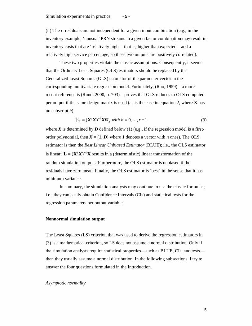
(ii) The r residuals are not independent for a given input combination (e.g., in the

inventory example, ‘unusual' PRN streams in a given factor combination may result in

inventory costs that are ‘relatively high'—that is, higher than expected—and a

relatively high service percentage, so these two outputs are positively correlated).

These two properties violate the classic assumptions. Consequently, it seems

that the Ordinary Least Squares (OLS) estimators should be replaced by the

Generalized Least Squares (GLS) estimator of the parameter vector in the

corresponding multivariate regression model. Fortunately, (Rao, 1959)—a more

recent reference is (Ruud, 2000, p. 703)—proves that GLS reduces to OLS computed

per output if the same design matrix is used (as is the case in equation 2, where X has

no subscript h):

1,,0)’(ˆ 1 −== − rhwithhh �wXXX (3)

where X is determined by D defined below (1) (e.g., if the regression model is a first-

order polynomial, then X = (1, D) where 1 denotes a vector with n ones). The OLS

estimator is then the Best Linear Unbiased Estimator (BLUE); i.e., the OLS estimator

is linear: XXXL 1)’( −= results in a (deterministic) linear transformation of the

random simulation outputs. Furthermore, the OLS estimator is unbiased if the

residuals have zero mean. Finally, the OLS estimator is ‘best’ in the sense that it has

minimum variance.

In summary, the simulation analysts may continue to use the classic formulas;

i.e., they can easily obtain Confidence Intervals (CIs) and statistical tests for the

regression parameters per output variable.

Nonnormal simulation output

The Least Squares (LS) criterion that was used to derive the regression estimators in

(3) is a mathematical criterion, so LS does not assume a normal distribution. Only if

the simulation analysts require statistical properties—such as BLUE, CIs, and tests—

then they usually assume a normal distribution. In the following subsections, I try to

answer the four questions formulated in the Introduction.

Asymptotic normality


6

Simulation responses within a run are autocorrelated (serially correlated). By

definition, a stationary covariance process has a constant mean and a constant

variance; its covariances depend only on the lag |t - t _�EHWZHHQ�WKH�YDULDEOHV� tw and

’tw . The average of a stationary covariance process is asymptotically normally

distributed if the covariances tend to zero sufficiently fast for large lags; see

(Lehmann, 1999, Chapter 2.8). For example, in inventory simulation the output is

often the costs averaged over the simulated periods; I expect this average to be

normally distributed. Another output of an inventory simulation may be the service

percentage calculated as the fraction of demand delivered from on-hand stock per

(say) week, so ‘the' output is the average per year computed from these 52 weekly

averages. I expect this yearly average to be normally distributed—unless the service

goal is ‘close' to 100%, in which case the average service rate is cut off at this

threshold and I expect the normal distribution to be a bad approximation.

Note that CIs based on Student's t statistic are known to be quite insensitive to

nonnormality, whereas the lack-of-fit F-statistic is known to be more sensitive to

nonnormality; see (Kleijnen, 1987) for details including references.

In summary, a limit theorem may explain why simulation outputs are

asymptotically normally distributed. Whether the actual simulation run is long

enough, is always hard to know. Therefore it seems good practice to check whether

the normality assumption holds (see the next subsection).

Testing the normality assumption

Basic statistics textbooks—also see (Arcones and Wang, 2006)—and simulation

textbooks—see (Kleijnen, 1987) and (Law and Kelton, 2000)—propose several visual

plots and goodness-of-fit statistics to test whether a set of observations come from a

specific distribution type such as a normal distribution. A basic assumption is that

these observations are IID. Simulation analysts may therefore obtain ‘many' (say, m =

100) replicates for a specific factor combination (e.g., the base scenario) if

computationally feasible. However, if a single simulation run takes relatively much

computer time, then only ‘a few' (say, 2 ��m ��UHSOLFDWHV�DUH�IHDVLEOH��VR�WKH�SORWV�

are too rough and the goodness-of-fit tests lack power (high probability of type-II

error).


7

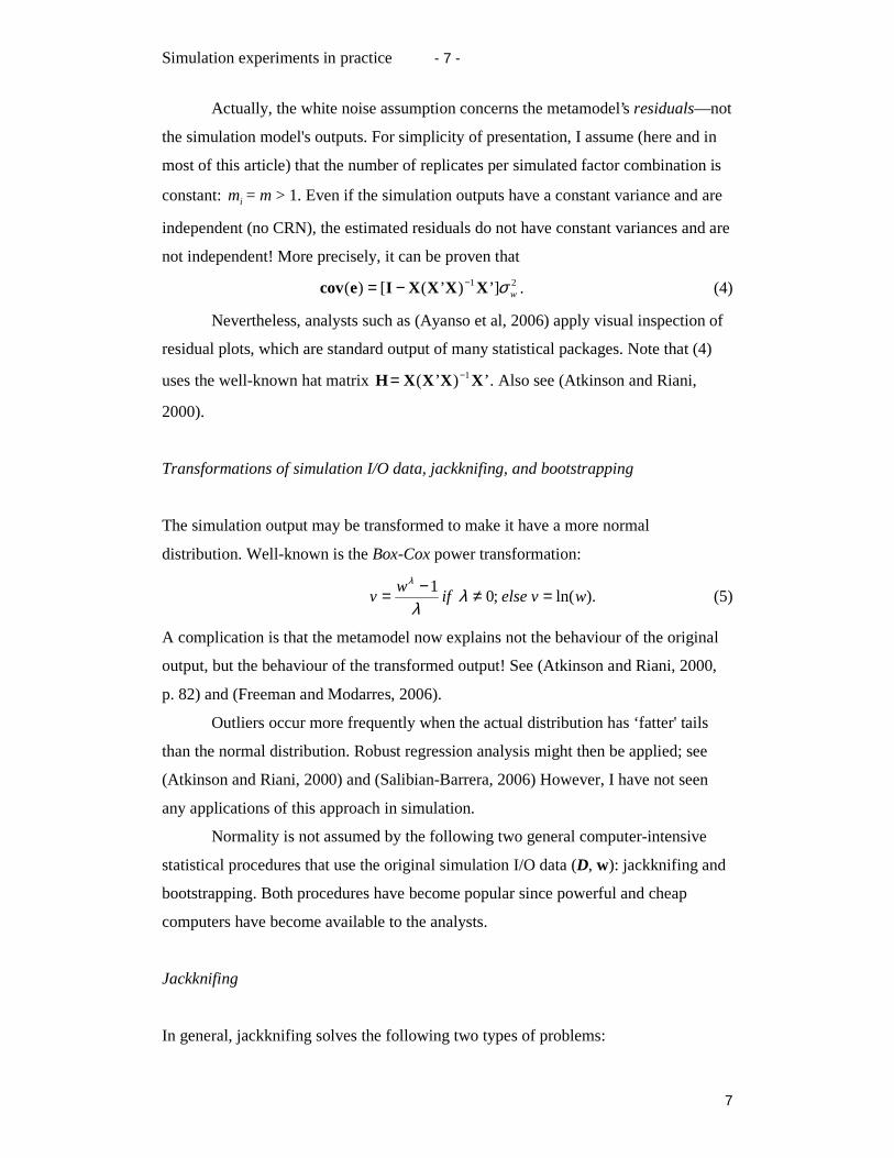
Actually, the white noise assumption concerns the metamodel’s residuals—not

the simulation model's outputs. For simplicity of presentation, I assume (here and in

most of this article) that the number of replicates per simulated factor combination is

constant: im = m > 1. Even if the simulation outputs have a constant variance and are

independent (no CRN), the estimated residuals do not have constant variances and are

not independent! More precisely, it can be proven that

21 ]’)’([)( wσXXXXIecov −−= . (4)

Nevertheless, analysts such as (Ayanso et al, 2006) apply visual inspection of

residual plots, which are standard output of many statistical packages. Note that (4)

uses the well-known hat matrix ’)’( 1 XXXXH −= . Also see (Atkinson and Riani,

2000).

Transformations of simulation I/O data, jackknifing, and bootstrapping

The simulation output may be transformed to make it have a more normal

distribution. Well-known is the Box-Cox power transformation:

).ln(;01

wvelseifw

v =≠−= λλ

λ

(5)

A complication is that the metamodel now explains not the behaviour of the original

output, but the behaviour of the transformed output! See (Atkinson and Riani, 2000,

p. 82) and (Freeman and Modarres, 2006).

Outliers occur more frequently when the actual distribution has ‘fatter' tails

than the normal distribution. Robust regression analysis might then be applied; see

(Atkinson and Riani, 2000) and (Salibian-Barrera, 2006) However, I have not seen

any applications of this approach in simulation.

Normality is not assumed by the following two general computer-intensive

statistical procedures that use the original simulation I/O data (D, w): jackknifing and

bootstrapping. Both procedures have become popular since powerful and cheap

computers have become available to the analysts.

Jackknifing

In general, jackknifing solves the following two types of problems:


8

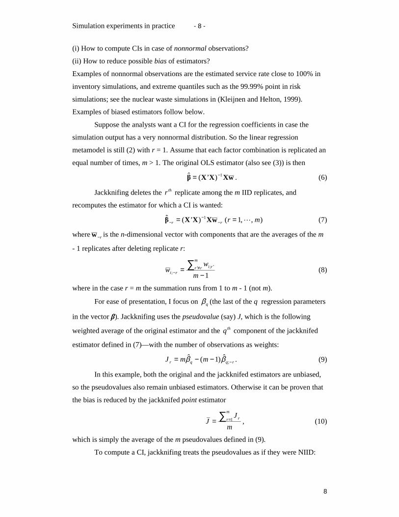
(i) How to compute CIs in case of nonnormal observations?

(ii) How to reduce possible bias of estimators?

Examples of nonnormal observations are the estimated service rate close to 100% in

inventory simulations, and extreme quantiles such as the 99.99% point in risk

simulations; see the nuclear waste simulations in (Kleijnen and Helton, 1999).

Examples of biased estimators follow below.

Suppose the analysts want a CI for the regression coefficients in case the

simulation output has a very nonnormal distribution. So the linear regression

metamodel is still (2) with r = 1. Assume that each factor combination is replicated an

equal number of times, m > 1. The original OLS estimator (also see (3)) is then

wXXX 1)’(ˆ −= . (6)

Jackknifing deletes the thr replicate among the m IID replicates, and

recomputes the estimator for which a CI is wanted:

),,1()’(ˆ 1 mrrr �== −−

− wXXX (7)

where r−w is the n-dimensional vector with components that are the averages of the m

- 1 replicates after deleting replicate r:

1’ ’;

; −= ∑ ≠

− m

ww

m

rr ri

ri (8)

where in the case r = m the summation runs from 1 to m - 1 (not m).

For ease of presentation, I focus on qβ (the last of the q regression parameters

in the vector ). Jackknifing uses the pseudovalue (say) J, which is the following

weighted average of the original estimator and the thq component of the jackknifed

estimator defined in (7)—with the number of observations as weights:

rqqr mmJ −−−= ;ˆ)1(ˆ ββ . (9)

In this example, both the original and the jackknifed estimators are unbiased,

so the pseudovalues also remain unbiased estimators. Otherwise it can be proven that

the bias is reduced by the jackknifed point estimator

m

JJ

m

r r∑ == 1 , (10)

which is simply the average of the m pseudovalues defined in (9).

To compute a CI, jackknifing treats the pseudovalues as if they were NIID:


9

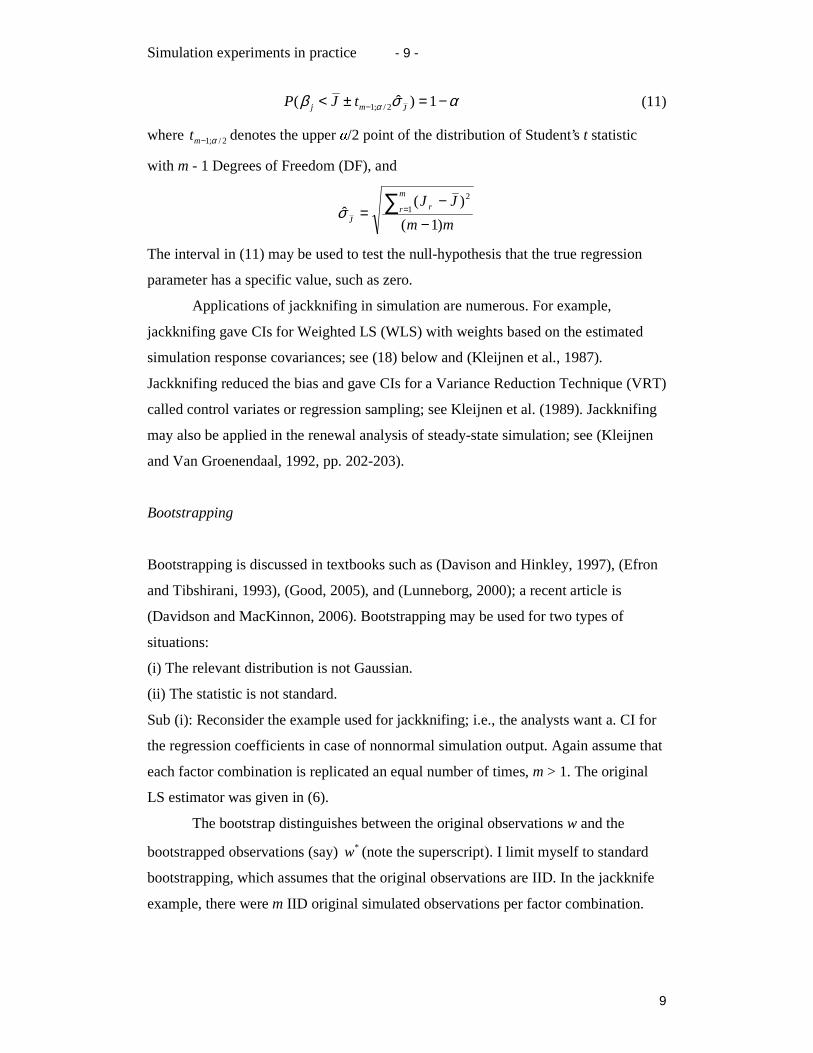
ασβ α −=±< − 1)ˆ( 2/;1 Jmj tJP (11)

where 2/;1 α−mt denotes the upper /2 point of the distribution of Student’s t statistic

with m - 1 Degrees of Freedom (DF), and

mm

JJm

r r

J )1(

)(ˆ 1

2

−−

= ∑ =σ

The interval in (11) may be used to test the null-hypothesis that the true regression

parameter has a specific value, such as zero.

Applications of jackknifing in simulation are numerous. For example,

jackknifing gave CIs for Weighted LS (WLS) with weights based on the estimated

simulation response covariances; see (18) below and (Kleijnen et al., 1987).

Jackknifing reduced the bias and gave CIs for a Variance Reduction Technique (VRT)

called control variates or regression sampling; see Kleijnen et al. (1989). Jackknifing

may also be applied in the renewal analysis of steady-state simulation; see (Kleijnen

and Van Groenendaal, 1992, pp. 202-203).

Bootstrapping

Bootstrapping is discussed in textbooks such as (Davison and Hinkley, 1997), (Efron

and Tibshirani, 1993), (Good, 2005), and (Lunneborg, 2000); a recent article is

(Davidson and MacKinnon, 2006). Bootstrapping may be used for two types of

situations:

(i) The relevant distribution is not Gaussian.

(ii) The statistic is not standard.

Sub (i): Reconsider the example used for jackknifing; i.e., the analysts want a. CI for

the regression coefficients in case of nonnormal simulation output. Again assume that

each factor combination is replicated an equal number of times, m > 1. The original

LS estimator was given in (6).

The bootstrap distinguishes between the original observations w and the

bootstrapped observations (say) *w (note the superscript). I limit myself to standard

bootstrapping, which assumes that the original observations are IID. In the jackknife

example, there were m IID original simulated observations per factor combination.


10

The bootstrap observations are obtained by resampling with replacement from

the original observations, while the sample size is kept constant, at m. This resampling

is executed for each of the n combinations. These bootstrapped outputs give the

bootstrapped average simulation output. Substitution into (6) gives the bootstrapped

LS estimator

*1* )’(ˆ wXXX −= . (12)

To reduce sampling variation, this resampling is repeated (say) B times; B is

known as the bootstrap sample size (typical values for B are 100 and 1,000).

Let’s again focus on the single regression parameter, qβ . The bootstrap literature

gives several CIs, but most popular is the following procedure. Determine the

Empirical Density Function (EDF) of the bootstrap estimate; i.e., sort the B

observations from smallest to largest. The lower limit of the CI is the /2 quantile of

the EDF; i.e., % /2 values are smaller than this quantile. Likewise, the upper limit is

the 1 - /2 quantile.

Applications of bootstrapping include (Kleijnen et al., 2001), which uses

bootstrapping to validate trace-driven simulation models in case of serious nonnormal

outputs.

Sub (ii): Besides classic statistics such as the t and F statistics, the simulation

analysts may be interested in statistics that have no tables with critical values, which

provide CIs—assuming normality. For example, (Kleijnen and Deflandre, 2006)

bootstraps R² to test the validity of regression metamodels in simulation.

Heterogeneous simulation output variances

In the following subsections, I try to answer the five questions raised in the

Introduction.

Common variances in practice?

In practice, the variances of the simulation outputs change when factor combinations

change. For example, in the M/M/1 queuing simulation not only the mean of the

steady-state waiting time changes as the traffic rate changes—the variance of this

output changes even more!


11

Testing the common variance assumption

Though it may be a priori certain that the variances of the simulation outputs are not

constant, the analysts may still hope that the variances are (nearly) constant in their

particular application. Unfortunately, the variances are unknown so they must be

estimated. This estimator itself has high variance. Moreover, there are n factor

combinations in the simulation experiment, so n variance estimators need to be

compared. This problem may be solved in many different ways, but I recommend the

distribution-free test in (Conover, 1980, p. 241).

Variance stabilizing transformations

The logarithmic transformation in (5) may be used not only to obtain normal output

but also to obtain outputs with constant variances. A problem may again be that the

regression metamodel now explains the transformed output instead of the original

output.

Weighted Least Squares (WLS)

In case of heterogeneous variances, the LS criterion still gives an unbiased estimator.

The variance of the LS (or OLS) estimator, however, now is

11 )()cov(’)’()ˆcov( −−= XX’XwXXX . (13)

where the thi (i = 1, …, n) element on the main diagonal of )cov(w is mwi /)var( .

When discussing CRN below, I shall present a simple method to derive CIs for the q

individual OLS estimators; see (24).

Though the OLS estimator remains unbiased, it is no longer the BLUE. It can

be proven that the BLUE is now the WLS estimator

wwXXwcovX 111 )cov(’))(’(~ −−−= NNN . (14)

where I explicitly denote the number of rows N = ∑ =

n

i im1

of X, which is an N×q

matrix. For a constant number of replicates the WLS estimator may be written as

wwcovX’XwcovX 111 )())(’(~ −−−= . (15)


12

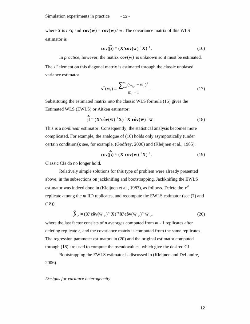
where X is n×q and )(wcov = m/)(wcov . The covariance matrix of this WLS

estimator is

11 ))’()~

cov( −−= Xwcov(X . (16)

In practice, however, the matrix )(wcov is unknown so it must be estimated.

The thi element on this diagonal matrix is estimated through the classic unbiased

variance estimator

1

)()(

2

1 ;2

−−

= ∑ =

i

i

m

r ri

i m

wwws

i

. (17)

Substituting the estimated matrix into the classic WLS formula (15) gives the

Estimated WLS (EWLS) or Aitken estimator:

wwvocXXwvocX 111 )(ˆ'))(ˆ'(~ −−−= . (18)

This is a nonlinear estimator! Consequently, the statistical analysis becomes more

complicated. For example, the analogue of (16) holds only asymptotically (under

certain conditions); see, for example, (Godfrey, 2006) and (Kleijnen et al., 1985):

11 ))('()~

cov( −−≈ XwcovX . (19)

Classic CIs do no longer hold.

Relatively simple solutions for this type of problem were already presented

above, in the subsections on jackknifing and bootstrapping. Jackknifing the EWLS

estimator was indeed done in (Kleijnen et al., 1987), as follows. Delete the thr

replicate among the m IID replicates, and recompute the EWLS estimator (see (7) and

(18)):

rrrr −−

−−−

−− = wwvocXXwv(ocX’ 111 )(ˆ'))ˆ(~

. (20)

where the last factor consists of n averages computed from m - 1 replicates after

deleting replicate r, and the covariance matrix is computed from the same replicates.

The regression parameter estimators in (20) and the original estimator computed

through (18) are used to compute the pseudovalues, which give the desired CI.

Bootstrapping the EWLS estimator is discussed in (Kleijnen and Deflandre,

2006).

Designs for variance heterogeneity


13

If the output variances are not constant, classic designs still give unbiased OLS and

WLS estimators. The literature pays little attention to the derivation of alternative

designs for heterogeneous output variances. (Kleijnen and Van Groenendaaal, 1995)

investigates designs in which factor combinations are replicated so many times that

the estimated variances of the average simulation response per combination are

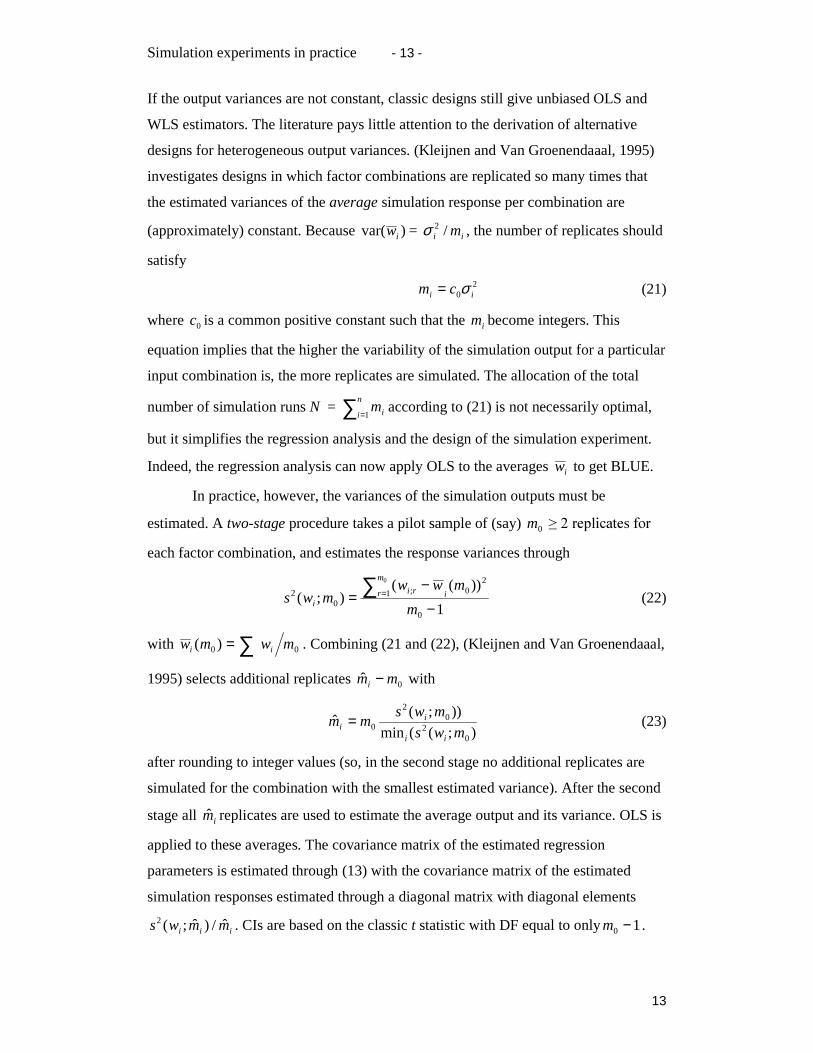
(approximately) constant. Because )var( iw = ii m/2σ , the number of replicates should

satisfy

20 ii cm σ= (21)

where 0c is a common positive constant such that the im become integers. This

equation implies that the higher the variability of the simulation output for a particular

input combination is, the more replicates are simulated. The allocation of the total

number of simulation runs N = ∑ =

n

i im1

according to (21) is not necessarily optimal,

but it simplifies the regression analysis and the design of the simulation experiment.

Indeed, the regression analysis can now apply OLS to the averages iw to get BLUE.

In practice, however, the variances of the simulation outputs must be

estimated. A two-stage procedure takes a pilot sample of (say) 0m ��UHSOLFDWHV�IRU�

each factor combination, and estimates the response variances through

1

))(();(

0

201 ;

02

0

−−

= ∑ =

m

mwwmws i

m

r ri

i (22)

with 00 )( mwmw ii ∑= . Combining (21 and (22), (Kleijnen and Van Groenendaaal,

1995) selects additional replicates 0ˆ mmi − with

);((min

));(ˆ

02

02

0 mws

mwsmm

ii

ii = (23)

after rounding to integer values (so, in the second stage no additional replicates are

simulated for the combination with the smallest estimated variance). After the second

stage all im replicates are used to estimate the average output and its variance. OLS is

applied to these averages. The covariance matrix of the estimated regression

parameters is estimated through (13) with the covariance matrix of the estimated

simulation responses estimated through a diagonal matrix with diagonal elements

iii mmws ˆ/)ˆ;(2 . CIs are based on the classic t statistic with DF equal to only 10 −m .


14

Because these iii mmws ˆ/)ˆ;(2 may still differ considerably, this two-stage approach

may be replaced by a sequential approach. The latter approach adds one replicate at a

time after the pilot stage, until the estimated variances of the average simulation

outputs have become constant; see (Kleijnen and Van Groenendaal, 1995). This

procedure requires fewer simulation responses than the two-stage procedure, but is

harder to understand, program, and implement.

Common Random Numbers (CRN)

In the following subsections, I try to answer the questions raised in the Introduction.

CRN use in practice

In practice, simulation analysts often use CRN. Actually, CRN is the default of much

simulation software; i.e., the software automatically starts each run with the same

PRN seed. For example, let’s consider an M/D/1 simulation (exponential interarrival

times, constant service times, single server). For illustration purposes, consider a very

extreme (unlikely) event, namely all the PRNs happen to be close to one. Then the

interarrival times are close to zero. So, whatever traffic rate is simulated, the waiting

times tend to be higher than expected; i.e., the simulation responses of the different

traffic rates are positively correlated.

In general, CRN implies that the simulation outputs of different factor

combinations are correlated across these combinations. The goal is to reduce the

variances of the estimated factor effects; actually, the variance of the estimated

intercept increases when CRN are used. CRN gives better predictions of the output for

combinations not yet simulated—provided the inaccuracy of the estimated intercept is

outweighed by the accuracy of all other estimated effects.

OLS versus Estimated Generalized Least Squares

Because CRN violates the a classic assumption of regression analysis (namely, the

simulation outputs are independent, not correlated), the analysts have two options:

(i) Continue to use OLS


15

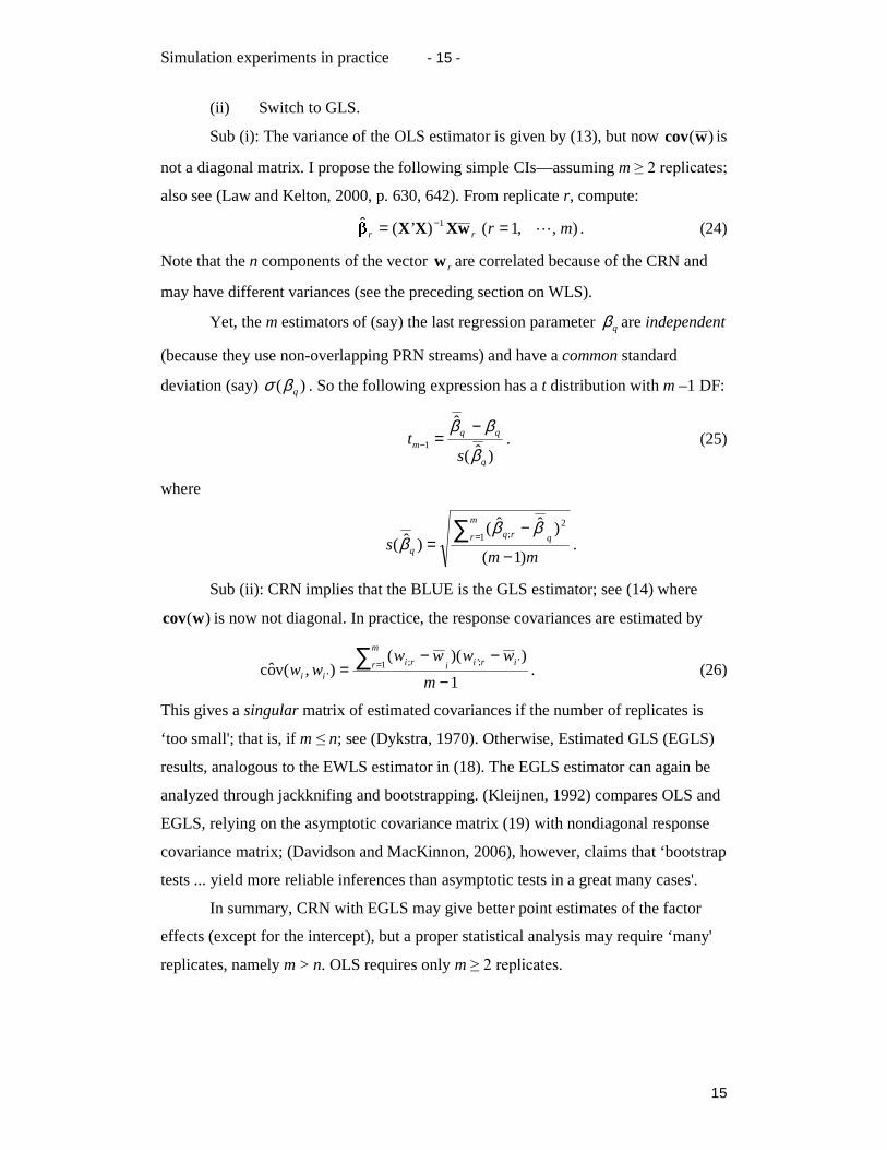
(ii) Switch to GLS.

Sub (i): The variance of the OLS estimator is given by (13), but now )(wcov is

not a diagonal matrix. I propose the following simple CIs—assuming m ��UHSOLFDWHV��

also see (Law and Kelton, 2000, p. 630, 642). From replicate r, compute:

),,1()’(ˆ 1 mrrr �== − wXXX . (24)

Note that the n components of the vector rw are correlated because of the CRN and

may have different variances (see the preceding section on WLS).

Yet, the m estimators of (say) the last regression parameter qβ are independent

(because they use non-overlapping PRN streams) and have a common standard

deviation (say) )( qβσ . So the following expression has a t distribution with m –1 DF:

)ˆ(

ˆ1

q

qqm

st

β

ββ −=− . (25)

where

mms q

m

r rq

q )1(

)ˆˆ()ˆ(

2

1 ;

−

−=

∑ =ββ

β .

Sub (ii): CRN implies that the BLUE is the GLS estimator; see (14) where

)(wcov is now not diagonal. In practice, the response covariances are estimated by

1

))((),v(oc

’;’1 ;

’ −

−−= ∑ =

m

wwwwww

irii

m

r ri

ii . (26)

This gives a singular matrix of estimated covariances if the number of replicates is

‘too small'; that is, if m ��n; see (Dykstra, 1970). Otherwise, Estimated GLS (EGLS)

results, analogous to the EWLS estimator in (18). The EGLS estimator can again be

analyzed through jackknifing and bootstrapping. (Kleijnen, 1992) compares OLS and

EGLS, relying on the asymptotic covariance matrix (19) with nondiagonal response

covariance matrix; (Davidson and MacKinnon, 2006), however, claims that ‘bootstrap

tests ... yield more reliable inferences than asymptotic tests in a great many cases'.

In summary, CRN with EGLS may give better point estimates of the factor

effects (except for the intercept), but a proper statistical analysis may require ‘many'

replicates, namely m > n. OLS requires only m ��UHSOLFDWHV�


16

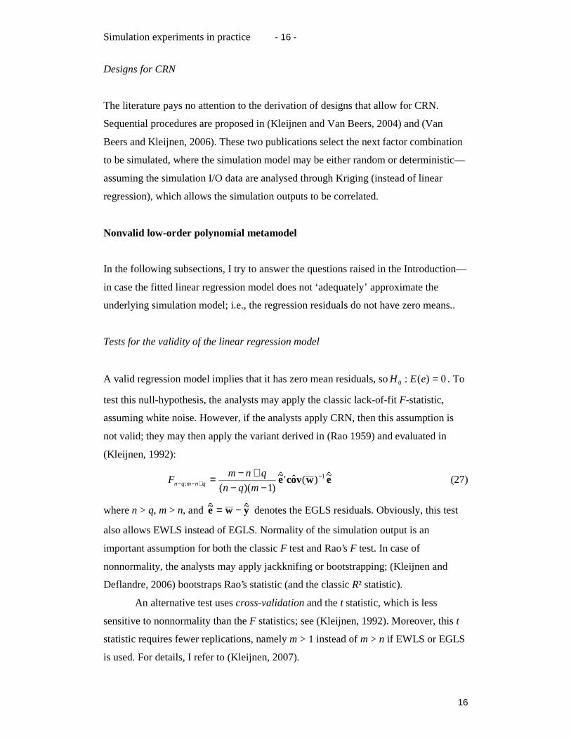
Designs for CRN

The literature pays no attention to the derivation of designs that allow for CRN.

Sequential procedures are proposed in (Kleijnen and Van Beers, 2004) and (Van

Beers and Kleijnen, 2006). These two publications select the next factor combination

to be simulated, where the simulation model may be either random or deterministic—

assuming the simulation I/O data are analysed through Kriging (instead of linear

regression), which allows the simulation outputs to be correlated.

Nonvalid low-order polynomial metamodel

In the following subsections, I try to answer the questions raised in the Introduction—

in case the fitted linear regression model does not ‘adequately’ approximate the

underlying simulation model; i.e., the regression residuals do not have zero means..

Tests for the validity of the linear regression model

A valid regression model implies that it has zero mean residuals, so 0)(:0 =eEH . To

test this null-hypothesis, the analysts may apply the classic lack-of-fit F-statistic,

assuming white noise. However, if the analysts apply CRN, then this assumption is

not valid; they may then apply the variant derived in (Rao 1959) and evaluated in

(Kleijnen, 1992):

ewvoce ~)(ˆ'~)1)((

1;

−+−− −−

+−=mqn

qnmF qnmqn (27)

where n > q, m > n, and ywe ~~ −= denotes the EGLS residuals. Obviously, this test

also allows EWLS instead of EGLS. Normality of the simulation output is an

important assumption for both the classic F test and Rao’s F test. In case of

nonnormality, the analysts may apply jackknifing or bootstrapping; (Kleijnen and

Deflandre, 2006) bootstraps Rao’s statistic (and the classic R² statistic).

An alternative test uses cross-validation and the t statistic, which is less

sensitive to nonnormality than the F statistics; see (Kleijnen, 1992). Moreover, this t

statistic requires fewer replications, namely m > 1 instead of m > n if EWLS or EGLS

is used. For details, I refer to (Kleijnen, 2007).


17

Besides these quantitative tests, the analysts may use graphical methods to

judge the validity of a fitted metamodel (be it a linear regression model or some other

type of metamodel such as a Kriging model). Scatterplots are well known. The panel

discussion published in (Simpson et al., 2004) also emphasizes the importance of

visualization; also see (Helton et al., 2006). If these validation tests reject the null-

hypothesis, then the analysts may consider the alternatives discussed in the next

subsection.

Transformations for improved validity of regression model

A well-known transformation in queuing simulations combines two simulation

inputs—namely, the arrival rate (say) �DQG�WKH�VHUYLFH�UDWH� —into a single

independent regression variable—QDPHO\��WKH�WUDIILF�UDWH� � ��$QRWKHU�WUDQVIRUPDWLRQ�

UHSODFHV�\�� DQG� �E\�ORJ�\��ORJ� ��DQG�ORJ� ��WR�PDNH�WKH�ILUVW-order polynomial

approximate relative changes.

Still another simple transformation assumes that the I/O function of the

underlying simulation model is monotonic. Then the dependent and independent

variables may be replaced by their ranks, which results in so-called rank regression;

see (Conover and Iman, 1981) and (Saltelli and Sobol, 1995). (Kleijnen and Helton,

1999) applies rank regression to find the most important factors in a simulation model

of nuclear waste disposal.

Transformations may also be applied to make the simulation output

(dependent regression variable) better satisfy the assumptions of normality (see (5))

and variance homogeneity. Unfortunately, different goals of the transformation may

conflict with each other; for example, the analysts may apply the logarithmic

transformation to reduce nonnormality, but this transformation may give a metamodel

in variables that are not of immediate interest.

I do not recommend routinely augment the metamodel with higher-order

terms (e.g., interactions among triplets of factors) because these terms are hard to

interpret. However, if the analysts’ goal is not to understand the underlying

simulation model but to predict the output of an expensive simulation model, then

high-order terms may be added. Indeed, classic full-factorial designs enable the

estimation of all interactions (not only the many two-factor interactions, but also the


18

single interaction among all k factors). If more than two levels are simulated per

factor, then the following types of metamodels may be considered.

Alternative metamodels

There are several alternative metamodel types; for example, Kriging and neural

network models. These alternatives may give better predictions than low-order

polynomials do. However, these alternatives are so complicated that they do not help

the analysts better understand the underlying simulation model. Furthermore, these

alternative metamodels require alternative design types. This is a completely different

issue, so I refer to the extensive literature on this topic—including (Kleijnen, 2007).

Conclusions

In this survey, I discussed the assumptions of classic linear regression analysis and the

concomitant statistical designs. I pointed out that multivariate simulation output may

still be analysed through OLS. I addressed possible nonnormality of simulation

output, including normality tests, transformations of simulation I/O data, jackknifing,

and bootstrapping. I presented analysis and design methods for heteroscedastic

simulation output. I discussed how to analyse simulation outputs that use CRN. I

discussed possible lack-of-fit of low-order polynomial metamodels, and possible

remedies. I gave many references for further study of these issues.

I hope that practitioners will be stimulated to apply this statistical

methodology to obtain more information from their simulation experiments.

Statistical designs can be proven to be much better than designs changing only one

factor at a time. Regression models formalize scatter plots and other popular graphical

techniques for analysing the simulation model’s I/O data.

Finally, I hope that this methodology will be incorporated in future simulation

software.

References


19

Angün E, den Hertog D, Gürkan G and Kleijnen J P C (2006), Response surface

methodology with stochastic constrains for expensive simulation. Working Paper,

Tilburg University, Tilburg, Netherlands.

Arcones M.A. and Wang Y (2006), Some new tests for normality based on U-

processes. Statistics & Probability Letters, 76: 69-82.

Atkinson, A and Riani M (2000), Robust diagnostic regression analysis. Springer:

New York.

Ayanso A, Diaby M and Nair S K(2006), Inventory rationing via drop-shipping in

Internet retailing: a sensitivity analysis. European Journal of Operational Research,

171: 135-152.

Conover W.J. (1980), Practical nonparametric statistics: second edition. Wiley: New

York.

Conover W.J. and Iman R L (1981), Rank transformations as a bridge between

parametric and nonparametric statistics. The American Statistician, 35: 124-133.

Davidson R. and MacKinnon J G (2006), Improving the reliability of bootstrap tests

with the fast double bootstrap Computational Statistics & Data Analysis, in press

Davison A.C. and Hinkley D V (1997), Bootstrap methods and their application.

Cambridge University Press: Cambridge.

Dykstra R L (1970), Establishing the positive definiteness of the sample covariance

matrix. The Annals of Mathematical Statistics, 41: 2153-2154.

Efron, B and Tibshirani R J (1993), An introduction to the bootstrap. Chapman &

Hall: New York.

Freeman, J and Modarres R (2006), Inverse Box Cox: the power-normal distribution

Statistics & Probability Letters, 76: 764-772.

Godfrey L G (2006), Tests for regression models with heteroskedasticity of unknown

form Computational Statistics & Data Analysis, 50, no. 10: 2715-2733.

Good P I (2005), Resampling methods: a practical guide to data analysis; third

edition. Birkhäuser: Boston.

Helton, J C , Johnson J D, Sallaberry C J and Storlie C B (2006), Survey of

sampling-based methods for uncertainty and sensitivity analysis. Reliability

Engineering and Systems Safety, in press.

Ivanescu C, Bertrand W, Fransoo J and Kleijnen J P C (2006), Bootstrapping to solve

the limited data problem in production control: an application in batch processing

industries. J Opl Res Soc 57: 2-9.


20

Kleijnen J P C (1987), Statistical tools for simulation practitioners. Marcel Dekker:

New York.

Kleijnen J P C (1992), Regression metamodels for simulation with common random

numbers: comparison of validation tests and confidence intervals. Management

Science, 38: 1164-1185.

Kleijnen J P C (1993), Simulation and optimization in production planning: a case

study. Decision Support Systems, 9: 269-280.

Kleijnen J P C (2006), White noise assumptions revisited: Regression metamodels

and experimental designs for simulation practice. Proceedings of the 2006 Winter

Simulation Conference, edited by L. F. Perrone, F. P. Wieland, J. Liu, B. G. Lawson,

D. M. Nicol and R. M. Fujimoto: 107-117.

Kleijnen J P C (2007), DASE: Design and analysis of simulation experiments.

Springer Science + Business Media.

Kleijnen J P C, Cheng R C H and Bettonvil B (2001), Validation of trace-driven

simulation models: bootstrapped tests. Management Science, 47, no. 11: 1533-1538.

Kleijnen J P C, Cremers P and Van Belle F (1985), The power of weighted and

ordinary least squares with estimated unequal variances in experimental designs.

Communications in Statistics, Simulation and Computation, 14, no. 1: 85-102.

Kleijnen J P C and Deflandre D (2006), Validation of regression metamodels in

simulation: Bootstrap approach. European Journal of Operational Research, 170: 120-

131.

Kleijnen J P C and Helton J C (1999), Statistical analyses of scatter plots to identify

important factors in large-scale simulations, 1: review and comparison of techniques.

Reliability Engineering and Systems Safety, 65: 147-185.

Kleijnen J P C, Karremans P C A , Oortwijn W K and Van Groenendaal W J H

(1987), Jackknifing estimated weighted least squares: JEWLS. Communications in

Statistics, Theory and Methods, 16: 747-764.

Kleijnen J P C , Kriens J , Timmermans H and Van den Wildenberg H (1989),

Regression sampling in statistical auditing: a practical survey and evaluation

(including Rejoinder). Statistica Neerlandica, 43: 193-207, 225.

Kleijnen J P C and Van Beers W C M (2004), Application-driven sequential designs

for simulation experiments: Kriging metamodeling. J Opl Res Soc, 55: 876-883.

Kleijnen J P C and Van Groenendaal W J H (1992), Simulation: a statistical

perspective. John Wiley: Chichester.


21

Kleijnen J P C and Van Groenendaal W J H (1995), Two-stage versus sequential

sample-size determination in regression analysis of simulation experiments. American

Journal of Mathematical and Management Sciences, 15: 83-114.

Law A M and Kelton W D (2000), Simulation modeling and analysis; third edition.

McGraw-Hill: Boston.

Lehmann E L (1999), Elements of large-sample theory, Springer, New York

Lunneborg C E (2000), Data analysis by resampling: concepts and applications.

Duxbury Press: Pacific Grove, California.

Rao C R (1959), Some problems involving linear hypothesis in multivariate analysis.

Biometrika, 46: 49-58.

Rao C R (1967), Least squares theory using an estimated dispersion matrix and its

application to measurement of signals. Proceedings of the Fifth Berkeley Symposium

on Mathematical Statistics and Probability, I: 355-372.

Ruud P A (2000), An introduction to classical econometric theory. Oxford University

Press: New York.

Salibian-Barrera M (2006), Bootstrapping MM-estimators for linear regression with

fixed designs. Statistics & Probability Letters, in press.

Saltelli A and Sobol I M (1995), About the use of rank transformation in sensitivity

analysis of model output. Reliability Engineering and System Safety, 50: 225-239.

Simpson T W, Booker A J, Ghosh D, Giunta A A, Koch, P N and Yang, R (2004),

Approximation methods in multidisciplinary analysis and optimization: a Panel

discussion. Structural and Multidisciplinary Optimization, 27, no. 5: 302-313.

Van Beers W C M and Kleijnen J P C (2006), Customized sequential designs for

random simulation experiments: Kriging metamodeling and bootstrapping. Working

Paper, Tilburg University, Tilburg, Netherlands.

no. 2007–09 simulation experiments in practice

Documents