atlantos observing system simulation experiments (osses
TRANSCRIPT
Last updated: 10 October 2018
This project has received funding from the European Union’s Horizon 2020 research and
innovation programme under grant agreement no 633211.
Project AtlantOS – 633211
Deliverable number 1.5
Deliverable title Synthesis of OSSE results
Description Observing System Simulation Experiments (OSSEs): Report describing the robust results obtained from across the models.
Work Package number 1
Work Package title Observing System Requirements and Design Studies
Lead beneficiary Met Office
Lead authors Richard Wood (editor), David Ford, Florent Gasprin, Matthew Palmer, Elisabeth Rémy, Pierre Yves le Traon
Contributors Adam Blaker, Jean-Michel Brankart, Pierre Brasseur, Freya Garry, Marion Gehlen, Cyril Germinaud, Rohit Ghosh, Stéphanie Guinehut, Johann Jungclaus, Robert King, Katja Lohmann, Chongyuan Mao, Matthew Martin, Simona Masina, Vrac Mathieu, Michael Mayer, Isabelle Mirouze, Adrian New, Anna Sommer, Hao Zuo
Submission data
Due date August 2018
Comments An extension to the original deadline was requested to allow time for integration of the results from the complex OSSE intercomparison. This is the first time such an intercomparison has been undertaken.

Synthesis of OSSE results
2
Stakeholder engagement relating to this task*
WHO are your most important stakeholders?
☐ National governmental body
☐ International organization
Please give the name(s) of the stakeholder(s): World Climate Research Programme Global Ocean Observing System
WHERE is/are the company(ies) or organization(s) from?
Please name the country(ies): International
Is this deliverable a success story? If yes, why?
If not, why?
☐ Yes, because the most coordinated set of studies to date has been successfully completed to examine the potential of different options for the future ocean observing system. Specific impacts of different observing elements have been assessed for data assimilating ocean models (analyses), and the need to future-proof the observing system to detect future climate change has been demonstrated and quantified.
Will this deliverable be used?
If yes, who will use it?
If not, why will it not be used?
☐ Yes, the results (and resulting publications in the peer-reviewed literature) will be influential in international thinking about the shape of the future global ocean observing system. For example, the results are expected to be an important input to the once-per-decade OceanObs 2019 conference.
NOTE: This information is being collected for the following purposes: 1. To make a list of all companies/organizations with which AtlantOS partners have had contact.
This is important to demonstrate the extent of industry and public-sector collaboration in the observation community. Please note that we will only publish one aggregated list of companies and not mention specific partnerships.
2. To better report success stories from the AtlantOS community on how observing delivers concrete value to society.
*For ideas about relations with stakeholders you are invited to consult D10.5 Best Practices in Stakeholder Engagement, Data Dissemination and Exploitation.
This project has received funding from the European Union’s Horizon 2020 research and
innovation programme under grant agreement no 633211.
Synthesis of OSSE results
3
Synthesis of OSSE Results Executive Summary Any sustained observing system for the Atlantic Ocean will inevitably be limited in its coverage of the ocean in space and time. To design a cost-efficient observing system requires information on alternative observing and sampling strategies: where should we put our observing resources to maximise the resulting knowledge of the state of the ocean?, and what is the added value of new technologies or networks? To address these questions Task 1.3 of AtlantOS has undertaken a range of model-based studies (‘Observing System Simulation Experiments’ or OSSEs), in which a state-of-the-art ocean or climate model is used to provide a complete (in space and time) ocean state which is taken as a simulated ‘truth’. This ‘truth’ state is sampled using different candidate observing networks, including both historical and possible future networks, and these ‘pseudo-observations’ are used to attempt to reconstruct the original ‘truth state’. The fidelity with which the reconstruction matches the known truth state gives an indication of the effectiveness of the chosen observing strategy. In AtlantOS Task 1.3 we have used a variety of OSSE techniques to assess the effectiveness of recent, current and potential future observing networks. The techniques fall roughly into two classes:
• Data Assimilation OSSEs. In these methods the simulated observations are assimilated into an ocean model (the ‘test model’) using the same or similar methods as are used for current operational oceanography to produce near real time ocean state estimates and forecasts. Model bias is accounted for by using a different model as the test model than was used to produce the ‘truth’ state. Without data assimilation the test model will produce a different ocean state to the ‘truth model’, and the success of the process is evaluated by measuring whether assimilating the pseudo-observations brings the ‘test model’ state closer to the ‘truth’ state. This type of OSSE study is typically used to evaluate the value of candidate observing strategies for operational oceanography. Typical measures of success would be to what extent assimilating a proposed observing network reduces the bias and root-mean-square error in the ‘test model’, when compared to the ‘truth model’. In AtlantOS Task 1.3 we have performed a coordinated set of OSSEs (across four partners) to evaluate the impact of different observations of the physical state of the ocean (Section 2), and a pair of studies (two partners) to assess in different ways the impact of a range of biogeochemical observations (Section 3). The physical study is the first time that such a closely co-ordinated multi-system OSSE study has been completed.
• Climate OSSEs. This is a less developed scientific field and we have performed a variety of research studies across three partners, with a common focus on understanding how well past and future observations can constrain Ocean Heat Content (OHC), a key indicator of global and regional climate change (Section 4). Climate model simulations of the 20th Century and projections for the 21st Century are used to provide a ‘past and future truth’, which is sampled using different observing strategies. As heating from anthropogenic climate change penetrates deeper into the ocean over the 21st Century it is possible that we will need to extend the current observing network deeper if we wish to track the energy budget of the Earth, and we have assessed the needs to ‘future-proof’ the observing network in this way.
Synthesis of OSSE results
4
Detailed discussion of results can be found in sections 2-4 below, with still further detail in a number of individual reports that will be made available through the AtlantOS web site, and in peer-reviewed scientific papers that are currently in preparation. Highlight results include: Physical OSSEs:
1. For the first time, a highly co-ordinated multi-model OSSE has been carried out to assess the potential of a range of observing elements to better estimate the physical state of the Atlantic Ocean. This represents a major advance in the robust evaluation of observing systems.
2. Compared with a baseline physical Argo network which is uniformly distributed across the ocean, increased Argo density in western boundary currents and along the equator results in improved estimates of temperature and salinity for the entire Atlantic. The improvements are particularly noticeable in the 300-2000m depth range.
3. A hypothetical addition of a drifter array to 150m depth results in a significant improvement to the representation of the near-surface layers (complementary to (1) above).
4. A deep Argo array, with 5°x5°spacing and monthly sampling to either 4000m or the bottom,
would lead to substantial improvement in deep temperature and salinity estimates (20-40% error reduction in three out of the four test model systems studied).
5. The present tropical mooring array provides invaluable data for evaluation of models and assimilation systems, and provides atmospheric as well as oceanographic data. Assimilation of the ocean data into current ocean model systems has an impact primarily in the region of the moorings.
6. A complementary study was performed in which a system assimilating real observations from 1993-2015 was taken as the baseline, and different observing elements were then removed to assess their impact. This shows strong degradation of estimated sea surface temperature and top 300m heat content when XBT/Argo profiles are removed, with the degradation strongest in the Atlantic basin.
7. The impact of removing profile data on the resulting seasonal forecasts will be explored elsewhere in AtlantOS (Task 7.4); preliminary statistical studies reported here suggest that there will be a detectable impact on seasonal forecasts of atmospheric variables, but that the detail of this impact is dependent on model resolution.
Biogeochemical OSSEs:
1. Assimilation of satellite ocean colour data is effective for constraining surface
phytoplankton, but adds limited information on other biogeochemical fields at the surface or below.
2. Assimilation of biogeochemical Argo (BGC-Argo) data complements surface colour data by improving model estimates of oxygen, nutrients, carbon and chlorophyll throughout the water column. It also improves surface chlorophyll estimates when satellite colour data are restricted by cloud. Inclusion of BGC sensors on roughly one quarter of the current Argo array (around 1000 floats) provides clear improvements; there is some evidence that a higher density of BGC floats would add further value, but it may be that development of
Synthesis of OSSE results
5
improved data assimilation methods (Bullet 3) could provide similar added value by better exploiting the low density BGC array.
3. Assimilation of in-situ biogeochemical data is relatively immature, and it is expected that further improvements to ocean state estimates could be achieved through development of more advanced assimilation schemes. Work on such developments is currently in progress under Copernicus and various national programmes. Specific issues for development include optimal assimilation of multiple data types, and assimilation methods specifically designed for use with sparse observation networks (bearing in mind the likely sparse nature of BGC-Argo coverage, see Bullet 2.
4. An independent study was performed with a specific focus on the ocean carbon system (surface pCO2). In this case, statistical methods were used to reconstruct the ‘truth’ field from a variety of potential observing networks. It was found that the existing ship-of-opportunity network (SOCAT), enhanced by BGC-Argo sampling in the South Atlantic at around one quarter of current physical Argo resolution, provided an attractive option to obtain a good estimate of the pCO2 field. Further improvements could be obtained from moorings or Argo coverage in the Labrador Sea, Baffin Bay, Norwegian Sea and African coastal regions between 10°N and 20°S.
Climate Perspective:
1. The historical observing network over recent decades was insufficient to fully constrain changes in global OHC from 1960 up to the start of the Argo period1. Different methods of filling the gaps in the observations produce different estimates of past OHC change. However the advent of Argo in the early 2000s led to a significant improvement in OHC estimates, both globally (a measure of global climate change) and regionally (important for forecasting major modes of climate variability).
2. Sampling below the current 2000m depth of Argo (e.g. through Deep Argo floats) is likely to
be important to track OHC and climate change as warming progresses in the 21st Century. This deeper penetration of heat begins to become significant around the year 2000 in the models studied, and is particularly strong in the Atlantic and Southern Oceans, indicating where we may expect to get the greatest added value from early deployment of deep observations.
3. It may be possible to derive greater value from sparse deep observations by spreading the information along constant-density surfaces rather than constant-depth surfaces. Individual observations in the Eastern Atlantic basin appear to be representative of a wider area than individual observations in the West Atlantic, suggesting that higher observing density may be appropriate in the Western basin. In general, salinity observations appear to be representative of a wider area than temperature observations.
4. Observations of ocean heat transport across key latitudes complement observations of OHC, allowing us to understand in greater detail the role of the Atlantic Ocean in climate variability and change. Model studies suggest that monitoring heat transport at both a subtropical (e.g. 26°N RAPID) and a subpolar latitude would be necessary to fully quantify the effect of climate change on the North Atlantic Ocean.
1 We take the target as being able to estimate ocean heat content to within an error of 0.1 Wm-2 in the top-of-atmosphere heat budget of the climate system.

Synthesis of OSSE results
6
While the above results are derived from a limited range of model studies, and further studies would undoubtedly be desirable to add robustness to the conclusions, the results are beginning to give some clear pointers to the added value of particular observing systems. This information can be used to inform future design of both the observing system and the downstream modelling systems that exploit and interpret the observations to provide services and scientific knowledge to society.
Synthesis of OSSE results
7
1. Introduction
Over the three past decades, the development of space-based and in-situ technologies has
significantly increased the number of surface and sub-surface ocean observations. However, while
satellite observations have a nearly global coverage, and are coordinated by national and
international space-agencies, the organization of the in-situ networks is more complex, and often
results from mono-disciplinary actions. In this context, the H2020 AtlantOS project brings together
scientists, stakeholders and industry from around the Atlantic to provide a multinational framework
for more and better-coordinated efforts in observing, understanding and predicting the Atlantic
Ocean (Visbeck et al., 2015). To support the on-going effort undertaken by the oceanographic
community, an internationally coordinated initiative within the AtlantOS project has been conducted
by the European forecasting centers to provide quantitative information of potential impacts of
further evolution of the in-situ networks on global ocean monitoring and forecasting systems.
The present work is based on numerical experiments, called Observing System Simulation
Experiment (OSSE). OSSEs consist in subsampling a “realistic” simulation at the space and time
location of each observation from a given observing system design, and then assimilating it into a
data assimilation system.
It is noteworthy that monitoring and forecasting systems are regarded as one of the key tools to
explore the integration of the Global Ocean Observing System (GOOS), synthesising data from in-
situ platforms and satellites. OSSEs are therefore usually performed in order to support the
evolution of an integrative global ocean observing system, but they also can help to refine data
assimilation schemes in ocean reanalyses and monitoring systems, and to prepare operational
systems to ingest new observations. Several coordinated initiatives are currently handled in the
framework of Global Ocean Data Assimilation Experiment (GODAE) Ocean View (Bell et al., 2015)
such as inter-comparison and validation approaches of the forecasting systems (e.g., Ryan et al.,
2015) and reanalyses (e.g., Balmaseda et al., 2015).
In AtlantOS, we have conducted a coordinated OSSE experiment across several model/data
assimilation systems, to assess the impact of a number of plausible developments to the ocean
observing system for physical variables (Section 2). To our knowledge, this is the first time that
such an internationally coordinated effort is made using OSSE, because these numerical
experiments require heavy and dedicated infrastructures. This multi-model and multi-approach
enables one to discuss the robustness of the results, knowing that OSSE can be strongly model-
dependent (Halliwell, et al., 2014).
Forecasts and reanalyses of ocean biogeochemistry are required for a number of societal,
scientific, and policy applications. An estimated 12% of the global population rely on fisheries and
aquaculture for their livelihoods (FAO, 2016), and fish stocks are dependent on primary
productivity. Water quality and the health and diversity of the marine environment are of paramount
importance, and are regulated by European Union directives such as the Marine Strategy
Framework Directive (MSFD). Climate variability and change, and their associated impacts, must
be monitored and understood, and the North Atlantic, in particular, is an important but variable
carbon sink. Ocean acidification and hypoxia also pose an increasing threat to marine ecosystems.
The observing and forecasting systems for ocean biogeochemistry are not as mature as for the
physical variables, but are developing apace. Remotely sensed ocean colour has provided routine
global observations of optical properties and chlorophyll concentration for over two decades
(McClain, 2009). This has proved an invaluable tool for reanalysis and forecasting (Gehlen et al.,
Synthesis of OSSE results
8
2015), but its coverage is restricted to the near-surface and cloud-free conditions, and limited
information can be obtained about other variables such as nutrient concentrations.
The in-situ observing system consists of various ships, gliders, moorings, and time series stations.
These are of fundamental importance for scientific understanding, and model calibration and
validation. However, observations are sparse and rarely available in near-real-time, so often have
limited value for operational applications.
We have performed observing system simulation experiments (OSSEs) to assess the impact on
the models of assimilating different potential biogeochemical observing arrays based on the
relatively new biogeochemical Argo floats (BGC-Argo). These experiments assess the value that
assimilating BGC-Argo data would add to the existing satellite ocean colour system. Two different
methodologies have been developed and compared, by CNRS/IGE and the Met Office. Each
focuses on the potential of biogeochemical Argo floats to improve knowledge of the
biogeochemical state of the ocean (Section 3).
A collection of studies has been carried out to assess the priorities for the current and future ocean
observing system in the context of climate detection, monitoring and prediction (Section 4). This
work adopts a range of approaches that goes beyond standard data assimilation systems. It
focuses primarily on ocean temperature change, both in terms of ocean heat content change
(OHC), and also the northward heat transport in the North Atlantic, which is a key factor in the
relatively mild climate of Western Europe. Global OHC change is our primary means of estimating
the magnitude of Earth’s energy imbalance, and therefore a key metric for monitoring
anthropogenic climate change. Variability in OHC can give rise to predictability of the ocean and
climate on seasonal-to-decadal timescales. As anthropogenic climate warming penetrates into the
ocean, it may be that deeper observations are required to continue to keep track of the Earth’s
energy budget. We assess the need for such ‘future-proofing’ of the observing system.
Synthesis of OSSE results
9
2. Physical OSSEs
This study uses four global eddy-permitting systems, i.e. three analysis and forecasting systems
and one model-independent analysis system. This work results from exchanges and discussions
with in-situ networks, and focuses on the evolution of Argo floats (Roemmich et al., 2009), drifting
buoys (Lumpkin et al., 2007) and fixed-mooring (McPhaden et al., 2010) arrays. The report is
organized as follows. Section 2.1 briefly presents the OSSE methodology. Section 2.2 presents the
results about the impacts of doubling Argo in WBC and along the equator and extending Argo
below 2000m, plus extending the drifter arrays to 150m depth. Conclusions and discussion of the
OSSE experiments are provided in Section 2.3. Finally in Section 2.4 we present results from a
complementary study (Observing System Experiment or OSE) in which a system assimilating real
historical observations is taken as the baseline and different observation types are removed to
assess their impact on the solution.
2.1 OSSE Methodology
Firstly developed for the atmosphere, the OSSE methodology has a rigorous framework of strategy and validation techniques for ocean OSSEs, as described by Halliwell et al. (2014). The present work follows the specific OSSE requirements exposed in this later paper. Basically, an ocean OSSE system is composed of (i) an unconstrained ocean model to perform the nature run (NR), (ii) a data assimilation system (DAS), i.e., a different ocean model, or a different configuration of the same ocean model, plus data assimilation techniques, and (iii) a software for subsampling the NR and generating synthetic observations.
2.1.1 The Nature Run configuration
The Nature Run corresponds to the single (‘twin-free’) simulation (with no assimilation) of the Mercator Ocean monitoring and forecasting system PSY4V3R1, operated in near-real time by the Copernicus Marine Environment Monitoring Service (CMEMS) since 19 October 2016. This high-resolution global ocean simulation, considered for the purpose of our study as the “true” ocean, is based on version 3.1 of the NEMO ocean model (Madec et al., 2008), which uses a 1/12° ORCA grid type (with a horizontal resolution of 9 km at the equator, 7 km at mid-latitudes and 2 km near the poles). The atmospheric fields, which force the ocean model, are obtained from the European Centre for Medium-Range Weather Forecasts-Integrated Forecast System (ECMWF-IFS) at 3-hr resolution. The PSY4 system was initialized on 11 October 2006, from the EN4 monthly gridded fields of temperature and salinity (Good et al., 2013), averaged for the period October-December 2006. Assuming that the velocity field is zero at the start, the model physics then spins up a velocity field in balance with the density field. The recent technical updates of modeling schemes and estimation tools applied to this system are detailed in a related paper by Lellouche et al. (2018), which gives an assessment of their impact on the product quality as compared to its previous version, using the usual qualification/validation metrics for operational system. In this study, the OSSE covers the 3-yr period from 2008 to 2010, which includes important interannual signals such as two winters of opposite North Atlantic Oscillation (NAO) phases (initial biogeochemical requirements) and the 2009/2010 El Nino episode. The 4D Nature Run high-resolution fields have been interpolated onto a lower resolution grid at ¼° resolution, consistent with the four different system analysis outputs. A large-scale assessment of both the operational system and its unconstrained counterpart (i.e., the Nature Run) is provided by Gasparin et al. (2018).
Synthesis of OSSE results
10
2.1.2 The three data assimilation systems (DAS) and a statistical merging technique
Details of the three data assimilation systems (Mercator Océan, CMCC and UK MetOffice) and the statistical merging technique (CLS) will be presented in the peer reviewed literature in papers that are currently in preparation or planned (see Section 5 below). Some details of the UK Met Office, CMCC and CLS methods are presented in Appendices A-C of this report.
2.1.3 Construction of the synthetic data set
We evaluate the impact of different new observing systems, relative to a baseline observing system which we refer to as BACKBONE. The BACKBONE system is defined in detail below and is based on current satellite and in-situ networks.
The satellite component
The generation of the synthetic observations is based on subsampling the daily fields of the NR at the place and date of each observation. The SSH (sea surface height) synthetic dataset is built from a constellation of the three satellites Jason-2, Sentinel-3a and Sentinel-3b. The Jason-2 trajectory (longitude, latitude, and date) is extracted from CMEMS Sea Level TAC (Thematic Assembly Center) multi-mission along-track L3 altimeter products (as prepared by the DUACS system) for the 3-yr period 2009-2011 (10-day repetitivity; ∼13 orbits per day) due to a lack of
more than 15 days in the Jason-2 dataset in 2008. The Sentinel-3a/-3b orbitals have been theoretically determined (27-day repetitivity: ∼14 orbits per day; G. Dibarboure, personal
communication). The SST (sea surface temperature) synthetic dataset consists of daily fields on a regular grid at 1/4° horizontal resolution for three groups (Mercator Océan, CMCC and CLS). The SST and sea ice concentration (SIC) synthetic datasets used for the UK MetOffice OSSEs are produced by extracting NR values for 2008–2009 at the locations of the operational observing network in 2016. The SST observing network consists of three Infrared satellite (VIIRS and AVHRR onboard MetOp-B and NOAA-18/19), one microwave satellite (AMSR2) and in-situ platforms (ships, drifting and moored buoys). The SIC observation locations are from the gridded OSI-SAF product retrieved from SSMIS.
The in-situ component
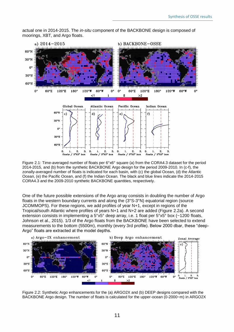
The synthetic in-situ datasets consist of sub-surface vertical profiles of temperature and salinity from mooring platforms, eXpendable BathyThermographs (XBTs), and Argo floats, which have been extracted from the CORA 4.1 in-situ database distributed by CMEMS In-situ TAC (Cabanes et al. 2013; Szekely et al. 2016). Following discussions with mooring networks, the mooring sampling during the year 2015 has been chosen to represent the mooring sampling for the 3-yr OSSE period (B. Bourlès and S. Cravatte, personal communication) as one of the most representative period of the Global Tropical Moored Buoy Array (www.pmel.noaa.gov/gtmba). The 2013-2015 drifters sampling is considered for the OSSE (P. Poli, personal communication). The synthetic Argo data for the BACKBONE system have been built based on the time and date location of Argo profiles during the period 2009-2011. In order to design a ”homogeneous” Argo sampling, approaching 1 float per 3°x3° square, float trajectories have been removed in the well-sampled Kuroshio region, or added in the low-sampled Tropical/South Atlantic region. More concretely, trajectories from floats deployed in the Kuroshio region (10°N-45°N; 120°E-150°E) in 2010-2011 have been arbitrarily removed. In the Tropical/South Atlantic region (south of 20°N), for a given date, half of the Argo distribution of the day of the following year has been added (i.e., the OSSE Argo trajectories of January 1, 2009 are equivalent to the actual Argo trajectories of January 1, 2010, plus half of the floats of the actual Argo trajectories of January, 1, 2011 in the tropical/south Atlantic). In Figure 2.1 (bottom panels), the time-averaged number of Argo floats, expressed as equivalent number per 3° x 3 ° square, is shown for the actual period 2014-2015, and for the synthetic BACKBONE configuration. The zonally-averaged number of floats for each basin demonstrates the more ”homogeneous” feature of the synthetic design compared with the
Synthesis of OSSE results
11
actual one in 2014-2015. The in-situ component of the BACKBONE design is composed of moorings, XBT, and Argo floats.
Figure 2.1: Time-averaged number of floats per 6°x6° square (a) from the CORA4.3 dataset for the period 2014-2015, and (b) from the synthetic BACKBONE Argo design for the period 2009-2010. In (c-f), the zonally-averaged number of floats is indicated for each basin, with (c) the global Ocean, (d) the Atlantic Ocean, (e) the Pacific Ocean, and (f) the Indian Ocean. The black and blue lines indicate the 2014-2015 CORA4.3 and the 2009-2010 synthetic BACKBONE quantities, respectively.
One of the future possible extensions of the Argo array consists in doubling the number of Argo floats in the western boundary currents and along the (3°S-3°N) equatorial region (source JCOMMOPS). For these regions, we add profiles of year N+1, except in regions of the Tropical/south Atlantic where profiles of years N+1 and N+2 are added (Figure 2.2a). A second extension consists in implementing a 5°x5° deep array, i.e. 1 float per 5°x5° box (~1200 floats, Johnson et al., 2015). 1/3 of the Argo floats from the BACKBONE have been selected to extend measurements to the bottom (5500m), monthly (every 3rd profile). Below 2000 dbar, these “deep-Argo” floats are extracted at the model depths.
Figure 2.2: Synthetic Argo enhancements for the (a) ARGO2X and (b) DEEP designs compared with the BACKBONE Argo design. The number of floats is calculated for the upper-ocean (0-2000~m) in ARGO2X
Synthesis of OSSE results
12
per 6°x6° square, and for the deeper ocean (below 2000~m) in DEEP per 5°x5° square. In (c), the zonally-averaged number of floats of the DEEP_ARGO design is indicated for the global Ocean.
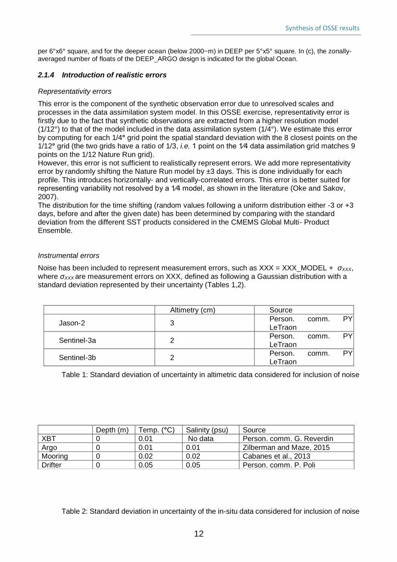
2.1.4 Introduction of realistic errors
Representativity errors
This error is the component of the synthetic observation error due to unresolved scales and processes in the data assimilation system model. In this OSSE exercise, representativity error is firstly due to the fact that synthetic observations are extracted from a higher resolution model (1/12°) to that of the model included in the data assimilation system (1/4°). We estimate this error by computing for each 1/4° grid point the spatial standard deviation with the 8 closest points on the 1/12° grid (the two grids have a ratio of 1/3, i.e. 1 point on the 1⁄4 data assimilation grid matches 9 points on the 1/12 Nature Run grid). However, this error is not sufficient to realistically represent errors. We add more representativity error by randomly shifting the Nature Run model by ±3 days. This is done individually for each profile. This introduces horizontally- and vertically-correlated errors. This error is better suited for representing variability not resolved by a 1⁄4 model, as shown in the literature (Oke and Sakov, 2007). The distribution for the time shifting (random values following a uniform distribution either -3 or +3 days, before and after the given date) has been determined by comparing with the standard deviation from the different SST products considered in the CMEMS Global Multi- Product Ensemble.
Instrumental errors
Noise has been included to represent measurement errors, such as XXX = XXX_MODEL + σXXX, where σXXX are measurement errors on XXX, defined as following a Gaussian distribution with a standard deviation represented by their uncertainty (Tables 1,2).
Altimetry (cm) Source
Jason-2 3 Person. comm. PY LeTraon
Sentinel-3a 2 Person. comm. PY LeTraon
Sentinel-3b 2 Person. comm. PY LeTraon
Table 1: Standard deviation of uncertainty in altimetric data considered for inclusion of noise
Table 2: Standard deviation in uncertainty of the in-situ data considered for inclusion of noise
Depth (m) Temp. (°C) Salinity (psu) Source
XBT 0 0.01 No data Person. comm. G. Reverdin
Argo 0 0.01 0.01 Zilberman and Maze, 2015
Mooring 0 0.02 0.02 Cabanes et al., 2013
Drifter 0 0.05 0.05 Person. comm. P. Poli
Synthesis of OSSE results
13
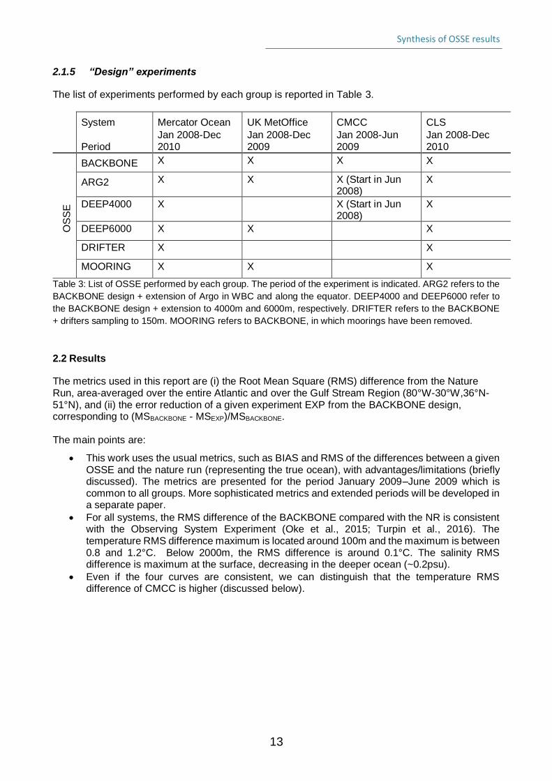
2.1.5 “Design” experiments
The list of experiments performed by each group is reported in Table 3.
• • System • Mercator Ocean • UK MetOffice • CMCC • CLS
• • Period
• Jan 2008-Dec 2010
• Jan 2008-Dec 2009
• Jan 2008-Jun 2009
• Jan 2008-Dec 2010
OS
SE
• BACKBONE • X • X • X • X
• ARG2 • X • X • X (Start in Jun 2008)
• X
• DEEP4000 • X • • X (Start in Jun 2008)
• X
• DEEP6000 • X • X • • X
• DRIFTER • X • • • X
• MOORING • X • X • • X
Table 3: List of OSSE performed by each group. The period of the experiment is indicated. ARG2 refers to the
BACKBONE design + extension of Argo in WBC and along the equator. DEEP4000 and DEEP6000 refer to
the BACKBONE design + extension to 4000m and 6000m, respectively. DRIFTER refers to the BACKBONE
+ drifters sampling to 150m. MOORING refers to BACKBONE, in which moorings have been removed.
2.2 Results
The metrics used in this report are (i) the Root Mean Square (RMS) difference from the Nature Run, area-averaged over the entire Atlantic and over the Gulf Stream Region (80°W-30°W,36°N-51°N), and (ii) the error reduction of a given experiment EXP from the BACKBONE design, corresponding to (MSBACKBONE - MSEXP)/MSBACKBONE. The main points are:
• This work uses the usual metrics, such as BIAS and RMS of the differences between a given OSSE and the nature run (representing the true ocean), with advantages/limitations (briefly discussed). The metrics are presented for the period January 2009–June 2009 which is common to all groups. More sophisticated metrics and extended periods will be developed in a separate paper.
• For all systems, the RMS difference of the BACKBONE compared with the NR is consistent with the Observing System Experiment (Oke et al., 2015; Turpin et al., 2016). The temperature RMS difference maximum is located around 100m and the maximum is between 0.8 and 1.2°C. Below 2000m, the RMS difference is around 0.1°C. The salinity RMS difference is maximum at the surface, decreasing in the deeper ocean (~0.2psu).
• Even if the four curves are consistent, we can distinguish that the temperature RMS difference of CMCC is higher (discussed below).
Synthesis of OSSE results
14
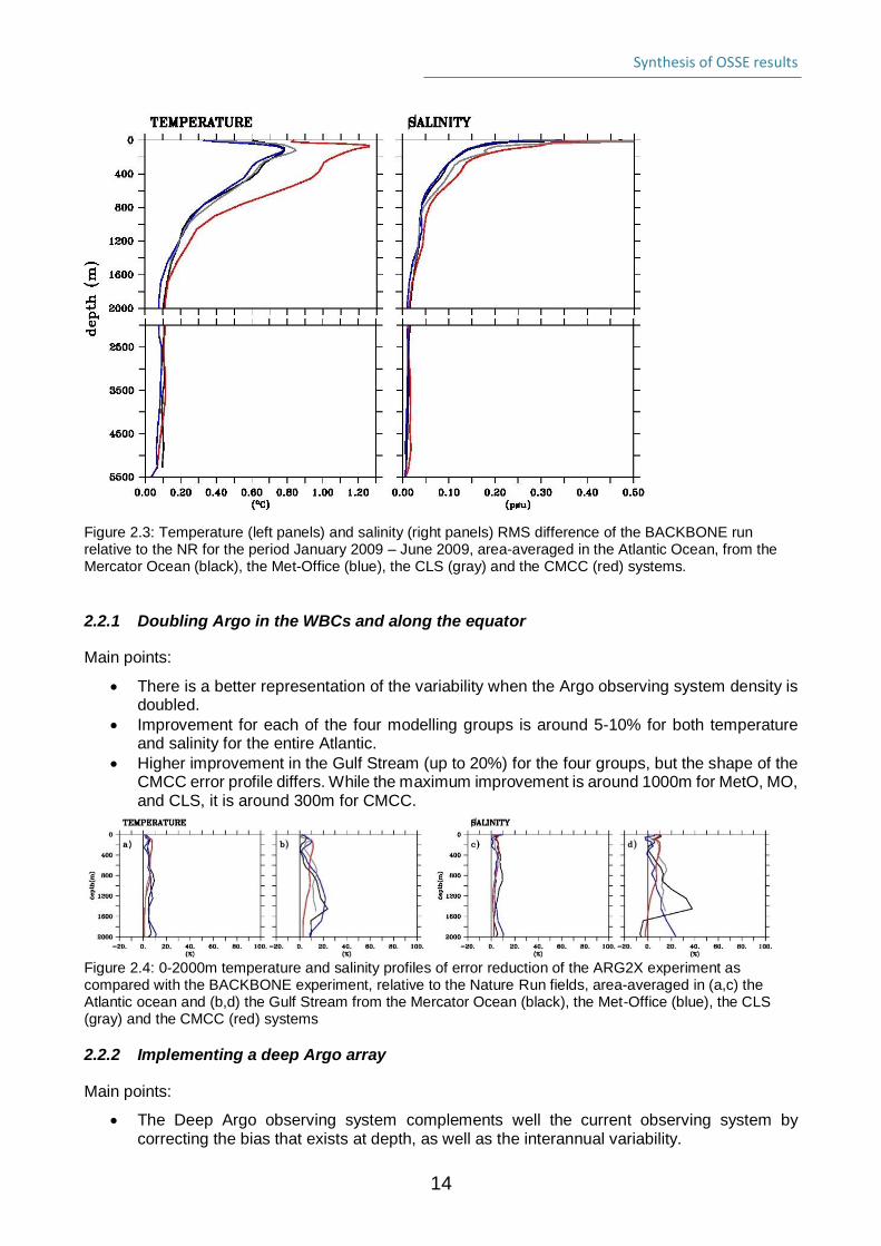
Figure 2.3: Temperature (left panels) and salinity (right panels) RMS difference of the BACKBONE run relative to the NR for the period January 2009 – June 2009, area-averaged in the Atlantic Ocean, from the Mercator Ocean (black), the Met-Office (blue), the CLS (gray) and the CMCC (red) systems.
2.2.1 Doubling Argo in the WBCs and along the equator
Main points:
• There is a better representation of the variability when the Argo observing system density is doubled.
• Improvement for each of the four modelling groups is around 5-10% for both temperature and salinity for the entire Atlantic.
• Higher improvement in the Gulf Stream (up to 20%) for the four groups, but the shape of the CMCC error profile differs. While the maximum improvement is around 1000m for MetO, MO, and CLS, it is around 300m for CMCC.
Figure 2.4: 0-2000m temperature and salinity profiles of error reduction of the ARG2X experiment as compared with the BACKBONE experiment, relative to the Nature Run fields, area-averaged in (a,c) the Atlantic ocean and (b,d) the Gulf Stream from the Mercator Ocean (black), the Met-Office (blue), the CLS (gray) and the CMCC (red) systems
2.2.2 Implementing a deep Argo array
Main points:
• The Deep Argo observing system complements well the current observing system by correcting the bias that exists at depth, as well as the interannual variability.
Synthesis of OSSE results
15
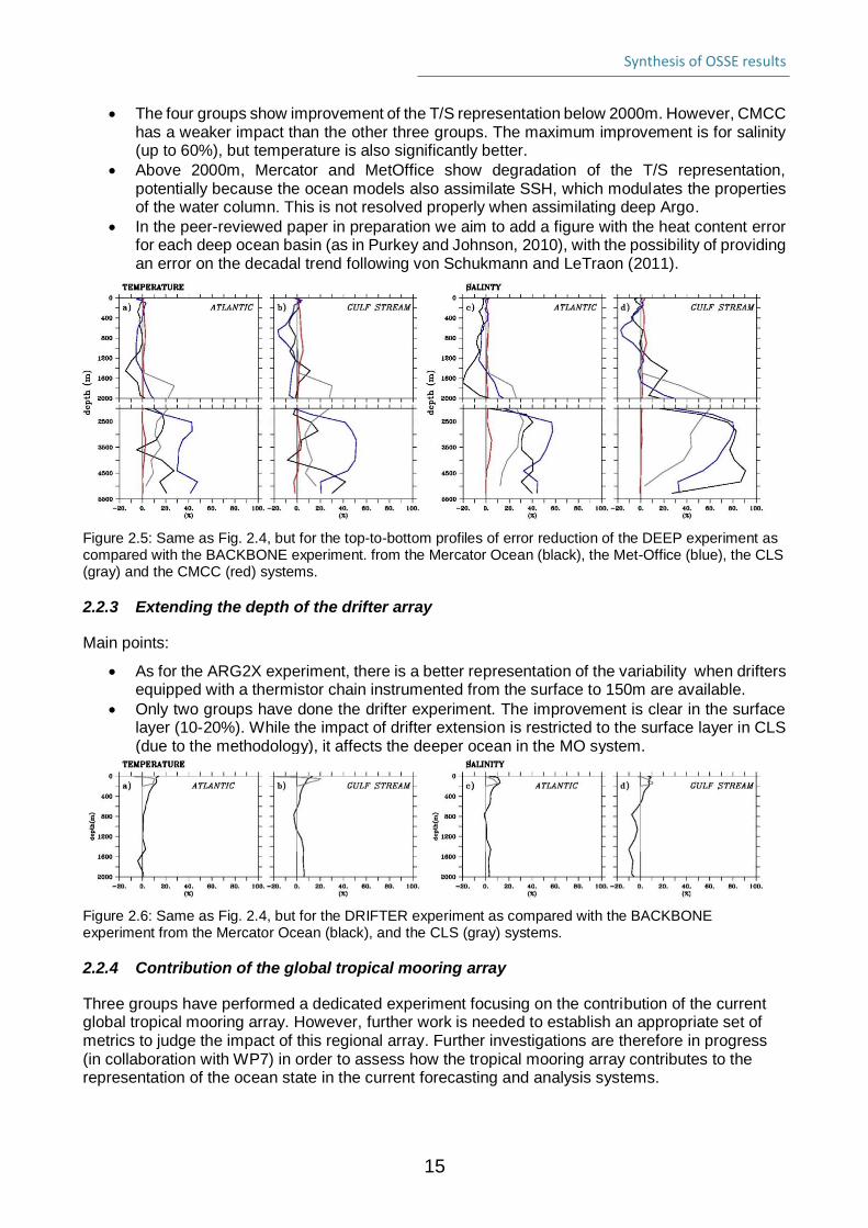
• The four groups show improvement of the T/S representation below 2000m. However, CMCC has a weaker impact than the other three groups. The maximum improvement is for salinity (up to 60%), but temperature is also significantly better.
• Above 2000m, Mercator and MetOffice show degradation of the T/S representation, potentially because the ocean models also assimilate SSH, which modulates the properties of the water column. This is not resolved properly when assimilating deep Argo.
• In the peer-reviewed paper in preparation we aim to add a figure with the heat content error for each deep ocean basin (as in Purkey and Johnson, 2010), with the possibility of providing an error on the decadal trend following von Schukmann and LeTraon (2011).
Figure 2.5: Same as Fig. 2.4, but for the top-to-bottom profiles of error reduction of the DEEP experiment as compared with the BACKBONE experiment. from the Mercator Ocean (black), the Met-Office (blue), the CLS (gray) and the CMCC (red) systems.
2.2.3 Extending the depth of the drifter array
Main points:
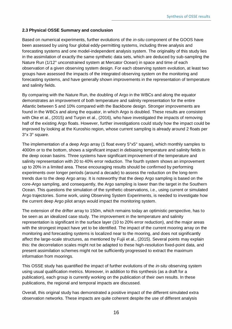
• As for the ARG2X experiment, there is a better representation of the variability when drifters equipped with a thermistor chain instrumented from the surface to 150m are available.
• Only two groups have done the drifter experiment. The improvement is clear in the surface layer (10-20%). While the impact of drifter extension is restricted to the surface layer in CLS (due to the methodology), it affects the deeper ocean in the MO system.
Figure 2.6: Same as Fig. 2.4, but for the DRIFTER experiment as compared with the BACKBONE experiment from the Mercator Ocean (black), and the CLS (gray) systems.
2.2.4 Contribution of the global tropical mooring array
Three groups have performed a dedicated experiment focusing on the contribution of the current global tropical mooring array. However, further work is needed to establish an appropriate set of metrics to judge the impact of this regional array. Further investigations are therefore in progress (in collaboration with WP7) in order to assess how the tropical mooring array contributes to the representation of the ocean state in the current forecasting and analysis systems.
Synthesis of OSSE results
16
2.3 Physical OSSE Summary and conclusion
Based on numerical experiments, further evolutions of the in-situ component of the GOOS have
been assessed by using four global eddy-permitting systems, including three analysis and
forecasting systems and one model-independent analysis system. The originality of this study lies
in the assimilation of exactly the same synthetic data sets, which are deduced by sub-sampling the
Nature Run (1/12° unconstrained system at Mercator Ocean) in space and time of each
observation of a given observing system design. For each observing system evolution, at least two
groups have assessed the impacts of the integrated observing system on the monitoring and
forecasting systems, and have generally shown improvements in the representation of temperature
and salinity fields.
By comparing with the Nature Run, the doubling of Argo in the WBCs and along the equator
demonstrates an improvement of both temperature and salinity representation for the entire
Atlantic between 5 and 10% compared with the Backbone design. Stronger improvements are
found in the WBCs and along the equator, in which Argo is doubled. These results are consistent
with Oke et al., (2015) and Turpin et al., (2016), who have investigated the impacts of removing
half of the existing Argo floats. However, further investigations could study how the impact could be
improved by looking at the Kuroshio region, whose current sampling is already around 2 floats per
3°x 3° square.
The implementation of a deep Argo array (1 float every 5°x5° square), which monthly samples to
4000m or to the bottom, shows a significant impact in debiasing temperature and salinity fields in
the deep ocean basins. Three systems have significant improvement of the temperature and
salinity representation with 20 to 40% error reduction. The fourth system shows an improvement
up to 20% in a limited area. These encouraging results should be confirmed by performing
experiments over longer periods (around a decade) to assess the reduction on the long-term
trends due to the deep Argo array. It is noteworthy that the deep Argo sampling is based on the
core-Argo sampling, and consequently, the Argo sampling is lower than the target in the Southern
Ocean. This questions the simulation of the synthetic observations, i.e., using current or simulated
Argo trajectories. Some work, using Observing System Experiments, is needed to investigate how
the current deep Argo pilot arrays would impact the monitoring system.
The extension of the drifter array to 150m, which remains today an optimistic perspective, has to
be seen as an idealized case study. The improvement in the temperature and salinity
representation is significant in the surface layer (10 to 20% error reduction), and the major areas
with the strongest impact have yet to be identified. The impact of the current mooring array on the
monitoring and forecasting systems is localized near to the mooring, and does not significantly
affect the large-scale structures, as mentioned by Fujii et al., (2015). Several points may explain
this: the decorrelation scales might not be adapted to these high-resolution fixed-point data, and
present assimilation schemes might not be sufficiently progressed to extract the maximum
information from moorings.
This OSSE study has quantified the impact of further evolutions of the in-situ observing system
using usual qualification metrics. Moreover, in addition to this synthesis (as a draft for a
publication), each group is currently working on the publication of their own results. In these
publications, the regional and temporal impacts are discussed.
Overall, this original study has demonstrated a positive impact of the different simulated extra
observation networks. These impacts are quite coherent despite the use of different analysis
Synthesis of OSSE results
17
systems, although the CMCC system behavior looks slightly different from the others. The interest
of this work also resides in identifying the limitations of the method in order to overcome these
issues in future OSSEs. As mentioned previously, the results are model-dependent and it is
assumed that impacts of the observing system components evolve following the development of
the monitoring and forecasting system, including time and space resolution. Moreover, the
experiments rely on the performance of the Nature Run, and any improvement of the free
simulation, especially below the surface layer, should improve the results. The systems are tuned
for a specific observation network and require time to adapt to a new one. A longer period of OSSE
is thus required to obtain more significant and robust statistics, especially in the deeper ocean.
Global experiments involving different instruments and measurements can make the investigation
of local processes at different time and space scales difficult, however. All these aspects could be
addressed in a future exercise.
In conclusion, a coordinated effort from European forecasting centers carried out within the H2020
AtlantOS project has provided consistent information about observation impacts on monitoring and
forecasting systems concerning the evolution of the in-situ component of the GOOS. In the
continuity of the GODAE Ocean View activities, this work tackles the assessment of observation
impacts in monitoring and forecasting systems, and can be seen as a step further toward the
guidance of sampling strategy in the preparation of the OceanObs’19 conference. However, the
present work is a first step toward future coordinated impact studies, in which the development of
assimilation schemes and progress in numerical models should significantly improve the
robustness of results, and enable the use of more sophisticated process metrics.
Synthesis of OSSE results
18
2.4 A complementary Observing System Experiment (OSE)
ECMWF carried out and explored a number of Observing System Experiments (OSEs) in order to identify important ocean regions and observations for analyses and seasonal forecasts. OSEs are complementary to the OSSEs above in that they take an existing data assimilating analysis system (using real observations) and test the impact of removing certain observation streams. Additionally, statistical tools have been developed to explore the sensitivity of errors in seasonal predictions over Europe to errors in ocean initial conditions. The currently operational ocean reanalysis system 5 (ORAS5; Zuo et al. 2018) forms the basis for the OSE work. ORAS5 is a coupled ocean-sea-ice reanalysis and uses the NEMOv3.4 ocean model and the LIM2 sea ice model. Assimilation method (3D Var FGAT), resolution (¼ degree horizontal with 75 levels) and boundary forcing (ERA-Interim) are the same as in ORAP5 (Zuo et al. 2017), but some components have been improved, including use of more up-to-date observational data sets. ORAS5 uses the recently released quality-controlled EN4 (Good et al. 2013) in-situ dataset with better vertical resolution and extended coverage than the previous version EN3 used in ORAP5. The altimeter sea-level data has also been updated to use the latest version (DUACS2014) from AVISO. The SST product before 2008 has also been changed and in ORAS5 is based on the Met Office Hadley Centre sea ice and sea surface temperature data set, version 2 (Titchner and Rayner 2014). One reference assimilation run using all available observations (REF) and four OSEs have been carried out for the period 1993-2015, using a low-resolution (1 degree horizontal, 42 levels) version of ORAS5. For the different OSEs the following observing system components have been removed globally: 1) Argo float observations (NoArgo), 2) Moored buoys data (including Tropical Mooring arrays) (NoMooring), 3) XBT/MBT and CTD observations (NoXBT), 4) all in-situ observations (Argo, moored buoys, XBT/MBT, CTD; NoInsitu). SST-nudging and sea level assimilation were switched on in all OSEs, but not bias correction. Results are described in Section 2.4.1. To statistically derive the sensitivities of errors in seasonal forecasts from the errors in ocean initial conditions, Canonical Correlation Analysis (CCA) has been implemented and applied to ECMWF’s new seasonal prediction system SEAS5, which became operational in November 2017. SEAS5 has the same ocean model resolution as ORAS5 and uses ocean initial conditions from this reanalysis. The atmosphere model in SEAS5 runs on an O320 (~36km) horizontal resolution. This contribution seizes SEAS5 re-forecasts covering the period 1981-2014 with a 25 member ensemble. A description of CCA and results from its application to SEAS5 are presented in Section 2.4.2 Implementation of CCA and its application to ECMWF’s seasonal prediction also serves as preparation for AtlantOS task 7.4, where seasonal predictions initialized from the OSEs described above will be assessed with this tool.
2.4.1 Results from OSEs
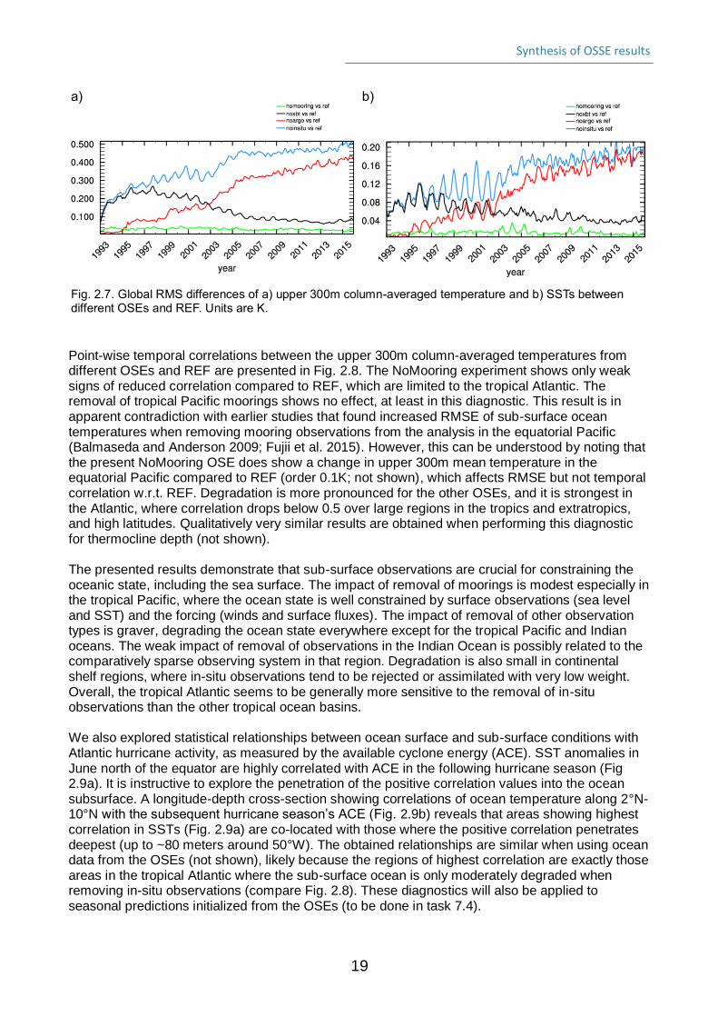
The temporal evolution of global RMS differences in the upper 300m column-averaged temperatures between the four OSEs and REF are depicted in Fig. 2.7a. Not surprisingly, average differences are largest for the NoArgo experiment and smallest for the NoMooring experiment, reflecting the very different numbers of observations and spatial coverage of the two observing systems. The increase of the differences for NoArgo reflects primarily the increasing number of Argo observations with time, while the opposite is the case for the NoXBT experiment. Removal of sub-surface observations also affects SSTs. This can be seen from Fig. 2.7b which shows the temporal evolution of global RMS differences of SSTs between the four OSEs and REF. Qualitatively, the behaviour is very similar to that found for sub-surface temperatures (Fig. 2.7a) but with a stronger signal in the annual cycle before ~2003, when the observational coverage was much stronger in the North Hemisphere. Global RMS differences are sizeable and reach 0.2K for the NoInsitu experiment. This result demonstrates that sub-surface information is useful also for constraining SSTs, despite the nudging of SSTs.
Synthesis of OSSE results
19
a)
b)
Fig. 2.7. Global RMS differences of a) upper 300m column-averaged temperature and b) SSTs between different OSEs and REF. Units are K.
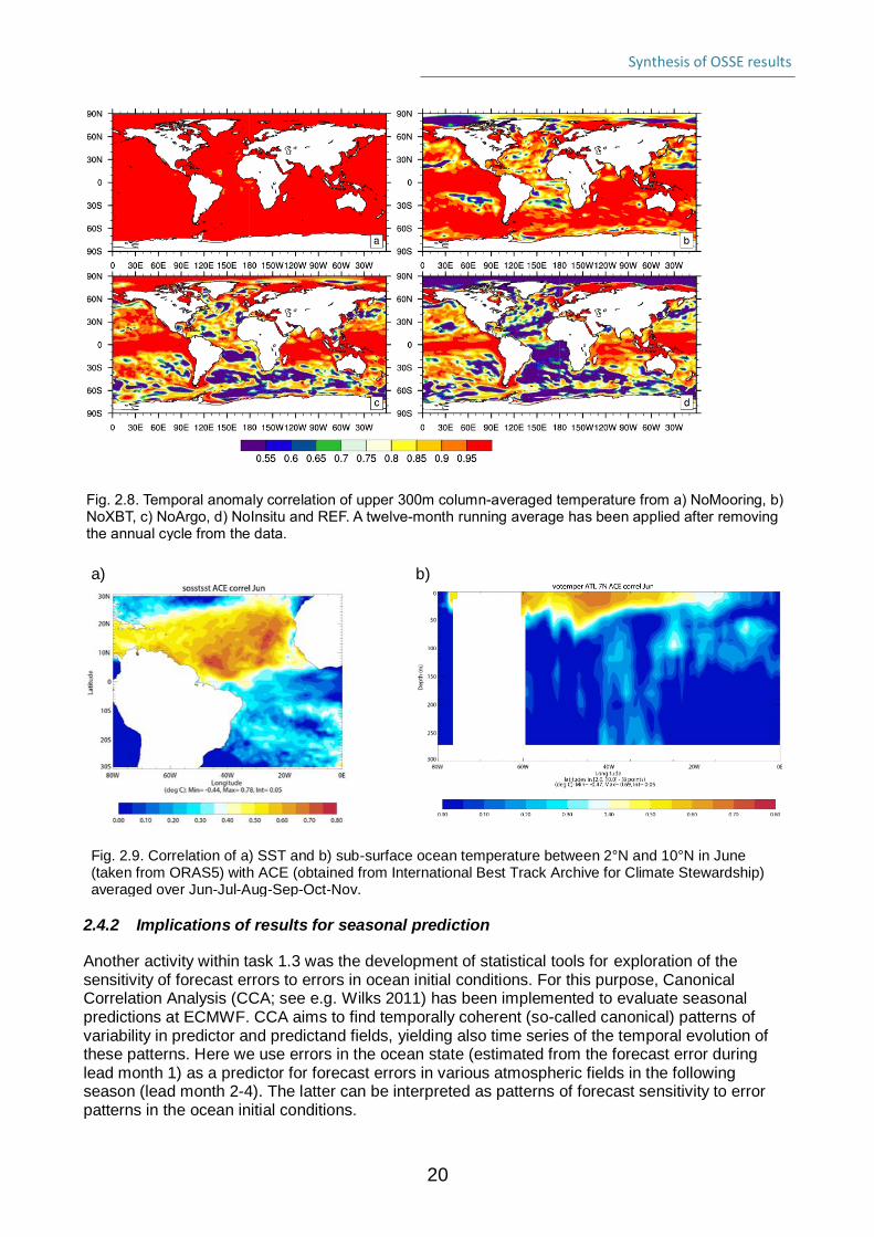
Point-wise temporal correlations between the upper 300m column-averaged temperatures from different OSEs and REF are presented in Fig. 2.8. The NoMooring experiment shows only weak signs of reduced correlation compared to REF, which are limited to the tropical Atlantic. The removal of tropical Pacific moorings shows no effect, at least in this diagnostic. This result is in apparent contradiction with earlier studies that found increased RMSE of sub-surface ocean temperatures when removing mooring observations from the analysis in the equatorial Pacific (Balmaseda and Anderson 2009; Fujii et al. 2015). However, this can be understood by noting that the present NoMooring OSE does show a change in upper 300m mean temperature in the equatorial Pacific compared to REF (order 0.1K; not shown), which affects RMSE but not temporal correlation w.r.t. REF. Degradation is more pronounced for the other OSEs, and it is strongest in the Atlantic, where correlation drops below 0.5 over large regions in the tropics and extratropics, and high latitudes. Qualitatively very similar results are obtained when performing this diagnostic for thermocline depth (not shown). The presented results demonstrate that sub-surface observations are crucial for constraining the oceanic state, including the sea surface. The impact of removal of moorings is modest especially in the tropical Pacific, where the ocean state is well constrained by surface observations (sea level and SST) and the forcing (winds and surface fluxes). The impact of removal of other observation types is graver, degrading the ocean state everywhere except for the tropical Pacific and Indian oceans. The weak impact of removal of observations in the Indian Ocean is possibly related to the comparatively sparse observing system in that region. Degradation is also small in continental shelf regions, where in-situ observations tend to be rejected or assimilated with very low weight. Overall, the tropical Atlantic seems to be generally more sensitive to the removal of in-situ observations than the other tropical ocean basins. We also explored statistical relationships between ocean surface and sub-surface conditions with Atlantic hurricane activity, as measured by the available cyclone energy (ACE). SST anomalies in June north of the equator are highly correlated with ACE in the following hurricane season (Fig 2.9a). It is instructive to explore the penetration of the positive correlation values into the ocean subsurface. A longitude-depth cross-section showing correlations of ocean temperature along 2°N-10°N with the subsequent hurricane season’s ACE (Fig. 2.9b) reveals that areas showing highest correlation in SSTs (Fig. 2.9a) are co-located with those where the positive correlation penetrates deepest (up to ~80 meters around 50°W). The obtained relationships are similar when using ocean data from the OSEs (not shown), likely because the regions of highest correlation are exactly those areas in the tropical Atlantic where the sub-surface ocean is only moderately degraded when removing in-situ observations (compare Fig. 2.8). These diagnostics will also be applied to seasonal predictions initialized from the OSEs (to be done in task 7.4).
Synthesis of OSSE results
20
Fig. 2.8. Temporal anomaly correlation of upper 300m column-averaged temperature from a) NoMooring, b) NoXBT, c) NoArgo, d) NoInsitu and REF. A twelve-month running average has been applied after removing the annual cycle from the data.
a)
b)
Fig. 2.9. Correlation of a) SST and b) sub-surface ocean temperature between 2°N and 10°N in June (taken from ORAS5) with ACE (obtained from International Best Track Archive for Climate Stewardship) averaged over Jun-Jul-Aug-Sep-Oct-Nov.
2.4.2 Implications of results for seasonal prediction
Another activity within task 1.3 was the development of statistical tools for exploration of the sensitivity of forecast errors to errors in ocean initial conditions. For this purpose, Canonical Correlation Analysis (CCA; see e.g. Wilks 2011) has been implemented to evaluate seasonal predictions at ECMWF. CCA aims to find temporally coherent (so-called canonical) patterns of variability in predictor and predictand fields, yielding also time series of the temporal evolution of these patterns. Here we use errors in the ocean state (estimated from the forecast error during lead month 1) as a predictor for forecast errors in various atmospheric fields in the following season (lead month 2-4). The latter can be interpreted as patterns of forecast sensitivity to error patterns in the ocean initial conditions.
Synthesis of OSSE results
21
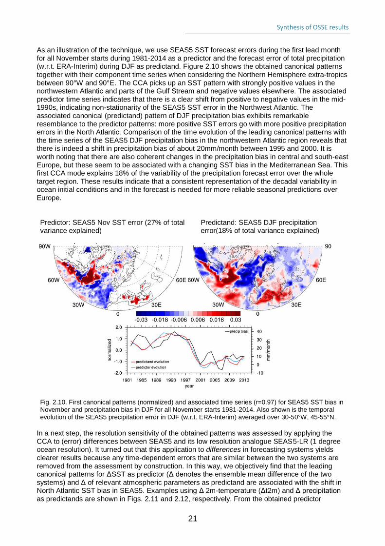
As an illustration of the technique, we use SEAS5 SST forecast errors during the first lead month for all November starts during 1981-2014 as a predictor and the forecast error of total precipitation (w.r.t. ERA-Interim) during DJF as predictand. Figure 2.10 shows the obtained canonical patterns together with their component time series when considering the Northern Hemisphere extra-tropics between 90°W and 90°E. The CCA picks up an SST pattern with strongly positive values in the northwestern Atlantic and parts of the Gulf Stream and negative values elsewhere. The associated predictor time series indicates that there is a clear shift from positive to negative values in the mid-1990s, indicating non-stationarity of the SEAS5 SST error in the Northwest Atlantic. The associated canonical (predictand) pattern of DJF precipitation bias exhibits remarkable resemblance to the predictor patterns: more positive SST errors go with more positive precipitation errors in the North Atlantic. Comparison of the time evolution of the leading canonical patterns with the time series of the SEAS5 DJF precipitation bias in the northwestern Atlantic region reveals that there is indeed a shift in precipitation bias of about 20mm/month between 1995 and 2000. It is worth noting that there are also coherent changes in the precipitation bias in central and south-east Europe, but these seem to be associated with a changing SST bias in the Mediterranean Sea. This first CCA mode explains 18% of the variability of the precipitation forecast error over the whole target region. These results indicate that a consistent representation of the decadal variability in ocean initial conditions and in the forecast is needed for more reliable seasonal predictions over Europe. Predictor: SEAS5 Nov SST error (27% of total variance explained)
Predictand: SEAS5 DJF precipitation error(18% of total variance explained)
Fig. 2.10. First canonical patterns (normalized) and associated time series (r=0.97) for SEAS5 SST bias in November and precipitation bias in DJF for all November starts 1981-2014. Also shown is the temporal evolution of the SEAS5 precipitation error in DJF (w.r.t. ERA-Interim) averaged over 30-50°W, 45-55°N.
In a next step, the resolution sensitivity of the obtained patterns was assessed by applying the CCA to (error) differences between SEAS5 and its low resolution analogue SEAS5-LR (1 degree ocean resolution). It turned out that this application to differences in forecasting systems yields clearer results because any time-dependent errors that are similar between the two systems are removed from the assessment by construction. In this way, we objectively find that the leading canonical patterns for ΔSST as predictor (Δ denotes the ensemble mean difference of the two systems) and Δ of relevant atmospheric parameters as predictand are associated with the shift in North Atlantic SST bias in SEAS5. Examples using Δ 2m-temperature (Δt2m) and Δ precipitation as predictands are shown in Figs. 2.11 and 2.12, respectively. From the obtained predictor
Synthesis of OSSE results
22
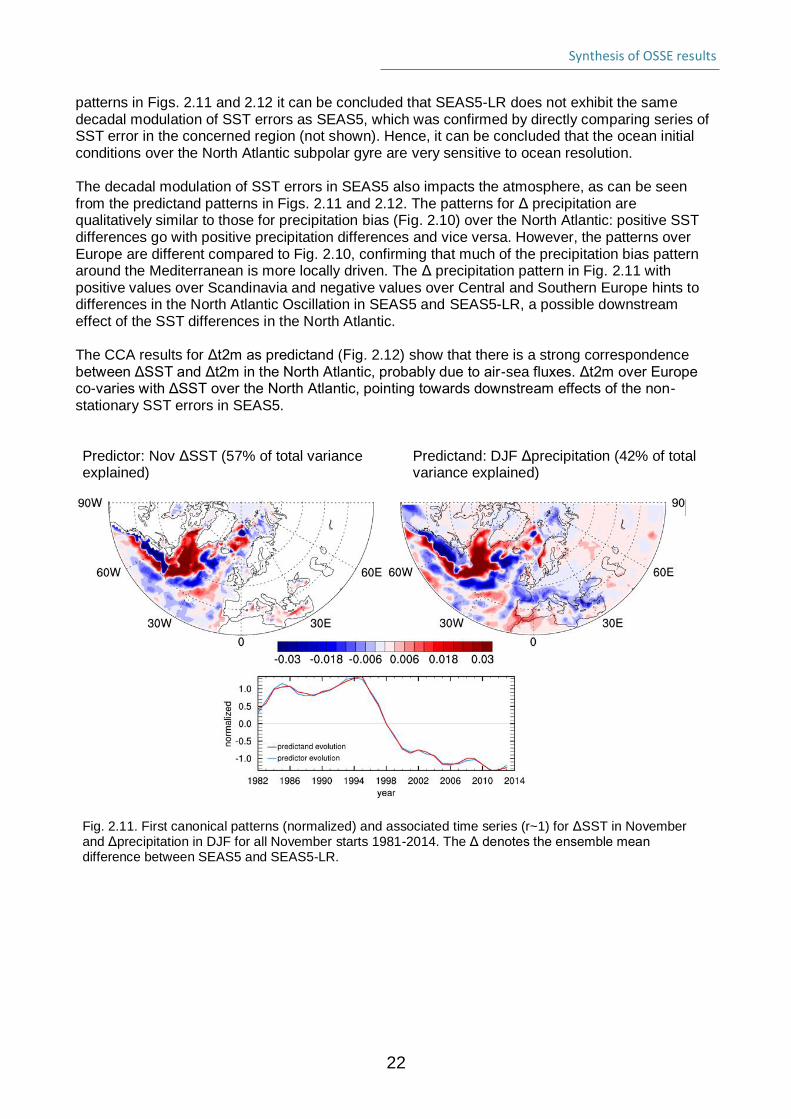
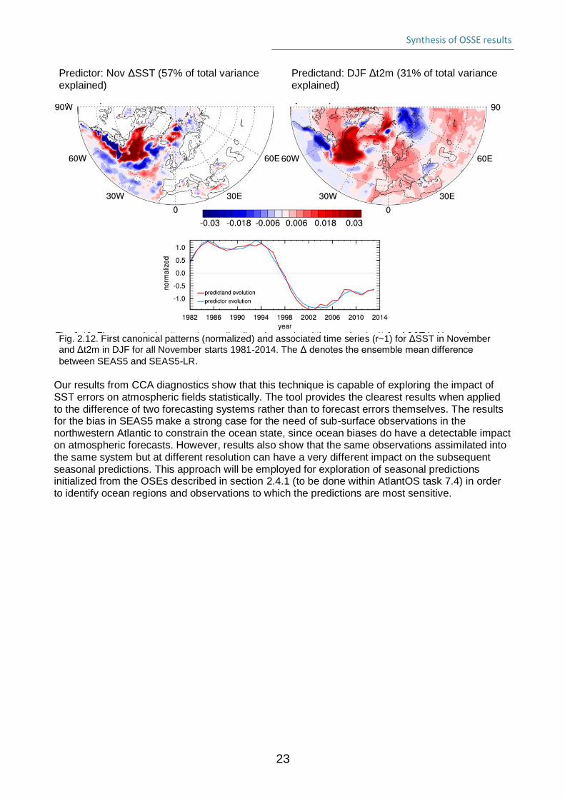
patterns in Figs. 2.11 and 2.12 it can be concluded that SEAS5-LR does not exhibit the same decadal modulation of SST errors as SEAS5, which was confirmed by directly comparing series of SST error in the concerned region (not shown). Hence, it can be concluded that the ocean initial conditions over the North Atlantic subpolar gyre are very sensitive to ocean resolution. The decadal modulation of SST errors in SEAS5 also impacts the atmosphere, as can be seen from the predictand patterns in Figs. 2.11 and 2.12. The patterns for Δ precipitation are qualitatively similar to those for precipitation bias (Fig. 2.10) over the North Atlantic: positive SST differences go with positive precipitation differences and vice versa. However, the patterns over Europe are different compared to Fig. 2.10, confirming that much of the precipitation bias pattern around the Mediterranean is more locally driven. The Δ precipitation pattern in Fig. 2.11 with positive values over Scandinavia and negative values over Central and Southern Europe hints to differences in the North Atlantic Oscillation in SEAS5 and SEAS5-LR, a possible downstream effect of the SST differences in the North Atlantic. The CCA results for Δt2m as predictand (Fig. 2.12) show that there is a strong correspondence between ΔSST and Δt2m in the North Atlantic, probably due to air-sea fluxes. Δt2m over Europe co-varies with ΔSST over the North Atlantic, pointing towards downstream effects of the non-stationary SST errors in SEAS5. Predictor: Nov ΔSST (57% of total variance explained)
Predictand: DJF Δprecipitation (42% of total variance explained)
Fig. 2.11. First canonical patterns (normalized) and associated time series (r~1) for ΔSST in November and Δprecipitation in DJF for all November starts 1981-2014. The Δ denotes the ensemble mean difference between SEAS5 and SEAS5-LR.
Synthesis of OSSE results
23
Predictor: Nov ΔSST (57% of total variance explained)
Predictand: DJF Δt2m (31% of total variance explained)
Fig. 2.12. First canonical patterns (normalized) and associated time series (r~1) for ΔSST in November and Δt2m in DJF for all November starts 1981-2014. The Δ denotes the ensemble mean difference
between SEAS5 and SEAS5-LR. Our results from CCA diagnostics show that this technique is capable of exploring the impact of SST errors on atmospheric fields statistically. The tool provides the clearest results when applied to the difference of two forecasting systems rather than to forecast errors themselves. The results for the bias in SEAS5 make a strong case for the need of sub-surface observations in the northwestern Atlantic to constrain the ocean state, since ocean biases do have a detectable impact on atmospheric forecasts. However, results also show that the same observations assimilated into the same system but at different resolution can have a very different impact on the subsequent seasonal predictions. This approach will be employed for exploration of seasonal predictions initialized from the OSEs described in section 2.4.1 (to be done within AtlantOS task 7.4) in order to identify ocean regions and observations to which the predictions are most sensitive.
Synthesis of OSSE results
24
3. Biogeochemical OSSEs 3.1 Introduction The major development in the in-situ observing system over the next few years will be Biogeochemical-Argo (Johnson and Claustre, 2016), hereafter BGC-Argo, which builds on the success of Argo. It is planned to have a sustained global array of approximately 1000 BGC-Argo floats, each measuring six core variables: oxygen concentration, nitrate concentration, pH, chlorophyll-a concentration, suspended particles, and downwelling irradiance. These are likely to be based on core Argo float technology, profiling from 2000m depth to the surface every ten days, and transmitting the observed data in near-real-time via Iridium. Due to regional programmes such as the Southern Ocean Carbon and Climate Observations and Modeling project (SOCCOM), there are already around 300 operational floats measuring one or more biogeochemical variables, but a global array measuring all variables has yet to be established. Most state-of-the-art biogeochemical forecasting and reanalysis systems only assimilate ocean colour data (Gehlen et al., 2015; Ciavatta et al., 2014). Due to the sparsity of observations, assimilation of in-situ biogeochemical data has largely been restricted to 1D models or specific research applications (e.g. Anderson et al., 2000). Meanwhile, assimilation of physical variables has been known to degrade biogeochemical simulations, due to imperfect assimilation schemes that result in spurious impacts on vertical mixing, to which biogeochemical variables are particularly sensitive (Park et al., 2018; Raghukumar et al., 2015). However, many centres plan to exploit the increasing availability of BGC-Argo data in their systems. Two different data assimilation-based methodologies have been developed and compared, by CNRS/IGE and the Met Office. Each has tested two different potential BGC-Argo array distributions. The first represents the target BGC-Argo array of around 1000 floats, approximately equivalent to having biogeochemical sensors on a quarter of existing Argo floats. The second represents an array of around 4000 floats, equivalent to having biogeochemical sensors on all existing Argo floats. Experiments combining assimilation of BGC-Argo and satellite ocean colour arrays have been performed to assess their combined value. Subsections 3.2 and 3.3 below give an overview of the CNRS/IGE and Met Office experiments and results, followed by a brief inter-comparison and summary of conclusions and recommendations from these experiments in subsection 3.4. More detailed accounts of each group’s experiments are provided in Appendices to this report , and these will form the basis of two peer-reviewed publications. A third publication will provide more detailed inter-comparison, regional assessment for the Atlantic, and recommendations for the observation and assimilation communities. Further work by CNRS/IGE, focussing on regional design studies, is being conducted as part of WP5 of AtlantOS. Finally, in subsection 3.5, we describe an independent study by CNRS/LSCE which uses a statistical modelling approach to determine what would be an effective observing network to monitor surface pCO2. 3.2 CNRS/IGE experiments The effect of uncertainties due to various biogeochemical model imperfections (e.g. simplified biology, unresolved biological diversity, unresolved scales) can play a key role in estimating the dynamical behaviors of ocean ecosystems. To better represent these model uncertainties, a recent study (Garnier et al. 2016) investigated the use of an ensemble Monte Carlo approach based on the inclusion of stochastic processes. This study showed the potential of such an approach by explicitly simulating the joint effects of uncertain biological parameters and unresolved scales into a coupled physical-biogeochemical model in a 1/4° North Atlantic configuration. The ensemble was able to simulate surface chlorophyll distributions consistent with satellite ocean colour data, where
Synthesis of OSSE results
25
information brought by each ensemble member was necessary to correctly represent the spatial features of ocean colour. As part of AtlantOS, and building on the experience acquired from this study, the CNRS/IGE team aimed to assess the impacts of two potential BGC-Argo arrays on this ensemble simulation, as well as their complementarity with existing satellite ocean colour observations. However, classical deterministic verification tools used in OSSEs, such as root-mean-square error metrics, are not suitable for evaluating ensemble-based experiments which require a probabilistic approach. For this purpose, we developed an integrated ensemble-based probability score methodology to perform a new type of OSSE which relies on estimating two probabilistic properties: the reliability and the resolution, as suggested by Candille et al., (2007). The first property tests whether the ensemble with assimilation is consistent compared to a true state (known as the verification), which is a necessary but not sufficient condition to assess if the observing system adds value or not. The second property aims to assess the actual gain of information brought by the observing system, allowing the evaluation of different deployment scenarios. Here, two verification tools (one for each property) are presented to emphasize four experiments (see below), while a thorough description of the verification methodology is presented in Appendix C Note that a major limitation of this approach is its computational burden, and therefore the difficulty of applying this to a forecast context. As a first attempt, and to reduce the numerical cost, we applied this new methodology to a single date (15/04/2005), in order to assess the following basic deployment scenarios:
• BGC-Argo on 1/4 of the nominal Argo array • BGC-Argo on the full nominal Argo array • daily satellite ocean colour data and BGC-Argo on 1/4 of the nominal array • daily satellite ocean colour data and BGC-Argo on nominal array
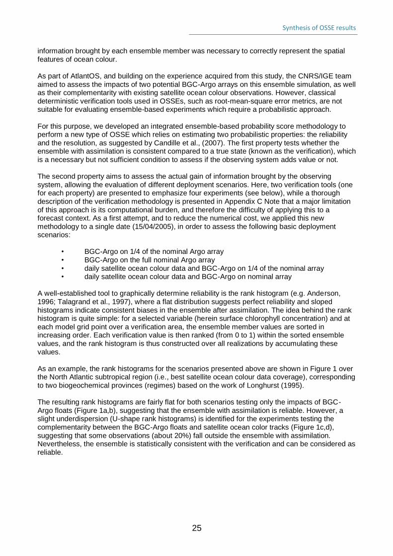
A well-established tool to graphically determine reliability is the rank histogram (e.g. Anderson, 1996; Talagrand et al., 1997), where a flat distribution suggests perfect reliability and sloped histograms indicate consistent biases in the ensemble after assimilation. The idea behind the rank histogram is quite simple: for a selected variable (herein surface chlorophyll concentration) and at each model grid point over a verification area, the ensemble member values are sorted in increasing order. Each verification value is then ranked (from 0 to 1) within the sorted ensemble values, and the rank histogram is thus constructed over all realizations by accumulating these values. As an example, the rank histograms for the scenarios presented above are shown in Figure 1 over the North Atlantic subtropical region (i.e., best satellite ocean colour data coverage), corresponding to two biogeochemical provinces (regimes) based on the work of Longhurst (1995). The resulting rank histograms are fairly flat for both scenarios testing only the impacts of BGC-Argo floats (Figure 1a,b), suggesting that the ensemble with assimilation is reliable. However, a slight underdispersion (U-shape rank histograms) is identified for the experiments testing the complementarity between the BGC-Argo floats and satellite ocean color tracks (Figure 1c,d), suggesting that some observations (about 20%) fall outside the ensemble with assimilation. Nevertheless, the ensemble is statistically consistent with the verification and can be considered as reliable.
Synthesis of OSSE results
26
Figure 3.1
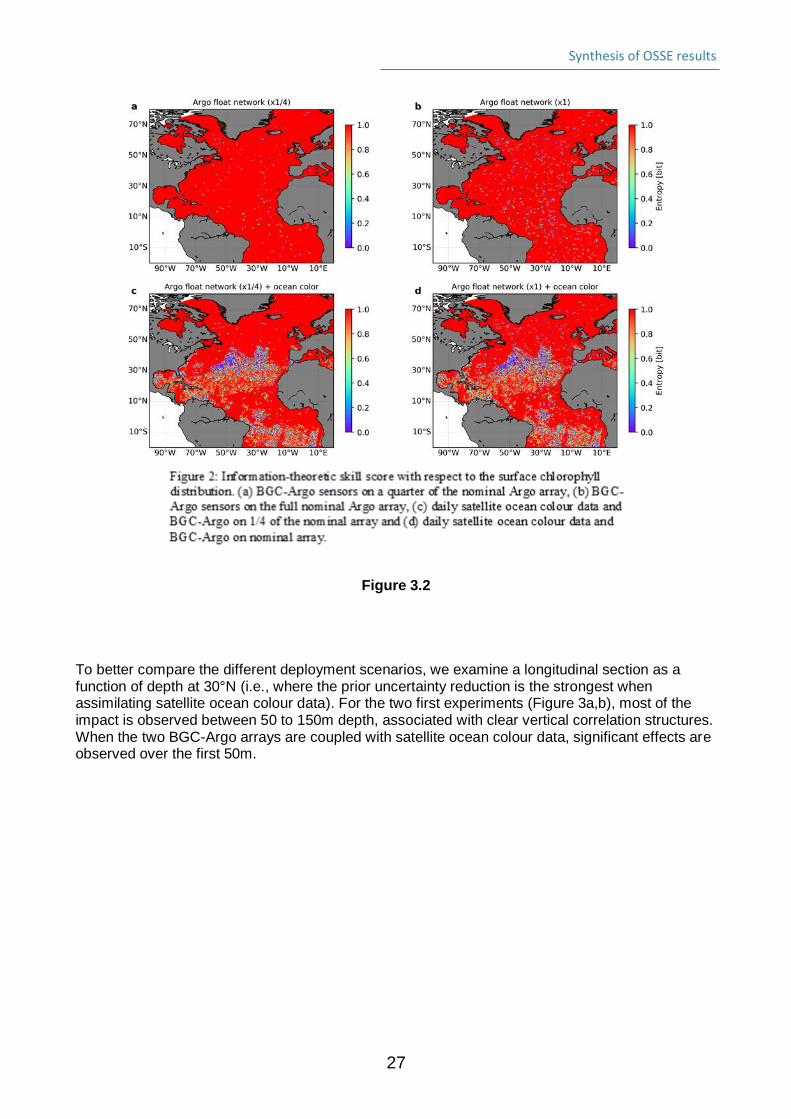
A probabilistic scoring measure using information theory (i.e., based on the amount of data compression) is used here to assess the resolution property. This measure, called ignorance by Roulston and Smith (2002), allows the discrimination of tested observing scenarios without averaging over a verification area, unlike more common probabilistic tools such as the continuous ranked probability score (CRPS; Hersbach, 2000). Appendix C gives more details about how this information-theoretic metric based on entropy is calculated. Here, only key results are presented to emphasize the advantages of this metric, which appears to be a useful tool in evaluation of probabilistic OSSEs. The surface entropy maps with respect to chlorophyll (Figure 2) show a reduction of entropy (i.e., uncertainty) where observations have been assimilated. For the two first experiments (Figure 2a,b), the spread of the prior ensemble is reduced locally at the positions of the synthetic BGC-Argo floats (colored dots). For the two experiments including both BGC-Argo arrays and ocean colour data (Figure 2c,d), the prior uncertainty is mostly reduced within a zonal band across the North Atlantic Basin at around 30°N, matching with the best coverage of satellite ocean color tracks. As expected, the strongest reduction of prior uncertainty at the surface is observed with the densest observing system (i.e. existing satellite ocean color data and BGC-Argo on nominal array), especially where the use of satellite systems is limited due to cloudy conditions.
Synthesis of OSSE results
27
Figure 3.2
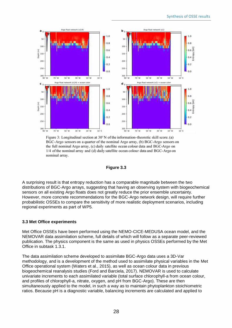
To better compare the different deployment scenarios, we examine a longitudinal section as a function of depth at 30°N (i.e., where the prior uncertainty reduction is the strongest when assimilating satellite ocean colour data). For the two first experiments (Figure 3a,b), most of the impact is observed between 50 to 150m depth, associated with clear vertical correlation structures. When the two BGC-Argo arrays are coupled with satellite ocean colour data, significant effects are observed over the first 50m.
Synthesis of OSSE results
28
Figure 3.3
A surprising result is that entropy reduction has a comparable magnitude between the two distributions of BGC-Argo arrays, suggesting that having an observing system with biogeochemical sensors on all existing Argo floats does not greatly reduce the prior ensemble uncertainty. However, more concrete recommendations for the BGC-Argo network design, will require further probabilistic OSSEs to compare the sensitivity of more realistic deployment scenarios, including regional experiments as part of WP5. 3.3 Met Office experiments Met Office OSSEs have been performed using the NEMO-CICE-MEDUSA ocean model, and the NEMOVAR data assimilation scheme, full details of which will follow as a separate peer-reviewed publication. The physics component is the same as used in physics OSSEs performed by the Met Office in subtask 1.3.1. The data assimilation scheme developed to assimilate BGC-Argo data uses a 3D-Var methodology, and is a development of the method used to assimilate physical variables in the Met Office operational system (Waters et al., 2015), as well as ocean colour data in previous biogeochemical reanalysis studies (Ford and Barciela, 2017). NEMOVAR is used to calculate univariate increments to each assimilated variable (total surface chlorophyll-a from ocean colour, and profiles of chlorophyll-a, nitrate, oxygen, and pH from BGC-Argo). These are then simultaneously applied to the model, in such a way as to maintain phytoplankton stoichiometric ratios. Because pH is a diagnostic variable, balancing increments are calculated and applied to
Synthesis of OSSE results
29
dissolved inorganic carbon (DIC) and alkalinity, using a similar method to the partial pressure of carbon dioxide (pCO2) assimilation scheme of While et al. (2012). A non-assimilative nature run was performed using standard configurations of the modelling system at 1/4° resolution, forced at the surface by fluxes from the ERA-Interim reanalysis (Dee et al., 2011). This was used to provide the model truth. An equivalent non-assimilative control run was then performed using a perturbed version of the model. Atmospheric forcing was changed to the JRA-55 reanalysis (Kobayashi et al., 2015), physics and biogeochemistry initial conditions were altered, and different NEMO and MEDUSA parameter settings were used. Both the nature and control run were run from 1 January 2008 to 31 December 2009, with the first year treated as spin-up. Experiments have also been performed in which only the biogeochemistry was perturbed, not the physics, to examine the impact of circulation errors. The results do not alter the conclusions presented here, so they are omitted for brevity, but will be detailed in forthcoming publications. A series of assimilation experiments were then performed, assimilating synthetic observations sampled from the nature run, into the version of the model used for the control run. These were each run for one year from 1 January to 31 December 2009. Experiments assimilated different combinations of synthetic ocean colour and BGC-Argo data, simulating having biogeochemical sensors on either all or a quarter of the existing Argo array. Ocean colour observation locations were taken from the European Space Agency Climate Change Initiative (ESA CCI) product available through the Copernicus Marine Environment Monitoring Service (CMEMS). BGC-Argo float trajectories were based on the “backbone” Argo array produced for the physics OSSEs in Subtask 1.3.1. For the experiments with biogeochemical sensors on a quarter of the floats, these trajectories were subsampled based on the last two digits of the float ID. Following the method used in Subtask 1.3.1, the observations were sampled from the nature run, with measurement and representation error added. For measurement error, unbiased Gaussian noise was added with standard deviations taken from the literature (Boss et al., 2008; Johnson et al., 2017). For representation error, the difference between the truth value and the value three days before or after (chosen at random) was added. As in the CNRS/IGE experiments (see Section 2.3.2), the following scenarios have been tested:
• BGC-Argo on 1/4 of the nominal Argo array • BGC-Argo on the full nominal Argo array • daily satellite ocean colour data and BGC-Argo on 1/4 of the nominal array • daily satellite ocean colour data and BGC-Argo on nominal array
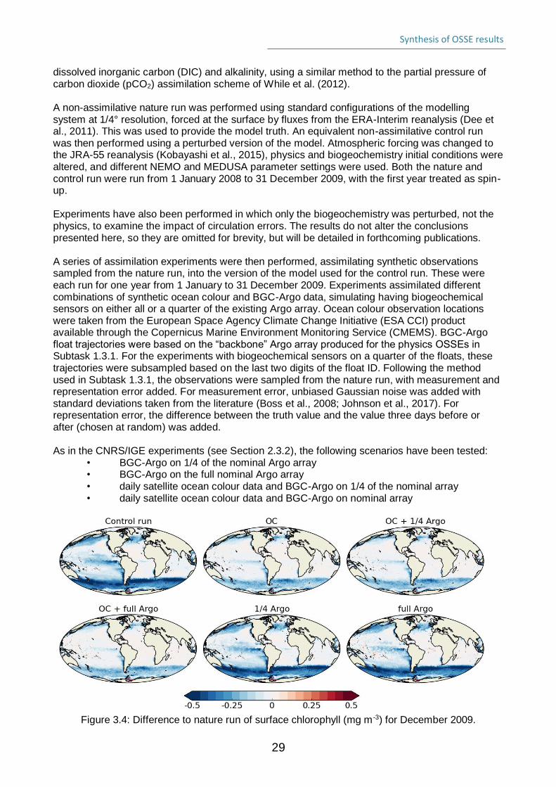
Figure 3.4: Difference to nature run of surface chlorophyll (mg m -3) for December 2009.
Synthesis of OSSE results
30
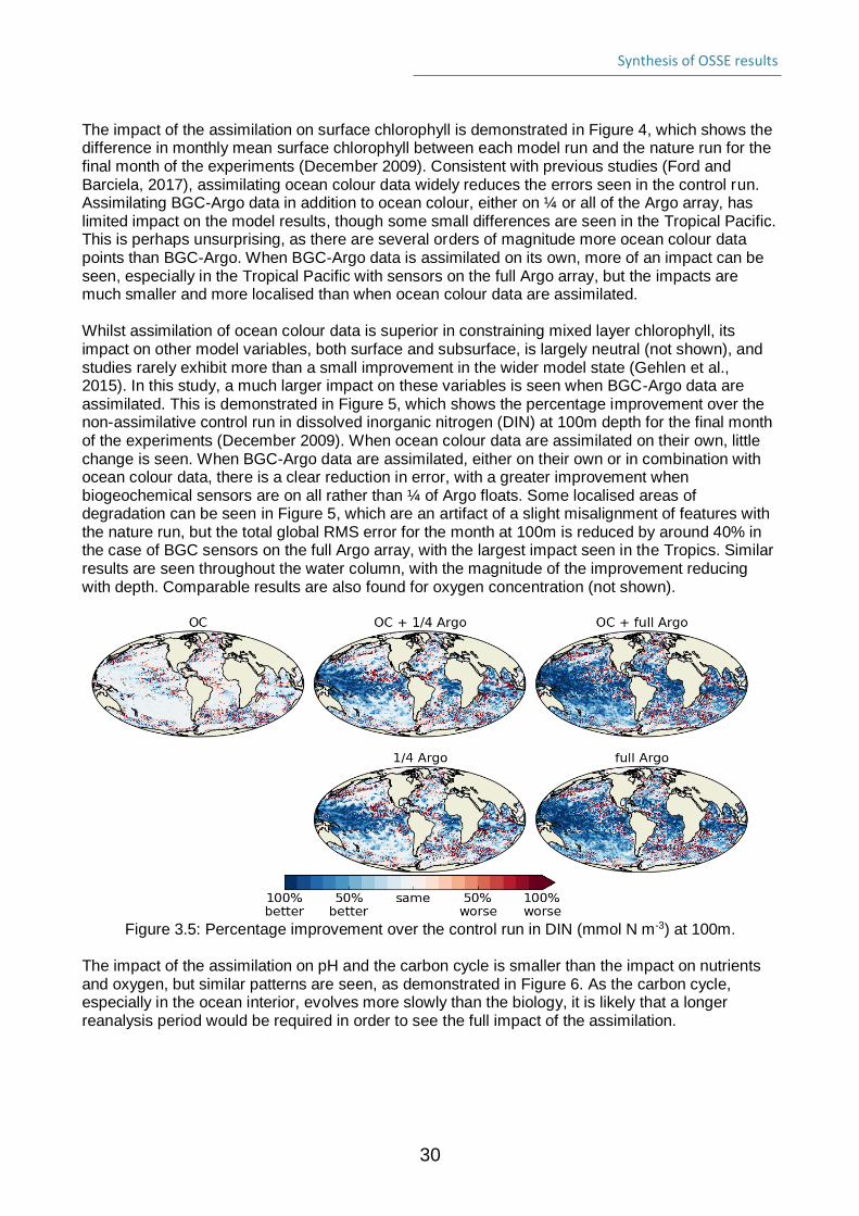
The impact of the assimilation on surface chlorophyll is demonstrated in Figure 4, which shows the difference in monthly mean surface chlorophyll between each model run and the nature run for the final month of the experiments (December 2009). Consistent with previous studies (Ford and Barciela, 2017), assimilating ocean colour data widely reduces the errors seen in the control run. Assimilating BGC-Argo data in addition to ocean colour, either on ¼ or all of the Argo array, has limited impact on the model results, though some small differences are seen in the Tropical Pacific. This is perhaps unsurprising, as there are several orders of magnitude more ocean colour data points than BGC-Argo. When BGC-Argo data is assimilated on its own, more of an impact can be seen, especially in the Tropical Pacific with sensors on the full Argo array, but the impacts are much smaller and more localised than when ocean colour data are assimilated. Whilst assimilation of ocean colour data is superior in constraining mixed layer chlorophyll, its impact on other model variables, both surface and subsurface, is largely neutral (not shown), and studies rarely exhibit more than a small improvement in the wider model state (Gehlen et al., 2015). In this study, a much larger impact on these variables is seen when BGC-Argo data are assimilated. This is demonstrated in Figure 5, which shows the percentage improvement over the non-assimilative control run in dissolved inorganic nitrogen (DIN) at 100m depth for the final month of the experiments (December 2009). When ocean colour data are assimilated on their own, little change is seen. When BGC-Argo data are assimilated, either on their own or in combination with ocean colour data, there is a clear reduction in error, with a greater improvement when biogeochemical sensors are on all rather than ¼ of Argo floats. Some localised areas of degradation can be seen in Figure 5, which are an artifact of a slight misalignment of features with the nature run, but the total global RMS error for the month at 100m is reduced by around 40% in the case of BGC sensors on the full Argo array, with the largest impact seen in the Tropics. Similar results are seen throughout the water column, with the magnitude of the improvement reducing with depth. Comparable results are also found for oxygen concentration (not shown).
Figure 3.5: Percentage improvement over the control run in DIN (mmol N m-3) at 100m.
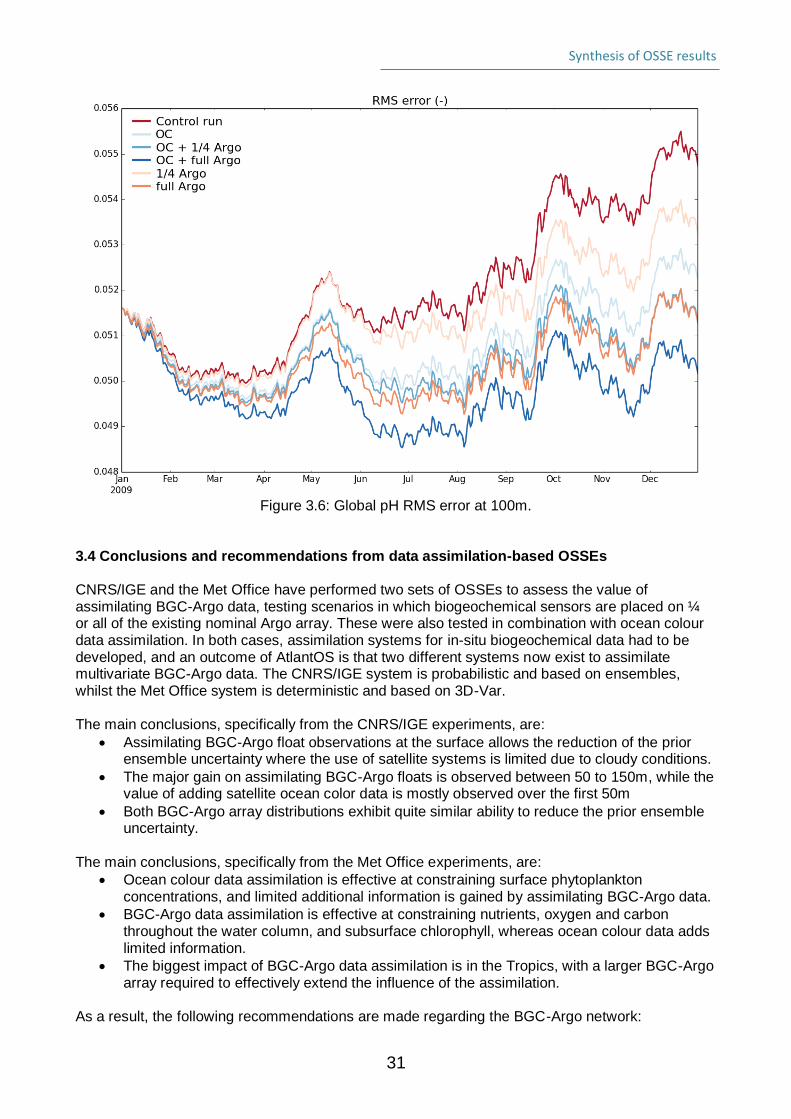
The impact of the assimilation on pH and the carbon cycle is smaller than the impact on nutrients and oxygen, but similar patterns are seen, as demonstrated in Figure 6. As the carbon cycle, especially in the ocean interior, evolves more slowly than the biology, it is likely that a longer reanalysis period would be required in order to see the full impact of the assimilation.
Synthesis of OSSE results
31
Figure 3.6: Global pH RMS error at 100m.
3.4 Conclusions and recommendations from data assimilation-based OSSEs CNRS/IGE and the Met Office have performed two sets of OSSEs to assess the value of assimilating BGC-Argo data, testing scenarios in which biogeochemical sensors are placed on ¼ or all of the existing nominal Argo array. These were also tested in combination with ocean colour data assimilation. In both cases, assimilation systems for in-situ biogeochemical data had to be developed, and an outcome of AtlantOS is that two different systems now exist to assimilate multivariate BGC-Argo data. The CNRS/IGE system is probabilistic and based on ensembles, whilst the Met Office system is deterministic and based on 3D-Var. The main conclusions, specifically from the CNRS/IGE experiments, are:
• Assimilating BGC-Argo float observations at the surface allows the reduction of the prior ensemble uncertainty where the use of satellite systems is limited due to cloudy conditions.
• The major gain on assimilating BGC-Argo floats is observed between 50 to 150m, while the value of adding satellite ocean color data is mostly observed over the first 50m
• Both BGC-Argo array distributions exhibit quite similar ability to reduce the prior ensemble uncertainty.
The main conclusions, specifically from the Met Office experiments, are:
• Ocean colour data assimilation is effective at constraining surface phytoplankton concentrations, and limited additional information is gained by assimilating BGC-Argo data.
• BGC-Argo data assimilation is effective at constraining nutrients, oxygen and carbon throughout the water column, and subsurface chlorophyll, whereas ocean colour data adds limited information.
• The biggest impact of BGC-Argo data assimilation is in the Tropics, with a larger BGC-Argo array required to effectively extend the influence of the assimilation.
As a result, the following recommendations are made regarding the BGC-Argo network:
Synthesis of OSSE results
32
• A BGC-Argo array of the target size (1000 floats) would provide data that could be usefully exploited to improve ocean biogeochemical reanalyses.
• BGC-Argo observations are complementary to ocean colour data, providing information that ocean colour data is unable to, but with more limited information about surface chlorophyll than ocean colour can provide.
• There is some evidence that a BGC-Argo array larger than the target size would allow the data assimilation to better constrain the models, but this evidence is based on immature assimilation capability, and may or may not still hold if more effective methods of exploiting the data are developed.
The following recommendations are made regarding the assimilation of BGC-Argo data:
• Assimilation of in-situ biogeochemical data is still to be improved, and developments to assimilation methods, as well as expanding observational coverage, are likely to yield benefits.
• As BGC-Argo data coverage is likely to remain relatively sparse compared with Argo data, assimilation methods which are specifically designed to work with sparse observational coverage (such as using empirical orthogonal functions or scale separation methods) may need to be considered.
• The biggest gains brought by assimilating BGC-Argo data appear to be subsurface, and combining assimilation of BGC-Argo and ocean colour data, in order to best constrain surface productivity and carbon fluxes, is likely to be a key challenge.
3.5 Identifying an optimal observing network to estimate the ocean carbon system using statistical models We explored a complementary approach to assessing design options for a future Atlantic scale observational carbon network, using statistical modelling techniques to enable the release of carbon system estimates at monthly and seasonal frequencies by combining data streams from various platforms. Experiments were carried out in a perfect model framework using output from an online-coupled physical-biogeochemical global ocean model at 1/4º nominal resolution (NEMO (OPA_LIM)-PISCES). The simulation covers the period 1958 to 2010; the last 3 years were retained for the design study. The output frequency of surface ocean fields was 5 days. Pseudo-observations were obtained by sub-sampling model output at sites of real-word observations. Surface ocean pCO2 was reconstructed from these pseudo-observations at basin scale by applying a non-linear feed forward neural network (FFNN) (Bishop, 1995; Rumelhart et al., 1988). Details of the method will be presented in a forthcoming dedicated paper (Sommer et al. in prep). The remainder of the section is structured into a first part presenting observing systems and observations, a second part briefly describing the statistical model, a third part introducing the design experiments and a final one dedicated to main results and perspectives. 3.5.1. Observing systems and real-world observations. Three observing systems were selected for the study, all providing in-situ measurements of carbonate system variables: (1) SOCAT database v5 (Bakker et al., 2016): SOCAT combines surface ocean measurements of fCO2 from multiple platforms and provides a good cover of the Northern Hemisphere. Data for the period 2001-2010 were used, representing ~60% of data in SOCAT database. (2) Argo profilers: Biogeochemical Argo floats are increasingly equipped with pH sensors allowing computation of pCO2 from pH and SST- based alkalinity. We considered Argo floats as being equipped with CO2 sensors for this design study. We used the network of Argo distributions
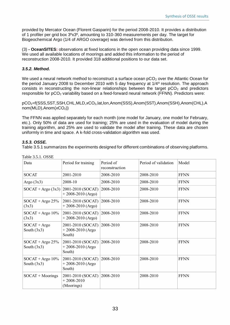
Synthesis of OSSE results
33
provided by Mercator Ocean (Florent Gasparin) for the period 2008-2010. It provides a distribution of 1 profiler per grid box 3ºx3º, amounting to 310-360 measurements per day. The target for Biogeochemical Argo (1/4 of ARGO coverage) was derived from this distribution. (3) - OceanSITES: observations at fixed locations in the open ocean providing data since 1999. We used all available locations of moorings and added this information to the period of reconstruction 2008-2010. It provided 318 additional positions to our data set. 3.5.2. Method. We used a neural network method to reconstruct a surface ocean pCO2 over the Atlantic Ocean for the period January 2008 to December 2010 with 5 day frequency at 1/4º resolution. The approach consists in reconstructing the non-linear relationships between the target pCO2 and predictors responsible for pCO2 variability based on a feed-forward neural network (FFNN). Predictors were: pCO2=f(SSS,SST,SSH,CHL,MLD,xCO2,lat,lon,Anom(SSS),Anom(SST),Anom(SSH),Anom(CHL),Anom(MLD),Anom(xCO2)) The FFNN was applied separately for each month (one model for January, one model for February, etc.). Only 50% of data are used for training; 25% are used in the evaluation of model during the training algorithm, and 25% are used to validate the model after training. These data are chosen uniformly in time and space. A k-fold cross-validation algorithm was used. 3.5.3. OSSE. Table 3.5.1 summarizes the experiments designed for different combinations of observing platforms. Table 3.5.1. OSSE
Data Period for training Period of
reconstruction
Period of validation Model
SOCAT 2001-2010 2008-2010 2008-2010 FFNN
Argo (3x3) 2008-10 2008-2010 2008-2010 FFNN
SOCAT + Argo (3x3) 2001-2010 (SOCAT)
+ 2008-2010 (Argo)
2008-2010 2008-2010 FFNN
SOCAT + Argo 25%
(3x3)
2001-2010 (SOCAT)
+ 2008-2010 (Argo)
2008-2010 2008-2010 FFNN
SOCAT + Argo 10%
(3x3)
2001-2010 (SOCAT)
+ 2008-2010 (Argo)
2008-2010 2008-2010 FFNN
SOCAT + Argo
South (3x3)
2001-2010 (SOCAT)
+ 2008-2010 (Argo
South)
2008-2010 2008-2010 FFNN
SOCAT + Argo 25%
South (3x3)
2001-2010 (SOCAT)
+ 2008-2010 (Argo
South)
2008-2010 2008-2010 FFNN
SOCAT + Argo 10%
South (3x3)
2001-2010 (SOCAT)
+ 2008-2010 (Argo
South)
2008-2010 2008-2010 FFNN
SOCAT + Moorings 2001-2010 (SOCAT)
+ 2008-2010
(Moorings)
2008-2010 2008-2010 FFNN
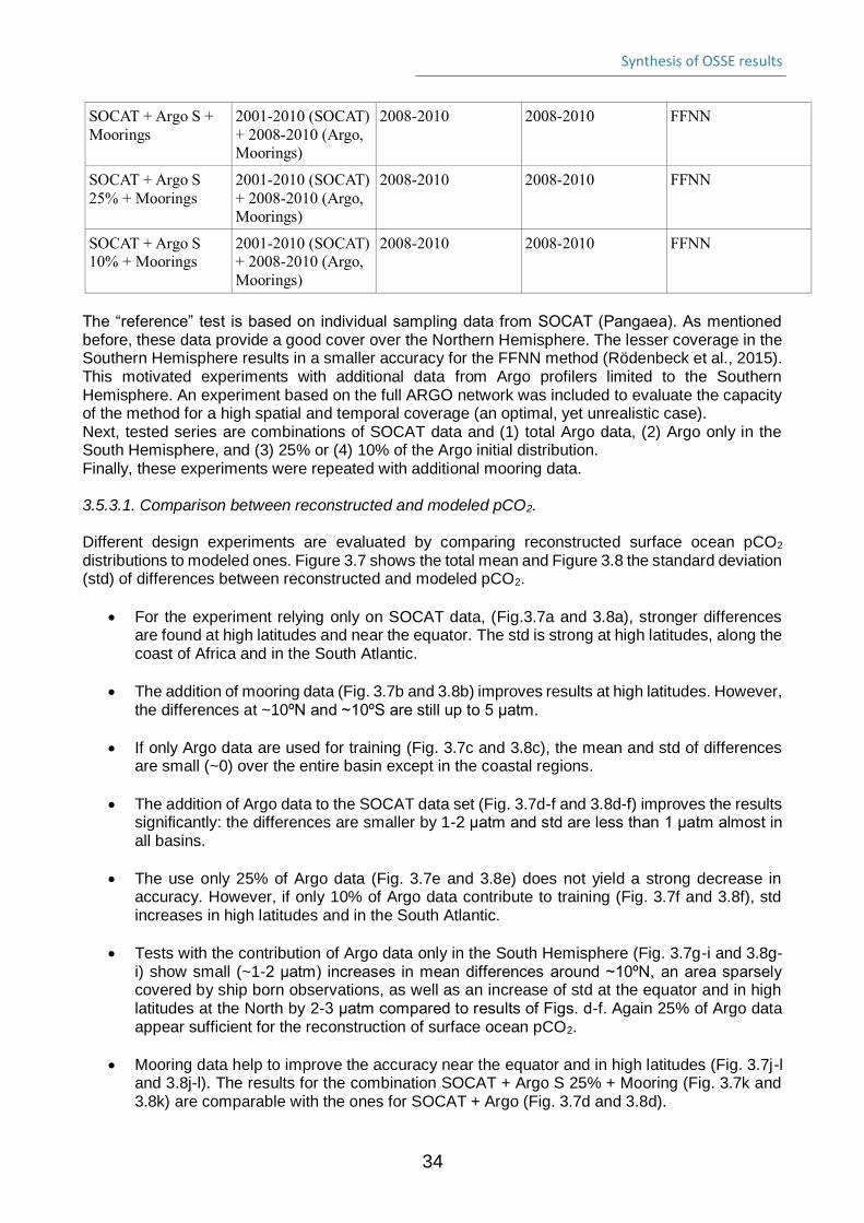
Synthesis of OSSE results
34
SOCAT + Argo S +
Moorings
2001-2010 (SOCAT)
+ 2008-2010 (Argo,
Moorings)
2008-2010 2008-2010 FFNN
SOCAT + Argo S
25% + Moorings
2001-2010 (SOCAT)
+ 2008-2010 (Argo,
Moorings)
2008-2010 2008-2010 FFNN
SOCAT + Argo S
10% + Moorings
2001-2010 (SOCAT)
+ 2008-2010 (Argo,
Moorings)
2008-2010 2008-2010 FFNN
The “reference” test is based on individual sampling data from SOCAT (Pangaea). As mentioned before, these data provide a good cover over the Northern Hemisphere. The lesser coverage in the Southern Hemisphere results in a smaller accuracy for the FFNN method (Rödenbeck et al., 2015). This motivated experiments with additional data from Argo profilers limited to the Southern Hemisphere. An experiment based on the full ARGO network was included to evaluate the capacity of the method for a high spatial and temporal coverage (an optimal, yet unrealistic case). Next, tested series are combinations of SOCAT data and (1) total Argo data, (2) Argo only in the South Hemisphere, and (3) 25% or (4) 10% of the Argo initial distribution. Finally, these experiments were repeated with additional mooring data. 3.5.3.1. Comparison between reconstructed and modeled pCO2. Different design experiments are evaluated by comparing reconstructed surface ocean pCO2 distributions to modeled ones. Figure 3.7 shows the total mean and Figure 3.8 the standard deviation (std) of differences between reconstructed and modeled pCO2.
• For the experiment relying only on SOCAT data, (Fig.3.7a and 3.8a), stronger differences are found at high latitudes and near the equator. The std is strong at high latitudes, along the coast of Africa and in the South Atlantic.
• The addition of mooring data (Fig. 3.7b and 3.8b) improves results at high latitudes. However, the differences at ~10ºN and ~10ºS are still up to 5 μatm.
• If only Argo data are used for training (Fig. 3.7c and 3.8c), the mean and std of differences are small (~0) over the entire basin except in the coastal regions.
• The addition of Argo data to the SOCAT data set (Fig. 3.7d-f and 3.8d-f) improves the results significantly: the differences are smaller by 1-2 μatm and std are less than 1 μatm almost in all basins.
• The use only 25% of Argo data (Fig. 3.7e and 3.8e) does not yield a strong decrease in accuracy. However, if only 10% of Argo data contribute to training (Fig. 3.7f and 3.8f), std increases in high latitudes and in the South Atlantic.
• Tests with the contribution of Argo data only in the South Hemisphere (Fig. 3.7g-i and 3.8g-i) show small (~1-2 μatm) increases in mean differences around ~10ºN, an area sparsely covered by ship born observations, as well as an increase of std at the equator and in high latitudes at the North by 2-3 μatm compared to results of Figs. d-f. Again 25% of Argo data appear sufficient for the reconstruction of surface ocean pCO2.
• Mooring data help to improve the accuracy near the equator and in high latitudes (Fig. 3.7j-l and 3.8j-l). The results for the combination SOCAT + Argo S 25% + Mooring (Fig. 3.7k and 3.8k) are comparable with the ones for SOCAT + Argo (Fig. 3.7d and 3.8d).

Synthesis of OSSE results
35
These results suggest that the combination of SOCAT + Argo S 25% + Mooring is an optimal variant.
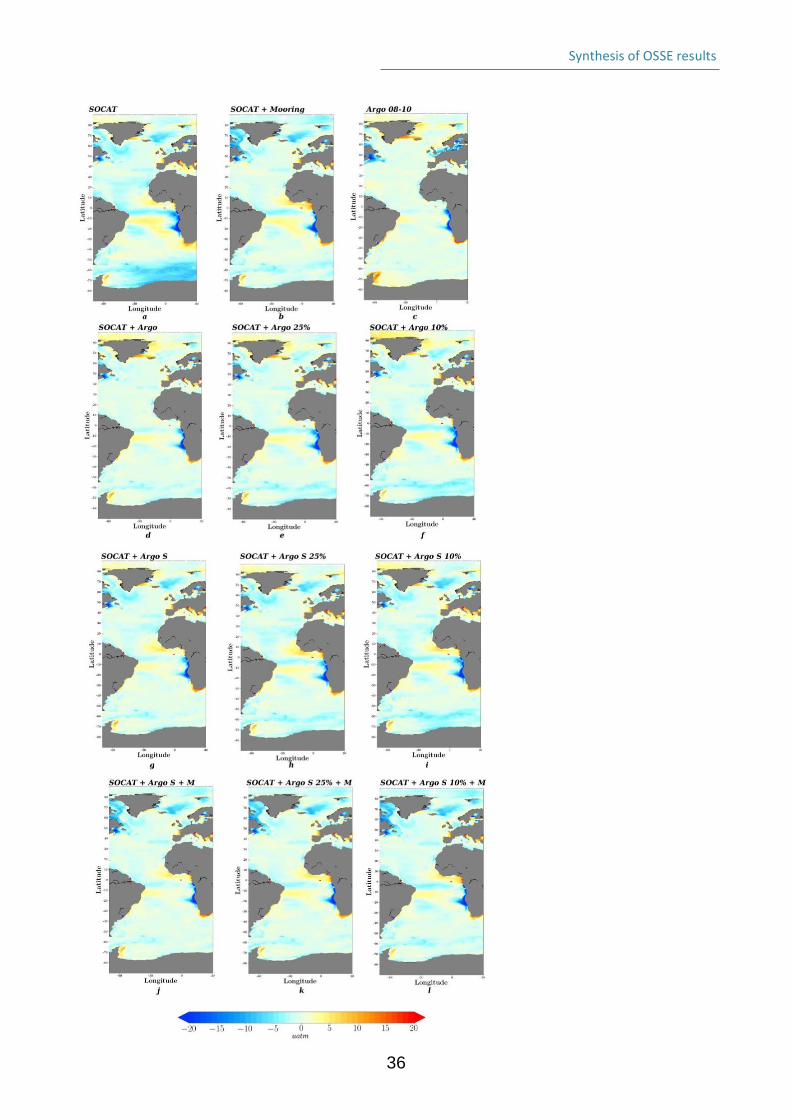
Synthesis of OSSE results
36
Synthesis of OSSE results
37
Figure 3.7: mean of difference between reconstructed and modeled pCO2 (NEMO-PISCES) for the period 2008-2010. Pseudo-observations used for training FFNN model constrained based on positions of: a – SOCAT individual data set for 2001-2010; b – SOCAT individual data set for 2001-2010 and data at all available mooring data from OceanSITES for the period 2008-2010; c – only Argo data from simulated distribution (Mercator Ocean) for 2008-2010; d – SOCAT individual data set for 2001-2010 and Argo data from simulated distribution for 2008-2010; e – SOCAT individual data set for 2001-2010 and 25% of Argo data from simulated distribution for 2008-2010; f – SOCAT individual data set for 2001-2010 and 10% of Argo data from simulated distribution for 2008-2010; g – SOCAT individual data set for 2001-2010 and Argo data in the South Hemisphere from simulated distribution for 2008-2010; h - SOCAT individual data set for 2001-2010 and 25% of all Argo data from simulated distribution added only in the South Hemisphere for 2008-2010; i - SOCAT individual data set for 2001-2010 and 10% of all Argo data from simulated distribution added only in the South Hemisphere for 2008-2010; j - SOCAT individual data set for 2001-2010, mooring data and Argo data in the South Hemisphere from simulated distribution; l - SOCAT individual data set for 2001-2010, mooring data and 25% of all Argo data from simulated distribution added only in the South Hemisphere for 2008-2010; l - SOCAT individual data set for 2001-2010, mooring data and 10% of all Argo data from simulated distribution added only in the South Hemisphere for 2008-2010.
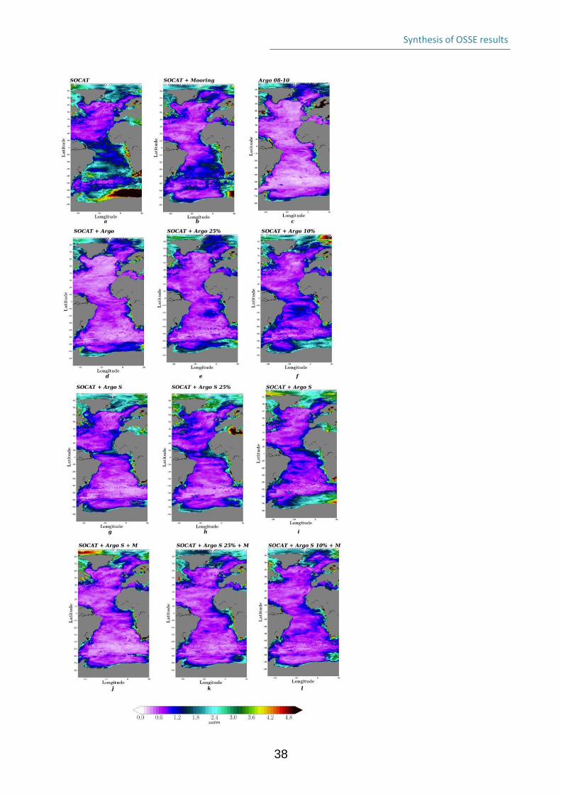
Synthesis of OSSE results
38
Synthesis of OSSE results
39
Figure 3.8: standard deviation of difference between reconstructed and modeled pCO2 (NEMO_PISCES). Pseudo-observations used for training FFNN model constrained based on positions of: a – SOCAT individual data set for 2001-2010; b – SOCAT individual data set for 2001-2010 and data at all available mooring data from OceanSITES for the period 2008-2010; c – only Argo data from simulated distribution (Mercator Ocean) for 2008-2010; d – SOCAT individual data set for 2001-2010 and Argo data from simulated distribution for 2008-2010; e – SOCAT individual data set for 2001-2010 and 25% of Argo data from simulated distribution for 2008-2010; f – SOCAT individual data set for 2001-2010 and 10% of Argo data from simulated distribution for 2008-2010; g – SOCAT individual data set for 2001-2010 and Argo data in the South Hemisphere from simulated distribution for 2008-2010; h - SOCAT individual data set for 2001-2010 and 25% of all Argo data from simulated distribution added only in the South Hemisphere for 2008-2010; i - SOCAT individual data set for 2001-2010 and 10% of all Argo data from simulated distribution added only in the South Hemisphere for 2008-2010; j - SOCAT individual data set for 2001-2010, mooring data and Argo data in the South Hemisphere from simulated distribution; l - SOCAT individual data set for 2001-2010, mooring data and 25% of all Argo data from simulated distribution added only in the South Hemisphere for 2008-2010; l - SOCAT individual data set for 2001-2010, mooring data and 10% of all Argo data from simulated distribution added only in the South Hemisphere for 2008-2010.
3.5.4. Conclusions from statistical modelling approach The aim of the work was to identify an optimal observational network of pCO2 over the Atlantic Ocean. The analysis was based on results obtained with a Feed-Forward Neural Network model trained on the SOCAT database. The SOCAT database has sparse coverage in the Southern Hemisphere. The approach consisted in adding the position of mooring data and Argo trajectories in the Atlantic Ocean to find an optimal distribution and combination of data to reconstruct pCO2 with good accuracy. A series of experiments were performed using output from the NEMO (OPA_LIM)-PISCES model. The model was sub-sampled at co-localized sites of observing systems for all predictors (SSS, SST, SSH etc.) used in the FFNN and targets (pCO2) to create pseudo-observations. Main results and recommendations are: (1) The tests highlighted the need for data in the South Atlantic Ocean. Additional data form Argo profilers in that region significantly improved pCO2 output. (2) The combination of ship data and other in-situ measurements combined in the SOCAT data base, augmented in the Southern hemisphere by a BGC ARGO density corresponding to 25% of the ARGO profiler density plus existing moorings provided a satisfying statistical result: good accuracy (comparable almost every within in the basin with the test when only Argo distribution is used (“benchmark”)) and it could probably be implemented at the least cost. (3) The network could be further improved by instrumenting Baffin Bay, the Labrador Sea, the Norwegian Sea, as well as regions along the coast of Africa (10ºN to 20ºS) with moorings or additional BGC ARGO floats. Perspective: The inclusion of errors from in-situ measurements will be an important next step of this work. It will concern the errors for predictor values (SSS, SST, SSH, etc.) that are measured directly, as well as those associated with the indirect estimation of pCO2 from pH (BGC-ARGO) and alkalinity (empirical relationship as a function of salinity).
Synthesis of OSSE results
40
4. Climate Change and Variability A range of studies has been carried out to assess the priorities for the current and future ocean observing system in the context of climate detection, monitoring and prediction. This work focuses primarily on ocean temperature change, both in terms of ocean heat content change (OHC) and also the northward heat transport in the North Atlantic, which is a key factor in the relatively mild climate of Western Europe. Global OHC change is our primary means of estimating the magnitude of Earth’s energy imbalance, and therefore a key metric for monitoring anthropogenic climate change. Variability in OHC can give rise to predictability of the ocean and climate on seasonal-to-decadal timescales. The work presented here is organised under a series of five questions:
1. How well can the historical and current in-situ observing system constrain the spatial variability and long-term change in ocean heat content?
2. How well can the historical and current in-situ observing system constrain long-term trends in deep ocean heat content (below 2000m)?
3. Where do we need deep ocean observations to track future changes in Earth’s energy imbalance from ocean heat content?
4. What sampling characteristics are needed from future observations in the deep ocean to constrain temperature and salinity changes?
5. What observations are needed to monitor future changes in the North Atlantic Ocean Heat Transport.
Key Findings:
● Analysis of both the 20th Century and future climate model projections suggest that Argo-like sampling of the upper 2000m is insufficient to accurately monitor ongoing climate change.
● The Atlantic Ocean and Southern Oceans are key areas for observations to constrain both long-term OHC trends and shorter-term variability for the 2000 - 4000m ocean. These basins should therefore be prioritized when deploying new deep observations to complement the existing Argo array.
● Assessment of temperature trends over the full ocean depth has historically relied on sparse ship-based hydrographic sections which have substantial biases. More frequent (both spatially and temporally) observations in the deep and abyssal Southern Ocean and Atlantic should be prioritized in order to better constrain these trends
● There is a clear improvement in our ability to capture the spatial patterns of OHC change in the upper 2000m (important for the initialisation of seasonal-to-decadal predictions) following the introduction of the Argo array of profiling floats.
● Development of future deep ocean observations (and analyses) should consider the spatial variations in de-correlation length scales in the ocean interior.
● Mapping methods that use neutral density coordinates (rather than z-coordinates) should make better use of the available observations due to the longer de-correlation length scales.
● A grand ensemble (GE, 100 members) of climate model simulations is able to capture the trend and variability in the observed meridional heat transport from overturning circulation at 26N.
● Climate model simulations suggest that there will be substantial changes in the North Atlantic heat transport and its variability under future climate change (mostly associated with changes in the Atlantic Meridional Overturning Circulation).
● In the coming decades, the robust decrease in the North Atlantic Ocean heat transport over the lower latitudes is associated in the models with a robust increase in the heat transport over the higher latitudes. Therefore, our study suggests the need for an observational network at 60°N, where we find the highest increase, in combination with the observational network at 26N, to detect the robust fingerprint of the global warming on the North Atlantic heat transport.
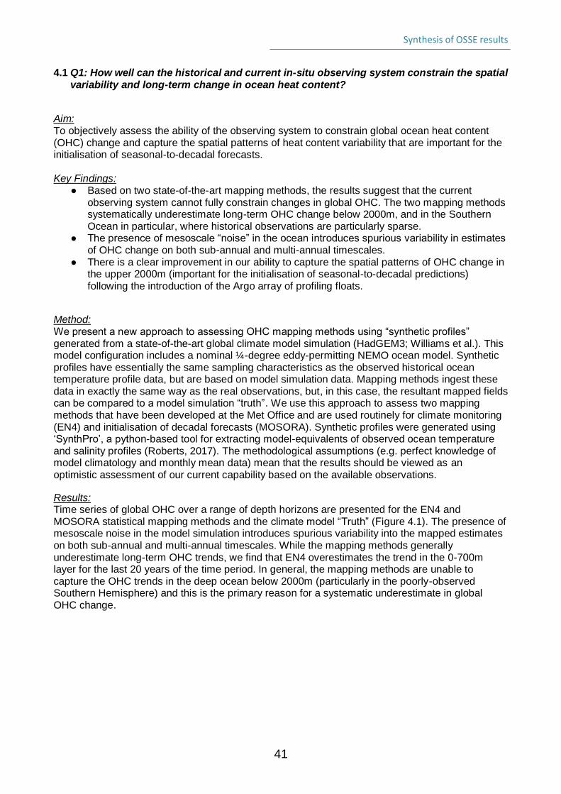
Synthesis of OSSE results
41
4.1 Q1: How well can the historical and current in-situ observing system constrain the spatial variability and long-term change in ocean heat content?
Aim: To objectively assess the ability of the observing system to constrain global ocean heat content (OHC) change and capture the spatial patterns of heat content variability that are important for the initialisation of seasonal-to-decadal forecasts. Key Findings:
● Based on two state-of-the-art mapping methods, the results suggest that the current observing system cannot fully constrain changes in global OHC. The two mapping methods systematically underestimate long-term OHC change below 2000m, and in the Southern Ocean in particular, where historical observations are particularly sparse.
● The presence of mesoscale “noise” in the ocean introduces spurious variability in estimates of OHC change on both sub-annual and multi-annual timescales.
● There is a clear improvement in our ability to capture the spatial patterns of OHC change in the upper 2000m (important for the initialisation of seasonal-to-decadal predictions) following the introduction of the Argo array of profiling floats.
Method: We present a new approach to assessing OHC mapping methods using “synthetic profiles” generated from a state-of-the-art global climate model simulation (HadGEM3; Williams et al.). This model configuration includes a nominal ¼-degree eddy-permitting NEMO ocean model. Synthetic profiles have essentially the same sampling characteristics as the observed historical ocean temperature profile data, but are based on model simulation data. Mapping methods ingest these data in exactly the same way as the real observations, but, in this case, the resultant mapped fields can be compared to a model simulation “truth”. We use this approach to assess two mapping methods that have been developed at the Met Office and are used routinely for climate monitoring (EN4) and initialisation of decadal forecasts (MOSORA). Synthetic profiles were generated using ‘SynthPro’, a python-based tool for extracting model-equivalents of observed ocean temperature and salinity profiles (Roberts, 2017). The methodological assumptions (e.g. perfect knowledge of model climatology and monthly mean data) mean that the results should be viewed as an optimistic assessment of our current capability based on the available observations.
Results: Time series of global OHC over a range of depth horizons are presented for the EN4 and MOSORA statistical mapping methods and the climate model “Truth” (Figure 4.1). The presence of mesoscale noise in the model simulation introduces spurious variability into the mapped estimates on both sub-annual and multi-annual timescales. While the mapping methods generally underestimate long-term OHC trends, we find that EN4 overestimates the trend in the 0-700m layer for the last 20 years of the time period. In general, the mapping methods are unable to capture the OHC trends in the deep ocean below 2000m (particularly in the poorly-observed Southern Hemisphere) and this is the primary reason for a systematic underestimate in global OHC change.
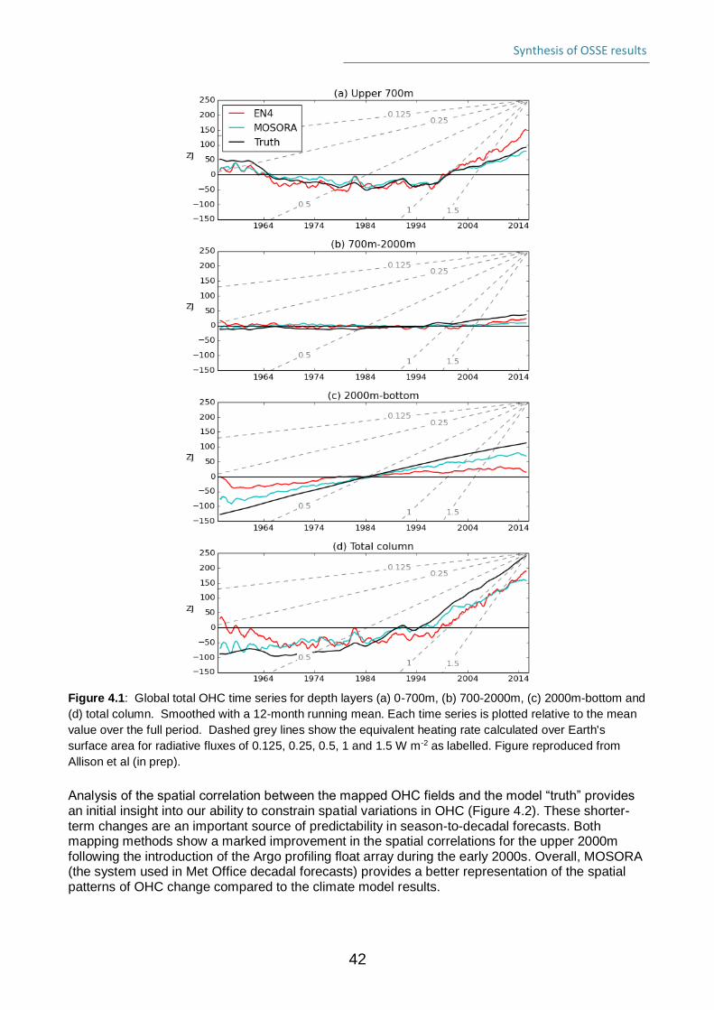
Synthesis of OSSE results
42
Figure 4.1: Global total OHC time series for depth layers (a) 0-700m, (b) 700-2000m, (c) 2000m-bottom and
(d) total column. Smoothed with a 12-month running mean. Each time series is plotted relative to the mean
value over the full period. Dashed grey lines show the equivalent heating rate calculated over Earth's
surface area for radiative fluxes of 0.125, 0.25, 0.5, 1 and 1.5 W m-2 as labelled. Figure reproduced from
Allison et al (in prep).
Analysis of the spatial correlation between the mapped OHC fields and the model “truth” provides an initial insight into our ability to constrain spatial variations in OHC (Figure 4.2). These shorter-term changes are an important source of predictability in season-to-decadal forecasts. Both mapping methods show a marked improvement in the spatial correlations for the upper 2000m following the introduction of the Argo profiling float array during the early 2000s. Overall, MOSORA (the system used in Met Office decadal forecasts) provides a better representation of the spatial patterns of OHC change compared to the climate model results.
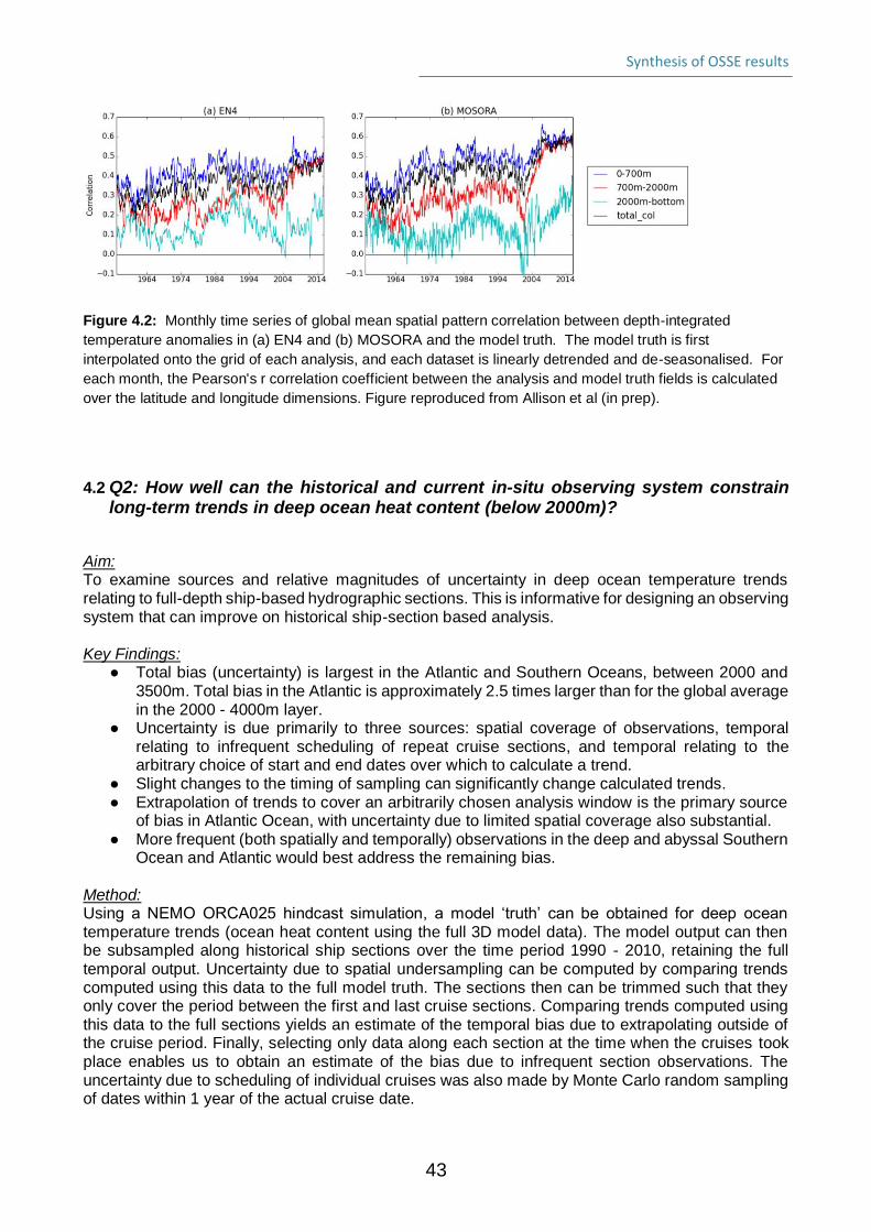
Synthesis of OSSE results
43
Figure 4.2: Monthly time series of global mean spatial pattern correlation between depth-integrated
temperature anomalies in (a) EN4 and (b) MOSORA and the model truth. The model truth is first
interpolated onto the grid of each analysis, and each dataset is linearly detrended and de-seasonalised. For
each month, the Pearson's r correlation coefficient between the analysis and model truth fields is calculated
over the latitude and longitude dimensions. Figure reproduced from Allison et al (in prep).
4.2 Q2: How well can the historical and current in-situ observing system constrain long-term trends in deep ocean heat content (below 2000m)?
Aim: To examine sources and relative magnitudes of uncertainty in deep ocean temperature trends relating to full-depth ship-based hydrographic sections. This is informative for designing an observing system that can improve on historical ship-section based analysis. Key Findings:
● Total bias (uncertainty) is largest in the Atlantic and Southern Oceans, between 2000 and 3500m. Total bias in the Atlantic is approximately 2.5 times larger than for the global average in the 2000 - 4000m layer.
● Uncertainty is due primarily to three sources: spatial coverage of observations, temporal relating to infrequent scheduling of repeat cruise sections, and temporal relating to the arbitrary choice of start and end dates over which to calculate a trend.
● Slight changes to the timing of sampling can significantly change calculated trends. ● Extrapolation of trends to cover an arbitrarily chosen analysis window is the primary source
of bias in Atlantic Ocean, with uncertainty due to limited spatial coverage also substantial. ● More frequent (both spatially and temporally) observations in the deep and abyssal Southern
Ocean and Atlantic would best address the remaining bias. Method: Using a NEMO ORCA025 hindcast simulation, a model ‘truth’ can be obtained for deep ocean temperature trends (ocean heat content using the full 3D model data). The model output can then be subsampled along historical ship sections over the time period 1990 - 2010, retaining the full temporal output. Uncertainty due to spatial undersampling can be computed by comparing trends computed using this data to the full model truth. The sections then can be trimmed such that they only cover the period between the first and last cruise sections. Comparing trends computed using this data to the full sections yields an estimate of the temporal bias due to extrapolating outside of the cruise period. Finally, selecting only data along each section at the time when the cruises took place enables us to obtain an estimate of the bias due to infrequent section observations. The uncertainty due to scheduling of individual cruises was also made by Monte Carlo random sampling of dates within 1 year of the actual cruise date.
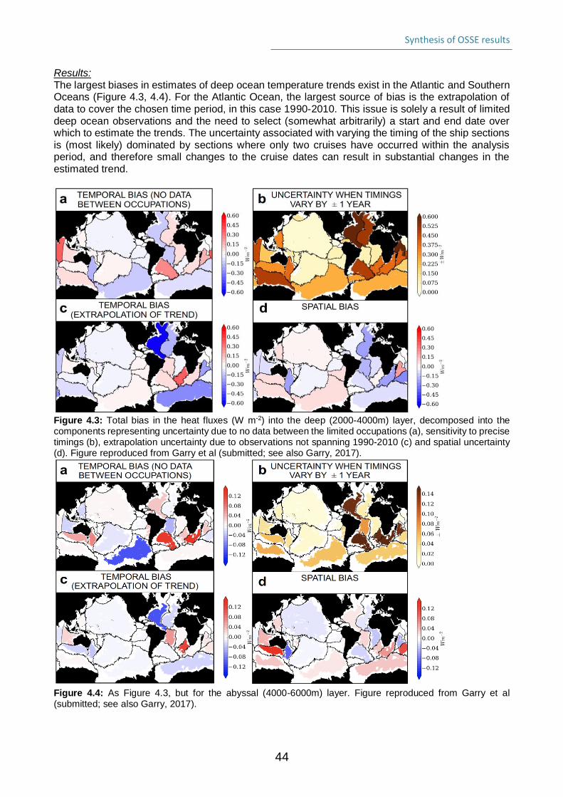
Synthesis of OSSE results
44
Results: The largest biases in estimates of deep ocean temperature trends exist in the Atlantic and Southern Oceans (Figure 4.3, 4.4). For the Atlantic Ocean, the largest source of bias is the extrapolation of data to cover the chosen time period, in this case 1990-2010. This issue is solely a result of limited deep ocean observations and the need to select (somewhat arbitrarily) a start and end date over which to estimate the trends. The uncertainty associated with varying the timing of the ship sections is (most likely) dominated by sections where only two cruises have occurred within the analysis period, and therefore small changes to the cruise dates can result in substantial changes in the estimated trend.
Figure 4.3: Total bias in the heat fluxes (W m-2) into the deep (2000-4000m) layer, decomposed into the components representing uncertainty due to no data between the limited occupations (a), sensitivity to precise timings (b), extrapolation uncertainty due to observations not spanning 1990-2010 (c) and spatial uncertainty (d). Figure reproduced from Garry et al (submitted; see also Garry, 2017).
Figure 4.4: As Figure 4.3, but for the abyssal (4000-6000m) layer. Figure reproduced from Garry et al (submitted; see also Garry, 2017).
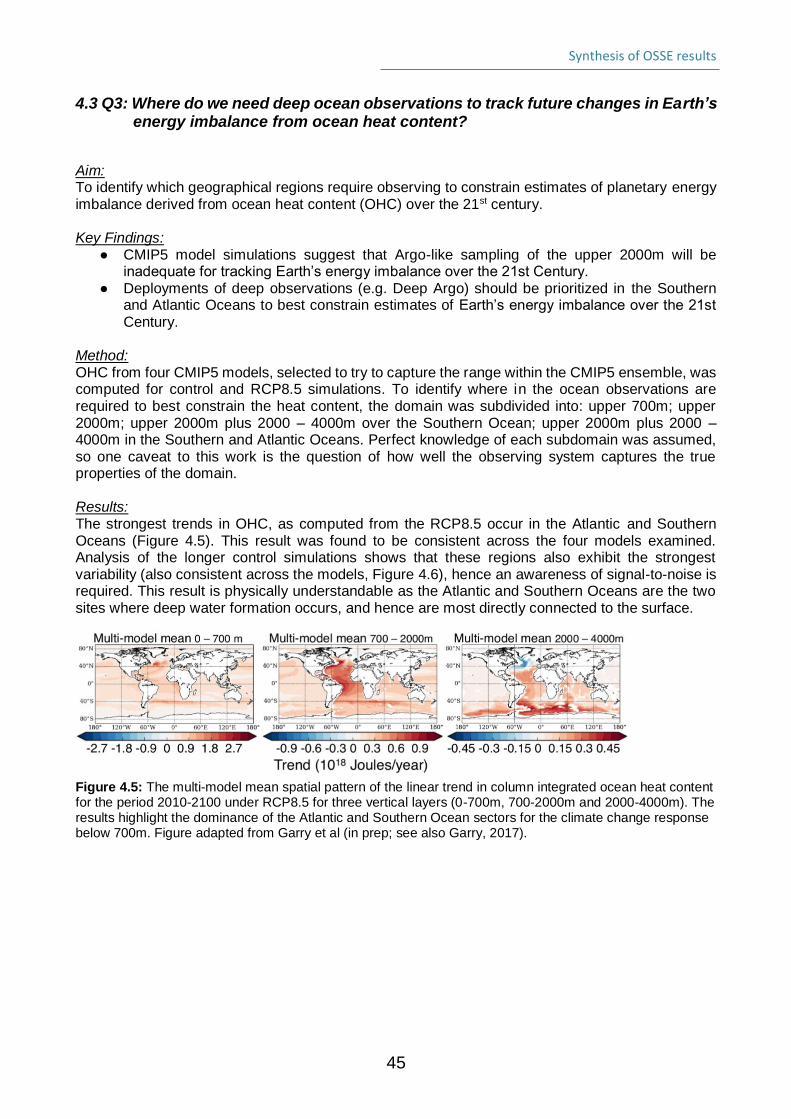
Synthesis of OSSE results
45
4.3 Q3: Where do we need deep ocean observations to track future changes in Earth’s energy imbalance from ocean heat content?
Aim: To identify which geographical regions require observing to constrain estimates of planetary energy imbalance derived from ocean heat content (OHC) over the 21st century. Key Findings:
● CMIP5 model simulations suggest that Argo-like sampling of the upper 2000m will be inadequate for tracking Earth’s energy imbalance over the 21st Century.
● Deployments of deep observations (e.g. Deep Argo) should be prioritized in the Southern and Atlantic Oceans to best constrain estimates of Earth’s energy imbalance over the 21st Century.
Method: OHC from four CMIP5 models, selected to try to capture the range within the CMIP5 ensemble, was computed for control and RCP8.5 simulations. To identify where in the ocean observations are required to best constrain the heat content, the domain was subdivided into: upper 700m; upper 2000m; upper 2000m plus 2000 – 4000m over the Southern Ocean; upper 2000m plus 2000 – 4000m in the Southern and Atlantic Oceans. Perfect knowledge of each subdomain was assumed, so one caveat to this work is the question of how well the observing system captures the true properties of the domain. Results: The strongest trends in OHC, as computed from the RCP8.5 occur in the Atlantic and Southern Oceans (Figure 4.5). This result was found to be consistent across the four models examined. Analysis of the longer control simulations shows that these regions also exhibit the strongest variability (also consistent across the models, Figure 4.6), hence an awareness of signal-to-noise is required. This result is physically understandable as the Atlantic and Southern Oceans are the two sites where deep water formation occurs, and hence are most directly connected to the surface.
Figure 4.5: The multi-model mean spatial pattern of the linear trend in column integrated ocean heat content for the period 2010-2100 under RCP8.5 for three vertical layers (0-700m, 700-2000m and 2000-4000m). The results highlight the dominance of the Atlantic and Southern Ocean sectors for the climate change response below 700m. Figure adapted from Garry et al (in prep; see also Garry, 2017).
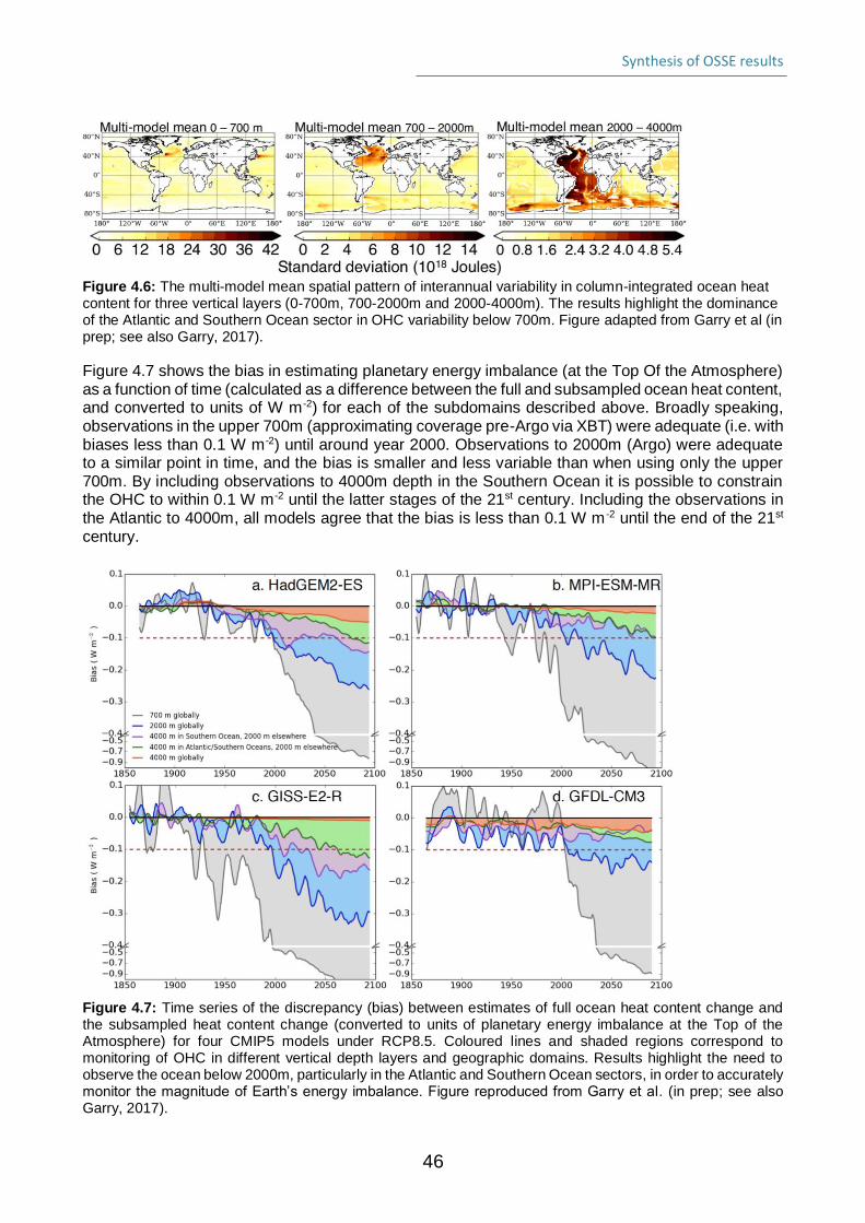
Synthesis of OSSE results
46
Figure 4.6: The multi-model mean spatial pattern of interannual variability in column-integrated ocean heat content for three vertical layers (0-700m, 700-2000m and 2000-4000m). The results highlight the dominance of the Atlantic and Southern Ocean sector in OHC variability below 700m. Figure adapted from Garry et al (in prep; see also Garry, 2017).
Figure 4.7 shows the bias in estimating planetary energy imbalance (at the Top Of the Atmosphere) as a function of time (calculated as a difference between the full and subsampled ocean heat content, and converted to units of W m-2) for each of the subdomains described above. Broadly speaking, observations in the upper 700m (approximating coverage pre-Argo via XBT) were adequate (i.e. with biases less than 0.1 W m-2) until around year 2000. Observations to 2000m (Argo) were adequate to a similar point in time, and the bias is smaller and less variable than when using only the upper 700m. By including observations to 4000m depth in the Southern Ocean it is possible to constrain the OHC to within 0.1 W m-2 until the latter stages of the 21st century. Including the observations in the Atlantic to 4000m, all models agree that the bias is less than 0.1 W m -2 until the end of the 21st century.
Figure 4.7: Time series of the discrepancy (bias) between estimates of full ocean heat content change and the subsampled heat content change (converted to units of planetary energy imbalance at the Top of the Atmosphere) for four CMIP5 models under RCP8.5. Coloured lines and shaded regions correspond to monitoring of OHC in different vertical depth layers and geographic domains. Results highlight the need to observe the ocean below 2000m, particularly in the Atlantic and Southern Ocean sectors, in order to accurately monitor the magnitude of Earth’s energy imbalance. Figure reproduced from Garry et al. (in prep; see also Garry, 2017).
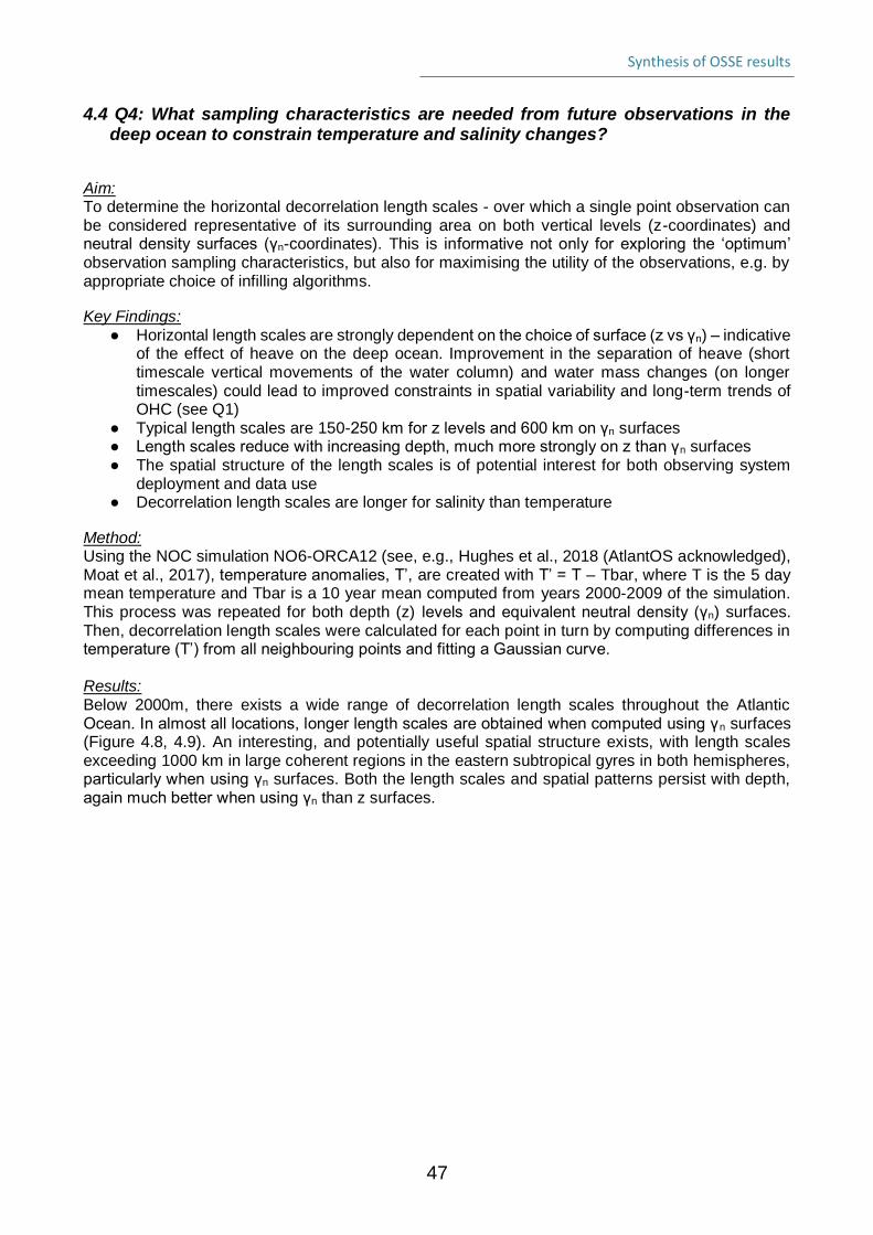
Synthesis of OSSE results
47
4.4 Q4: What sampling characteristics are needed from future observations in the deep ocean to constrain temperature and salinity changes?
Aim: To determine the horizontal decorrelation length scales - over which a single point observation can be considered representative of its surrounding area on both vertical levels (z-coordinates) and neutral density surfaces (γn-coordinates). This is informative not only for exploring the ‘optimum’ observation sampling characteristics, but also for maximising the utility of the observations, e.g. by appropriate choice of infilling algorithms.
Key Findings: ● Horizontal length scales are strongly dependent on the choice of surface (z vs γn) – indicative
of the effect of heave on the deep ocean. Improvement in the separation of heave (short timescale vertical movements of the water column) and water mass changes (on longer timescales) could lead to improved constraints in spatial variability and long-term trends of OHC (see Q1)
● Typical length scales are 150-250 km for z levels and 600 km on γn surfaces ● Length scales reduce with increasing depth, much more strongly on z than γn surfaces ● The spatial structure of the length scales is of potential interest for both observing system
deployment and data use ● Decorrelation length scales are longer for salinity than temperature
Method: Using the NOC simulation NO6-ORCA12 (see, e.g., Hughes et al., 2018 (AtlantOS acknowledged), Moat et al., 2017), temperature anomalies, T’, are created with T’ = T – Tbar, where T is the 5 day mean temperature and Tbar is a 10 year mean computed from years 2000-2009 of the simulation. This process was repeated for both depth (z) levels and equivalent neutral density (γn) surfaces. Then, decorrelation length scales were calculated for each point in turn by computing differences in temperature (T’) from all neighbouring points and fitting a Gaussian curve. Results: Below 2000m, there exists a wide range of decorrelation length scales throughout the Atlantic Ocean. In almost all locations, longer length scales are obtained when computed using γn surfaces (Figure 4.8, 4.9). An interesting, and potentially useful spatial structure exists, with length scales exceeding 1000 km in large coherent regions in the eastern subtropical gyres in both hemispheres, particularly when using γn surfaces. Both the length scales and spatial patterns persist with depth, again much better when using γn than z surfaces.
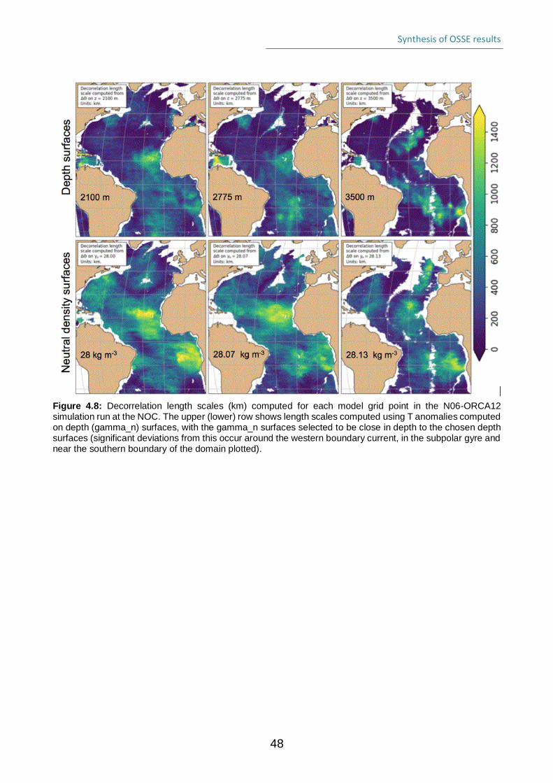
Synthesis of OSSE results
48
Figure 4.8: Decorrelation length scales (km) computed for each model grid point in the N06-ORCA12 simulation run at the NOC. The upper (lower) row shows length scales computed using T anomalies computed on depth (gamma_n) surfaces, with the gamma_n surfaces selected to be close in depth to the chosen depth surfaces (significant deviations from this occur around the western boundary current, in the subpolar gyre and near the southern boundary of the domain plotted).
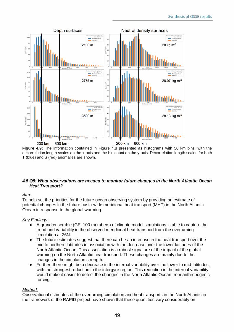
Synthesis of OSSE results
49
Figure 4.9: The information contained in Figure 4.8 presented as histograms with 50 km bins, with the decorrelation length scales on the x-axis and the bin count on the y-axis. Decorrelation length scales for both T (blue) and S (red) anomalies are shown.
4.5 Q5: What observations are needed to monitor future changes in the North Atlantic Ocean Heat Transport?
Aim: To help set the priorities for the future ocean observing system by providing an estimate of potential changes in the future basin-wide meridional heat transport (MHT) in the North Atlantic Ocean in response to the global warming. Key Findings:
● A grand ensemble (GE, 100 members) of climate model simulations is able to capture the trend and variability in the observed meridional heat transport from the overturning circulation at 26N.
● The future estimates suggest that there can be an increase in the heat transport over the mid to northern latitudes in association with the decrease over the lower latitudes of the North Atlantic Ocean. This association is a robust signature of the impact of the global warming on the North Atlantic heat transport. These changes are mainly due to the changes in the circulation strength.
● Further, there might be a decrease in the internal variability over the lower to mid-latitudes, with the strongest reduction in the intergyre region. This reduction in the internal variability would make it easier to detect the changes in the North Atlantic Ocean from anthropogenic forcing.
Method: Observational estimates of the overturning circulation and heat transports in the North Atlantic in the framework of the RAPID project have shown that these quantities vary considerably on
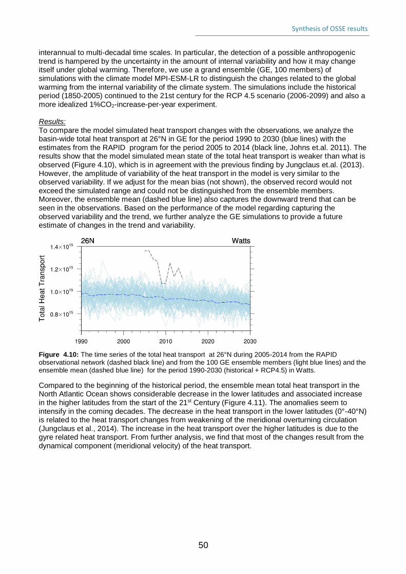
Synthesis of OSSE results
50
interannual to multi-decadal time scales. In particular, the detection of a possible anthropogenic trend is hampered by the uncertainty in the amount of internal variability and how it may change itself under global warming. Therefore, we use a grand ensemble (GE, 100 members) of simulations with the climate model MPI-ESM-LR to distinguish the changes related to the global warming from the internal variability of the climate system. The simulations include the historical period (1850-2005) continued to the 21st century for the RCP 4.5 scenario (2006-2099) and also a more idealized 1%CO2-increase-per-year experiment. Results: To compare the model simulated heat transport changes with the observations, we analyze the basin-wide total heat transport at 26°N in GE for the period 1990 to 2030 (blue lines) with the estimates from the RAPID program for the period 2005 to 2014 (black line, Johns et.al. 2011). The results show that the model simulated mean state of the total heat transport is weaker than what is observed (Figure 4.10), which is in agreement with the previous finding by Jungclaus et.al. (2013). However, the amplitude of variability of the heat transport in the model is very similar to the observed variability. If we adjust for the mean bias (not shown), the observed record would not exceed the simulated range and could not be distinguished from the ensemble members. Moreover, the ensemble mean (dashed blue line) also captures the downward trend that can be seen in the observations. Based on the performance of the model regarding capturing the observed variability and the trend, we further analyze the GE simulations to provide a future estimate of changes in the trend and variability.
Figure 4.10: The time series of the total heat transport at 26°N during 2005-2014 from the RAPID observational network (dashed black line) and from the 100 GE ensemble members (light blue lines) and the ensemble mean (dashed blue line) for the period 1990-2030 (historical + RCP4.5) in Watts.
Compared to the beginning of the historical period, the ensemble mean total heat transport in the North Atlantic Ocean shows considerable decrease in the lower latitudes and associated increase in the higher latitudes from the start of the 21st Century (Figure 4.11). The anomalies seem to intensify in the coming decades. The decrease in the heat transport in the lower latitudes (0°-40°N) is related to the heat transport changes from weakening of the meridional overturning circulation (Jungclaus et al., 2014). The increase in the heat transport over the higher latitudes is due to the gyre related heat transport. From further analysis, we find that most of the changes result from the dynamical component (meridional velocity) of the heat transport.
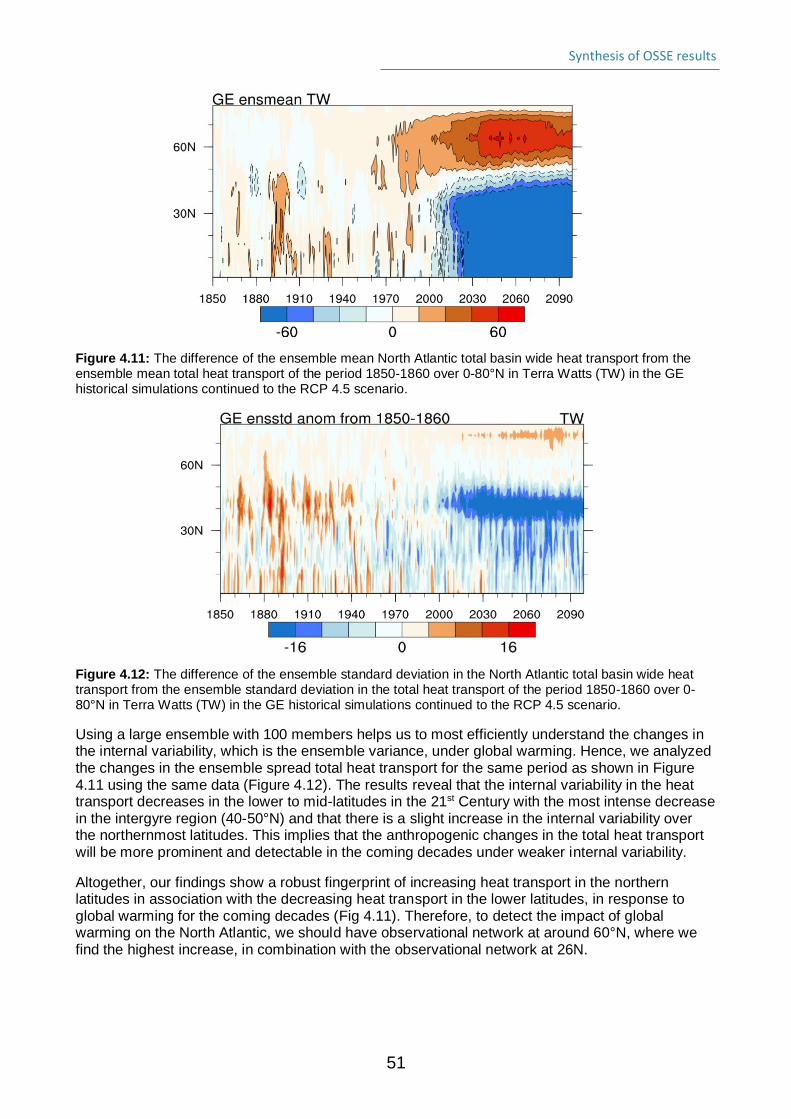
Synthesis of OSSE results
51
Figure 4.11: The difference of the ensemble mean North Atlantic total basin wide heat transport from the ensemble mean total heat transport of the period 1850-1860 over 0-80°N in Terra Watts (TW) in the GE historical simulations continued to the RCP 4.5 scenario.
Figure 4.12: The difference of the ensemble standard deviation in the North Atlantic total basin wide heat transport from the ensemble standard deviation in the total heat transport of the period 1850-1860 over 0-80°N in Terra Watts (TW) in the GE historical simulations continued to the RCP 4.5 scenario.
Using a large ensemble with 100 members helps us to most efficiently understand the changes in the internal variability, which is the ensemble variance, under global warming. Hence, we analyzed the changes in the ensemble spread total heat transport for the same period as shown in Figure 4.11 using the same data (Figure 4.12). The results reveal that the internal variability in the heat transport decreases in the lower to mid-latitudes in the 21st Century with the most intense decrease in the intergyre region (40-50°N) and that there is a slight increase in the internal variability over the northernmost latitudes. This implies that the anthropogenic changes in the total heat transport will be more prominent and detectable in the coming decades under weaker internal variability.
Altogether, our findings show a robust fingerprint of increasing heat transport in the northern latitudes in association with the decreasing heat transport in the lower latitudes, in response to global warming for the coming decades (Fig 4.11). Therefore, to detect the impact of global warming on the North Atlantic, we should have observational network at around 60°N, where we find the highest increase, in combination with the observational network at 26N.
Synthesis of OSSE results
52
5 Publications and Code associated with this deliverable:
AtlantOS acknowledged publications:
● Hughes, C. W., Williams, J., Blaker, A., Coward, A., & Stepanov, V. (2018). A window on the deep ocean: The special value of ocean bottom pressure for monitoring the large-scale, deep-ocean circulation. Prog. Oceanogr., 161, 19-46. doi:10.1016/j.pocean.2018.01.011
● Garry, F. K., McDonagh, E., Blaker, A. T., Roberts, C. D., Desbruyères, D. G., Frajka-Williams, E., King, B. A., 2018: JGR Oceans, submitted.
● Hedemann, C., Mauritsen, T., Jungclaus, J., and Marotzke, J., 2017: The subtle origins of surface-warming hiatuses. Nature Climate Change, 7, 336-339 , doi:10.1038/nclimate3274.
● Gasparin, F. et al., 2018, A large-scale view of oceanic variability from 2007 to 2015 in the global high resolution monitoring and forecasting system at Mercator Océan, Journal of Marine Systems, https://doi.org/10.1016/j.jmarsys.2018.06.015
● Mirouze I and Storto A. 2018. Generating atmospheric forcing perturbations for an ocean data assimilation ensemble. Submitted to Dynamics of Atmospheres and Oceans.
AtlantOS publications in preparation:
● Allison, L.C., C.D. Roberts, M.D. Palmer, R. Killick, L. Hermanson, N.A. Rayner and D.M. Smith, Towards quantifying uncertainty in ocean heat content changes using synthetic profiles, in preparation.
● Garry, F. K., Roberts, C. D., Frajka-Williams, E., McDonagh, E., Blaker, A. T., and King, B. A., Where do we need deep ocean observations to estimate planetary energy imbalance from ocean heat content?, in preparation.
• Ghosh, R., Jungclaus, J., Lohmann, K., Matei, D., Disentangling the effect of the global warming from the internal variability in the North Atlantic heat transport, in preparation
• Gasparin, F., S. Guinehut, C. Mao, I. Mirouze, E. Remy, R. King, M. Hamon, R. Reid, S. Massina, M. Martin, P.Y Le Traon, 2018: Requirements for an integrated Atlantic Ocean Observing System from internationally-coordinated Observing System Simulation Experiments, In preparation.
• Gasparin F., E. Remy, M. Hamon, P.Y Le Traon, 2018: Assessment of the Deep Argo Array Inferred from Observing System Simulation Experiments, In preparation.
• Ford, D. et al. (Description of Met Office biogeochemical OSSEs) (in preparation)
• Germinaud, C. et al. (Description of CNRS/IGE biogeochemical OSSEs) (in preparation)
• Sommer, A., M. Gehlen, M. Vrac, C. Mejia A novel neural network model for the operational reconstruction of surface ocean pCO2. To be submitted to Geoscientific Model Development (September 2018)
• Sommer, A., M. Gehlen, M. Vrac, C. Mejia, Towards an integrated multi-platform observing system for surface ocean carbon system variables at the scale of the Atlantic Ocean (in preparation).
AtlantOS publication planned:
• (Mercator-Océan) – Paper describing Mercator-Océan results for physics OSSEs
• (MetOffice) – Paper describing Met Office Physics OSSE results
• (CLS) – Paper describing CLS physics OSSE results
• (CMCC) - Paper describing CMCC physics OSSE results
• Ford, D., C. Germinaud et al. – Synthesis paper on Met Office and CNRS/IGE biogeochemical results
Computer code:
• Python code to extract synthetic profiles from arbitrary ocean model data has been made available by Roberts (2017): https://github.com/cdr30/SynthPro
Synthesis of OSSE results
53
References Allison, L.C., C.D. Roberts, M.D. Palmer, R. Killick, L. Hermanson, N.A. Rayner and D.M. Smith, Towards quantifying uncertainty in ocean heat content changes using synthetic profiles, in preparation. Anderson, J. L. (1996). A method for producing and evaluating probabilistic forecasts from ensemble model integrations. Journal of Climate, 9 (7), 1518–1530. Anderson, L. A., Robinson, A. R., & Lozano, C. J. (2000). Physical and biological modeling in the Gulf Stream region: I. Data assimilation methodology. Deep Sea Research Part I: Oceanographic Research Papers, 47(10), 1787-1827. Bakker et al. (2016) A multi-decade record of high quality fCO₂ data in version 3 of the Surface Ocean CO₂ Atlas (SOCAT). Earth System Science Data, 8: 383-413. doi:10.5194/essd-8-383-2016 Balmaseda, M., and D. Anderson, 2009: Impact of initialization strategies and observations on seasonal forecast skill. Geophys. Res. Lett., 36. Balmaseda, M.A., F. Hernandez, A. Storto, M.D. Palmer, O. Alves, L. Shi, G.C. Smith, T. Toyoda, M. Valdivieso, B. Barnier, D. Behringer, T. Boyer, Y-S. Chang, G.A. Chepurin, N. Ferry, G. Forget, Y. Fujii, S. Good, S. Guinehut, K. Haines, Y. Ishikawa, S. Keeley, A. Köhl, T. Lee, M.J. Martin, S. Masina, S. Masuda, B. Meyssignac, K. Mogensen, L. Parent, K.A. Peterson,Y.M. Tang, Y. Yin, G. Vernieres, X. Wang, J. Waters, R. Wedd, O. Wang, Y. Xue, M. Chevallier, J-F. Lemieux, F. Dupont, T. Kuragano, M. Kamachi, T. Awaji, A. Caltabiano, K. Wilmer-Becker & F. Gaillard (2015) The Ocean Reanalyses Intercomparison Project (ORA-IP), Journal of Operational Oceanography, 8:sup1, s80-s97, DOI:10.1080/1755876X.2015.1022329 Bell, M.J., Schiller, A., Le Traon, P.Y., Smith, N.R., Dombrowsky, E., Wilmer- Becker, K., 2015. An introduction to GODAE OceanView. Taylor & Francis. Bishop, C.M. (1995). Neural Networks for Pattern Recognition. Oxford Univ. Press, Cambridge, U. K. Boss, E., et al. (2008). Observations of pigment and particle distributions in the western North Atlantic from an autonomous float and ocean color satellite. Limnology and Oceanography, 53(5part2), 2112-2122. Brankart, J.-M., G. Candille, F. Garnier, C. Calone, A. Melet, P.-A. Bouttier, P. Brasseur, and J. Verron, 2015: A generic approach to explicit simulation of uncertainty in the NEMO ocean model. Geoscientific Model Development, 8 (5), 1285–1297. Cabanes, C., Grouazel, A., von Schuckmann, K., Hamon, M., Turpin, V., Coatanoan, C., Paris, F., Guinehut, S., Boone, C., Ferry, N., de Boyer Montgut, C., Carval, T., Reverdin, G., Pouliquen, S., Le Traon, P.Y., 2013. The CORA dataset: validation and diagnostics of in-situ ocean temperature and salinity measurements. Ocean Sci. 9, 1–18. doi:10.5194/ os-9-1-2013. Candille, G., C. Côté, P. L. Houtekamer, and G. Pellerin, 2007: Verification of an ensemble pre- diction system against observations. Monthly Weather Review, 135 (7), 2688–2699. Ciavatta, S., Torres, R., Martinez-Vicente, V., Smyth, T., Dall’Olmo, G., Polimene, L., & Allen, J. I. (2014). Assimilation of remotely-sensed optical properties to improve marine biogeochemistry modelling. Progress in Oceanography, 127, 74-95. Dee, D. P., et al. (2011). The ERA‐Interim reanalysis: Configuration and performance of the data assimilation
system. Quarterly Journal of the royal meteorological society, 137(656), 553-597. FAO (2016). The State of World Fisheries and Aquaculture 2016. Contributing to food security and nutrition for all. Rome. 200 pp. Ford, D., & Barciela, R. (2017). Global marine biogeochemical reanalyses assimilating two different sets of merged ocean colour products. Remote Sensing of Environment, 203, 40-54.
Synthesis of OSSE results
54
Fujii Y, Cummings J, Xue Y, Schiller A, Lee T, Balmaseda MA, Remy E, Masuda S, Brassington G, Alves O, Cornuelle B, Martin M, Oke P, Smith G, Yang X (2015) Evaluation of the tropical Pacific observing system from the ocean data assimilation perspective. Q J R Meteorol Soc. doi: 10.1002/qj.2579 Garnier, F., J.-M. Brankart, P. Brasseur, and E. Cosme, 2016: Stochastic parameterizations of biogeochemical uncertainties in a 1/4° NEMO/PISCES model for probabilistic comparisons with ocean color data. Journal of Marine Systems, 155 (Supplement C), 59–72. Garry, F. K., McDonagh, E., Blaker, A. T., Roberts, C. D., Desbruyères, D. G., Frajka-Williams, E., King, B. A., 2018: JGR Oceans, submitted (AtlantOS acknowledged) Garry, F. K., Roberts, C. D., Frajka-Williams, E., McDonagh, E., Blaker, A. T., and King, B. A., Where do we need deep ocean observations to estimate planetary energy imbalance from ocean heat content?, in preparation. (AtlantOS acknowledged) Gasparin et al., 2018, A large-scale view of oceanic variability from 2007 to 2015 in the global high-resolution monitoring and forecasting system at Mercator Océan, In revision in Journal of Marine Systems Gehlen, M., et al. (2015). Building the capacity for forecasting marine biogeochemistry and ecosystems: recent advances and future developments. Journal of Operational Oceanography, 8(sup1), s168-s187. Good, S.A., Martin, M.J., Rayner, N.A., 2013. EN4: Quality controlled ocean temperature and salinity profiles and monthly objective analyses with uncer- tainty estimates. Journal of Geophysical Research: Oceans 118, 6704–6716. Halliwell, G. R., A. Srinivasan, V. Kourafalou, H. Yang, D. Willey, M. Le Hénaff, and R. Atlas, 2014: Rigorous evaluation of a fraternal twin ocean OSSE system for the open Gulf of Mexico. Journal of Atmospheric and Oceanic Technology, 31 (1), 105–130. Hersbach, H., 2000: Decomposition of the continuous ranked probability score for ensemble prediction systems. Weather and Forecasting, 15 (5), 559–570. Hughes, C. W., Williams, J., Blaker, A., Coward, A., & Stepanov, V. (2018). A window on the deep ocean: The special value of ocean bottom pressure for monitoring the large-scale, deep-ocean circulation. Prog. Oceanogr., 161, 19-46. doi:10.1016/j.pocean.2018.01.011 Johns, W.E., Baringer, M.O., Beal, L.M., Cunningham, S.A., Kanzow, T., Bryden, H.L., Hirschi, J.J.M., Marotzke, J., Meinen, C.S., Shaw, B. and Curry, R., 2011. Continuous, array-based estimates of Atlantic Ocean heat transport at 26.5 N. Journal of Climate, 24(10), pp.2429-244. Johnson, K., & Claustre, H. (2016). The scientific rationale, design, and implementation plan for a Biogeochemical-Argo float array. Biogeochem.-Argo Plann. Group, 58. Johnson, K. S., et al. (2017). Biogeochemical sensor performance in the SOCCOM profiling float array. Journal of Geophysical Research: Oceans. Jungclaus, J.H., N. Fischer, H. Haak, K. Lohmann, J. Marotzke, D. Matei, U. Mikolajewicz, D. Notz, and J.-S. von Storch, 2013: Characteristics of the ocean simulations in MPIOM, the ocean component of the MPI-Earth System Model. Journal of Advances in Modeling Earth Systems, 5, 1-25, doi:10.1002/jame.20023 Jungclaus, J.H., K. Lohmann, and D. Zanchettin, 2014: Enhanced 20th century heat transfer to the Arctic simulated in the context of climate variations over the last millennium. Climate of the Past, 10, 2201-2213, doi:10.5194/cp-10-2201-2014. Kobayashi, S., et al. (2015). The JRA-55 reanalysis: General specifications and basic characteristics. Journal of the Meteorological Society of Japan. Ser. II, 93(1), 5-48. Lellouche, J.M., Greiner, E., Le Galloudec, O., Garric, G., Regnier, C., Dre- villon, M., Benkiran, M., Testut, C.E., Bourdalle-Badie, R., Gasparin, F., Hernandez, O., Levier, B., Drillet, Y., Remy, E., Le Traon, P.Y.,
Synthesis of OSSE results
55
2018. Re- cent updates on the Copernicus Marine Service global ocean monitoring and forecasting real-time 1/12 high-resolution system. Ocean Sci. Discuss. 2018, 1–70. doi:10.5194/os-2018-15. Longhurst, A., 1995: Seasonal cycles of pelagic production and consumption. Progress in Oceanography, 36 (2), 77–167. Lumpkin, R., and M. Pazos, 2007: Measuring surface currents with surface velocity program drifters: The instruments, its data and some recent results. Lagrangian Analysis and Prediction of Coastal and Ocean Dynamics, A. Griffa et al., Eds., Cambridge University Press, 39–67. Madec, G., the NEMO team, 2008. Nemo ocean engine: Note du pole de modlisation, Institut Pierre-Simon Laplace (IPSL), France, No 27 ISSN No 12881619. Tech. Rep. McClain, C. R. (2009). A decade of satellite ocean color observations. Annual Review of Marine Science, 1, 19-42. McPhaden, M.J., Ando, K., Bourles, B., Freitag, H., Lumpkin, R., Masumoto, Y., Murty, V., Nobre, P., Ravichandran, M., Vialard, J., Vousden, D., Yu, W., 2010 : The global tropical moored buoy array. Proceedings of OceanObs 9. Moat, B. I., Josey, S. A., Sinha, B., Blaker, A.T., Smeed, D. A., McCarthy, G., Johns, W. E., Hirschi, J. J-M., Frajke-Williams, E., Rayner, D., Duchez, A., Coward, A. C., 2016. Major variations in subtropical North Atlantic heat transport at short (5 day) time scales and their causes, JGR-Oceans, 121 (5), 3237-3249, doi:10.1002/2016JC011660 Oke, P. R., Larnicol, G., Fujii, Y., Smith, G. C., Lea, D. J., Guinehut, S., Rémy, E., Alonso Balmaseda, M., Rykova, T., Surcel- Colan, D., Martin, M. J., Sellar, A. A., Mulet, S., and Turpin, V.: Assessing the impact of observations on ocean forecasts and re- analyses: Part 1, Global studies, J. Oper. Oceanogr., 8, s49–s62, https://doi.org/10.1080/1755876X.2015.1022067, 2015. Park, J. Y., Stock, C. A., Yang, X., Dunne, J. P., Rosati, A., John, J., & Zhang, S. (2018). Modeling global ocean biogeochemistry with physical data assimilation: A pragmatic solution to the equatorial instability. Journal of Advances in Modeling Earth Systems, 10(3), 891-906. Purkey, S.G., Johnson, G.C., 2010. Warming of Global Abyssal and Deep South- ern Ocean Waters between the 1990s and 2000s: Contributions to Global Heat and Sea Level Rise Budgets*. Journal of Climate 23, 6336–6351. Raghukumar, K., Edwards, C. A., Goebel, N. L., Broquet, G., Veneziani, M., Moore, A. M., & Zehr, J. P. (2015). Impact of assimilating physical oceanographic data on modeled ecosystem dynamics in the California Current System. Progress in Oceanography, 138, 546-558. Roberts, C. D. (2017), cdr30/SynthPro: SynthPro v1.0.0. doi:10.5281/zenodo.1036333. Rödenbeck, C., Bakker, D. C. E., Gruber, N., Iida, Y., Jacobson, A. R., Jones, S., Landschützer, P., Metzl, N., Nakaoka, S., Olsen, A., Park, G.-H., Peylin, P., Rodgers, K. B., Sasse, T. P., Schuster, U., Shutler, J. D., Valsala, V., Wanninkhof, R., and Zeng, J.: Data-based estimates of the ocean carbon sink variability – first results of the Surface Ocean pCO2 Mapping intercomparison (SOCOM), Biogeosciences, 12, 7251-7278,
https://doi.org/10.5194/bg-12-7251-2015, 2015. Roemmich, D., G. C. Johnson, S. Riser, R. Davis, J. Gilson, W. B. Owens, S. L. Garzoli, C. Schmid, and M. Ignaszewski, B., 2009 : The Argo program observing the Global Ocean with profiling floats, Oceanography, vol. 22, pp. 34–43. Roulston, M. S., and L. A. Smith, 2002: Evaluating probabilistic forecasts using information theory. Monthly Weather Review, 130 (6), 1653–1660. Rumelhart, D.E., Hinton, G.E., & Williams, R.J. (1986). Learning internal representations by backpropagating errors. Nature, 323, 533–536 Ryan, A., Regnier, C., Divakaran, P., Spindler, T., Mehra, A., Smith, G., David- son, F., Hernandez, F., Maksymczuk, J., Liu, Y., 2015. GODAE OceanView 26, Class 4 forecast verification framework: global ocean
Synthesis of OSSE results
56
inter-comparison. Jour- nal of Operational Oceanography 8, s98–s111. doi:10.1080/1755876X.2015. 1022330. Szekely, T., Gourrion, J., Pouliquen, S., Reverdin, G., 2016. CORA, Coriolis Ocean Dataset for Reanalysis. SEANOE doi:http://doi.org/10.17882/ 46219 Talagrand, O., R. Vautard, and B. Strauss, 1997: Evaluation of prob- abilistic prediction systems. Proceedings, ECMWF Workshop on Predictability, ECMWF, 1–25. [Available from ECMWF, Shinfield Park, Reading, Berkshire RG2 9AX, United Kingdom.] Titchner, H. A., and N. A. Rayner, 2014: The Met Office Hadley Centre sea ice and sea surface temperature data set, version 2: 1. Sea ice concentrations. J. Geophys. Res. Atmospheres, 119, 2864–2889. Turpin, V., Remy, E., and Le Traon, P. Y., 2015: How essential are Argo observations to constrain a global ocean data assimilation system, Ocean Sci., 12, 257–274, https://doi.org/10.5194/os-12- 257-2016, 2016. Visbeck, M., et al., 2015: More Integrated and More Sustainable Atlantic Ocean Observing System (AtlantOS). CLIVAR Exchanges, 67 (2), 18–20. von Schuckmann, K., and P.‐Y. Le Traon (2011), How well can we derive Global Ocean Indicators from Argo
data? Ocean Sci. Discuss., 8, 999–1024, doi:10.5194/osd‐8‐999‐2011.
Waters, J., Lea, D. J., Martin, M. J., Mirouze, I., Weaver, A., & While, J. (2015). Implementing a variational data assimilation system in an operational 1/4 degree global ocean model. Quarterly Journal of the Royal Meteorological Society, 141(687), 333-349. While, J., Totterdell, I., & Martin, M. (2012). Assimilation of pCO2 data into a global coupled physical‐biogeochemical ocean model. Journal of Geophysical Research: Oceans, 117(C3). Wilks, D. S., 2011: Statistical methods in the atmospheric sciences. Academic press,. Zuo, H., M. A. Balmaseda, and K. Mogensen, 2017: The new eddy-permitting ORAP5 ocean reanalysis: description, evaluation and uncertainties in climate signals. Clim. Dyn., 49, 791–811. ——, M. A. Balmaseda, K. Mogensen, and S. Tietsche, 2018: OCEAN5: the ECMWF Ocean Reanalysis System and its Real-Time analysis component. ECMWF Tech Memo, 823.

Last update: 10 October 2018
This project has received funding from the European Union’s Horizon 2020 research and innovation
programme under grant agreement no 633211.
Project AtlantOS – 633211
Deliverable number 1.5 – Appendices
Deliverable title Synthesis of OSSE results
Description Appendices A-C to Observing System Simulation Experiments (OSSEs): Report describing the robust results obtained from across the models.
Work Package number 1
Work Package title Observing System Requirements and Design Studies
Lead beneficiary Met Office
Lead authors C. Mao (Met Office), I. Mirouze (CMCC), S. Guinehut (CLS)
Contributors R. King, R. Reid, M. Martin and S. Good
Submission data Submitted alongside main report for D1.5
Due date August 2018
Comments An extension to the original deadline was requested to allow time for integration of the results from the complex OSSE intercomparison. This is the first time such an intercomparison has been undertaken.

Synthesis of OSSE results – Appendices
2
Stakeholder engagement relating to this task*
WHO are your most important stakeholders?
☐ National governmental body
☐ International organization Please give the name(s) of the stakeholder(s): World Climate Research Programme Global Ocean Observing System
WHERE is/are the company(ies) or organization(s) from?
Please name the country(ies): International
Is this deliverable a success story? If yes, why?
If not, why?
Yes, because the most coordinated set of studies to date has been successfully completed to examine the potential of different options for the future ocean observing system. Specific impacts of different observing elements have been assessed for data assimilating ocean models (analyses), and the need to future-proof the observing system to detect future climate change has been demonstrated and quantified.
Will this deliverable be used?
If yes, who will use it?
If not, why will it not be used?
Yes, the results (and resulting publications in the peer-reviewed literature) will be influential in international thinking about the shape of the future global ocean observing system. For example, the results are expected to be an important input to the once-per-decade OceanObs 2019 conference.
NOTE: This information is being collected for the following purposes:
1. To make a list of all companies/organizations with which AtlantOS partners have had contact. This is important to demonstrate the extent of industry and public-sector collaboration in the obs community. Please note that we will only publish one aggregated list of companies and not mention specific partnerships.
2. To better report success stories from the AtlantOS community on how observing delivers concrete value to society.
*For ideas about relations with stakeholders you are invited to consult D10.5 Best Practices in Stakeholder Engagement, Data Dissemination and Exploitation.
Synthesis of OSSE results – Appendices
3
APPENDIX A: OSSE results using the Met Office FOAM system
Chongyuan Mao, Robert King, Rebecca Reid, Matthew Martin and Simon Good (Met Office)
A.1 Overview
A.1.1 Introduction
This report is a contribution (Appendix A) to D1.5 on “Synthesis of OSSE results”. It presents results using the Met Office operational Forecasting Ocean Assimilation Model (FOAM) system. This high-resolution global ocean model is on extended ORCA grid at ¼◦ horizontal resolution with 75 vertical levels. The OSSEs is forced by surface fluxes from the Japanese 55-year Reanalysis (JRA55), produced by Japan Meteorological Agency (JMA, Ebita, et al., 2011; Kobayashi, et al., 2015). The system is initialized using the outputs from the last year of a long-running free run that ended in 2006. A 3D-Var NEMOVAR scheme is used to assimilate physical variables into the system (Waters, et al. 2015). No further quality control is applied to the simulated datasets as all required quality control had been applied during the production of these datasets. The OSSEs cover the 2-year period from January 2008, with the first 6 months (January - June 2008) as the spin-up period. Mercator Océan provides a Nature Run (NR, Gasparin, et al., 2017), which is considered the “true” ocean state and is also used to generate the simulated observations for experiments carried out at all participating groups (Mercator Océan, Met Office, CMCC and CLS). The mean bias and root mean square error (RMSE) of OSSE minus NR (OSSE-NR) are used to assess the impact of the system. Both Met Office OSSEs and NR are interpolated to a common ¼◦ ORCA grid with 50 vertical levels before statistical comparison.
To study the impact of the enhancement of the Atlantic Ocean observing system on the ocean state estimate using the FOAM system, as part of task 1.3.1, the Met Office has carried on the following experiments:
• Free Run: No data assimilation but provides statistical estimate of system error
• Backbone: Assimilates simulated observations from full near-future observing network ▪ Along track SLA observations from Sentinel-3A, 3B and Jason-2 ▪ Profile observations from the existing Argo array, XBTs and moorings ▪ SST observations from drifting and moored buoys, ships, 3 infrared and 1 microwave satellite ▪ Sea ice concentration observations from satellite
• WBC_Argo2X: Similar to Backbone but also assimilates additional Argo profiles in the western boundary current (WBC) regions and near the Equator
• Deep Argo: Similar to Backbone run but also assimilates additional Deep Argo profiles down to 6000 m depth, which are about one-third of all Argo floats
• Mooring: Similar to Backbone run but removes all profiles from moorings
Results for each of these experiments are summarised in the following sections. Most results in this report are from January – December 2009, unless specified otherwise. The complete and detailed description of the work is available in Section A.3.
A.1.2 Free Run
First, the simulated observations are assessed by performing a Free Run (hereafter FR) that verifies these observations during January - March 2008. Here, the observations are not assimilated but are compared to model outputs to produce observations-minus-background (O-B) statistics. The results are then compared to another FR that verifies real observations during the same period. The aim is to test if the errors were similar using real and simulated observations. For the Global Ocean, the bias and RMSE of FOAM verifying real and simulated observations are comparable, with the O-B verifying simulated observations slightly smaller than those using real observations. The mean bias is ~0.5 °C for temperature and ~0.2 psu for salinity; the temperature RMSE is ~2.0 °C and ~0.5 psu for salinity (see Section 3 for details). It is safe to conclude that the simulated observations can be used for the OSSEs.
Synthesis of OSSE results – Appendices
4
A.1.3 Backbone
The Backbone run (hereafter BB) assimilates the simulated observations from the full near-future observing network. The temperature and salinity bias and RMSE for BB-NR are largely reduced from those for FR-NR in the Atlantic. More specifically, the warm (top 100 m) and cold (100 – 500 m) biases around ±0.5 °C seen in FR-NR are reduced to <0.1 °C for most depths, except at depth 100 m where the bias is still around 0.3 °C in BB-FR. The fresh bias with magnitude >0.2 psu in FR-NR at the top 25 m is reduced to ~0.08 psu (see Section 3 for more details). The BB run is still slightly fresher than the NR at surface, potentially due to the different surfaced fluxes used in NR and Met Office OSSEs. The RMSE for both temperature and salinity are also significantly reduced in BB-NR compared to FR-NR. Therefore, the FOAM system can reproduce and provide useful information of the ocean state by assimilating observations in the full near-future observing network.
A.1.4 WBC_Argo2X
The WBC_Argo2X experiment uses the same observations as the Backbone experiment plus additional in-situ temperature and salinity Argo profiles at the Equator and in the WBC regions where their sampling frequency is doubled. The impact of these additional Argo floats is assessed by comparing WBC_Argo2X-NR statistics to BB-NR statistics.
Compared to BB-NR, the WBC_Argo2X-NR RMSE is reduced by around 10% in regions with these floats (e.g. Equator, Gulf Stream, Brazil Current and Kuroshio Current), for both temperature and salinity fields. The improvement is more uniform across the regions for temperature than for salinity. In the Atlantic, the mean biases mainly improve in WBC_Argo2X-NR at layers where BB is warmer and saltier than NR. RMSE improvements are seen between 200 and 1000 m in temperature and salinity fields. More details of the comparison are in Section 3. It is possible that the impact of observations from the WBC_Argo2X floats manifest in properties other than temperature or salinity, such as the mixed layer depth (MLD) and transports. These results are not included in this report but will be investigated in a future publication.
A.1.5 Deep Argo
The Deep Argo experiment (hereafter DEEP) uses the same observations as the Backbone experiment plus additional Argo observations below 2000 m down to 6000 m. These deep Argo floats consist about 1/3 of the total Argo floats. The impact of these additional Argo floats is assessed by comparing DEEP-NR statistics in reference to BB-NR statistics.
The DEEP run presents clear improvements of the mean bias and RMSE when compared against NR below 2000 m in the Atlantic. For both temperature and salinity, the DEEP-NR RMSE is reduced by around 20 - 25% and in some regions the reduction is much larger. For example, the salinity RMSE reduction in the Indian Ocean reaches 40% around 3000 m and in the Labrador Sea, the salinity RMSE can reach 80%. It is worth noting that the RMSE below 1000 m is much smaller than those above 1000 m. Therefore, the large RMSE reduction corresponds to a very small difference in the actual RMSE values. However, the RMSE values for DEEP-NR are worse than BB-NR around 1000 m; the exact reasons need further investigation and one potential explanation is that the model also assimilates sea level anomaly (SLA) observations from altimeters, which modulates the properties of the water column, e.g. the pressure field. When assimilating additional deep Argo observations, the interaction between SLA and deep Argo profiles were not properly resolved in the model. More details can be found in Section 3. Nonetheless, the improvement of deep Argo floats to the analysis is obvious and further impact on the ocean heat content (OHC) is expected, which will be investigated in a future publication.
A.1.6 Mooring experiment
The mooring experiment (hereafter NoMoor) uses the same observations as the Backbone experiment but with all profiles observations from moorings removed. The moorings are mainly in the tropics and in the
Synthesis of OSSE results – Appendices
5
western North Atlantic, western Pacific and the Indian Ocean. The moorings normally measure temperature and salinity down to ~1000 m.
The impact of removing moorings is localized and is smaller than previous experiments. By removing the observations from the moorings, overall degradation in the mean bias and RMSE is seen in NoMoor-NR temperature and salinity fields in the Atlantic. However, improvements are seen during a few months and at depths where BB and NoMoor runs are colder than the NR. The RMSE reduction in reference to BB-NR is very close to zero across all regions, with Tropical Atlantic shows degradation of ~5%. One surprising result is the improvement of RMSE of ~5% in the Tropical Pacific (see Section 3 for more details). This is likely because the number of observations from the moorings are much smaller compared to other types such as satellite, hence the impact from satellite observations (plus other observing types) may overshadow that from the moorings. Another possible reason is that the ocean model needs further development to use the observations from the moorings properly. Further trials removing satellite observations may lead to a fairer assessment of the impact of the moorings. There is no doubt that the moorings provide consistent measurements of ocean temperature, salinity, pressure and atmospheric properties such as heat fluxes. These observations have also been proven to be a useful tool for model and satellite data validation (Bentamy, et al. 2006, Tang, et al. 2014). Therefore, mooring observations are valuable assets of the in-situ observing network.
A.1.7 Final conclusion
From the OSSEs performed at the Met Office using the FOAM system, we conclude that FOAM produces realistic analysis of the ocean state by assimilating observations in the current and near-future observing network. Additional in-situ observations provide further improvement to the analysis, especially the deep Argo. The impact of moorings should not be underestimated from the results, as the model has limitations of effectively using these observations. Its impact can also be overshadowed by other observations types, which have much larger number of observations. In addition to the impact to temperature and salinity, the additional in-situ observations may also influence derived properties such as MLD and OHC. These impacts will be investigated and included in future peer-reviewed publications.
Synthesis of OSSE results – Appendices
6
A.2 Data and Methods
A.2.1 Nature Run
The Nature Run (NR) in this subtask is provided by Mercator Océan, using the PSY4 system with no data assimilation (Gasparin, et al. 2017). The Nature Run is on the ORCA grid at 1/12°with 50 geopotential levels (Lellouche, et al. 2016). Simulated observations are generated from the NR using observation locations in current observing systems. Mercator Océan also provides simulated altimeter, mooring, XBT, Argo_1X, Argo_2X and Deep Argo observations, see Gasparin, et al. (2017) for more details. Simulated SST and sea ice concentration (SIC) observations are generated at the Met Office following the same procedure. See section 2.2 for more details.
A.2.2 Simulated SST and SIC observations
As part of the AtlantOS project, the Met Office is responsible for generating simulated SST and SIC observations that represent the current, sustainable observation network. This is achieved by taking the positions of real observations used in the operational FOAM system in 2016 and then interpolating NR fields from 2008 – 2009 onto these positions to find the “true” SST and SIC values. Realistic observation errors are then added to these values to create realistic simulated observations. The observations errors included representativity error and measurement error for SST and only representativity error for SIC.
The SST observation network consists of:
• In-situ observations from drifting and moored buoys and ships
• Microwave satellite observations from: ▪ Advanced Microwave Scanning Radiometer (AMSR2) on board the GCOM-W1 satellite
• Infrared satellite observations from: ▪ Visible Infrared Imaging Radiometer Suite (VIIRS) on board the Suomi-NPP satellite ▪ Advanced Very High Resolution Radiometers (AVHRR) on board the MetOp-B and NOAA-18
and NOAA-19 satellites.
The SIC observation positions were based on the positions in the gridded OSI-SAF product retrieved from the Special Sensor Microwave Imager Sounder (SSMIS) on board the DMSP-Fl8 satellite.
Representativity errors are estimated for each observation by randomly selecting a date either three days ahead of or three days after the observation date, and then using the NR field valid for this random date in the interpolation process described above. This method is chosen in order to be consistent with the production of the other simulated observations, for example observations from subsurface profiles (Gasparin, et al. 2017). It also has the effect of creating correlated errors that are larger where the field is more variable, which is desirable for realistic observation errors.
Measurement errors are created by randomly sampling from a Gaussian distribution with zero mean and then select an appropriate standard deviation for the observation type:
• For infrared satellite observations, the appropriate standard deviations are determined by combining estimates of Noise Equivalent Differential Temperatures (NEDT, Cao, et al., 2013) and Single Sensor Error Statistics (SSESs, available in the observation data files). The NEDT is defined in section 3.1 of Merchant & Bulgin (2014) as “the uncertainty in brightness temperatures arising from random effects”. It would be expected for the NEDT to give an underestimate of the final SST measurement error, as the errors tend to increase once the brightness temperatures have been propagated through retrieval algorithms. SSESs are observational error estimates provided as a bias and standard deviation under the Group for High Resolution SST (GHRSST) Data Processing Specification, for example EUMETSAT (2011). SSESs are expected to overestimate the SST measurement errors because the estimates are calculated via collocation of the observations with drifting buoys. Uncertainty from non-exact collocation and drifting buoy observation errors are included. Therefore, a combination of the two sources is deemed appropriate for determining a suitable estimate of the magnitude of infrared satellite SST measurement errors.
Synthesis of OSSE results – Appendices
7
• For AMSR2 microwave observations, only SSESs were available, so these are used to estimate the appropriate standard deviation.
• The estimate for in-situ observations is taken directly from the literature, for example Tsamalis (2017).
In this report, the standard deviations used to define infrared, microwave and in-situ SST observation errors are 0.2K, 0.5K and 0.1K, respectively.
Simulated SIC observations are created using the same process as described for SST observations, but included representativity error only.
The methods of generating simulated observations and related errors are consistent with the procedure used for other simulated observations generated by Mercator Océan. The resulting simulated SST and SIC observations are compared to real observations by examining the geographical distribution of the errors, the observation-minus-background (O-B) and observation-minus-analysis (O-A) statistics in reference to both the Free Run and the Backbone run. Comparisons suggested that the error distributions of the simulated observations are a good match to the equivalent real observations.
A.2.3 FOAM system and experiment design
The Met Office performed five OSSEs using the GO6 configuration of the operational Forecasting Ocean Assimilation Model (FOAM). The results are on extended ORCA grid at ¼° resolution with 75 vertical levels. The model is forced by daily fluxes from the Japanese 55-year Reanalysis (JRA55), produced by Japan Meteorological Agency (JMA, Ebita, et al., 2011; Kobayashi, et al., 2015), and uses the outputs from a long-running free run to initialise the experiments. A 3D-Var NEMOVAR scheme is used to assimilate physical variables (Waters, et al. 2015). Both OSSEs and NR are interpolated to a common ¼° ORCA grids with 50 vertical grids before statistical comparison. The OSSEs were statistically compared to NR by calculating the mean bias and root mean square error (RMSE) of the OSSE minus NR fields.
Five OSSEs were completed at the Met Office:
• Free Run: No data assimilation but provides statistical estimate of system error
• Backbone: Assimilates simulated observations from full near-future observing network ▪ Along track SLA observations from Sentinel-3A, 3B and Jason-2 ▪ Profile observations from the existing Argo array, XBTs and moorings ▪ SST observations from drifting and moored buoys, ships, 3 infrared and 1 microwave satellite ▪ Sea ice concentration observations from satellite
• WBC_Argo2X: Similar to Backbone but also assimilates additional Argo profiles in the western boundary current (WBC) regions and near the Equator
• Deep Argo: Similar to Backbone run but also assimilates additional Deep Argo profiles down to 6000 m depth, which are about one-third of all Argo floats
• Mooring: Similar to Backbone run but removes all profiles from moorings
All experiments have been run globally for the 2008-2009 period, with the first 6 months (January - June 2008) as the spin-up period. Results shown in this document are mainly from the second year of the model run, unless specified otherwise. Input observations used in the different experiments are listed in Table 1.
A.2.4 Error estimate of the FOAM system
Before performing the OSSEs, the simulated observations are assessed by comparing to the results using real observations during January - March 2008. The aim is to test if the errors are similar using real and simulated observations. Here, the observations are not assimilated but are compared to model outputs to produce O-B fields. From Figure A. 1, it is clear that for the Global Ocean, the mean difference and RMSE of FOAM verifying real and simulated observations are comparable, with the O-B verifying simulated observations slightly smaller than that using real observations. However, the salinity RMSE for the simulated observations is larger and more static above 300 m but the overall distribution is still reasonable. There are more simulated
Synthesis of OSSE results – Appendices
8
observations than the real observations, which needs to be taken into account when analysing the results. Based on these results, it is safe to conclude that the simulated observations can be used for the OSSEs.
A.2.3 Diagnostics
The Backbone (BB) experiment is the reference experiment from which additional observations are added or removed for further OSSEs. The effectiveness of data assimilation and the impact of the observations are assessed by statistically comparing OSSEs to NR. All diagnostics matrices are for OSSE minus NR (OSSE-NR) fields.
The following diagnostics will be presented:
• Mean bias (MB) for OSSE-NR
• Root mean square error (RMSE) for OSSE-NR
• Mean bias and RMSE reduction compared to BB-NR (Hovmoller diagrams): ▪ Mean bias and RMSE here are geographically weighted average ▪ Mean bias reduction = |MBOSSE-NR|-|MBBB-NR| ▪ RMSE reduction = RMSEOSSE-NR – RMSEBB-NR ▪ Negative values indicate improvement in the OSSE-NR compared to BB-NR
• RMSE reduction ratio compared to BB-NR: ▪ RMSE here is calculated by first producing temporally averaged mean square (MQ) then
producing geographically weighted square root of these MQs for each region ▪ RMSE reduction = 100 X (RMSEBB-NR – RMSEOSSE-NR) / RMSEBB-NR ▪ Positive ratio indicates improvement in OSSE-NR compared to BB-NR
• Spatial map of depth-averaged RMSE reduction compared to BB-NR: ▪ RMSE here is calculated by first averaging temperature or salinity over certain depths
(specified individually in text) then calculating temporal RMSE over a given period (the whole 2009 in this report)
▪ RMSE reduction at each grid point = RMSEOSSE-NR – RMSEBB-NR ▪ Negative values indicate improvement in OSSE-NR compared to BB-NR
The main AtlantOS regions focused in this report are shown in Figure A.2.
A.3 Results
A.3.1 Impact of Data Assimilation
This section presents the impact of assimilating the full near-future observation network (Backbone, hereafter BB), compared to results with no data assimilation (Free Run, hereafter FR). The impact is assessed by comparing the error statistics (OSSEs-NR) for Backbone (BB-NR) and Free Run (FR-NR). Results shown here are for Atlantic Ocean over January - December 2009.
Compared to the FR-NR statistics for temperature field (Figure A.3), BB-NR show reduced warm bias in the top 100 m. The cold bias seen in FR-NR between 100 - 1000 m is largely reduced in BB-NR and slight warm bias presents at 1000 m in BB-NR field. Temperature RMSE in FR-NR is also largely reduced in BB-NR across all depths, although the reduction is much smaller below 1000 m than the top 500 m. Similar results are seen for the salinity field (Figure A.4). The fresh bias in the top 500 m in FR-NR is largely reduced in BB-NR, with BB still slightly fresher than NR near surface. The fresh bias is reversed in BB-NR around 300 m towards the end of 2009. Similarly the salty bias between 500 and 1500 m in FR-NR is also reversed to slight fresh bias around 1000 m. Below 1500 m, the salinity bias is reduced. The large fresh bias seen in the FR-NR is related to the different surface forcing used in the FR. Previous studies have found that JRA55 fluxes are noticeably different from the ERA-Interim fluxes used in the NR (Kubota and Tomita 2015, Wang, et al. 2016). RMSE reduction is seen in BB-NR across all depths and is clearest for the top 1000 m. The salinity RMSE for FR-NR and BB-FR are comparable below 4000 m.
Synthesis of OSSE results – Appendices
9
The annually averaged BB-NR RMSE for temperature and salinity fields at 100 m are shown in Figure A.5. For temperature, large RMSE is mainly seen at western boundary current (WBC) regions and the tropics. For salinity, large RMSE also presents in the Labrador Sea in addition to the WBC regions.
It is clear that by assimilating observations, the bias and RMSE are largely reduced from the Free Run. When compared to the NR, the outputs from BB shows temperature bias less than 0.3 °C and salinity bias less than 0.2 psu. The distribution and range of the RMSE for temperature and salinity are reasonable. Hence, the FOAM system is able to reproduce the ocean state by assimilating the full near-future observing network.
A.3.2 Impact of additional Argo_2X Floats
The WBC_Argo2X run assimilates the same observations as BB, but with additional Argo_2X floats. The exact distribution of these floats can be found in Figure 8 of Gasparin, et al. (2017). These floats benefit from doubled sampling frequency compared to the core Argo floats and are mainly distributed in WBC regions, as well as along the Equator (between 3° N and 3° S). In this section, we present results of WBC_Argo2X-NR in reference to BB-NR in the whole Atlantic as well as a few WBC regions.
The average WBC_Argo2X-NR temperature bias and RMSE is shown in reference to those of BB-NR. Figure A.6c shows the absolute difference of WBC_Argo2X-NR and BB-NR bias. In both Figure A.6c and f, negative values indicates improvement in WBC_Argo2X. In general, improvement is seen in WBC_Argo2X where warm bias presents in BB-NR, whilst degradation is seen where cold bias presents. For RMSE, improvements are mainly seen below 200 m. Above 200 m, WBC_Argo2X improves RMSE in February, but degradation is seen for most of the year, especially in November. By December, slight improvement is seen across the depths for WBC_Argo2X-NR results.
The salinity fields (Figure A.7a and b) indicate that both BB and WBC_Argo2X are fresher than NR between surface and ~100 m, with mixed improvements and degradations seen in WBC_Argo2X-NR. Results are improved in WBC_Argo2X in the layers where BB is saltier than NR (e.g. around 200 m) and degradations are seem in where BB is fresher than NR (e.g. between 800 and 1200 m). The RMSE of BB-NR and WBC_Argo2X-NR are larger above 600 m than below. Improvements of RMSE are seen at most depths in WBC_Argo2X except around 200 m where degradations are seen from April 2009 onwards.
The RMSE reduction was calculated following the equation listed in Section 3 and a positive ratio indicates that the tested OSSE-NR has smaller RMSE than BB-NR, whilst a negative ratio suggests degradation compared to BB. For WBC_Argo2X run, we focus on the Equator and a few WBC regions in Atlantic and Pacific, the WBC regions in the Atlantic are shown in Figure A.2. From Figure A.8, it is clear that additional Argo_2X floats improves the RMSE compared to BB run, with positive ratios across the whole depth. In most regions, the RMSE reduction ratio is ~10%, with the maximum ratio around 15% in the Kuroshio area around 1000 m for both temperature and salinity. It is worth noting that although the RMSE reduction ratio is larger below 1000 m, the actual RMSE values are much smaller (e.g. Figure A.8b). For salinity, the RMSEs of the two runs are much smaller than the temperature field and the RMSE difference between the two runs is very small.
To further understand the impact of RMSE reduction ratio, the spatial patterns of the temperature and salinity RMSE fields averaged over 700 – 2000 m in the Gulf Stream Extension region (WBC_AtlN) are shown. The spatial map is produced following the procedure listed in Section 3. In Figure A.9c and f, negative values indicate improvement in WBC_Argo2X-NR compared to BB-NR. Compared to BB-NR RMSE, WBC_Argo2X-NR RMSE is smaller towards the east end of the Gulf Stream extension, which is true for both temperature and salinity fields. There are slightly increased RMSE for WBC_Argo2X-NR around the extension axis, but the overall regional trend is reduced RMSE for temperature and salinity fields.
A.3.3 Impact of Deep Argo
The DEEP run assimilates profiles measured by deep Argo in addition to the same observations in the BB run. The deep Argo floats are distributed globally and provide measurements down to 6000 m. More details regarding the deep Argo floats and their distributions can be found in Figure 9 in Gasparin, et al. (2017). Similar to the analysis of WBC_Argo2X run, this section presents results of DEEP-NR in reference to BB-NR results.
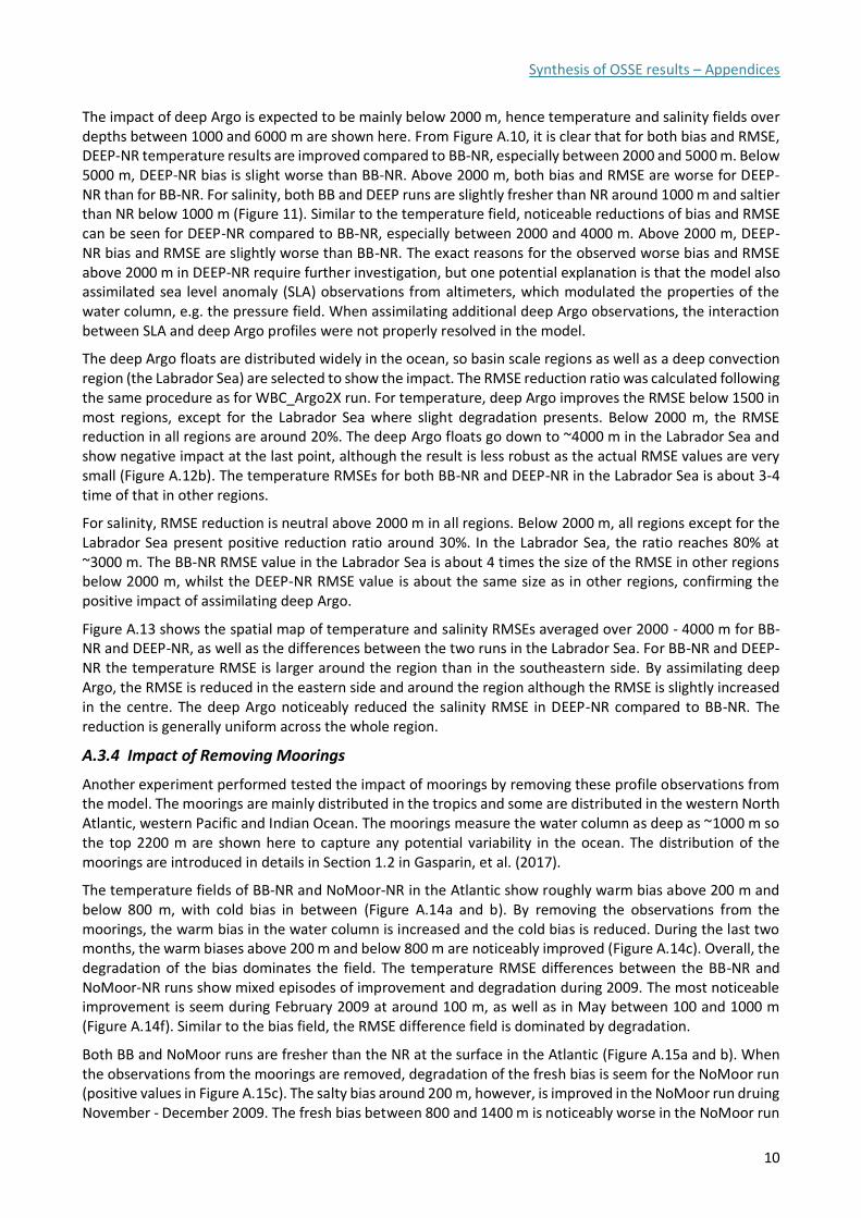
Synthesis of OSSE results – Appendices
10
The impact of deep Argo is expected to be mainly below 2000 m, hence temperature and salinity fields over depths between 1000 and 6000 m are shown here. From Figure A.10, it is clear that for both bias and RMSE, DEEP-NR temperature results are improved compared to BB-NR, especially between 2000 and 5000 m. Below 5000 m, DEEP-NR bias is slight worse than BB-NR. Above 2000 m, both bias and RMSE are worse for DEEP-NR than for BB-NR. For salinity, both BB and DEEP runs are slightly fresher than NR around 1000 m and saltier than NR below 1000 m (Figure 11). Similar to the temperature field, noticeable reductions of bias and RMSE can be seen for DEEP-NR compared to BB-NR, especially between 2000 and 4000 m. Above 2000 m, DEEP-NR bias and RMSE are slightly worse than BB-NR. The exact reasons for the observed worse bias and RMSE above 2000 m in DEEP-NR require further investigation, but one potential explanation is that the model also assimilated sea level anomaly (SLA) observations from altimeters, which modulated the properties of the water column, e.g. the pressure field. When assimilating additional deep Argo observations, the interaction between SLA and deep Argo profiles were not properly resolved in the model.
The deep Argo floats are distributed widely in the ocean, so basin scale regions as well as a deep convection region (the Labrador Sea) are selected to show the impact. The RMSE reduction ratio was calculated following the same procedure as for WBC_Argo2X run. For temperature, deep Argo improves the RMSE below 1500 in most regions, except for the Labrador Sea where slight degradation presents. Below 2000 m, the RMSE reduction in all regions are around 20%. The deep Argo floats go down to ~4000 m in the Labrador Sea and show negative impact at the last point, although the result is less robust as the actual RMSE values are very small (Figure A.12b). The temperature RMSEs for both BB-NR and DEEP-NR in the Labrador Sea is about 3-4 time of that in other regions.
For salinity, RMSE reduction is neutral above 2000 m in all regions. Below 2000 m, all regions except for the Labrador Sea present positive reduction ratio around 30%. In the Labrador Sea, the ratio reaches 80% at ~3000 m. The BB-NR RMSE value in the Labrador Sea is about 4 times the size of the RMSE in other regions below 2000 m, whilst the DEEP-NR RMSE value is about the same size as in other regions, confirming the positive impact of assimilating deep Argo.
Figure A.13 shows the spatial map of temperature and salinity RMSEs averaged over 2000 - 4000 m for BB-NR and DEEP-NR, as well as the differences between the two runs in the Labrador Sea. For BB-NR and DEEP-NR the temperature RMSE is larger around the region than in the southeastern side. By assimilating deep Argo, the RMSE is reduced in the eastern side and around the region although the RMSE is slightly increased in the centre. The deep Argo noticeably reduced the salinity RMSE in DEEP-NR compared to BB-NR. The reduction is generally uniform across the whole region.
A.3.4 Impact of Removing Moorings
Another experiment performed tested the impact of moorings by removing these profile observations from the model. The moorings are mainly distributed in the tropics and some are distributed in the western North Atlantic, western Pacific and Indian Ocean. The moorings measure the water column as deep as ~1000 m so the top 2200 m are shown here to capture any potential variability in the ocean. The distribution of the moorings are introduced in details in Section 1.2 in Gasparin, et al. (2017).
The temperature fields of BB-NR and NoMoor-NR in the Atlantic show roughly warm bias above 200 m and below 800 m, with cold bias in between (Figure A.14a and b). By removing the observations from the moorings, the warm bias in the water column is increased and the cold bias is reduced. During the last two months, the warm biases above 200 m and below 800 m are noticeably improved (Figure A.14c). Overall, the degradation of the bias dominates the field. The temperature RMSE differences between the BB-NR and NoMoor-NR runs show mixed episodes of improvement and degradation during 2009. The most noticeable improvement is seem during February 2009 at around 100 m, as well as in May between 100 and 1000 m (Figure A.14f). Similar to the bias field, the RMSE difference field is dominated by degradation.
Both BB and NoMoor runs are fresher than the NR at the surface in the Atlantic (Figure A.15a and b). When the observations from the moorings are removed, degradation of the fresh bias is seem for the NoMoor run (positive values in Figure A.15c). The salty bias around 200 m, however, is improved in the NoMoor run druing November - December 2009. The fresh bias between 800 and 1400 m is noticeably worse in the NoMoor run
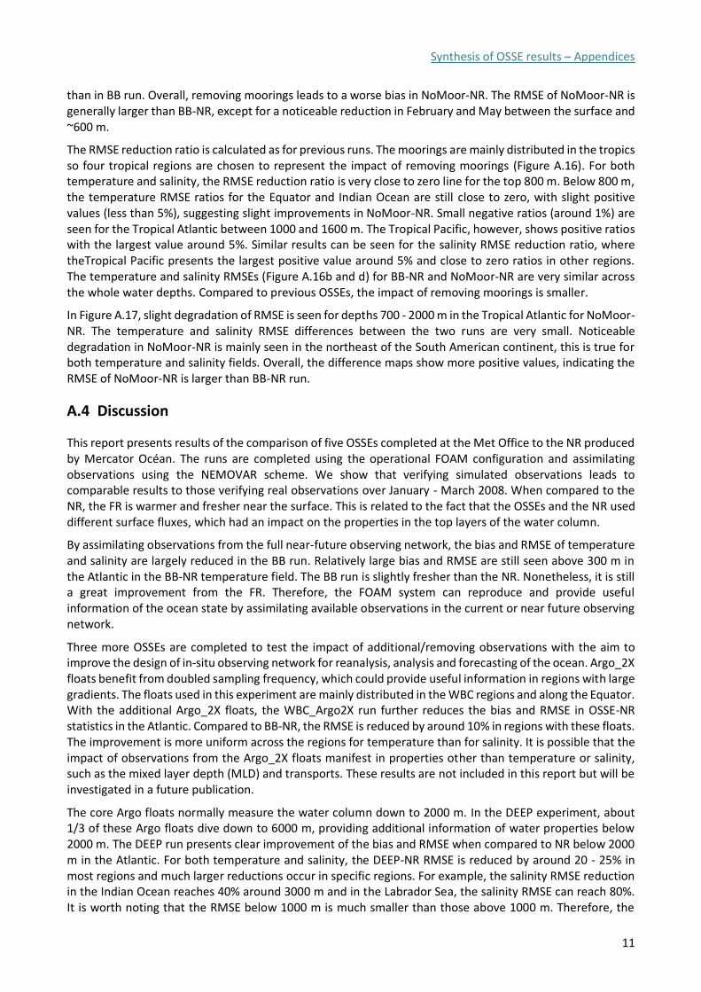
Synthesis of OSSE results – Appendices
11
than in BB run. Overall, removing moorings leads to a worse bias in NoMoor-NR. The RMSE of NoMoor-NR is generally larger than BB-NR, except for a noticeable reduction in February and May between the surface and ~600 m.
The RMSE reduction ratio is calculated as for previous runs. The moorings are mainly distributed in the tropics so four tropical regions are chosen to represent the impact of removing moorings (Figure A.16). For both temperature and salinity, the RMSE reduction ratio is very close to zero line for the top 800 m. Below 800 m, the temperature RMSE ratios for the Equator and Indian Ocean are still close to zero, with slight positive values (less than 5%), suggesting slight improvements in NoMoor-NR. Small negative ratios (around 1%) are seen for the Tropical Atlantic between 1000 and 1600 m. The Tropical Pacific, however, shows positive ratios with the largest value around 5%. Similar results can be seen for the salinity RMSE reduction ratio, where theTropical Pacific presents the largest positive value around 5% and close to zero ratios in other regions. The temperature and salinity RMSEs (Figure A.16b and d) for BB-NR and NoMoor-NR are very similar across the whole water depths. Compared to previous OSSEs, the impact of removing moorings is smaller.
In Figure A.17, slight degradation of RMSE is seen for depths 700 - 2000 m in the Tropical Atlantic for NoMoor-NR. The temperature and salinity RMSE differences between the two runs are very small. Noticeable degradation in NoMoor-NR is mainly seen in the northeast of the South American continent, this is true for both temperature and salinity fields. Overall, the difference maps show more positive values, indicating the RMSE of NoMoor-NR is larger than BB-NR run.
A.4 Discussion
This report presents results of the comparison of five OSSEs completed at the Met Office to the NR produced by Mercator Océan. The runs are completed using the operational FOAM configuration and assimilating observations using the NEMOVAR scheme. We show that verifying simulated observations leads to comparable results to those verifying real observations over January - March 2008. When compared to the NR, the FR is warmer and fresher near the surface. This is related to the fact that the OSSEs and the NR used different surface fluxes, which had an impact on the properties in the top layers of the water column.
By assimilating observations from the full near-future observing network, the bias and RMSE of temperature and salinity are largely reduced in the BB run. Relatively large bias and RMSE are still seen above 300 m in the Atlantic in the BB-NR temperature field. The BB run is slightly fresher than the NR. Nonetheless, it is still a great improvement from the FR. Therefore, the FOAM system can reproduce and provide useful information of the ocean state by assimilating available observations in the current or near future observing network.
Three more OSSEs are completed to test the impact of additional/removing observations with the aim to improve the design of in-situ observing network for reanalysis, analysis and forecasting of the ocean. Argo_2X floats benefit from doubled sampling frequency, which could provide useful information in regions with large gradients. The floats used in this experiment are mainly distributed in the WBC regions and along the Equator. With the additional Argo_2X floats, the WBC_Argo2X run further reduces the bias and RMSE in OSSE-NR statistics in the Atlantic. Compared to BB-NR, the RMSE is reduced by around 10% in regions with these floats. The improvement is more uniform across the regions for temperature than for salinity. It is possible that the impact of observations from the Argo_2X floats manifest in properties other than temperature or salinity, such as the mixed layer depth (MLD) and transports. These results are not included in this report but will be investigated in a future publication.
The core Argo floats normally measure the water column down to 2000 m. In the DEEP experiment, about 1/3 of these Argo floats dive down to 6000 m, providing additional information of water properties below 2000 m. The DEEP run presents clear improvement of the bias and RMSE when compared to NR below 2000 m in the Atlantic. For both temperature and salinity, the DEEP-NR RMSE is reduced by around 20 - 25% in most regions and much larger reductions occur in specific regions. For example, the salinity RMSE reduction in the Indian Ocean reaches 40% around 3000 m and in the Labrador Sea, the salinity RMSE can reach 80%. It is worth noting that the RMSE below 1000 m is much smaller than those above 1000 m. Therefore, the
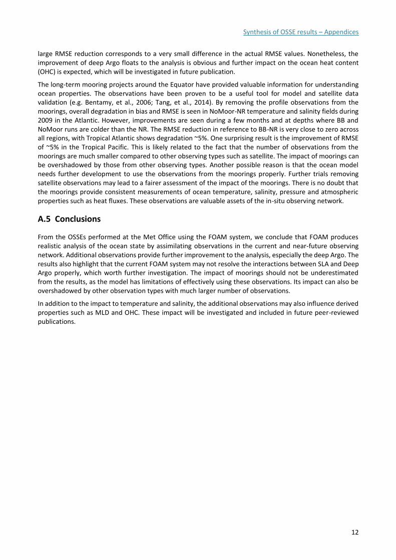
Synthesis of OSSE results – Appendices
12
large RMSE reduction corresponds to a very small difference in the actual RMSE values. Nonetheless, the improvement of deep Argo floats to the analysis is obvious and further impact on the ocean heat content (OHC) is expected, which will be investigated in future publication.
The long-term mooring projects around the Equator have provided valuable information for understanding ocean properties. The observations have been proven to be a useful tool for model and satellite data validation (e.g. Bentamy, et al., 2006; Tang, et al., 2014). By removing the profile observations from the moorings, overall degradation in bias and RMSE is seen in NoMoor-NR temperature and salinity fields during 2009 in the Atlantic. However, improvements are seen during a few months and at depths where BB and NoMoor runs are colder than the NR. The RMSE reduction in reference to BB-NR is very close to zero across all regions, with Tropical Atlantic shows degradation ~5%. One surprising result is the improvement of RMSE of ~5% in the Tropical Pacific. This is likely related to the fact that the number of observations from the moorings are much smaller compared to other observing types such as satellite. The impact of moorings can be overshadowed by those from other observing types. Another possible reason is that the ocean model needs further development to use the observations from the moorings properly. Further trials removing satellite observations may lead to a fairer assessment of the impact of the moorings. There is no doubt that the moorings provide consistent measurements of ocean temperature, salinity, pressure and atmospheric properties such as heat fluxes. These observations are valuable assets of the in-situ observing network.
A.5 Conclusions
From the OSSEs performed at the Met Office using the FOAM system, we conclude that FOAM produces realistic analysis of the ocean state by assimilating observations in the current and near-future observing network. Additional observations provide further improvement to the analysis, especially the deep Argo. The results also highlight that the current FOAM system may not resolve the interactions between SLA and Deep Argo properly, which worth further investigation. The impact of moorings should not be underestimated from the results, as the model has limitations of effectively using these observations. Its impact can also be overshadowed by other observation types with much larger number of observations.
In addition to the impact to temperature and salinity, the additional observations may also influence derived properties such as MLD and OHC. These impact will be investigated and included in future peer-reviewed publications.
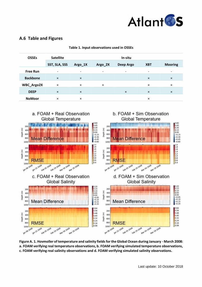
Last update: 10 October 2018
A.6 Table and Figures
Table 1. Input observations used in OSSEs
OSSEs Satellite In-situ
SST, SLA, SSS Argo_1X Argo_2X Deep Argo XBT Mooring
Free Run - - - - - -
Backbone × × × ×
WBC_Argo2X × × × × ×
DEEP × × × × ×
NoMoor × × ×
Figure A. 1. Hovmoller of temperature and salinity fields for the Global Ocean during January - March 2008: a. FOAM verifying real temperature observations, b. FOAM verifying simulated temperature observations, c. FOAM verifying real salinity observations and d. FOAM verifying simulated salinity observations.
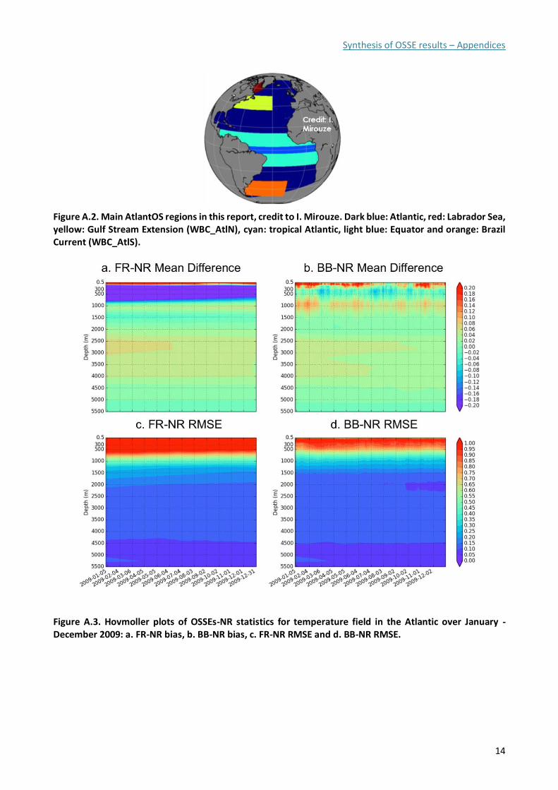
Synthesis of OSSE results – Appendices
14
Figure A.2. Main AtlantOS regions in this report, credit to I. Mirouze. Dark blue: Atlantic, red: Labrador Sea, yellow: Gulf Stream Extension (WBC_AtlN), cyan: tropical Atlantic, light blue: Equator and orange: Brazil Current (WBC_AtlS).
Figure A.3. Hovmoller plots of OSSEs-NR statistics for temperature field in the Atlantic over January - December 2009: a. FR-NR bias, b. BB-NR bias, c. FR-NR RMSE and d. BB-NR RMSE.
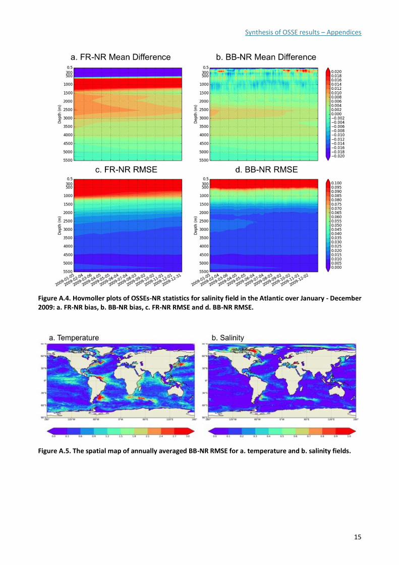
Synthesis of OSSE results – Appendices
15
Figure A.4. Hovmoller plots of OSSEs-NR statistics for salinity field in the Atlantic over January - December 2009: a. FR-NR bias, b. BB-NR bias, c. FR-NR RMSE and d. BB-NR RMSE.
Figure A.5. The spatial map of annually averaged BB-NR RMSE for a. temperature and b. salinity fields.
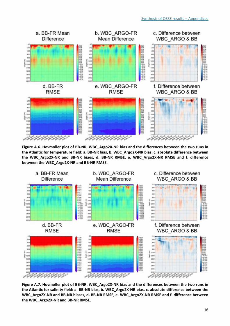
Synthesis of OSSE results – Appendices
16
Figure A.6. Hovmoller plot of BB-NR, WBC_Argo2X-NR bias and the differences between the two runs in the Atlantic for temperature field: a. BB-NR bias, b. WBC_Argo2X-NR bias, c. absolute difference between the WBC_Argo2X-NR and BB-NR biaes, d. BB-NR RMSE, e. WBC_Argo2X-NR RMSE and f. difference between the WBC_Argo2X-NR and BB-NR RMSE.
Figure A.7. Hovmoller plot of BB-NR, WBC_Argo2X-NR bias and the differences between the two runs in the Atlantic for salinity field: a. BB-NR bias, b. WBC_Argo2X-NR bias, c. absolute difference between the WBC_Argo2X-NR and BB-NR biases, d. BB-NR RMSE, e. WBC_Argo2X-NR RMSE and f. difference between the WBC_Argo2X-NR and BB-NR RMSE.
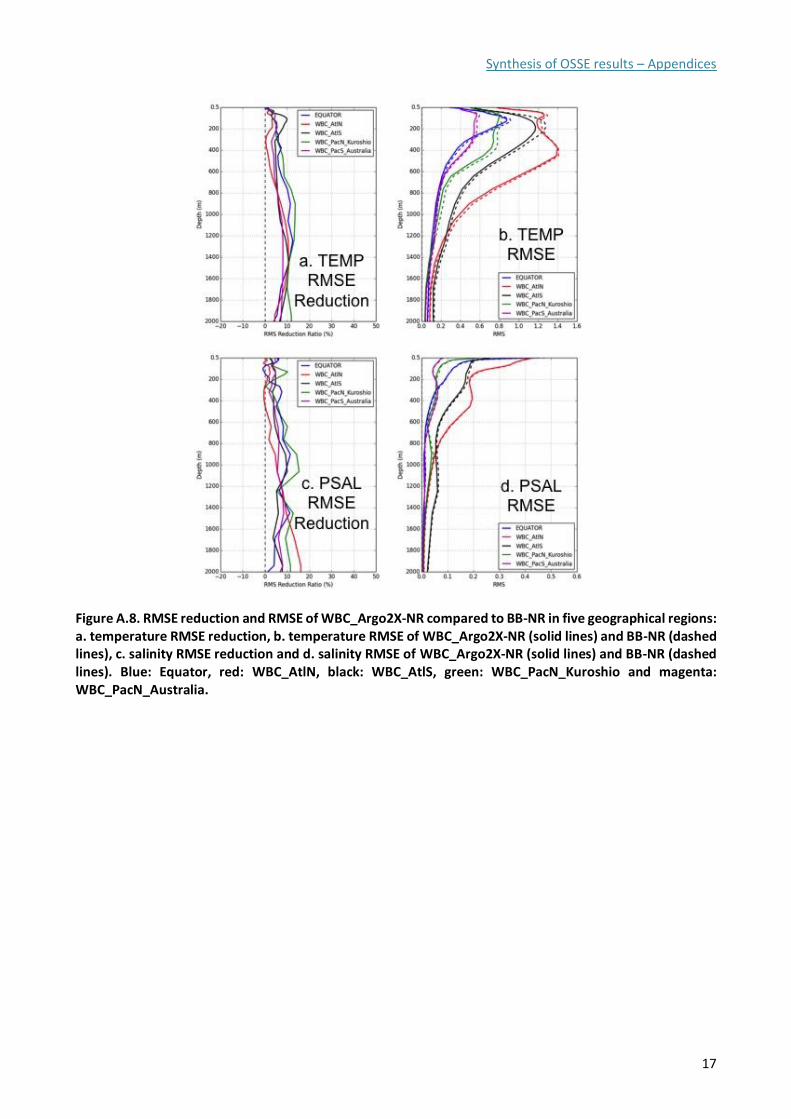
Synthesis of OSSE results – Appendices
17
Figure A.8. RMSE reduction and RMSE of WBC_Argo2X-NR compared to BB-NR in five geographical regions: a. temperature RMSE reduction, b. temperature RMSE of WBC_Argo2X-NR (solid lines) and BB-NR (dashed lines), c. salinity RMSE reduction and d. salinity RMSE of WBC_Argo2X-NR (solid lines) and BB-NR (dashed lines). Blue: Equator, red: WBC_AtlN, black: WBC_AtlS, green: WBC_PacN_Kuroshio and magenta: WBC_PacN_Australia.
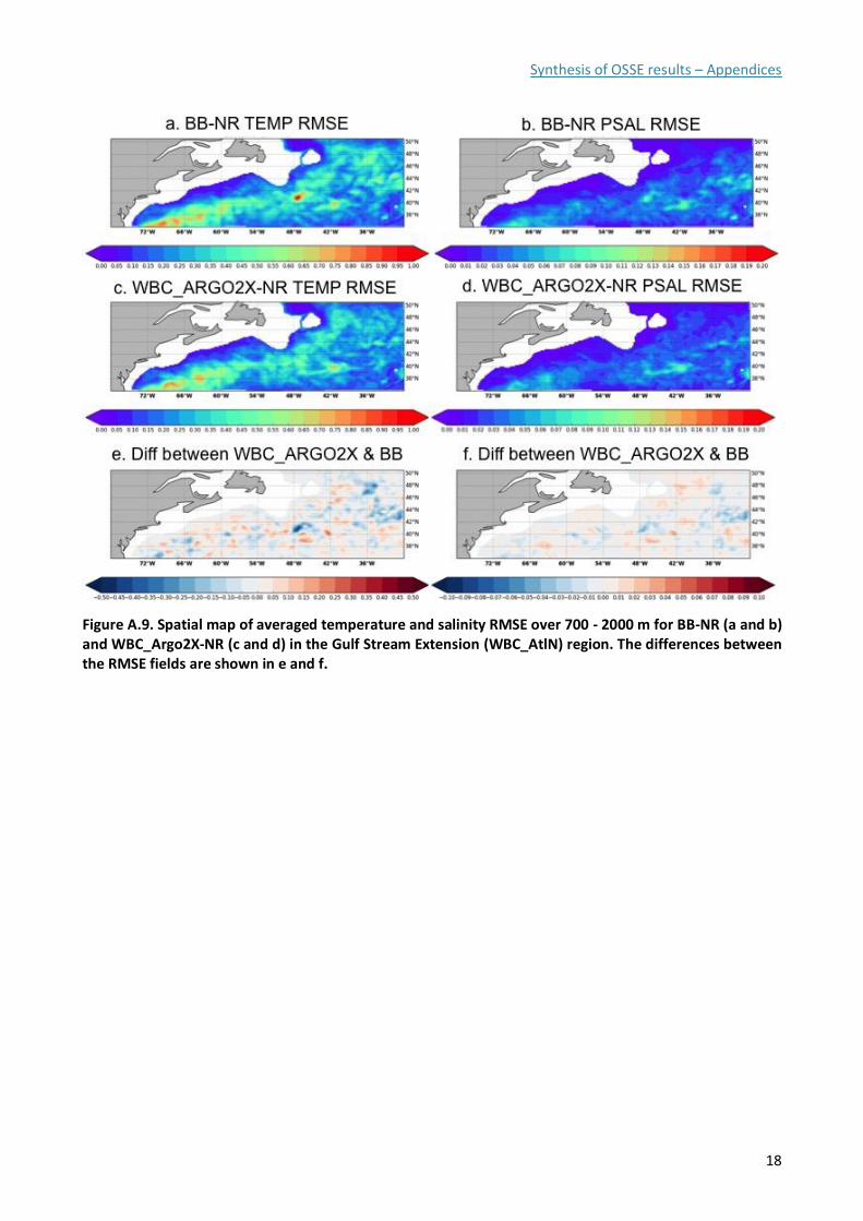
Synthesis of OSSE results – Appendices
18
Figure A.9. Spatial map of averaged temperature and salinity RMSE over 700 - 2000 m for BB-NR (a and b) and WBC_Argo2X-NR (c and d) in the Gulf Stream Extension (WBC_AtlN) region. The differences between the RMSE fields are shown in e and f.
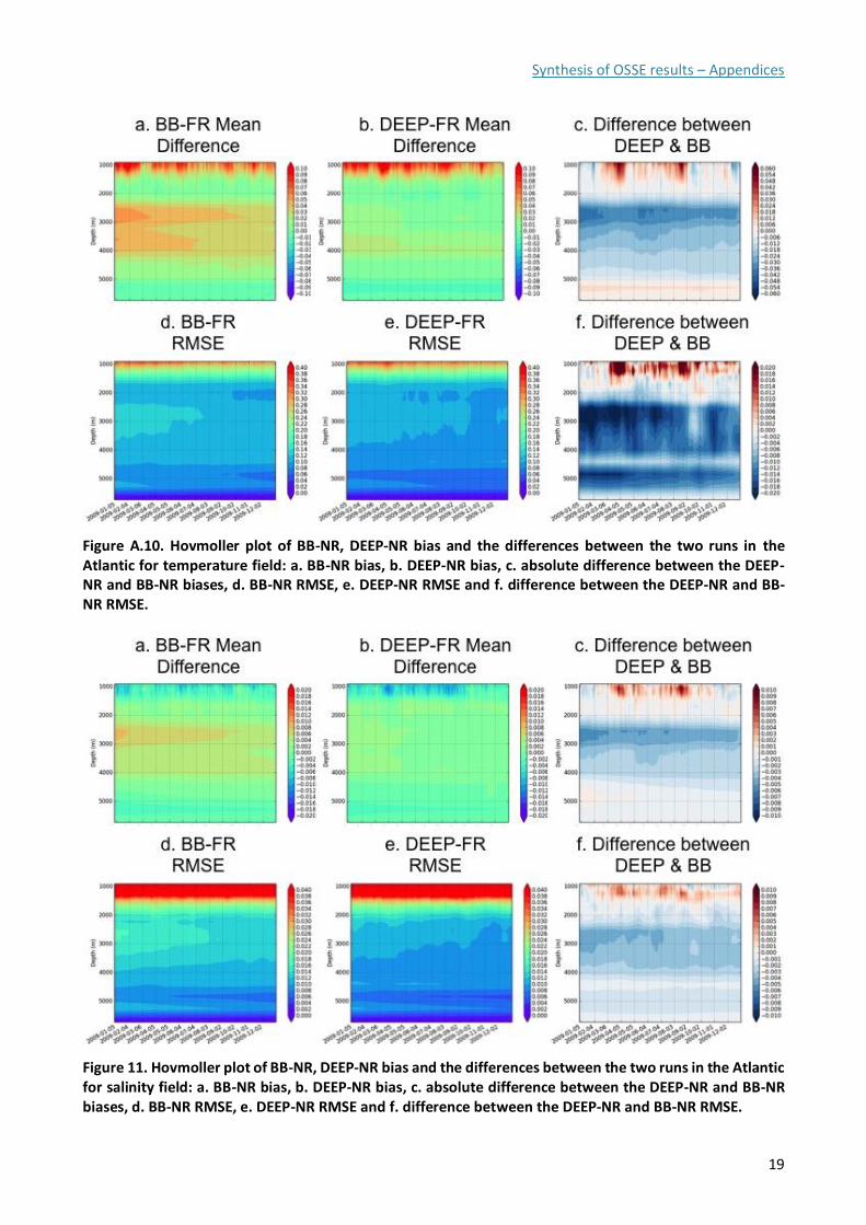
Synthesis of OSSE results – Appendices
19
Figure A.10. Hovmoller plot of BB-NR, DEEP-NR bias and the differences between the two runs in the Atlantic for temperature field: a. BB-NR bias, b. DEEP-NR bias, c. absolute difference between the DEEP-NR and BB-NR biases, d. BB-NR RMSE, e. DEEP-NR RMSE and f. difference between the DEEP-NR and BB-NR RMSE.
Figure 11. Hovmoller plot of BB-NR, DEEP-NR bias and the differences between the two runs in the Atlantic for salinity field: a. BB-NR bias, b. DEEP-NR bias, c. absolute difference between the DEEP-NR and BB-NR biases, d. BB-NR RMSE, e. DEEP-NR RMSE and f. difference between the DEEP-NR and BB-NR RMSE.
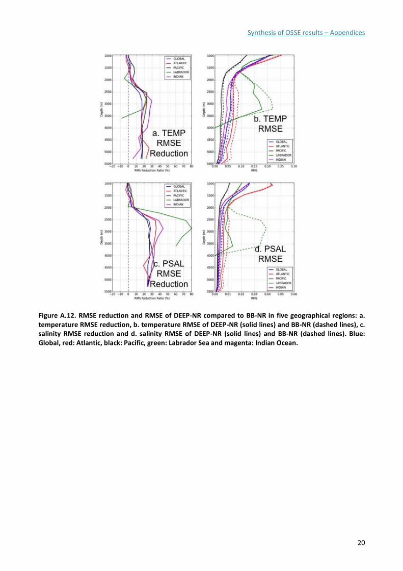
Synthesis of OSSE results – Appendices
20
Figure A.12. RMSE reduction and RMSE of DEEP-NR compared to BB-NR in five geographical regions: a. temperature RMSE reduction, b. temperature RMSE of DEEP-NR (solid lines) and BB-NR (dashed lines), c. salinity RMSE reduction and d. salinity RMSE of DEEP-NR (solid lines) and BB-NR (dashed lines). Blue: Global, red: Atlantic, black: Pacific, green: Labrador Sea and magenta: Indian Ocean.
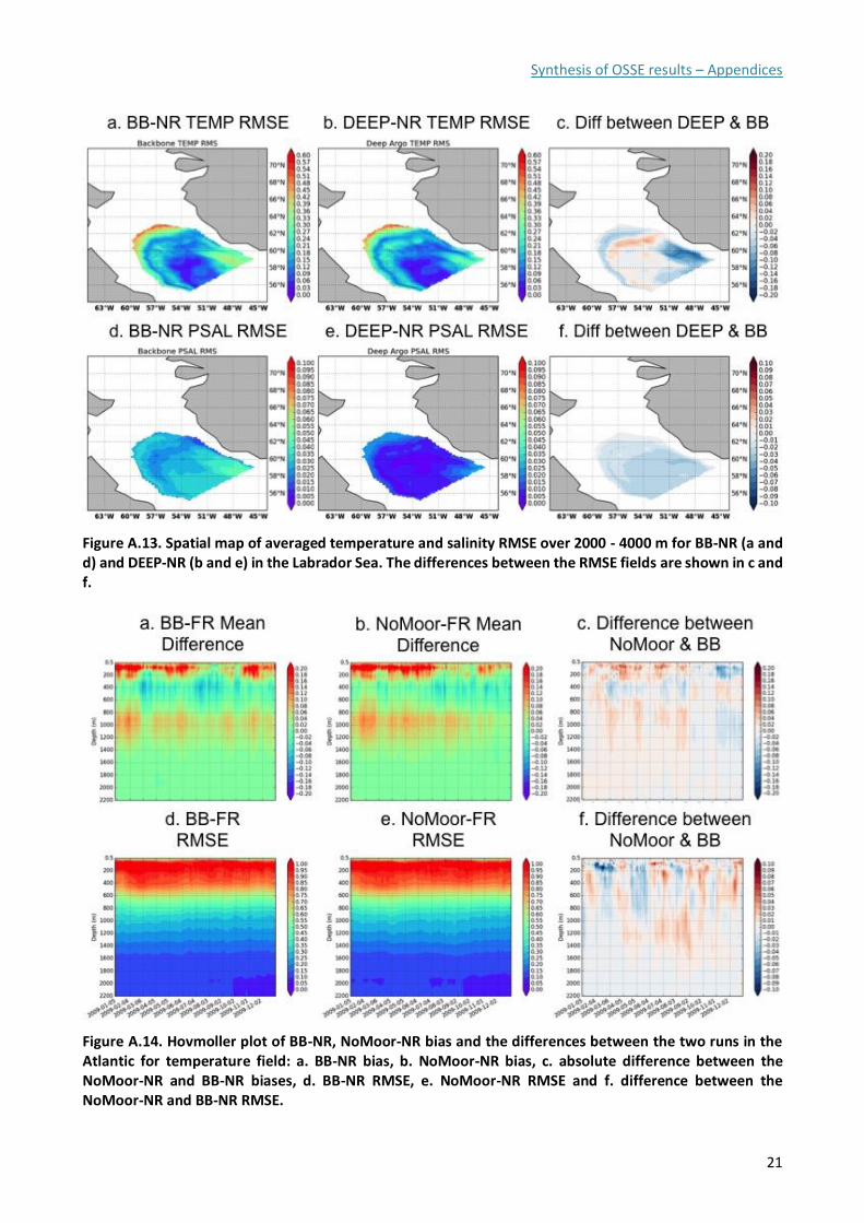
Synthesis of OSSE results – Appendices
21
Figure A.13. Spatial map of averaged temperature and salinity RMSE over 2000 - 4000 m for BB-NR (a and d) and DEEP-NR (b and e) in the Labrador Sea. The differences between the RMSE fields are shown in c and f.
Figure A.14. Hovmoller plot of BB-NR, NoMoor-NR bias and the differences between the two runs in the Atlantic for temperature field: a. BB-NR bias, b. NoMoor-NR bias, c. absolute difference between the NoMoor-NR and BB-NR biases, d. BB-NR RMSE, e. NoMoor-NR RMSE and f. difference between the NoMoor-NR and BB-NR RMSE.
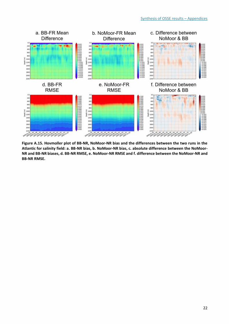
Synthesis of OSSE results – Appendices
22
Figure A.15. Hovmoller plot of BB-NR, NoMoor-NR bias and the differences between the two runs in the Atlantic for salinity field: a. BB-NR bias, b. NoMoor-NR bias, c. absolute difference between the NoMoor-NR and BB-NR biases, d. BB-NR RMSE, e. NoMoor-NR RMSE and f. difference between the NoMoor-NR and BB-NR RMSE.
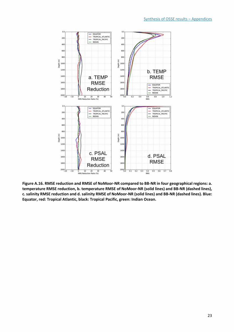
Synthesis of OSSE results – Appendices
23
Figure A.16. RMSE reduction and RMSE of NoMoor-NR compared to BB-NR in four geographical regions: a. temperature RMSE reduction, b. temperature RMSE of NoMoor-NR (solid lines) and BB-NR (dashed lines), c. salinity RMSE reduction and d. salinity RMSE of NoMoor-NR (solid lines) and BB-NR (dashed lines). Blue: Equator, red: Tropical Atlantic, black: Tropical Pacific, green: Indian Ocean.
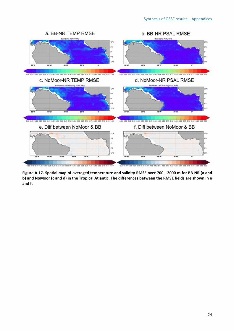
Synthesis of OSSE results – Appendices
24
Figure A.17. Spatial map of averaged temperature and salinity RMSE over 700 - 2000 m for BB-NR (a and b) and NoMoor (c and d) in the Tropical Atlantic. The differences between the RMSE fields are shown in e and f.
Last update: 10 October 2018
A.8 References
Bentamy, A., F. Girard-Ardhuin, D. Croizé-Fillon, and P. Queffeulou. 2006. Validation and Analysis of Ocean Parameters Using ASCAT Data. IFREMER.
Cao, C., X. Xiong, R. Wolfe, F. DeLuccia, Q. Liu, S. Blonski, G. Lin, et al. 2013. Visible Infrared Imaging Radiometer Suite (VIIRS) Sensor Data Record (SDR) User's Guide. NOAA/NESDIS/STAR.
Ebita, A., S. Kobayashi, Y. Ota, M. Moriya, R. Kumabe, K. Onogi, Y. Harada, et al. 2011. “The Japanese 55-year Reanalysis "JRA-55": An Interim Report.” Science Online Letters on the Atmosphere. https://www.jstage.jst.go.jp/article/sola/7/0/7_0_149/_article.
EUMETSAT. 2011. Single Sensor Error Statistic Scheme for IASI L2P Sea Surface Temperature. EUMETSAT.
Gasparin, F., E. Remy, M. Hamon, C. Regnier, and S. Guinehut. 2017. Information about Synthetic Data Files for AtlantOS OSSE. Toulouse: Mercator-Océan.
Kobayashi, S., Y. Ota, Y. Harada, A. Ebita, M. Moriya, H. Onoda, K. Onogi, et al. 2015. “The JRA-55 Reanalysis: General Specifications and Basic Characteristics.” Journal of the Meteorological Society of Japan 5-48.
Kubota, M., and H. Tomita. 2015. “Results from intercomparison of various turbulent heat fluxes.” Workshop on Energy Flow Through the Climate System. Exeter, UK: the Met Office.
Lellouche, J-M., O. Legalloudec, C. Regnier, B. Levierand, E. Greiner, and M. Drevillon. 2016. Quality Information Document for Global Sea Physical Analysis and Forecasting Product. Rome: CMEMS.
Merchant, C., and C. Bulgin. 2014. Uncertainty Characterisation Report: Sea Surface Temperature v1. Reading, UK: University of Reading.
NOAA/NESDIS/STAR. n.d. AVHRR NEDTs. https://www.star.nesdis.noaa.gov/sod/sst/3s/#single-chart.
Tang, W., S. H. Yueh, A. G. Fore, and A. Hayashi. 2014. “Validation of Aquarius Sea Surface Salinity with in situ measurements from Argo floats and moored buoys.” Journal of Geophysical Research: Oceans 6171-6189.
Tsamalis, C. 2017. “The quality of Sea Surface Temperature observations from drifting buoys and the role of the natural variability.” Fiducial Reference Measurements for satellite derived surface temperature product validation (FRM4STS) international workshop. Teddington, UK.
Wang, X. L., Y. Feng, R. Chan, and V. Isaac. 2016. “Inter-comparison of Extra-tropical Cyclone Activity in Nine Reanalysis Datasets.” Atmospheric Research 133-153.
Waters, J., D. J. Lea, M. J. Martin, I. Mirouze, A. Weaver, and J. While. 2015. “Implementing a variational data assimilation system in an operational 1/4 degree global ocean model.” Quarterly Journal of the Royal Meteorological Society 333-349.
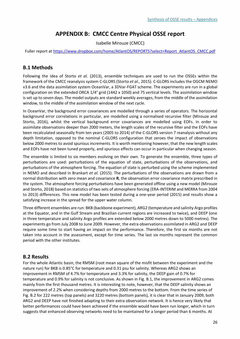
Synthesis of OSSE results – Appendices
26
APPENDIX B: CMCC Centre Physical OSSE report
Isabelle Mirouze (CMCC)
Fuller report at https://www.dropbox.com/home/AtlantOS/REPORTS?select=Report_AtlantOS_CMCC.pdf
B.1 Methods
Following the idea of Storto et al. (2013), ensemble techniques are used to run the OSSEs within the framework of the CMCC reanalysis system C-GLORS (Storto et al., 2015). C-GLORS includes the OGCM NEMO v3.6 and the data assimilation system OceanVar, a 3DVar-FGAT scheme. The experiments are run in a global configuration on the extended ORCA 1/4° grid (1442 x 1050) and 75 vertical levels. The assimilation window is set up to seven days. The model outputs are standard weekly averages, from the middle of the assimilation window, to the middle of the assimilation window of the next cycle.
In OceanVar, the background error covariances are modelled through a series of operators. The horizontal background error correlations in particular, are modelled using a normalised recursive filter (Mirouze and Storto, 2016), whilst the vertical background error covariances are modelled using EOFs. In order to assimilate observations deeper than 2000 meters, the length scales of the recursive filter and the EOFs have been recalculated seasonally from ten years (2005 to 2014) of the C-GLORS version 7 reanalysis without any depth limitation, opposed to the nominal C-GLORS configuration that zeroes the impact of observations below 2000 metres to avoid spurious increments. It is worth mentioning however, that the new length scales and EOFs have not been tuned properly, and spurious effects can occur in particular when changing season.
The ensemble is limited to six members evolving on their own. To generate the ensemble, three types of perturbations are used: perturbations of the equation of state, perturbations of the observations, and perturbations of the atmosphere forcing. The equation of state is perturbed using the scheme implemented in NEMO and described in Brankart et al. (2015). The perturbations of the observations are drawn from a normal distribution with zero mean and covariance R, the observation error covariance matrix prescribed in the system. The atmosphere forcing perturbations have been generated offline using a new model (Mirouze and Storto, 2018) based on statistics of two sets of atmosphere forcing (ERA-INTERIM and MERRA from 2004 to 2013) differences. This new model has been tested during a one-year period (2015) and results show a satisfying increase in the spread for the upper water column.
Three different ensembles are run: BKB (backbone experiment), ARG2 (temperature and salinity Argo profiles at the Equator, and in the Gulf Stream and Brazilian current regions are increased to twice), and DEEP (one in three temperature and salinity Argo profiles are extended below 2000 metres down to 5000 metres). The experiments go from July 2008 to June 2009. However, the extra observations assimilated in ARG2 and DEEP require some time to start having an impact on the performance. Therefore, the first six months are not taken into account in the assessment, except for time series. The last six months represent the common period with the other institutes.
B.2 Results
For the whole Atlantic basin, the RMSM (root mean square of the misfit between the experiment and the nature run) for BKB is 0.85°C for temperature and 0.31 psu for salinity. Whereas ARG2 shows an improvement in RMSM of 4.7% for temperature and 3.3% for salinity, the DEEP gain of 0.7% for temperature and 0.9% for salinity is not conclusive. As shown in Fig. B.1, the improvement in ARG2 comes mainly from the first thousand metres. It is interesting to note, however, that the DEEP salinity shows an improvement of 2.2% when considering depths from 2000 metres to the bottom. From the time series of Fig. B.2 for 222 metres (top panels) and 3220 metres (bottom panels), it is clear that in January 2009, both ARG2 and DEEP have not finished adapting to their extra observation network. It is hence very likely that better performances could have been achieved if the ensemble would have been run longer, which in turn suggests that enhanced observing networks need to be maintained for a longer period than 6 months. At
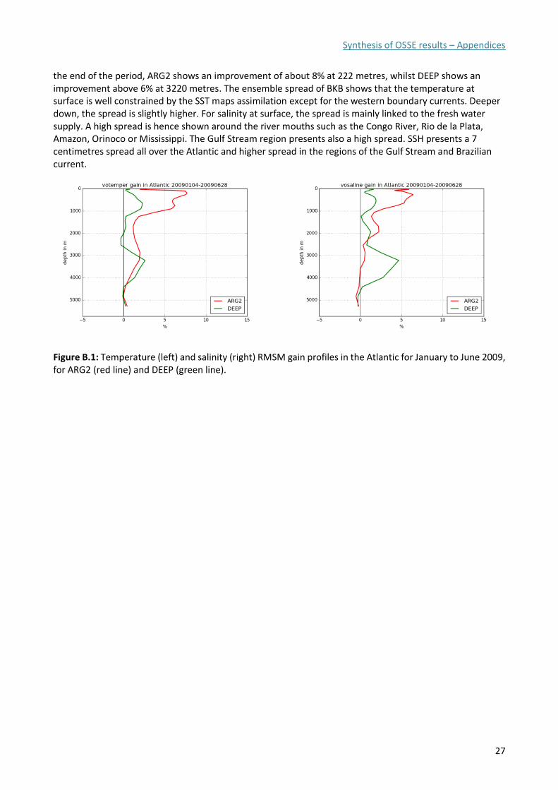
Synthesis of OSSE results – Appendices
27
the end of the period, ARG2 shows an improvement of about 8% at 222 metres, whilst DEEP shows an improvement above 6% at 3220 metres. The ensemble spread of BKB shows that the temperature at surface is well constrained by the SST maps assimilation except for the western boundary currents. Deeper down, the spread is slightly higher. For salinity at surface, the spread is mainly linked to the fresh water supply. A high spread is hence shown around the river mouths such as the Congo River, Rio de la Plata, Amazon, Orinoco or Mississippi. The Gulf Stream region presents also a high spread. SSH presents a 7 centimetres spread all over the Atlantic and higher spread in the regions of the Gulf Stream and Brazilian current.
Figure B.1: Temperature (left) and salinity (right) RMSM gain profiles in the Atlantic for January to June 2009, for ARG2 (red line) and DEEP (green line).
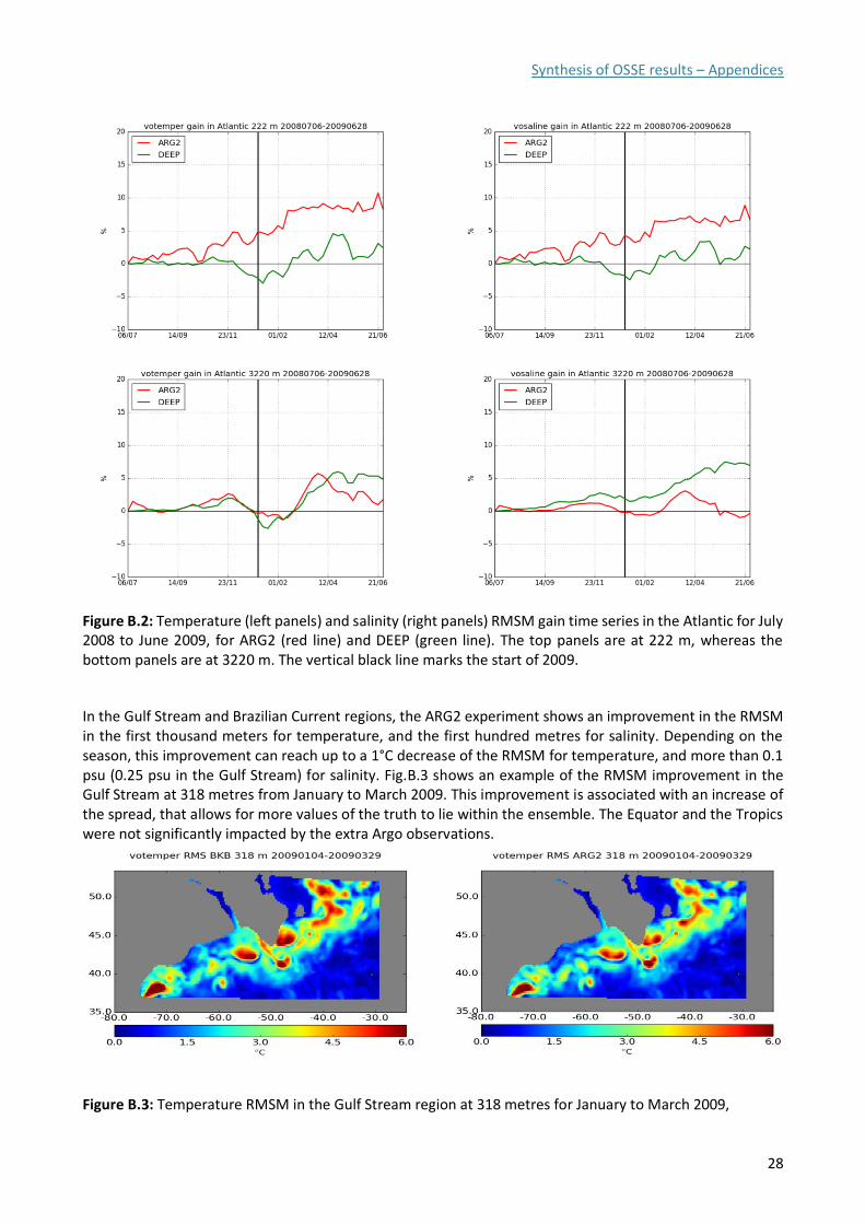
Synthesis of OSSE results – Appendices
28
Figure B.2: Temperature (left panels) and salinity (right panels) RMSM gain time series in the Atlantic for July 2008 to June 2009, for ARG2 (red line) and DEEP (green line). The top panels are at 222 m, whereas the bottom panels are at 3220 m. The vertical black line marks the start of 2009.
In the Gulf Stream and Brazilian Current regions, the ARG2 experiment shows an improvement in the RMSM in the first thousand meters for temperature, and the first hundred metres for salinity. Depending on the season, this improvement can reach up to a 1°C decrease of the RMSM for temperature, and more than 0.1 psu (0.25 psu in the Gulf Stream) for salinity. Fig.B.3 shows an example of the RMSM improvement in the Gulf Stream at 318 metres from January to March 2009. This improvement is associated with an increase of the spread, that allows for more values of the truth to lie within the ensemble. The Equator and the Tropics were not significantly impacted by the extra Argo observations.
Figure B.3: Temperature RMSM in the Gulf Stream region at 318 metres for January to March 2009,
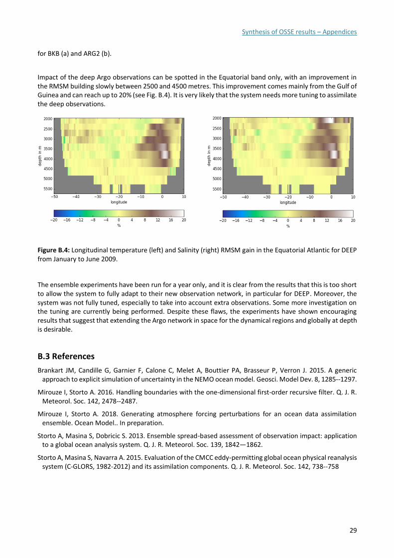
Synthesis of OSSE results – Appendices
29
for BKB (a) and ARG2 (b).
Impact of the deep Argo observations can be spotted in the Equatorial band only, with an improvement in the RMSM building slowly between 2500 and 4500 metres. This improvement comes mainly from the Gulf of Guinea and can reach up to 20% (see Fig. B.4). It is very likely that the system needs more tuning to assimilate the deep observations.
Figure B.4: Longitudinal temperature (left) and Salinity (right) RMSM gain in the Equatorial Atlantic for DEEP from January to June 2009.
The ensemble experiments have been run for a year only, and it is clear from the results that this is too short to allow the system to fully adapt to their new observation network, in particular for DEEP. Moreover, the system was not fully tuned, especially to take into account extra observations. Some more investigation on the tuning are currently being performed. Despite these flaws, the experiments have shown encouraging results that suggest that extending the Argo network in space for the dynamical regions and globally at depth is desirable.
B.3 References
Brankart JM, Candille G, Garnier F, Calone C, Melet A, Bouttier PA, Brasseur P, Verron J. 2015. A generic approach to explicit simulation of uncertainty in the NEMO ocean model. Geosci. Model Dev. 8, 1285--1297.
Mirouze I, Storto A. 2016. Handling boundaries with the one-dimensional first-order recursive filter. Q. J. R. Meteorol. Soc. 142, 2478--2487.
Mirouze I, Storto A. 2018. Generating atmosphere forcing perturbations for an ocean data assimilation ensemble. Ocean Model.. In preparation.
Storto A, Masina S, Dobricic S. 2013. Ensemble spread-based assessment of observation impact: application to a global ocean analysis system. Q. J. R. Meteorol. Soc. 139, 1842—1862.
Storto A, Masina S, Navarra A. 2015. Evaluation of the CMCC eddy-permitting global ocean physical reanalysis system (C-GLORS, 1982-2012) and its assimilation components. Q. J. R. Meteorol. Soc. 142, 738--758

Synthesis of OSSE results – Appendices
30
Synthesis of OSSE results – Appendices
31
APPENDIX C: OSSE results using the multivariate ARMOR3D data analysis system
Stephanie Guinehut (CLS)
C.1 Introduction
This report is Appendix C to D1.5 on “Synthesis of OSSE results”. It presents results using the multivariate ARMOR3D data analysis system. ARMOR3D is a complementary approach to OSSE studies based on data assimilation systems such as the ones carried out by Mercator Océan, UK MetOffice and CMCC. ARMOR3D is part of CMEMS Multi Observations Thematic Assembly Center (MOB TAC) that rely on the use of statistical methods to combine satellite (SLA, SST, SSS) and in-situ observations (T/S profiles) for an optimal reconstruction of global 3D temperature and salinity gridded fields.
To study the impact of the enhancement of the Atlantic Ocean observing system on ocean state estimate using the ARMOR3D system, as part of task 1.3.1, CLS has carried out the following experiments:
• Backbone experiment,
• ArgoX2 experiment,
• Deep Argo experiment,
• Drifter experiment,
• Mooring experiment.
Results for each of these experiments are summarized in the following sections. The complete and detailed description of the work is available in Sections C.7 – C.9.
C.2 Backbone experiment The Backbone experiment is the reference experiment from which observations are added for most of the other experiments or removed for the Mooring experiment. As for the CMEMS ARMOR3D multiyear system (http://marine.copernicus.eu/documents/PUM/CMEMS-MOB-PUM-015-002.pdf), the Backbone experiment is constructed using satellite L4 observations of SLA, SST and SSS and in-situ observations of T&S profiles from the following array: Argo, XBT, moorings.
It is considered as the reference and results from the other experiments are compared to the results obtained from the Backbone experiment.
C.3 Argo X2 experiment The Argo X2 experiment uses the same observations as the Backbone experiment plus additional in-situ T&S Argo profiles at the Equator and in the Western boundary current regions (i.e. Gulf Stream, Kuroshio, Agulhas, Confluence…) where their number is increased to twice.
As the ARMOR3D method relies on the use of statistical methods with no dynamical propagation, the impact of the Argo X2 experiment is localized where the number of Argo observations is increased to twice. At global scale, the BIAS reduction is maximum at a depth of 100m. Argo X2 experiment allow a better representation of the variability with a MS (Mean Square) reduction up to 20% around 800m depth in the Gulf Stream region for the temperature and salinity fields, of about 10% for the temperature field of the Confluence region and 15% for its salinity field. The MS reduction of the Tropical Atlantic region is much smaller and below 5%, this weaker improvement is because the Tropical Atlantic region is defined between 15°S and 15°N and Argo observations is only increased to twice between 3°S and 3°N. Results show also a positive impact on MLD retrieval.
Synthesis of OSSE results – Appendices
32
C.4 Deep Argo experiment The Deep Argo experiment uses the same observations as the Backbone experiment plus additional in-situ T&S Argo observations below 2000 m down to the bottom. 1/3 of the Argo array have been expended down to the bottom.
Over time the Backbone experiment progressively drifts from the Nature Run (i.e. it is unable to reproduce the interannual variability of the Nature Run). The Deep Argo observations allow for a correction of the bias and the interannual variability of the bias which grows with time. For the temperature field, the most important improvements are in the Southern Ocean and they are in the North Atlantic Ocean for the salinity field. In the ARMOR3D system, the Deep Argo observations do not help to better reproduce other types of variability if any. The MS reduction due to the BIAS reduction is maximum in the Gulf Stream region and the salinity field and is up to 60% at 2000m depth, then decreases to 40% between 3000 and 4000m depth. For the temperature field, the contribution of the Deep Argo observations in the AtlantOS region is up to 30% MS reduction with Backbone at 1750m going down to 10% at 5000m. There is additionally a positive impact on Ocean Heat Content retrieval with a reduction of the bias and the correction of the trend.
C.5 Drifter experiment The Drifter experiment uses the same observations as the Backbone experiment plus additional in-situ observations from an array of surface drifters equipped with a thermistor chain instrumented to measure temperature and salinity from the surface to 150m every 5m. To limit the number of additional observations and the associated noise, only 1 observation per drifter per day has been kept.
As the surface layers of the ARMOR3D fields are already well constrained by the satellite SST observations (and to a lesser extent by the SSS observations), the impact of the additional Drifter observations is maximum between 50 and 150m depth. There is a better restitution of the variability between 50 and 150m depth with a global MS reduction with Backbone of 10%. Impact on MLD reconstruction has also been studied. Improvement is visible where MLD are shallower than the maximum depth of the thermistor chain. As the ARMOR3D method is applied for each vertical level, with no vertical propagation of the information, having additional observations in only part of the layers might introduce inconsistency between the layers. A strong recommendation from the ARMOR3D system would thus be to have complete profiles on the vertical.
C.6 Mooring experiment The mooring experiment uses the same observations as the Backbone experiment less the moorings. Unlike other experiments, observations are removed here and not added.
As for the other experiments, the impact of the Mooring experiment is localized where observations have been removed, very locally at each mooring site. Results show a degradation compared to the Backbone experiment, up to -50% MS error reduction with the Backbone experiment at each mooring site. Those results have not been studied further. In fact, as the ARMOR3D method relies on the use of statistical methods with no dynamical propagation, neither in space nor in time, the method might not be appropriate to analyze the impact of a very localized observing system.
Synthesis of OSSE results – Appendices
33
C.7 Design of the experiments
C.7.1 Nature run and observations The Nature Run (NR) is provided by Mercator Océan. It corresponds to a free run (i.e. forced run by the atmosphere in which no satellite and no in-situ data are assimilated) of the PSY4 system at 1/12° horizontal resolution. PSY4 corresponds to the high-resolution monitoring and forecasting system operating through the Copernicus Marine Service (http://marine.copernicus.eu/documents/PUM/CMEMS-GLO-PUM-001-024.pdf). The NR is initialized in 2006 and three years covering the 2008-2010 period are used in this study. A full description of the NR is available in Gasparin et al. (2018 a, b). To compare the different experiments to the Nature Run, the latter is interpolated on a 1/4° horizontal grid and 33 vertical levels (ARMOR3D vertical levels).
All observations (satellite and in-situ) used in the experiments are simulated from the NR.
The set of in-situ observations has been prepared by Mercator Océan and shared among the different groups (Mercator Océan, UK MetOffice, CMCC and CLS) and is fully described in Gasparin et al. (2018a). It consists of T&S profiles from the following arrays: moorings, XBT, Argo and drifters. For each array, realistic samplings have been chosen and representativity and instrumental errors have been introduced (Gasparin et al., 2018a).
For the satellite observations, CLS has prepared its own set of observations. Sea Level Anomaly (SLA), Sea Surface Temperature (SST) and Sea Surface Salinity (SSS) L4 gridded fields have been extracted from the first layer (0.49 m) of the NR fields. To account for the representativity and instrumental errors, a random shift of plus or minus three days has been applied on the dates of the fields. The impact of this shift has been then estimated by computing the rms of the differences between DAY and DAY+/-3 days over the 2008-2010 period and is meant to be representative of the errors. They are up to 0.1m for SLA, 4°C for SST and 1psu for SSS with geographical distributions very consistent to what expected (i.e. high variability regions associated with high mesoscale activity or high seasonal variability) (Figure C.18).
C.7.2 ARMOR3D system ARMOR3D is part of CMEMS Multi Observations Thematic Assembly Center (MOB TAC) and relies on the use of statistical methods to combine satellite (SLA, SST, SSS) and in-situ observations (T/S profiles) for an optimal reconstruction of global 3D temperature and salinity gridded fields.
The method is fully described in Guinehut et al. (2012) and recently updated in http://marine.copernicus.eu/documents/QUID/CMEMS-MOB-QUID-015-002.pdf, and starts from a first guess climatology. Satellite data (SLA + SST + SSS) are then projected onto the vertical using a multiple linear regression method and covariances deduced from historical observations. This step gives synthetic fields from the surface down to 1500m depth. These synthetic fields are then combined with T&S in-situ profiles using an optimal interpolation method. Analyses are performed at a weekly period on a 1/4° horizontal grid on 24 vertical levels from the surface down to 1500m depth. In a final step, the T/S fields are completed from 1500 to 5500m depth (9 additional vertical levels) using the climatology.
Regarding the different ingredients of the ARMOR3D system:
• All observations: SLA, SST, SSS and in-situ T&S profiles are collocated from the Nature Run as described in C.7.1
• The first guess field is obtained from the WOA13 climatology (monthly in the top 1500 m and annual from 1500 to 5500m). Note that a test was performed using a climatology derived from 9 years of the Nature Run (2007-2015) but this option has been excluded since the computed synthetic fields were too close to the Nature Run fields. Associated errors were unrealistic because they were too small to compare with the ones obtained from the operational ARMOR3D system,

Synthesis of OSSE results – Appendices
34
• All parameters, such as regression coefficient used in the multiple linear regression method or covariances used in the optimal interpolation method, are unchanged compared to the operational ARMOR3D system.
SLA (m)
SST (°C)
SSS (psu)
Figure C.18: rms of the differences between DAY and DAY+/-3 days, over the 2008-2010 period, and for SLA (in m), SST (in
°C) and SSS (in psu).
C.7.3 Experiments To study the impact of the enhancement of the Atlantic Ocean observing system on ocean state estimates using the ARMOR3D system, CLS has carried out the following experiments:
• Backbone experiment,
• ArgoX2 experiment,
• Deep Argo experiment,
• Drifter experiment,
• Mooring experiment.
All experiments have been run globally for the 2008-2010 period. Input observations used in the different experiments are listed in Table C.2.
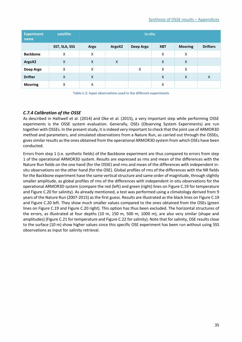
Synthesis of OSSE results – Appendices
35
Experiment name
satellite in-situ
SST, SLA, SSS Argo ArgoX2 Deep Argo XBT Mooring Drifters
Backbone X X X X
ArgoX2 X X X X X
Deep Argo X X X X X
Drifter X X X X X
Mooring X X X
Table C.2: Input observations used in the different experiments
C.7.4 Calibration of the OSSE As described in Halliwell et al. (2014) and Oke et al. (2015), a very important step while performing OSSE experiments is the OSSE system evaluation. Generally, OSEs (Observing System Experiments) are run together with OSSEs. In the present study, it is indeed very important to check that the joint use of ARMOR3D method and parameters, and simulated observations from a Nature Run, as carried out through the OSSEs, gives similar results as the ones obtained from the operational ARMOR3D system from which OSEs have been conducted.
Errors from step 1 (i.e. synthetic fields) of the Backbone experiment are thus compared to errors from step 1 of the operational ARMOR3D system. Results are expressed as rms and mean of the differences with the Nature Run fields on the one hand (for the OSSE) and rms and mean of the differences with independent in-situ observations on the other hand (for the OSE). Global profiles of rms of the differences with the NR fields for the Backbone experiment have the same vertical structure and same order of magnitude, through slightly smaller amplitude, as global profiles of rms of the differences with independent in-situ observations for the operational ARMOR3D system (compare the red (left) and green (right) lines on Figure C.19 for temperature and Figure C.20 for salinity). As already mentioned, a test was performed using a climatology derived from 9 years of the Nature Run (2007-2015) as the first guess. Results are illustrated as the black lines on Figure C.19 and Figure C.20 left. They show much smaller values compared to the ones obtained from the OSEs (green lines on Figure C.19 and Figure C.20 right). This option has thus been excluded. The horizontal structures of the errors, as illustrated at four depths (10 m, 150 m, 500 m, 1000 m), are also very similar (shape and amplitudes) (Figure C.21 for temperature and Figure C.22 for salinity). Note that for salinity, OSE results close to the surface (10 m) show higher values since this specific OSE experiment has been run without using SSS observations as input for salinity retrieval.
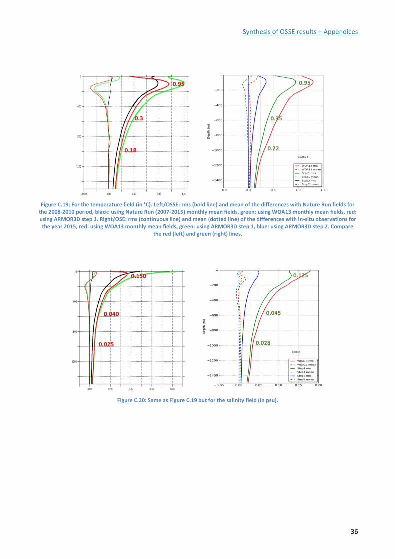
Synthesis of OSSE results – Appendices
36
Figure C.19: For the temperature field (in °C). Left/OSSE: rms (bold line) and mean of the differences with Nature Run fields for the 2008-2010 period, black: using Nature Run (2007-2015) monthly mean fields, green: using WOA13 monthly mean fields, red: using ARMOR3D step 1. Right/OSE: rms (continuous line) and mean (dotted line) of the differences with in-situ observations for the year 2015, red: using WOA13 monthly mean fields, green: using ARMOR3D step 1, blue: using ARMOR3D step 2. Compare
the red (left) and green (right) lines.
Figure C.20: Same as Figure C.19 but for the salinity field (in psu).
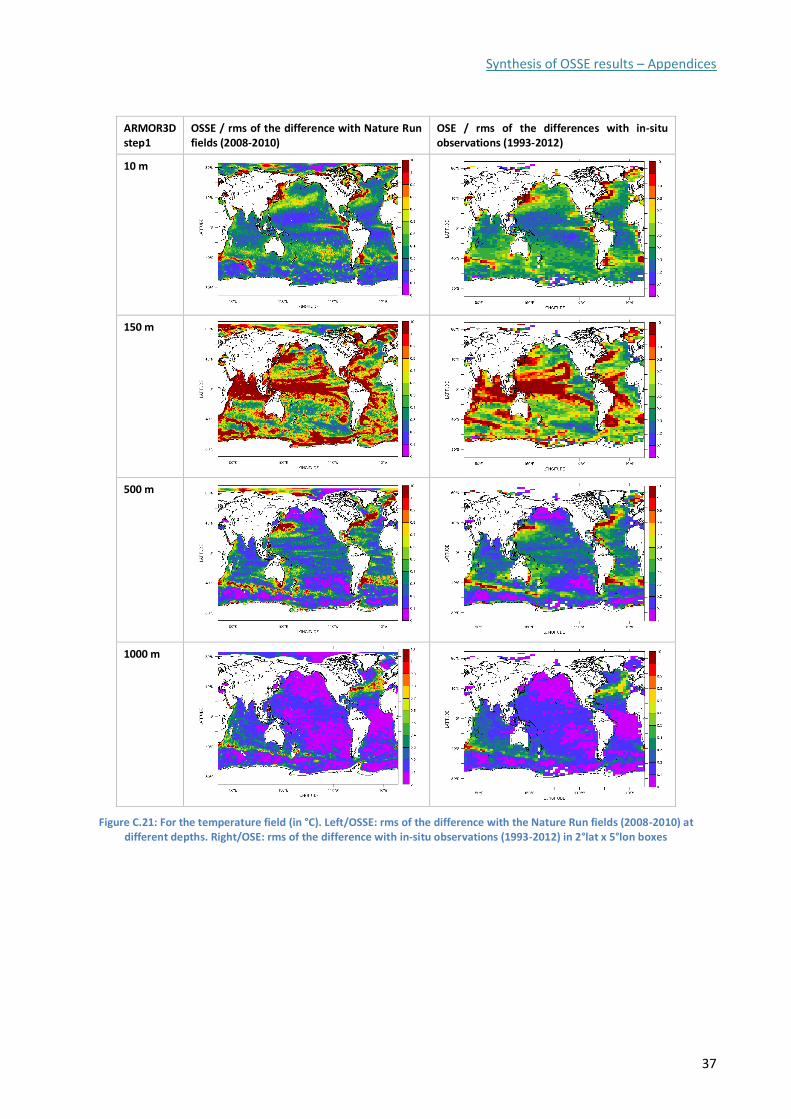
Synthesis of OSSE results – Appendices
37
ARMOR3D step1
OSSE / rms of the difference with Nature Run fields (2008-2010)
OSE / rms of the differences with in-situ observations (1993-2012)
10 m
150 m
500 m
1000 m
Figure C.21: For the temperature field (in °C). Left/OSSE: rms of the difference with the Nature Run fields (2008-2010) at different depths. Right/OSE: rms of the difference with in-situ observations (1993-2012) in 2°lat x 5°lon boxes
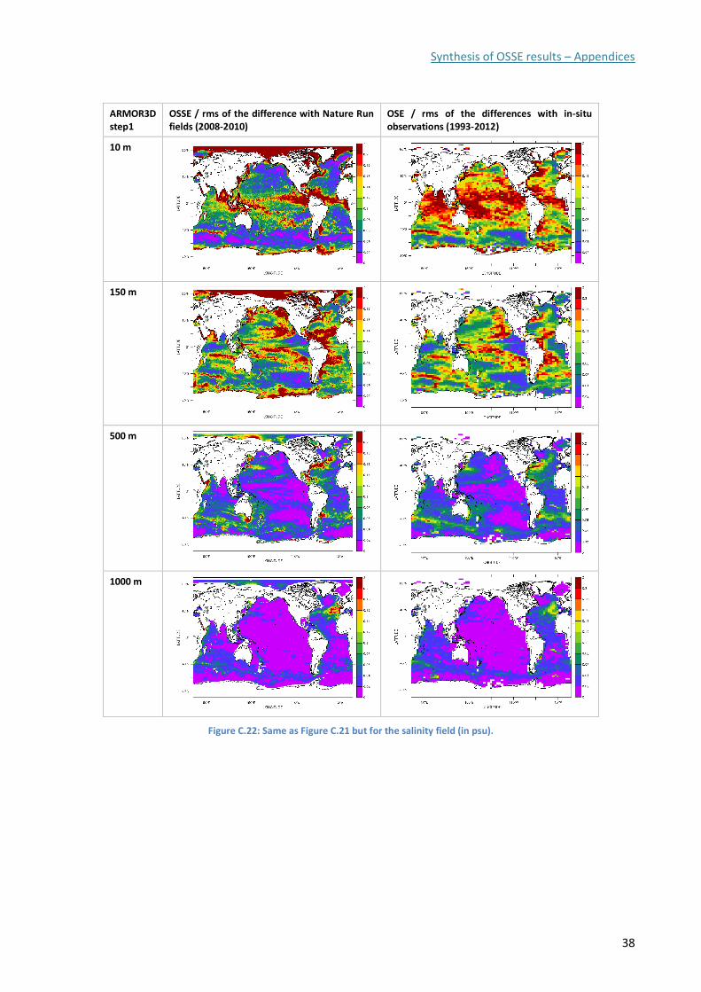
Synthesis of OSSE results – Appendices
38
ARMOR3D step1
OSSE / rms of the difference with Nature Run fields (2008-2010)
OSE / rms of the differences with in-situ observations (1993-2012)
10 m
150 m
500 m
1000 m
Figure C.22: Same as Figure C.21 but for the salinity field (in psu).
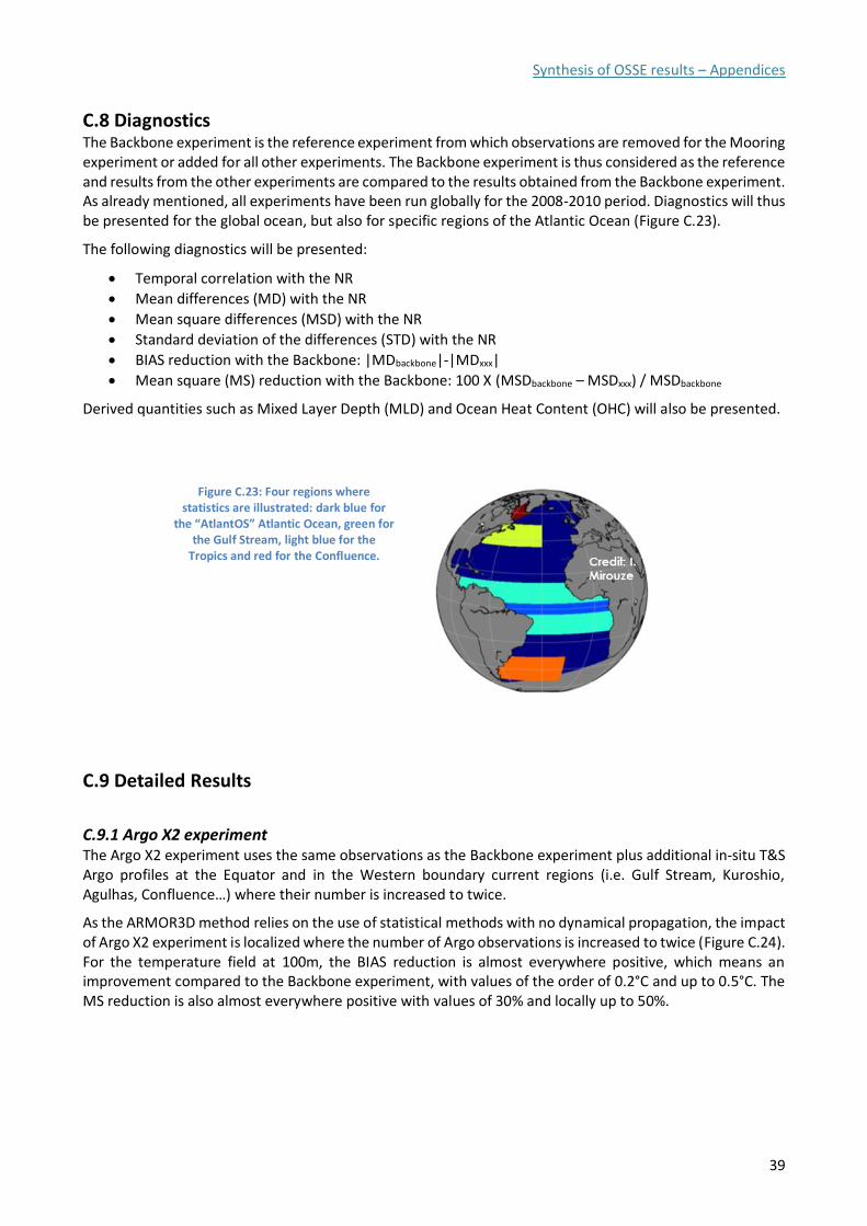
Synthesis of OSSE results – Appendices
39
C.8 Diagnostics The Backbone experiment is the reference experiment from which observations are removed for the Mooring experiment or added for all other experiments. The Backbone experiment is thus considered as the reference and results from the other experiments are compared to the results obtained from the Backbone experiment. As already mentioned, all experiments have been run globally for the 2008-2010 period. Diagnostics will thus be presented for the global ocean, but also for specific regions of the Atlantic Ocean (Figure C.23).
The following diagnostics will be presented:
• Temporal correlation with the NR
• Mean differences (MD) with the NR
• Mean square differences (MSD) with the NR
• Standard deviation of the differences (STD) with the NR
• BIAS reduction with the Backbone: |MDbackbone|-|MDxxx|
• Mean square (MS) reduction with the Backbone: 100 X (MSDbackbone – MSDxxx) / MSDbackbone
Derived quantities such as Mixed Layer Depth (MLD) and Ocean Heat Content (OHC) will also be presented.
Figure C.23: Four regions where statistics are illustrated: dark blue for
the “AtlantOS” Atlantic Ocean, green for the Gulf Stream, light blue for the
Tropics and red for the Confluence.
C.9 Detailed Results
C.9.1 Argo X2 experiment The Argo X2 experiment uses the same observations as the Backbone experiment plus additional in-situ T&S Argo profiles at the Equator and in the Western boundary current regions (i.e. Gulf Stream, Kuroshio, Agulhas, Confluence…) where their number is increased to twice.
As the ARMOR3D method relies on the use of statistical methods with no dynamical propagation, the impact of Argo X2 experiment is localized where the number of Argo observations is increased to twice (Figure C.24). For the temperature field at 100m, the BIAS reduction is almost everywhere positive, which means an improvement compared to the Backbone experiment, with values of the order of 0.2°C and up to 0.5°C. The MS reduction is also almost everywhere positive with values of 30% and locally up to 50%.
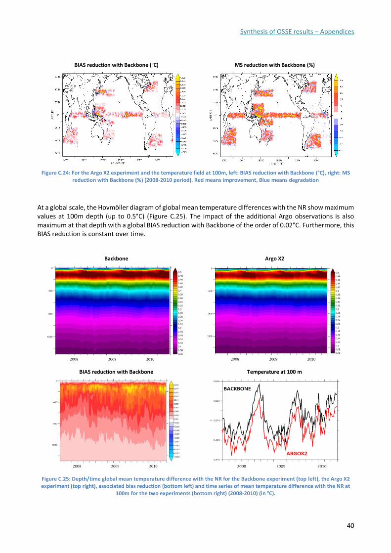
Synthesis of OSSE results – Appendices
40
BIAS reduction with Backbone (°C)
MS reduction with Backbone (%)
Figure C.24: For the Argo X2 experiment and the temperature field at 100m, left: BIAS reduction with Backbone (°C), right: MS reduction with Backbone (%) (2008-2010 period). Red means improvement, Blue means degradation
At a global scale, the Hovmöller diagram of global mean temperature differences with the NR show maximum values at 100m depth (up to 0.5°C) (Figure C.25). The impact of the additional Argo observations is also maximum at that depth with a global BIAS reduction with Backbone of the order of 0.02°C. Furthermore, this BIAS reduction is constant over time.
Backbone
Argo X2
BIAS reduction with Backbone
Temperature at 100 m
Figure C.25: Depth/time global mean temperature difference with the NR for the Backbone experiment (top left), the Argo X2 experiment (top right), associated bias reduction (bottom left) and time series of mean temperature difference with the NR at
100m for the two experiments (bottom right) (2008-2010) (in °C).
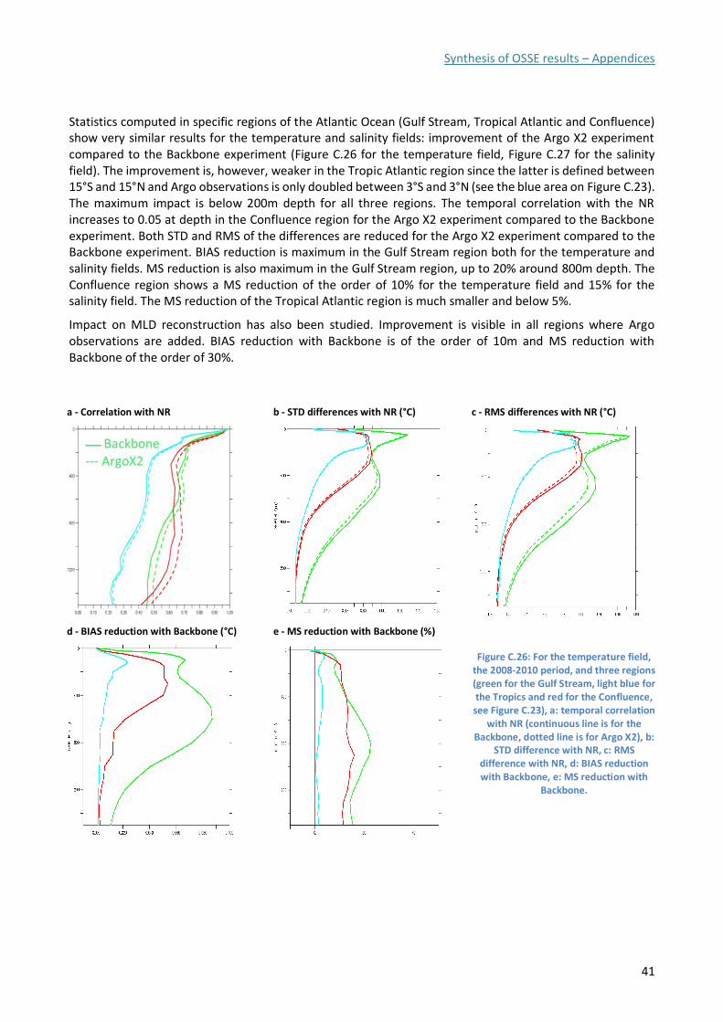
Synthesis of OSSE results – Appendices
41
Statistics computed in specific regions of the Atlantic Ocean (Gulf Stream, Tropical Atlantic and Confluence) show very similar results for the temperature and salinity fields: improvement of the Argo X2 experiment compared to the Backbone experiment (Figure C.26 for the temperature field, Figure C.27 for the salinity field). The improvement is, however, weaker in the Tropic Atlantic region since the latter is defined between 15°S and 15°N and Argo observations is only doubled between 3°S and 3°N (see the blue area on Figure C.23). The maximum impact is below 200m depth for all three regions. The temporal correlation with the NR increases to 0.05 at depth in the Confluence region for the Argo X2 experiment compared to the Backbone experiment. Both STD and RMS of the differences are reduced for the Argo X2 experiment compared to the Backbone experiment. BIAS reduction is maximum in the Gulf Stream region both for the temperature and salinity fields. MS reduction is also maximum in the Gulf Stream region, up to 20% around 800m depth. The Confluence region shows a MS reduction of the order of 10% for the temperature field and 15% for the salinity field. The MS reduction of the Tropical Atlantic region is much smaller and below 5%.
Impact on MLD reconstruction has also been studied. Improvement is visible in all regions where Argo observations are added. BIAS reduction with Backbone is of the order of 10m and MS reduction with Backbone of the order of 30%.
a - Correlation with NR
b - STD differences with NR (°C)
c - RMS differences with NR (°C)
d - BIAS reduction with Backbone (°C)
e - MS reduction with Backbone (%)
Figure C.26: For the temperature field, the 2008-2010 period, and three regions (green for the Gulf Stream, light blue for the Tropics and red for the Confluence, see Figure C.23), a: temporal correlation
with NR (continuous line is for the Backbone, dotted line is for Argo X2), b:
STD difference with NR, c: RMS difference with NR, d: BIAS reduction with Backbone, e: MS reduction with
Backbone.
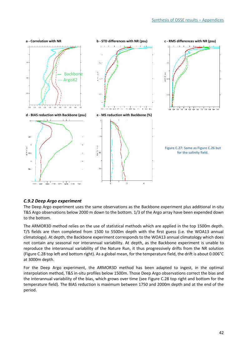
Synthesis of OSSE results – Appendices
42
a - Correlation with NR
b - STD differences with NR (psu)
c - RMS differences with NR (psu)
d - BIAS reduction with Backbone (psu)
e - MS reduction with Backbone (%)
Figure C.27: Same as Figure C.26 but for the salinity field.
C.9.2 Deep Argo experiment The Deep Argo experiment uses the same observations as the Backbone experiment plus additional in-situ T&S Argo observations below 2000 m down to the bottom. 1/3 of the Argo array have been expended down to the bottom.
The ARMOR3D method relies on the use of statistical methods which are applied in the top 1500m depth. T/S fields are then completed from 1500 to 5500m depth with the first guess (i.e. the WOA13 annual climatology). At depth, the Backbone experiment corresponds to the WOA13 annual climatology which does not contain any seasonal nor interannual variability. At depth, as the Backbone experiment is unable to reproduce the interannual variability of the Nature Run, it thus progressively drifts from the NR solution (Figure C.28 top left and bottom right). As a global mean, for the temperature field, the drift is about 0.006°C at 3000m depth.
For the Deep Argo experiment, the ARMOR3D method has been adapted to ingest, in the optimal interpolation method, T&S in-situ profiles below 1500m. Those Deep Argo observations correct the bias and the interannual variability of the bias, which grows over time (see Figure C.28 top right and bottom for the temperature field). The BIAS reduction is maximum between 1750 and 2000m depth and at the end of the period.
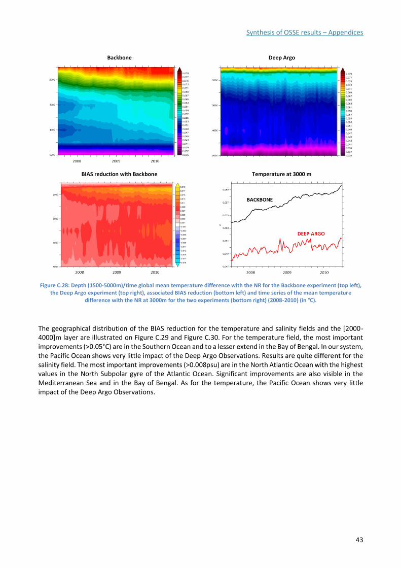
Synthesis of OSSE results – Appendices
43
Backbone
Deep Argo
BIAS reduction with Backbone
Temperature at 3000 m
Figure C.28: Depth (1500-5000m)/time global mean temperature difference with the NR for the Backbone experiment (top left), the Deep Argo experiment (top right), associated BIAS reduction (bottom left) and time series of the mean temperature
difference with the NR at 3000m for the two experiments (bottom right) (2008-2010) (in °C).
The geographical distribution of the BIAS reduction for the temperature and salinity fields and the [2000-4000]m layer are illustrated on Figure C.29 and Figure C.30. For the temperature field, the most important improvements (>0.05°C) are in the Southern Ocean and to a lesser extend in the Bay of Bengal. In our system, the Pacific Ocean shows very little impact of the Deep Argo Observations. Results are quite different for the salinity field. The most important improvements (>0.008psu) are in the North Atlantic Ocean with the highest values in the North Subpolar gyre of the Atlantic Ocean. Significant improvements are also visible in the Mediterranean Sea and in the Bay of Bengal. As for the temperature, the Pacific Ocean shows very little impact of the Deep Argo Observations.
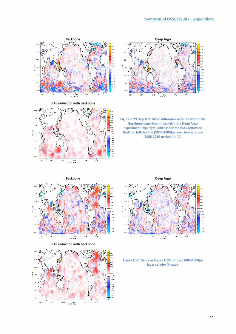
Synthesis of OSSE results – Appendices
44
Backbone
Deep Argo
BIAS reduction with Backbone
Figure C.29: Top left: Mean difference with the NR for the Backbone experiment (top left), the Deep Argo
experiment (top right) and associated BIAS reduction (bottom left) for the [2000-4000]m layer temperature
(2008-2010 period) (in °C).
Backbone
Deep Argo
BIAS reduction with Backbone
Figure C.30: Same as Figure C.29 for the [2000-4000]m layer salinity (in psu).
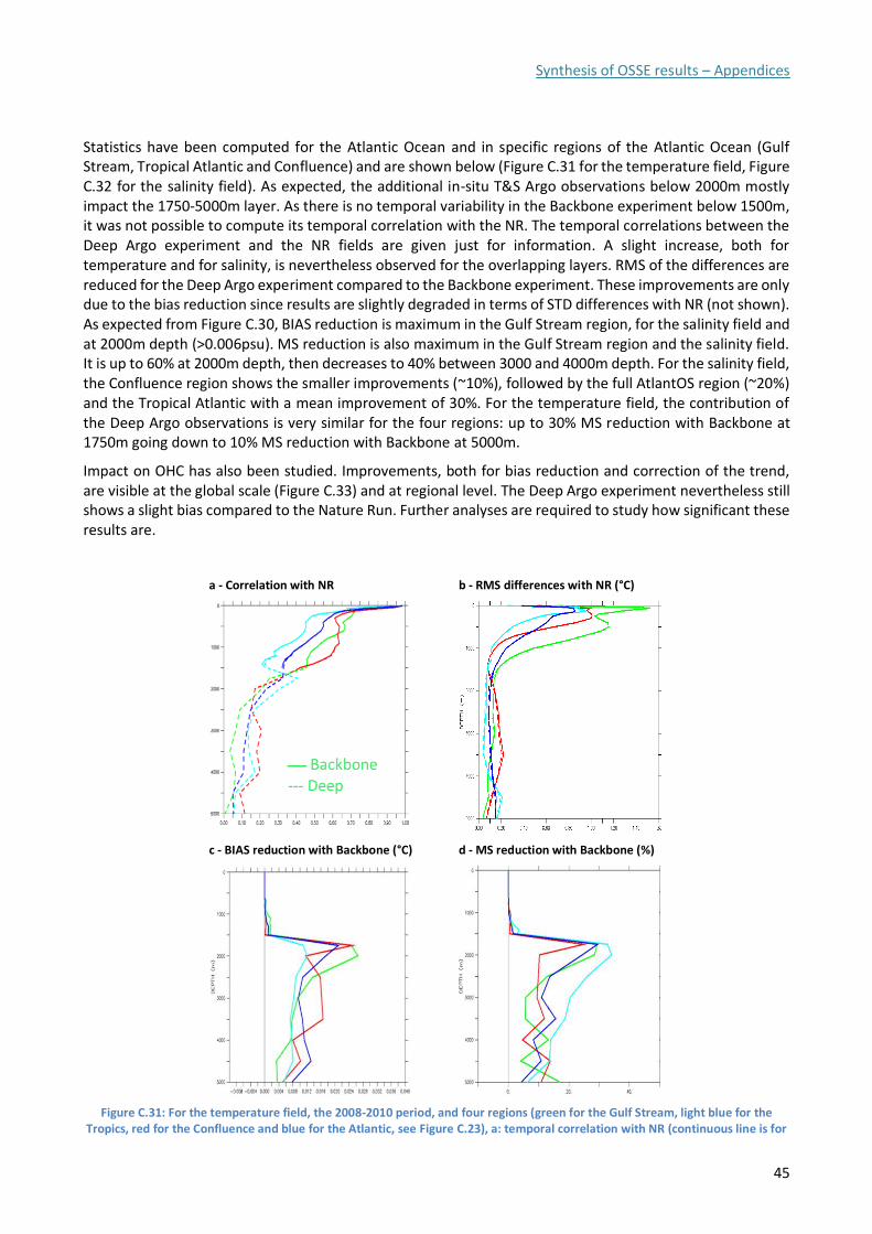
Synthesis of OSSE results – Appendices
45
Statistics have been computed for the Atlantic Ocean and in specific regions of the Atlantic Ocean (Gulf Stream, Tropical Atlantic and Confluence) and are shown below (Figure C.31 for the temperature field, Figure C.32 for the salinity field). As expected, the additional in-situ T&S Argo observations below 2000m mostly impact the 1750-5000m layer. As there is no temporal variability in the Backbone experiment below 1500m, it was not possible to compute its temporal correlation with the NR. The temporal correlations between the Deep Argo experiment and the NR fields are given just for information. A slight increase, both for temperature and for salinity, is nevertheless observed for the overlapping layers. RMS of the differences are reduced for the Deep Argo experiment compared to the Backbone experiment. These improvements are only due to the bias reduction since results are slightly degraded in terms of STD differences with NR (not shown). As expected from Figure C.30, BIAS reduction is maximum in the Gulf Stream region, for the salinity field and at 2000m depth (>0.006psu). MS reduction is also maximum in the Gulf Stream region and the salinity field. It is up to 60% at 2000m depth, then decreases to 40% between 3000 and 4000m depth. For the salinity field, the Confluence region shows the smaller improvements (~10%), followed by the full AtlantOS region (~20%) and the Tropical Atlantic with a mean improvement of 30%. For the temperature field, the contribution of the Deep Argo observations is very similar for the four regions: up to 30% MS reduction with Backbone at 1750m going down to 10% MS reduction with Backbone at 5000m.
Impact on OHC has also been studied. Improvements, both for bias reduction and correction of the trend, are visible at the global scale (Figure C.33) and at regional level. The Deep Argo experiment nevertheless still shows a slight bias compared to the Nature Run. Further analyses are required to study how significant these results are.
a - Correlation with NR
b - RMS differences with NR (°C)
c - BIAS reduction with Backbone (°C)
d - MS reduction with Backbone (%)
Figure C.31: For the temperature field, the 2008-2010 period, and four regions (green for the Gulf Stream, light blue for the Tropics, red for the Confluence and blue for the Atlantic, see Figure C.23), a: temporal correlation with NR (continuous line is for
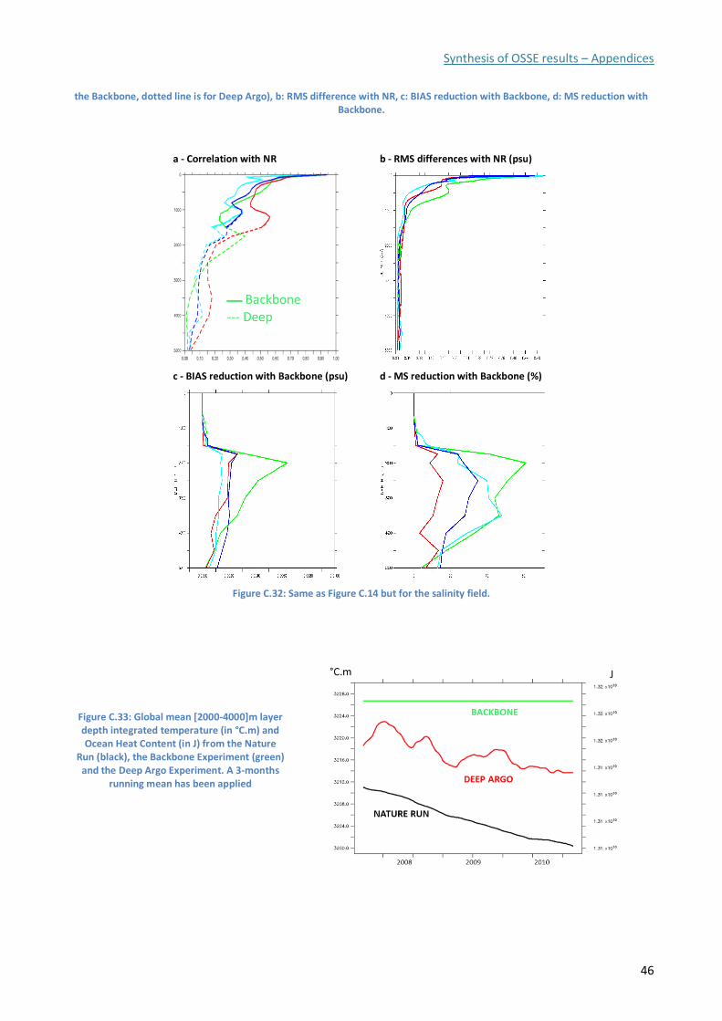
Synthesis of OSSE results – Appendices
46
the Backbone, dotted line is for Deep Argo), b: RMS difference with NR, c: BIAS reduction with Backbone, d: MS reduction with Backbone.
a - Correlation with NR
b - RMS differences with NR (psu)
c - BIAS reduction with Backbone (psu)
d - MS reduction with Backbone (%)
Figure C.32: Same as Figure C.14 but for the salinity field.
Figure C.33: Global mean [2000-4000]m layer depth integrated temperature (in °C.m) and Ocean Heat Content (in J) from the Nature
Run (black), the Backbone Experiment (green) and the Deep Argo Experiment. A 3-months
running mean has been applied
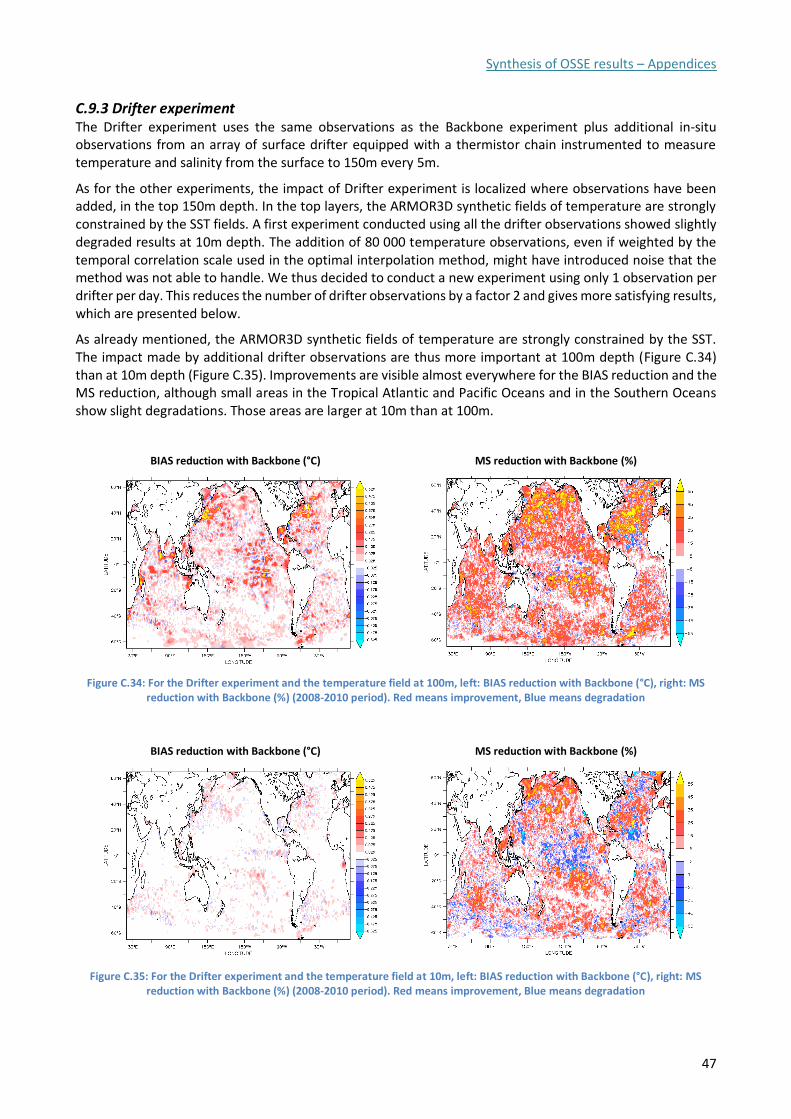
Synthesis of OSSE results – Appendices
47
C.9.3 Drifter experiment The Drifter experiment uses the same observations as the Backbone experiment plus additional in-situ observations from an array of surface drifter equipped with a thermistor chain instrumented to measure temperature and salinity from the surface to 150m every 5m.
As for the other experiments, the impact of Drifter experiment is localized where observations have been added, in the top 150m depth. In the top layers, the ARMOR3D synthetic fields of temperature are strongly constrained by the SST fields. A first experiment conducted using all the drifter observations showed slightly degraded results at 10m depth. The addition of 80 000 temperature observations, even if weighted by the temporal correlation scale used in the optimal interpolation method, might have introduced noise that the method was not able to handle. We thus decided to conduct a new experiment using only 1 observation per drifter per day. This reduces the number of drifter observations by a factor 2 and gives more satisfying results, which are presented below.
As already mentioned, the ARMOR3D synthetic fields of temperature are strongly constrained by the SST. The impact made by additional drifter observations are thus more important at 100m depth (Figure C.34) than at 10m depth (Figure C.35). Improvements are visible almost everywhere for the BIAS reduction and the MS reduction, although small areas in the Tropical Atlantic and Pacific Oceans and in the Southern Oceans show slight degradations. Those areas are larger at 10m than at 100m.
BIAS reduction with Backbone (°C)
MS reduction with Backbone (%)
Figure C.34: For the Drifter experiment and the temperature field at 100m, left: BIAS reduction with Backbone (°C), right: MS reduction with Backbone (%) (2008-2010 period). Red means improvement, Blue means degradation
BIAS reduction with Backbone (°C)
MS reduction with Backbone (%)
Figure C.35: For the Drifter experiment and the temperature field at 10m, left: BIAS reduction with Backbone (°C), right: MS reduction with Backbone (%) (2008-2010 period). Red means improvement, Blue means degradation
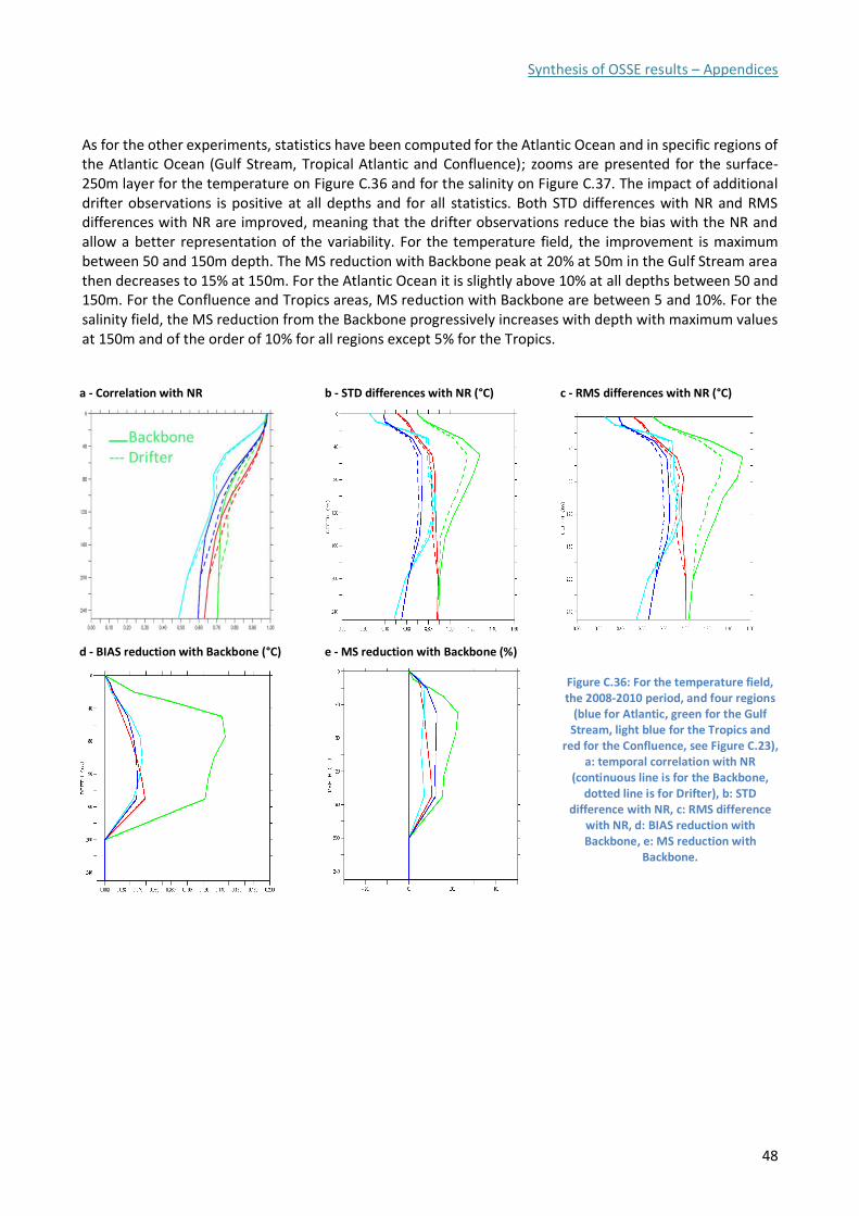
Synthesis of OSSE results – Appendices
48
As for the other experiments, statistics have been computed for the Atlantic Ocean and in specific regions of the Atlantic Ocean (Gulf Stream, Tropical Atlantic and Confluence); zooms are presented for the surface-250m layer for the temperature on Figure C.36 and for the salinity on Figure C.37. The impact of additional drifter observations is positive at all depths and for all statistics. Both STD differences with NR and RMS differences with NR are improved, meaning that the drifter observations reduce the bias with the NR and allow a better representation of the variability. For the temperature field, the improvement is maximum between 50 and 150m depth. The MS reduction with Backbone peak at 20% at 50m in the Gulf Stream area then decreases to 15% at 150m. For the Atlantic Ocean it is slightly above 10% at all depths between 50 and 150m. For the Confluence and Tropics areas, MS reduction with Backbone are between 5 and 10%. For the salinity field, the MS reduction from the Backbone progressively increases with depth with maximum values at 150m and of the order of 10% for all regions except 5% for the Tropics.
a - Correlation with NR
b - STD differences with NR (°C)
c - RMS differences with NR (°C)
d - BIAS reduction with Backbone (°C)
e - MS reduction with Backbone (%)
Figure C.36: For the temperature field, the 2008-2010 period, and four regions
(blue for Atlantic, green for the Gulf Stream, light blue for the Tropics and
red for the Confluence, see Figure C.23), a: temporal correlation with NR
(continuous line is for the Backbone, dotted line is for Drifter), b: STD
difference with NR, c: RMS difference with NR, d: BIAS reduction with Backbone, e: MS reduction with
Backbone.
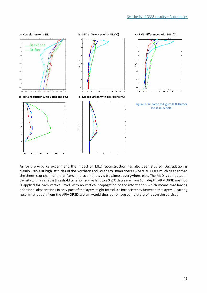
Synthesis of OSSE results – Appendices
49
a - Correlation with NR
b - STD differences with NR (°C)
c - RMS differences with NR (°C)
d - BIAS reduction with Backbone (°C)
e - MS reduction with Backbone (%)
Figure C.37: Same as Figure C.36 but for the salinity field.
As for the Argo X2 experiment, the impact on MLD reconstruction has also been studied. Degradation is clearly visible at high latitudes of the Northern and Southern Hemispheres where MLD are much deeper than the thermistor chain of the drifters. Improvement is visible almost everywhere else. The MLD is computed in density with a variable threshold criterion equivalent to a 0.2°C decrease from 10m depth. ARMOR3D method is applied for each vertical level, with no vertical propagation of the information which means that having additional observations in only part of the layers might introduce inconsistency between the layers. A strong recommendation from the ARMOR3D system would thus be to have complete profiles on the vertical.
Synthesis of OSSE results – Appendices
50
C.9.4 Mooring experiment The mooring experiment uses the same observations as the Backbone experiment less the moorings. Unlike other experiments, observations are removed here and not added.
As for the other experiments, the impact of Mooring experiment is localized where observations have been removed, very locally at each mooring site. Results show a degradation compared to the Backbone experiment, up to -50% MS error reduction with the Backbone experiment at each mooring site. Those results have not been examined further. In fact, as the ARMOR3D method relies on the use of statistical methods, with no dynamical propagation, neither in space nor in time, the method might not be appropriate to analyze the impact of a very localized observing system.
C.10 Conclusions
As the ARMOR3D method relies on the use of statistical methods with no dynamical propagation, neither in space (horizontal & vertical) nor in time, the impact of additional or less observations are localized where observations have been added or removed. This is on one side a strength of the method since it directly and rapidly react to any change in the observing system, but on the other hand a limitation. The lack of vertical propagation for short profiles like the ones provided by the Drifter array equipped with a thermistor chain might introduce inconsistency between the layers. The lack of temporal propagation means that the system does not keep the memory of previous analyzes but starts from the same first guess at each date. This could cause jumps into the solution if in-situ observations are not regularly available, particularly for the deep layers. A strong recommendation from the ARMOR3D system would thus be to have complete profiles on the vertical, and regularly available in time.
Results from the present study show that there is a better representation of the variability with the additional observations provided that the areas where the Argo observing system is doubled (Argo X2 experiment) and where drifter equipped with a thermistor chain instrumented from the surface to 150m are available (Drifter experiment). Moreover, results show that the Deep Argo observing system complete well the current observing system by correcting the bias that exist at depth and their interannual variability.
C.11 References
Gasparin et al., 2018a: Synthesis of the Physical OSSE results, Report D1.5 of the AtlantOS project.
Gasparin et al., 2018b: A large-scale view of oceanic variability from 2007 to 2015 in the global high-resolution monitoring and forecasting system at Mercator Océan, In revision in Journal of Marine Systems
Guinehut S., A.-L. Dhomps, G. Larnicol and P.-Y. Le Traon, 2012: High resolution 3D temperature and salinity fields derived from in situ and satellite observations. Ocean Sci., 8, 845-857, doi:10.5194/os-8-845-2012.
Halliwell, G. R., A. Srinivasan, V. Kourafalou, H. Yang, D. Willey, M. Le Hénaff, and R. Atlas, 2014: Rigorous evaluation of a fraternal twin ocean OSSE system for the open Gulf of Mexico. Journal of Atmospheric and Oceanic Technology, 31 (1), 105–130.
Oke, P. R., Larnicol, G., Fujii, Y., Smith, G. C., Lea, D. J., Guinehut, S., Rémy, E., Alonso Balmaseda, M., Rykova, T., Surcel- Colan, D., Martin, M. J., Sellar, A. A., Mulet, S., and Turpin, V.: Assessing the impact of observations on ocean forecasts and re- analyses: Part 1, Global studies, J. Oper. Oceanogr., 8, s49–s62, https://doi.org/10.1080/1755876X.2015.1022067, 2015.