Erik P. GilsonPrinceton Plasma Physics Laboratory

9th International Workshop on Nonneutral Plasmas Columbia University

June 17th, 2008

*This work is supported by the U.S. Department of Energy.

Overview ofIntense Beam Simulation Experiments

Performed Using thePaul Trap Simulator Experiment (PTSX)*

In collaboration with:

Andy Carpe, Moses Chung, Ronald C. Davidson, Mikhail Dorf, Philip Efthimion, Andrew Godbehere, Richard Majeski, Hong Qin, Edward Startsev, Hua Wang

• Purpose: PTSX simulates, in a compact experiment, the transverse nonlinear dynamics of intense beam propagation over large distances through magnetic alternating-gradient transport systems.

• Applications: Accelerator systems for high energy and nuclear physics applications, heavy ion fusion, spallation neutron sources, and high energy density physics.

PTSX Simulates Nonlinear Beam Dynamicsin Magnetic Alternating-Gradient Systems

Other Intense-Beam Studies, Paul-trap-based and otherwise:

Okamoto and Tanaka

Drewsen et al.

Kishek et al.

Scientific Motivation

• Beam mismatch and envelope instabilities;

• Collective wave excitations;

• Chaotic particle dynamics and production of halo particles;

• Mechanisms for emittance growth;

• Compression techniques; and

• Effects of distribution function on stability properties.

As self-field effects become important, it is important to develop an understanding of:

( ) ( ) ( )( ) ( ) ( )yxqfoc

yxqfoc

q

yxz

xyzB

eexF

eexBˆˆ

ˆˆ

−−=

+′=

κ

2

)()(

cmzBZe

z qq βγ

κ′

≡

Magnetic Alternating-Gradient Transport Systems

SS

N

S

xz

y

Transverse Focusing Frequency andPhase Advance Characterize the Motion

In one lattice period, S, the smooth trajectory’s vacuum phase advance, σv, is 35 degrees.

Transverse focusing frequency, ωq

σv must be less than 180 for bounded orbits.

Space-charge decreases σv to σ.

2 m

0.4 m ))((21),,( 22 yxttyxe qap −′= κφ

20

)(8)(

wq rm

teVtπ

κ =′

0.2 m

PTSX Configuration – A Cylindrical Paul Trap

5x10-9 TorrPressure133 amuCesium ion mass105-106 cm-3Density< 10 VIon source grid voltages

< 100 kHz< 150 V~ 400 V

FrequencyEnd electrode voltageMaximum wall voltage

~ 1 cmPlasma radius10 cmWall radius2 mPlasma length

ξπ

ωf rm

eV

wq 2

max 08=

sinusoidal in this work

22

1π

ξ =

3423 ηη

ξ−

=

for a sinusoidal waveform V(t).

for a periodic step function waveform V(t) with fill factor η.

Pure Ion Plasma

0 max2

qsfv

Vf fω

σ = ∝

Transverse Dynamics are the Same Including Self-Field Effects

))((21),,( 22 yxttyxe qap −′= κφ

20

)(8)(

wq rm

teVtπ

κ =′

( ) ( ) ( )yxqfoc

q xyzB eexB ˆˆ +′=

( ) ( ) ( )yxqfoc yxz eexF ˆˆ −−= κ

2

)()(

cmzBZe

z qq βγ

κ′

=

[ ]),,(),,(22 syxAsyxcm

Zezβφ

βγψ −=

( ) ( ) 0=⎭⎬⎫

⎩⎨⎧

′∂∂

⎟⎟⎠

⎞⎜⎜⎝

⎛∂∂

+−−′∂

∂⎟⎠⎞

⎜⎝⎛

∂∂

+−∂∂′+

∂∂′+

∂∂

bqq fyy

ysxx

xsy

yx

xs

ψκψκ

∫ ′′−=⎟⎟⎠

⎞⎜⎜⎝

⎛∂∂

+∂∂

bfydxdN

Kyx

πψ 22

2

2

2

Quadrupolar Focusing

Self-Forces usual φself(x,y,t)

Field Equations Poisson’s Equation

Vlasov Equation

Transverse Dynamics are the Same Including Self-Field Effects

•Long coasting beams

•Beam radius << lattice period

•Motion in beam frame is nonrelativistic

Ions in PTSX have the same transverse equations of motion as ions in an alternating-gradient system in the beam frame.

If…

Then, when in the beam frame, both systems have…

•Quadrupolar external forces

•Self-forces governed by a Poisson-like equation

•Distributions evolve according to nonlinear Vlasov-Maxwell equation

Smooth-Focusing Equilibria areParameterized by s

( ) ( ) ( )⎥⎥⎦

⎤

⎢⎢⎣

⎡ +−=

kTrqrm

nrns

q

22

exp022 φω

( )0

1 s qn rr

r r rφ

ε∂ ∂

=∂ ∂

In thermal equilibrium,

Poisson’s equation becomes a nonlinear equation for φs that must be solved numerically.

s = 0…0.9

s = 0.99

s = 0.9999 s = 1

)()0( 2 sRnN ζπ=

ζ(s) is determined numerically.ζ(0) = 1ζ(1) = 2 0 0.1 0.2 0.3 0.4 0.5 0.6 0.7 0.8 0.9 1

1

1.1

1.2

1.3

1.4

1.5

1.6

1.7

1.8

1.9

2

ξ

s

2

2

(0)1

2p

q

sωω

≡ <

Normalized intensity parameter s.

s ~ 0.2 for SNS and Tevatron injector.

s ~ 0.99 for HIF

Global Force Balance

22 2 2

4qo

Nqm R kTωπε

= +

If p = n kT, then the statement of local force balance on a fluid element can be manipulated to give a global force balance equation.

2p qF mn rω= −

pressureF kT n= − ∇EF nqE=

2 2

0q

nr dr mn r qnE kTr

ω∞ ∂⎛ ⎞= −⎜ ⎟∂⎝ ⎠∫

2q

nmn r qnE kTr

ω ∂= −

∂Fluid Element

where R is the root-mean-squared radius and N is the line charge.

Note that N and R are measured by integrating the experimentally obtained density profiles n(r).

kT is inferred from this global force balance.

1.25 in

Electrodes, Ion Source, and Collector

5 mm

Broad flexibility in applying V(t) to electrodes with arbitrary function generator.

Increasing source current creates plasmas with intense space-charge.

Large dynamic range using sensitive electrometer.

Measures average Q(r).

• s = ωp2/2ωq

2

= 0.18.

• V0 = 235 V f = 75 kHz σv = 49o

• At f = 75 kHz, a lifetime of 100 ms corresponds to 7,500 lattice periods.

• If S is 1 m, the PTSX simulation experiment would correspond to a 7.5 km beamline.

PTSX Simulates Equivalent PropagationDistances of 7.5 km

0.00E+00

5.00E-03

1.00E-02

1.50E-02

2.00E-02

2.50E-02

0 50 100 150 200 250 3000 50 100 150 200 250 300

1

0

2

r

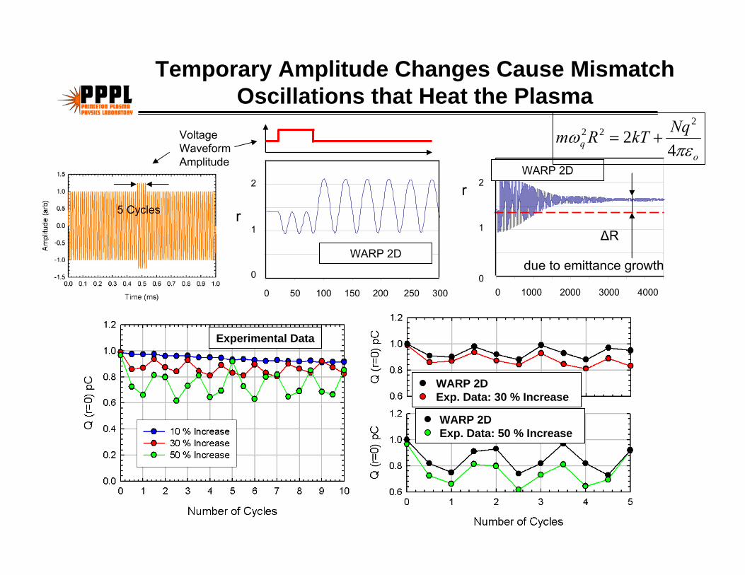
Temporary Amplitude Changes Cause Mismatch Oscillations that Heat the Plasma

0.00E+00

5.00E-03

1.00E-02

1.50E-02

2.00E-02

2.50E-02

0 500 1000 1500 2000 2500 3000 3500 4000 4500

r

ΔR

due to emittance growth

0 1000 2000 3000 4000

1

0

2

Voltage Waveform Amplitude

WARP 2D

WARP 2D

WARP 2DExp. Data: 30 % Increase

WARP 2DExp. Data: 50 % Increase

Experimental Data

oq

NqkTRmπε

ω4

22

22 +=

5 Cycles

Transverse Bunch Compression by Increasing ωq

oq

NqkTRmπε

ω4

22

22 +=

If line density N is constant and kT doesn’t change too much, then increasing ωq decreases R, and the bunch is compressed.

ξπ

ωf rm

eV

wq 2

max 08=

Either1.) increasing V0 max (increasing magnetic field strength) or 2.) decreasing f (increasing the magnet spacing)increases ωq

ωq 1.5 ωq

Compression is Possible but Increasing Phase Advance Degrades Transverse Confinement

s = 0.08, kT = 1.6 eV

s = 0.14, kT = 1.4 eV

s = 0.02, kT = 4.7 eV

ωq 1.5 ωq

σv = 50o 60%

σv = 75o 40%

σv = 112o 450%

N ~ constant Emittance increases

oq

NqkTRmπε

ω4

22

22 += 0 maxq

Vf

ω ∝ 0 max2

sfv

Vf

σ ∝

Adiabatic Amplitude Increases Transversely Compress the Bunch Better

R = 0.79 cmkT = 0.16 eVs = 0.18Δε = 10%

InstantaneousR = 0.93 cmkT = 0.58 eVs = 0.08Δε = 140%

AdiabaticR = 0.63 cmkT = 0.26 eVs = 0.10Δε = 10%

• s = ωp2/2ωq

2 = 0.20 • ν/ν0 = 0.88 • V0 max = 150 V • f = 60 kHz • σv = 49o

20% increase in V0 max 90% increase in V0 max

σv = 63o σv = 111o

ε ~R√ kT

BaselineR = 0.83 cmkT = 0.12 eVs = 0.20

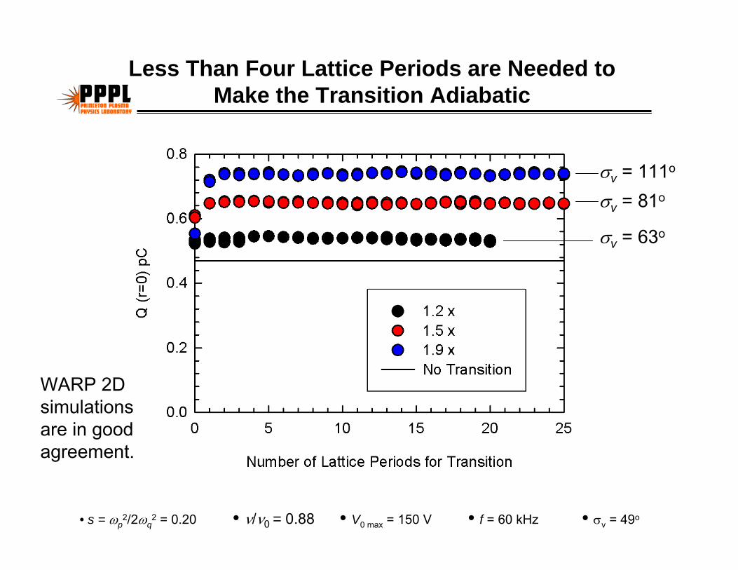
Less Than Four Lattice Periods are Needed to Make the Transition Adiabatic

σv = 63o

σv = 111o

σv = 81o

• s = ωp2/2ωq

2 = 0.20 • ν/ν0 = 0.88 • V0 max = 150 V • f = 60 kHz • σv = 49o

WARP 2D simulations are in good agreement.

Time (ms)

0.0 0.2 0.4 0.6 0.8 1.0

phas

e (r

ad)

0

50

100

150

200

Time (ms)

0.0 0.2 0.4 0.6 0.8 1.0

phas

e (r

ad)

0

50

100

150

200

250

300

Time (ms)

0.0 0.2 0.4 0.6 0.8 1.0

kHz

-150

-100

-50

0

50

100

Time (ms)

0.0 0.2 0.4 0.6 0.8 1.0

Am

plitu

de (a

rb)

-1.5

-1.0

-0.5

0.0

0.5

1.0

1.5

Time (ms)

0.0 0.2 0.4 0.6 0.8 1.0

Am

plitu

de (a

rb)

-1.5

-1.0

-0.5

0.0

0.5

1.0

1.5

( )⎥⎦

⎤⎢⎣

⎡+

−−−+= 1

2tanh

22)( 21

τπφ tt

tff

tft fif

( )0

21

2coshln

422)( f

ttfft

fft iffi −⎥⎦

⎤⎢⎣

⎡ −−−+

+=

ττ

πφ

πφ2

)(t

πφ2

)(t

( ) ( )tVtV φsinmax 0=

Increasing ωq by Adiabatically Decreasing f

( ) ( )tVtV φsinmax 0=ξ

πω

f rmeV

wq 2

max 08=

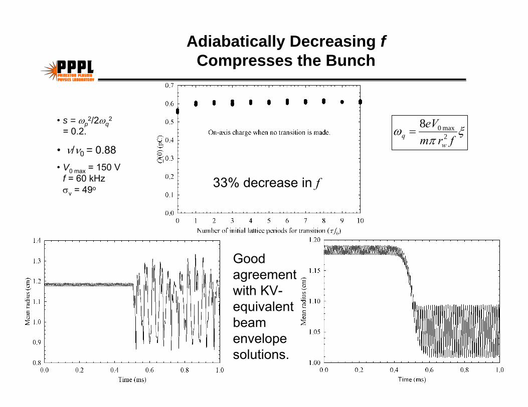
Adiabatically Decreasing fCompresses the Bunch

33% decrease in f

Good agreement with KV-equivalent beam envelope solutions.

ξπ

ωf rm

eV

wq 2

max 08=

• s = ωp2/2ωq

2

= 0.2.

• ν/ν0 = 0.88• V0 max = 150 V

f = 60 kHz σv = 49o

Transverse Confinement is Lost When Single-Particle Orbits are Unstable

τc

2

1qsfv f f

ωσ = ∝

τ = τc

( )⎥⎦

⎤⎢⎣

⎡+

−−−+= 1

2tanh

22)( 21

τπφ tt

tff

tft fif

πφ2

)(t

Measured τc (dots)Set σv max = 180o and solve for τc (line)

τ cf 0

f1 (kHz)

f0 = 60 kHzf0 = 60 kHz

Good Agreement Between Data and KV-Equivalent Beam Envelope Solutions

τc

τf0 = 0

τf0 = 19.9

τ = τc

τf0 = 26

f0 = 60 kHz

Spectrum of measured signal

Quadrupole mode

Breathing mode

ℓ = 2 surface-wave quadrupole mode

ℓ = 0 body-wave breathing mode

( )1 24 3q sω ω= −

( )1 24 2q sω ω= −

Measuring Beam Oscillations and Inferring Beam “Normalized Intensity” s

Segmented collective-mode capacitive pick-up diagnostic is sensitive to beam collective-mode oscillations.

Measured frequencies…

… determine unique “normalized intensity.”

Other modes?

• PTSX is a versatile research facility in which to simulate collective processes and the transverse dynamics of intense charged particle beam propagation over large distances through an alternating-gradient magnetic quadrupole focusing system using a compact laboratory Paul trap.

• PTSX explores important beam physics issues such as:

•Beam mismatch and envelope instabilities;

•Collective wave excitations;

•Chaotic particle dynamics and production of halo particles;

•Mechanisms for emittance growth;

•Compression techniques; and

•Effects of distribution function on stability properties.

PTSX is a Compact Experiment for Studying the Propagation of Beams Over Large Distances