P1.7 Observing Systems Simulation Experiments at NCEP

OSSEs for realistic adaptive targeted DWL

Uniform observation and AIRS

Jack Woollen1+, Michiko Masutani1#, Haibing Sun3%, Yucheng Song1*, Dave Emmitt2, Zoltan Toth1

Steve Lord1, Yuanfu Xie4,

1NOAA/NWS/NCEP/EMC, Camp Springs, MD 2Simpson Weather Associates (SWA), Charlottesville, VA

3NOAA/NESDIS/STAR, Camp Springs, MD 4NOAA/Earth System Research Laboratory, Boulder, CO

#RS Information Systems (RSIS), VA +Science Applications International Corporation (SAIC)

%QSS Group, Inc. *I. M. Systems Group, Inc. (IMSG)

1. Introduction Observing System Simulation Experiments (OSSE) provide a unique methodology for obtaining quantitative evaluation useful in designing advanced meteorological observing systems. The procedure is based on a simulated atmosphere derived from a high resolution state of the art numerical weather prediction model which is run for a rather long period (i.e., a month or more). This is called the Nature Run (NR). Idealized observations are synthesized from the simulated nature to resemble observations found in the real world. Imaginary observations from prospective instruments can also be synthesized and then used in assimilation/forecast experiments to gauge the potential impact of such instruments, if they were to be developed.

The OSSE as performed at the National Centers for Environmental Prediction (NCEP) is the well defined OSSE described in Arnold and Dey (1986). A NR which serves as the truth for the OSSE was generated by the European Center for Medium-range Weather Forecasts (ECMWF) (Becker et al. 1996) and the NCEP Data Assimilation System (DAS) was used to assimilate data. NWP models at NCEP and ECMWF have contrasting physics parameterizations and different algorithms for dynamics and this difference is expected to mimic model error (the difference between an NWP model and the real world) in real world data assimilation.

OSSEs that are conducted at NCEP, in

collaboration with the National Environmental Satellite Data and Information Service (NESDIS), Simpson Weather Associates (SWA), and the National Aeronautics and Space Administration (NASA), in order to evaluate DWL are presented. Throughout the simulation experiments, realistic data were processed. NCEP’s OSSE is the first OSSE where satellite level-1B radiance data were simulated and assimilated. In the OSSE described in Stoffelen et al. (2006), satellite radiance data were simulated (Becker et al. 1996) but not used in OSSEs. In order to avoid misleading results, only data impacts over the Northern Hemisphere were presented by Stoffelen et al. Without radiance data, a large impact from DWL over the Southern Hemisphere (SH) was obtained but does not represent the real world impact. DWL is often simulated as vector wind but was simulated and assimilated as line of sight wind (LOS) in the NCEP OSSE.

The details of NCEP OSSE are described in (Masutani et al 2006). In this paper the further results, which were not included there, are presented. OSSEs for realistic targeted DWL experiments, uniform observations with various resolutions, and a summary of AIRS OSSEs are also presented. 2. OSSE system The NCEP global DAS based on the Spectral Statistical Interpolation (SSI) is used in this paper. SSI is a three-dimensional variational analysis (3D-VAR) scheme and described in Parrish and Derber (1992) and Derber and Wu, 1998). Satellite level-1B radiance data are directly assimilated (McNally et al. 2000). LOS

Corresponding author address:. Michiko Masutani, NOAA/NWS/NCEP/EMC, 5200 Auth Road Rm 207, Camp Springs, MD 20746 Michiko.masutani@noaa.gov

AMS preprint, Symposium on Recent Developments in Atmospheric Applications of Radar and Lidar, New Orleans, LA, 20-24 January 2008

1

winds from DWL are directly used. Spring 2004 versions of NCEP’s operational Medium Range Forecast (MRF) model and DAS were used for data impact tests presented in this paper. Sometimes the inclusion of new instruments requires a major revision to the DAS in order to accommodate both large amounts of data and the increased spectral resolution of the new sounding instruments. More details about the forecast model, SSI and the upgrades are described in Global Climate and Weather Modeling Branch publications (2003, 2004). 3. Adaitive targetted DWL 3.1 Objective In the NCEP OSSE, instead of evaluating a specific instrument, four representative types of DWL are evaluated. Masutani et al (2006) showed evaluated advantage of scanning in DWL and upper level data become more important even in lower levels after a few days forecasts. However, overwhelming technical difficulty in scanning and sufficient power to operate direct detection DWL, which allow measurement at upper levels, in 100% duty cycle become problems. 10% duty cycle with 10 minutes duration is proposed as a possible option but it is hard to warm up the instruments after 90 minutes. On the other hand, coherent DWL, which gives lower altitude data, can be operated 100% duty cycle. If both are used together coherent DWL will keep the instrument warm while providing lower level observations. In this section we are evaluating the best strategies to select 10% of upper level observations. 3.2 Method Three types of lidars are used in the experiments in this section.

● DWL-Upper: An instrument that provides mid- and upper- tropospheric winds only down to the levels of significant cloud coverage. This operate typically only 10% (possibly up to 20%) of the time ● DWL-Lower: An instrument that provides only wind observations from clouds and the PBL. Operates 100% of the time and keeps the instruments warm. ● DWL-NonScan: DWL covers all levels without scanning. This is to mimic the lidar planned for the ADM mission (Stofflen et al. 2005)

In the adaptive targeted DWL experiment, roughly 10% of the observations in each orbit are thus identified to be assimilated, with the maximum error located in the center of the 10% segment with 10 min duration. Forecast results from the adaptive targeting

were compared with five non-adaptive DWL samplings, (Fig.1)

50%(regular): 50% sampling. Each sampling last 10min. 10% (regular): 10% sampling. Each sampling last 10min. 10%(NH Ocean): 10% sampling from NH Ocean. 10% (Tropics):10% sampling from tropics 10% (NH Band): 10% sampling from NH Band including both ocean and land. 0% of DWL-upper

Non scan lidar is also tested to study combined impact with DWL-Lower. The targeting is selected in an idealized manner. Since it is based on the difference between NR (truth) and forecast, targeting assumes knowledge of observation. In order to make this clear, we call this "A perfect 10% adaptive targeted DWL". It is very interesting to note that targeted regions correspond well with NH jet stream and wind from North pole. (Fig. 2) 3.3 Results The data impact is presented as the zonal wave numbers 10-20 component of anomaly correlation (AC) of meridional wind (V) at 200hPa. In Masutani et al (2006), we showed that the improvement in AC forecast skill for the wind fields is about 1-3% even with the scan_DWL, but the data impact shown at all wave numbers is mainly from planetary scale waves. It is expected tthe main impact of DWL would be at smaller scales (Stoffelen et al. 2006). Masutani et al (2006) confirms that the impact is much larger at the synoptic scale with zonal wave numbers 10-20. The improvement in AC is nearly 8%, especially at the 48-72 hour forecast range. Fig 3 shows combined impact of 100% sampling of DWL-Lower and various scenarios of DWL-upper. The results showed that 10% DWL without targeting does not produce much impact (requires at least 50% of the data). A perfect 10% adaptive targeted DWL had 3 day forecast skill similar to the 50% DWL experiment Fixed area targeting did not show better impact than uniform sampling. 10% targeted DWL improves the low level wind forecast after 48 hrs. Combined impact of DWL-NonScan with DWL-Lower is also evaluated in Fig 4. Improvement in AC from experiments without lidar are presented. At 200hPa there are almost no observations by DWL-lower but there is a significant amount of observation by the DWL-NonScan, but with scanning DWL-Lower showing more impact than DWL-NonScan. The combining DWL-NonScan and DWL-Lower, AC will increase 0.3% in analysis and nearly 0.8% in two days forecast. 4. OSSE with Uniform observation The balance between data density and model resolution is investigated using globally uniformly

2

distributed observations. Uniform observation are simulated at 40 levels and with horizontally uniformly-spaced data with mean separation of 1000km, 500km, 200km, are tested. The Fibonacci Grid (Swinbank and Purser 2006) is use to provide uniform data coverage. The results showed that the number of vertical resolution levels is very critical for a high resolution data set. Although high density observations definitely help to improve analysis, forecast skill does not necessarily improve. Particularly, temperature fields suffer more from high density observations. Fig 5 shows 1000km observations produce similar skill to control data. Fig. 6 shows that 500km data improve analysis with T62L28 (Horizontal resolution T62 with 28 vertical levels) but temperature forecast deteriorate after two days. With T170L42 model 500km data is better than 1000km data but 200km data produce worse forecasts after two days (Fig. 6). Fig.5 and Fig 6 show either increasing number of vertical level to 64 or increasing horizontal resolution fix the problem of deterioration of forecast with 500km resolution observations. Once analysis is done with a high resolution model, switching to T62L28 model in forecast does deteriorate the forecasts although the forecast skill reduced. This experiments showed that OSSE will be a very useful tool to prepare the DA system for new instruments. The results showed that without a sufficient number of vertical levels, or sufficient horizontal resolution, a high density of observations could be damaging to the forecast skill. We have to work on a DAS for new instruments before the data become available. 5. OSSEs to evaluate AIRS data AIRS radiances, along with those from AMSU and HSB, have been simulated for the NR period. Thus, the capability to simulate data from the next generation of advanced sounders has been achieved. The AIRS simulation package used was originally developed by Dr. Evan Fishbein of JPL (Fishbein et al., 2001). This simulation (i.e., forward calculation) is based on radiative transfer code developed by Dr. Larrabee Strow (Strow et al., 1998). The package was modified to generate thinned radiance data sets in BUFR format. Further details of this simulation are described in Kleespies et al. (2003). AIRS OSSE demonstrated improved analysis with using all foot print, elimination of moisture channel. Simulation of radiances is a challenging task for OSSEs. In the Joint OSSE, we are planning to use CRTM to simulate and assimilate radiance data before trying various approaches for simulating AIRS data are tested However, .OSSE for AIRS suffered from short NR used for NCEP OSSE, in order to produce extensive results. 6. Summary and discussion

It is a challenging task to evaluate the realism of impacts from OSSEs. Due to the uncertainties in an OSSE, the differences between the NR and real

atmosphere, the process of simulating data, and the estimation of observational errors all affect the results. Evaluation metrics also affect the conclusion. One criticism often made is that OSSE produce too optimistic data impacts but simulated data impact could be pessimistic. Consistency in results is important. However, it is important to be able to evaluate the source of the errors and uncertainties. As more information is gathered we can perform more credible OSSEs. If the results are inconsistent, the cause of the inconsistency needs to be investigated carefully. If the inconsistencies are not explained, interpretation of the results becomes difficult. NCEP’s OSSEs have demonstrated that carefully conducted OSSEs are able to provide useful recommendations to influence the design of future observing systems. The advantage of scanning was clear in the results of NCEP OSSE. ESA is planning multiple non-scan lidar to capture effects of scanning. NASA proposed Global Wind Observing Sounder (GWOS) with multiple lidar in one satellite. As models improve, there is less improvement in the forecast due to observations. Sometimes the improvement in forecasts due to model improvements is much greater than the improvement due to observations. OSSEs will be able to provide guidance on where more observations are required and where the model needs to be improved. From the experience of the OSSEs performed during recent decades, it is realized that using the same NR is essential in conducting OSSEs to deliver reliable results in a timely manner. The simulation of observations requires access to the complete model level data and a large amount of resources, and it is important that the simulated data from many institutes will be shared with all the OSSEs. By sharing the NR and simulated data, OSSEs will be able to produce results which can be compared, which will enhance the credibility of the results. Based on these experiences a broad group of US and international partners formed "Joint OSSEs" (Masutani et al. 2007). The experience of OSSEs at NCEP also demonstrated that OSSEs often produce unexpected results. Theoretical prediction of the data impact and theoretical back up of the OSSE results are very important. On the other hand, unpredicted OSSE results stimulate further theoretical investigation. When all efforts come together, OSSEs will help with timely and reliable recommendations for future observing systems. At the same time, OSSEs will prepare the operational DAS to promote the prompt and effective use of the new data. Acknowledgement: Throughout this project many staff members at NOAA/NWS/NCEP, NASA/GSFC, NOAA/NESDIS, NOAA/ESRL and ECMWF contributed. We appreciate the extensive support from the data support section and interim reanalysis project at ECMWF. Especially, we would like to acknowledge contribution from Terry, Sidney A. Wood, Steven Greco. Jim Purser provided

3

Masutani, M, J. S. Woollen,S.J. Lord, T. J. Kleespies, G. D. Emmitt, H. Sun, S. A. Wood, S. Greco, J. Terry, R. Treadon, K. A. Campana 2006: Observing System Simulation Experiments at NCEP, NCEP Office note No.451.

code to produce Fibonacci Grid. We also appreciate his preparation in the manuscript. References

Masutani, M. K. Campana, S. Lord, and S.-K. Yang 1999: Note on Cloud Cover of the ECMWF nature run used for OSSE/NPOESS project. NCEP Office Note No.427Masutani, M., E. Andersson, J. Terry, O. Reale, J. C. Jusem, L.-P. Riishojgaard, T. Schlatter, A. Stoffelen, J. S. Woollen, S. Lord, Z. Toth, Y. Song, D. Kleist, Y. Xie, N. Priv, E. Liu, H. Sun, D. Emmit, S. Greco, S. A. Wood, G.-J. Marseille, R. Errico, R. Yang, G. McConaughy, D. Devenyi, S. Weygandt, A. Tompkins, T. Jung, V. Anantharaj, C. Hill, P.Fitzpatrick, F. Weng, T. Zhu, S. Boukabara 2007: Progress in Joint OSSEs, AMS preprint volume for 18th conference on Numerical Weather Prediction, Parkcity UT. 25-29 June, 2007.

Arnold, C. P., Jr. and C. H. Dey, 1986: Observing-systems simulation experiments: Past, present, and future. Bull. Amer., Meteor. Soc., 67, 687-695.

Becker, B. D., H. Roquet, and A. Stoffelen 1996: A simulated future atmospheric observation database including ATOVS, ASCAT, and DWL. BAMS, 77, 2279-2294.

Derber, J. C. and W.-S. Wu, 1998: The use of TOVS cloud-cleared radiances in the NCEP SSI analysis system. Mon. Wea. Rev., 126, 2287 - 2299.

Global Climate & Weather Modeling Branch, EMC 2003: The GFS Atmospheric Model, NCEP Office Note No 442.

Global Climate & Weather Modeling Branch, EMC 2004: SSI Analysis System 2004, NCEP Office Note No 443. McNally, A. P., J. C. Derber, W.-S. Wu and B.B. Katz,

2000: The use of TOVS level-1 radiances in the NCEP SSI analysis system. Quar.J.Roy. Metorol. Soc. , 129, 689-724.

Kleespies, T. J. and D. Crosby 2001: Correlated noise modeling for satellite radiance simulation. AMS preprint volume for the11th Conference on Satellite Meteorology and Oceanography, October 2001, Madison Wisconsin. 604-605.

Parrish, D. F. and J. C. Derber, 1992: The National Meteorological Center's spectral statistical interpolation analysis system. Mon. Wea. Rev., 120, 1747 - 1763.

Kleespies, T. J., H. Sun, W. Wolf, M. Goldberg, 2003: AQUA Radiance computations for the Observing systems simulation experiments for NPOESS. Proc. American Meteorological Society 12th Conference on Satellite, Long Beach, CA, 9-13 February 2003.

Swinbank, R. and R. J. Purser 2006:Fibonacci grids: A novel approach to global modelling, Quar.J.Roy. Metorol. Soc., 619, 1769-1793.

Stoffelen, A., J. Pailleux, E. Källén, J. M. Vaugham, I. Isaksen, P. Flamant, W. Wergen, E. Andersson, H. Schyberg, A. Culoma, R. Meynart, M. Endemann, P. Ingmann, 2005:The Atmospheric Dynamic Mission for Global Wind Fields Measurement, BAMS 86, 73-87.

Kleespies, T. J., P. van Delst, L. M. McMillin, J. Derber, 2004: Atmospheric Transmittance of an Absorbing Gas. 6. An OPTRAN Status Report and Introduction to the NESDIS/NCEP Community Radiative Transfer Model, Applied Optics, 20 May, V43, No 15. Strow, L. L., H. E. Motteler, R. G. Benson, S. E. Hannon,

and S. De Souza-Machado, 1998: Fast computation of monochromatic infrared atmospheric transmittances using compressed lookup tables .J. Quant. Spectrosc. Radiat. Transfer, 59, 481-493

Lord, S.J., E. Kalnay, R. Daley, G.D. Emmitt, R. Atlas, 1997: Using OSSEs in the design of future generation integrated observing systems. Preprints, 1st Symposium on Integrated Observing Systems, Long Beach, CA, AMS, 45-47.

4

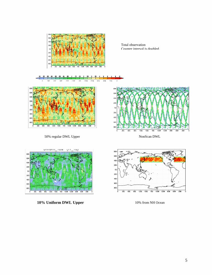
Total observation

Counter interval is doubled.

NonScan DWL

10% Uniform DWL Upper

50% regular DWL Upper

10% Uniform DWL Upper 10% from NH Ocean

5

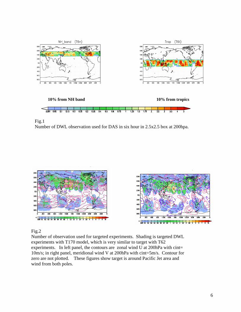
10% from NH band 10% from tropics

Fig.1 Number of DWL observation used for DAS in six hour in 2.5x2.5 box at 200hpa.

Fig.2 Number of observation used for targeted experiments. Shading is targeted DWL experiments with T170 model, which is very similar to target with T62 experiments. In left panel, the contours are zonal wind U at 200hPa with cint= 10m/s; in right panel, meridional wind V at 200hPa with cint=5m/s. Contour for zero are not plotted. These figures show target is around Pacific Jet area and wind from both poles.

6

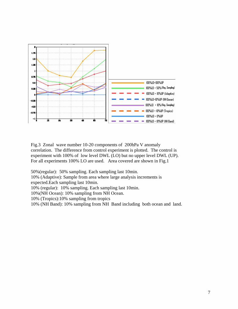
Fig.3 Zonal wave number 10-20 components of 200hPa V anomaly correlation. The difference from control experiment is plotted. The control is experiment with 100% of low level DWL (LO) but no upper level DWL (UP). For all experiments 100% LO are used. Area covered are shown in Fig.1 50%(regular): 50% sampling. Each sampling last 10min. 10% (Adaptive): Sample from area where large analysis increments is expected.Each sampling last 10min. 10% (regular): 10% sampling. Each sampling last 10min. 10%(NH Ocean): 10% sampling from NH Ocean. 10% (Tropics):10% sampling from tropics 10% (NH Band): 10% sampling from NH Band including both ocean and land.

7

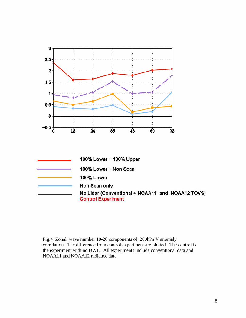
Fig.4 Zonal wave number 10-20 components of 200hPa V anomaly correlation. The difference from control experiment are plotted. The control is the experiment with no DWL. All experiments include conventional data and NOAA11 and NOAA12 radiance data.

8

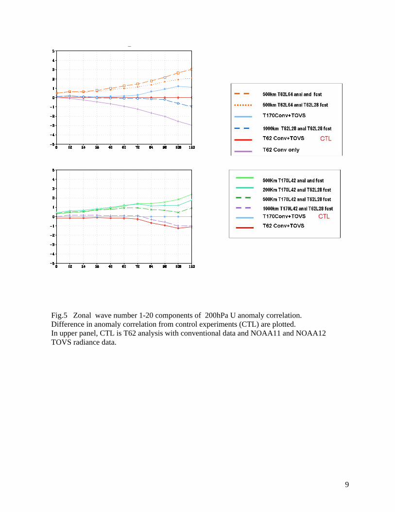
Fig.5 Zonal wave number 1-20 components of 200hPa U anomaly correlation. Difference in anomaly correlation from control experiments (CTL) are plotted. In upper panel, CTL is T62 analysis with conventional data and NOAA11 and NOAA12 TOVS radiance data.

9

U200hPa T200hPa

T 200 hPa

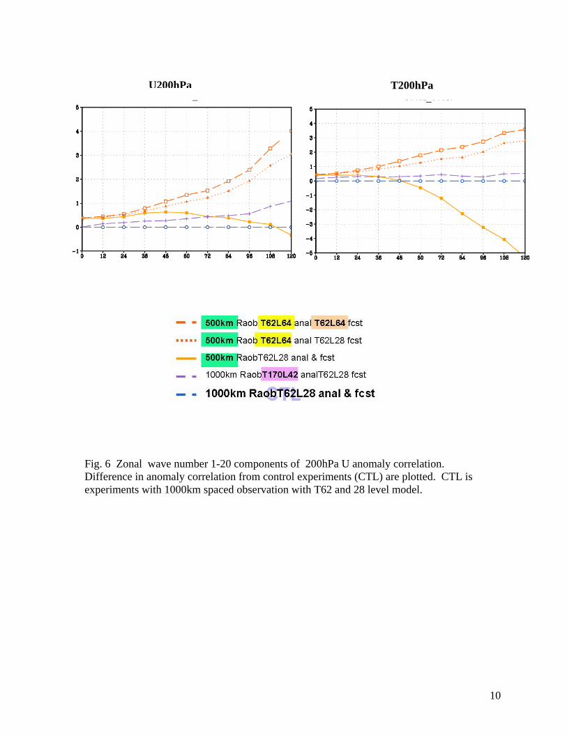
Fig.5 Fig. 6 Zonal wave number 1-20 components of 200hPa U anomaly correlation. Difference in anomaly correlation from control experiments (CTL) are plotted. CTL is experiments with 1000km spaced observation with T62 and 28 level model.

10

U200hPa T200hPa

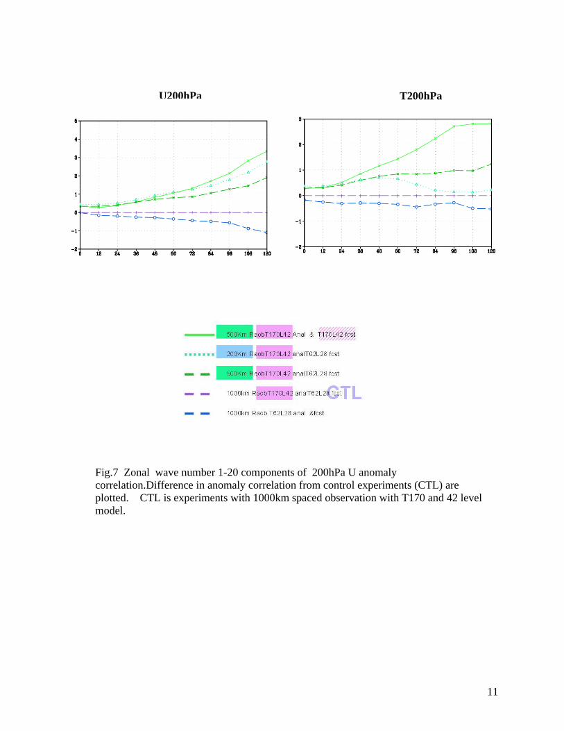
Fig.7 Zonal wave number 1-20 components of 200hPa U anomaly correlation.Difference in anomaly correlation from control experiments (CTL) are plotted. CTL is experiments with 1000km spaced observation with T170 and 42 level model.

11