simulation of titration experiments -...
TRANSCRIPT

CHEMISTRY
Simulation of titration experiments
Academic Year 2010-2011
UNIVERSITE DE MAROUA …………………
ECOLE NORMALE SUPERIEURE ………………
DEPARTEMENT DE CHIMIE
THE UNIVERSITY OF MAROUA ………………
HIGHER TEACHERS’ TRAINING COLLEGE ……………….
DEPARTMENT OF CHEMISTRY
A dissertation submitted in partial fulfillment of the requirements for the award of the postgraduate teachers’ Diploma (DIPES II)
By
KENGNE Enselme (BSc. Chemistry; University of Yaoundé I)
Supervisor
ABDOUL WAHABOU
Senior lecturer
Simulation of titration experiments
i
Dedication
To my mother
Who sacrificed her youth to educate us but could not reap the fruits of her
labour.

Simulation of titration experiments
ii
Acknowledgments
We wish to express our deep gratefulness and appreciation to our principal
supervisors Dr ABDOUL Wahabou for his great, support, thoughts, encouragements,
and guidance. We also wish to express our profound gratitude and appreciation to our
others supervisor, Mr. Abdoul N. Rahman for his invaluable suggestions, support,
ideas, comments and continuous guidance throughout study. This work would not
have been completed without their thoughtful encouragements.
We glorify Jesus, the lord of lords, for his huge love, his matchless and peerless
faithful.
We wish to thank our parents, family members and friends who gave us moral,
financial and material support through out our stay in Maroua. Amongst others, we
have: Mrs. WABO Colette, Dr. FOTSO Emmanuel, Mrs. TATIEFO Jacqueline, and
M. KUATE Gilbert, Mrs. YIMGA Virginie, Mrs. TALA Hortense, M. SIKADI
Francis Bebey, M. TAGNE Simplice and all theirs husbands and wives. May this piece
of work portray a real testimony of my profound gratitude for their tireless love and
care. May the good GOD continue to bless them in all their endeavours.
Finally, we are thankful to our nephews and nieces who provided us with joy
and happiness, their love made this work possible. We will be indebted throughout our
life to our parents, Marie Pascale MEGNE and father David TAGNE who sacrificed
their life for our education.
We won’t forget our mentor M. NGANTCHOU Serge, M. YIMGA André
Marie and M. MTOPI Joseph Frederix for their guidance through out our stay in
Maroua. We shall always remember Mrs.
Special thanks to our teachers of the department of chemistry to the higher teacher’s
training college to the University of Maroua, our classmates and all those whose
names are not mentioned above. We plead that this work portrays a profound
expression of our acknowledgements.

Simulation of titration experiments
iii
Table of contents Dedication ............................................................................................................... i
Acknowledgments .................................................................................................. ii
Abstract .................................................................................................................. v
Résume .................................................................................................................. vi
List of tables ......................................................................................................... vii
List of figures....................................................................................................... viii
General introduction ............................................................................................... 1
CHAPTER I: GENERALITIES ON CHEMICAL ANALYSIS ........................ 3
Introduction ............................................................................................................ 3
I.1 Chemical analysis ........................................................................................... 3
I.1.1 Qualitative analysis .................................................................................. 4
I.1.2 Quantitative analysis ................................................................................ 4
I.1.3 Methods of chemical analysis ................................................................... 5
I.2 Data calculations ............................................................................................ 6
I.2.1 Measurement of physical quantities .......................................................... 6
I.2.2 Units of measurement ............................................................................... 6
I.3 Notion of acids and bases ............................................................................... 9
I.3.2 Acidity and alkalinity ............................................................................. 11
I.4 Notion of oxidation-reduction ....................................................................... 13
I.4.1 Definition ............................................................................................... 13
I.4.2 Oxidation-reduction reactions................................................................. 14
I.5 Coloured indicators………………………………………………………......14
I.6 Notion of concentration ................................................................................ 16
I.6.1 Molarity ................................................................................................. 16
I.6.2 Normality ............................................................................................... 17
I.6.3 Ponderal concentration ........................................................................... 17
I.6.4 Percentage by mass ................................................................................ 17
I.6.5 Molality.................................................................................................. 18
Simulation of titration experiments
iv
CHAPTER II: TITRATION .............................................................................. 19
II.1 Introduction ................................................................................................. 19
II.2 Acid-base titrations ..................................................................................... 20
II.2.1 Experiment nº1 ..................................................................................... 22
II.3 Oxidation-reduction titrations ...................................................................... 26
II.3.1 Experiment nº2: .................................................................................... 26
CHAPTER III: NUMERICAL METHODS AND SIMULATION .................. 31
III.1 Numerical methods .................................................................................... 31
III.1.1 General principle of numerical methods ............................................... 31
III.1.2 Principal numerical methods ................................................................ 31
III.2 Simulation ................................................................................................. 34
III.2.1 Definitions ........................................................................................... 34
III.2.2 Simulation of an acid-base titration ...................................................... 35
III.2.3 Simulation of an oxidation-reduction titration ...................................... 40
III.3 Discussion of results .................................................................................. 44
III.4 Conclusion and recommendations .............................................................. 47
References ............................................................................................................ 48
Appendices ........................................................................................................... 50
Simulation of titration experiments
v
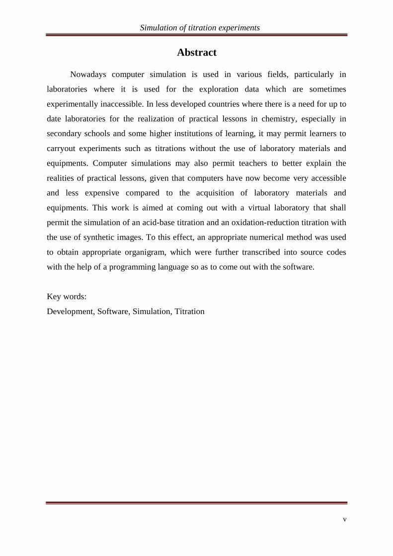
Abstract
Nowadays computer simulation is used in various fields, particularly in
laboratories where it is used for the exploration data which are sometimes
experimentally inaccessible. In less developed countries where there is a need for up to
date laboratories for the realization of practical lessons in chemistry, especially in
secondary schools and some higher institutions of learning, it may permit learners to
carryout experiments such as titrations without the use of laboratory materials and
equipments. Computer simulations may also permit teachers to better explain the
realities of practical lessons, given that computers have now become very accessible
and less expensive compared to the acquisition of laboratory materials and
equipments. This work is aimed at coming out with a virtual laboratory that shall
permit the simulation of an acid-base titration and an oxidation-reduction titration with
the use of synthetic images. To this effect, an appropriate numerical method was used
to obtain appropriate organigram, which were further transcribed into source codes
with the help of a programming language so as to come out with the software.
Key words:
Development, Software, Simulation, Titration
Simulation of titration experiments
vi
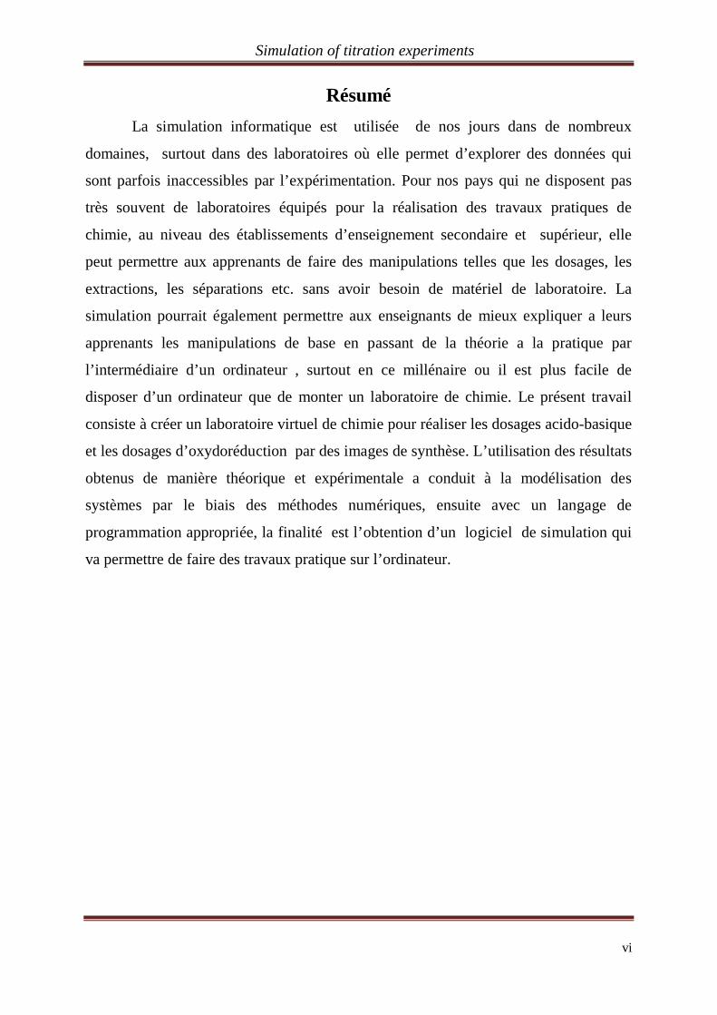
Résumé
La simulation informatique est utilisée de nos jours dans de nombreux
domaines, surtout dans des laboratoires où elle permet d’explorer des données qui
sont parfois inaccessibles par l’expérimentation. Pour nos pays qui ne disposent pas
très souvent de laboratoires équipés pour la réalisation des travaux pratiques de
chimie, au niveau des établissements d’enseignement secondaire et supérieur, elle
peut permettre aux apprenants de faire des manipulations telles que les dosages, les
extractions, les séparations etc. sans avoir besoin de matériel de laboratoire. La
simulation pourrait également permettre aux enseignants de mieux expliquer a leurs
apprenants les manipulations de base en passant de la théorie a la pratique par
l’intermédiaire d’un ordinateur , surtout en ce millénaire ou il est plus facile de
disposer d’un ordinateur que de monter un laboratoire de chimie. Le présent travail
consiste à créer un laboratoire virtuel de chimie pour réaliser les dosages acido-basique
et les dosages d’oxydoréduction par des images de synthèse. L’utilisation des résultats
obtenus de manière théorique et expérimentale a conduit à la modélisation des
systèmes par le biais des méthodes numériques, ensuite avec un langage de
programmation appropriée, la finalité est l’obtention d’un logiciel de simulation qui
va permettre de faire des travaux pratique sur l’ordinateur.
Simulation of titration experiments
vii
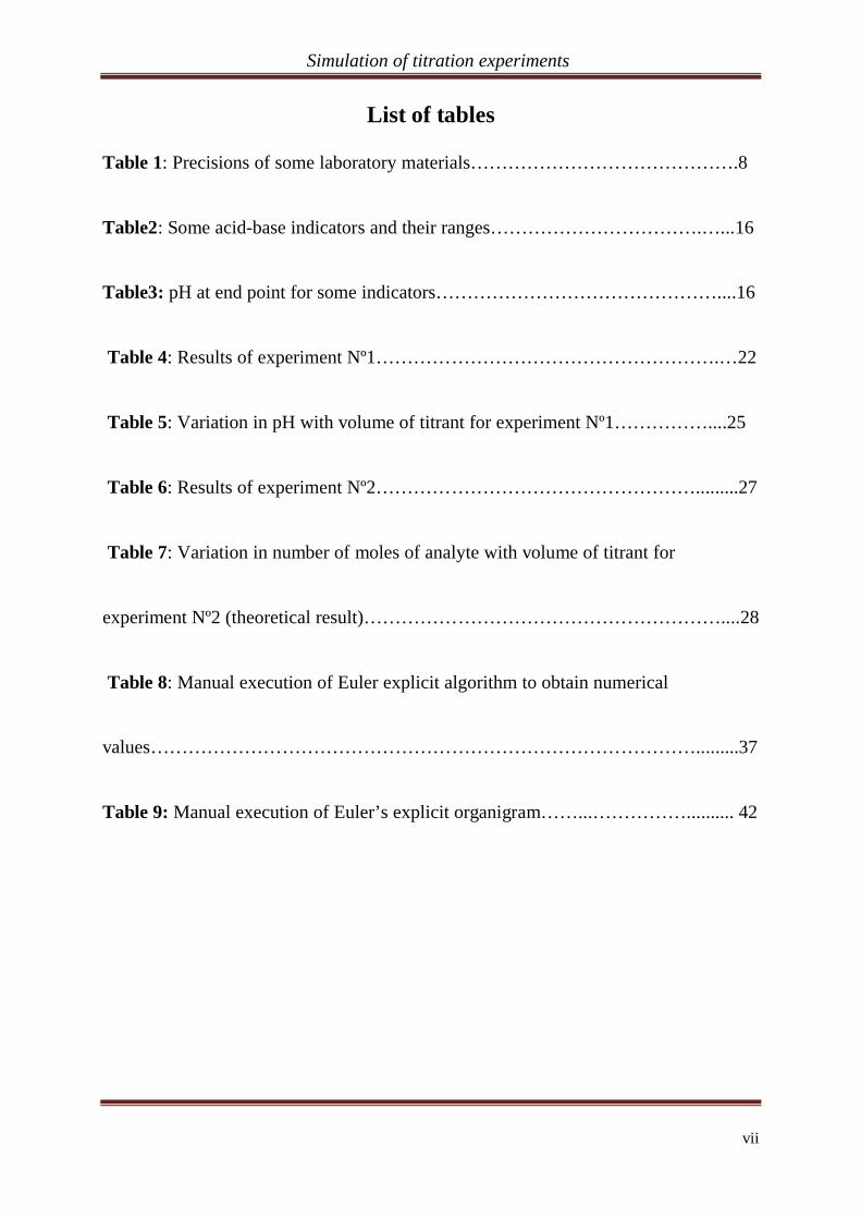
List of tables
Table 1: Precisions of some laboratory materials…………………………………….8
Table2: Some acid-base indicators and their ranges…………………………….…...16
Table3: pH at end point for some indicators………………………………………....16
Table 4: Results of experiment Nº1……………………………………………….…22
Table 5: Variation in pH with volume of titrant for experiment Nº1……………....25
Table 6: Results of experiment Nº2…………………………………………….........27
Table 7: Variation in number of moles of analyte with volume of titrant for
experiment Nº2 (theoretical result)…………………………………………………....28
Table 8: Manual execution of Euler explicit algorithm to obtain numerical
values…………………………………………………………………………….........37
Table 9: Manual execution of Euler’s explicit organigram……...…………….......... 42
Simulation of titration experiments
viii
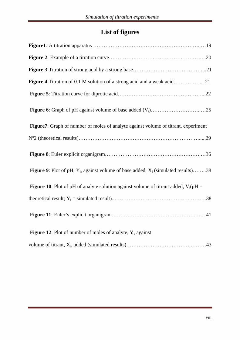
List of figures
Figure1: A titration apparatus ……………………………………………………..…19
Figure 2: Example of a titration curve………………………………………………..20
Figure 3:Titration of strong acid by a strong base…………………………………....21
Figure 4:Titration of 0.1 M solution of a strong acid and a weak acid……………... 21
Figure 5: Titration curve for diprotic acid…………………………………………...22
Figure 6: Graph of pH against volume of base added (Vi)………………………..…25
Figure7: Graph of number of moles of analyte against volume of titrant, experiment
Nº2 (theoretical results)…………………………………………………………….....29
Figure 8: Euler explicit organigram……………………………………………….…36
Figure 9: Plot of pH, Yi, against volume of base added, Xi (simulated results)……..38
Figure 10: Plot of pH of analyte solution against volume of titrant added, Vi(pH =
theoretical result; Yi = simulated result)..…………………………………….……….38
Figure 11: Euler’s explicit organigram………………………………………….….. 41
Figure 12: Plot of number of moles of analyte, Y , against
volume of titrant, X , added (simulated results)……………………………….………43
Simulation of titration experiments
1
General introduction
Active pedagogy is one of the various methods of experimental learning that is
“learning by doing”. Here, the learner is put in a situation where he or she uses his or
her initiatives so as to improve on his or her competences [1]. This method of learning
is only applicable to all experimental sciences such as Chemistry, Biology and Physics
etc, where the primordial or principal objectives can only be attained if and only if
theory is incorporated with practical. The teaching of Chemistry, particularly solution
Chemistry in secondary schools as well as some higher institutions of learning in
Cameroon is more or less becoming theoretical if not mathematical. The assimilation
of most notions and concepts becomes more and more difficult due to the lack of
adequate didactic materials [2]. The realization of practical lessons, which is of
utmost importance as far as this subject is concerned, becomes very difficult due to the
following reasons:
-The complete absence of laboratories in most secondary schools and some higher
institutions of learning,
-The lack of up to date laboratories in a case where they exist,
-The very high cost of laboratory materials and chemicals,
-The difficult storage conditions and the dangers involved in certain experimental
manipulations etc.
With the evolution of computer science ever since the 1990s, virtual reality has
become very indispensable for the exploration and manipulation of experimental data,
a situation which was at first impossible [3]. General Chemistry and particularly
solution Chemistry has therefore become one of the domains that make use of
computer simulation. Thus the use of computer simulation in the teaching of titrations
for instance, may serve as an alternate pedagogic method to this effect. This method
can henceforth be used for the verification, investigation, forecasting and the analysis
of acid-base phenomena. Here, the learner is expected to pay much attention to the
analysis of purely chemical phenomena while neglecting all superficial numerical
calculations. In this way the learner is able to give a detailed interpretation of the
observations made in an experiment. With the possibility of modifying the system,
Simulation of titration experiments
2
constants and variables, simulation would enable the teacher to better prepare and
execute his practical lessons [1, 4]. With the aim of contributing our own quota to the
enormous research that has been carried out so far in the didactics of chemistry, we
will carry out the simulation of titrations with the aid of a device-software, conceived
for the realization of practical lessons in chemistry. To this effect, we shall commence
with a presentation of the basic concepts in analytical chemistry. Thereafter, we shall
carry out a brief review of some of the numerous numerical methods used in the
modeling of natural and artificial systems before proceeding with the simulations.
Finally, we will come out with the merits and the demerits of this method.

Simulation of titration experiments
3
CHAPTER I: GENERALITIES ON CHEMICAL ANALYSIS
Introduction
One of the primordial preoccupations during the days of Antoine Lavoisier in
chemistry was the determination of elements, in other words the constituents of
various compounds. Various methods were therefore required to split or break down
complex substances or compounds and to characterize the different elementary
products obtained [5]. What ever the type of experiment that has to be carried out on a
sample in a chemical laboratory, certain factors have to be taken into consideration so
as to obtain better results. This takes place by the determination of the type of analysis
to be carried out, its nature and the protocols to be respected in order to obtain the
different parameters and quantities that describe the physical and chemical identities of
the substance under study in the sample.
I.1 Chemical analysis
Analytical chemistry is a branch in chemistry that deals with the analysis-that is
the separation, identification and quantification of the chemical components of natural
and artificial materials [6]. Mean while chemical analysis is a technique used in the
identification and quantification of a sample [7]. Rapid chemical analysis is the
separation of pure substances from a mixture; while elementary analysis deals with the
separation of the constituents of a compound. There exist various types of analysis, all
of which may be classified under qualitative analysis, quantitative analysis, chemical
methods and physicochemical methods. Qualitative analysis deals with the
identification of the constituents of a compound or mixture, while quantitative analysis
deals with the determination of the amounts of the various constituents present in the
sample [8].
Simulation of titration experiments
4
I.1.1 Qualitative analysis
This technique permits to identify the various substances present in a sample.
Here majority of the operations occur in aqueous solution-that is in water and helps to
isolate ions easily. Ions in solution can be isolated or separated by the following
methods:
- Precipitation;
- Oxidation-reduction reaction;
- Formation of a complex, or
- The formation of covalent or ionic compounds, amongst which precipitation is the
most effective and efficient. Once formed, the precipitate is separated from the
solution by decantation. Other methods such as distillation, solvent extraction or ion
exchange can also be used to separate a given ion from a solution [9].
I.1.2 Quantitative analysis
Quantitative analysis deals with the determination of the amounts of the
different constituents of a substance. There are two main types of quantitative analysis
namely gravimetric analysis and volumetric analysis, where volumetric analysis is the
most rapid and less precise. Gravimetric analysis involves determining the amounts of
the constituents of a compound or mixture by weighing with the use of a balance.
Generally, this takes place by selective precipitation of the constituents, followed by
drying to obtain a constant mass. The mass may then be expressed in terms of
percentage. In volumetric analysis, a given volume of a solution with a known
concentration is reacted with a know volume of a second solution whose concentration
is not known. The unknown concentration can then be calculated (in gram per litre,
mol per litre, equivalent gram per litre, percentage by mass or in parts per million)
knowing the number of equivalence of the substances concerned. Generally, at the
equivalence point of a reaction:
A + B C or A B, the number of equivalent gram of A equals
the number of equivalent gram of B: =

Simulation of titration experiments
5
And the relative errors: = + +
The volumes and are measured precisely with the use of equipments such as
pipettes, burettes, measuring cylinders and volumetric flasks etc. (see standardization
of burettes, pipettes etc).
In quantitative analysis, and particularly volumetric analysis, the reaction taking place:
- should be fast and complete
- should be stoichiometric and occur in a single step, and
- have an easily identifiable equivalence point.
Back titration method is usually used in a case where there is no equilibrium even
though the reaction is complete and stoichiometric. Chemical methods (coloured
indicators), electrochemical methods (pH, conductivity etc) or physical methods are
then used to titrate the excess titrant. The indicator changes colour at the equivalence
point. At this point, the number of moles of the titrant equals that of the analyte or
titrant.
The different types of reactions used in volumetric analysis include:
- Acid-base reactions,
- Oxidation-reduction reactions,
- Precipitation reactions and,
- Complex formation.
Titrations are possible if the concentration of one of the solutions is known: this is the
standard solution, and it is obtained by weighing a precise mass of a substance called a
primary standard [7,9].
I.1.3 Methods of chemical analysis
There exist two types of analytical methods namely: chemical methods and
physicochemical methods involving chemical or electrochemical reactions and purely
physical methods that make use of the physical properties of matter.
Chemical methods include gravimetric method and volumetric method. The former,
deals with the weighing of a compound obtained by selective precipitation. An
example is the determination of the concentration of chloride ions in a solution of
Simulation of titration experiments
6
silver chloride. The latter makes use of volume measurements during titrations to
determine the concentration of a substance.
I.2 Data collection and calculation
I.2.1 Measurement of physical quantities
The objective in every experiment is to obtain one or more numerical results.
This usually entails the calculation of quantities such as mean etc, in order to allow for
uniformity of values obtained. To this effect, we have to evaluate the variance which
does not only give an idea on the statistical error committed, but also the systematic
error. The value of a physical quantity obtained is meaningful if and only if its
uncertainty is also given. In other words, the validity of an experimental result with
respect to the theoretical value depends on the uncertainty. The evaluation of the
uncertainty supposes that we have an idea on the precision of the measuring
instruments. It also shows the influence errors have on a result [7].
I.2.2 Units of measurement
The measurement of a physical quantity makes use of two factors: the value and
the unit of measurement or simply unit. This explains why units are always precised in
all exercises involving physical quantities. Like other quantities, units of
measurements may be obtained through mathematical operations such as
multiplication, division, addition or subtraction. For instance the surface area, A, of a
piece of silver wire of length L and width W is obtained by multiplying the values and
the units as well. That is: A = L x W = 3.00cm x 5.00cm =15.00cm2. At times when
dividing, the units may cancel out each other. In case of any doubt in the operation to
undertake, check the available units [7, 9, and 11].
I.2.3 Manipulation of experimental results
All scientific laws are based on the regularity or coherence in experimental
observations. The observer therefore has to take into consideration the limit of validity,
Simulation of titration experiments
7
of the data from which deductions are made. A great deal of measures has to be taken
during the collection of data. Statistically, a sufficient number of values have to be
obtained in order to come out with a value approximately equal to the exact one.
Analytical techniques equally determine the number of measurements to be carried
out. This explains why it is very important to evaluate the mean value and the
precision which gives the uncertainty on the measured values.
I.2.3.1 Statistical and systematic errors
Slightly different results obtained discretely with the same instrument are said
to possess statistical errors. This error is annulled or corrected by evaluating the mean
of a handful of independent values. Very often, the value obtained after the elimination
of the statistical error still possess some uncertainty due to the characteristics of the
instrument and the technique used in measurement. This error is known as systematic
error. An example of such an error is that due to poor graduation of an instrument, loss
of material (e.g. a gas in a system under pressure or in a vacuum), non respect of
measuring conditions (e.g. incomplete reaction in a calorimeter, incomplete
dehydration of a precipitate etc) or other recurrent operational errors (e.g. poor reflex,
personal preference etc). These systematic errors are said to be « determined » because
they can be corrected or eliminated or evaluated by the application of practical
measurement: the use of graduation, reference substances or other experimental
conditions. If we consider an error to be the difference between the value observed and
the measured value, it can obviously be minimised if there is coherence between a
handful of independent values [7, 11].
I.2.3.2 Precision and exactitude
The uncertainty of a value is reflected in the precision and the exactitude. This
uncertainty provides a clue in the validity of the results obtained. It is therefore of
utmost importance to have a very precise and exact data. Exactitude supposes that a
great number of values are more or less close to a certain value so as to allow for a
better precision. The precision of a numerical result expresses the reproductivity of a
Simulation of titration experiments
8
result obtained several times with the same instrument, and thus gives the uncertainty
due to statistical error. Exactitude is a measure of the accord between the « best »
value and the « true » value or the accepted value. It is therefore difficult to give the
exactitude of a given value because of systematic and statistical errors. Exact values
are found in handbooks, and have been obtained by evaluating the mean of different
values obtained through different procedures, by competent researchers using well
graduated equipments of highly accepted standards under well defined experimental
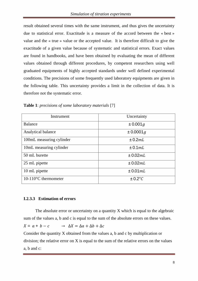
conditions. The precisions of some frequently used laboratory equipments are given in
the following table. This uncertainty provides a limit in the collection of data. It is
therefore not the systematic error.
Table 1: precisions of some laboratory materials [7]
Instrument Uncertainty
Balance ±0.001
Analytical balance ±0.0001
100mL measuring cylinder ±0.2
10mL measuring cylinder ±0.1
50 mL burette ±0.02
25 mL pipette ±0.02
10 mL pipette ±0.01
10-110°C thermometer ±0.2°
I.2.3.3 Estimation of errors
The absolute error or uncertainty on a quantity X which is equal to the algebraic
sum of the values a, b and c is equal to the sum of the absolute errors on these values.
= +
Consider the quantity X obtained from the values a, b and c by multiplication or
division; the relative error on X is equal to the sum of the relative errors on the values
a, b and c:
Simulation of titration experiments
9
=+
= + +
I.3 Notion of acids and bases
The terms acid and base may be defined in various ways according to different
authors.
Arrhenius’ theory
An acid is a substance that dissociates in water to liberate hydrogen ions or protons
(H+) [12]. The dissociation equation of hydrochloric acid, ( ), in water can be
represented as follows:
( ) ( ) + ( )
The concentration of the acid in the resulting solution is far greater than that of
hydrogen ions in pure water. Similarly, a base is a substance that dissociates in water
to liberate hydroxide ions (OH-). +
The definition of an acid and a base by Arrhenius is insufficient, firstly in the sense
that he did not consider the case of substances that do not dissolve in water (e.g.
hydrogen chloride), secondly because some acids do not possess hydrogen atoms (e.g.
BF3) and that not all bases would liberate hydroxide ions in water (e.g. NH3).
The Lowry-Bronsted theory
According to Lowry-Bronsted, an acid is a proton donor, while a base is a
proton acceptor. Therefore all acids, according to this theory contain one or more
hydrogen atoms and that not all compounds containing hydrogen atoms are acids (e.g.
NaH and CH4). Also an acid that contains one replaceable hydrogen ion is called a
monoacid (e.g. HCl), while an acid that contains two or more replaceable hydrogen
ions is respectively said to be dibasic (e.g. H2SO4) or a polyacid. On the other hand, a
Simulation of titration experiments
10
monobase is one that can only accept one mole of hydrogen ions, while a dibase or
polybase is one that can accept two or more moles or hydrogen ions respectively.
Generally, a Bronsted-Lowry acid is denoted HA, while the base is denoted B. The
Bronsted-Lowry definition of an acid and a base can therefore be represented by the
following reaction equations: [12-13].
+
+ +
From the above two equations, it follows that an acid can only lose a proton in the
presence of a base. This brings us to the notion of acid-base couple [12].
( ) ( )
+
The Lewis theory
According to Lewis, an acid is an electron pair acceptor, while a base is an
electron pair donor. In this theory, when an acid reacts with a base, they form a
complex resulting from the sharing of a pair of electrons donated by the base in a
dative bonding. For instance, if A is a Lewis acid and B a Lewis base, we can
write:
A: + B A B, that is: acid + base complex
This theory is advantageous in the sense that it is also applicable to solvents other than
water and does not involve acid-base conjugates, talk less of the strength. In this way,
ammonia behaves like a base by donating a pair of electrons to boron trifluoride to
form a complex compound as depicted by the following reaction equation:
H3N: + BF3 H3N BF3
Note that the definition of an acid and a base by Lewis is very general because it
equally takes into consideration the Bronsted-Lowry acids and bases. [12-13-14].
Simulation of titration experiments
11
I.3.2 Acidity and alkalinity
The acidity and the alkalinity of a medium can be measured with the use of a
pH scale. A pH scale is a scale on a pH-meter with values ranging from 0 to 14. The
pH of a neutral solution such as pure water at 25 °C is equal to 7, for an acidic
solution, the pH is less than 7, while the pH of a basic solution is greater than 7. For
acids, the strength increases with decreasing pH, while the strength of bases increases
with increasing pH.
In aqueous solution, pH is the negative logarithm to the base 10 of the molar hydrogen
ion concentration. That is : = [ ( )]
Acid-base reactions
An acid-base reaction involves two acid-base couples: that is acid1/base1 and
acid2/base2 [12]. It is a reaction that involves the exchange or transfer of hydrogen ions
from the acid of one couple to the base of a second couple.
The overall equation of the reaction can easily be obtained by first of all writing the
half equations with respect to each specie, after which the two half equations are added
in a way such that all the hydrogen ions are eliminated. That is:
- acid1 base1 + nH +
- base2 + nH + acid2
- acid1 + base2 base1 + acid2 (overall equation)
Example
When a solution of sodium hydroxide ( ( ), ( )) is added to a solution of
ammonium chloride ( ( ), ( )), ammonia gas ( ) is liberated. In this
reaction, the participation of sodium ions ( ( )) and chloride ions ( ( )) are more
or less invissible. They are said to be spectator ions, thereby leading to the transfer of
hydrogen ions from the acid ( ( )) to the base ( ) we therefore write:
+
+
Simulation of titration experiments
12
That is: ( ) + ( )) ( ) + ( ).
The equilibrium position depends on the values of the different couples
concerned. In this example, ( / > ( / and as such the
reaction is more to the right (i.e. is a weak base) [12].
Dissociation constants of acids and bases
An acid-base reaction is a reaction involving the transfer of one or more hydrogen
ions in aqueous solution. The specie that accepts the hydrogen ions is called a base,
while the one that loses is called an acid.
Although the pH of a solution provides some measure of the strength of the constituent
acid or base, the use of pH is very limited in this context due to the fact that its value
changes as the concentration changes.
It is in this light that chemists had to come out with a more useful, yet quantitative,
means of representing the strength of acids and bases-by considering the dissociation
equilibria of these substances in aqueous solution7.
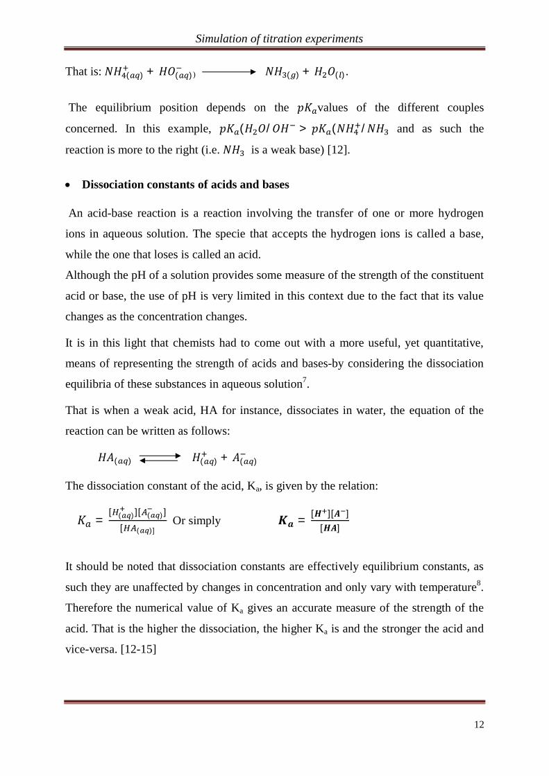
That is when a weak acid, HA for instance, dissociates in water, the equation of the
reaction can be written as follows:
( ) ( ) + ( )
The dissociation constant of the acid, Ka, is given by the relation:
=[ ( )][ ( )]
[ ( )] Or simply = [ ][ ]
[ ]
It should be noted that dissociation constants are effectively equilibrium constants, as
such they are unaffected by changes in concentration and only vary with temperature8.
Therefore the numerical value of Ka gives an accurate measure of the strength of the
acid. That is the higher the dissociation, the higher Ka is and the stronger the acid and
vice-versa. [12-15]
Simulation of titration experiments
13
By analogy with the dissociation constant of a weak acid, the dissociation
constant, Kb, for a weak base, BOH, can be obtained from its dissociation equation as
follows:
( ) ( ) + ( )
= [ ][ ][ ]
Here also, the strength of the base increases with increasing Kb.
I.4 Notion of oxidation-reduction
Oxidation and reduction go hand in hand or are complementary processes.
Therefore, every oxidation must be accompanied by a reduction and vice-versa. At
first, chemists had a very limited view of redox, using it to account for only the
reactions of oxygen and hydrogen. Now our days, ideas of redox have been extended
to include all electron-transfer process [12].
I.4.1 Definition
The terms oxidation and reduction can be defined in various ways. The most
appropriate of all being that in terms of electrons, even though not all processes
involve a complete transfer of electrons.
Oxidation: It is the removal of electrons from a substance.
The following two equations depict the loss of electrons by an atom of sodium ( )
and an iron (II) ion ( ) to form a sodium ion, , and an iron(III) ion,
respectively.
+
+
Here, both the sodium atom and the iron (II) ion have been oxidized.
Reduction: It is the gain of electrons by a substance.

Simulation of titration experiments
14
For example;
( ) + 2 2
+ 2
It should be noted that, the definition of oxidation and reduction in terms of electrons
is very general, even though not all processes involve a complete loss or gain (transfer)
of electrons.
I.4.2 Oxidation-reduction reactions
An oxidation-reduction reaction is a reaction in which oxidation and reduction occur
simultaneously.
It is usually of the form:
+ +
In the above equation, is the oxidizing agent or oxidant which is reduced to
, while is the reducing agent which is oxidized to . An example of a
redox reaction is the oxidation of iron (II) ions by permanganate ions in acidic
medium.
( ) + 5 ( ) + 8 ( ) ( ) + 5 ( ) + 4 ( )
In a redox reaction, the substance that gains electrons is called the oxidizing
agent and the one that loses electrons is called the reducing agent. In the course of the
reaction, the reducing agent is oxidized, while the oxidizing agent is reduced.
I.5 Coloured indicators
Definition
A coloured indicator is a macro molecular weak organic acid or base having
different colours in the molecular and ionic forms [12]. For instance, the ionisation
equation of methyl orange can be represented by the following:
+
Red yellow

Simulation of titration experiments
15
They are usually used to test the alkalinity and acidity of a solution and to detect the
end point of acid-base reactions. They change colour according to the hydrogen ion
concentration of the solution or liquid to which they are added. Some examples of
acid-base indicators are: methyl orange, phenolphthalein, litmus, bromothymol blue,
methyl red etc. [18].
Action of acid-base indicators
An indicator may be considered as a weak acid-weak base conjugate pair (according to
Bronsted-Lowry). If we denote InH the acid form and In- the basic form of an
indicator, then the equilibrium between the two forms is given by the following
equation:
The dissociation constant of the acid, is given by
Where [ ] is the concentration of the species in mol.l-1
Very often, we use which is the negative logarithm to the base 10 of :
.Each indicator is characterized by a value or of many pKi values
in the case of a polyacid. Also, an addition of a base to the equilibrium mixture causes
the equilibrium position to shift to the right according to le Chartelier’s principle; as
such the colour of the ionic form prevails. Meanwhile, if an acid is added to the
equilibrium mixture, the equilibrium position shifts to the left and the colour of the
molecular form prevails.
The range of an indicator
Around the end point of an acid-base reaction, both coloured forms of the indicator
will be present in appreciable quantities. The range of an indicator is the pH range over
which it changes colour [18].
Simulation of titration experiments
16
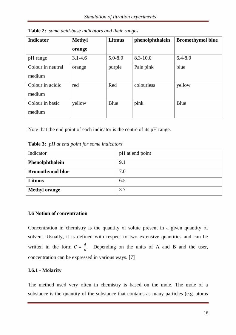
Table 2: some acid-base indicators and their ranges
Indicator Methyl
orange
Litmus phenolphthalein Bromothymol blue
pH range 3.1-4.6 5.0-8.0 8.3-10.0 6.4-8.0
Colour in neutral
medium
orange purple Pale pink blue
Colour in acidic
medium
red Red colourless yellow
Colour in basic
medium
yellow Blue pink Blue
Note that the end point of each indicator is the centre of its pH range.
Table 3: pH at end point for some indicators
Indicator pH at end point
Phenolphthalein 9.1
Bromothymol blue 7.0
Litmus 6.5
Methyl orange 3.7
I.6 Notion of concentration
Concentration in chemistry is the quantity of solute present in a given quantity of
solvent. Usually, it is defined with respect to two extensive quantities and can be
written in the form = . Depending on the units of A and B and the user,
concentration can be expressed in various ways. [7]
I.6.1 - Molarity
The method used very often in chemistry is based on the mole. The mole of a
substance is the quantity of the substance that contains as many particles (e.g. atoms

Simulation of titration experiments
17
electrons ions molecules etc) as there are in 12g of an atom of carbon-12. This quantity
denoted , = 6.02 10 is called the Avogadro number.
The molarity, , of a solution is defined as = ( / ) , where n is the number of
moles of solute and V is the volume of the solution in litres. [7, 11]
I.6.2 Normality
Concentration can also be expressed in terms of equivalent gram. The
equivalent gram of a substance is the quantity of substance that would liberate or
consume one mole of hydrogen ions or proton (in the case of an acid-base reaction) or
one mole of electrons (in the case of an oxidation-reduction reaction). This quantity
denoted N, is called normality and is defined by = (eqg/L) (where ne is the
number of equivalent gram of solute and V is the volume of the solution in litres. This
method is usually used in calculations during reactions without taking into
consideration the stoichiometric coefficients in the balanced equation.
Dividing N by C, we obtain:
= = = , where x is the number of equivalent gram per mole of
substance [7, 11]
I.6.3 Ponderal concentration
Ponderal concentration, P, is the mass in grams of solute per litre of solution. That is
= (g/L), where m is the mass of solute and V the volume of solution (in litres.)
Knowing that = , we deduce that = or = .
I.6.4 Percentage by mass
Concentration may also be expressed in terms of percentage by mass. That is ;
% = × 100, where m is the mass of the solute and is the mass of the
solution. But the mass of the solution is given by = m + 1000V, where
= 1000 / is the density of the solvent (water).
Simulation of titration experiments
18
Thus % = × 100 = × 100
This method of calculation of concentration is mostly used by pharmacists and medical
doctors during the titration of medicines [7, 11]
I.6.5 Molality
The above mentioned expressions for concentration are disadvantageous in the sense
that, they all depend on the volume of the solution and would thus vary with changes
in temperature. This difficulty can be overcomed with the use of molality. The
molality of a solution denoted , is the number of moles of solute per kilogram of
solvent. That is; = (mol/Kg). This implies = , where M is the molar
mass, the density, n is the number of moles of solute and is the mass of solvent in
kilograms [7, 11]
Simulation of titration experiments
19
CHAPTER II: TITRATION
II.1 Introduction
Titration is a common laboratory method or technique used in volumetric analysis
to determine the concentration of a solution, where a solution called the titrant or
titrator of a known concentration from a graduated burette or pipetting syringe is
added to a known volume of a second solution called the analyte or titrand of unknown
concentration until the chemical reaction between the two solutions is just complete
(equivalence point) [16]. The equivalence point or end point of the titration
corresponds to the volume of the added titrant at which the number of moles of the
titrant is equal to the number of moles of the analyte or some multiple thereof (e.g. in
the case of polyprotic acids). It is usually indicated by a permanent change in colour,
and at this point all of the analyte have been consumed or transformed [16].Usually,
the equivalence point is indicated with the aid of a pH indicator or a potentiometer or a
pH metre or colour change.
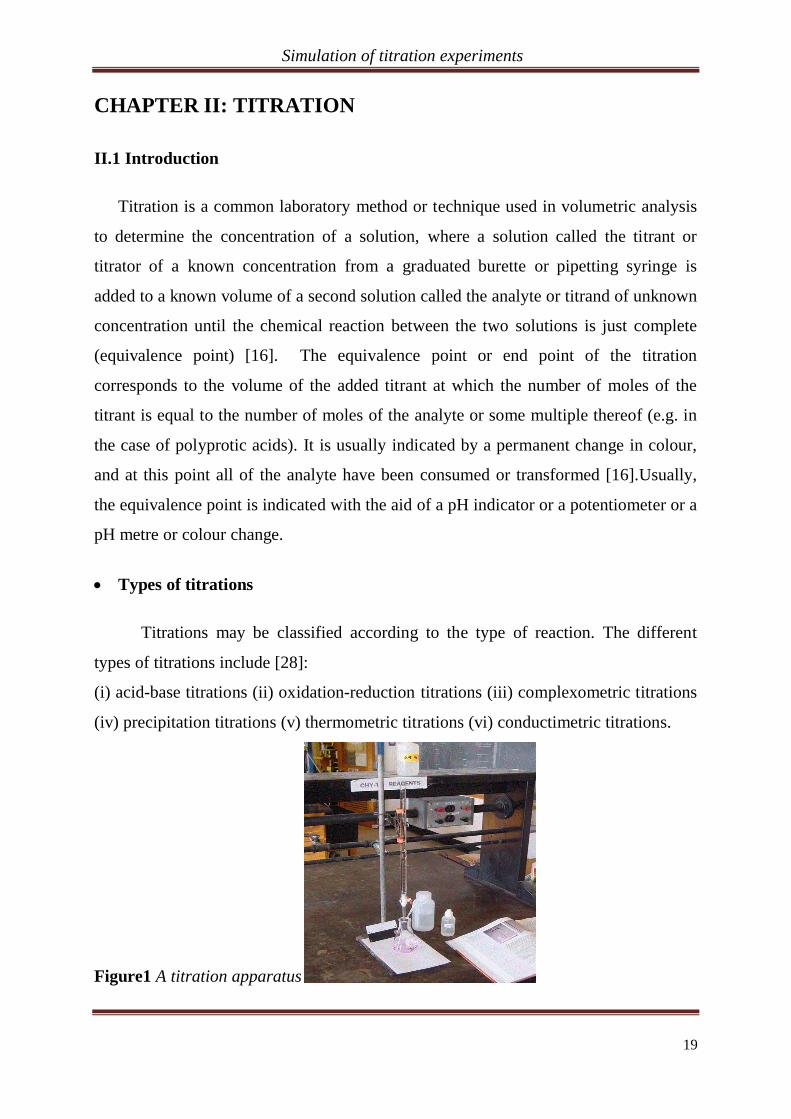
Types of titrations
Titrations may be classified according to the type of reaction. The different
types of titrations include [28]:
(i) acid-base titrations (ii) oxidation-reduction titrations (iii) complexometric titrations
(iv) precipitation titrations (v) thermometric titrations (vi) conductimetric titrations.
Figure1 A titration apparatus
Simulation of titration experiments
20
Titration procedure
(i)Rinse all glass wares with distilled water.
(ii)Clamp a 50mL burette and fill it with the titrant to a convenient volume.
(iii)Using a 25ml pipette, transfer 25ml for instance, of the analyte into an Erlenmeyer
(conical) flask and place the flask on a white sheet of paper underneath the clamped
burette.
(iv)Where necessary, add two to three drops of an indicator to the content of the
conical flask.
(v)Run the titrant slowly from the burette into the Erlenmeyer flask, while swirling
until the end point is reached. This is the approximate titration.
(vi)Carry out two more accurate titrations and record your results in a table [17].
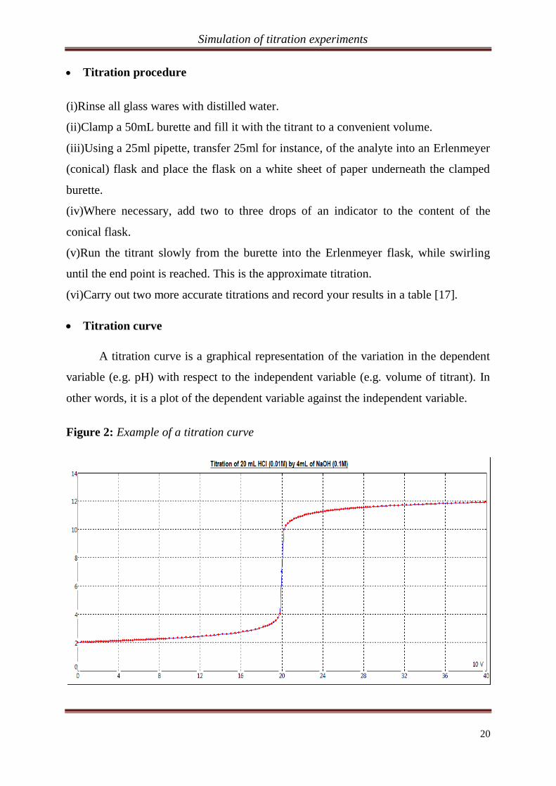
Titration curve
A titration curve is a graphical representation of the variation in the dependent
variable (e.g. pH) with respect to the independent variable (e.g. volume of titrant). In
other words, it is a plot of the dependent variable against the independent variable.
Figure 2: Example of a titration curve
Simulation of titration experiments
21
II.2 Acid-base titrations
Acid-base titrations are based on the neutralization reaction of an acid by a base
and vice-versa [16]. Acid-base titrations can be grouped under the following headings:
Titration of a strong acid with a strong base, titration of a strong acid with a weak
base, titration of a weak acid with a strong base, titration of a weak acid with a weak
base. During an acid-base titration, the number of moles of the analyte diminishes
gradually and there is a change in pH as the titrant is added. The change in pH depends
largely on the strengths of the acid and base used [16].
The end point of an acid-base titration
The end point of an acid-base titration is the point at which a single drop of the
titrant causes an immediate change in the indicator colour. At this point, the number of
moles of the acid is equal to the number of moles of the base [16].
In the classic strong acid-strong base titration, the end point is the point at which the
pH of the analyte (acid or base) is just about equal to 7 [17].
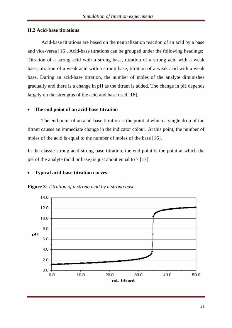
Typical acid-base titration curves
Figure 3: Titration of a strong acid by a strong base.
Simulation of titration experiments
22
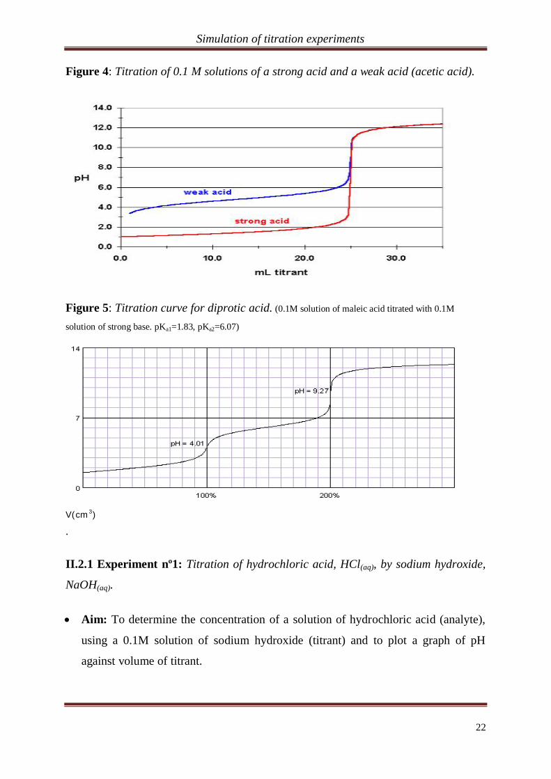
Figure 4: Titration of 0.1 M solutions of a strong acid and a weak acid (acetic acid).
Figure 5: Titration curve for diprotic acid. (0.1M solution of maleic acid titrated with 0.1M
solution of strong base. pKa1=1.83, pKa2=6.07)
V(cm3)
.
II.2.1 Experiment nº1: Titration of hydrochloric acid, HCl(aq), by sodium hydroxide,
NaOH(aq).
Aim: To determine the concentration of a solution of hydrochloric acid (analyte),
using a 0.1M solution of sodium hydroxide (titrant) and to plot a graph of pH
against volume of titrant.
Simulation of titration experiments
23
Requirements: 25cm3 pipette, 50cm3 burette, 250cm3 conical flask, 250cm3
beakers, bromothymol blue indicator, 0.1MNaOH(aq), HCl(aq) solution, clamp and
stand, white sheet of paper.
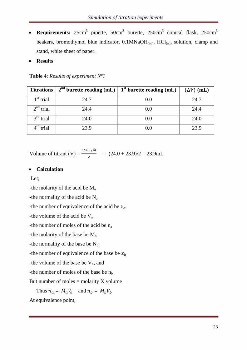
Results
Table 4: Results of experiment Nº1
Titrations 2nd burette reading (mL) 1st burette reading (mL) ( ) (mL)
1st trial 24.7 0.0 24.7
2nd trial 24.4 0.0 24.4
3rd trial 24.0 0.0 24.0
4th trial 23.9 0.0 23.9
Volume of titrant (V) = = (24.0 + 23.9)/2 = 23.9mL
Calculation
Let;
-the molarity of the acid be Ma
-the normality of the acid be Na
-the number of equivalence of the acid be
-the volume of the acid be Va
-the number of moles of the acid be na
-the molarity of the base be Mb
-the normality of the base be Nb
-the number of equivalence of the base be
-the volume of the base be Vb, and
-the number of moles of the base be nb
But number of moles = molarity X volume
Thus = and =
At equivalence point,
Simulation of titration experiments
24
The number of equivalent gram of acid = the number of equivalent gram of base
that is =
But Ma = Na and Mb = Nb , therefore =
Or =
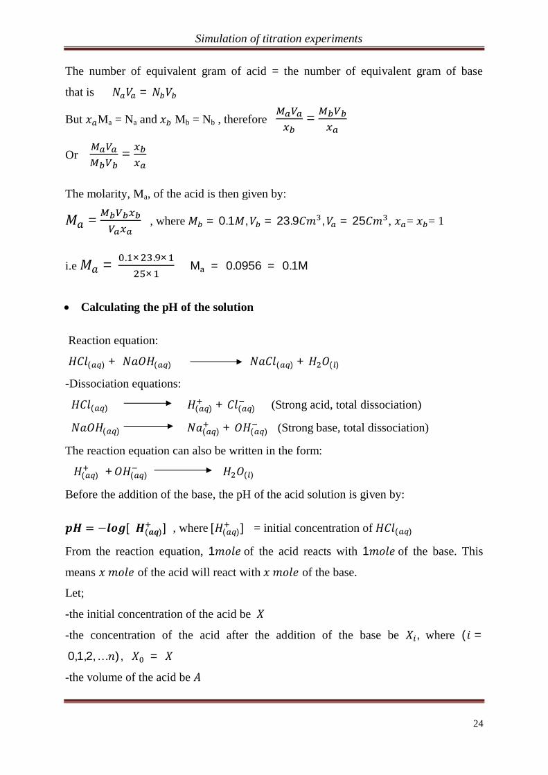
The molarity, Ma, of the acid is then given by:
= , where = 0.1 , = 23.9 , = 25 , = = 1
i.e = . × . ××
M = 0.0956 = 0.1M
Calculating the pH of the solution
Reaction equation:
( ) + ( ) ( ) + ( )
-Dissociation equations:
( ) ( ) + ( ) (Strong acid, total dissociation)
( ) ( ) + ( ) (Strong base, total dissociation)
The reaction equation can also be written in the form:
( ) + ( ) ( )
Before the addition of the base, the pH of the acid solution is given by:
[ ( )] , where [ ( )] = initial concentration of ( )
From the reaction equation, 1 of the acid reacts with 1 of the base. This
means of the acid will react with of the base.
Let;
-the initial concentration of the acid be
-the concentration of the acid after the addition of the base be , where ( =
0,1,2, … ), =
-the volume of the acid be
Simulation of titration experiments
25
-the concentration of the base be
-the volume of the base added be , = 0,1 2, … = 0
It follows that, the concentration of the acid, Xi, after the addition of a volume, Vi, of
the base is given by: = ( – )/( + ).
Therefore the pH of the resulting solution is given by:
= [( – )/( + )], > .
If AX< CVi (after the equivalence point, when the resulting solution becomes basic),
the pH of the solution is then given by: = 14 + [( – )/( + )].
-At the equivalence point, where = , the pH of the resulting solution is
approximately equal to 7.0. this corresponds to the end point pH of bromothymol blue.
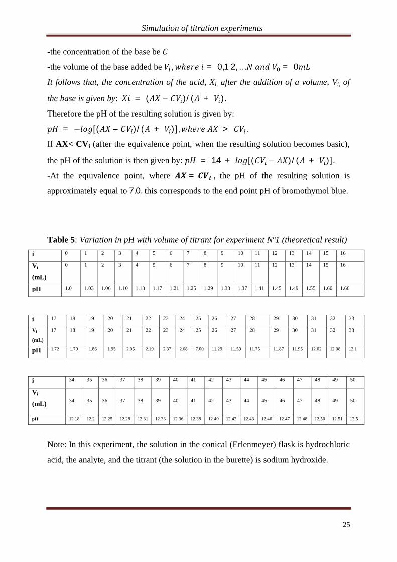
Table 5: Variation in pH with volume of titrant for experiment Nº1 (theoretical result) i 0 1 2 3 4 5 6 7 8 9 10 11 12 13 14 15 16
Vi
(mL)
0 1 2 3 4 5 6 7 8 9 10 11 12 13 14 15 16
pH 1.0 1.03 1.06 1.10 1.13 1.17 1.21 1.25 1.29 1.33 1.37 1.41 1.45 1.49 1.55 1.60 1.66
i 17 18 19 20 21 22 23 24 25 26 27 28 29 30 31 32 33
Vi
(mL)
17 18 19 20 21 22 23 24 25 26 27 28 29 30 31 32 33
pH 1.72 1.79 1.86 1.95 2.05 2.19 2.37 2.68 7.00 11.29 11.59 11.75 11.87 11.95 12.02 12.08 12.1
i 34 35 36 37 38 39 40 41 42 43 44 45 46 47 48 49 50
Vi
(mL)
34
35
36
37
38
39
40
41
42
43
44
45
46
47
48
49
50
pH 12.18 12.2 12.25 12.28 12.31 12.33 12.36 12.38 12.40 12.42 12.43 12.46 12.47 12.48 12.50 12.51 12.5
Note: In this experiment, the solution in the conical (Erlenmeyer) flask is hydrochloric
acid, the analyte, and the titrant (the solution in the burette) is sodium hydroxide.
Simulation of titration experiments
26
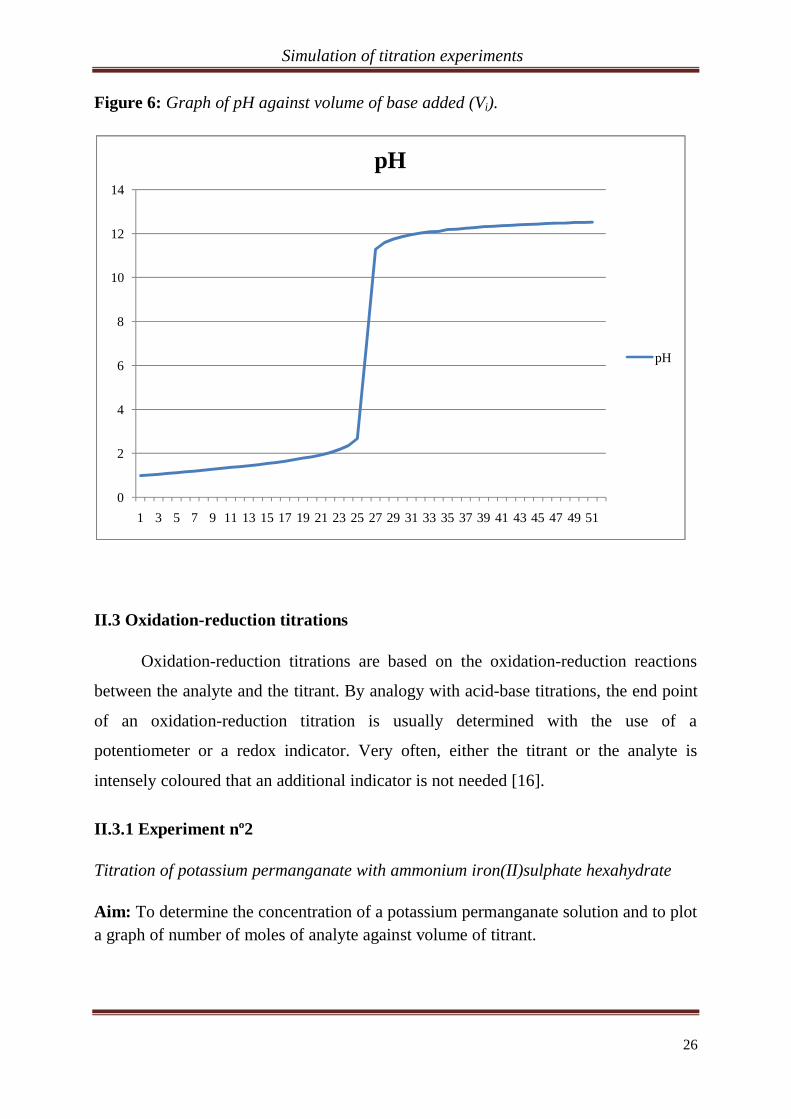
Figure 6: Graph of pH against volume of base added (Vi).
II.3 Oxidation-reduction titrations
Oxidation-reduction titrations are based on the oxidation-reduction reactions
between the analyte and the titrant. By analogy with acid-base titrations, the end point
of an oxidation-reduction titration is usually determined with the use of a
potentiometer or a redox indicator. Very often, either the titrant or the analyte is
intensely coloured that an additional indicator is not needed [16].
II.3.1 Experiment nº2
Titration of potassium permanganate with ammonium iron(II)sulphate hexahydrate
Aim: To determine the concentration of a potassium permanganate solution and to plot a graph of number of moles of analyte against volume of titrant.
0
2
4
6
8
10
12
14
1 3 5 7 9 11 13 15 17 19 21 23 25 27 29 31 33 35 37 39 41 43 45 47 49 51
pH
pH

Simulation of titration experiments
27
Requirements
Potassium permanganate solution, ammonium iron(II)sulphate solution, dilute
sulphuric acid and usual titration equipments.
Procedure
1) Weigh accurately 14.70g of ( ) ( )2.6H2O(s), dissolve and transfer into a
250mL volumetric flask. Complete the solution up to the 250 mark with distilled
water. Stopper and swirl the flask well to homogenize the solution.
2) Rinse and fill a 50mL burette with the potassium permanganate solution previously
prepared.
3) Using a clean and suitably rinsed pipette, place 25 of ammonium
iron(II)sulphate hexahydrate in a 250 Erlenmeyer flask, add 25 of dilute
sulphuric acid, shake and titrate with the permanganate solution until the first
permanent pale pink colour is obtained. Do four titrations and record the results in the
table below.
Table 6: Results of experiment Nº2
Titrations 2nd burette reading (mL) 1st burette reading (mL) (mL)
1st trial 15.9 0.0 15.9
2nd trial 15.7 0.0 15.7
3rd trial 15.5 0.0 15.5
4th trial 15.5 0.0 15.5
volume of titrant = = . . = 15.5mL
Equations:
( ) + 8 ( ) + 5 ( ) + 4 ( ) (Reduction)
( ) ( ) + + e- (oxidation)
Overall equation:
( ) + 5 ( ) + 8 ( ) ( ) + ( ) + 4 ( )
Simulation of titration experiments
28
Calculations:
Let;
-the normality of ( )) be N1 and the concentration be C1
-the volume of ( ) be V1
-the number of equivalence of ( ) be
-the number of moles of ( ) be n1
-the concentration of ( )be C2 and the normality be N2
-the volume of ( )be V2
-the number of equivalence of ( ) be
-the number of moles of ( ) be n2, where n1 and n2 are the stoichiometric
coefficients in the balanced equation.
It follows that; n1 = C1V1 and n2= C2V2
At equivalence point, the number of equivalent gram of the oxidant is equal to the
number of equivalent gram of the reductant. That is; N1V1 = N2V2
But = and =
It follows that = , or =
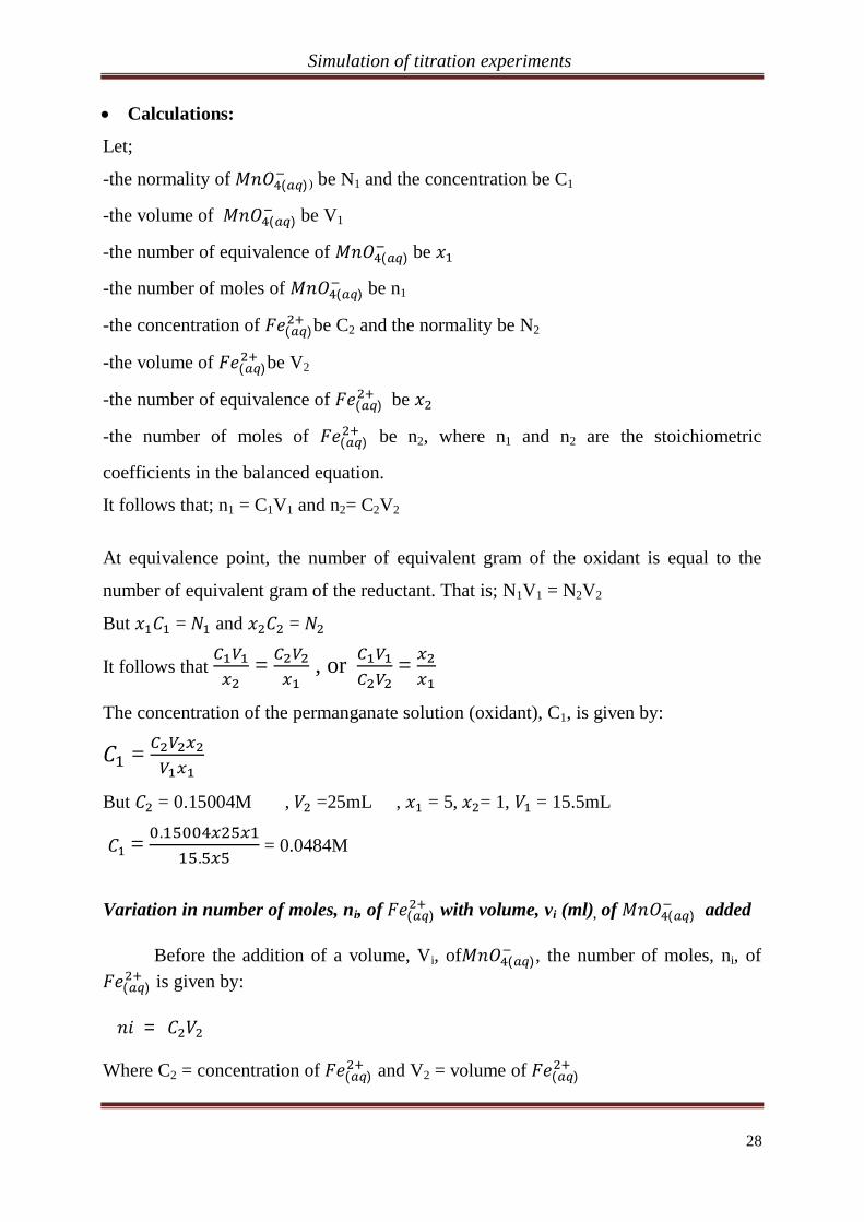
The concentration of the permanganate solution (oxidant), C1, is given by:
=
But = 0.15004M , =25mL , = 5, = 1, = 15.5mL
= ..
= 0.0484M
Variation in number of moles, ni, of ( ) with volume, vi (ml), of ( ) added
Before the addition of a volume, Vi, of ( ), the number of moles, ni, of ( ) is given by:
=
Where C2 = concentration of ( ) and V2 = volume of ( )
Simulation of titration experiments
29
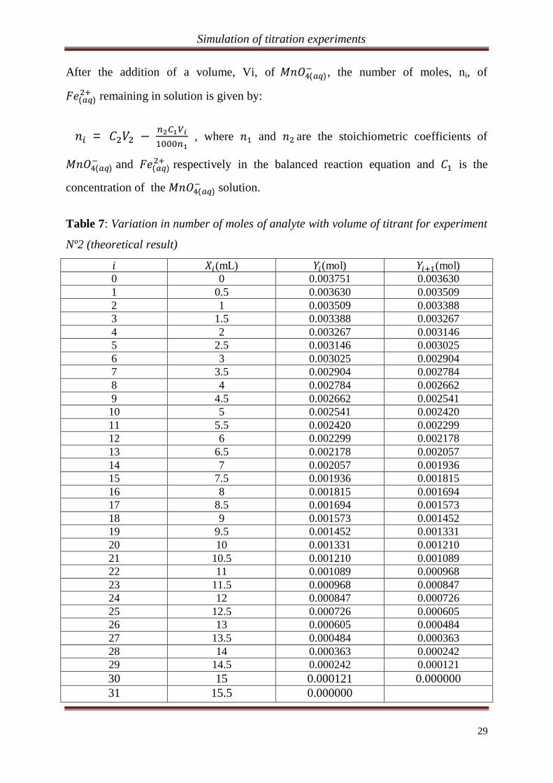
After the addition of a volume, Vi, of ( ), the number of moles, ni, of
( ) remaining in solution is given by:
= , where and are the stoichiometric coefficients of
( ) and ( ) respectively in the balanced reaction equation and is the
concentration of the ( ) solution.
Table 7: Variation in number of moles of analyte with volume of titrant for experiment
Nº2 (theoretical result)
(mL) (mol) (mol) 0 0 0.003751 0.003630 1 0.5 0.003630 0.003509 2 1 0.003509 0.003388 3 1.5 0.003388 0.003267 4 2 0.003267 0.003146 5 2.5 0.003146 0.003025 6 3 0.003025 0.002904 7 3.5 0.002904 0.002784 8 4 0.002784 0.002662 9 4.5 0.002662 0.002541 10 5 0.002541 0.002420 11 5.5 0.002420 0.002299 12 6 0.002299 0.002178 13 6.5 0.002178 0.002057 14 7 0.002057 0.001936 15 7.5 0.001936 0.001815 16 8 0.001815 0.001694 17 8.5 0.001694 0.001573 18 9 0.001573 0.001452 19 9.5 0.001452 0.001331 20 10 0.001331 0.001210 21 10.5 0.001210 0.001089 22 11 0.001089 0.000968 23 11.5 0.000968 0.000847 24 12 0.000847 0.000726 25 12.5 0.000726 0.000605 26 13 0.000605 0.000484 27 13.5 0.000484 0.000363 28 14 0.000363 0.000242 29 14.5 0.000242 0.000121 30 15 0.000121 0.000000 31 15.5 0.000000
Simulation of titration experiments
30
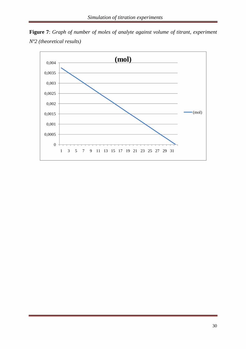
Figure 7: Graph of number of moles of analyte against volume of titrant, experiment
Nº2 (theoretical results)
0
0,0005
0,001
0,0015
0,002
0,0025
0,003
0,0035
0,004
1 3 5 7 9 11 13 15 17 19 21 23 25 27 29 31
(mol)
(mol)
Simulation of titration experiments
31
CHAPTER III: NUMERICAL METHODS AND SIMULATION
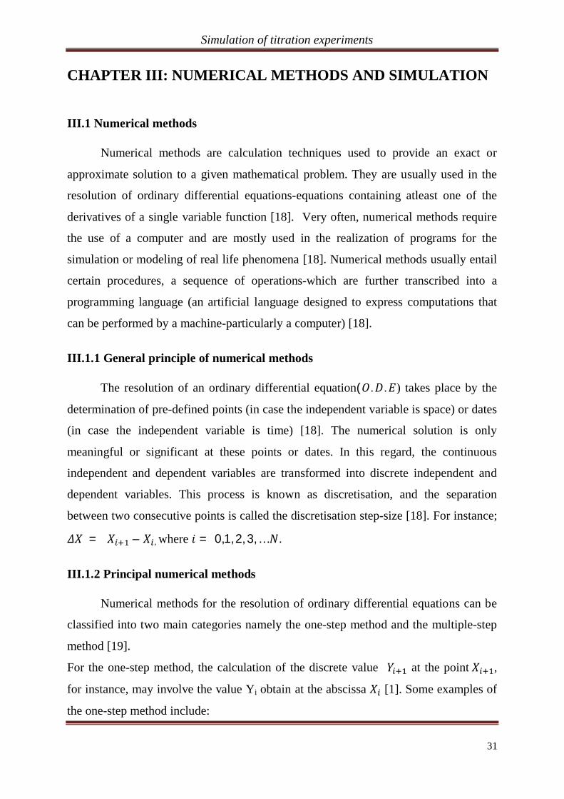
III.1 Numerical methods
Numerical methods are calculation techniques used to provide an exact or
approximate solution to a given mathematical problem. They are usually used in the
resolution of ordinary differential equations-equations containing atleast one of the
derivatives of a single variable function [18]. Very often, numerical methods require
the use of a computer and are mostly used in the realization of programs for the
simulation or modeling of real life phenomena [18]. Numerical methods usually entail
certain procedures, a sequence of operations-which are further transcribed into a
programming language (an artificial language designed to express computations that
can be performed by a machine-particularly a computer) [18].
III.1.1 General principle of numerical methods
The resolution of an ordinary differential equation( . . ) takes place by the
determination of pre-defined points (in case the independent variable is space) or dates
(in case the independent variable is time) [18]. The numerical solution is only
meaningful or significant at these points or dates. In this regard, the continuous
independent and dependent variables are transformed into discrete independent and
dependent variables. This process is known as discretisation, and the separation
between two consecutive points is called the discretisation step-size [18]. For instance;
= – , where = 0,1, 2, 3, … .
III.1.2 Principal numerical methods
Numerical methods for the resolution of ordinary differential equations can be
classified into two main categories namely the one-step method and the multiple-step
method [19].
For the one-step method, the calculation of the discrete value at the point ,
for instance, may involve the value Yi obtain at the abscissa [1]. Some examples of
the one-step method include:

Simulation of titration experiments
32
Euler explicit method
This is an iterative method, where the value of the dependent variable is
determined or obtained by adding the change, , to the value of . If h is the
discretisation step-size at (i.e. = ), then the Euler explicit method is
defined as follows:
-definition of the independent variable,
Initial value:
Recurrence relation:
=
Evaluation of the dependent variable .
Initial value:
Recurrence relation:
= ( , )
Note: This method-which is the simplest of all numerical methods, is said to be
explicit because the quantity is entirely or explicitly expressed as a function of
Also, ( , ) is the gradient
of the tangent line to the curve.
Euler implicit method
It is defined by:
=
= ( , )
Simulation of titration experiments
33
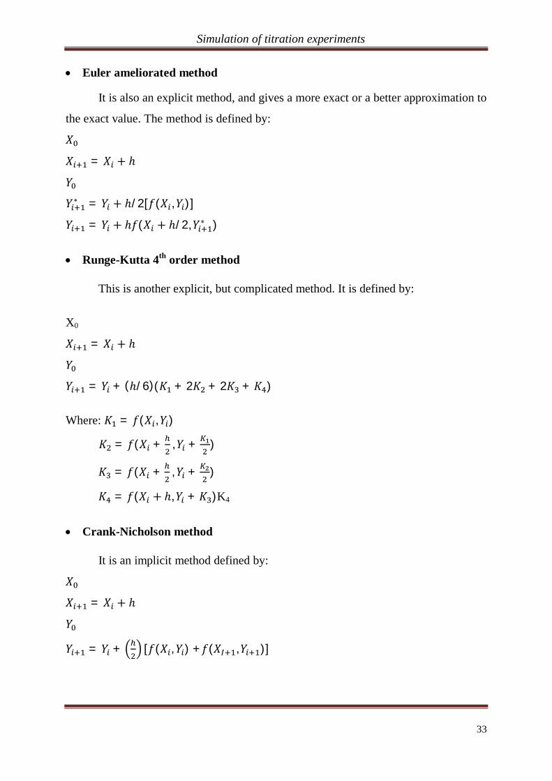
Euler ameliorated method
It is also an explicit method, and gives a more exact or a better approximation to
the exact value. The method is defined by:
=
= /2[ ( , )]
= ( /2, )
Runge-Kutta 4th order method
This is another explicit, but complicated method. It is defined by:
X0
=
= + ( /6)( + 2 + 2 + )
Where: = ( , )
= ( + , + )
= ( + , + )
= ( , + )K4
Crank-Nicholson method
It is an implicit method defined by:
=
= + [ ( , ) + ( , )]
Simulation of titration experiments
34
III.2 Simulation
III.2.1 Definitions
According to Oxford Advanced Learner’s dictionary 6th edition, simulation is a
situation in which a particular set of conditions is created artificially in order to study
or experience something that could exist in reality.
According to the free dictionary [20]; simulation is the act of imitating the behavior of
some situation or some process by means of something suitably analogous (especially
for the purpose of study or personnel training).
Simulation, in computer science, is the technique of representing the real world by a
computer program; “a simulation should imitate the internal processes and not merely
the results of the thing being simulated”.
A computer program (also called a software program or just a program) is a sequence
of instructions written to perform a specific task for a computer.
Computer programming is the iterative process of writing or editing (i.e. testing,
analyzing, and refining, and sometimes coordinating with other programmers on
jointly developed program) source code.
Source code in computer science is any collection of statements or declarations written
in some human readable computer programming language. It is usually used by
programmers to specify the actions to be performed by a computer.
A programming language is an artificial language or a notation for writing programs,
which are specifications of an algorithm or a computation.
An algorithm (also called organigram) is a list of well defined instructions for
completing a task. In other words, it is an effective method for solving a problem as a
finite sequence of steps. Algorithms are usually used for calculation, data processing,
automated reasoning and many other fields.
Simulation of titration experiments
35
III.2.2 Simulation of an acid-base titration
III.2.2.1 principle of acid-base titration simulation
The following points should be noted when simulating an acid-base
titration[20]:
1) Choose either an acid or a base solution to put in the conical flask and decide the
concentration and the volume of the solution.
2) Select a standard reagent to fill the burette. If you have chosen an acid solution for
the conical flask in step 1, you should choose a base solution for the burette and vice
versa. The volume of the solution in the burette should be more than that in the conical
flask.
3) Choose an appropriate indicator for the titration and proceed with the virtual
titration.
4) View your titration curve from your data.
III.2.2.2 Application example
Simulation of the titration of hydrochloric acid ( ( )) by sodium hydroxide
( ( )))
Reaction equation: ( ) + ( ) ( ) + ( )
Let;
- The titrant be sodium hydroxide, ( ) in the burette
- The analyte be hydrochloric acid, ( ) in the conical flask
- The initial concentration of hydrochloric acid, ( ), be = 0.1
- The volume of hydrochloric acid, ( ), be = 25
- The number of moles of hydrochloric acid, ( ), be = 1
- The concentration of sodium hydroxide, ( ), be = 0.1
- The volume of sodium hydroxide, ( ), be = 50
Simulation of titration experiments
36
- The number of moles of sodium hydroxide, ( ), be = 1
- The indicator be bromothymol blue
- The endpoint pH of bromothymol blue be P, P = 7.0000
- The colour of bromothymol blue be yellow in the acid medium and blue in the basic
medium.
It follows that the variation in the pH of the solution before the equivalence point, ,
is given by the ordinary differential equation:
= ( + )/( )( + ). Where (0) = 1.0000, > and A is a
positive constant, = 0.434
Also, after the equivalence point, where > , the variation in the , , of the
resulting solution is given by the following ordinary differential equation:
= ( + )/( )( + ); (0) = 1.0000 Y(0)
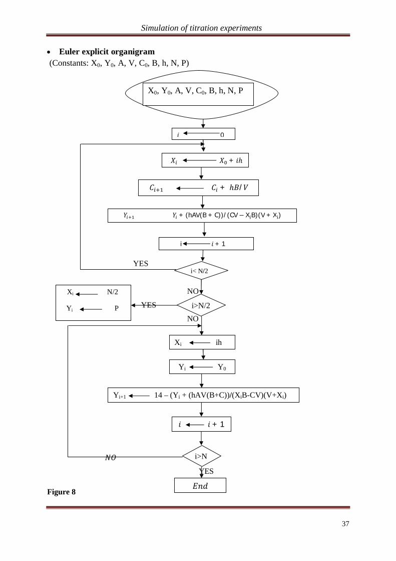
Euler explicit algorithm
Let the discretisation step-size be h = 1, and = 0, 1, 2, 3, . . . , ; = 50
The Euler explicit algorithm before the equivalence point is given by:
=
= + ( ( + ))/( )( + )
After the equivalence point, where < , the Euler explicit algorithm is given by:
=
= 14 ( + ( ( + ))/( )( + )
Simulation of titration experiments
37
Euler explicit organigram (Constants: X0, Y0, A, V, C0, B, h, N, P)
YES
NO
YES
NO
YES
Figure 8
X0, Y0, A, V, C, B, h, N, P
0
+
+ (hAV(B + C))/(CV X B)(V + X )
i + 1
i< N/2
i>N/2
Xi N/2
Yi P
Xi ih
Yi Y0
Yi+1 14 – (Yi + (hAV(B+C))/(XiB-CV)(V+Xi)
i>N
+ 1
X0, Y0, A, V, C0, B, h, N, P
+ /
Simulation of titration experiments
38
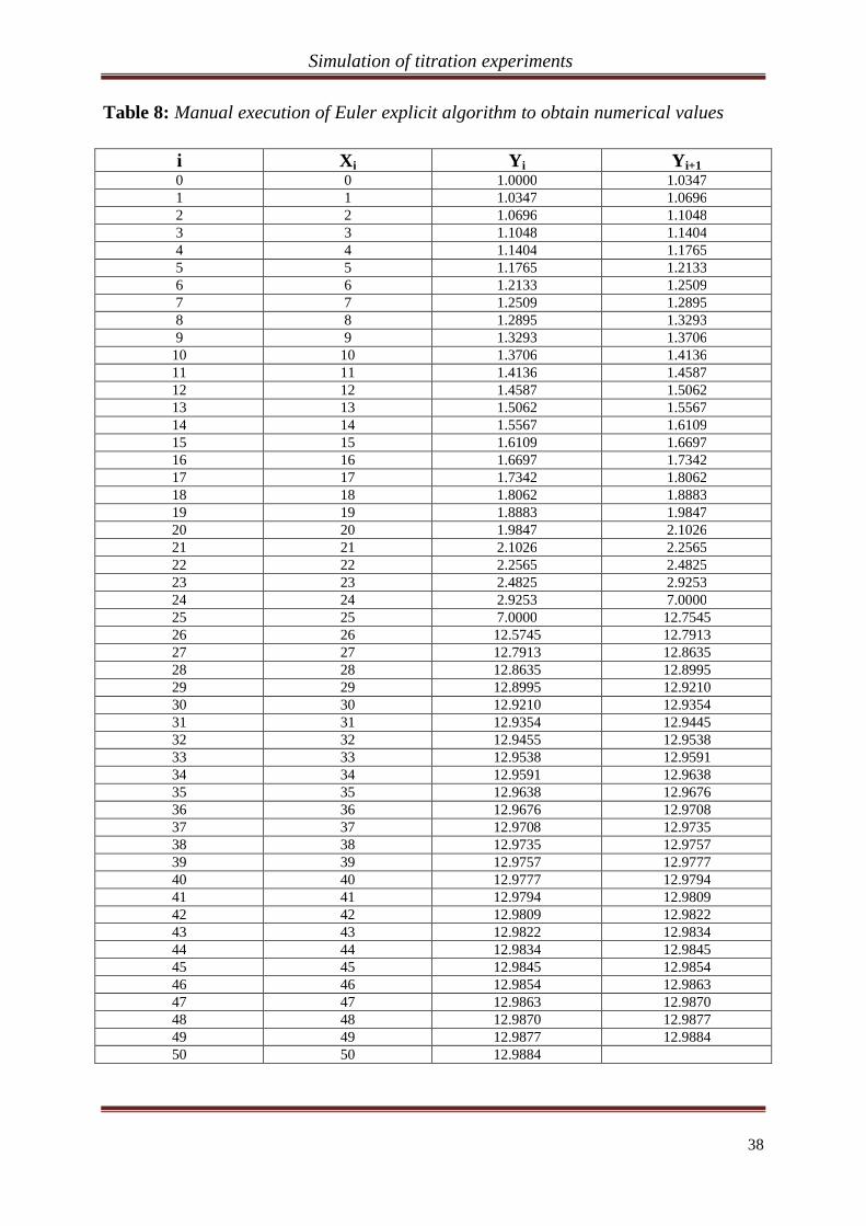
Table 8: Manual execution of Euler explicit algorithm to obtain numerical values
i Xi Yi Yi+1 0 0 1.0000 1.0347 1 1 1.0347 1.0696 2 2 1.0696 1.1048 3 3 1.1048 1.1404 4 4 1.1404 1.1765 5 5 1.1765 1.2133 6 6 1.2133 1.2509 7 7 1.2509 1.2895 8 8 1.2895 1.3293 9 9 1.3293 1.3706
10 10 1.3706 1.4136 11 11 1.4136 1.4587 12 12 1.4587 1.5062 13 13 1.5062 1.5567 14 14 1.5567 1.6109 15 15 1.6109 1.6697 16 16 1.6697 1.7342 17 17 1.7342 1.8062 18 18 1.8062 1.8883 19 19 1.8883 1.9847 20 20 1.9847 2.1026 21 21 2.1026 2.2565 22 22 2.2565 2.4825 23 23 2.4825 2.9253 24 24 2.9253 7.0000 25 25 7.0000 12.7545 26 26 12.5745 12.7913 27 27 12.7913 12.8635 28 28 12.8635 12.8995 29 29 12.8995 12.9210 30 30 12.9210 12.9354 31 31 12.9354 12.9445 32 32 12.9455 12.9538 33 33 12.9538 12.9591 34 34 12.9591 12.9638 35 35 12.9638 12.9676 36 36 12.9676 12.9708 37 37 12.9708 12.9735 38 38 12.9735 12.9757 39 39 12.9757 12.9777 40 40 12.9777 12.9794 41 41 12.9794 12.9809 42 42 12.9809 12.9822 43 43 12.9822 12.9834 44 44 12.9834 12.9845 45 45 12.9845 12.9854 46 46 12.9854 12.9863 47 47 12.9863 12.9870 48 48 12.9870 12.9877 49 49 12.9877 12.9884 50 50 12.9884
Simulation of titration experiments
39
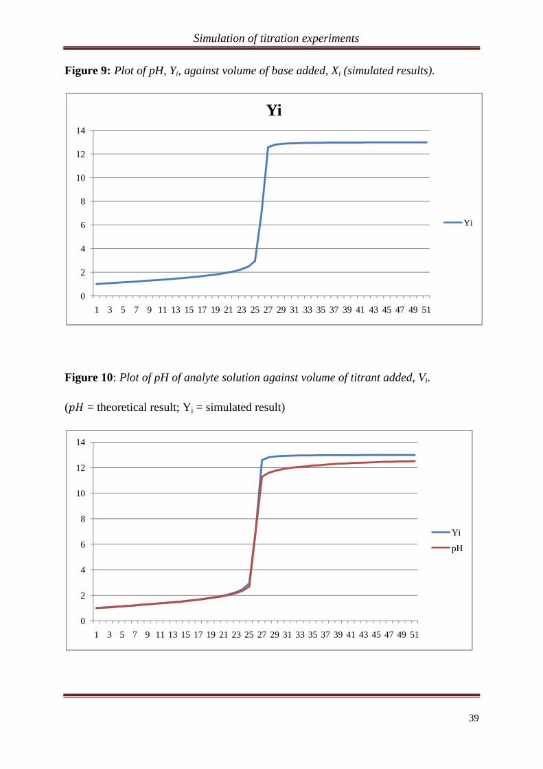
Figure 9: Plot of pH, Yi, against volume of base added, Xi (simulated results).
Figure 10: Plot of pH of analyte solution against volume of titrant added, Vi.
( = theoretical result; Yi = simulated result)
0
2
4
6
8
10
12
14
1 3 5 7 9 11 13 15 17 19 21 23 25 27 29 31 33 35 37 39 41 43 45 47 49 51
Yi
Yi
0
2
4
6
8
10
12
14
1 3 5 7 9 11 13 15 17 19 21 23 25 27 29 31 33 35 37 39 41 43 45 47 49 51
Yi
pH
Simulation of titration experiments
40
III.2.3 Simulation of an oxidation-reduction titration
III.2.3.1 Principle of simulation of an oxidation-reduction titration
The following points should be noted when simulating an oxidation-reduction
titration [20]:
1) Choose either an oxidant or a reductant solution to put in the conical flask and
decide the concentration and the volume of the solution.
2) Select a standard reagent to fill the burette. If you have chosen an oxidant solution
for the conical flask in step 1, you should choose a reductant solution for the burette
and vice versa. The volume of the solution in the burette should be more than that in
the conical flask.
3) If necessary, choose an appropriate indicator for the titration and proceed with the
simulation.
4) View your titration curve from your data.
III.2.3.2 Application example
Simulation of the titration of ( )ions, analyte, with ( ) ions, titrant.
Reaction equations:
( ) + 8 ( ) + 5 + ( ) + 4 ( ) (reduction)
( ) ( ) + (Oxidation)
Overall equation:
( ) + 5 ( ) + 8 ( ) ( ) + 5 ( ) + 4 ( )
Let;
- The stoichiometric coefficients of ( ) and ( )in the balanced equation be
and respectively
- The concentration of ( )be and the volume be ( = 0, 1, 2, … , ),
where N is an integer.
Simulation of titration experiments
41
- The concentration of ( ) be and the volume be
- The number of moles of ( ) , = 0, 1, 2, …
- The discretisation step-size be
Where = 31, = 1, = 5, = 0.0484 / , = 0 , = 0.15004 / ,
=25 10 , h = 0.5, = 0.003751 .
The variation in the number of moles , of ( ) with volume of ( ) added, ,
is given by the relation:
= , (0) = = 0.003751 (initial number of moles of ( ),
analyte)
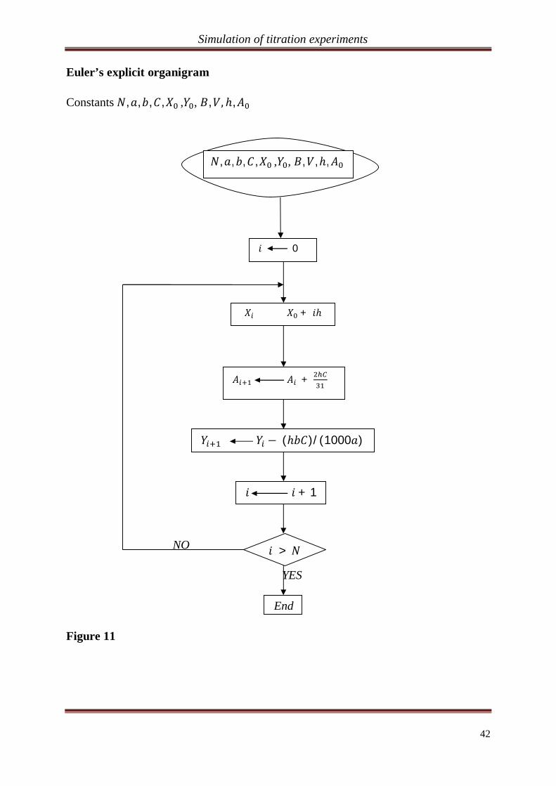
Euler’s explicit algorithm
= +
= -
Simulation of titration experiments
42
Euler’s explicit organigram
Constants , , , , , , , ,
NO
YES
Figure 11
, , , , , , , , ,
0
+
+
( )/(1000 )
+ 1
>
End
Simulation of titration experiments
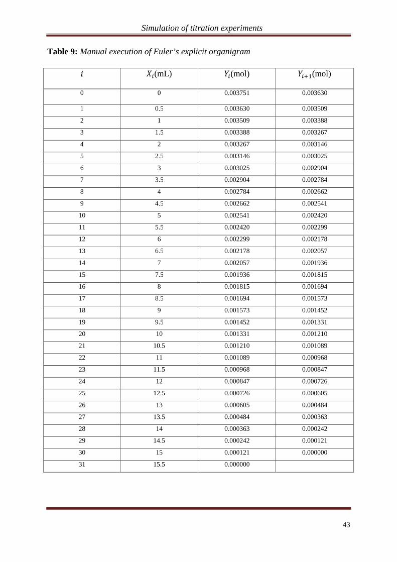
43
Table 9: Manual execution of Euler’s explicit organigram
(mL) (mol) (mol)
0 0 0.003751 0.003630
1 0.5 0.003630 0.003509
2 1 0.003509 0.003388
3 1.5 0.003388 0.003267
4 2 0.003267 0.003146
5 2.5 0.003146 0.003025
6 3 0.003025 0.002904
7 3.5 0.002904 0.002784
8 4 0.002784 0.002662
9 4.5 0.002662 0.002541
10 5 0.002541 0.002420
11 5.5 0.002420 0.002299
12 6 0.002299 0.002178
13 6.5 0.002178 0.002057
14 7 0.002057 0.001936
15 7.5 0.001936 0.001815
16 8 0.001815 0.001694
17 8.5 0.001694 0.001573
18 9 0.001573 0.001452
19 9.5 0.001452 0.001331
20 10 0.001331 0.001210
21 10.5 0.001210 0.001089
22 11 0.001089 0.000968
23 11.5 0.000968 0.000847
24 12 0.000847 0.000726
25 12.5 0.000726 0.000605
26 13 0.000605 0.000484
27 13.5 0.000484 0.000363
28 14 0.000363 0.000242
29 14.5 0.000242 0.000121
30 15 0.000121 0.000000
31 15.5 0.000000
Simulation of titration experiments
44
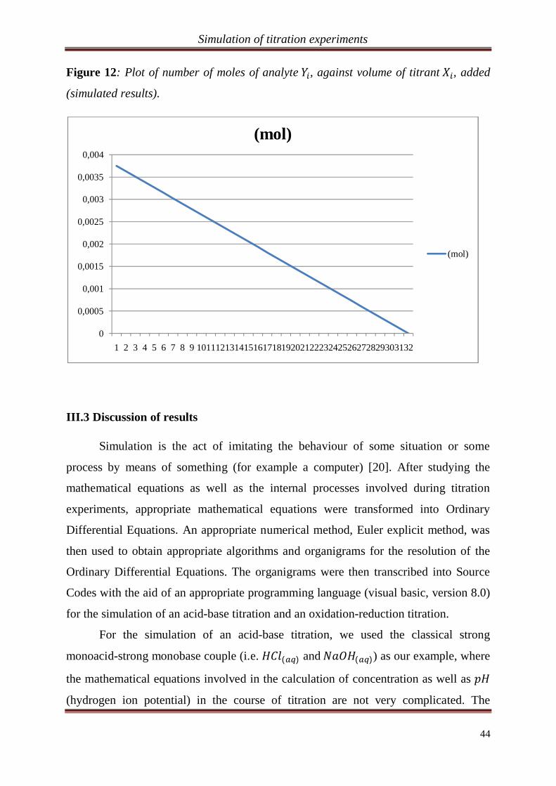
Figure 12: Plot of number of moles of analyte , against volume of titrant , added
(simulated results).
III.3 Discussion of results
Simulation is the act of imitating the behaviour of some situation or some
process by means of something (for example a computer) [20]. After studying the
mathematical equations as well as the internal processes involved during titration
experiments, appropriate mathematical equations were transformed into Ordinary
Differential Equations. An appropriate numerical method, Euler explicit method, was
then used to obtain appropriate algorithms and organigrams for the resolution of the
Ordinary Differential Equations. The organigrams were then transcribed into Source
Codes with the aid of an appropriate programming language (visual basic, version 8.0)
for the simulation of an acid-base titration and an oxidation-reduction titration.
For the simulation of an acid-base titration, we used the classical strong
monoacid-strong monobase couple (i.e. ( ) and ( )) as our example, where
the mathematical equations involved in the calculation of concentration as well as
(hydrogen ion potential) in the course of titration are not very complicated. The
0
0,0005
0,001
0,0015
0,002
0,0025
0,003
0,0035
0,004
1 2 3 4 5 6 7 8 9 1011121314151617181920212223242526272829303132
(mol)
(mol)
Simulation of titration experiments
45
endpoint indicator used in this example is Bromothymol blue, which produces a
yellow coloration in an acid medium and a blue coloration in a basic medium, with an
endpoint pH of approximately 7.0.
In this example, the titrant is the base, sodium hydroxide ( ( )), in the burette
and the analyte is the acid, hydrochloric acid ( ( )), in the conical flask or
Erlenmeyer. The concentration of the base is 0.1M, while the volume of the acid is
25mL. Before titration, the initial pH of the acid solution, analyte, is 1.0.
In the course of the titration, the pH of the acid solution, analyte, gradually increases
from 1.0 up to 2.9253 after the addition of 24.0mL of the base, titrant, according to the
formula; +1 = ( + )( )( + )
; 0 = 1.0 0 = 0 .
At the equivalence point, after the addition of 25.0mL of the base, titrant, the initial
concentration of the pure acid solution is evaluated at approximately 0.1M, while the
pH of the resulting solution drastically increased to 7.0 and the colour of the solution
changed from yellow to blue. This pH value corresponds to the endpoint pH of
Bromothymol blue, and at this point, the number of moles of the acid and the base are
equal. In other words the reaction between the acid and the base is complete and the
resulting solution is neutral as depicted by the following reaction equation:
( ) + ( ) ( ) + ( )
After the equivalence point, the resulting solution is now purely basic and the rises
steeply from 7.0 to 12.5745, when the volume of the base (titrant) added is 26.0mL.
The of the solution keeps increasing gradually to a final value of 12.9884 after all
of the base (50 ) must have been added according to the formula:
= 14 ( + ( ( + ))/( )( + )
For the simulation of an oxidation-reduction titration, we used the
permanganate ion ( ( )), the oxidant, from an acidified potassium permanganate
( ( )/ ( )) solution as the titrant while the iron(II) ion ( ( )), the reductant,
from ammoniumiron(II) sulphate hexahydrate ( 4) ( 4) . 6 ( ) is the
analyte. Here, we exploited the expression of the number of moles of the analyte as a
function of the volume of the titrant added. The initial concentration of the analyte
Simulation of titration experiments
46
solution, ( ( )), is 0.15004M making a total number of moles of 0.003751mol in a
total volume of 25.0mL. In the course of titration, the number of moles of the analyte,
( ( )), decreases gradually as the titrant, ( ( )), is added down to a final value
of 0.0 , when all of the iron(II) ions, ( ), have been converted into iron(III)
ions, ( ), according to the expression = ; = 0.003751 ,
where a and b are the stoichiometric coefficients of ( )and ( ) respectively
in the balanced reaction equation.
At this point, the concentration of the titrant, MnO ( ), reads approximately 0.0484M,
corresponding to an end point volume of 15.5mL. This is the equivalence point or end
point of the titration process, and it is indicated by a permanent pale pink coloration.
At this point, the number of moles of the analyte is equal to that of the titrant.
A comparison of the theoretical results and the simulated results in both cases
shows that the numerical method used in the construction of the simulator is not only
appropriate, but also simple and efficient given that the results are approximately the
same both for the acid-base titration (0.1 ) and the oxidation-reduction titration
(0.0484 ).
The choice of the numerical method used, Euler explicit method, can be
explained by the fact that it is not only an iterative method; where successive values of
the dependent variable can easily be obtained if the initial value is known, but also the
most simplest explicit method and easy to exploit.
Simulation of titration experiments
47
Conclusion and recommendations
With much readiness, we would say that our work has been very successful.
Very successful in the sense that we were able to attain our objective which was
principally: “to create a software or a simulator that can be used to carry out a
simulation of an acid-base titration and an oxidation-reduction titration”.
To this effect, we were able to carry out a profound study of acid-base titrations and
oxidation-reduction titrations and established all the relevant mathematical equations
involved. We were also able to carry out a review of some of the numerous numerical
methods used in the resolution of Differential Equations in general, from where we
choosed an adequate numerical method (Euler explicit method) used for the
construction of the simulator or software.
Our software or simulator is not only able to simulate the results of an acid-base
titration and an oxidation-reduction titration, but also the internal processes involved.
Computer simulation should not be mistaken with a real life situation. For it is
not because the computer says it is so, that it must be so. Rather, computer simulation
is simply a real life representation based on a theoretical model. For instance, if a
computerized theoretical model is incorrect, then the calculated results would
obviously not be correct, and this may lead to inappropriate or incorrect decisions. As
such a critical analysis of results, the verification of the validity of the theoretical
model used or applied and the confrontation of the forecasted results etc, should be
amongst the reflects that must be uphold as part of the ethics or qualities of the user.
After a critical evaluation of this work, we humbly suggest that this work
should not only serve as a starting point for more research on the simulation of
chemistry practicals in view of coming out with a virtual laboratory, but also that it
should go a long way to encourage the ministry of secondary education, to institute
the use of virtual laboratories in all secondary schools in the country.
Simulation of titration experiments
48
References
1. T. JONG (de) & W.R. VAN JOOLINGEN (1998). Scientific discovery learning
with computer simulations of conceptual domains. Review of Educational Research,
N° 68, p. 168-202.
2. MARIE FARGE (1986). L'approche numérique en physique, Fundamenta
Scientiae pages 155- 175.
3. DURANDEAU, DURUPHTY (2000). Physique-chimie, enseignement de
spécialité, édition Hachette.
4. M.T.H. CHI, J.T. SLOTTA & N. DE LEEUW (1994). From things to processes:
A theory of conceptual change for learning science concepts. Learning
and Instruction, n° 4, p. 27-43.
5. J C GRESSIER (1998). Les acides et les bases-Dunod.
6. Jean-michel MERMET, MATTHIAS OTTO , MIGUEL VALCARCEL , H. M.
WIDMER (2004). Analytical Chemistry (2e édition) Editeur : Wiley.
7. J.M. KETCHA, PEGNYEMB, M.K. NDIKONTAR, A.T. ATCHADE (2005).
Travaux pratiques de chimie générale, édition Paken Page 3-31.
8. C.H. Sorum (1965). Introduction to Semimicro Qualitative Analysis - 3e édition -
Prentice-Hall, Inc.
9. Jean-Louis Brisset , Ahmed Addou , Mustapha Draoui, David Moussa , Fatiha
Abdelmalek (2005). Chimie analytique en solution. Pp240-245. Edition Tec et Doc
10. V. ALEXEEV (1970). Analyse qualitative - Éditions Mir-Moscou.
11. Jacques Mesplède , Jérôme Randon (2004). 100 manipulations de chimie générale
et analytique, 2ème édition- Bréal page 78-124.
12. L. Lopes (Mars 2005). « Réactions "totales" en solution aqueuse », dans Bulletin
de l’union des physiciens, vol. 99, no 872(1), p. 385-396 [ texte intégral ]
13. L. Lopes ; Titrages acidobasiques de mélanges contenant une espèce forte et une
espèce faible : successifs ou simultanés ?
14. John William Hill , Ralph H. Petrucci 22/08/2008 (2e édition). Erpi
15. E. Catherine Housecroft , Alan G. Sharpe 09/09/2010 (3e édition) éditeur De
Boeck
Simulation of titration experiments
49
16. http://en.wikipedia.org/wiki/Titration (01/04/2011; 5:15pm)
17. P.K.Pendong and al; Understanding Chemistry for ordinary level, revised edition
(P.65)
18. http://en.wikipedia.org/wiki/Numerical methods (21/03/2011; 3:30pm)
19. KOZMA R.B. & RUSSEL J. (1997). Multimedia and understanding: expert and
novice responses to different representations of chemical phenomena.
Journal of Research in Science Teaching, vol. 43, n° 9, p. 949-968
20. http://www.the freedictionaty.com/Simulation (16/05/2011; 10:10am)
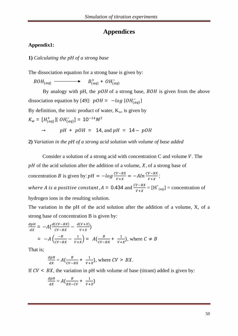
Simulation of titration experiments
50
Appendices
Appendix1:
1) Calculating the pH of a strong base
The dissociation equation for a strong base is given by:
( ) ( ) + ( )
By analogy with pH, the of a strong base, is given from the above
dissociation equation by [49]: = [ ( )]
By definition, the ionic product of water, Kw, is given by
= [ ( )][ ( )] = 10
+ = 14, and = 14 –
2) Variation in the pH of a strong acid solution with volume of base added
Consider a solution of a strong acid with concentration C and volume . The
of the acid solution after the addition of a volume, , of a strong base of
concentration is given by: ;
, = 0.434 and = [H+(aq)] = concentration of
hydrogen ions in the resulting solution.
The variation in the pH of the acid solution after the addition of a volume, X, of a
strong base of concentration B is given by:
= ( ( ) ( ))
= = ( + ), where
That is;
= ( + ), where > .
If < , the variation in pH with volume of base (titrant) added is given by:
= ( + )
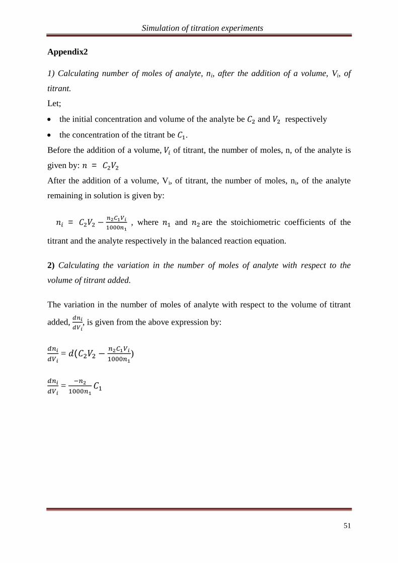
Simulation of titration experiments
51
Appendix2
1) Calculating number of moles of analyte, ni, after the addition of a volume, Vi, of
titrant.
Let;
the initial concentration and volume of the analyte be and respectively
the concentration of the titrant be .
Before the addition of a volume, of titrant, the number of moles, n, of the analyte is
given by: =
After the addition of a volume, Vi, of titrant, the number of moles, ni, of the analyte
remaining in solution is given by:
= , where and are the stoichiometric coefficients of the
titrant and the analyte respectively in the balanced reaction equation.
2) Calculating the variation in the number of moles of analyte with respect to the
volume of titrant added.
The variation in the number of moles of analyte with respect to the volume of titrant
added, , is given from the above expression by:
= ( )
=
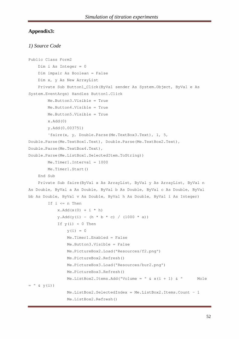
Simulation of titration experiments
52
Appendix3:
1) Source Code
Public Class Form2
Dim i As Integer = 0
Dim impair As Boolean = False
Dim x, y As New ArrayList
Private Sub Button1_Click(ByVal sender As System.Object, ByVal e As
System.EventArgs) Handles Button1.Click
Me.Button3.Visible = True
Me.Button4.Visible = True
Me.Button5.Visible = True
x.Add(0)
y.Add(0.003751)
'faire(x, y, Double.Parse(Me.TextBox3.Text), 1, 5,
Double.Parse(Me.TextBox1.Text), Double.Parse(Me.TextBox2.Text),
Double.Parse(Me.TextBox4.Text),
Double.Parse(Me.ListBox1.SelectedItem.ToString))
Me.Timer1.Interval = 1000
Me.Timer1.Start()
End Sub
Private Sub faire(ByVal x As ArrayList, ByVal y As ArrayList, ByVal n
As Double, ByVal a As Double, ByVal b As Double, ByVal c As Double, ByVal
bb As Double, ByVal v As Double, ByVal h As Double, ByVal i As Integer)
If i <= n Then
x.Add(x(0) + i * h)
y.Add(y(i) - (h * b * c) / (1000 * a))
If y(i) < 0 Then
y(i) = 0
Me.Timer1.Enabled = False
Me.Button3.Visible = False
Me.PictureBox2.Load("Resources/f2.png")
Me.PictureBox2.Refresh()
Me.PictureBox3.Load("Resources/bur2.png")
Me.PictureBox3.Refresh()
Me.ListBox2.Items.Add("Volume = " & x(i + 1) & " Mole
= " & y(i))
Me.ListBox2.SelectedIndex = Me.ListBox2.Items.Count - 1
Me.ListBox2.Refresh()
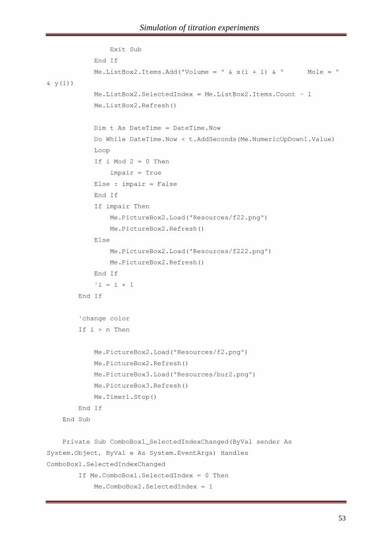
Simulation of titration experiments
53
Exit Sub
End If
Me.ListBox2.Items.Add("Volume = " & x(i + 1) & " Mole = "
& y(i))
Me.ListBox2.SelectedIndex = Me.ListBox2.Items.Count - 1
Me.ListBox2.Refresh()
Dim t As DateTime = DateTime.Now
Do While DateTime.Now < t.AddSeconds(Me.NumericUpDown1.Value)
Loop
If i Mod 2 = 0 Then
impair = True
Else : impair = False
End If
If impair Then
Me.PictureBox2.Load("Resources/f22.png")
Me.PictureBox2.Refresh()
Else
Me.PictureBox2.Load("Resources/f222.png")
Me.PictureBox2.Refresh()
End If
'i = i + 1
End If
'change color
If i > n Then
Me.PictureBox2.Load("Resources/f2.png")
Me.PictureBox2.Refresh()
Me.PictureBox3.Load("Resources/bur2.png")
Me.PictureBox3.Refresh()
Me.Timer1.Stop()
End If
End Sub
Private Sub ComboBox1_SelectedIndexChanged(ByVal sender As
System.Object, ByVal e As System.EventArgs) Handles
ComboBox1.SelectedIndexChanged
If Me.ComboBox1.SelectedIndex = 0 Then
Me.ComboBox2.SelectedIndex = 1
Simulation of titration experiments
54
Me.PictureBox3.Load("Resources/bur1.png")
End If
End Sub
Private Sub ComboBox2_SelectedIndexChanged(ByVal sender As
System.Object, ByVal e As System.EventArgs) Handles
ComboBox2.SelectedIndexChanged
If Me.ComboBox2.SelectedIndex = 1 And
Double.Parse(Me.TextBox4.Text) > 0 Then
Me.ComboBox1.SelectedIndex = 0
Me.PictureBox2.Load("Resources/f1.png")
End If
End Sub
Private Sub Form2_Load(ByVal sender As System.Object, ByVal e As
System.EventArgs) Handles MyBase.Load
'Me.MdiParent = MDIParent1
Me.ListBox1.SelectedIndex = 0
End Sub
Private Sub TextBox1_LostFocus(ByVal sender As Object, ByVal e As
System.EventArgs) Handles TextBox1.LostFocus
Me.TextBox1.Text = Me.TextBox1.Text.Replace(".", ",")
End Sub
Private Sub TextBox2_LostFocus(ByVal sender As Object, ByVal e As
System.EventArgs) Handles TextBox2.LostFocus
Me.TextBox2.Text = Me.TextBox2.Text.Replace(".", ",")
End Sub
Private Sub Timer1_Tick(ByVal sender As System.Object, ByVal e As
System.EventArgs) Handles Timer1.Tick
faire(x, y, Double.Parse(Me.TextBox3.Text), 1, 5,
Double.Parse(Me.TextBox1.Text), Double.Parse(Me.TextBox2.Text),
Double.Parse(Me.TextBox4.Text),
Double.Parse(Me.ListBox1.SelectedItem.ToString()), i)
i = i + 1
End Sub
Simulation of titration experiments
55
Private Sub Button5_Click(ByVal sender As System.Object, ByVal e As
System.EventArgs) Handles Button5.Click
Me.Button3.Visible = False
Me.Button4.Visible = False
Me.Button5.Visible = False
Me.Timer1.Stop()
End Sub
Private Sub Button4_Click(ByVal sender As System.Object, ByVal e As
System.EventArgs) Handles Button4.Click
Me.Button3.Visible = True
Me.Button4.Visible = False
Me.Button5.Visible = True
Me.Timer1.Enabled = True
End Sub
Private Sub Button3_Click(ByVal sender As System.Object, ByVal e As
System.EventArgs) Handles Button3.Click
Me.Button3.Visible = False
Me.Button4.Visible = True
Me.Button5.Visible = True
Me.Timer1.Enabled = False
End Sub
Private Sub Button2_Click(ByVal sender As System.Object, ByVal e As
System.EventArgs) Handles Button2.Click
Me.TextBox1.Text = "0"
Me.TextBox2.Text = "0"
Me.TextBox3.Text = "0"
Me.TextBox4.Text = "0"
Me.ListBox2.Items.Clear()
Me.ListBox2.Refresh()
Me.ComboBox1.Text = ""
Me.ComboBox2.Text = ""
Me.ToolStripStatusLabel1.Text = ""
End Sub
End Class
Imports System.Threading
Simulation of titration experiments
56
Public Class Form1
Private i As Integer = 0
Private first As Boolean = True
Private couleur As Color
Private arret As Boolean = False
Private impair As Boolean = True
Dim x, y As New ArrayList
Dim signal As Boolean = True
Private Sub ComboBox1_SelectedIndexChanged(ByVal sender As
System.Object, ByVal e As System.EventArgs) Handles
ComboBox1.SelectedIndexChanged
If Me.TextBox1.Text = "" And Me.TextBox3.Text = "" Then
Exit Sub
End If
If Me.ComboBox1.SelectedIndex = 0 Then
Me.ComboBox2.SelectedIndex = 1
Me.Label12.Text = "Base"
Me.Label13.Text = "Acid"
Me.PictureBox3.Image = My.Resources.burette1
Else
Me.ComboBox2.SelectedIndex = 0
Me.Label12.Text = "Acid"
Me.Label13.Text = "Base"
Me.PictureBox2.Image = My.Resources.fiole1
End If
End Sub
Private Sub ComboBox2_SelectedIndexChanged(ByVal sender As
System.Object, ByVal e As System.EventArgs) Handles
ComboBox2.SelectedIndexChanged
If Me.TextBox2.Text = "" And Me.TextBox4.Text = "" Then
Exit Sub
End If
If Me.ComboBox2.SelectedIndex = 0 Then
Me.ComboBox1.SelectedIndex = 1
Me.Label13.Text = "Base"
Me.Label12.Text = "Acid"
Me.PictureBox3.Image = My.Resources.burette1
Else

Simulation of titration experiments
57
Me.ComboBox1.SelectedIndex = 0
Me.Label13.Text = "Acid"
Me.Label12.Text = "Base"
Me.PictureBox2.Image = My.Resources.fiole1
End If
End Sub
Private Sub ComboBox3_SelectedIndexChanged(ByVal sender As Object,
ByVal e As System.EventArgs) Handles ComboBox3.SelectedIndexChanged
If Me.ComboBox3.SelectedIndex = 0 Then
indicator.BackColor = Color.Orange
ElseIf Me.ComboBox3.SelectedIndex = 1 Then
indicator.BackColor = Color.Blue
If Me.ComboBox1.SelectedIndex = 1 Then
Me.PictureBox2.Image = My.Resources.fiole11
ElseIf Me.ComboBox1.SelectedIndex = 0 Then
Me.PictureBox2.Image = My.Resources.fiole3
End If
ElseIf Me.ComboBox3.SelectedIndex = 2 Then
If Me.ComboBox1.SelectedIndex = 1 Then 'si je suis en milieu
acide
indicator.BackColor = Color.Gray
Else 'si je suis en milieu basique
indicator.BackColor = Color.Pink
End If
ElseIf Me.ComboBox3.SelectedIndex = 3 Then
indicator.BackColor = Color.Red
End If
End Sub
Private Sub Button1_Click(ByVal sender As System.Object, ByVal e As
System.EventArgs) Handles Button1.Click
If Me.ListBox1.SelectedItem = "" Then
MsgBox("select quantity of titrant to be added at a time")
Else
'execute()
Me.Timer1.Start()
x.Add(0)
y.Add(1)

Simulation of titration experiments
58
Me.Button3.Visible = True
Me.Button4.Visible = True
Me.Button5.Visible = True
End If
End Sub
2) Simulator platform
(Entry page)
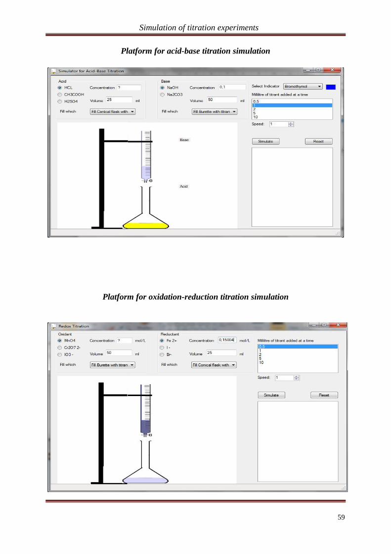
Simulation of titration experiments
59
Platform for acid-base titration simulation
Platform for oxidation-reduction titration simulation