multiple-wave lateral shearing interferometry for wave...

Multiple-wave lateral shearing interferometry forwave-front sensing

J.-C. Chanteloup

Multiple-wave achromatic interferometric techniques are used to measure, with high accuracy and hightransverse resolution, wave fronts of polychromatic light sources. The wave fronts to be measured arereplicated by a diffraction grating into several copies interfering together, leading to an interferencepattern. A CCD detector located in the vicinity of the grating records this interference pattern. Some ofthese wave-front sensors are able to resolve wave-front spatial frequencies 3 to 4 times higher than aconventional Shack–Hartmann technique using an equivalent CCD detector. Its dynamic is also muchhigher, 2 to 3 orders of magnitude. © 2005 Optical Society of America

OCIS codes: 120.5050, 120.3180, 120.2650, 050.1970, 070.4790, 070.2590, 070.5010, 100.5070,350.5030.

1. Introduction

Historically, the first wave-front sensor based on spa-tial phase sampling was probably the Scheiner disk,1in 1619. Since the invention of the laser, wave-frontmeasurement techniques are part of the necessarytools for laser beam characterization. The need of areference-free method explains why, until recently,the Hartmann test2,3 was the only widely used wave-front sensor for phase measurement, especially onlarge-aperture � � 10 cm� laser systems. Hartmann-Shack4 wave-front sensors were originally developedin the 1970s. They soon became the devices of choicefor astronomers looking for a wave-front sensor ableto collect 100% of the photons. They were lateradopted by laser physicists for their compactness andsimple alignment procedure.

The Laboratoire pour l’Utilisation des Lasers In-tenses (LULI), Ecole Polytechnique, France, pio-neered the use of achromatic multiple-wave lateralshearing interferometry (AMWLSI) for laser applica-tions in the late 1990s.5–9 The principle of this tech-nique relies on the generation of several replicas ofthe wave front to be evaluated using a grating. The

resulting interferogram is then recorded onto a CCDretina, and the acquired image is finally processedusing two-dimensional Fourier analysis to recoverthe phase with a high transverse and longitudinalresolution. For details regarding the principle of thetechnique, see the research of J. Primot.10,11 As anexample, an achromatic three-wave lateral shearinginterferometer12,13 (ATWLSI) relies on the use of atransmission grating creating three replicas of theinput wave front that are interfering together, result-ing in a honeycomblike interference pattern.

The ATWLSI has, for instance, been used to evalu-ate with a high precision the nonlinear index n2 offused silica8 and also to create an on-axis focal line.14

All the work performed at LULI, especially in adaptiveoptics, relied on the ATWLSI.5–7,9,15,16 This wave-frontsensor was also used extensively in this field at theCenter for Ultrafast Optical Sciences at the Universityof Michigan.17,18 This was also the case for phase-conjugation experiments at Troitsk Institute of Inno-vative and Thermonuclear Research in Russia.19

The ATWLSI appeared indeed to be a good candi-date for adaptive optics in lasers. For instance, in theframework of the European Union funded fifthProgramme-cadre Communautaire de Recherche etDéveloppement (Adaptool), it was cross evaluated bythe five leading European laboratories using intenselasers. The limited transverse resolution of the Shack–Hartmann (SH) technique was then highlighted.20

2. Achromatic Three-Wave Lateral ShearingInterferometer

The main components of an ATWLSI are described inthis section [grating (Subsection 2.A) and mask (Sub-

J.-C. Chanteloup ([email protected])is with Laboratoire pour l’Utilisation des Lasers Intenses, UnitéMixte de Recherche 7605, Centre National de la Recherche Scien-tifique, Comissariat a l’Energie Atomique, Ecole, Polytechnique-Universite Paris VI, Ecole Polytechnique, 91128 Palaiseau Cedex,France.

Received 2 April 2004; revised manuscript received 2 October2004; accepted 7 October 2004.

0003-6935/05/091559-13$15.00/0© 2005 Optical Society of America

20 March 2005 � Vol. 44, No. 9 � APPLIED OPTICS 1559

section 2.B)]. The fundamental operations of the re-covering algorithm are described, and the adjustablesensitivity leading to a high dynamic capability isexplained.

A. Achromatic Three-Wave Lateral ShearingInterferometer Grating

Looking in the far field, the perfect grating wouldsend exactly a third of the input energy in each sum-mit of an equilateral triangle: Tid��, ��. This field is aFourier plane, where transverse space coordinatesare ��, ��; coordinates in the real space are �x, y�.

Several algorithms can be used in order to optimizethe grating profile. Most of them start with a Fouriertransform of this energy distribution. The resultgives a very good approximation of the ideal trans-mittance tid�x, y� � A�x, y�exp�i��x, y�� of the grating.The grating used in the first generation of ATWLSI isa pure phase object. This constraint implies droppingthe amplitude term A�x, y� of the ideal transmittanceand replacing it with a constant term. We are apply-ing such a constraint in a Gerchberg–Saxton type ofalgorithm,21,22 which leads to the phase term ��x, y�plotted in Fig. 1.

The first generation of ATWLSI is based on anapproximated version of this phase distribution.A three-level-only phase plate. An ancestor of theATWLSI was the three-wave lateral shearing inter-ferometer.12 It was based on a splitting cube and amirror to generate the three replicas by reflectionson three different surfaces. But this device appearsto be difficult to use with a polychromatic lightsource (a femtosecond laser pulse, for instance). In-deed, the interfringe of the resulting interferogramwas then dependant upon the wavelength. In orderto make this three-wave lateral shearing inter-ferometer achromatic, it was then necessary to usea grating. This technique is used, for instance, inthe Mach–Zehnder grating.23

The grating we describe here is a pure phase object

working in transmission for a beam having a normalincidence. Its diffraction efficiency is optimum for aspecific wavelength �0. The elementary cell is a groupof three regular hexagons of respective height 0, �0�3,and 2�0�3, as shown in Fig. 2. This 2D diffractiveelement can also be seen as a superposition of threeone-dimensional (1D) gratings whose groove pitch isequal to

pas �3 hex

2 , (1)

where hex � 100 �m is the small dimension of ahexagon, as shown in Fig. 2.

Each of these three 1D gratings can be seen as“blazed” so that the energy of a wave at normal inci-dence would be almost entirely diffracted in ordersm � �1 with an angle � satisfying

pas[sin(0) � sin(�)] � m�. (2)

Using Eq. (1) leads to

sin(�) �2�

3 hex. (3)

Adding the fields of the three diffracted waves leadsto an intensity distribution (the honeycomblike inter-ferogram) from which the distance between two ad-jacent maxima can be extracted: the so-called“interfringe” (even if, in this case, fringes are dots):

if �2�

3 tan �. (4)

Fig. 1. Top view (upper-right insert) and lineout profile (thincurve) of the phase term of the Fourier transform of the idealenergy distribution needed in the far field. The bottom-left insert isa three-dimensional view of the real design of the grating, i.e.,hexagon-shaped mesas located either at an altitude of ��3 or 2��3above the silica substrate. The associated profile is represented bythe bold square line.

Fig. 2. Top view of the grating. White hexagons have an altitudeof 0, whereas respective altitudes of gray and black hexagons are�0�3 and 2�0�3. The distance pas is the pitch between grooves of aone-dimensional grating.

1560 APPLIED OPTICS � Vol. 44, No. 9 � 20 March 2005

Combining these last two equations, the interfringeexpression becomes

if � hex cos(�). (5)

The characteristic dimension (hex) of the grating istwo orders of magnitude larger than the wavelength.The angle � is consequently very small: dispersionproperties are indeed very weak. An expansionaround � is then acceptable:

if � hex�1 ��2

2 � . . . �. (6)

Even the zero-order approximation is valid since thenumerical calculation (� � 1.057 �m and hex� 100 �m) gives

if � hex(1 � 2.5 105 � . . . ). (7)

We can then consider

if � hex. (8)

Gray-level lithography is used to process thesegratings. The principle is described in Fig. 3. Avariable-transmittance mask is used (after develop-ment) in order to create a spatial modulation of thethickness of a photosensitive resin deposited onto asilica substrate. Choosing a resin having the correctindex of refraction may permit the process to bestopped after this step 1. The resulting plate mustthen be handled carefully because of the potentialfragility of the resin. For applications where morerobustness is required, one must pursue step 2: etch-ing of the substrate. Then, we obtain a robust silicaplate.

This overall process (using a pure phase gratingand approximating the phase profile with three levelsonly) explains why the actual grating exhibits theexperimental energy distribution shown in Fig. 4.Indeed, a nonnegligible amount of the input energy istransmitted by the grating in unwanted orders, cre-ating then several other perturbing replicas.

We are currently working on a new version of grat-

ings. Holography techniques should help obtain dif-fraction gratings having a much better efficiency.

B. Mask

Equation (8) shows that the interfringe is indepen-dent of �, justifying the achromatic qualification ofthe ATWLSI. Nevertheless, this wave-front sensor issomehow limited in spectral bandwidth, as is shownin this subsection.

In order to overcome the issue of unwanted diffrac-tion peaks, an order-selection plate has to be insertedin the common focal plane of the lenses of a telescopelocated between the grating and the sensor (Fig. 5).The widths of the holes are defined according to cri-teria linked to spectral overlap of high diffractionorders �m �1�. There are two consequences relatedto the use of this order-selection plate:

Fig. 3. Structuring the plate by lithography.

Fig. 4. Far-field distribution Texp��, �� of diffracted energy by thegrating used in the ATWLSI. Although most of the energy can befound in the three first orders, a nonnegligible amount of energy isstill diffracted elsewhere.

Fig. 5. Schematic view of a complete ATWLSI system. An order-selective plate (labeled zero-order beam stop) is inserted in themiddle of a telescope relaying the replication plane (i.e., the grat-ing) onto the CCD. Then only the three useful m � �1 orders areselected.


Y The overall system stays achromatic, but itsspectral bandwidth is limited (see Subsection 2.B.1).

Y Phase measurements become limited to wave-front distortions, leading to a focal energy transversedistribution smaller than the hole aperture (see Sub-section 2.B.2).

1. Spectral Bandwidth LimitationThe grating is working in the m � �1 order. It is

recommended to avoid overlap between higher orders�m � �1� of the spectral component �min of the lightsource and the m � �1 order of the spectral compo-nent �max. For a normal incidence at wavelength �,the “grating law” (2) gives

pas sin �m(�) � m�, (9)

where �m�� is the value of angle � linked to the orderm at wavelength �. Overlapping occurs when

[sin �m(�max) � sin �n(�min)] ) [m�max � n�min]. (10)

With m � �1 and n � �2, this equation is equivalentto

�max � 2�min. (11)

This equality defines ��ATWLSI � ��min, �max�, the spec-tral bandwidth of the ATWLSI. It is centered on �0,the wavelength for which the grating efficiency hasbeen optimized:

�0 ��min � �max

2 . (12)

The expression of the spectral bandwidth is then

��ATWLSI � [2�0�3, 4�0�3]. (13)

The mask’s holes are defining this bandwidth. In or-der to show this, let us first recall that � is the inci-dence of the three diffracted waves arriving at thefirst lens of the telescope (lens L1 of focal length f1).According to Eqs. (4) and (8), it satisfies

tan �(�) �2�

3 hex. (14)

Let r�� be the radial coordinate, in the focal plane ofL1, of a ray of wavelength � intercepting this lensunder incidence �:

r(�) � f1 tan �(�). (15)

Combining Eqs. (14) and (15),

r(�) �23

�

hex f1. (16)

In order to satisfy Eq. (13), the holes of the selective-order mask must then be limited by

rmin � r(�min) � 2r0�3,

rmax � r(�max) � 4r0�3, (17)

where r0 � r��0�.

2. Amplitude of Phase Distortions MeasurementLimitation

Let us now consider the spreading of the energydistribution in the focal plane for a given wavelength�. Ideally, whatever the wavelength:

Y The focal spot of the zero order should bemasked (condition c1).

Y The focal spot of the three first orders shouldnot be truncated (condition c2).

Condition c1 guarantees that only three orders areinterfering, whereas c2 means that the role of themask is to select the useful orders of diffraction andnot to act as a spatial filter, degrading the ability ofthe ATWLSI to detect highly distorted wave fronts.

The focal spots are identical for m � 0 and m ��1. For wavelength �0, c1 and c2 imply a doubleconstraint to the mean radius rfoc��0� of this focal spot:

rfoc(�0) � rmin, rfoc(�0) �rmax rmin

2 �rmin

2 . (18)

Let us assume that the three beams incident on lensL1 carry a flat phase and a constant amplitude profileover a circular pupil of diameter A. Their focal energydistribution is then called an Airy pattern.24,25 Itssize can be defined as the radius of the first dark ringof this distribution. At the central wavelength of thespectrum of the light source, its expression is

rAiry(�0) �1.22�0f1

2A. (19)

These beams are said to be limited by diffraction. Inother words, the transverse size of the focal energydistribution is limited by the diffraction of the waveon the edge of the A diameter pupil.

If, now, the incident beam is carrying optical aber-rations, its focal intensity distribution will spread.Let us call the limit of diffraction (LD) the ratio be-tween rfoc��, the mean radius of the aberrant focalspot, and rAiry��. A diffraction-limited beam is thencharacterized by an LD of unity, whereas LD isgreater than one for an aberrant beam. This criterion,although widely used in optics, gives almost no infor-mation regarding the nature of the carried phasedistortions, but it is a quick way to evaluate thetransverse quality of a light beam.

The largest focal spot measurable at �0 with theATWLSI can then be evaluated in terms of the limitof diffraction, LD0:


LD0 �rmin�2

rAiry(�0)�

49

A

1.22 hex. (20)

For a A � 1 cm diameter beam, this equation givesLD0 � 36 for the optimal wavelength �0 and hex� 100 �m. For the extreme wavelengths, �min and�max, the associated limits of diffraction LDmin andLDmax, are obviously equal to zero because the centerof their focal spot is located on the edge of the mask.It appears then pertinent to take into account thespectral bandwidth of the source �� 1, �2� in orderto evaluate the limit of diffraction for �1 and �2:

LD1 �r(�1) rmin

rAiry(�1)� LD0

(2�0 3��)(2�0 ��) , (21)

LD2 �rmax r(�2)

rAiry(�2)� LD0

(2�0 3��)(2�0 ��) . (22)

The above expressions are obtained while assumingthe source to be centered at the wavelength �0� ��1 � �2��2. As an example, laser pulses used atLULI26 satisfy �0 � 1.057 �m, �1 � 1.052 �m, �2� 1.062 �m, and then �� 1, �2� � 10 nm, whichleads to LD1 � 35.7 and LD2 � 35.3. The graph in Fig.6 shows the evolution of both branches (21) and (22)of the curve LD��LD0 in this specific case. Lookingat this curve, it appears that the total dynamic of theATWLSI is fully exploited only when the measure-ment is performed at the wavelength for which thedevice has been optimized. When the beam is verydistorted �LD0 � 36� or is small in diameter, thethree focal spots become large, and the mask starts toact as a spatial filter in a Fourier plane. The phaserecovered from the interference pattern recorded onthe CCD will then appear less aberrant than it reallyis. Figure 7 shows an ATWLSI with all its compo-nents.

C. Recovering Algorithm

A 2D Fourier analysis-based algorithm is used toextract the phase from the interference pattern re-corded by the CCD. Figure 8 describes its structure:

Step 1. A first Fourier transform is performed ontothe interferogram. The FT is a mathematical opera-tion known for keeping symmetry properties. It isthen not a surprise to observe a six-order symmetrypattern in the Fourier space: a zero-order harmonicsurrounded by six first-order harmonics. Owing tothe symmetry properties of the Fourier transform,only three of them carry different information.

Step 2. Any group of three first-order harmonicslocated on the vertices of an equilateral triangle isrelevant to recover the phase. These harmonics arethen windowed and extracted from the Fourier im-age.

Step 3. Each of the three small images resultingfrom the previous spectral windowing operation isthen processed through an inverse Fourier transformoperation. The three derivatives of the phase we are

looking for are extracted from the resulting compleximage.

Step 4. Finally, the three derivatives are integratedto recover the final phase.

In practice, several other image-processing opera-tions (such as thresholding, masking, least-squareprojection, or Fourier integration) are required.12,13

The central harmonic can also be used in order torecover the amplitude transverse profile of the ana-lyzed beam (Fig. 9). The overall process is here morestraightforward.

Fig. 6. Shape of LD��LD0 in the case where the central wave-length is equal to 1 �m.

Fig. 7. Picture of an ATWLSI. Scale is given by the 25 mm pitchof the breadboard holes.

Fig. 8. Description of the phase-recovering algorithm used foranalysis of ATWLSI interferograms.


The ATWLSI allows the recovery of three deriva-tives of the phase in three directions�U0°, U�120°, U120°� pointing at 120° from each other.It leads to interesting properties specific to ATWLSI:

First, the integration of three such derivativesgives a more accurate reconstruction of the phasethan two derivatives at 90° from each other (as in aShack–Hartmann, or for the achromatic quadri-wavelateral shearing interferometer (AQWLSI) describedin Section 3) or only one derivative (as with a shear-plate or a Mach–Zehnder interferometer).

Also, it can be demonstrated12,13 that the sum ofthe three derivatives obtained should mathemati-cally cancel if the overall wave-front sensor (grating,CDD, . . .) were perfect:

S(r) � � �(r) · (U0° � U120° � U120°) � 0, (23)

where r is the transverse coordinate and ��r� is thephase we are looking to recover.

In practice, this sum is slightly different from zeroowing to imperfections of the wave-front sensor itself.It can be shown12 that the mean value of S�r� over thepupil is directly linked to the phase root-meansquare, �:

�S(r)2 � 3�2. (24)

The ATWLSI possesses then the unique property ofgiving the phase profile together with an evaluationof the accuracy of this measurement.

D. Adjustable Sensitivity of the Achromatic Three-WaveLateral Shearing Interferometer

A large dynamic range characterizes wave-front sen-sors of the AMWLSI family. Such interferometers areindeed able to detect phase distortions of several tensof waves but also of very small fractions of a wave��100�. These sensors indeed have an adjustablesensitivity.

Let us call x and y the transverse coordinates of alight beam from which the phase ��x, y� needs to berecovered. Oz is the direction of propagation. By us-ing the diffractive grating described above, it is pos-sible to duplicate � in such a way that both replicas�1, R and �2, R are tilted with respect to each other byan angle �. These replicas are shown in Fig. 10 in theplane xOz.

Their mean wave vectors k1 and k2 are not col-linear but belong to xOz. The tilt of �1, R and �2, R is

performed around the axis Oy, and we have

�1, R(x, y) � �(x, y) ��a�

x,

�2, R(x, y) � �(x, y) �a�

x, (25)

where a � tan��2��2. The plane where � is dupli-cated is called the replication plane PR. This plane(the grating for the ATWLSI), when imaged onto asensor, allows the recording of the interferogram IR:

IR(x, y) � 2I0(x, y){1 � cos[�1, R(x, y) �2, R(x, y)]}.(26)

Combining Eqs. (25) and (26), we have

IR(x, y) � 2I0(x, y)1 � cos�2�

�ax��. (27)

This equation shows that, whatever the distortions of��x, y� are, IR exhibits a regular fringe distributioncharacterized by an interfringe i � ��a. Such an ob-servation plane is called the “zero-sensitivity plane”of the interferometer, where all the information re-garding ��x, y� is lost.

After duplication, �1 and �2 will shear from each

Fig. 9. Spectral windowing operation for recovering the ampli-tude.

Fig. 10. Upper figure shows (in the plane xOz) both replicas �1

and �2 (thin curves) of the phase � in their replication plane PR

� xOy (i.e., the grating plane). After being replicated, they prop-agate along the direction of the mean wave vectors k1 and k2 (boldcurves). While doing so, they transversally shear from each other.The middle part of this figure shows a schematic view of theinterference pattern IR�x, y� obtained in PR, a regular alignment ofdark and bright fringes; information about the phase is lost. In aplane of observation PZ parallel to PR, the interference patternIZ�x, y� (lower part of the figure) shows then distortions linked tothe derivative of ��x, y� along x.


other while propagating since they follow the direc-tions of their respective wave vectors k1 and k2 (Fig.10). If now, the observation is performed in a plane PZ

located after PR at a distance z, the transverse shearbetween both replicas becomes

dx �az2 , (28)

and the recorded interferogram IZ satisfies

IZ(x, y) � 2I0(x, y){1 � cos[�1, z(x, y) �2, z(x, y)]},(29)

with, this time,

�1, z(x, y) � ��x �dx2 , y��

�a� �x �

dx2 �,

�2, z(x, y) � ��x dx2 , y�

�a� �x

dx2 �. (30)

Only the modulation M�x, y� of the intensity distri-bution IZ�x, y� carries useful information:

M(x, y) � cos[�1, z(x, y) �2, z(x, y)]. (31)

Combining this equation with Eq. (30), one obtains

M(x, y) � cos2�

�ax � ��x �

dx2 , y� ��x

dx2 , y��.

(32)

Taking into account the dependence of dx with z givenby Eq. (28), we obtain

M(x, y) � cos2�

�ax � ��x �

a4 z, y�

��x a4 z, y��. (33)

By introducing the interfringe, i � ��a, and by look-ing only at the x dimension perpendicular to thefringe, we have

M(x) � cos2�xi � �(x � �z�4i) �(x �z�4i)�. (34)

The first term �2�x�i� of the cosine argument definesthe carrier modulation of the information containedin the second term, ��x, z� � ��x � �z�4i� ��x �z�4i�. If the transverse shear, dx � �z�2i, is suf-ficiently weak that the phase variation, ��x, z�, canbe considered as linear, it appears then that IZ�x, y�allows recovering of the partial derivative in x. Let uscall �x��xi, z� the partial derivative at point xi:

�x�(xi, z) ��(xi � �z�4i) �(xi �z�4i)

�z�2i for z � 0.

(35)

Let us evaluate the bandwidth associated to the mea-surement of �x��xi, z�. Whatever the values of x and zare, one must have ��xi, z� � 2� in order to avoidany ambiguity in fringe attribution. Indeed, if��xi, z� � 2�, Eq. (34) then simplifies locally intoM�xi� � cos�2�xi�i�; in other words, the carrier fre-quency is not suitable anymore. It becomes then forthe maximum acceptable local tilt:

�max�(xi, z) � 4�

�

iz. (36)

Let us assume that �� allows an optimal mea-surement (the fringe is shifting by half a period owingto the local gradient). It appears then that, in a pointwhere this condition is satisfied, the optimally detect-able local derivative �x��xi, z� � i2��z is varyinginversely with z. This means that, when the plane ofobservation PZ is very far from PR, it is possible todetect a very weak local gradient with an optimalquality. Conversely, when PZ is getting closer (smallz), it becomes then possible to detect very large gra-dients. In summary, this interferometer is character-ized by a large dynamic of measurement owing to asensitivity adjustable with z according to the ampli-tude of the wave-front distortions to be detected.

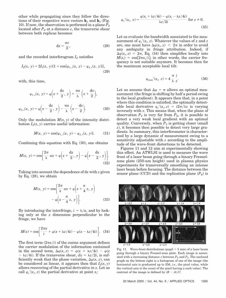
Figures 11 and 12 aim at experimentally showingthis effect. An ATWLSI is used to measure the wavefront of a laser beam going through a binary Fresnel-zone plate (250-nm height) used in plasma physicsexperiments for transversally smoothing an intenselaser beam before focusing. The distance between thesensor plane (CCD) and the replication plane �PR� is

Fig. 11. Wave-front distributions �pupil � 5 mm� of a laser beamgoing through a binary Fresnel-zone plate. Each image is associ-ated with a increasing distance z between PR and PZ. The enclosedgraph on the bottom right is a histogram of one of the image (thehorizontal axis is graduated up to 256, i.e., the pixel value, whilethe vertical axis is the count of the pixel having a such value). Thecontrast of the image is defined by �B A��C.


adjusted from z�hex � 5 to z�hex � 60. Figure 11shows a succession of 13 wave-front images obtainedwith the ATWLSI for these different values of z�hex.hex is the characteristic dimension of the grating [seeEqs. (1) and (4)].

It is useful to compute the contrast of these wave-front images:

contrast �(B A)

C . (37)

The wave front under study is generated by a two-level-only phase plate, making such a quantity rele-vant here. C is the sensor dynamic; 256 gray levels inthis case. The bottom right of Fig. 11 shows how, fromthe histogram of each of the 13 wave-front images, weextract the difference �B A� between the two peaksassociated with each of the two levels of the phase.The use of a perfect binary Fresnel-zone plate com-bined with an ideal sensor would give B A � C,leading to a contrast of unity.

By plotting the contrast versus z (Fig. 12), it ap-pears that it increases with z. It should be noted thatthe transverse resolution is simultaneously decreas-ing with z (less-fine defects are observed for highvalues of z).

This means that, for this specific 250 nm-heightphase distortion, it is required to record the interfero-gram at a distance of 4 to 6 mm from the replicationplane in order to have the best sensitivity (best con-trast on the phase image). Above 6 mm, adjacentfringes start collapsing, making the interferogramanalysis impossible.

3. Achromatic Quadri-Wave Lateral ShearingInterferometer

Primot et al.27 gave a demonstration of this deviceunder the name of modified Hartmann mask. Theterminology used here is voluntarily linked to thepreviously described ATWLSI. It is a semantic choicesimply from the fact that the AQWLSI belongs to thecommon AMWLSI family. This interferometer relies

on the use of four replicas, when three were requiredin the ATWLSI.

The exploration of this alternative solution is mo-tivated by the lack of compactness of the ATWLSI. Itis indeed shown in the previous section that, inorder to obtain a distribution of the energy of theincident beam in only the three useful orders, animaging and order-selection device must be added,making the ATWLSI more difficult to align and lesscompact. The AQWLSI is explored in order to over-come this issue.

A. Achromatic Quadri-Wave Lateral ShearingInterferometer Grating

We follow a procedure identical to the one describedin Section 2: We observe energy distributions intothe far-field plane, assumed here to be equivalent toa Fourier-space plane; ideally all the energy dif-fracted by the perfect grating should be located atthe four vertices of a square [Eq. (38), where thetilde sign (˜) symbolizes the Fourier transform]. Thechoice of a square in place of any other quadrilateralfigure is mainly driven by symmetry reasons; for sim-ilar reasons, an equilateral triangle was chosen forthe ATWLSI instead of an arbitrary triangle:

t̃id(�, �) � ��v 1a0

, � 1a0��

1a0

, � �1a0�

� �� 1a0

, � 1a0��

1a0

, � �1a0�,(38)

�� x, � � ��y� are the Fourier-conjugated coor-dinates of �x, y� in the real space, where � is thewavelength. Going back to the real space through aninverse Fourier transform leads to the following sim-ple expression for the ideal transmittance of the grat-ing:

tid(x, y) �12�cos 2�(x � y)

a0�� cos2�(x y)

a0� . (39)

Let the ideal transmittance be reformulated as fol-lows:

tid(x, y) � sign[tid(x, y)]abs[tid(x, y)], (40)

where the sign and abs functions are, respectively,the sign and the absolute value of the transmittance.Experimentally obtaining the sign function is rela-tively simple. Indeed, the tsign�x, y� � sign�tid�x, y��distribution can be obtained with a phase chessboardhaving two altitudes of 0 and �. Indeed exp�i�� 1, whereas exp�i0� � 1 (with i2 � 1). The chess-board period needs to be equal to p � a0��2. A purephase plate (made of fused silica, for instance) mod-ulated according these rules is not difficult to process.However, this is not the case for the tabs�x, y�� abs�tid�x, y�� distribution. Creating a plate with a

Fig. 12. Contrast evolution between PR�z�hex � 0� andPZ�z�hex � 60�. z�hex is the distance to the replication gratingnormalized to grating characteristic dimension hex � 100 �m.


transmission varying according to the semisinusoidalarches of this distribution is more difficult, especiallyif the process used to do so must avoid the creation ofany unwanted phase modulation: we are here indeedlooking for a pure amplitude modulation for tabs�x, y�.

As for the ATWLSI, approximating the ideal trans-mittance also appears to be required. The idea is togenerate tabs�x, y� with only a two-level amplitude dis-tribution. Figure 13 describes this operation. The re-sulting amplitude part of the grating appears to be asimple Hartmann plate with holes of square aperturea distributed over a Cartesian grid of period p. Equa-tion (41) gives the expression of such an approxi-mated version of tabs�x, y�:

tabsapprox(x, y) � �a, a(x, y) � �a0��2 (x) � �a0��2 (y),

(41)

where �p�x� is the “comb” function, i.e., a successionof Dirac ��x� functions regularly spaced with a p pe-riod, and �a, a�x, y� is a “gate” function having thesame transverse aperture a in both directions.

We show that by choosing carefully the ratio a�p, itis possible to select in which order we want the en-ergy to be diffracted. In order to make it easier tovisualize graphically, (Fig. 14) the individual contrib-uting effect of tsign�x, y� and tabs�x, y�, let us continuethe demonstration with a 1D approach. We have then

tabsapprox(x) � �a(x) � �p(x) (42)

and for its Fourier transform

t̃absapprox(�) �

sin(��a)��a � �1�p(�). (43)

The grating is made of the combination of the Hart-

mann plate and the phase chessboard having thesame period p. We have then the following 1D expres-sion for the transmittance of our complete gratingand its Fourier transform:

tapprox(x) � �a(x) � [�p(x)exp(i�x�p)] (44)

t̃approx(�) �sin(��a)

��a �1�p(�) � �� 1

2p��. (45)

Comparing Eqs. (43) and (45) reveals that the effectof the phase chessboard is simply to translate by 1�2pthe Dirac comb of period 1�p. As a consequence, thereis no more energy observed in the zero order (arrownumber 3 in Fig. 14). This is already a major improve-ment from the grating used for the ATWLSI. But it isstill possible to do better.

Indeed, by adjusting the respective values of theHartmann plate aperture a and the period p, we cansuppress several other unwanted diffraction orders.The idea is to make the orders that are to be canceledcoincide with the zeros of the sin��a��a� function.Figure 14 describes this effect. A simple geometricalargument shows that the following condition satisfiesthe cancellation of orders labeled 1 and 4:

a � 2p�3. (46)

Let us now visualize the effect of Eq. (46) in a 2Dspace. Figure 15 details what can be observed in theFourier plane, whereas Fig. 16 gives a picture of thereal plane, i.e., the plane where the CCD sensor islocated. Experimentally, we observe, in the Fourierplane, the distribution shown in Fig. 17. Such a dif-

Fig. 13. Top-right sketch is the phase part of the AQWLSI grat-ing, i.e., a phase chessboard equivalent to sign�tid�x, y��. The top-left sketch is the amplitude part, i.e., an approximation ofabs�tid�x, y��. This part appears to be a simple Hartmann plate withholes of square aperture a distributed over a Cartesian grid ofperiod p. The bottom curves show the lineout of abs�tid�x, y�� (se-misinusoid arches curve) and its approximation (rectangularcurve).

Fig. 14. Energy distribution t̃absapprox�� given by a Hartmann

plate of aperture a and period p is shown in this graph: The energyis located at the summit of each bold arrow (five of them arerepresented here with numbers in square boxes). The energy dis-tribution t̃ approx�� given by the same Hartmann plate combinedwith a phase chessboard of period p is also shown: The effect of thephase chessboard is to translate the previous set of arrows (i.e.,energy) by 1�2p to give the dashed arrows (the new positions arelabeled ① to ⑤ ). Arrows ① and ④ are replaced by two stars at theplace where they should be located. There is in fact no energy atthese positions owing to the presence of the zeros � � 1�a� of thesin��a��a� envelope. In order to achieve the cancellation of thistwo orders, the condition a � 2p�3 must be satisfied.


fraction pattern allows using the grating simply asthe microlens array of a SH wave-front sensor: in-deed, it just needs to be located in front of a CCDwithout the need for any extra image relay optics.The overall AQWLSI interferometer is much morecompact than the ATWLSI. The angle ��2 underwhich the four orders are being diffracted satisfies

�2p sin��

2�� . (47)

The grating used to produce the interferogram ofFig. 16 is characterized by a � 26 �m and p

� 39 �m. It consequently gives a value of 36.26 mradfor � at 1 �m. This angle is very small; this grating(like the ATWLSI’s one) is then not a very strongdispersing element.

B. Transverse Resolution of the Achromatic Quadri-WaveLateral Shearing Interferometer

Figure 18 gives experimental measurements of a dis-torted wave front recorded with an AQWLSI. Thecomparative analysis of the transverse resolution isgood but does not appear very satisfying with respectto what was achieved with the ATWLSI. A reason isthe fact that the AQWLSI allows recovery of only twoderivatives, whereas the ATWLSI gives one more.The reconstruction accuracy is therefore degraded. Itis also important to take into account the distance zbetween the replication plane and the sensor. In thecase of the ATWLSI, the grating plane is imaged onto

Fig. 15. Looking in the far field (for instance, in the focal plane ofa lens located after the grating), we have access to the energydistribution in different orders of diffraction. In the left and rightimages, we see that there is no energy in the zero order (thanks tothe phase chessboard). Let us call the four first orders the fourpeaks located the closest to the center of the field of this spectrum(all four belong to the same ring centered in the center of the field;ring one is in the middle image). In the left image, we can see eightpeaks located in a second ring surrounding these four peaks (a ��2p�3). These orders of diffraction vanish in the right picture �a� 2p�3�.

Fig. 16. Insert shows an AQWLSI grating, a Hartmann maskmodified by the adjunction of a phase chessboard; this is why thiswave-front sensor is also called modified Hartmann mask.32 Themain picture is an interference pattern obtained with an AQWLSIbased on a grating characterized by a � 26 �m and p � 39 �m.

Fig. 17. Energy distribution recorded in the focal plane of a lenslocated right after the grating. More than 87% of the incidentenergy is distributed in the four first orders. Less than a percent ispresent in the zero order, while no energy can be recorded in ring2. The remaining energy distributed over a large number of higherorders does not affect the measure.

Fig. 18. Interferograms and (inserts) recovered laser phase ob-tained with an AQWLSI. The laser wave front was modulatedusing a liquid-crystal optical valve.5 The pupil is �5 mm and dis-tortions amplitude is �1 wave.


the CCD with a relay telescope, creating a virtualreplication plane. It is consequently possible to adjustcontinuously the distance z from 0 to several centi-meters. On the other hand, for the AQWLSI, thereplication plane is real and equivalent to the gratingplane; consequently, mechanical constraints do notpermit getting too close to the sensor �z � 0�.

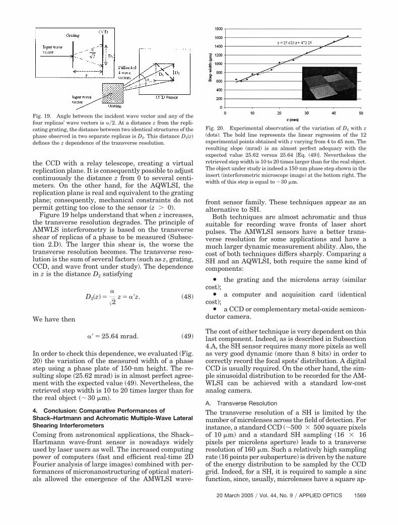
Figure 19 helps understand that when z increases,the transverse resolution degrades. The principle ofAMWLS interferometry is based on the transverseshear of replicas of a phase to be measured (Subsec-tion 2.D). The larger this shear is, the worse thetransverse resolution becomes. The transverse reso-lution is the sum of several factors (such as z, grating,CCD, and wave front under study). The dependencein z is the distance D2 satisfying

D2(z) ��

�2z � ��z. (48)

We have then

�� 25.64 mrad. (49)

In order to check this dependence, we evaluated (Fig.20) the variation of the measured width of a phasestep using a phase plate of 150 nm height. The re-sulting slope �25.62 mrad� is in almost perfect agree-ment with the expected value (49). Nevertheless, theretrieved step width is 10 to 20 times larger than forthe real object ��30 �m�.

4. Conclusion: Comparative Performances ofShack–Hartmann and Achromatic Multiple-Wave LateralShearing Interferometers

Coming from astronomical applications, the Shack–Hartmann wave-front sensor is nowadays widelyused by laser users as well. The increased computingpower of computers (fast and efficient real-time 2DFourier analysis of large images) combined with per-formances of micronanostructuring of optical materi-als allowed the emergence of the AMWLSI wave-

front sensor family. These techniques appear as analternative to SH.

Both techniques are almost achromatic and thussuitable for recording wave fronts of laser shortpulses. The AMWLSI sensors have a better trans-verse resolution for some applications and have amuch larger dynamic measurement ability. Also, thecost of both techniques differs sharply. Comparing aSH and an AQWLSI, both require the same kind ofcomponents:

Y the grating and the microlens array (similarcost);

Y a computer and acquisition card (identicalcost);

Y a CCD or complementary metal-oxide semicon-ductor camera.

The cost of either technique is very dependent on thislast component. Indeed, as is described in Subsection4.A, the SH sensor requires many more pixels as wellas very good dynamic (more than 8 bits) in order tocorrectly record the focal spots’ distribution. A digitalCCD is usually required. On the other hand, the sim-ple sinusoidal distribution to be recorded for the AM-WLSI can be achieved with a standard low-costanalog camera.

A. Transverse Resolution

The transverse resolution of a SH is limited by thenumber of microlenses across the field of detection. Forinstance, a standard CCD (�500 � 500 square pixelsof 10 �m) and a standard SH sampling (16 � 16pixels per microlens aperture) leads to a transverseresolution of 160 �m. Such a relatively high samplingrate (16 points per subaperture) is driven by the natureof the energy distribution to be sampled by the CCDgrid. Indeed, for a SH, it is required to sample a sincfunction, since, usually, microlenses have a square ap-

Fig. 19. Angle between the incident wave vector and any of thefour replicas’ wave vectors is ��2. At a distance z from the repli-cating grating, the distance between two identical structures of thephase observed in two separate replicas is D2. This distance D2�z�defines the z dependence of the transverse resolution.

Fig. 20. Experimental observation of the variation of D2 with z(dots). The bold line represents the linear regression of the 12experimental points obtained with z varying from 4 to 45 mm. Theresulting slope (mrad) is an almost perfect adequacy with theexpected value 25.62 versus 25.64 [Eq. (49)]. Nevertheless theretrieved step width is 10 to 20 times larger than for the real object.The object under study is indeed a 150 nm phase step shown in theinsert (interferometric microscope image) at the bottom right. Thewidth of this step is equal to �30 �m.


erture (the CCD plane being in the vicinity of the focalplane of the microlenses). The recovery of the localgradient is usually performed through an evaluation ofthe centroid position of this focal-plane energy distri-bution. The better this evaluation is, the more accu-rately the wave front is being reconstructed, andgetting an accurate value for the centroid of each focalspot requires such a high sampling rate.

In the case of the AMWLSI, the energy distributionto be sampled is an interferogram having a sinusoidalmodulation. Efficiently sampling a sinusoid requiresa very limited number of points. Indeed, it requiresfewer CDD pixels to sample a single-spatial-frequency signal such as a sine function rather thana sinc function carrying multiple spatial frequencies.For both ATWLSI and AQWLSI, the sampling rate isbetween three and four CCD pixels per fringe. Intheory, the transverse resolution of AMWLSI is closeto the distance between fringes, i.e., 30 to 40 �m forthe same standard CCD. AMWLSI wave-front sen-sors thus have the potential of being almost fourtimes better at resolving than SH sensors. Experi-mentally, this has been verified for AMWLSI forslow-varying wave-front distortions (fifth-order geo-metrical aberrations, for instance). As soon as thewave front to be measured starts exhibiting largegradients (such as those shown in Fig. 8 and insert ofFig. 20), the behavior of ATWLSI and AQWLSI dif-fers significantly: ATWLSI remains very accurate,whereas AQWLSI shows very strong degradation intransverse accuracy as for a SH. Figure 20 showsindeed that the retrieved step width is 10 to 20 timeslarger than for the real object. This undermines se-riously the capacity of AQWLSI to resolve fast-varying transverse structures. The three-derivatives-based ATWLSI sensor appears consequently verymuch more suited for accurately measuring suchwave-front distortions than its two-derivatives-basedcounterpart, namely, SH and AQWLSI.

B. Dynamic Range

In order to evaluate the maximum gradient measure-ment dynamic range for both techniques, we look at a

local level, i.e., across a microlens of aperture A� andfocal length f for a SH and across a fringe of width iand at a distance z for the AMWLSI. The maximumlocal gradient detectable with a SH is

�max�(xi, f) �2�

�

A��2f . (50)

Indeed, a wave carrying a local gradient above thisvalue would not be correctly evaluated since the en-ergy focused by this specific microlens would not onlybe illuminating its own subaperture of pixels �16� 16� but also the neighboring one.

For an AMWLSI, the maximum local gradient de-tectable exhibits a very similar expression (z, beingthe distance between the detector and the grating):

�max�(xi, z) � 4�

�

iz. (51)

In fact, if we use (as was suggested in the previoussubsection) A� � 160 �m and i � 40 �m, we see thatf and z have exactly the same role. For a short focallength f (for SH) or a short distance z between detec-tor and grating (for AMWLSI), the strongest gradi-ents can be detected. A standard value for f is�10 mm. For an AMWLSI, it is possible to make zvarying between 0.1 and 100 mm, allowing then thiswave-front sensor to provide a dynamic range 3 or-ders of magnitude higher than that of a Shack–Hartmann wave-front sensor. Table 1 summarizesthe respective performances of these wave-front sen-sors.

The author thanks Jérome Primot, ClémenceDaëron, and Mathieu Cohen for fruitful discussionand collaboration on this work.

References1. C. Scheiner, Sive fundamentum opticum (Oculus, Innsbruck,

Germany, 1619).2. J. Hartmann, “Objektivuntersuchungen,” Z. Instrumentenkd

24, 1–21 (1904).

Table 1. Respectives Performances of SH, ATWLSI, and AQWLSI Wave-Front Sensors

Properties Shack–Hartmann ATWLSI AQWLSI

Number of derivatives recovered 2 3 2Medium: �16 pixels Very good: � 4 pixels Good: � 4 pixels

Transverse resolution(slow-varying phase)

(Limited by microlensaperture)

�z � 0� (z limited by hardware:z � 0)

Transverse resolution(fast-varying phase)

Poor Very good (small z) Relatively poor (z limited byhardware)

Compactness/alignment Good ��10 cm� Poor (30 to 50 cm) (imagerelay required)

Good ��10 cm�

Dynamic Poor (fixed by microlensfocal length)

Very good (adjustable fromz � 0)

Good (adjustability limited byhardware: z � 0)

Error estimation Poor Good (3 derivatives) Poora

aAQWLSI manufacturers like Phasics are currently working on improving error-estimation evaluation. Providing such evaluation to theuser would be a clear advantage over a SH (besides dynamic and cost).


3. S. Hawkes, J. Collier, C. Hooker, C. Reason, C. Edwards, C.Hernandez-Gomez, C. Danson, and I. Ross, “Adaptive opticstrials on Vulcan,” Central Laser Facility Annual Rep.2000/2001 (Rutherford Appleton Laboratory, Didcot, UK,2001), p. 153.

4. R. V. Shack and B. C. Platt, “Production and use of a lenticularHartmann screen,” J. Opt. Soc. Am. 61, 656–660 (1971).

5. J.-C. Chanteloup, B. Loiseaux, J.-P. Huignard, G. Mourou, andH. Baldis, “Wave-front detection and correction for ultra-intense laser systems,” Solid State Lasers for Application toInertial Confinement Fusion, M. L. André, ed., Proc. SPIE3047, 227–338 (1997).

6. J.-C. Chanteloup, B. Loiseaux, J.-P. Huignard, and A. Migus,“Liquid crystal based adaptive optics setup for laser wave frontcorrection,” in Laser Technology for Laser Guide Star AdaptiveOptics Astronomy, N. Hubin, ed., ESO Proc. 55, 23–26 (1997).

7. J.-C. Chanteloup, H. Baldis, A. Migus, G. Mourou, B. Loiseaux,and J.-P. Huignard, “Nearly diffraction-limited laser focal spotobtained by use of an optically addressed light valve in anadaptive-optics loop,” Opt. Lett. 23, 475–477 (1998).

8. J.-C. Chanteloup, F. Druon, M. Nantel, A. Maksimchuk, and G.Mourou, “Single-shot wave-front measurements of high-intensity ultrashort laser pulses with a three-wave interferom-eter,” Opt. Lett. 23, 621–623 (1998).

9. B. Wattellier, J.-C. Chanteloup, J. P. Zou, C. Sauteret, and A.Migus, “Adaptive optics technique for wave front correction ofmulti-terawatt Nd:glass laser chain,” presented at the Confer-ence on Lasers and Electro-Optics, Baltimore, Md., 23–28 May1999.

10. J. Primot, “Three wave lateral shearing interferometer,” Appl.Opt. 32, 6242–6249 (1993).

11. J. Primot and L. Sogno, “Achromatic three-wave (or more)lateral shearing interferometer,” J. Opt. Soc. Am. A 12, 2679–2685 (1995).

12. L. Sogno, “L’interféromètre à décalage Tri-latéral: une nou-velle technique d’analyse de surface d’onde,” Ph.D. thesis (Uni-versité Paris XI, Orsay, France, 1996).

13. J.-C. Chanteloup, “Contrôle et mise en forme des fronts dephase et d’énergie d’impulsions lasers brèves ultra-intenses,”Ph.D. thesis (Ecole Polytechnique, Palaiseau, France, 1998).

14. B. Wattellier, C. Sauteret, J.-C. Chanteloup, and A. Migus,“Beam-focus shaping by use of programmable phase-only fil-ters: application to an ultralong focal line,” Opt. Lett. 27, 213–215 (2002).

15. J. Fuchs, B. Wattellier, H. Bandulet, P. Michel, J. P. Zou, J.-C.Chanteloup, C. Labaune, A. Michard, S. Depierreux, A. Kudr-

yashov, and A. Aleksandrov, “Wave front correction fordiffraction-limited focal spot on 80 J�1 ns laser facility,” pre-sented at International Quantum Electronics Conference/Conference on Lasers, Applications, and Technologies, Mos-cow, Russia, 27–28 June 2002.

16. B. Wattellier, J. Fuchs, J.-P. Zou, J.-C. Chanteloup, H. Ban-dulet, P. Michel, and C. Labaune, “Generation of a single hotspot by use of a deformable mirror and study of its propagationin an underdense plasma,” J. Opt. Soc. Am. B 20, 1632–1642(2003).

17. F. Druon, G. Chériaux, J. Faure, J. Nees, M. Nantel, A. Mak-simchuk, G. Mourou, J.-C. Chanteloup, and G. Vdovin, “Wavefront correction of femtosecond terawatt lasers using deform-able mirrors,” Opt. Lett. 23, 1043–1045 (1998).

18. F. Druon, M. Nantel, G. Vdovin, A. Maksimchuk, J.-C. Chan-teloup, J. Nees, and G. Mourou, “Single-shot B-integral wave-front correction of femtosecond laser pulses,” in Conference onLasers and Electro-Optics, Vol. 6 of 1998 OSA Technical DigestSeries (Optical Society of America, Washington, D.C., 1998),pp. 279–280.

19. V. I. Sokolov, M. I. Pergament, A. M. Nugumanov, and R. V.Smirnov, “Phase measurements under three wave mixing in anonlinear crystal,” Opt. Commun. 183, 515–522 (2000).

20. B. Le Garrec, “Adaptive optics operation for lasers: secondmeeting report,” contract HPRI-CT-1999-50012 (Commissar-iat à l’Energie Atomique, Paris, 2000).

21. R. W. Gerchberg and W. O. Saxton, “A practical algorithm forthe determination of phase from image and diffraction planepictures,” Optik (Stuttgart) 35, 237–246 (1972).

22. Y. M. Bruck and L. G. Sodin, “On the ambiguity of the imagereconstruction problem,” Opt. Commun. 30, 304–307 (1979).

23. G. J. Swanson, “Broad-source fringes in grating and conven-tional interferometers,” J. Opt. Soc. Am. A 1, 1147–1153(1984).

24. G. B. Airy, “On the diffraction of an object-glass with circularaperture,” Trans. Cambridge Philos. Soc. 5, 283–291 (1835).

25. M. Born and E. Wolf, Principles of Optics, 6th ed. (Pergamon,Oxford, UK, 1989), pp. 395–398.

26. J. P. Zou and C. Sauteret, “The LULI 100-TW Ti:sapphire/Nd:Glass laser: a first step towards a high performance petawattfacility,” Solid State Lasers for Application to Inertial Confine-ment Fusion, W. H. Lowdermilk, ed., Proc. SPIE 3492, 94–97(1998).

27. J. Primot and N. Guerineau, “Extended Hartmann test basedon the pseudoguiding property of a Hartmann mask completedby a phase chessboard,” Appl. Opt. 39, 5715–5720 (2000).


multiple-wave lateral shearing interferometry for wave...

Documents