nonclassical interferometry - geo600schnabel/vorl_ss06.pdf · nonclassical interferometry i....
TRANSCRIPT
Nonclassical InterferometrySlide presentation accompanying the
Lecture by Roman SchnabelSummer Semester 2006
Universität HannoverInstitut für Gravitationsphysik,
Max-Planck Institut für Gravitationsphysik (Albert Einstein Institut)
Callinstr. 38, D-30167 Hannover
[email protected]/personal/schnabel.html
Nonclassical InterferometryI. Introduction
1. Gravitational Wave Detection2. Classical Interferometry
II. Interferometer Quantum Noise: Basics and Tools3. Quantum Noise in Laser Interferometry4. Quantum Noise Spectral Densities5. Interferometer Readout: Homodyne versus Heterodyne Detection6. Quantum Noise of Sideband Modulation Fields7. Quadrature Input-Output Relations
III. Schemes for Nonclassical (Quantum-Non-Demolition) Interferometers8. Simple Michelson Interferometer with Squeezed Light Input9. “Variational Output” (Frequency dependent homodyne detection)
10. The Optical Spring Interferometer11. A Squeezed Light Upgraded GEO600 Detector? 12. The Speed Meter Idea and Sagnac Interferometer13. Optical Bars
3
I. Introduction 1. Gravitational Wave Detection
TopicsWhat are gravitational waves?Detectors on ground: GEO600, LIGO, VIRGO, TAMADetectors in space: LISAInterferometer quantum noise
Literature• P. Aufmuth and K. Danzmann, Gravitational wave detectors,
New Journal of Physics 7, 202 (2005), http://www.njp.org
• N. Robertson, Laser interferometric gravitational wave detectors, Classical and Quantum Gravity 17, R19 (2000).
4
Gravitational Waves
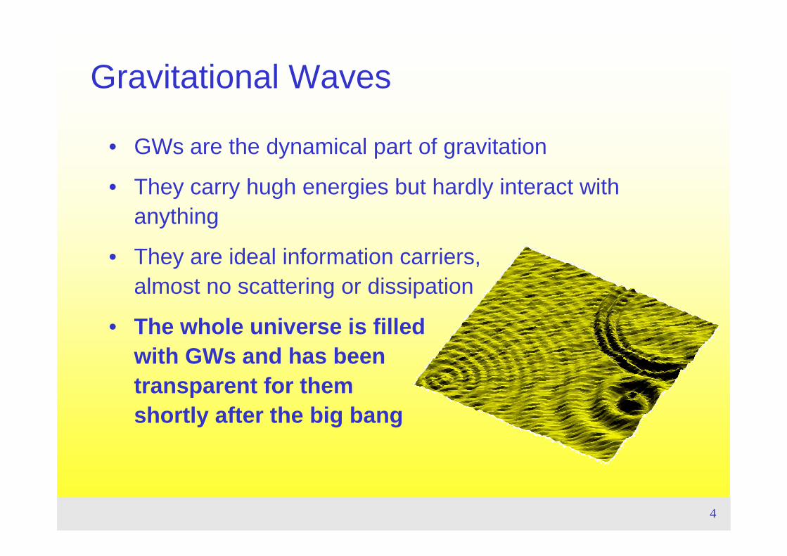
• GWs are the dynamical part of gravitation
• They carry hugh energies but hardly interact with anything
• They are ideal information carriers, almost no scattering or dissipation
• The whole universe is filled with GWs and has been transparent for them shortly after the big bang
5
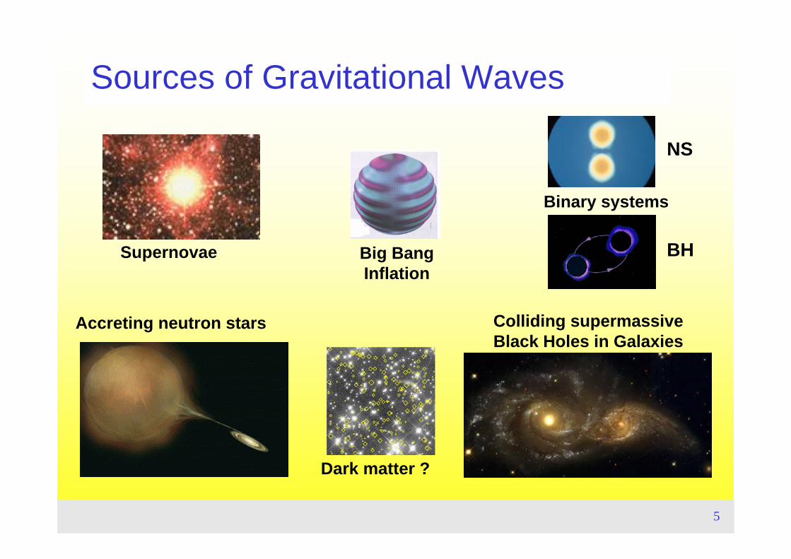
Sources of Gravitational Waves
Supernovae
Binary systems
Big BangInflation
Accreting neutron stars Colliding supermassiveBlack Holes in Galaxies
Dark matter ?
NS
BH
6
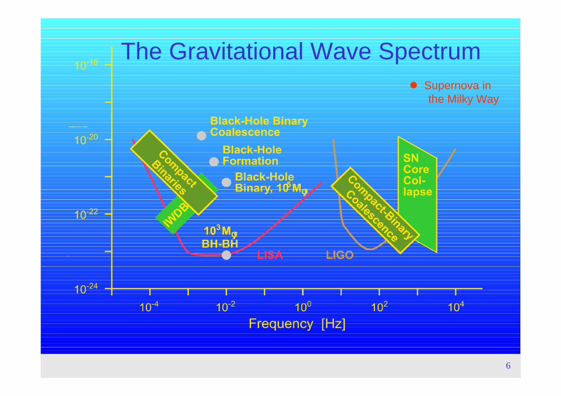
The Gravitational Wave SpectrumSupernova inthe Milky Way
7
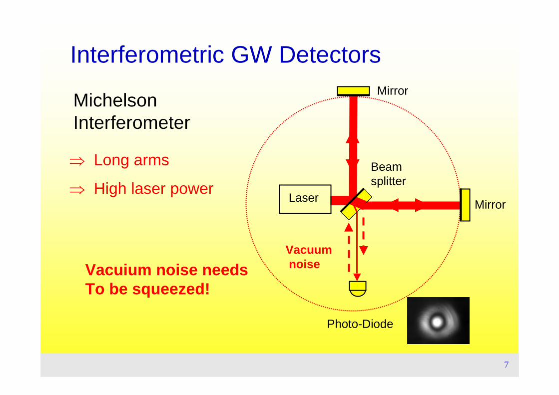
Laser
Photo-Diode
Beam splitter
Mirror
Mirror
⇒ Long arms
⇒ High laser power
Michelson Interferometer
Interferometric GW Detectors
VacuumnoiseVacuium noise needs
To be squeezed!
8
I. Introduction 2. Classical Interferometry
TopicsWaves and interferenceInterferometer topologiesThe beam splitterClassical description of the interferometerThe Michelson-Morley experiment
Literature• V. B. Braginski and F. Y. Khalili, Cambridge University Press (1995),
Quantum measurement. • P. R. Saulson, World Scientific (1994),
Fundamentals of Interferometric Gravitational Wave Detectors , 91 US$
9
∇2 v
E (v r ,t) −1c
∂2
∂t2
v E (v r ,t) = 0
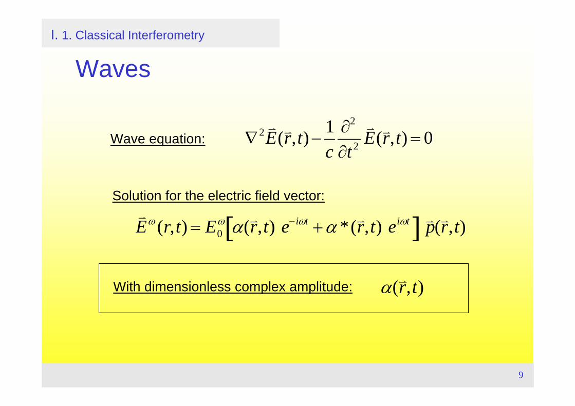
I. 1. Classical Interferometry
Waves
Wave equation:
Solution for the electric field vector:
v E ω (r,t) = E0
ω α(v r ,t) e−iωt + α *(v r ,t) eiωt[ ] v p (v r ,t)
α(v r ,t)With dimensionless complex amplitude:
10
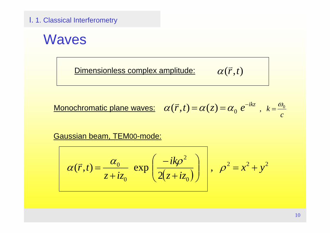
I. 1. Classical Interferometry
Waves
),( trvαDimensionless complex amplitude:
Monochromatic plane waves: ikzeztr −== 0)(),( ααα v
Gaussian beam, TEM00-mode:
( )222
0
2
0
0 ,2
exp),( yxizz
ikizz
tr +=⎟⎟⎠
⎞⎜⎜⎝
⎛+
−+
= ρραα v
ck 0, ω
=
11
0),(1),( 2
22 =
∂∂
−∇ trEtc
trE vvvv
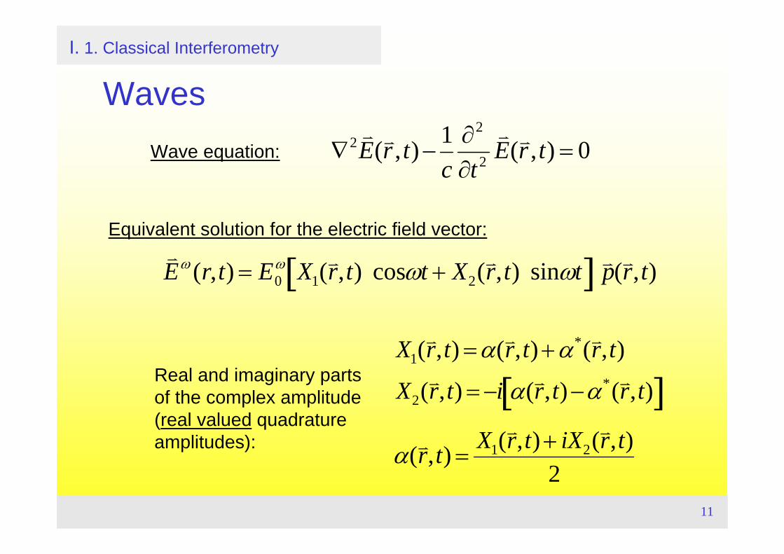
I. 1. Classical Interferometry
WavesWave equation:
Equivalent solution for the electric field vector:
v E ω (r,t) = E0
ω X1(v r ,t) cosωt + X2(
v r ,t) sinωt[ ] v p (v r ,t)
X1(v r ,t) =α(v r ,t) + α*(v r ,t)
X2(v r ,t) = −i α(v r ,t) −α*(v r ,t)[ ]
α(v r ,t) =X1(
v r ,t) + iX2(v r ,t)2
Real and imaginary parts of the complex amplitude (real valued quadrature amplitudes):
12
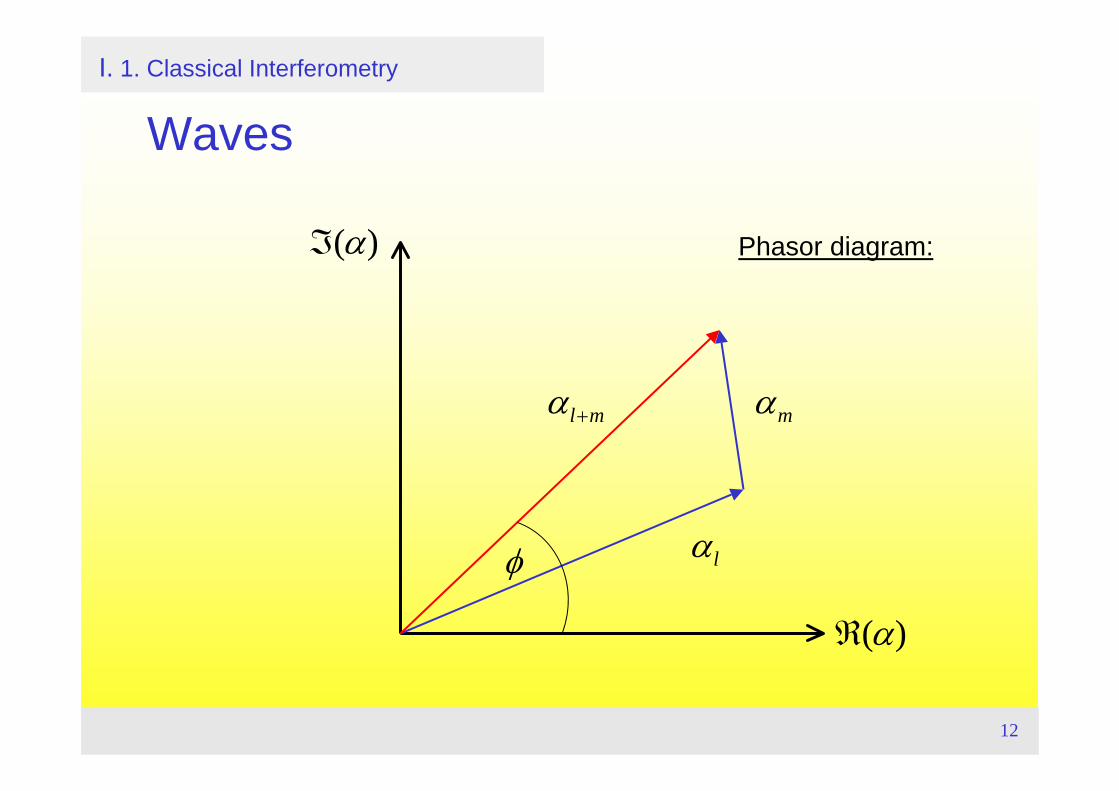
I. 1. Classical Interferometry
Waves
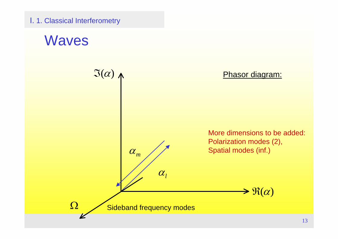
Phasor diagram:
ℜ(α)
ℑ(α)
lα
mαml+α
φ
13
I. 1. Classical Interferometry
Waves
Phasor diagram:
lα
mα
ℜ(α)
ℑ(α)
Ω Sideband frequency modes
More dimensions to be added:Polarization modes (2),Spatial modes (inf.)
14
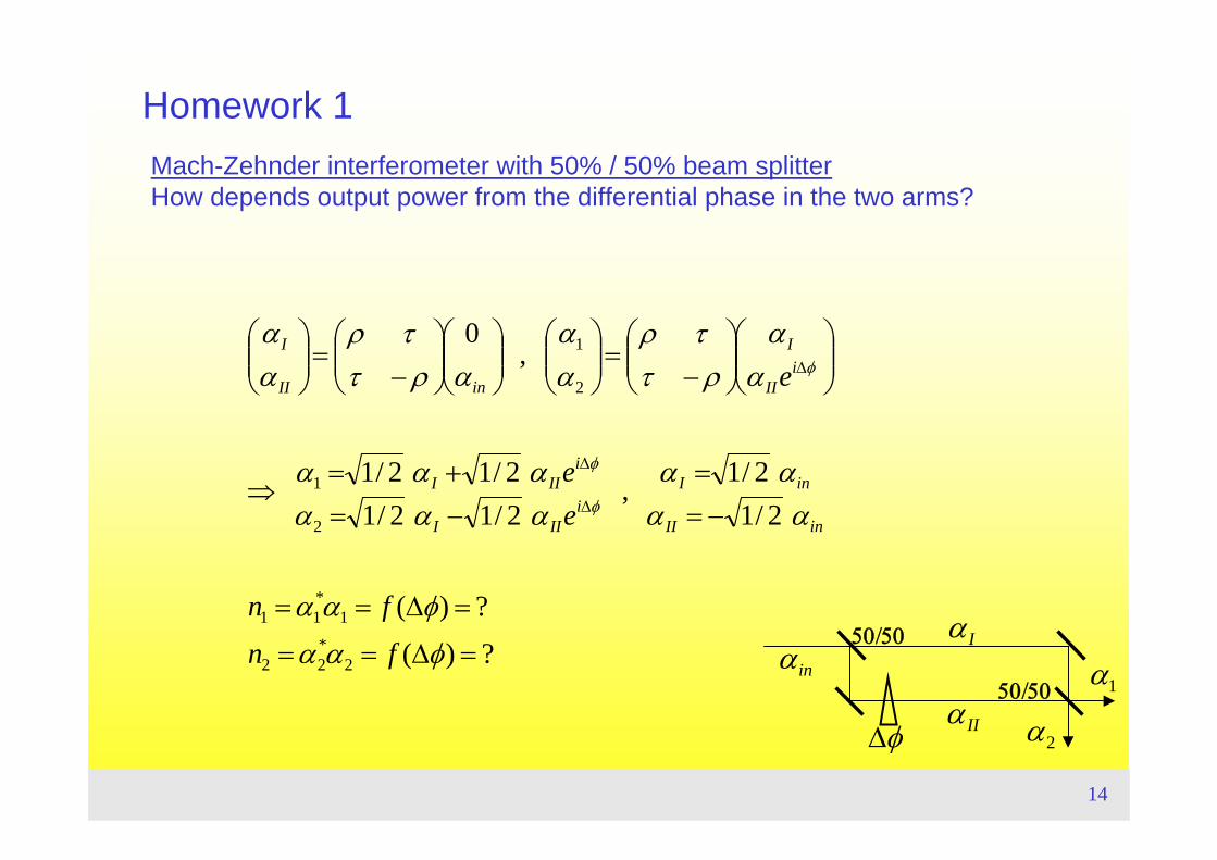
Homework 1Mach-Zehnder interferometer with 50% / 50% beam splitterHow depends output power from the differential phase in the two arms?
50/50
50/50inα
Iα
IIα1α
2αφΔ
?)(
?)(
2/12/1,
2/12/12/12/1
,0
2*22
1*11
2
1
2
1
=Δ==
=Δ==
−==
−=+=
⇒
⎟⎟⎠
⎞⎜⎜⎝
⎛⎟⎟⎠
⎞⎜⎜⎝
⎛−
=⎟⎟⎠
⎞⎜⎜⎝
⎛⎟⎟⎠
⎞⎜⎜⎝
⎛⎟⎟⎠
⎞⎜⎜⎝
⎛−
=⎟⎟⎠
⎞⎜⎜⎝
⎛
Δ
Δ
Δ
φαα
φαα
αααα
αααααα
αα
ρττρ
αα
αρττρ
αα
φ
φ
φ
fn
fn
ee
e
inII
inIi
III
iIII
iII
I
inII
I
15
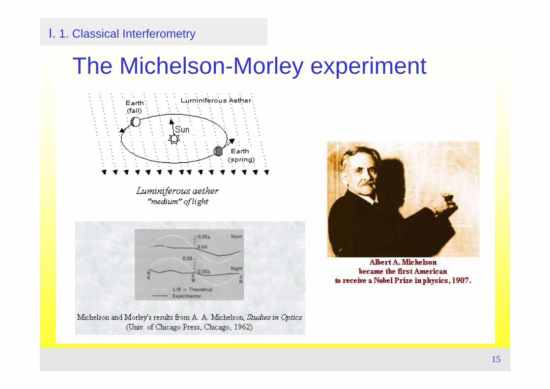
I. 1. Classical Interferometry
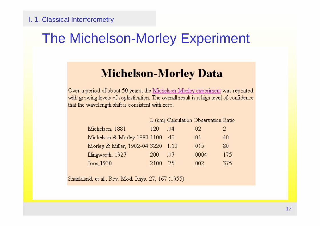
The Michelson-Morley experiment
16
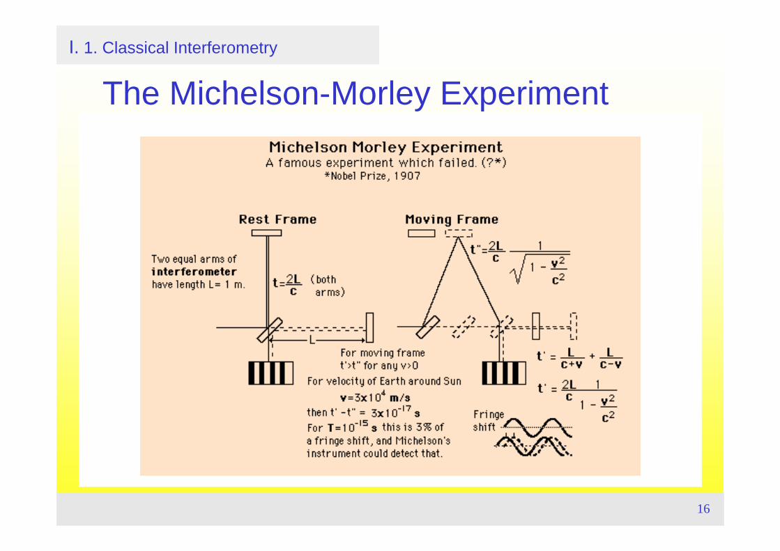
I. 1. Classical Interferometry
The Michelson-Morley Experiment
17
I. 1. Classical Interferometry
The Michelson-Morley Experiment
18
II. Interferometer Quantum Noise: Basics and Tools 3. Quantum Noise in Laser Interferometry
TopicsCoherent statesQuantum model of the beam splitter Quantum model of the interferometerShot noise
Literature• C. M. Caves, Phys. Rev. D 23, 1693 (1981),
Quantum-mechanical noise in an interferometer.• C. M. Caves and B. L. Schumaker, Phys. Rev. A 31, 3068 (1985),
New formalism for two-photon quantum optics.• V. B. Braginski and F. Y. Khalili, Cambridge University Press (1995),
Quantum measurement.
19
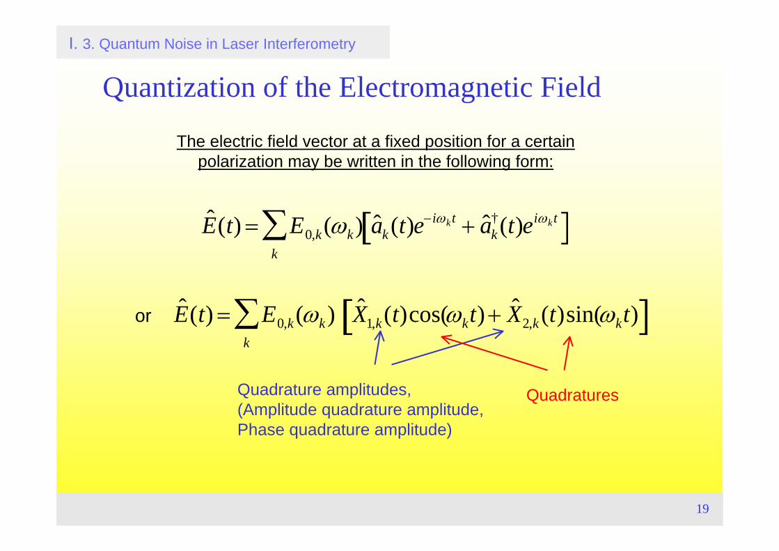
I. 3. Quantum Noise in Laser Interferometry
The electric field vector at a fixed position for a certain polarization may be written in the following form:
Quantization of the Electromagnetic Field
ˆ E (t) = E0,k(ωk) ˆ X 1,k(t)cos(ωkt) + ˆ X 2,k(t)sin(ωkt)[ ]k∑
QuadraturesQuadrature amplitudes,(Amplitude quadrature amplitude,Phase quadrature amplitude)
or
ˆ E (t) = E0,k(ωk) ˆ a k(t)e−iωkt + ˆ a k†(t)eiωkt[ ]
k∑
20
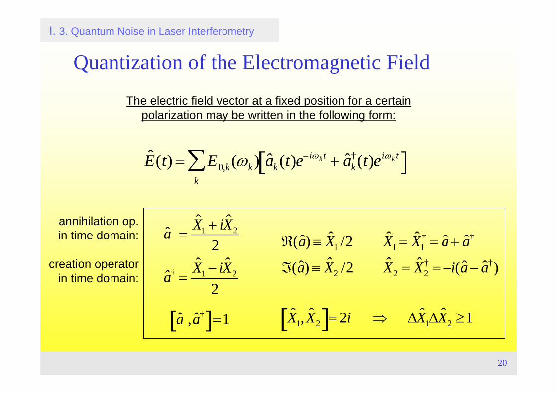
I. 3. Quantum Noise in Laser Interferometry
The electric field vector at a fixed position for a certain polarization may be written in the following form:
ˆ E (t) = E0,k(ωk) ˆ a k(t)e−iωkt + ˆ a k†(t)eiωkt[ ]
k∑
Quantization of the Electromagnetic Field
ˆ a =ˆ X 1 + i ˆ X 2
2
ˆ a † =ˆ X 1 − i ˆ X 2
2
ˆ a , ˆ a †[ ]=1
ℜ( ˆ a ) ≡ ˆ X 1 /2 ˆ X 1 = ˆ X 1† = ˆ a + ˆ a †
ℑ( ˆ a ) ≡ ˆ X 2 /2 ˆ X 2 = ˆ X 2† = −i( ˆ a − ˆ a †)
ˆ X 1, ˆ X 2[ ]= 2i ⇒ Δ ˆ X 1Δ ˆ X 2 ≥1
annihilation op. in time domain:
creation operator in time domain:
21
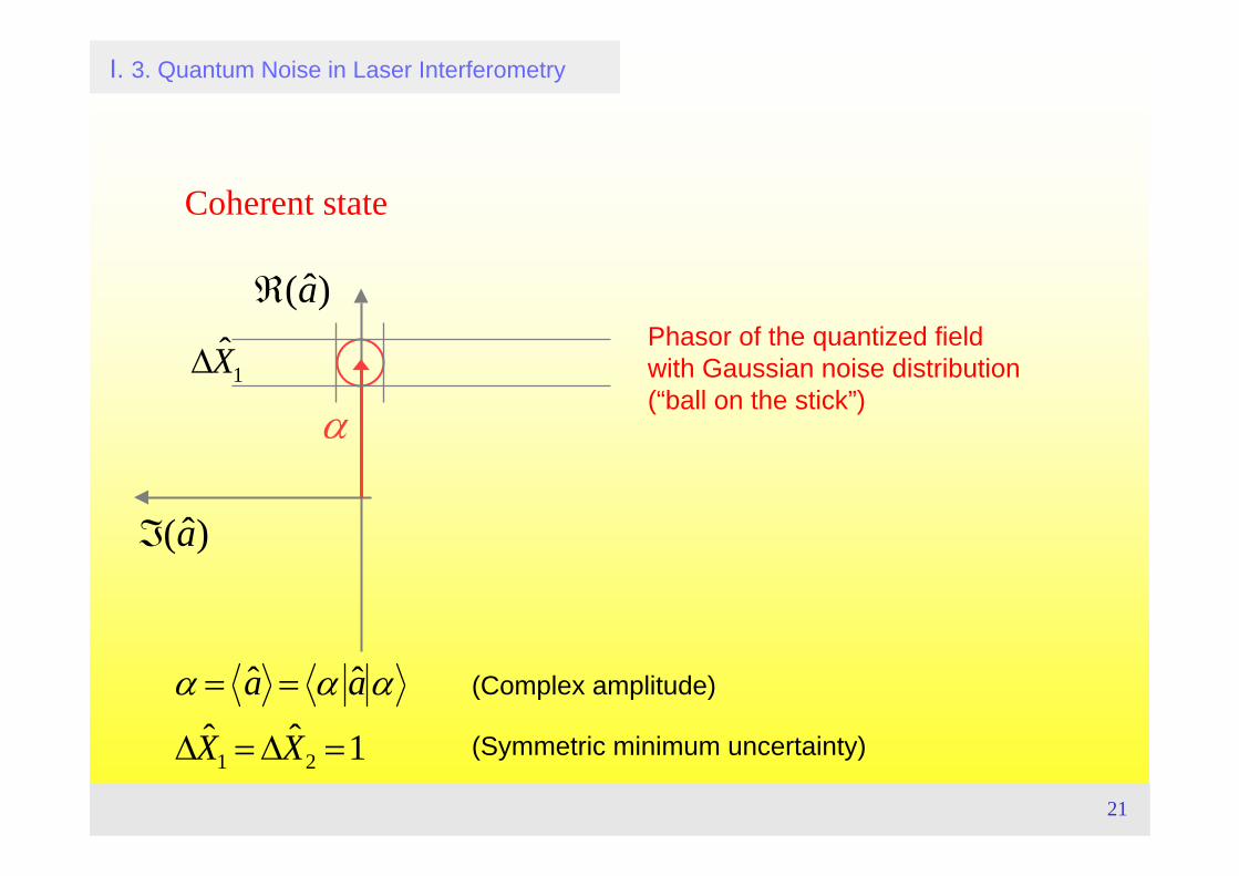
Coherent state
)ˆ(aℜ
)ˆ(aℑ
α
I. 3. Quantum Noise in Laser Interferometry
α = ˆ a = α ˆ a α
Δ ˆ X 1 = Δ ˆ X 2 =1
Δ ˆ X 1
(Complex amplitude)
(Symmetric minimum uncertainty)
Phasor of the quantized field with Gaussian noise distribution(“ball on the stick”)
22
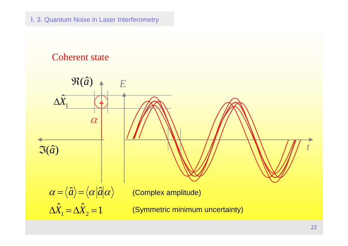
Coherent state
)ˆ(aℜ
)ˆ(aℑ
α
E
t
I. 3. Quantum Noise in Laser Interferometry
α = ˆ a = α ˆ a α
Δ ˆ X 1 = Δ ˆ X 2 =1
Δ ˆ X 1
(Complex amplitude)
(Symmetric minimum uncertainty)
23
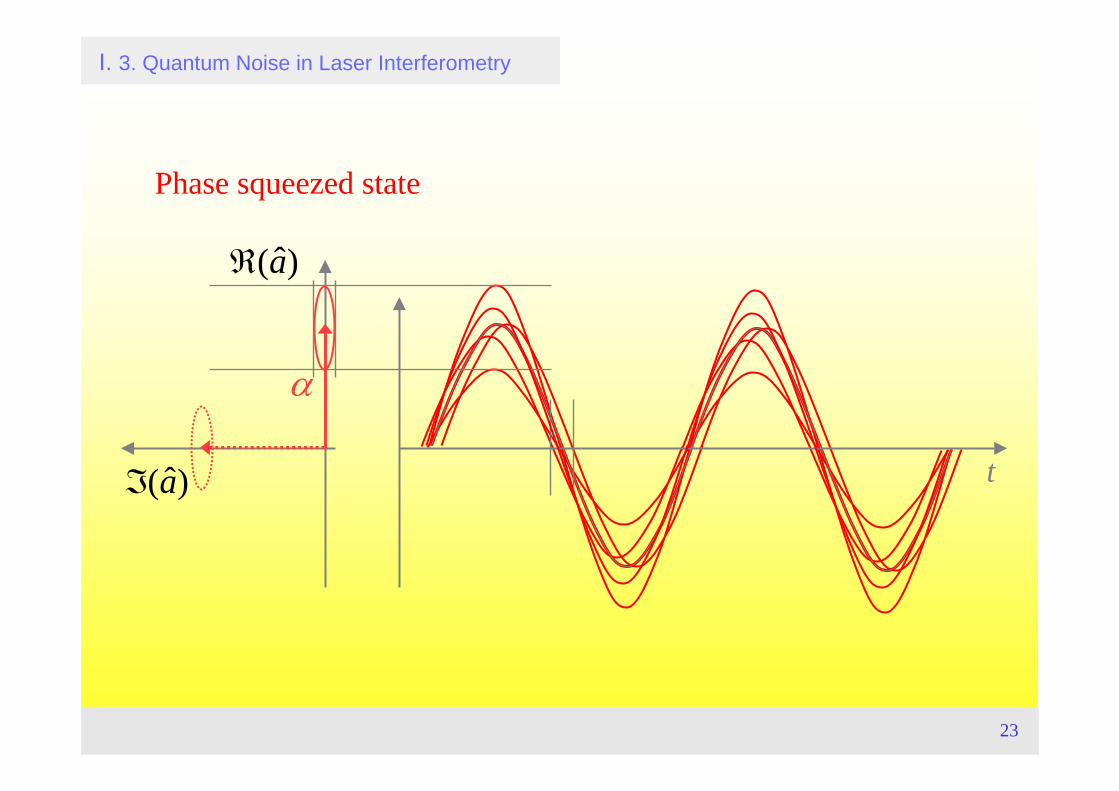
Phase squeezed state
I. 3. Quantum Noise in Laser Interferometry
t
)ˆ(aℜ
)ˆ(aℑ
α
24
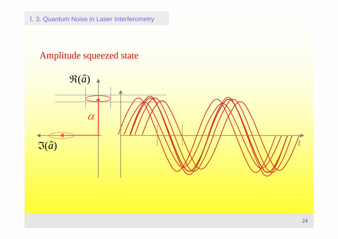
Amplitude squeezed state
I. 3. Quantum Noise in Laser Interferometry
t
)ˆ(aℜ
)ˆ(aℑ
α
25
I. 3. Quantum Noise in Laser Interferometry
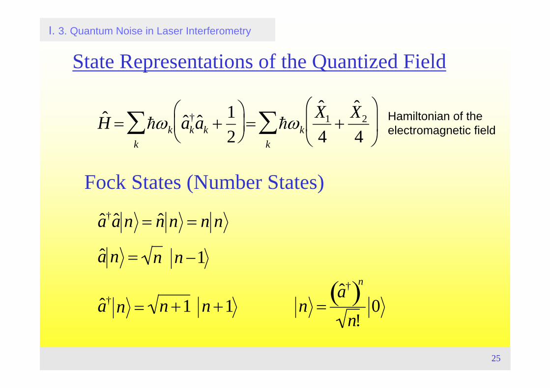
State Representations of the Quantized Field
Fock States (Number States)
ˆ H = hωkk
∑ ˆ a k† ˆ a k +
12
⎛ ⎝ ⎜
⎞ ⎠ ⎟ = hωk
k∑
ˆ X 14
+ˆ X 24
⎛
⎝ ⎜
⎞
⎠ ⎟
ˆ a † ˆ a n = ˆ n n = n n
ˆ a n = n n −1
ˆ a † n = n +1 n +1 n =ˆ a †( )n
n!0
Hamiltonian of the electromagnetic field
26
I. 3. Quantum Noise in Laser Interferometry
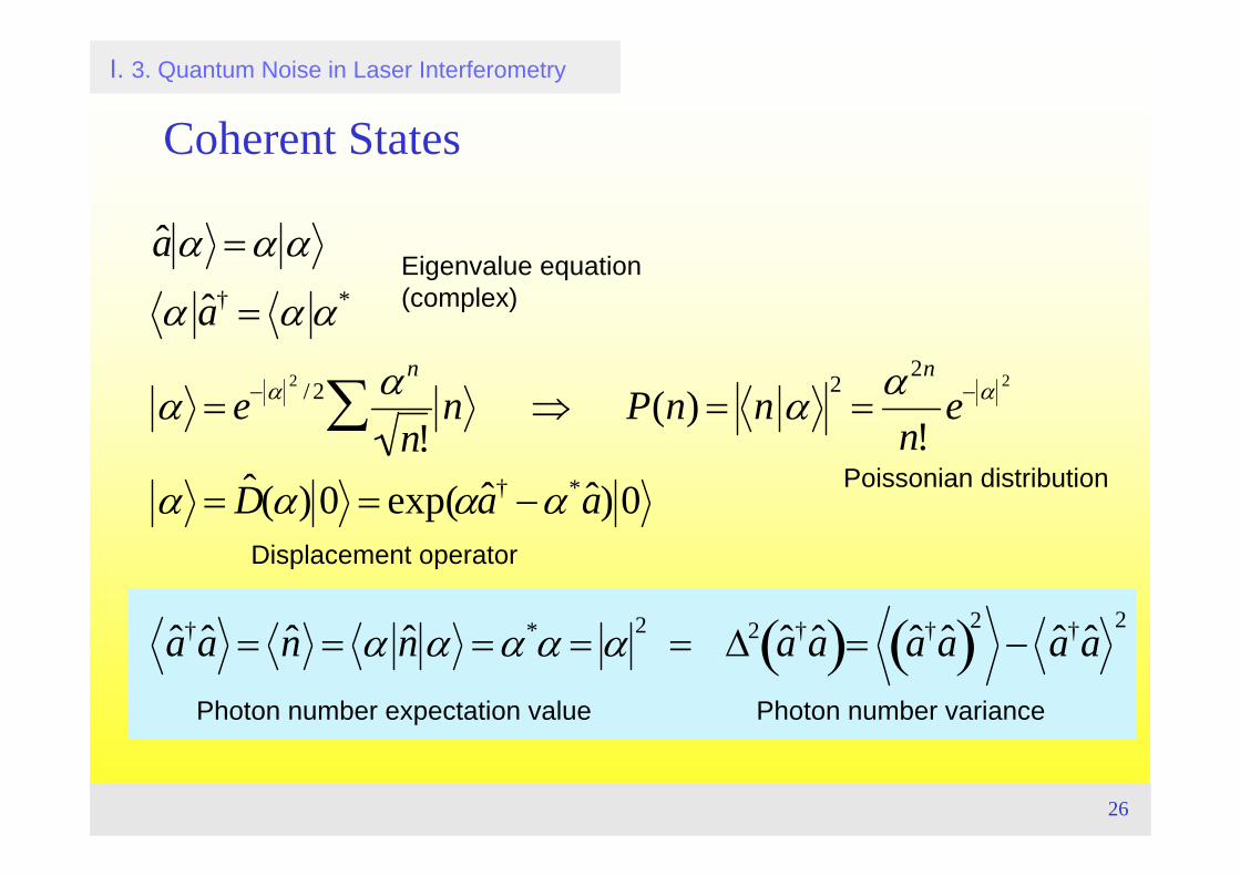
Coherent States
ˆ a α =α α
α ˆ a † = α α*
α = e− α 2 / 2 αn
n!∑ n ⇒ P(n) = n α
2=
α2n
n!e− α 2
α = ˆ D (α) 0 = exp(αˆ a † −α* ˆ a ) 0
ˆ a † ˆ a = ˆ n = α ˆ n α =α*α = α 2 = Δ2 ˆ a † ˆ a ( )= ˆ a † ˆ a ( )2− ˆ a † ˆ a
2
Eigenvalue equation (complex)
Displacement operator
Poissonian distribution
Photon number expectation value Photon number variance
27
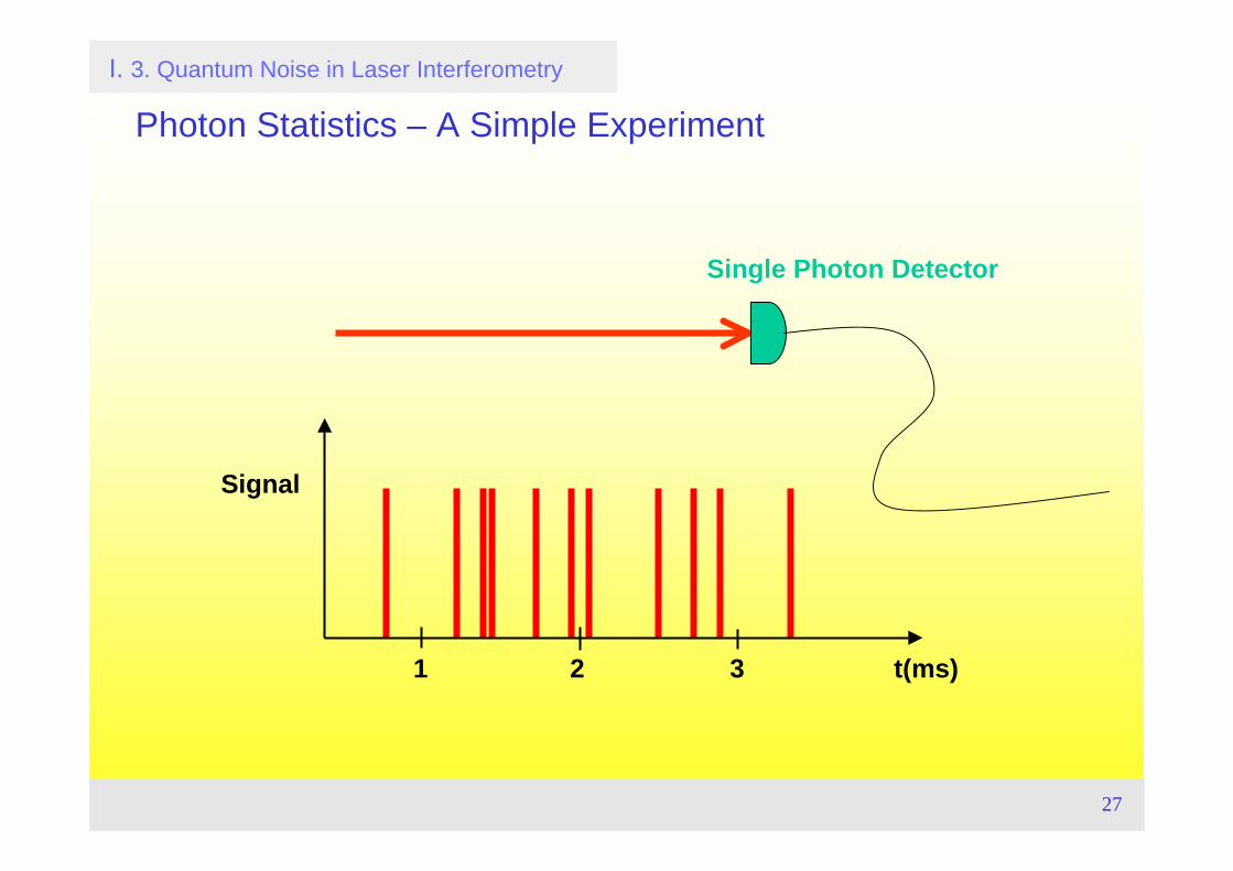
Photon Statistics – A Simple Experiment
I. 3. Quantum Noise in Laser Interferometry
1 2 3 t(ms)
Signal
Single Photon Detector
28
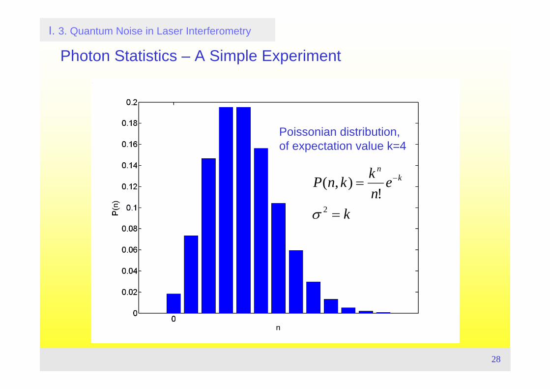
Photon Statistics – A Simple Experiment
I. 3. Quantum Noise in Laser Interferometry
Poissonian distribution, of expectation value k=4
k
enkknP k
n
=
= −
2
!),(
σ
29
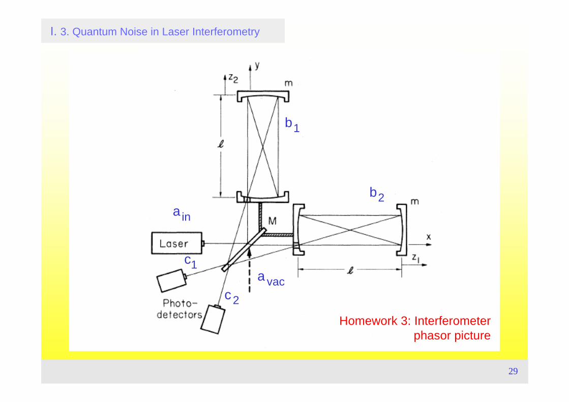
I. 3. Quantum Noise in Laser Interferometry
ina
vaca
2c
1 c
1b
2b
Homework 3: Interferometer phasor picture
30
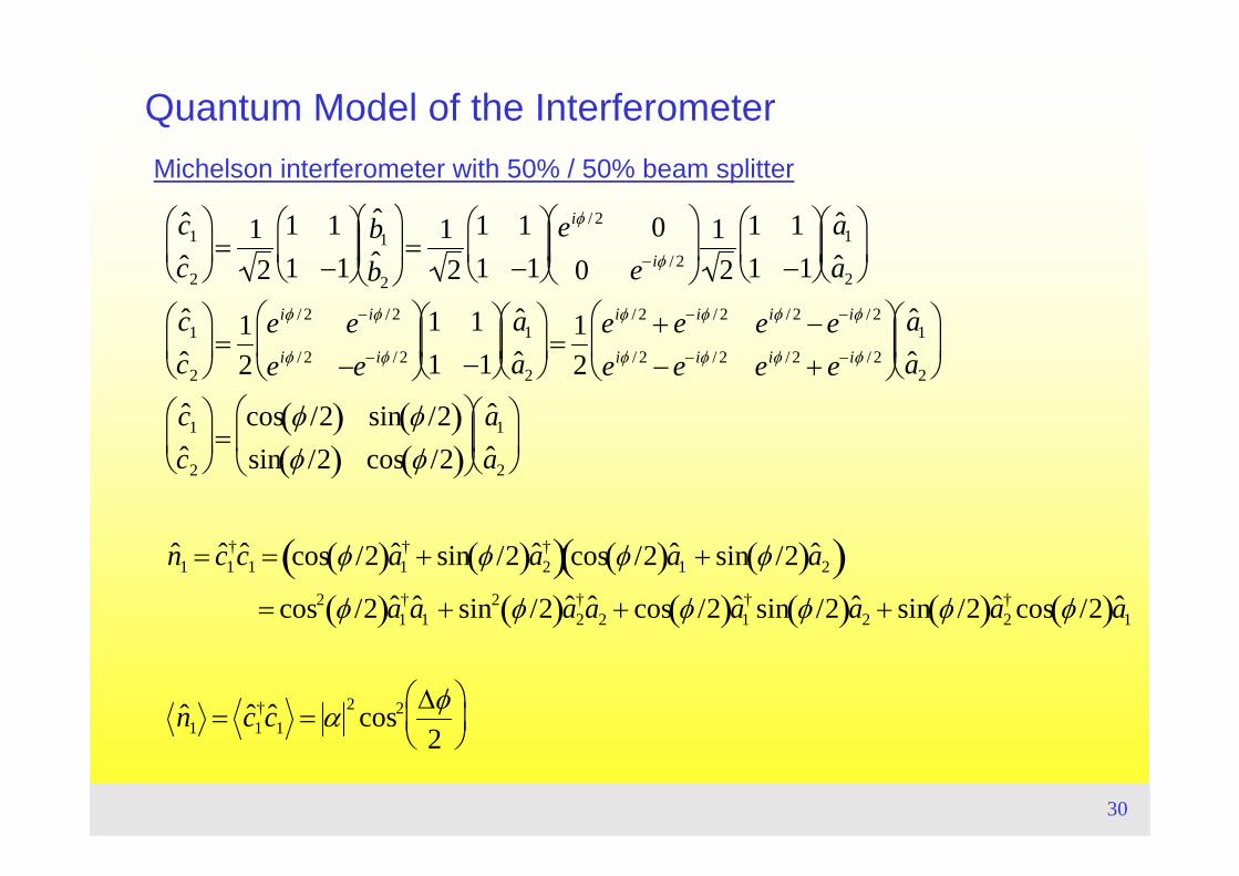
Quantum Model of the InterferometerMichelson interferometer with 50% / 50% beam splitter
ˆ c 1ˆ c 2
⎛
⎝ ⎜
⎞
⎠ ⎟ =
12
1 11 −1
⎛
⎝ ⎜
⎞
⎠ ⎟
ˆ b 1ˆ b 2
⎛
⎝ ⎜
⎞
⎠ ⎟ =
12
1 11 −1
⎛
⎝ ⎜
⎞
⎠ ⎟
eiφ / 2 00 e−iφ / 2
⎛
⎝ ⎜
⎞
⎠ ⎟
12
1 11 −1
⎛
⎝ ⎜
⎞
⎠ ⎟
ˆ a 1ˆ a 2
⎛
⎝ ⎜
⎞
⎠ ⎟
ˆ c 1ˆ c 2
⎛
⎝ ⎜
⎞
⎠ ⎟ =
12
eiφ / 2 e−iφ / 2
eiφ / 2 −e−iφ / 2
⎛
⎝ ⎜
⎞
⎠ ⎟
1 11 −1
⎛
⎝ ⎜
⎞
⎠ ⎟
ˆ a 1ˆ a 2
⎛
⎝ ⎜
⎞
⎠ ⎟ =
12
eiφ / 2 + e−iφ / 2 eiφ / 2 − e−iφ / 2
eiφ / 2 − e−iφ / 2 eiφ / 2 + e−iφ / 2
⎛
⎝ ⎜
⎞
⎠ ⎟
ˆ a 1ˆ a 2
⎛
⎝ ⎜
⎞
⎠ ⎟
ˆ c 1ˆ c 2
⎛
⎝ ⎜
⎞
⎠ ⎟ =
cos φ /2( ) sin φ /2( )sin φ /2( ) cos φ /2( )
⎛
⎝ ⎜
⎞
⎠ ⎟
ˆ a 1ˆ a 2
⎛
⎝ ⎜
⎞
⎠ ⎟
ˆ n 1 = ˆ c 1† ˆ c 1 = cos φ /2( )ˆ a 1
† + sin φ /2( )ˆ a 2†( )cos φ /2( )ˆ a 1 + sin φ /2( )ˆ a 2( )
= cos2 φ /2( )ˆ a 1† ˆ a 1 + sin2 φ /2( )ˆ a 2
† ˆ a 2 + cos φ /2( )ˆ a 1† sin φ /2( )ˆ a 2 + sin φ /2( )ˆ a 2
† cos φ /2( )ˆ a 1
ˆ n 1 = ˆ c 1† ˆ c 1 = α 2 cos2 Δφ
2⎛ ⎝ ⎜
⎞ ⎠ ⎟
31
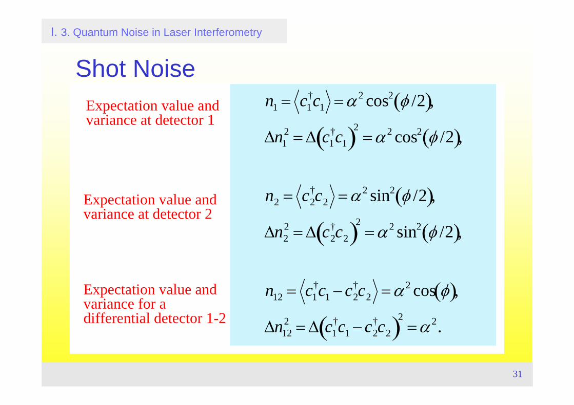
n1 = c1†c1 = α 2 cos2 φ /2( ),
Δn12 = Δ c1
†c1( )2= α 2 cos2 φ /2( ),
n2 = c2†c2 = α2 sin2 φ /2( ),
Δn22 = Δ c2
†c2( )2= α 2 sin2 φ /2( ),
n12 = c1†c1 − c2
†c2 = α2 cos φ( ),
Δn122 = Δ c1
†c1 − c2†c2( )2
= α 2.
I. 3. Quantum Noise in Laser Interferometry
Shot Noise
Expectation value and variance at detector 2
Expectation value and variance for a differential detector 1-2
Expectation value and variance at detector 1
32
I. 3. Quantum Noise in Laser Interferometry
Shot Noise
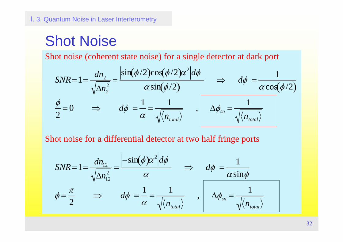
SNR =1=dn2
Δn22
=sin φ /2( )cos φ /2( )α 2 dφ
α sin φ /2( )⇒ dφ =
1α cos φ /2( )
φ2
= 0 ⇒ dφ =1α
=1
ntotal
, Δφsn =1
ntotal
SNR =1=dn12
Δn122
=−sin φ( )α 2 dφ
α⇒ dφ =
1α sinφ
φ =π2
⇒ dφ =1α
=1
ntotal
, Δφsn =1
ntotal
Shot noise (coherent state noise) for a single detector at dark port
Shot noise for a differential detector at two half fringe ports
33
II. Interferometer Quantum Noise: Basics and Tools 4. Quantum Noise Spectral Densities
TopicsNoise spectral densities:
Shot noiseRadiation pressure noiseStandard Quantum Limit (SQL)
GEO 600
Literature• H. A. Haus, Electromagnetic Noise and Quantum Optical Measurement,
Springer, Berlin (2000)• C. Kittel, Elementary Statistical Physics, Wiley, New York (1958),• F. Reif, Fundamentals of Statistical Physics, McGraw-Hill, New York (1965),• H-A. Bachor and T. Ralph, Guide to Experiments in Quantum Optics,
Springer, Berlin (2003),• P. R. Saulson, World Scientific (1994),
Fundamentals of Interferometric Gravitational Wave Detectors.
34
I. 4. Quantum Noise Spectral Densities
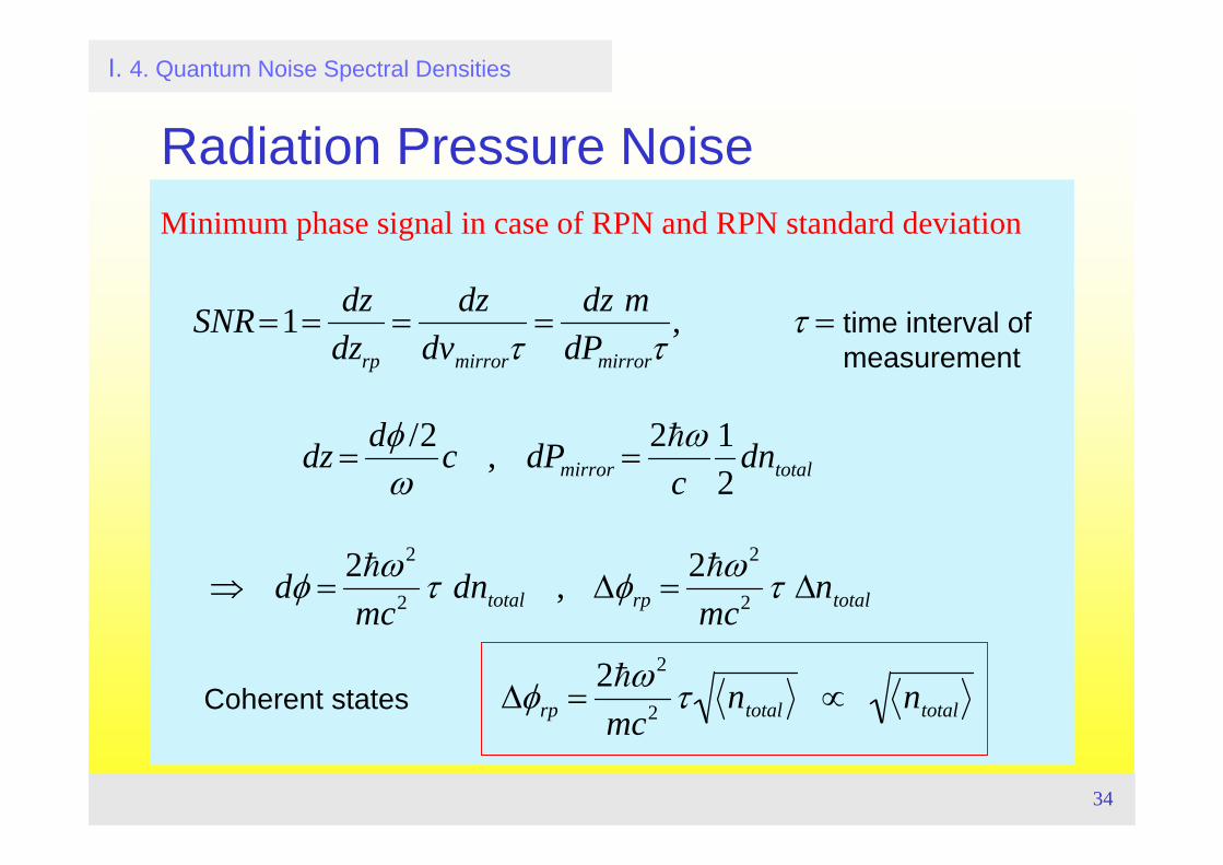
Radiation Pressure Noise
SNR =1=dz
dzrp
=dz
dvmirrorτ=
dz mdPmirrorτ
, τ =
dz =dφ /2
ωc , dPmirror =
2hωc
12
dntotal
⇒ dφ =2hω2
mc2 τ dntotal , Δφrp =2hω2
mc2 τ Δntotal
Δφrp =2hω2
mc2 τ ntotal ∝ ntotal
Minimum phase signal in case of RPN and RPN standard deviation
time interval ofmeasurement
Coherent states
35
I. 4. Quantum Noise Spectral Densities
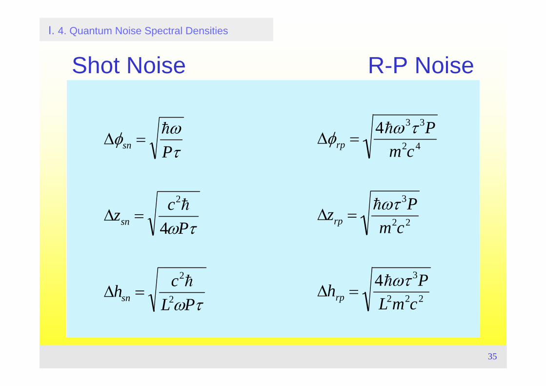
Shot Noise R-P Noise
τω
τω
τωφ
PLch
Pcz
P
sn
sn
sn
2
2
2
4
h
h
h
=Δ
=Δ
=Δ
Δφrp =4hω3τ 3P
m2c4
Δzrp =hωτ 3Pm2c2
Δhrp =4hωτ 3PL2m2c2
36
I. 4. Quantum Noise Spectral Densities
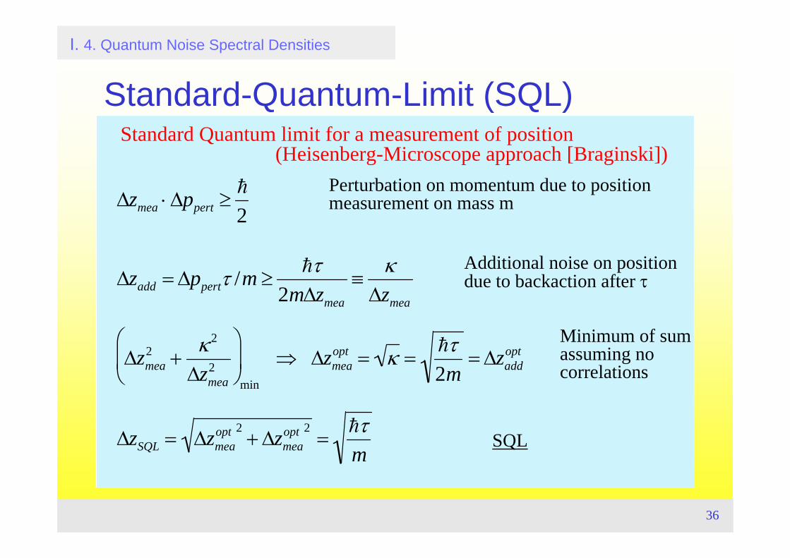
Standard-Quantum-Limit (SQL)
Δzmea ⋅ Δppert ≥h
2
Δzadd = Δppertτ /m ≥hτ
2mΔzmea
≡κ
Δzmea
Δzmea2 +
κ 2
Δzmea2
⎛
⎝ ⎜
⎞
⎠ ⎟
min
⇒ Δzmeaopt = κ =
hτ2m
= Δzaddopt
ΔzSQL = Δzmeaopt 2
+ Δzmeaopt 2
=hτm
Standard Quantum limit for a measurement of position(Heisenberg-Microscope approach [Braginski])
Perturbation on momentum due to positionmeasurement on mass m
Additional noise on positiondue to backaction after τ
Minimum of sum assuming no correlations
SQL
37
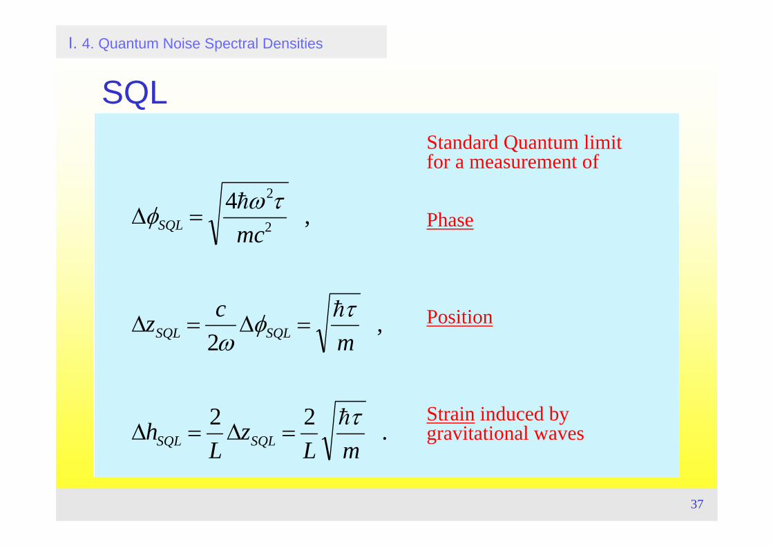
I. 4. Quantum Noise Spectral Densities
SQL
.22
,2
,42
2
mLz
Lh
mcz
mc
SQLSQL
SQLSQL
SQL
τ
τφω
τωφ
h
h
h
=Δ=Δ
=Δ=Δ
=Δ
Standard Quantum limit for a measurement of
Phase
Position
Strain induced by gravitational waves
38
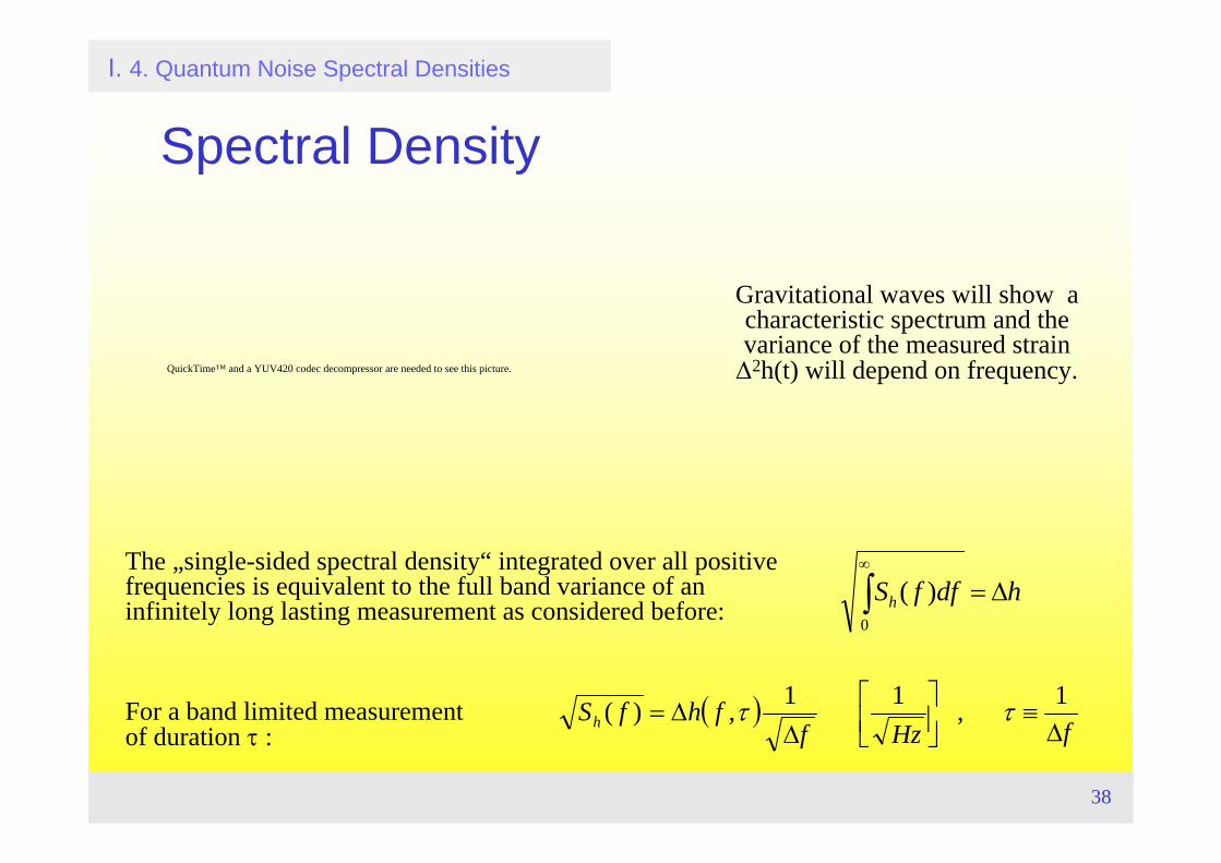
The „single-sided spectral density“ integrated over all positive frequencies is equivalent to the full band variance of an infinitely long lasting measurement as considered before:
For a band limited measurement of duration τ :
I. 4. Quantum Noise Spectral Densities
Spectral Density
QuickTime™ and a YUV420 codec decompressor are needed to see this picture.
hdffSh Δ=∫∞
0
)(
( )fHzf
fhfSh Δ≡⎥⎦
⎤⎢⎣
⎡Δ
Δ=1,11,)( ττ
Gravitational waves will show a characteristic spectrum and the variance of the measured strain
Δ2h(t) will depend on frequency.
39
I. 4. Quantum Noise Spectral Densities
Spectral Density
( )( )
( ) ( ) hhhhhC
dththhthT
C
dtthT
h
hh
n
T
TTn
T
TT
22___________
2
2/
2/
2/
2/
)0(
)()(1lim)(
)(1lim
Δ≡−=−=⇒
−+−≡
≡
=
∫
∫
+
−∞→
+
−∞→
ττ
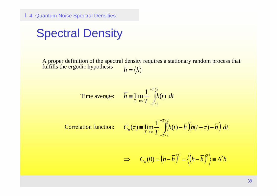
Time average:
Correlation function:
A proper definition of the spectral density requires a stationary random process that fulfills the ergodic hypothesis
40
I. 4. Quantum Noise Spectral Densities
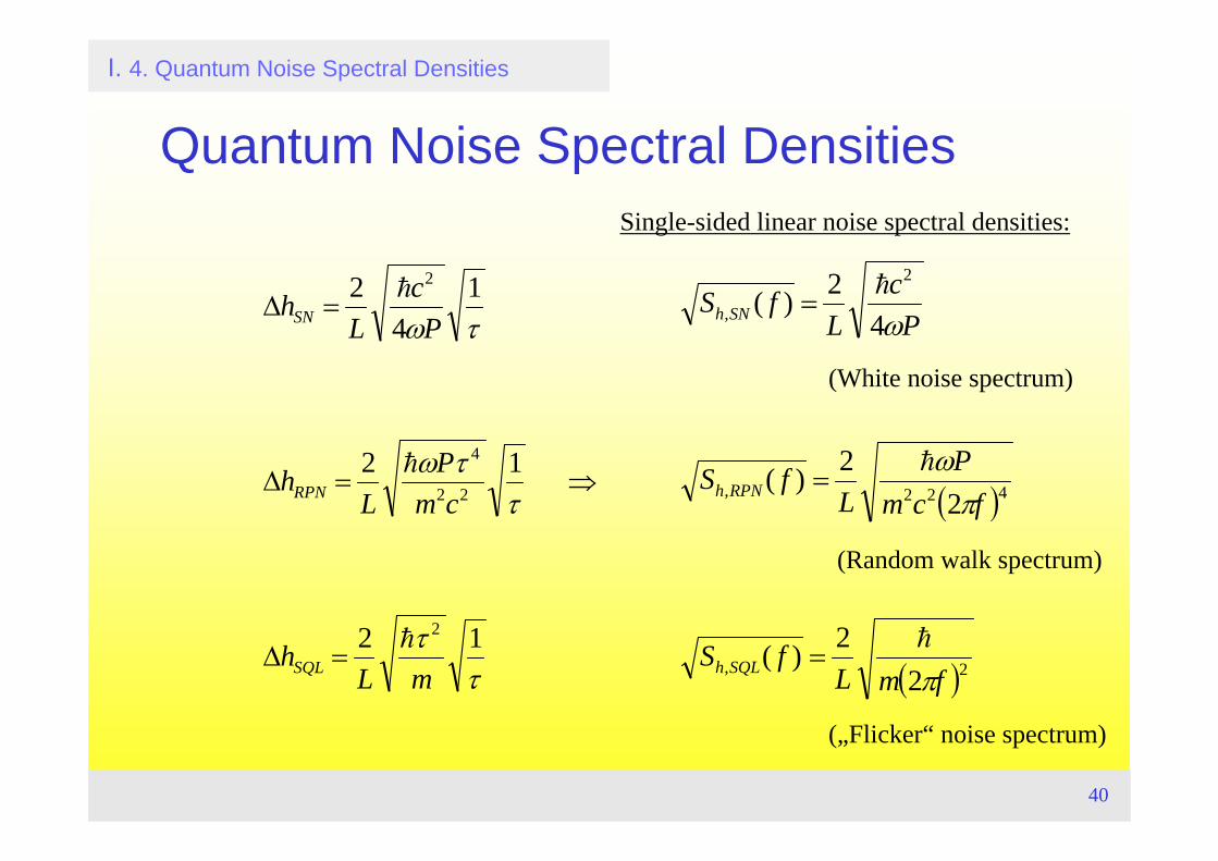
Quantum Noise Spectral DensitiesSingle-sided linear noise spectral densities:
( )
( )2,
422,
2
,
22)(
22)(
42)(
fmLfS
fcmP
LfS
Pc
LfS
SQLh
RPNh
SNh
π
πω
ω
h
h
h
=
=
=
ττ
ττω
τω
12
12
14
2
2
22
4
2
mLh
cmP
Lh
Pc
Lh
SQL
RPN
SN
h
h
h
=Δ
⇒=Δ
=Δ
(White noise spectrum)
(Random walk spectrum)
(„Flicker“ noise spectrum)
41
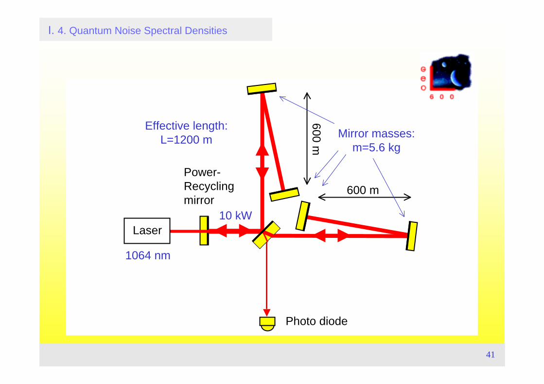
I. 4. Quantum Noise Spectral Densities
Power-Recyclingmirror
Laser
Photo diode
600 m
600 m
1064 nm
Mirror masses:m=5.6 kg
Effective length:L=1200 m
10 kW
42
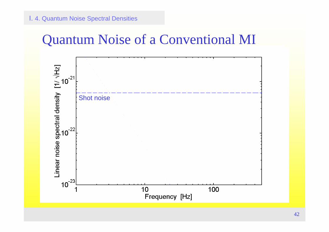
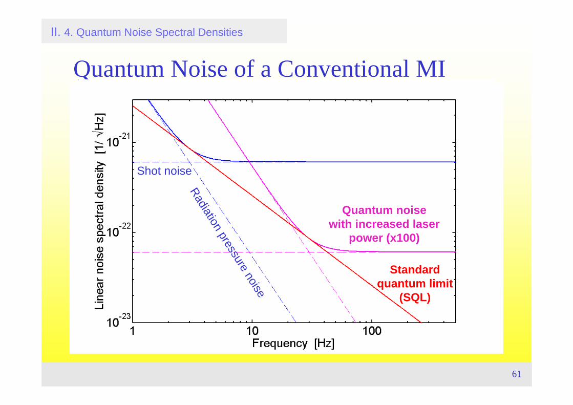
Quantum Noise of a Conventional MI
Shot noise
I. 4. Quantum Noise Spectral Densities

43
Quantum noise in phase quadrature
Quantum Noise of a Conventional MI
Standard quantum limit
(SQL)
Quantum noisewith increased laser
power (x100)
Shot noise
Radiation pressure noise
I. 4. Quantum Noise Spectral Densities
44
II. Interferometer Quantum Noise: Basics and Tools 5. Interferometer Readout:
Homodyne versus Heterodyne Detection
TopicsBalanced homodyne detection Homodyne detection in gravitational wave interferometersModulation/demodulation technique: heterodyne detectionBalanced sideband heterodyne detectionUnbalanced sideband heterodyne detectionQuantum noise in homodyne and heterodyne detection
Literature• A. Buonanno, Y. Chen, and N. Mavalvala, Phys. Rev. D 67, 122005 (2003),
Quantum noise in laser-interferometer gravitational-wave detectors with a heterodyne readout scheme.

45
(Squeezed) signal beamIntense local
oscillator
Phase shift θ
Electric current
V(ˆ i −) ≅ αLO2 ⋅ δ ˆ X 1 cosθ +δ ˆ X 2 sinθ
2= αLO
2 ⋅ δ ˆ X θ2 ≡ αLO
2 ⋅ Δ2 ˆ X θ
Balanced Homodyne Detection
Interf
ering
50/50
beam
splitte
r
II. 5. Homodyne versus heterodyne detection
ab
NaEa
46
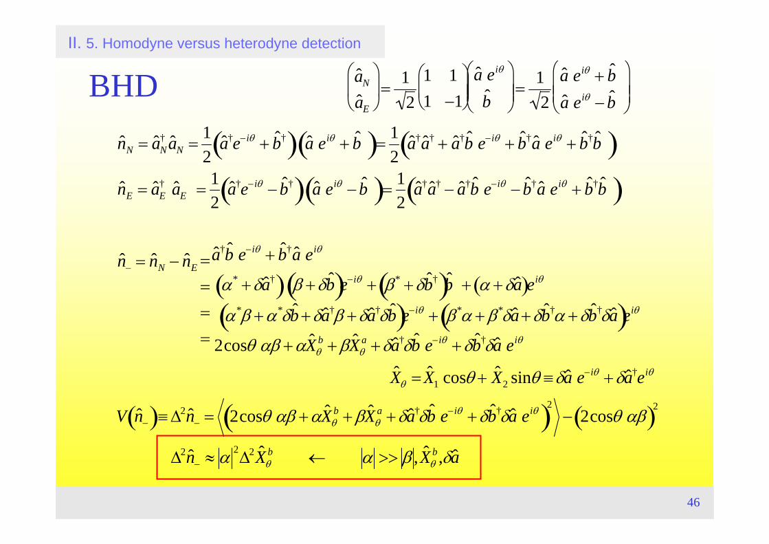
BHDII. 5. Homodyne versus heterodyne detection
ˆ a Nˆ a E
⎛
⎝ ⎜
⎞
⎠ ⎟ =
12
1 11 −1
⎛
⎝ ⎜
⎞
⎠ ⎟
ˆ a eiθ
ˆ b
⎛
⎝ ⎜ ⎜
⎞
⎠ ⎟ ⎟ =
12
ˆ a eiθ + ˆ b ˆ a eiθ − ˆ b
⎛
⎝ ⎜ ⎜
⎞
⎠ ⎟ ⎟
ˆ n N = ˆ a N† ˆ a N =
12
ˆ a †e−iθ + ˆ b †( ) ˆ a eiθ + ˆ b ( )=12
ˆ a † ˆ a † + ˆ a † ˆ b e−iθ + ˆ b † ˆ a eiθ + ˆ b † ˆ b ( )ˆ n E = ˆ a E
† ˆ a E =12
ˆ a †e−iθ − ˆ b †( ) ˆ a eiθ − ˆ b ( )=12
ˆ a † ˆ a † − ˆ a † ˆ b e−iθ − ˆ b † ˆ a eiθ + ˆ b † ˆ b ( )
ˆ n − = ˆ n N − ˆ n E ====
ˆ a † ˆ b e−iθ + ˆ b † ˆ a eiθ
α* + δˆ a †( ) β + δ ˆ b ( )e−iθ + β* + δ ˆ b †( ) b + α + δˆ a ( )eiθ
α*β + α*δ ˆ b + δˆ a †β + δˆ a †δ ˆ b ( )e−iθ + β*α + β*δˆ a + δ ˆ b †α + δ ˆ b †δˆ a ( )eiθ
2cosθ αβ + α ˆ X θb + β ˆ X θ
a + δˆ a †δ ˆ b e−iθ + δ ˆ b †δˆ a eiθ
ˆ X θ = ˆ X 1 cosθ + ˆ X 2 sinθ ≡ δˆ a e−iθ + δˆ a †eiθ
V ˆ n −( )≡ Δ2 ˆ n − = 2cosθ αβ + α ˆ X θb + β ˆ X θ
a + δˆ a †δ ˆ b e−iθ + δ ˆ b †δˆ a eiθ( )2− 2cosθ αβ( )2
Δ2 ˆ n − ≈ α 2Δ2 ˆ X θb ← α >> β , ˆ X θ
b,δˆ a
47
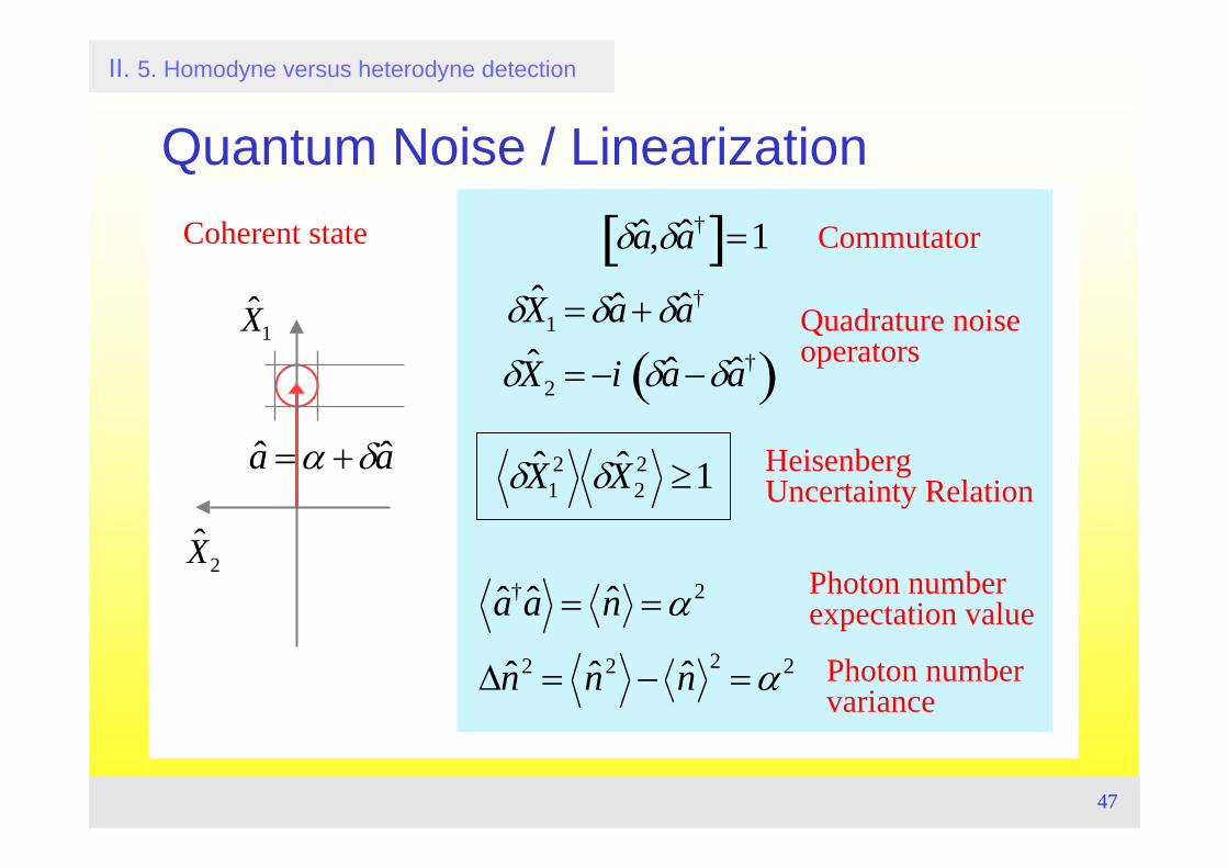
II. 5. Homodyne versus heterodyne detection
Quantum Noise / LinearizationCoherent state
E
t
ˆ X 1
ˆ X 2
aa ˆˆ δα +=
δ ˆ X 1 = δˆ a + δˆ a †
δ ˆ X 2 = −i δˆ a −δˆ a †( )
δˆ a ,δˆ a †[ ]=1
ˆ a † ˆ a = ˆ n = α 2
Δˆ n 2 = ˆ n 2 − ˆ n 2 = α 2
Quadrature noise operators
Commutator
Photon number expectation value
Photon number variance
δ ˆ X 12 δ ˆ X 2
2 ≥1 Heisenberg Uncertainty Relation
48
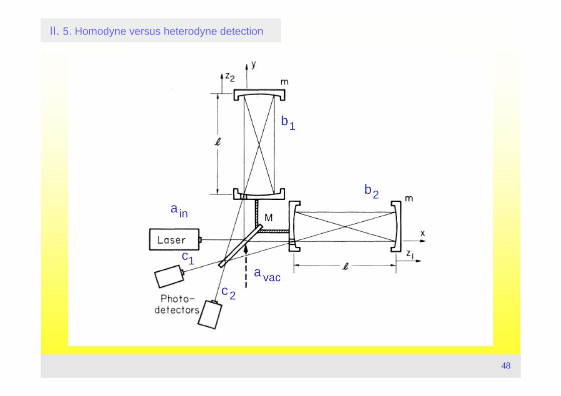
II. 5. Homodyne versus heterodyne detection
ina
vaca
2c
1 c
1b
2b

49
n1 = c1†c1 = α 2 cos2 φ /2( ),
Δn12 = Δ c1
†c1( )2= α 2 cos2 φ /2( ),
n2 = c2†c2 = α2 sin2 φ /2( ),
Δn22 = Δ c2
†c2( )2= α 2 sin2 φ /2( ),
n12 = c1†c1 − c2
†c2 = α2 cos φ( ),
Δn122 = Δ c1
†c1 − c2†c2( )2
= α 2.
I. 3. Quantum Noise in Laser Interferometry
Shot Noise
Expectation value and variance at detector 2
Expectation value and variance for a differential detector 1-2
Expectation value and variance at detector 1
50
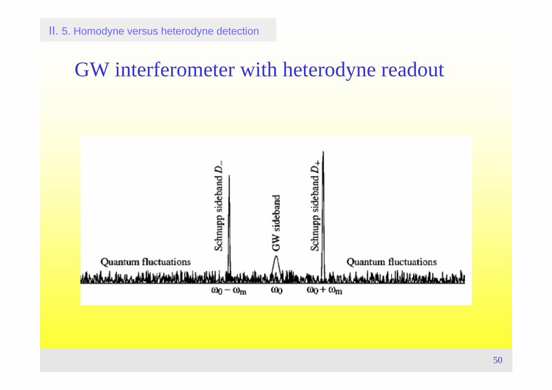
II. 5. Homodyne versus heterodyne detection
GW interferometer with heterodyne readout
51
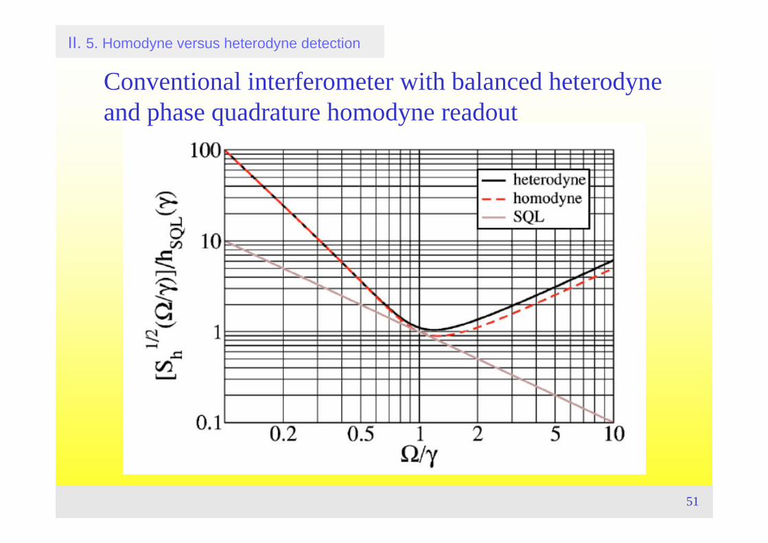
II. 5. Homodyne versus heterodyne detection
Conventional interferometer with balanced heterodyne and phase quadrature homodyne readout
52
II. Interferometer Quantum Noise: Basics and Tools 6. Quantum Noise of Sideband Modulation Fields
TopicsSideband modulations and quadrature fields„One-photon“ versus „Two-photon“ quantum opticsQuadrature noise operators in frequency domainCoherent and squeezed noisePhasor diagram in frequency domain
Literature• C. M. Caves, Phys. Rev. Lett. 31, 3068 (1985),
New Formalism for two-photon quantum optics.• H. J. Kimble, Y. Levin, A. B. Matsko, K. S. Thorne, and S. P. Vyatchanin,
Phys. Rev. D 65, 022002 (2001), Conversion of conventional gravitational-wave interferometers into quantum nondemolition interferometers by modifying their input and/or output optics.
53
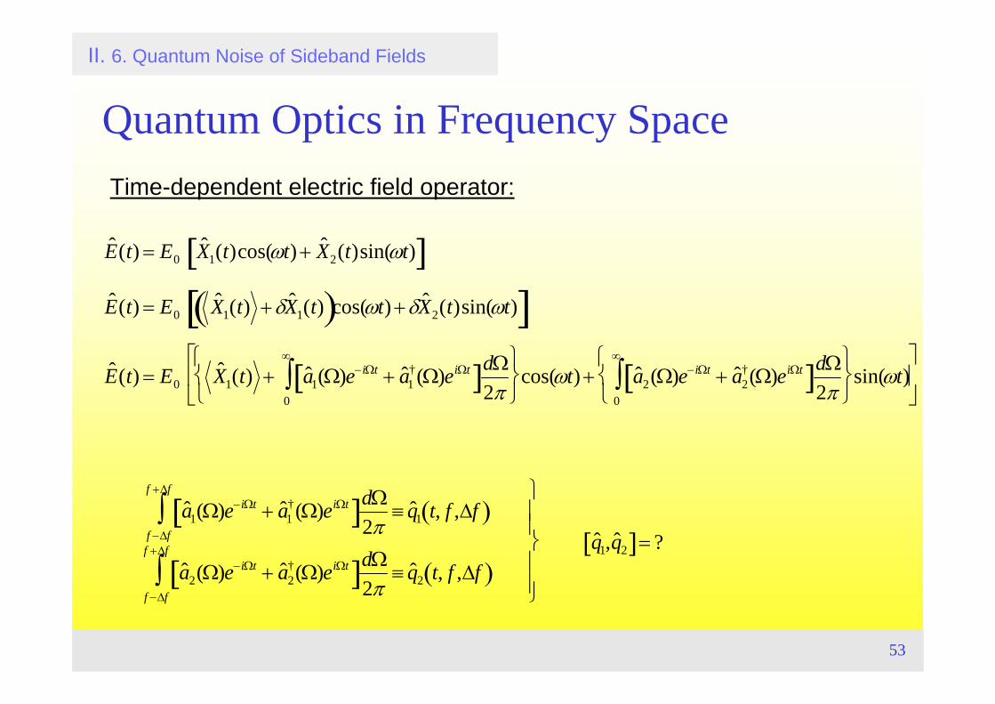
II. 6. Quantum Noise of Sideband Fields
Quantum Optics in Frequency SpaceTime-dependent electric field operator:
ˆ E (t) = E0ˆ X 1(t)cos(ωt) + ˆ X 2(t)sin(ωt)[ ]
ˆ E (t) = E0ˆ X 1(t) +δ ˆ X 1(t)( )cos(ωt) +δ ˆ X 2(t)sin(ωt)[ ]
ˆ E (t) = E0ˆ X 1(t) + ˆ a 1(Ω)e−iΩt + ˆ a 1
†(Ω)eiΩt[ ]dΩ2π0
∞
∫⎧ ⎨ ⎩
⎫ ⎬ ⎭
cos(ωt) + ˆ a 2(Ω)e−iΩt + ˆ a 2†(Ω)eiΩt[ ]dΩ
2π0
∞
∫⎧ ⎨ ⎩
⎫ ⎬ ⎭
sin(ωt)⎡
⎣ ⎢
⎤
⎦ ⎥
ˆ a 1(Ω)e−iΩt + ˆ a 1†(Ω)eiΩt[ ]dΩ
2πf −Δf
f +Δf
∫ ≡ ˆ q 1 t, f ,Δf( )
ˆ a 2(Ω)e−iΩt + ˆ a 2†(Ω)eiΩt[ ]dΩ
2πf −Δf
f +Δf
∫ ≡ ˆ q 2 t, f ,Δf( )
⎫
⎬ ⎪ ⎪
⎭ ⎪ ⎪
ˆ q 1, ˆ q 2[ ]= ?
54
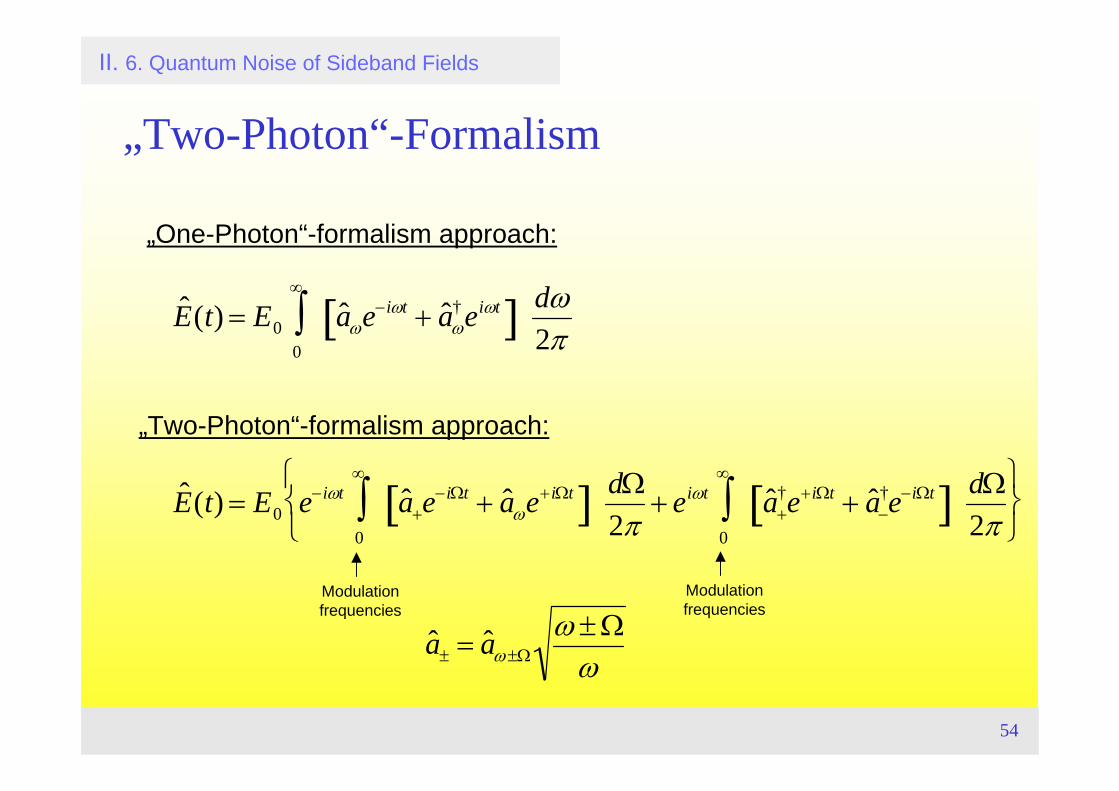
II. 6. Quantum Noise of Sideband Fields
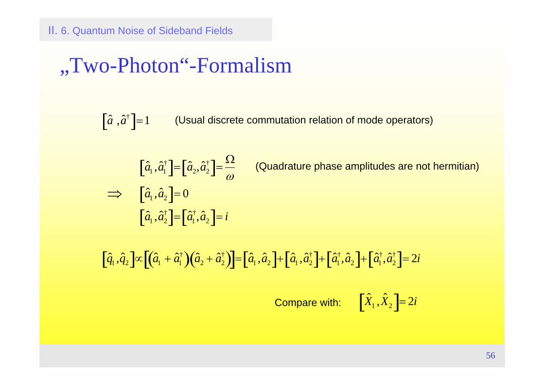
„Two-Photon“-Formalism
„One-Photon“-formalism approach:
„Two-Photon“-formalism approach:
ˆ E (t) = E0 ˆ a ωe−iωt + ˆ a ω† eiωt[ ] dω
2π0
∞
∫
ˆ E (t) = E0 e−iωt ˆ a +e−iΩt + ˆ a ωe+iΩt[ ] dΩ
2π0
∞
∫ + eiωt ˆ a +†e+iΩt + ˆ a −
†e−iΩt[ ] dΩ2π0
∞
∫⎧ ⎨ ⎩
⎫ ⎬ ⎭
ˆ a ± = ˆ a ω ±Ωω ± Ω
ω
Modulation frequencies
Modulation frequencies
55
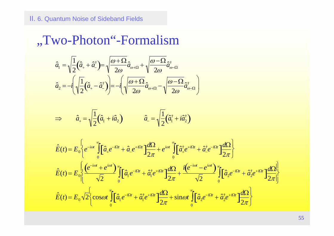
II. 6. Quantum Noise of Sideband Fields
„Two-Photon“-Formalismˆ a 1 = 1
2ˆ a + + ˆ a −
†( )= ω + Ω2ω
ˆ a ω +Ω + ω − Ω2ω
ˆ a ω−Ω†
ˆ a 2 = −i 12
ˆ a + − ˆ a −†( )
⎛
⎝ ⎜
⎞
⎠ ⎟ = −i ω + Ω
2ωˆ a ω +Ω −
ω − Ω2ω
ˆ a ω−Ω†
⎛
⎝ ⎜
⎞
⎠ ⎟
⇒ ˆ a + =12
ˆ a 1 + iˆ a 2( ) ˆ a − =12
ˆ a 1† + iˆ a 2
†( )
ˆ E (t) = E0 e−iωt ˆ a +e−iΩt + ˆ a −e
+iΩt[ ]dΩ2π0
∞
∫ + eiωt ˆ a +†e+iΩt + ˆ a −
†e−iΩt[ ]dΩ2π0
∞
∫⎧ ⎨ ⎩
⎫ ⎬ ⎭
ˆ E (t) = E0
e−iωt + eiωt( )2
ˆ a 1e−iΩt + ˆ a 1†e+iΩt[ ]dΩ
2π0
∞
∫ +i e−iωt − eiωt( )
2ˆ a 2e
−iΩt + ˆ a 2†e+iΩt[ ]dΩ
2π0
∞
∫⎧ ⎨ ⎪
⎩ ⎪
⎫ ⎬ ⎪
⎭ ⎪
ˆ E (t) = E0 2 cosωt ˆ a 1e−iΩt + ˆ a 1†e+iΩt[ ]dΩ
2π0
∞
∫ + sinωt ˆ a 2e−iΩt + ˆ a 2
†e+iΩt[ ]dΩ2π0
∞
∫⎧ ⎨ ⎩
⎫ ⎬ ⎭
56
II. 6. Quantum Noise of Sideband Fields
„Two-Photon“-Formalism
ˆ a , ˆ a †[ ]=1
ˆ a 1 , ˆ a 1†[ ]= ˆ a 2, ˆ a 2
†[ ]=Ωω
ˆ a 1 , ˆ a 2[ ]= 0
ˆ a 1 , ˆ a 2†[ ]= ˆ a 1
†, ˆ a 2[ ]= i
ˆ q 1 , ˆ q 2[ ]∝ ˆ a 1 + ˆ a 1†( ), ˆ a 2 + ˆ a 2
†( )[ ]= ˆ a 1 , ˆ a 2[ ]+ ˆ a 1 , ˆ a 2†[ ]+ ˆ a 1
†, ˆ a 2[ ]+ ˆ a 1†, ˆ a 2
†[ ]= 2i
ˆ X 1 , ˆ X 2[ ]= 2i
(Usual discrete commutation relation of mode operators)
⇒
Compare with:
(Quadrature phase amplitudes are not hermitian)
57
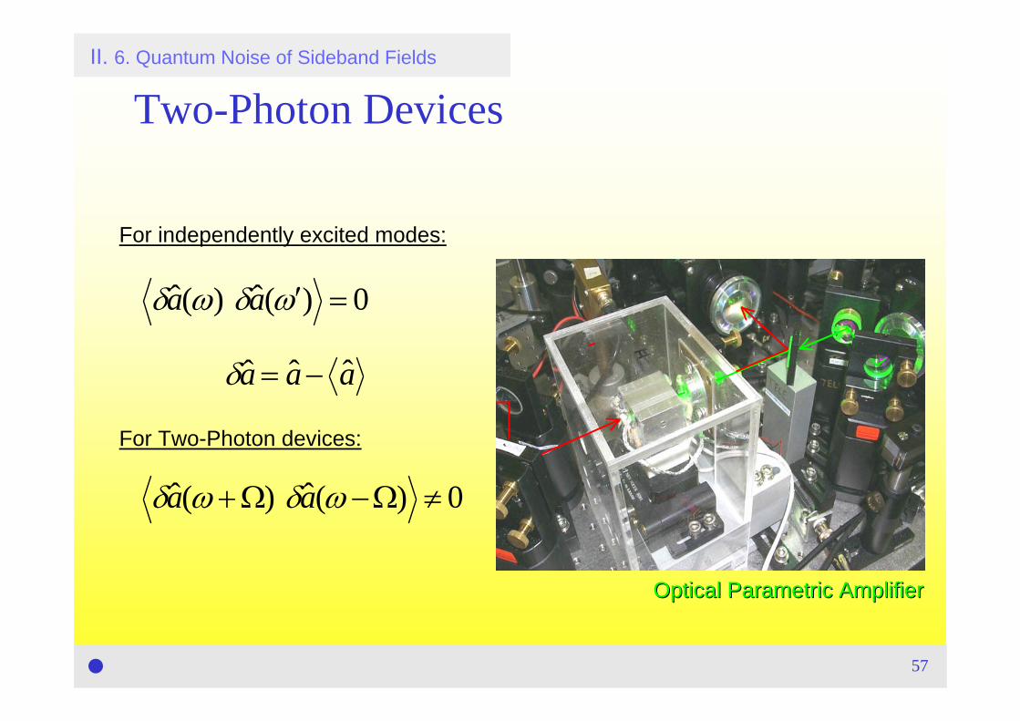
δˆ a (ω) δˆ a ( ′ ω ) = 0
δˆ a = ˆ a − ˆ a
δˆ a (ω + Ω) δˆ a (ω − Ω) ≠ 0
Two-Photon DevicesII. 6. Quantum Noise of Sideband Fields
For independently excited modes:
For Two-Photon devices:
Optical Parametric AmplifierOptical Parametric Amplifier
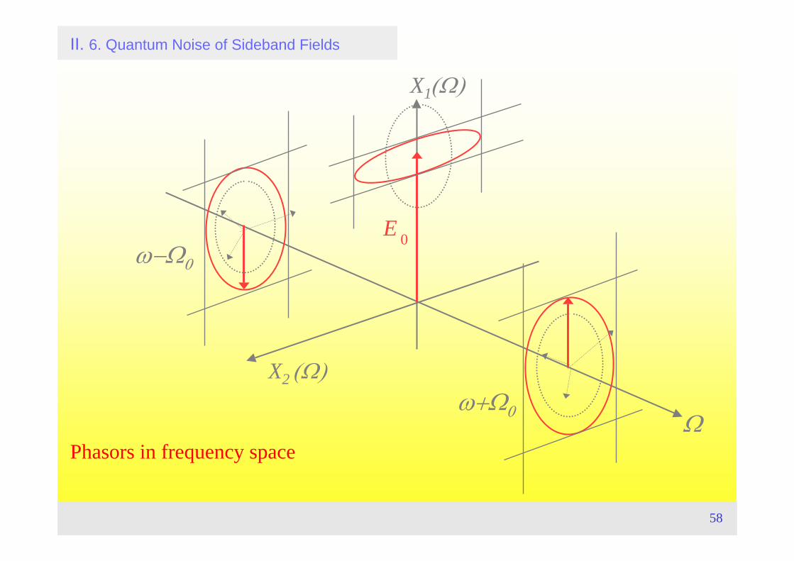
58
Phasors in frequency spaceΩ
X1(Ω)
E 0
ω+Ω0
ω−Ω0
X2 (Ω)
II. 6. Quantum Noise of Sideband Fields
59
II. Interferometer Quantum Noise: Basics and Tools 7. Quadrature Input-Output Relations
TopicsModular input-output-relations for optical devices:
- free propagation- beam splitters- cavities- interferometers
Literature• M. J. Collet and C. W. Gardiner, Phys. Rev. A 30, 1386 (1984),• Jan Harms, Diploma Thesis, Hannover University 2002,
Quantum Noise in the Laser-Interferometer Gravitational-Wave Detector GEO600
60
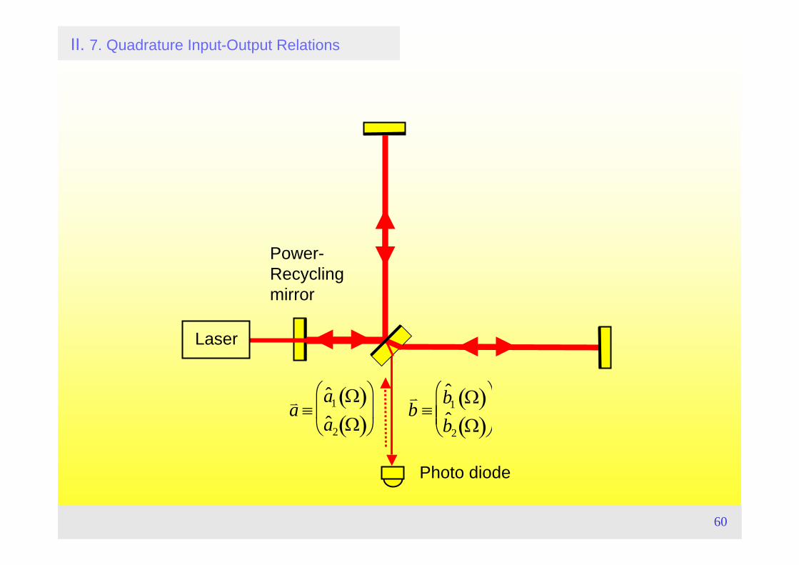
II. 7. Quadrature Input-Output Relations
Power-Recyclingmirror
Laser
Photo diode
v a ≡ˆ a 1 Ω( )ˆ a 2 Ω( )
⎛
⎝ ⎜
⎞
⎠ ⎟
v b ≡
ˆ b 1 Ω( )ˆ b 2 Ω( )
⎛
⎝ ⎜ ⎜
⎞
⎠ ⎟ ⎟
61
Quantum noise in phase quadrature
Quantum Noise of a Conventional MI
Standard quantum limit
(SQL)
Quantum noisewith increased laser
power (x100)
Shot noise
Radiation pressure noise
II. 4. Quantum Noise Spectral Densities
62
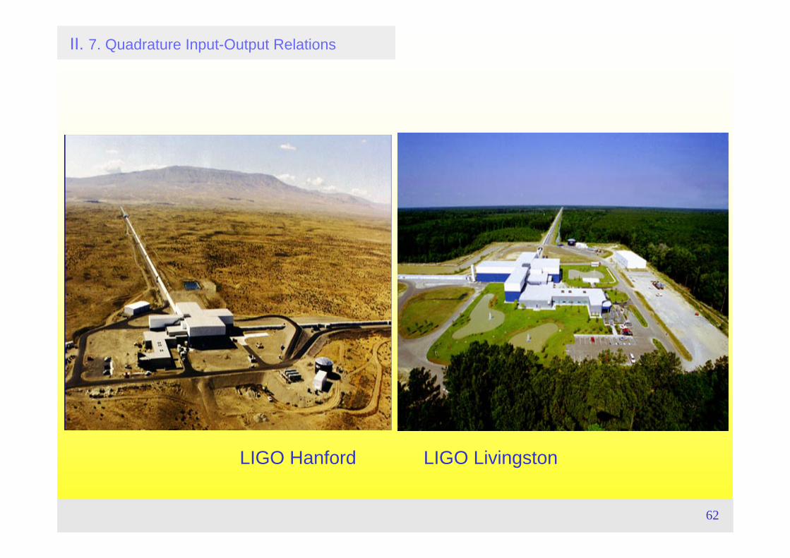
II. 7. Quadrature Input-Output Relations
LIGO Hanford LIGO Livingston
63
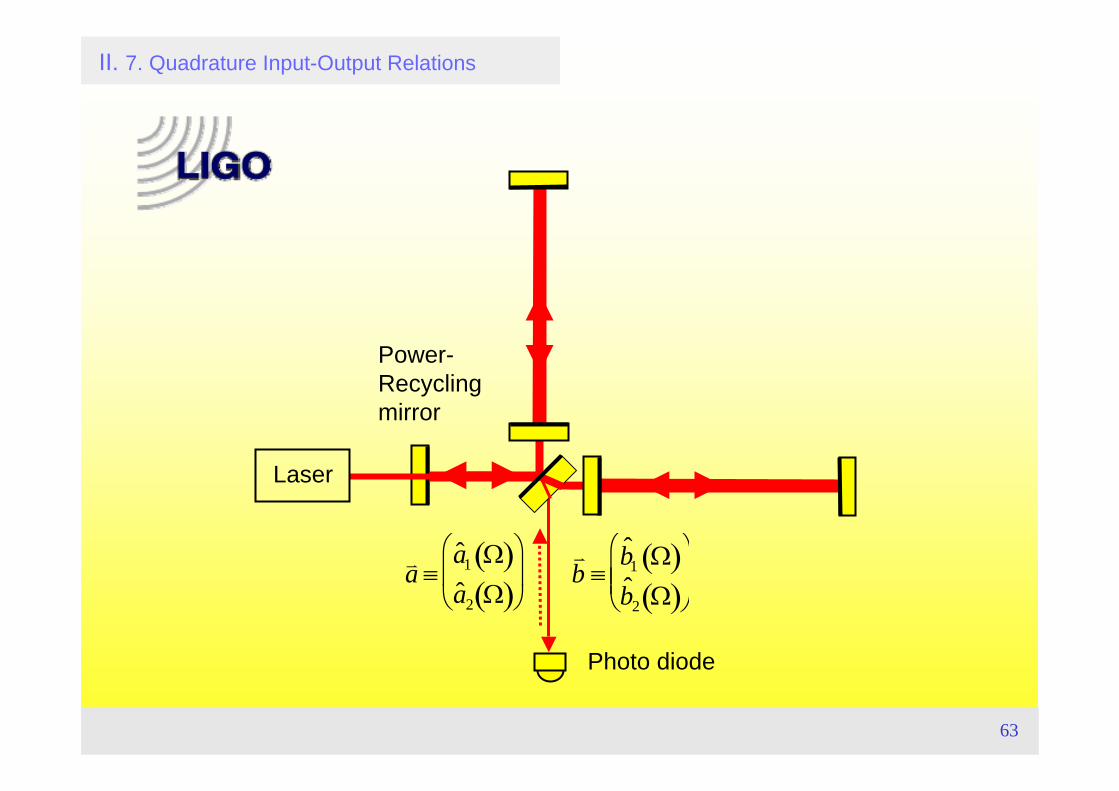
II. 7. Quadrature Input-Output Relations
Power-Recyclingmirror
Laser
Photo diode
v a ≡ˆ a 1 Ω( )ˆ a 2 Ω( )
⎛
⎝ ⎜
⎞
⎠ ⎟
v b ≡
ˆ b 1 Ω( )ˆ b 2 Ω( )
⎛
⎝ ⎜ ⎜
⎞
⎠ ⎟ ⎟
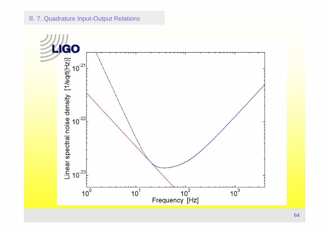
64
II. 7. Quadrature Input-Output Relations
65
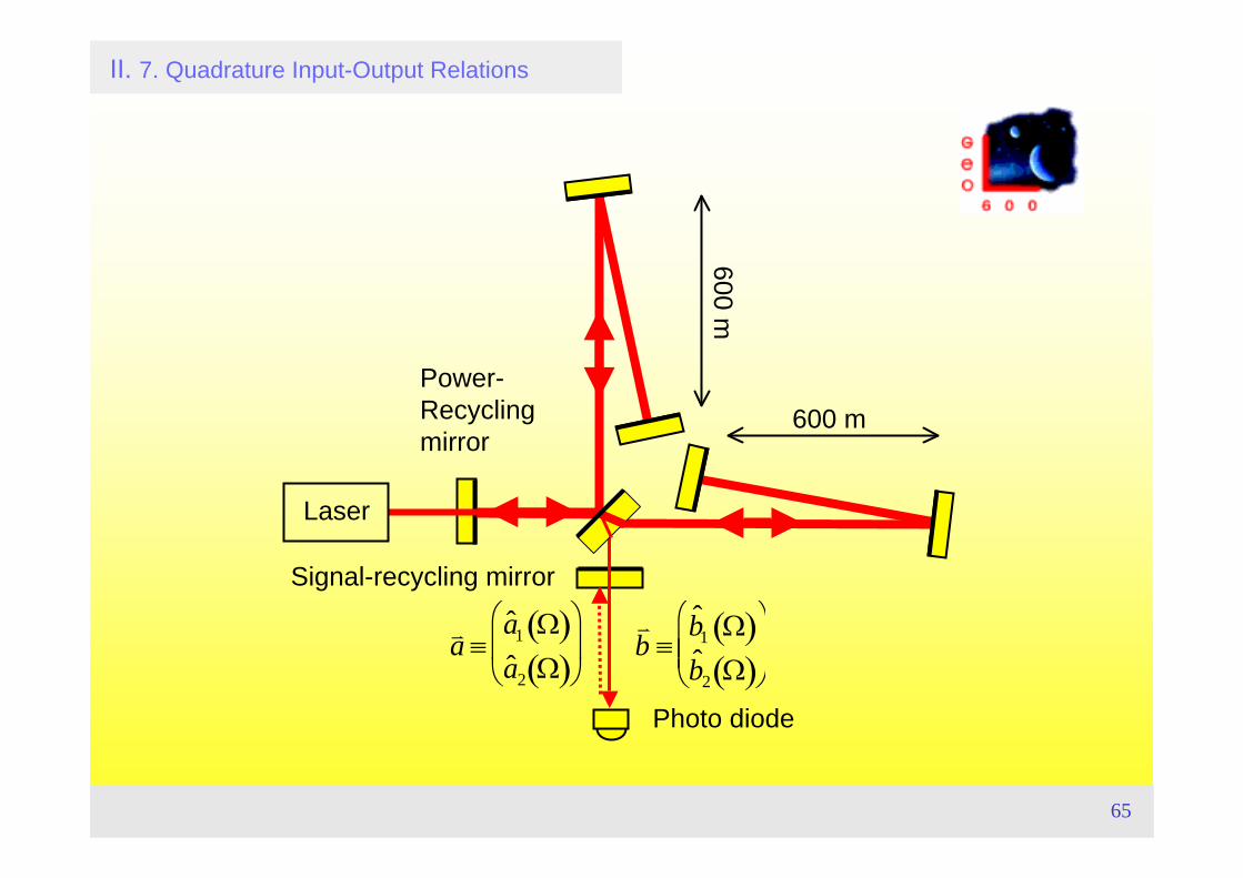
II. 7. Quadrature Input-Output Relations
Signal-recycling mirror
Power-Recyclingmirror
Laser
Photo diode
600 m
600 m
v a ≡ˆ a 1 Ω( )ˆ a 2 Ω( )
⎛
⎝ ⎜
⎞
⎠ ⎟
v b ≡
ˆ b 1 Ω( )ˆ b 2 Ω( )
⎛
⎝ ⎜ ⎜
⎞
⎠ ⎟ ⎟
66
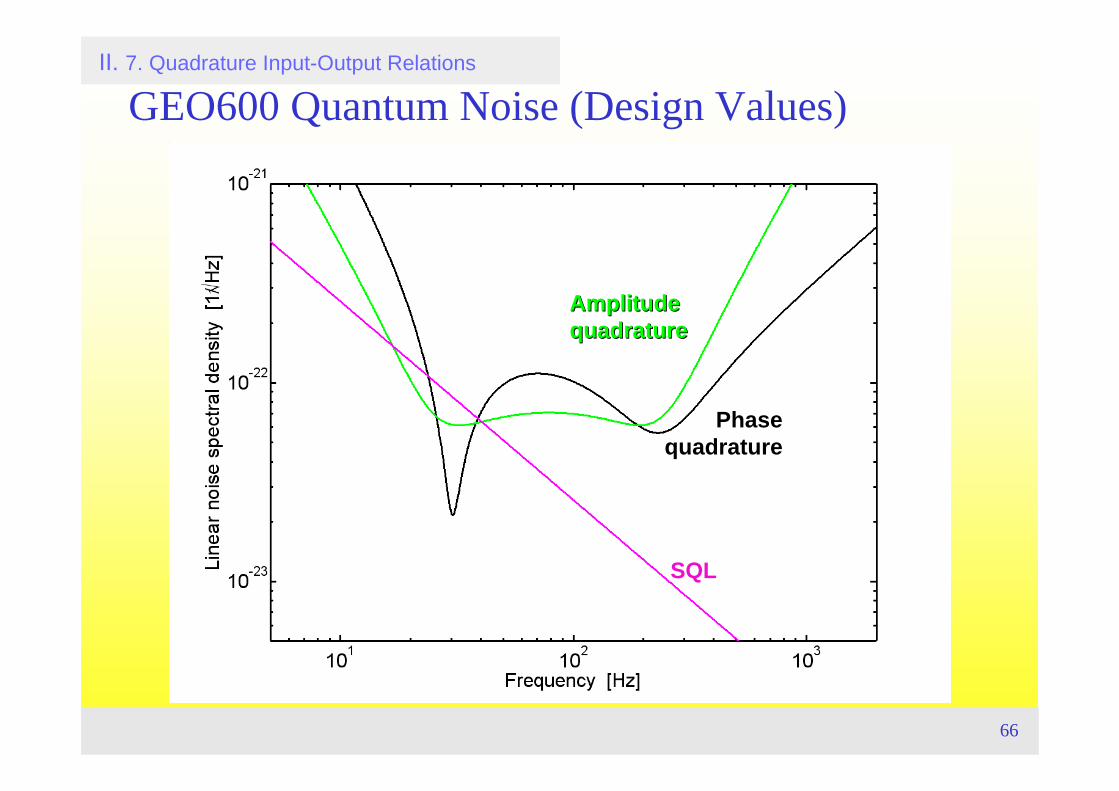
GEO600 Quantum Noise (Design Values)II. 7. Quadrature Input-Output Relations
Phasequadrature
AmplitudeAmplitudequadraturequadrature
SQL
67
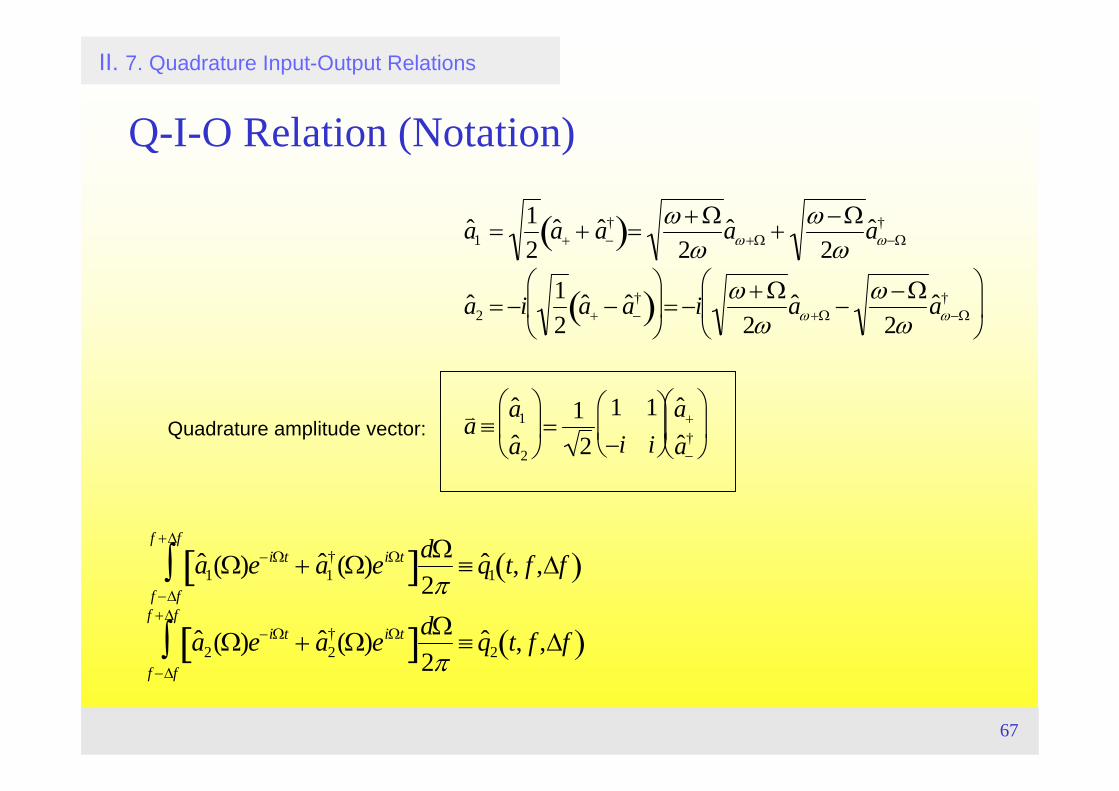
Q-I-O Relation (Notation)
II. 7. Quadrature Input-Output Relations
ˆ a 1(Ω)e−iΩt + ˆ a 1†(Ω)eiΩt[ ]dΩ
2πf −Δf
f +Δf
∫ ≡ ˆ q 1 t, f ,Δf( )
ˆ a 2(Ω)e−iΩt + ˆ a 2†(Ω)eiΩt[ ]dΩ
2πf −Δf
f +Δf
∫ ≡ ˆ q 2 t, f ,Δf( )
ˆ a 1 =12
ˆ a + + ˆ a −†( )=
ω + Ω2ω
ˆ a ω +Ω +ω − Ω
2ωˆ a ω−Ω
†
ˆ a 2 = −i 12
ˆ a + − ˆ a −†( )
⎛
⎝ ⎜
⎞
⎠ ⎟ = −i ω + Ω
2ωˆ a ω +Ω −
ω − Ω2ω
ˆ a ω−Ω†
⎛
⎝ ⎜
⎞
⎠ ⎟
v a ≡ˆ a 1ˆ a 2
⎛
⎝ ⎜
⎞
⎠ ⎟ =
12
1 1−i i
⎛
⎝ ⎜
⎞
⎠ ⎟
ˆ a +ˆ a −
†
⎛
⎝ ⎜
⎞
⎠ ⎟ Quadrature amplitude vector:
68
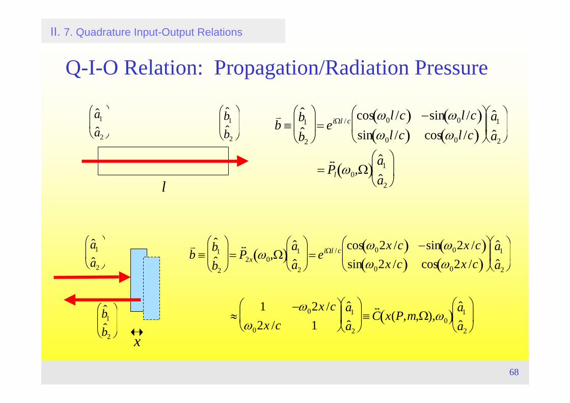
Q-I-O Relation: Propagation/Radiation Pressure
II. 7. Quadrature Input-Output Relations
v b ≡
ˆ b 1ˆ b 2
⎛
⎝ ⎜
⎞
⎠ ⎟ = eiΩl / c cos ω0l /c( ) −sin ω0l /c( )
sin ω0l /c( ) cos ω0l /c( )⎛
⎝ ⎜
⎞
⎠ ⎟
ˆ a 1ˆ a 2
⎛
⎝ ⎜
⎞
⎠ ⎟
=t P l ω0,Ω( )
ˆ a 1ˆ a 2
⎛
⎝ ⎜
⎞
⎠ ⎟
ˆ a 1ˆ a 2
⎛
⎝ ⎜
⎞
⎠ ⎟
ˆ b 1ˆ b 2
⎛
⎝ ⎜
⎞
⎠ ⎟
l
ˆ a 1ˆ a 2
⎛
⎝ ⎜
⎞
⎠ ⎟
ˆ b 1ˆ b 2
⎛
⎝ ⎜
⎞
⎠ ⎟
x
v b ≡
ˆ b 1ˆ b 2
⎛
⎝ ⎜
⎞
⎠ ⎟ =
t P 2x ω0,Ω( )
ˆ a 1ˆ a 2
⎛
⎝ ⎜
⎞
⎠ ⎟ = eiΩl / c cos ω02x /c( ) −sin ω02x /c( )
sin ω02x /c( ) cos ω02x /c( )⎛
⎝ ⎜
⎞
⎠ ⎟
ˆ a 1ˆ a 2
⎛
⎝ ⎜
⎞
⎠ ⎟
≈1 −ω02x /c
ω02x /c 1⎛
⎝ ⎜
⎞
⎠ ⎟
ˆ a 1ˆ a 2
⎛
⎝ ⎜
⎞
⎠ ⎟ ≡
t C x(P,m,Ω),ω0( )
ˆ a 1ˆ a 2
⎛
⎝ ⎜
⎞
⎠ ⎟
69
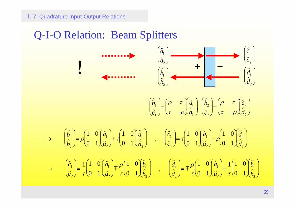
Q-I-O Relation: Beam Splitters
II. 7. Quadrature Input-Output Relations
ˆ b 1ˆ c 1
⎛
⎝ ⎜
⎞
⎠ ⎟ =
ρ ττ −ρ
⎛
⎝ ⎜
⎞
⎠ ⎟
ˆ a 1ˆ d 1
⎛
⎝ ⎜
⎞
⎠ ⎟ ,
ˆ b 2ˆ c 2
⎛
⎝ ⎜
⎞
⎠ ⎟ =
ρ ττ −ρ
⎛
⎝ ⎜
⎞
⎠ ⎟
ˆ a 2ˆ d 2
⎛
⎝ ⎜
⎞
⎠ ⎟
⇒ˆ b 1ˆ b 2
⎛
⎝ ⎜
⎞
⎠ ⎟ = ρ
1 00 1
⎛
⎝ ⎜
⎞
⎠ ⎟
ˆ a 1ˆ a 2
⎛
⎝ ⎜
⎞
⎠ ⎟ + τ
1 00 1
⎛
⎝ ⎜
⎞
⎠ ⎟
ˆ d 1ˆ d 2
⎛
⎝ ⎜
⎞
⎠ ⎟ ,
ˆ c 1ˆ c 2
⎛
⎝ ⎜
⎞
⎠ ⎟ = τ
1 00 1
⎛
⎝ ⎜
⎞
⎠ ⎟
ˆ a 1ˆ a 2
⎛
⎝ ⎜
⎞
⎠ ⎟ − ρ
1 00 1
⎛
⎝ ⎜
⎞
⎠ ⎟
ˆ d 1ˆ d 2
⎛
⎝ ⎜
⎞
⎠ ⎟
ˆ a 1ˆ a 2
⎛
⎝ ⎜
⎞
⎠ ⎟
ˆ b 1ˆ b 2
⎛
⎝ ⎜
⎞
⎠ ⎟
+ −
ˆ c 1ˆ c 2
⎛
⎝ ⎜
⎞
⎠ ⎟
ˆ d 1ˆ d 2
⎛
⎝ ⎜
⎞
⎠ ⎟
⇒ˆ c 1ˆ c 2
⎛
⎝ ⎜
⎞
⎠ ⎟ =
1τ
1 00 1
⎛
⎝ ⎜
⎞
⎠ ⎟
ˆ a 1ˆ a 2
⎛
⎝ ⎜
⎞
⎠ ⎟ m
ρτ
1 00 1
⎛
⎝ ⎜
⎞
⎠ ⎟
ˆ b 1ˆ b 2
⎛
⎝ ⎜
⎞
⎠ ⎟ ,
ˆ d 1ˆ d 2
⎛
⎝ ⎜
⎞
⎠ ⎟ = m
ρτ
1 00 1
⎛
⎝ ⎜
⎞
⎠ ⎟
ˆ a 1ˆ a 2
⎛
⎝ ⎜
⎞
⎠ ⎟ +
1τ
1 00 1
⎛
⎝ ⎜
⎞
⎠ ⎟
ˆ b 1ˆ b 2
⎛
⎝ ⎜
⎞
⎠ ⎟
!
70
III. Schemes for Nonclassical Interferometers 8. Simple MI with Squeezed Light Input
TopicsQuadrature transfer function of a simple Michelson interferometer,
normalized to ist noise spectral densityA quantum noise MATLAB code Squeezed light input for a simple Michelson interferometerBeating the Standard Quantum Limit
Literature• H. J. Kimble, Y. Levin, A. B. Matsko, K. S. Thorne, and S. P. Vyatchanin,
Phys. Rev. D 65, 022002 (2001), Conversion of conventional gravitational-wave interferometers into quantum nondemolition interferometers by modifying their input and/or output optics
71
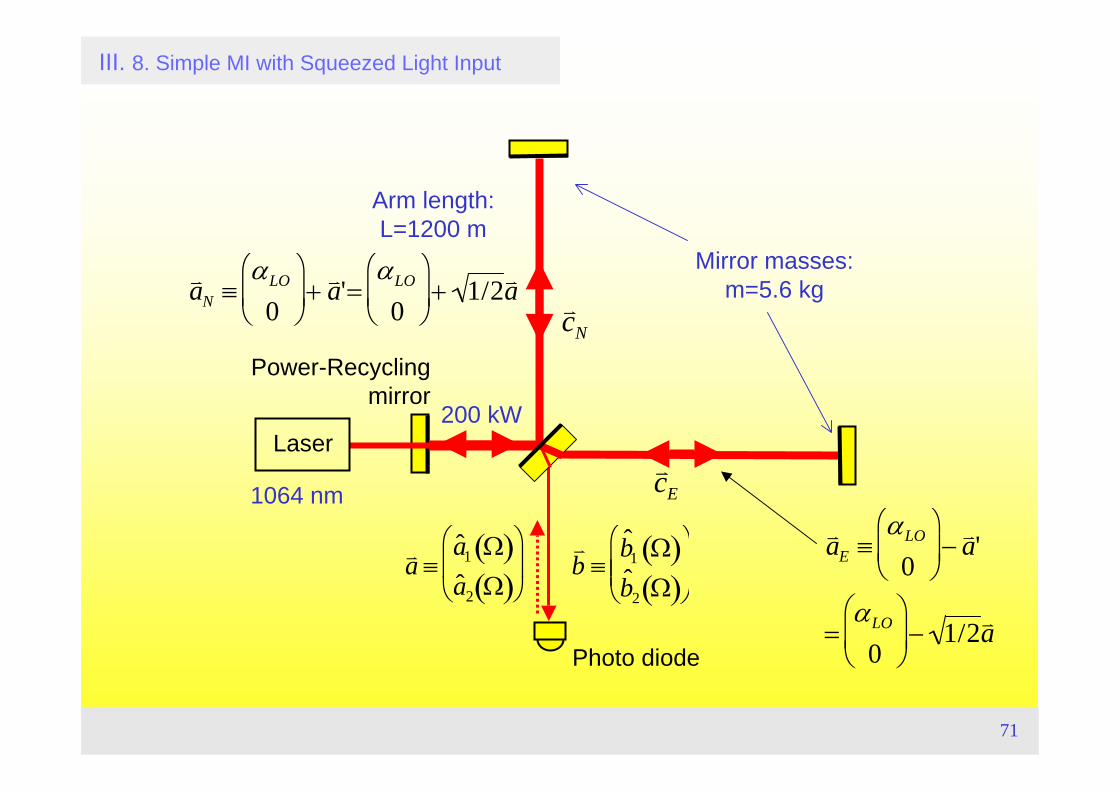
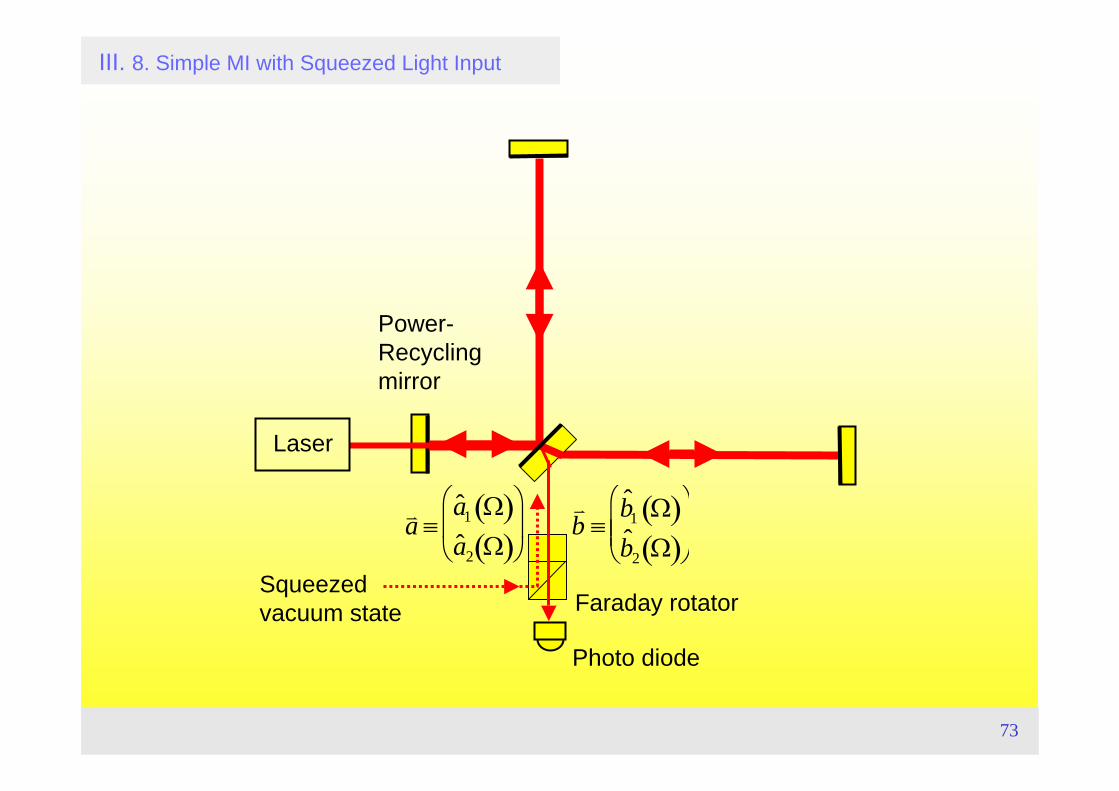
III. 8. Simple MI with Squeezed Light Input
Power-Recyclingmirror
Laser
Photo diode
1064 nm
Mirror masses:m=5.6 kg
Arm length:L=1200 m
200 kW
v a N ≡αLO
0⎛
⎝ ⎜
⎞
⎠ ⎟ +
v a '=αLO
0⎛
⎝ ⎜
⎞
⎠ ⎟ + 1/2v a
Ecv
Ncv
v a ≡ˆ a 1 Ω( )ˆ a 2 Ω( )
⎛
⎝ ⎜
⎞
⎠ ⎟
v b ≡
ˆ b 1 Ω( )ˆ b 2 Ω( )
⎛
⎝ ⎜ ⎜
⎞
⎠ ⎟ ⎟
v a E ≡αLO
0⎛
⎝ ⎜
⎞
⎠ ⎟ −
v a '
=αLO
0⎛
⎝ ⎜
⎞
⎠ ⎟ − 1/2v a
72
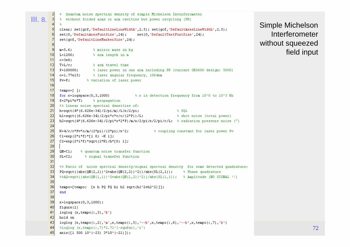
III. 8. Simple MI with Squeezed Light InputSimple Michelson
Interferometer without squeezed
field input
73
III. 8. Simple MI with Squeezed Light Input
Power-Recyclingmirror
Laser
Photo diode
Squeezed vacuum state Faraday rotator
v a ≡ˆ a 1 Ω( )ˆ a 2 Ω( )
⎛
⎝ ⎜
⎞
⎠ ⎟
v b ≡
ˆ b 1 Ω( )ˆ b 2 Ω( )
⎛
⎝ ⎜ ⎜
⎞
⎠ ⎟ ⎟
74
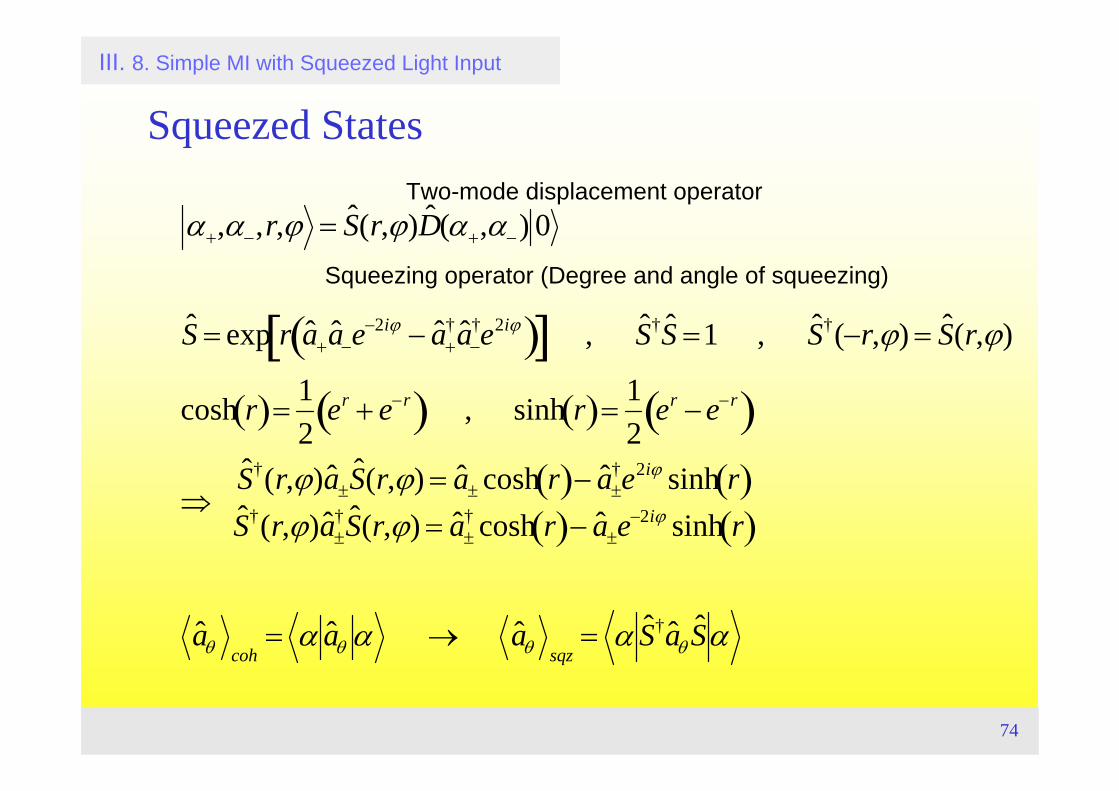
III. 8. Simple MI with Squeezed Light Input
Squeezed States
α+,α−,r,ϕ = ˆ S (r,ϕ) ˆ D (α+,α−) 0
ˆ S = exp r ˆ a + ˆ a −e−2iϕ − ˆ a +
† ˆ a −†e2iϕ( )[ ] , ˆ S † ˆ S =1 , ˆ S †(−r,ϕ) = ˆ S (r,ϕ)
cosh r( )=12
er + e−r( ) , sinh r( )=12
er −e−r( )
⇒ˆ S †(r,ϕ) ˆ a ± ˆ S (r,ϕ) = ˆ a ± cosh r( )− ˆ a ±
†e2iϕ sinh r( )ˆ S †(r,ϕ) ˆ a ±
† ˆ S (r,ϕ) = ˆ a ±† cosh r( )− ˆ a ±e
−2iϕ sinh r( )
ˆ a θ coh= α ˆ a θ α → ˆ a θ sqz
= α ˆ S † ˆ a θ ˆ S α
Squeezing operator (Degree and angle of squeezing)
Two-mode displacement operator
75
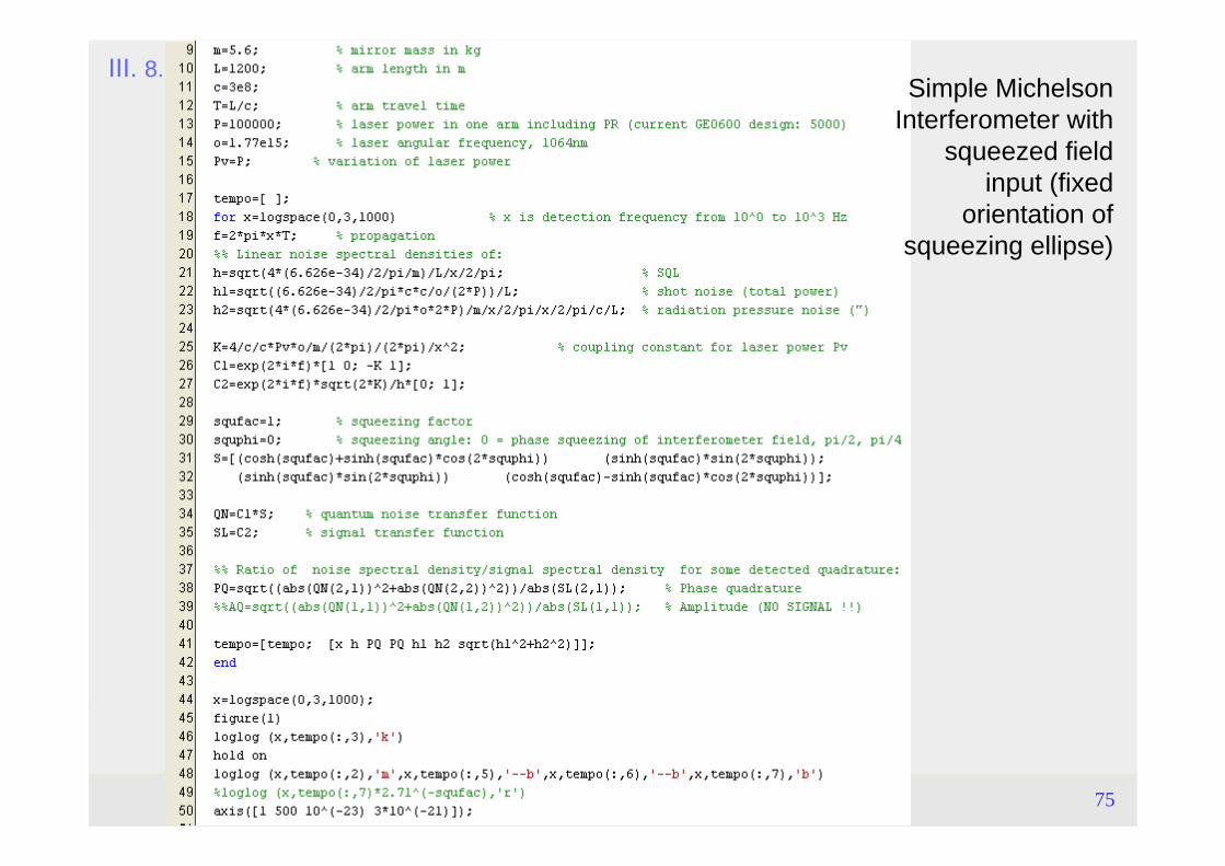
III. 8. Simple MI with Squeezed Light InputSimple Michelson
Interferometer with squeezed field
input (fixed orientation of
squeezing ellipse)
76
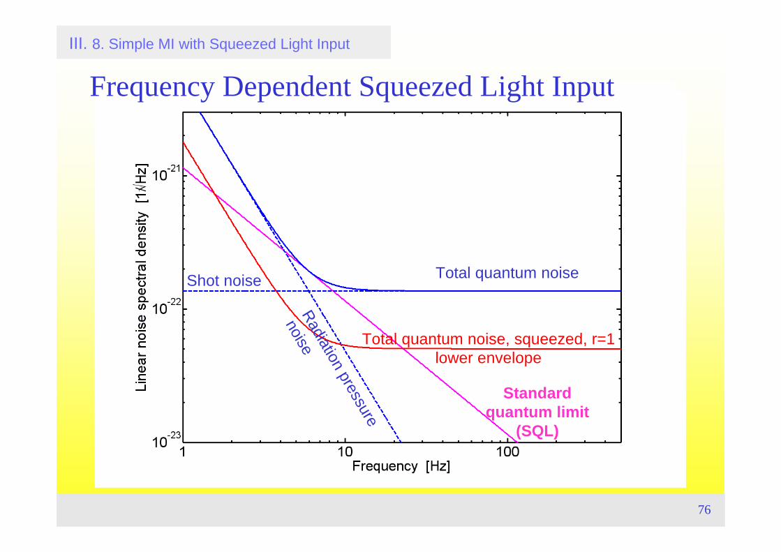
III. 8. Simple MI with Squeezed Light Input
Total quantum noise, squeezed, r=1lower envelope
Standard quantum limit
(SQL)
Shot noise
Radiation pressure
noise
Total quantum noise
Frequency Dependent Squeezed Light Input
77
III. Schemes for Nonclassical Interferometers 9. Variational Output
TopicsVariational output (frequency dependent homodyne detection)QND interferometry without injected squeezed states„Self-squeezing“: Ponderomotively squeezed lightRadiation pressure Kerr nonlinearityProposal for an experimental realization„Squeezed input – variational output“
Literature• H. J. Kimble, Y. Levin, A. B. Matsko, K. S. Thorne, and S. P. Vyatchanin,
Phys. Rev. D 65, 022002 (2001), Conversion of conventional gravitational-wave interferometers into quantum nondemolition interferometers by modifying their input and/or output optics
• R. Loudon, Phys. Rev. Lett., 47 , 815 (1981)Quantum Limit on the Michelson Interferometer used for Gravitational-Wave Detection
78
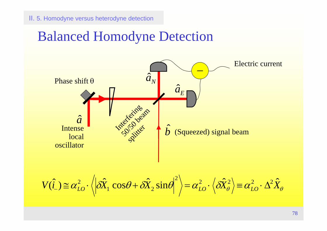
(Squeezed) signal beamIntense local
oscillator
Phase shift θ
Electric current
V(ˆ i −) ≅ αLO2 ⋅ δ ˆ X 1 cosθ +δ ˆ X 2 sinθ
2= αLO
2 ⋅ δ ˆ X θ2 ≡ αLO
2 ⋅ Δ2 ˆ X θ
Balanced Homodyne Detection
Interf
ering
50/50
beam
splitte
r
II. 5. Homodyne versus heterodyne detection
ab
NaEa
79
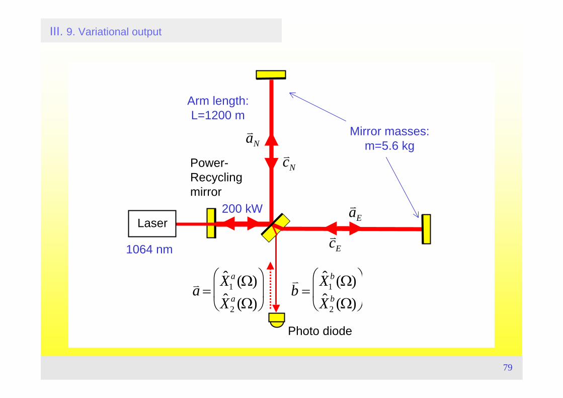
v a =ˆ X 1
a (Ω)ˆ X 2
a (Ω)
⎛
⎝ ⎜
⎞
⎠ ⎟
v b =
ˆ X 1b(Ω)
ˆ X 2b(Ω)
⎛
⎝ ⎜
⎞
⎠ ⎟
III. 9. Variational output
Power-Recyclingmirror
Laser
Photo diode
1064 nm
Mirror masses:m=5.6 kg
Arm length:L=1200 m
200 kW
Nav
Eav
Ecv
Ncv
80
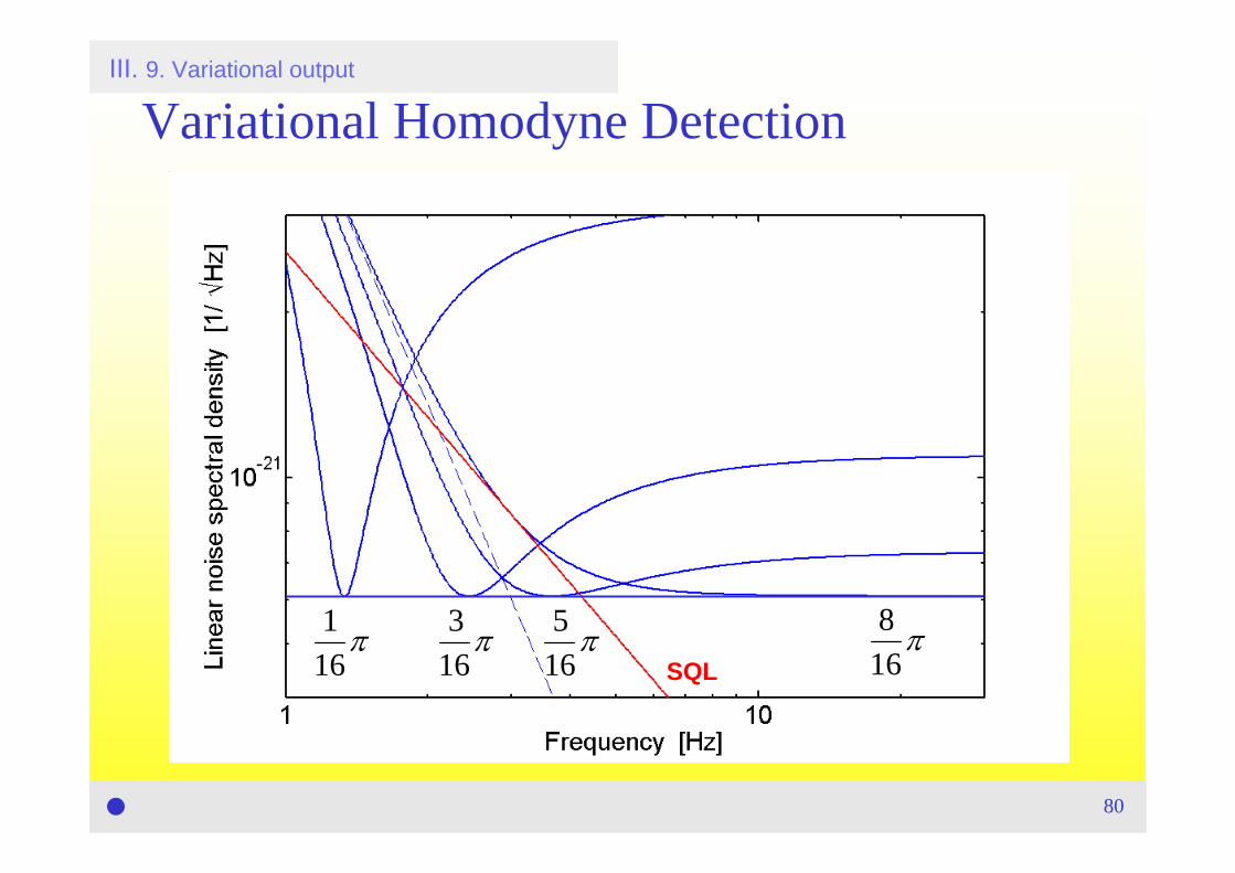
Variational Homodyne Detection
SQL
116
π 316
π 516
π8
16π
III. 9. Variational output
81
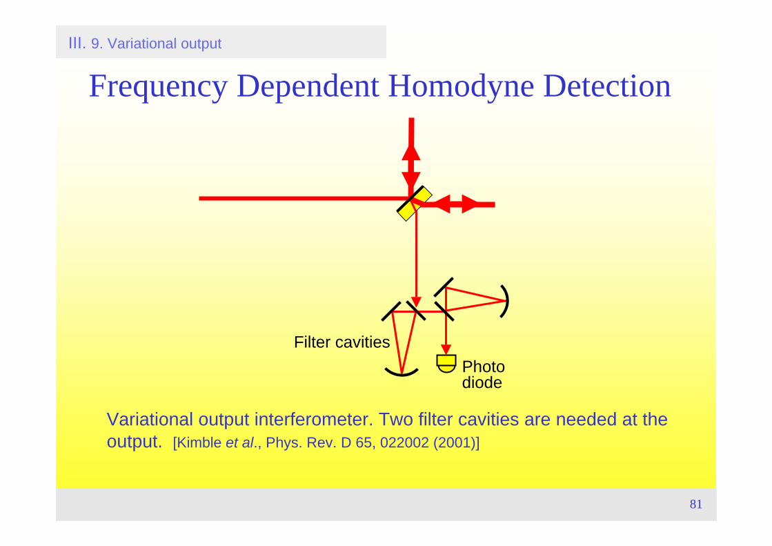
Photodiode
Filter cavities
Frequency Dependent Homodyne Detection
Variational output interferometer. Two filter cavities are needed at the output. [Kimble et al., Phys. Rev. D 65, 022002 (2001)]
III. 9. Variational output
82
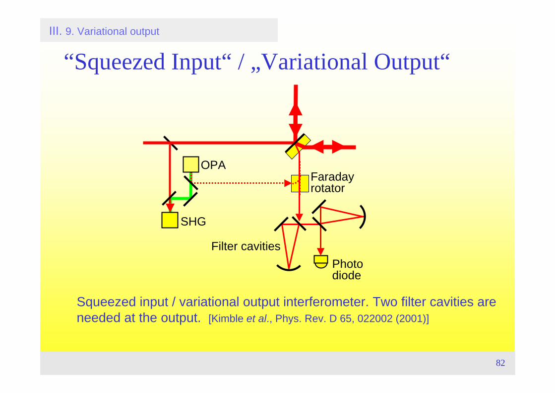
Faraday rotator
SHG
OPA
Photodiode
Filter cavities
“Squeezed Input“ / „Variational Output“
Squeezed input / variational output interferometer. Two filter cavities are needed at the output. [Kimble et al., Phys. Rev. D 65, 022002 (2001)]
III. 9. Variational output
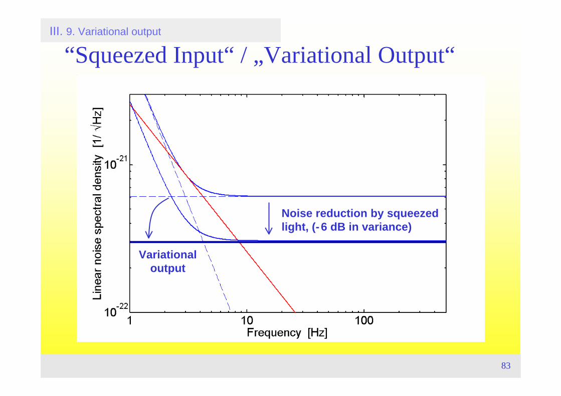
83
Noise reduction by squeezed light, (-6 dB in variance)
“Squeezed Input“ / „Variational Output“III. 9. Variational output
Variationaloutput
84
III. Schemes for Nonclassical Interferometers 10. The Optical Spring Interferometer
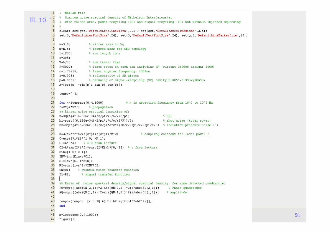
Topics(Detuned) signal recycling: GEO600A quantum noise MATLAB code
for GEO600, a signal recycled optical spring interferometerBeating the SQL by the optical spring effect
Literature• A. Buonanno and Y. Chen, Class. Quantum Gravity 18, L95 (2001),
Optical noise correlations and beating the standard quantum limit in advanced gravitational-wave detectors.
• B. S. Sheard, M. B. Gray, C. M. Mow-Lowry, D. E. McClelland, and S. E. Whitcomb, Phys. Rev. A 69, R 051801 (2004),Observation and characterization of an optical spring.
85
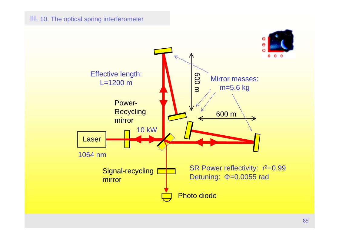
III. 10. The optical spring interferometer
Signal-recyclingmirror
Power-Recyclingmirror
Laser
Photo diode
600 m
600 m
1064 nm
Mirror masses:m=5.6 kg
Effective length:L=1200 m
SR Power reflectivity: r2=0.99Detuning: Φ=0.0055 rad
10 kW
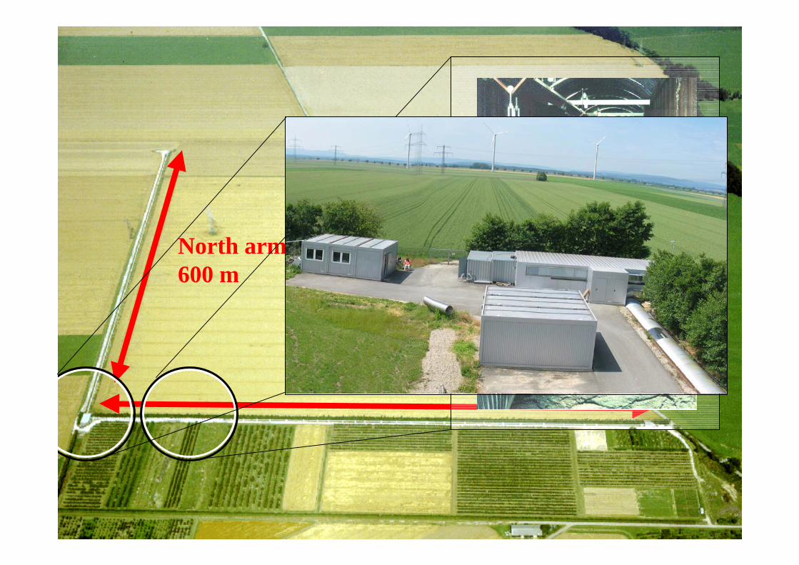
II. 9. The optical spring interferometer
East arm 600 m
North arm 600 m
600 m vacuum tube
87
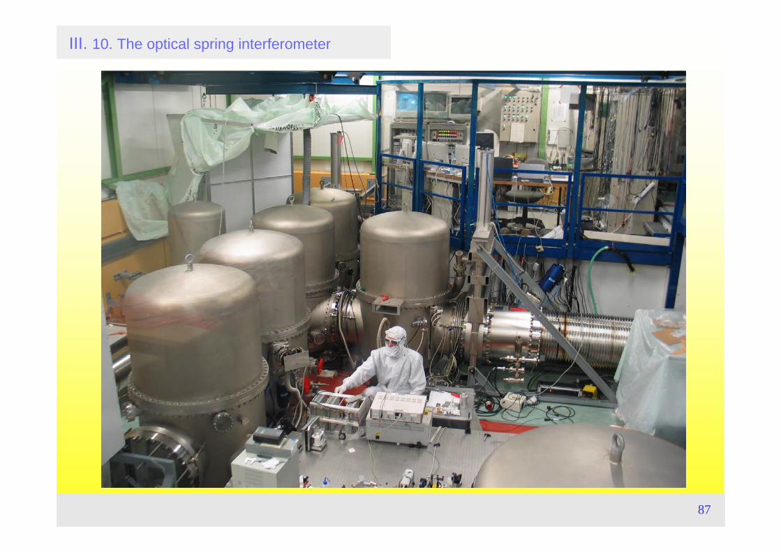
III. 10. The optical spring interferometer
88
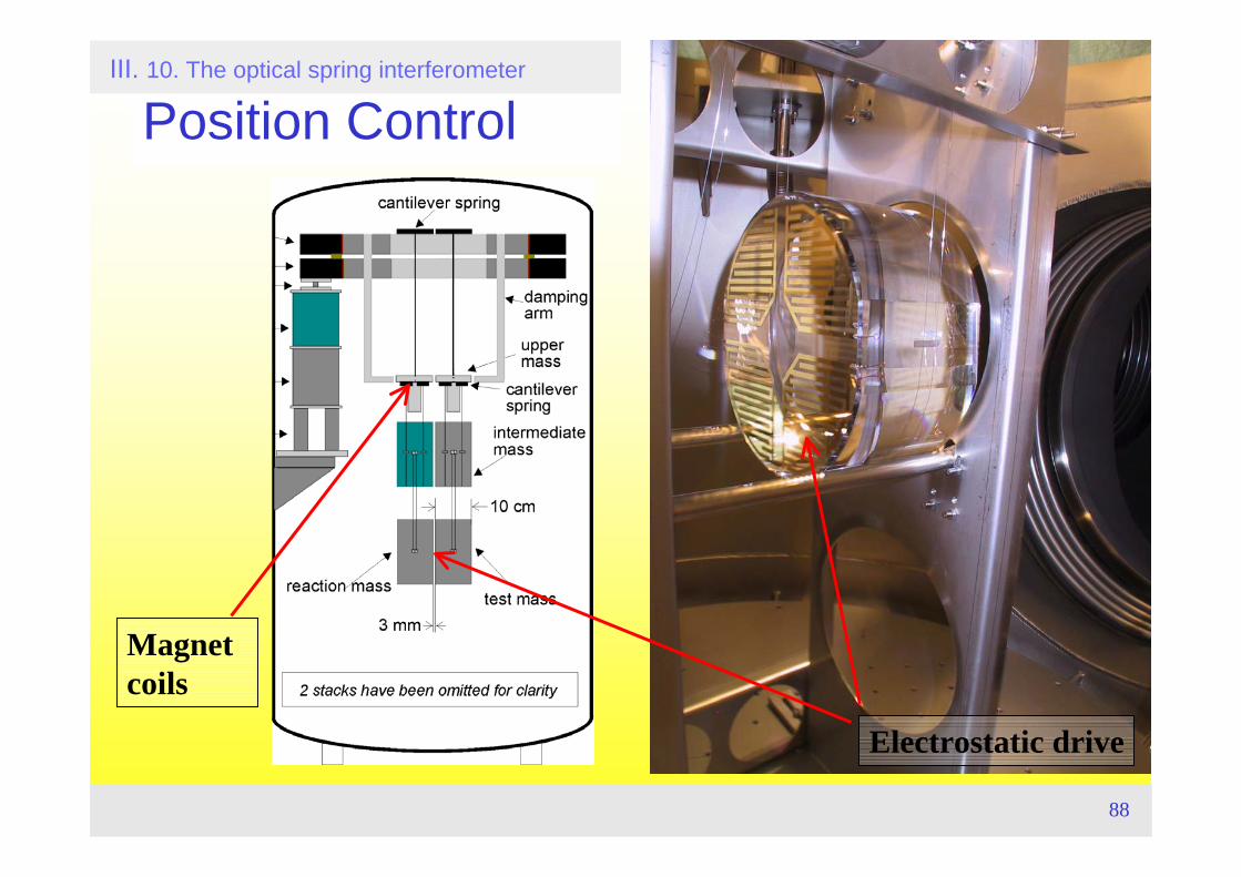
Position Control
Magnetcoils
Electrostatic drive
III. 10. The optical spring interferometer
89
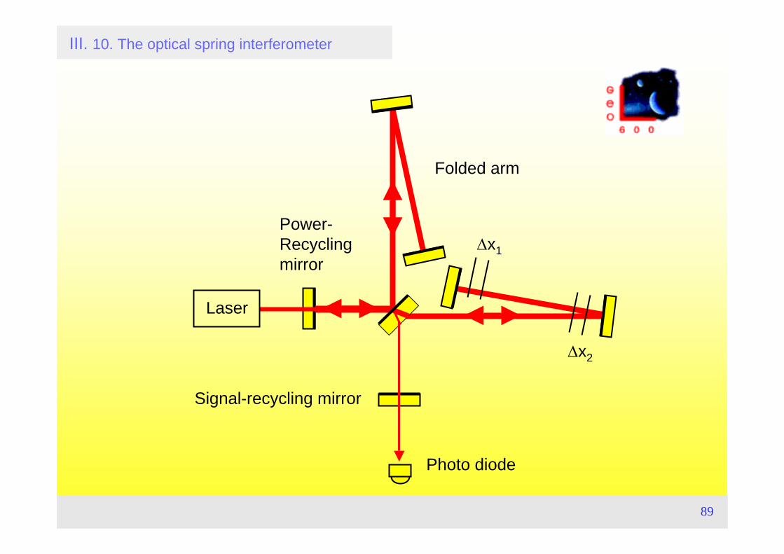
III. 10. The optical spring interferometer
Power-Recyclingmirror
Laser
Photo diode
Folded arm
Δx1
Δx2
Signal-recycling mirror
90
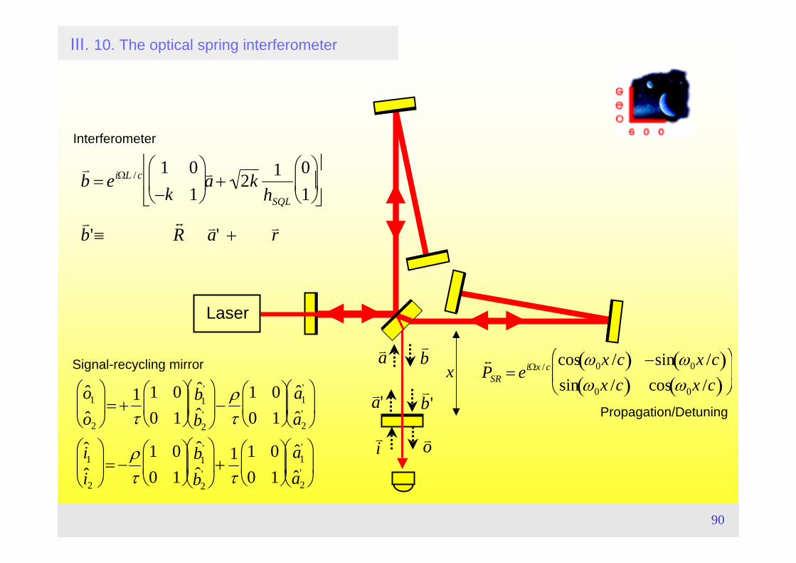
III. 10. The optical spring interferometer
Laser
v a
v b
v o
v i
v b = eiΩL / c 1 0
−k 1⎛
⎝ ⎜
⎞
⎠ ⎟ v a + 2k 1
hSQL
01
⎛
⎝ ⎜
⎞
⎠ ⎟
⎡
⎣ ⎢
⎤
⎦ ⎥
v b '≡
t R v a ' + v r
t P SR = eiΩx /c cos ω0x /c( ) −sin ω0x /c( )
sin ω0x /c( ) cos ω0x /c( )⎛
⎝ ⎜
⎞
⎠ ⎟
ˆ o 1ˆ o 2
⎛
⎝ ⎜
⎞
⎠ ⎟ = +
1τ
1 00 1
⎛
⎝ ⎜
⎞
⎠ ⎟
ˆ b 1'
ˆ b 2'
⎛
⎝ ⎜
⎞
⎠ ⎟ −
ρτ
1 00 1
⎛
⎝ ⎜
⎞
⎠ ⎟
ˆ a 1'
ˆ a 2'
⎛
⎝ ⎜
⎞
⎠ ⎟
ˆ i 1ˆ i 2
⎛
⎝ ⎜
⎞
⎠ ⎟ = −
ρτ
1 00 1
⎛
⎝ ⎜
⎞
⎠ ⎟
ˆ b 1'
ˆ b 2'
⎛
⎝ ⎜
⎞
⎠ ⎟ +
1τ
1 00 1
⎛
⎝ ⎜
⎞
⎠ ⎟
ˆ a 1'
ˆ a 2'
⎛
⎝ ⎜
⎞
⎠ ⎟
v a '
v b '
Interferometer
Signal-recycling mirror
Propagation/Detuning
x
91
III. 10. The optical spring interferometer

92
GEO600 Quantum Noise (Design Values)III. 10. The optical spring interferometer
Phasequadrature
AmplitudeAmplitudequadraturequadrature
(Without signal recycling)
SQL
93
III. Schemes for Nonclassical Interferometers 11. A Squeezed Light Upgraded GEO600 Detector?
TopicsOptical Spring Interferometer with
- squeezed input- variational output
Other noise sources than quantum in GEO600: Thermal, seismic noiseTable-top experimentsProposal for a squeezed light upgraded GEO600 detector
Literature• J. Harms, Y. Chen, S. Chelkowski, A. Franzen, H. Vahlbruch, K. Danzmann,
and R. Schnabel, Phys. Rev. D 68, 042001 (2003),Squeezed-input, optical-spring, signal-recycled gravitational-wave detectors.
• R. Schnabel, J. Harms, K. Strain, and K. Danzmann, Class. Quantum Grav. 21, S1045 (2003),Squeezed light for the interferometric detection of high-frequency gravitational waves.
94
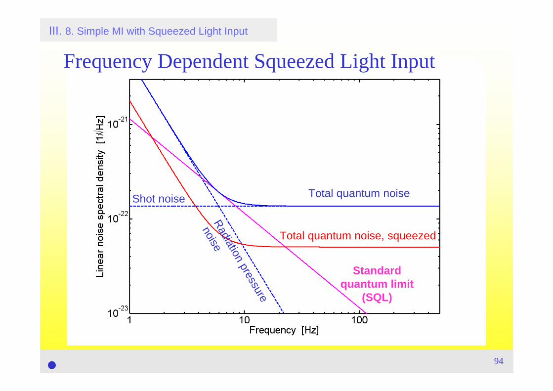
III. 8. Simple MI with Squeezed Light Input
Total quantum noise, squeezed
Standard quantum limit
(SQL)
Shot noise
Radiation pressure
noise
Total quantum noise
Frequency Dependent Squeezed Light Input
95
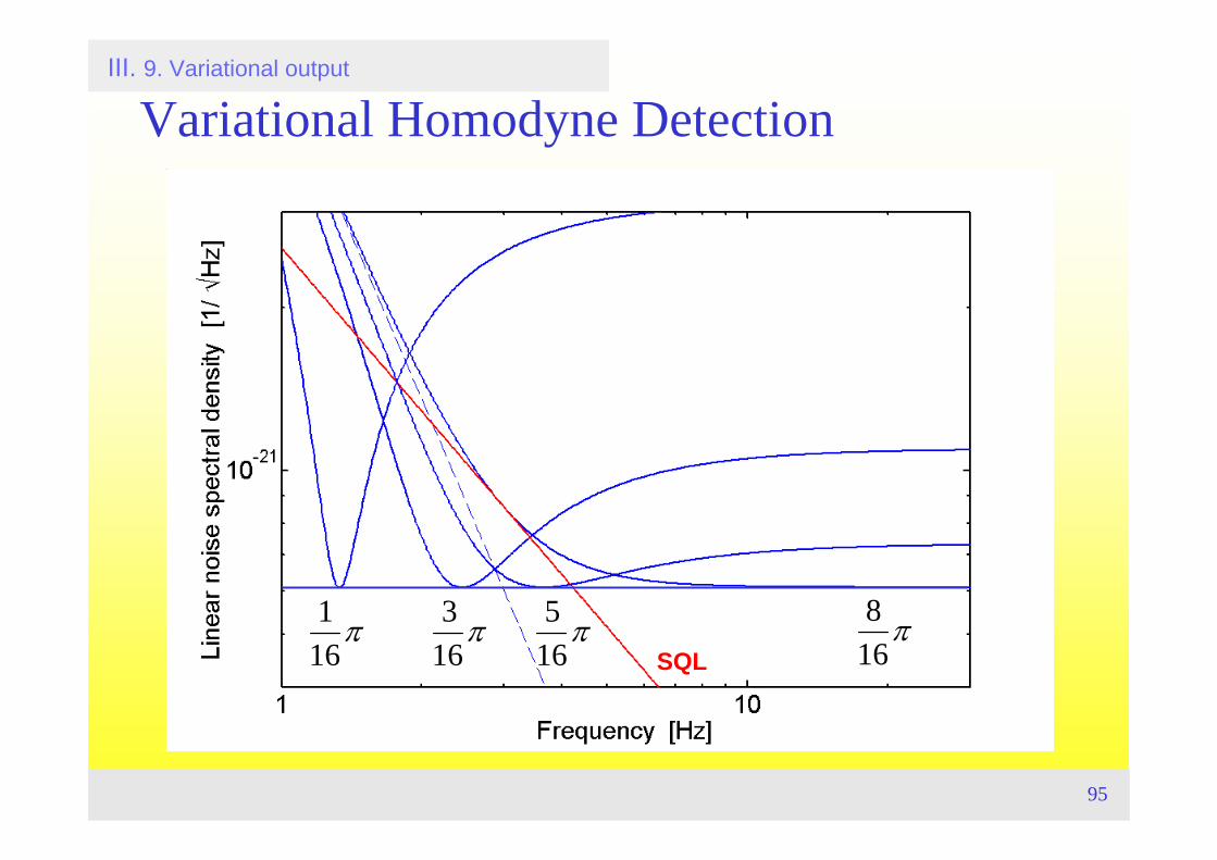
Variational Homodyne Detection
SQL
116
π 316
π 516
π8
16π
III. 9. Variational output

96
Noise reduction by squeezed light, (-6 dB in variance)
“Squeezed Input“ / „Variational Output“III. 9. Variational output
Variationaloutput
97
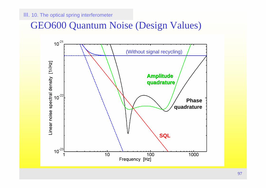
GEO600 Quantum Noise (Design Values)III. 10. The optical spring interferometer
Phasequadrature
AmplitudeAmplitudequadraturequadrature
(Without signal recycling)
SQL

98
GEO600 Quantum Noise (Design Values)III. 10. The optical spring interferometer
Phasequadrature
AmplitudeAmplitudequadraturequadrature
(Without signal recycling)
SQL
[J. Harms et al., PRD (2003)]
-6 dB
99
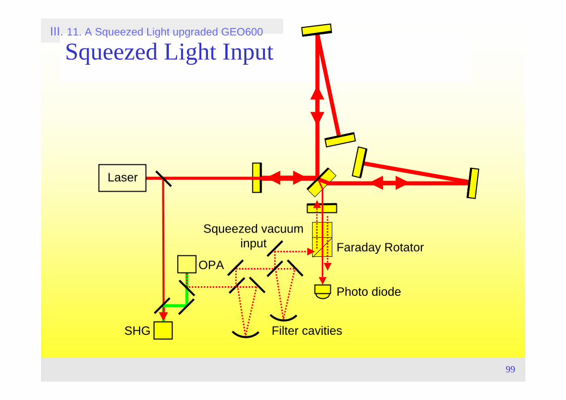
Squeezed Light Input
Laser
Faraday Rotator
Photo diode
SHG
OPA
Filter cavities
Squeezed vacuuminput
III. 11. A Squeezed Light upgraded GEO600
100
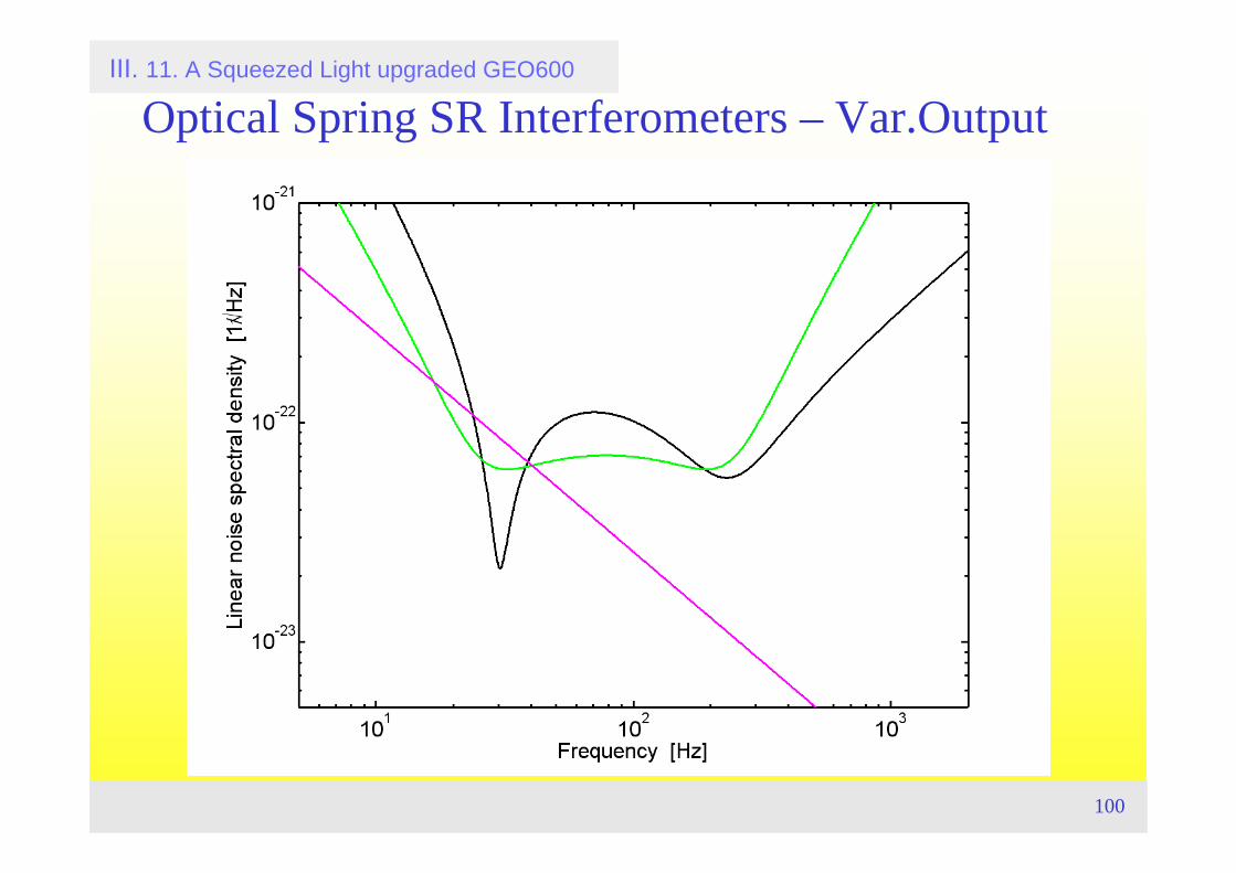
Optical Spring SR Interferometers – Var.OutputIII. 11. A Squeezed Light upgraded GEO600
101
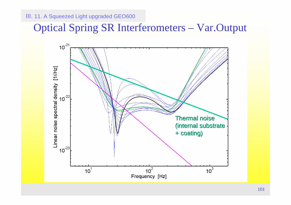
Optical Spring SR Interferometers – Var.OutputIII. 11. A Squeezed Light upgraded GEO600
Thermal noise Thermal noise ((internal internal substrate substrate + + coatingcoating))
102
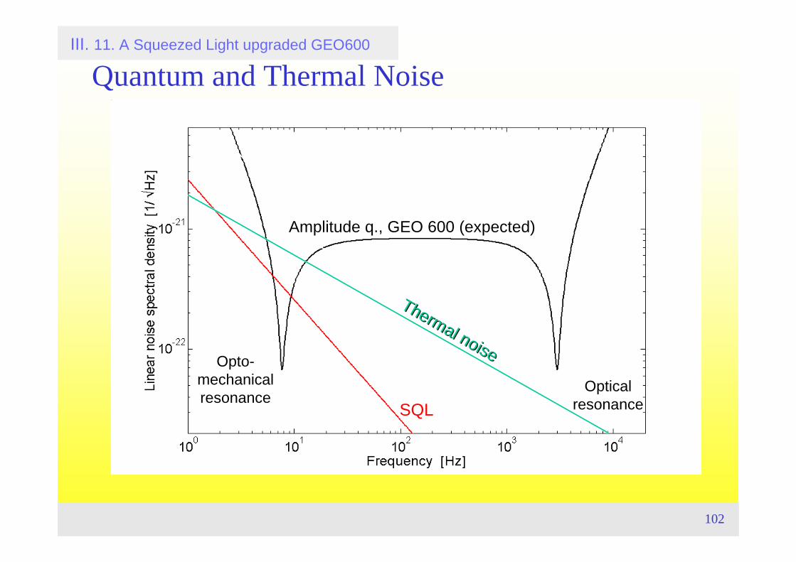
Thermal noise
Thermal noise
SQL
Quantum and Thermal NoiseIII. 11. A Squeezed Light upgraded GEO600
Amplitude q., GEO 600 (expected)
Opto-mechanical resonance
Optical resonance
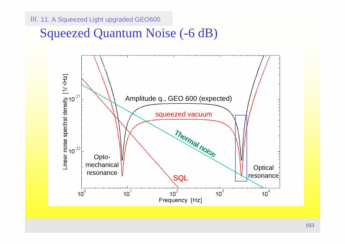
103
SQL
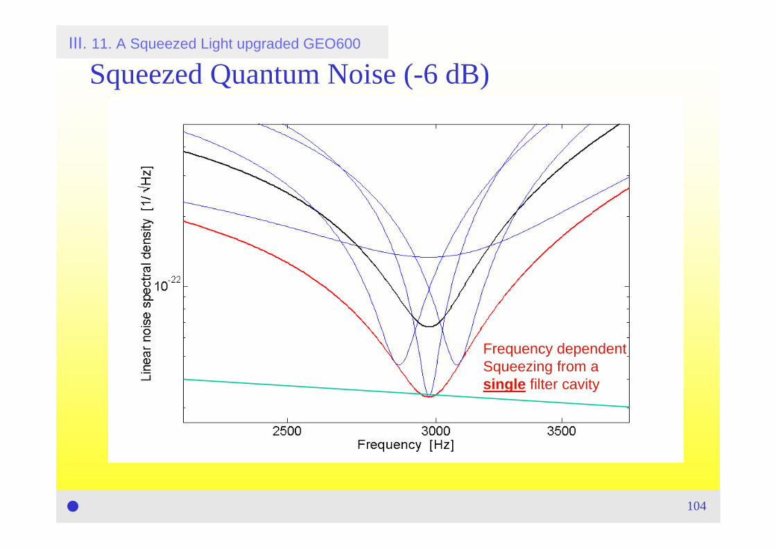
Squeezed Quantum Noise (-6 dB)
Thermal noise
Thermal noise
III. 11. A Squeezed Light upgraded GEO600
SQL
Amplitude q., GEO 600 (expected)
Opto-mechanical resonance
Optical resonance
squeezed vacuum
104
Phase squeezing
Squeezing at 45°
Phase squeezing
Amplitude squeezing
Phase squeezing
Squeezing at 45° Squeezing at -45°
Amplitude squeezing
Phase squeezing
Squeezing at 45° Frequency dependent Squeezing from a single filter cavity
Squeezed Quantum Noise (-6 dB)III. 11. A Squeezed Light upgraded GEO600
105
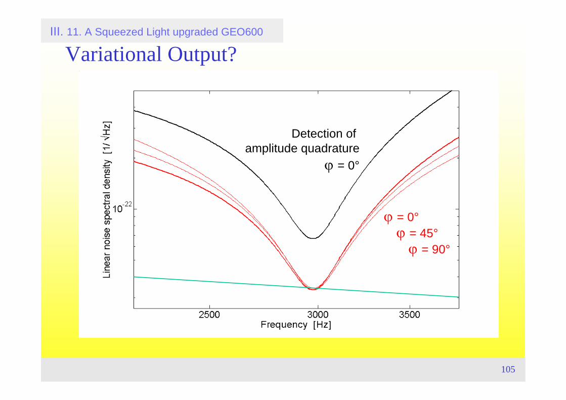
Amplitude quadratureϕ = 0°
ϕ = 0°
Amplitude quadratureϕ = 0°
ϕ = 0°ϕ = 45°
Detection of amplitude quadrature
ϕ = 0°
ϕ = 0°ϕ = 45°
ϕ = 90°
Variational Output?III. 11. A Squeezed Light upgraded GEO600
106
A Squeezed Light upgraded GEO600?
III. 11. A Squeezed Light upgraded GEO600
• Single filter cavity
• Squeezed light source
• Losses
• Proof of principle
107
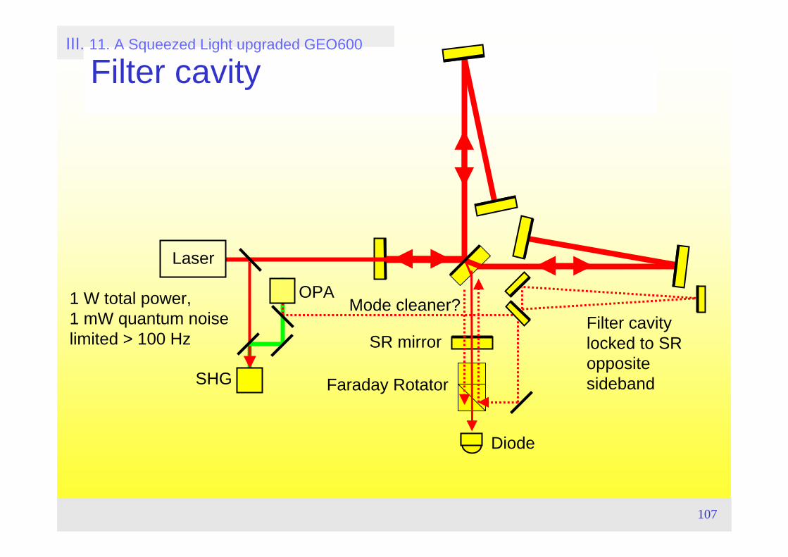
Filter cavity
Laser
Faraday Rotator
Diode
SHG
OPA
Filter cavity locked to SR opposite sideband
SR mirror
1 W total power, 1 mW quantum noise limited > 100 Hz
Mode cleaner?
III. 11. A Squeezed Light upgraded GEO600

108
III. 11. A Squeezed Light upgraded GEO600
109
III. 11. A Squeezed Light upgraded GEO600
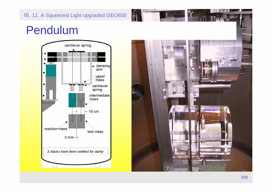
Pendulum
110
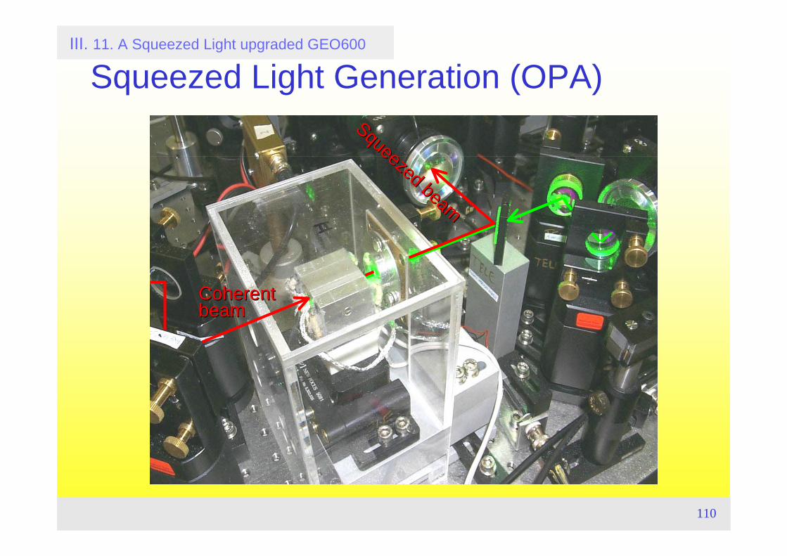
Squeezed Light Generation (OPA)Squeezed beam
Squeezed beam
Coherent Coherent beambeam
III. 11. A Squeezed Light upgraded GEO600
111
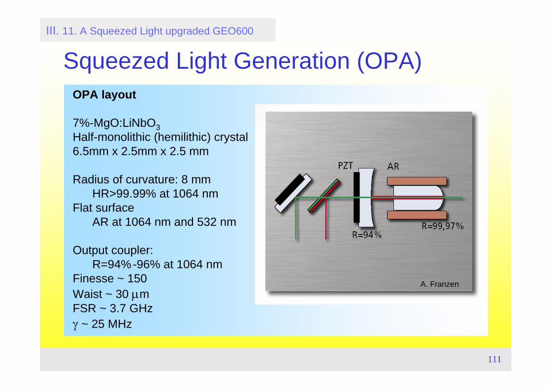
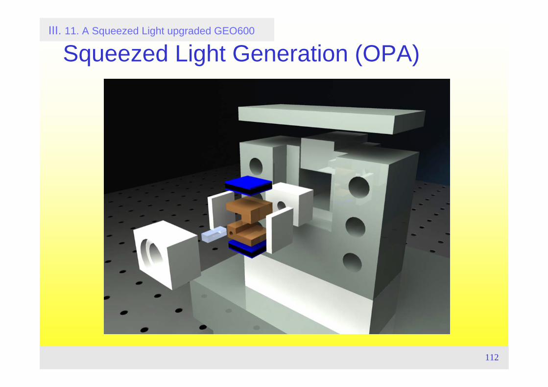
OPA layout
7%-MgO:LiNbO3Half-monolithic (hemilithic) crystal6.5mm x 2.5mm x 2.5 mm
Radius of curvature: 8 mm HR>99.99% at 1064 nm
Flat surfaceAR at 1064 nm and 532 nm
Output coupler: R=94%-96% at 1064 nm
Finesse ~ 150Waist ~ 30 μmFSR ~ 3.7 GHzγ ~ 25 MHz
A. Franzen
Squeezed Light Generation (OPA)III. 11. A Squeezed Light upgraded GEO600
112
Squeezed Light Generation (OPA)III. 11. A Squeezed Light upgraded GEO600
113
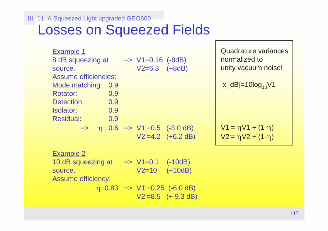
Losses on Squeezed Fields
Example 210 dB squeezing at => V1=0.1 (-10dB)source. V2=10 (+10dB)Assume efficiency:
η=0.83 => V1‘=0.25 (-6.0 dB)V2‘=8.5 (+ 9.3 dB)
Quadrature variances normalized to unity vacuum noise!
x [dB]=10log10V1
V1‘= ηV1 + (1-η)V2‘= ηV2 + (1-η)
Example 18 dB squeezing at => V1=0.16 (-8dB)source. V2=6.3 (+8dB)Assume efficiencies:Mode matching: 0.9Rotator: 0.9Detection: 0.9Isolator: 0.9Residual: 0.9
=> η= 0.6 => V1‘=0.5 (-3.0 dB)V2‘=4.2 (+6.2 dB)
III. 11. A Squeezed Light upgraded GEO600
114
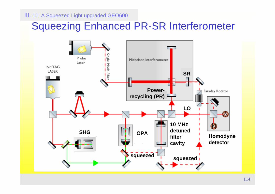
LO
Homodyne detector
SHG
squeezed
OPA DetunedFiltercavity
SR
Power-recycling (PR)
squeezed
Squeezing Enhanced PR-SR Interferometer
Homodyne detector
SHG
squeezed
OPA10 MHz detuned filter cavity
SR
Power-recycling (PR)
squeezed
LO
III. 11. A Squeezed Light upgraded GEO600
115
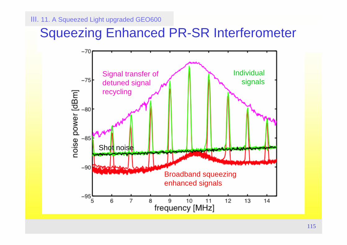
Squeezing Enhanced PR-SR Interferometer
Shot noise
Broadband squeezing enhanced signals
Signal transfer of detuned signal recycling
Individual signals
III. 11. A Squeezed Light upgraded GEO600
116
A Squeezed Light upgraded GEO600?
III. 11. A Squeezed Light upgraded GEO600
2008 !
117
III. Schemes for Nonclassical Interferometers 12. Speed Meter Idea and Sagnac Interferometer
TopicsMeasurement backactionQuantum-Non-Demolition (QND) measurements and variablesSpeed meterQND-Sagnac-gravitational wave interferometer
Literature• V. B. Braginsky and F. Ya. Khalili, Rev. Mod. Phys. 68, 1 (1996),
Quantum nondemolition measurements: the route from toys to tools.• Y. Chen, Phys. Rev. D 67, 122004 (2003),
Sagnac interferometer as a speed-meter-type, quantum-nondemolition gravitational-wave detector.
• P. Purdue and Y. Chen, Phys. Rev. D 66, 122004 (2002), Practical speed meter designs for quantum nondemolition gravitational-wave interferometers.
118
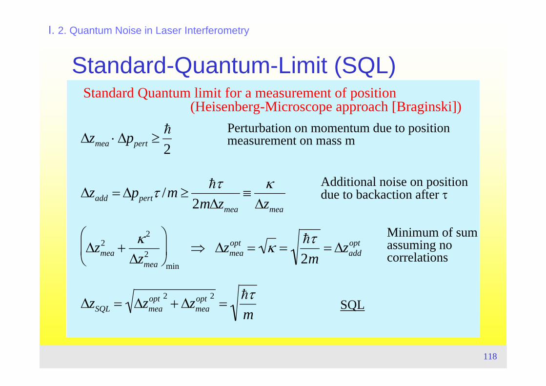
I. 2. Quantum Noise in Laser Interferometry
Standard-Quantum-Limit (SQL)
Δzmea ⋅ Δppert ≥h
2
Δzadd = Δppertτ /m ≥hτ
2mΔzmea
≡κ
Δzmea
Δzmea2 +
κ 2
Δzmea2
⎛
⎝ ⎜
⎞
⎠ ⎟
min
⇒ Δzmeaopt = κ =
hτ2m
= Δzaddopt
ΔzSQL = Δzmeaopt 2
+ Δzmeaopt 2
=hτm
Standard Quantum limit for a measurement of position(Heisenberg-Microscope approach [Braginski])
Perturbation on momentum due to positionmeasurement on mass m
Additional noise on positiondue to backaction after τ
Minimum of sum assuming no correlations
SQL

119
I. 4. Quantum Noise Spectral Densities
Standard-Quantum-Limit (SQL)
Δzmea ⋅ Δppert ≥h
2
Δzadd = Δppertτ /m ≥hτ
2mΔzmea
≡κ
Δzmea
Δzmea2 +
κ 2
Δzmea2
⎛
⎝ ⎜
⎞
⎠ ⎟
min
⇒ Δzmeaopt = κ =
hτ2m
= Δzaddopt
ΔzSQL = Δzmeaopt 2
+ Δzmeaopt 2
=hτm
Standard Quantum limit for a measurement of position(Heisenberg-Microscope approach [Braginski])
Perturbation on momentum due to positionmeasurement on mass m
Additional noise on positiondue to backaction after τ
Minimum of sum assuming no correlations
SQL

120
I. 3. Quantum Noise in Laser Interferometry
Shot Noise
SNR =1=dn2
Δn22
=sin φ /2( )cos φ /2( )α 2 dφ
α sin φ /2( )⇒ dφ =
1α cos φ /2( )
φ2
= 0 ⇒ dφ =1α
=1
ntotal
, Δφsn =1
ntotal
SNR =1=dn12
Δn122
=−sin φ( )α 2 dφ
α⇒ dφ =
1α sinφ
φ =π2
⇒ dφ =1α
=1
ntotal
, Δφsn =1
ntotal
Shot noise (coherent state noise) for a single detector at dark port
Shot noise for a differential detector at two half fringe ports
121
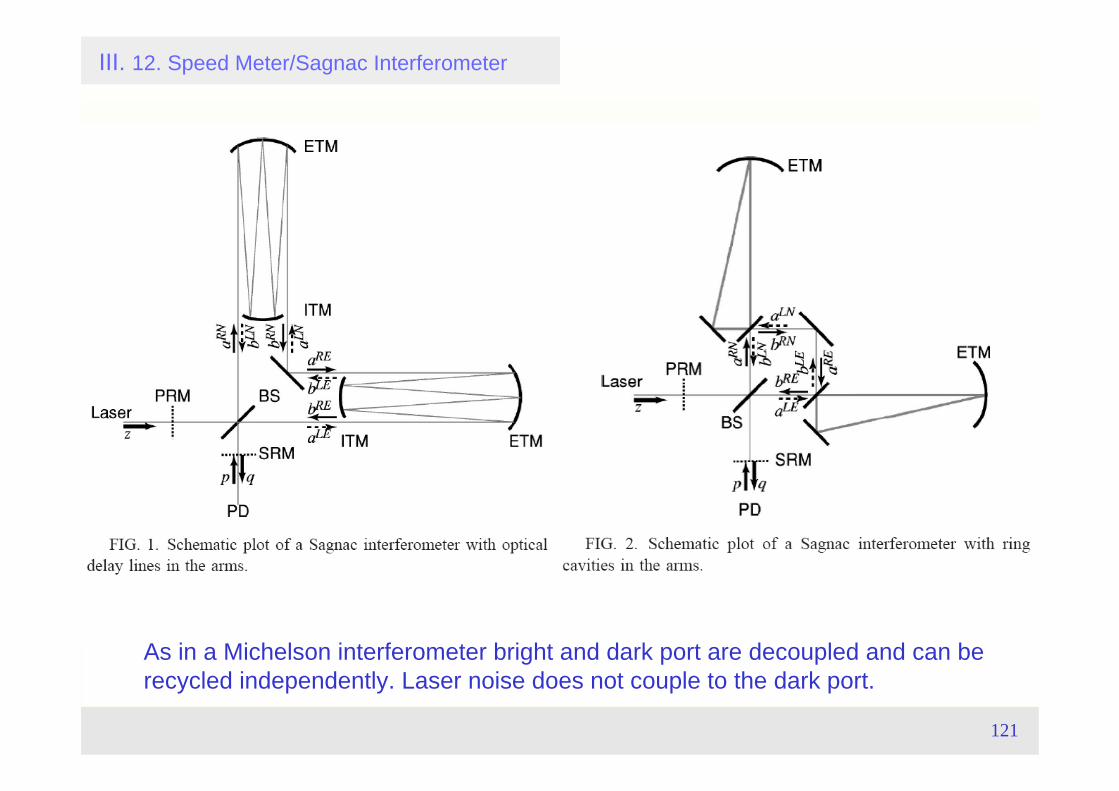
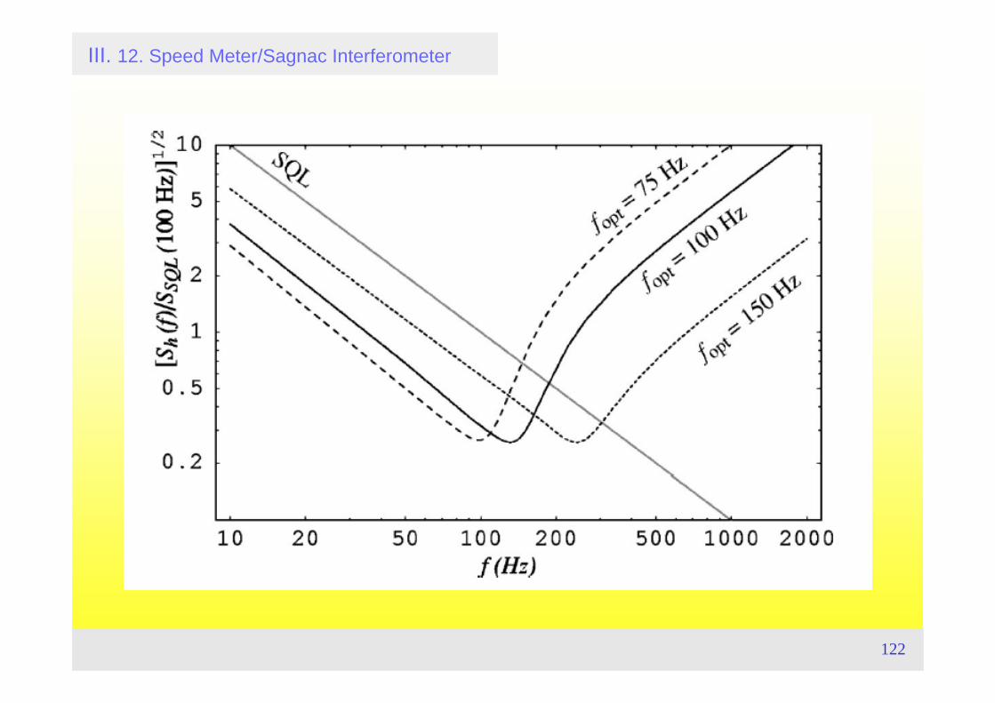
III. 12. Speed Meter/Sagnac Interferometer
As in a Michelson interferometer bright and dark port are decoupled and can berecycled independently. Laser noise does not couple to the dark port.
122
III. 12. Speed Meter/Sagnac Interferometer
123
III. Schemes for Nonclassical Interferometers 13. Optical Bars
TopicsOptical bar topology of a gravitational wave interferometerWeakly coupled oscillatorsThree-mirror-cavity QND and speed meter property of optical bar / leverHow does optical bar relate to the signal-recycling topology?
Literature• V. B. Braginsky, M. L. Gorodetsky and F. Ya. Khalili, Phys. Lett. A 232, 340 (1997)
Optical bars in gravitational wave antennas.• P. Purdue, Phys. Rev. D 66, 122001 (2002),
Analysis of a quantum nondemolition speed-meter interferometer.• V. B. Braginsky and F. Ya. Khalili, Rev. Mod. Phys. 68, 1 (1996),
Quantum nondemolition measurements: the route from toys to tools.
124
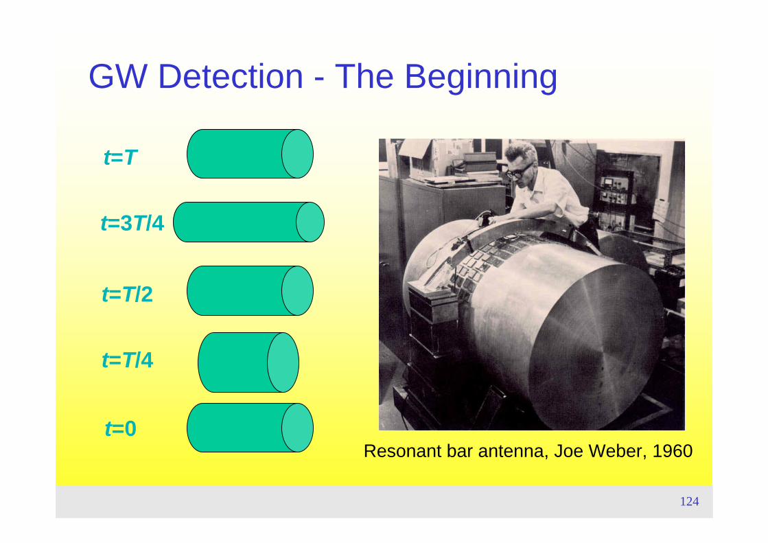
GW Detection - The Beginning
Resonant bar antenna, Joe Weber, 1960 t=0
t=T/4
t=T/2
t=3T/4
t=T
125
1990
1995
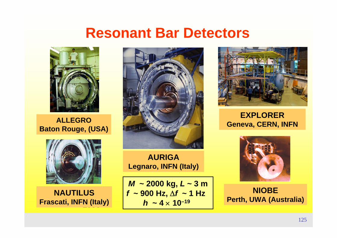
M ~ 2000 kg, L ~ 3 mf ~ 900 Hz, Δf ~ 1 Hz
h ~ 4 × 10–19
Resonant Bar Detectors
1991
ALLEGROBaton Rouge, (USA)
EXPLORERGeneva, CERN, INFN
NAUTILUSFrascati, INFN (Italy)
1993NIOBEPerth, UWA (Australia)
1997AURIGALegnaro, INFN (Italy)
126
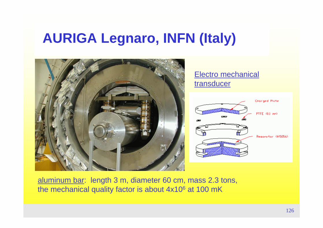
AURIGA Legnaro, INFN (Italy)
aluminum bar: length 3 m, diameter 60 cm, mass 2.3 tons,the mechanical quality factor is about 4x10⁶ at 100 mK
Electro mechanical transducer
127
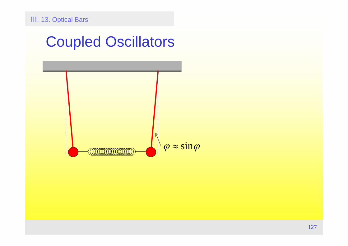
III. 13. Optical Bars
Coupled Oscillators
ϕ ≈ sinϕ
128
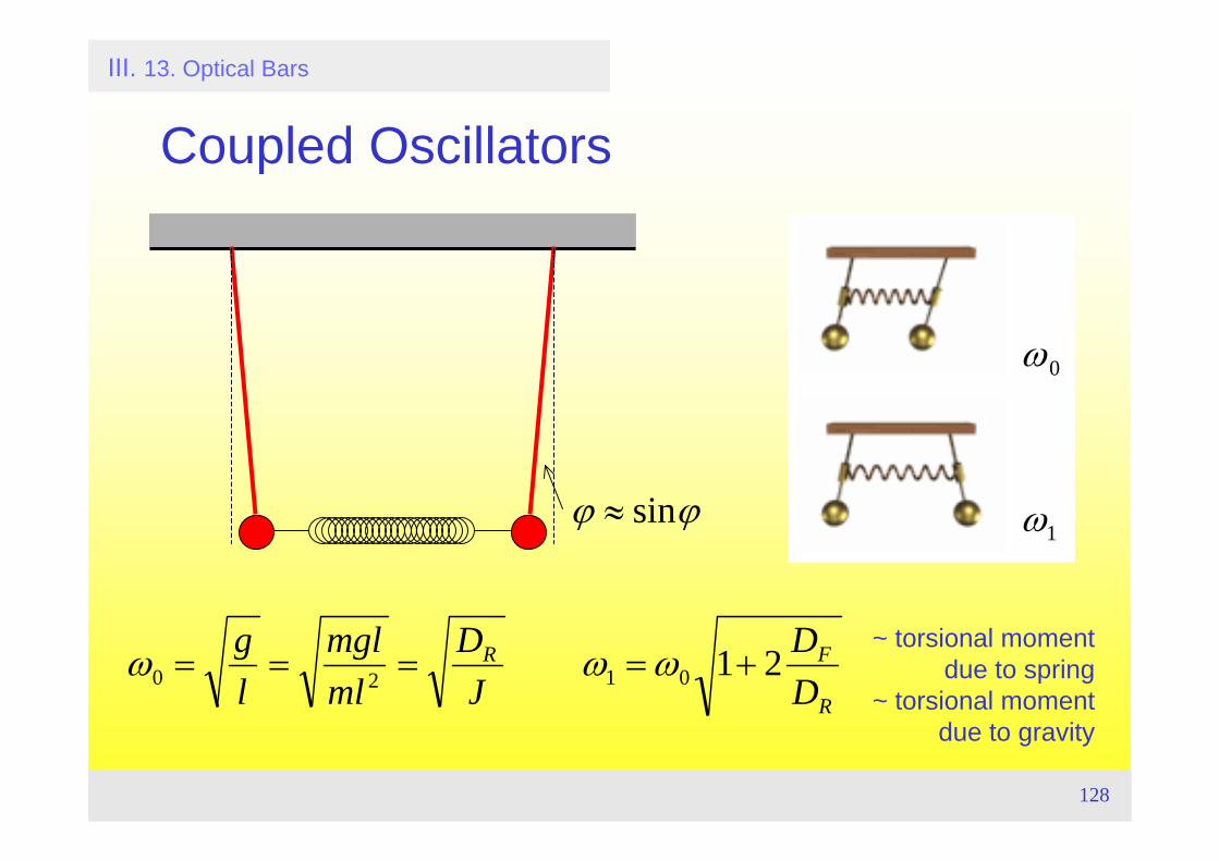
III. 13. Optical Bars
Coupled Oscillators
R
FR
DD
JD
mlmgl
lg 210120 +==== ωωω
~ torsional momentdue to spring
~ torsional momentdue to gravity
ϕ ≈ sinϕ ω1
ω0
129
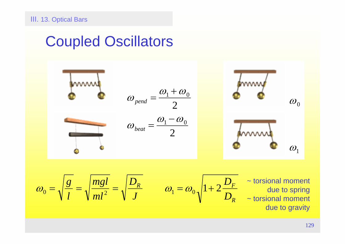
III. 13. Optical Bars
Coupled Oscillators
R
FR
DD
JD
mlmgl
lg 210120 +==== ωωω
~ torsional momentdue to spring
~ torsional momentdue to gravity
ω1
ω0ω pend =
ω1 + ω0
2
ωbeat =ω1 −ω0
2
130
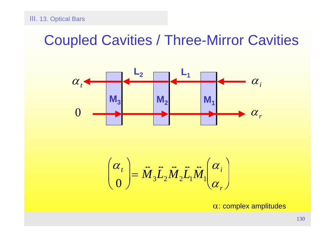
III. 13. Optical Bars
Coupled Cavities / Three-Mirror Cavities
α t
0⎛
⎝ ⎜
⎞
⎠ ⎟ =
t M 3
t L 2
t M 2
t L 1
t M 1
α i
α r
⎛
⎝ ⎜
⎞
⎠ ⎟
α t
0M3 M2 M1
L2 L1 α i
α r
α: complex amplitudes
131
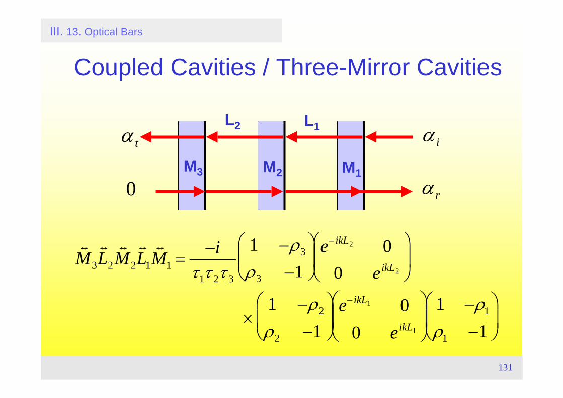
III. 13. Optical Bars
Coupled Cavities / Three-Mirror Cavities
t M 3
t L 2
t M 2
t L 1
t M 1 =
−iτ1τ 2τ 3
1 −ρ3
ρ3 −1⎛
⎝ ⎜
⎞
⎠ ⎟
e− ikL2 00 eikL2
⎛
⎝ ⎜
⎞
⎠ ⎟
×1 −ρ2
ρ2 −1⎛
⎝ ⎜
⎞
⎠ ⎟
e− ikL1 00 eikL1
⎛
⎝ ⎜
⎞
⎠ ⎟
1 −ρ1
ρ1 −1⎛
⎝ ⎜
⎞
⎠ ⎟
α t
0M3 M2 M1
L2 L1 α i
α r
132
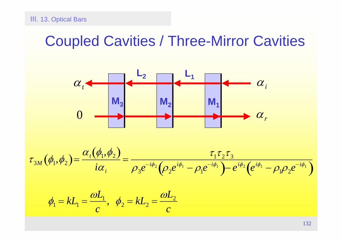
III. 13. Optical Bars
Coupled Cavities / Three-Mirror Cavities
τ 3M φ1,φ2( )=α t φ1,φ2( )
iα i
=τ1τ 2τ 3
ρ3e− iφ2 ρ2e
iφ1 − ρ1e−iφ1( )− eiφ2 eiφ1 − ρ1ρ2e
− iφ1( )
φ1 = kL1 =ωL1
c, φ2 = kL2 =
ωL2
c
α t
0M3 M2 M1
L2 L1 α i
α r
133
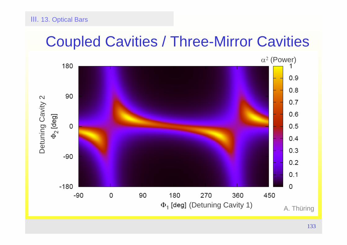
III. 13. Optical Bars
α2 (Power)
(Detuning Cavity 1)
Det
unin
g C
avity
2Coupled Cavities / Three-Mirror Cavities
A. Thüring
134
III. 13. Optical Bars
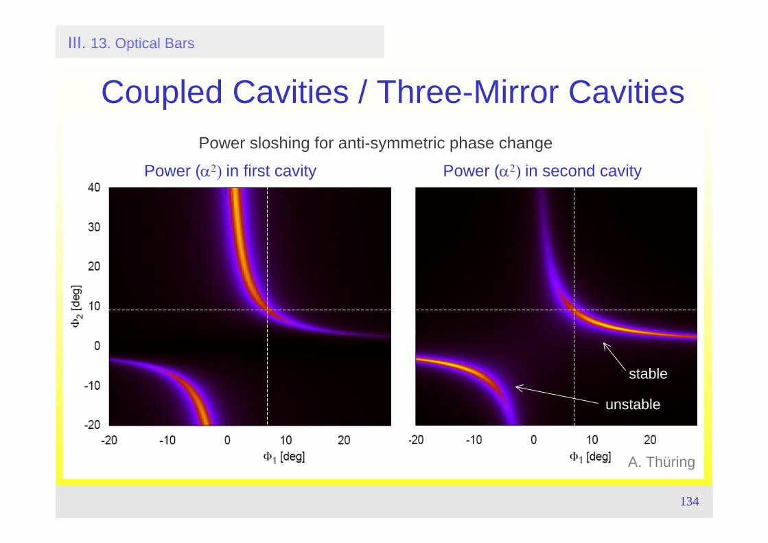
Coupled Cavities / Three-Mirror Cavities
A. Thüring
Power (α2) in first cavity Power (α2) in second cavity
Power sloshing for anti-symmetric phase change
stable
unstable