Time domain deBroglie wave interferometry

in a 2D trap

Saijun Wu1,2, Edward J. Su1, Mara Prentiss1

1. Department of Physics and Center for Ultra Cold atoms, Harvard University, Cambridge, MA, 02138

2. Division of Engineering and Applied Science, Harvard University, Cambridge, MA, 02138

PACS: 03.75.be, 32.80.-t, 42.50.Vk

Abstract: Time domain deBroglie wave interferometry [Cahn et al, Phys. Rev. Lett. 79, 784] is

applied to Rb87 atoms in a 2D linear trap. A standing wave light field is carefully aligned along the

guiding direction of the magnetic trapping potential generated by a soft-ferromagnetic 4-foil structure.

A sequence of two standing wave pulses is applied to the magnetically trapped atoms. The

backscattered light at the revival time is collected and detected via a heterodyning technique. Our

interferometer signal shows recoil oscillations that precisely fit the interferometer theory for atoms in

free space. We observe decay of the signal on a millisecond time scale , as well as millisecond scale

oscillations that suggest a residual variation of the linear trapping potential along the standing wave

direction.

1

I. Introduction:

An ability to coherently control the motion of atoms close to a surface may eventually lead to the

realization of chip-based atom interferometric devices for precise measurements and quantum

computing. Although significant progress has been achieved in developing the building blocks of

these devices, in most cases the external motion of the trapped atoms in the chip potential can be

modeled using only classical mechanics. [1-6]. A major difficulty associated with chip based atom

interferometry is the realization of a chip-based beamsplitter that generates a mutual coherence

between the trapped atoms [7, 8]. Atom beamsplitters are more difficult to create than atom traps or

guides because a potential that splits the trapped atoms needs to have sharp features comparable or

even smaller than the de Broglie wavelength of the trapped atoms, requiring either very cold atoms or

potentials that vary substantially over a micron. The size scale of the variation in the potential due to

an atom chip can be reduced by trapping atoms closer to the chip, but bringing atoms closer to the

chip surface can reduce interferometer performance because unwanted potential variations due to

fabrication errors become more important and the coupling of the atoms to various surface noise

channels increases [9, 10]. The problem is easily circumvented if the splitting potential is instead

generated by an optical standing wave above the chip surface, as demonstrated in a recent experiment,

where standing wave pulses coherently manipulated the guided motion of a Bose-Einstein condensate

on a chip [11].

A Bose condensed atom sample provides a sample size limited coherence length that may be

useful for interferometery; however, the atom-atom interactions of a condensate contribute additional

challenges to an interferometric experiment. In this paper we describe experiments using a trapped

2

atom sample that is far from quantum degeneracy, where we study the motion of the atoms in a 2D

magnetic trap using the time-domain deBroglie wave interferometry technique [12, 13]. At short times

scales (<< 1ms), our interferometer signal shows recoil oscillations in the contrast of the λ /2 atom

density grating due to the interference of guided atom wavepackets with themselves, which precisely

fits the predictions of interferometer theory for atoms in free space. The influence of the trapping

potential on the interferometer signal appears on a millisecond scale, when the motion of the atoms

along the standing wave direction is significantly perturbed by the residual trapping potential. This

time scale is set by the misaligning angle between the standing wave direction and the guide direction,

which cannot be adjusted to zero in this experiment due to the finite spreading of our atom sample

along the slightly curved guide. Nevertheless, our results indicate the feasibility of using standing

waves to coherently manipulate the guided motion of cold atoms in a magnetic trap. We also notice

that by confining the atoms in a guiding potential, the interrogation time of a light pulse atom

interferometer may be significantly increased, resulting in improvements in the sensitivity and

accuracy of guided measurements in comparison with those conducted in free space.

The remainder of the paper is organized in 3 parts. In part II we briefly review the theory of a

time domain de Broglie interferometer, and discuss the generalization of the formula to a magnetically

trapped atom sample. A formula that describes the leading order influence of a 2D linear trap on the

interferometer signal is then derived. In part III, we describe the experimental setup, and in part VI we

present the experimental results.

3

II. Time domain de Broglie wave interferometer with trapped atoms

Time domain deBroglie wave interferometry was first demonstrated by Cahn et al [12]: an

off-resonant standing wave made of two traveling light beams with wave vector k1 and k2 is pulsed on

an cold atom cloud twice, with pulse areas 1θ and 2θ separated by time T, before a probe light with

the wave vector k1 is switched on at time 2T+t and the backscattered light with the wave vector k2 is

collected and detected. We refer readers to [12, 13] for a detailed discussion on the theory of the

interferometer. Here we go directly to the expression for the backscattered signal.

Es(2T+t) ~ ),( tTi k∆ρ (1)

Where k∆ρ is the =k∆k 2-k1 Fourier component of the atom density distribution. For an atom

sample with spatial spreading much larger than the light wavelength and a thermal deBroglie

wavelength much smaller than the light wavelength, k∆ρ can be approximated with:

≈∆ ),( tTkρ ρ2)2/(

221 )]4(2[ kutr eTSintJ ∆−ωθθ (2)

Here ρ is the atom density, u is the mean thermal velocity of the atoms, rω is the angular recoil

frequency of the atom defined as mk

r 241 2∆

=ω where m is the mass of the atom. Thus

),( tTk∆ρ gives a dispersion-like curve as a function of t, the amplitude of which is modulated by the

second order Bessel function )]4(2[ 22 TSinJ rωθ , which is a periodic function of the interrogation

time 2T, with the periodrωπ

42

.

In the presence of a uniform linear potential V(s) = - m a s, where s measures the distance along

the standing wave direction, (1) is modified by including a phase factor

4

),( tTk∆ρ = ρ22 2)2/(

221 )]4(2[ kaTikutr eeTSintJ ∆∆−ωθθ (2’)

Thus the recoil frequency rω as well as the acceleration a can be measured by measuring the

backscattered light in repeated experiments while varying the interrogation time 2T and the probe time

t [14].

Unlike the case of a uniform linear potential where the potential variation preserves the amplitude of

the backscattered signal while shifting its phase, the presence of a general potential V(r) across the

atom sample usually degrades the amplitude of the backscattering signal. If V(r) is weak and smooth,

the leading order correction to the backscattering signal can be calculated by spatially averaging the

phase factor in (2’) across the atom sample:

),( tTk∆ρ = ρ2)2/(

221 )]4(2[ kutr eTSintJ ∆−ωθθ < >

22 VTkie ∇•∆r (3)

Equation (3) becomes a good approximation when V(r) is smooth enough such that for most atoms the

acceleration along the standing wave direction is a constant during the interrogation time 2T.

Our interferometer experiment confines atoms in a cylindrically symmetric magnetic field with a

field minimum at r=0. The standing wave direction, e.g., the direction of =k∆k 2-k1, is carefully

aligned to be parallel with the magnetic guiding direction. Thus equation (3) can be applied even in

the presence of tight transverse confinement. To illustrate the idea, consider an atom with magnetic

moment µ confined in a linear 2D magnetic guide with the magnetic field given in Cartesian

coordinates by B = . The confining potential can be written as V(r)

=

),,( 011 BxByB

20

22 ryxma ++ with 1Bma µ= and 1

00 B

Br = . Consider a standing wave with a wave

vector )1,0,(δk∆=∆k , where δ <<1 is the misaligned angle between the guiding direction z and

5

the standing wave direction. Assume the trapped atom sample has a Gaussian distribution with a

widthσ close to the magnetic field minimum, we have:

< >22 VTkie ∇•∆

r = 2

022

2

2

22 2

2

1 ryx

xkaTiyx

eedxdy ++∆+

−

∫∫δ

σ

πσ (4)

Integrating (4) in cylindrical coordinate gives:

< >22 VTkie ∇•∆

r = ∫∞

−

+

∆0

2

20

20 )

1

12( du

ur

kaTJe u

σ

δ (4’)

Where J0 is the 0th order Bessel function. If most atoms are in the linear region of the linear trap, e.g.,

σ >>r0, we end up with:

< > 22 VTkie ∇•∆ )

2)2((

2

0TkaJ ∆

≈δ

(4’’)

Together, (1), (3) and (4) imply that for 2D trapped atoms, the misalignment of the standing wave with

respect to the guiding direction introduces an additional modulation on the amplitude of the

backscattering signal as a function of 2T, that is oscillating and decaying on the time scale of

2T~ka∆δ

1. In particular, the amplitude of the backscattering signal should have a node at

2T0ka∆

≈δ

2.2, with which the argument in (4’’) equals the first zero of the Bessel function.

Before moving on to a detailed discussion of the experiment, we would like to emphasize that the

1D interferometer theory has to be applied to the magnetically trapped atoms with care. Although for

far off-resonant standing waves the influence of the Zeeman shift on the light shift potential can be

safely ignored, the tensorial nature of the pulsed light shift potential indicates a polarization dependent

6

pulse area across the trapped atom sample and possible spin-flips for atoms in weak field regions.

These unwanted nonlinear effects can be carefully avoided in different ways, and in particular, can be

eliminated for alkaline atoms by choosing linearly polarized, far-off - resonant light [15].

III. The Experimental setup

III.1 In situ loading of atoms in a magnetic guide[16]

We use a 4-foil magnetic structure to generate the 2D quadruple magnetic field for the 2D+

magneto-optical trap as well as the magnetic confining potential. The structure is composed of four

0.5mm thick, 65mm long by 31mm wide rectangularµ -metal foils that are placed parallel to each

other with 5mm separations (see fig.1a). The current sheets run through the wires around the foils pull

the 4 foils up and down alternatively to generate a 2D quadruple magnetic field on top of the 4-foil

structure. By increasing the magnetization of the two inner foils and the two outer foils in proportion,

the magnetic field gradient at the 2D field strength minimum can be varied while the position of the

minimum remains fixed.

About 108 Rb87 atoms are cooled and trapped from the background vapor by a 2D+

magneto-optical trap (MOT), 6mm away from the foil structure. In the last 12ms of the MOT

operation, first the magnetic field gradient ramps from 20G/cm to B1 (up to 100G/cm) in 10ms, while

the cooling laser intensity is reduced and detuned for polarization gradient cooling. The repumping

laser is switched off in the last 1ms before the MOT light is switched off, resulting in approximately 3

10× 7 atoms in F=1 hyperfine states trapped in the magnetic potential. The transverse width of the

atom distribution is around 200µ m at a magnetic gradient B1=50G/cm, and is inversely proportional

7

to B1. The trapped atoms have a mean longitudinal velocity u ~ 5cm/s that is roughly 8 times the recoil

velocity of the atoms. The guided motion of atoms in the magnetic trap can be studied by taking

absorption images from the side of the trap in repeated experiments, as shown in fig 1.b.

After the atoms have been transferred to the magnetic trap, we wait for a time tesc for the

untrapped atoms to escape the trap region, and perform the standing wave experiment with the

magnetically trapped atoms. tesc has been sampled from 3ms to 30ms, where tesc>9ms is enough to

eliminate the contribution of residual untrapped atoms to the backscattering signal.

III.2 The standing wave experiment

The standing wave is composed of two traveling laser beams that overlap at the atom trap region

with an intersection angle around 90mrad. The two beams, which will be referred as IΘ 1 and I2, are

independently controlled by acousto-optical modulators, and have a 1/e2 diameter of 4mm and 2mm

respectively. The standing wave light is 136Mhz blue detuned relative to the Rb87 D2 F=1 – F’=2

transition. While keeping the direction of I2 fixed, the direction of I1 can be adjusted to tune the

standing wave direction relative to the magnetic guide direction (see fig.2).

Two 600ns standing wave pulses separated by time T are applied to the atom sample. The pulse

area for both pulses are estimated to be θ =2.5. I1 is then switched on as the probe light from 2T-4µ s

for more than 100 µ s, during which the backscattered light is continuously collected with the

detecting optics. In a time-domain deBroglie wave interferometer experiment, the backscattered signal

light shares the same propagation direction as one of the traveling wave beams forming the standing

wave. The detecting optics setup requires extra care due to the fact that the traveling wave beam can

be orders of magnitude stronger than the signal light. In our experiment (see fig.2), a 40Mhz AOM is

8

used as a protective shutter before the detecting photodiode, and is switched on only when I2 is

switched off. Further, to detect the nanowatt level signal light, I2 is attenuated more than 70dB by

switching off its controlling AOMs during the probe time.

The backscattered light is mixed with an optical local field at a different frequency and collected

with a single-mode optical fiber that delivers the light to a fast avalanche photodiode (APD). The

mixed electronic signal from the APD is further mixed down to 40Mhz, and put into a Tektronix

digital oscilloscope. The amplitude of the backscattering signal is retrieved by using the oscilliscope’s

native FFT to measure the component of the electronic signal at frequencies near 40Mhz. The standing

wave experiment setup is summarized in fig.2; we also show a typical FFT signal from a single

iteration of the experiment. The time domain de Broglie interferometer is completed by varying the

interrogation time 2T in repeated experiment while recording the peak value of the FFT signal.

III.3 Automation

Standard laboratory automation techniques are used to simplify the process of observing the

backscattered light at different interrogation times 2T. The automation process used in this experiment

consists of three parts: two experimental control subprograms and a data reduction script.

The first subprogram is a LabView VI that provides the timing sequence for individual iterations

of the experiment. The MOT light intensity and frequency, repump light intensity, and magnetic coil

currents are controlled by a National Instruments PCI-6713 analog output card. Additionally, one of

the card’s analog outputs is used to provide a timed TTL trigger to initiate the standing wave sequence.

The second subprogram is a Visual Basic DLL that runs between iterations of the experiment. After

communicating with the oscilloscope to download the previous iteration’s FFT waveform, it averages

9

that waverform with the previous waveforms at the same inter-pulse spacing T. After performing the

required number of averaging, it performs a set of GPIB calls that set a new value for T and for related

parameters. The different values for T can be run in a random order to reduce the effects of slow

variations in the experimental conditions. Depending on the quality of the signal in different

experimental situation, the number of averaged iterations has been set from 2 to 36.

The data reduction script is a macro for Origin 7 that extracts the peak values of the

backscattering amplitude for each averaged FFT waveform. After doing this, it generates a spreadsheet

giving the amplitudes of the backscattering signals from experiments with different interrogation times

2T.

IV. Results and discussion

We begin the description of our experimental results with a data set that samples 2T from 0.2ms

to 0.6 ms in 2µ s separations (Fig. 3a). The standing wave experiments are taken out with B1=20G/cm

and tesc =3ms. Since the magnetic field is unaltered during the whole experiment, the experiment can

be repeated with a repetition rate as high as 5Hz. The recoil oscillation in Fig. 3 a) agrees well with the

theory described in part II, e.g., <|E(2T, t)|>t~ | )]4(2[2 TSinJ rωθ |. The optical pumping effect can be

included in the model described in part II by including a small imaginary part to the pulse area θ [17].

Fig 3d) shows a simulation result on the experimental curve based on the simply model with θ set to

be 2.6 + 0.08i. A comparison between the experimental curve in fig 3.b) and the simulation curve in

fig 3.d) shows that on a short time scale the backscattered signal is well described by the simple

interferometer model. A linear fit of the minimum backscattering signal time Tn with the recoil phase n

10

can be used to retrieve 0

2cos1

rr ωω Θ+= , where =0

rω 771.32 ×π kHz is the D2 line recoil

frequency of Rb87 atom. The intersection angle Θ between I1 and I2 has been measured to be 80 mrad

in this experiment. The fit in fig.3 b) yields the measured recoil frequency

|0rω exp= )001.0771.3(2 ±×π kHz. The result is consistent in different measurements with different

intersection angles . Θ

Given the time dependence of the backscattered signal derived above and the precise

measurement of the period of the oscillation, we can ignore the sub-millisecond scale recoil

oscillations and directly retrieve the longer time scale behavior by sampling the peak contrast point for

each oscillation. In particular, we see from fig3.a that at 2tn = 2Tn+ 8µ s the backscattering signal

reaches a peak in each recoil oscillation period. By sampling the backscattering signal with

interrogation time 2T around 2tn, we were able to study the millisecond scale behavior of the

backscattering signal with a small number of sampling points. The millisecond-scale experiments

were done with atoms prepared in different trapping potentials B1. In addition, the standing wave

direction was tuned relative to propagation direction in the magnetic guide by adjusting the I1

direction both horizontal and vertically. Typical experimental results are shown in fig. 4. The

oscillation and decay of the backscattering signal is clearly seen in all the data. To confirm that the

feature is due to the magnetically trapped atoms, we conducted a comparison experiment, where the

trapped atoms were moved to 1mm below the standing wave region by ramping up the magnetic bias

field during the escape time. As shown in fig. 5, the resulting amplitude of the backscattering signal is

below the noise level, indicating after a escape time of 10ms the residual untrapped atoms make a

negligible contribution to the trapped atom interferometer experiment.

11

More millisecond scale data with tesc=10ms are included in fig. 6, where we characterize the

decayed oscillation with 2T0 at the first node of the backscattering signal amplitude. We found that

B1T02 is approximately a constant as shown in fig. 7 a). Following the method described in part III, the

standing wave – guiding direction misalignment angle δ can be retrieved in each set of millisecond

scale data through the relation 2T0ka∆

≈δ

2.2. We adjusted the I1 around its optimal value and tried to

minimize the signal decay. By calculating the misaligning angleδ for each data set, the recorded data

sets can be represented by a point on the (δ ,Θ ) plane. Fig. 7b) gives such a plot that includes the

recorded data with I1 scans approximately horizontal along the I2 – guide plane. Notice the variation of

the calculated misaligning angle δ scales by roughly half that of the variation on the intersection

angle , as expected from the relation =kΘ ∆k 2-k1. However, we have not yet been able to reduce the

misaligning angle δ to less than 5mrad. This is unsurprising – the magnetic guide generated by the

4-foil structure is of course not perfectly straight. The edge fields from the ends of the 4-foils

effectively bend the magnetic guide vertically so that the guiding direction varies along a trapped atom

sample. The curvature of the guide in this experiment has been shown to be ~1m-1 in the magnetic

field simulations. Thus the guiding direction should vary up to 5mrad for a 5mm atom sample along

the guide, which could explain our inability to completely eliminate the effects of misalignment.

The influence of the waveguide curvature is not unavoidable. We are currently constructing a

new experimental apparatus with a longer magnetic structure that generates a much straighter guiding

potential. In addition, the influence of the waveguide curvature can be efficiently suppressed by

preparing the atom sample with much shorter spreading along the guide.

12

V. Conclusion

In conclusion, we have studied the time domain de Broglie wave interferometer with atoms in a

2D linear magnetic trap. We observed millisecond-scale oscillations on the amplitude of the

backscattering signal that are due to the influence of the residual magnetic field confinement along the

standing wave direction. In this experiment, the precision of the standing wave alignment relative to

the guiding direction is limited by a non-negligible curvature of the guide itself that introduces

variation of the guiding direction along the atom sample. This limitation can be overcome by

localizing the atom sample in the guide and increasing the aspect ratio of the magnetic structure to

make the guide straighter. Orders of magnitude improvement in the precision of the standing wave

alignment should be possible for a localized atom sample in a straighter guide generated by currents in

micro-fabricated wires on atom chips, rather than the macroscopic ferromagnetic foils used in this

experiment.

Acknowledgement:

This work is supported by MURI and DARPA from DOD, NSF, ONR and U.S. Department of the

Army, Agreement Number DAAD19-03-1-0106.

Reference

[1] Hommelhoff P, Hansel W, Steinmetz T, Hansch TW, Reichel J, Transporting, splitting and merging

of atomic ensembles in a chip trap, NEW JOURNAL OF PHYSICS 7: Art. No. 3 JAN 11 2005

13

[2] Muller D, Anderson D, Grow R, Schwindt, PDD and Cornell E, Guiding Neutral atoms around

curves with Lithographically Patterned Current-Carrying Wires. Physical Review Letters, 83(25) 5193,

1999

[3] Dekker NH, et al, Guiding Neutral Atoms on a Chip, Physical Review Letters, 84(6)1124, 2000

[4] Cassettari D, Hessmo B, Folman R, et al. Beam splitter for guided atoms, PHYSICAL REVIEW

LETTERS 85 (26): 5483-5487 Part 1 DEC 25 2000

[5] Muller D, Cornell EA, Prevedelli M, Schwindt PDD, Wang YJ, Anderson DZ, Magnetic switch for

integrated atom optics, PHYSICAL REVIEW A 63 (4): Art. No. 041602 APR 2001

[6] Dumke R, Muther T, Volk M, Ertmer W, Birkl G, Interferometer-type structures for guided atoms

PHYSICAL REVIEW LETTERS 89 (22): Art. No. 220402 NOV 25 2002

[7] Andersson E, Calarco T, Folman R, et al. Multimode interferometer for guided matter waves

PHYSICAL REVIEW LETTERS 88 (10): Art. No. 100401 MAR 11 2002

[8] Girardeau MD, Das KK, Wright EM, Theory of a one-dimensional double-X-junction atom

interferometer, PHYSICAL REVIEW A 66 (2): Art. No. 023604 AUG 2002

[9] Leanhardt A.E., et al, Propagation of Bose-Einstein condensates in a magnetic waveguide, Phys.

Rev. Lett. 89(4) 040401, 2002

[10] Lin YJ, Teper I, Chin C, Vuletic V, Impact of the Casimir-Polder potential and Johnson noise on

Bose-Einstein condensate stability near surfaces, PHYSICAL REVIEW LETTERS 92 (5): Art. No.

050404 FEB 6 2004

[11] Ying-Ju Wang, et, al, An Atom Michelson Interferometer on a Chip Using a Bose-Einstein

Condensate, Phys. Rev. Lett., 94, 090405 (2005)

14

[12] S.B. Cahn et al, “Time Domain De Broglie Wave interferometry”, Physical Review Letters, 79,

784, (1997)

[13] D. V. Strekalov, Andrey Turlapov, A. Kumarakrishnan, and Tycho Sleator, Periodic structures

generated in a cloud of cold atoms, PHYSICAL REVIEW A 66, 023601, 2002

[14] It can be shown that ),( tTk∆ρ can be monitored with a weak probe light continuously in t

without significantly perturbing the dynamics of the density grating. The discussion on this will be

given in a future publication.

[15] Mathur BS and Happer W, Light Shifts in the Alkali Atoms, Physics Review, 171(1) 11, 1969

[16] Vengalattore M, Rooijakkers W, Prentiss M, Ferromagnetic atom guide with in situ loading,

PHYSICAL REVIEW A 66 (5) 053403, 2002

[17] It can be shown that, by including an imaginary part to the pulse area θ , the Bessel functions

involve in the equation (2) follows following replacing rule: )]4(2[ TSinJ rn ωθ is replaced by

2/22 )]([ nn yx

yxyxJ−+

− , with x=2 Real [θ ] ]4[ TSin rω , y= 2 Imag [θ ] ]4cos[ Trω

15

Fig.1 the 4-foil structure, 2D+ MOT and the standing wave setup. (a) Cross-section of the 4-foil

structure: a 2D quadruple field is generated by the four-foil structure. A mirror MOT in 2D+

configuration is setup on top of the structure. Also included in a) is a calculated field and contour plot

of the magnetic field distribution. (b). The side-view of the 4-foil structure. On top of the structure the

position of the atoms and standing wave are indicated. Four absorption images taken at 5ms, 10ms,

20ms, and 30ms after the MOT light is switched off are shown on the top.

16

Fig.2 The interferometer setup. I1 and I2 intersect at the atom trap region to form a standing wave. The

angle between the two laser beams is around 90mrad, and is measured to 1% precision for each

experiment. By adjusting the direction of I

Θ

1, the direction of the standing wave relative to the magnetic

guiding direction can be adjusted. I1 and I2 are independently controlled via AOMs that are not shown

here. An inserted graph on the middle-right is a typical fft signal from a standing wave experiment.

WP: quarter-wave plate. PBS: polarization-dependent beamsplitter. BS: 95% transmission beam

pickoff. LO: local field. HP: high band-pass filter. LP: low band-pass filter.

17

Fig. 3 The interferometer data taken with atoms in B1=20G/cm 2D magnetic trap. The two traveling

laser beams that make the standing wave intersect with an angle measured to be 87mrad. (a) The recoil

oscillation, red arrows mark the time Tn for which the backscattering signal reaches a minimum. (b)

Expansion of the interferometer data around 0.52ms. (c) Fitting of Tn with n, Inset gives the fitting

error, which is smaller than 2 µ s for all the measured Tn. (d) A calculated backscattering signal based

on the model discussed in the main text.

18

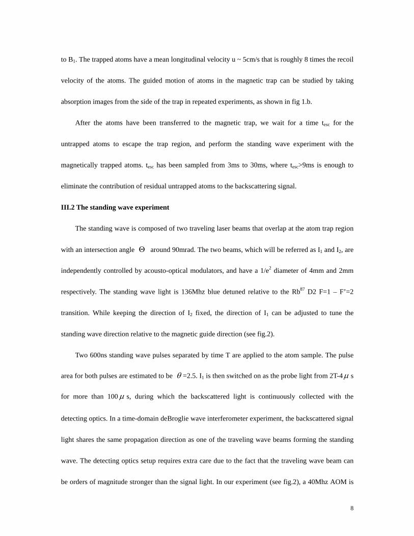
Fig.4. Millisecond-scale behavior of the interferometer signal. 2T is sampled at the peaks of each

recoil oscillation period. (a) and (c) are taken with two laser beams intersect with a angle Θ =

87mrad. While in (b) = 102mrad. (d) Θ Θ = 95mrad. Different magnetic field gradient B1 and the

untrapped atom escaping time tesc are also indicated in each figure.

19

Fig. 5, Comparison of the interferometer signals with (black dots) and without (red triangles) the

magnetic trapped atoms. Experimental condition: B1=30G/cm, tesc=10ms. Θ =95 mrad.

20

Fig. 6, Millisecond-scale behavior of the interferometer signal. The contrast oscillations in magnetic

guide with different magnetic confinements. tesc=10ms. Θ =95 mrad. The arrow in each graph

indicates the time 2T0 when the interferometer meets first millisecond scale contrast minimum.

21

Fig. 7 (a) the linear relation between 1/(2T0)2 and B1 retrieved from data in fig. 6. The 10%

uncertainty in the determination of T0 is reflected in the error bars along the y-axis. Relative

magnitude of B1 at each data point is determined by the current run through the conductors, and have

error bar smaller than the size of the symbols. (b) The misaligning angle δ is calculated from 14 set

of data taken with close to 90mrad, and plotted on the (Θ δ ,Θ ) plane. Different symbols represent

different B1 values. The 10% uncertainty in determination of T0 is reflected in the error bars of δ .

Intersection angle is measured to 1% precision in each experiment and the errors are smaller than

the size of the symbols here.

Θ

22