MICROARRAY DATA ANALYSIS TOOL USING JAVA AND R

By

Vasundhara Akkineni B.Tech, University of Madras, 2003

A Thesis Submitted to the Faculty of the

Graduate School of the University of Louisville In Partial Fulfillment of the Requirements

for the Degree of

MASTER OF SCIENCE

Department of Computer Engineering and Computer Science University of Louisville

Louisville, Kentucky

May 2006

MICROARRAY DATA ANALYSIS USING JAVA AND R

By

Vasundhara Akkineni B.Tech, University of Madras, 2003

A Thesis Approved on

April 14, 2006

By the following Thesis Committee:

Dr. Eric C. Rouchka, Thesis Director

Dr. Dar-jen Chang

Dr. Thomas Knudsen

ii

DEDICATION

Dedicated to my parents

Mr. Sarat Kumar Akkineni

and

Mrs. Surya Rani Akkineni

Thanks for everything, papa and ma.

iii

ACKNOWLEDGEMENTS

First, I would like to thank my thesis director, Dr. Eric C. Rouchka for his direction,

assistance and guidance. I would also like to thank the members of my thesis committee,

Dr. Dar-jen Chang and Dr. Thomas Knudsen for their time. I thank Tim Hardin,

Elizabeth Cha, Yamini Rudraraju and Eric Stutzenberger for making the Bioinformatics

lab an enjoyable place to come to each day. Additional thanks to the other members of

the Bioinformatics Research Group. I thank all the friends I have made over the years at

the University of Louisville. I have learned a lot from each one of you. Finally, I thank

my parents with all due respect for their love, support and encouragement. Support for

this project was provided by NIH-NCRR grant # P20 RR16481 (Nigel Cooper, PI).

iv

ABSTRACT

MICROARRAY DATA ANALYSIS USING JAVA AND R

VASUNDHARA AKKINENI

APRIL 14, 2006 Microarray technology has become an essential tool in functional genomics for

monitoring the expression of many genes in parallel. Gene expression values obtained

from microarray experiments help biologists to understand the way in which a cell

responds to varying conditions (including, but not limited to development over time,

response to environmental stimuli, or disease states) by analyzing the increase or

decrease in the expression level of genes. We have developed web-based software that

provides biologists with several statistical solutions for analyzing gene expression data.

This platform independent java servlet first performs normalization of the gene

expression values in order to eliminate any systematic bias in the measured intensity

values arising from the microarray process. Several normalization methods like Total

Intensity Normalization, Median Normalization and Lowess Normalization have been

implemented. After normalization, visualization of the experimental data can be

performed using scatter plots, MA plots, RI plots and image maps of the intensity ratios.

For detection of genes which are differentially expressed the software provides fold-

change detection and t-test techniques. The tool also provides the users the ability to

create a workflow of the different analysis tools used to study the uploaded

v

data. All the statistical routines used in this software were developed in R called from

Java code. This software is a freely available tool to statistically analyze microarray

experiments.

vi

TABLE OF CONTENTS

DEDICATION……………………………………………………………………………iii ACKNOWLEDGEMENTS………………………………………………………………iv ABSTRACT……………………………………………………………………………….v LIST OF TABLES………………………………………………………………………..xi LIST OF FIGURES...…………………………………………………………….……...xii 1. INTRODUCTION ...................................................................................................... 1

1.1 Overview of molecular biology .......................................................................... 4

1.2 DNA.................................................................................................................... 4

1.3 RNA .................................................................................................................... 6

1.4 mRNA................................................................................................................. 6

1.5 Gene .................................................................................................................... 7

1.6 Central Dogma of Molecular Biology ................................................................ 7

1.7 MicroRNA (miRNA) .......................................................................................... 8

1.8 Microarrays ......................................................................................................... 9

2. MICROARRAY ANALYSIS TECHNIQUES......................................................... 13

2.1 Microarray data analysis ................................................................................... 13

2.2 Log ratios .......................................................................................................... 16

2.3 Normalization ................................................................................................... 17

2.3.1 Total intensity normalization .................................................................... 17

2.3.2 Median normalization ............................................................................... 18

2.3.3 Lowess normalization ............................................................................... 18

2.4 Scatter plot ........................................................................................................ 19

vii

2.5 MA plot............................................................................................................. 20

2.6 RI plot ............................................................................................................... 21

2.7 Difference between MA and RI plots ............................................................... 22

2.8 Identifying differentially expressed genes ........................................................ 23

2.8.1 Fold change............................................................................................... 23

2.9 Clustering.......................................................................................................... 24

2.10 Types of clustering............................................................................................ 24

2.10.1 Hierarchical clustering .............................................................................. 25

2.10.2 Dendrogram .............................................................................................. 26

2.10.3 Heat maps.................................................................................................. 27

3. LITERATURE REVIEW ......................................................................................... 29

3.1 Bioconductor..................................................................................................... 29

3.2 TM4 and MIDAS.............................................................................................. 31

3.3 BASE: BioArray Software Environment.......................................................... 32

3.4 WebArray: an online platform for microarray data analysis ............................ 32

3.5 SNOMAD (Standardization and Normalization of MicroArray Data)............. 33

4. IMPLEMENTATION SPECIFICS .......................................................................... 35

4.1 R........................................................................................................................ 35

4.1.1 Statistics and R.......................................................................................... 36

4.1.2 R and Windows™..................................................................................... 36

4.2 Rserve ............................................................................................................... 37

viii

4.2.1 Installation of Rserve ................................................................................ 38

4.3 Java ................................................................................................................... 39

4.3.1 Java language ............................................................................................ 39

4.3.2 Java platform............................................................................................. 39

4.4 Java servlets ...................................................................................................... 40

4.5 JSP (Java Server Pages) .................................................................................... 42

4.6 JDBC (Java Database Connectivity)................................................................. 42

4.7 MySQL ............................................................................................................. 43

4.8 Apache Tomcat ................................................................................................. 44

5. OBJECTIVES AND RESULTS............................................................................... 46

5.1 Uploading experiment data ............................................................................... 47

5.2 Normalization methods..................................................................................... 48

5.3 Data visualization.............................................................................................. 50

5.3.1 Scatter plot ................................................................................................ 50

5.3.2 MA plot..................................................................................................... 51

5.3.3 RI plot ....................................................................................................... 52

5.4 Creating a process pipeline ............................................................................... 53

5.5 Identifying genes of interest.............................................................................. 57

5.5.1 Fold change cut-off ................................................................................... 57

5.6 Clustering genes................................................................................................ 60

5.7 Top and bottom intensity ratios ........................................................................ 61

ix

5.8 Search genes...................................................................................................... 63

5.9 Output results as files........................................................................................ 65

6. CONCLUSIONS....................................................................................................... 67

6.1 Possible improvements ..................................................................................... 68

REFERENCES…………………………………………………………………………..70

APPENDICES…………………………………………………………………………...72

CURRICULUM VITAE…………………………………………………………………77

x

LIST OF TABLES

Table 2.1 - Gene expression matrix with raw gene expression data................................. 14

Table 2.2 - Gene expression matrix with intensity ratio values........................................ 15

Table 2.3 - Gene expression matrix with log 2 intensity ratio values ............................... 16

Table 3.1 - Bioconductor packages................................................................................... 30

Table 5.1 - Color coding scheme for differentially expressed genes using fold change .. 57

xi

LIST OF FIGURES

Figure 1.1 - An overview of the formation of proteins....................................................... 4

Figure 1.2 - DNA double helix structure ............................................................................ 5

Figure 1.3 - Formation of mRNA ....................................................................................... 6

Figure 1.4 - Central Dogma of Molecular Biology............................................................. 8

Figure 1.5 - Preparation of microarrays............................................................................ 10

Figure 2.1 - Process of obtaining a gene expression matrix ............................................. 13

Figure 2.2 - Effects of lowess normalization .................................................................... 19

Figure 2.3 - A scatter plot ................................................................................................. 20

Figure 2.4 - An MA plot ................................................................................................... 21

Figure 2.5 - An RI plot...................................................................................................... 22

Figure 2.6 - Construction of a two-dimensional dendrogram representing a hierarchical

cluster of related genes...................................................................................................... 26

Figure 2.7 - A heat map with a dendrogram and a color key............................................ 28

Figure 4.1 - R command line interface on startup ............................................................ 37

Figure 4.2 - Java servlet execution process ...................................................................... 41

Figure 4.3 - The three-tier architecture of a JDBC connection......................................... 43

Figure 5.1 - Sample data file for analysis ......................................................................... 47

Figure 5.2 - Process of uploading data files...................................................................... 48

Figure 5.3 - Normalized data file using total intensity normalization .............................. 49

Figure 5.4 - Normalized data file using median normalization ........................................ 49

xii

Figure 5.5 - Total intensity normalization scatter plots and text files .............................. 50

Figure 5.6 - matrix of scatter plots with a zoomed out portion for two specific

experiments ....................................................................................................................... 51

nn×

Figure 5.7 - matrix of MA plots with a zoomed out portion for two specific

experiments ....................................................................................................................... 52

nn×

Figure 5.8 - matrix of RI plots with a zoomed out portion for two specific

experiments ....................................................................................................................... 53

nn×

Figure 5.9 - Steps for pipelining analysis ......................................................................... 54

Figure 5.10 - Pipeline screen to define a sequence of routines to be performed on the data

........................................................................................................................................... 55

Figure 5.11 - Results screen after submitting the pipeline screen .................................... 56

Figure 5.12 - Color based image map of the gene’s intensity ratios between two

experiments ....................................................................................................................... 59

Figure 5.13 – Individual gene details................................................................................ 59

Figure 5.14 - Heat map with a dendrogram to represent expression clusters ................... 61

Figure 5.15 - User selected columns for calculating the intensity ratios and the number of

top/bottom genes needed................................................................................................... 62

Figure 5.16 - Results showing top 10 ratios and bottom 25 ratios between two

experiments ....................................................................................................................... 63

Figure 5.17 - Search screen with the list of genes from the uploaded data file ................ 64

Figure 5.18 - Output screen for a search done on gene information................................. 65

xiii

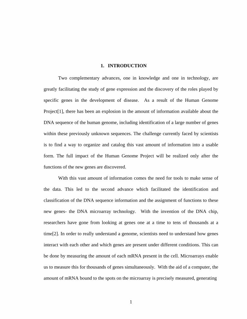
1. INTRODUCTION

Two complementary advances, one in knowledge and one in technology, are

greatly facilitating the study of gene expression and the discovery of the roles played by

specific genes in the development of disease. As a result of the Human Genome

Project[1], there has been an explosion in the amount of information available about the

DNA sequence of the human genome, including identification of a large number of genes

within these previously unknown sequences. The challenge currently faced by scientists

is to find a way to organize and catalog this vast amount of information into a usable

form. The full impact of the Human Genome Project will be realized only after the

functions of the new genes are discovered.

With this vast amount of information comes the need for tools to make sense of

the data. This led to the second advance which facilitated the identification and

classification of the DNA sequence information and the assignment of functions to these

new genes- the DNA microarray technology. With the invention of the DNA chip,

researchers have gone from looking at genes one at a time to tens of thousands at a

time[2]. In order to really understand a genome, scientists need to understand how genes

interact with each other and which genes are present under different conditions. This can

be done by measuring the amount of each mRNA present in the cell. Microarrays enable

us to measure this for thousands of genes simultaneously. With the aid of a computer, the

amount of mRNA bound to the spots on the microarray is precisely measured, generating

1

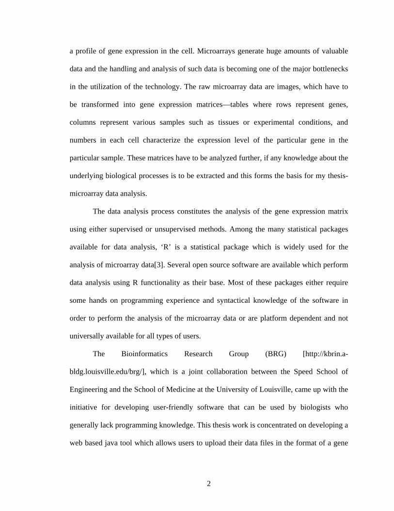
a profile of gene expression in the cell. Microarrays generate huge amounts of valuable

data and the handling and analysis of such data is becoming one of the major bottlenecks

in the utilization of the technology. The raw microarray data are images, which have to

be transformed into gene expression matrices—tables where rows represent genes,

columns represent various samples such as tissues or experimental conditions, and

numbers in each cell characterize the expression level of the particular gene in the

particular sample. These matrices have to be analyzed further, if any knowledge about the

underlying biological processes is to be extracted and this forms the basis for my thesis-

microarray data analysis.

The data analysis process constitutes the analysis of the gene expression matrix

using either supervised or unsupervised methods. Among the many statistical packages

available for data analysis, ‘R’ is a statistical package which is widely used for the

analysis of microarray data[3]. Several open source software are available which perform

data analysis using R functionality as their base. Most of these packages either require

some hands on programming experience and syntactical knowledge of the software in

order to perform the analysis of the microarray data or are platform dependent and not

universally available for all types of users.

The Bioinformatics Research Group (BRG) [http://kbrin.a-

bldg.louisville.edu/brg/], which is a joint collaboration between the Speed School of

Engineering and the School of Medicine at the University of Louisville, came up with the

initiative for developing user-friendly software that can be used by biologists who

generally lack programming knowledge. This thesis work is concentrated on developing a

web based java tool which allows users to upload their data files in the format of a gene

2

expression matrix and then performs normalization of the data, produces plots to

visualize the data, perform clustering of similar patterns of differentially expressed genes

and lets users to save their results to a text file.

It should be noted that a good understanding of these methods and the biology

behind the data is needed to choose the most appropriate for solving a particular problem.

The rest of chapter one is devoted to an overview of molecular biology, including a

discussion of DNA, RNA, genes and microarrays. Chapter two discusses microarray

analysis techniques, including an overview of log ratios, normalization, visualization

plots, differentially expressed genes using the fold change method, and clustering.

Chapter three is a literature review of existing microarray data analysis software, their

drawbacks and how the system being developed caters to the needs of the user who lacks

programming expertise. Chapter four gives a detailed description of the software used for

the development of the microarray analysis tool. Installation and implementation

specifics are also covered in a detailed manner. An overall discussion of the system being

developed in the form of its objectives and the results obtained is dealt with in chapter

five. Conclusions and further improvements to the microarray data analysis tool are

discussed in chapter six. A detailed glossary of terms is also available as part of this

thesis for the reader’s reference.

3

1.1 Overview of molecular biology

Every cell in an organism contains a full set of chromosomes and identical genes.

At a given point of time, only a subset of these genes is active. These genes define certain

unique properties of a cell type. The information contained in the DNA is transcribed into

messenger RNA (mRNA) molecules, which are then translated into proteins, which

perform most of the important functions of the cell. Figure 1.1 illustrates this process.

Cell Nucleus

Chromosome

Protein Gene (DNA)Gene (mRNA), single strand

Cell Nucleus

Chromosome

Protein Gene (DNA)Gene (mRNA), single strand

Figure 1.1 - An overview of the formation of proteins

1.2 DNA

Deoxyribonucleic Acid (DNA) is the basis for the building blocks encoding the

information of life. A single stranded DNA molecule, called a polynucleotide or

oligomer, is a chain of small molecules called nucleotides. There are four different

nucleotides, or bases: adenosine (A), cytosine (C), guanine (G) and thymine (T).

4

Stringing together a simple alphabet of four characters together we can get

enough information to create a complex organism. The ends of the polynucleotide are

marked either 3’ or 5’. The general convention is to label the coding strand from 5’ to 3’

(left to right). For instance, the following is a polynucleotide:

5’ G→T→A→A→A→G→T→C→C→C→G→T→T→A→G→C 3’

DNA can be either single-stranded or double stranded. When DNA is double-

stranded, the second strand is referred to as the reverse complement strand.

Complementary bases are determined by which pairs of nucleotides can form bonds

between them. In the case of DNA, A binds to T, and C binds to G. For the

polynucleotide given above, the double-stranded polynucleotide is as follows:

5’ G→T→A→A→A→G→T→C→C→C→G→T→T→A→G→C 3’

| | | | | | | | | | | | | | | |

3’ C←A←T←T←T←C←A←G←G←G←C←A←A←T←C←G 5’

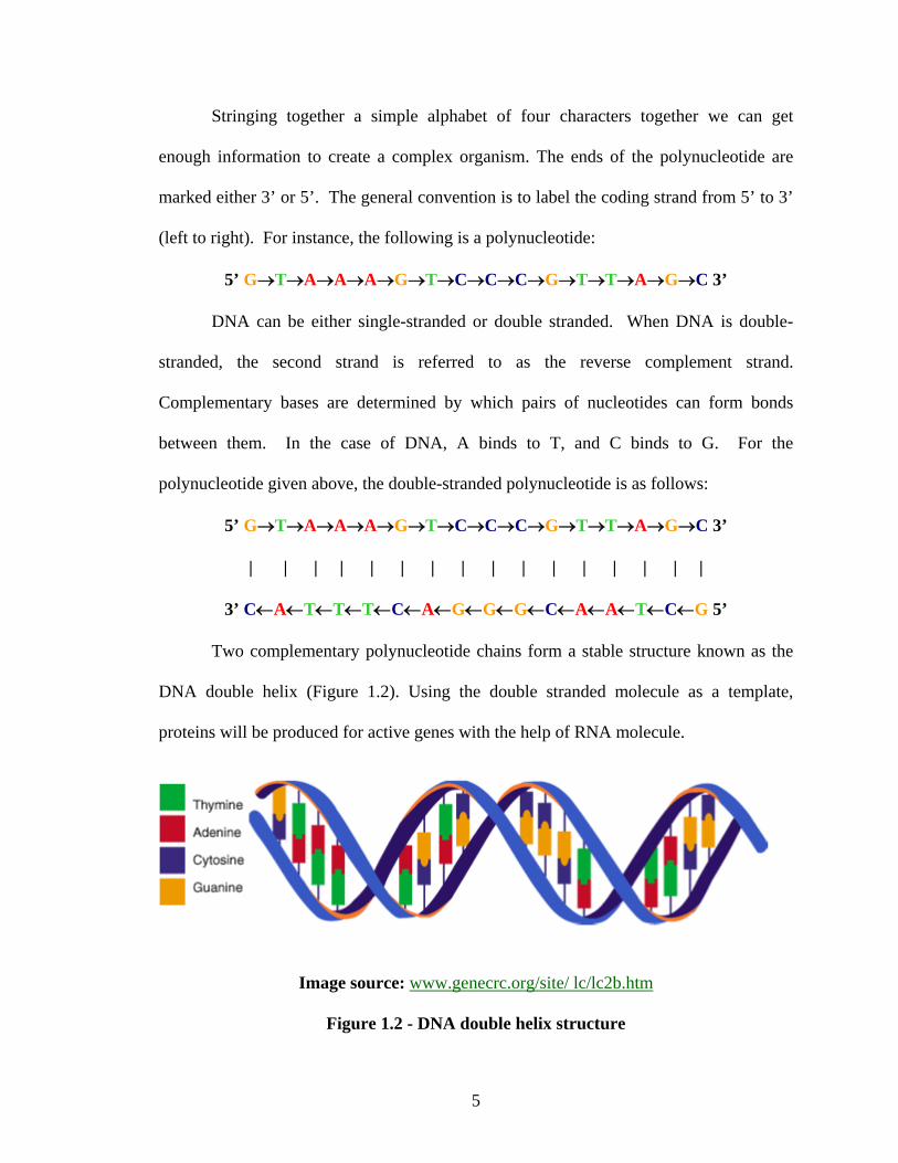
Two complementary polynucleotide chains form a stable structure known as the

DNA double helix (Figure 1.2). Using the double stranded molecule as a template,

proteins will be produced for active genes with the help of RNA molecule.

Image source: www.genecrc.org/site/ lc/lc2b.htm

Figure 1.2 - DNA double helix structure

5

1.3 RNA

Ribonucleic Acid (RNA) is similar to DNA in the fact that it is constructed from

nucleotides. However, instead of thymine (T), an alternative base uracil (U) is found in

RNA. RNA can be found as double-stranded or single-stranded, and can also be part of a

hybrid helix where one strand is an RNA strand and the other is a DNA strand. RNA is

important in the cell and contributes in a variety of ways. One of the most important

roles of RNA is in protein synthesis. Two of the major RNA molecules involved in

protein synthesis are messenger RNA (mRNA) and transfer RNA (tRNA).

1.4 mRNA

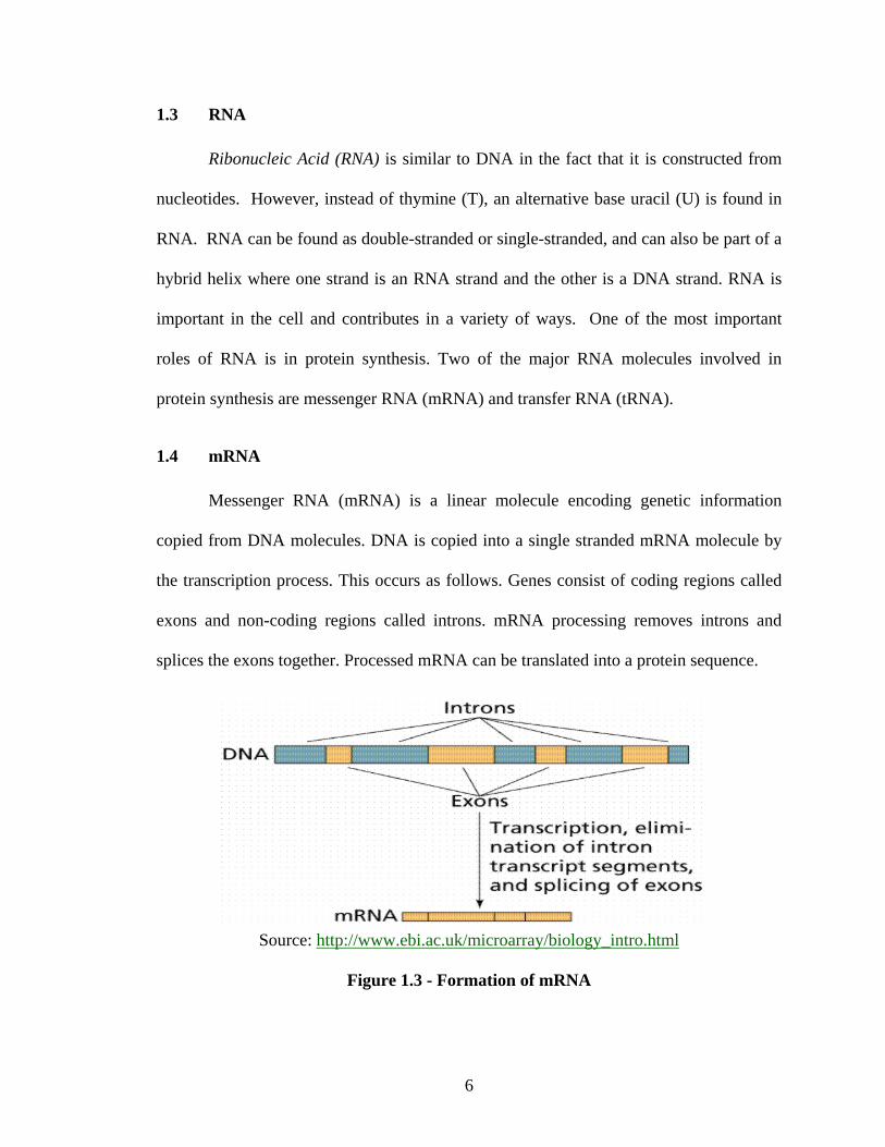
Messenger RNA (mRNA) is a linear molecule encoding genetic information

copied from DNA molecules. DNA is copied into a single stranded mRNA molecule by

the transcription process. This occurs as follows. Genes consist of coding regions called

exons and non-coding regions called introns. mRNA processing removes introns and

splices the exons together. Processed mRNA can be translated into a protein sequence.

Source: http://www.ebi.ac.uk/microarray/biology_intro.html

Figure 1.3 - Formation of mRNA

6

Therefore, in order to determine which genes are active in a cell (i.e., those that are

producing a protein product) one can measure the amount of mRNA present. This gives

an approximation of the activity of individual genes in a cell.

1.5 Gene

A gene can be described as the physical and functional unit of heredity that carries

information from one generation to the next[4]. A gene can be thought of as the DNA

sequence necessary for the synthesis of a functional protein or RNA molecule. Proteins

are important components of the body that determine how the different kinds of

molecules in the body are organized and act. Thus, proteins play a key role in the way we

look and the also in making us a unique individual. Genes are expressed as proteins, a

complex process consisting of two main steps: Each gene (DNA) is converted

(transcribed) into messenger RNA (mRNA), RNA that serves as a template for protein

synthesis. The resulting mRNA then guides the synthesis of a protein through a process

called translation. Thus isolating the mRNA helps us to find expressed genes from the

human genome.

1.6 Central Dogma of Molecular Biology

The Central Dogma of Molecular Biology states that the region of a double

stranded DNA molecule that corresponds to a gene is copied, or transcribed, to a

complementary single stranded mRNA molecule[5]. The single stranded mRNA

molecule then gets translated to a protein (Figure 1.4). If mRNA molecules can be

identified, the expression level of the corresponding genes can be determined.

7

Source: http://www.accessexcellence.org/RC/VL/GG/images/central.gif

Figure 1.4 - Central Dogma of Molecular Biology

1.7 MicroRNA (miRNA)

A miRNA is a form of single-stranded RNA which is typically 20-25 nucleotides

long, and is thought to regulate the expression of other genes[6]. miRNAs are RNA genes

which are transcribed from DNA, but are not translated into protein. The DNA sequence

that codes for a miRNA gene is longer than the miRNA. This DNA sequence includes the

miRNA sequence and an approximate reverse complement. When this DNA sequence is

transcribed into a single stranded RNA molecule, the miRNA sequence and its reverse-

complement base pair to form a double stranded hairpin loop which is a primary miRNA

structure (pri-miRNA). Pri –miRNAs are processed in the nucleus into hairpin RNAs

called Pre-miRNAs. The pre-miRNA molecule is then actively transported out of the

nucleus by a carrier protein. Thus through a mechanism that is not fully characterized, the

8

bound mRNA remains untranslated resulting in reduced expression of the corresponding

gene.

The function of miRNAs appears to be in gene regulation. miRNAs have been

reported to be critical in the development of organisms; they are differentially expressed

in tissues and are involved in viral infection processes. In the past two to three years, a

great deal of effort has gone in understanding how, when and where miRNAs are

produced and functions in cells, tissues and organisms. Several research groups have

provided evidence that miRNAs may act as key regulators of processes as diverse as

early development, cell proliferation and cell death, apoptosis and fat metabolism and cell

differentiation. There is speculation that the role of miRNAs in regulating gene

expression could be as important as that of transcription factors. The discovery of

miRNAs and their functions has added insight into how gene regulation is much more

complex than the Central Dogma of Molecular Biology previously led biologists to

believe.

1.8 Microarrays

Microarrays, developed in the lab of professor Patrick Brown at Stanford, in the

early 1990’s, took molecular biology by storm[7]. They are small slides spotted with

fixed samples of DNA, each for a different gene. When a researcher prepares a labeled

cell extract and incubates it with the slide, messengers in the sample anneal to the fixed

DNA, showing which genes in the sample are active. Microarray technology helps to

identify genes that are expressed under different conditions such as during the stages of a

cell cycle, under different environmental conditions, under diseased states at a particular

9

time, or under different tissue or cell types. A microarray is typically a glass slide, on to

which DNA, cDNA or Oligonucleotide molecules are attached at fixed locations (spots).

There may be tens of thousands of spots on an array, each containing a huge

number of identical DNA molecules of varying lengths. For gene expression studies, each

of these molecules ideally should uniquely identify a single gene in the genome.

Microarrays are used to compare gene expression levels in two different samples, for

example, a cell in a healthy state and a diseased state. A microarray employs the ability of

a given mRNA molecule to bind specifically to, or hybridize to, the complementary DNA

from which it is originated.

Source: http://www.bioteach.ubc.ca/MolecularBiology/microarray/index.htm

Figure 1.5 - Preparation of microarrays

10

A microarray contains many DNA sequences, and the expression levels of

thousands of genes can be determined in a single experiment by measuring the amount of

mRNA bound onto each spot of the array. Arranged systematically, the particular

sequences can be identified by the location of the spots on the slide.

For two channel experiments, the relative abundance of each of the gene-specific

sequences in two RNA samples (test and reference) may be estimated by fluorescently

labeling the samples, mixing them and hybridizing them to the sequences on the glass

slide. The two samples of mRNA from the cells (target) are reverse transcribed into

cDNA, and labeled using two different dyes (red Cyanine 5 and green Cyanine 3).

Usually, the reference sample is labeled Cy3 and the test sample with Cy5. The mixture

reacts with the spotted cDNA sequences (probes). This results in cDNA sequences from

the targets and the probes base-pairing with one another. After this hybridization step is

complete, the microarray is placed in a scanner, consisting of lasers with different

wavelengths, a microscope and a camera. The slide is scanned twice, first using one

colored laser and then the second. Laser light excites the fluorescent dyes, Cy3 is excited

by green laser light and Cy5 is excited by red laser light[4]. Green spots indicate that the

test substance has lower activity than the reference substance, red spots indicate that the

test substance is more abundant than the reference substance; yellow spots mean that

there is no change in the activity level between the two populations of test and reference

substance. Black represents areas where neither test nor control substance has bound to

the target DNA. The process of creating and labeling a microarray can be observed in

Figure 1.5.

11

Having an introduction to the central dogma of molecular biology, genes,

microarrays, their preparation process and uses, the next chapter introduces microarray

data analysis and the techniques used to analyze microarray data for obtaining useful

information and knowledge about the underlying biological processes.

12

2. MICROARRAY ANALYSIS TECHNIQUES

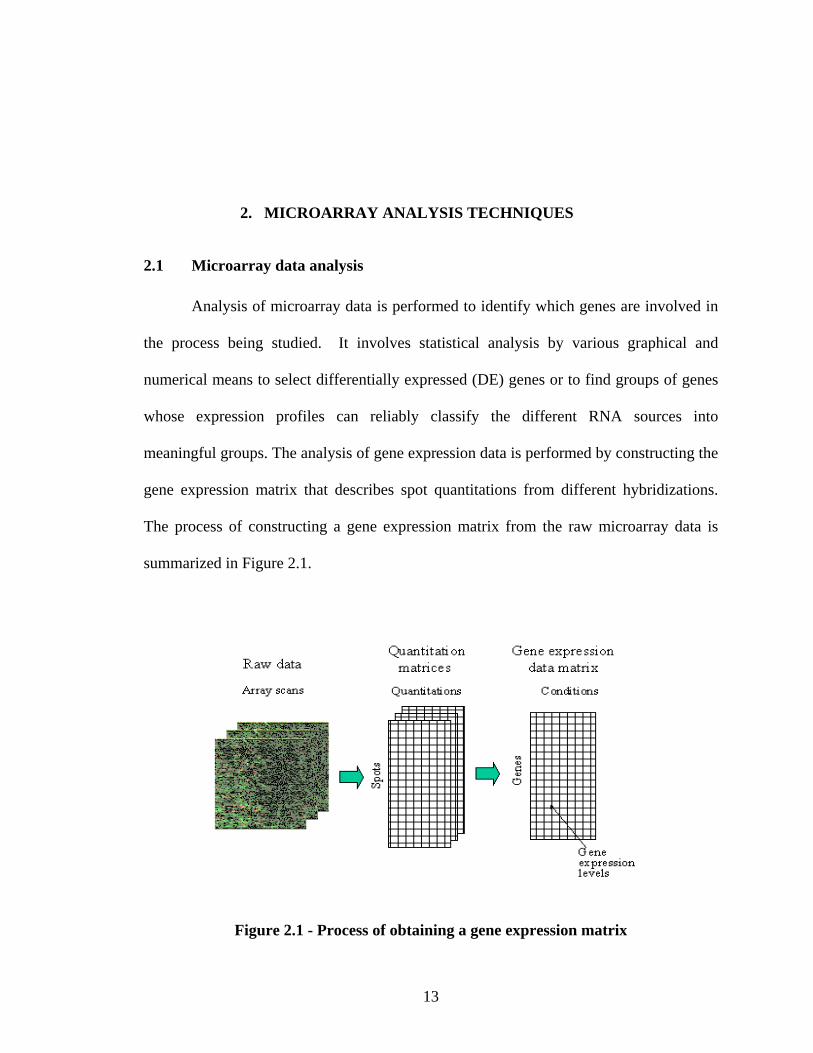
2.1 Microarray data analysis

Analysis of microarray data is performed to identify which genes are involved in

the process being studied. It involves statistical analysis by various graphical and

numerical means to select differentially expressed (DE) genes or to find groups of genes

whose expression profiles can reliably classify the different RNA sources into

meaningful groups. The analysis of gene expression data is performed by constructing the

gene expression matrix that describes spot quantitations from different hybridizations.

The process of constructing a gene expression matrix from the raw microarray data is

summarized in Figure 2.1.

Figure 2.1 - Process of obtaining a gene expression matrix

13

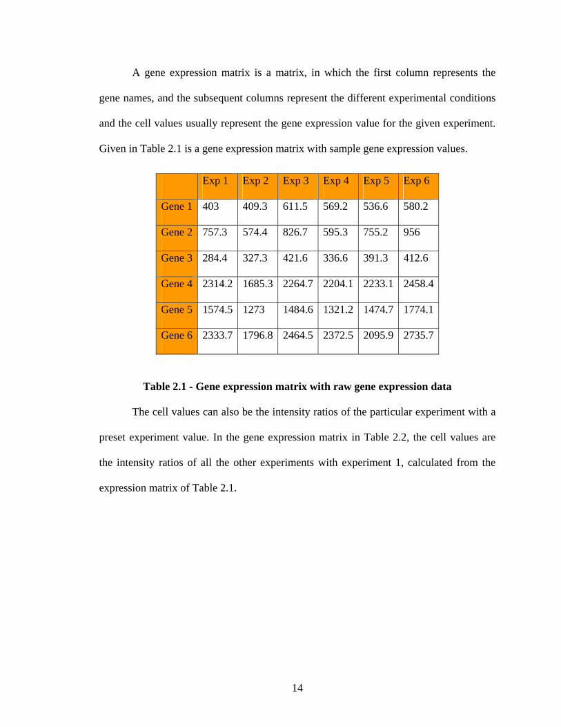
A gene expression matrix is a matrix, in which the first column represents the

gene names, and the subsequent columns represent the different experimental conditions

and the cell values usually represent the gene expression value for the given experiment.

Given in Table 2.1 is a gene expression matrix with sample gene expression values.

Exp 1 Exp 2 Exp 3 Exp 4 Exp 5 Exp 6

Gene 1 403 409.3 611.5 569.2 536.6 580.2

Gene 2 757.3 574.4 826.7 595.3 755.2 956

Gene 3 284.4 327.3 421.6 336.6 391.3 412.6

Gene 4 2314.2 1685.3 2264.7 2204.1 2233.1 2458.4

Gene 5 1574.5 1273 1484.6 1321.2 1474.7 1774.1

Gene 6 2333.7 1796.8 2464.5 2372.5 2095.9 2735.7

Table 2.1 - Gene expression matrix with raw gene expression data

The cell values can also be the intensity ratios of the particular experiment with a

preset experiment value. In the gene expression matrix in Table 2.2, the cell values are

the intensity ratios of all the other experiments with experiment 1, calculated from the

expression matrix of Table 2.1.

14

Exp 2/Exp 1 Exp 3/Exp 1 Exp 4/Exp 1 Exp 5/Exp 1 Exp 6/Exp 1

Gene 1 1.015633 1.51737 1.412407 1.331514 1.439702

Gene 2 0.758484 1.091641 0.786082 0.997227 1.26238

Gene 3 1.150844 1.482419 1.183544 1.375879 1.450774

Gene 4 0.728243 0.97861 0.952424 0.964955 1.062311

Gene 5 0.808511 0.942903 0.839124 0.936615 1.12677

Gene 6 0.769936 1.056048 1.016626 0.898102 1.172259

Table 2.2 - Gene expression matrix with intensity ratio values

Data analysis is based on the hypothesis that there are biologically relevant

patterns to be discovered in the data. The microarray data analysis process depends on the

analysis of the gene expression matrix using both supervised and unsupervised methods.

Most data analysis methods use raw expression values, intensity ratios or both for their

analysis routines. Data analysis methods take these huge sets of data as input and produce

both visual and numerical results for interpretation and further analysis. The most

commonly used microarray data analysis methods include log ratios of the gene intensity

data in order to spread the values across a given range, normalization to identify and

remove bias from the data, diagnostic plots of the microarray data for visualization

purposes, and methods to identify differentially expressed genes and clustering of genes

with similar behavior patterns. Each of these analysis techniques are discussed in detail in

the following sections.

15

2.2 Log ratios

A logarithmic transformation produces a continuous spectrum of values and treats

up and down regulated genes evenly across a range [8]. Equation 2.1 shows the formula

for calculating log2 ratios.

i

ii

GRX 2log= [Equation 2.1]

Where i=1, 2…..Ngenes and Ri , Gi are the measured intensity values for gene ‘i’ from two

different experimental conditions.

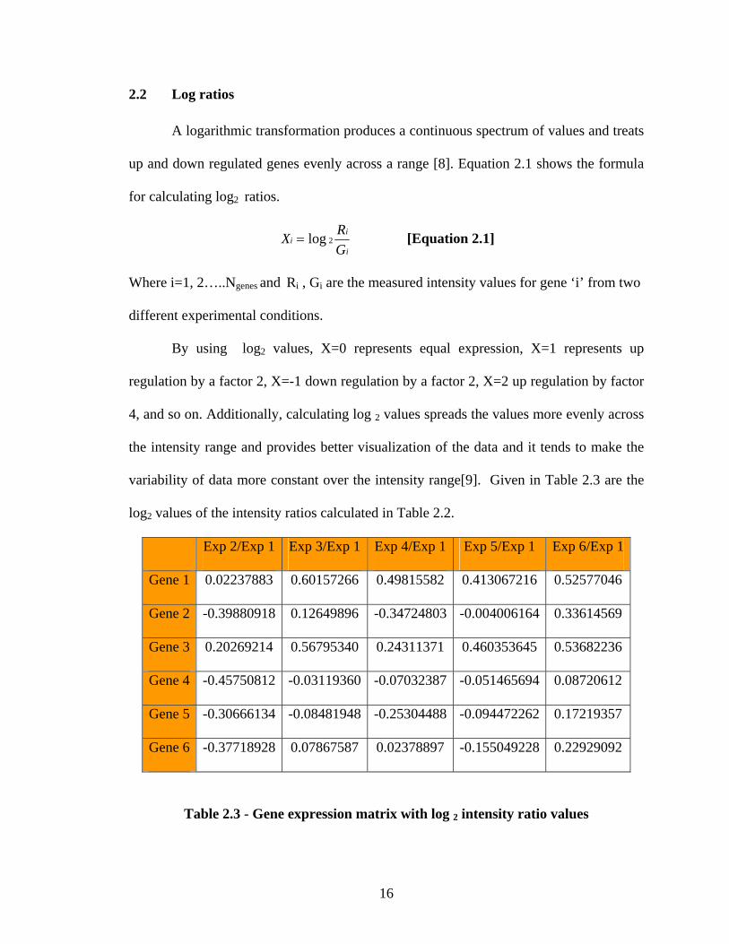
By using log2 values, X=0 represents equal expression, X=1 represents up

regulation by a factor 2, X=-1 down regulation by a factor 2, X=2 up regulation by factor

4, and so on. Additionally, calculating log 2 values spreads the values more evenly across

the intensity range and provides better visualization of the data and it tends to make the

variability of data more constant over the intensity range[9]. Given in Table 2.3 are the

log2 values of the intensity ratios calculated in Table 2.2.

Exp 2/Exp 1 Exp 3/Exp 1 Exp 4/Exp 1 Exp 5/Exp 1 Exp 6/Exp 1

Gene 1 0.02237883 0.60157266 0.49815582 0.413067216 0.52577046

Gene 2 -0.39880918 0.12649896 -0.34724803 -0.004006164 0.33614569

Gene 3 0.20269214 0.56795340 0.24311371 0.460353645 0.53682236

Gene 4 -0.45750812 -0.03119360 -0.07032387 -0.051465694 0.08720612

Gene 5 -0.30666134 -0.08481948 -0.25304488 -0.094472262 0.17219357

Gene 6 -0.37718928 0.07867587 0.02378897 -0.155049228 0.22929092

Table 2.3 - Gene expression matrix with log 2 intensity ratio values

16

2.3 Normalization

The goal of normalization is to identify and remove any systematic bias in the

measured fluorescence intensities, arising from variation in the microarray process rather

than from biological differences between the RNA samples or the printed probes[10;11].

Sources of bias include:

• labeling efficiencies of the dyes

• different amounts of Cy3 and Cy5 labeled mRNA

• scanning parameters

• spatial or plate effects, print tip effects, etc.

In the normalization process, a normalization factor (also referred to as scaling

factor) is calculated and is multiplied to all the values of an experiment. Either of the

experiments which are being compared can be multiplied with the normalization factor.

This process is the same as taking a constant value away from the log of the normal ratio.

2.3.1 Total intensity normalization

Total intensity normalization computes the normalization factor by summing the

measured intensities in both the experiments considered[10]. This is shown in Equation

2.2,

∑

∑

=

==array

kk

array

kk

totalN

G

NR

N

1

1 [Equation 2.2]

where Narray is the total number of genes, Gk and Rk are the measured intensity values of

the kth gene in both the experiments. The intensities are then rescaled such that Gk’ = Ntotal

17

Gk and Rk’= Rk and the normalized expression ratio for each feature are calculated

(Equation 2.3).

k

k

totalk

kk

GR

NGRT 1

''' == [Equation 2.3]

This is equivalent to

)(log)(log)'(log 222 totalkk NTT −=

2.3.2 Median normalization

In median normalization the normalization factor is found by calculating the

median of the array in question. Hence the equation becomes

akk medianTT −= )(log)'(log 22 where a is the experiment array.

The advantage of using the median normalization is that it is insensitive to outliers which

occur commonly in microarray data sets.

2.3.3 Lowess normalization

Lowess stands for Locally Weighted Linear Regression. It is also referred to as

Loess. Lowess uses a linear regression model whereas Loess uses a quadratic regression

model. The lowess normalization procedure subtracts a Lowess regression curve from the

data to normalize it[10;12].

18

Figure 2.2 - Effects of lowess normalization

A Lowess curve is first drawn on the RI Plot. The lowess curve is calculated by a

regression process which calculates the dependence of the ratio on the intensity and puts

it in a mathematical context.

The dependence, for each gene (i) is calculated by observing its distance

from the curve. On subtracting the dependence from the observed log

)( ixy

2 ratios, the

equation becomes:

))(^2(log)(log)()(log)'(log 2222 ikikk xyTxyTT −=>−= [Equation 2.4]

Figure 2.2 shows the effect of lowess regression on a set of data. The plot on the right

hand side is the RI plot itself and the plot on the left hand side is the RI plot fitted with

the lowess curve. Lowess detects the systematic deviations in the RI plot and corrects

them by carrying out a local weighted linear regression function given by Equation 2.4,

and uses this function, point by point, to correct the measured ratio values. The results of

applying such a lowess correction can be seen in the left hand side plot of Figure 2.2.

Lowess analysis is used as a normalization method that can remove intensity dependant

effects in the log2 ratio values.

2.4 Scatter plot

The scatter plot is an important graphical tool for studying the spread and linearity

of data[8]. In its simplest form, two variables are plotted along the axes, and marks are

19

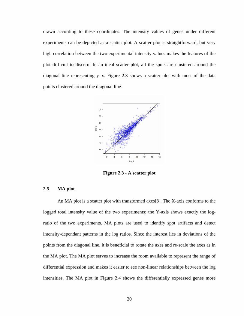
drawn according to these coordinates. The intensity values of genes under different

experiments can be depicted as a scatter plot. A scatter plot is straightforward, but very

high correlation between the two experimental intensity values makes the features of the

plot difficult to discern. In an ideal scatter plot, all the spots are clustered around the

diagonal line representing y=x. Figure 2.3 shows a scatter plot with most of the data

points clustered around the diagonal line.

Figure 2.3 - A scatter plot

2.5 MA plot

An MA plot is a scatter plot with transformed axes[8]. The X-axis conforms to the

logged total intensity value of the two experiments; the Y-axis shows exactly the log-

ratio of the two experiments. MA plots are used to identify spot artifacts and detect

intensity-dependant patterns in the log ratios. Since the interest lies in deviations of the

points from the diagonal line, it is beneficial to rotate the axes and re-scale the axes as in

the MA plot. The MA plot serves to increase the room available to represent the range of

differential expression and makes it easier to see non-linear relationships between the log

intensities. The MA plot in Figure 2.4 shows the differentially expressed genes more

20

clearly than the scatter plot in Figure 2.3. If an MA plot clearly shows the dependence of

the log ratio M on overall spot intensity A, this suggests that intensity or ‘A’ dependent

normalization method may be preferable.

Figure 2.4 - An MA plot

2log1log 22 ExpExpM −= )2log1(log21

22 ExpExpA +=

2.6 RI plot

A ratio-intensity (RI) plot is also a scatter plot like the MA plot that shows the

intensity specific effects for all the genes by plotting the log ratio as a function of the

product of the intensities[9;12]. RI plots are used to determine if there is a rough

correlation between the total intensity of a spot and its ratio. The easiest way to visualize

intensity-dependent effects, and the starting point for the lowess analysis described in

section 2.3.3, is to plot the measured log2 (Exp 1/Exp 2) for each gene as a function of the

log10 (Exp 1*Exp 2) product intensities. This ‘R-I’ plot can reveal intensity-specific

artifacts in the log2 (ratio) measurements which can be eliminated using lowess

21

normalization method. Under the assumption that most genes are not differentially

expressed, most of the points in the RI plot should fall along the horizontal line. Figure

2.5 shows an RI plot where a large number of genes which are not differentially

expressed fall along the horizontal line, and a number of differentially expressed genes

are scattered away from the horizontal line.

Figure 2.5 - An RI plot

2.7 Difference between MA and RI plots

The MA plot and RI plot are used to check if the data exhibits an intensity dependent

structure. RI plots and MA plots are used in an alternative manner by scientists.

In an MA plot, plot M=log 2 (R/G) Vs A= (1/2) log 2 (R*G)

In a RI plot, plot R= log 2 (R/G) Vs I=log 10 (R*G)

where R and G are two different experiments.

The type of plots used for analysis is a source of confusion due to the fact that the RI plot

looks very similar to an MA plot. It is important to know that MA plots are similar to RI

plots but are not the same. RI plots are most commonly used to show the effect of lowess

22

normalization. MA plots are used instead of scatter plots because they serve to increase

the room available to represent the range of differential expression and makes it easier to

see non-linear relationships between the log intensities.

2.8 Identifying differentially expressed genes

One of the main goals of microarray experiments is to identify differentially

expressed (DE) genes[11]. It will be practical to identify a limited number of genes which

are the most likely candidates. This set of DE genes can be further analyzed using

clustering techniques, etc.

2.8.1 Fold change

The fold change detection is a simple approach where a fixed fold-change-cutoff

interval is used to find genes which are differentially expressed.[10; 13]

21

sampleinvalueExpressionsampleinvalueExpressionchangeFold = [Equation 2.5]

If a gene’s experimental log-ratio exceeds the upper cutoff interval boundary, then

it is marked as significant and over expressed. If a gene’s experimental log-ratio falls

below the lower cutoff interval boundary, then it is marked as significant and under

expressed. Genes with experimental log-ratios in the range of the interval are marked for

regular behavior. Important factors to be considered in fold change method are what

cutoff should be used and should the cutoff be the same for all the genes. Though it is a

very straightforward method for classifying genes, the fold change method has the

disadvantage of not considering variability. Hence, genes with large variances are more

likely to make the cutoff just because of noise. For poorly expressed genes, small changes

23

in intensity can lead to large calculated fold changes. And it is not a statistically based

method.

2.9 Clustering

Microarray experiments deal with a large amount of data, which has to be stored

and analyzed. Therefore a general idea is to reduce the dimensionality of the data. The

basic concepts in clustering are to try to identify and group together similarly expressed

genes and then try to correlate and interpret the observations at the biological end. The

basic principles in gene clustering are:

1. Organize the data into a small number of homogeneous groups.

2. Find similar expression patterns of genes. Both low and high expression level

genes can be placed in the same cluster if their expression profiles have similar

shape.

2.10 Types of clustering

Clustering can be hierarchical or flat, as well as agglomerative or divisive[10].

Agglomerative processes start out by considering each object as a separate cluster and

proceed to group the most similar objects in an iterative fashion until all the data are

included. Divisive methods start out with the complete set of data as one large group, or

cluster, and proceed by partitioning the objects starting with those that are most

dissimilar. Based on their background principle, the different types of clustering methods

available are Hierarchical agglomerative clustering[9;10], Hierarchical divisive

clustering[9;10], k-means clustering and self organizing maps (SOM’s)[9;10;13].

24

2.10.1 Hierarchical clustering

The clustering method used for analysis in this tool is hierarchical clustering. The

hierarchical clustering algorithm uses a bottom-up approach where it iteratively joins the

two closest clusters starting from a single cluster[9;10;13]. After each step, a new

distance matrix between the newly formed clusters and the other clusters is recalculated.

For a set of N genes to be clustered, and a NN × distance matrix, the hierarchical

clustering is performed as follows:

1. Assign each gene to a cluster of its own.

2. Find the closest pair of clusters and merge them into a single cluster.

3. Compute the distances between the new cluster and each of the old clusters.

4. Steps 2 and 3 are repeated until all the genes are clustered.

The distance matrix is calculated by considering the shortest distance from any

member of one cluster to any member of the other cluster. Hierarchical clustering has

become popular for the following reasons:

• Hierarchical clustering techniques are meaningful to cluster data at the experiment

level rather than at the level of individual genes. Such experiments are most often

used to identify similarities in overall gene expression patterns in the context of

different treatment regimens.

• The analysis reveals groups of similar genes that can be studied in greater depth.

• It is possible to visualize the data in a hierarchical way using interactive computer

programs.

While intuitively appealing as a method, hierarchical clustering is not an efficient

method for very large gene expression matrices as the full distance matrix of all pair-wise

25

distances has to be calculated in advance, which for n objects takes an order of n2 steps.

Hierarchical clustering is also less suitable for noisy data.

2.10.2 Dendrogram

Hierarchical clustering can be represented as a tree called a dendrogram[9;10].

Source 1: http://www.awprofessional.com/articles/article.asp?p=357695&seqNum=4&rl=

Figure 2.6 - Construction of a two-dimensional dendrogram representing a hierarchical cluster of related genes

26

By cutting the dendrogram at a particular height will give the different clusters and the

ze of the clusters. The dissimilarity of the clusters is proportional to the length of the

ertical lines projecting from each cluster. Figure 2.6 is an example of how a dendrogram

f clusters is obtained.

Each column represents a different experiment, each row a different spot on the

icroarray. The height of each link is inversely proportional to the strength of the

orrelation. Relative correlation strengths are represented by integers in the

ccompanying chart sequence. Genes 1 and 2 are most closely coregulated, followed by

enes 4 and 5. The regulation of gene 3 is more closely linked with the regulation of

enes 4 and 5 than any remaining link or combination of links. The strength of the

orrelation between the expression levels of genes 1 and 2 and the cluster containing

enes 3, 4, and 5 is the weakest (relative score of 10). (Adapted from: Jeffrey Augen,

ioinformatics and Data Mining in Support of Drug Discover," Handbook of Anticancer

rug Development. D. Budman, A. Calvert, E. Rowinsky, editors. Lippincott Williams

2.10.3 Heat maps

A heat map is a color image with a dendrogram attached to the left side and to the

top of the image[10;14]. The rows and columns plotted in the heatmap are re-ordered

based on the restrictions imposed by the dendrogram. Each row in the heatmap represents

a gene and the columns represent the different experiments to which the gene is

subjected. The colors in the heat map simply represent the values in the gene expression

matrix. One can observe from a heat map (Figure 2.7) that genes with similar gene

expression profiles (i.e. strings of similar colors) are grouped close together.

si

v

o

m

c

a

g

g

c

g

"B

D

and Wilkins. 2003)

27

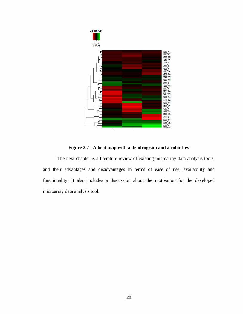
Figure 2.7 - A heat map with a dendrogram and a color key

The next chapter is a literature review of existing microarray data analysis tools,

and their advantages and disadvantages in terms of ease of use, availability and

functionality. It also includes a discussion about the motivation for the developed

microarray data analysis tool.

28

3. LITERATURE REVIEW

There are several commercial and non-commercial solutions as well as a growing

body of freely available open source software for analyzing microarray data. A review of

some popular open source microarray data analysis tools is presented here including

Bioconductor, TM4, MIDAS, BASE, WebArray and SNOMAD.

3.1 Bioconductor

Bioconductor is an open source project for computational biology[15]. The main

focus is to d on analysis.

Biocon

s at least one vignette, a document that provides a textual,

sk oriented description of the package’s functionality and can be used interactively.

lthough initial efforts focused primarily on DNA microarray data analysis, many of the

ftware tools are general and can be used broadly for the analysis of genomic and

xpression data. Bioconductor has adopted object-oriented programming as its primary

rogramming paradigm.

he main features of the Bioconductor project are:

Use of R to provide a wide range of statistical and graphical methods for the

analysis of genomic data.

eliver high-quality infrastructure and end-user tools for expressi

ductor is built completely on R[3;14] and R packages. A list of the different types

of packages available is given in Table 3.1. In addition to providing genomic data

analysis tools, Bioconductor has excellent integrated, dynamic documentation. Each

Bioconductor package contain

ta

A

so

e

p

T

29

Help integrate biological literature data from PubMed and LocusLink with the

analysis of genomic data.

Allows the development of extensible, scalable and interoperable software.

Provide high qual le research.

nalysis tool with a simple user interface, which does not require

the user upload data for analysis and

dow o the

web-ba e focus of this thesis.

ity documentation and reproducib

Provide training in computational and statistical methods for the analysis of

genomic data.

Task Packages

General programming tools Biobase, graph, tkWidgets, reposTools,

rhdf5

Annotation AnnBuilder,

Table 3.1 - Bioconductor packages

Although Bioconductor has the advantage of building on the existing toolkit of

statistical applications, it is command line based which is imposing for many users. The

tkWidgets package provides some functionality for creating GUI’s, but even that requires

additional programming.

The need for an a

annotate

Graphics Geneplotter, hexbin

Preprocessing microarray data Affy, marrayClasses, marrayInput,

marrayNorm, marrayPlots, marrayTools

Differential gene expression Genefilter, multtest, ROC

any kind of programming skills, and instead lets

nl ad the results in a point-and-click fashion, is the main factor in developing

sed application which is th

30

3.2

alysis suite of tools was developed to provide the

mic of the

mic ajor applications,

Mic a

System Multiexperiment Viewer (MeV). Since the focus of this project is

in array data analysis, the discussion is confined to MIDAS.

M alysis System

MIDAS is a java application which pr users an intuitive interface to design

an sses combining one or more ring steps. MIDAS

reads “.tav” (TIGR ArrayViewer file type, w mn, tab-delimited text

fo purposes o

a single slide) files generated by TIGR Spo ia

M les include lo ormalization. It

also includes background- ate analysis and filtering,

and the

s the data in tav format. While TM4 overcomes some of the

limitati

accessed through web, instead of

TM4 and MIDAS

The TM4 microarray an

roarray community with a comprehensive set of tools to handle all aspects

roarray process[16]. The TM4 suite of tools consist of four m

ro rray Data Manager (MADAM), TIGR_Spotfinder, Microarray Data Analysis

(MIDAS), and

micro

IDAS: Microarray Data An

ovides

alysis proce normalization and filte

hich is an eight-colu

rmat developed at TIGR for the f storing the intensity values of the spots on

tfinder or retrieved from the database v

ADAM. Normalization modu wess and total intensity n

and quality- control trimming, replic

identification of differentially expressed genes using intensity dependent Z-scores

and user defined fixed fold-change cut-offs. MIDAS provides scatter plots that illustrate

the effects of each algorithm on the data. When the normalization and filtering steps are

complete, MIDAS output

ons of a command-line driven system, it has the disadvantage of requiring users to

maintain current copies of the software locally and to update the system as it evolves.

Thus the need for an analysis tool which can accept data as a simple text file,

instead of program specific formats and which can be

31

maintaining local copies of the program on a user’s computer, has been another

motiva

BASE was developed using a web-based approach which closely integrates a data

management system with a data analysis system[16]. Since expression analysis tools are

evolving rapidly, BASE has a plug-in architecture that allows new modules to be easily

added for data transformation, analysis, or visualization. BASE incorporates a data

analysis interface that allows users to define an analysis method that passes data through

multiple routines and to create transformed datasets and subsets. This allows the original

unmodified data to be analyzed in a number of ways to create multiple analyses. BASE

allows data to be visualized in a variety of ways. Unmodified and transformed datasets

can be plotted interactively as scatter plots, displayed in histograms, or viewed as tables.

Though BASE minimizes the software update problem through its web-based approach,

it has the disadvantage that it loses a good deal of the graphical functionality that local

applications can provide.

The motivation for creating a pipeline process in the application being developed

comes from the analysis method of BASE. Also, though not yet implemented, the

integration of the data analysis module with a data management system as done in BASE

is a good future improvement.

ting fact in developing this application.

3.3 BASE: BioArray Software Environment

3.4 WebArray: an online platform for microarray data analysis

WebArray offers a convenient platform for biologists to access several cutting-

edge microarray data analysis tools[17]. WebArray runs on a LAMP system (Linux +

32

Apache + MySQL + Python) system. Background computations are mostly done by R

scripts. The currently implemented functions of WebArray were based on limma (Linear

Models for Microarray Analysis) and affy package from Bioconductor, the spacings

LOESS histogram (SPLOSH) method, PCA-assisted normalization method and genome

mapping method. WebArray incorporates these packages and provides a user-friendly

interface for accessing a wide range of key functions of limma and others, such as spot

quality weight, background correction, graphical plotting, normalization, linear modeling,

empirical bayes statistical analysis, false discovery rate (FDR) estimation, and

chromosomal mapping for genome comparison. Microarray analysis using WebArray can

be executed in three steps: 1) uploading and managing files; 2) selecting datasets and

methods for analysis, 3) browsing results. A good help document is also available with

detailed annotation of all the functions of WebArray. Thus WebArray is an excellent free

open source software for microarray analysis that can be used by an average biologist

after some training.

ardization and Normalization of MicroArray Data)

on to the regular transformations and visualization tools,

SNOMAD includes two non-linear transformations which correct bias and variance

which are non-uniformly distributed across the range of microarray element signal

intensities: 1) local mean normalization; and 2) local variance correction (Z-score

generation using locally calculated standard deviation).

3.5 SNOMAD (Stand

SNOMAD is an interactive, user-friendly web-application which can be accessed

freely via the internet with any standard HTML browser[18]. SNOMAD is a collection of

algorithms for the normalization and standardization of gene expression datasets derived

from diverse sources. In additi

33

The SNOMAD tool is available at -

http://pevsnerlab.kennedykrieger.org/snomad.htm. No programming expertise or

software installation is required. Users can upload their gene expression data and specify

the transformations they wish to apply on their data. Results come in the form of both a

text file containing numeric values and image files of graphs of the data corresponding to

all the transformations.

WebArray and SNOMAD are two user-friendly tools available in the market for

microarray data analysis. But they have their own disadvantage of having limited

functionality, confined to a certain set of routines that the user can perform on the data.

They do not have the scope for adding new R programs to the already existing system. In

such a case, biologists tend to use multiple tools for obtaining the required results. This

lack of extensibility formed another motivation for the development of the application

under discussion. Thus all these above discussed factors led to the development of the

current application to provide a solution to the community driven need for an easy to use,

readily available and extensible microarray data analysis tool, which uses R routines for

analysis.

34

4. IMPLEMENTATION SPECIFICS

In this chapter, the software implementation specifics for the microarray analysis

tool are discussed. A brief introduction to the R package, which forms the base for the

statistic

4.1 R

R is a powerful software environment for data manipulation, calculation and

graphical display. It is a GNU General Public License project similar to the S language.

The name is partly based on the first names of the first two authors (Robert Gentleman

and Ross Ihaka), and partly a play on the name of the Bell Labs language ‘S’[3;14].

supports a wide range of statistical techniques including descriptive statistics,

linear and nonlinear modeling, classical statistical tests, probability distributions, analysis

of variance (ANOVA), time series analysis, classification, clustering, robust regression

and maximum likelihood.

al analysis of the microarray data is given. Description of Java which has been

used to develop the user interface, and information about Rserve, which is the plug-in

used to connect to R from Java are also given. Some background about MySQL database

and the JDBC connection needed to connect to a database from Java code is also

provided. A clear understanding of the software is needed to understand the

implementation techniques discussed in this thesis.

R

35

R is extensible via user defined functions written in its own language, or through

the use of dynamically loaded modules written in other languages. It can be used with

Linux, UNIX and Microsoft Windows™.

4.1.1 Statistics and R

Most of the statistical techniques have been built into the base R environment and

many more are supplied in the form of packages. There are about 10 packages called

standard packages which are supplied with R and many more can be downloaded from

the Comprehensive R Archive Network (CRAN) website (http://cran.r-project.org).

The major difference between R and other statistical systems is that in R, the

statistical analysis is performed as a sequence of steps with the results of every step

stored in objects. In systems like SAS and SPSS copious output is obtained from a

regression or analysis whereas R will give minimal output and store the results in a fit

ct f further processing by R functions.

4.1.2 R and Windows™

The latest version of R for Windows™ can be downloaded from the CRAN

website. The version used for development of this project is R 2.1.1. A full installation of

R on Windows™ takes up to 50 MB of disk space. To install, double click on the icon for

rw2011.exe and follow the instructions. R installed in this way can be started from the

start menu or by double clicking the R shortcut. To add packages to the existing R

system, download the packages from the CRAN website and unzip them into the

R/rw2011/library folder directly.

obje or

36

Figure 4.1 - R command line interface on startup

erted into native data types.

• Persistent connections until the connection are closed.

4.2 Rserve

Rserve [19]is a TCP/IP server which allows other programs to use R facilities

from various languages without the need to initialize R or link against R library. Rserve

supports remote connection, authentication and file transfer. Typical use of Rserve is to

integrate R backend for computing statistical models, plots, etc from other applications.

The features of Rserve include:

• R initialization is not necessary.

• Most R data types are conv

37

• Offers client independence since the client is not linked to R.

• Rserve provides some basic security in the form of encrypted user/password

authentication.

• Rserve allows transferring files between the client and the server.

Rserve itself is the server which responds to requests from the clients. It listens

for incoming connections and processes incoming requests. A client framework was also

developed – JRclient. JRclient is a client suite which allows a java application to access

Rserve. It was developed in java. It provides automatic type translation for most objects

such as int, double, arrays, string or vector and classes for special R objects such as

RList, RBool, etc. The idea behind the separation of client/server side allows handling

multi-threading better when linking to R library directly.

4.2.1 Installation of Rserve

R 1.5.0 or to be able to use

AIX and Windows™. The Windows™ version

of Rserve was used for development. Although Rserve works on Windows™, it is not the

recommended since Windows™ lacks important features that make the separation of

namespaces possible. Therefore Rserve for Windows™ allows only one connection at a

time and all subsequent connections share the same namespace.

Installation process for Windows™:

1. Make sure to download the proper binary based on the version of R.

2. Copy the binary Rserve.exe to the same directory where R.dll is located. By

default it is in the R\rw2011\bin folder.

3. Run rserve.exe to start the server and to make connections to R.

higher needs to be installed on your system in order

Rserve. Rserve works on Linux, Solaris,

38

Rserve was developed by Simon Urbanek, a researcher at AT&T Research labs.

Any e

(General Public License).

4.3

This microarray data analysis tool was mostly developed using Java in order to

provide a platform independent solution. The IDE (Integrated Development

Environment) used for code development is Eclipse SDK 3.1.1. Other IDE’s that can be

used are Borland’s JBuilder or Netbeans.

ple object-oriented, distributed,

interpreted, robust, secure, architecture neutral, portable, high-performance,

multithreaded, and dynamic language[20]. A program written in java is both compiled

and interpreted. A java compiler generates an architecture independent object file

executable on any system supporting the java runtime environment. The object code

consists of bytecode instructions designed to be both easy to interpret on any machine

and easily translated into native machine code at load time. So compilation takes place

only once, interpretation occurs each time the program is executed.

rogram runs.

Som

operati e. The java platform differs from these

on interested to contribute to the project can do so since it is released under GPL

Java

4.3.1 Java language

Java as described by Sun Microsystems is, a sim

4.3.2 Java platform

A platform is the hardware or software environment in which a p

e popular platforms like Windows™, Linux, Mac OS, etc. are a combination of the

ng system and the underlying hardwar

39

platform

parts:

1. The Java Virtual Machine (JVM)

2. The Java Application Programming Interface (API)

The JVM is the interpreter and the runtime system, which lets java programs run

on any hardware-based platform where it has been already ported to. The API is a large

collection of ready-made software components that provide several capabilities. It is a

grouped up collection of libraries of related classes and interfaces. These libraries are also

4.4

Servlets[21] are java programs that run on a web server and build web pages.

Servlets provide a component-based, platform-independent method for building web-

based applications. Servlets are server- and platform- independent which leaves us free to

select any server, platform and tools for running our application.

s based on the fact that it is a software-only platform that runs on top of other

hardware-based platforms.

The java platform has two

known as packages[20].

Java servlets

40

Source: http://cs.nmu.edu/~jeffhorn/Classes/CS122/Figures/javaTranslation.gif

Figure 4.2 - Java servlet execution process

form that specifies

method=POST. To be a servlet, a class should extend HttpServlet and contain the doGet

and the doPost methods to handle the GET and POST requests respectively. Both these

methods take two arguments: an HttpServletRequest and an HttpServletResponse. The

HttpServletRequest has methods to handle all incoming information such as form data,

HTTP request headers, and the client’s hostname. The HttpServletResponse lets you

specify outgoing information such as HTTP status codes, content-type, cookies and most

importantly lets you post document content back to the client. The two important

packages that have to be imported into the servlet file are:

Servlets are class files which handle GET and POST requests. GET requests are

the usual type of browser requests for web pages in HTTP, when a user types a URL on

the address line or follows a link from a web page. Servlets also handle POST requests,

which are generated when someone submits an HTML

41

1. javax.servlet (for HttpServlet) and

2. javax.servlet.http (for HttpServletRequest and HttpServletResponse).

4.5 JSP (Java Server Pages)

Java Server Pages[20;21] is a technology that lets you mix regular, static HTML with

dynamically-generated HTML. You simply write the regular HTML in the normal

manner, using whatever web-page building tools you normally use. You can then enclose

the code for the dynamic parts in special tags which start with “<%” and end with “%>”.

A JSP is saved with a .jsp extension and it can be invoked just like any other normal web

page. Though it appears to be a normal HTML file, a JSP acts like a servlet behind the

scene

.6 JDBC (Java D

s.

4 atabase Connectivity)

JDBC[20;21] defines how a java program can communicate with a database.

JDBC API provides two packages – java.sql and javax.sql. By using JDBC API, one can

connect to any database, send queries to the database and process the results.

JDBC architecture defines the different layers to work with any database and Java.

1. JDBC API interfaces and classes which are at top most layer (to work with java)

2. A driver which is at the middle layer (maps java to database specific language)

3. A database at the bottom (to store physical data)

42

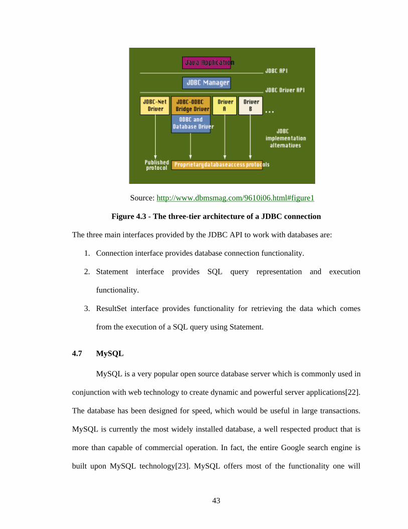
Source: http://www.dbmsmag.com/9610i06.html#figure1

Figure 4.3 - The three-tier architecture of a JDBC connection The three main interfaces provided by the JDBC API to work with databases are:

connection functionality.

2.

hich comes

4.7

conjunction with web technology server applications[22].

The database has been designed for speed, which would be useful in large transactions.

MySQL is currently the most widely installed database, a well respected product that is

more than capable of commercial operation. In fact, the entire Google search engine is

built upon MySQL technology[23]. MySQL offers most of the functionality one will

1. Connection interface provides database

Statement interface provides SQL query representation and execution

functionality.

3. ResultSet interface provides functionality for retrieving the data w

from the execution of a SQL query using Statement.

MySQL

MySQL is a very popular open source database server which is commonly used in

to create dynamic and powerful

43

expect from an RDBMS. It ensures that transactions comply with the ACID model

(Atomicity, Consistency, Isolation, and Durability), allows the building of indexes,

supports standard data types and allows for database replication, among other features.

One area where MySQL falls short is its lack of certain features like sub-queries,

constraints, views, cursors and objects. MySQL is fast, easy to use, is open source and if

the application is a web application then MySQL meshes in perfectly with most of the

web development languages. When using MySQL with java, the MySQL Connector/J

driver needs to be downloaded from MySQL’s website

[http://www.mysq

.8 Apache Tomcat

developm

application container that was created to run Servlets and Java Server Pages (JSP) in web

applications. Java m

eb pages,

servlets and JSP into a single directory structure. It can be thought of as a container

h a deployment directory where you can place all your web application files

for them

l.com/products/connector/j/].

4

Apache Tomcat (also codenamed Catalina) is a standalone Web server used as a

ent server on your desktop. The Tomcat server [21] is a java based web

ust be installed for Tomcat to operate.

Tomcat organizes all the parts of a web application such as static w

whic cts as the

to execute without any hassles.

The root folder is the deployment folder where all the static html files and JSPs

can be placed. The Servlets are placed in the ROOT/WEB-INF/Classes folder. Pros of

Tomcat are that it is an open source project, stays on top of the Servlet API

developments, and works extremely well. The cons are that it is not the fastest

implementation and that you are on your own for support.

44

In the next chapter, a detailed discussion on the developed microarray data

analysis tool is presented. The discussion is in the form of objectives of the analysis tool

and the results that have been achieved along with screen shots of the system for easier

understanding.

45

5. OBJECTIVES AND RESULTS

The aim of this thesis was to develop a freely available, platform independent

plication for visualization, normalization and analysis of microarray experiments and

so a tool which will guide the users through the steps of normalization and data analysis

such as identifying differentially expressed genes and to cluster those differentially

expressed genes into clusters of genes exhibiting similar behavior.

R, the statistical package which is freely available can be used to perform all

types of analysis on microarray data, but it has the disadvantage of being a command line

based package which requires the biologists to know the syntax of various commands and

also requires the users to be familiar with programming techniques and concepts. The

users have to in short, be well versed in R to perform efficient data analysis. Thus the

motivation for the tool comes from the need for a easy to use, point and click kind of

interface which is easily accessible over the internet, to which users can easily connect to,

upload their data files retailored to a particular format and get both numeric and visual

results for interpreting the data without having to worry about the intricacies of

programming.

I will now discuss about the different objectives of the tool and the way they were

implemented and also discuss the results of normalizing and analyzing the microarray

data using the software tool, which was developed during the course of this work.

ap

al

46

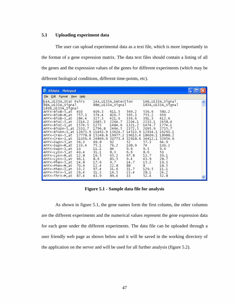
5.1 Uploading experiment data

The user can upload experimental data as a text file, which is more importantly in

the format of a gene expression m

the genes and the expression values of the genes for different experiments (which may be

different biological conditions, different time-points, etc).

atrix. The data text files should contain a listing of all

Figure 5.1 - Sample data file for analysis

As shown in figure 5.1, the gene names form the first column, the other columns

are the different experiments and the numerical values represent the gene expression data

for each gene under the different experiments. The data file can be uploaded through a

user friendly web page as shown below and it will be saved in the working directory of

the application on the server and will be used for all further analysis (figure 5.2).

47

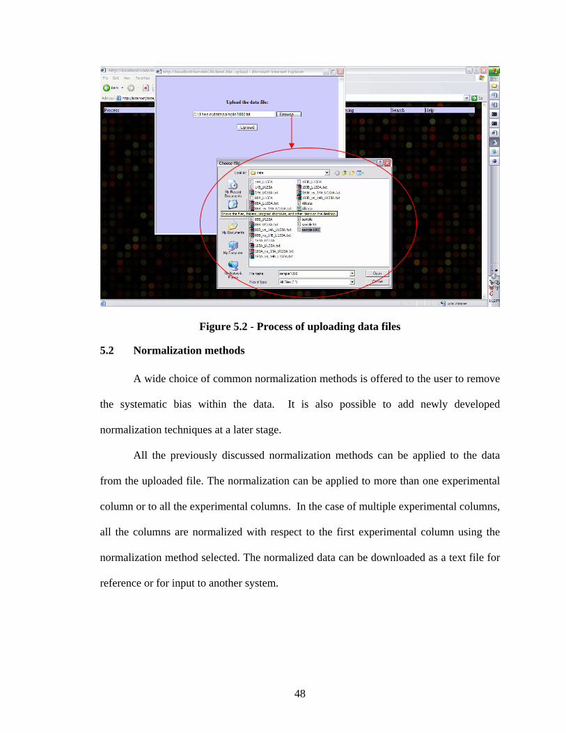
Figure 5.2 - Process of uploading data files

5.2 Normalization methods

A wide choice of common normalization methods is offered to the user to remove

the systematic bias within the data. It is also possible to add newly developed

normalization techniques at a later stage.

All the previou e applied to the data

from the uploaded file. The normalization can be applied to more than one experimental

column or to all the experimental columns. In the case of multiple experimental columns,

all the columns are normalized with respect to the first experimental column using the

normalization method selected. The normalized data can be downloaded as a text file for

reference or for input to another system.

sly discussed normalization methods can b

48

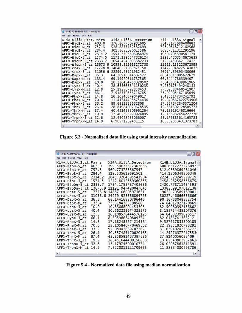
Figure 5.3 - rmalization Normalized data file using total intensity no

Figure 5.4 - Normalized data file using median normalization

49

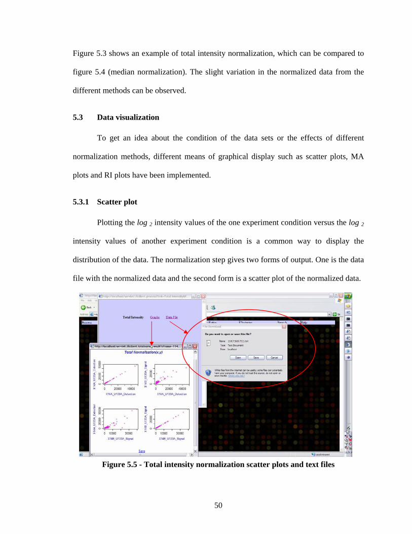
50

Figure 5.3 shows an example of total intensity normalization, which can be compared to

figure 5.4 (median normalization). The slight variation in the normalized data from the

different methods can be observed.

5.3 Data visualization

To get an idea about the condition of the data sets or the effects of different

normalization methods, different means of graphical display such as scatter plots, MA

plots and RI plots have been implemented.

5.3.1 Scatter plot

Plotting the log 2 intensity values of the one experiment condition versus the log 2

intensity values of another experiment condition is a common way to display the

distribution of the data. The normalization step gives two forms of output. One is the data

file with the normalized data and the second form is a scatter plot of the normalized data.

Figure 5.5 - Total intensity normalization scatter plots and text files

The graphical result of the normalization step is a nn× matrix of scatter plots

where n is the number of experimental columns to be normalized (figure 5.5 and 5.6).

The nn× matrix of scatter plots consists of scatte ent versus itself

and all the other experiments selected. Thus it can be observe om the results that the

scatter plot of an experiment versus itself is a straight line passing through the origin. The

matrix of the scatter plots has an image area map defined on it which lets users to

zoom in on a particular scatter plot for better viewing of the plots.

r plots of each experim

d fr

nn×

51

Figure 5.6 - matrix of scatter plots with a zoomed out portion for two specific

xperiments

MA plot

An alternative to the scatter plot is the MA plot with transformed axes to provide

intensity information. This tool produces MA plots for both normalized and raw data.

The MA plots are also produced as a

nn×

e

5.3.2

nn× matrix of individual MA plots where n is the

51

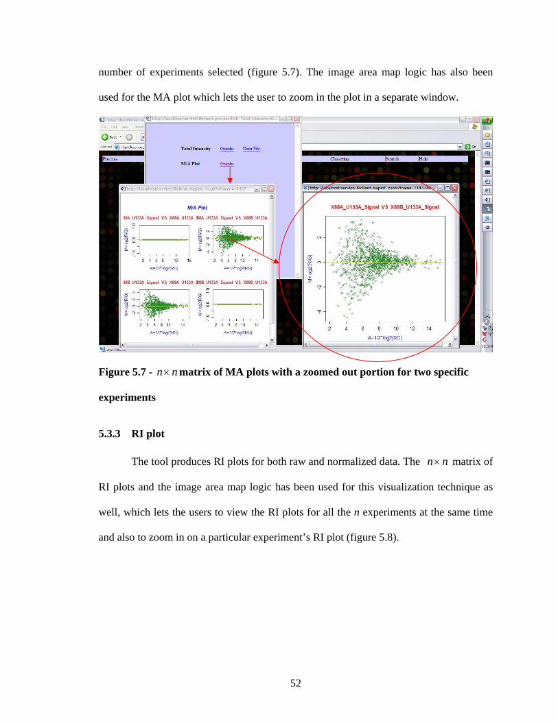
number of experiments selected (figure 5.7). The image area map logic has also been

used for the MA plot which lets the user to zoom in the plot in a separate window.

Figure 5.7 - matrix of MA plots with a z

experiments

5.3.3 RI plot

The tool produces RI plots for both raw and normalized data. The matrix of

RI plots and the image area map logic has been used for this visualization technique as

well, which lets the users to view the RI plots for all the n experiments at the same time

and also to zoom in on a particular experiment’s RI plot (figure 5.8).

nn× oomed out portion for two specific

nn×

52

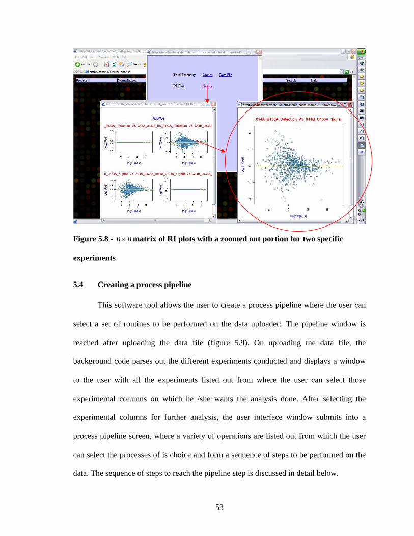
Figure 5.8 - matrix of RI plots wi

experiments

5.4 Creating a process pipeline

This software tool allows the user to create a process pipeline where the user can

a outines to be performed on the data uploaded. The pipeline window is

reached data

After selecting the

experimental columns for further analysis, the user interface window submits into a

process pipeline screen, where a variety of operations are listed out from which the user

can select the processes of is choice and form a sequence of steps to be performed on the

data. The sequence of steps to reach the pipeline step is discussed in detail below.

nn× th a zoomed out portion for two specific

select set of r

after uploading the data file (figure 5.9). On uploading the file, the

background code parses out the different experiments conducted and displays a window

to the user with all the experiments listed out from where the user can select those

experimental columns on which he /she wants the analysis done.

53

Figure 5.9 - Steps for pipelining analysis

The columns parsed out from the uploaded file, which represent the different experimental columns.

The columns transferred

double right arrow button, will be subjected to

here by clicking on the

further analysis routines.On clicking the Submit button, the window which lets the user select a pipeline of processes to be performed on the data uploaded, will open up.

Form

54

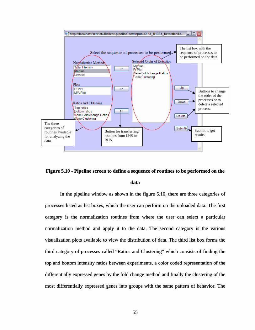
igu

rocesses listed as list boxes, which the user can perform on the uploaded data. The first

ategory is the normalization routines from where the user can select a particular

ormalization method and apply it to the data. The second category is the various

isualization plots available to view the distribution of data. The third list box forms the

ird category of processes called “Ratios and Clustering” which consists of finding the

p and bottom intensity ratios between experiments, a color coded representation of the

differentially expressed y the clustering of the

ost differentially expressed genes into groups with the same pattern of behavior. The

igure 5.10 - Pipeline screen to define a sequence of routines to be performed on the

data

In the pipeline window as shown in the figure 5.10, there are three categories of

rocesses listed as list boxes, which the user can perform on the uploaded data. The first

ategory is the normalization routines from where the user can select a particular

ormalization method and apply it to the data. The second category is the various

isualization plots available to view the distribution of data. The third list box forms the

ird category of processes called “Ratios and Clustering” which consists of finding the

p and bottom intensity ratios between experiments, a color coded representation of the

differentially expressed y the clustering of the

ost differentially expressed genes into groups with the same pattern of behavior. The

FF re 5.10 - Pipeline screen to define a sequence of routines to be performed on the

data

In the pipeline window as shown in the figure 5.10, there are three categories of

pp

cc

nn

vv

thth

toto

genes by the fold change method and finall genes by the fold change method and finall

mm

Thca

The list box with the sequence of processes to be performed on the data.

Buttons to change the order of the processes or to delete a selected process.

e three tegories of

routines available r analyzing the

data fo

Submit to get results.

Button for transferring routines from LHS to RHS.

55

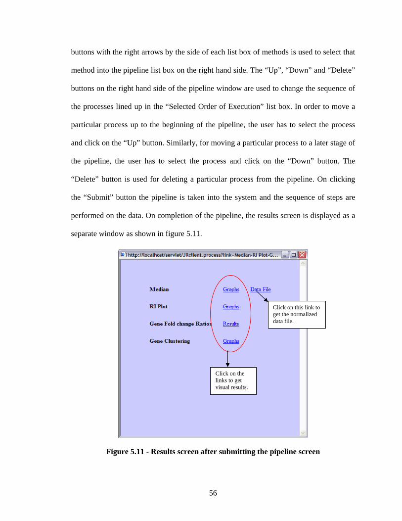
buttons with the right arrows by the side of each list box of methods is used to select that

ethod into the pipeline list box on the right hand side. The “Up”, “Down” and “Delete”

uttons on the right hand side of the pipeline window are used to change the sequence of

e processes lined up in the “Selected Order of Execution” list box. In order to move a

articular process up to the beginning of the pipeline, the user has to select the process

nd click on the “Up” button. Similarly, for moving a particular process to a later stage of

e pipeline, the user has to select the process and click on the “Down” button. The

Delete” button is used for deleting a particular process from the pipeline. On clicking

the “Submit” button the pipeline is taken into the system and the sequence of steps are

performed on the data. On completion of the pipeline, the results screen is displayed as a

parate window as shown in figure 5.11.

m

b

th

p

a

th

“

se

Figure 5.11 - Results screen after submitting the pipeline screen

Click on this link to

data file. get the normalized

Click on the links to get visual results.

56

5.5 Identifying genes of interest

One of the most important goals of microarray technology is the search for new

target genes. Methods have been provided to detect differentially expressed (DE) genes.

The techniques implemented in these methods are fold change detection and statistical t-

test.

A certain threshold value is set with which the log

5.5.1 Fold change cut-off

ous colors are assigned to represent the genes

log intensity ratio values.

2 values of the intensity ratios

of a gene between different experiments, are compared. If a gene’s log 2 intensity ratio

value exceeds the threshold value it is marked as differentially expressed (DE) in that

given experiment. In this software tool, vari

based on the gene’s 2

Cutoff Range Color coding in RGB(red, green, blue) Color image< -2.0 (153, 0, 0)

5.12 −<−≥ and (255, 0, 0) 0.15.1 −<−≥ and (255, 51, 0) 7.00.1 −<−≥ and (255, 103, 0) 5.07.0 −<−≥ and (255, 204, 51) 3.05.0 −<−≥ and (255, 204, 102) 1.03.0 −<−≥ and (255, 255, 204)

0.01.0 <−≥ and (255, 255, 230) 1.00.0 <≥ and (235, 255, 230) 3.01.0 <≥ and (204, 255, 153) 5.03.0 <≥ and (153, 255, 0) 7.05.0 <≥ and (10 , 255, 0) 3 0.17.0 <≥ and (51, 255, 0) 5.10.1 <≥ and (51, 204, 0) 0.25.1 <≥ and (0, 153, 0)

0.2≥ (0, 51, 0)

Table 5.1 - Color coding scheme for differentially expressed genes using fold change

57

The ignment of a color was done foass r easier interpretation of data. The different ranges

of the

The process of assigning colors to the different genes for a given experiment is as

follows. The intensity ratios of all the genes between the two experiments the user has

log 2 values of the intensity ratios are then calculated. The

log 2 v

provided as a tool tip (figure 5.12). On

clicking a r b tensity

ratios of the gene in other experiments and f the gene’s expressio value in all

the experiments can be vie ed (figure 5.1

log 2 intensity ratio values and the corresponding color coding assigned is given

below.

selected are calculated. The

alues are then compared with the ranges in Table 5.1. to determine a range and

then a corresponding color is assigned to the gene, thus categorizing it as either regularly

expressed, under expressed or over expressed. All the genes are plotted as matrix of

color images, where when a user does a mouse over on a particular color image, the gene

corresponding to it and the intensity value is

particular colo ox, a window opens up where the gene name, the in

a line plot o n

w 3).

58

Figure 5.12 - Color based image map of the gene’s intensity ratios between two

experiments

Figure 5.13 – Individual gene details

59

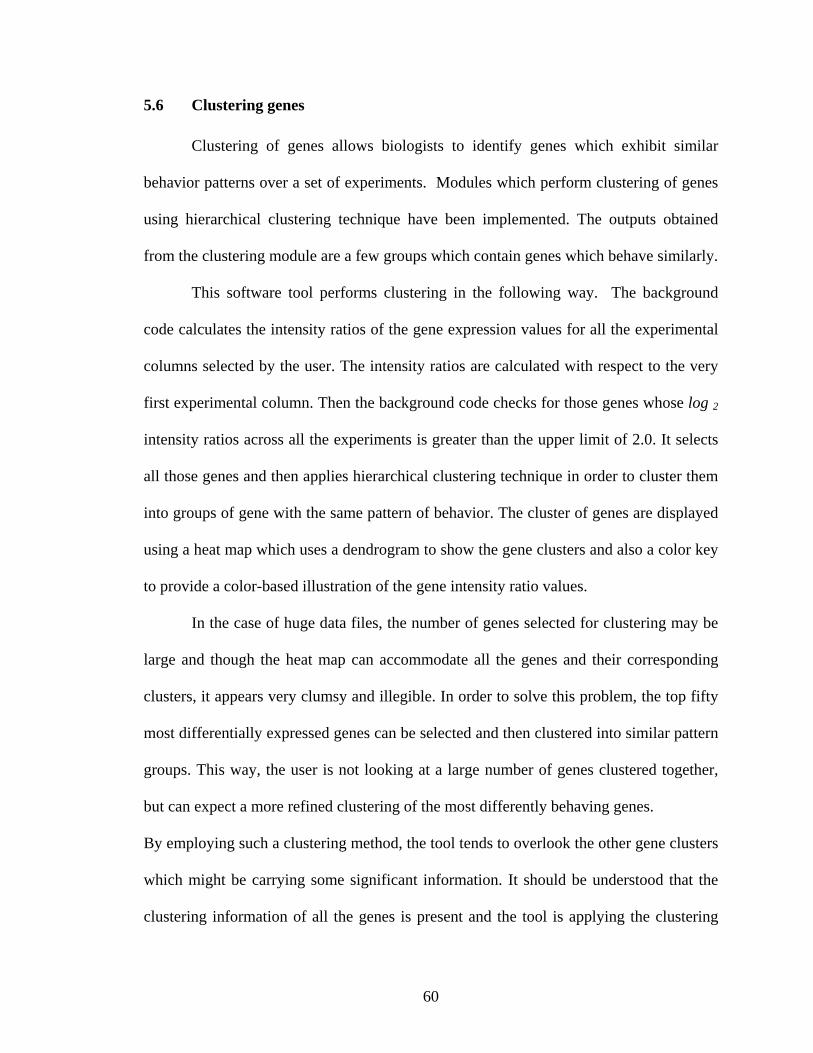
60

5.6 Clustering genes

Clustering of genes allows biologists to identify genes which exhibit similar

behavior patterns over a set of experiments. Modules which perform clustering of genes

using hierarchical clustering technique have been implemented. The outputs obtained

from the clustering module are a few groups which contain genes which behave similarly.

This software tool performs clustering in the following way. The background

code calculates the intensity ratios of the gene expression values for all the experimental

columns selected by the user. The intensity ratios are calculated with respect to the very

first experimental column. Then the background code checks for those genes whose log 2

intensity ratios across all the experiments is greater than the upper limit of 2.0. It selects

all m

into groups of gene with the same pat r. The cluster of genes are displayed

sing a heat map which uses a dendrogram to show the gene clusters and also a color key

e a color-based illustration of the gene in

In the case of huge data file

ough the heat map can accommodate all the genes and their corresponding

lusters, it appears very clumsy and illegible. In order to solve this problem, the top fifty

ected and then clustered into similar pattern

er is not looking at a large number of genes clustered together,

ut can expect a more refined clustering of the most differently behaving genes.

mploying such a clustering method, the tool tends to overlook the other gene clusters

which might be carrying be understood that the

clustering information of all the genes is present and the tool is applying the clustering

those genes and then applies hierarchical clustering technique in order to cluster the

tern of behavio

u

to provid tensity ratio values.

s, the number of genes selected for clustering may be

large and th

c

most differentially expressed genes can be sel

groups. This way, the us

b

By e

some significant information. It should

routi to all the genes anne d not just the top fifty genes. But the number of genes used for

displaying the clustered information are the ones which are most differentially expressed

in order to make the heat map (Figure 5.14) easier to view and understand.

Figure 5.14 - Heat map with a dendrogram to represent expression clusters

5.7

2

Top and bottom intensity ratios

The tool has two methods implemented for finding the top and bottom 10, 25, 50,

75 and 100 genes based on their log intensity ratios between different experiments. The

user can select the experiments for which the ratio has to be calculated for and also select

the number of top/bottom ratios needed which can be either of 10, 25, 50, 75 and 100.

Both these methods return a ordered list of genes and their intensity ratio values. The

purpose of these two methods is to provide a quick way to determine those genes which

are the most over/under expressed in a set of selected experiments.

61

or calculating the intensity ratios and the F ure 5.15 - User selected columns fig

number of top/bottom genes needed

The result screens obtained for the selections done in figure 5.15 are shown in figure

5.16. The results are displayed in the form of a table with the gene name and its

log 2 intensity ratio value.

62

Figure 5.16 - Results showing top 10 ratios and bottom 25 ratios between two

experiments

5.8

A module has bee m thousands of rows of

different

he search also returns the results of a t-test on the gene

expression profile which consists of the confidence interval for a regular gene expression

value and also the up and down regulated gene expression values based on the confidence

interval.

Search genes

n implemented for searching genes fro

gene expression information (figure 5.17). The search is done by the gene name and

returns as output, a line plot showing the behavior of the gene expression for the

experimental conditions. T

63

Figure 5.17 - Search screen with the list of genes from the uploaded data file

n intelligent one which does not require the user to scroll through

thousan

The search is a

ds of rows of gene names. Keying in the first few letters of the gene name will

highlight the gene in the displayed list. On submitting the above servlet by clicking on the

“View Graph” button, the user can view in a new window, a line plot of the gene

expression values for all the experiments in the data file, and a color coded representation

of the results of a t-test on the gene’s expression profile. The resulting screen is shown in

figure 5.18.

64

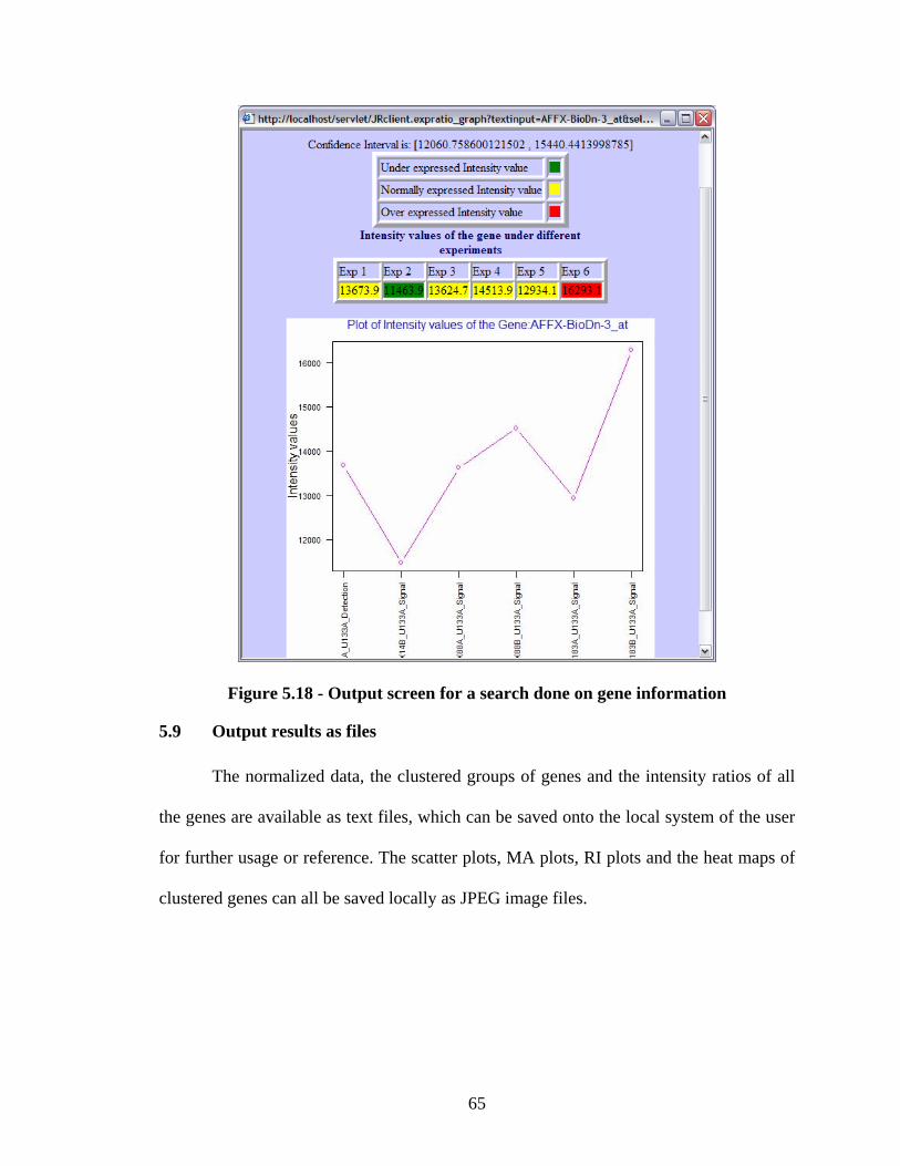
Figure 5.18 - Output screen for a search done on gene information

5.9 Output results as files

The normalized data, the clustered groups of genes and the intensity ratios of all

the genes are available as text files, which can be saved onto the local system of the user

for further usage or reference. The scatter plots, MA plots, RI plots and the heat maps of

clustered genes can all be saved locally as JPEG image files.

65

The above discussion of the results and features of the microarray data analysis

tool, show that it is a tool which will be intuitive for all the users who have a basic

understanding of normalization and data analysis. It will be a very handy tool for all

kinds of users- biologists and software developers, mainly. It’s simple user interface and

easily accessible results, supported by a help manual will help the analysis of microarray

data a simpler and easier task.

In the next chapter, some of the potential improvements that can be added to the

tool are discussed as well as the conclusions reached about optimal usage of the tool.

66

6. CONCLUSIONS

In this thesis, a platform-independent and versatile software tool for normalizing

and analyzing microarray data was developed. The software meets the requirements that

were o

ion.

The web-based front end is accessible from any web browser and handles all user

interaction. The program with its current functionality can be used by biologists for data

analysis, but there are certain improvements still in progress.

he presented program handles a wide range of functions as listed below:

• Since normalization of data is an important concern, the software tool provides

different means of normalizing the data. The possibilities are total intensity

normalization, median normalization and lowess normalization.

• The effects of normalization can be observed by useful graphical plots like scatter

plots, MA plots and RI plots. All plots can be created before and after

normalization.

• The system provides the capability of creating a pipeline of processes to be

performed on the microarray data. The user can also subject the data to specific

individual analysis techniques incase he/she does not want to create a pipeline.

riginally set forth for a tool of this nature. The interface is user-friendly. The

system is available for access to multiple users simultaneously upon user authenticat

T

67

• To detect differentially expressed genes, this tool provides simple fold-change

detection and also statistical tests like t-test. The detected target genes can be

printed to a file, for further analysis.

• Clustering methods ar sis and are also useful for reducing

6.1 Possible improvements

As with most of the software tools, this tool has a lot of scope for improvement.

Since currently new methods for normalization and analysis are developed, it may be

useful to adapt the present system to theses needs.

Possible improvements would be:

• Further normalization methods

• Additional diagnostic plots (QQ-plot, volcano plots)

•

• ent

•

tool. As far as issues are concerned, most of them have been solved and some are still in

progress.

e widely used for analy

the amount of microarray data to a subset of genes, usually to those which are

most variable between different experimental samples. This has been achieved by

using hierarchical clustering method.

• The system is expandable for further development.

ANOVA

User managem

• More sophisticated methods for detection of differentially expressed genes

Compatibility with multiple types of input data files

Many suggestions for improvement have been provided by potential users of the

68

In conclusion, this microarray data analysis tool developed using Java and R is a

nity driven solution developed to help make the analysis of microarray data

and efficient. Additional functiona

commu

simpler lity will be added on with the continuing

dev p

elo ment by other members of the Bioinformatics Research Group (BRG).

69

REFERENCES

[1] International Human Genome Sequencing Consortium, "Finishing the uchromatic sequence of the human genome," Nature, vol. 431, pp. 931-945,

[2] Tom A.van de Goor, "A History of DNA Microarrays," Advanstar ommunications Inc., 2005.

[3] eter Dalgaard, Introductory Statistics with R Springer, 2002.

[4] ff Augen, "Bioinformatics and Transcription," in Bioinformatics in the Post-Genomic Era: Genome, Transcriptome, Proteome, and Information-Based

edicine Addison Wesley Professional, 2004.

[5] .Crick, "Central dogma of molecular biology," Nature, vol. 227, no. 5258

[6] . Ruvkun, "Molecular biology.Glimpses of a tiny RNA world," Science, vol. 94, no. 5543, pp. 797-799, Aug.2001.

[7] an Cray, "Gene Detective," 2001.

[8] i Pasanen, Janna Saarela, Ilana Saarikko, Teemu Toivanen, Martti Tolvanen, auno Vihinen, and Garry Wong, DNA Microarray Data Analysis Picaset Oy,

[9] Dov Stekel, Microarray Bioinformatics Cambridge University Press, 2003.

[10] Helen C.Causton, John Quackenbush, and Alvis Brazma, A beginner's guide. icroarray Gene expression data analysis Blackwell Publishing, 2003.

[11] ordon K.Amyth, Yee Hwa Yang, and Terry Speed, "Statistical issues in cDNA Microarray Data Analysis," Functional Genomics:Methods and Protocols, vol.

24, no. Methods in Molecular Biology, pp. 111-136, 2003.

[12] hn Quackenbush, "Microarray data normalization and transformation," nature genetics supplement, vol. 32, no. December 2002, pp. 496-501, 2002.

[13] Knudsen, Guide to Analysis of DNA Microarray Data, Second ed John iley & Sons, 2004.

eOct.2004.

C

P

Je

M

FAug.1970.

G2

D

TomM2003.

M

G

2

Jo

Steen W

70

[14] W.N.Venables, D.M.Smith, and R Development Core Team, An Introduction to R Network Theory Ltd, 2004.

[15] Robert C.Gentleman, Wolfgang Huber, Vincent Carey, Rafael Irizarry, and Sandrine Dudoit, Bioinformatics and Computational Biology Solutions Using R and Bioconductor (Statistics for Biology and Health Series) Springer, 2005.

[ Source rch

[ an online 306

vsner, "SNOMAD .

[19] ide R Functionality to

[20] gan, Java in a Nutshell O'Reilly & Associates, Inc., 1997.

pache Sams Publishing, 2003.

[

16] Sandrine Dudoit, Robert C.Gentleman, and John Quackenbush, "Open Software for the Analysis of Microarray Data," Biotechniques, vol. 34, no. Ma2003, p. s45-s51, 2003.

17] Xiaoqin Xia, Michael McClelland, and Yipeng Wang, "WebArray: platform for microarray data analysis," BMC Bioinformatics, vol. 6:Dec.2005.

[18] Carlo Colantouni, George Henry, Scott Zeger, and Jonathan Pe(Standardization and NOrmalization of MicroArray Data): web-accessible geneexpression data analysis," Bioinformatics, vol. 18, no. 11, pp. 1540-1541, 2002

Simon Urbanek, "Rserve -- A Fast Way to ProvApplications," 2003.

David Flana

[21] Bruce W.Perry, Java Servlet & JSP Cookbook O'Reilly Media Inc, 2004.

[22] Julie C.Meloni, PHP, MySQL and A

23] Robert McMillan, "Loosen the reins, says Google CEO,", 11 ed 2005.

71

GLOSSARY ANOVA (Analysis Of Variance) is a collection of statistical models and their

associated procedures which compare means by splitting the overall

cDNA mplementary DNA) DNA synthesized from mRNA or DNA by

Chromosomes

the form of one or more large macromolecules called

several

exually

ome, one from

CRAN (Comprehensive R Archive Network). A network of ftp and web servers

around the world that store identical, up-to-date versions of code and

documentation for R.

DNA (Deoxyribonucleic Acid) is a nucleic acid, usually in the form of a

double helix that contains the genetic instructions specifying the

biological development of all cellular forms of life, and most viruses.

Exons The coding regions of DNA.

observed variance into different parts.

(Co

reverse transcriptase often synthesized from a cellular extract.

The DNA which carries genetic information in cells is normally

packaged in

chromosomes. Most multicellular organisms have

chromosomes, which together comprise the genome. S

reproducing organisms have two copies of each chromos

each parent.

72

Fold change The ratio of gene expression between two samples in a microarray

experiment.

Gene Units of heredity in living organisms. They are encoded in the

organism’s genetic material (usually DNA or RNA), and control the

physical development and behavior of the organism.

Genome The whole hereditary information of an organism encoded in the

DNA. It includes both genes and non-coding sequences.

Human Genome Project

A project initiated by the government of United States for DNA

sequencing of the human genome.

Hybridization The process of combining complementary, single stranded nucleic

acids into a single molecule. Nucleotides will bind to their

complement under normal conditions, so two perfectly

complementary strands will bind to each other readily.

IDE (Integrated Development Environment). Environment used for

developing code for any application.

A list of coordinates relating to a specific image, created in order to

hyperlink areas of the image to various destinations (as opposed to a

age links to a

single destination).

Introns Non-coding regions of DNA.

Java API (Java Application Programming Interface). Collection of ready-made

software components that provide several capabilities.

JDBC (Java Database Connectivity). Set of communication protocols

Image map

normal image link, in which the entire area of the im

73

between a java program and a database.

(Joint PhotogJPEG raphic Experts Group) is a commonly used standard

JSP gy which mixes

JVM programs to

JVM ter and runtime system, which lets

LAMP

LocusLink rmation about

Microarray spots attached to a physical

Microarray experiment

ing gene expression in a system under controlled

time, stimulus, developmental stage, or

MIDAS TM4 suite.

method of lossy compression for photographic images. The file

extensions for this format are .jpeg or .jpg.

(Java Server Pages). A java programming technolo

static HTML with dynamically-generated HTML.

(Java Virtual Machine). The interpreter which lets java

run on any platform where it has already been installed.

(Java Virtual Machine). An interpre

java programs run on any platform it has been ported to.

(Linux + Apache + MySQL + Python). A platform used by the

microarray data analysis tool, WebArray.

Single query interface to sequence and descriptive info

genetic loci.

A collection of microscopic DNA

substrate such as glass, plastic or silicon chip forming an array.

Microarrays are hybridized with labeled samples and then scanned

and analyzed to generate data.

An experiment study

conditions to factors such as

dosage on a sample.

(Microarray Data Analysis System). Forms a part of the

A java application which provides users an intuitive interface to

74

design analysis processes combining one or more normalization and

miRNA

pression of other genes.

A

nthesis to undergo

which a gene

MySQL

zation

riation from the microarray

Oligo tide) Short sequence of nucleotides (<80 base pairs)

Protein

gical functions of all living cells and

PubMed

from MEDLINE and other life science journals

RNA

filtering steps.

(micro RNA) is a form of single-stranded RNA which is 20-25

nucleotides long and which regulates the ex

mRN (messenger RNA) is RNA that encodes and carries information from

DNA during transcription to sites of protein sy

translation in order to yield a gene product. The amount of any

particular type of mRNA in a cell reflects the extent to

has been “expressed”.

A very popular open source database server.

Normali The process used to standardize microarray data by removing the

effect of all sources of non-biological va

data, making them comparable.

(Oligonucleo

always single stranded to be used as probes or spots.

A complex, high-molecular-weight, organic compound that consists

of amino acids joined by peptide bonds. Proteins perform a wide

variety of structural and biolo

viruses.

A service of the U.S. National Library of Medicine that includes over

16 million citations

for biomedical articles back to the 1950s.

(Ribonucleic acid) A class of nucleic acids that consist of nucleotides

75

containing the bases- adenine (A), guanine (G), cytosine (C), and

uracil (U). An RNA molecule is typically single-stranded and can pair

Servlet

SQL guage). A standard computer language for

Microarray Data Analysis System

Transcription from DNA into

Translation

ce a specific protein according to the rules specified by the

tRNA

tide chain at the ribosomal

with DNA, another RNA molecule, or form secondary structure by

hybridizing to itself.

Rserve Rserve is a TCP/IP server which allows other programs to use R

facilities without the need to initialize or link against R library.

Java program that runs on a web server and which is used to build

web pages.

(Structured Query Lan

accessing and manipulating databases.

TM4 A suite of analysis tools developed to handle all aspects of microarray

process. Includes four major applications, Microarray Data Manager

(MADAM), TIGR_Spotfinder,

(MIDAS), and Multiexperiment Viewer (MeV).

The process in which transfer of genetic information

RNA takes place. It is the beginning of the process that ultimately

leads to the translation of the genetic code into a protein.

The second process of protein synthesis, in which mRNA is decoded

to produ

genetic code. Translation is preceded by transcription.

A small RNA chain (approximately 75 bp in length) that transfers a

specific amino acid to a growing polypep

site of protein synthesis during translation.

76

CURRICULUM VITAE

Date of Birth 20, 1982

ce of Birth

Undergraduate India

Graduate Study

ter Science

Experience

uisville, KY

VASUNDHARA AKKINENI

May

Pla Madras, India

Study University of Madras, Madras,

B.Tech. Information Technology

(1999-2003)

University of Louisville, Louisville, Kentucky

M.S. Computer Engineering and Compu

(2003-2006)

IT Digitization Intern, GE Energy, Atlanta, GA

(Jan, 2005 - July, 2005)

QA Analyst Intern, Yum! Brands Inc, Louisville, KY

(June, 2004 – Dec, 2004)

Student Assistant, University of Louisville, Lo

(Aug, 2003 – May, 2004)

77