managing the soil water balance of hot pepper (capsicum annuum

Managing the soil water balance of hot pepper (Capsicum annuum

L.) to improve water productivity

by

Yibekal Alemayehu Abebe

Submitted in partial fulfilment of the requirements for the degree

Doctor of Philosophy in Horticultural Science

Department of Plant Production and Soil Science

In the Faculty of Natural and Agricultural Sciences

University of Pretoria

Pretoria

December 2009

Supervisor: Prof. J.M. Steyn

Co-supervisor: Prof. J.G. Annandale

©© UUnniivveerrssiittyy ooff PPrreettoorriiaa

ii

DECLARATION

I, Yibekal Alemayehu Abebe declare that the thesis, which I hereby submit for the degree

Doctor of Philosophy in Horticultural Science at the University of Pretoria, is my own

work and has not previously been submitted by me for a degree at this or any other

tertiary institution.

SIGNATURE: _____________________

DATE: _____________________

iii

DEDICATION

“This work is dedicated to my late father Alemayehu Abebe Kenne who inspired me to

pursue higher learning and my wife Alem Sinshaw Belay and my son Abel Yibekal

Alemayehu who sacrificed much due to my long absence.”

iv

PREFACE

This PhD thesis was prepared in the Department of Plant Production and Soil Science at

the University of Pretoria, South Africa. The project involved two field trials, a rain-

shelter trial and growth cabinet experiments at the Hatfield Experimental Farm,

University of Pretoria. Data on soil and climate from five agro-ecological regions of

Ethiopia were also used in the project. The main aim of this work was to assess

management options and modelling approaches to designing management strategies to

increase the water-use efficiency of hot pepper.

In Chapter 1, a brief introduction on hot pepper origin, ecology, deficit irrigation and

irrigation scheduling was given. It also highlights the importance of careful selection of

cultivars and plant populations for maximizing yield and the water-use efficiency (where

water is limiting) of hot pepper. In Chapter 2, an elaborate literature review of the

importance of water in plant production, and biological, agronomic, management and

engineering means of improving water productivity in crop production were conducted.

A detailed literature review was also done on the effects of different irrigation regimes on

crop production in general and hot pepper production in particular. The role of varying

plant populations on yield and quality of hot pepper was also reviewed.

In Chapter 3, effects of varying irrigation regimes on yield and water-use efficiency of

hot pepper were investigated. In general, results from this study show that hot pepper is a

water stress sensitive plant and frequent irrigation is crucial for optimum yield. The

results also suggest that increasing the water-use efficiency by decreasing water

application seems unattainable, as yield reduction is remarkably high due to decreased

water supply.

In Chapter 4, effects of row spacing on yield and water-use efficiency of hot pepper were

investigated. Generally, narrow row spacing significantly increased both yield and water-

use efficiency of hot peppers. In Chapter 5, the combined effects of irrigation regimes

and row spacing on yield and water-use efficiency of hot pepper were investigated. The

results show that both high water supply and narrow row spacing increase yield. The

water-use efficiency was also improved by narrow row spacing.

v

In Chapter 6, the agronomic and climatic data from the field experiments are utilized to

determine FAO-type crop factors. This information is useful to schedule irrigation using

the Soil Water Balance (SWB) and/or CROPWAT irrigation scheduling models.

Similarly, in Chapter 7, field and climatic data collected are used to determine crop-

specific growth model parameters for five hot pepper cultivars. This information is

important to schedule irrigation using the SWB crop growth and other growth models. In

both Chapters 6 and 7, attempts are made to create guidelines that help to estimate crop-

specific model parameters from morphological features and maturity groupings of other

hot pepper cultivars not included in this study.

In Chapter 8, attempts are made to determine cardinal temperatures: base, optimum, and

cut-off temperatures for two hot pepper cultivars in studies conducted in the growth

cabinet. It was very clear that cardinal temperatures for hot pepper cultivars in the

vegetative and reproductive stages are markedly different.

In Chapter 9, the SWB model is calibrated and evaluated. The results show that most of

the crop growth parameters considered was successfully simulated. The soil water deficit

to field capacity was also simulated with sufficient accuracy to schedule irrigations. In

Chapter 10, soil and climate data from five agro-ecological regions of Ethiopia are

utilized to develop irrigation calendars and estimate water requirements of hot pepper

cultivar Mareko Fana. Air temperatures, average wind speed and solar radiation appeared

to influence the irrigation frequency, depth of irrigation and total water requirements.

In chapter 11, general conclusions and recommendations are provided. Furthermore,

future research needs that have emanated from the present work are identified.

Four hot pepper cultivars (Jalapeno, Long Slim, Malaga, and Serrano) from South Africa

and one (Mareko Fana) from Ethiopia were used in the study. The selection criteria used

for the inclusion of these cultivars in this study were the diversity in terms of growth and

fruit types they offered and their commercial importance.

The thesis is presented in article format. One article is published, while others were

prepared for publication. The thesis is prepared in accordance with the guidelines for

authors for the publication of manuscripts in the South African Journal of Plant and Soil.

vi

ALEMAYEHU, Y.A., STEYN, J.M. & ANNANDALE, J.G., 2009. FAO-type crop

factor determination for irrigation scheduling of hot pepper (Capsicum annuum

L.) cultivars. S. Afr. J. Plant Soil. 26 (3), 186-194.

ALEMAYEHU, Y.A., STEYN, J.M. & ANNANDALE, J.G., 2009. SWB parameter

determination and stability analysis under different irrigation regimes and row

spacings of hot pepper (Capsicum annuum L) cultivars. (Prepared to be submitted

for publication in the South African Journal of Plant and Soil).

ALEMAYEHU, Y.A., STEYN, J.M. & ANNANDALE, J.G., 2009. Calibration and

validation of the SWB irrigation scheduling model for hot pepper (Capsicum

annuum L.) cultivars for contrasting plant populations and soil water regimes.

(Prepared to be submitted for publication in the South African Journal of Plant

and Soil).

ALEMAYEHU, Y.A., STEYN, J.M. & ANNANDALE, J.G., 2009. Yield and water-use

efficiency of hot pepper (Capsicum annuum L) as affected by irrigation regime

and row spacing. (Prepared to be submitted to New Zealand Journal of Crop and

Horticultural Science).

ALEMAYEHU, Y.A., STEYN, J.M. & ANNANDALE, J.G., 2009. Irrigation calendars

and water requirements of hot pepper cultivar Mareko Fana in five agro-

ecological regions of Ethiopia. (Prepared to be submitted for publication in the

East African Journal of Agriculture and Sciences).

vii

ACKNOWLEDGEMENTS

I would like to extend my deepest gratitude and thanks to my supervisors, Prof. J.M.

Steyn and Prof. J.G. Annandale, for their encouragement, support, guidance, and

constructive comments throughout the course of the studies. I am duly grateful to my

supervisors for the financial assistance I received during the latter part of my studies.

Special thanks go to Haramaya University for sponsoring my study through the World

Bank supported Agricultural Research Training Project (ARTP). I thank all the task force

members of ARTP for their understanding and encouragement to finish this study.

I would like to acknowledge the support I received doing the experiments at the Hatfield

Experimental Farm and would like to thank all the staff working there. I am deeply

indebted to all my friends at the University of Pretoria and the Haramaya University

whose support was indispensable in executing the field work, and whose friendly

encouragement helped me to overcome the ups and downs that postgraduate studies

demand.

I remain indebted to all my family members for their prayers, unstinting support and all-

consuming love.

viii

ABSTRACT

A series of field, rainshelter, growth cabinet and modelling studies were conducted to

investigate hot pepper response to different irrigation regimes and row spacings; to

generate crop-specific model parameters; and to calibrate and validate the Soil Water

Balance (SWB) model. Soil, climate and management data of five hot pepper growing

regions of Ethiopia were identified to develop irrigation calendars and estimate water

requirements of hot pepper under different growing conditions.

High irrigation regimes increased fresh and dry fruit yield, fruit number, harvest index

and top dry matter production. Yield loss could be prevented by irrigating at 20-25%

depletion of plant available water, confirming the sensitivity of the crop to mild soil water

stress. High plant density markedly increased fresh and dry fruit yield, water-use

efficiency and dry matter production. Average fruit mass, succulence and specific leaf

area were neither affected by row spacing nor by irrigation regimes. There were marked

differences among the cultivars in fruit yields despite comparable top dry mass

production. Average dry fruit mass, fruit number per plant and succulence were

significantly affected by cultivar differences. The absence of interaction effects among

cultivar and irrigation regimes, cultivars and row spacing, and irrigation regimes and row

spacing for most parameters suggest that appropriate irrigation regimes and row spacing

that maximize productivity of hot pepper can be devised across cultivars.

To facilitate irrigation scheduling, a simple canopy cover based procedure was used to

determine FAO-type crop factors and growth periods for different growth stages of five

hot pepper cultivars. Growth analysis was done to calculate crop-specific model

parameters for the SWB model and the model was successfully calibrated and validated

for five hot pepper cultivars under different irrigation regimes or row spacings. FAO

basal crop coefficients (Kcb) and crop-specific model parameters for new hot pepper

cultivars can now be estimated from the database, using canopy characteristics, day

degrees to maturity and dry matter production.

Growth cabinet studies were used to determine cardinal temperatures, namely the base,

optimum and cut-off temperatures for various developmental stages. Hot pepper cultivars

were observed to require different cardinal temperatures for various developmental

ix

stages. Data on thermal time requirement for flowering and maturity between plants in

growth cabinet and open field experiments matched closely. Simulated water

requirements for hot pepper cultivar Mareko Fana production ranged between 517 mm at

Melkassa and 775 mm at Alemaya. The simulated irrigation interval ranged between 9

days at Alemaya and 6 days at Bako, and the average irrigation amount per irrigation

ranged between 27.9 mm at Bako and 35.0 mm at Zeway.

Key words: Basal crop coefficient, Capsicum annuum, cardinal temperature, model

parameter, hot pepper, irrigation calendar, irrigation regimes, plant density, row spacing,

Soil Water Balance model, water-use efficiency

x

TABLE OF CONTENTS

DECLARATION .......................................................................................... ii

DEDICATION ............................................................................................. iii

PREFACE .................................................................................................... iv

ACKNOWLEDGEMENTS ...................................................................... vii

ABSTRACT ...............................................................................................viii

LIST OF FIGURES ................................................................................. xvii

LIST OF TABLES ..................................................................................... xx

LIST OF SYMBOLS AND ABBREVIATIONS ..................................xxiii

CHAPTER 1

GENERAL INTRODUCTION ................................................................... 1

1.1 Botany and ecology of hot pepper ................................................................................. 1

1.2 Irrigation, irrigation scheduling and deficit irrigation ................................................... 2

1.3 Justification of the study ................................................................................................ 5

1.4 Objectives of the study ................................................................................................... 6

CHAPTER 2

LITERATURE REVIEW ........................................................................... 8

2.1 The role of water in plant production ............................................................................ 8

2.2 Water availability for crop production in semi-arid and arid regions ............................ 9

2.3 Increasing water-use efficiency ..................................................................................... 9

2.3.1 Breeding crops for improved water-use efficiency .............................................. 10

xi

2.3.2 Water-saving agriculture ...................................................................................... 12

2.3.2.1 Increasing precipitation use efficiency ............................................................ 12

2.3.2.2 Increasing water-use efficiency ....................................................................... 13

2.4 A brief description of the Soil Water Balance model .................................................. 19

2.5 Water requirements of peppers and water stress effects on peppers ........................... 20

2.6 Planting density effect on growth, yield and water-use of plants ................................ 22

CHAPTER 3

THE EFFECT OF DIFFERENT IRRIGATION REGIMES ON

GROWTH AND YIELD OF THREE HOT PEPPER (Capsicum

annuum L.) CULTIVARS ........................................................................ 25

3. 1 INTRODUCTION ....................................................................................................... 27

3.2 MATERIALS AND METHODS ................................................................................. 29

3.2.1 Experimental site and treatments ......................................................................... 29

3.2.2 Crop management ................................................................................................ 29

3.2.3 Measurements ...................................................................................................... 30

3.2.4 Data analysis ........................................................................................................ 31

3.3 RESULTS AND DISCUSSION ................................................................................. 32

3.3.1 Specific leaf area, leaf area index and canopy development ............................... 32

3.3.2 Dry matter production and distribution ................................................................ 33

3.3.3 Yield, yield components and selected quality measures ...................................... 36

3.3.4 Water-use and water-use efficiency ..................................................................... 39

3.4 CONCLUSIONS .......................................................................................................... 43

xii

CHAPTER 4

RESPONSE OF HOT PEPPER (Capsicum annuum L.) CULTIVARS

TO DIFFERENT ROW SPACINGS ....................................................... 44

4.1 INTRODUCTION ....................................................................................................... 46



4.2.2 Crop management ................................................................................................ 48

4.2.3 Measurements ...................................................................................................... 49

4.2.4 Data analysis ........................................................................................................ 50

4.3 RESULTS AND DISCUSSION .................................................................................. 51


4.3.2 Dry matter production and partitioning ............................................................... 52

4.3.3 Fruit yield, yield components and selected quality measures .............................. 55

4.3.4 Soil water content, water-use and water-use efficiency ....................................... 57

4.4. CONCLUSIONS .......................................................................................................... 59

CHAPTER 5

EFFECTS OF ROW SPACINGS AND IRRIGATION REGIMES ON

GROWTH AND YIELD OF HOT PEPPER (Capsicum annuum L. CV

‘CAYENNE LONG SLIM’) ...................................................................... 60

5.1 INTRODUCTION ....................................................................................................... 62



5.2.2 Crop management ................................................................................................ 64

xiii

5.2.3 Measurements ...................................................................................................... 65

5.2.4 Data analysis ........................................................................................................ 66



5.3.2 Dry matter production and partitioning ............................................................... 68

5.3.3 Yield, yield components and selected quality measures ...................................... 71

5.3.4 Soil water content, water-use and water-use efficiency ....................................... 73

5.4 CONCLUSIONS .......................................................................................................... 76

CHAPTER 6

FAO-TYPE CROP FACTOR DETERMINATION FOR IRRIGATION

SCHEDULING OF HOT PEPPER (Capsicum annuum L.)

CULTIVARS .............................................................................................. 77

6.1 INTRODUCTION ....................................................................................................... 78



6.2.2 Crop management and measurements ................................................................. 80

6.2.3 The Soil Water Balance (SWB) model ................................................................ 84


6.3.1 Canopy development, root depth, leaf area index and plant height ..................... 85

6.3.2 Basal crop coefficients and growth periods ......................................................... 86

6.3.3 Water-use and crop coefficients ........................................................................... 94

6.3.4 Model simulation results ...................................................................................... 96

6.4 CONCLUSIONS .......................................................................................................... 99

xiv

CHAPTER 7

SWB PARAMETER DETERMINATION AND STABILITY

ANALYSIS UNDER DIFFERENT IRRIGATION REGIMES AND

ROW SPACINGS IN HOT PEPPER (Capsicum annuum L)

CULTIVARS ............................................................................................ 100

7.1 INTRODUCTION ..................................................................................................... 102

7.2 MATERIALS AND METHODS ............................................................................... 104

7.2.1 Experimental site and treatments ………………………..………………….… 104

7.2.2 Crop management and measurements ............................................................... 104

7.2.3 Crop-specific parameter determination and data analysis ………...…………...105

7.3 RESULTS AND DISCUSSION ................................................................................ 109

7.3.1 Canopy radiation extinction coefficient for PAR (KPAR) ................................... 109

7.3.2 Radiation use efficiency (Ec) ............................................................................. 112

7.3.3 Specific leaf area and leaf-stem partitioning parameter .................................... 115

7.3.4 Vapour pressure deficit-corrected dry matter/water ratio (DWR) ……………..117

7.3.5 Thermal time requirements ................................................................................ 118

7.3.6 Crop-specific model parameters for newly released cultivars ........................... 118

7.4 CONCLUSIONS ........................................................................................................ 122

CHAPTER 8

THERMAL TIME REQUIREMENTS FOR THE DEVELOPMENT

OF HOT PEPPER (Capsicum annuum L.) ........................................... 123

8.1 INTRODUCTION ..................................................................................................... 124


xv

8.2.1 Germination study .............................................................................................. 126

8.2.2 Developmental stage experiments ..................................................................... 126

8.2.3 Field experiment ................................................................................................ 127

8.2.4 Data collection and analysis ............................................................................... 127

8.2.4.1 Cardinal temperature determination .............................................................. 127

8.2.4.2 Thermal time determination ........................................................................... 128


8.3.1 Germination ....................................................................................................... 129

8.3.2 Developmental stages ........................................................................................ 132

8.3.3 Validating results with field data ....................................................................... 136

8.4 CONCLUSIONS ........................................................................................................ 138

CHAPTER 9

CALIBRATION AND VALIDATION OF THE SWB IRRIGATION

SCHEDULING MODEL FOR HOT PEPPER (Capsicum annuum L.)

CULTIVARS FOR CONTRASTING PLANT POPULATIONS AND

IRRIGATION REGIMES ...................................................................... 139

9.1 INTRODUCTION ..................................................................................................... 140


9.2.1 Experimental site and treatments ....................................................................... 142

9.2.2 Crop management and measurements ............................................................... 142

9.2.3 The Soil Water Balance model .......................................................................... 143

9.2.4 Determination of crop-specific model parameters ............................................. 144

9.2.5 Cultivars used in calibration and validation studies .......................................... 144

xvi

9.2.6 Model reliability test .......................................................................................... 145


9.4 CONCLUSIONS......................................................................................................... 154

CHAPTER 10

PREDICTING CROP WATER REQUIREMENTS FOR HOT

PEPPER CULTIVAR MAREKO FANA AT DIFFERENT

LOCATIONS IN ETHIOPIA USING THE SOIL WATER BALANCE

MODEL .................................................................................................... 155

10.1 INTRODUCTION ..................................................................................................... 156


10.2.1 Site and procedures description ....................................................................... 159

10.2.2 The Soil Water Balance (SWB) model ............................................................ 162

10.3 RESULTS AND DISCUSSION ............................................................................ …164

10.4 CONCLUSIONS ........................................................................................................ 170

CHAPTER 11

GENERAL CONCLUSIONS AND RECOMMENDATIONS ........... 171

11.1 GENERAL CONCLUSIONS .................................................................................... 171

11.2 GENERAL RECOMMENDATIONS ....................................................................... 178

11.3 RECOMMENDATION FOR FURTHER RESEARCH .......................................... 180

LIST OF REFERENCES ........................................................................ 181

APPENDICES ………………………………….……..…...…………... 200

xvii

LIST OF FIGURES

Figure 3.1 Top (TDM), leaf (LDM) and stem (SDM) dry matter as

affected by cultivar (a) and irrigation regime (b) …………..……………34

Figure 3.2 Soil water content to 0.6 m soil depth during growing season as

influenced by irrigation regimes ……………..………………………….40

Figure 5.1 Top (TDM), leaf (LDM) and stem (SDM) dry matter as

affected by row spacings (a) and irrigation regimes (b) ……….………. 69

Figure 5.2 Soil water content to 0.6 m soil depth during the growing season

as influenced by plant density (a) and irrigation regime (b) ……….……74

Figure 6.1 Measured values of canopy cover (FI) and estimated root depth

(RD) during the growing season of hot pepper cultivar Long Slim ..........85

Figure 6.2 Daily values of canopy cover (FI daily) and basal crop coefficient

(Kcb daily), and estimated Kcb values for three growth stages of hot

pepper cultivar Long Slim under high density and high irrigation

treatment (initial, crop development and mid-season stages) ...................88

Figure 6.3 Photos of hot pepper cultivars used in the experiments. ……………...…92

Figure 6.4 Crop coefficient (Kc) calculated for hot pepper cultivar Long Slim ....…94

Figure 6.5 Measured and simulated fractional interception (FI) during the

growing season for cultivar Long Slim under high irrigation

(calibration, HI) and water stress conditions (validation, LI) .……..……97

Figure 6.6 Measured and simulated soil water deficit to field capacity (Deficit)

during the growing season for cultivar Long Slim under high

irrigation (calibration, HI) and water stress

conditions (validation, LI) ………………………...……………………..98

xviii

Figure 7.1 Regression between leaf area index (LAI) and natural logarithm

of transmitted PAR for five hot pepper cultivars under medium

(55D) irrigation and 0.70 m row sapcing …………………………….. 110

Figure 7.2 Dry matter (DM) production of five hot pepper cultivars, under

medium irrigation (55D) and 0.7 m row spacing, as a function

of the cumulative product of fractional interception

(FI) and total solar radiation (PAR) …………………………………...113

Figure 7.3 Determination of the leaf-stem dry matter partitioning parameter (p)

as a function of canopy dry matter (CDM), specific leaf area (SLA)

and leaf area index (LAI) for five hot pepper cultivars under

medium irrigation and 0.7 m row spacing ………………….………...116

Figure 8.1 Temperature response of time for 50% germination for the cultivar

Jalapeno (a), determination of the cardinal temperatures for 50%

germination for the cultivar Jalapeno (b) …………………………...…130

Figure 8.2 Thermal time requirement for 50% germination, calculated at

four constant temperatures for the cultivar Jalapeno …………….…... 131

Figure 8.3 Temperature response of time from sowing/transplanting to

Developmental stages for the cultivar Jalapeno (a) and

Mareko Fana (b) ………..................................................................…... 133

Figure 8.4 Determination of the cardinal temperatures for various developmental

stages for the cultivar Jalapeno (a) and Mareko Fana (b) ….……....….134

Figure 8.5 Comparison of growth cabinet and field thermal time requirements of

flowering and maturity for the cultivars Mareko Fana (MF) and Jalapeno

(JP) using growth cabinet determined cardinal temperatures …......…...137

Figure 9.1 Simulated (solid lines) and measured values (points) of fractional

interception (FI), leaf area index (LAI), soil water deficit (Deficit),

top dry matter (TDM) and harvestable dry matter (HDM) [Jalapeno

calibration, well irrigated] of the measurement …………...…………..148

xix


interception (FI), leaf area index (LAI), soil water deficit, top dry

matter (TDM) and harvestable dry matter (HDM) [Serrano

calibration, high density planting] …………………………..………...148



matter (TDM) and harvestable dry matter (HDM) [Long Slim

calibration, well irrigated and high density planting] ……………..…. 149


interception (FI), leaf area index (LAI), soil water deficit (Deficit),

top dry matter (TDM) and harvestable dry matter (HDM) [Jalapeno

validation, deficit irrigation] …………………………………….…....151

Figure 9.5 Simulated (solid lines) and measured values (points) of

fractional interception (FI), leaf area index (LAI), soil

water deficit, top dry matter (TDM) and harvestable dry

matter (HDM) [Serrano validation, low density planting] …………....152



matter (TDM) and harvestable dry matter (HDM) [Long Slim

validation, deficit irrigation and low density planting] ……………….153

Figure 10.1 Geographic distribution of the five ecological regions of Ethiopia

considered in the study ………………………………………………...161

Figure 10.2 Penman-Monteith grass reference daily evapotranspiration

(ETo) (a) and cumulative thermal time to maturity (b)

for Mareko Fana under five sites ……………………….……………. 166

Figure 10.3 Relationship between cumulative crop evapotranspiration and

top dry matter production of Mareko Fana for five

ecological regions of Ethiopia ……………………...………………….169

xx

LIST OF TABLES

Table 3.1 Specific leaf area (SLA), leaf area index (LAI) and fractional

interception of photosynthetically active radiation (FIPAR) as

affected by different irrigation regimes and cultivars ……………...….. 33

Table 3.2 Dry matter partitioning to fruits, leaves and stems as affected by

different irrigation regimes and cultivars ………………………..……....35

Table 3.3 Friut yield, yield components and some quality measures as

affected by different irrigation regimes and cultivars ……………....…. 37

Table 3.4 Components of soil water balance as affected by different

cultivars and irrigation regimes ………………………………………… 40

Table 3.5 Water-use efficiency as affected by differentcultivars

and irrigation regimes ………………………..........................................42


interception (FI) as affected by different row spacings and cultivars …..51

Table 4.2 Top dry matter (TDM), leaf dry matter (LDM) and stem dry

matter (SDM) as affected by different row spacings and cultivars …....53

Table 4.3 Dry matters partitioning to fruits, leaves and stems as affected by

different row spacings and cultivars ……………………………………54

Table 4.4 Fruit yield, yield components and selected quality measures as

affected by different row spacings and cultivars ………………..............56

Table 4.5 Components of soil water balance as affected by different

cultivars and row spacing ………………………………….……………58

Table 4.6 Water-use efficiency as affected by different cultivars and

row spacings ………………………………………………………....….58

xxi


Interception (FI) as affected by different row spacings and

irrigation regimes ………………………………………..………...…....68

Table 5.2 Dry matter partitioning to fruits, leaves and stems as affected by

different row spacings and irrigation regimes …………………….……70

Table 5.3 Fruit yield, yield components and selected quality measures as

affected by different row spacings and irrigation regimes ………..…….71

Table 5.4 Water-use and water-use efficiency (WUE) as affected by

different row spacings and irrigation regimes ……………….………….75

Table 6.1 Soil chemical and physical properties of experimental plots ……...….....81

Table 6.2 Treatments, experimental design and planting date of experiments ….... 81

Table 6.3 Maximum root depth (RD), maximum crop height (Hcmax), 90%

of maximum canopy cover (0.9FImax) and leaf area index (LAI)

at 0.9FImax for five hot pepper cultivars …………………....……..….....87

Table 6.4 Basal crop coefficients (Kcb), and growth period (initial, development,

mid-season and late-season stages) for five hot pepper cultivars ….….. 89

Table 6.5 Some features of the hot pepper cultivars used in the experiment ….......92

Table 6.6 Soil water storage (�S), simulated seasonal value of evaporation from

the soil surface (Esim), transpiration (Tsim) and evapotranspiration

(ETsim) and measured seasonal evapotranspiration (ETmeas)

for five hot pepper cultivars …………………………….…………..…...96

Table 7.1 Test of homogeneity of regression coefficient for canopy extinction

coefficients for PAR (KPAR) and radiation conversion efficiency

(Ec) for five hot pepper cultivars under different row spacing

and/or irrigation regimes ………………………………...……………111

Table 7.2 Leaf-stem partitioning parameter (p), specific leaf area (SLA),

vapour pressure deficit-corrected dry matter/water ratio (DWR) .….….114

xxii

Table 7.3 Specific leaf area (SLA), vapour pressure-corrected dry matter/water

ratio (DWR), day degree to 50% flowering (DDF) and maturity

(DDM) for five hot pepper cultivars under 0.7 m row spacing and

medium irrigation regimes (55D) ………………………………...…...117

Table 7.4 Some features of the hot pepper cultivars considered for the

estimation of the SWB model parameters in the experiment ……...…..121

Table 9.1 Crop-specific model parameters calculated from growth

analysis on high irrigated regime (D25) and/or high density planting

(HD) and used to calibrate SWB for different hot pepper cultivars …...146

Table 10.1 Geographical description of the stations used for the study …………..159

Table 10.2 Monthly climatic variables of the five ecological regions

of Ethiopia during the growing season ………………………….……. 159

Table 10.3 Soil physical properties for the five ecological regions of Ethiopia ..... 161

Table 10.4 Crop-specific model parameters of Mareko Fana used to run

the SWB .………………………………………………………………162

Table 10.5 Irrigation calendar output format of the SWB model ……………….…164

Table 10.6 Simulated irrigation calendar for five ecological regions of

Ethiopia for hot pepper production …………….……………………..165

Table 10.7 Simulated hot pepper soil water balance for five ecological regions of

Ethiopia under high irrigation …………………….................................168

Table 10.8 Simulated hot pepper productivity at five ecological regions of Ethiopia

under full irrigation …………………………………………...………..168

xxiii

LIST OF SYMBOLS AND ABBREVIATIONS

�S Change in soil water storage

�t Time step

°C d Day degrees Celsius

°C Degree Celsius

25D Irrigation to field capacity at 20-25% depletion of plant available water



an Leaf absorptance of near infrared radiation

ap Leaf absorptance of PAR

as Leaf absorptance of solar radiation

CAI Controlled alternative irrigation

CDM Canopy dry matter

cm Centimetre

CO2 Carbon dioxide

CV Coefficient of variation

D Drainage

d Willmott’s index of agreement

DDF Day degrees to 50% flowering

DDM Day degrees to maturity

DM Dry matter

DPAW Depletion of plant available water

DWR Vapour pressure deficit-corrected dry matter/water ratio

E East

xxiv

ea Actual vapour pressure

Ec Radiation use efficiency

Eq. Equation

es Saturated vapour pressure

Es Soil evaporation

Esim Simulated seasonal soil evaporation

EsTmax Saturated vapour pressure at maximum air temperature

EsTmin Saturated vapour pressure at minimum air temperature

ET Evapotranspiration

ETc Crop evapotranspiration

ETmeas Measured seasonal evapotranspiration

ETo FAO reference evapotranspiration

ETsim Simulated seasonal evapotranspiration

FAO Food and agriculture Organization of the United Nations

FC Field capacity

FI Fractional canopy cover

FIPAR Fractional interception for PAR

FIS Fractional interception for total solar radiation

g Gram

GDD Growing day degrees

GLM General linear model

H2O Water

ha Hectare

Hc Crop height

xxv

Hcmax Maximum crop height

HDM Harvestable dry matter

HI Harvest index

I Irrigation

K Potassium

Kbd Canopy radiation extinction coefficient for ‘black’ leaves

Kc Crop coefficients

Kcb Basal crop coefficients

Kcmax The maximum value for Kc following rain or irrigation

Ke Soil evaporation coefficient

kg Kilogram

kPa Kilopascal

KPAR Canopy radiation extinction coefficient for PAR

Ks Canopy radiation extinction coefficient for total solar radiation

l Litre

LAI Leaf area index

LDM Leaf dry matter

ln Natural logarithm

LSD Least square differences

m Meter

m.a.s.l. Meter above sea level

MAE Mean absolute error

mg Milligram

xxvi

MJ Mega joule

mm millimeter

N Nitrogen

n Number of observation

NIR Near infrared

NR Narrow row

NS Not significant

p Leaf-stem partitioning parameter

P Phosphorous

p Probability level

Pa Pascal

PAR Photosynthetically active radiation

PAW Plant available water

PE Potential evaporation

PET Potential evapotranspiration

PRD Partial root zone drying

PT Potential transpiration

PWP Permanent wilting point

R Runoff

r2 Coefficient of determination

RCBD Randomized complete block design

RDI Regulated deficit irrigation

RDmax Maximum rooting depth

RF Precipitation (rainfall)

xxvii

RHmax Daily maximum relative humidity

RHmin Daily minimum relative humidity

RMSE Root mean square error

Rs Daily total incident solar radiation

S South

SDM Stem dry matter

SE Standard errors of means

SLA Specific leaf area

SPAC Soil-plant-atmosphere continuum

SWB Soil Water Balance model

SWC Soil water content

t Ton

T Transpiration

Tamax Maximum air temperature

Tamin Minimum air temperature

Tavg Average air temperature

Tb Base temperature

TDM Top dry matter

TDMP Top dry matter production

TE Transpiration efficiency

Tm Optimum temperature for crop growth

Tmax Maximum transpiration rate

Tsim Simulated seasonal crop transpiration

Tx Cut-off temperature

xxviii

U Wind speed

U2 Mean daily wind speed at 2 m height

UN United Nations

VPD Vapour pressure deficit

WR Wide row

WUE Water-use efficiency

Y Yield

�m Micrometer

�lm Leaf water potential at maximum transpiration

1

CHAPTER 1

GENERAL INTRODUCTION

1.1 Botany and ecology of hot pepper

Hot pepper (Capsicum spp.), commonly known as chili, is the world’s third most

important vegetable after potatoes and tomatoes in terms of quantity of production. World

production of chili and pepper is 28.4 million tons both dry and green fruit from 3.3

million ha, with an annual growth rate of 0.5% (FAO, 2007). Authorities generally agree

that Capsicum originated in the new world tropics and subtropics (Mexico, Central

America, and Andes of South America) over 2000 years ago (Walter, 1986). Chili

belongs to the family Solanaceae and genus Capsicum. The genus Capsicum comprises

20-30 species (Lovelock, 1973). The species annuum, however, is the most commonly

cultivated (Smith et al., 1998).

As a food, pepper has little energy value but it is an excellent source of vitamins A and C

and a good source of vitamin B2, potassium, phosphorus, and calcium. The high nutritive

value of pepper results in a high market demand year round. Pepper fruits are used in

salads, pickles, stuffing, spices, sauce, and as a dried powder. The leaves are used in

salads, soups, or eaten with rice (Lovelock, 1973).

Hot peppers are adapted to hot weather conditions. Day temperatures of 24 to 30 °C and

night temperatures about 10 to 15 °C are ideal for growth. They are sensitive to freezing

temperatures, while temperatures above 32 °C can reduce pollination, fruit set and yield

(Smith et al., 1998). They are considered to be quantitative short day plants (Demers &

Gosselin, 2002).

The crop is grown extensively under rainfed conditions and high yields are obtained with

rainfalls of 600 to 1250 mm that are well distributed over the growing season (Doorenbos

& Kassam, 1979; Smith et al., 1998). Hot pepper production in semi-arid and arid

regions, however, depends on irrigation because of unreliability of rainfall, both in terms

of quantity and distribution (Wein, 1998). The shallow root system (Dimitrov &

2

Ovtcharrov, 1995), high stomatal density, large transpiring leaf surface and the elevated

stomata opening further make hot pepper plants susceptible to water stress and make

irrigation an essential component in hot pepper production (Wein, 1998; Delfine et al.,

2000). Furthermore, hot peppers, being a labour-intensive high value cash crop,

necessitate the use of irrigation.

1.2 Irrigation, irrigation scheduling and deficit irrigation

A rise in the demand for agricultural products due to population growth in many parts of

the world and the need to optimize productivity and overcome yield reduction or crop

failure due to low and/or erratic rainfall distribution are the main reasons necessitating

irrigation agriculture (Hillel & Vlek, 2005). At present approximately 80% of all the

available fresh water supply in the world is used for agriculture and food production

(Howell, 2001). In many countries where agriculture is the primary economic activity,

agriculture accounts for over 95% of the water-use (UN-Water, 2007). However, the

amount of water available for irrigation is consistently declining as a result of pressure

from other competing demands (domestic, recreation and industrial uses).

Excess water application in irrigation is one of the main reasons for degradation of

agricultural land. Huge areas of land become unusable for agriculture due to the rise of

water tables and high concentrations of salts in the soil profile as a result of inappropriate

irrigation (Ali et al., 2001; Smedema & Shiati, 2002; Hillel & Vlek, 2005). Rapid spread

of diseases that infect human beings such as malaria (Jumba & Lindsay, 2001) and rift

valley fever (Morse, 1995), as well as environmental degradation are the likely result of

poorly planned and implemented irrigation projects. This calls for optimization of

irrigation project planning and optimum use of the water available for irrigation.

Generally, optimization of irrigation water management is necessary for structural

(irrigation system design), economic (saving water and energy), and environmental

reasons (salt accumulation in soil surface and agro-chemicals leaching into ground water)

(Annandale et al., 1999).

Irrigation improves yield, not only by direct effect on mitigating water stress, but also by

encouraging farmers to invest in inputs like fertilizers and improved cultivars, in which

3

they are otherwise reluctant to invest due to uncertainty of crop production under rainfed

conditions (Smith, 2000; Hillel & Vlek, 2005). Irrigation can also prolong the effective

crop-growing period in areas with extended dry seasons, thus permitting multiple

cropping per year where only a single crop would otherwise be possible (Hillel & Vlek,

2005).

Improved return from agricultural inputs and in environmental quality from irrigation can

be achieved, among others, through practicing irrigation scheduling (Itier et al., 1996;

Home et al., 2002) and deficit irrigation (English & Raja, 1996; Nautiyal et al., 2002;

Zhang et al., 2002). Irrigation scheduling is a practice that enables an irrigator to use the

right amount of water at the right time for plant production. Currently, several methods of

irrigation scheduling are available. The different irrigation scheduling approaches employ

soil, plant or atmosphere or the combination of two or three components of the soil-plant-

atmosphere continuum (SPAC) as their basic framework. Examples of the soil-based

approach are monitoring soil water by means of tensiometers (Cassel & Klute, 1986),

electrical resistance and heat dissipation soil water sensors (Campbell & Gee, 1986;

Jovanovic & Annandale, 1997), or neutron water meters (Gardner, 1986). Crop water

requirements can also be determined by monitoring atmospheric conditions (Doorenbos

& Pruitt, 1992). Pan evaporation, which incorporates the climatic factors that influence

evapotranspiration into a single measurement, has been used to schedule irrigation for

several crops (Elliades, 1988; Sezen et al., 2006).

Plant water status is also often used as an indicator of when to irrigate (Bordovsky et al.,

1974; O’Toole et al., 1984). However, most physiological indices of plant water stress

(leaf water potential, leaf water content, diffusion resistance, canopy temperature) involve

measurements that are complex, time consuming and difficult to integrate, and are also

subject to errors (Jones, 2004).

Alternatively, a system that integrates our understanding of the SPAC as mechanistically

as possible can rather give the best estimates of plant water requirements. According to

this concept, the soil water availability is not only governed by the soil water status, but

also by plant and climate attributes (Hillel, 1990). Currently the use of this approach is

expanding because of better understanding of the SPAC and the ready availability of

4

computer facilities to compute huge amounts of data that would have been difficult to

analyze by hand. To this end, various computer software programs are available that

utilize soil, plant, atmosphere and/or management data to estimate plant water

requirements (Smith, 1992; Crosby, 1996; Annandale et al., 1999; Crosby & Crosby,

1999; Rinaldi, 2001).

Annandale et al. (1999) showed, the Soil Water Balance (SWB) model could realistically

predict plant water requirements for many field, vegetable and fruit crops. The SWB

model is a mechanistic, user friendly, daily time step, and generic crop growth model. It

is capable of simulating yield, different growth processes, stress days, field water balance

components, etc. However, before one can use the SWB model, there is a need to

determine crop-specific model parameters and calibrate the model, and evaluate it, using

independent data sets to ensure the adaptability of the model to diverse crop species or

cultivars and growing conditions if this has not already been done for the crop of interest.

In the absence of such detailed and expensive crop-specific model parameters, an FAO

crop factor approach can be utilized to calculate water requirements and schedule

irrigation of crops (Allen et al., 1998).

Deficit irrigation, the deliberate and systematic under-irrigation of crops, is one of the

water-saving strategies widely applied (English & Raja, 1996; Nautiyal et al., 2002;

Zhang et al., 2002). It can increase water-use efficiency of a crop by reducing

evapotranspiration whilst maintaining yield comparable to that of a fully irrigated crop.

Deficit irrigation could help not only in reducing production costs, but also in conserving

water and minimizing leaching of nutrients and pesticides into groundwater. However,

before implementing such a strategy across all crops, there is a need to investigate the

disadvantages and benefits of deficit irrigation, especially for water stress sensitive crops

like Capsicum species. Other agronomic factors such as planting density and cultivar to

be grown should also be considered to improve water-use efficiency.

Concomitantly, other cultural practices that enhance water-use efficiency needs to be

considered. Correct cultivar selection, tillage, mulching, crop residue management,

optimum plant spacing, proper fertilization and disease protection are among the cultural

practices that are at our disposal to select the best combination of conditions to ensure

5

maximum yield and thereby improve water-use efficiency (Wallace & Batchelor, 1997 as

cited by Howell, 2001). Furthermore, collecting and analyzing long-term climatic data of

a region helps to understand the evaporative demand of the atmosphere and the water

supply and its distribution in a given growing season. This information, coupled with

crop data can enable us to generate irrigation calendars using irrigation scheduling

computer software.

An irrigation calendar is a simple chart or guideline that indicates when and how much to

irrigate. It can be generated by software using data of long term climatic, soil, irrigation

type and crop species, and management. It can be made flexible by including real-time

soil water and rainfall measurements in the calculation of water requirements of a crop.

Work by Hill & Allen (1996) in Pakistan and USA, and by Raes et al. (2000) in Tunisia

have shown a semi-flexible irrigation calendar facilitated the adoption of irrigation

scheduling due to minimum technical knowledge required in understanding and

employing irrigation scheduling.

In this regard, the SWB model is equipped with the necessary functionality to generate

irrigation calendars from climatic and crop data. Finally by adopting improved cultural

practices, proper irrigation and improved use of precipitation, the water-use efficiency of

hot pepper can be improved and environmental degradation due to over-irrigation can be

reduced.

1.3 Justification of the study

Despite the fact that more than 80% of the world’s fresh water resources are used for

agriculture, a lack of water is still one of the most limiting environmental factors to crop

production worldwide. This is partly because the population distribution and the amount

of available fresh water distribution do not correspond (UN-Water, 2007). The intensity

of the problem is felt more in arid and semi-arid regions of the world, where water is a

scare resource than in other more humid areas.

Hot pepper is a warm season, high value cash crop. Generally, its production is confined

to areas where available water is limited and, therefore, irrigation is standard practice in

hot pepper production (Wein, 1998). A multitude of rainfall and irrigation management

6

and cultural practices are available for the purpose of increasing water-use efficiency of

crop production (Smith, 2000; Wallace & Batchelor, 1997 as cited by Howell, 2001;

Passioura, 2006). Cultivar selection and optimum planting density are some of the

cultural practices that can be exploited to increase the efficiency of water use.

The efficiency of water use could also be improved by adopting appropriate irrigation

scheduling and the practice of deficit irrigation. Various methods of irrigation scheduling

are available, but a system that combines the soil-plant-atmosphere continuum usually

gives best estimates of the water requirements of plants (Jones, 2008). The SWB model is

a computer program that is used to schedule irrigation and simulate crop growth

(Annandale et al., 1999). To use this software, it is required that crop-specific model

parameters be determined. The software also needs to be evaluated and calibrated before

applying it to schedule irrigation for a particular crop under specific growing conditions.

Where computer accessibility is a problem for irrigation scheduling and the know-how to

use computers is lacking, the SWB model can be used to generate site-specific irrigation

calendars, for a crop in a particular region based on long-term climatic data. Furthermore,

as hot pepper is a very sensitive crop to water stress, a thorough investigation is

imperative to ascertain the applicability of deficit irrigation in hot pepper production.

1.4 Objectives of the study

The study was conducted with the following objectives:

- to assess yield of hot pepper cultivars under varying irrigation regimes,

- to assess yield of hot pepper cultivars under different plant populations,

- to understand whether varying row spacing affects hot pepper response to

different irrigation regimes,

- to understand whether cultivar differences affects hot pepper response to

irrigation regimes,

- to evaluate growth and development of hot pepper under different irrigation

regimes,

- to establish an FAO-type crop factor database for hot pepper cultivars

- to determine crop-specific model parameters under contrasting irrigation regimes

7

and plant populations,

- to calibrate and validate the SWB model for hot pepper cultivars,

- to determine the cardinal temperatures of hot pepper and to calculate the thermal

time requirements for various developmental stages of hot pepper, and

- to determine the water requirements of one popular hot pepper cultivar from

Ethiopia and generate irrigation calendars for hot pepper growing regions of

Ethiopia.

8

CHAPTER 2

LITERATURE REVIEW

2.1 The role of water in plants

Water is one of the most common and most important substances on the earth’s surface.

It is essential for the existence of life, and the kinds and amounts of vegetation occurring

in various parts of the earth’s surface depend more on the quantity of water available than

on any other single environmental variable (Kramer & Boyer, 1995).

Water constitutes 80-90% of the fresh mass of most herbaceous plant material and over

50% of the fresh mass of woody plants. Physiological activities of plants are closely

related to the plant tissue water content (Kriedemann & Downton, 1981). Water is the

solvent in which gasses, minerals, and other solutes enter plant cells and move from

organ to organ. It is a reactant in many important biochemical processes, including

photosynthesis and hydrolytic processes. Another role of water is in the maintenance of

turgor, which is essential for cell enlargement and growth and for maintaining the form of

herbaceous plants (Kramer & Boyer, 1995).

Water stress at physiological level causes loss of turgor, and resulting in setting of

wilting. It also leads to cessation of cell enlargement, closure of stomata, reduction in

photosynthesis, and interference with many other basic metabolic processes. Sub-lethal

water stress usually results in the reduction of biomass production and economic yield in

plants (McIntyre, 1987). The order in which physiological processes are serially affected

by water stress seems to be growth, stomatal movement, transpiration, photosynthesis and

translocation. Eventually, continued dehydration causes disorganization of the

protoplasm and death of most organisms (Deng et al., 2000).

9

2.2 Water availability for crop production in semi-arid and arid

regions

Arid and semi-arid regions comprise almost 40% of the world’s land area (Parr et al.,

1990; Gamo, 1999). Aridity is commonly expressed as a function of rainfall and

temperature. A climatic aridity index, which is a ratio of precipitation to potential

evapotranspiration, is a term coined to describe the degree of aridity. The

evapotransipration is calculated following Penman procedure, which takes into account

atmospheric humidity, solar radiation, temperature and wind. Arid zone has aridity index

of 0.03 to 0.2 and semi-arid has 0.2 to 0.5 (FAO, 1989). A simple dictionary definition

expresses aridity in terms of rainfall amount and vegetation types. According to

Freedictionary (2008), semi-arid is defined as: “land that is characterized by relatively

low annual rainfall of 250 mm to 500 mm and having scrubby vegetation with short,

coarse, grasses and not completely arid.” Arid is defined as: “land lacking water,

especially having insufficient rainfall to support trees or woody plants.”

Arid and semi-arid regions are characterized by unreliable rainfall, high radiation load

and high evaporative demand, with soils generally of poor structural stability, low water

holding capacity and low fertility (Parr et al., 1990; Monteith & Virmani, 1991). Farmers

in this region are more concerned about disaster avoidance than yield maximization for

the fact that crop risk is a given (Badini & Dioni, 2001).

Production and productivities in arid and semi-arid regions of the world are largely

limited for lack of adequate water supply during the growing season. Traditionally

irrigation has been practiced as the way to meet water shortage in crop production. As

water is becoming a scarcer resource in these regions, there is a need to adopt irrigation

and cultural practices that guarantee greater water-use efficiency.

2.3 Increasing water-use efficiency

Water availability is generally the most important natural factor limiting productivity and

expansion of agriculture in arid and semi-arid regions of the world. To satisfy future food

demands and growing competition for water, more efficient use of water in both rainfed

10

and irrigated agriculture will be essential. Such measures would include rainfall

conservation, reduction of irrigation water loss, and adoption of cultural practices that

enhance water-use efficiency (Smith, 2000; Passioura, 2006).

2.3.1 Breeding crops for improved water-use efficiency

Genetic improvement in water-use efficiency (WUE) may lead to increased productivity

under water-limited conditions. Genetic variability in WUE has been documented for

many plant species and cultivars within a species (Turner et al., 2001; Condon et al.,

2004). Physiologists have identified a wide range of morphological, physiological and

biochemical traits that contribute to yield improvement of crops in drought-prone

environments. Plant selection for shorter time to flowering has been successful for

environments in which terminal drought is likely (Thomson et al., 1997; Siddique et al.,

1999). In environments where the timing of drought is persistent or unpredictable, plants

with high capacity of abscisic acid accumulation (Innes et al., 1984) and/or with high

heat tolerance (Srinivasan et al., 1996) traits are reported to perform well as opposed to

plants lacking such characteristics.

According to Fisher (1981) in water limited environments, yield (Y) is a function of the

amount of water passing through transpiration (T), the efficiency with which transpiration

water is utilized to produce dry matter (TE), and the partitioning of dry matter into the

reproductive component (HI), such that:

Y = T x TE x HI (2.1)

Increasing the amount of water transpired (T) by a genotype can be achieved by two

major strategies, which are under genetic control and can therefore be manipulated by

breeding. The first involves increasing T relative to soil evaporation (Es), while the other

involves more efficient extraction of soil water, especially from deep in the soil profile

(Turner et al., 2001).

In environments where evaporative demand is high and water supply is low, any strategy

that increases canopy cover early in the life of the crop should increase the proportion of

T relative to ET and thereby increase Y. Increased canopy cover can be achieved

11

genetically as has been discussed by Rebetzke & Richards (1999), which would

contribute to the reduction of Es in relation to T.

The ability of roots to exploit water reserves in the subsoil strongly influences

productivity of crops by the direct effect on increasing the amount of T and also

indirectly by influencing the timing of supply (Passioura, 1977). A positive correlation

between rooting depth and yield has been reported in peanut (Ketring, 1984) and in

soybean (Cortes & Sinclair, 1986). This is attributed to the fact that increased root depth

allows better water capture and increased T.

A number of research results indicated the presence of considerable genotypic variation

in TE among cultivars (Hammer et al., 1997; Byrd & May II, 2000; Passioura, 2006;

Ullah et al., 2008). Genotypic variations in TE can be assessed with accurate estimates of

both T and top dry matter (TDM) and this trait can be utilized as a selection criterion.

However, in the glasshouse the procedure is extremely time consuming and tedious and

in the field it requires elaborate minilysimeter facilities for accurate measurement of T

and TDM, after accounting for Es and root biomass (Turner et al, 2001). Work in peanut

by Nageswara Roa & Wright (1994) demonstrated the possibility of using correlated

traits like specific leaf area as surrogate measure of TE. Leaf ash content and its elements

have also been shown to be significantly correlated with TE in a number of species

(Mayland et al., 1993).

The last variable of the equation that relates to yield and yield components, which is

amenable to genetic manipulation for increasing water-use efficiency, is harvest index.

This simple ratio varies on the ability of a genotype to partition current assimilates and

the reallocation of stored or structural assimilates to the seed and/or fruit. Yield stability

in terminal drought environments has been attributed to crops’ ability to redistribute

assimilates accumulated prior to flowering and immediately post-flowering to the seed

during the postflowering period (Turner et al., 2001). Genotypic variation in the extent of

partitioning and reallocation of assimilates to the seed have been reported in soybean

(Westgate et al., 1989), in peanut (Wright et al., 1991) and in chickpea (Singh, 1991)

under water deficit growing conditions.

12

Thus, by genetically improving one or more variables of the equation that describes the

relationship between yield and yield components, water-use efficiency could be improved

in water limited environments.

2.3.2 Water-saving agriculture

Water-saving agriculture refers a comprehensive exercise using every possible water-

saving measure in whole-farm production, including the full use of natural precipitation

as well as the efficient management of an irrigation network (Wang et al., 2002; Deng et

al., 2006). The following are the major strategies to achieve water-saving agriculture.

2.3.2.1 Increasing precipitation use efficiency

Rainfed agriculture remains the dominant crop and forage production system throughout

the world, and hence the improvement of food and fibre production requires that we

increase precipitation use efficiency (Smith, 2000; Hatfield et al., 2001). Furthermore,

rainfed agriculture is characterized by seasonal variation in rainfall distribution and

amount, which calls for improvement in precipitation use efficiency (Smith, 2000).

Precipitation use efficiency is a measure of the biomass or grain yield produced per

increment of precipitation (Hatfield et al., 2001). Various practices are employed to

improve precipitation use efficiency, among which timely planting, minimum tillage, new

cultivars, mulching and soil nutrient management are the principal ones (Turner, 2004).

The term water harvesting is defined as the collection of surface runoff and its use for

irrigated crop production under dry and arid conditions. In some cases special measures

are taken to increase the runoff to water harvesting areas. These measures generally

improve precipitation use efficiency as they allow holding back, collecting, and hence

rendering useful the fast running-off fraction of precipitation water that otherwise would

have been lost (Wolff & Stein, 1999).

The effect of tillage on the soil water profile, infiltration, soil evaporation and runoff

varies depending on the type of tillage and mulch management. Burns et al. (1971)

showed that tillage disturbance of the soil surface increased soil water evaporation

compared with untilled areas. Cresswell et al. (1993) observed that tillage of bare soils

13

increased saturated hydraulic conductivity, while excessive tillage caused the lowest

conductivities because of the increase in air-filled pores. In contrast to Cresswell et al.

(1993), Christensen et al. (1994) found that more soil water was conserved during fallow

periods with no tillage than clean till. Pikul & Aase (1995) stated that no tillage has

advantage over tillage because surface cover is maintained, and this reduces the potential

for soil crusting and erosion. Furthermore, they found that decreasing tillage showed a

trend towards improving WUE because of improved soil water availability through

reduced evaporation losses.

Crop residue and mulches are known to reduce soil water evaporation by reducing soil

temperature, impeding vapour diffusion, absorbing water vapour onto mulch tissue, and

reducing the wind speed gradient at the soil-atmosphere interface (Hatfield et al., 2001).

Azooz & Arshad (1998) found higher soil water contents under no tillage as compared

with moldboard plough in British Columbia. Johnson et al. (1984) reported that more

water was available in the upper 1 m under no-tillage compared with other tillage

practices in Wisconsin. This increase was attributed to the fact that the crop residue

provided a barrier to soil water evaporation and the absence of tillage operations limited

the extent of soil disturbance. A study conducted in Jordan by Abu-Awwad (1999) on

onion revealed that covering the soil surface significantly increased transpiration

compared with an open soil surface treatment, because of the elimination of wet soil

surface evaporation, which increased the water available for transpiration. He reported

that covering the soil surface reduced the amount of irrigation water required by an onion

crop by about 70% for all irrigation treatments as compared with the amount of irrigation

water required by the bare soil surface treatment.

2.3.2.2 Increasing irrigation use efficiency

This refers to the use of irrigated farming practices with the most economical exploitation

of the water resources. Irrigation management that enables reduced water supply to the

crop, while still achieving a high yield forms the pillar of the system. Irrigation

management that also minimizes leakage and evaporation from storage facilities and in

transport contributes positively towards efficient exploitation of water resources.

14

Irrigation scheduling

Water-use efficiency can be improved through practicing irrigation scheduling (Itier et

al., 1996; Howell, 2001; Home et al., 2002). Irrigation scheduling is the practice of

applying the right amount of water at the right time for crop production. Irrigation

scheduling is conventionally based on soil water measurement, where the soil water

status is measured directly to determine the need for irrigation. Examples are the

monitoring of soil water by means of tensiometers (Cassel & Klute, 1986), electrical

resistance and heat dissipation soil water sensors (Campbell & Gee, 1986), or neutron

water meters (Gardner, 1986). A potential problem with soil water based approaches is

that many features of the plant’s physiology respond directly to changes in water status in

the plant tissues, rather than to changes in the bulk soil water content. The actual tissue

water potential at any time, therefore, depends both on the soil water status and on the

rate of water flow through the plant and the corresponding hydraulic flow resistance

between the bulk soil and the appropriate plant tissues. The plant response to a given

amount of soil water, therefore, varies as a complex function of evaporative demand.

Other disadvantages of using soil water measurement for irrigation scheduling include

soil heterogeneity. This requires many sensors and selecting positions that are

representative of the root zone is difficult (Jones, 2004).

The second approach is the use of plant stress sensing apparatus, where irrigation

scheduling decisions are based on plant responses rather than on direct measurements of

soil water status (Bordovsky et al., 1974; O’Toole et al., 1984). Examples are visual

observation of the plant leaf, leaf water potential, stomata resistance, canopy temperature,

cell enlargement, relative leaf water content, plant organ diameter, photosynthesis rate,

abscisic acid hormone levels, leaf osmotic potential, and sap flow. However, due to a

multitude of shortcomings related to this approach, the feasibility thereof, especially on

large scale, becomes questionable. The majority of the system requires instruments

beyond the reach of ordinary farmers, as well as complex technical know-how. Time

required to use these instruments also discourages their ready application. On top of this,

if our measurement target is on one aspect (plant) of the soil-plant-atmosphere

15

continuum, it will be difficult to estimate realistically the plant water requirement. This is

because the plant system involves many complex and intricate processes (Jones, 2004).

The third option is calculation of the soil water balance components, where the soil water

status is estimated by calculating the change in soil water over a period. This is given by

the difference between the inputs (irrigation plus precipitation) and losses (runoff plus

drainage plus evapotranspiration). The input parameters are easy to measure, using

conventional instruments like rain gauges for rainfall and irrigation, and water meters for

irrigation. Runoff and drainage could either be estimated from soil physical properties or

directly measured in situ or could be assumed negligible based on soil conditions and

water supply. Evapotranspiration can be estimated by monitoring atmospheric conditions

(Doorenbos & Pruitt, 1992; Allen et al., 1998). Pan evaporation, which incorporates the

climatic factors influencing evapotranspiration into a single measurement, has often been

used to estimate evapotranspiration of several crops (Elliades, 1988; Sezen et al., 2006).

Currently the use of the soil water balance approach is on the increase because of better

understanding of the soil-plant-atmosphere continuum and the availability of computer

facilities to compute complex equations. Various computer software programs are

available that utilize soil, plant, atmosphere and management data to estimate plant water

requirements. Annandale et al. (1999) showed, on many fruit, vegetable and field crops,

the Soil Water Balance (SWB) model to realistically predict plant water requirements.

The SWB model is a mechanistic, user friendly, daily time step, and generic crop growth

model. It is capable of simulating yield, different physiological processes, stress days,

and field water balance components. Elsewhere, different authors (Smith, 1992; Crosby

& Crosby, 1999; Rinaldi, 2001) employing similar principles and working on different

crops under different conditions showed the practicality of using computer software in

irrigation scheduling. Furthermore, collecting and analyzing the long-term climatic data

can help to understand typical evaporative demand of the atmosphere and the water

requirements in a growing season for better water management (Smith, 2000). This

information, coupled with crop data, can enable the generation of irrigation calendars,

using computer software.

16

An irrigation calendar is a simple chart or guideline that indicates when and how much to

irrigate. It can be made flexible by including real-time soil water and rainfall

measurements in the calculation of water requirements of a crop. Work by Hill & Allen

(1996) in Pakistan and USA, and by Raes et al. (2000) in Tunisia have shown a semi-

flexible irrigation calendar facilitated the adoption of irrigation scheduling due to less

technical knowledge required in understanding and employing the irrigation scheduling.

In this regard, the SWB model is equipped with the necessary capability to enable the

development of irrigation calendars and estimation of water requirements of plants from

climatic, soil, crop and management data (Annandale et al., 1999, Geremew, 2008).

Deficit irrigation

Deficit irrigation, the deliberate and systematic under-irrigation of crops, is a common

practice in many areas of the world (English & Raja, 1996; Nautiyal et al., 2002; Zhang

et al., 2002). Fereres & Soriano (2007) defined deficit irrigation as the application of

water below the evapotranspiration (ET) requirements. Therefore, irrigation supply under

deficit irrigation is reduced relative to that needed to meet maximum ET. Government

agencies in water deficit countries such as India and South Africa have endorsed the

concept of deficit irrigation by recommending that irrigation planning be based on ‘50%

dependable’ supply of water (Chitale, 1987). Thus, the main driving reason for adoption

of deficit irrigation is limited and reliable availability of the water supply.

The economic and ecological advantage that could be derived from deficit irrigation is

multifaceted. In economic terms, the potential benefits of deficit irrigation derive from

three factors: increased irrigation efficiency, reduced costs of irrigation and the

opportunity cost of water (English et al., 1990; English & Rajan, 1996). Ecological

benefits of deficit irrigation include preventing rising water tables in areas where the

water level is near the soil surface. Deficit irrigation can also help in minimizing leaching

of agrochemicals to groundwater (Home et al., 2002).

Deficit irrigation has various features depending on how, when, where and why it is

administered (Fereres & Soriano, 2007). In the humid and sub-humid zones, irrigation

has been used to supplement rainfall as a tactical measure during drought spells to

17

stabilize production. This type of irrigation is called supplemental irrigation (Debaeke &

Abourdrare, 2004), and the goal is to maximize yield and eliminate yield fluctuations

caused by water deficit. Similarly, in arid zones, small amounts of irrigation water are

applied to winter crops that are normally grown under rainfed conditions (Oweis et al.,

1998). Another form of deficit irrigation is called sustained deficit irrigation or limited

irrigation (Wang et al., 2002) where irrigation water is applied below ET continuously

throughout the growing season. The theoretical basis for this type of irrigation includes

crop-water relation, impacts of the water deficit on crop growth at different stages, and

the physiological drought resistance of crops (Wang et al., 2002).

Another variant of deficit irrigation is called regulated deficit irrigation (RDI). The

theoretical basis of RDI is crop physiology and biochemistry. RDI is conducted on crops

according to their characteristics and water requirements. In this type of deficit irrigation,

certain water stresses are imposed at the beginning of some crop growth stages which can

change intrinsic plant physiological and biochemical processes, regulate the distribution

of photosynthetic products to different tissue organs, and control the growth dynamics

between the aerial parts and the roots to improve reproductive growth and to eventually

increase crop yield (Wang et al., 2002).

A deficit irrigation form recently developed, called controlled alternative irrigation or

partial root zone drying (PRD) is an irrigation system where alternate sides of the root

system are irrigated during alternate periods (Wang et al., 2002; Chaves & Oliveira,

2004). In PRD the maintenance of the plant water status is ensured by the wet part of the

root system, whereas the decrease in water-use derives from the closure of stomata

promoted by dehydrating roots. The principle of this deficit irrigation is that crop roots

can produce signals during water stress, and the signals can be transmitted to leaf stomata

to control their apertures at optimum levels.

Another example of deficit irrigation is where irrigation is planned in such a way that

“room for rain” is left. In this method, irrigation is applied to refill part of the depletion

field capacity, while the remaining portion of the soil water depletion is expected to be

refilled by rain (Jovanovic et al., 2004). The deficit level imposed in this system depends

18

on the level of sensitivity of a crop grown to water deficit and the rainfall distribution of

an area.

Deficit irrigation has been successful in most cases in tree crops for a number of reasons.

First, economic return in tree crops is often associated with factors such as crop quality,

and second the yield determining processes in many fruit trees are not sensitive to water

deprivation at some developmental stages (Johnson & Handley, 2000). Experiments with

deficit irrigation have been successful in many fruit and nut tree species such as almond

(Goldhamer & Viveros, 2000), citrus (Domingo et al., 1996), apple (Mpelasoka et al.,

2001), mango (Spreer et al., 2007) and wine grapes (Bravdo & Naor, 1996; MacCarthy et

al., 2002; Fereres & Evans, 2006), almost always with positive results.

Conflicting results were reported on the effects of deficit irrigation on annual crops,

probably depending upon the type and intensity of deficit irrigation and crop species

considered. A study conducted by Zhang et al. (2002) on winter wheat on the North

China Plain revealed water-savings of 25-75 % by applying deficit irrigation at various

growth stages, without significant yield loss. Similar results have been reported for

groundnuts in India (Nautiyal et al., 2002). In hot pepper, Dorji et al. (2005) observed a

21% increment in total soluble solids and better colour development with deficit

irrigation as compared to partial rootzone drying and full irrigation. However, Shock &

Feibert (2002) reported a reduction in potato tuber yield of as much as 17% due to deficit

irrigation. They further reported a significant reduction in both external and internal tuber

quality because of deficit irrigation.

Besides yield and quality reduction due to deficit irrigation in some crop species, the

other consequence of deficit irrigation is the greater risk of increased soil salinity due to

reduced leaching, and its impact on the sustainability of irrigation (Fereres & Soriano,

2007). Whenever irrigation is applied, salts are transported from a water source to a root

zone (soil surface) and the salts accumulate there as evapotransipration usually removes

the water, leaving the precipitated salts. This salinization becomes serious in arid and

semi-arid areas where water is scarce (Smedema & Shiati, 2002). This is because the

rainfall in these areas is not adequate to provide the leaching requirement to remove

excess salts accumulated periodically. Deficit irrigation if taken as an option to overcome

19

scarcity of water in these areas, salinization could become a problem, as it does not

provide the extra water that is required to leach the accumulated salts in the soil surface.

Thus, adoption of deficit irrigation without precautionary measures to periodically

perform leaching of concentrated salts poses a problem for sustainability of irrigation.

2.4 A brief description of the Soil Water Balance model

The Soil Water Balance (SWB) model is a multi-soil layer, daily time step, generic crop,

mechanistic, user-friendly, irrigation scheduling model (Annandale et al., 1999). It

simulates the soil water balance and crop growth using crop-specific model parameters. It

is based on the improved version of the soil water balance model described by Campbell

& Diaz (1988). The SWB model contains three units, namely the weather unit, soil unit

and crop unit. The weather unit of SWB calculates Penman-Monteith grass reference

daily evapotranspiration (ETo) as a function of daily average temperature, vapour

pressure deficit, radiation and wind speed, according to the recommendations of the Food

and Agriculture Organization of the United Nations (Allen et al., 1998). The soil unit

simulates the dynamics of soil water movement in the soil profile in order to quantify

transpiration and evaporation. In the crop unit, the SWB model calculates crop dry matter

accumulation in direct proportion to the vapour pressure deficit-corrected dry

matter/water ratio (Tanner & Sinclair, 1983). The crop unit also calculates radiation-

limited growth (Monteith, 1977) and takes the lesser of the two. This dry matter is

partitioned to the roots, stems, leaves and grains or fruits. Partitioning depends on

phenology, calculated with thermal time and modified by water stress.

Site specific input data to run the model includes daily weather data, altitude, latitude,

and hemisphere. In the absence of measured data on total solar radiation, average wind

speed, and average vapour pressure; the model is equipped with functions for estimating

these parameters from available weather data according to the FAO 56 recommendation

(Allen et al., 1998).

Soil input data such as the runoff curve number, drainage fraction and maximum drainage

rate, soil layer characteristics (thickness, volumetric soil water content at field capacity

20

and permanent wilting point, initial volumetric water content, and bulk density) are also

required to run the model.

Since SWB is a generic crop growth model, model parameters specific for each crop have

to be determined. The following are the crop-specific model parameters that are required

to run the growth model of SWB: canopy extinction coefficient for total solar radiation

(Ks), vapour pressure deficit-corrected dry matter/water ratio (DWR), radiation use

efficiency (Ec), base temperature (Tb), optimum temperature for crop growth (Tm), cut-off

temperature (Tx), maximum crop height (Hcmax), day degrees at the end of vegetative

growth, day degrees for maturity, transition period day degrees, day degrees for leaf

senescence, maximum root depth (RDmax), fraction of total dry matter translocated to

heads, canopy water storage, leaf water potential at maximum transpiration (�lm),

maximum transpiration rate (Tmax), specific leaf area (SLA), leaf-stem partitioning

parameter (p), total dry matter at emergence, fraction of total dry matter partitioned to

roots, root growth rate and stress index (Annandale et al., 1999).

2.5 Water requirements of peppers and water stress effects on

peppers crops

The water requirements of peppers vary between 600 and 1250 mm per season,

depending on regional climate and cultivar (Doorenbos & Kassam, 1979). The wide

variation in water requirements of pepper is attributed to the broad genetic variation

within the species and the wide range of environments the crop is adapted to.

The hot pepper plant (Capsicum annuum L.) has a shallow root system, which extracts 70

to 80 % of its water from the top 0.3 m soil layer (Dimitrov & Dvtcharrom, 1995). This,

together with high stomatal density, a large transpiring leaf surface and an elevated

stomatal opening, predispose the pepper crop to be vulnerable to water stress (Delfine et

al., 2000).

Like other crops, optimum supply of water throughout the growing season is essential for

optimum production of hot peppers. Water supply that is below or above optimum levels

leads to deterioration in both quantity and quality of the pepper yield.

21

Mild water stresses in plants usually directly affect growth (cell elongation), whereas

photosynthesis and translocation are less sensitive to water stress (Kramer & Boyer,

1995). The biochemistry of photosynthesis (namely, Rubisco characteristics) was not

affected in sweet pepper by mild water stress; rather the observed reduction in

photosynthesis was caused by limitation of carbon dioxide (CO2) conductance due to

partial closure of stomata (Delfine et al., 2000) as stomata serve for both CO2 conduction

and transpiration.

Pepper plants are most sensitive to water stress during flowering and fruit development

(Katerji et al., 1993). According to Costa & Gaianquito (2002), the increased fruit dry

yields due to the effect of increased water supply or irrigation was mainly attributed to a

significant increment in fruit number. Improvement of average diameters and lengths of

fruits, and pericarp thickness were also observed as more water was applied (Costa &

Gaianquito, 2002). The reduction in fruit number due to water stress was attributed to

flower abortion (Dorji et al., 2005), which results in a reduction of fruit number. Dorji et

al. (2005), however, reported no significant differences in dry mass distribution among

plant organs due to irrigation treatments. Stressing the pepper plant at the beginning of

fruit set resulted in lower fruit number per plant and a high proportion of undersized

fruits. Furthermore, the percentage of non-marketable fruits showed a significant share of

blossom-end rot when plants are stressed at the beginning of fruit set or if continuously

exposed to acute water stress throughout the growing season (Costa & Gaianquito, 2002).

Water stress not only affects production of a crop but also selected quality traits of the

produce. The following are the most important horticultural quality attributes that are

affected by water stress in hot peppers: total soluble solids, colour development, blossom

end-rot symptoms, pericarp thickness, fruit diameter, fruit length, and nutritional value of

fruits. Costa & Gaianquito (2002) observed a high proportion of discarded fruits due to

blossom end-rot symptom in dry treatment and undersized fruits in wet treatment. The

high proportion of undersized fruits in wet treatment was attributed to the high rate of

fruit set in the treatment, compared to the dry one.

Conflicting results have been reported regarding the practicality of deficit irrigation for

water conservation in hot pepper. Kang et al. (2001) and Dorji et al. (2005) suggest the use of

22

deficit irrigation in hot pepper. However, others confirmed the sensitivity of pepper to

water stress and the beneficial effects of abundant irrigation. Costa & Gianquinto (2002)

and Beese et al. (1982) observed significant yield increases with water levels above 100

% evapotranspiration, indicating yield increases with additional water beyond the well-

watered control. The inconsistency of the results reported may be attributed to differences

in the cultivars used (Ismail & Davies, 1997; Jaimez et al., 1999) and in the growing

conditions (Pellitero et al., 1993).

2.6 Planting density effect on growth, yield and water-use of plants

In modern crop production, crops are planted in a wide range of inter- and intra-row

spacings giving different plant arrangements and plant population densities. The choice

of a particular plant arrangement and plant population is dictated by crop species

(cultivars), inputs used, irrigation system employed, machinery used for cultural

practices, the method of harvesting employed, the end use of the produce, etc. It is

usually a matter of compromise between convenience and productivity.

Knowledge of crop response to population density is useful for management decisions

and it provides the basis for assessing the effects of intra-species competition (Jolliffe,

1988). Crops (cultivars) with vigorous growth habit are usually planted at a wider row

spacing to avoid competition among neighbouring plants and also to prevent mutual

shading in plant canopies. Disease prevalence and severity are also important

considerations for a wider row planting option (Castilla & Fereres, 1990).

Plant population primarily affects the amount of radiation intercepted per plant

(Villalobos et al., 1994). Light quality as modified by different plant populations may

also play an important role on early plant growth and partitioning responses (Ballare et

al., 1987). The yield advantage due to narrow spacing is usually attributed to the

development of a full canopy in early development stages (Fukai et al., 1990). These full

canopies, in turn, intercept more radiation and have a greater photosynthetic production

than the partial canopy development that is usually observed in wider row spacings.

Plant densities beyond certain thresholds can adversely affect fruit quality and encourage

disease development in pepper plants. Inadequate fruit colour development was also

23

observed in over densely planted hot pepper (Stoffella & Bryan, 1988). This may be due

to the inability of some of the fruit to be in direct sunlight, which is important for the

development of carotenoid pigments. Poor ventilation is responsible for high disease

incidence associated with high planting density in tomato, especially under greenhouse

conditions (Castilla & Fereres, 1990).

Plant efficiency was suggested to increase with increasing plant population for bell

pepper (Stoffella & Bryan, 1988; Lorezo & Catilla, 1995) and pepperoncini

(Motsenbocker, 1996). Lorezo & Catilla (1995) reported a significantly higher yield due

to high density planting. This higher yield is attributed to increased leaf area index (LAI),

which in turn improved radiation interception (Lorezo & Catilla, 1995). Higher values of

LAI in high density treatments led to an improved radiation interception and

subsequently, to higher biomass and yield than in the low density treatment. Jolliffe &

Gaye (1995) reported that as much as 47% variation in total fruit dry yield of pepper can

be attributed to population density effects at 103 days after transplanting. At the end of

the growing season, plant population density treatments accounted for 35% of the

variation in the final cumulative fruit dry mass. Similarly, high density populations have

been reported desirable for maximum yields in cayenne (Decoteau & Graham, 1994) and

bell pepper (Russo, 1991; Locascio & Stall, 1994).

Plant spacing can also influence morphological development of peppers. Pepper and

other plants grown in denser populations tend to be taller (Karlen et al., 1987; Stoffella &

Bryan, 1988) and may set fruit higher on the plant than those grown in less-dense

plantings. Narrow row spacing (higher population density) resulted in plants that were

smaller (less leaf and plant mass), more upright, and produced less fruit yield per plant

but higher fruit yield (tons ha-1) and number ha-1. This suggests that the high yield with

narrow row spacing is attributed to higher plant population and fruit production per area,

rather than higher pepper yield per plant or fruit size. Similar results were reported for

cayenne pepper (Decoteau & Graham, 1994), bell pepper (Stoffella & Bryan, 1988) and

Tabasco pepper (Sundstorm et al., 1984). Further benefit of narrow spacing are increased

ease of harvesting in closely spaced plant due to plant’s upright position with lower leaf

area, which make locating fruits for hand removal easier (Motsenbocker, 1996).

24

Growing conditions and genotypes influence the relationship between planting density

and crop yield (Taylor, 1980; Johnson et al., 1982; Tan et al., 1983). High yields as a

result of high plant population are achieved under optimal water supply condition

(Cantliffe & Phatak, 1975; O’Sullivan, 1980; Taylor, 1980; Taylor et al., 1982; Tan et al.,

1983; Gan et al., 2002). Tan et al. (1983) reported similar cucumber yield for high and

low plant populations when grown without irrigation, but they observed a significant

plant population effects under irrigated conditions. Taylor (1980), working on soybean,

observed no difference in yield among 0.25-, 0.5-, 0.75- and 1-m wide row spacings in a

sub normal rainfall year, whereas, although not significant, yield tended to increase as

row spacing decreased in normal rainfall seasons. For a growing season with rainfall

above normal, soybeans in 0.25 m row spacing out-yielded those in 1.0 m rows by 17%.

The growing length dictates plant response to plant population (Villalobos et al., 1994).

Accordingly, high potential sunflower yields under non-limiting conditions can be

achieved by using short-cycle cultivars if plant population is high enough, whereas to

exploit the yield potential of long-cycle sunflower, improvement in harvest index rather

than plant population deserves attention. This is explained by the fact that in short-cycle

cultivars optimum biomass per unit area is achieved as the density of planting is

increased. In case of the long-cycle cultivars, within acceptable ranges of plant

populations, optimum biomass per unit area tends to remain unchanged over longer

growing seasons.

25

CHAPTER 3

THE EFFECT OF DIFFERENT IRRIGATION REGIMES

ON GROWTH AND YIELD OF THREE HOT PEPPER

(Capsicum annuum L.) CULTIVARS

Abstract

A field trial was conducted in the 2004/2005 growing season at the Hatfield

Experimental Farm (Pretoria) to investigate the effect of different irrigation regimes on

the growth, yield and water-use efficiency of different hot pepper cultivars. The aim was

to select cultivars that are efficient in water utilization. Treatments were arranged in a

randomized complete block strip plot design, with irrigation regime assigned to main plots

and cultivars to sub-plots. The three cultivars were Mareko Fana, Jalapeno and Malaga and

the three irrigation regimes, based on the percentage depletion of plant available water

(DPAW) to 0.6 m soil depth were 25D: 20-25% DPAW; 55D: 50-55% DPAW; and 75D:

70-75% DPAW. Treatments were replicated three times and drip irrigation was utilized.

Growth analysis, soil water content and yield measurements were performed.

Fresh fruit yield increased by 77 % and dry fruit yield increased by 64 % by irrigating at

25D as compared to 75D. The significantly higher yield obtained by the 25D irrigation

tratment is attributed to its positive effect on fruit number and top dry biomass

production. Cultivar Mareko Fana (3.63 t ha-1) out-yielded Jalapeno (3.44 t ha-1) and

Malaga (2.11 t ha-1) by 5 and 71 %, respectively in dry fruit yield. Higher fruit fresh

yield was recorded for Jalapeno (29.28 t ha-1), followed by Mareko Fana (21.49 t ha-1)

and Malaga (6.90 t ha-1). The significant yield differences among the varieties, despite

the fact that comparable top dry matter yields were produced by all varieties, may be

explained by the fact that the variety with highest yield (Mareko Fana) partitioned more

26

of its assimilates (55%) to fruits, while the variety with lowest yield (Malaga)

accumulated only 37% of its assimilates in fruit on average. Average dry fruit mass and

succulence were significantly affected by cultivar differences, but not by irrigation

regime. Fruit number per plant was significantly affected by irrigation regime and

cultivar differences. Jalapeno, a cultivar that matured early and with high harvest index,

gave higher water-use efficiency in terms of fresh- (40.4 kg ha-1 mm-1) and dry- (4.9 kg

ha-1 mm-1) fruit yield. Specific leaf area (SLA), leaf area index (LAI) and fractional

interception (FI) were significantly affected by the effect of the variety. Irrigation regime

significantly affected FI, but did not affect SLA and LAI.

It was concluded that irrigating between 25D and 55D is necessary for optimum yields.

Furthermore, the absence of interactions between irrigation regime and cultivars for most

parameters suggests that the optimum irrigation regime for best hot pepper productivity

could be applied across all varieties.

Key words: Hot pepper, irrigation regime, soil water depletion, water-use efficiency

27

3. 1 INTRODUCTION

Hot pepper (Capsicum annuum L.) is a high value cash crop, of which cultivation is

confined to warm and semi-arid regions of the world, where water is often a limiting

factor for crop production (Kramer & Boyer, 1995). A shallow root system (Dimitrov &

Ovtcharrova, 1995), high stomatal density, a large transpiring leaf surface and elevated

stomata openings, make hot pepper plants susceptible to water stress (Wein, 1998;

Delfine et al., 2000). The conventional solution to water shortages has been irrigation.

However, due to competing demands for water from other sectors and increasing

investment cost for irrigation, the rate of irrigation expansion is constantly decreasing

(Hillel & Vlek, 2005). Therefore, adoption of land, crop and water management practices

that enhance water-use efficiency of a crop are indispensable (Howell, 2001; Passioura,

2006).

Currently, irrigation techniques like water-saving irrigation and deficit irrigation are

being used to increase the efficiency of irrigation (Wang et al., 2002; Deng et al., 2006;

Fereres & Soriano, 2007). The application of drip irrigation has enhanced the water-use

efficiency (WUE) of crops as compared to the more traditional irrigation methods (Xie et

al., 1999; Antony & Singandhupe, 2004). Furthermore, other cultural practices such as

cultivar selection (Ismail & Davies, 1997; Steyn, 1997; Jaimez et al., 1999; Collino et

al., 2000), plant population density (Tan et al., 1983; Taylor et al., 1982), and

fertilization (Ogola et al., 2002; Rockström, 2003) are reported to influence plant

responses to irrigation water application. For instance, treatments like N fertilization

(Ogola et al., 2002), high planting density (Ogola et al., 2005), and cultivars with a rapid

early growth habit (Lewis & Thurling, 1994) were reported to contribute to increased

WUE of plants by reducing water loss through evaporation, while increasing the water

loss through transpiration. Species or cultivar differences in physiological adaptation to

water shortages can also be exploited to make informed decisions on what to plant,

where to plant, when to plant and what irrigation and other cultural management to use.

Generally, studies demonstrated that growth and production were positively correlated

28

with water-use due to its effects on leaf area, harvest index, mean fruit size and fruit

number per plant (Chartzoulakis & Drosos, 1997; Sezen et al., 2006).

Hot pepper cultivars show considerable biodiversity. Cultivars differ vastly in attributes

such as growth habit, length of the growing season, cultural requirements, fruit size,

pigmentation and pungency (Bosland, 1992). Most experiments on Capsicum species

have been conducted in controlled glasshouse conditions (Chartzoulakis & Drosos, 1997;

Kang et al., 2001; Costa & Gianquinto, 2002; Dorji et al., 2005). Field studies on the

effects of water deficit on growth, yield and water-use of hot peppers are few and

inconclusive with regard to the optimum irrigation amount, due to variation in cultivars

and growing conditions (Ismail & Davies, 1997; Jaimez et al., 1999; Delfine et al., 2000).

Furthermore, literature on the water requirements of different hot pepper cultivars under

local conditions is lacking. It is also important to understand the response of hot pepper

to different levels of water deficit in order to determine the extent to which hot peppers

can withstand water deficits, while maintaining acceptable yield. The objective of this

study was, therefore, to establish whether hot pepper response to irrigation regime is

influenced by cultivar differences. The effect of different irrigation regimes on growth,

yield and water-use efficiency was evaluated in the field, with the aim of selecting the

cultivars that are more efficient in water utilization.

29

3.2 MATERIALS AND METHODS

3.2.1 Experimental site and treatments

A field experiment was conducted on the Hatfield Experimental Farm, Pretoria, South Africa

(latitude 25045’ S, longitude 28016’ E, and an altitude of 1327 m.a.s.l.) during the 2004/05

growing season. The area has an average annual rainfall of 670 mm, mainly from October to

March (Annandale et al., 1999). The average annual maximum air temperature for the area

is 25 °C and the average annual minimum air temperature is 12 °C. The hottest month of

the year is January, with an average maximum air temperature of 29 °C, while the coldest

months are June and July, with an average minimum air temperature of 5 °C. The soil

characteristics to 30 cm soil depth are predominately sandy clay loam with permanent wilting

point of 128 mm m-1, field capacity of 240 mm m-1 and pH (H2O) of 6.5. The soil contained

572 mg kg-1 Ca, 79 mg kg-1 K, 188 mg kg-1 Mg and 60.5 mg kg-1 Na.

Treatments were arranged in a randomized complete block strip plot design, with irrigation

regime assigned to main plots and cultivars to sub-plots. The three cultivars were Mareko

Fana, Jalapeno and Malaga. The three irrigation regimes were: high irrigation regime (25D,

maximum of 20-25 % depletion of plant available water, DPAW), a medium irrigation

regime (55D, maximum of 50-55 % DPAW) and a low irrigation regime (75D, maximum of

70-75 % DPAW). The plant available water was determined to 0.6 m soil depth. The profile

was refilled to field capacity each time the predetermined soil water deficit per treatment

was reached for all treatments. Subplots were 5 rows wide and 2.4 m long, with inter-row

spacing of 0.7 m and intra-row spacing of 0.4 m.

3.2.2 Crop management

Six-week-old hot pepper seedlings of the respective cultivars were transplanted on

November 11, 2004. Plants were irrigated using drip irrigation for 1 hour (12.5-15.5 mm)

every other day for the first three weeks until plants were well established. Thereafter,

plants were irrigated to field capacity, every time the predetermined soil water deficit per

treatment was reached. Based on soil analysis and target yeild, 150 kg ha-1 N, 75 kg ha-1

30

P and 50 kg ha-1 K were applied to all plots. The N application was split, with 50 kg ha-1

at planting, followed by a 100 kg ha-1 top dressing eight weeks after transplanting. Weeds

were controlled manually. Preventive sprays of Benomyl® (1H – benzimidazole) and

Bravo® (chlorothalonil) were applied to control fungal diseases, while red spider mites

were controlled with Metasystox® (oxydemeton–methyl) applied at the recommended

doses.

3.2.3 Measurements

Soil water deficit measurements were made using a model 503DR CPN Hydro probe

neutron water meter (Campbell Pacific Nuclear, California, USA), which was calibrated

for the site. Readings were taken twice a week, at 0.2 m increments to a depth of 1.0 m,

from access tubes installed in the middle of each plot (one access tube per plot) and

positioned between rows.

Data on plant growth were collected at 15 to 25 day intervals. The fractional canopy

interception (FI) of photosynthetically active radiation (PAR) was measured using a

sunfleck ceptometer (Decagon Devices, Pullman, Washington, USA) a day before

harvest. The PAR measurement for a plot consisted of three series of measurements in

rapid succession. A series of measurements consisted of one reference reading above the

canopy and ten readings below the canopy. The difference between the above canopy and

below canopy PAR measurements was used to calculate the fractional interception (FI) of

PAR using the following equation (Jovanovic & Annandale, 1999):

��

��

�−=

canopyabovePARcanopybelowPAR

FI PAR 1 (3.1)

Eight plants from the central two rows were reserved for yield measurement. Fruits were

harvested three times in a season. On the final day of harvest, the whole aboveground part

of plants was removed and separated into fruits, stems and leaves. Samples were then

oven dried at 75 °C for 72 hours to constant mass and the dry mass determined. Leaf area

was measured with an LI 3100 belt driven leaf area meter (Li-Cor, Lincoln, Nebraska,

USA) and leaf area index was calculated from the leaf area and ground area from which

31

the samples were taken. Specific leaf area was calculated as the ratio of leaf area to leaf

dry mass.

Total crop evapotranspiration (ETc) was estimated using the soil water balance equation,

RDSRFIETc −−∆++= (3.2)

where I is irrigation, RF is precipitation, �S is the change in soil water storage, D is

drainage and R is runoff. Drainage was estimated using SWB model, runoff was assumed

negligible as the experiment setting doses not allow free runoff.

Water-use efficiency was calculated for top dry matter, fresh fruit mass and fruit dry mass

from the ratio of the respective parameter mass to calculated total evapotranspiration

using eq. (3.2). Succulence, a quality measure for fresh market peppers, was calculated as

the ratio of fresh fruit mass to the dry fruit mass.

3.2.4 Data analysis

Data were analyzed by using the Mixed Procedure of SAS software Version 9.1 (SAS, 2003).

Treatment means were separated by the least significance difference (LSD) test at P�0.05.

32

3.3 RESULTS AND DISCUSSION

3.3.1 Specific leaf area, leaf area index and canopy development

Table 3.1 presents the effect of cultivar and irrigation regime on fractional interception of

photosynthetically active radiation (FI(PAR)), leaf area index (LAI) and specific leaf area

(SLA) at harvest. SLA, LAI and FI(PAR) were significantly affected by cultivar. Malaga

gave the highest average SLA (21.14 m2 kg-1), followed by Mareko Fana (17.17 m2 kg-1)

and Jalapeno (16.05 m2 kg-1). Malaga produced the highest average LAI (2.31m2 m-2)

and FI(PAR) (0.80), while Mareko Fana produced LAI of 1.67m2 m-2 and FI(PAR) of 0.68.

The lowest average LAI (1.56 m2 m-2) and FI(PAR) (0.60) were recorded for Jalapeno. This

shows that Malaga used less assimilate per unit leaf area as it produced more leaf area per

unit of leaf dry mass as compared to the other two cultivars.

Irrigation regime affected FI(PAR), but did not affect SLA and LAI. FI(PAR) was improved

by 16 % by irrigating at 25D as compared to irrigating at 75D. The irrigation regime

effect between 25D and 55D, and between 55D and 75D were not significant for FI.

Tesfaye et al. (2006) working on chickpea, cowpea and common bean observed a

reduction in both FI(PAR) and LAI due to water stress. Joel et al. (1997) indicated that

FI(PAR) could be reduced as much as 70 % due to water stress in sunflower. They

attributed the reduction in FI(PAR) to the corresponding reduction in LAI caused by water

stress. LAI decline caused by water stress was also reported for potato (Kashyap &

Panda, 2003). Absence of significant effects of irrigation regime on LAI in the present

study may be explained by the fact that late leaf data collection (data was collected on

final harvest date) and rainfall interference during the growing season may have

confounded the effect of irrigation treatment on LAI.

The SLA remained unaffected by irrigation treatment but significant cultivar differences

occurred. The robustness of SLA across different irrigation treatments for the same

cultivar highlights the scientific merit of using this crop-specific parameter in modelling

of hot pepper under varied growing conditions (Annandale et al., 1999).

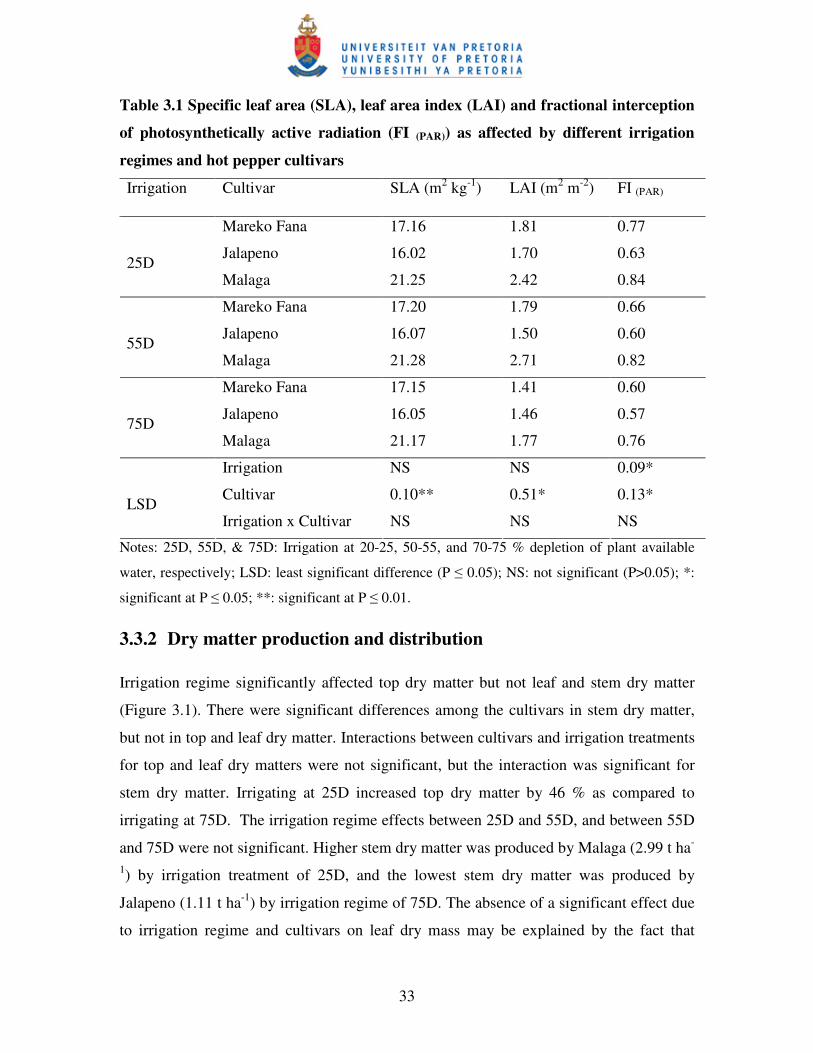
33

Table 3.1 Specific leaf area (SLA), leaf area index (LAI) and fractional interception

of photosynthetically active radiation (FI (PAR)) as affected by different irrigation

regimes and hot pepper cultivars

Irrigation

Cultivar SLA (m2 kg-1) LAI (m2 m-2) FI (PAR)

Mareko Fana 17.16 1.81 0.77

Jalapeno 16.02 1.70 0.63

25D Malaga 21.25 2.42 0.84

Mareko Fana 17.20 1.79 0.66

Jalapeno 16.07 1.50 0.60

55D Malaga 21.28 2.71 0.82

Mareko Fana 17.15 1.41 0.60

Jalapeno 16.05 1.46 0.57

75D Malaga 21.17 1.77 0.76

Irrigation NS NS 0.09*

Cultivar 0.10** 0.51* 0.13*

LSD Irrigation x Cultivar NS NS NS

Notes: 25D, 55D, & 75D: Irrigation at 20-25, 50-55, and 70-75 % depletion of plant available

water, respectively; LSD: least significant difference (P � 0.05); NS: not significant (P>0.05); *:

significant at P � 0.05; **: significant at P � 0.01.

3.3.2 Dry matter production and distribution

Irrigation regime significantly affected top dry matter but not leaf and stem dry matter

(Figure 3.1). There were significant differences among the cultivars in stem dry matter,

but not in top and leaf dry matter. Interactions between cultivars and irrigation treatments

for top and leaf dry matters were not significant, but the interaction was significant for

stem dry matter. Irrigating at 25D increased top dry matter by 46 % as compared to

irrigating at 75D. The irrigation regime effects between 25D and 55D, and between 55D

and 75D were not significant. Higher stem dry matter was produced by Malaga (2.99 t ha-

1) by irrigation treatment of 25D, and the lowest stem dry matter was produced by

Jalapeno (1.11 t ha-1) by irrigation regime of 75D. The absence of a significant effect due

to irrigation regime and cultivars on leaf dry mass may be explained by the fact that

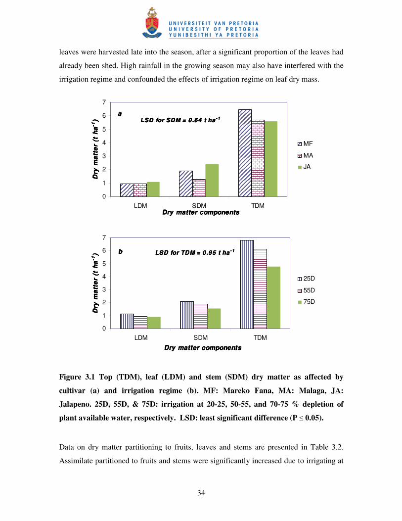
34

leaves were harvested late into the season, after a significant proportion of the leaves had

already been shed. High rainfall in the growing season may also have interfered with the

irrigation regime and confounded the effects of irrigation regime on leaf dry mass.

LSD for SDM = 0.64 t haLSD for SDM = 0.64 t haLSD for SDM = 0.64 t haLSD for SDM = 0.64 t ha - 1- 1- 1- 1

0

1

2

3

4

5

6

7

LDM SDM TDMDry matter componentsDry matter componentsDry matter componentsDry matter components

Dry

mat

ter

(t h

aD

ry m

atte

r (t

ha

Dry

mat

ter

(t h

aD

ry m

atte

r (t

ha-1-1 -1-1

)) ))

MF

MA

JA

aaaa

LSD for TDM = 0.95 t haLSD for TDM = 0.95 t haLSD for TDM = 0.95 t haLSD for TDM = 0.95 t ha - 1- 1- 1- 1

0

1

2

3

4

5

6

7

LDM SDM TDMDry matter componentsDry matter componentsDry matter componentsDry matter components

Dry

mat

ter

(t h

aD

ry m

atte

r (t

ha

Dry

mat

ter

(t h

aD

ry m

atte

r (t

ha-1-1 -1-1

)) ))

25D

55D

75D

bbbb

Figure 3.1 Top (TDM), leaf (LDM) and stem (SDM) dry matter as affected by

cultivar (a) and irrigation regime (b). MF: Mareko Fana, MA: Malaga, JA:

Jalapeno. 25D, 55D, & 75D: irrigation at 20-25, 50-55, and 70-75 % depletion of

plant available water, respectively. LSD: least significant difference (P � 0.05).

Data on dry matter partitioning to fruits, leaves and stems are presented in Table 3.2.

Assimilate partitioned to fruits and stems were significantly increased due to irrigating at

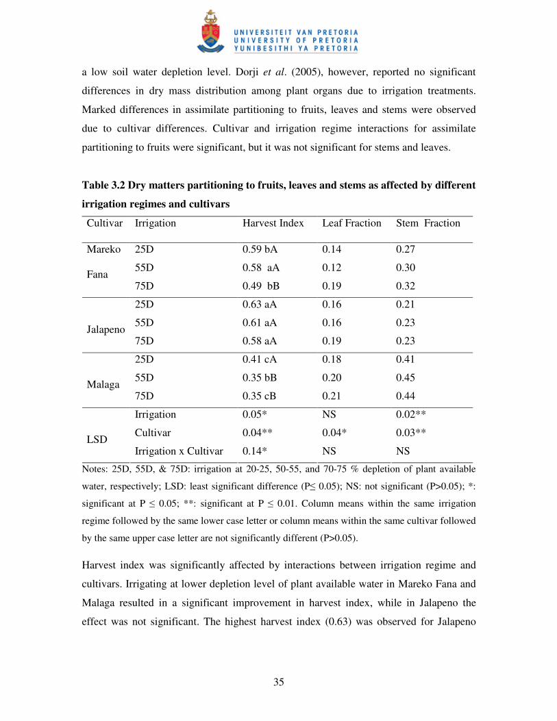
35

a low soil water depletion level. Dorji et al. (2005), however, reported no significant

differences in dry mass distribution among plant organs due to irrigation treatments.

Marked differences in assimilate partitioning to fruits, leaves and stems were observed

due to cultivar differences. Cultivar and irrigation regime interactions for assimilate

partitioning to fruits were significant, but it was not significant for stems and leaves.

Table 3.2 Dry matters partitioning to fruits, leaves and stems as affected by different

irrigation regimes and cultivars

Cultivar Irrigation Harvest Index Leaf Fraction Stem Fraction

25D 0.59 bA 0.14 0.27

55D 0.58 aA 0.12 0.30

Mareko

Fana 75D 0.49 bB 0.19 0.32

25D 0.63 aA 0.16 0.21

55D 0.61 aA 0.16 0.23

Jalapeno 75D 0.58 aA 0.19 0.23

25D 0.41 cA 0.18 0.41

55D 0.35 bB 0.20 0.45

Malaga 75D 0.35 cB 0.21 0.44

Irrigation 0.05* NS 0.02**

Cultivar 0.04** 0.04* 0.03**

LSD Irrigation x Cultivar 0.14* NS NS

Notes: 25D, 55D, & 75D: irrigation at 20-25, 50-55, and 70-75 % depletion of plant available

water, respectively; LSD: least significant difference (P� 0.05); NS: not significant (P>0.05); *:

significant at P � 0.05; **: significant at P � 0.01. Column means within the same irrigation

regime followed by the same lower case letter or column means within the same cultivar followed

by the same upper case letter are not significantly different (P>0.05).

Harvest index was significantly affected by interactions between irrigation regime and

cultivars. Irrigating at lower depletion level of plant available water in Mareko Fana and

Malaga resulted in a significant improvement in harvest index, while in Jalapeno the

effect was not significant. The highest harvest index (0.63) was observed for Jalapeno

36

under the 25D treatment, while the lowest harvest index was observed for Malaga (55D

and 75D).

Sixty percent of assimilate was portioned to fruits in Jalapeno, while it was 55 % in

Mareko Fana and 37 % by Malaga. Assimilate partitioned to leaves and stems were,

respectively, 17% and 22 % for Jalapeno, 15 % and 30% for Mareko Fana, and 20 % and

43 % for Malaga. Overall, fruits remained the major sink; accounting for more than 51 %

of the top plant dry matter mass, followed by stems (32 %) and then leaves (17%). This

result further indicated that the harvest index was significantly affected by irrigation

regime, but the effect of irrigation regime is modified by cultivar differences. The harvest

index reported here is higher than that of the 39% reported from split-root experiments with

pot grown pepper (Cantore et al., 2000), whereas it closely approaches that of the 56 %

reported from a deficit irrigation and partial root drying experiment on pepper (Dorji et al.,

2005).

The significant fruit dry yield differences among the cultivars (Table 3.3), despite the fact

that comparable top dry matters were produced by all cultivars, may be explained by the

fact that the variety with highest yields (Mareko Fana) partitioned more of its assimilates

(55%) to fruits, while the variety with lowest yield (Malaga) partitioned only 37% of its

assimilates to fruits. Moreover, the cultivar with lowest yield accumulated more than 40

% of its assimilate in stems, whose contribution to photosynthesis or fruit yield is

insignificant.

3.3.3 Yield, yield components and selected quality measures

Table 3.3 shows yield, yield components and selected quality traits as a function of

cultivar and irrigation regime. Fresh and dry fruit yields were significantly affected by

cultivar differences, and also high irrigation regime (25D) significantly increased both

fresh and dry fruit yields (Table 3.3). Cultivar and irrigation regime interactions were not

significant for both fresh and dry fruit yields, indicating that these parameters responded

to soil water level, independent of cultivar differences When dry fruit yield of the

respective cultivars are averaged over-irrigation regimes, cultivar Mareko Fana (3.60 t

ha-1) out-yielded Jalapeno (3.44 t ha-1) and Malaga (2.11 t ha-1) by 5 and 71 %,

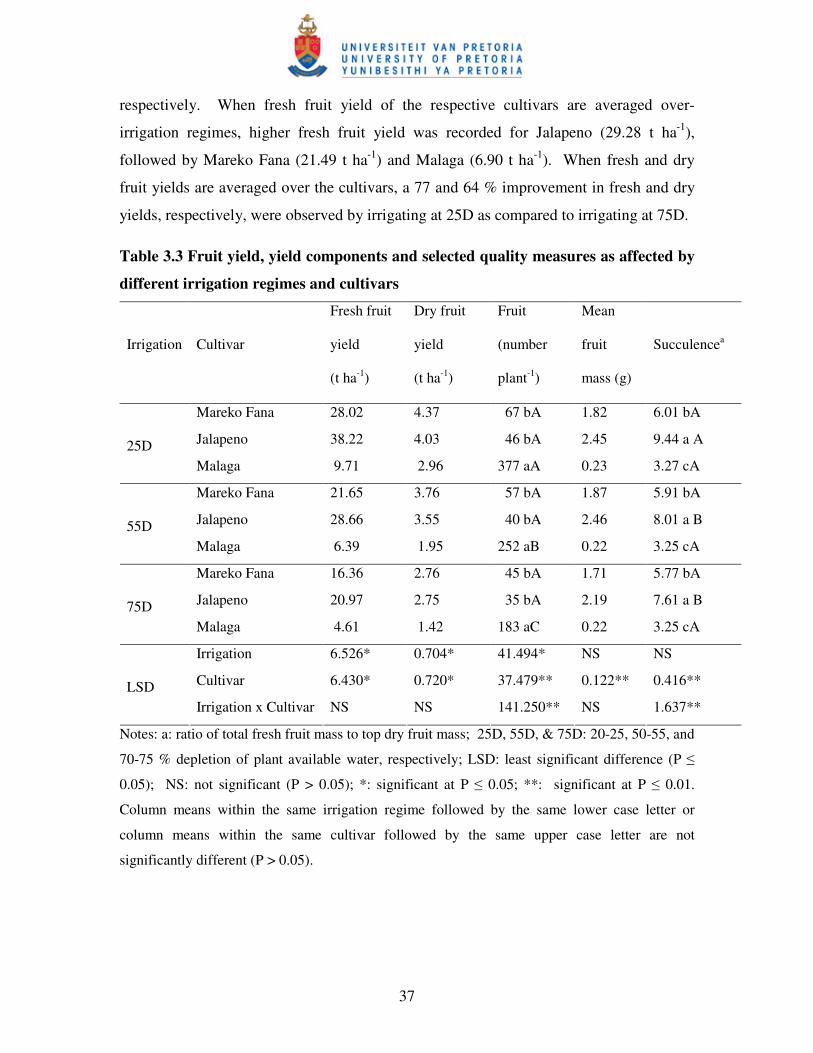
37

respectively. When fresh fruit yield of the respective cultivars are averaged over-

irrigation regimes, higher fresh fruit yield was recorded for Jalapeno (29.28 t ha-1),

followed by Mareko Fana (21.49 t ha-1) and Malaga (6.90 t ha-1). When fresh and dry

fruit yields are averaged over the cultivars, a 77 and 64 % improvement in fresh and dry

yields, respectively, were observed by irrigating at 25D as compared to irrigating at 75D.

Table 3.3 Fruit yield, yield components and selected quality measures as affected by

different irrigation regimes and cultivars

Irrigation

Cultivar

Fresh fruit

yield

(t ha-1)

Dry fruit

yield

(t ha-1)

Fruit

(number

plant-1)

Mean

fruit

mass (g)

Succulencea

Mareko Fana 28.02 4.37 67 bA 1.82 6.01 bA

Jalapeno 38.22 4.03 46 bA 2.45 9.44 a A

25D Malaga 9.71 2.96 377 aA 0.23 3.27 cA

Mareko Fana 21.65 3.76 57 bA 1.87 5.91 bA

Jalapeno 28.66 3.55 40 bA 2.46 8.01 a B

55D Malaga 6.39 1.95 252 aB 0.22 3.25 cA

Mareko Fana 16.36 2.76 45 bA 1.71 5.77 bA

Jalapeno 20.97 2.75 35 bA 2.19 7.61 a B

75D Malaga 4.61 1.42 183 aC 0.22 3.25 cA

Irrigation 6.526* 0.704* 41.494* NS NS

Cultivar 6.430* 0.720* 37.479** 0.122** 0.416**

LSD

Irrigation x Cultivar NS NS 141.250** NS 1.637**

Notes: a: ratio of total fresh fruit mass to top dry fruit mass; 25D, 55D, & 75D: 20-25, 50-55, and

70-75 % depletion of plant available water, respectively; LSD: least significant difference (P �

0.05); NS: not significant (P > 0.05); *: significant at P � 0.05; **: significant at P � 0.01.

Column means within the same irrigation regime followed by the same lower case letter or

column means within the same cultivar followed by the same upper case letter are not

significantly different (P > 0.05).

38

There were no significant differences in fresh and dry fruit yields between 25D and 55D

suggesting the possibility of employing water-saving tactics. Similarly, results elsewhere

reported the applicability of deficit irrigation in hot pepper production without compromising

yields (Kang et al., 2001; Dorji et al., 2005). However, others confirmed the sensitivity of

pepper to water stress and the beneficial effects of abundant irrigation. Costa &

Gianquinto (2002) and Beese et al. (1982) observed significant yield increases with water

rates above 100 % evapotranspiration, indicating that yield increases with more water

than the well-water control. The inconsistency of the results reported may be attributed to

differences in the cultivars (Ismail & Davies, 1997; Jaimez et al., 1999) and in the

growing conditions (Pellitero et al., 1993).

Average dry fruit mass and succulence were significantly affected by cultivar differences,

but not by irrigation regime. Cultivar and irrigation regime interactions were significant

for succulence, but not for average dry fruit mass. Fruit number per plant was

significantly affected by irrigation regime, cultivar differences and their interaction

effect. When mean dry fruit mass was averaged across irrigation regimes, Jalapeno (2.27

g) gave higher mean dry fruit mass, followed by Mareko Fana (1.80 g) and Malaga (0.22

g). However, the number of fruits produced by respective cultivars followed the reverse

order as that of mean dry fruit mass, where Malaga produced 271 fruits per plant on

average, while Mareko Fana and Jalapeno produced 56 and 41 fruits per plant,

respectively.

Although plants were irrigated at less frequent intervals under 55D and 75D than 25D,

the mean fruit mass was not affected by irrigation regime. This may be attributed to low

crop load due to high degree of flower abortion in 55D and 75D plants, compared to

those plants receiving the 25D irrigation treatment (Dorji et al., 2005). Reduction in fruit

number due to low level of soil water in 55D and 75D may have enhanced accumulation

of available assimilates in the remaining fewer fruits, maintaining the final fruit mass

comparable to 25D. Pepper plants are most sensitive to water stress during flowering and

fruit development (Katerji et al., 1993). Furthermore, the existence of a consistent inverse

relationship between mean dry fruit mass and fruit number per plant among the cultivars

39

confirms the difficulty of achieving improvement in these two parameters

simultaneously.

Jalapeno (8.4) was on average more succulent at harvest than Mareko Fana (5.9) and

Malaga (3.3). Irrigation at a low level of soil water depletion (25D) resulted in greater

succulence than when irrigating at a medium (55D) or high (75D) level of soil water

depletion. Thus Jalapeno fruits harvested from plants irrigated at 25D are recommended

for the fresh market, as these fruit exhibit highest succulence, which directly relates to hot

pepper fruit quality.

3.3.4 Soil water content, water-use and water-use efficiency

Soil water content to 0.6 m soil depth during the growing season is shown in Figure 3.2.

Soil water content within the 0.60 m soil profile decreased gradually towards the end of

the season in plots irrigated at 55D and 75D. However, soil water remained higher in the

plots irrigated at 25D. From the commencement of stress imposition (December 13) the

soil water deficit level reached below 55D on only four occasions, whereas it never

dropped below D75 due to high rainfall in the growing season. The depletion level for the

75D was higher than for 55D, and that of 55D was higher than 25D throughout the

growing season, indicating that water availability was higher for 25D than 55D, followed

by 75D.

Table 3.4 presents the components of soil water balance. The irrigation and rain in the

different irrigation treatments, i.e., 25D, 55D and 75D was 830 mm, 731 mm and 673

mm for Mareko Fana, 740 mm, 655 mm and 616 mm for Jalapeno, and 902 mm, 792 mm

and 710 mm for Malaga. The water consumption (evapotranspiration) ranged from 430

mm to 675 mm, and the observed differences in evapotranspiration among the cultivars

were as a result of the differences in the length of the growing season. The water saved

by irrigating at 75D as compared to 25D was 23 % for Mareko Fana, 20 % for Jalapeno,

and 27 % for Malaga. Similarly, by irrigating at 55D as opposed to irrigating at 25D, on

average across the cultivars, 14% of water was saved. The total irrigation events

corresponding to the different irrigation treatments, i.e., 25D, 55D and 75D were 20, 11

and 9 days in Jalapeno and 26, 13 and 9 days in Malaga and Mareko Fana.

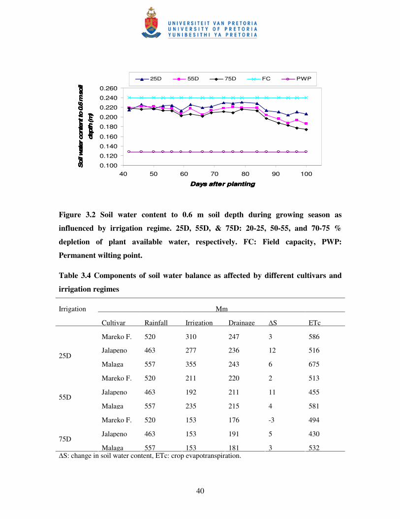
40

0.100

0.120

0.140

0.160

0.180

0.200

0.220

0.240

0.260

40 50 60 70 80 90 100

Days after plantingDays after plantingDays after plantingDays after planting

Soi

l wat

er c

onte

nt to

0.6

m s

oil

Soi

l wat

er c

onte

nt to

0.6

m s

oil

Soi

l wat

er c

onte

nt to

0.6

m s

oil

Soi

l wat

er c

onte

nt to

0.6

m s

oil

dept

h (m

)de

pth

(m)

dept

h (m

)de

pth

(m)

25D 55D 75D FC PWP

Figure 3.2 Soil water content to 0.6 m soil depth during growing season as

influenced by irrigation regime. 25D, 55D, & 75D: 20-25, 50-55, and 70-75 %

depletion of plant available water, respectively. FC: Field capacity, PWP:

Permanent wilting point.

Table 3.4 Components of soil water balance as affected by different cultivars and

irrigation regimes

Mm Irrigation

Cultivar Rainfall Irrigation Drainage �S ETc

Mareko F. 520 310 247 3 586

Jalapeno 463 277 236 12 516

25D Malaga 557 355 243 6 675

Mareko F. 520 211 220 2 513

Jalapeno 463 192 211 11 455

55D Malaga 557 235 215 4 581

Mareko F. 520 153 176 -3 494

Jalapeno 463 153 191 5 430

75D Malaga 557 153 181 3 532

�S: change in soil water content, ETc: crop evapotranspiration.

41

Table 3.5 summarizes the water-use efficiency (WUE) in terms of fresh and dry fruit

yields and top dry matter yields for all the treatments. The WUE in terms of fresh and dry

fruit yields were significantly influenced by cultivars, but WUE for top dry matter was

not affected by cultivar (Table 3.5). Irrigation regime did not affect any of the WUE

considered. The cultivar and irrigation regime interaction effects for the three WUE

considered were also not significant. Similarly, Katerji et al. (1993) using trickle

irrigation, observed no significant differences in WUE between stressed and well-

irrigated treatments. However, Kang et al. (2001) and Dorji et al. (2005) reported

significant improvement in WUE due to water stress applied. In the present study,

reduction in water application did not contribute to improvement in WUE. This is

because yield and biomass were significantly reduced due to the reduction in irrigation.

On average, the cultivar Jalapeno exhibited higher WUE in terms of fresh and dry fruit

yields, followed by Mareko Fana and Malaga. The cultivars Jalapeno and Mareko Fana

had comparable WUE in terms of top dry matter yield. The difference in WUE among the

cultivars can be explained by the fact that cultivars with high WUE reached maturity

earlier, with relatively high fresh as well as dry fruit yield. The absence of significant

differences in WUE for top dry matter production is because all three cultivars produced

comparable top dry matter yields.

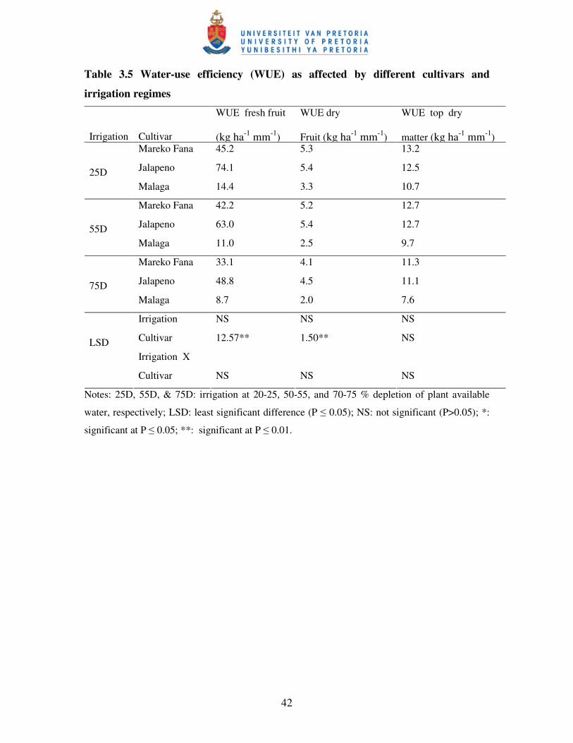
42

Table 3.5 Water-use efficiency (WUE) as affected by different cultivars and

irrigation regimes

Irrigation

Cultivar

WUE fresh fruit

(kg ha-1 mm-1)

WUE dry

Fruit (kg ha-1 mm-1)

WUE top dry

matter (kg ha-1 mm-1) Mareko Fana 45.2 5.3 13.2

Jalapeno 74.1 5.4 12.5

25D Malaga 14.4 3.3 10.7

Mareko Fana 42.2 5.2 12.7

Jalapeno 63.0 5.4 12.7

55D Malaga 11.0 2.5 9.7

Mareko Fana 33.1 4.1 11.3

Jalapeno 48.8 4.5 11.1

75D Malaga 8.7 2.0 7.6

Irrigation NS NS NS

Cultivar 12.57** 1.50** NS

Irrigation X

LSD

Cultivar NS NS NS

Notes: 25D, 55D, & 75D: irrigation at 20-25, 50-55, and 70-75 % depletion of plant available

water, respectively; LSD: least significant difference (P � 0.05); NS: not significant (P>0.05); *:


43

3.4 CONCLUSIONS

This study demonstrated that highest yield under rainfed conditions with supplemental

irrigation in Pretoria would be obtained by maintaining the depletion of soil water level

between 20 and 55%. The absence of significant differences in fresh and dry fruit yields

between 25D and 55D, suggests the potential of practicing deficit irrigation.

Despite comparable top dry biomass yields, the cultivars produced significantly different dry

and fresh fruit yields. This is due to the fact that the dry yield differences among the cultivars

were more attributed to differences in harvest index and average fruit mass, than leaf area,

top biomass or fruit number differences. The WUE did not improve by irrigating at higher

level of plant water depletion, as the corresponding yield reduction per unit water saved

outweighed the yield gain per unit water applied. Significant differences in WUE for

fresh and dry fruit yields were observed among the cultivars. This is attributed to early

maturity, high harvest index and high succulence by those cultivars with high WUE for

fresh and dry fruit yields. There were no significant interaction effects observed for most

parameters which revealed that hot pepper response to irrigation regime was the same for all

cultivars. It appears that an appropriate irrigation regime that maximizes production of hot

pepper can be devised across cultivars.

Finally, where the cost of fresh water is high, further research is recommended to establish an

irrigation regime involving deficit irrigation by quantifying the trade-off between the yield

loss that would be incurred because of irrigation at levels that are below the optimum and the

economical and ecological advantage that would be achieved by practicing deficit irrigation.

44

CHAPTER 4

RESPONSE OF HOT PEPPER (Capsicum annuum L.)

CULTIVARS TO DIFFERENT ROW SPACINGS

Abstract

A field trial was conducted in the 2004/2005 growing season at the Hatfield Experimental

Farm, University of Pretoria, to investigate the effect of different row spacings and

cultivars on growth, yield and water-use efficiency with the aim of selecting the cultivars

that are more efficient in resource utilization. Treatments were arranged in a randomized

complete block strip plot design, where the row spacings and cultivars were assigned to main

plots and sub plots, respectively. The three cultivars were Jalapeno, Malaga and Serrano, and

the two row spacings 0.45 m and 0.70 m. Treatments were replicated three times and drip

irrigation was utilized. Growth analysis, soil water content and yield measurements were

performed.

Cultivar Jalapeno (4.24 t ha-1) out-yielded Serrano (2.67 t ha-1) and Malaga (2.50 t ha-1) in

dry fruit yield. Higher fresh yield was also recorded for Jalapeno (38.61 t ha-1), followed

by Serrano (15.62 t ha-1) and Malaga (8.05 t ha-1). A 25% and 22% improvement in fresh

fruit and dry fruit yields, respectively, was observed by planting at a row spacing of 0.45

m, as compared to planting at a row spacing of 0.70 m. Fruit number per plant increased

from 112 to 127 as row spacing increased from 0.45 m to 0.70 m, indicating a

compensatory growth response by individual plants to offset yield reduction due to wide

row spacing. The high fruit dry mass recorded in Jalapeno (4.24 t ha-1), in spite of low

fruit number per plant, is attributed to its high harvest index (0.64) and high average fruit

dry mass (2.44 g). Malaga produced the highest fruit number per plant (245), but yielded

the lowest dry and fresh fruit yield due to its relatively low harvest index (0.40) and low

average fruit dry mass (0.23 g). The existence of a consistent inverse relationship

between average dry fruit mass and fruit number per plant among the cultivars confirms

the difficulty of achieving improvement in those two parameters concomitantly.

45

No significant interaction effect was observed for most parameters studied; revealing that

hot pepper response to row spacing did not depend on cultivar differences. Thus, it

appears that appropriate row spacing that maximizes production of hot pepper can be

devised across cultivars having similar growth habit to ones studied here.

Key words: Hot pepper, plant density, row spacing, water-use efficiency

46

4.1 INTRODUCTION

Hot pepper cultivars show considerable biodiversity: cultivars differ vastly in attributes

such as growth habit, length of growing season, cultural requirements, fruit size,

pigmentation and pungency (Bosland, 1992). Production and harvesting costs are high in

hot pepper, as the crop is capital- (irrigation & other inputs) and labour-intensive.

Managing production inputs and minimizing production costs are increasingly important

for profitable hot pepper production. Row spacing is one of the cultural practices that

influence productivity of a crop (Kelley & Boyhan, 2006).

Optimum plant population or in-row plant spacing studies have been conducted on bell

(Russo, 1991; Locascio & Stall, 1994), cayenne (Decoteau & Graham, 1994),

pepperoncini (Motsenbocker, 1996), paprika (Kahn et al., 1997; Cavero et al., 2001), and

pimiento peppers (Ortega et al., 2004). However, recommendations suggested by each

investigator vary widely. For instance, Decoteau & Graham (1994) reported 44 400

plants ha-1 for optimum cayenne pepper production, while Ortega et al. (2004)

recommended plant densities in the range of 100 000 to 120 000 plants ha-1 for pimiento

pepper. This is because optimum plant population density for a given species varies

depending on cultivar, input level, harvesting techniques and other cultural practices.

Generally, high density planting is associated with high yields. High density planting also

aids mechanical harvesting, as more fruits set on higher plant canopy (Decoteau &

Graham, 1994). However, disease incidence due to reduced ventilation (Karlen et al.,

1987; Stofella & Bryan, 1988) and poor colour development of fruits due to reduced light

exposure (Stofella & Bryan, 1988; Cavero et al., 2001) are some of the limitations of

high density planting. Thus, it appears that a compromise is made between yield, quality

and ease of performing cultural practices when the producer has to decide the best

planting density.

Literature reviewed so far indicated that most researchers considered only one or two

cultivars in their studies, and little information is available on how the different growth

components of pepper are affected by row spacing to ultimately determine the

performance of hot pepper cultivars. Information on how row spacing affects yield and

47

growth of different hot pepper cultivars has not been well elucidated under field

conditions in the Pretoria area. Furthermore, literature on the impact of varying the plant

population of hot pepper on canopy growth is inadequate. Cognizant of the diversity of

hot peppers and the sparse information available on plant population effects on

performance of hot pepper, a field experiment was conducted with the objective to

investigate effects of different row spacings on yield, quality and growth of hot pepper

cultivars.

48



A field experiment was conducted at the Hatfield Experimental Farm, Pretoria, South

Africa (latitude 25045’ S, longitude 28016’ E, altitude 1327 m.a.s.l.). The area has an

average annual rainfall of 670 mm, mainly from October to March (Annandale et al.,

1999). The average annual maximum air temperature for the area is 25 °C and the

average annual minimum air temperature is 12 °C. The hottest month of the year is

January, with an average maximum air temperature of 29 °C, while the coldest months

are June and July, with an average minimum air temperature of 5 °C. The soil

characteristics to 30 cm soil depth are predominately sandy clay loam with permanent

wilting point of 128 mm m-1, field capacity of 240 mm m-1 and pH of 6.5. The soil

contained 572 mg Ca, 79 mg K, 188mg Mg and 60.5 mg Na per one kg of dry soil.

Treatments were arranged in randomized complete block strip plot design, where the row

spacings and cultivars were assigned to main plot and sub plots, respectively. The two

row spacings were 0.7 x 0.4 m and 0.45 x 0.4 m, which corresponded to 35714 and 55555

plants ha-1, respectively. The three cultivars were Serrano, Jalapeno and Malaga.


Six-week-old hot pepper transplants of the respective cultivars were transplanted on 11

November, 2004. Plants were irrigated using drip irrigation for 1 hour (12.5-15.5 mm)

every other day for three weeks until plants were well established. Thereafter, the soil

profile was refilled to field capacity, every time when the measured soil water deficit

level reached 50-55% depletion of plant available water. Based on soil analysis results

and target yield, 150 kg ha-1 N, 75 kg ha-1 P and 50 kg ha-1 K were applied to all plots.

The N application was split, with 50 kg ha-1 at planting, followed by a 100 kg ha-1 top

dressing eight weeks after transplanting. Weeds were controlled manually. Fungal

diseases were controlled using Benomyl® (1H – benzimidazole) and Bravo®

(chlorothalonil) sprays, while red spider mites were controlled with Metasystox®

(oxydemeton–methyl) applied at the recommended doses.

49

4.2.3 Measurements

Eight plants from the central two rows of each plot were marked for yield measurement.

Fruits were harvested three times during the season. On the final day of harvest, all

aboveground plant parts were harvested and separated into fruits, stems and leaves and

whereafter they were oven dried at 75 °C for 72 hours to constant mass, and dry mass

was determined. Leaf area was measured with an LI 3100 belt driven leaf area meter (Li-

Cor, Lincoln, Nebraska, USA). Leaf area index was calculated from the leaf area and

ground area from which the samples were taken. Specific leaf area was calculated as the

ratio of leaf area to leaf dry mass.

The fraction of photosynthetically active radiation intercepted (FIPAR) by the canopy was

measured using a sunfleck ceptometer (Decagon Devices, Pullman, Washington, USA) a

day before harvest. The photosynthetically active radiation (PAR) measurement for a plot

consisted of three series of measurements in rapid succession. A series of measurements

consisted of one reference reading above the canopy and ten readings below the canopy.

The difference between the above canopy and below canopy PAR measurements was

used to calculate the fractional interception (FI) of PAR using the following equation

(Jovanovic & Annandale, 1999).

��

��

�−=


FI PAR 1 (4.1)




drainage and R is runoff. Drainage was estimated using SWB model, runoff was assumed

negligible as the experiment setting doses not allow free runoff.





50

4.2.4 Data analysis

Data was analyzed using the Mixed Procedure of SAS software Version 9.1 (SAS, 2003).

Treatment means were separated by the least significance difference (LSD) test at P �

0.05.

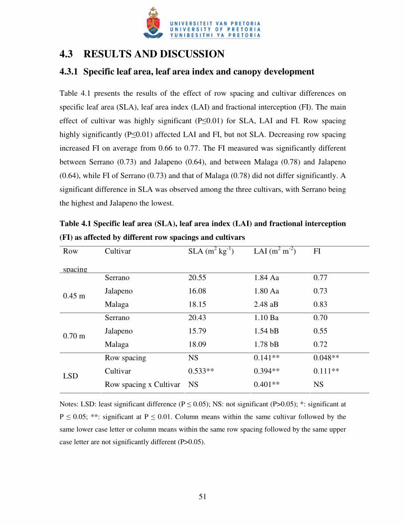
51



Table 4.1 presents the results of the effect of row spacing and cultivar differences on

specific leaf area (SLA), leaf area index (LAI) and fractional interception (FI). The main

effect of cultivar was highly significant (P�0.01) for SLA, LAI and FI. Row spacing

highly significantly (P�0.01) affected LAI and FI, but not SLA. Decreasing row spacing

increased FI on average from 0.66 to 0.77. The FI measured was significantly different

between Serrano (0.73) and Jalapeno (0.64), and between Malaga (0.78) and Jalapeno

(0.64), while FI of Serrano (0.73) and that of Malaga (0.78) did not differ significantly. A

significant difference in SLA was observed among the three cultivars, with Serrano being

the highest and Jalapeno the lowest.


(FI) as affected by different row spacings and cultivars

Row

spacing

Cultivar SLA (m2 kg-1) LAI (m2 m-2) FI

Serrano 20.55 1.84 Aa 0.77

Jalapeno 16.08 1.80 Aa 0.73

0.45 m Malaga 18.15 2.48 aB 0.83

Serrano 20.43 1.10 Ba 0.70

Jalapeno 15.79 1.54 bB 0.55

0.70 m Malaga 18.09 1.78 bB 0.72

Row spacing NS 0.141** 0.048**

Cultivar 0.533** 0.394** 0.111**

LSD Row spacing x Cultivar NS 0.401** NS

Notes: LSD: least significant difference (P � 0.05); NS: not significant (P>0.05); *: significant at

P � 0.05; **: significant at P � 0.01. Column means within the same cultivar followed by the

same lower case letter or column means within the same row spacing followed by the same upper

case letter are not significantly different (P>0.05).

52

The cultivar and row spacing interaction effect was significant for LAI, but not for SLA

and FI. Highest LAI (2.48 m2 m-2) was recorded in Malaga at a row spacing of 0.45 m,

while the lowest LAI (1.10 m2 m-2) was observed in Jalapeno at a row spacing of 0.7 m.

The relationship between LAI and FI, or SLA and LAI is not usually direct. For instance,

on average the relatively high LAI recorded for Jalapeno (1.67 m2 m-2) in relation to

Serrano (1.47 m2 m-2) did not result in higher FI for Jalapeno (0.64) as compared to

Serrano (0.73). Furthermore, the high mean SLA observed in Serrano (20.49 m2 kg-1) as

compared to Jalapeno (15.94 m2 kg-1) did not result in higher LAI for Serrano (1.47 m2 m-

2) as compared to Jalapeno (1.67 m2 m-2). This is because FI is affected not only by the

size of the canopy but also by the way in which the leaves are configured in a canopy

(Russell et al., 1990). Similarly, SLA reflects the dry leaves mass contained in a unit of

leaf area. Thus depending on cultivars’ difference, cultivars with thin leaves with similar

leaf area would have a high SLA, which is an indicator of high productivity (Wilson et

al., 1999).

The present study has shown an improved light interception as row spacing decreased

from 0.70 m to 0.45 m. Lorezo & Catilla (1995) reported also higher LAI and a marked

improvement in radiation interception as plant populations increased in hot pepper. Flénet

et al. (1996), working on four different crop species (maize, sorghum, soybean and

sunflower), reported an improvement in light interception ability as row spacing

decreased and attributed it to the even distribution of plants and hence foliage in narrower

row spacing. Taylor et al. (1982) observed no significant increase in LAI of soybean due

to higher density planting. However, light interception was consistently greater in 0.25 m

row spacing than 1.0 m row spacing, which they attributed to a more even leaf

distribution in the narrow row spacing. The robustness of SLA across different row

spacings highlights the reliability of using this crop-specific parameter in modelling of

hot pepper under varied growing conditions (Annandale et al., 1999).

4.3.2 Dry matter production and partitioning

Dry matter production as affected by row spacing and cultivar is presented in Table 4.2.

Top dry matter, leaf dry matter and stem dry matter were significantly improved as a

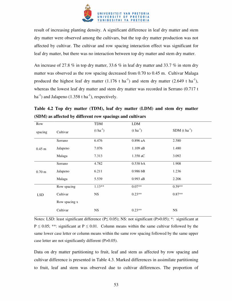
53

result of increasing planting density. A significant difference in leaf dry matter and stem

dry matter were observed among the cultivars, but the top dry matter production was not

affected by cultivar. The cultivar and row spacing interaction effect was significant for

leaf dry matter, but there was no interaction between top dry matter and stem dry matter.

An increase of 27.8 % in top dry matter, 33.6 % in leaf dry matter and 33.7 % in stem dry

matter was observed as the row spacing decreased from 0.70 to 0.45 m. Cultivar Malaga

produced the highest leaf dry matter (1.176 t ha-1) and stem dry matter (2.649 t ha-1),

whereas the lowest leaf dry matter and stem dry matter was recorded in Serrano (0.717 t

ha-1) and Jalapeno (1.358 t ha-1), respectively.

Table 4.2 Top dry matter (TDM), leaf dry matter (LDM) and stem dry matter

(SDM) as affected by different row spacings and cultivars Row

spacing

Cultivar

TDM

(t ha-1)

LDM

(t ha-1)

SDM (t ha-1)

Serrano 6.476 0.896 aA 2.580

Jalapeno 7.076 1.109 aB 1.480

0.45 m

Malaga 7.313 1.358 aC 3.092

Serrano 4.782 0.538 bA 1.908

Jalapeno 6.211 0.986 bB 1.236

0.70 m

Malaga 5.539 0.993 aB 2.206

Row spacing 1.13** 0.07** 0.59**

Cultivar NS 0.23** 0.87**

LSD

Row spacing x

Cultivar

NS

0.23**

NS

Notes: LSD: least significant difference (P� 0.05); NS: not significant (P>0.05); *: significant at

P � 0.05; **: significant at P � 0.01. Column means within the same cultivar followed by the

same lower case letter or column means within the same row spacing followed by the same upper

case letter are not significantly different (P>0.05).

Data on dry matter partitioning to fruit, leaf and stem as affected by row spacing and

cultivar difference is presented in Table 4.3. Marked differences in assimilate partitioning

to fruit, leaf and stem was observed due to cultivar differences. The proportion of

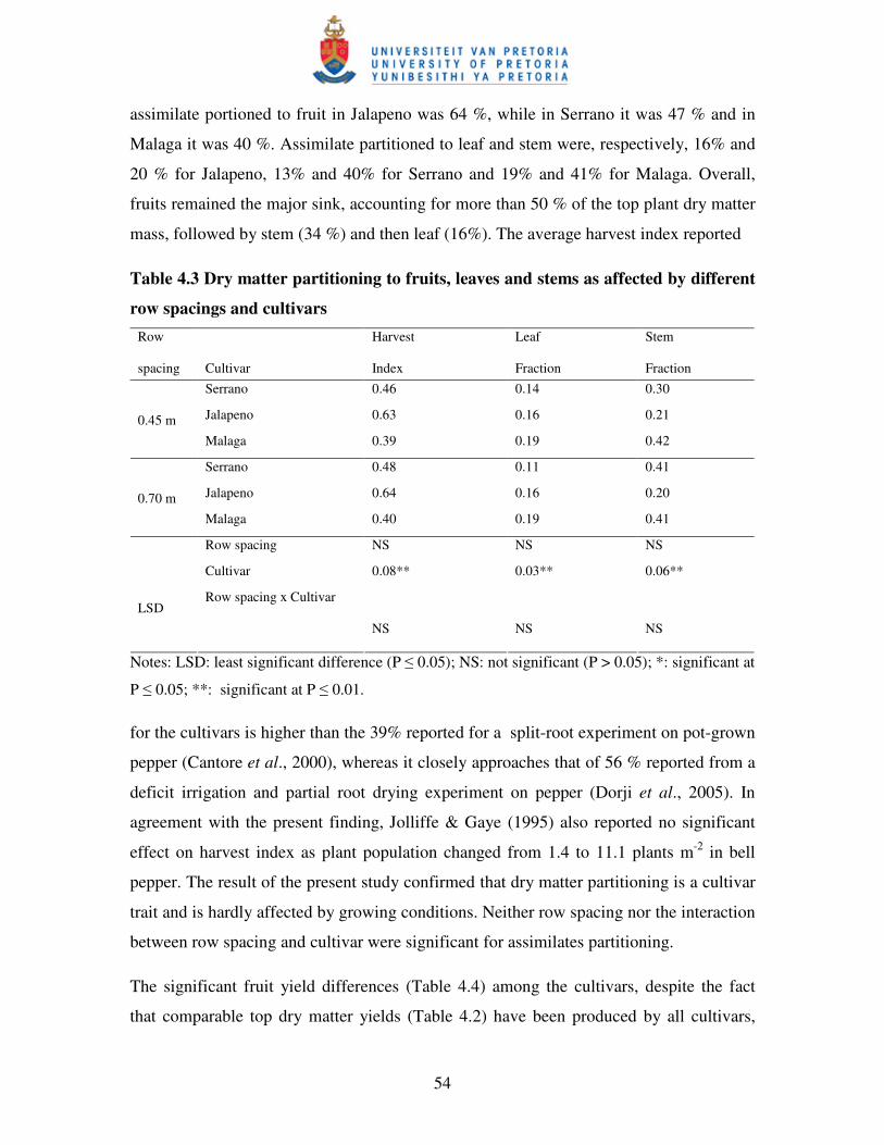
54

assimilate portioned to fruit in Jalapeno was 64 %, while in Serrano it was 47 % and in

Malaga it was 40 %. Assimilate partitioned to leaf and stem were, respectively, 16% and

20 % for Jalapeno, 13% and 40% for Serrano and 19% and 41% for Malaga. Overall,

fruits remained the major sink, accounting for more than 50 % of the top plant dry matter

mass, followed by stem (34 %) and then leaf (16%). The average harvest index reported

Table 4.3 Dry matter partitioning to fruits, leaves and stems as affected by different

row spacings and cultivars Row

spacing

Cultivar

Harvest

Index

Leaf

Fraction

Stem

Fraction Serrano 0.46 0.14 0.30

Jalapeno 0.63 0.16 0.21

0.45 m Malaga 0.39 0.19 0.42

Serrano 0.48 0.11 0.41

Jalapeno 0.64 0.16 0.20

0.70 m Malaga 0.40 0.19 0.41

Row spacing NS NS NS

Cultivar 0.08** 0.03** 0.06**

LSD Row spacing x Cultivar

NS

NS

NS

Notes: LSD: least significant difference (P � 0.05); NS: not significant (P > 0.05); *: significant at

P � 0.05; **: significant at P � 0.01.

for the cultivars is higher than the 39% reported for a split-root experiment on pot-grown

pepper (Cantore et al., 2000), whereas it closely approaches that of 56 % reported from a

deficit irrigation and partial root drying experiment on pepper (Dorji et al., 2005). In

agreement with the present finding, Jolliffe & Gaye (1995) also reported no significant

effect on harvest index as plant population changed from 1.4 to 11.1 plants m-2 in bell

pepper. The result of the present study confirmed that dry matter partitioning is a cultivar

trait and is hardly affected by growing conditions. Neither row spacing nor the interaction

between row spacing and cultivar were significant for assimilates partitioning.

The significant fruit yield differences (Table 4.4) among the cultivars, despite the fact

that comparable top dry matter yields (Table 4.2) have been produced by all cultivars,

55

may be explained by the fact that top yielding cultivar (Jalapeno) partitioned more of its

assimilates (64%) to fruit, while cultivar with lowest fruit yield (Malaga) accumulated

only 40% of its assimilates in fruits (Table 4.3). Moreover, cultivar Malaga, with lowest

yield, accumulated more than 41% of assimilates in stems, which contributed

insignificantly to photosynthesis or fruit yield.

4.3.3 Fruit yield, yield components and selected quality measures

Table 4.4 shows yield, yield components and selected quality measures as a function of

row spacing and cultivar difference. Fresh and dry fruit yields were significantly affected

by cultivar differences. High planting density significantly increased both fresh and dry

fruit yields (Table 4.4). Cultivar and row spacing interaction was not significant for both

fresh and dry fruit yields, indicating that these parameters responded to row spacing

treatment independent of cultivar differences.

Cultivar Jalapeno (4.24 t ha-1) out-yielded Serrano (2.67 t ha-1) and Malaga (2.50 t ha-1)

by 59 % and 69 %, respectively, in dry fruit yield. Higher fresh fruit yield was recorded

for Jalapeno (38.61 t ha-1), followed by Serrano (15.62 t ha-1) and Malaga (8.05 t ha-1). A

25% improvement in fresh fruit and 22% dry fruit yields were observed by planting at

row a spacing of 0.45 m, as compared to row spacing of 0.70 m.

Fruit number per plant was significantly affected by row spacing and cultivar. Average

dry fruit mass and succulence were significantly affected by cultivar differences, but not

by row spacing. Cultivar and row spacing interaction effect was not significant for fruit

number per plant, average fruit mass and succulence.

Fruit number per plant increased from 112 to 127 as row spacing increased from 0.45 m

to 0.70 m, indicating a compensatory growth response by individual plants to offset the

yield reduction due to wider row spacing. The higher productivity observed due to

narrow row spacing as compared to wide row spacing is attributed to higher top dry mass

and fruit dry mass per unit area of land. The cumulative compensatory growths effects

(fruit number per plant, average fruit mass, individual plant dry matter production)

observed for wide row spacing were not adequate enough to offset the yield reduction

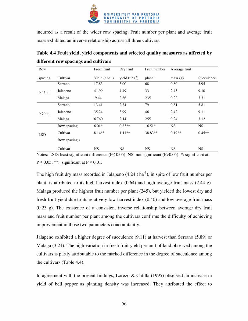
56

incurred as a result of the wider row spacing. Fruit number per plant and average fruit

mass exhibited an inverse relationship across all three cultivars.

Table 4.4 Fruit yield, yield components and selected quality measures as affected by

different row spacings and cultivars Row

spacing

Cultivar

Fresh fruit

Yield (t ha-1)

Dry fruit

yield (t ha-1)

Fruit number

plant-1

Average fruit

mass (g)

Succulence Serrano 17.83 3.00 68 0.80 5.95

Jalapeno 41.99 4.49 33 2.45 9.10

0.45 m Malaga 9.44 2.86 235 0.22 3.31

Serrano 13.41 2.34 79 0.81 5.81

Jalapeno 35.24 3.99 46 2.42 9.11

0.70 m Malaga 6.760 2.14 255 0.24 3.12

Row spacing 6.01* 0.83** 16.51* NS NS

Cultivar 8.14** 1.11** 38.83** 0.19** 0.45**

LSD

Row spacing x

Cultivar

NS

NS

NS

NS

NS



The high fruit dry mass recorded in Jalapeno (4.24 t ha-1), in spite of low fruit number per

plant, is attributed to its high harvest index (0.64) and high average fruit mass (2.44 g).

Malaga produced the highest fruit number per plant (245), but yielded the lowest dry and

fresh fruit yield due to its relatively low harvest index (0.40) and low average fruit mass

(0.23 g). The existence of a consistent inverse relationship between average dry fruit

mass and fruit number per plant among the cultivars confirms the difficulty of achieving

improvement in those two parameters concomitantly.

Jalapeno exhibited a higher degree of succulence (9.11) at harvest than Serrano (5.89) or

Malaga (3.21). The high variation in fresh fruit yield per unit of land observed among the

cultivars is partly attributable to the marked difference in the degree of succulence among

the cultivars (Table 4.4).

In agreement with the present findings, Lorezo & Catilla (1995) observed an increase in

yield of bell pepper as planting density was increased. They attributed the effect to

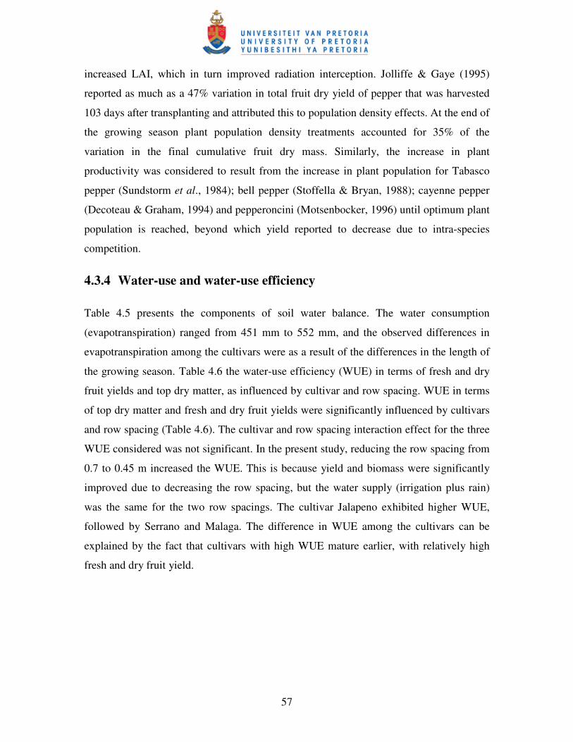
57

increased LAI, which in turn improved radiation interception. Jolliffe & Gaye (1995)

reported as much as a 47% variation in total fruit dry yield of pepper that was harvested

103 days after transplanting and attributed this to population density effects. At the end of

the growing season plant population density treatments accounted for 35% of the

variation in the final cumulative fruit dry mass. Similarly, the increase in plant

productivity was considered to result from the increase in plant population for Tabasco

pepper (Sundstorm et al., 1984); bell pepper (Stoffella & Bryan, 1988); cayenne pepper

(Decoteau & Graham, 1994) and pepperoncini (Motsenbocker, 1996) until optimum plant

population is reached, beyond which yield reported to decrease due to intra-species

competition.

4.3.4 Water-use and water-use efficiency

Table 4.5 presents the components of soil water balance. The water consumption

(evapotranspiration) ranged from 451 mm to 552 mm, and the observed differences in

evapotranspiration among the cultivars were as a result of the differences in the length of

the growing season. Table 4.6 the water-use efficiency (WUE) in terms of fresh and dry

fruit yields and top dry matter, as influenced by cultivar and row spacing. WUE in terms

of top dry matter and fresh and dry fruit yields were significantly influenced by cultivars

and row spacing (Table 4.6). The cultivar and row spacing interaction effect for the three

WUE considered was not significant. In the present study, reducing the row spacing from

0.7 to 0.45 m increased the WUE. This is because yield and biomass were significantly

improved due to decreasing the row spacing, but the water supply (irrigation plus rain)

was the same for the two row spacings. The cultivar Jalapeno exhibited higher WUE,

followed by Serrano and Malaga. The difference in WUE among the cultivars can be

explained by the fact that cultivars with high WUE mature earlier, with relatively high

fresh and dry fruit yield.

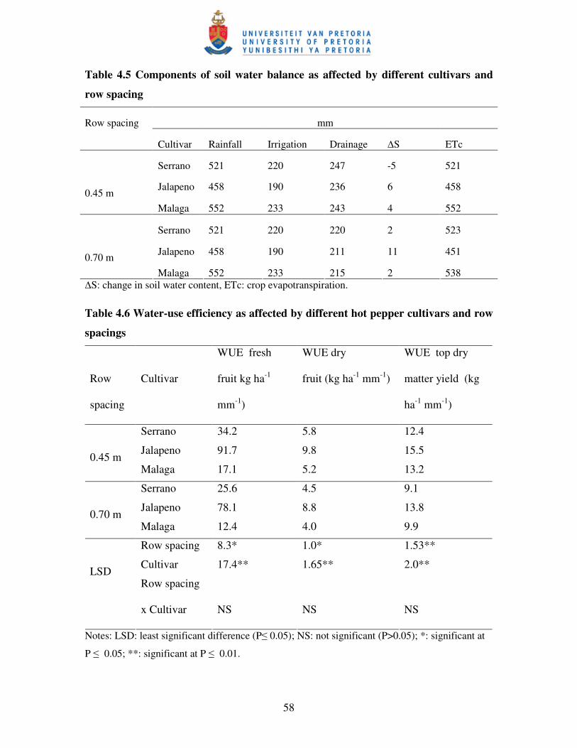
58

Table 4.5 Components of soil water balance as affected by different cultivars and

row spacing

mm Row spacing

Cultivar Rainfall Irrigation Drainage �S ETc

Serrano 521 220 247 -5 521

Jalapeno 458 190 236 6 458

0.45 m Malaga 552 233 243 4 552

Serrano 521 220 220 2 523

Jalapeno 458 190 211 11 451

0.70 m Malaga 552 233 215 2 538

�S: change in soil water content, ETc: crop evapotranspiration.

Table 4.6 Water-use efficiency as affected by different hot pepper cultivars and row

spacings

Row

spacing

Cultivar

WUE fresh

fruit kg ha-1

mm-1)

WUE dry

fruit (kg ha-1 mm-1)

WUE top dry

matter yield (kg

ha-1 mm-1)

Serrano 34.2 5.8 12.4

Jalapeno 91.7 9.8 15.5

0.45 m Malaga 17.1 5.2 13.2

Serrano 25.6 4.5 9.1

Jalapeno 78.1 8.8 13.8

0.70 m Malaga 12.4 4.0 9.9

Row spacing 8.3* 1.0* 1.53**

Cultivar 17.4** 1.65** 2.0**

LSD

Row spacing

x Cultivar

NS

NS

NS



59

4.4. CONCLUSIONS

Results from the present study indicate that high density planting markedly increased

growth and yield per unit area. Except fruit number per plant, yield components such as

average fruit mass and harvest index were unaffected by row spacing. This indicates that

the change in those important yield compensation processes were not adequate to offset

the yield reduction due to wide row spacing planting. Thus, the yield increment recorded

in the narrow row spacing is due to high biomass production per unit area, which in turn

is attributable to the improved light interception in those plants planted in narrow row

spacing.

Although all cultivars produced comparable top dry biomass, dry and fresh fruit yields

were significantly different among the cultivars. Malaga, a cultivar with the highest leaf

area, leaf mass and fruit number per plant, yielded the least. Jalapeno, a cultivar with the

highest harvest index and average fruit mass, produced the highest fresh and dry fruit

yields. Thus, the yield difference among the cultivars was more attributable to differences

in harvest index and average fruit mass rather than leaf area, top biomass or fruit number

differences. Hot pepper breeders working on yield improvement should target harvest

index and average fruit mass in their effort to breed high yielding cultivars. The wide gap

in fresh fruit yield per unit land among the cultivars is attributed to the marked difference

among the cultivar in their succulence at harvest. High density planting by virtue of its

high yield per unit area resulted in improved water-use efficiency. Cultivars with high

water-use efficiency can be obtained by selecting those that mature earlier with relatively

high fresh and dry fruit yield.

No significant interaction effects were observed for most parameters studied; revealing

that hot pepper response to row spacing did not depend on cultivar differences. Thus, it

appears that appropriate row spacing, which maximizes production of hot pepper, can be

devised across cultivars having similar growth habit with the ones considered in this

study.

60

CHAPTER 5

EFFECTS OF ROW SPACINGS AND IRRIGATION

REGIMES ON GROWTH AND YIELD OF HOT PEPPER

(Capsicum annuum L. CV ‘CAYENNE LONG SLIM’)

Abstract

A rainshelter trial was conducted in the 2004/2005 growing season at the Hatfield

experimental farm, Pretoria, to investigate the effect of row spacings and irrigation

regimes on yield, dry matter production and partitioning, and water-use efficiency of hot

pepper. A factorial combination of two row spacings (0.45 m and 0.7 m) and three

irrigation regimes, based on the measure of depletion of plant available water (PAW)

(25D: 20-25% depletion of PAW; 55D: 50-55% depletion of PAW; and 75D: 70-75%

depletion of PAW) constituted the treatments. The trial was arranged in a randomized

complete block design with three replications. Drip irrigation was utilized. Growth

analysis, soil water content and yield measurements were made.

Fresh fruit yield increased by 66 % and dry fruit yield increased by 51 % when planting

at 0.45 m row spacing compared to 0.7 m row spacing. Similarly, fresh fruit yield

increased by 49 % and dry fruit yield increased by 46 % by irrigating at 25D, as

compared to 75D. Fruit number per plant significantly increased from 70 to 100 as

irrigation regimes changed from 75D to 25D. Planting at 0.45 m row spacing

significantly improved water-use efficiency (WUE) for both fresh and dry fruit yields.

Higher WUE (16.4 kg ha-1 mm-1) in terms of top dry matter was observed for the 0.45 m

row spacing irrigated at 75D, while the least WUE (8.5 kg ha-1 mm-1) was found for 0.7

m row spacing irrigated at 55D. Irrigating at 25D as compared to 75D significantly

increased the assimilate partitioned to fruit, while the assimilate partitioned to leaf was

significantly decreased. Row spacing did not markedly affect assimilate partitioning, and

there was also no interaction effect of row spacing and irrigation regime. The extent of

LAI reduction due to water stress was expressed more in the 0.7 m row spacing than

61

with the 0.45 m row spacing. Average fruit mass, succulence and specific leaf area were

not affected by row spacing or irrigation regime.

It was concluded that yield loss could be prevented by irrigating at 25D, confirming the

sensitivity of the crop to even mild water stress. Furthermore, the absence of interaction

effects for most parameters suggested that appropriate irrigation regime to maximize hot

pepper productivity can be devised across row spacing.

Key words: Hot pepper, irrigation regime, row spacing, water-use efficiency

62

5.1 INTRODUCTION

Many countries of the arid and semi-arid regions of the world are becoming more prone

to water deficit in crop production and their future agricultural industry is at stake, unless

judicious use of water in agriculture is implemented. Deficit irrigation, the deliberate and

systematic under-irrigation of crops, is one of the possible water-saving strategies

(English & Raja, 1996). It usually increases the water-use efficiency of a crop by

reducing evapotranspiration, but produces yields that are comparable to that of a fully

irrigated crop. Deficit irrigation could also help to minimize leaching of nutrients and

pesticides into groundwater (Home et al., 2002). South Africa has endorsed the concept

of deficit irrigation in such a way that irrigation planning be based on a ‘50%

dependable’ supply of water (Chitale, 1987). However, before implementing such

recommendations for all crops there is a need to justify the losses and benefits from

deficit irrigation, especially for water deficit sensitive crops like Capsicum species.

Hot pepper (Capsicum annuum L.) is a high value cash crop of which cultivation is

confined to warm and semi-arid regions of the world. A shallow root system (Dimitrov

& Ovtcharrova, 1995), high stomatal density, a large transpiring leaf surface and the

elevated stomata opening, predisposes the pepper plant to water stress (Wein, 1998;

Delfine et al., 2000). Therefore, before employing deficit irrigation as a water-saving

strategy, an intensive study should be made to ascertain the practicality of such a

strategy.

Deficit irrigation has been studied on hot pepper with varied responses. Research

findings documented by various researchers indicated a marked variability in pepper

response to water stress, although overall, irrigation increased yield substantially (Batal

& Smittle, 1981; Beese et al., 1982; Pellitero et al., 1993; Costa & Gianquinto, 2002).

Deficit irrigation has been investigated mainly for Capsicum species without considering

other factors that would affect growth and development of plants. However, water

requirements of plants vary for different cultivars (Ismail & Davies, 1997; Jaimez et al.,

1999; Collino et al., 2000), nitrogen fertilization (Ogola et al., 2002; Rockström, 2003),

63

and irrigation methods (Xie et al., 1999; Antony & Singandhupe, 2004). Likewise, plant

population density was reported to impact the water consumption behaviour of plants

(Taylor, 1980; Tan et al., 1983; Ritchie & Basso, 2008). Under low water supply, high

plant population did not affect yield per unit area, whereas when water availability was

not limited, high plant population is produced optimum yield (Taylor et al., 1982; Tan et

al., 1983; Ritchie & Basso, 2008).

Information on frequency and quantity of irrigation water and the effects of deficit

irrigation on yield and growth of the hot pepper plant has not been well investigated

under field conditions in Pretoria. Furthermore, literature on the impact of varying the

plant population of hot pepper and its interaction with different irrigation regimes is

lacking. Irrigating at appropriate depletion of plant available soil water coupled with the

optimum row spacing contributes to water-saving without scarifying yield. Thus, it was

hypothesized that the correct combination of row spacing and irrigation regime would

improve hot pepper yield and water-use efficiency. Therefore, this experiment was

conducted with the objective to investigate the effect of plant density and irrigation

regime on yield, dry mass production and water-use efficiency.

64



An experiment was conducted under a rain shelter at the Hatfield Experimental Farm,

University of Pretoria, South Africa (latitude 25045’ S, longitude 28016’ E, altitude 1327

m.a.s.l.). The area has an average annual rainfall of 670 mm, mainly from October to

March (Annandale et al., 1999). The average annual maximum air temperature for the

area is 25 °C and the average annual minimum air temperature is 12 °C. The hottest

month of the year is January, with an average maximum air temperature of 29 °C, while

the coldest months are June and July, with an average minimum air temperature of 5 °C.

The top 30 cm soil layer has a sandy clay loam texture, with permanent wilting point of

151 mm m-1, a field capacity of 270 mm m-1 and pH (H2O) of 6.4. The soil contained

2340 mg kg-1 Ca, 155 mg kg-1 K, 967 mg kg-1 Mg and 196 mg kg-1 Na.

Treatment consisted of a factorial combination of two row spacings and three irrigation

regimes. The two inter-row spacings were 0.7 m and 0.45 m, with intra-row spacing of

0.4 m, which corresponded to population of 35714 and 55555 plants ha-1. The three

irrigation regimes were: High irrigation regime (25D, irrigated when 20-25 % depletion

of plant available water (DPAW) was reached), medium irrigation regime (55D, irrigated

when 50-55 % DPAW was reached) and low irrigation regime (75D, irrigated when 70-

75 % DPAW was reached). The plant available water was measured to 0.6 m soil profile.

Treatments were arranged in a randomized complete block design with three replicates.

Plots consisted of five rows of 2.4 m in length.


Seven-week-old hot pepper transplants of cultivar ‘Cayenne Long Slim’ were

transplanted on 19 November 2004. The plants were irrigated for one hour (12.5-15.5

mm) every other day for three weeks until plants were well established. Thereafter,

plants were irrigated to field capacity each time the predetermined soil water deficit was

reached. Weeds were controlled manually. Benomyl® (1H – benzimidazole) and

Bravo® (chlorothalonil) were applied as preventive sprays for fungal diseases, while red

65

spider mites were controlled using Metasystox® (oxydemeton–methyl) applied at the

recommended doses. The N application was split, with 50 kg ha-1 at planting, followed by

a 100 kg ha-1 top dressing eight weeks after transplanting. No P was applied, as the soil

analysis showed sufficient P in the soil, while 50 kg ha-1 K was applied at planting. The

rain shelter was left open day and night until 24 days after transplanting (until the plants

were well established) where-after it was closed at nighttime and daytime only during

periods of rainfall.

5.2.3 Measurements

Soil water deficit measurements were made using a neutron water meter model 503DR

CPN Hydroprobe (Campbell Pacific Nuclear, California, USA). The neutron water meter

was calibrated for the site. Readings were taken twice a week from access tubes

installed at the middle of each plot and positioned between rows, for 0 .2 m soil layers to

1.0 m depth.

Eight plants from the central two rows were marked for yield measurement. Fruits were

harvested three times during the season. On the final day of harvest all aboveground

plant parts were removed and separated into fruits, stems and leaves, and then oven dried

at 75 °C for 72 hours to constant mass. Leaf area index was calculated from the leaf area

and ground area from which the samples were taken. Leaf area was measured with an LI

3100 belt driven leaf meter (Li-Cor, Lincoln, Nebraska, USA) on fresh leaf samples.

Specific leaf area was calculated as the ratio of leaf area to leaf dry mass. Water-use

efficiency was calculated for top dry matter, fresh fruit mass and fruit dry mass yields by

calculating the ratio between the respective parameter yields and total water-use (rainfall

and irrigation during the season).

The fraction of photosynthetically active radiation (FIPAR) intercepted by the canopy was

measured using a sunfleck ceptometer (Decagon Devices, Pullman, Washington, USA).

The PAR measurement for a plot consisted of three series of measurements in rapid

succession. A series of measurements consisted of one reference reading above the

canopy and ten readings below the canopy. The difference between the above canopy

66

and below canopy PAR measurements was used to calculate the fractional interception

(FI) of PAR using the following equation:

��

��

�−=


FI PAR 1 (5.1)




drainage and R is runoff. Drainage and runoff were assumed negligible as the irrigation

amount was to refill deficit to field capacity.





5.2.4 Data analysis

The data were analyzed using the GLM procedure of SAS software Version 9.1 (SAS,

2003). Treatment means were separated by the least significance difference (LSD) test at P

� 0.05.

67



Table 5.1 presents results on the effect of row spacings and irrigation regimes on

fractional interception of photosynthetically active radiation (FIPAR), leaf area index

(LAI) and specific leaf area (SLA). Both row spacing and irrigation regime significantly

affected FI and LAI, but not SLA. The interaction effect was significant for FI, but not

for LAI and SLA. The lack of variability of SLA across different row spacings and

irrigation regimes highlights the reliability of using this crop-specific parameter in

modelling of hot pepper under varied growing conditions (Annandale et al., 1999).

Decreasing row spacing (increasing planting density) increased mean FI from 0.69 to

0.79, while it increased mean LAI from 1.48 to 2.29 m2 m-2. Similarly, irrigating at 25D

relative to irrigating at 75D, increased mean FI from 0.63 to 0.83, while mean LAI

increased from 1.37 to 2.11m2 m-2. The highest FI (0.86) and LAI (2.63 m2 m-2) values

were achieved for plants irrigated at 25D and planted at 0.45 m row spacing. On the other

hand, the lowest FI (0.60) and LAI (1.39 m2 m-2) values were observed for plants

irrigated at 75D and planted at 0.7 m row spacing.

High irrigation regime increased FI and LAI by improving the canopy size of individual

plants as evidenced from high leaf dry mass produced due to frequent irrigation (Figure

5.1). In agreement with the present results, Tesfaye et al. (2006), working on chickpea,

cowpea and common bean, also observed a reduction in both FI and LAI due to water

stress. Joel et al. (1997) indicated that FI could be reduced as much as 70 % due to water

stress in sunflower. They attributed the reduction in FI to the corresponding reduction in

LAI caused by water stress. LAI decline caused by water stress was also reported for

potato (Kashyap & Panda, 2003).

Lorenzo & Castilla, (1995) also reported high LAI and marked improvement in radiation

interception as plant population increased in hot pepper. Working on four different

species (maize, sorghum, soybean and sunflower), Flénet et al. (1996) reported

improvement in light interception ability of these crops in narrow rows and attributed it to

a more even distribution of plants and hence foliage. Taylor et al. (1982) observed a

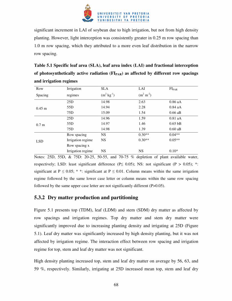
68

significant increment in LAI of soybean due to high irrigation, but not from high density

planting. However, light interception was consistently greater in 0.25 m row spacing than

1.0 m row spacing, which they attributed to a more even leaf distribution in the narrow

row spacing.


of photosynthetically active radiation (FIPAR) as affected by different row spacings

and irrigation regimes Row

Spacing

Irrigation

regimes

SLA

(m2 kg-1)

LAI

(m2 m-2)

FIPAR

25D 14.98 2.63 0.86 aA 55D 14.94 2.28 0.84 aA

0.45 m 75D 15.09 1.54 0.66 aB 25D 14.96 1.59 0.81 aA 55D 14.97 1.46 0.65 bB

0.7 m 75D 14.98 1.39 0.60 aB Row spacing NS 0.30** 0.04** Irrigation regime NS 0.30** 0.05** Row spacing x

LSD

Irrigation regime NS NS 0.10*

Notes: 25D, 55D, & 75D: 20-25, 50-55, and 70-75 % depletion of plant available water,

respectively; LSD: least significant difference (P� 0.05); NS: not significant (P > 0.05); *:

significant at P � 0.05; * *: significant at P � 0.01. Column means within the same irrigation

regime followed by the same lower case letter or column means within the same row spacing

followed by the same upper case letter are not significantly different (P>0.05).

5.3.2 Dry matter production and partitioning

Figure 5.1 presents top (TDM), leaf (LDM) and stem (SDM) dry matter as affected by

row spacings and irrigation regimes. Top dry matter and stem dry matter were

significantly improved due to increasing planting density and irrigating at 25D (Figure

5.1). Leaf dry matter was significantly increased by high density planting, but it was not

affected by irrigation regime. The interaction effect between row spacing and irrigation

regime for top, stem and leaf dry matter was not significant.

High density planting increased top, stem and leaf dry matter on average by 56, 63, and

59 %, respectively. Similarly, irrigating at 25D increased mean top, stem and leaf dry

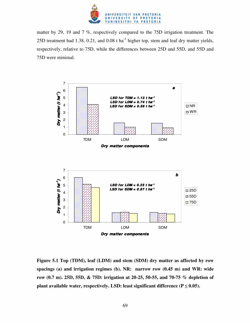
69

matter by 29, 19 and 7 %, respectively compared to the 75D irrigation treatment. The

25D treatment had 1.38, 0.21, and 0.08 t ha-1 higher top, stem and leaf dry matter yields,

respectively, relative to 75D, while the differences between 25D and 55D, and 55D and

75D were minimal.

LSD for TDM = 1.13 t haLSD for TDM = 1.13 t haLSD for TDM = 1.13 t haLSD for TDM = 1.13 t ha -1-1-1-1

LSD for LDM = 0.74 t haLSD for LDM = 0.74 t haLSD for LDM = 0.74 t haLSD for LDM = 0.74 t ha -1-1-1-1

LSD for SDM = 0.59 t haLSD for SDM = 0.59 t haLSD for SDM = 0.59 t haLSD for SDM = 0.59 t ha -1 -1 -1 -1

0

1

2

3

4

5

6

7

TDM LDM SDM

Dry matter componentsDry matter componentsDry matter componentsDry matter components

Dry

mat

ter

(t h

aD

ry m

atte

r (t

ha

Dry

mat

ter

(t h

aD

ry m

atte

r (t

ha-1-1 -1-1

)) ))

NR

WR

aaaa

LSD for LDM = 0.23 t haLSD for LDM = 0.23 t haLSD for LDM = 0.23 t haLSD for LDM = 0.23 t ha -1-1-1-1

LSD for SDM = 0.87 t haLSD for SDM = 0.87 t haLSD for SDM = 0.87 t haLSD for SDM = 0.87 t ha -1 -1 -1 -1

0

1

2

3

4

5

6

7

TDM LDM SDM

Dry matter componentsDry matter componentsDry matter componentsDry matter components

Dry

mat

ter

(t h

aD

ry m

atte

r (t

ha

Dry

mat

ter

(t h

aD

ry m

atte

r (t

ha-1-1 -1-1

)) ))

25D

55D

75D

bbbb

Figure 5.1 Top (TDM), leaf (LDM) and stem (SDM) dry matter as affected by row

spacings (a) and irrigation regimes (b). NR: narrow row (0.45 m) and WR: wide

row (0.7 m). 25D, 55D, & 75D: irrigation at 20-25, 50-55, and 70-75 % depletion of

plant available water, respectively. LSD: least significant difference (P � 0.05).

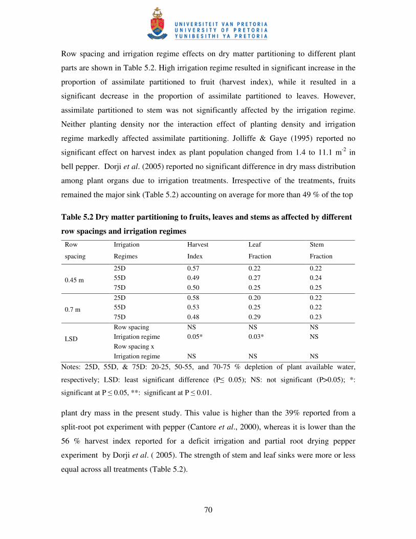
70

Row spacing and irrigation regime effects on dry matter partitioning to different plant

parts are shown in Table 5.2. High irrigation regime resulted in significant increase in the

proportion of assimilate partitioned to fruit (harvest index), while it resulted in a

significant decrease in the proportion of assimilate partitioned to leaves. However,

assimilate partitioned to stem was not significantly affected by the irrigation regime.

Neither planting density nor the interaction effect of planting density and irrigation

regime markedly affected assimilate partitioning. Jolliffe & Gaye (1995) reported no

significant effect on harvest index as plant population changed from 1.4 to 11.1 m-2 in

bell pepper. Dorji et al. (2005) reported no significant difference in dry mass distribution

among plant organs due to irrigation treatments. Irrespective of the treatments, fruits

remained the major sink (Table 5.2) accounting on average for more than 49 % of the top

Table 5.2 Dry matter partitioning to fruits, leaves and stems as affected by different

row spacings and irrigation regimes Row

spacing

Irrigation

Regimes

Harvest

Index

Leaf

Fraction

Stem

Fraction

25D 0.57 0.22 0.22 55D 0.49 0.27 0.24

0.45 m 75D 0.50 0.25 0.25 25D 0.58 0.20 0.22 55D 0.53 0.25 0.22

0.7 m 75D 0.48 0.29 0.23 Row spacing NS NS NS Irrigation regime 0.05* 0.03* NS

LSD Row spacing x

Irrigation regime NS NS NS


respectively; LSD: least significant difference (P� 0.05); NS: not significant (P>0.05); *:

significant at P � 0.05, **: significant at P � 0.01.

plant dry mass in the present study. This value is higher than the 39% reported from a

split-root pot experiment with pepper (Cantore et al., 2000), whereas it is lower than the

56 % harvest index reported for a deficit irrigation and partial root drying pepper

experiment by Dorji et al. ( 2005). The strength of stem and leaf sinks were more or less

equal across all treatments (Table 5.2).

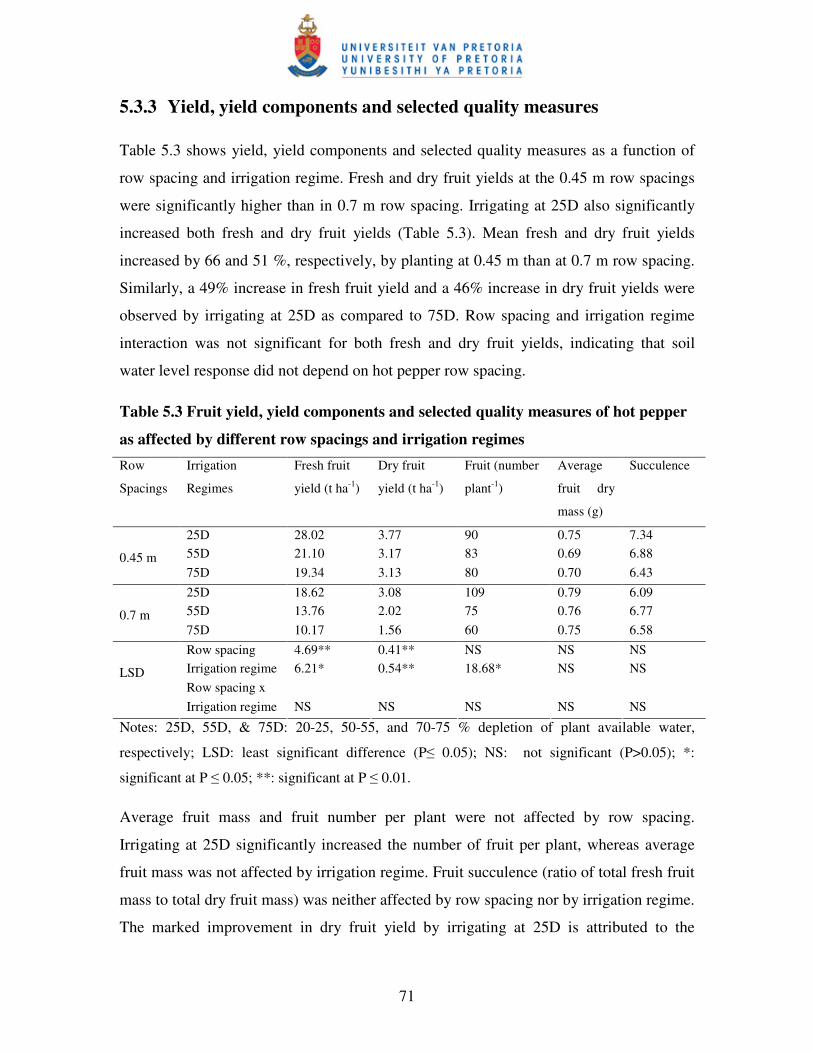
71

5.3.3 Yield, yield components and selected quality measures

Table 5.3 shows yield, yield components and selected quality measures as a function of

row spacing and irrigation regime. Fresh and dry fruit yields at the 0.45 m row spacings

were significantly higher than in 0.7 m row spacing. Irrigating at 25D also significantly

increased both fresh and dry fruit yields (Table 5.3). Mean fresh and dry fruit yields

increased by 66 and 51 %, respectively, by planting at 0.45 m than at 0.7 m row spacing.

Similarly, a 49% increase in fresh fruit yield and a 46% increase in dry fruit yields were

observed by irrigating at 25D as compared to 75D. Row spacing and irrigation regime

interaction was not significant for both fresh and dry fruit yields, indicating that soil

water level response did not depend on hot pepper row spacing.

Table 5.3 Fruit yield, yield components and selected quality measures of hot pepper

as affected by different row spacings and irrigation regimes Row

Spacings

Irrigation

Regimes

Fresh fruit

yield (t ha-1)

Dry fruit

yield (t ha-1)

Fruit (number

plant-1)

Average

fruit dry

mass (g)

Succulence

25D 28.02 3.77 90 0.75 7.34 55D 21.10 3.17 83 0.69 6.88

0.45 m 75D 19.34 3.13 80 0.70 6.43 25D 18.62 3.08 109 0.79 6.09 55D 13.76 2.02 75 0.76 6.77

0.7 m 75D 10.17 1.56 60 0.75 6.58 Row spacing 4.69** 0.41** NS NS NS Irrigation regime 6.21* 0.54** 18.68* NS NS Row spacing x

LSD

Irrigation regime NS NS NS NS NS


respectively; LSD: least significant difference (P� 0.05); NS: not significant (P>0.05); *:


Average fruit mass and fruit number per plant were not affected by row spacing.

Irrigating at 25D significantly increased the number of fruit per plant, whereas average

fruit mass was not affected by irrigation regime. Fruit succulence (ratio of total fresh fruit

mass to total dry fruit mass) was neither affected by row spacing nor by irrigation regime.

The marked improvement in dry fruit yield by irrigating at 25D is attributed to the

72

corresponding significant increase in harvest index, fruit number per plant and top dry

mass observed at high irrigation regime (Table 5.2, 5.3 and Figure 5.1). The yield

increment due to narrow row spacing is mainly attributed to the increment in the plant

population per unit area, as the yield from individual plants was not affected by row

spacing.

Flowering and fruit development are the most sensitive developmental stages for water

stress in hot pepper (Katerji et al., 1993). The observed marked reduction in fruit number

per plant and average fruit mass, although statistically not significant, due to irrigating at

75D confirmed the sensitivity of the reproductive stages to water stress. Similarly, high

floral abortion was observed due to deficit irrigation and partial root drying treatments in

an experiment carried out by Dorji et al. (2005) showing the mechanism of fruit yield

reduction due to water stress.

The water requirements of peppers vary between 600 to 1250 mm, depending on the

region, climate and cultivar (Doorenbos & Kassam, 1979). Kang et al. (2001) and Dorji

et al. (2005) reported no significant differences in yield of hot pepper between low and

high irrigation regimes. Others confirmed the sensitivity of pepper to water stress and the

beneficial effects of abundant irrigation. Beese et al. (1982) and Costa & Gianquinto

(2002) observed significant yield increases with water levels above 100 %

evapotranspiration, indicating that yield increases with additional water beyond the well-

water control. A possible explanation is that plants supplied with full evapotranspiration

requirement can actually still undergo mild undetectable stress, which prevents them

from achieving highest yields (Tardieu, 1996). However, results elsewhere reported the

practicality of deficit irrigation for water conservation in hot pepper (Kang et al., 2001;

Dorji et al., 2005) and the importance of considering cultivar variability before adopting a

deficit irrigation practice (Jaimez et al., 1999). Further, Pellitero et al. (1993) reported

significantly higher total yield at 75% available soil water (ASW) in one season and at 65

to 85% ASW in another season, while no significant differences occurred between

treatments in the third season. The inconsistency of results across cultivar, locations and

over years confirms the variability of pepper response to irrigation regime, depending on

climate, cultivar and management conditions.

73

5.3.4 Soil water content, water-use and water-use efficiency

Soil water content variation during the growing season is shown in Figure 5.2. Soil water

content within the 0.6 m soil depth decreased gradually towards the end of the season in

medium irrigated (55D) and low irrigated (75D) treatments. However, soil water

remained higher in the frequently irrigated treatment (25D) (Figure 5.2a). The soil water

content to 0.6 m soil depth shows relatively a slight difference for narrow row (NR) and

wide row (WR) spacing during the early stage of growth (Figure 5.2b). This is because

in the early growth stage, more water is lost through evaporation than transpiration, since

a small canopy contributes less to the evapotranspiration (Villalobos & Fereres, 1990).

However, as the season progress the size of canopy increases, hence more water is

transpired by high plant density resulting in a lower soil water content under NR spacing

(high plant density) than at WR spacing (low plant density).

The total water-use (irrigation plus 94 mm rainfall) and water-use efficiency (WUE) on

the basis of fresh fruit, dry fruit and top dry matter yields are presented in Table 5.4. The

irrigation amounts (plus 94 mm rainfall) were 539, 456, and 369 mm for 25D, 55D and

75D, respectively. The 75D treatment reduced total water consumption on average by 18

% for 55D and 46 % for 75D compared to 25D, where 539 mm of water applied. The

irrigation frequency was 28, 16 and 12 times for 25D, 55D and 75D. The average

irrigation interval following treatment imposition was three for 25D, seven for 55D and

10 days for 75D.

Narrow row spacing (0.45 m) significantly increased the WUE for fresh fruit, dry fruit

and top dry matter. However, irrigation regime did not affect the WUE for all yield

components considered. Narrow row spacing increased the WUE for the fresh fruit, dry

fruit and top dry matter yields by 69, 56 and 59 %, respectively. Interaction between row

spacing and irrigation regime on WUE was significant for top dry matter yield. Highest

WUE (16.4 kg ha-1 mm-1) in terms of top dry matter yield was observed for the 0.45 m

row spacing for plots irrigated at 75D, while the lowest WUE (8.5 kg ha-1 mm-1) was

found under 0.7 m row spacing for plots irrigated at 55D.

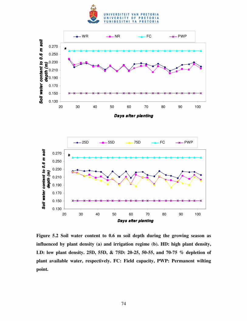
74

0.130

0.150

0.170

0.190

0.210

0.230

0.250

0.270

20 30 40 50 60 70 80 90 100


So

il w

ate

r co

nte

nt

to 0

.6 m

so

il S

oil

wa

ter

con

ten

t to

0.6

m s

oil

So

il w

ate

r co

nte

nt

to 0

.6 m

so

il S

oil

wa

ter

con

ten

t to

0.6

m s

oil

de

pth

(m

)d

ep

th (

m)

de

pth

(m

)d

ep

th (

m)

WR NR FC PWP

aaaa

0.130

0.150

0.170

0.190

0.210

0.230

0.250

0.270

20 30 40 50 60 70 80 90 100


Soi

l w

ater

con

tent

to

0.6

m s

oil

Soi

l w

ater

con

tent

to

0.6

m s

oil

Soi

l w

ater

con

tent

to

0.6

m s

oil

Soi

l w

ater

con

tent

to

0.6

m s

oil

dept

h (m

)de

pth

(m)

dept

h (m

)de

pth

(m)

25D 55D 75D FC PWP

bbbb

Figure 5.2 Soil water content to 0.6 m soil depth during the growing season as

influenced by plant density (a) and irrigation regime (b). HD: high plant density,

LD: low plant density. 25D, 55D, & 75D: 20-25, 50-55, and 70-75 % depletion of

plant available water, respectively. FC: Field capacity, PWP: Permanent wilting

point.

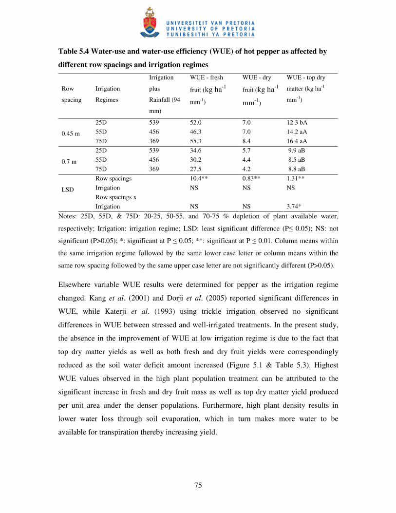
75

Table 5.4 Water-use and water-use efficiency (WUE) of hot pepper as affected by

different row spacings and irrigation regimes

Row

spacing

Irrigation

Regimes

Irrigation

plus

Rainfall (94

mm)

WUE - fresh

fruit (kg ha-1

mm-1)

WUE - dry

fruit (kg ha-1

mm-1)

WUE - top dry

matter (kg ha-1

mm-1)

25D 539 52.0 7.0 12.3 bA 55D 456 46.3 7.0 14.2 aA

0.45 m 75D 369 55.3 8.4 16.4 aA 25D 539 34.6 5.7 9.9 aB 55D 456 30.2 4.4 8.5 aB

0.7 m 75D 369 27.5 4.2 8.8 aB Row spacings 10.4** 0.83** 1.31** Irrigation NS NS NS Row spacings x

LSD

Irrigation NS NS 3.74*


respectively; Irrigation: irrigation regime; LSD: least significant difference (P� 0.05); NS: not

significant (P>0.05); *: significant at P � 0.05; **: significant at P � 0.01. Column means within

the same irrigation regime followed by the same lower case letter or column means within the

same row spacing followed by the same upper case letter are not significantly different (P>0.05).

Elsewhere variable WUE results were determined for pepper as the irrigation regime

changed. Kang et al. (2001) and Dorji et al. (2005) reported significant differences in

WUE, while Katerji et al. (1993) using trickle irrigation observed no significant

differences in WUE between stressed and well-irrigated treatments. In the present study,

the absence in the improvement of WUE at low irrigation regime is due to the fact that

top dry matter yields as well as both fresh and dry fruit yields were correspondingly

reduced as the soil water deficit amount increased (Figure 5.1 & Table 5.3). Highest

WUE values observed in the high plant population treatment can be attributed to the

significant increase in fresh and dry fruit mass as well as top dry matter yield produced

per unit area under the denser populations. Furthermore, high plant density results in

lower water loss through soil evaporation, which in turn makes more water to be

available for transpiration thereby increasing yield.

76

5.4 CONCLUSIONS

This study demonstrated that increased yield could be achieved through frequent

irrigation. For maximum yield, a maximum plant available water depletion level of 20-25

% and a row spacing of 0.45 m are recommended for Long Slim hot pepper. On average,

an irrigation interval of three days was practised to maintain the depletion level of plant

available water between 20-25%. The WUE did not improve by low irrigation regime as

the corresponding yield reduction outweighed the water-saved. The results indicated that

high density planting improved growth and yield per unit area. Yield components like

fruit number, average fruit mass and harvest index were unaffected by row spacing. This

indicates that important yield compensation processes did not occur as the planting

density decreased.

Irrespective of the row spacing used, important parameters like harvest index, leaf

fraction, fresh and dry fruit yields, and fruit number were significantly affected as the

irrigation regime changed, implying that these parameters are not influenced by the

interaction of row spacing and irrigation regime. Therefore, to optimize resource capture

and utilization by hot pepper, an optimum irrigation regime can be determined

independent of the row spacing. Similarly, appropriate row spacing needs to be worked

out, independent of the soil water status, provided that the level of water supply fall

within the current treatment range.

Generally, this study revealed that mild to severe water stress could cause substantial

yield losses in hot pepper, confirming the sensitivity of this crop to water stress.

However, where the cost of fresh water is high, further research is recommended to

establish irrigation regime at soil water depletion level of below 55D. Furthermore,

research that seeks to quantify the trade-off between the yield loss that would be incurred

because of deficit irrigation and the economic and ecological advantage that would be

generated by practicing deficit irrigation is recommended.

77

CHAPTER 6

FAO-TYPE CROP FACTOR DETERMINATION FOR

IRRIGATION SCHEDULING OF HOT PEPPER (Capsicum

annuum L.) CULTIVARS

Abstract

Hot pepper (Capsicum annuum L.) is an irrigated, high value cash crop. Irrigation

requirements can be estimated following a FAO crop factor approach, using information

on basal crop coefficients (Kcb), crop coefficients (Kc) and duration of crop growth

stages. However, this information is lacking for hot pepper cultivars differing in growth

habit and length of growing season under South African conditions. Detailed weather,

soil and crop data were collected from three field trials conducted in the 2004/05 growing

season. A canopy-cover based procedure was used to determine FAO Kcb values and

growth periods for different growth stages. A simple soil water balance equation was

used to estimate the ETc and Kc values of cultivar Long Slim. In addition, initial and

maximum rooting depth and plant heights were determined. A database was generated

containing Kcb and Kc values, growing period duration, rooting depth, and crop height

for different hot pepper cultivars, from which the seasonal water requirements were

determined. The length of different growth stages and the corresponding Kcb values were

cultivar and growing condition dependent. The database can be used to estimate Kcb and

Kc values for new hot pepper cultivars from canopy characteristics. The Soil Water

Balance (SWB) model predicted the soil water deficits to field capacity and fractional

canopy cover well, using the FAO crop factor approach.

Keywords: basal crop coefficient, crop coefficient, crop evapotranspiration, crop model,

SWB model

78

6.1 INTRODUCTION

Hot pepper (Capsicum annuum L.) is a warm season, high value cash crop. Irrigation is

standard practice in hot pepper production (Wein, 1998). Hot pepper cultivars exhibit

considerable biodiversity: cultivars differ vastly in attributes such as growth habit, length

of growing season, cultural requirements, fruit size, pigmentation and pungency

(Bosland, 1992). The water requirements of peppers vary between 600 and 1250 mm per

growth cycle, depending on region, climate and variety (Doorenbos & Kassam, 1979).

Various models, from simple empirical equations to complex and mechanistic models,

are available to estimate plant water requirements by utilizing soil, plant, climatic and

management data. Mechanistic models simulate growth and the canopy size, which

enables the simulation of crop water requirements. However, such models require crop-

specific growth parameters, which are not readily available for all crops and conditions

(Hodges & Ritchie, 1991; Annandale et al., 1999).

The FAO approach was used to develop the irrigation scheduling model CROPWAT

(Smith, 1992) and, in South Africa, SAPWAT (Crosby, 1996; Crosby & Crosby, 1999).

Annandale et al. (1999) also integrated the FAO approach into the Soil Water Balance

(SWB) irrigation scheduling model to simulate water requirements of crops in the

absence of crop-specific growth parameters. Allen et al. (1998) presented an updated

procedure for calculating ETo from daily climatic data, and crop evapotranspiration

(ETc) from ETo and crop coefficients in the FAO 56 report. The FAO 56 report provides

two such crop coefficients, a crop coefficient (Kc) and a basal crop coefficient (Kcb). The

Kc is used to estimate the crop ETc, while the Kcb is used to calculate the potential

transpiration.

The Kc values published in the FAO 56 report represent mean values obtained under

standard growing conditions where limitations on crop growth and evapotranspiration,

due to water shortage, crop density, pests or salinity, are removed. Furthermore, the Kc

values reported by FAO 56 are influenced by the time interval between wetting events,

magnitude of the wetting event, evaporative demand of the atmosphere, and soil type.

Allen et al. (1998) also stressed the need to collect local data on growing seasons and rate

79

of development of irrigated crops to make necessary adjustments to the Kc values to

reflect changes in cultivars and growing conditions.

Since Kcb is a function of crop height and canopy development (Allen et al., 1998), its

value therefore, depends on cultivar, management and climatic conditions (Jagtap &

Jones, 1989; Jovanovic & Annandale, 1999). The Kc and Kcb values for only a few of

the pepper cultivars grown in South Africa are available. The fact that hot pepper is an

irrigated high value cash crop, with wide genetic variability within the species,

necessitated the determination of Kc and Kcb values for local hot pepper cultivars,

representing different growth habits and growing season lengths. Therefore, three field

trials were conducted to determine the seasonal water requirements of hot pepper

cultivars for the area, and to generate a database of Kc and Kcb values, growing periods,

rooting depths, and crop heights for these different hot pepper cultivars. In addition to

the field trials, the SWB model was run using the FAO crop factors generated for cultivar

Long Slim to test the model’s ability to predict soil water deficit and fractional canopy

cover.

80



Detailed weather, soil and crop data were collected from three field trials conducted in

the 2004/2005 growing season at the Hatfield Experimental Farm, University of Pretoria,

Pretoria. The site is located at latitude 25° 45’ S, longitude 28° 16’ E and altitude 1327

m.a.s.l., with an average annual rainfall of 670 mm (Annandale et al., 1999). The average

annual maximum air temperature for the area is 25 °C and the average annual minimum

air temperature is 12 °C. The hottest month of the year is January, with an average

maximum air temperature of 29 °C, while the coldest months are June and July, with an

average minimum air temperature of 5 °C.

The soil physical and chemical properties of the experimental sites are indicated in Table

6.1. Experimental procedures followed are summarized in Table 6.2. In all three

experiments, a plot consisted of five 2.4 m long rows, with an intra-row spacing of 0.4 m.

The two row spacing treatments utilized in both open field and rainshelter experiments

were low plant density (0.7 m) and high plant density (0.45 m). The three irrigation

regime treatments utilized in both open field 1 and rainshelter experiments were high

irrigation (25D: irrigated to field capacity when 20-25% of plant available water was

depleted from the soil), intermediate irrigation (55D: irrigated to field capacity when 50-

55% of plant available water was depleted from the soil), and low irrigation (75D:

irrigated to field capacity when 70-75% of plant available water was depleted from the

soil). Treatments were replicated three times.

6.2.2 Crop management and measurements

Seven-week-old hot pepper seedlings of the respective cultivars were transplanted into

the field. Drip irrigation was used in all three trials. Plants were irrigated for an hour

(12.5 to 15.5 mm) every second day for three weeks until plants were well established.

Thereafter, plants were irrigated to field capacity, every time the predetermined soil water

deficit for each treatment was reached (Table 6.2). Based on soil analysis results and

target yield, 150 kg ha-1 N and 50 kg ha-1 K were applied to all plots. The open field

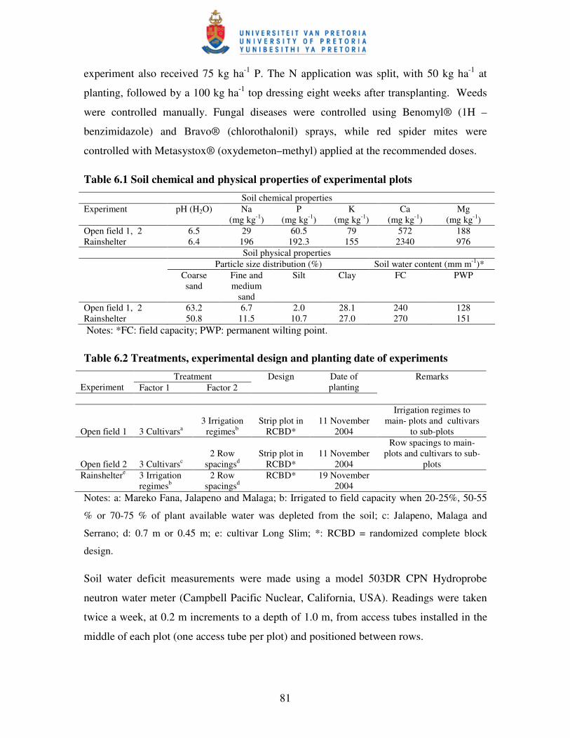
81

experiment also received 75 kg ha-1 P. The N application was split, with 50 kg ha-1 at

planting, followed by a 100 kg ha-1 top dressing eight weeks after transplanting. Weeds

were controlled manually. Fungal diseases were controlled using Benomyl® (1H –

benzimidazole) and Bravo® (chlorothalonil) sprays, while red spider mites were

controlled with Metasystox® (oxydemeton–methyl) applied at the recommended doses.

Table 6.1 Soil chemical and physical properties of experimental plots Soil chemical properties

Experiment pH (H2O) Na (mg kg-1)

P (mg kg-1)

K (mg kg-1)

Ca (mg kg-1)

Mg (mg kg-1)

Open field 1, 2 6.5 29 60.5 79 572 188 Rainshelter 6.4 196 192.3 155 2340 976

Soil physical properties Particle size distribution (%) Soil water content (mm m-1)* Coarse

sand Fine and medium

sand

Silt Clay FC PWP

Open field 1, 2 63.2 6.7 2.0 28.1 240 128 Rainshelter 50.8 11.5 10.7 27.0 270 151 Notes: *FC: field capacity; PWP: permanent wilting point.

Table 6.2 Treatments, experimental design and planting date of experiments Treatment

Experiment Factor 1 Factor 2 Design Date of

planting Remarks

Open field 1

3 Cultivarsa

3 Irrigation

regimesb

Strip plot in

RCBD*

11 November

2004

Irrigation regimes to main- plots and cultivars

to sub-plots Open field 2

3 Cultivarsc

2 Row

spacingsd

Strip plot in

RCBD*

11 November

2004

Row spacings to main- plots and cultivars to sub-

plots Rainsheltere 3 Irrigation

regimesb 2 Row

spacingsd RCBD* 19 November

2004

Notes: a: Mareko Fana, Jalapeno and Malaga; b: Irrigated to field capacity when 20-25%, 50-55

% or 70-75 % of plant available water was depleted from the soil; c: Jalapeno, Malaga and

Serrano; d: 0.7 m or 0.45 m; e: cultivar Long Slim; *: RCBD = randomized complete block

design.

Soil water deficit measurements were made using a model 503DR CPN Hydroprobe

neutron water meter (Campbell Pacific Nuclear, California, USA). Readings were taken

twice a week, at 0.2 m increments to a depth of 1.0 m, from access tubes installed in the

middle of each plot (one access tube per plot) and positioned between rows.

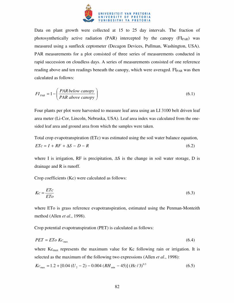
82

Data on plant growth were collected at 15 to 25 day intervals. The fraction of

photosynthetically active radiation (PAR) intercepted by the canopy (FIPAR) was

measured using a sunfleck ceptometer (Decagon Devices, Pullman, Washington, USA).

PAR measurements for a plot consisted of three series of measurements conducted in

rapid succession on cloudless days. A series of measurements consisted of one reference

reading above and ten readings beneath the canopy, which were averaged. FIPAR was then

calculated as follows:

��

��

�−=


FI PAR 1 (6.1)

Four plants per plot were harvested to measure leaf area using an LI 3100 belt driven leaf

area meter (Li-Cor, Lincoln, Nebraska, USA). Leaf area index was calculated from the one-

sided leaf area and ground area from which the samples were taken.




drainage and R is runoff.

Crop coefficients (Kc) were calculated as follows:

EToETc

Kc = (6.3)

where ETo is grass reference evapotranspiration, estimated using the Penman-Monteith

method (Allen et al., 1998).

Crop potential evapotranspiration (PET) is calculated as follows:

maxKcEToPET = (6.4)

where Kcmax represents the maximum value for Kc following rain or irrigation. It is

selected as the maximum of the following two expressions (Allen et al., 1998): 3.0

min2max )3/()]45(004.0)2(04.0[2.1 HcRHUKc −−−+= (6.5)

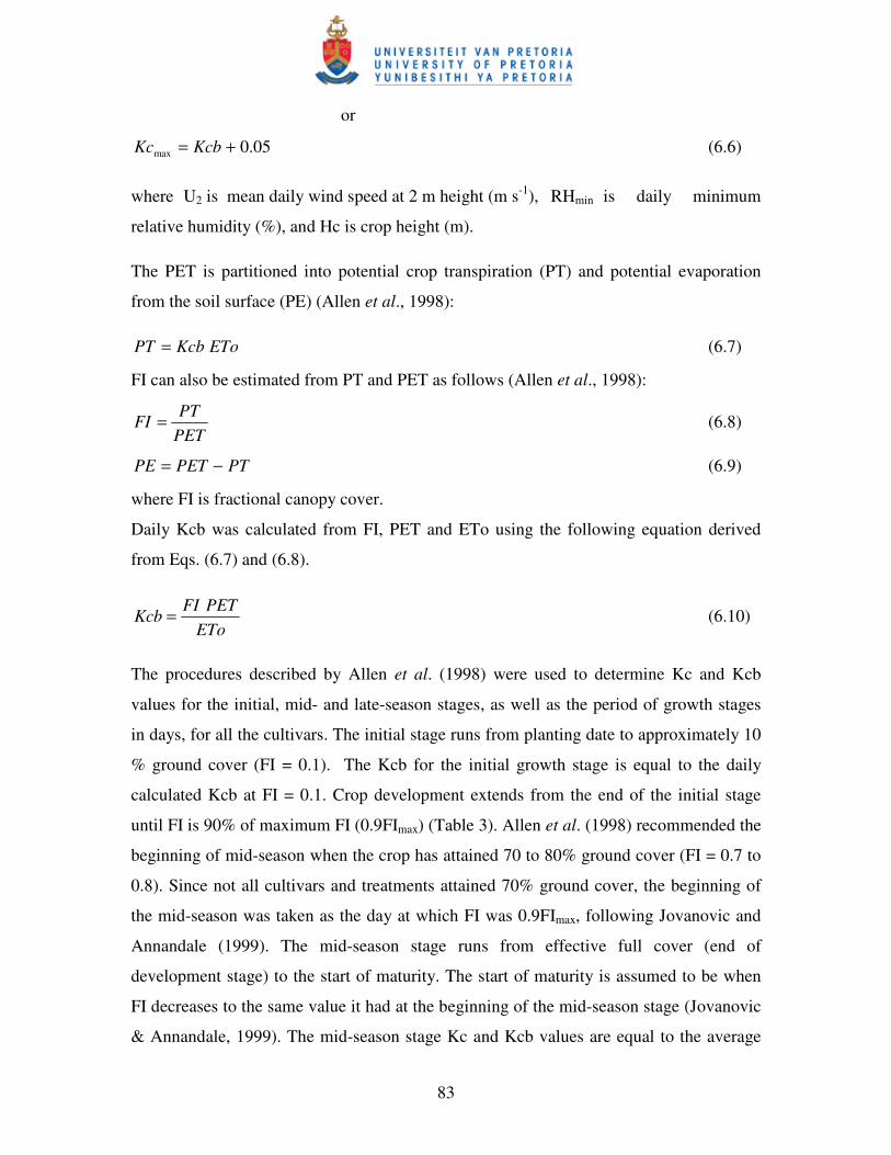
83

or

05.0max += KcbKc (6.6)

where U2 is mean daily wind speed at 2 m height (m s-1), RHmin is daily minimum

relative humidity (%), and Hc is crop height (m).

The PET is partitioned into potential crop transpiration (PT) and potential evaporation

from the soil surface (PE) (Allen et al., 1998):

EToKcbPT = (6.7)

FI can also be estimated from PT and PET as follows (Allen et al., 1998):

PETPT

FI = (6.8)

PTPETPE −= (6.9)

where FI is fractional canopy cover.

Daily Kcb was calculated from FI, PET and ETo using the following equation derived

from Eqs. (6.7) and (6.8).

EToPETFI

Kcb = (6.10)

The procedures described by Allen et al. (1998) were used to determine Kc and Kcb

values for the initial, mid- and late-season stages, as well as the period of growth stages

in days, for all the cultivars. The initial stage runs from planting date to approximately 10

% ground cover (FI = 0.1). The Kcb for the initial growth stage is equal to the daily

calculated Kcb at FI = 0.1. Crop development extends from the end of the initial stage

until FI is 90% of maximum FI (0.9FImax) (Table 3). Allen et al. (1998) recommended the

beginning of mid-season when the crop has attained 70 to 80% ground cover (FI = 0.7 to

0.8). Since not all cultivars and treatments attained 70% ground cover, the beginning of

the mid-season was taken as the day at which FI was 0.9FImax, following Jovanovic and

Annandale (1999). The mid-season stage runs from effective full cover (end of

development stage) to the start of maturity. The start of maturity is assumed to be when

FI decreases to the same value it had at the beginning of the mid-season stage (Jovanovic

& Annandale, 1999). The mid-season stage Kc and Kcb values are equal to the average

84

daily Kc and Kcb values during the mid-season stage. The late-season stage runs from the

end of mid-season stage until the end of the growing season. The late-season stage Kc

and Kcb values are equal to the average daily calculated Kc and Kcb values at the end of

the growing season.

Daily weather data were collected from an automatic weather station located about 100 m

from the experimental site. The automatic weather station consisted of an LI 200X

pyranometer (Li-Cor, Lincoln, Nebraska, USA) to measure solar radiation, an electronic

cup anemometer (MET One, Inc., USA) to measure average wind speed, an electronic

tipping bucket rain gauge (RIMCO, R/TBR, Rauchfuss Instruments Division, Australia),

an ES500 electronic relative humidity and temperature sensor and a CR10X data-logger

(Campbell Scientific, Inc., Logan, Utah, USA).

6.2.3 The Soil Water Balance (SWB) model

The Soil Water Balance (SWB) model is a mechanistic, real-time, user-friendly, generic

crop irrigation scheduling model simulating soil water balance and crop growth from

crop-specific model parameters (Annandale et al., 1999). An FAO approach is embedded

into the SWB irrigation scheduling model to simulate water requirements of crops in the

absence of crop-specific model parameters. The model allows simulation of field soil

water balance, soil water deficit, root depth, fractional canopy cover and crop height and

performs statistical analyses to indicate the level of agreement between simulated and

measured values.

The FAO based subroutine of the SWB model was run for cultivar Long Slim using FAO

crop factors determined from the field experiment and weather data collected. The FAO

based SWB model requires the following input parameters to run the model: basal crop

coefficient values for initial, mid-season and late season stages, crop growth periods in

days and total allowable depletion of soil water (%) for initial, development, mid-season

and late season stages, initial and maximum rooting depth (RD) and plant height (Hc),

potential yield, stress index, maximum transpiration (Tmax), leaf water potential at Tmax

and canopy interception water storage. Furthermore date of planting, irrigation water

amount and weather data are essential to run the model.

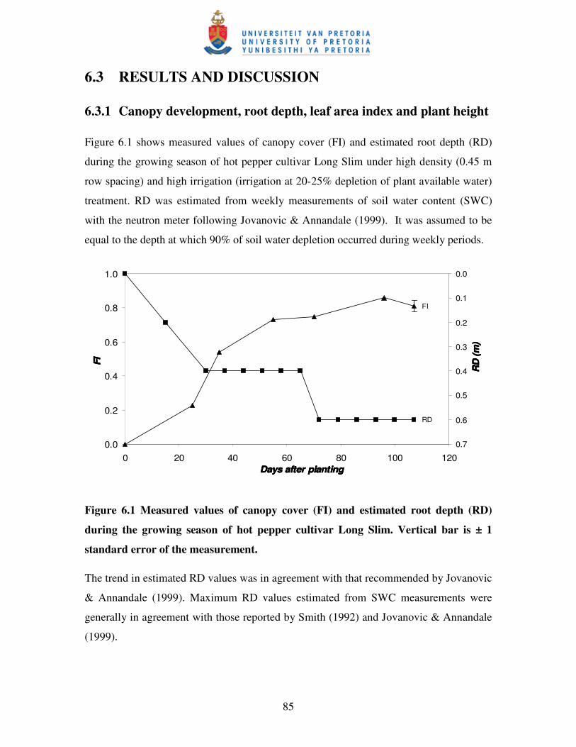
85


6.3.1 Canopy development, root depth, leaf area index and plant height

Figure 6.1 shows measured values of canopy cover (FI) and estimated root depth (RD)

during the growing season of hot pepper cultivar Long Slim under high density (0.45 m

row spacing) and high irrigation (irrigation at 20-25% depletion of plant available water)

treatment. RD was estimated from weekly measurements of soil water content (SWC)

with the neutron meter following Jovanovic & Annandale (1999). It was assumed to be

equal to the depth at which 90% of soil water depletion occurred during weekly periods.

0.0

0.2

0.4

0.6

0.8

1.0

0 20 40 60 80 100 120Days after plantingDays after plantingDays after plantingDays after planting

FIFI FIFI

0.0

0.1

0.2

0.3

0.4

0.5

0.6

0.7

RD

(m

)R

D (

m)

RD

(m

)R

D (

m)

RD

FI

Figure 6.1 Measured values of canopy cover (FI) and estimated root depth (RD)

during the growing season of hot pepper cultivar Long Slim. Vertical bar is ± 1

standard error of the measurement.

The trend in estimated RD values was in agreement with that recommended by Jovanovic

& Annandale (1999). Maximum RD values estimated from SWC measurements were

generally in agreement with those reported by Smith (1992) and Jovanovic & Annandale

(1999).

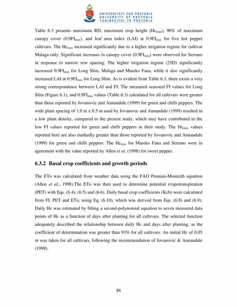
86

Table 6.3 presents maximum RD, maximum crop height (Hcmax), 90% of maximum

canopy cover (0.9FImax), and leaf area index (LAI) at 0.9FImax for five hot pepper

cultivars. The Hcmax increased significantly due to a higher irrigation regime for cultivar

Malaga only. Significant increases in canopy cover (0.9FImax) were observed for Serrano

in response to narrow row spacing. The higher irrigation regime (25D) significantly

increased 0.9FImax for Long Slim, Malaga and Mareko Fana, while it also significantly

increased LAI at 0.9FImax for Long Slim. As is evident from Table 6.3, there exists a very

strong correspondence between LAI and FI. The measured seasonal FI values for Long

Slim (Figure 6.1), and 0.9FImax values (Table 6.3) calculated for all cultivars were greater

than those reported by Jovanovic and Annandale (1999) for green and chilli peppers. The

wide plant spacing of 1.0 m x 0.5 m used by Jovanovic and Annandale (1999) resulted in

a low plant density, compared to the present study, which may have contributed to the

low FI values reported for green and chilli peppers in their study. The Hcmax values

reported here are also markedly greater than those reported by Jovanovic and Annandale

(1999) for green and chilli peppers. The Hcmax for Mareko Fana and Serrano were in

agreement with the value reported by Allen et al. (1998) for sweet pepper.

6.3.2 Basal crop coefficients and growth periods

The ETo was calculated from weather data using the FAO Penman-Monteith equation

(Allen et al., 1998).The ETo was then used to determine potential evapotranspiration

(PET) with Eqs. (6.4), (6.5) and (6.6). Daily basal crop coefficients (Kcb) were calculated

from FI, PET and ETo, using Eq. (6.10), which was derived from Eqs. (6.8) and (6.9).

Daily Hc was estimated by fitting a second-polynomial equation to seven measured data

points of Hc as a function of days after planting for all cultivars. The selected function

adequately described the relationship between daily Hc and days after planting, as the

coefficient of determination was greater than 93% for all cultivars. An initial Hc of 0.05

m was taken for all cultivars, following the recommendation of Jovanovic & Annandale

(1999).

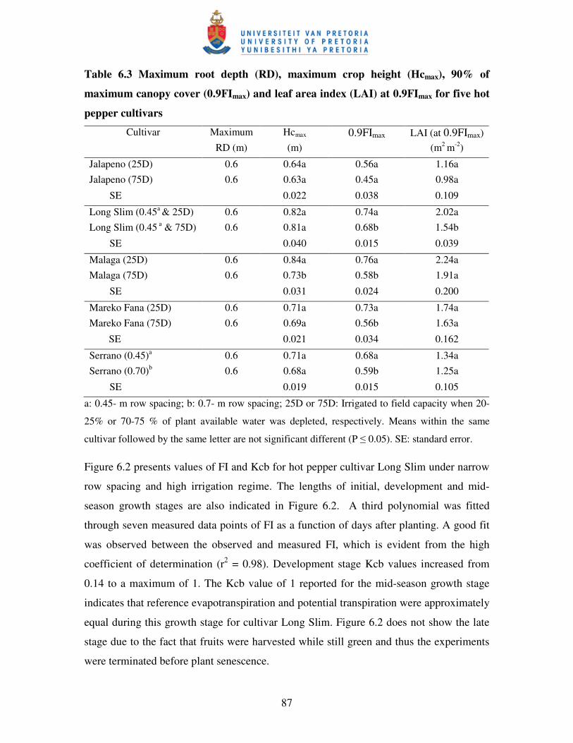
87

Table 6.3 Maximum root depth (RD), maximum crop height (Hcmax), 90% of

maximum canopy cover (0.9FImax) and leaf area index (LAI) at 0.9FImax for five hot

pepper cultivars

Cultivar Maximum Hcmax 0.9FImax LAI (at 0.9FImax) RD (m) (m) (m2 m-2)

Jalapeno (25D) 0.6 0.64a 0.56a 1.16a Jalapeno (75D) 0.6 0.63a 0.45a 0.98a

SE 0.022 0.038 0.109

Long Slim (0.45a & 25D) 0.6 0.82a 0.74a 2.02a Long Slim (0.45 a & 75D) 0.6 0.81a 0.68b 1.54b

SE 0.040 0.015 0.039

Malaga (25D) 0.6 0.84a 0.76a 2.24a Malaga (75D) 0.6 0.73b 0.58b 1.91a

SE 0.031 0.024 0.200

Mareko Fana (25D) 0.6 0.71a 0.73a 1.74a Mareko Fana (75D) 0.6 0.69a 0.56b 1.63a

SE 0.021 0.034 0.162

Serrano (0.45)a 0.6 0.71a 0.68a 1.34a Serrano (0.70)b 0.6 0.68a 0.59b 1.25a

SE 0.019 0.015 0.105

a: 0.45- m row spacing; b: 0.7- m row spacing; 25D or 75D: Irrigated to field capacity when 20-

25% or 70-75 % of plant available water was depleted, respectively. Means within the same

cultivar followed by the same letter are not significant different (P � 0.05). SE: standard error.

Figure 6.2 presents values of FI and Kcb for hot pepper cultivar Long Slim under narrow

row spacing and high irrigation regime. The lengths of initial, development and mid-

season growth stages are also indicated in Figure 6.2. A third polynomial was fitted

through seven measured data points of FI as a function of days after planting. A good fit

was observed between the observed and measured FI, which is evident from the high

coefficient of determination (r2 = 0.98). Development stage Kcb values increased from

0.14 to a maximum of 1. The Kcb value of 1 reported for the mid-season growth stage

indicates that reference evapotranspiration and potential transpiration were approximately

equal during this growth stage for cultivar Long Slim. Figure 6.2 does not show the late

stage due to the fact that fruits were harvested while still green and thus the experiments

were terminated before plant senescence.

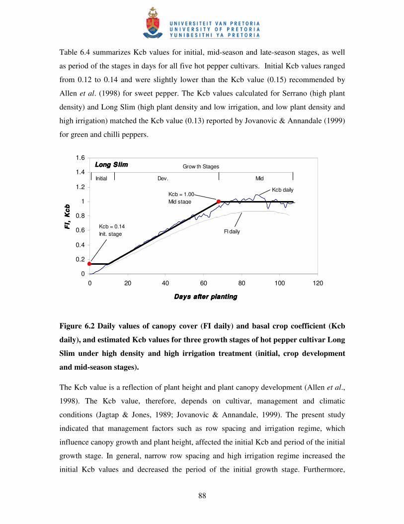
88

Table 6.4 summarizes Kcb values for initial, mid-season and late-season stages, as well

as period of the stages in days for all five hot pepper cultivars. Initial Kcb values ranged

from 0.12 to 0.14 and were slightly lower than the Kcb value (0.15) recommended by

Allen et al. (1998) for sweet pepper. The Kcb values calculated for Serrano (high plant

density) and Long Slim (high plant density and low irrigation, and low plant density and

high irrigation) matched the Kcb value (0.13) reported by Jovanovic & Annandale (1999)

for green and chilli peppers.

Long SlimLong SlimLong SlimLong Slim

0

0.2

0.4

0.6

0.8

1

1.2

1.4

1.6

0 20 40 60 80 100 120


FI,

Kcb

FI,

Kcb

FI,

Kcb

FI,

Kcb

Kcb = 0.14Init. stage

Kcb = 1.00Mid stage

Kcb daily

Initial Dev. Mid

Grow th Stages

FI daily

Figure 6.2 Daily values of canopy cover (FI daily) and basal crop coefficient (Kcb

daily), and estimated Kcb values for three growth stages of hot pepper cultivar Long

Slim under high density and high irrigation treatment (initial, crop development

and mid-season stages).

The Kcb value is a reflection of plant height and plant canopy development (Allen et al.,

1998). The Kcb value, therefore, depends on cultivar, management and climatic

conditions (Jagtap & Jones, 1989; Jovanovic & Annandale, 1999). The present study

indicated that management factors such as row spacing and irrigation regime, which

influence canopy growth and plant height, affected the initial Kcb and period of the initial

growth stage. In general, narrow row spacing and high irrigation regime increased the

initial Kcb values and decreased the period of the initial growth stage. Furthermore,

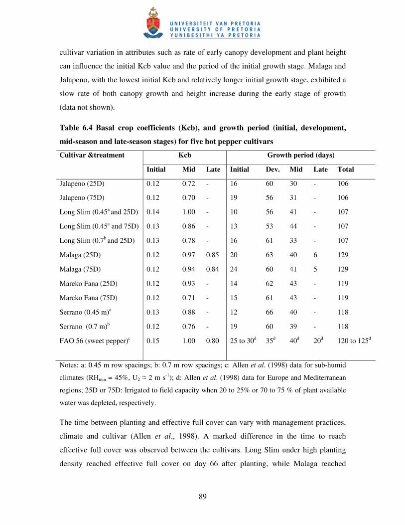
89

cultivar variation in attributes such as rate of early canopy development and plant height

can influence the initial Kcb value and the period of the initial growth stage. Malaga and

Jalapeno, with the lowest initial Kcb and relatively longer initial growth stage, exhibited a

slow rate of both canopy growth and height increase during the early stage of growth

(data not shown).

Table 6.4 Basal crop coefficients (Kcb), and growth period (initial, development,

mid-season and late-season stages) for five hot pepper cultivars

Kcb Growth period (days) Cultivar &treatment

Initial Mid Late Initial Dev. Mid Late Total

Jalapeno (25D) 0.12 0.72 - 16 60 30 - 106

Jalapeno (75D) 0.12 0.70 - 19 56 31 - 106

Long Slim (0.45a and 25D) 0.14 1.00 - 10 56 41 - 107

Long Slim (0.45a and 75D) 0.13 0.86 - 13 53 44 - 107

Long Slim (0.7b and 25D) 0.13 0.78 - 16 61 33 - 107

Malaga (25D) 0.12 0.97 0.85 20 63 40 6 129

Malaga (75D) 0.12 0.94 0.84 24 60 41 5 129

Mareko Fana (25D) 0.12 0.93 - 14 62 43 - 119

Mareko Fana (75D) 0.12 0.71 - 15 61 43 - 119

Serrano (0.45 m)a 0.13 0.88 - 12 66 40 - 118

Serrano (0.7 m)b 0.12 0.76 - 19 60 39 - 118

FAO 56 (sweet pepper)c 0.15 1.00 0.80 25 to 30d 35d 40d 20d 120 to 125d

Notes: a: 0.45 m row spacings; b: 0.7 m row spacings; c: Allen et al. (1998) data for sub-humid

climates (RHmin = 45%, U2 � 2 m s-1); d: Allen et al. (1998) data for Europe and Mediterranean

regions; 25D or 75D: Irrigated to field capacity when 20 to 25% or 70 to 75 % of plant available

water was depleted, respectively.

The time between planting and effective full cover can vary with management practices,

climate and cultivar (Allen et al., 1998). A marked difference in the time to reach

effective full cover was observed between the cultivars. Long Slim under high planting

density reached effective full cover on day 66 after planting, while Malaga reached

90

effective full cover on day 83 after planting. It appears that although differences were

small, high density planting and high irrigation regime tended to shorten the time

between planting and effective full cover.

Mid-season Kcb values for all cultivars and treatments ranged between 0.70 and 1. Long

Slim under high density planting gave a mid-season Kcb value of 1, and Malaga under

both high and low planting density, and Mareko Fana under high irrigation regime gave

mid-season Kcb values close to 1, which is the FAO’s recommended Kcb value for sweet

pepper. However, cultivars Jalapeno, Mareko Fana, Serrano and Long Slim under low

irrigation regime and/or low density planting gave mid-season Kcb values lower than 0.9.

All the cultivars and treatments produced mid-season Kcb values that are markedly

higher than mid-season Kcb values reported by Jovanovic & Annandale (1999) for chilli

and green peppers. This is because all the cultivars included in the present study have a

long growing season with prolific canopy growth compared to those cultivars used by

Jovanovic & Annandale (1999). High density planting and early November planting, in

the present study, also may have contributed to higher Kcb values.

In all cultivars and treatments, the duration of the development stage was longer than that

of the mid-season stage, which is in agreement with results reported by Jovanovic &

Annandale (1999). However, Allen et al. (1998) reported that the duration of the mid-

season stage is longer than the development stage for sweet pepper. The variation can be

attributed to the differences in criteria used to mark the end of the developmental stage.

Allen et al. (1998) assumed the beginning of the mid-season when the crop has attained

70 to 80% ground cover (FI = 0.7 to 0.8). In the present study and that of Jovanovic &

Annandale (1999), the end of the development stage was marked when the crop attained

an FI value of 90% of maximum FI, since peppers did not reach FI values of 0.7 to 0.8.

No cultivar, except Malaga, reached the end of mid-season, according to the set criterion,

due to the fact that fruits were harvested while green and thus the experiments were

terminated before plant senescence. The late-season Kcb value Malaga was greater than

0.8, and similar to the late-season Kcb value recommended for sweet pepper by Allen et

al. (1998). The purpose for which the produce is harvested (green pepper versus red

91

pepper) dictates the time of harvest. This directly dictates the length of the late-season

stage and hence the late season Kcb value, as Kcb values decrease linearly from the end

of mid-season to the end of the late season growth stages. The present late season Kcb

value is the average value for 6 days during the late season, as opposed to the Kcb value

reported by Allen et al. (1998) which is the average value of 20 days during the late

season.

New cultivars are released regularly due to market demand and the broad genetic basis of

the species. This makes it important to predict FAO-type crop factors that would likely fit

new cultivars. Table 6.5 and Figure 6.3 present some morphological characteristics of the

five cultivars considered in the experiments. Understanding features of these cultivars

and their corresponding FAO-type crop factors can aid in estimating Kcb values for

newly released cultivars. Generally, cultivars with high FI, LAI and/or Hcmax values gave

relatively greater Kcb values as compared to cultivars with relatively low FI, LAI and/or

Hcmax values. Furthermore, high density planting and high irrigation regime appeared to

increase Kcb values. Accordingly, a newly released cultivar of short to medium height

and small to medium canopy size, similar to cultivars Jalapeno, Long Slim and Serrano,

can have mid-season Kcb values of 0.7 to 0.9 under optimum soil water regime and/or

high planting density. Similarly, cultivars with medium to tall plant height and medium to

large canopy size, similar to cultivars Malaga and Mareko Fana, can be assigned a mid-

season Kcb value of 0.9 to 1 under optimum soil water regime and/or high planting

density. If either deficit irrigation and/or low density planting are intended, the mid-

season Kcb values need to be reduced by at least 0.1. Generally, initial season Kcb values

of 0.12 to 0.14 appear to be acceptable for hot pepper cultivars (depending on the initial

canopy size).

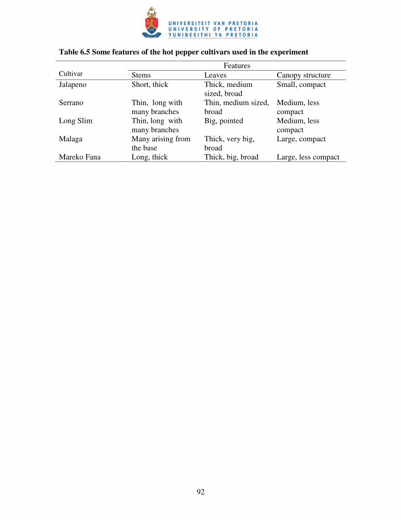
92

Table 6.5 Some features of the hot pepper cultivars used in the experiment

Features Cultivar Stems Leaves Canopy structure Jalapeno Short, thick Thick, medium

sized, broad Small, compact

Serrano Thin, long with many branches

Thin, medium sized, broad

Medium, less compact

Long Slim Thin, long with many branches

Big, pointed Medium, less compact

Malaga Many arising from the base

Thick, very big, broad

Large, compact

Mareko Fana Long, thick Thick, big, broad Large, less compact

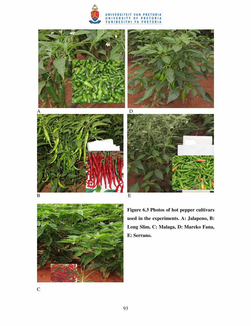
93

A D

B E

Figure 6.3 Photos of hot pepper cultivars

used in the experiments. A: Jalapeno, B:

Long Slim, C: Malaga, D: Mareko Fana,

E: Serrano.

C

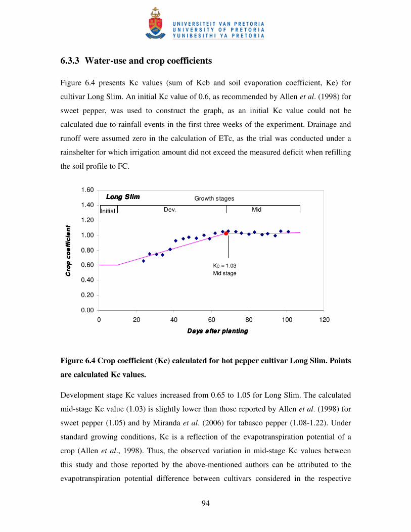
94

6.3.3 Water-use and crop coefficients

Figure 6.4 presents Kc values (sum of Kcb and soil evaporation coefficient, Ke) for

cultivar Long Slim. An initial Kc value of 0.6, as recommended by Allen et al. (1998) for

sweet pepper, was used to construct the graph, as an initial Kc value could not be

calculated due to rainfall events in the first three weeks of the experiment. Drainage and

runoff were assumed zero in the calculation of ETc, as the trial was conducted under a

rainshelter for which irrigation amount did not exceed the measured deficit when refilling

the soil profile to FC.

Long SlimLong SlimLong SlimLong Slim

0.00

0.20

0.40

0.60

0.80

1.00

1.20

1.40

1.60

0 20 40 60 80 100 120


Cro

p c

oe

ffic

ien

tC

rop

co

eff

icie

nt

Cro

p c

oe

ffic

ien

tC

rop

co

eff

icie

nt

Kc = 1.03Mid stage

Initial Dev. Mid

Growth stages

Figure 6.4 Crop coefficient (Kc) calculated for hot pepper cultivar Long Slim. Points

are calculated Kc values.

Development stage Kc values increased from 0.65 to 1.05 for Long Slim. The calculated

mid-stage Kc value (1.03) is slightly lower than those reported by Allen et al. (1998) for

sweet pepper (1.05) and by Miranda et al. (2006) for tabasco pepper (1.08-1.22). Under

standard growing conditions, Kc is a reflection of the evapotranspiration potential of a

crop (Allen et al., 1998). Thus, the observed variation in mid-stage Kc values between

this study and those reported by the above-mentioned authors can be attributed to the

evapotranspiration potential difference between cultivars considered in the respective

95

studies. Furthermore, climatic conditions under which the experiments were conducted

dictate the reference evapotranspiration and evapotranspiration potential, which are the

two variables determining Kc.

Table 6.6 presents the soil water storage, simulated seasonal soil evaporation (Esim), crop

transpiration (Tsim) and evapotranspiration (ETsim) for various cultivars. The measured

evapotranspiration (ETmeas) for Long Slim is also shown. These values were determined

under optimum growing conditions (high irrigation, high plant density, or a combination

of the two). The negative �S values indicate a loss in soil water storage.

Evapotranspiration (ETmeas) was measured only for Long Slim, as this experiment was

conducted in a rainshelter. Evapotranspiration for the remaining four cultivars could not

be measured accurately due to high rainfall interference during the growing season.

Hence, it was not possible to apply the soil water balance equation (Jovanovic &

Annandale, 1999), as runoff and drainage could not be measured.

The cumulative potential evapotranspiration calculated (PET) in a given environment is a

function of plant height and length of growing season (Allen et al., 1998). In the present

study, ETsim for all cultivars ranged between 390 and 546 mm. The total ETsim deviated

by 30 mm from the ETmeas for cultivar Long Slim. All evapotranspiration values reported

here fall outside the range reported by Doorenbos & Kassam (1979) for pepper, which

varies from 600 to 1250 mm, depending on the region, climate and cultivar. Growing

conditions, climate and cultivar differences may have contributed to the observed

differences between the present results and those of Doorenbos & Kassam (1979).

Furthermore, water lost through drainage and canopy interception was not accounted in

this study, which might have contributed to the relatively low ET values reported here.

On the contrary, seasonal evapotranspiration reported by Jovanovic & Annandale (1999)

were lower than those obtained in this study, as cultivars considered in the two studies

differed in the total length of the growing season and canopy size.

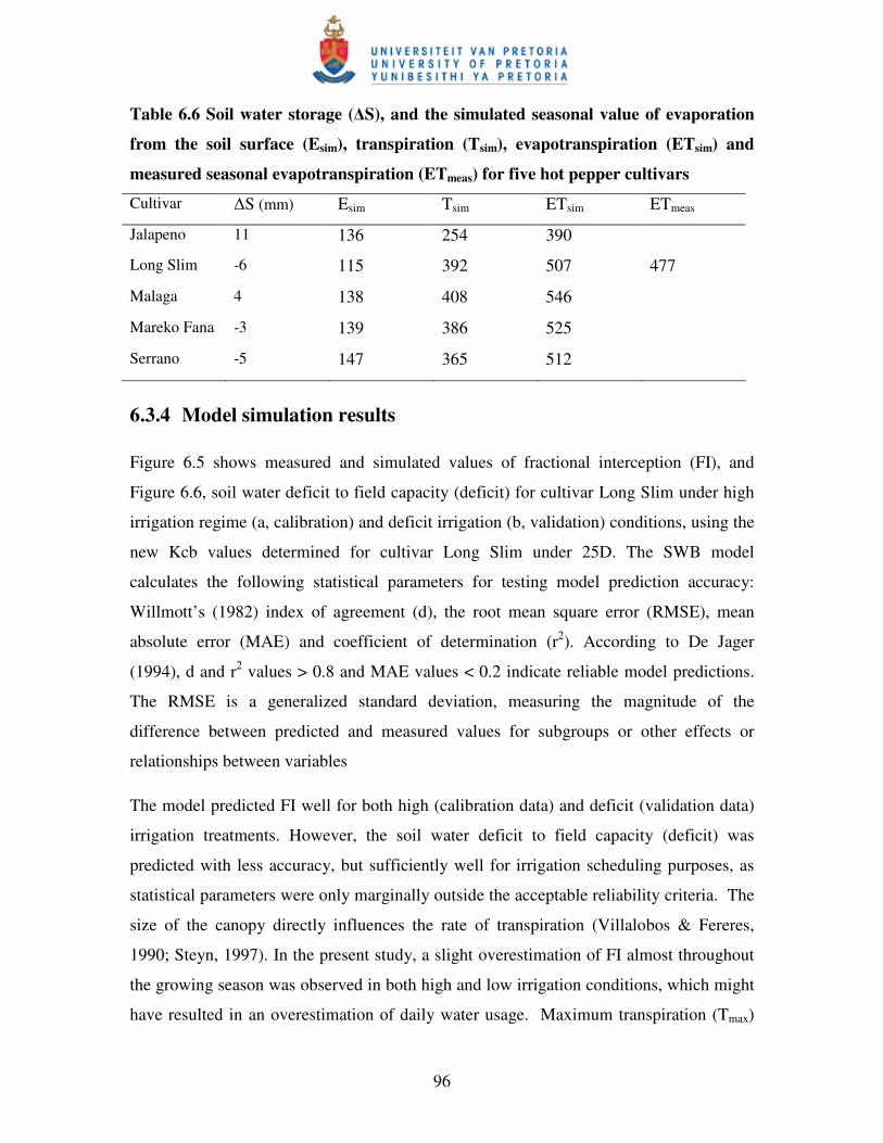
96

Table 6.6 Soil water storage (�S), and the simulated seasonal value of evaporation

from the soil surface (Esim), transpiration (Tsim), evapotranspiration (ETsim) and

measured seasonal evapotranspiration (ETmeas) for five hot pepper cultivars

Cultivar �S (mm) Esim Tsim ETsim ETmeas

Jalapeno 11 136 254 390

Long Slim -6 115 392 507 477

Malaga 4 138 408 546

Mareko Fana -3 139 386 525

Serrano -5 147 365 512

6.3.4 Model simulation results

Figure 6.5 shows measured and simulated values of fractional interception (FI), and

Figure 6.6, soil water deficit to field capacity (deficit) for cultivar Long Slim under high

irrigation regime (a, calibration) and deficit irrigation (b, validation) conditions, using the

new Kcb values determined for cultivar Long Slim under 25D. The SWB model

calculates the following statistical parameters for testing model prediction accuracy:

Willmott’s (1982) index of agreement (d), the root mean square error (RMSE), mean

absolute error (MAE) and coefficient of determination (r2). According to De Jager

(1994), d and r2 values > 0.8 and MAE values < 0.2 indicate reliable model predictions.

The RMSE is a generalized standard deviation, measuring the magnitude of the

difference between predicted and measured values for subgroups or other effects or

relationships between variables

The model predicted FI well for both high (calibration data) and deficit (validation data)

irrigation treatments. However, the soil water deficit to field capacity (deficit) was

predicted with less accuracy, but sufficiently well for irrigation scheduling purposes, as

statistical parameters were only marginally outside the acceptable reliability criteria. The

size of the canopy directly influences the rate of transpiration (Villalobos & Fereres,

1990; Steyn, 1997). In the present study, a slight overestimation of FI almost throughout

the growing season was observed in both high and low irrigation conditions, which might

have resulted in an overestimation of daily water usage. Maximum transpiration (Tmax)

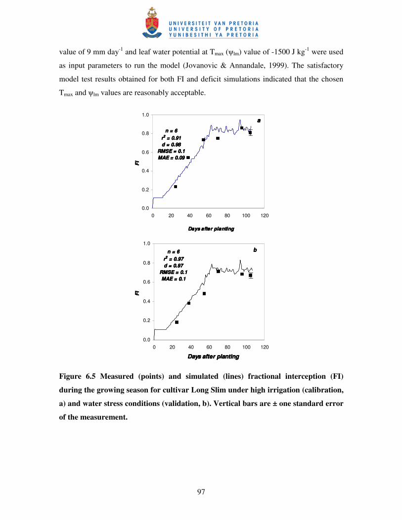
97

value of 9 mm day-1 and leaf water potential at Tmax (�lm) value of -1500 J kg-1 were used

as input parameters to run the model (Jovanovic & Annandale, 1999). The satisfactory

model test results obtained for both FI and deficit simulations indicated that the chosen

Tmax and �lm values are reasonably acceptable.

n = 6n = 6n = 6n = 6rrrr2222 = 0.91 = 0.91 = 0.91 = 0.91d = 0.98d = 0.98d = 0.98d = 0.98

RMSE = 0.1RMSE = 0.1RMSE = 0.1RMSE = 0.1MAE = 0.09MAE = 0.09MAE = 0.09MAE = 0.09

0.0

0.2

0.4

0.6

0.8

1.0

0 20 40 60 80 100 120


FI

FI

FI

FI

aaaa

n = 6n = 6n = 6n = 6rrrr2222 = 0.97 = 0.97 = 0.97 = 0.97d = 0.97d = 0.97d = 0.97d = 0.97


0.0

0.2

0.4

0.6

0.8

1.0

0 20 40 60 80 100 120


FI

FI

FI

FI

bbbb

Figure 6.5 Measured (points) and simulated (lines) fractional interception (FI)

during the growing season for cultivar Long Slim under high irrigation (calibration,

a) and water stress conditions (validation, b). Vertical bars are ± one standard error

of the measurement.

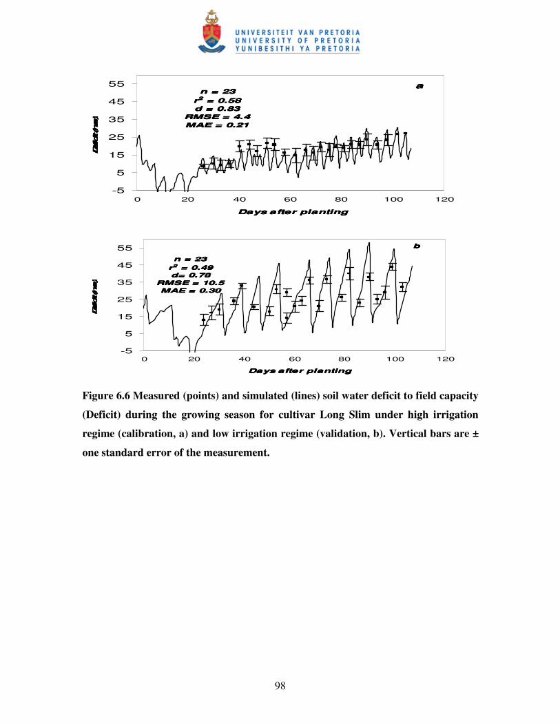
98

n = 23n = 23n = 23n = 23rrrr2222 = 0.58 = 0.58 = 0.58 = 0.58d = 0.83d = 0.83d = 0.83d = 0.83


-5

5

15

25

35

45

55

0 20 40 60 80 100 120


Deficit (m

m)

Deficit (m

m)

Deficit (m

m)

Deficit (m

m)

aaaa

n = 23n = 23n = 23n = 23rrrr2222 = 0.49 = 0.49 = 0.49 = 0.49d= 0.78d= 0.78d= 0.78d= 0.78


-5

5

15

25

35

45

55

0 20 40 60 80 100 120


Deficit (m

m)

Deficit (m

m)

Deficit (m

m)

Deficit (m

m)

bbbb

Figure 6.6 Measured (points) and simulated (lines) soil water deficit to field capacity

(Deficit) during the growing season for cultivar Long Slim under high irrigation

regime (calibration, a) and low irrigation regime (validation, b). Vertical bars are ±

one standard error of the measurement.

99

6.4 CONCLUSIONS

A database of basal crop coefficients and growth periods were determined for five hot

pepper cultivars, using weather data and plant parameters such as plant height and canopy

cover. A simple procedure that utilizes canopy cover was followed to mark the beginning

and end of the different growth stages and determine their Kcb values.

The duration of different growth stages and their corresponding Kcb values were cultivar

and growing condition dependent. These results can be useful for estimating Kcb values

of newly released hot pepper cultivars, based on their growth patterns. A new cultivar of

short to medium height and small to medium canopy size can have a mid-season Kcb

value of 0.7 to 0.8 under an optimum soil water regime and/or high planting density

conditions. Similarly, cultivars of medium to tall height and medium to large canopy size

can be assigned a mid-season Kcb value of 0.9 to 1 under good soil water supply

conditions and/or high planting density. If either deficit irrigation and/or low density

planting are intended, the mid-season Kcb values need to be reduced by at least 0.1.

Generally, initial season Kcb values ranging from 0.12 to 0.14 appears to be acceptable

for most hot pepper cultivars (depending on the initial canopy size).

A crop coefficient value of 1.03 for the mid-season stage and seasonal evapotranspiration

of 577 mm were estimated for cultivar Long Slim. Evapotranspiration simulated across

cultivars ranged from 390 to 546 mm. Simulation results showed that the simple FAO

crop factor based model, which is embedded in the SWB model, could reasonably well

simulate FI and the soil water deficits to field capacity.

100

CHAPTER 7

SWB PARAMETER DETERMINATION AND STABILITY

ANALYSIS UNDER DIFFERENT IRRIGATION REGIMES

AND ROW SPACINGS IN HOT PEPPER (Capsicum annuum

L.) CULTIVARS

Abstract

Hot pepper (Capsicum anunum L.) is an irrigated and high value cash crop. Irrigation can

be scheduled with crop models, such as SWB. Since SWB is a generic crop model,

determination of crop-specific model parameters for each crop is required to schedule

irrigation. Ascertaining stability of crop-specific model parameters across cultivars and

different growing conditions helps to ensure transferability of parameters. The objective

of this study was to determine crop-specific model parameters for five hot pepper

cultivars and to analyse the stability of these parameters across the five cultivars, three

irrigation regimes and two row spacings. Detailed weather, soil and crop data were

collected from three field trials conducted in the 2004/05 growing season at the Hatfield

Experimental Farm, University of Pretoria and used to generate a database of model

parameters. These include canopy radiation extinction coefficient, radiation use

efficiency, specific leaf area, leaf-stem partitioning parameter, vapour pressure-corrected

dry matter/water ratio and thermal time requirements for developmental stages.

Almost all crop-specific model parameters studied appeared to remain stable under

different irrigation regimes and row spacings. However, marked differences in almost all

crop-specific model parameters were observed due to cultivar differences in canopy

structure, size and dry matter production. Therefore, the investigated crop-specific model

parameters should be transferable to simulate growth and irrigation scheduling over

different irrigation regimes and row spacings within a specific cultivar. Crop-specific

101

model parameters for new hot pepper cultivars may be estimated from this database,

using canopy characteristics, day degrees to maturity and dry matter production potential.

Keywords: crop growth modelling, crop parameter, hot pepper, irrigation scheduling,

SWB model

102

7.1 INTRODUCTION

Hot pepper (Capsicum annuum L.) is a warm season, high value cash crop. Irrigation is

standard practice in hot pepper production (Wein, 1998). Both under- and over-irrigation

can be detrimental to the profitability of crops. Under-irrigation will result in yield and

quality reduction, while over-irrigation can lead to a rise in the water table, leaching of

agro-chemicals to groundwater and accumulation of salt on the soil surface, which have

damaging environmental impacts and waste water, energy and nutrients.

One avenue of increasing water-use efficiency and protecting the environmental against

degradation is the adoption of irrigation scheduling. Various techniques and instruments

are available for irrigation scheduling. Quantifying soil water or plant water status using

different instruments can give an idea of how much and when to irrigate (Jones, 2004).

Nevertheless, an approach that takes into account the soil-plant-atmosphere continuum in

determining the water requirement of a crop is more realistic in predicting its water

requirements (Annandale et al., 1999). Nowadays models are often utilized for this

purpose.

Various models, from simple empirical equations to complex dynamic mechanistic

simulators, are available to estimate plant water requirements, using soil, plant, climatic

and management data (Smith, 1992; Sinclair & Seligman, 1996). Mechanistic models

usually grow the canopy to simulate water requirements; however, such models require

crop-specific model parameters, which are not readily available for all crops and

conditions (Hodges & Ritchie, 1991; Annandale et al., 1999). One such model is the Soil

Water Balance (SWB) model (Annandale et al., 1999). The SWB is a mechanistic, user-

friendly, daily time step, generic crop irrigation scheduling model. It is capable of

simulating yield, different growth processes, and field water balance components.

As SWB is a generic crop model, determination of crop-specific model parameters for

each crop is crucial to simulate growth and schedule irrigations. Crop-specific model

parameters are the reflection of a cultivar’s canopy characteristics, day degrees to

different phenological stages and potential dry matter production, which in turn are

affected by a cultivar’s genotype and growing conditions. For instance, crop-specific

103

model parameters were shown to differ across cultivars (Kiniry et al., 1989; Annandale et

al., 1999), vapour pressure deficit differences (Tanner & Sinclair, 1983; Stockle &

Kiniry, 1990), irrigation frequencies (Tesfaye et al., 2006), row spacings (Flénet et al.,

1996; Jovanovic et al., 2002) and other growing conditions (Monteith, 1994; Sinclair &

Muchow, 1999).

Hot pepper cultivars exhibit considerable biodiversity: cultivars differ vastly in attributes

such as growth habit, length of growing season, cultural requirements, fruit size,

pigmentation and pungency (Bosland, 1992). Therefore, there is a need to determine

crop-specific model parameters for a particular cultivar and to ascertain stability of these

parameters under different growing conditions. The objective of this study was to

determine SWB crop-specific model parameters of five hot pepper cultivars differing in

growth habit and length of growing season. A further objective was to analyze stability of

the parameters across five cultivars, three irrigation regimes and two row spacings.

104



Details of the site and treatments are provided in paragraph 6.2.1 of Chapter 6.



dripping laid fields. Plants were irrigated for 1 hour (12.5-15.5 mm) every other day for

three weeks until plants were well established. Thereafter, plants were irrigated to field

capacity, each time the predetermined soil water deficit was reached, according to the

treatment. In the open field 2 experiment, the plots were irrigated to field capacity when

50-55 % of plant available water was depleted. Irrigation was scheduled using soil water

deficit measurements made using a model 503DR CPN Hydroprobe neutron water meter

(Campbell Pacific Nuclear, California, USA). Readings were taken twice a week, at 0.2

m increments to a depth of 1.0 m, from access tubes installed in the middle of each plot

and positioned between rows.

Based on soil analysis results and target yields, 150 kg ha-1 N and 50 kg ha-1 K were

applied to all experiments. The open field experiments, however, also received 75 kg ha-1

P. The N application was split, with 50 kg ha-1 applied at planting, followed by a 100 kg

ha-1 top dressing eight weeks after transplanting. Weeds were controlled manually.

Preventative spraying for fungal diseases was done using Benomyl ® (1H –

benzoimidazole) and Bravo ® (chlorothalonil), while red spider mites were controlled

with Metasystox ® (oxydemeton–methyl).

The fraction of photosynthetically active radiation (PAR) intercepted by the canopy

(FIPAR) was measured using a sunfleck ceptometer (Decagon Devices, Pullman,

Washington, USA). The PAR measurements for a plot consisted of three series of

measurements conducted in rapid succession on cloudless days. A series of

measurements consisted of one reference reading above and ten readings beneath the

canopy, which were averaged. FIPAR was then calculated as follows:

105

��

��

�−=


FI PAR 1 (7.1)

Growth analyses were carried out at 15 to 25 day intervals by harvesting four plants from

each plot. The sampled plants were separated into leaves, stems and fruits. Leaf area was

measured with an LI 3100 belt driven leaf area meter (Li-Cor, Lincoln, Nebraska, USA).

Samples were then oven dried to a constant mass and weighed.








7.2.3 Crop-specific model parameters determination and data analysis

Weather and growth analysis data were used to determine crop-specific model

parameters. These included canopy radiation extinction coefficient, radiation use

efficiency, specific leaf area, leaf-stem partitioning parameter, vapour pressure-corrected

dry matter/water ratio and thermal time requirements for developmental stages

(Jovanovic et al., 1999).

The canopy radiation extinction coefficient for PAR (KPAR) was determined using a basic

equation describing transmission of solar radiation through the plant canopy, which is

similar to Bouguer’s law (Campbell & Van Evert, 1994):

( )LAIKFI PARPAR −−= exp1 (7.2)

where FIPAR is fractional interception of PAR, and LAI is leaf area index (m2 m-2).

The light extinction coefficient for solar radiation (Ks ) is used by SWB to predict

radiation-limited dry matter production (Monteith, 1977) and for partitioning

evapotranspiration into evaporation from the soil surface and crop transpiration (Ritchie,

106

1972). The KPAR was converted to Ks following procedures recommended by Campbell

and Van Evert (1994).

sbds aKK = (7.3)

pPARbd aKK = (7.4)

nps aaa = (7.5)

where Kbd is canopy radiation extinction coefficient for ‘black’ leaves which diffuse

radiation, as is leaf absorptance of solar radiation, ap is leaf absorptance of PAR, and an is

leaf absorptance of near infrared radiation (NIR, 0.7-3 �m). The value of ap was assumed

to be 0.8, while an was assumed to be 0.2 (Goudriaan, 1977).

Radiation use efficiency (Ec, g MJ-1) is determined based on a linear relationship

established by Monteith (1977) between accumulated crop dry matter and intercepted

solar radiation, which is:

ssc RFIEDM εε = (7.6)

where DM is dry matter production (g m-2), FIs is fractional interception for total solar

radiation, and Rs is daily total incident solar radiation (MJ m-2). FIs was determined by

using Eq. (7.2), by substituting Ks in place of KPAR. The Ec was determined by fitting a

linear regression equation between cumulative biomass production and cumulative Rs

interception. The slope of the regression line forced through the origin represents Ec.

The leaf-stem partitioning parameter was determined as a function of SLA, LAI and

CDM, by combining Eqs. (7.7) through (7.9) (Jovanovic et al., 1999). The slope of the

regression line represents the leaf-stem partitioning parameter in m2 kg-1.

)1/( CDMpCDMLDM += (7.7)

SDMLDMCDM += (7.8)

LDM is used to calculate LAI as follows:

LDMSLALAI = (7.9)

107

where LDM is leaf dry matter (kg m-2), CDM is canopy dry matter (kg m-2), SDM is

stem dry matter (kg m-2), LAI is leaf area index (m2 m-2) and SLA is the specific leaf area

in m2 kg-1.

Vapour pressure deficit-corrected dry matter/water ratio (DWR) of five hot pepper

cultivars was calculated following Tanner & Sinclair (1983):

( ) PTVPDDMDWR /= (7.10)

where DM (kg m-2) is above-ground biomass, and was measured at harvest, whilst VPD

represents the seasonal average vapour pressure deficit. Both VPD and DWR are in

Pascal (Pa). PT (mm) is potential transpiration and was calculated from potential

evapotranspiration and canopy cover following Allen et al. (1998). Daily VPD calculated

from measurements of maximum air temperature (Tamax), minimum air temperature

(Tamin), maximum relative humidity (RHmax) and minimum relative humidity (RHmin)

adopting the following procedure recommended by the FAO 56 report (Allen et al.,

1998):

asTasTa e

eeVPD −�

�

��

� +=2

minmax (7.11)

where EsTamax is saturated vapour pressure at maximum air temperature (kPa), EsTamin is

saturated vapour pressure at minimum air temperature (kPa) and ea is actual vapour

pressure (kPa).

Saturated vapour pressure (es) at maximum (Tamax) and minimum air temperature (Tamin)

was calculated by replacing T with Tamax and Tamin (°C) in the following equation (Allen

et al., 1998):

��

�

�

+=

3.23727.17

exp6108.0T

Tes (7.12)

ea was calculated from measured daily Tamax, Tamin, RHmax and RHmin using the following

equation (Allen et al., 1998):

2100

)(100

)( minmax

maxmin

RHTe

RHTe

ess

a

+= (7.13)

108

Growing day degree (GDD) (d °C) was determined from daily average air temperature

(Tavg) following Monteith (1977):

( ) tTTGDD bavg ∆−= (7.14)

where Tb is the temperature (°C) below which development is assumed to cease and �t is

the time step (one day). The Tb value recommended by Knott (1988) (11 °C) was used in

this study.

The calculated crop-specific model parameters were analyzed using SAS statistically

software version 9.1 (SAS, 2003) to see if there was significant statistical differences due

to treatment effects. When a significant difference was observed due to a treatment, the

F-test was conducted using SAS statistical software to separate means at P = 0.05.

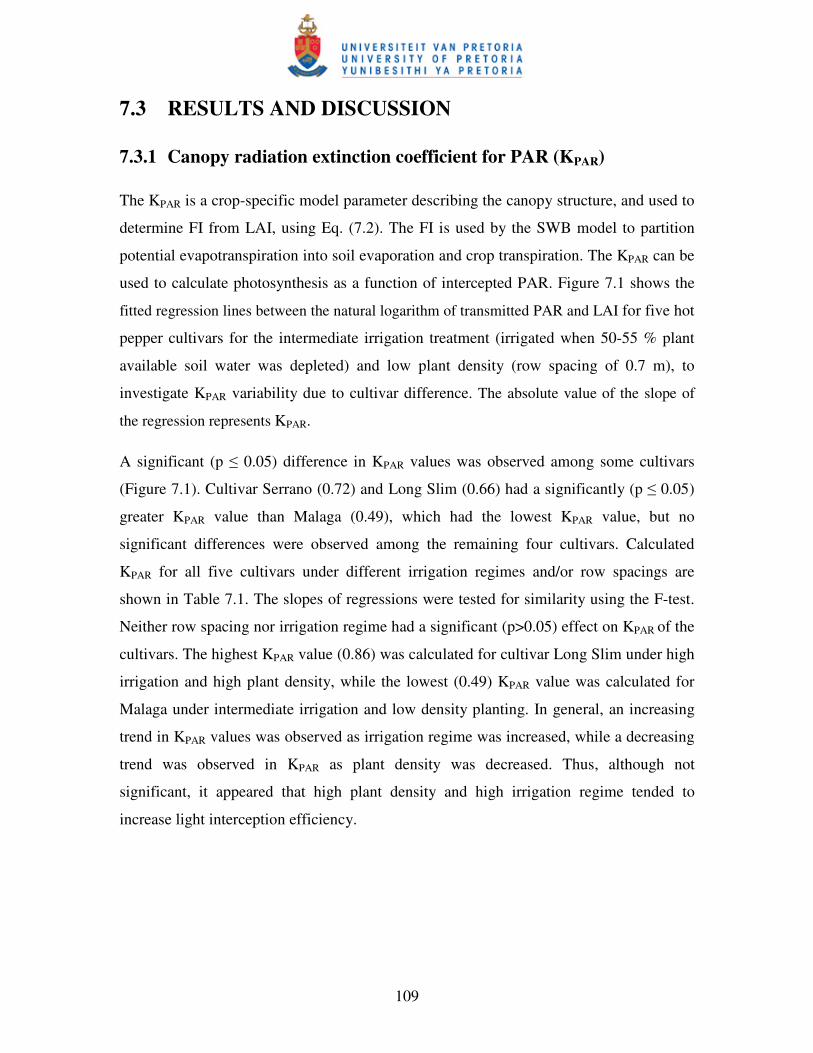
109


7.3.1 Canopy radiation extinction coefficient for PAR (KPAR)

The KPAR is a crop-specific model parameter describing the canopy structure, and used to

determine FI from LAI, using Eq. (7.2). The FI is used by the SWB model to partition

potential evapotranspiration into soil evaporation and crop transpiration. The KPAR can be

used to calculate photosynthesis as a function of intercepted PAR. Figure 7.1 shows the

fitted regression lines between the natural logarithm of transmitted PAR and LAI for five hot

pepper cultivars for the intermediate irrigation treatment (irrigated when 50-55 % plant

available soil water was depleted) and low plant density (row spacing of 0.7 m), to

investigate KPAR variability due to cultivar difference. The absolute value of the slope of

the regression represents KPAR.

A significant (p � 0.05) difference in KPAR values was observed among some cultivars

(Figure 7.1). Cultivar Serrano (0.72) and Long Slim (0.66) had a significantly (p � 0.05)

greater KPAR value than Malaga (0.49), which had the lowest KPAR value, but no

significant differences were observed among the remaining four cultivars. Calculated

KPAR for all five cultivars under different irrigation regimes and/or row spacings are

shown in Table 7.1. The slopes of regressions were tested for similarity using the F-test.

Neither row spacing nor irrigation regime had a significant (p>0.05) effect on KPAR of the

cultivars. The highest KPAR value (0.86) was calculated for cultivar Long Slim under high

irrigation and high plant density, while the lowest (0.49) KPAR value was calculated for

Malaga under intermediate irrigation and low density planting. In general, an increasing

trend in KPAR values was observed as irrigation regime was increased, while a decreasing

trend was observed in KPAR as plant density was decreased. Thus, although not

significant, it appeared that high plant density and high irrigation regime tended to

increase light interception efficiency.

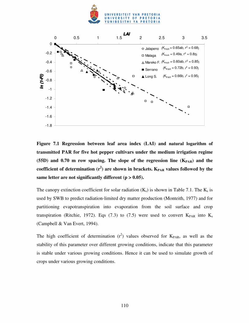
110

LAILAILAILAI

-1.8

-1.6

-1.4

-1.2

-1

-0.8

-0.6

-0.4

-0.2

0

0 0.5 1 1.5 2 2.5 3 3.5ln

(1-F

I)ln

(1-F

I)ln

(1-F

I)ln

(1-F

I)

Jalapeno

Malaga

Mareko F.

Serrano

Long S.

(KPAR = 0.65ab, r2 = 0.68)

(KPAR = 0.49a, r2 = 0.85)

(KPAR = 0.60ab, r2 = 0.85)

(KPAR = 0.72b, r2 = 0.93)

(KPAR = 0.66b, r2 = 0.95)

Figure 7.1 Regression between leaf area index (LAI) and natural logarithm of

transmitted PAR for five hot pepper cultivars under the medium irrigation regime

(55D) and 0.70 m row spacing. The slope of the regression line (KPAR) and the

coefficient of determination (r2) are shown in brackets. KPAR values followed by the

same letter are not significantly different (p > 0.05).

The canopy extinction coefficient for solar radiation (Ks) is shown in Table 7.1. The Ks is

used by SWB to predict radiation-limited dry matter production (Monteith, 1977) and for

partitioning evapotranspiration into evaporation from the soil surface and crop

transpiration (Ritchie, 1972). Eqs (7.3) to (7.5) were used to convert KPAR into Ks

(Campbell & Van Evert, 1994).

The high coefficient of determination (r2) values observed for KPAR, as well as the

stability of this parameter over different growing conditions, indicate that this parameter

is stable under various growing conditions. Hence it can be used to simulate growth of

crops under various growing conditions.

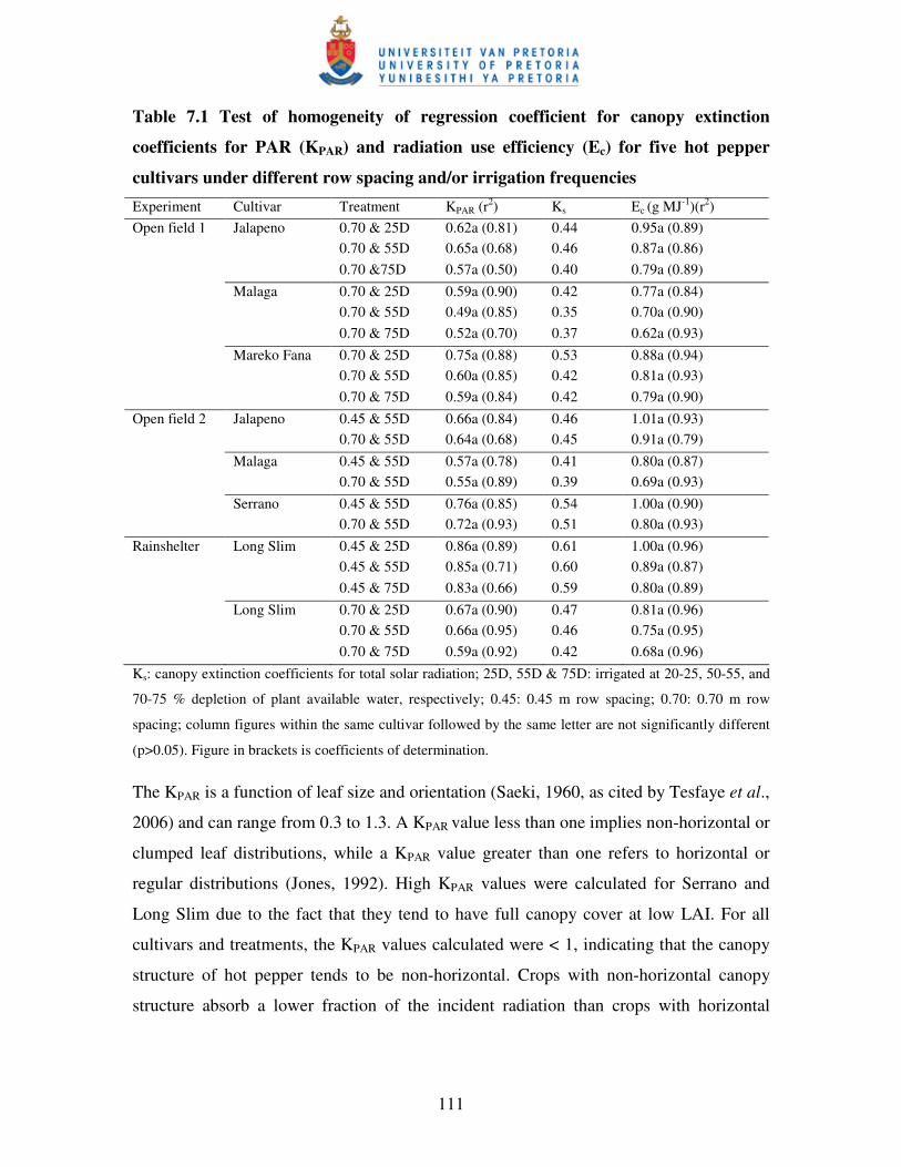
111

Table 7.1 Test of homogeneity of regression coefficient for canopy extinction

coefficients for PAR (KPAR) and radiation use efficiency (Ec) for five hot pepper

cultivars under different row spacing and/or irrigation frequencies Experiment Cultivar Treatment KPAR (r2) Ks Ec (g MJ-1)(r2) Open field 1 Jalapeno 0.70 & 25D 0.62a (0.81) 0.44 0.95a (0.89) 0.70 & 55D 0.65a (0.68) 0.46 0.87a (0.86) 0.70 &75D 0.57a (0.50) 0.40 0.79a (0.89) Malaga 0.70 & 25D 0.59a (0.90) 0.42 0.77a (0.84) 0.70 & 55D 0.49a (0.85) 0.35 0.70a (0.90) 0.70 & 75D 0.52a (0.70) 0.37 0.62a (0.93) Mareko Fana 0.70 & 25D 0.75a (0.88) 0.53 0.88a (0.94) 0.70 & 55D 0.60a (0.85) 0.42 0.81a (0.93) 0.70 & 75D 0.59a (0.84) 0.42 0.79a (0.90) Open field 2 Jalapeno 0.45 & 55D 0.66a (0.84) 0.46 1.01a (0.93) 0.70 & 55D 0.64a (0.68) 0.45 0.91a (0.79) Malaga 0.45 & 55D 0.57a (0.78) 0.41 0.80a (0.87) 0.70 & 55D 0.55a (0.89) 0.39 0.69a (0.93) Serrano 0.45 & 55D 0.76a (0.85) 0.54 1.00a (0.90) 0.70 & 55D 0.72a (0.93) 0.51 0.80a (0.93) Rainshelter Long Slim 0.45 & 25D 0.86a (0.89) 0.61 1.00a (0.96) 0.45 & 55D 0.85a (0.71) 0.60 0.89a (0.87) 0.45 & 75D 0.83a (0.66) 0.59 0.80a (0.89) Long Slim 0.70 & 25D 0.67a (0.90) 0.47 0.81a (0.96) 0.70 & 55D 0.66a (0.95) 0.46 0.75a (0.95) 0.70 & 75D 0.59a (0.92) 0.42 0.68a (0.96) Ks: canopy extinction coefficients for total solar radiation; 25D, 55D & 75D: irrigated at 20-25, 50-55, and

70-75 % depletion of plant available water, respectively; 0.45: 0.45 m row spacing; 0.70: 0.70 m row

spacing; column figures within the same cultivar followed by the same letter are not significantly different

(p>0.05). Figure in brackets is coefficients of determination.

The KPAR is a function of leaf size and orientation (Saeki, 1960, as cited by Tesfaye et al.,

2006) and can range from 0.3 to 1.3. A KPAR value less than one implies non-horizontal or

clumped leaf distributions, while a KPAR value greater than one refers to horizontal or

regular distributions (Jones, 1992). High KPAR values were calculated for Serrano and

Long Slim due to the fact that they tend to have full canopy cover at low LAI. For all

cultivars and treatments, the KPAR values calculated were < 1, indicating that the canopy

structure of hot pepper tends to be non-horizontal. Crops with non-horizontal canopy

structure absorb a lower fraction of the incident radiation than crops with horizontal

112

canopy structure at low LAI (Jovanovic et al., 1999), suggesting that hot pepper is

inefficient in radiation interception.

Canopy radiation extinction coefficient for PAR (KPAR) was reported to be affected by

difference in soil water (Tesfaye et al., 2006), row spacings (Flénet et al., 1996;

Jovanovic et al., 2002) and cultivar (Kiniry et al., 1989). Flénet et al. (1996) reported a

significant increment in KPAR of sunflower, soybean, sorghum and maize as row spacing

decreased from 1.00 to 0.35 m, indicating greater radiation interception efficiency in

narrow rows. According to Flénet et al. (1996), this improvement in radiation

interception ability of the crops was attributed to the result of a more even distribution of

the plants and hence of the foliage. The lack of significant differences in KPAR values in

the present study was probably due to the selection of two row spacings which were not

sufficiently different from each other. Furthermore, detecting the presence of significant

changes in KPAR due to a treatment effect may be confounded, as KPAR is a coefficient of

an empirical equation that models a complex phenomenon like canopy height, canopy

width and leaf orientation over the course of time (Flénet et al., 1996).

7.3.2 Radiation use efficiency (Ec)

The Ec is a crop-specific model parameter used to calculate dry matter production under

conditions of radiation-limited growth, using Eq. (7.6) (Monteith, 1977). Figure 7.2

presents DM of five hot pepper cultivars, under intermediate irrigation and low density

planting, as a function of the daily cumulative product of FI and PAR. The slope of the

regression line forced through the origin represents the efficiency of conversion of

intercepted radiation to dry matter.

Calculated Ec for all five cultivars under different irrigation regimes and/or row spacings

are shown in Table 7.1. The slopes of regressions were tested for similarity using the F-

test. Both high irrigation regime (25D) and high density plantings (0.45 m) tended to

increase Ec values, although their effects on Ec were not significant (P>0.05). The highest

Ec value was calculated for cultivar Jalapeno (1.01 g MJ-1) under medium irrigation

regime and narrow row spacing, while the lowest Ec value was calculated for cultivar

Malaga (0.62 g MJ-1) under low irrigation regime and wide row spacing (Table 7.2).

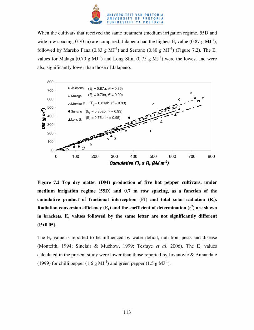
113

When the cultivars that received the same treatment (medium irrigation regime, 55D and

wide row spacing, 0.70 m) are compared, Jalapeno had the highest Ec value (0.87 g MJ-1),

followed by Mareko Fana (0.83 g MJ-1) and Serrano (0.80 g MJ-1) (Figure 7.2). The Ec

values for Malaga (0.70 g MJ-1) and Long Slim (0.75 g MJ-1) were the lowest and were

also significantly lower than those of Jalapeno.

0

100

200

300

400

500

600

700

800

0 100 200 300 400 500 600 700 800Cumulative FICumulative FICumulative FICumulative FIssss x R x R x R x Rssss (MJ m (MJ m (MJ m (MJ m-2-2-2-2))))

DM

(g m

DM

(g m

DM

(g m

DM

(g m

-2-2 -2-2)) ))

Jalapeno

Malaga

Mareko F.

Serrano

Long S.

(Ec = 0.87a, r2 = 0.86)

(Ec = 0.70b, r2 = 0.90)

(Ec = 0.81ab, r2 = 0.93)

(Ec = 0.80ab, r2 = 0.93)

(Ec = 0.75b, r2 = 0.95)

Figure 7.2 Top dry matter (DM) production of five hot pepper cultivars, under

medium irrigation regime (55D) and 0.7 m row spacing, as a function of the

cumulative product of fractional interception (FI) and total solar radiation (Rs).

Radiation conversion efficiency (Ec) and the coefficient of determination (r2) are shown

in brackets. Ec values followed by the same letter are not significantly different

(P>0.05).

The Ec value is reported to be influenced by water deficit, nutrition, pests and disease

(Monteith, 1994; Sinclair & Muchow, 1999; Tesfaye et al. 2006). The Ec values

calculated in the present study were lower than those reported by Jovanovic & Annandale

(1999) for chilli pepper (1.6 g MJ-1) and green pepper (1.5 g MJ-1).

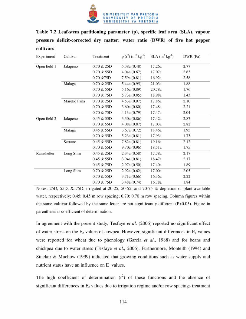
114

Table 7.2 Leaf-stem partitioning parameter (p), specific leaf area (SLA), vapour

pressure deficit-corrected dry matter: water ratio (DWR) of five hot pepper

cultivars Experiment Cultivar Treatment p (r2) (m2 kg-1) SLA (m2 kg-1) DWR (Pa)

Open field 1 Jalapeno 0.70 & 25D 5.38a (0.48) 17.26a 2.77 0.70 & 55D 4.04a (0.67) 17.07a 2.63 0.70 &75D 7.59a (0.81) 16.92a 2.58 Malaga 0.70 & 25D 5.44a (0.95) 21.03a 1.88 0.70 & 55D 5.16a (0.89) 20.78a 1.76 0.70 & 75D 5.73a (0.85) 18.98a 1.43 Mareko Fana 0.70 & 25D 4.53a (0.97) 17.86a 2.10 0.70 & 55D 3.60a (0.80) 17.48a 2.21 0.70 & 75D 4.13a (0.79) 17.47a 2.04 Open field 2 Jalapeno 0.45 & 55D 3.30a (0.86) 17.42a 2.87 0.70 & 55D 4.08a (0.87) 17.03a 2.82 Malaga 0.45 & 55D 3.67a (0.72) 18.46a 1.95 0.70 & 55D 5.23a (0.81) 17.93a 1.73 Serrano 0.45 & 55D 7.82a (0.81) 19.16a 2.12 0.70 & 55D 9.70a (0.96) 18.51a 1.75 Rainshelter Long Slim 0.45 & 25D 2.34a (0.58) 17.78a 2.17 0.45 & 55D 3.94a (0.81) 18.47a 2.17 0.45 & 75D 2.97a (0.50) 17.40a 1.89 Long Slim 0.70 & 25D 2.92a (0.62) 17.00a 2.05 0.70 & 55D 3.71a (0.66) 16.36a 2.22 0.70 & 75D 3.48a (0.74) 16.78a 1.84

Notes: 25D, 55D, & 75D: irrigated at 20-25, 50-55, and 70-75 % depletion of plant available

water, respectively; 0.45: 0.45 m row spacing; 0.70: 0.70 m row spacing. Column figures within

the same cultivar followed by the same letter are not significantly different (P>0.05). Figure in

parenthesis is coefficient of determination.

In agreement with the present study, Tesfaye et al. (2006) reported no significant effect

of water stress on the Ec values of cowpea. However, significant differences in Ec values

were reported for wheat due to phenology (Garcia et al., 1988) and for beans and

chickpea due to water stress (Tesfaye et al., 2006). Furthermore, Monteith (1994) and

Sinclair & Muchow (1999) indicated that growing conditions such as water supply and

nutrient status have an influence on Ec values.

The high coefficient of determination (r2) of these functions and the absence of

significant differences in Ec values due to irrigation regime and/or row spacings treatment

115

suggest that Ec is a relatively stable and predictable parameter in hot peppers. However,

Ec values need to be determined for individual cultivars, as a marked difference was

observed across cultivars, not only in this study but also between this study and that of

Jovanovic & Annandale (1999).

7.3.3 Specific leaf area and leaf-stem partitioning parameter

Table 7.2 presents the leaf-stem partitioning parameters for the five hot pepper cultivars

under different irrigation regimes and/or row spacings. Figure 7.3 shows the leaf-stem

partitioning parameters for the five hot pepper cultivars for the medium irrigation regime

(55D) and low plant density (0.70 m) treatments.

The SLA is used by SWB to calculate LAI using Eq. (7.9).The SLA was calculated as the

seasonal average of the ratio of LAI to LDM. Analysis of variance was conducted to test

whether treatments significantly affected SLA values of the hot pepper cultivars. SLA

values for the five cultivars under different irrigation regimes and/or row spacings are

shown in Table 7.2. Table 7.3 shows the SLA values for the five hot pepper cultivars

when exposed to the same treatments (medium irrigation regime and narrow row

spacing).

Significant differences in the leaf-stem partitioning parameter were observed among

cultivars (Figure 7.3). Cultivar Serrano had significantly higher leaf-stem partitioning

parameter (9. 70 m2 kg-1) than the other four cultivars. Neither irrigation regime nor row

spacing significantly affected leaf-stem partitioning parameters (Table 7.2). However,

although the effect was small and not significant, wide row sapcing appeared to increase

the leaf-stem partitioning parameter.

The leaf-stem partitioning parameter values calculated here were higher than those

reported by Jovanovic & Annandale (1999) for chilli pepper (1.04 m2 kg-1) and green

pepper (1.07 m2 kg-1). This is probably due to the low SLA and canopy dry matter values

recorded by Jovanovic & Annandale (1999). Due to the fact that leaf-stem partitioning

parameter is a coefficient of an empirical equation that models a complex phenomenon

like leaf mass, leaf area and stem mass over the course of time, it may be difficult to

detect marked differences emanating from changes in irrigation regime and/or row

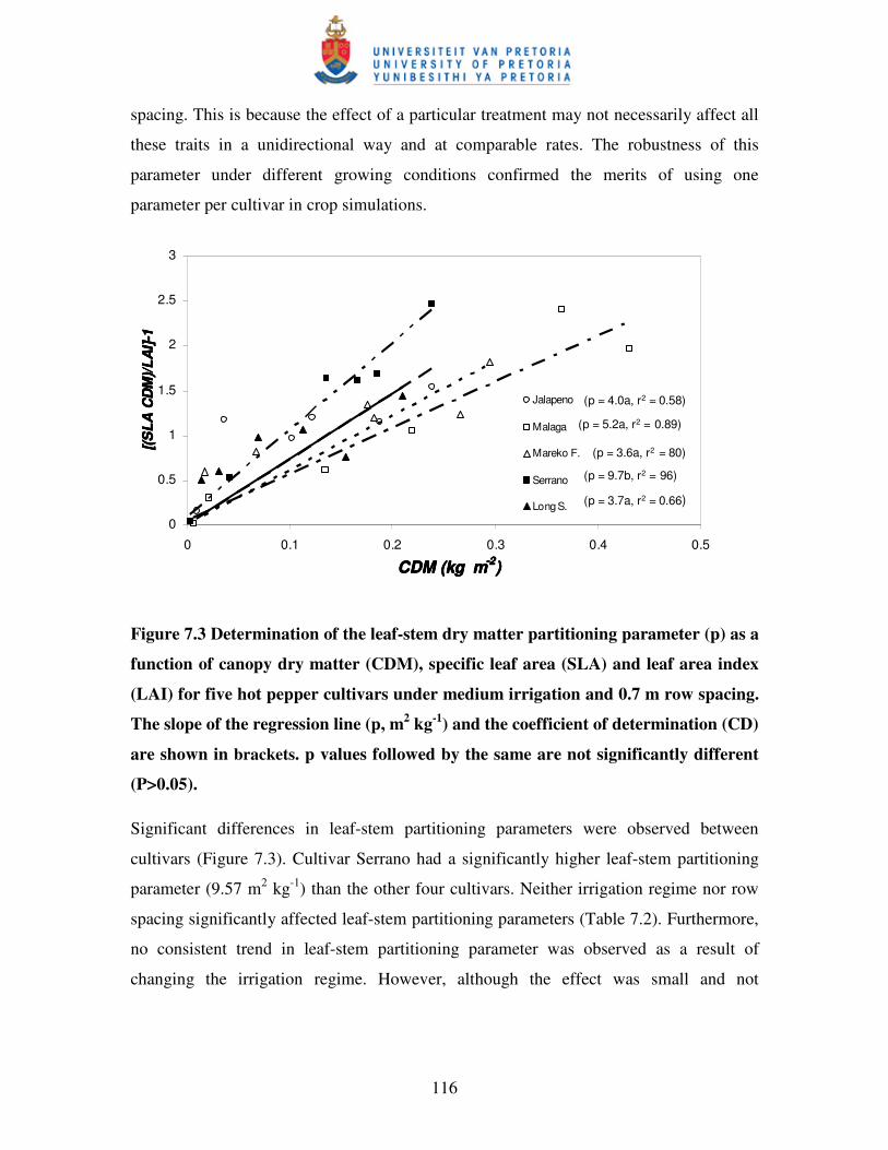
116

spacing. This is because the effect of a particular treatment may not necessarily affect all

these traits in a unidirectional way and at comparable rates. The robustness of this

parameter under different growing conditions confirmed the merits of using one

parameter per cultivar in crop simulations.

0

0.5

1

1.5

2

2.5

3

0 0.1 0.2 0.3 0.4 0.5

CDM (kg mCDM (kg mCDM (kg mCDM (kg m-2-2-2-2))))

[(SLA

CD

M)/L

AI]-

1[(S

LA C

DM

)/LA

I]-1

[(SLA

CD

M)/L

AI]-

1[(S

LA C

DM

)/LA

I]-1

Jalapeno

Malaga

Mareko F.

Serrano

Long S.

(p = 4.0a, r2 = 0.58)

(p = 5.2a, r2 = 0.89)

(p = 3.6a, r2 = 80)

(p = 9.7b, r2 = 96)

(p = 3.7a, r2 = 0.66)

Figure 7.3 Determination of the leaf-stem dry matter partitioning parameter (p) as a

function of canopy dry matter (CDM), specific leaf area (SLA) and leaf area index

(LAI) for five hot pepper cultivars under medium irrigation and 0.7 m row spacing.

The slope of the regression line (p, m2 kg-1) and the coefficient of determination (CD)

are shown in brackets. p values followed by the same are not significantly different

(P>0.05).

Significant differences in leaf-stem partitioning parameters were observed between

cultivars (Figure 7.3). Cultivar Serrano had a significantly higher leaf-stem partitioning

parameter (9.57 m2 kg-1) than the other four cultivars. Neither irrigation regime nor row

spacing significantly affected leaf-stem partitioning parameters (Table 7.2). Furthermore,

no consistent trend in leaf-stem partitioning parameter was observed as a result of

changing the irrigation regime. However, although the effect was small and not

117

significant, low density planting appeared to increase the leaf-stem partitioning

parameter.

Neither irrigation regime nor row spacings significantly affected specific leaf area (SLA)

(Table 7.2). Variable SLA values were observed among the cultivars (Table 7.3). Cultivar

Malaga (20.78 m2 kg-1) had the higher SLA followed by Serrano (18.51 m2 kg-1), Mareko

Fana (17.48 m2 kg-1), Jalapeno (17.07 m2 kg-1), and Long Slim (16.36 m2 kg-1).

SLA is shown to be a stable crop-specific parameter under different irrigation regimes

and/or row spacings. Hence, the robustness of these parameters under different growing

conditions confirmed the merits of using one parameter per cultivar in crop simulations.

Cultivar difference in these parameters deserves important consideration as significant

differences was observed due to cultivar.

Table 7.3 Specific leaf area (SLA), vapour pressure-corrected dry matter: water

ratio (DWR), day degrees to 50% flowering (DDF) and maturity (DDM) for five hot

pepper cultivars under 0.7 m row spacing and medium irrigation regime (55D) Cultivar SLA (m2 kg-1) VPD (Pa) DWR (Pa) DDF (d °C) DDM (d °C)

Jalapeno 17.07 1045 2.77 450 1290

Malaga 20.78 1035 1.76 690 1530

Mareko Fana 17.48 1024 2.21 470 1330

Serrano 18.51 1045 1.75 470 1425

Long Slim 16.36 1046 2.22 570 1295

7.3.4 Vapour pressure deficit-corrected dry matter/water ratio (DWR)

Transpiration efficiency is influenced by climate, notably vapour pressure deficit (VPD)

(Tanner & Sinclair, 1983). DWR is a crop-specific parameter measuring water use

(transpiration) efficiency by accounting for variation in atmospheric conditions,

especially for VPD. Table 7.2 shows DWR as affected by different irrigation regimes

and/or row spacings. DWR values for the five hot pepper cultivars exposed to the same

treatments (intermediate irrigation and low plant density) are shown in Table 7.3.

Statistical analysis for DWR was not done as data are obtained for single observations. Of

118

the cultivars, Jalapeno had the highest DWR value, followed by Mareko Fana, Long

Slim, Serrano and Malaga. Generally, high irrigation regime and decreased row spacing

increased the DWR.

DWR values reported for hot pepper in the present study (1.73 – 2.87 Pa) are lower than

those reported by Jovanovic et al. (1999) for chilli (4.5 Pa) and green peppers (4.5 Pa).

The probable reason for the marked difference in DWR values between the two studies is

the high potential transpiration and the low Ec calculated in the present study, as

compared to that of Jovanovic et al. (1999). This, in turn, is due to high FI and growing

day degrees to maturity recorded in the present study, compared to Jovanovic et al.

(1999). The results of the present study indicated the presence of a positive association

between radiation conversion efficiency (Ec) and DWR, while DWR seemed to relate

negatively with growing day degrees to maturity.

7.3.5 Thermal time requirements

Growing day degrees (GDD) for the five hot pepper cultivars to 50% flowering and

maturity were determined and are presented in Table 7.3. Marked differences in GDD for

both 50% flowering and maturity were observed. Cultivar Jalapeno attained both 50%

flowering (450 d °C) and maturity (1290 d °C) earlier than the other cultivars, while

Malaga reached 50% flowering (690 d °C) and maturity (1530 d °C) later than the other

cultivars.

7.3.6 Crop-specific model parameters for newly released cultivars

The ability to predict crop-specific model parameters that would likely fit new hot pepper

cultivars is imperative, as new cultivars are released regularly due to market demand and

the broad genetic basis of the species. Furthermore, the time and resources required for

determining crop-specific model parameters for new cultivars is usually prohibitive.

Important features of the five cultivars considered in this study are shown in Table 7.4.

Figure 6.3 shows photos of hot pepper cultivars used in the experiments. Accordingly, a

new cultivar with near horizontal canopy structure, similar to Long Slim and Serrano will

probably have KPAR values between 0.60 and 0.80. On the other hand, for a cultivar with

119

vertically oriented leaves, like Jalapeno, it seems appropriate to assign a KPAR value

around 0.45. In between these categories, cultivars whose canopy structure ranges

between vertically oriented leaves and near horizontal leaf arrangements, similar to

Malaga and Mareko Fana, may have KPAR values in the range of 0.45 to 0.65.

Similarly, a new early maturing cultivar with a small canopy and medium dry matter

production capacity (like Jalapeno), or with medium maturity, large canopy and with high

dry matter production (like Mareko Fana) can have an Ec value >0.9 g MJ-1. For new

cultivars with early maturity, medium canopy size and low dry matter production (like

Long Slim), or with late maturity, large canopy and medium to high dry matter

production (like Malaga) it appears appropriate to assign an Ec value of around 0.70 to

0.80 g MJ-1. A cultivar with medium maturity, medium canopy and with low dry matter

production (like Serrano) will probably have an Ec value around 0.8 g MJ-1. For Serrano

and Long Slim cultivars there is a need to increase the Ec value at least by 0.2 g MJ-1 as

row width is decreased from 0.7 m to 0.45 m.

The leaf-stem partitioning parameter for all cultivars, except Serrano ranged between

2.34 and 7.59 m2 kg-1, and therefore new cultivars that do not share Serrano’s features,

will probably have their leaf-stem partitioning parameters in the range of 2.34 and 7.59

m2 kg-1. A cultivar with high stem mass in relation to leaf and with medium canopy size

(similar to Serrano) should be assigned a leaf-stem partitioning parameter value of around

8.5 m2 kg-1.

A cultivar with early maturity, small canopy and medium dry matter production (like

Jalapeno) can have a DWR value around 2.5 Pa and above. A cultivar with medium

maturity, large canopy and with high dry matter production (like Mareko Fana), or with

short maturity, medium canopy and with low dry matter production (like Long Slim) can

have a DWR value between 1.9 and 2.2 Pa. A cultivar with long maturity, large canopy

and with high dry matter production capacity (like Malaga), or with medium maturity,

medium canopy and with low dry matter production (like Serrano) should have a DWR

value of around 1.8 Pa. Increasing the DWR from the reported values is necessary, as the

DWR reported here represents the lower limit since underground dry matter is not

120

included in the determination of DWR and furthermore, potential transpiration instead of

actual transpiration was utilized in calculation.

Generally, understanding features of hot pepper cultivars for which crop-specific model

parameters were determined can aid to estimate parameters that likely best fit new

cultivars. Cultivar features such as time to maturity, canopy structure and size, and level

of dry matter production are important when trying to adapt crop-specific parameters of a

cultivar to new cultivars whose cultivar-specific model parameters are not yet

experimentally determined.

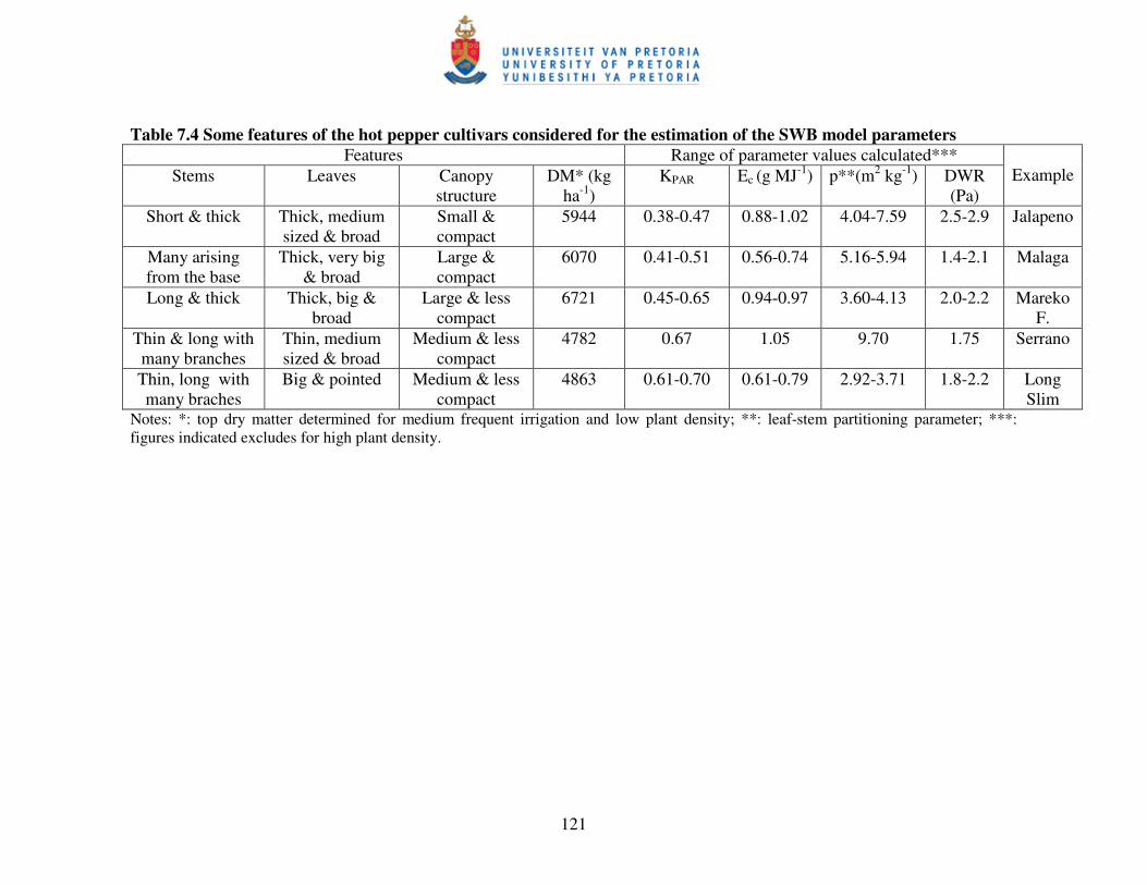
121

Table 7.4 Some features of the hot pepper cultivars considered for the estimation of the SWB model parameters

Features Range of parameter values calculated*** Stems Leaves Canopy

structure DM* (kg

ha-1) KPAR Ec (g MJ-1) p**(m2 kg-1) DWR

(Pa)

Example

Short & thick Thick, medium sized & broad

Small & compact

5944 0.38-0.47 0.88-1.02 4.04-7.59 2.5-2.9 Jalapeno

Many arising from the base

Thick, very big & broad

Large & compact

6070 0.41-0.51 0.56-0.74 5.16-5.94 1.4-2.1 Malaga

Long & thick Thick, big & broad

Large & less compact

6721 0.45-0.65 0.94-0.97 3.60-4.13 2.0-2.2 Mareko F.

Thin & long with many branches

Thin, medium sized & broad

Medium & less compact

4782 0.67 1.05 9.70 1.75 Serrano

Thin, long with many braches

Big & pointed Medium & less compact

4863 0.61-0.70 0.61-0.79 2.92-3.71 1.8-2.2 Long Slim

Notes: *: top dry matter determined for medium frequent irrigation and low plant density; **: leaf-stem partitioning parameter; ***: figures indicated excludes for high plant density.

122

7.4 CONCLUSIONS

Results of the study showed that almost all crop-specific model parameters studied

appeared to remain stable under different irrigation regimes and row spacings. This is

attributed to the fact that most of these crop-specific model parameters integrate more

than two variables over the course of time, and therefore treatments might not affect them

in similar ways and rates across all variables. However, a significant difference in almost

all of the crop-specific model parameters was observed due to cultivar differences. This

reflects inherent cultivar variability in their ability to capture resources (solar radiation,

water) and convert these resources into dry matter. Therefore, it was concluded that the

investigated crop-specific model parameters should be transferable to simulate growth

and irrigation scheduling over different irrigation regimes and row spacing. However,

caution must be exercised against adopting crop-specific model parameters developed for

a particular cultivar for other cultivars whose crop-specific model parameters have not

yet been determined.

Understanding cultivar features like time to maturity, canopy structure and size, and level

of dry matter production are important when trying to adapt crop-specific model

parameters of a cultivar to new cultivars whose cultivar-specific model parameters have

not yet been experimentally determined.

123

CHAPTER 8

THERMAL TIME REQUIREMENTS FOR THE

DEVELOPMENT OF HOT PEPPER (Capsicum annuum L.)

Abstract

Pant development is sensitive to temperature and understanding temperature response

function helps to model growth using cardinal temperatures. The objective of this

investigation was to quantify temperature response functions of various developmental

stages of two hot pepper cultivars (Jalapeno and Mareko Fana). Cardinal temperatures,

namely the base (Tb), optimum (Tm) and cut-off temperature (Tx) for various

developmental stages were also determined. Jalapeno and Mareko Fana were investigated

in four growth cabinets; each at constant temperature, ranging from 10 to 32.5 °C, in

steps of 7.5 °C. Results from the growth cabinet study were evaluated using independent

field data collected from field experiments. A Tb of 8.5 °C, Tm of 24 °C and Tx of 36 °C

describe germination of the cultivar Jalapeno. A Tb of 13.5 °C, Tm of 22 °C and Tx of 40

°C describe post-germination developmental stages of Jalapeno. A Tb of 12.5 °C, Tm of

21.5 °C and Tx of 35 °C describe post-germination developmental stages of Mareko Fana.

Thermal time requirements from transplanting to flowering ranged from 198 °C d to 280

°C d and from transplanting to maturity ranged from 799 °C d to 913 °C d for the two

cultivars in the growth cabinet and open field studies.

Keywords: cardinal temperatures, germination, hot pepper, germination, thermal time

124

8.1 INTRODUCTION

Temperature, solar radiation, water and nutrients are the most important abiotic variables

that affect plant growth and development and the quantification of their effects on plants

form the basis of simulation models of crop production (Atkinson & Porter, 1996).

However, distinction needs to be made between the effects of these variables on growth

and development as these two processes involve different aspects of plant processes.

According to Atkinson & Porter (1996), growth is defined as an irreversible increase in

dry matter, resulting from the maintenance of disequilibrium between the accumulation

and the loss of environmental resources. On the other hand, developmental processes are

recognized either via changes in number of plant organs, or via the time taken for

particular morphological events, such as flowering to occur.

Growth is more affected by total radiation received, rather than temperature (Monteith,

1977), whereas plant development is sensitive to temperature (Monteith, 1981; Hodges,

1991). Temperature increment or decrement even for a few degrees usually leads to a

remarkable change in developmental changes in plants. The effect of temperature on

plant development rate is often described by using the thermal time, or ‘heat unit’

concept. Particularly in the area of crop phenology and development, the concept of heat

units, measured in growing-degree-days (GDD, °C-day), has vastly improved description

and prediction of phenological events compared to other approaches such as time of the

year or number of days (Russelle, et al. 1984; McMaster & Smika, 1988; McMaster &

Wilhelm. 1997). Consequently, the thermal time concept is getting wider application in

crop modelling. One widely used thermal time quantification approach is the one which

relates developmental rate (DR) linearly to temperature above a crop or cultivar specific

base temperature, at or below which the developmental rate remains zero (Tollenaar et

al., 1979), plus in some applications with addition of maximum temperature above which

DR remains constant (Hodges, 1991). Gilmore & Rogers (1958) as cited by Yin et al.

(1995) presented a bilinear model that included a reversal linear function to account for

the declining DR at temperatures higher than optimum temperature when describing the

elongation of maize seedlings in relation to temperature. Yin et al. (1995) used a beta

function to describe the relationship between temperatures and DR. In spite of the

125

variation in the mathematical models used to describe the relationship between DR and

temperature, most models recognize three sets of temperatures which are: base

temperature, maximum temperature and optimum temperature in describing the DR-

temperature models. At base and maximum temperatures growth is assumed to stop,

whereas at optimum temperature developmental rate proceeds at its maximum rate. These

temperatures are known as cardinal temperatures and are important in the calculation of

thermal time (GDD) (Campbell & Norman, 1998).

The fact that from germination to fruit setting and maturity, plants require different

temperature regimes necessitates quantification of the response of the hot pepper

developmental stages to different temperatures. Furthermore, the wide genotypic

variations within the hot pepper species (Bosland, 1992) make it important to determine

the cardinal temperatures for a particular cultivar. Knowledge about hot pepper response

to different regimes of temperature for different growth stages and identification of the

cardinal temperatures would help to improve modelling this crop’s development. Thus,

growth cabinet and field experiments were conducted with the following objectives:

1. to determine cardinal temperatures for various developmental stages germination,

emergence, vegetative, flowering, and fruit maturity) of hot pepper,

2. to quantify the thermal time requirements for these developmental stages, and

3. to validate the growth chamber results with an independent data set from field

experiments.

126


Growth cabinets and field trials were carried out in this study. In the growth cabinet

studies, the cardinal temperatures for germination and subsequent developmental stages

were estimated, which were then used to calculate thermal time requirements. A

comparison was then made between thermal time requirements determined in the growth

cabinets at constant temperature and those observed in the field trials under fluctuating

temperatures.

8.2.1 Germination study

The study was conducted at the Hatfield Experimental Farm of the University of Pretoria,

Pretoria, under controlled conditions from April 7 to May 15, 2006. Hot pepper cultivar

Jalapeno was used in the study. Seeds were germinated in Petri dishes lined with filter

paper at four different constant temperatures, ranging from 10 to 32.5 °C in a growth

cabinet; in steps of 7.5 °C. The filter paper was first soaked in distilled water and then

100 seeds were spread on the filter paper. Treatments were replicated three times. Daily

inspection was made to note germination progress. Water was applied daily. Germination

was defined as the protrusion of the radicle through the testa by more than 5 mm. The

average results of the cultivar from the three replicates were plotted against time to obtain

a germination progression curve. From these curves, the time taken to reach certain

cumulative germination percentages could be determined through interpolation.

8.2.2 Developmental stage experiments

The study was conducted at the Hatfield Experimental Farm the University of Pretoria,

Pretoria, under controlled conditions from 5 October 2005 to 10 May 2006. Four growth

cabinets and two cultivars (Mareko Fana and Jalapeno) were used to quantify response in

rates of development to temperature changes. The former cultivar is a cultivar that grows

widely in Ethiopia and the latter one is from South Africa. Both cultivars were grown in

four cabinets, each at constant temperature, ranging from 10 to 32.5 °C, in steps of 7.5 °C.

Later, Mareko Fana was grown at 29 °C in a separate growth cabinet due to the failure of

127

the crop to flower at 32.5 °C. Photoperiod was maintained at 13 hrs (quantitative short

day plant) for all treatments (Demers & Gosselin, 2002).

Six-week-old hot pepper seedlings of the respective cultivars were transplanted into a

growth medium consisting of a fine river sand and vermiculite mixture (1:1 v/v), in 3 litre

pots. Twenty pots per cultivar were placed in each growth cabinet. Two seedlings were

planted per pot and later thinned to one plant after the seedlings survived the

transplanting shock. Pots were watered daily with a complete nutrient solution and excess

nutrient solution was allowed to drain freely through openings at the bottom of the pots.

Shuffling of the pots in a cabinet was done weekly to limit the effect of uneven air and

light distribution within the cabinets.

For the emergence study, 50 seeds of each cultivar were sown in seedling trays at the

temperatures specified above. Daily inspection was made to note emergence progress.

Water was applied daily. Emergence was defined as the protrusion of the plumule

(cotyledon) through the soil surface by more than 5 mm. The average results of the

cultivar from the two replicates were plotted against time to obtain an emergence

progression curve. A specific growth stage was reached when 50% of the seeds in

seedling trays or plants in growth cabinets achieved the developmental stage being

considered (emergence, leaf number, flowering or maturity).

8.2.3 Field experiment

An independent data set from a field study conducted at the University of Pretoria,

Hatfield Experimental Farm during the 2004/05 growing season was used to validate results

of the growth chamber studies.

8.2.4 Data collection and analysis

8.2.4.1 Cardinal temperature determination

Cardinal temperatures for germination, emergence, vegetative stage, flowering, and

maturity were determined by fitting linear functions to temperature and developmental

rate data. Base temperature and maximum temperatures were taken as the lower and

128

higher temperature values when the development rate becomes zero. The temperature

where development rate reached a maximum was assumed to be the optimal. The rate of

development was calculated as the reciprocal of the time needed for the completion of a

particular developmental stage concerned.

8.2.4.2 Thermal time determination

Using cardinal temperatures as input, the thermal time (�) for different temperatures was

determined both for plants grown under growth cabinet and field conditions, using the

following equations (Monteith, 1977; Campbell & Norman, 1998, Olivier & Annandale,

1998):

xb TTT >>= 0τ (8.1)

( ) mbb TTTtTT <<∆−=τ (8.2)

( )( )( ) xm

mx

bmx TTTtTT

TTTT<<∆�

�

�

�

−−−

=τ (8.3)

Where T is the average of the daily maximum and minimum temperatures when the

increment �t is taken as 1 day, Tb is base temperature, Tm is the optimum temperature

and Tx the maximum temperature. Below Tb and above Tx, no thermal time will be

accumulated and it is assumed that no development takes place (Eq. (8.1)). According to

Eq. (8.2), thermal time increases linearly between Tb and Tm. Between Tm and Tx thermal

time decreases linearly (Eq. (8.3)).

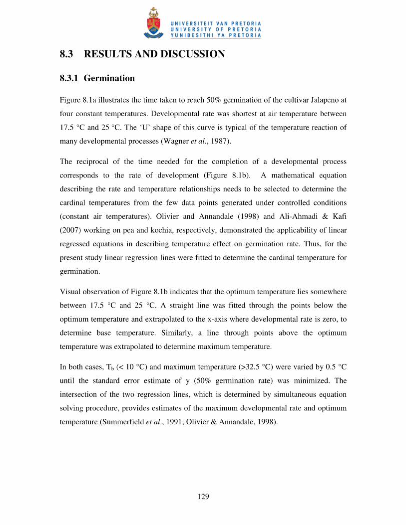
129


8.3.1 Germination

Figure 8.1a illustrates the time taken to reach 50% germination of the cultivar Jalapeno at

four constant temperatures. Developmental rate was shortest at air temperature between

17.5 °C and 25 °C. The ‘U’ shape of this curve is typical of the temperature reaction of

many developmental processes (Wagner et al., 1987).

The reciprocal of the time needed for the completion of a developmental process

corresponds to the rate of development (Figure 8.1b). A mathematical equation

describing the rate and temperature relationships needs to be selected to determine the

cardinal temperatures from the few data points generated under controlled conditions

(constant air temperatures). Olivier and Annandale (1998) and Ali-Ahmadi & Kafi

(2007) working on pea and kochia, respectively, demonstrated the applicability of linear

regressed equations in describing temperature effect on germination rate. Thus, for the

present study linear regression lines were fitted to determine the cardinal temperature for

germination.

Visual observation of Figure 8.1b indicates that the optimum temperature lies somewhere

between 17.5 °C and 25 °C. A straight line was fitted through the points below the

optimum temperature and extrapolated to the x-axis where developmental rate is zero, to

determine base temperature. Similarly, a line through points above the optimum

temperature was extrapolated to determine maximum temperature.

In both cases, Tb (< 10 °C) and maximum temperature (>32.5 °C) were varied by 0.5 °C

until the standard error estimate of y (50% germination rate) was minimized. The

intersection of the two regression lines, which is determined by simultaneous equation

solving procedure, provides estimates of the maximum developmental rate and optimum

temperature (Summerfield et al., 1991; Olivier & Annandale, 1998).

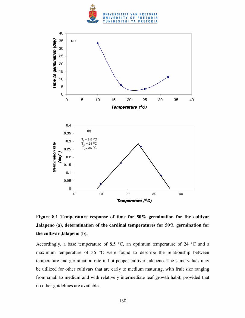
130

(a)

0

5

10

15

20

25

30

35

40

0 5 10 15 20 25 30 35 40

Temperature (Temperature (Temperature (Temperature (ooooC)C)C)C)

Tim

e to

ger

min

atio

n (d

ay)

Tim

e to

ger

min

atio

n (d

ay)

Tim

e to

ger

min

atio

n (d

ay)

Tim

e to

ger

min

atio

n (d

ay)

(b)

Tb = 8.5 OCTm = 24 OCTx = 36 OC

0

0.05

0.1

0.15

0.2

0.25

0.3

0.35

0.4

0 10 20 30 40

Temperature (Temperature (Temperature (Temperature (OOOOC)C)C)C)

Ge

rmin

ati

on

ra

te

Ge

rmin

ati

on

ra

te

Ge

rmin

ati

on

ra

te

Ge

rmin

ati

on

ra

te

(da

y(d

ay

(da

y(d

ay-1-1 -1-1

)) ))

Figure 8.1 Temperature response of time for 50% germination for the cultivar

Jalapeno (a), determination of the cardinal temperatures for 50% germination for

the cultivar Jalapeno (b).

Accordingly, a base temperature of 8.5 °C, an optimum temperature of 24 °C and a

maximum temperature of 36 °C were found to describe the relationship between

temperature and germination rate in hot pepper cultivar Jalapeno. The same values may

be utilized for other cultivars that are early to medium maturing, with fruit size ranging

from small to medium and with relatively intermediate leaf growth habit, provided that

no other guidelines are available.

131

Thermal time requirements for 50% germination of Jalapeno seed, at constant

temperatures, were calculated using the estimated cardinal temperatures and Eqs. (8.1)-

(8.3). Results for the cultivar Jalapeno are presented in Figure 8.2. The thermal time

requirements for 50% germination for Jalapeno varied between 51 and 62 day degrees

when calculated for four different constant air temperatures using cardinal temperatures

determined in the study.

The small variation in thermal time expressed by the low coefficient of variation (CV

=2.4%) and standard error estimate (SE = 1.9 °C d) revealed that a linear thermal time

expression can be used to model seed germination of hot pepper cultivar Jalapeno. An

average day degree value of 56 appeared reasonably acceptable to use as thermal time

requirements for 50% germination for the cultivar Jalapeno and other cultivars that are

early to medium maturing, with fruit size ranging from small to medium and with

relatively intermediate leaf growth habit in the absence of other research results.

SE = 1.9 SE = 1.9 SE = 1.9 SE = 1.9 OOOOC dC dC dC dCV = 2.4 %CV = 2.4 %CV = 2.4 %CV = 2.4 %

5154 56

62

0

10

20

30

40

50

60

70

10 17.5 25 32.5

Temperature (Temperature (Temperature (Temperature (0000C)C)C)C)

The

rmal

tim

e (

The

rmal

tim

e (

The

rmal

tim

e (

The

rmal

tim

e (OO OO

C d

)C

d)

C d

)C

d)

Figure 8.2 Thermal time requirement for 50% germination, calculated at four

constant temperatures for the cultivar Jalapeno.

132

8.3.2 Developmental stages

Figures 8.3a and 8.3b show the time required from sowing to reach various

developmental stages for the cultivars Jalapeno and Mareko Fana, respectively. Different

authors used different mathematical expressions to quantify temperature effect on rates of

different developmental stages. Various mathematical expressions are used depending on

the variability of species, temperature regimes or process being simulated. Omanga et al.

(1995) and Olivier & Annandale (1998) used bilinear equations to describe the response

of pigeon pea and pea crop developmental rate to temperature, respectively, while Yin et

al. (1995) using cassava, maize and rice, suggested asymmetric functions (the Beta

function) to describe developmental rate and temperature relationship. Wagner et al.

(1987) employed exponential functions to describe relationships between developmental

rate of insects and temperature. In the present study, owing to the limited data points (3

pairs of data points in most cases) two linear regression lines were fitted to determine the

cardinal temperatures for developmental stages (Figures 8.4a and 8.4b).

In order to simplify the description and prediction of phenological events and modelling

of hot pepper, an effort was made to determine a single set of cardinal temperatures

describing the different developmental stages. Visual observation does not give much

clue as to the optimum temperature range due to the limited data points (Figures 8.3a and

8.3b). However, from the relationship between temperature and rates of germination

(Figure 8.1a) and emergence (8.3a), it could be assumed, with a reasonable degree of

accuracy, that the optimum temperature falls between 17.5 and 25 °C. Furthermore, the

extremely low rate of flowering observed at the extreme high temperatures suggests that

optimum temperature for the same process falls between 17.5 and 25 °C and not between

25 and 29°C (in Mareko Fana) or 25 and 32.5 °C (in Jalapeno). Thus, two temperatures,

i.e., 25 and 32.5 °C in Jalapeno and 25 and 29 °C in Mareko Fana were used to estimate

maximum temperature.

Developmental rate is zero at a maximum temperature, so by arbitrarily selecting a

maximum temperature above 32.5 °C for Jalapeno and 29 °C for Mareko Fana, three

points were available for the linear regression lines between 25 °C and maximum

temperature. The standard error of the y estimates of the regression lines for the

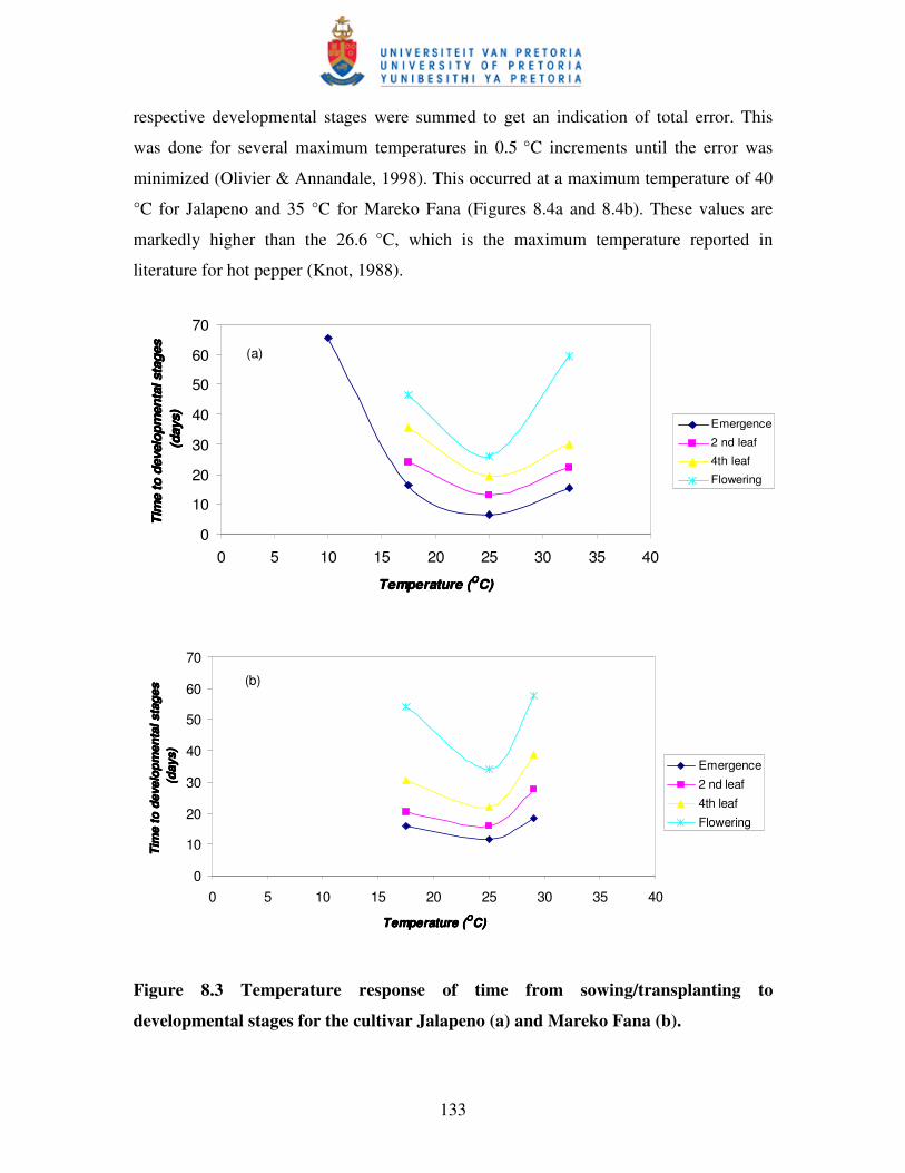
133

respective developmental stages were summed to get an indication of total error. This

was done for several maximum temperatures in 0.5 °C increments until the error was

minimized (Olivier & Annandale, 1998). This occurred at a maximum temperature of 40

°C for Jalapeno and 35 °C for Mareko Fana (Figures 8.4a and 8.4b). These values are

markedly higher than the 26.6 °C, which is the maximum temperature reported in

literature for hot pepper (Knot, 1988).

(a)

0

10

20

30

40

50

60

70

0 5 10 15 20 25 30 35 40


Tim

e to

dev

elop

men

tal s

tage

s Ti

me

to d

evel

opm

enta

l sta

ges

Tim

e to

dev

elop

men

tal s

tage

s Ti

me

to d

evel

opm

enta

l sta

ges

(day

s)(d

ays)

(day

s)(d

ays) Emergence

2 nd leaf

4th leaf

Flowering

(b)

0

10

20

30

40

50

60

70

0 5 10 15 20 25 30 35 40


Tim

e to

dev

elop

men

tal s

tage

s Ti

me

to d

evel

opm

enta

l sta

ges

Tim

e to

dev

elop

men

tal s

tage

s Ti

me

to d

evel

opm

enta

l sta

ges

(day

s)(d

ays)

(day

s)(d

ays)

Emergence2 nd leaf4th leafFlowering

Figure 8.3 Temperature response of time from sowing/transplanting to

developmental stages for the cultivar Jalapeno (a) and Mareko Fana (b).

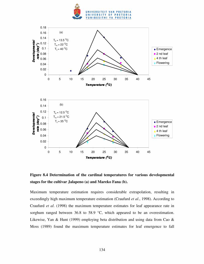
134

(a)

Tb = 13.5 OC

Tm = 22 OC

Tx = 40 OC

0

0.02

0.04

0.06

0.08

0.1

0.12

0.14

0.16

0.18

0 5 10 15 20 25 30 35 40 45


De

velo

pm

en

tal

De

velo

pm

en

tal

De

velo

pm

en

tal

De

velo

pm

en

tal

rate

(d

ay

rate

(d

ay

rate

(d

ay

rate

(d

ay-1-1 -1-1

)) ))

Emergence2 nd leaf4 th leafFlowering

(b)

Tb = 12.5 OC

Tm = 21.5 OC

Tx = 35 OC

0

0.02

0.04

0.06

0.08

0.1

0.12

0.14

0.16

0 5 10 15 20 25 30 35 40 45


De

velo

pm

en

tal

De

velo

pm

en

tal

De

velo

pm

en

tal

De

velo

pm

en

tal

rate

(d

ay

rate

(d

ay

rate

(d

ay

rate

(d

ay-1-1 -1-1

)) ))

Emergence2 nd leaf4 th leafFlowering

Figure 8.4 Determination of the cardinal temperatures for various developmental

stages for the cultivar Jalapeno (a) and Mareko Fana (b).

Maximum temperature estimation requires considerable extrapolation, resulting in

exceedingly high maximum temperature estimation (Craufurd et al., 1998). According to

Craufurd et al. (1998) the maximum temperature estimates for leaf appearance rate in

sorghum ranged between 36.8 to 58.9 °C, which appeared to be an overestimation.

Likewise, Yan & Hunt (1999) employing beta distribution and using data from Cao &

Moss (1989) found the maximum temperature estimates for leaf emergence to fall

135

between 43.3 and 50 °C for wheat genotypes, and between 42.5 and 46.4 °C for barley

genotypes.

Temperatures between 17.5 and 25 °C were randomly selected in 0.5 °C increments to

estimate optimum temperatures of the respective cultivars with the assumption that the

optimum temperature falls between 17.5 and 25 °C. Four points are therefore available,

including the maximum temperature for estimating the optimum temperature. Linear

regression lines were fitted using four points for all developmental stages considered. The

standard error of the y estimates of the regression lines for the respective developmental

stages were summed to get an indication of total error. Optimum temperature was

assumed at the temperature (x value) where the total standard error of the y estimate of

the regressions of all developmental stages was at a minimum. Error was minimized at

Tm of 22 °C for Jalapeno and 21.5 °C for Mareko Fana (Figures 8.4a and 8.4b). Knot

(1988) reported an optimum temperature of 22.5 °C for hot pepper, which appears to

agree with the present results for the cultivar Jalapeno, whereas optimum temperature for

Mareko Fana seems markedly lower than the value reported in literature.

The same procedure described above was utilized to determine base temperature. Here

three data points (including the optimum temperature) are available. The total standard

error of the y estimates for developmental stages was at the minimum at a base

temperature of 13 °C for Jalapeno and 12.5 °C for Mareko Fana (Figures 8.4a and 8.4b).

Knot (1988) reported a base temperature of 11 °C, which appears to be sufficiently lower

than the present results, suggesting the need to consider genotypic differences.

Hot peppers require day temperatures of 24-30 °C and night temperatures of 10-15 °C for

optimum growth (Smith et al., 1998). The present study confirmed the fact that too high a

night temperature is more detrimental to reproductive development than the vegetative

growth as either flowering failed to materialize at 32.5 °C in Mareko Fana or it occurred

after roughly 3 months at 29 °C in Mareko Fana and at 32.5 °C in Jalapeno. Thus, if

emphasis is given to modelling of flowering and fruit maturity it is reasonable to use

maximum temperature values lower that the values reported here as these traits were

hardly expressed at high constant day and night temperatures. On the contrary, if

136

emphasis is given to emergence and vegetative growth, it appears that considering high

values for maximum temperature are reasonable.

8.3.3 Validating results with field data

The cardinal temperatures determined in the growth cabinets for each cultivar were used

to calculate thermal time requirements for flowering and maturity stages in the field

(Figure 8.5). The thermal time requirement in both cultivars was determined from the

growth cabinet average constant temperature of 25 °C for flowering and maturity

(harvest) using separate cardinal temperatures for individual cultivars. The reason for

using the above constant temperature is that this is the only constant temperature where

both cultivars achieved flowering and maturity.

In the field, Mareko Fana required 280 °C d for flowering and 913 °C d for maturity,

while Jalapeno required 242 °C d for flowering and 799 °C d for maturity. In the growth

cabinet, Mareko Fana required 227 °C d for flowering and 860 °C d for maturity, while

Jalapeno required 198 °C d for flowering and 816 °C d for maturity. Mareko Fana

seedlings in the growth cabinets flowered four days earlier than those in the open fields,

while Jalapeno seedlings in the growth cabinets flowered five days earlier than those in

the open fields. The prediction error for maturity was five days for Mareko Fana and nine

days for Jalapeno. This is probably due to the fact that seedlings in the open field

experienced severe transplanting shock and, therefore, took longer to acclimatize in the

new environment, which is much harsher in the open field environment. Olivier &

Annandale (1998) cited the spatial and temporal temperature variations between growth

cabinet and field conditions for the observed difference in thermal time requirements for

various developmental stages of peas grown in growth cabinets and open field.

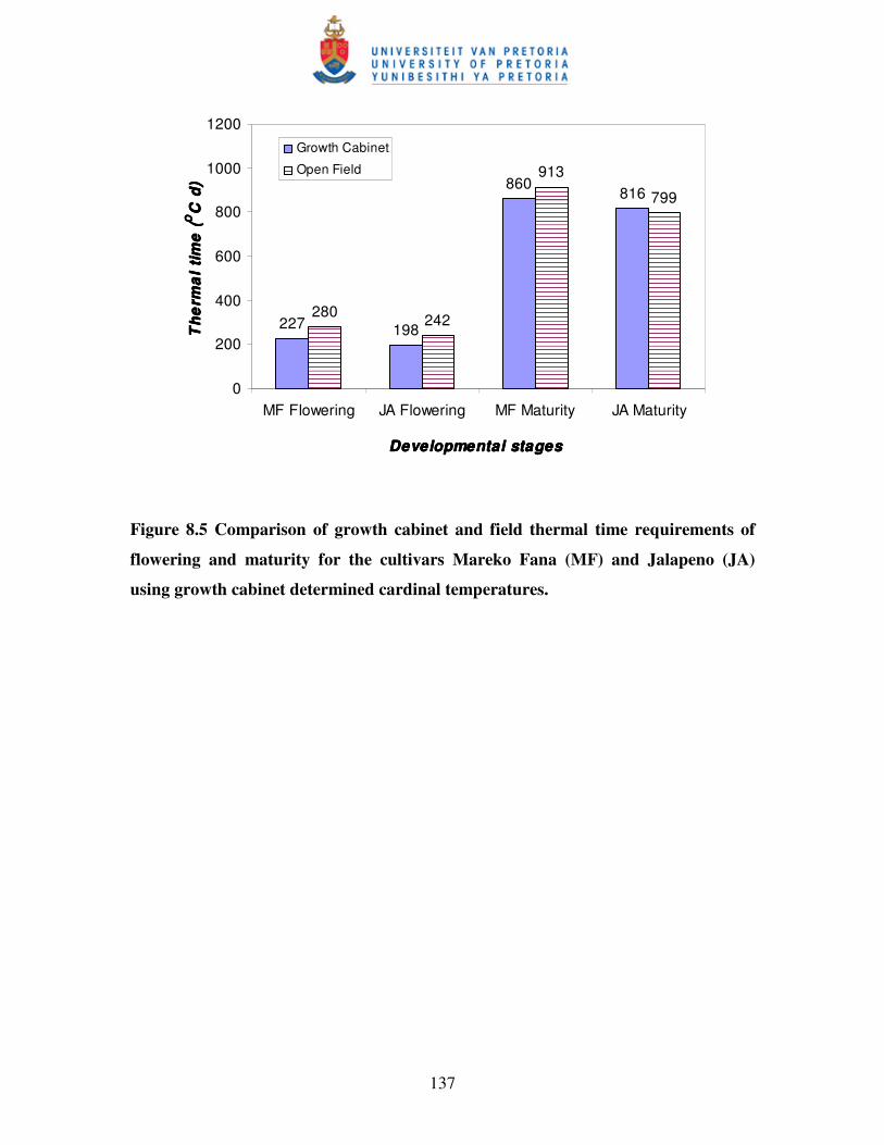
137

227 198

860816

280 242

913

799

0

200

400

600

800

1000

1200

MF Flowering JA Flowering MF Maturity JA Maturity

Developmental stagesDevelopmental stagesDevelopmental stagesDevelopmental stages

Th

erm

al

tim

e (

Th

erm

al

tim

e (

Th

erm

al

tim

e (

Th

erm

al

tim

e (

OO OOC

d)

C d

)C

d)

C d

)

Growth Cabinet

Open Field

Figure 8.5 Comparison of growth cabinet and field thermal time requirements of

flowering and maturity for the cultivars Mareko Fana (MF) and Jalapeno (JA)

using growth cabinet determined cardinal temperatures.

138

8.4 CONCLUSIONS

It appears that a marked difference exists between hot pepper cultivars with respect to

their cardinal temperatures, especially maximum temperatures and thus thermal time

requirements to complete different developmental stages. Distinction needs to be made

between vegetative and flowering stages, as these developmental stages behave

differently to low and high temperatures, in that high temperatures significantly limit the

development rate of reproductive growth while the effect on vegetative rate is minimal.

For sake of simplicity, a base temperature of 12.5 °C and optimum temperature of 22 °C

seems to be reasonably acceptable for the hot pepper cultivars studied here. However,

retaining the maximum temperature values of individual cultivars is recommended, as the

results for the two cultivars appeared to differ markedly.

Knowledge of the cardinal temperatures and the thermal time requirements for the

developmental stages of hot pepper can enhance nursery management and planning of

operations like transplanting and harvesting. It also improves scheduling of staggered

planting and prediction of harvest time from the use of long-term average temperature for

continuous supply of fresh produce to the market. Furthermore, understanding the

cardinal temperatures and thermal time requirements of individual cultivars would

improve the modelling of respective hot pepper cultivars for simulating growth and

irrigation scheduling.

139

CHAPTER 9

CALIBRATION AND VALIDATION OF THE SWB

IRRIGATION SCHEDULING MODEL FOR HOT PEPPER

(Capsicum annuum L.) CULTIVARS FOR CONTRASTING

PLANT POPULATIONS AND IRRIGATION REGIMES

Abstract

Irrigation is standard practice in hot pepper production and sound irrigation scheduling

increases productivity. Irrigation can be scheduled using various tools, including

computer modelling. The Soil Water Balance (SWB) model is a mechanistic, generic

crop irrigation scheduling model. Calibration and validation of the model using reliable

data is required to ensure accurate simulations. Detailed weather, soil and crop data were

collected from three field trials conducted in the 2004/05 growing season at the Hatfield

Experimental Farm, University of Pretoria. Model calibration was done using crop-

specific model parameters determined under optimum growing conditions, while model

validation was done using data generated under water stress and/or low planting density

conditions. The SWB model was successfully calibrated for the cultivars Jalapeno, Long

Slim and Serrano for most growth parameters and the soil water deficit was predicted

with reasonable accuracy. Validation simulations were inside or marginally outside the

reliability criteria imposed for deficit irrigation treatments. However, caution must be

exercised when using crop-specific model parameters developed under optimum plant

population to simulate growth under low plant population conditions, as most of the

validation simulations were outside the reliability criteria for Long Slim under low

density planting and deficit irrigation treatments. This is due to the fact that the SWB

model does not account for plant population.

Keywords: hot pepper, irrigation regime, irrigation scheduling, plant population, SWB

model

140

9.1 INTRODUCTION

Hot pepper (Capsicum annuum L.) is a warm season, high value cash crop. Generally, its

production is confined to areas where available water is limited and, therefore, irrigation

is standard practice in hot pepper production (Wein, 1998). The crop is sensitive to water

stress (Delfine et al., 2000). Both under- and over-irrigation is detrimental to the

profitability of crops. Under-irrigation may result in yield and quality reduction, while

over-irrigation could lead to excessive percolation, which has environmental

consequences and wastes water, nutrients and energy (to pump water).

Cultural practices such as variety (Ismail & Davies, 1997; Jaimez et al., 1999) and

planting density (Cantliffe & Phatak, 1975; O’Sullivan, 1980; Taylor et al., 1982; Tan et

al., 1983) were reported to influence plant response to irrigation water application.

Vigorously growing crops (cultivars) tend to exhaust soil water more rapidly than those

cultivars with a slower growth habit. Consequently, vigorous cultivars are usually

planted in wider rows to avoid competition among neighbouring plants and also to

prevent mutual shading of plant canopies (Jolliffe, 1988). Tan et al. (1983) reported

similar cucumber yield for high and low plant populations when grown without

irrigation, but they observed significant plant population effects under irrigated

conditions. Taylor (1980), working on soybean, observed no difference in yield among

0.25, 0.5, 0.75 and 1 m wide row spacings in 1976, a drier than normal growing season.

In the 1975 growing season with relatively normal rainfall, yield tended to increase as

row spacing decreased, but the differences were not significant. During 1977 with greater

than normal and preplant irrigation, soybeans in 0.25 m rows out-yielded those in 1.0 m

rows by 17%.

Models that incorporate such varied growing conditions would enhance our

understanding of how to manage agricultural inputs such as water and planting density

for profitable crop production and environmental protection. A large number of crop

physiological models have been developed for different applications (Sinclair &

Seligman, 1996). The Soil Water Balance (SWB) model is a mechanistic, user-friendly,

daily time step, generic crop growth and irrigation scheduling model (Annandale et al.,

141

1999). It is capable of simulating yield, different growth processes, and field water

balance components. This type of information can assist producers and researchers to

make decisions to alter inputs, maximize profit, and reduce soil erosion (Kiniry et al.,

1997).

Crop-specific model parameters can vary for different cultivars (Kiniry et al., 1989;

Annandale et al., 1999), vapour pressure deficit differences (Stockle & Kiniry, 1990),

irrigation frequencies (Tesfaye, 2006), row spacings (Flénet et al., 1996; Jovanovic et al.,

2002) and other growing conditions (Monteith, 1994; Sinclair & Muchow, 1999).

Furthermore, since crop models are often tested against long-term mean yields, models

for aiding decision making must be able to accurately simulate growth and yield in

extreme conditions (Xie et al., 2001).

Although crop-specific model parameters vary for different plant populations and

irrigation regimes, the SWB model has not been validated for various plant populations

and irrigation regimes in hot pepper. Therefore, this study was conducted to calibrate and

validate the SWB model for different hot pepper cultivars under contrasting plant

populations and/or irrigation regimes.

142



Details of the site and treatments are provided in paragraph 6.2.1 of Chapter 6.



the field. Drip irrigation was used in all three trials. Plants were irrigated for 1 hour (12.5-

15.5 mm) every other day for three weeks (until plants were well established). Thereafter,

plants were irrigated to field capacity, each time the treatments soil water deficit was

reached (Table 6.2). In the open field experiment 2 (where row spacings and cultivars are

the treatment), plants were irrigated to field capacity when 50-55% of plant available soil

water was depleted. Based on soil analysis results and target yield, 150 kg ha-1 N and 50

kg ha-1 K were applied to the rainshelter and to the open field experiments, the open field

experiment also received 75 kg ha-1 P. N application was split, with 50 kg ha-1 at planting,

followed by a 100 kg ha-1 top dressing eight weeks after transplant. Weeds were

controlled manually. Fungal diseases were controlled using Benomyl® (1H –

benzimidazole) and Bravo® (chlorothalonil) sprays, while red spider mites were

controlled with Metasystox® (oxydemeton–methyl) applied at the recommended doses.

Plots were regularly monitored and the number of plants attaining the flowering and

maturity stages was recorded. Dates of flowering and maturity were recorded when 50%

of the plants in a plot reached these stages.

Soil water deficit measurements were made using a model 503DR CPN Hydroprobe

neutron water meter (Campbell Pacific Nuclear, California, USA). Readings were taken

twice a week, at 0.2 m increments to a depth of 1.0 m, from access tubes installed in the

middle of each plot and positioned between rows.

Growth analyses were carried out at 15 to 25 day intervals by harvesting four plants from

a plot. Eight plants from the central two rows were reserved for yield measurements.

Fruits were harvested three times during the season. The sampled plants were separated

143

into leaves, stems and fruits, and oven dried to a constant mass. Leaf area was measured

with an LI 3100 belt driven leaf area meter (Li-Cor, Lincoln, Nebraska, USA).

The fraction of photosynthetically active radiation (PAR) intercepted by the canopy

(FIPAR) was measured using a sunfleck ceptometer (Decagon Devices, Pullman,

Washington, USA). The PAR measurements for a plot consisted of three series of

measurements conducted in rapid succession on cloudless days. A series of

measurements consisted of one reference reading above and ten readings beneath the

canopy, which were averaged. FIPAR was then calculated as follows:

��

��

�−=


FIPAR 1 9.1








9.2.3 The Soil Water Balance model

The Soil Water Balance (SWB) model is a mechanistic, real-time, user-friendly, generic

crop irrigation scheduling model (Annandale et al., 1999). It is based on the improved

version of the SWB model described by Campbell & Diaz (1988). The SWB model

contains three units, namely, weather, soil and crop unit. The weather unit of the SWB

model calculates the Penman-Monteith grass reference daily evapotranspiration (ETo)

according to the recommendations of the Food and Agriculture Organization of the

United Nations (Allen et al., 1998). The soil unit simulates the dynamics of soil water

movement (runoff, interception, infiltration, percolation, transpiration, soil water storage

and evaporation) in order to predict the soil water content. In the crop unit, the SWB

model calculates crop dry matter accumulation in direct proportion to transpiration

corrected for vapour pressure deficit (Tanner & Sinclair, 1983). The crop unit also

144

calculates radiation-limited growth (Monteith, 1977) and takes the lower value of the

two. This dry matter is partitioned into roots, stems, leaves and grains or fruits.

Partitioning depends on phenology, calculated with thermal time and modified by water

stress. The model also accounts for the effect of water stress on growth, reducing canopy

size by stress index parameter, the ratio between actual and potential transpiration. The

SWB model, however, does not have a routine to account for variations in plant

population.

The main strength of the SWB model compared to models that are more detailed is that it

requires fewer crop input parameters, while still predicting the crop growth and soil water

balance reasonably well. The generic nature of the SWB model further allows simulating

growth and soil water balance of several crops with the same user-friendly software

package, unlike species specific models (Jovanovic et al., 2000).

9.2.4 Determination of crop-specific model parameters

Field data collected from well-watered and/or high planting density treatments of three

field experiments during the 2004/05 growing season were used to estimate the following

crop-specific model parameters: radiation extinction coefficient, vapour pressure deficit-

corrected dry matter water ratio, radiation use efficiency, maximum crop height, day

degrees at the end of vegetative growth, day degrees for maturity, specific leaf area, and

leaf-stem partitioning parameters, following the procedures described by Jovanovic et al.

(1999). Furthermore, the crop-specific model parameters that were not generated from

field experiments were obtained from literature or estimated by calibrating the model

against measured field data.

9.2.5 Cultivars used in calibration and validation studies

Calibration and validation of the model was done for cultivars Jalapeno, Serrano and

Long Slim. Jalapeno is an early maturing cultivar with relatively large sized fruits and is

characterized by intermediate canopy growth. Serrano is an intermediate maturing

cultivar and bears small fruits and is characterized by relatively intermediate to prolific

145

canopy growth. Long Slim is an early maturing cultivar with medium sized fruits and

with an intermediate to prolific canopy growth.

9.2.6 Model reliability test

The SWB model calculates the following statistical parameters for testing model

prediction accuracy: Willmott’s (1982) index of agreement (d), the root mean square

error (RMSE), mean absolute error (MAE) and coefficient of determination (r2).

According to De Jager (1994), d and r2 values > 0.8 and MAE values < 0.2 indicate

reliable model predictions. RMSE reflects the magnitude of the mean difference between

predicted and measured values.

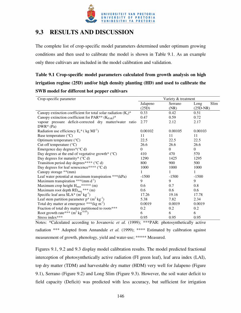
146


The complete list of crop-specific model parameters determined under optimum growing

conditions and then used to calibrate the model is shown in Table 9.1. As an example

only three cultivars are included in the model calibration and validation.

Table 9.1 Crop-specific model parameters calculated from growth analysis on high

irrigation regime (25D) and/or high density planting (HD) and used to calibrate the

SWB model for different hot pepper cultivars Variety & treatment Crop-specific parameter

Jalapeno (25D)

Serrano (NR)

Long Slim (25D-NR)

Canopy extinction coefficient for total solar radiation (Ks)* 0.33 0.42 0.51 Canopy extinction coefficient for PAR** (KPAR)* 0.47 0.59 0.72 vapour pressure deficit-corrected dry matter/water ratio DWR* (Pa)

2.77 2.12 2.17

Radiation use efficiency Ec* ( kg MJ-1) 0.00102 0.00105 0.00103 Base temperature (°C) 11 11 11 Optimum temperature (°C) 22.5 22.5 22.5 Cut-off temperature (°C) 26.6 26.6 26.6 Emergence day degrees*(°C d) 0 0 0 Day degrees at the end of vegetative growth* (°C) 410 470 570 Day degrees for maturity* (°C d) 1290 1425 1295 Transition period day degrees**** (°C d) 800 900 500 Day degrees for leaf senescence**** (°C d) 1000 1000 1000 Canopy storage **(mm) 1 1 1 Leaf water potential at maximum transpiration ***(kPa) -1500 -1500 -1500 Maximum transpiration ***(mm d-1) 9 9 9 Maximum crop height Hmax***** (m) 0.6 0.7 0.8 Maximum root depth RDmax *** (m) 0.6 0.6 0.6 Specific leaf area SLA* (m2 kg-1) 17.26 19.16 17.78 Leaf stem partition parameter p* (m2 kg-1) 5.38 7.82 2.34 Total dry matter at emergence ***(kg m-2) 0.0019 0.0019 0.0019 Fraction of total dry matter partitioned to roots*** 0.2 0.2 0.2 Root growth rate*** (m2 kg-0.05) 6 6 6 Stress index*** 0.95 0.95 0.95

Notes: *Calculated according to Jovanovic et al. (1999); ***PAR: photosynthetically active

radiation *** Adopted from Annandale et al. (1999); **** Estimated by calibration against

measurement of growth, phenology, yield and water-use; ***** Measured.

Figures 9.1, 9.2 and 9.3 display model calibration results. The model predicted fractional

interception of photosynthetically active radiation (FI green leaf), leaf area index (LAI),

top dry matter (TDM) and harvestable dry matter (HDM) very well for Jalapeno (Figure

9.1), Serrano (Figure 9.2) and Long Slim (Figure 9.3). However, the soil water deficit to

field capacity (Deficit) was predicted with less accuracy, but sufficient for irrigation

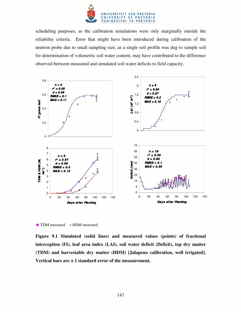
147

scheduling purposes, as the calibration simulations were only marginally outside the

reliability criteria. Error that might have been introduced during calibration of the

neutron probe due to small sampling size, as a single soil profile was dug to sample soil

for determination of volumetric soil water content, may have contributed to the difference

observed between measured and simulated soil water deficits to field capacity.

n = 6n = 6n = 6n = 6rrrr2222 = 0.90 = 0.90 = 0.90 = 0.90d = 0.96d = 0.96d = 0.96d = 0.96


0

0.2

0.4

0.6

0.8

FI

gre

en

le

af

FI

gre

en

le

af

FI

gre

en

le

af

FI

gre

en

le

af

n = 6n = 6n = 6n = 6rrrr2222 = 0.97 = 0.97 = 0.97 = 0.97d = 0.99d = 0.99d = 0.99d = 0.99


0

1

2

3

4

5

6

7

8

0 20 40 60 80 100 120 140

Days af ter PlantingDays af ter PlantingDays af ter PlantingDays af ter Planting

TD

M &

HD

M (

Mg

T

DM

& H

DM

(M

g

TD

M &

HD

M (

Mg

T

DM

& H

DM

(M

g

haha haha-1-1 -1-1

)) ))

n = 6n = 6n = 6n = 6rrrr2222 = 0.94 = 0.94 = 0.94 = 0.94d = 0.97d = 0.97d = 0.97d = 0.97


0

0.4

0.8

1.2

1.6

2

2.4

LA

I (m

LA

I (m

LA

I (m

LA

I (m

22 22 m m m m

-2-2 -2-2)) ))

n = 18n = 18n = 18n = 18 r r r r2222 = 0.56 = 0.56 = 0.56 = 0.56d = 0.80d = 0.80d = 0.80d = 0.80


-5

5

15

25

35

45

55

65

75

0 20 40 60 80 100 120 140


De

ficit

(mm

)D

efic

it (m

m)

De

ficit

(mm

)D

efic

it (m

m)

� TDM measured + HDM measured


interception (FI), leaf area index (LAI), soil water deficit (Deficit), top dry matter

(TDM) and harvestable dry matter (HDM) [Jalapeno calibration, well irrigated].

Vertical bars are ± 1 standard error of the measurement.

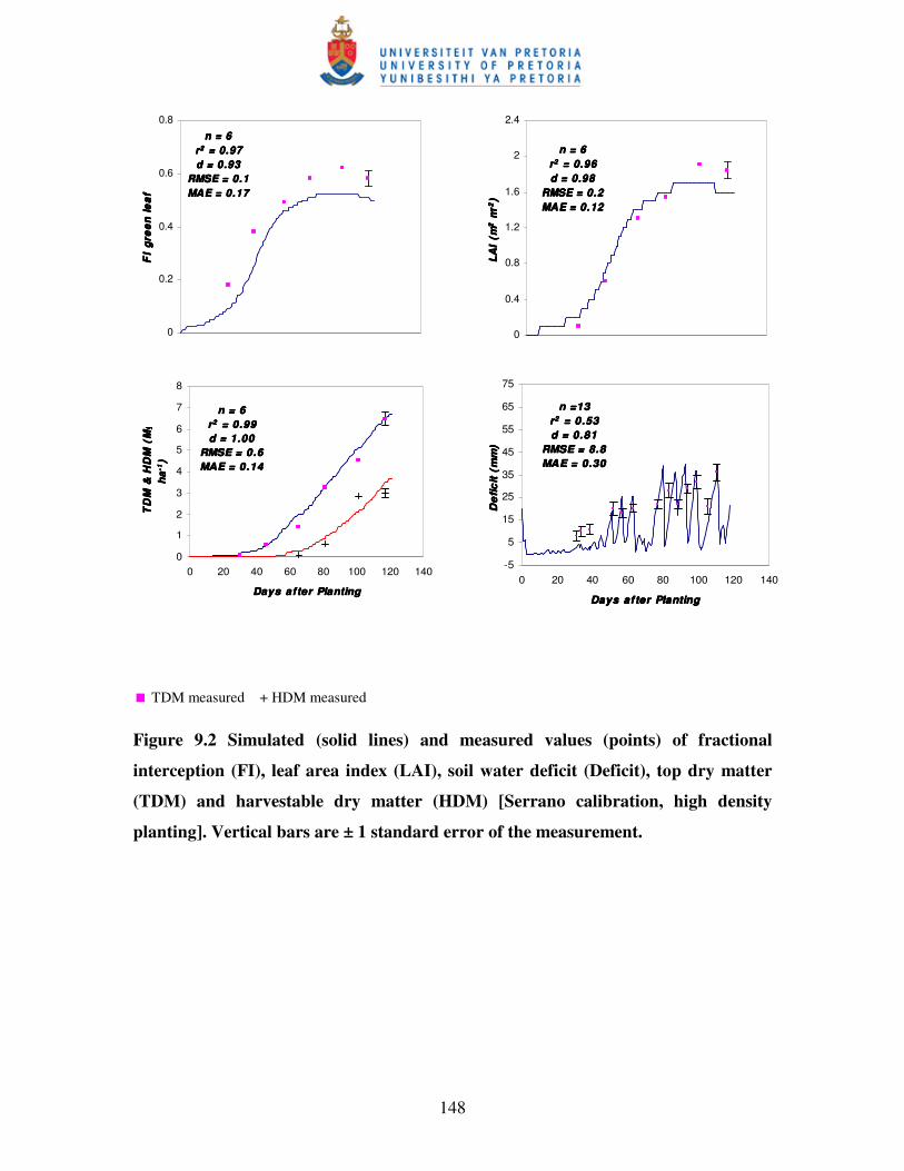
148

n = 6n = 6n = 6n = 6rrrr2222 = 0.97 = 0.97 = 0.97 = 0.97d = 0.93d = 0.93d = 0.93d = 0.93


0

0.2

0.4

0.6

0.8

FI

gre

en le

afF

I gr

een

leaf

FI

gre

en le

afF

I gr

een

leaf

n = 6n = 6n = 6n = 6rrrr2222 = 0.99 = 0.99 = 0.99 = 0.99d = 1.00d = 1.00d = 1.00d = 1.00


0

1

2

3

4

5

6

7

8

0 20 40 60 80 100 120 140

Days after PlantingDays after PlantingDays after PlantingDays after Planting

TD

M &

HD

M (

Mg

T

DM

& H

DM

(M

g

TD

M &

HD

M (

Mg

T

DM

& H

DM

(M

g

ha

ha

haha

-1-1 -1-1)) ))

n = 6n = 6n = 6n = 6rrrr2222 = 0.96 = 0.96 = 0.96 = 0.96d = 0.98d = 0.98d = 0.98d = 0.98


0

0.4

0.8

1.2

1.6

2

2.4

LAI

(mLA

I (m

LAI

(mLA

I (m

22 22 m m m m

-2-2 -2-2)) ))

n =13n =13n =13n =13rrrr2222 = 0.53 = 0.53 = 0.53 = 0.53d = 0.81d = 0.81d = 0.81d = 0.81


-5

5

15

25

35

45

55

65

75

0 20 40 60 80 100 120 140


De

ficit

(mm

)D

efic

it (m

m)

De

ficit

(mm

)D

efic

it (m

m)




(TDM) and harvestable dry matter (HDM) [Serrano calibration, high density

planting]. Vertical bars are ± 1 standard error of the measurement.

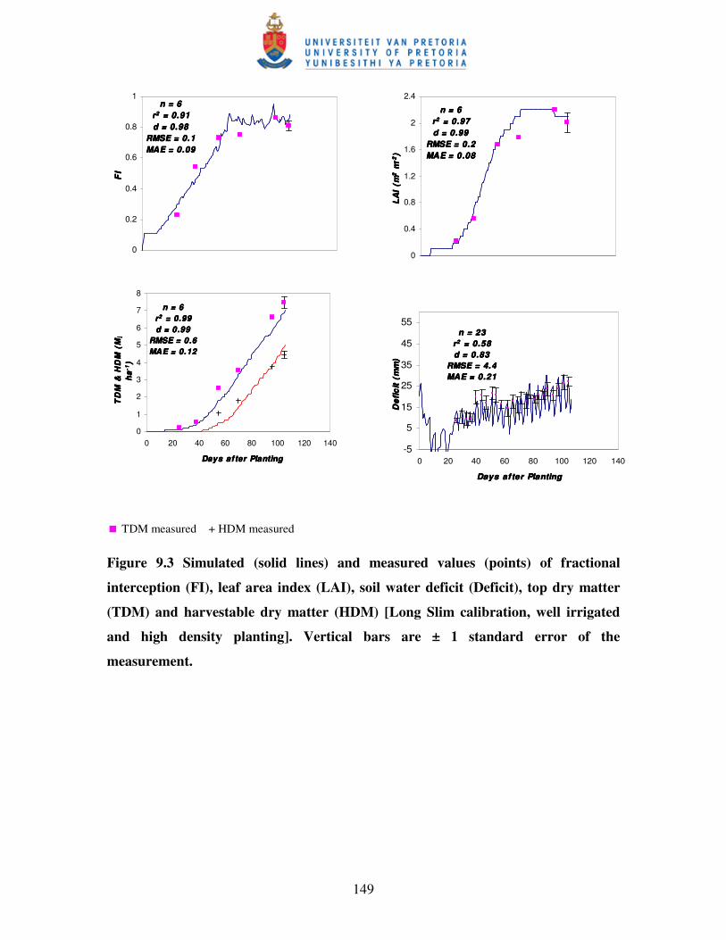
149

n = 6n = 6n = 6n = 6rrrr2222 = 0.91 = 0.91 = 0.91 = 0.91d = 0.98d = 0.98d = 0.98d = 0.98


0

0.2

0.4

0.6

0.8

1

FI

FI

FI

FI

n = 6n = 6n = 6n = 6rrrr2222 = 0.99 = 0.99 = 0.99 = 0.99d = 0.99d = 0.99d = 0.99d = 0.99


0

1

2

3

4

5

6

7

8

0 20 40 60 80 100 120 140


TD

M &

HD

M (

Mg

T

DM

& H

DM

(M

g

TD

M &

HD

M (

Mg

T

DM

& H

DM

(M

g

ha

ha

haha

-1-1 -1-1)) ))

n = 6n = 6n = 6n = 6rrrr2222 = 0.97 = 0.97 = 0.97 = 0.97d = 0.99d = 0.99d = 0.99d = 0.99


0

0.4

0.8

1.2

1.6

2

2.4

LA

I (m

LA

I (m

LA

I (m

LA

I (m

22 22 m m m m

-2-2 -2-2)) ))

n = 23n = 23n = 23n = 23rrrr2222 = 0.58 = 0.58 = 0.58 = 0.58d = 0.83d = 0.83d = 0.83d = 0.83


-5

5

15

25

35

45

55

0 20 40 60 80 100 120 140


De

fic

it (m

m)

De

fic

it (m

m)

De

fic

it (m

m)

De

fic

it (m

m)




(TDM) and harvestable dry matter (HDM) [Long Slim calibration, well irrigated

and high density planting]. Vertical bars are ± 1 standard error of the

measurement.

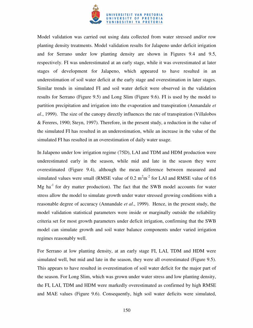
150

Model validation was carried out using data collected from water stressed and/or row

planting density treatments. Model validation results for Jalapeno under deficit irrigation

and for Serrano under low planting density are shown in Figures 9.4 and 9.5,

respectively. FI was underestimated at an early stage, while it was overestimated at later

stages of development for Jalapeno, which appeared to have resulted in an

underestimation of soil water deficit at the early stage and overestimation in later stages.

Similar trends in simulated FI and soil water deficit were observed in the validation

results for Serrano (Figure 9.5) and Long Slim (Figure 9.6). FI is used by the model to

partition precipitation and irrigation into the evaporation and transpiration (Annandale et

al., 1999). The size of the canopy directly influences the rate of transpiration (Villalobos

& Fereres, 1990; Steyn, 1997). Therefore, in the present study, a reduction in the value of

the simulated FI has resulted in an underestimation, while an increase in the value of the

simulated FI has resulted in an overestimation of daily water usage.

In Jalapeno under low irrigation regime (75D), LAI and TDM and HDM production were

underestimated early in the season, while mid and late in the season they were

overestimated (Figure 9.4), although the mean difference between measured and

simulated values were small (RMSE value of 0.2 m2m-2 for LAI and RMSE value of 0.6

Mg ha-1 for dry matter production). The fact that the SWB model accounts for water

stress allow the model to simulate growth under water stressed growing conditions with a

reasonable degree of accuracy (Annandale et al., 1999). Hence, in the present study, the

model validation statistical parameters were inside or marginally outside the reliability

criteria set for most growth parameters under deficit irrigation, confirming that the SWB

model can simulate growth and soil water balance components under varied irrigation

regimes reasonably well.

For Serrano at low planting density, at an early stage FI, LAI, TDM and HDM were

simulated well, but mid and late in the season, they were all overestimated (Figure 9.5).

This appears to have resulted in overestimation of soil water deficit for the major part of

the season. For Long Slim, which was grown under water stress and low planting density,

the FI, LAI, TDM and HDM were markedly overestimated as confirmed by high RMSE

and MAE values (Figure 9.6). Consequently, high soil water deficits were simulated,

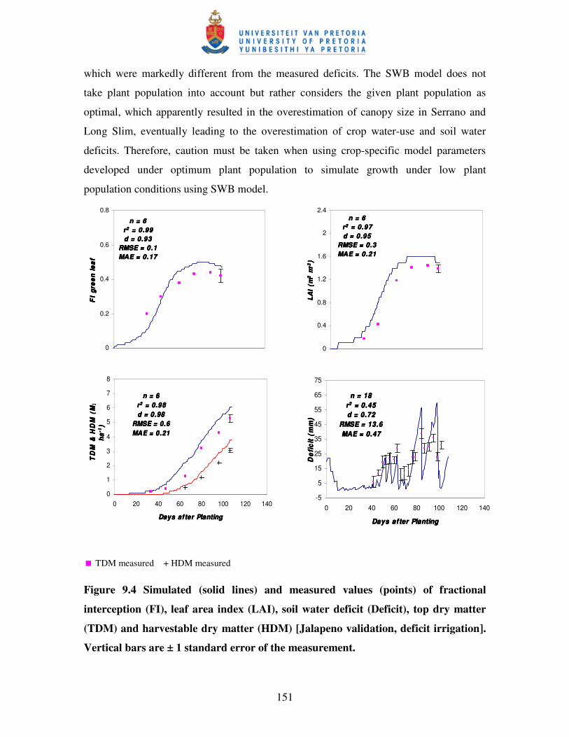
151

which were markedly different from the measured deficits. The SWB model does not

take plant population into account but rather considers the given plant population as

optimal, which apparently resulted in the overestimation of canopy size in Serrano and

Long Slim, eventually leading to the overestimation of crop water-use and soil water

deficits. Therefore, caution must be taken when using crop-specific model parameters

developed under optimum plant population to simulate growth under low plant

population conditions using SWB model.

n = 6n = 6n = 6n = 6rrrr2222 = 0.99 = 0.99 = 0.99 = 0.99d = 0.93d = 0.93d = 0.93d = 0.93


0

0.2

0.4

0.6

0.8

FI

gre

en l

eaf

FI

gre

en l

eaf

FI

gre

en l

eaf

FI

gre

en l

eaf

n = 6n = 6n = 6n = 6rrrr2222 = 0.98 = 0.98 = 0.98 = 0.98d = 0.98d = 0.98d = 0.98d = 0.98


0

1

2

3

4

5

6

7

8

0 20 40 60 80 100 120 140


TD

M &

HD

M (

Mg

T

DM

& H

DM

(M

g

TD

M &

HD

M (

Mg

T

DM

& H

DM

(M

g

haha haha

-1-1 -1-1)) ))

n = 6n = 6n = 6n = 6rrrr2222 = 0.97 = 0.97 = 0.97 = 0.97d = 0.95d = 0.95d = 0.95d = 0.95


0

0.4

0.8

1.2

1.6

2

2.4

LAI

(mLA

I (m

LAI

(mLA

I (m

22 22 m m m m

-2-2 -2-2)) ))

n = 18n = 18n = 18n = 18rrrr2222 = 0.45 = 0.45 = 0.45 = 0.45d = 0.72d = 0.72d = 0.72d = 0.72


-5

5

15

25

35

45

55

65

75

0 20 40 60 80 100 120 140


De

fic

it (

mm

)D

efi

cit

(m

m)

De

fic

it (

mm

)D

efi

cit

(m

m)




(TDM) and harvestable dry matter (HDM) [Jalapeno validation, deficit irrigation].

Vertical bars are ± 1 standard error of the measurement.

152

n = 6n = 6n = 6n = 6rrrr2222 = 0.95 = 0.95 = 0.95 = 0.95d = 0.96d = 0.96d = 0.96d = 0.96


0

0.1

0.2

0.3

0.4

0.5

0.6

0.7

0.8F

I g

reen

lea

fF

I g

reen

lea

fF

I g

reen

lea

fF

I g

reen

lea

f

n = 6n = 6n = 6n = 6rrrr2222 = 0.98 = 0.98 = 0.98 = 0.98d = 0.96d = 0.96d = 0.96d = 0.96


0

1

2

3

4

5

6

7

8

0 20 40 60 80 100 120 140


TD

M &

HD

M (

Mg

TD

M &

HD

M (

Mg

TD

M &

HD

M (

Mg

TD

M &

HD

M (

Mg

haha haha

-1-1 -1-1)) ))

n = 6n = 6n = 6n = 6rrrr2222 = 0.97 = 0.97 = 0.97 = 0.97d = 0.93d = 0.93d = 0.93d = 0.93


0

0.4

0.8

1.2

1.6

2

2.4

LAI

(mLA

I (m

LAI

(mLA

I (m

22 22 m m m m

-2-2 -2-2)) ))

n = 13n = 13n = 13n = 13rrrr2222 = 0.53 = 0.53 = 0.53 = 0.53d = 0.78d = 0.78d = 0.78d = 0.78


-5

5

15

25

35

45

55

65

75

0 20 40 60 80 100 120 140


De

fic

it (

mm

)D

efi

cit

(m

m)

De

fic

it (

mm

)D

efi

cit

(m

m)




(TDM) and harvestable dry matter (HDM) [Serrano validation, low density

planting]. Vertical bars are ± 1 standard error of the measurement.

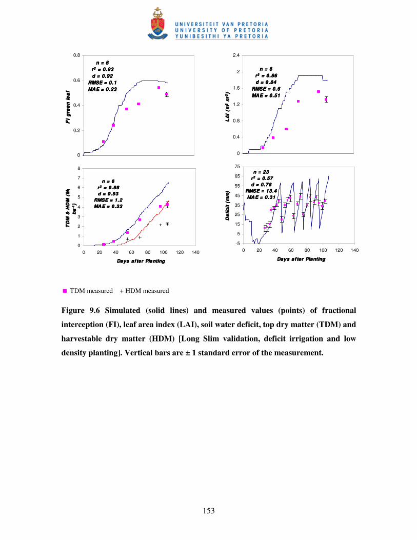
153

n = 6n = 6n = 6n = 6rrrr2222 = 0.93 = 0.93 = 0.93 = 0.93d = 0.92d = 0.92d = 0.92d = 0.92


0

0.2

0.4

0.6

0.8

FI

gre

en

lea

fF

I g

ree

n le

af

FI

gre

en

lea

fF

I g

ree

n le

af

n = 6n = 6n = 6n = 6rrrr2222 = 0.98 = 0.98 = 0.98 = 0.98d = 0.93d = 0.93d = 0.93d = 0.93


0

1

2

3

4

5

6

7

8

0 20 40 60 80 100 120 140


TD

M &

HD

M (

Mg

T

DM

& H

DM

(M

g

TD

M &

HD

M (

Mg

T

DM

& H

DM

(M

g

ha

ha

haha

-1-1 -1-1)) ))

n = 6n = 6n = 6n = 6rrrr2222 = 0.86 = 0.86 = 0.86 = 0.86d = 0.84d = 0.84d = 0.84d = 0.84


0

0.4

0.8

1.2

1.6

2

2.4

LA

I (m

LA

I (m

LA

I (m

LA

I (m

22 22 m m m m

-2-2 -2-2)) ))

n = 23n = 23n = 23n = 23 r r r r2222 = 0.57 = 0.57 = 0.57 = 0.57d = 0.76d = 0.76d = 0.76d = 0.76


-5

5

15

25

35

45

55

65

75

0 20 40 60 80 100 120 140


De

fic

it (

mm

)D

efi

cit

(m

m)

De

fic

it (

mm

)D

efi

cit

(m

m)



interception (FI), leaf area index (LAI), soil water deficit, top dry matter (TDM) and

harvestable dry matter (HDM) [Long Slim validation, deficit irrigation and low

density planting]. Vertical bars are ± 1 standard error of the measurement.

154

9.4 CONCLUSIONS

A database of crop-specific model parameters was generated for three South African

cultivars (Jalapeno, Serrano and Long Slim). The cultivars represent a wide range of

growth habits and fruiting characteristics. The SWB model was successfully

calibrated and validated for these cultivars for several growth parameters, and the soil

water deficit to field capacity was predicted with an accuracy that is sufficient for

irrigation scheduling. Validation simulations were inside or marginally outside the

reliability criteria for deficit irrigation treatments, confirming that the SWB model can

simulate growth and soil water balance components under varied irrigation regimes

reasonably well. However, caution must be exercised when using crop-specific model

parameters that are developed for optimum plant population conditions to simulate

growth under low planting populations, as most of the validation simulations were

outside the reliability criteria imposed for Long Slim under these conditions.

The model could be improved to account for the effects of plant population on

important crop-specific model parameters such as the canopy radiation extinction

coefficient, by setting up experiments that investigate the effect of different plant

populations on crop-specific model parameters.

155

CHAPTER 10

PREDICTING CROP WATER REQUIREMENTS FOR

HOT PEPPER CULTIVAR MAREKO FANA AT

DIFFERENT LOCATIONS IN ETHIOPIA USING THE

SOIL WATER BALANCE MODEL

Abstract Hot pepper is an important cash crop in Ethiopia. Irrigation is a standard practice in

hot pepper production. In the absence of real-time climate and crop data, know-how

and computing facilities, there is a need to generate semi-flexible irrigation schedules

to assist irrigators. Irrigation schedules and water requirements for growing Mareko

Fana in five hot pepper growing regions of Ethiopia were determined using crop-

specific model parameters determined for cultivar Mareko Fana, long term climate,

soil and management data.

Simulated irrigation requirements for hot pepper cultivar Mareko Fana production

ranged between 517 mm at Melkassa and 775 mm at Alemaya. The longest simulated

average irrigation interval was observed for Alemaya (9 days), while the lowest was

observed for Bako (6 days). The depth of irrigation ranged from 35 mm in Zeway to

28 mm in Bako. The difference in climatic variables and soil types among the sites for

which this study was done to influences the timing and depth of irrigation events.

Keywords: Ethiopia, hot pepper, irrigation calendars, SWB model, irrigation

requirements

156

10.1 INTRODUCTION

Irrigation agriculture in Ethiopia is in its infancy stage, and those irrigation regimes

currently existing in different schemes across the country were not monitored for the

past several years (Geremew, 2008). The same author indicated that the irrigation

regimes in Godino (Ethiopia) in potato and onion performed poorer than the scientific

methods, SWB and re-filling soil water deficit to field capacity as monitored by

neutron water meter. This, in part, can be attributed for the low water-use efficiency

of crops under traditional irrigation schemes.

Water-use efficiency can be improved through practicing irrigation scheduling.

Irrigation scheduling is the practice of applying the right amount of water at the right

time for plant production. Irrigation scheduling is traditionally based on soil water

measurement, where the soil water status is measured directly to determine the need

for irrigation. Examples are monitoring soil water by means of tensiometers (Cassel &

Klute, 1986), electrical resistance and heat dissipation soil water sensors (Jovanovic &

Annandale, 1997), or neutron water meters (Gardner, 1986). A potential problem with

soil water based approaches is that many features of the plant’s physiology respond

directly to changes in water status in the plant tissues, rather than to changes in the

bulk soil water content. Apart from this, soil heterogeneity requires many sensors,

selecting a position that is representative of the root zone is difficult, and sensors

usually measure water status at root zone (Jones, 2004). The availability and lack of

know-how discourage adoption of this approach by poor farmers.

The second approach is to base irrigation scheduling decisions on plant response,

rather than on direct measurements of soil water status (Bordovsky et al., 1974;

O’Toole et al., 1984). However, the majority of systems require instruments beyond

the reach of ordinary farmers. High technical know-how and the time required to use

these instruments usually discourage their ready application. Furthermore, most

physiological indices of plant water stress (leaf water potential, leaf water content,

diffusion resistance, canopy temperature) not only involve measurements that are

complex, time consuming and difficult to integrate, but are also subject to errors

(Jones, 2004). On top of this, if our measurement target is only one aspect (plant) of

the soil-plant-atmosphere continuum, it may be difficult to estimate plant water

requirements realistically, as the system is very interrelated.

157

The third option is soil water balance calculations, where the soil water status is

estimated by calculation using a water balance approach in which the change in soil

water over a period is given by the difference between the inputs (irrigation plus

precipitation) and losses (runoff plus drainage plus evapotranspiration) (Allen et al.,

1998). The input parameters are easy to measure using conventional instruments like

rain gauge for rainfall and irrigation, and water meters for irrigation. The runoff and

drainage could be either estimated from soil parameters or directly measured in situ or

would be assumed negligible based on soil condition and water supply.

Evapotranspiration can be estimated from climatic variables (Doorenbos & Pruitt,

1992; Allen et al., 1998) or from pan evaporation (Elliades, 1988; Sezen et al., 2006).

Currently, application of the soil water balance method for irrigation scheduling is

growing because of better understanding of the soil-plant-atmosphere continuum and

the ready availability of computer facilities to compute complex equations. Various

computer software aids are available that utilize soil, plant, atmosphere and

management data to estimate plant water requirements. Annandale et al. (1999)

demonstrated, on many fruit, vegetable and field crops, SWB model to predict the

plant water requirements realistically. Elsewhere, different authors (Smith, 1992;

Allen et al., 1998) employing similar principles working on different crops under

different conditions came up with similar conclusions. Furthermore, collecting and

analyzing the long-term climatic data help to understand the evaporative demand of

the atmosphere and the potential water supply of a region in a growing season for

better water management (Smith, 2000). This information coupled with crop, soil and

management data enables us to generate irrigation calendars using computer software.

An irrigation calendar is a simple chart or guideline that indicate when and how much

to irrigate. It is generated by software using data of long term climatic, soil, irrigation

type and crop species, and management. It can be made flexible by including real-

time soil water and rainfall measurement in the calculation of water requirements of a

crop. Work by Hill & Allen (1996) in Pakistan and USA, and by Raes et al. (2000) in

Tunisia have shown a semi-flexible irrigation calendar facilitated the adoption of

irrigation scheduling due to less technical knowledge required in understanding and

employing the irrigation scheduling. In this regard, the SWB model is equipped with

the necessary facilities to enable the development of irrigation calendars and water

158

requirements of specific crops from climatic, soil, crop and management data. The

objectives of the present study were:

1. to estimate the water requirements of hot pepper (cultivar Mareko Fana) and

evaluate its productivity across five ecological regions of Ethiopia using the SWB

model, and

2. to establish irrigation schedules of hot pepper for five ecological regions of

Ethiopia using the SWB model and long term weather data.

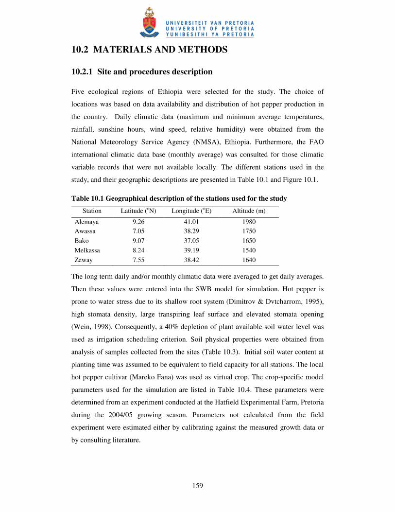
159


10.2.1 Site and procedures description

Five ecological regions of Ethiopia were selected for the study. The choice of

locations was based on data availability and distribution of hot pepper production in

the country. Daily climatic data (maximum and minimum average temperatures,

rainfall, sunshine hours, wind speed, relative humidity) were obtained from the

National Meteorology Service Agency (NMSA), Ethiopia. Furthermore, the FAO

international climatic data base (monthly average) was consulted for those climatic

variable records that were not available locally. The different stations used in the

study, and their geographic descriptions are presented in Table 10.1 and Figure 10.1.

Table 10.1 Geographical description of the stations used for the study

Station Latitude (oN) Longitude (oE) Altitude (m)

Alemaya 9.26 41.01 1980 Awassa 7.05 38.29 1750 Bako 9.07 37.05 1650 Melkassa 8.24 39.19 1540 Zeway 7.55 38.42 1640

The long term daily and/or monthly climatic data were averaged to get daily averages.

Then these values were entered into the SWB model for simulation. Hot pepper is

prone to water stress due to its shallow root system (Dimitrov & Dvtcharrom, 1995),

high stomata density, large transpiring leaf surface and elevated stomata opening

(Wein, 1998). Consequently, a 40% depletion of plant available soil water level was

used as irrigation scheduling criterion. Soil physical properties were obtained from

analysis of samples collected from the sites (Table 10.3). Initial soil water content at

planting time was assumed to be equivalent to field capacity for all stations. The local

hot pepper cultivar (Mareko Fana) was used as virtual crop. The crop-specific model

parameters used for the simulation are listed in Table 10.4. These parameters were

determined from an experiment conducted at the Hatfield Experimental Farm, Pretoria

during the 2004/05 growing season. Parameters not calculated from the field

experiment were estimated either by calibrating against the measured growth data or

by consulting literature.

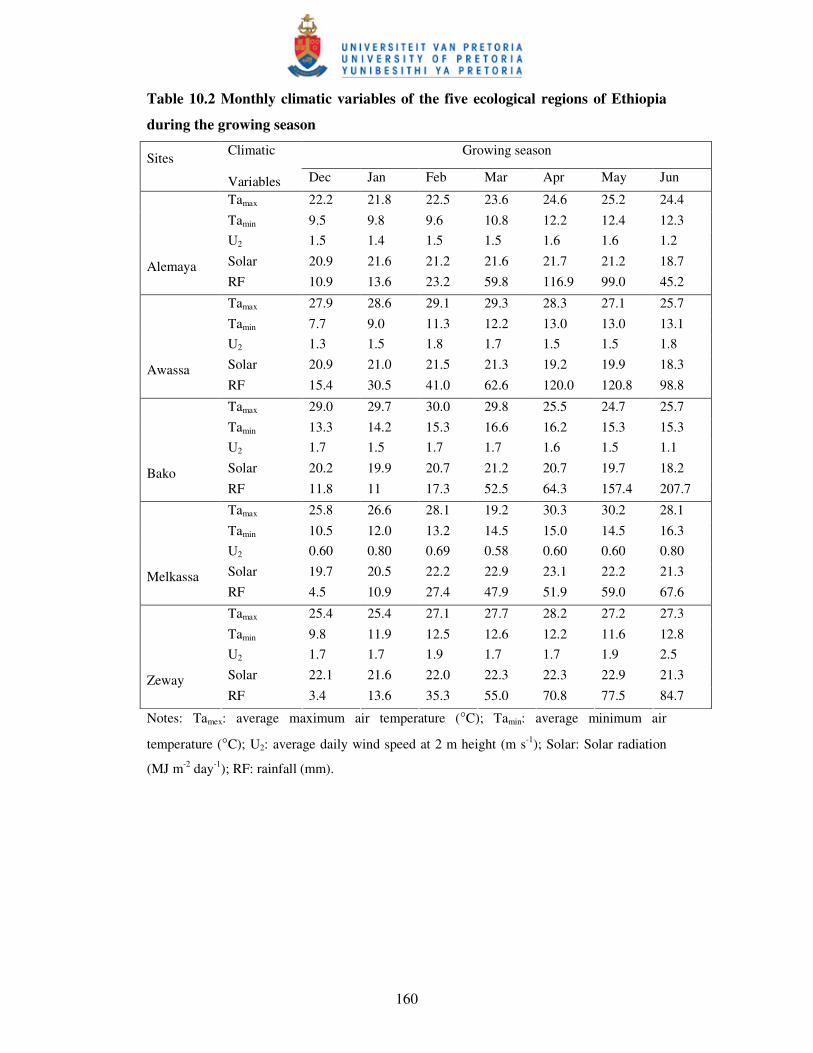
160

Table 10.2 Monthly climatic variables of the five ecological regions of Ethiopia

during the growing season

Growing season Sites Climatic

Variables Dec Jan Feb Mar Apr May Jun

Tamax 22.2 21.8 22.5 23.6 24.6 25.2 24.4 Tamin 9.5 9.8 9.6 10.8 12.2 12.4 12.3 U2 1.5 1.4 1.5 1.5 1.6 1.6 1.2 Solar 20.9 21.6 21.2 21.6 21.7 21.2 18.7

Alemaya RF 10.9 13.6 23.2 59.8 116.9 99.0 45.2


Awassa RF 15.4 30.5 41.0 62.6 120.0 120.8 98.8


Bako RF 11.8 11 17.3 52.5 64.3 157.4 207.7


Melkassa RF 4.5 10.9 27.4 47.9 51.9 59.0 67.6


Zeway RF 3.4 13.6 35.3 55.0 70.8 77.5 84.7

Notes: Tamex: average maximum air temperature (°C); Tamin: average minimum air

temperature (°C); U2: average daily wind speed at 2 m height (m s-1); Solar: Solar radiation

(MJ m-2 day-1); RF: rainfall (mm).

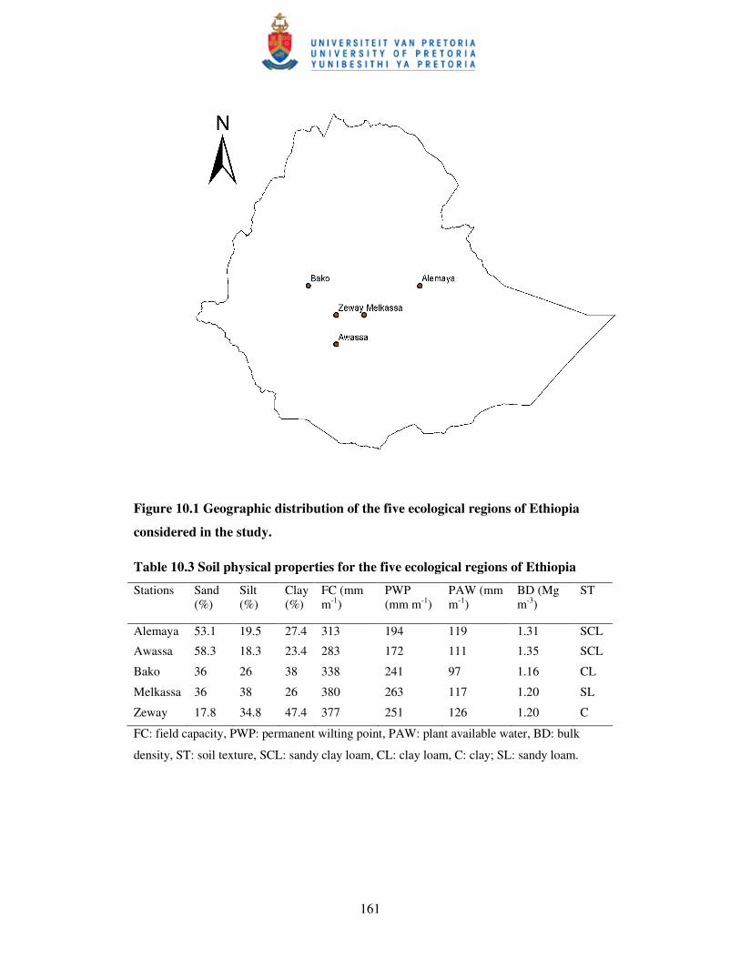
161

Figure 10.1 Geographic distribution of the five ecological regions of Ethiopia

considered in the study.

Table 10.3 Soil physical properties for the five ecological regions of Ethiopia

Stations Sand (%)

Silt (%)

Clay (%)

FC (mm m-1)

PWP (mm m-1)

PAW (mm m-1)

BD (Mg m-3)

ST

Alemaya 53.1 19.5 27.4 313 194 119 1.31 SCL

Awassa 58.3 18.3 23.4 283 172 111 1.35 SCL

Bako 36 26 38 338 241 97 1.16 CL

Melkassa 36 38 26 380 263 117 1.20 SL

Zeway 17.8 34.8 47.4 377 251 126 1.20 C

FC: field capacity, PWP: permanent wilting point, PAW: plant available water, BD: bulk

density, ST: soil texture, SCL: sandy clay loam, CL: clay loam, C: clay; SL: sandy loam.

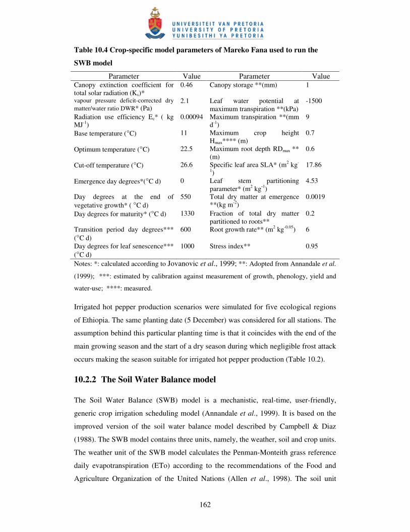
162

Table 10.4 Crop-specific model parameters of Mareko Fana used to run the

SWB model

Parameter Value Parameter Value Canopy extinction coefficient for total solar radiation (Ks)*

0.46 Canopy storage **(mm) 1

vapour pressure deficit-corrected dry matter/water ratio DWR* (Pa)

2.1 Leaf water potential at maximum transpiration **(kPa)

-1500

Radiation use efficiency Ec* ( kg MJ-1)

0.00094 Maximum transpiration **(mm d-1)

9

Base temperature (°C) 11 Maximum crop height Hmax**** (m)

0.7

Optimum temperature (°C) 22.5 Maximum root depth RDmax ** (m)

0.6

Cut-off temperature (°C) 26.6 Specific leaf area SLA* (m2 kg-

1) 17.86

Emergence day degrees*(°C d) 0 Leaf stem partitioning parameter* (m2 kg-1)

4.53

Day degrees at the end of vegetative growth* ( °C d)

550 Total dry matter at emergence **(kg m-2)

0.0019

Day degrees for maturity* (°C d) 1330 Fraction of total dry matter partitioned to roots**

0.2

Transition period day degrees*** (°C d)

600 Root growth rate** (m2 kg-0.05) 6

Day degrees for leaf senescence*** (°C d)

1000 Stress index** 0.95

Notes: *: calculated according to Jovanovic et al., 1999; **: Adopted from Annandale et al.

(1999); ***: estimated by calibration against measurement of growth, phenology, yield and

water-use; ****: measured.

Irrigated hot pepper production scenarios were simulated for five ecological regions

of Ethiopia. The same planting date (5 December) was considered for all stations. The

assumption behind this particular planting time is that it coincides with the end of the

main growing season and the start of a dry season during which negligible frost attack

occurs making the season suitable for irrigated hot pepper production (Table 10.2).

10.2.2 The Soil Water Balance model

The Soil Water Balance (SWB) model is a mechanistic, real-time, user-friendly,

generic crop irrigation scheduling model (Annandale et al., 1999). It is based on the

improved version of the soil water balance model described by Campbell & Diaz

(1988). The SWB model contains three units, namely, the weather, soil and crop units.

The weather unit of the SWB model calculates the Penman-Monteith grass reference

daily evapotranspiration (ETo) according to the recommendations of the Food and

Agriculture Organization of the United Nations (Allen et al., 1998). The soil unit

163

simulates the dynamics of soil water movement (runoff, interception, infiltration,

transpiration, soil water storage and evaporation) in order to quantify soil water

content. In the crop unit, the SWB model calculates crop dry matter accumulation in

direct proportion to vapour pressure deficit-corrected dry matter/water ratio (Tanner

& Sinclair, 1983). The crop unit also calculates radiation-limited growth (Monteith,

1977) and takes the lower of the two. This dry matter is partitioned to the roots, stems,

leaves and grains or fruits. Partitioning depends on phenology, calculated with

thermal time and modified by water stress.

Input data to run the model include site and crop characteristics. The site-specific data

include weather (daily maximum and minimum temperatures, solar radiation, wind

speed and vapour pressure), altitude, latitude, and hemisphere. In the absence of

measured data on solar radiation, wind speed, and vapour pressure; the model is

equipped with functions for estimating these parameters from available weather data

according to FAO 56 recommendation (Allen et al., 1998).

Soil input data such as the runoff curve number, drainage fraction and maximum

drainage rate, soil layer characteristics (thickness, volumetric soil water content at

field capacity and permanent wilting points, initial volumetric water content, and bulk

density) are also required to run the model.

The crop-specific model parameters required to run the growth model in the SWB

model includes canopy radiation extinction coefficient, vapour pressure deficit-

corrected dry matter/water ratio, radiation use efficiency, base temperature, optimum

temperature for crop growth, cut-off temperature, maximum crop height, day degrees

at the end of vegetative growth, day degrees for maturity, transition period day

degrees, day degrees for leaf senescence, maximum root depth, fraction of total dry

matter translocated to heads, canopy storage, leaf potential at maximum transpiration,

maximum transpiration, specific model leaf area, leaf-stem partitioning parameter,

total dry matter at emergence, fraction of total dry matter partitioned to roots, root

growth rate and stress index.

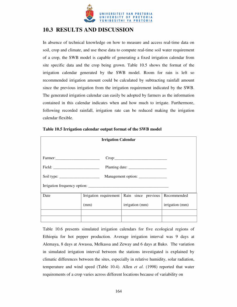
164


In absence of technical knowledge on how to measure and access real-time data on

soil, crop and climate, and use these data to compute real-time soil water requirement

of a crop, the SWB model is capable of generating a fixed irrigation calendar from

site specific data and the crop being grown. Table 10.5 shows the format of the

irrigation calendar generated by the SWB model. Room for rain is left so

recommended irrigation amount could be calculated by subtracting rainfall amount

since the previous irrigation from the irrigation requirement indicated by the SWB.

The generated irrigation calendar can easily be adopted by farmers as the information

contained in this calendar indicates when and how much to irrigate. Furthermore,

following recorded rainfall, irrigation rate can be reduced making the irrigation

calendar flexible.

Table 10.5 Irrigation calendar output format of the SWB model

Irrigation Calendar

Farmer:______________________ Crop:__________________________

Field: _______________________ Planting date: ___________________

Soil type: ____________________ Management option: ______________

Irrigation frequency option: ________________________________________

Date Irrigation requirement

(mm)

Rain since previous

irrigation (mm)

Recommended

irrigation (mm)

Table 10.6 presents simulated irrigation calendars for five ecological regions of

Ethiopia for hot pepper production. Average irrigation interval was 9 days at

Alemaya, 8 days at Awassa, Melkassa and Zeway and 6 days at Bako. The variation

in simulated irrigation interval between the stations investigated is explained by

climatic differences between the sites, especially in relative humidity, solar radiation,

temperature and wind speed (Table 10.4). Allen et al. (1998) reported that water

requirements of a crop varies across different locations because of variability on

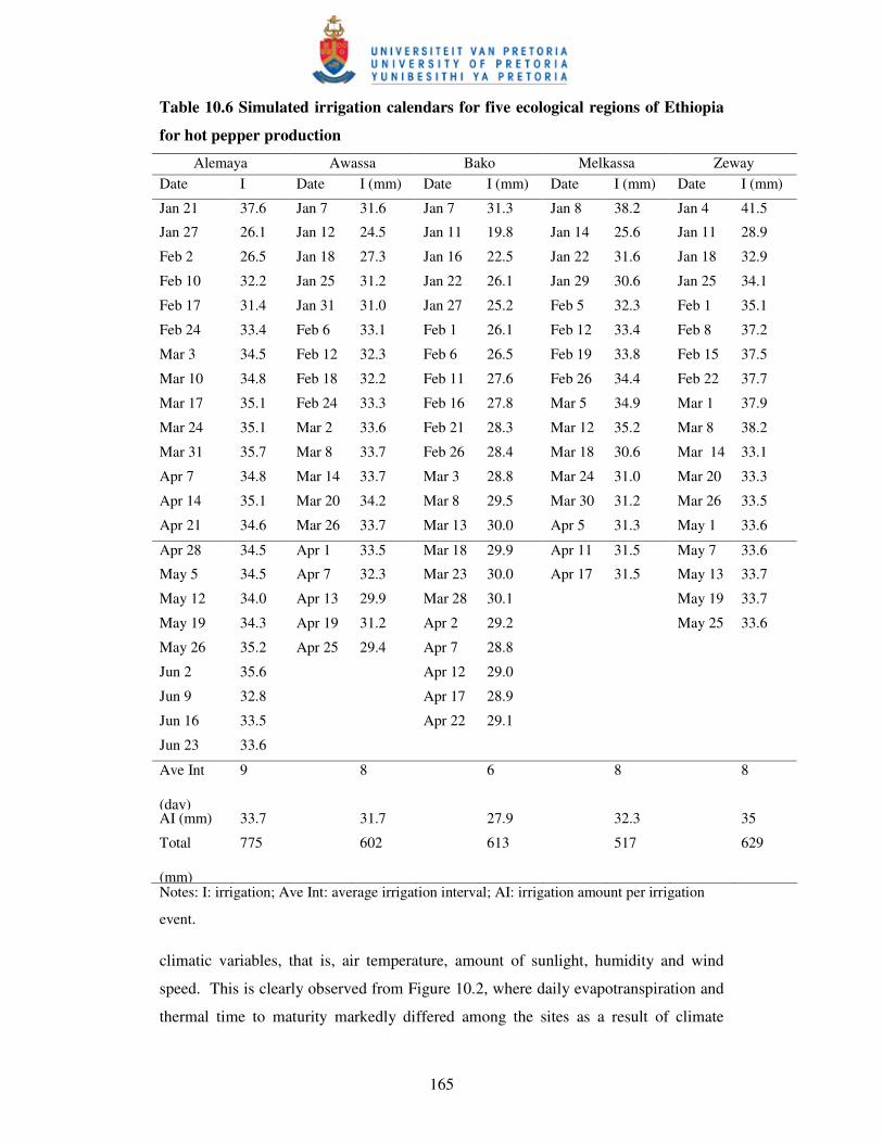
165

Table 10.6 Simulated irrigation calendars for five ecological regions of Ethiopia

for hot pepper production

Alemaya Awassa Bako Melkassa Zeway Date I Date I (mm) Date I (mm) Date I (mm) Date I (mm)

Jan 21 37.6 Jan 7 31.6 Jan 7 31.3 Jan 8 38.2 Jan 4 41.5

Jan 27 26.1 Jan 12 24.5 Jan 11 19.8 Jan 14 25.6 Jan 11 28.9

Feb 2 26.5 Jan 18 27.3 Jan 16 22.5 Jan 22 31.6 Jan 18 32.9

Feb 10 32.2 Jan 25 31.2 Jan 22 26.1 Jan 29 30.6 Jan 25 34.1

Feb 17 31.4 Jan 31 31.0 Jan 27 25.2 Feb 5 32.3 Feb 1 35.1

Feb 24 33.4 Feb 6 33.1 Feb 1 26.1 Feb 12 33.4 Feb 8 37.2

Mar 3 34.5 Feb 12 32.3 Feb 6 26.5 Feb 19 33.8 Feb 15 37.5

Mar 10 34.8 Feb 18 32.2 Feb 11 27.6 Feb 26 34.4 Feb 22 37.7

Mar 17 35.1 Feb 24 33.3 Feb 16 27.8 Mar 5 34.9 Mar 1 37.9

Mar 24 35.1 Mar 2 33.6 Feb 21 28.3 Mar 12 35.2 Mar 8 38.2

Mar 31 35.7 Mar 8 33.7 Feb 26 28.4 Mar 18 30.6 Mar 14 33.1

Apr 7 34.8 Mar 14 33.7 Mar 3 28.8 Mar 24 31.0 Mar 20 33.3

Apr 14 35.1 Mar 20 34.2 Mar 8 29.5 Mar 30 31.2 Mar 26 33.5

Apr 21 34.6 Mar 26 33.7 Mar 13 30.0 Apr 5 31.3 May 1 33.6

Apr 28 34.5 Apr 1 33.5 Mar 18 29.9 Apr 11 31.5 May 7 33.6

May 5 34.5 Apr 7 32.3 Mar 23 30.0 Apr 17 31.5 May 13 33.7

May 12 34.0 Apr 13 29.9 Mar 28 30.1 May 19 33.7

May 19 34.3 Apr 19 31.2 Apr 2 29.2 May 25 33.6

May 26 35.2 Apr 25 29.4 Apr 7 28.8

Jun 2 35.6 Apr 12 29.0

Jun 9 32.8 Apr 17 28.9

Jun 16 33.5 Apr 22 29.1

Jun 23 33.6

Ave Int

(day)

9 8 6 8 8

AI (mm) 33.7 31.7 27.9 32.3 35

Total

(mm)

775 602 613 517 629

Notes: I: irrigation; Ave Int: average irrigation interval; AI: irrigation amount per irrigation

event.

climatic variables, that is, air temperature, amount of sunlight, humidity and wind

speed. This is clearly observed from Figure 10.2, where daily evapotranspiration and

thermal time to maturity markedly differed among the sites as a result of climate

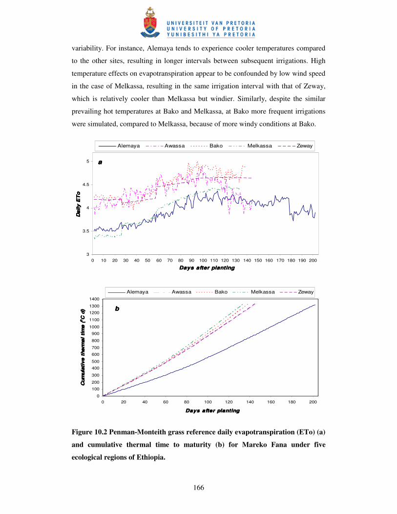
166

variability. For instance, Alemaya tends to experience cooler temperatures compared

to the other sites, resulting in longer intervals between subsequent irrigations. High

temperature effects on evapotranspiration appear to be confounded by low wind speed

in the case of Melkassa, resulting in the same irrigation interval with that of Zeway,

which is relatively cooler than Melkassa but windier. Similarly, despite the similar

prevailing hot temperatures at Bako and Melkassa, at Bako more frequent irrigations

were simulated, compared to Melkassa, because of more windy conditions at Bako.

aaaa

3

3.5

4

4.5

5

0 10 20 30 40 50 60 70 80 90 100 110 120 130 140 150 160 170 180 190 200


Dai

ly E

To

Dai

ly E

To

Dai

ly E

To

Dai

ly E

To

Alemaya Awassa Bako Melkassa Zeway

bbbb

0

100

200

300

400

500

600

700

800

900

1000

1100

1200

1300

1400

0 20 40 60 80 100 120 140 160 180 200


Cum

ulat

ive

ther

mal

tim

e (

Cum

ulat

ive

ther

mal

tim

e (

Cum

ulat

ive

ther

mal

tim

e (

Cum

ulat

ive

ther

mal

tim

e (oo oo

C d

)C

d)

C d

)C

d)

Alemaya Awassa Bako Melkassa Zeway

Figure 10.2 Penman-Monteith grass reference daily evapotranspiration (ETo) (a)

and cumulative thermal time to maturity (b) for Mareko Fana under five

ecological regions of Ethiopia.

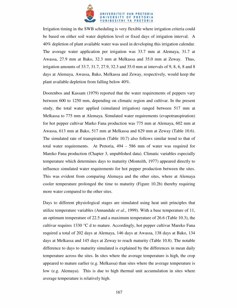
167

Irrigation timing in the SWB scheduling is very flexible where irrigation criteria could

be based on either soil water depletion level or fixed days of irrigation interval. A

40% depletion of plant available water was used in developing this irrigation calendar.

The average water application per irrigation was 33.7 mm at Alemaya, 31.7 at

Awassa, 27.9 mm at Bako, 32.3 mm at Melkassa and 35.0 mm at Zeway. Thus,

irrigation amounts of 33.7, 31.7, 27.9, 32.3 and 35.0 mm at intervals of 9, 8, 6, 8 and 8

days at Alemaya, Awassa, Bako, Melkassa and Zeway, respectively, would keep the

plant available depletion from falling below 40%.

Doorenbos and Kassam (1979) reported that the water requirements of peppers vary

between 600 to 1250 mm, depending on climatic region and cultivar. In the present

study, the total water applied (simulated irrigation) ranged between 517 mm at

Melkassa to 775 mm at Alemaya. Simulated water requirements (evapotranspiration)

for hot pepper cultivar Marko Fana production was 775 mm at Alemaya, 602 mm at

Awassa, 613 mm at Bako, 517 mm at Melkassa and 629 mm at Zeway (Table 10.6).

The simulated rate of transpiration (Table 10.7) also follows similar trend to that of

total water requirements. At Pretoria, 494 - 586 mm of water was required for

Mareko Fana production (Chapter 3, unpublished data). Climatic variables especially

temperature which determines days to maturity (Monteith, 1977) appeared directly to

influence simulated water requirements for hot pepper production between the sites.

This was evident from comparing Alemaya and the other sites, where at Alemaya

cooler temperature prolonged the time to maturity (Figure 10.2b) thereby requiring

more water compared to the other sites.

Days to different physiological stages are simulated using heat unit principles that

utilize temperature variables (Annandale et al., 1999). With a base temperature of 11,

an optimum temperature of 22.5 and a maximum temperature of 26.6 (Table 10.3), the

cultivar requires 1330 °C d to mature. Accordingly, hot pepper cultivar Mareko Fana

required a total of 202 days at Alemaya, 146 days at Awassa, 138 days at Bako, 134

days at Melkassa and 145 days at Zeway to reach maturity (Table 10.8). The notable

difference to days to maturity simulated is explained by the differences in mean daily

temperature across the sites. In sites where the average temperature is high, the crop

appeared to mature earlier (e.g. Melkassa) than sites where the average temperature is

low (e.g. Alemaya). This is due to high thermal unit accumulation in sites where

average temperature is relatively high.

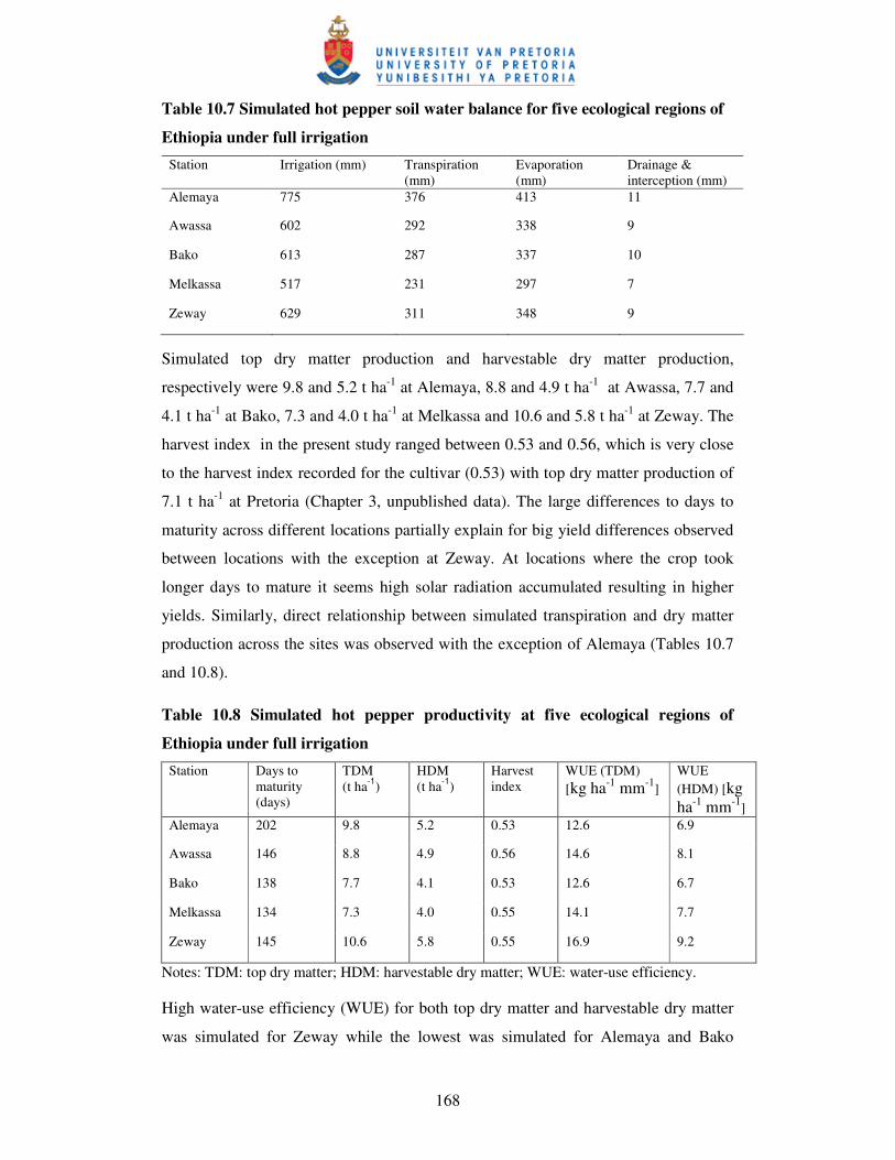
168

Table 10.7 Simulated hot pepper soil water balance for five ecological regions of

Ethiopia under full irrigation Station Irrigation (mm) Transpiration

(mm) Evaporation (mm)

Drainage & interception (mm)

Alemaya 775 376 413 11

Awassa 602 292 338 9

Bako 613 287 337 10

Melkassa 517 231 297 7

Zeway 629 311 348 9

Simulated top dry matter production and harvestable dry matter production,

respectively were 9.8 and 5.2 t ha-1 at Alemaya, 8.8 and 4.9 t ha-1 at Awassa, 7.7 and

4.1 t ha-1 at Bako, 7.3 and 4.0 t ha-1 at Melkassa and 10.6 and 5.8 t ha-1 at Zeway. The

harvest index in the present study ranged between 0.53 and 0.56, which is very close

to the harvest index recorded for the cultivar (0.53) with top dry matter production of

7.1 t ha-1 at Pretoria (Chapter 3, unpublished data). The large differences to days to

maturity across different locations partially explain for big yield differences observed

between locations with the exception at Zeway. At locations where the crop took

longer days to mature it seems high solar radiation accumulated resulting in higher

yields. Similarly, direct relationship between simulated transpiration and dry matter

production across the sites was observed with the exception of Alemaya (Tables 10.7

and 10.8).

Table 10.8 Simulated hot pepper productivity at five ecological regions of

Ethiopia under full irrigation Station Days to

maturity (days)

TDM (t ha-1)

HDM (t ha-1)

Harvest index

WUE (TDM) [kg ha-1 mm-1]

WUE (HDM) [kg ha-1 mm-1]

Alemaya 202 9.8 5.2 0.53 12.6 6.9

Awassa 146 8.8 4.9 0.56 14.6 8.1

Bako 138 7.7 4.1 0.53 12.6 6.7

Melkassa 134 7.3 4.0 0.55 14.1 7.7

Zeway 145 10.6 5.8 0.55 16.9 9.2

Notes: TDM: top dry matter; HDM: harvestable dry matter; WUE: water-use efficiency.

High water-use efficiency (WUE) for both top dry matter and harvestable dry matter

was simulated for Zeway while the lowest was simulated for Alemaya and Bako

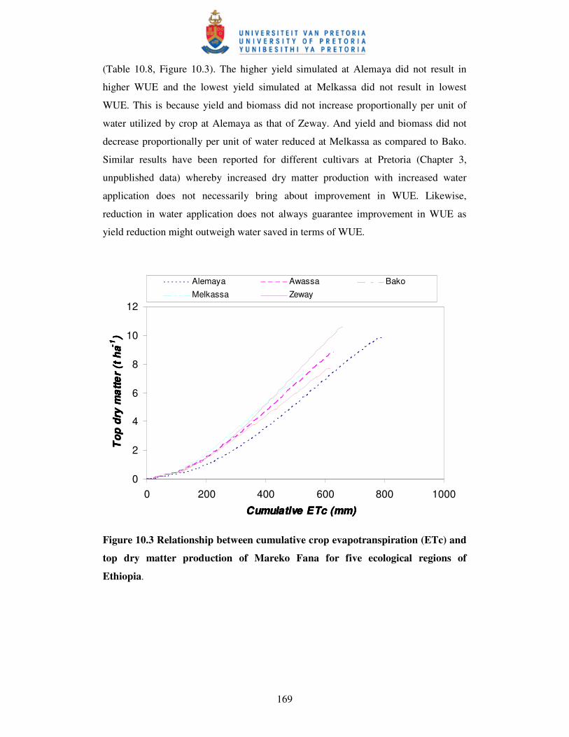
169

(Table 10.8, Figure 10.3). The higher yield simulated at Alemaya did not result in

higher WUE and the lowest yield simulated at Melkassa did not result in lowest

WUE. This is because yield and biomass did not increase proportionally per unit of

water utilized by crop at Alemaya as that of Zeway. And yield and biomass did not

decrease proportionally per unit of water reduced at Melkassa as compared to Bako.

Similar results have been reported for different cultivars at Pretoria (Chapter 3,

unpublished data) whereby increased dry matter production with increased water

application does not necessarily bring about improvement in WUE. Likewise,

reduction in water application does not always guarantee improvement in WUE as

yield reduction might outweigh water saved in terms of WUE.

0

2

4

6

8

10

12

0 200 400 600 800 1000

Cumulative ETc (mm)Cumulative ETc (mm)Cumulative ETc (mm)Cumulative ETc (mm)

Top

dry

mat

ter

(t h

aT

op d

ry m

atte

r (t

ha

Top

dry

mat

ter

(t h

aT

op d

ry m

atte

r (t

ha-1-1 -1-1

)) ))

Alemaya Awassa BakoMelkassa Zeway

Figure 10.3 Relationship between cumulative crop evapotranspiration (ETc) and

top dry matter production of Mareko Fana for five ecological regions of

Ethiopia.

170

10.4 CONCLUSIONS

Irrigation calendars and water requirements for hot pepper production at five

ecological regions of Ethiopia were established using the Soil Water Balance model.

Water balance, days to maturity and dry matter production were simulated, and WUE

and harvest index were calculated for the five ecological regions considered. The

highest simulated average irrigation interval observed was at Alemaya, while the

lowest was at Bako. There appeared marked variation in irrigation amount per

irrigation and total water requirements among the five ecological regions studied. The

variation in irrigation depth and interval across the different locations is due to

difference in climatic variables, that is, relative humidity, solar radiation, temperature

and wind speed. Temperature was used by the SWB model to simulate days to

maturity, and hence it appeared that where the average temperature is low, the crop

took a longer time to mature, which in turn contributed to high total water

requirements in the cooler environment. Differences in soil water holding capacity

also seems to contribute for variations in days between irrigation events

The generated irrigation calendars are simple to read and provide farmers with

important information pertaining to scheduling irrigation. Furthermore, the generated

irrigation calendar can be made flexible to account for rainfall, where

recommendation on irrigation amounts could be calculated by subtracting rainfall

amount since the previous irrigation from the irrigation requirement indicated by the

SWB. This type of irrigation calendar can be easily generated by the district Ministry

of Agriculture’s irrigation specialist and the calendar can be disseminated to farmers

using development agents working with the farmers. Owing to its simplicity, such

irrigation calendars is expected to be highly adoptable by farmers for aiding irrigation

scheduling.

171

CHAPTER 11

GENERAL CONCLUSIONS AND RECOMMENDATIONS

11.1 GENERAL CONCLUSIONS

Hot pepper is a warm season, high value cash crop, of which production is generally

confined to areas where water is often limiting. Since the crop is sensitive to water

stress irrigation is standard practice in hot pepper production. However, the amount of

water available for irrigation is declining consistently as a result of pressure from

other competing sectors (domestic, recreation, environmental and industrial uses).

Furthermore, excess water application of irrigation is one of the main reasons for

degradation of agricultural land through salinization. Hence there is a need to

improve irrigation management and water-use efficiency in crop production.

Furthermore, with hot pepper being a high value and labour-intensive cash crop, with

high production costs, it is necessary to devise means of decreasing the cost of

production. Irrigation as a tactical tool to increase productivity of hot pepper is

recommended, because irrigation improves yield by its direct effect of mitigating

water stress, and encourages farmers to invest in inputs such as fertilizers and

improved cultivars.

Irrigation scheduling and deficit irrigation form part of proper irrigation management

that are crucial for improving the water-use efficiency of hot pepper. Irrigation

scheduling improves water-use efficiency by enabling an irrigator to use the right

amount of water at the right time for plant production. Likewise, deficit irrigation, the

deliberate and systematic under-irrigation of crops, increases the water-use efficiency

of a crop by reducing evaporation, but maintaining yield that is comparable to a fully

irrigated crop. It can also conserve water and minimize leaching of nutrients and

pesticides to groundwater. Furthermore, understanding the variability of cultivar

response to different irrigation regimes, and the influence of cultural practices such as

row spacing on hot pepper response to irrigation are crucial in improving the water-

use efficiency of hot pepper.

172

Accordingly, a series of field, rainshelter, growth cabinet and modelling studies were

conducted: to investigate hot pepper response to different irrigation regimes and row

spacings; to generate FAO-type crop factors and crop-specific model parameters; to

calibrate and validate the Soil Water Balance (SWB) model, to develop irrigation

calendars, and estimate water requirements of hot pepper under different growing

conditions.

Canopy size and its configuration is an important crop characteristic that determines

efficiency of radiation capture by a crop. This plant growth attribute is quantified

using plant parameters such as LAI, SLA and FI, which are influenced by cultivar and

growing conditions. In the present studies, the effects of row spacing, irrigation

regime and cultivar differences on these parameters were investigated. Irrigation

regime and row spacing significantly affected FI. Narrow row spacing significantly

increased LAI, and although the effect was small, an increasing trend in LAI was

observed for the high irrigation regime. The influence of irrigation regime and row

spacing on SLA was inconclusive, while marked variation in SLA was observed

among the cultivars. The higher solar radiation interception in the narrow row

spacings is attributed to a more even leaf distribution than in the wider row. A

reduction in FI due to water stress is attributed to the corresponding reduction in LAI

as a result of water stress.

Water-use and water-use efficiency, in a crop are important variables employed to

quantify the water usage and water-use efficiency of a crop. The water requirements

of peppers vary between 600 to 1250 mm, depending on region, climate and cultivar

(Doorenbos & Kassam, 1979). Seasonal water-use, in the open field experiment,

across cultivars varied between 516 mm for Jalapeno and 675 mm for Malaga in the

well-watered treatment (25D). Under severe water stress (75D), the seasonal water-

use ranged from 430 mm for Jalapeno and 532 mm for Malaga. The variation in

water-use among the cultivars is mainly attributed to the length of the growing season.

The seasonal water-use in the rainshelter experiment varied between 539 mm for the

well-watered and 369 mm for the water-stressed treatments. The corresponding

average irrigation interval was three days for well-irrigated and 10 days for the water-

stressed treatments.

173

Variable WUE results were reported for pepper with different irrigation regimes. In

the present studies, WUE was improved for high density plantings, but remained

unaffected by irrigation regime. WUE did not improve with a reduced irrigation

regime, as the water saved was overshadowed by yield loss. High WUE were

observed due to high plant density. This is attributed to the significant improvement in

fresh and dry fruit mass as well as top dry matter produced due to high plant density.

The WUE in terms of fresh and dry fruit yields were significantly influenced by

cultivar, but WUE for top dry matter production was not cultivar dependent. The

marked variation in WUE among cultivars is attributed to their differences in time to

maturity and harvest index.

Fruit yield in hot pepper is a function of total dry matter production and harvest index.

Fruit yield in hot pepper can also be related to fruit number per plant and average fruit

mass. High irrigation regimes and high plant density significantly increased fresh and

dry fruit yields. High irrigation regimes significantly improved the top, and stem dry

matter, fruit number per plant and assimilate partitioned to fruit in both the rainshelter

and open field experiments. Leaf dry matter and average fruit mass were not affected

by irrigation regime in both the rainshelter and open field experiments. Variable

results were obtained for assimilates partitioned to stems and leaves between the

rainshelter and open field experiments as the irrigation regime changed.

The marked improvement in dry fruit yield by the higher irrigation regime was

attributed to the corresponding significant increase in harvest index, fruit number and

top dry mass observed under the high irrigation regime. The marked yield differences

between the 25D and 55D treatments, in the rainshelter experiment, showed that mild

water stress could cause substantial yield loss in hot pepper, confirming the sensitivity

of hot pepper to water stress. Thus, it is recommended to maintain the depletion of

plant available water between 20-25% for maximum yield. However, where the cost

of fresh water is high, further research is recommended to establish optimal irrigation

regimes between 25 and 55% depletion of plant available water. Furthermore,

research that seeks to quantify the trade-off between the yield loss that would be

incurred because of deficit irrigation, and the economic and ecological advantage that

would be generated by practicing deficit irrigation, is recommended.

174

Top, leaf and stem dry matter yields were significantly improved due to increasing

planting density. Assimilate partitioning, succulence and average fruit mass were

unaffected by planting density. Planting density effects on fruit number was variable.

The higher productivity observed due to narrow row spacing as compared to wide row

spacing was attributed to higher top dry mass and fruit dry mass per unit area of land

obtained under narrow row spacing than for wider rows. The cumulative

compensatory growth (higher fruit number per plant, higher average fruit mass, and

higher individual plant dry matter production) in wide row spaced plants was not

adequate to offset the yield reduction incurred as a result of the reduction in the

number of plants per unit area in wide row spacing.

Marked differences in leaf dry and stem dry matter yields, assimilate partitioning to

fruits, leaves and stems were observed due to cultivar differences in both row spacing

and irrigation regime studies, but the top dry matter production was not affected by

cultivar differences. Fresh and dry fruit yields, average dry fruit mass, fruit number

per plant, and succulence were significantly affected by cultivar differences in both

irrigation regime and row spacing studies. Fruit number per plant and average fruit

mass exhibited an inverse relationship for all cultivars.

Despite the fact that all the cultivars produced comparable top dry biomass yields,

there were significant differences in dry and fresh fruit yields among the cultivars.

Malaga, a cultivar with the highest fruit number, leaf area and leaf mass (per plant),

gave the least fresh and dry fruit yields. Jalapeno, a cultivar with the highest harvest

index and average fruit mass, produced the highest fresh and dry fruit yields. Thus,

the yield differences among the cultivars were more attributed to differences in

harvest index and average fruit mass than to differences in leaf area, top biomass or

fruit number. The wide range in fresh fruit yield per unit land among the cultivars was

attributed to the marked difference between cultivars in fruit succulence at harvest. No

significant interaction effect was observed for most parameters studied, revealing that

hot pepper response to row spacing did not depend on cultivar differences. Thus, it

appears that appropriate row spacing that maximizes production of hot pepper can be

devised across cultivars. Furthermore, the existence of a consistent inverse

relationship between average dry fruit mass and fruit number per plant among the

cultivars confirms the difficulty of simultaneously achieving improvement in these

two parameters.

175

Overall, fruits remained the major sink, accounting for more than 51 % of the top dry

mass, followed by stems (30%) and then leaves (19%). In the present studies, reduction

in fruit number, probably due to flower abortion under water stress, may have

enhanced accumulation of available dry matter in the remaining fruits, maintaining

the final fruit mass of water stressed plants comparable to those fruits harvested from

well-water plots.

In the absence of crop-specific model parameters for more complex irrigation

scheduling models, an FAO-type crop factor can be utilized to schedule irrigation.

Thus, a simple canopy-cover based procedure was used to determine FAO Kcb values

and growth periods for different growth stages. A simple water balance equation was

used to estimate the crop evapotranspiration and Kc values of cultivar Long Slim. In

addition, initial and maximum rooting depths and maximum plant heights were

determined. The test of this model revealed that this approach is very useful to predict

soil water deficit.

A database of SWB model parameters was generated for four South African cultivars

(Jalapeno, Malaga, Serrano, and Long Slim) and one Ethiopian hot pepper cultivar

(Mareko Fana). Almost all crop-specific model parameters studied appeared to remain

stable under different irrigation regimes and row spacings. This was because most of

these crop-specific model parameters integrating several variables over the course of

time. The conservative natures these parameters enable the use mechanistic models to

simulate growth and water requirements as these models take environmental factors

into accountl. However, significant differences for most crop-specific model

parameters were observed due to cultivar differences. This is a reflection of the

inherent cultivar variability in their ability to capture resources (solar radiation, water,

nutrients) and convert them into dry matter.

Understanding cultivar features such as time to maturity, canopy structure and size,

and level of dry matter production are important when trying to adapt crop-specific

model parameters from a cultivar with an established set of crop-specific model

parameters, to a newly released cultivar without having to perform a separate growth

analysis and water balance study.

The SWB model was successfully calibrated and validated for the hot pepper cultivars

for fractional interception, leaf area index, to dry matter production and harvestable

176

dry matter production. The soil water deficit to field capacity was predicted with an

accuracy that was sufficient for irrigation scheduling purposes. However, model

validation statistical parameters under both low density and deficit irrigation

conditions were outside the reliability criteria imposed.

It appears that marked differences exist between hot pepper cultivars with respect to

their cardinal temperatures. This especially holds true for cut-off temperature to

different developmental stages. Furthermore, distinction needs to be made between

vegetative and flowering stages, as these developmental stages responded differently

to low and high temperatures, in that high temperatures greatly limit the development

rate of reproductive growth, while their effect on vegetative rate of development is

minimal.

Irrigation calendars and water requirements for hot pepper production in five

ecological regions of Ethiopia were estimated, using the calibrated SWB model.

Simulated water requirements for hot pepper cultivar Mareko Fana production, ranged

between 517 mm at Melkassa and 775 mm at Alemaya. The highest simulated

average irrigation interval was observed for Alemaya (nine days), while the lowest

was observed for Bako (six days). The depth of irrigation per event ranged from 35.0

mm in Zeway to 27.9 mm in Bako.

In final conclusion, this study demonstrated that water-use efficiency of hot pepper

can be improved by exercising the following interventions: correct choice of cultivars,

adoption of irrigation scheduling, and narrow row spacing (less than 0.7 m). Low

regime irrigation (irrigating at 50-75% depletion of soil water available) seems

disadvantageous for hot pepper production as it did not improve the WUE significantly.

The study further showed that the SWB model is a useful tool for irrigation

scheduling, generating irrigation calendars and estimating plant water requirements. It

was also found to estimate yield and growth of hot pepper with a high degree of

accuracy. Therefore, the model can be used to schedule irrigation and estimate yield.

Where resources for computer and model application know-how are lacking, a

flexible irrigation calendar can be generated using the SWB for an agro-ecological

region by an irrigation expert to be utilized by resource-poor farmers.

This study further highlighted that most crop-specific model parameters were stable

for different plant densities and irrigation regimes, thus confirming the conservative

177

nature of these parameters under different growing conditions. However, significant

cultivar differences were observed for most crop-specific model parameters. The

study also indicated that vegetative and reproductive growth stages need to have

separate sets of cardinal temperatures, as these developmental stages responded

differently to the same set of cardinal temperatures.

178

11.2 GENERAL RECOMMENDATIONS

• It is recommended to maintain the percentage depletion of plant available

water between 20-25% for maximum hot pepper production.

• Yield and water-use efficiency could be improved by decreasing the row spacing

from 0.7 m to 0.45 m.

• Irrigation at high (55-75%) depletion of plant available water is not appropriate in

hot pepper production until further research confirms the economic advantage of

water saved and ecological benefit derived through low irrigation regime can

outweigh the yield loss.

• The lack of interaction effects between cultivars and irrigation regimes,

cultivars and row spacings, irrigation regimes and row spacings for yield, yield

components and quality parameters indicate that improvements in these

parameters can be achieved by setting up independent experiments of different

irrigation regimes, row spacings, and cultivars and then by selecting the best

performing combination.

• Most crop-specific model parameters studied appeared to remain stable under

different irrigation regimes or row spacings. Thus, a single set of crop-specific

model parameters can be used to simulate growth under different irrigation

regimes or row spacings.

• It is recommended to consider hot pepper’s cultivar differences in such

attributes as canopy characteristics, thermal time to maturity and dry matter

production before adopting crop-specific model parameters of a known

cultivar for a new cultivar.

• Where know-how and computing facilities are available, the SWB model can be a

powerful tool for real-time irrigation scheduling.

• Where a knowledge gap and lack of computing facilities prohibit the use of

technologies, such as the SWB model, the FAO crop factor approach can be

employed to schedule irrigation with an acceptable degree of accuracy.

Furthermore, the SWB model can be used to generate a fixed irrigation depth and

interval from long term climatic, crop, soil and management data. Such fixed

179

irrigation calendars developed by the SWB model for a crop can be upgraded to

flexible irrigation calendars by making use of real-time rainfall data so as to

modify the irrigation calendar.

• Separate base, optimum temperature and cut-off temperatures need to be used to

model vegetative and reproductive growth, as reproductive growth appeared to be

arrested by relatively low and high temperatures, whereas vegetative growth

seemed to withstand relatively low and high temperatures.

180

11.3 RECOMMENDATIONS FOR FURTHER RESEARCH

• Where the cost of fresh water is high, further research is recommended to

establish irrigation regimes between 20 and 55% depletion of plant available

water. This undertaking must seek to quantify the trade-offs between the yield

loss that would be incurred because of low irrigation regime and the economic

and ecological advantages of low irrigation regime.

• Row spacings below 0.45 m need to be tested for optimum hot pepper yields

and WUE.

• In future the SWB model needs to be improved by accounting for the effect of

row spacing on crop-specific model parameters such as KPAR and Ec.

• Cardinal temperatures for vegetative and reproductive growth stages and

different cultivars need to be determined by setting up growth cabinet studies.

The numbers of growth cabinets have to be more than five and the different

temperatures have to be in small increments that are not more than 7.5 °C. The

lowest temperature has to also greater than 10 °C and less than 17.5 °C.

181

LIST OF REFERENCES

ABU-AWWAD, A.M., 1999. Irrigation water management for efficient water-use in

mulched onion. J. Agro. & Crop Sci. 183, 1-7.

ATKINSON, D. & PORTER, J. R., 1996. Temperature, plant development and crop

yields. Trends in Plant Sci. 1(4), 119-124.

AL-AHMADI, M.J. & KAFI, M., 2007. Cardinal temperatures for germination of

Kochia scoparia (L.). J. Arid Environ. 68, 308-314.

ALI, A.L., VAN LEEUWEN, H.M. & KOOPMANS, R.K., 2001. Benefits of

drainingagricultural land in Egypt results of five years’ monitoring of drainage

effect and impacts. Water Resour. Dev. 17, 633-646.

ALLEN, R.G., PEREIRA, L.S., RAES, D. & SMITH, M., 1998. Crop

evapotranspiration. Guidelines for computing crop water requirements.

Irrigation and Drainage Paper No. 56. Food and Agriculture Organization of

the United Nations, Rome, Italy.

ANNANDALE, J.G., BENADÉ, N., JOVANOVIC, N.Z., STEYN, J.M. & DU

SAUTOY, N., 1999. Facilitating irrigation scheduling by means of the Soil

Water Balance model. Water Research Commission (WRC) Report No

753/1/99, Pretoria, South Africa.

ANTONY, E. & SINGANDHUPE, R.B., 2004. Impact of drip and surface irrigation

on growth, yield and WUE of capsicum (Capsicum annuum L.). Agric. Water

Manage. 65, 121-132.

AZOOZ, R.H. & ARSHAD, M.A., 1998. Effect of tillage and residue management on

barely and canola growth and water use efficiency. Can. J. Soil Sci. 78, 649-

656.

BADINI, O. & DIONI, L., 2001. Application of rainfall analysis, biophysical

modelling and GIS to agroclimatic decision support in Madiama commune,

Mali (West Africa). Available on:

182

http://www.sanrem.uga.edu/sanrem/conferences/nov2801/waf/RainAnal

BiophysicMo. (Accessed 23/6/2006).

BALLARE, C.L., SANCHEZ, R.A., SCOPEL, A.L., CASAL, J.J. & GHERSA, C.M.,

1987. Early detection of neighbour plants by phytochrome perception of

spectral changes in reflected sunlight. Plant Cell Environ. 10, 551-557.

BATAL, K.K. & SMITTLE, D.A., 1981. Response of bell pepper to irrigation,

nitrogen, and plant population. J. Am. Soc. Hort. Sci. 106 (3), 259-262.

BEESE, F., HORTON, R. & WIERINGA, P.J., 1982. Growth and yield response to

chile pepper to trickle irrigation. Agron. J. 74, 556-561.

BORDOVSKY, D.G., JORDAN, W.R., HILER, E.A. & HOWELL, T.A., 1974.

Choice of irrigation timing indicator for narrow row cotton. Agron. J. 66, 88-

91.BOSLAND, P.W., 1992. Chiles: A diverse crop. HortTech. 2, 6-10.

BRAVDO, B. & NAOR, T.C., 1996. Effect of water regime on productivity and

quality of fruit and wine. Acta Hort. 427, 15-26.

BURNS, R.L., COOK, D.J. & PHILLIPS, R.E., 1971. Influence of no tillage on soil

water. Agron. J. 73, 593-596.

BYRD, G.T. & MAY II, P.A., 2000. Physiological comparisons of switch grass

cultivars differing in transpiration efficiency. Crop Sci. 40, 1271-1277.

CAMPBELL, G.S. & DIAZ, R., 1988. Simplified soil-water balance models to

predict crop transpiration. In: F.R. Bidinger & C. Johansen (eds.). Drought

research priorities for the dryland tropics. ICRISAT, India.

CAMPBELL, G.S. & GEE, G.W., 1986. Water potential: Miscellaneous methods. p.

619-633. In: A. Klute (ed.). Methods of soil analysis. Part 1. Agronomy

monograph No. 9. Am. Soc. Agron. & SSSA, Madison, Wisconsin.

CAMPBELL, G.S. & Norman, J.M., 1998. An introduction to Environmental

Biophysics. 2nd ed. Springer Science+Bussiness Media, Inc. New York, USA.

183

CAMPBELL, G.S. & VAN EVERT, F.K., 1994. Light interception by plant canopies:

Efficiency and architecture. p. 35-52. In: J.L. Monteith, R.K. Scott & M.H.

Unsworth (eds.). Resource Capture by Crops. Nottingham Univ. Press.

CANTLIFFEE, D.J. & PHATAK, S.C., 1975. Plant population studies with pickling

cucumbers grown for once-over harvest. J. Am. Soc. Hort. Sci. 106, 464-466.

CANTORE, V., BOARI, F. & CALIANDRO, A., 2000. Effect of split-root-system

water stress on physiology and morphological aspects of pepper (Capsicum

annuum L.). Acta Hort. 537, 321-328.

CAO, W. & MOSS, D.N., 1989. Temperature effect on leaf emergence and

phyllochron in wheat and barely. Crop Sci. 29, 1018-1021.

CASSEL, D.K. & KLUTE, A., 1986. Water potential: Tensiometry. p. 563-596. In:

A. Klute (ed.). Methods of soil analysis. Part 1. Agronomy monograph No. 9.

Am. Soc. Agron. & SSSA, Madison, Wisconsin.

CASTILLA, N. & FERERES, E., 1990. Tomato growth and yield in unheated plastic

greenhouse in a Mediterranean climate. Agri. Med. 120, 31-40.

CAVERO, J.R., ORTEGA, R.G. & GUTIERREZA, M., 2001. Plant density affects

yield, yield components, and color of direct-seeded paprika pepper. HortSci.

36, 76-79.

CHARTZOULAKIS, K. & DROSOS, N., 1997. Water requirements of greenhouse

grown pepper under drip irrigation. Acta Hort. 449, 179-180.

CHAVES, M.M. & OLIVEIRA, M.M., 2004. Mechanisms underlying plant resilience

to water deficits: prospects for water-saving agriculture. J. Exp. Bot. 55 (407),

2365-2384.

CHITALE, M.A., 1987. Water management in drought prone areas. Water supp. 5,

121-130.

CHRISTENSEN, N.B., JONES, T.L. & KAUTA, G.J., 1994. Infiltration

characteristics under no-till and clean till furrow irrigation. Soil Sci. Soc. Am.

J. 58, 1495-1500.

184

COLLINO, D.J., DARDANELLI, J.L., SERENO, R. & RACCA, R.W., 2000.

Physiological responses of argentine peanut varieties to water stress: Water

uptake and water-use efficiency. Field Crops Res. 68, 133-142.

CONDON, A.G., RICHARDS, R.A., REBETZKE, G.J. & FARQUHAR, G.P., 2004.

Breeding for high water-use efficiency. J. Exp. Bot. 55 (407), 2447-2460.

CORTES, P.M. & SINCLAIR, T.R., 1986. Water relations of field grown soybean

under drought. Crop Sci. 26, 993-998.

COSTA, L.D. & GIANQUINTO, G., 2002. Water stress and water table depth

influence yield, water-use efficiency, and nitrogen recovery in bell pepper:

lysimeter studies. Aust. J. Agric. Res. 53, 201-210

CRAUFURD, P.Q., QI, A., ELLIS, R.H., SUMMERFIELD R.J., ROBERTS, E.H. &

MAHALAKSHMI, V., 1998. Effect of temperature on time to panicle

initiation and leaf appearance in sorghum. Crop Sci. 38, 942-947.

CRESSWELL, H.P., PAINTER, D.J. & CAMERON, K.C., 1993. Tillage and water

content effects on surface soil hydraulic properties and short-wave albedo. Soil

Sci. Soc. Am. J. 57, 816-824.

CROSBY, C.T., 1996. SAPWAT 1.0 – A computer program for estimating irrigation

requirements of Southern Africa. Water Research Commission (WRC) Report

No. 379/1/96. Pretoria, South Africa.

CROSBY, C.T. & CROSBY, C.P., 1999. A computer programme for establishing

irrigation and scheduling strategies in SA. Water Research Commission

(WRC) Report No 624/1/99. Pretoria, South Africa.

DE JAGER, J.M., 1994. Accuracy of vegetation evaporation ratio formulae for

estimating final wheat yield. Water SA 20 (4), 307-317.

DEBAEKE, P. & ABOUDRARE, A., 2004. Adaptation of crop management to

water-limited environments. Euro. J. Agron. 21, 433-446.

DECOTEAU, D.R. & GRAHAM, H.A., 1994. Plant spatial arrangement affects

growth, yield, and fruit distribution of Cayenne peppers. HortSci. 29(3), 149-

151.

185

DELFINE, S., ALVINO, A., LORETO, F. & SANTARELLI, G., 2000. Effects of

water stress on the yield and photosynthesis of field-grown sweet pepper

(Capsicum annuum L.). Acta Hort. 537, 223-229.

DEMERS, D.A. & GOSSELIN, A., 2002. Growing greenhouse tomato and sweet

pepper under supplemental lighting: Optimal photoperiod, negative effects of

long photoperiod and their causes. Acta Hort. 580, 83-88.

DENG, X.P., SHAN, L., MA, Y. & INANAGA, S., 2000. Diurnal oscillation in the

intercellular CO2 concentration of spring wheat under the semi-arid conditions.

Photosynthetica 38, 187-192.

DENG, X.P., SHAN, L., ZHANG, H. & TURNER, N.C., 2006. Improving

agricultural water use efficiency in arid and semi-arid areas of China. Agric.

Water Manage. 80, 23-40.

DIMITROV, Z & OVTCHARROV, A.A., 1995. The productivity of peppers and

tomatoes in case of insufficient water supply. p. 245-263. In: Proceedings of

ICID Special Technical Session on the Role of Advanced Technologies in

Irrigation and Drainage System.

DOMINGO, R., RUIZ-SÁNCHEZ, M.C., SÁNCHEZ-BLANCO, N.J. &

TORRECILLAS, A., 1996. Water relations, growth and yield of Fino lemon

trees under regulated deficit irrigation. Irrig. Sci. 16, 115-123.

DOORENBOS, J. & KASSAM, A.H., 1979. Yield response to water. Irrigation and

Drainage Paper No. 33. Food and Agriculture Organization of the United

Nations, Rome, Italy.

DOORENBOS, J. & PRUITT, W.O., 1992. Guidelines for predicting water

requirements. Irrigation and Drainage No. 24 (4th eds). Food and Agriculture

Organization of the United Nations, Rome, Italy.

DORJI, K., HEHBOUDIAN, M.H. & ZEGBE-DOMINGUEZ, J.A., 2005. Water

relations, growth, yield, and quality of hot pepper under deficit irrigation and

partial root zone drying. Sci. Hort. 104, 137-149.

186

ELLIADES, G., 1988. Irrigation of greenhouse-grown cucumber. J. Hort. Sci. 63 (2),

235-239.ENGLISH, M.J., MUSIC, J.T. & MURTY, V.V.N., 1990. Deficit

irrigation. p. 631-663. In: G.J. Hoffman, J.A. Howell & K.H. Solomon (eds.).

Management of Farm Irrigation Systems. ASAE Monograph, Michigan.

ENGLISH, M. & RAJA, S.N., 1996. Perspectives of deficit irrigation. Agric. Water

Manage. 32, 1-14.

FAO, 1989. Arid Zone Forestry: A Guide for Field Technicians.

www.fao.org/docrep/T0122E/t0122e00.HTM (Accessed 13/11/2009)

FAO, 2007. Production yearbook. Food and Agriculture Organization of the United

Nations, Rome, Italy.

FERERES, E. & EVANS, R.G., 2006. Irrigation of fruit trees and vines: an

introduction. Irrigation. Irrig. Sci. 24, 55-57.

FERERES, E. & SORIANO, M.A., 2007. Deficit irrigation for reducing agricultural

water use. . J. Exp. Bot. 58 (2), 147-159.

FISHER, R.A., 1981. Optimizing the use of water and nitrogen through breeding of

crops. Plant Soil 58, 249-278.

FLÉNET, F., KINIRY, J.R., BOARD, J.E., WESTGATE, M.E. & REICOSKY, C.,

1996. Row spacings effects on light extinction coefficients of corn, sorghum,

soybean, and sunflower. Agron. J. 88, 185-190.

FREEDICTIONARY, 2008. http://www.thefreedictionary.com/. (Accessed

19/5/2008).

FUKAI, S., SEARLE, C., BAIQUNI, H., CHOENTHONG, S. & KYWE, M. 1990.

Growth and grain-yield of contrasting barely cultivars under different plant

densities. Field Crops Res. 23, 239-254.

GAMO, M., 1999. Classification of arid regions by climate and vegetation. J. Arid

Land Stud. 1, 9-17.

GAN, Y., STULEN, I., VAN KEULEN, H. & KUIPER, P.J.C., 2002. Physiological

response of soybean genotypes to plant density. Field Crops Res. 74 (3), 231-

241.

187

GARCIA, R., KANEMASU, E.T., BLAD, B.L., BAUER, A., HATFIELD J.L.,

MAJOR, D.J., REGINATO, R.J. & HUBBARD, K.G., 1988. Interception and

use efficiency of light in winter wheat under different nitrogen frequencies.

Agric. For. Meteor. 44, 175-186.

GARDNER, W.H., 1986. Water content. p. 493-544. In: A. Klute (ed.). Methods of

soil analysis. Part 1. Agronomy monograph No. 9. Am. Soc. Agro. and SSSA,

Madison, Wisconsin.

GEREMEW, E.B., 2008.modeling the soil water balance to improve irrigation

management of traditional irrigation schemes in Ethiopia. Ph.D. Thesis,

University of Pretoria, Pretoria.

GILMORE, E.C. & ROGERS, J.S., 1958. Heat units as a method of measuring

maturity in corn. Agron. J. 50, 611-615.

GOLDHAMER, D.A. & VIVEROS, M., 2000. Effects of preharvest irrigation cutoff

durations and postharvest water deprivation on almond tree performance.

Irrig. Sci. 19, 125-131.

GOUDRIAAN, J., 1977. Crop Meteorology. A Simulation Study. Pudoc,

Wageningen.

HAMMER, G.L., FARQUHAR, G.D. & BROAD, I.J., 1997. On the extent of genetic

variation for transpiration efficiency in soybean. Aust. Agric. Res. 48, 649-655.

HATFIELD, J.L., SAUER, T.J. & PRUEGER, J.H., 2001. Managing soils to achieve

greater water use efficiency: A review. Agron. J. 93, 271-280.

HILL, R.W. & ALLEN, R.G., 1996. Simple irrigation calendar: A foundation for

water management. In: Irrigation scheduling: from theory to practice:

Proceeding of the ICID/FAO Workshop on Irrigation Scheduling, Rome, Italy,

12-13 September 1995.

HILLEL, D., 1990. Role of irrigation in agricultural systems. p. 5-29. In: Stewart et

al. (eds.). Irrigation of Agricultural Crops. Agronomy monograph 30, 5-29.

Am. Soc. Agro. and SSSA, Madison, Wisconsin.

HILLEL, D. & VLEK, P., 2005. The sustainability of irrigation. Adv. Agron. 87, 55-

84.

188

HODGES, T., 1991. Temperature and water stress effects on phenology. p. 7-14. In:

T. Hodges (ed.). Predicting Crop Phenology. CRC Press, Boston.

HODGES, T., & RITCHIE, J.T., 1991. The CERES-wheat phenology. p. 113-141. In:

T. Hodges (ed.). Predicting Crop Phenology. CRC Press, Boston.

HOME, P.G., PANDA, R.K. & KAR, S., 2002. Effects of methods and scheduling of

irrigation on water and nitrogen use efficiency of Okra (Abeluoschu

esculentus). Agric. Water Manage. 55, 159-170.

HOWELL, T.A., 2001. Enhancing water use efficiency in irrigated agriculture. Agron.

J. 93: 281-289.

INNES, P., BLACKWELL, R.D. & QUARRIE, S.A., 1984. Some effects of genetic

variation in drought-induced abscisic acid accumulation on the yield and water

use of spring wheat. J. Agric. Sci. 102, 341-351.

ISMAIL, M.R. & DAVIES, W.J., 1997. Water relations of capsicum genotypes under

water stress. Biol. Plan. 39, 293-297.

ITIER, B., MARAUX, F., RUELLE, P. & DEUMIER, J. M., 1996. Applicability and

limitations of irrigation scheduling methods and techniques. p.19-32. In: M.

Smith, L.S. Pereria, J. Berengena, B. Ltier, J. Goussard, R. Ragab, L.

Tollefson & P. Van Hofwegen (eds.). Proceedings of the ICID/FAO

Workshop on Irrigation Scheduling. 12-13 September 1995, Rome, Italy.

JAGTAP, W.S. & JONES, J.W., 1989. Stability of crop coefficients under different

climate and irrigation management practices. Irrig. Sci. 10, 231-244.

JAIMEZ, R.E., RADA, F. & GARCIA-NUNEZ, C., 1999. The effect of irrigation

frequency on water and carbon relations in three cultivars of sweet pepper

(Capsicum chinense Jacq), in a tropical semi-arid region. Sci. Hort. 81, 301-

308.

JOEL, G., GAMON, J.A. & FIELD, C.B., 1997. Production efficiency in sunflower:

The role of water and nitrogen stress. Remote Sens. Environ. 62, 176-188.

JOHNSON, M.D., LOWERY, B. & DANIEL, T.C., 1984. Soil water frequencies of

three conservation tillage systems. Trans. of the ASAE. 27, 1385-1390.

189

JOHNSON, R.R., GREEN, D.E. & JORDAN, C.W., 1982. What is best soybean row

width? A US perspective. Crops Soils. 43, 19-23.

JOHNSON, R.S. & HANDLEY, D.F., 2000. Using water stress to control vegetative

growth and productivity of temperate fruit trees. HortSci. 35, 1048-1050.

JOLLIFFE, P.A., 1988. Evaluating the effects of competitive interference on plant

performance. J. Theor. Biol., 130: 447-459.

JOLLIFFE, P. A. & GAYE, M-M., 1995. Dynamic of growth and yield component

responses of bell peppers (Capsicum annuum L.) to low covers and population

density. Sci. Hort. 62, 153-164.

JONES, H.G., 1992. Plants and microclimate: A Quantitative Approach to

Environmental Plant Physiology, 2nd edn, Cambridge Univ. Press, Cambridge.

JONES, H.G., 2004. Irrigation scheduling: advantages and pitfalls of plant-based

methods. J. Exp. Bot. 55 (407), 2427-2436.

JONES, H.G., 2008. Irrigation scheduling- comparison of soil, plant and atmosphere

monitoring approaches. p. 391-404. In: I. Goodwin & M.G. O’Connell (eds.).

Proceedings of Vth IS on Irrigation of Horticultural Crops. Acta Hort. 792.

JOVANOVIC, N.Z. & ANNANDALE, J.G., 1997. A laboratory evaluation of

Watermark electrical resistance and Campbell Scientific 229 heat dissipation

matric potential sensors. Water SA 23(3), 227-232.

JOVANOVIC, N.Z. & ANNANDALE, J.G., 1999. An FAO type crop factor

modification to the SWB model for inclusion of crops with limited data:

Examples for vegetable crops. Water SA 25(2), 181-189.

JOVANOVIC, N.Z. & ANNANDALE, J.G., 2000. Crop growth model parameters for

19 summer vegetable cultivars for use in mechanistic irrigation scheduling

models. Water SA 26 (1), 67-76.

JOVANOVIC, N.Z., ANNANDALE, J.G. & BENNIE, A.T.P., 2002. Calibration and

validation of the SWB irrigation scheduling model for soybean [Glycine max.

(L.) Merr., indeterminate cv. Wayne]. S. Afr. J. Plant and Soil 19 (4), 165-172.

190

JOVANOVIC, N.Z., ANNANDALE, J.G. & MHLAULI, N.C., 1999. Field water

balance and SWB parameters determination of six winter vegetable species.

Water SA 25 (2), 191-196.

JOVANOVIC, N.Z., ANNANDALE, J.G. & NEL, A.A., 2000. Calibration and

validation of the SWB model for sunflower (Helianthus annuus L.). S. Afr. J.

Plant Soil 17 (3), 117-123.

JOVANOVIC, N.Z., ANNANDALE, J.G, CLAASSENS, A.S., LORENTZ, S.A.,

TANNER, P.D., AKEN, M.E. & HODGSON, F.S.I., 2004. Commercial

production of crops irrigated with gypsiferous mine water. Water SA 28 (4),

413-422.

JUMBA, J.N. & LINDSAY, W., 2001. Impact of irrigation in Africa: paddies

paradox. Med. & Vet. Entom. 15, 1-11.

KAHN, B.A., J.R. COOKSEY & MOTES, J.E., 1997. Within-row spacings effects on

traits of importance to mechanical harvest in paprika-type peppers. Sci. Hort.

69, 31-39

KANG, S., ZHANG, L., XIAOTAO, H., ZHIJUN, L. & PETER, J., 2001. An

improved water use efficiency for hot pepper grown under controlled alternate

drip irrigation on partial roots. Sci. Hort. 89, 257-267.

KARLEN, D.L., KASPERBAUER, M.J. & ZUBLENA, J.P., 1987. Row spacings

effects on corn in south eastern U.S. J. Appl. Agric. Res. 2, 65-73.

KASHYAP, P.S. & PANDA, R.K., 2003. Effect of irrigation scheduling on potato

crop parameters under water stressed conditions. Agric. Water Manage.59, 49-

66.

KATERJI, N., MASTRORILLI, M. & HAMDY, A., 1993. Effects of water stress at

different growth stages on pepper yield. Acta Hort. 335, 165-171.

KELLY, W.T. & BOYHAN, G., 2006. Commercial Pepper Production Handbook.

The University of Georgia, Cooperative Extension. ). Available on:

http://pubs.caes.uga.edu/caespubs/pubcd/B1309.HTM. (Accessed 23/6/2007).

KETRING, D.L., 1984. Root diversity among peanut genotypes. Crop Sci. 24, 229-

232.

191

KINIRY, J.R., JONES, C.A., O’TOOLE, J.C., BLANCHET, R., CABELGUENNE,

M. & SPANEL, D.A., 1989. Radiation use efficiency in biomass accumulation

prior to grain filling for five grain crop species. Field Crops Res. 20, 51-64.

KINIRY, J.R., WILLIAMS, J.J.R., VANDERLIP, R.L., ATWOOD, J.D.,

REICOSKY, D.C., MULLIKEN, J., COX, W.J., MASCAGNI, H.J.,

HOLLINGER, S.H.& WIEBOLD, W.J., 1997. Evaluation of two maize

models for nine U.S. locations. Agron. J. 89, 421-426.

KNOTT, J.E., 1988. Kontt’s Handbook for Vegetable Growers, 2nd edn, John Wiley

& Sons, New York.

KRAMER, P.J. & BOYER, J.S., 1995. Water Relations of Plants and Soils. Academic

Press, San Diego.

KRIEDEMANN, P.E. & DOWNTON, W.J.S., 1981. Photosynthesis. In: L.G. Paleg

& D. Aspinall (eds.). The Physiology and Biochemistry of Drought Resistance

in Plants. Academic Press, Sydney.

LEWIS, G.J. & THURLING, N., 1994. Growth, development, and yield of three

oilseed Brassica species in a water-limited environment. Aust. J. Exp. Agric.

34, 93-103.

LOCASCIO, S. J. & STALL, W.M., 1994. Bell pepper yield as influenced by plant

spacings and row arrangement. J. Amer. Soc. Hort. Sci.119, 899-902.

LORENZO, P. & CASTILLA, N., 1995. Bell pepper yield response to plant density

and radiation in unheated plastic greenhouse. Acta Hortic. 412, 330-335.

LOVELOCK, Y., 1973. Various herbs spices and condiments. The vegetable book.

New York: St. Martin Press.

MAYLAND, H.F., JOHSON, D.A., ASAY, K.H. & READ, J.J., 1993. Ash, carbon

isotope discrimination, and silicon as estimators of transpiration efficiency in

crested wheatgrass. Aust. J. Plant Physiolo. 20, 361-369.

MACCARTHY, M.G., LOVEYS, B.R., DRY, P.R. & STOLL, M., 2002. Regulated

deficit irrigation and partial rootzone drying as irrigation management

techniques for grapevines. In: Deficit Irrigation Practice. Water Report, 22.

192

Food and Agriculture Organization of the United Nations. Rome, Italy.

Available on: http://www.fao.org/docrep /004/Y3655E/y3655e00.HTM

(Accessed 21/11/2004).

MCINTYRE, G.I., 1987. The role of water in the regulation of plant development.

Can. J. Bot. 65, 1287-1298.

MCMASTER, G.S. & SMIKA, D.E., 1988. Estimation and evaluation of winter

wheat phenology in the central Great Plains. Agri. For. Meteor. 43, 1-18.

MCMASTER, G.S. & WILHELM, W.W., 1997. Growing degree-days: one equation,

two interpretations. Agric. For. Meteor. 87, 291-300.

MIRANDA, F.R., GONDIM, R.S. & COSTA C.A.G., 2006. Evapotranspiration and

crop coefficients for Tabasco pepper (Capscium frutescens L.). Agric. Water

Manage. 82, 237-246.

MONTEITH, J.L. & VIRMANI, S.M., 1991. Quantifying risk in the semi-arid

tropics: ICRISAT experience. p. 183-204. In: R.C. Muchow & J.A. Bellamy

(eds.). Climatic Risk in Crop Production. CAB Int., Oxford, UK.

MONTEITH, J.L., 1977. Climate and efficiency of crop production in Britain. Philos.

Trans.R. Soc. London, Ser. B. 281, 277-294.

MONTEITH, J.L., 1981. Climatic variation and the growth of crops. Q.J.R. Meteor.

Soc. 107, 749-774.

MONTEITH, J.L., 1994. Validity of the correlation between intercepted radiation and

biomass. Agric. For. Meteor. 68, 213-220.

MORSE, S.S., 1995. Factors in the emergence of infectious disease. EID. 1(1).

Avaialable on: http://0-

www.cdc.gov.innopac.up.ac.za/ncidod/eid/vol1no1/downmors.htm (Accessed

12/11/2007).

MOTSENBOCKER, C.E., 1996. In-row plant spacings affects growth and yield of

pepperoncini pepper. HortSci. 31(2), 198-200.

193

MPELASOKA, B.S., BEHBOUDIAN, M.H. & MILLS, T.M., 2001. Effects of deficit

irrigation on fruit maturity and quality of ‘Braeburn’ apple. Sci. Hort. 90, 279-

290.

NAGESWARA RAO, R.C. & WRIGHT, G.C., 1994. Stability of the relationship

between specific leaf area and carbon isotope discrimination across

environment in groundnuts in peanuts. Crop Sci. 34, 98-103.

NAUTIYAL, P.C., JOSHI, Y.C. & DAYAL, D., 2002. Response of groundnut to

deficit irrigation during vegetative growth. In: Deficit Irrigation Practice.

Water Report, 22. Food and Agriculture Organization of the United Nations.

Rome, Italy. http://www.fao.org/docrep/004/Y3655E/y3655e00.HTM

(Accessed 21/11/2004).

OGOLA J.B.O., WHEELER, L.P. & DAAMEN N.C., 2002. Effects of nitrogen and

irrigation on water use of maize. Field Crops Res. 78, 105-117.

OGOLA, J.B.O., WHEELER, T.R & HARRIS, P.M., 2005. Water use of maize in

response to planting density and irrigation. S. Afr. J. Plant Soil 22(2), 116-121.

OLIVIER, F.C. & ANNANDALE, J.G., 1998. Thermal time requirements for the

development of green pea (Pisum sativium L.). Field Crops Res. 56, 301-307.

OMANGA, P.A., SUMMERFIELD, R.J. & QI, A., 1995. Flowering of pigeonpea

(Cajanus cajan) in Kenya: responses of early-maturing genotypes to location

and date of sowing. Field Crops Res. 41, 25-34.

ORTEGA, R.G., GUTIERREZ, A.M. & CAVERO, J., 2004. Plant density influences

marketable yield of directly seeded ‘Piquillo’ pimiento pepper. HortSci. 39(7),

1584-1584.

O'SULLIVAN, J., 1980. Irrigation, spacings and nitrogen effects on yield and quality

of picking cucumbers grown for mechanical harvesting. Can. J. Plant Sci. 60,

923-928.

O'TOOLE, J.C., TURNER, N.C., NAMUCO, O.P., DINGKUHN, M. & GOMEZ,

K.A., 1984. Comparison of some crop water stress measurement methods.

Crop Sci. 24, 1121-1128.

194

OWEIS, T., PALA, M. & RAYAN, T., 1998. Stabilizing rainfed wheat yields with

supplemental irrigation and nitrogen in Mediterranean-type climate. Agron. J.

90, 672-681.

PARR, J.F., STEWART, B.A., HORNICK, S.B. & SINGH, R.P., 1990. Improving

the sustainability of dryland farming systems: a global perspective. Adv. Soil

Sci. 13, 1-7.

PASSIOURA, J.B., 1977. Grain yield, harvest index and water use of wheat. J. Aust.

Inst. Agric. Sci. 43, 117-120.

PASSIOURA, J., 2006. Increasing crop productivity when water is scarce-from

breeding to field management. Agric. Water Manage. 80, 176-196.

PELLITERO, M., PARDO, A., SIMON, A., SUSO, M.L. & CERROLAZA, A., 1993.

Effects of irrigation frequencies on yield and fruit composition of processing

pepper (Capiscum annuum L.). Acta Hort. 335, 257-263.

PIKUL, J.L. & AASE, J.K., 1995. Infiltration and soil properties as affected by annual

cropping in the northern Great Plains. Agron. J. 87, 656-662.

RAES, D., SAHLI, A., VAN LOOIJ, J. BEN MICHLIA, N. & PERSOONS, E., 2000.

Charts for guiding irrigation in real time. Irrig and Drain. Sys. 14, 343-352.

REBETZKE, G.J. & RICHARDS, R.A., 1999. Genetic improvement of early vigour

in wheat . Aust. J. Agric. Res. 50, 291-301.

RINALDI, M., 2001.Application of EPIC model for irrigation scheduling of

sunflower in Southern Italy. Agric. Water Manage. 3, 185-196.

RITCHIE, J.T., 1972. Model for predicting evaporation from a row crop with

incomplete cover. Water Resour. Res. 24, 1121-1213.

RITCHIE, J.T. & BASSO, B., 2008. Water use efficiency is not constant when crop

water supply is adequate or fixed: The role of agronomic management. Euro.

J. Agron. 28, 273-281.

ROCKSTRÖM, P.F., 2003. Supplemental irrigation for dry-spell mitigation of rainfed

agriculture in the Sahel. Agric. Water Manage. 61, 29-50.

195

RUSSELLE, M.P., WILHEM, W.W., OLSON, R.A. & POWER, J.F., 1984. Growth

analysis based on degree days. Crop Sci. 24, 28-32.

RUSSELL, G., JARVIS, P.G. & MONTEITH, J.L., 1990. Absorption of radiation by

canopies and stand growth. p. 21-38. In: G. Russell, B. Marshall & P.G. Jarvis

(eds.). Plant Canopies: Their Growth, Form and Function. Soc. Exp. Bio.

Seminar Series 31, Cambridge Univ. Press.

RUSSO, V.M., 1991. Effects of fertilizer rate, application timing, and plant spacings

on yield and nutrient content of bell pepper. J. Plant Nutr. 14, 1047-1056.

SAEKI, T., 1960. Interrelationships between leaf amount, light distribution and total

photosynthesis in a plant community. Bot. Mag. Tokyo. 73, 55-63.

SAS, 2003. SAS Statistical computer software version 9.1. SAS Institute, Cary, NC,

USA.

SEZEN, S.M., YAZAR, A. & EKER, S., 2006. Effect of drip irrigation frequencies on

yield and quality of field grown bell pepper. Agric. Water Manage. 81, 115-

131.

SHOCK, C.C. & FEIBERT, E.B.G., 2002. Deficit irrigation of potato. In: Deficit

Irrigation Practice. Water Report, 22. Food and Agriculture Organization of

the United Nations. Rome, Italy. http://www.fao.org/docrep/004/

Y3655E/y3655e00.HTM (Accessed 21/11/2004).

SINCLAIR, T.R. & MUCHOW, R.C., 1999. Radiation use efficiency. Adv. Agron.

65, 215-265.

SIDDIQUE, K.H.M., LOSS, S.P., REGAN, K.L. & JETTNER, R., 1999. Adaptation

of cool season grain legumes in Mediterranean-type environments of south-

western Australia. Austr. J. Agric. Res. 50, 375-387.

SINCLAIR, T.R. & SELIGMAN, N.G., 1996. Crop modelling: From infancy to

maturity. Agron. J. 88, 698-704.

SINGH, P., 1991. Influence of water deficits on phenology, growth and dry matter

allocation in chickpea (Cicer arietinum). Field Crops Res. 28, 1-15.

196

SMEDEMA, L.K. & SHIATI, K., 2002. Irrigation and salinity: a perspective review

of the salinity hazards of irrigation development in the arid zones. Irrig and

Drain. Sys. 16, 161-174.

SMITH, M., 1992. CROPWAT- a computer program for irrigation planning and

management. Irrigation and Drainage Paper No. 46. Food and Agriculture

Organization of the United Nations. Rome, Italy.

SMITH, M., 2000. The application of climatic data for planning and management of

sustainable rainfed and irrigated crop production. Agric. For. Meteor. 103, 99-

108.

SMITH, R., HARTZ, T., AGUIAR, J. & MOLINAR, R., 1998. Chile pepper

production in California, University of California, Division of Agriculture and

Natural Resources, Publication 7244.

SPREER, W., NAGLE, M., NEIDHART, S., CARLE, R., ONGPRASERT, S. &

MÜLLER, J., 2007. Effects of regulated deficit irrigation and partial rootzone

drying on the quality of mango fruits (Mangifera indica L., cv ‘Chok Anan’).

Agric. Water Manage. 88, 173-180.

SRINIVASAN, A., TAKEDU, H. & SENBOUK, T. 1996. Heat tolerance in food

legumes as evaluated by cell membrane thermostability and chlorophyll

fluorescence techniques. Euph. 88, 35-45.

STEYN, J.M., 1997. Response of potato genotypes to different water frequencies.

Ph.D. Thesis, University of Pretoria, South Africa.

STOCKLE, C.O. & KINIRY, J.R., 1990. Variability in crop radiation-use efficiency

associated with vapor-pressure deficit. Field Crops Res. 25, 272-181.

STOFFELLA, P.J. & BRYAN, H.H., 1988. Plant population influences growth and

yields of bell pepper. J. Am. Soc. Hort. Sci. 113, 835-839.

SUMMERFIELD, R.J., ROBERTS, E.H., ELLIS, R.H. & LAWN, R.J., 1991. Toward

the reliable prediction of time flowering in six annual crops. I. The

development of simple models for fluctuating field environments. Exp. Agric.,

27, 11-31.

197

SUNDSTROM, F.J., THPMAS, C.H., EDWARD, R.L. & BASKIN, G.R., 1984.

Influence of N and plant spacings on mechanically harvested ‘Tabasco’

pepper. J. Hort. Sci. 109, 642-645.

TAN, C.S., FULTON, J.M. & NUTTALL, V.W., 1983. The influence of soil water

stress and plant populations on the yield of pickling cucumbers. Sci. Hort. 21,

217-224.

TANNER, C.B. & SINCLAIR, T.R., 1983. Efficient water-use in crop production:

research or re-research? p. 1-27 In: K.M. Taylor, W.R. Jordan & T.R. Sinclair

(eds.). Limitation to efficient water-use in crop production. Am. Soc. Agron.,

Crop Sci. Soc. of Am., and Soil Sci. Soc. of Am., Madison, Wisconsin.

TARDIEU, F., 1996. Drought perception by plants. Do cells of droughted plants

experience water stress? J. Plant growth regul. 20, 93-104.

TAYLOR, H.M., 1980. Soybean growth and yield as affected by row spacings and by

seasonal water supply. Agron. J. 72, 543-547.

TAYLOR, H.M., MASON, W.K., BENNIE, A.T.P. & ROWSE, H.R., 1982.

Responses of soybeans to two row spacings and two soil water levels. I. An

analysis of biomass accumulation, canopy development, solar radiation

interception and components of seed yields. Field Crops Res. 5, 1-14.

TESFAYE, K., WALKER, S. & TSUBO, M., 2006. Radiation interception and

radiation use efficiency of three grain legume under water deficit conditions in

semi-arid environment. Euro. J. Agron. 25, 60-70.

TOLLENAAR, M., DAYNARD, T.B. & HUNTER, R.B., 1979. Effects of

temperature on rate of leaf appearance and flowering date in maize. Crop Sci.

19, 363-366.

THOMSON, B.D., SIDDIQUE, K.H.M., BARR, M.D. & WILSON, J.L., 1997. Grain

legume species in low rainfall Mediterranean-type environments of soth-

western Australia. Field Crops Res. 54, 173-187.

TURNER, N.C., 2004. Agronomic options for improving rainfall-use efficiency of

crops in dryland farming system. J. Exp. Bot. 55, 2413-2425.

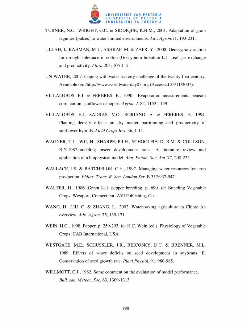
198

TURNER, N.C., WRIGHT, G.C. & SIDDIQUE, K.H.M., 2001. Adaptation of grain

legumes (pulses) to water-limited environments. Adv. Agron.71, 193-231.

ULLAH, I., RAHMAN, M-U, ASHRAF, M. & ZAFR, Y., 2008. Genotypic variation

for drought tolerance in cotton (Gossypium hirsutum L.): Leaf gas exchange

and productivity. Flora 203, 105-115.

UN-WATER, 2007. Coping with water scarcity-challenge of the twenty-first century.

Available on: /http://www.worldwaterday07.org (Accessed 23/11/2007).

VILLALOBOS, F.J. & FERERES, E., 1990. Evaporation measurements beneath

corn, cotton, sunflower canopies. Agron. J. 82, 1153-1159.

VILLALOBOS, F.J., SADRAS, V.O., SORIANO, A. & FERERES, E., 1994.

Planting density effects on dry matter partitioning and productivity of

sunflower hybrids. Field Crops Res. 36, 1-11.

WAGNER, T.L., WU, H., SHARPE, P.J.H., SCHOOLFIELD, R.M. & COULSON,

R.N.1987.modeling insect development rates: A literature review and

application of a biophysical model. Ann. Entom. Soc. Am. 77, 208-225.

WALLACE, J.S. & BATCHELOR, C.H., 1997. Managing water resources for crop

production. Philos. Trans. R. Soc. London Ser. B 352:937-947.

WALTER, H., 1986. Green leaf. pepper breeding. p. 690. In: Breeding Vegetable

Crops. Westport, Connecticut: AVI Publishing, Co.

WANG, H., LIU, C. & ZHANG, L., 2002. Water-saving agriculture in China: An

overview. Adv. Agron. 75, 135-171.

WEIN, H.C., 1998. Pepper. p. 259-293. In: H.C. Wein (ed.). Physiology of Vegetable

Crops. CAB International, USA.

WESTGATE, M.E., SCHUSSLER, J.R., REICOSKY, D.C. & BRENNER, M.L.

1989. Effects of water deficits on seed development in soybeans. II.

Conservation of seed growth rate. Plant Physiol. 91, 980-985.

WILLMOTT, C.J., 1982. Some comment on the evaluation of model performance.

Bull. Am. Meteor. Soc. 63, 1309-1313.

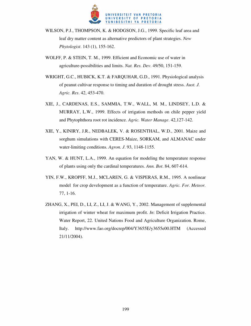
199

WILSON, P.J., THOMPSON, K. & HODGSON, J.G., 1999. Specific leaf area and

leaf dry matter content as alternative predictors of plant strategies. New

Phytologist. 143 (1), 155-162.

WOLFF, P. & STEIN, T. M., 1999. Efficient and Economic use of water in

agriculture-possibilities and limits. Nat. Res. Dev. 49/50, 151-159.

WRIGHT, G.C., HUBICK, K.T. & FARQUHAR, G.D., 1991. Physiological analysis

of peanut cultivar response to timing and duration of drought stress. Aust. J.

Agric. Res. 42, 453-470.

XIE, J., CARDENAS, E.S., SAMMIA, T.W., WALL, M. M., LINDSEY, L.D. &

MURRAY, L.W., 1999. Effects of irrigation methods on chile pepper yield

and Phytophthora root rot incidence. Agric. Water Manage. 42,127-142.

XIE, Y., KINIRY, J.R., NEDBALEK, V. & ROSENTHAL, W.D., 2001. Maize and

sorghum simulations with CERES-Maize, SORKAM, and ALMANAC under

water-limiting conditions. Agron. J. 93, 1148-1155.

YAN, W. & HUNT, L.A., 1999. An equation for modeling the temperature response

of plants using only the cardinal temperatures. Ann. Bot. 84, 607-614.

YIN, F.W., KROPFF, M.J., MCLAREN, G. & VISPERAS, R.M., 1995. A nonlinear

model for crop development as a function of temperature. Agric. For. Meteor.

77, 1-16.

ZHANG, X., PEI, D., LI, Z., LI, J. & WANG, Y., 2002. Management of supplemental

irrigation of winter wheat for maximum profit. In: Deficit Irrigation Practice.

Water Report, 22. United Nations Food and Agriculture Organization. Rome,

Italy. http://www.fao.org/docrep/004/Y3655E/y3655e00.HTM (Accessed

21/11/2004).

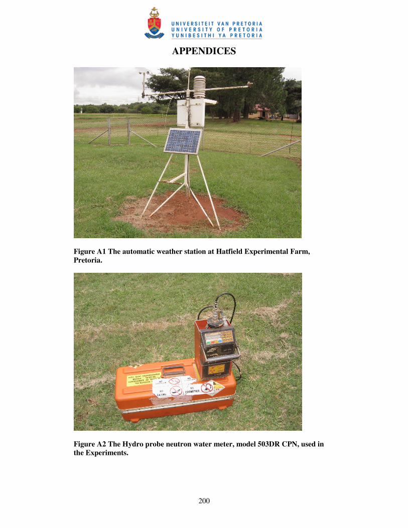
200

APPENDICES

Figure A1 The automatic weather station at Hatfield Experimental Farm, Pretoria.

Figure A2 The Hydro probe neutron water meter, model 503DR CPN, used in the Experiments.

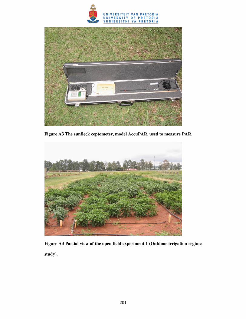
201

Figure A3 The sunfleck ceptometer, model AccuPAR, used to measure PAR.

Figure A3 Partial view of the open field experiment 1 (Outdoor irrigation regime

study).

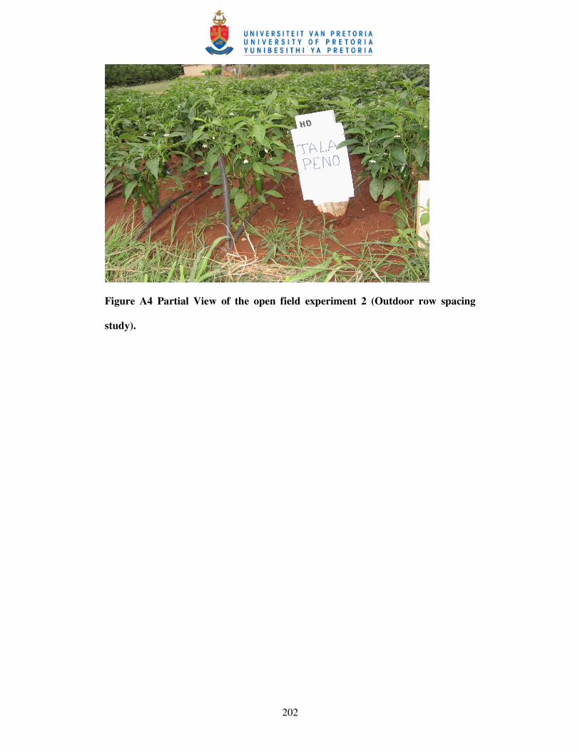
202

Figure A4 Partial View of the open field experiment 2 (Outdoor row spacing

study).

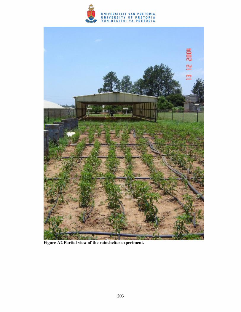
203

Figure A2 Partial view of the rainshelter experiment.

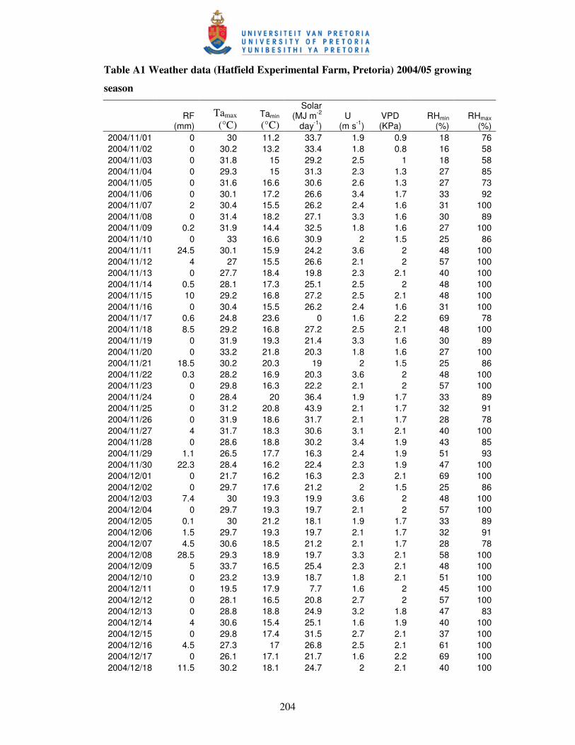
204

Table A1 Weather data (Hatfield Experimental Farm, Pretoria) 2004/05 growing

season

RF

(mm) Tamax

(°C) Tamin (°C)

Solar (MJ m-2

day-1) U

(m s-1) VPD (KPa)

RHmin (%)

RHmax (%)

2004/11/01 0 30 11.2 33.7 1.9 0.9 18 76 2004/11/02 0 30.2 13.2 33.4 1.8 0.8 16 58 2004/11/03 0 31.8 15 29.2 2.5 1 18 58 2004/11/04 0 29.3 15 31.3 2.3 1.3 27 85 2004/11/05 0 31.6 16.6 30.6 2.6 1.3 27 73 2004/11/06 0 30.1 17.2 26.6 3.4 1.7 33 92 2004/11/07 2 30.4 15.5 26.2 2.4 1.6 31 100 2004/11/08 0 31.4 18.2 27.1 3.3 1.6 30 89 2004/11/09 0.2 31.9 14.4 32.5 1.8 1.6 27 100 2004/11/10 0 33 16.6 30.9 2 1.5 25 86 2004/11/11 24.5 30.1 15.9 24.2 3.6 2 48 100 2004/11/12 4 27 15.5 26.6 2.1 2 57 100 2004/11/13 0 27.7 18.4 19.8 2.3 2.1 40 100 2004/11/14 0.5 28.1 17.3 25.1 2.5 2 48 100 2004/11/15 10 29.2 16.8 27.2 2.5 2.1 48 100 2004/11/16 0 30.4 15.5 26.2 2.4 1.6 31 100 2004/11/17 0.6 24.8 23.6 0 1.6 2.2 69 78 2004/11/18 8.5 29.2 16.8 27.2 2.5 2.1 48 100 2004/11/19 0 31.9 19.3 21.4 3.3 1.6 30 89 2004/11/20 0 33.2 21.8 20.3 1.8 1.6 27 100 2004/11/21 18.5 30.2 20.3 19 2 1.5 25 86 2004/11/22 0.3 28.2 16.9 20.3 3.6 2 48 100 2004/11/23 0 29.8 16.3 22.2 2.1 2 57 100 2004/11/24 0 28.4 20 36.4 1.9 1.7 33 89 2004/11/25 0 31.2 20.8 43.9 2.1 1.7 32 91 2004/11/26 0 31.9 18.6 31.7 2.1 1.7 28 78 2004/11/27 4 31.7 18.3 30.6 3.1 2.1 40 100 2004/11/28 0 28.6 18.8 30.2 3.4 1.9 43 85 2004/11/29 1.1 26.5 17.7 16.3 2.4 1.9 51 93 2004/11/30 22.3 28.4 16.2 22.4 2.3 1.9 47 100 2004/12/01 0 21.7 16.2 16.3 2.3 2.1 69 100 2004/12/02 0 29.7 17.6 21.2 2 1.5 25 86 2004/12/03 7.4 30 19.3 19.9 3.6 2 48 100 2004/12/04 0 29.7 19.3 19.7 2.1 2 57 100 2004/12/05 0.1 30 21.2 18.1 1.9 1.7 33 89 2004/12/06 1.5 29.7 19.3 19.7 2.1 1.7 32 91 2004/12/07 4.5 30.6 18.5 21.2 2.1 1.7 28 78 2004/12/08 28.5 29.3 18.9 19.7 3.3 2.1 58 100 2004/12/09 5 33.7 16.5 25.4 2.3 2.1 48 100 2004/12/10 0 23.2 13.9 18.7 1.8 2.1 51 100 2004/12/11 0 19.5 17.9 7.7 1.6 2 45 100 2004/12/12 0 28.1 16.5 20.8 2.7 2 57 100 2004/12/13 0 28.8 18.8 24.9 3.2 1.8 47 83 2004/12/14 4 30.6 15.4 25.1 1.6 1.9 40 100 2004/12/15 0 29.8 17.4 31.5 2.7 2.1 37 100 2004/12/16 4.5 27.3 17 26.8 2.5 2.1 61 100 2004/12/17 0 26.1 17.1 21.7 1.6 2.2 69 100 2004/12/18 11.5 30.2 18.1 24.7 2 2.1 40 100

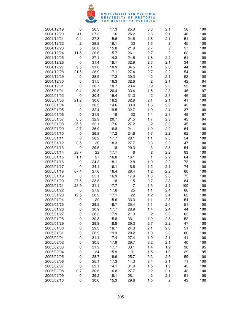
205

2004/12/19 0 26.5 17.3 25.3 3.3 2.1 58 100 2004/12/20 41 27.3 16 25.2 2.3 2.1 48 100 2004/12/21 0.4 27.3 15.6 24.6 1.8 2.1 51 100 2004/12/22 2 28.9 16.1 33 1.6 2 45 100 2004/12/23 5 26.8 15.8 21.9 2.7 2 57 100 2004/12/24 11.5 26.6 15.7 26.1 2.7 2 62 100 2004/12/25 0 27.1 14.3 24.6 1.8 2.2 61 100 2004/12/26 0 31.4 18.1 32.9 2.3 2.1 34 100 2004/12/27 9.5 31.6 18.9 34.5 2.1 2.3 44 100 2004/12/28 21.5 28.9 17.1 27.4 2.7 2.2 54 100 2004/12/29 0 28.9 17.2 30.3 2 2.1 52 100 2004/12/30 0 31.5 18.3 32.6 2 2.1 42 94 2004/12/31 0 30.7 18.7 23.4 0.9 2.3 53 100 2005/01/01 0.4 30.8 20.4 33.4 1.5 2.3 46 97 2005/01/02 0 30.4 19.4 31.3 2 2.3 46 100 2005/01/03 21.2 30.6 18.2 32.9 2.1 2.1 41 100 2005/01/04 0 30.5 14.6 33.9 1.6 2.2 43 100 2005/01/05 0 32.4 19.5 32.7 1.9 2.4 37 100 2005/01/06 0 31.9 18 32 1.4 2.3 48 97 2005/01/07 0.5 32.9 20.7 31.5 1.7 2.3 43 94 2005/01/08 25.5 32.1 17.6 27.2 2 2.3 45 100 2005/01/09 2.7 26.9 16.8 24.1 1.9 2.2 64 100 2005/01/10 0 26.8 17.2 24.6 1.7 2.2 62 100 2005/01/11 0 28.2 17.7 28.1 1.1 2.3 54 100 2005/01/12 0.5 30 18.3 27.7 3.3 2.2 47 100 2005/01/13 0 29.5 18 29.3 3 2.3 54 100 2005/01/14 29.7 22 17.1 6 2 2.2 93 100 2005/01/15 1.1 27 16.8 16.1 1 2.2 64 100 2005/01/16 0 24.3 18.1 12.8 1.9 2.2 73 100 2005/01/17 0 24.1 16.1 16.6 1.2 2.1 74 100 2005/01/18 67.4 27.6 16.4 26.4 1.2 2.2 60 100 2005/01/19 0 25.1 16.9 17.9 1.3 2.3 75 100 2005/01/20 27.5 23.8 18 11.5 0.7 2.3 84 100 2005/01/21 28.9 21.1 17.7 7 1.3 2.2 100 100 2005/01/22 0 27.8 17.6 25 1.1 2.4 66 100 2005/01/23 12.5 28.9 17.1 22 1.2 2.4 62 100 2005/01/24 0 29 15.6 33.3 1.1 2.3 54 100 2005/01/25 0 29.5 18.7 25.4 1.1 2.4 51 100 2005/01/26 0 30.9 17.7 28.9 1.4 2.4 44 100 2005/01/27 0 28.2 17.9 21.9 2 2.3 63 100 2005/01/28 0 30.3 15.8 33.1 1.9 2.3 52 100 2005/01/29 0 29.8 18.8 29.3 2.7 2.2 47 100 2005/01/30 0 29.3 18.7 24.3 2.1 2.3 51 100 2005/01/31 0 26.9 19.3 20.2 1.9 2.3 60 100 2005/02/01 0 31.1 17.4 27.4 1.9 2.1 41 100 2005/02/02 0 30.5 17.9 29.7 2.2 2.1 40 100 2005/02/03 0 31.9 17.7 33.1 1.4 1.9 30 95 2005/02/04 0 34 15.9 31 1.5 1.9 29 95 2005/02/05 0 28.7 18.6 25.7 3.3 2.3 59 100 2005/02/06 0 25.1 17.3 14.3 2.4 2.1 71 100 2005/02/07 0 29.1 14.1 31.9 1.5 1.9 43 100 2005/02/08 0.7 30.6 16.8 27.7 2.2 2.1 42 100 2005/02/09 0 29.2 18.1 28.1 2 2.1 51 100 2005/02/10 0 30.6 15.3 29.6 1.5 2 43 100

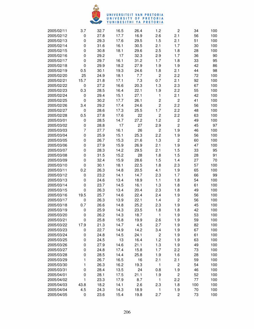
206

2005/02/11 3.7 32.7 16.5 26.4 1.2 2 34 100 2005/02/12 0 27.8 17.7 16.9 2.6 2.1 56 100 2005/02/13 0 29.3 17.6 29.5 1.5 2.1 51 100 2005/02/14 0 31.6 16.1 30.5 2.1 1.7 30 100 2005/02/15 0 30.8 18.1 29.6 2.5 1.8 28 100 2005/02/16 0 29.2 17 32.3 2.9 1.7 36 90 2005/02/17 0 29.7 16.1 31.2 1.7 1.8 33 95 2005/02/18 0 29.9 18.2 27.9 1.9 1.9 42 86 2005/02/19 0.5 30.1 19.3 24.6 1.8 2.1 44 98 2005/02/20 25 24.9 18.1 7.7 2 2.2 72 100 2005/02/21 15.7 21.8 17.1 7.3 0.7 2.1 92 100 2005/02/22 0 27.2 16.6 20.3 1.3 2.3 67 100 2005/02/23 0.3 28.5 16.4 22.1 1.9 2.2 55 100 2005/02/24 0 29.4 15.1 27.1 1 2.1 42 100 2005/02/25 0 30.2 17.7 26.1 2 2 41 100 2005/02/26 3.4 29.2 17.4 24.6 2 2.2 56 100 2005/02/27 0 28.6 17.3 25.5 1.7 2.2 48 100 2005/02/28 0.5 27.8 17.6 22 2 2.2 63 100 2005/03/01 0 28.5 14.7 27.2 1.2 2 49 100 2005/03/02 0 28.8 17 27 2.9 2 45 97 2005/03/03 7 27.7 16.1 26 2 1.9 46 100 2005/03/04 0 25.9 15.1 25.3 2.2 1.9 56 100 2005/03/05 0 26.7 15.3 21.6 1.3 2 60 100 2005/03/06 0 27.9 15.9 26.9 2.1 1.9 47 100 2005/03/07 0 28.3 14.2 29.5 2.1 1.5 33 95 2005/03/08 0 31.5 15.2 28 1.8 1.5 28 91 2005/03/09 0 32.4 15.9 28.6 1.5 1.4 27 70 2005/03/10 0 30.1 18.1 22.5 1.8 2.3 57 100 2005/03/11 0.2 26.3 14.8 20.5 4.1 1.9 65 100 2005/03/12 0 23.2 14.1 14.7 2.3 1.7 66 99 2005/03/13 0 24.6 13.4 18.9 1.1 1.8 54 100 2005/03/14 0 23.7 14.5 16.1 1.3 1.8 61 100 2005/03/15 0 26.3 13.4 20.4 2.3 1.8 49 100 2005/03/16 19.5 25.7 14.6 22.4 2.4 1.9 56 100 2005/03/17 0 26.3 13.9 22.1 1.4 2 56 100 2005/03/18 0.7 26.6 14.8 25.2 2.3 1.9 45 100 2005/03/19 0 25.9 14.3 23.5 1.8 1.8 42 100 2005/03/20 0 26.2 14.3 18.7 1 1.9 53 100 2005/03/21 0 25.8 15.8 19.9 2.6 1.9 59 100 2005/03/22 17.9 21.3 14.7 4.5 2.7 1.9 82 100 2005/03/23 0 22.7 14.9 14.2 3.4 1.9 67 100 2005/03/24 0 24.8 14.5 24.1 2 1.9 61 100 2005/03/25 0 24.5 13 16.4 1.2 1.9 63 100 2005/03/26 0 27.9 14.6 21.1 1.3 1.9 49 100 2005/03/27 0 24.8 17.4 15.8 1.7 2.2 73 100 2005/03/28 0 28.5 14.4 25.8 1.9 1.6 28 100 2005/03/29 1 26.7 16.5 16 2.1 2.1 59 100 2005/03/30 1 26.3 16.2 19.3 1 2 54 100 2005/03/31 0 28.4 13.5 24 0.8 1.9 46 100 2005/04/01 0 28.1 17.5 21.1 1.9 2 52 100 2005/04/02 1 23.3 17.9 8.7 1 2.2 77 100 2005/04/03 43.8 18.2 14.1 2.6 2.3 1.8 100 100 2005/04/04 4.5 24.3 14.3 18.9 1 1.9 70 100 2005/04/05 0 23.6 15.4 19.8 2.7 2 73 100

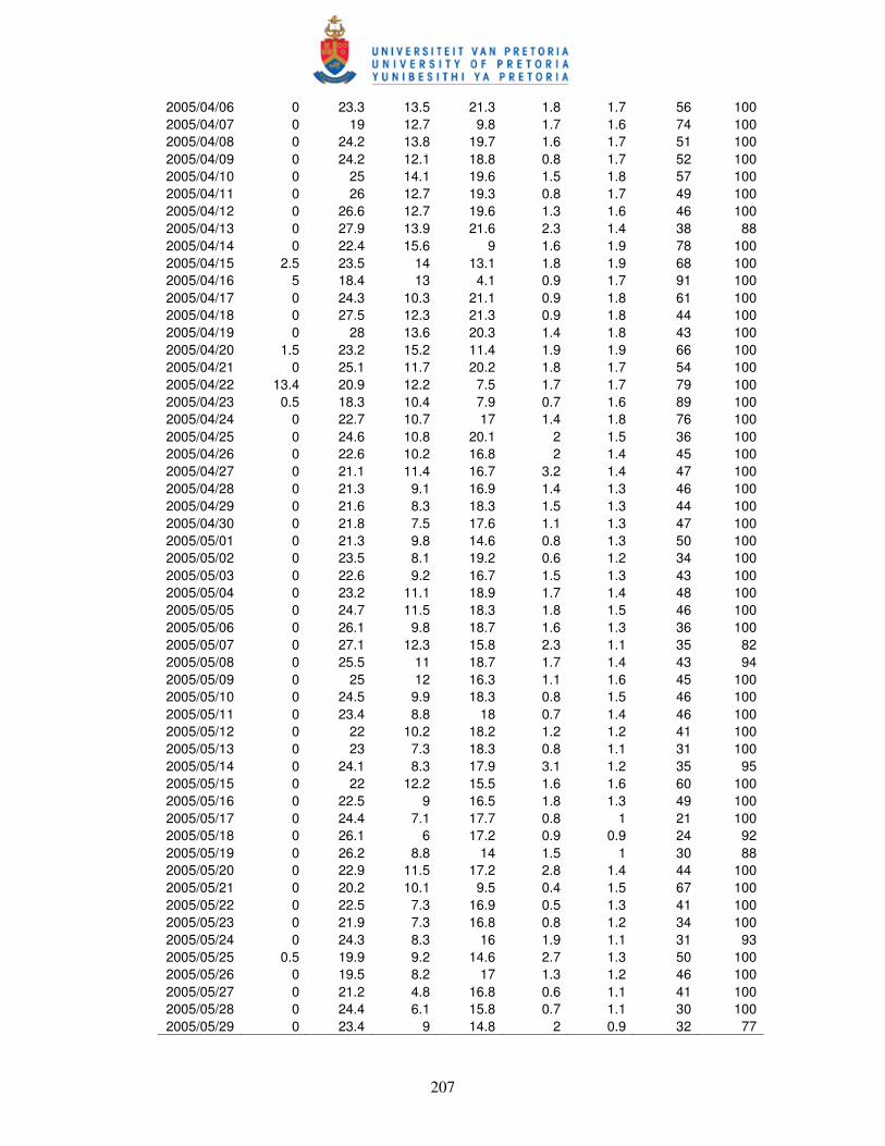
207

2005/04/06 0 23.3 13.5 21.3 1.8 1.7 56 100 2005/04/07 0 19 12.7 9.8 1.7 1.6 74 100 2005/04/08 0 24.2 13.8 19.7 1.6 1.7 51 100 2005/04/09 0 24.2 12.1 18.8 0.8 1.7 52 100 2005/04/10 0 25 14.1 19.6 1.5 1.8 57 100 2005/04/11 0 26 12.7 19.3 0.8 1.7 49 100 2005/04/12 0 26.6 12.7 19.6 1.3 1.6 46 100 2005/04/13 0 27.9 13.9 21.6 2.3 1.4 38 88 2005/04/14 0 22.4 15.6 9 1.6 1.9 78 100 2005/04/15 2.5 23.5 14 13.1 1.8 1.9 68 100 2005/04/16 5 18.4 13 4.1 0.9 1.7 91 100 2005/04/17 0 24.3 10.3 21.1 0.9 1.8 61 100 2005/04/18 0 27.5 12.3 21.3 0.9 1.8 44 100 2005/04/19 0 28 13.6 20.3 1.4 1.8 43 100 2005/04/20 1.5 23.2 15.2 11.4 1.9 1.9 66 100 2005/04/21 0 25.1 11.7 20.2 1.8 1.7 54 100 2005/04/22 13.4 20.9 12.2 7.5 1.7 1.7 79 100 2005/04/23 0.5 18.3 10.4 7.9 0.7 1.6 89 100 2005/04/24 0 22.7 10.7 17 1.4 1.8 76 100 2005/04/25 0 24.6 10.8 20.1 2 1.5 36 100 2005/04/26 0 22.6 10.2 16.8 2 1.4 45 100 2005/04/27 0 21.1 11.4 16.7 3.2 1.4 47 100 2005/04/28 0 21.3 9.1 16.9 1.4 1.3 46 100 2005/04/29 0 21.6 8.3 18.3 1.5 1.3 44 100 2005/04/30 0 21.8 7.5 17.6 1.1 1.3 47 100 2005/05/01 0 21.3 9.8 14.6 0.8 1.3 50 100 2005/05/02 0 23.5 8.1 19.2 0.6 1.2 34 100 2005/05/03 0 22.6 9.2 16.7 1.5 1.3 43 100 2005/05/04 0 23.2 11.1 18.9 1.7 1.4 48 100 2005/05/05 0 24.7 11.5 18.3 1.8 1.5 46 100 2005/05/06 0 26.1 9.8 18.7 1.6 1.3 36 100 2005/05/07 0 27.1 12.3 15.8 2.3 1.1 35 82 2005/05/08 0 25.5 11 18.7 1.7 1.4 43 94 2005/05/09 0 25 12 16.3 1.1 1.6 45 100 2005/05/10 0 24.5 9.9 18.3 0.8 1.5 46 100 2005/05/11 0 23.4 8.8 18 0.7 1.4 46 100 2005/05/12 0 22 10.2 18.2 1.2 1.2 41 100 2005/05/13 0 23 7.3 18.3 0.8 1.1 31 100 2005/05/14 0 24.1 8.3 17.9 3.1 1.2 35 95 2005/05/15 0 22 12.2 15.5 1.6 1.6 60 100 2005/05/16 0 22.5 9 16.5 1.8 1.3 49 100 2005/05/17 0 24.4 7.1 17.7 0.8 1 21 100 2005/05/18 0 26.1 6 17.2 0.9 0.9 24 92 2005/05/19 0 26.2 8.8 14 1.5 1 30 88 2005/05/20 0 22.9 11.5 17.2 2.8 1.4 44 100 2005/05/21 0 20.2 10.1 9.5 0.4 1.5 67 100 2005/05/22 0 22.5 7.3 16.9 0.5 1.3 41 100 2005/05/23 0 21.9 7.3 16.8 0.8 1.2 34 100 2005/05/24 0 24.3 8.3 16 1.9 1.1 31 93 2005/05/25 0.5 19.9 9.2 14.6 2.7 1.3 50 100 2005/05/26 0 19.5 8.2 17 1.3 1.2 46 100 2005/05/27 0 21.2 4.8 16.8 0.6 1.1 41 100 2005/05/28 0 24.4 6.1 15.8 0.7 1.1 30 100 2005/05/29 0 23.4 9 14.8 2 0.9 32 77

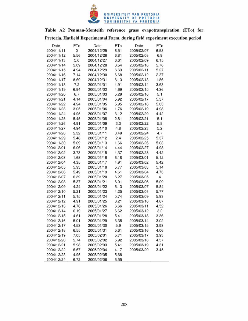
208

Table A2 Penman-Monteith reference grass evapotranspiration (ETo) for

Pretoria, Hatfield Experimental Farm, during field experiment execution period

Date ETo Date ETo Date ETo 2004/11/11 0 2004/12/25 6.51 2005/02/07 6.53 2004/11/12 5.56 2004/12/26 6.81 2005/02/08 6.9 2004/11/13 5.6 2004/12/27 6.61 2005/02/09 6.15 2004/11/14 5.09 2004/12/28 6.54 2005/02/10 5.76 2004/11/15 4.94 2004/12/29 6.63 2005/02/11 5.27 2004/11/16 7.14 2004/12/30 6.68 2005/02/12 2.37 2004/11/17 8.69 2004/12/31 6.13 2005/02/13 1.86 2004/11/18 7.2 2005/01/01 4.91 2005/02/14 3.63 2004/11/19 6.94 2005/01/02 4.69 2005/02/15 4.36 2004/11/20 6.7 2005/01/03 5.29 2005/02/16 5.1 2004/11/21 4.14 2005/01/04 5.92 2005/02/17 5.37 2004/11/22 4.94 2005/01/05 5.95 2005/02/18 5.03 2004/11/23 3.05 2005/01/06 1.76 2005/02/19 4.98 2004/11/24 4.95 2005/01/07 3.12 2005/02/20 4.42 2004/11/25 5.45 2005/01/08 2.81 2005/02/21 5.1 2004/11/26 4.91 2005/01/09 3.3 2005/02/22 5.8 2004/11/27 4.94 2005/01/10 4.8 2005/02/23 5.2 2004/11/28 5.32 2005/01/11 3.49 2005/02/24 4.7 2004/11/29 5.48 2005/01/12 2.4 2005/02/25 5.37 2004/11/30 5.09 2005/01/13 1.66 2005/02/26 5.03 2004/12/01 6.06 2005/01/14 4.44 2005/02/27 4.98 2004/12/02 3.73 2005/01/15 4.37 2005/02/28 4.42 2004/12/03 1.68 2005/01/16 6.18 2005/03/01 5.12 2004/12/04 4.35 2005/01/17 4.91 2005/03/02 5.42 2004/12/05 5.93 2005/01/18 5.77 2005/03/03 5.14 2004/12/06 5.49 2005/01/19 4.61 2005/03/04 4.73 2004/12/07 6.39 2005/01/20 6.27 2005/03/05 4 2004/12/08 5.37 2005/01/21 6.01 2005/03/06 5.09 2004/12/09 4.24 2005/01/22 5.13 2005/03/07 5.84 2004/12/10 5.21 2005/01/23 4.25 2005/03/08 5.77 2004/12/11 5.15 2005/01/24 5.74 2005/03/09 5.93 2004/12/12 4.91 2005/01/25 6.21 2005/03/10 4.67 2004/12/13 4.76 2005/01/26 6.66 2005/03/11 4.52 2004/12/14 6.19 2005/01/27 6.62 2005/03/12 3.2 2004/12/15 4.61 2005/01/28 5.41 2005/03/13 3.36 2004/12/16 5.01 2005/01/29 3.35 2005/03/14 3.02 2004/12/17 4.53 2005/01/30 5.9 2005/03/15 3.93 2004/12/18 6.55 2005/01/31 5.61 2005/03/16 4.06 2004/12/19 7.05 2005/02/01 5.71 2005/03/17 3.93 2004/12/20 5.74 2005/02/02 5.92 2005/03/18 4.57 2004/12/21 5.98 2005/02/03 5.41 2005/03/19 4.31 2004/12/22 6.67 2005/02/04 4.17 2005/03/20 3.45 2004/12/23 4.95 2005/02/05 5.68 2004/12/24 6.72 2005/02/06 6.55

managing the soil water balance of hot pepper (capsicum annuum

Documents