liquid mixing in agitated vessels - · pdf fileliquid mixing in agitated vessels ... the role...
TRANSCRIPT
MULTIPLE IMPELLER GAS-LIQUID CONTACTORS100
5Liquid Mixing in Agitated Vessels
To express the degree of mixing in a stirred vessel, an expression is desirable to show
how far the state of mixing deviates from the ideal complete mixing. The most simple and
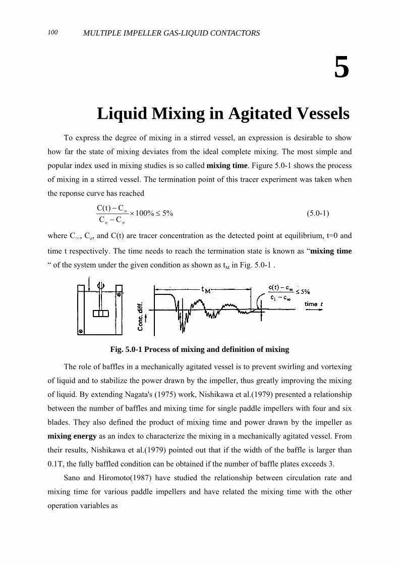
popular index used in mixing studies is so called mixing time. Figure 5.0-1 shows the process
of mixing in a stirred vessel. The termination point of this tracer experiment was taken when
the reponse curve has reached
%5%100CCC)t(C
o
≤×−−
∞
∞ (5.0-1)
where C∞, Co, and C(t) are tracer concentration as the detected point at equilibrium, t=0 and
time t respectively. The time needs to reach the termination state is known as “mixing time
“ of the system under the given condition as shown as tM in Fig. 5.0-1 .
Fig. 5.0-1 Process of mixing and definition of mixing
The role of baffles in a mechanically agitated vessel is to prevent swirling and vortexing
of liquid and to stabilize the power drawn by the impeller, thus greatly improving the mixing
of liquid. By extending Nagata's (1975) work, Nishikawa et al.(1979) presented a relationship
between the number of baffles and mixing time for single paddle impellers with four and six
blades. They also defined the product of mixing time and power drawn by the impeller as
mixing energy as an index to characterize the mixing in a mechanically agitated vessel. From
their results, Nishikawa et al.(1979) pointed out that if the width of the baffle is larger than
0.1T, the fully baffled condition can be obtained if the number of baffle plates exceeds 3.
Sano and Hiromoto(1987) have studied the relationship between circulation rate and
mixing time for various paddle impellers and have related the mixing time with the other
operation variables as
Liquid Mixing in Agitated Vessels 101
NtM=(NtM)F.B./(l-0.62e-6.8α) (5.0-2)
where α=nbB/T and (NtM)F.B.C=2.3(D/T)-1.67(w/T)-0.74nP-0.47
Pandit and Joshi(1982), extending the model proposed by Joshi et al(1982) estimated the
mixing time of the gassed stirred tank and obtained the following equation to predict mixing
time in a gaased agitatated vessel.
15/13/2
4212/1S6/13
M )gWV
DN()NVQ
)(DW()
DT)(
TTaH(41.20Nt +
= (5.0-3)
where the constant "a" depended on the size of the circulation loop and was equal to 1 for a
centrally located impeller.
Nagase and Hiroo(1983) used the conductivity method to investigate the effect of
gassing on the mixing efficiency of the mixing vessels with single vaned disc turbine and disc
turbine. They found that under gassing , the mixing rate was reduced by 20% for the disc
turbine and by 30% for the vaned disc turbine at low gas flow rates compared with ungassed
conditions.
In retrospect, it can be seen that little research has been done for the effect of baffle
design on mixing time in the stirred tank with Rushton impeller under gassing condition in the
previous works. In this chapter, a study using both tracer technique and computer fluid
dynamic approach to discuss how the baffle width, baffle number, rotational speed, gassing
rate and impeller number will affect the extent of liquid mixing in a mechanically agitated
vessel with Rushton turbine impeller.
5.1 Determination of Mixing Time for a Given System by Simulation
To determine the mixing time under extreme baffle conditions, several rotational speeds
and the mixing time for multiple impellers systems, a numerical simulation program was
devised to estimate the mixing time of the system with and without gassing. The
commercially available computer software "Fluent" was used to simulate the single phase
flow field of the individual agitated system. During the simulation, the impeller was always
confined in a black box and the boundary conditions were set on the edges of this box. The
boundary conditions including the kinetic energy, radial velocity, tangential velocity and
vertical velocity were set after the LDA (Laser Doppler Anemometer) measurements,
however the energy dissipasion rate was estimated from an expression proposed by Wu and
Patterson (1989) (ε=Aκ3/2/Lres). The κ - ε turbulent model was adopted to determined the
Reynolds stresses. Once the single phase flow field be detennined, the liquid velocity with
gassing can be calculated from the results of Bakker and Van der Akker(1994) as follows:
MULTIPLE IMPELLER GAS-LIQUID CONTACTORS102
Ul,g=Ul,u×(Pg/Po)β (5.1-1)
where Ul,g and Ul,u are the liquid phase velocity with and without gassing, Pg and Po are the
power consumption with and without gassing respectively. Then, the liquid volumetric flow
rate can be calculated as follows:
qi,l,g=Ul,g×(areai,pro)×(1-εg)β (5.1-2)
where qi,l,g was the liquid volumetric flow rate between cells in the i direction, aerai,pro is the
projective area to the t direction and εg is the value of local gas hold-up which are obtained
from the experimental dat of Jian(1992) and Lin(1994). By using the numerical simulation
program, the mixing time of the system under gassed and ungassed conditions can be
estimated and the most suitable exponent "β' was found to be 1 by comparing the simulated
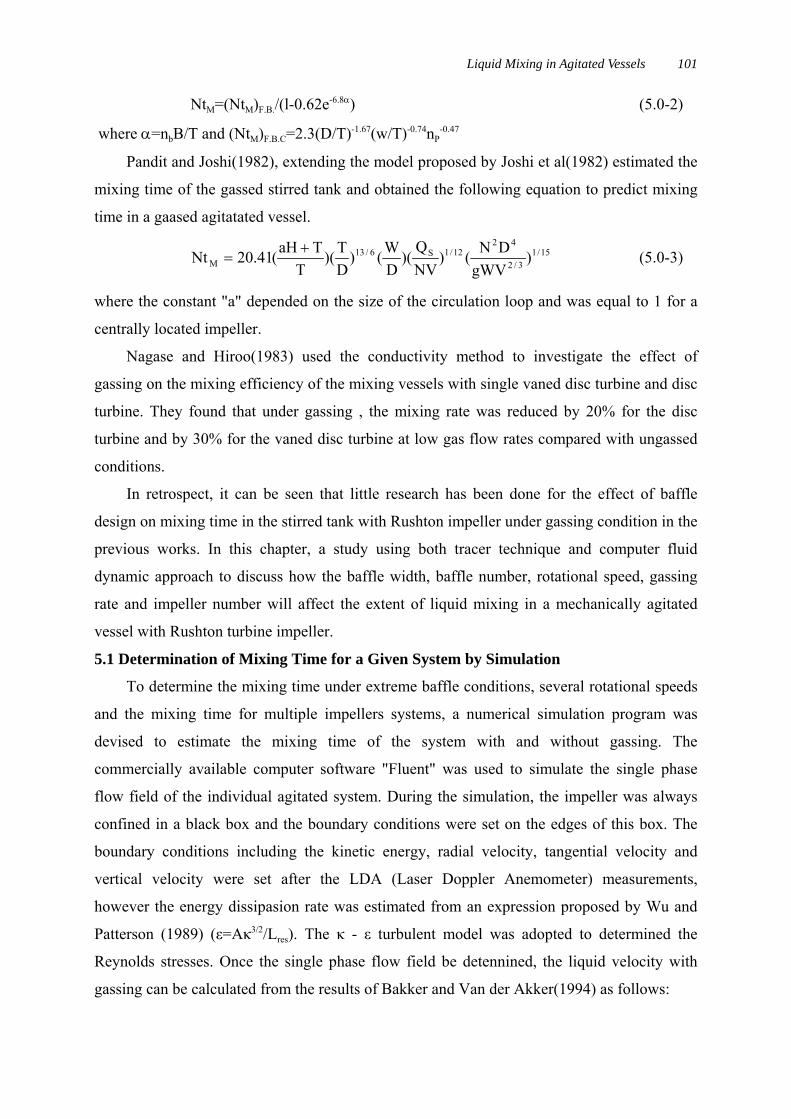
mixing time with the expenmental value.The procedures of this simulation is depicted in
Fig.5.l-1 and the details can be found in Wu's thesis(1996).
Fig. 5.1-1 The flow diagram of the simulated procedure for estimating the mixing timein gas-liquid agitated vessel.
Liquid Mixing in Agitated Vessels 103
Table 5.1-1 compares the simulated results with the experimental data, from which it can
be seen that the simulation results can agree with the experimental data within a range of 10%
deviation under gassed and ungassed conditions.
Table 5.1-1 Comparison of mixing time (tM) between experimental and simulatedmethods.
Baffle Width
Mixing Time0.05T 0.075T 0.1T 0.15T 0.2T
Experimental data (sec) 14.6 13.7 13.0 12.1 11.5simulated data (sec) 14.8 14.2 13.4 12.0 11.7
SingleImpellerSystem
nb=2Qg= 0L/min
deviation (%) 1.30 3.60 3.00 0.83 1.74
5.2 Effect of Baffle Design on Mixing in Single Impeller System without Aeration
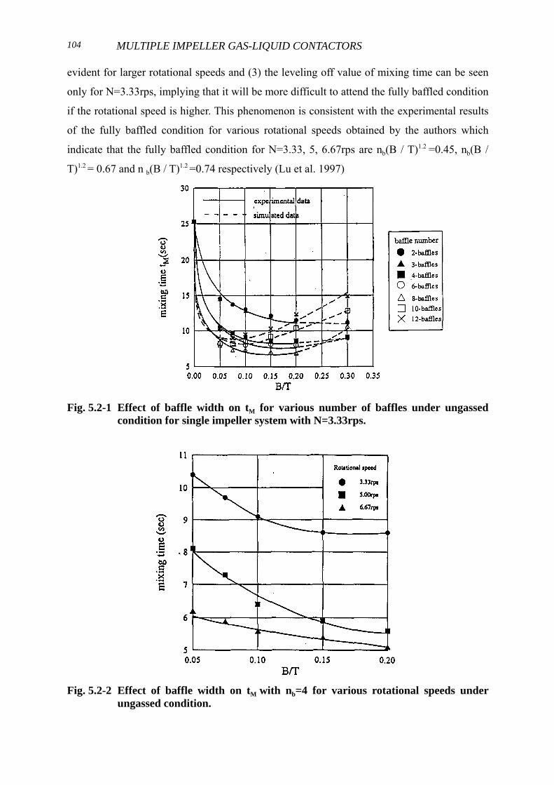
Figure 5.2-1 shows how the width and the number of baffle affect the extent of liquid
mixing of the single impeller system under ungassed conditions for N=3.33rps in term of
"mixing time". The results clearly indicate that insertion of baffles in the system can greatly
improve the liquid mixing even when the ratio of B/T is less than 0.05. However, the fully
baffled condition is difficult to achieve if the baffle number is less than three, which can be
seen from the continuous decay curves for nb= 2 and 3 in this figure. This result is different
from what was observed by Nishikawa et al.(1979) for paddle impeller system which states
that if nb≧2 , the fully baffled condition can be obtained. In the systems for which the baffle
number is more than four, the mixing time decreases steeply with the increase of the width of
the baffle first, then it soon reaches a constant value as B/T exceeds 0.1. It is interesting to
note that this leveling off value tends to decrease as the number of baffles increases in the
range of nb< 8 and B/T< 0.20. This fact implies that within this range, the increase of nb and
B/T will improve the extent of liquid mixing. However. the simulated results as shown in the
figure by dotted lines also point out that the quality of liquid mixing will become worse if nb
is more than eight or B/T is larger than 0.25. The trend of growing worse in mixing is due to
the localizing effect of excessive baffling. If the same plots are drawn for N= 5 and 6.67rps, it
will be found that the trends of mixing tune are very similar to Fig.5.2-1. However the
continuous decay of the mixing time with the increase of baffle width still exists for nb=4 and
the mixing time does not reach a leveling off value until B/T>0.15 and nb≥6. Figure 5.2-2
shows the relationship between the mixing time and baffle width for nb = 4 under various
rotational speeds. It clearly indicates that (1)the increase of rotational speed will increase the
liquid pumping capacity of the impeller thus the mixing quality will be improved;(2) the
continuous decay trend of mixing time with the increase of baffle width becomes more
MULTIPLE IMPELLER GAS-LIQUID CONTACTORS104
evident for larger rotational speeds and (3) the leveling off value of mixing time can be seen
only for N=3.33rps, implying that it will be more difficult to attend the fully baffled condition
if the rotational speed is higher. This phenomenon is consistent with the experimental results
of the fully baffled condition for various rotational speeds obtained by the authors which
indicate that the fully baffled condition for N=3.33, 5, 6.67rps are nb(B / T)1.2 =0.45, nb(B /
T)1.2 = 0.67 and n b(B / T)1.2 =0.74 respectively (Lu et al. 1997)
Fig. 5.2-1 Effect of baffle width on tM for various number of baffles under ungassedcondition for single impeller system with N=3.33rps.
Fig. 5.2-2 Effect of baffle width on tM with nb=4 for various rotational speeds underungassed condition.
Liquid Mixing in Agitated Vessels 105
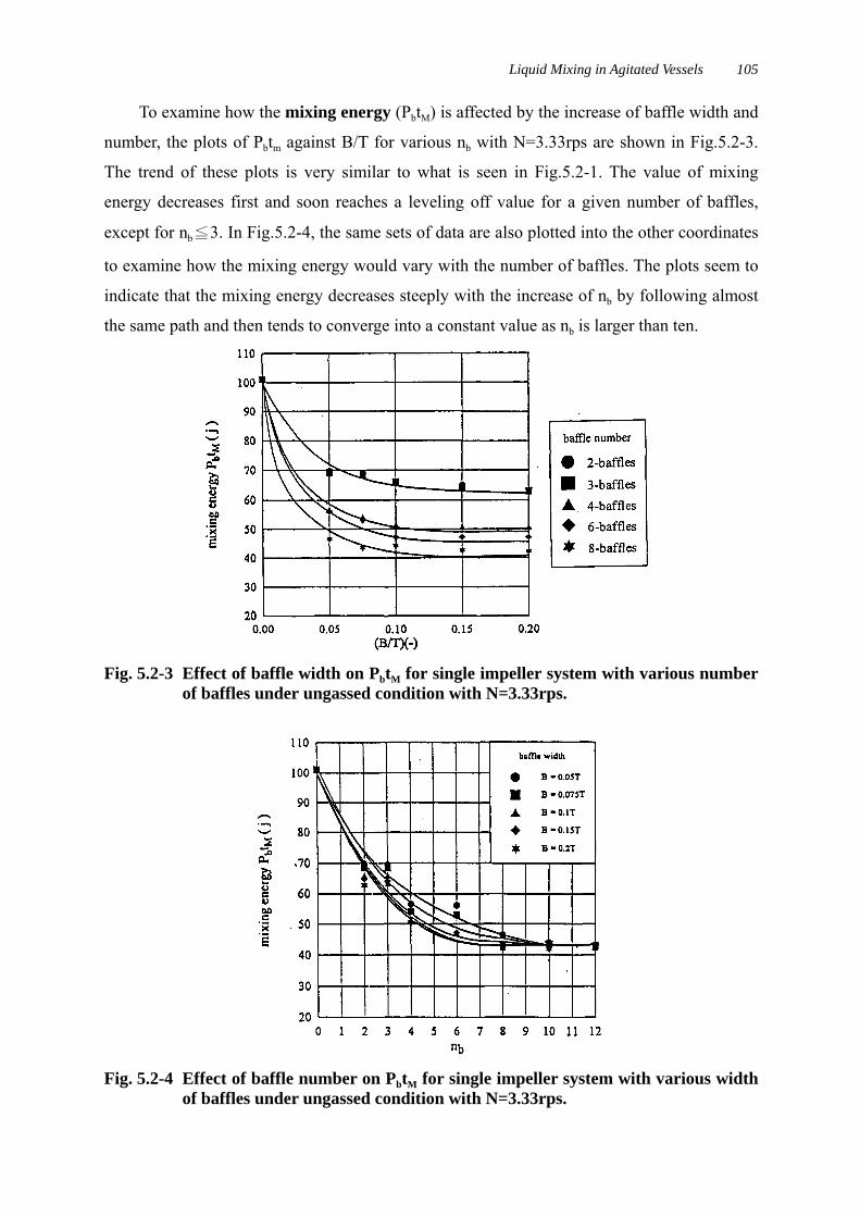
To examine how the mixing energy (PbtM) is affected by the increase of baffle width and
number, the plots of Pbtm against B/T for various nb with N=3.33rps are shown in Fig.5.2-3.
The trend of these plots is very similar to what is seen in Fig.5.2-1. The value of mixing
energy decreases first and soon reaches a leveling off value for a given number of baffles,
except for nb≦3. In Fig.5.2-4, the same sets of data are also plotted into the other coordinates
to examine how the mixing energy would vary with the number of baffles. The plots seem to
indicate that the mixing energy decreases steeply with the increase of nb by following almost
the same path and then tends to converge into a constant value as nb is larger than ten.
Fig. 5.2-3 Effect of baffle width on PbtM for single impeller system with various numberof baffles under ungassed condition with N=3.33rps.
Fig. 5.2-4 Effect of baffle number on PbtM for single impeller system with various widthof baffles under ungassed condition with N=3.33rps.
MULTIPLE IMPELLER GAS-LIQUID CONTACTORS106
5.3 Effect of Baffle Design on Mixing in Single Impeller System with Aeration
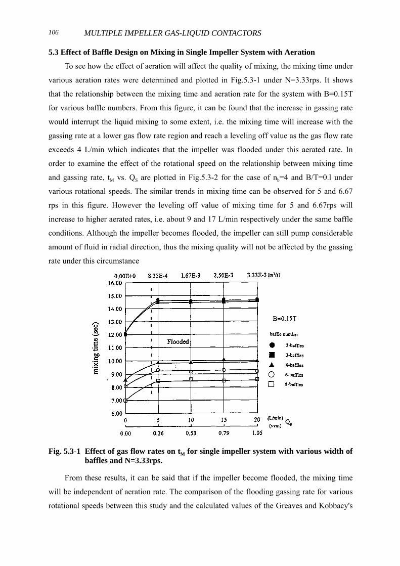
To see how the effect of aeration will affect the quality of mixing, the mixing time under
various aeration rates were determined and plotted in Fig.5.3-1 under N=3.33rps. It shows
that the relationship between the mixing time and aeration rate for the system with B=0.15T
for various baffle numbers. From this figure, it can be found that the increase in gassing rate
would interrupt the liquid mixing to some extent, i.e. the mixing time will increase with the
gassing rate at a lower gas flow rate region and reach a leveling off value as the gas flow rate
exceeds 4 L/min which indicates that the impeller was flooded under this aerated rate. In
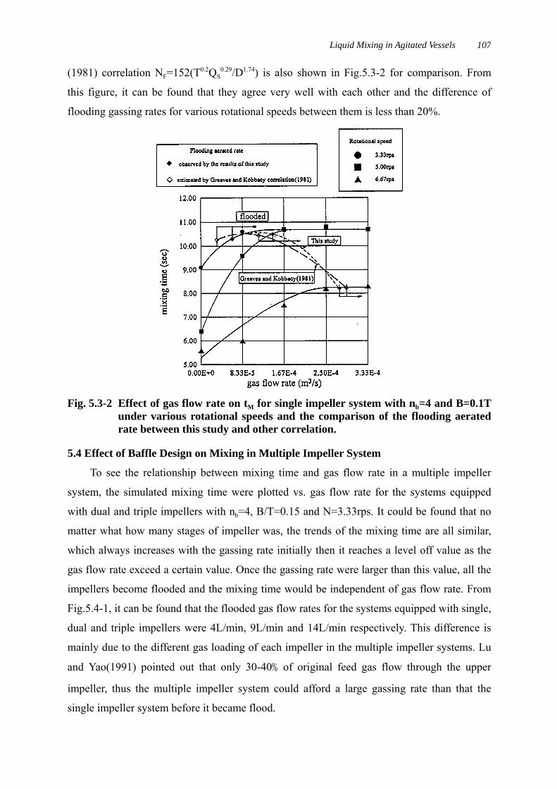
order to examine the effect of the rotational speed on the relationship between mixing time
and gassing rate, tM vs. QS are plotted in Fig.5.3-2 for the case of nb=4 and B/T=0.l under
various rotational speeds. The similar trends in mixing time can be observed for 5 and 6.67
rps in this figure. However the leveling off value of mixing time for 5 and 6.67rps will
increase to higher aerated rates, i.e. about 9 and 17 L/min respectively under the same baffle
conditions. Although the impeller becomes flooded, the impeller can still pump considerable
amount of fluid in radial direction, thus the mixing quality will not be affected by the gassing
rate under this circumstance
Fig. 5.3-1 Effect of gas flow rates on tM for single impeller system with various width ofbaffles and N=3.33rps.
From these results, it can be said that if the impeller become flooded, the mixing time
will be independent of aeration rate. The comparison of the flooding gassing rate for various
rotational speeds between this study and the calculated values of the Greaves and Kobbacy's
Liquid Mixing in Agitated Vessels 107
(1981) correlation NF=152(T0.2QS0.29/D1.74) is also shown in Fig.5.3-2 for comparison. From
this figure, it can be found that they agree very well with each other and the difference of
flooding gassing rates for various rotational speeds between them is less than 20%.
Fig. 5.3-2 Effect of gas flow rate on tM for single impeller system with nb=4 and B=0.1Tunder various rotational speeds and the comparison of the flooding aeratedrate between this study and other correlation.
5.4 Effect of Baffle Design on Mixing in Multiple Impeller System
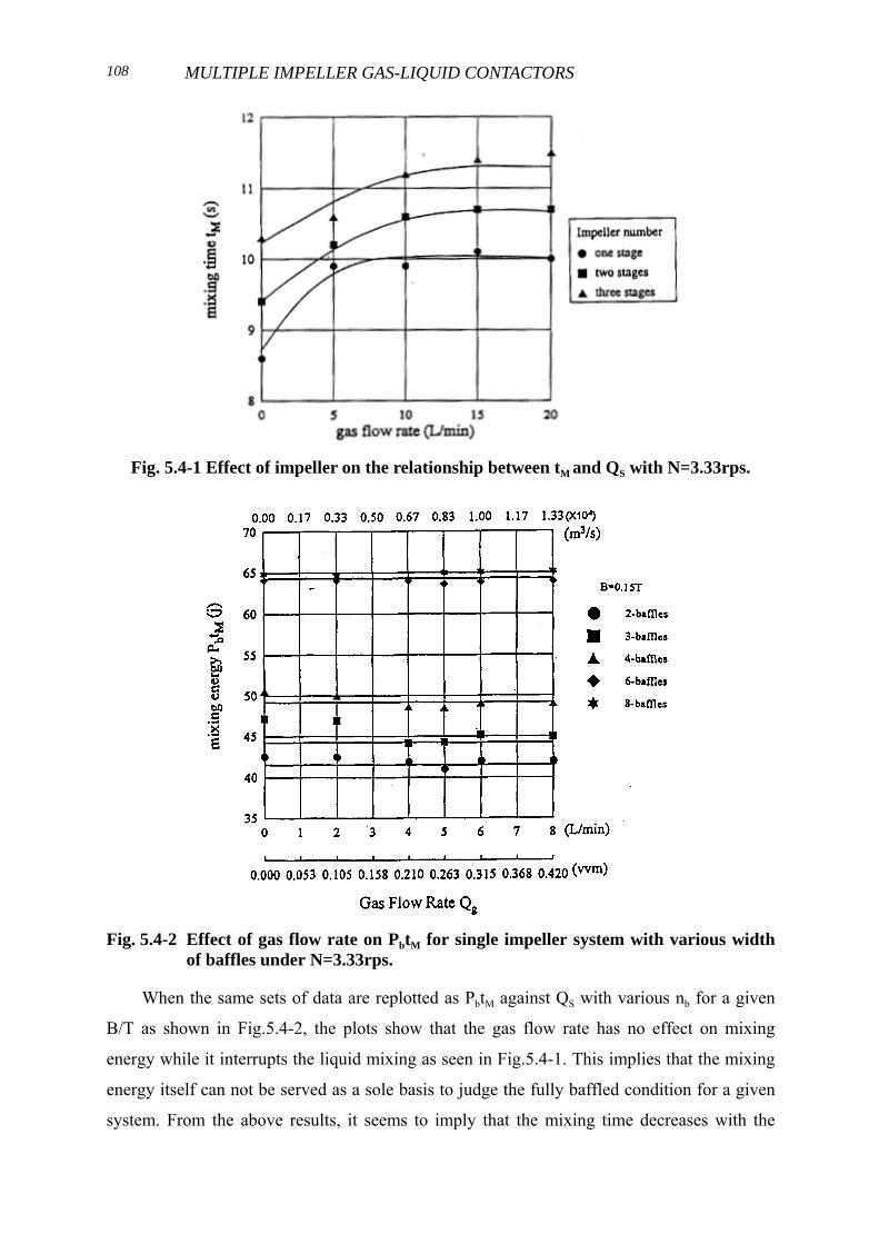
To see the relationship between mixing time and gas flow rate in a multiple impeller
system, the simulated mixing time were plotted vs. gas flow rate for the systems equipped
with dual and triple impellers with nb=4, B/T=0.15 and N=3.33rps. It could be found that no
matter what how many stages of impeller was, the trends of the mixing time are all similar,
which always increases with the gassing rate initially then it reaches a level off value as the
gas flow rate exceed a certain value. Once the gassing rate were larger than this value, all the
impellers become flooded and the mixing time would be independent of gas flow rate. From
Fig.5.4-1, it can be found that the flooded gas flow rates for the systems equipped with single,
dual and triple impellers were 4L/min, 9L/min and 14L/min respectively. This difference is
mainly due to the different gas loading of each impeller in the multiple impeller systems. Lu
and Yao(1991) pointed out that only 30-40﹪of original feed gas flow through the upper
impeller, thus the multiple impeller system could afford a large gassing rate than that the
single impeller system before it became flood.
MULTIPLE IMPELLER GAS-LIQUID CONTACTORS108
Fig. 5.4-1 Effect of impeller on the relationship between tM and QS with N=3.33rps.
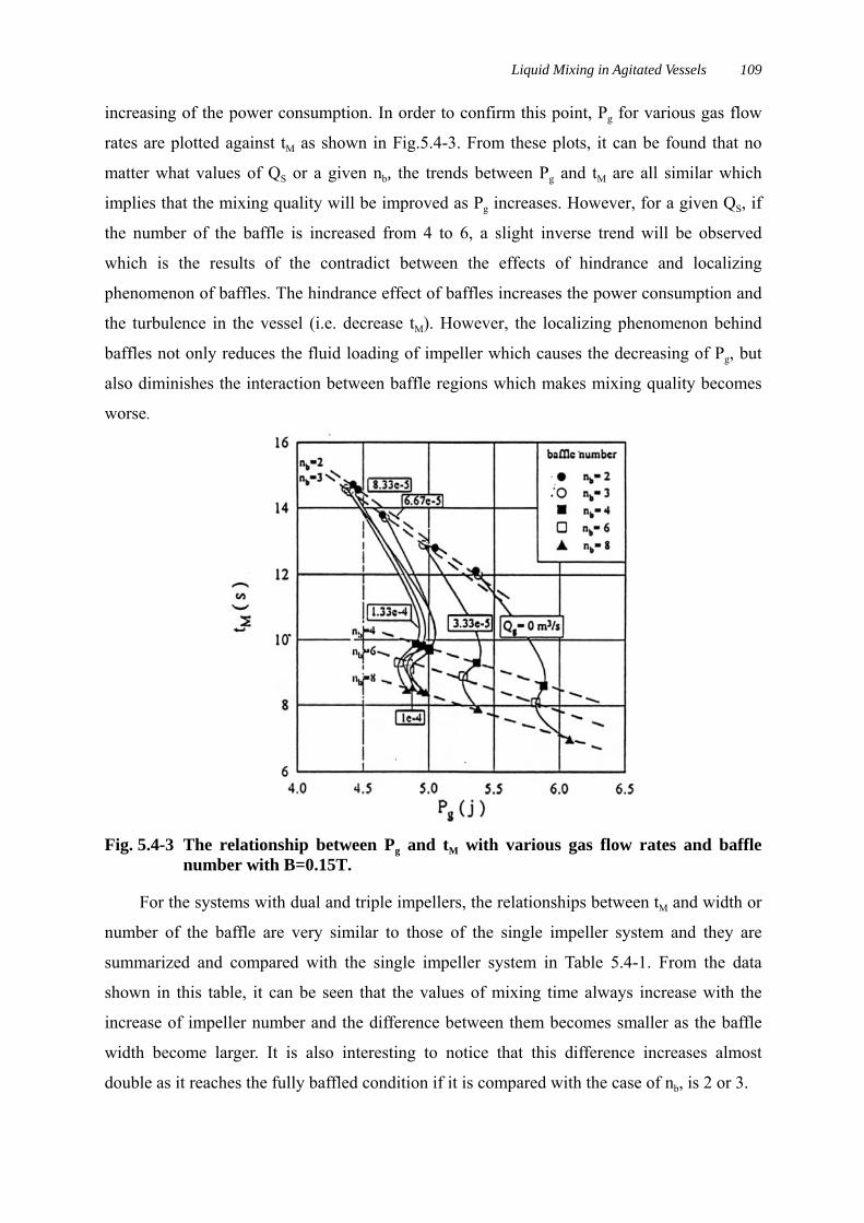
Fig. 5.4-2 Effect of gas flow rate on PbtM for single impeller system with various widthof baffles under N=3.33rps.
When the same sets of data are replotted as PbtM against QS with various nb for a given
B/T as shown in Fig.5.4-2, the plots show that the gas flow rate has no effect on mixing
energy while it interrupts the liquid mixing as seen in Fig.5.4-1. This implies that the mixing
energy itself can not be served as a sole basis to judge the fully baffled condition for a given
system. From the above results, it seems to imply that the mixing time decreases with the
Liquid Mixing in Agitated Vessels 109
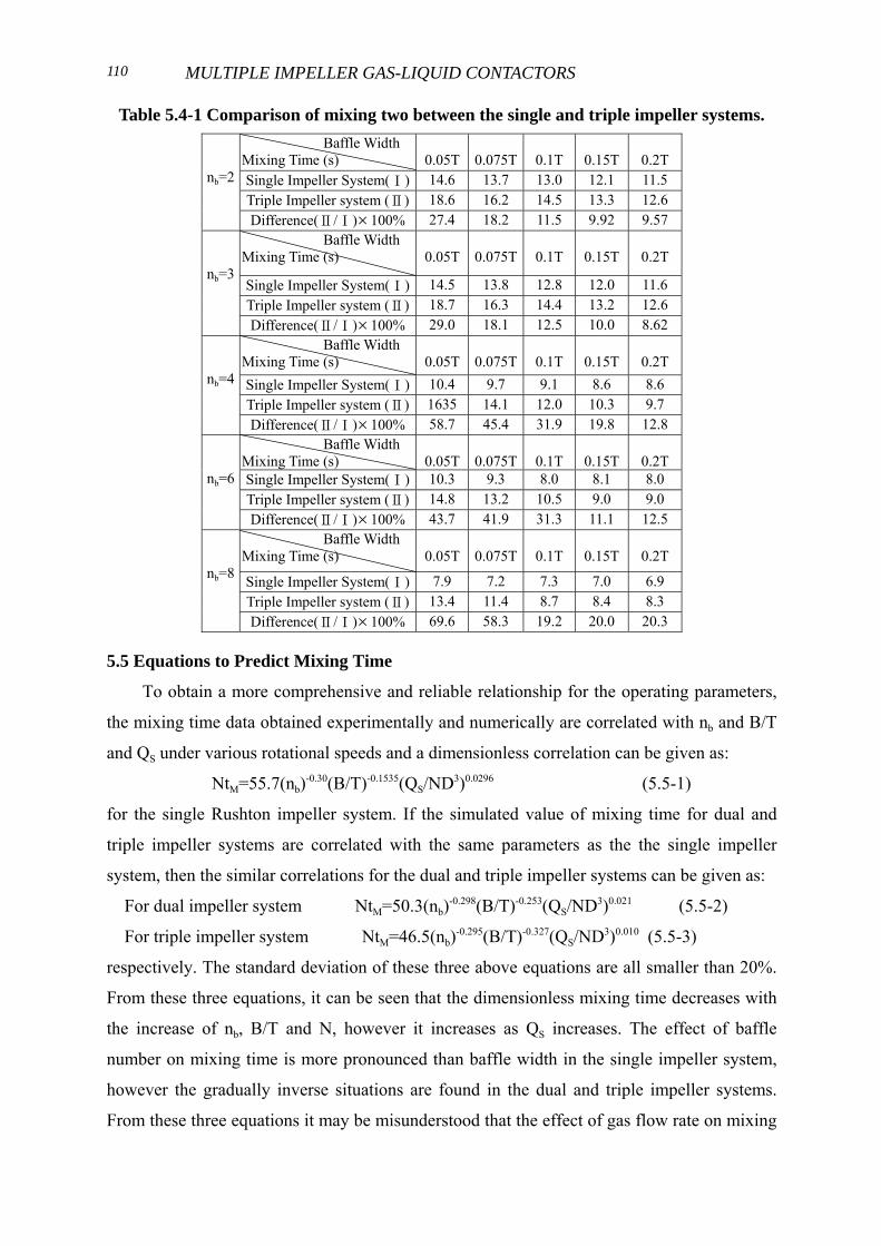
increasing of the power consumption. In order to confirm this point, Pg for various gas flow
rates are plotted against tM as shown in Fig.5.4-3. From these plots, it can be found that no
matter what values of QS or a given nb, the trends between Pg and tM are all similar which
implies that the mixing quality will be improved as Pg increases. However, for a given QS, if
the number of the baffle is increased from 4 to 6, a slight inverse trend will be observed
which is the results of the contradict between the effects of hindrance and localizing
phenomenon of baffles. The hindrance effect of baffles increases the power consumption and
the turbulence in the vessel (i.e. decrease tM). However, the localizing phenomenon behind
baffles not only reduces the fluid loading of impeller which causes the decreasing of Pg, but
also diminishes the interaction between baffle regions which makes mixing quality becomes
worse.
Fig. 5.4-3 The relationship between Pg and tM with various gas flow rates and bafflenumber with B=0.15T.
For the systems with dual and triple impellers, the relationships between tM and width or
number of the baffle are very similar to those of the single impeller system and they are
summarized and compared with the single impeller system in Table 5.4-1. From the data
shown in this table, it can be seen that the values of mixing time always increase with the
increase of impeller number and the difference between them becomes smaller as the baffle
width become larger. It is also interesting to notice that this difference increases almost
double as it reaches the fully baffled condition if it is compared with the case of nb, is 2 or 3.
MULTIPLE IMPELLER GAS-LIQUID CONTACTORS110
Table 5.4-1 Comparison of mixing two between the single and triple impeller systems. Baffle WidthMixing Time (s) 0.05T 0.075T 0.1T 0.15T 0.2TSingle Impeller System(Ⅰ) 14.6 13.7 13.0 12.1 11.5Triple Impeller system (Ⅱ) 18.6 16.2 14.5 13.3 12.6
nb=2
Difference(Ⅱ/Ⅰ)×100% 27.4 18.2 11.5 9.92 9.57 Baffle WidthMixing Time (s) 0.05T 0.075T 0.1T 0.15T 0.2T
Single Impeller System(Ⅰ) 14.5 13.8 12.8 12.0 11.6Triple Impeller system (Ⅱ) 18.7 16.3 14.4 13.2 12.6
nb=3
Difference(Ⅱ/Ⅰ)×100% 29.0 18.1 12.5 10.0 8.62 Baffle WidthMixing Time (s) 0.05T 0.075T 0.1T 0.15T 0.2TSingle Impeller System(Ⅰ) 10.4 9.7 9.1 8.6 8.6Triple Impeller system (Ⅱ) 1635 14.1 12.0 10.3 9.7
nb=4
Difference(Ⅱ/Ⅰ)×100% 58.7 45.4 31.9 19.8 12.8 Baffle WidthMixing Time (s) 0.05T 0.075T 0.1T 0.15T 0.2TSingle Impeller System(Ⅰ) 10.3 9.3 8.0 8.1 8.0Triple Impeller system (Ⅱ) 14.8 13.2 10.5 9.0 9.0
nb=6
Difference(Ⅱ/Ⅰ)×100% 43.7 41.9 31.3 11.1 12.5 Baffle WidthMixing Time (s) 0.05T 0.075T 0.1T 0.15T 0.2T
Single Impeller System(Ⅰ) 7.9 7.2 7.3 7.0 6.9Triple Impeller system (Ⅱ) 13.4 11.4 8.7 8.4 8.3
nb=8
Difference(Ⅱ/Ⅰ)×100% 69.6 58.3 19.2 20.0 20.3
5.5 Equations to Predict Mixing Time
To obtain a more comprehensive and reliable relationship for the operating parameters,
the mixing time data obtained experimentally and numerically are correlated with nb and B/T
and QS under various rotational speeds and a dimensionless correlation can be given as:
NtM=55.7(nb)-0.30(B/T)-0.1535(QS/ND3)0.0296 (5.5-1)
for the single Rushton impeller system. If the simulated value of mixing time for dual and
triple impeller systems are correlated with the same parameters as the the single impeller
system, then the similar correlations for the dual and triple impeller systems can be given as:
For dual impeller system NtM=50.3(nb)-0.298(B/T)-0.253(QS/ND3)0.021 (5.5-2)
For triple impeller system NtM=46.5(nb)-0.295(B/T)-0.327(QS/ND3)0.010 (5.5-3)
respectively. The standard deviation of these three above equations are all smaller than 20%.
From these three equations, it can be seen that the dimensionless mixing time decreases with
the increase of nb, B/T and N, however it increases as QS increases. The effect of baffle
number on mixing time is more pronounced than baffle width in the single impeller system,
however the gradually inverse situations are found in the dual and triple impeller systems.
From these three equations it may be misunderstood that the effect of gas flow rate on mixing
Liquid Mixing in Agitated Vessels 111
time is small, however if the dimensional groups are used, the above three empirical
equations can be rewritten as:
NtM=32.4(nb)-0.275(B/T)-0.140(QS)0.208 (5.5-4)
NtM=32.1(nb)-0.283(B/T)-0.271(QS)0.196 (5.5-5)
NtM=31.1(nb)-0.289(B/T)-0.320(QS)0.171 (5.5-6)
which look more reasonable than the original dimensionless equations. Once the impeller
number was adopted as another variable, then Eqns.(5.5-1), (5.5-2) and (5.5-3) can be
combined and rewritten into the following single correlation.
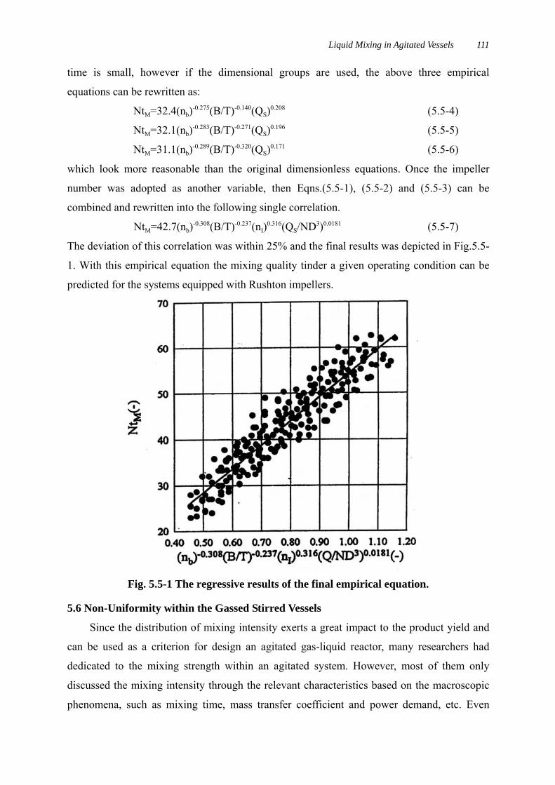
NtM=42.7(nb)-0.308(B/T)-0.237(nI)0.316(QS/ND3)0.0181 (5.5-7)
The deviation of this correlation was within 25% and the final results was depicted in Fig.5.5-
1. With this empirical equation the mixing quality tinder a given operating condition can be
predicted for the systems equipped with Rushton impellers.
Fig. 5.5-1 The regressive results of the final empirical equation.
5.6 Non-Uniformity within the Gassed Stirred Vessels
Since the distribution of mixing intensity exerts a great impact to the product yield and
can be used as a criterion for design an agitated gas-liquid reactor, many researchers had
dedicated to the mixing strength within an agitated system. However, most of them only
discussed the mixing intensity through the relevant characteristics based on the macroscopic
phenomena, such as mixing time, mass transfer coefficient and power demand, etc. Even
MULTIPLE IMPELLER GAS-LIQUID CONTACTORS112
though the mean turbulent intensity in a stirred vessel was discussed in author’s previous
works (Lu and Wang, 1986; Lu and Chen, 1986; Lu and Wu, 1988; Lu and Ju, 1996), no local
distribution of turbulent intensity, which is related to the mixing intensity, was considered,
especially for the gassed agitated system. By extending the probability theories of solid
mixing to the liquid-liquid systems, Ogawa and Ito (1975) defined a new index to identify the
quality of mixing by making use of the information entropy, and the results were applied to
the batch and steady flow systems. Ogawa et al. (1980) compared the mixing capabilities of
various impeller types using the mixing index defined by Ogawa and Ito (1975). They found
there was a basic relationship between the quality of mixing and dimensionless mixing time
Nt, and the impellers with different types give only different proportional coefficients. Ogawa
(1982) defined new local and overall mixing capacity indices based on the concept of
information entropy to discuss the distribution of mixing intensity within various single
impeller systems. In this study, the mixing capacity index defined by Ogawa (1982) were
adopted to gassed single and multiple impeller systems to examine how the gassing rate and
rotational speed will affect the mixing intensity in the agitated systems. Distributions of local
mixing capacity index, IL for different impeller combinations were also evaluated to examine
the effects of the gas dispersion capability of the impeller and the strength of liquid flow on
the mixing efficiency.
5.6.1 Theories of the mixing capacity indices
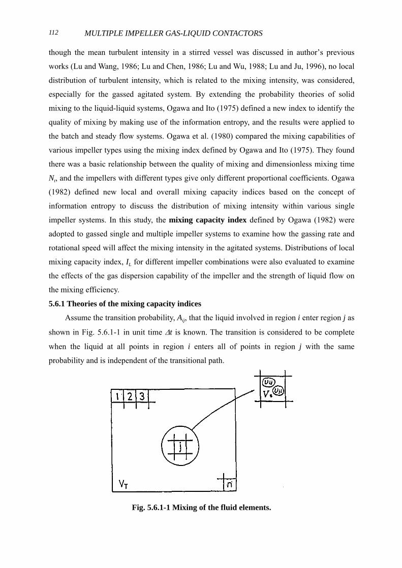
Assume the transition probability, Aij, that the liquid involved in region i enter region j as
shown in Fig. 5.6.1-1 in unit time ∆t is known. The transition is considered to be complete
when the liquid at all points in region i enters all of points in region j with the same
probability and is independent of the transitional path.
Fig. 5.6.1-1 Mixing of the fluid elements.
Liquid Mixing in Agitated Vessels 113
1. Local mixing capacity index
Liquid transports with respect to region i are divided into two parts, i.e. inflow and
outflow. The transitional probability, aij, which denotes the liquid involved in region i enter
region j of the characteristic volume VO in unit time ∆t, can be rewritten as follows:
j
Oijij V
VAa = (5.6.1-1)
The amount of information associated with the news, which informs the liquid involved in
region i enter region j of the characteristic volume VO in unit time ∆t, can be expressed as -log
aij and the probability that this news is transmitted in (Vj/VO)aij according to the information
theory. Therefore, when no news concerning the region into which the noticed liquid element
goes is transmitted, the average amount of information per the news is expected.
∑=
−=n
jijij
O
jO aa
VV
H1
1, log (5.6.1-2)
This average amount of information shows the amount of uncertainty, which is held before
the result concerning the region into which the liquid element outflow is transmitted. After the
news concerning the result is transmitted, the amount of uncertainty concerning the result
becomes zero, that is to say, the amount of information associated with the news, which
informs the region into which the liquid element outflow is expressed as:
∑=
−=−=n
jijij
O
jOO aa
VV
HI1
1,1, log 0 (5.6.1-3)
In a much similar way, the average amount of information associated with the news, which
informs the region into which the liquid element inflow can be presented as:
∑=
−=n
jjiji
O
jiI aa
VV
I1
, log (5.6.1-4)
As for the region i, from the viewpoint of mixing capacity, the exchange of liquid with more
regions with more equal probability is better than that with restricted regions with partial
probability, that is to say, the higher degree of the uncertainties described above shows a
higher mixing capacity. Assuming that the weight of outflow and inflow on the local mixing
capacity are the same, the mean value of IO,I and II,i represents the amount of local mixing
entropy of region i as:
∑=
+−=+=n
jjijiij
O
jiIOi aaa
VV
III1
ij,1, )log log(a 21)(
21 (5.6.1-5)
It is clear mathematically that this local mixing entropy takes the minimum and the maximum
MULTIPLE IMPELLER GAS-LIQUID CONTACTORS114
values as follows, respectively.
0min, =iI at aij=1 or 0 (Aij=Vj/VO or 0) (5.6.1-6)
T
Oi V
VI logmax, −= at aij=VO/VT (Aij=Vj/VT) (5.6.1-7)
The conditions described above were consistent with the statements at which the liquid in
region i is not mixed at all with the liquids in other regions and at which the liquid in region i
is mixed completely with the liquid in other regions, respectively. Considering that the
general stirring status lies between these two extreme conditions described above, the local
mixing capacity index can be defined as follows:
)/log(
)log log(a
21 1
ij
min,max,
min,,
TO
n
jjijiij
O
j
ii
iiiL VV
aaaVV
IIII
I∑=
+−=
−−
= (5.6.1-8)
In accordance with the above definition, it is aware that the local mixing capacity index varies
from 0 for complete segregation to 1 for complete mixing.
2. Overall mixing capacity index
The overall mixing entropy can be defined as the average of the local mixing entropy
weighted in accordance with the probability PV,i(=Vi/VT) as:
∑∑∑= ==
+−==n
i
n
jjijiij
TO
jin
iiVw aaa
VVVV
IPI1 1
ij1
1, )log log(a 21 (5.6.1-9)
This overall mixing capacity entropy takes the same minimum and maximum values under
identical conditions as those for the case of local mixing capacity entropy, Ii, and it is suitable
to define the overall mixing capacity index as follows:
)/log(
)log log(a
21 1 1
ij
TO
n
i
n
jjijiij
TO
ji
w VV
aaaVVVV
I∑∑= =
+−= (5.6.1-10)
Being analogous to the local mixing capacity index, the overall mixing capacity index change
from zero for no mixing state to unity for complete mixing state. The detailed procedure for
evaluating the values of IL and IW can be consulted in Ogawa (1982).
5.6.2 Distribution of local mixing capacity index
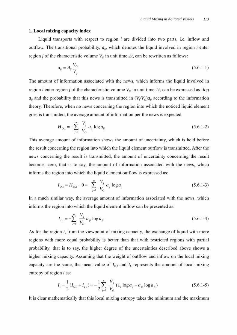
The local mixing capacity index, IL for the single Rushton turbine impeller system under
an ungassed condition with N=3.33rps was evaluated and the results are shown as a contour
map in Fig. 5.6.2-1 along with the calculated flow pattern after CFD simulation (Lu et al,
2000a). The largest value of IL always appears in the discharge stream of impeller close to
Liquid Mixing in Agitated Vessels 115
tank wall, where the discharged liquid flow changes its direction from radial to axial and
splits into two liquid circulating loops, therefore, results in larger turbulent intensity and
mixing intensity. With departing off the impeller discharge region, the turbulent intensity
decreases, which causes the decreases in IL along the liquid circulating loop and give weaker
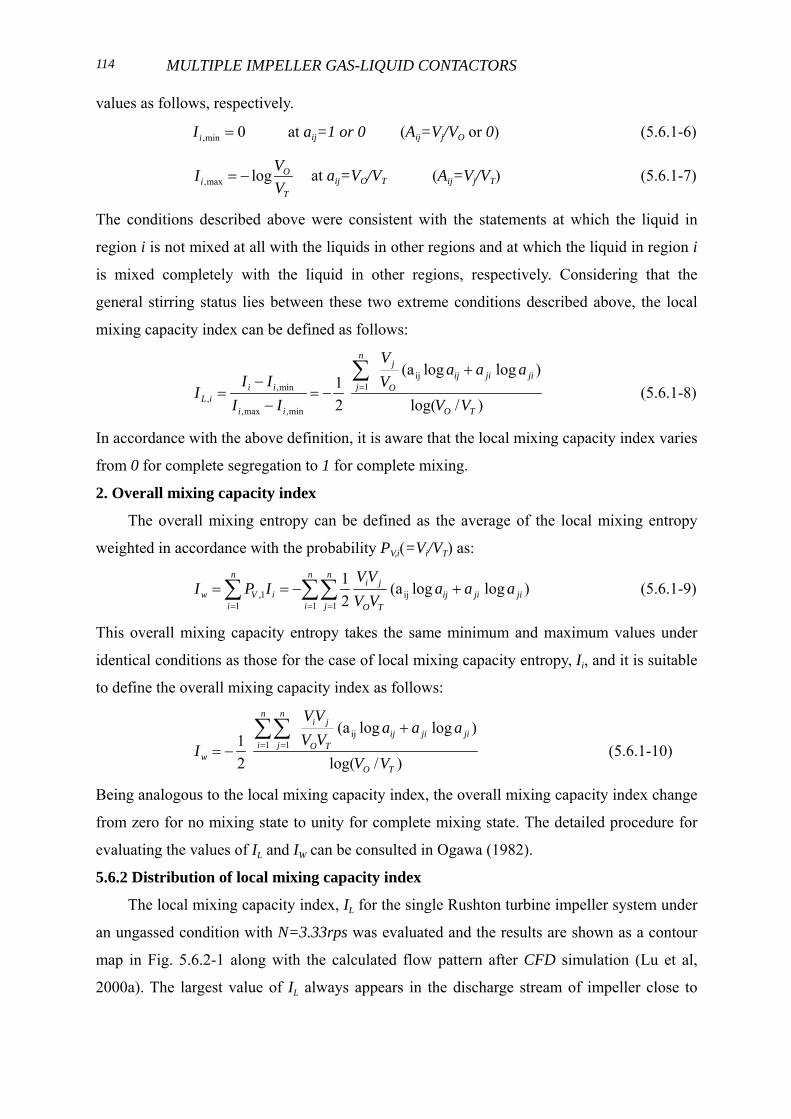
mixing intensities in the positions near the liquid surface and tank bottom. Comparing the
contour maps of IL at different R-Z planes as shown in Fig. 5.6.2-2, one can find that in the
azimuthal planes near the baffle plate, the localization of maximum IL in the discharge stream
of impeller close to tank wall will be suppressed. This phenomenon is more obvious for the
plane behind the baffle plate, which gives a more uniform distribution of IL than those in the
other two planes. According to Eq. 5.6.1-1, the overall mixing capacity index IW for the single
Rushton turbine impeller system with N=3.33rps under an ungassed condition was evaluated
as 0.484.
Fig. 5.6.2-1 Contour map of local mixing capacity index IL in the mid-plane along withthe flow pattern after Lu et al.(2000a) with N=3.33rps under an ungassedcondition.
(a) θ= +10° (b) θ= 45° (c) θ= -10°
Fig. 5.6.2-2 Comparison of the contour maps of local mixing capacity index IL in threedifferent R-Z planes with N=3.33rps (a) in front of baffle; (b) mid-plane and(c) behind baffle.
MULTIPLE IMPELLER GAS-LIQUID CONTACTORS116
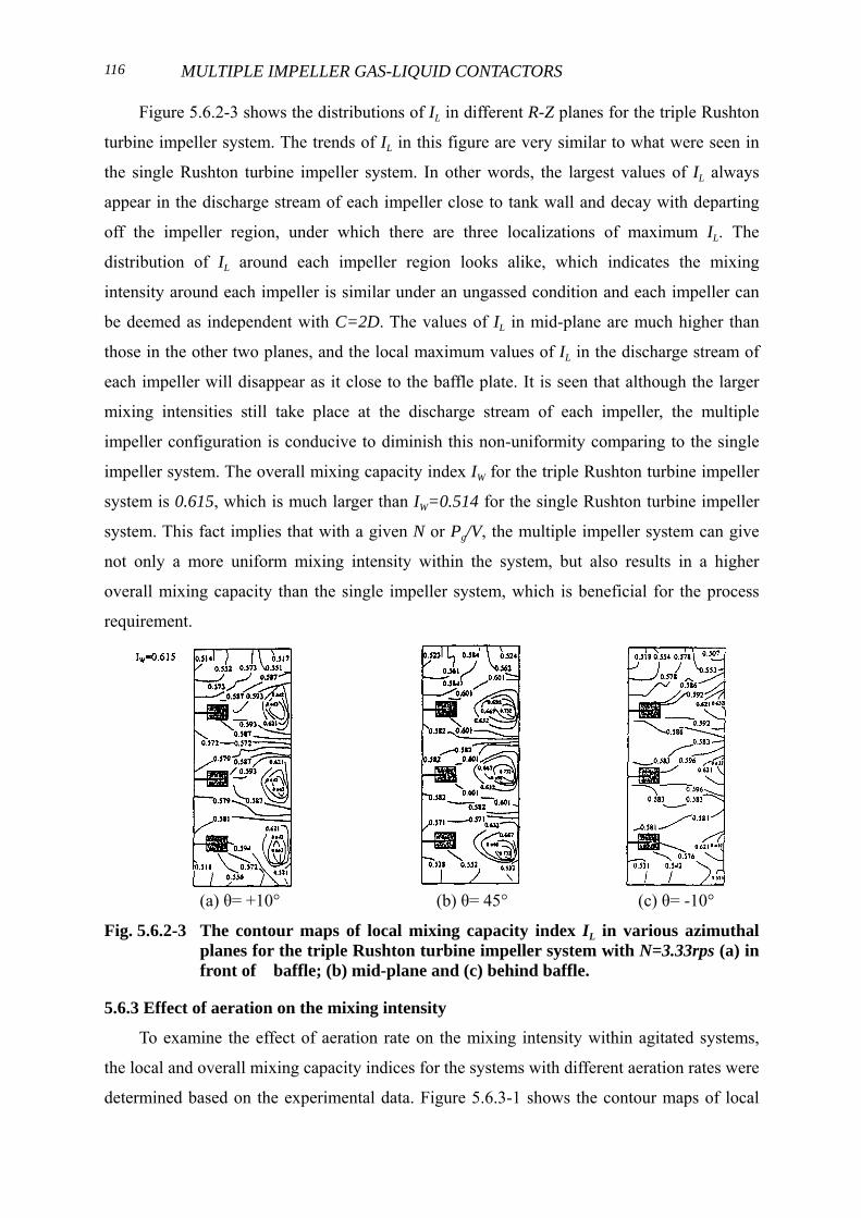
Figure 5.6.2-3 shows the distributions of IL in different R-Z planes for the triple Rushton
turbine impeller system. The trends of IL in this figure are very similar to what were seen in
the single Rushton turbine impeller system. In other words, the largest values of IL always
appear in the discharge stream of each impeller close to tank wall and decay with departing
off the impeller region, under which there are three localizations of maximum IL. The
distribution of IL around each impeller region looks alike, which indicates the mixing
intensity around each impeller is similar under an ungassed condition and each impeller can
be deemed as independent with C=2D. The values of IL in mid-plane are much higher than
those in the other two planes, and the local maximum values of IL in the discharge stream of
each impeller will disappear as it close to the baffle plate. It is seen that although the larger
mixing intensities still take place at the discharge stream of each impeller, the multiple
impeller configuration is conducive to diminish this non-uniformity comparing to the single
impeller system. The overall mixing capacity index IW for the triple Rushton turbine impeller
system is 0.615, which is much larger than IW=0.514 for the single Rushton turbine impeller
system. This fact implies that with a given N or Pg/V, the multiple impeller system can give
not only a more uniform mixing intensity within the system, but also results in a higher
overall mixing capacity than the single impeller system, which is beneficial for the process
requirement.
(a) θ= +10° (b) θ= 45° (c) θ= -10°
Fig. 5.6.2-3 The contour maps of local mixing capacity index IL in various azimuthalplanes for the triple Rushton turbine impeller system with N=3.33rps (a) infront of baffle; (b) mid-plane and (c) behind baffle.
5.6.3 Effect of aeration on the mixing intensity
To examine the effect of aeration rate on the mixing intensity within agitated systems,
the local and overall mixing capacity indices for the systems with different aeration rates were
determined based on the experimental data. Figure 5.6.3-1 shows the contour maps of local
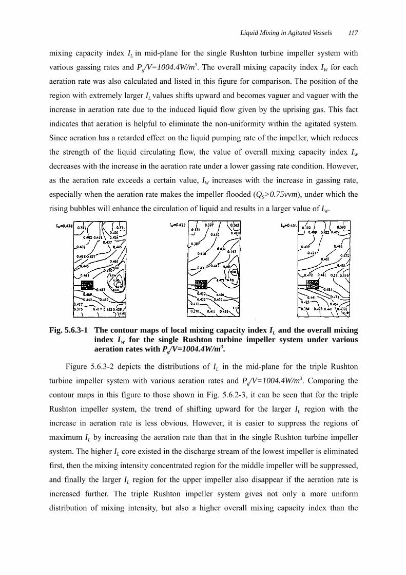
Liquid Mixing in Agitated Vessels 117
mixing capacity index IL in mid-plane for the single Rushton turbine impeller system with
various gassing rates and Pg/V=1004.4W/m3. The overall mixing capacity index IW for each
aeration rate was also calculated and listed in this figure for comparison. The position of the
region with extremely larger IL values shifts upward and becomes vaguer and vaguer with the
increase in aeration rate due to the induced liquid flow given by the uprising gas. This fact
indicates that aeration is helpful to eliminate the non-uniformity within the agitated system.
Since aeration has a retarded effect on the liquid pumping rate of the impeller, which reduces
the strength of the liquid circulating flow, the value of overall mixing capacity index IW
decreases with the increase in the aeration rate under a lower gassing rate condition. However,
as the aeration rate exceeds a certain value, IW increases with the increase in gassing rate,
especially when the aeration rate makes the impeller flooded (QS>0.75vvm), under which the
rising bubbles will enhance the circulation of liquid and results in a larger value of IW.
Fig. 5.6.3-1 The contour maps of local mixing capacity index IL and the overall mixingindex IW for the single Rushton turbine impeller system under variousaeration rates with Pg/V=1004.4W/m3.
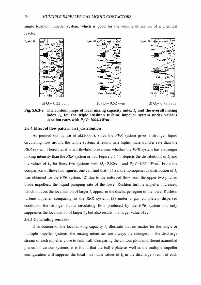
Figure 5.6.3-2 depicts the distributions of IL in the mid-plane for the triple Rushton
turbine impeller system with various aeration rates and Pg/V=1004.4W/m3. Comparing the
contour maps in this figure to those shown in Fig. 5.6.2-3, it can be seen that for the triple
Rushton impeller system, the trend of shifting upward for the larger IL region with the
increase in aeration rate is less obvious. However, it is easier to suppress the regions of
maximum IL by increasing the aeration rate than that in the single Rushton turbine impeller
system. The higher IL core existed in the discharge stream of the lowest impeller is eliminated
first, then the mixing intensity concentrated region for the middle impeller will be suppressed,
and finally the larger IL region for the upper impeller also disappear if the aeration rate is
increased further. The triple Rushton impeller system gives not only a more uniform
distribution of mixing intensity, but also a higher overall mixing capacity index than the
MULTIPLE IMPELLER GAS-LIQUID CONTACTORS118
single Rushton impeller system, which is good for the volume utilization of a chemical
reactor.
(a) Qs= 0.22 vvm (b) Qs= 0.52 vvm (d) Qs= 0.78 vvm
Fig. 5.6.3-2 The contour maps of local mixing capacity index IL and the overall mixingindex IW for the triple Rushton turbine impeller system under variousaeration rates with Pg/V=1004.4W/m3.
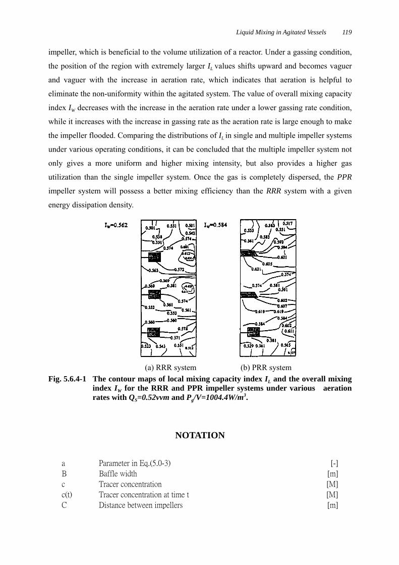
5.6.4 Effect of flow pattern on IL distribution
As pointed out by Lu et al.(2000b), since the PPR system gives a stronger liquid
circulating flow around the whole system, it results in a higher mass transfer rate than the
RRR system. Therefore, it is worthwhile to examine whether the PPR system has a stronger
mixing intensity than the RRR system or not. Figure 5.6.4-1 depicts the distributions of IL and
the values of IW for these two systems with QS=0.52vvm and Pg/V=1004.4W/m3. From the
comparison of these two figures, one can find that: (1) a more homogeneous distribution of IL
was obtained for the PPR system; (2) due to the enforced flow from the upper two pitched
blade impellers, the liquid pumping rate of the lower Rushton turbine impeller increases,
which induces the localization of larger IL appear in the discharge region of the lower Rushton
turbine impeller comparing to the RRR system; (3) under a gas completely dispersed
condition, the stronger liquid circulating flow produced by the PPR system not only
suppresses the localization of larger IL, but also results in a larger value of IW.
5.6.5 Concluding remarks
Distributions of the local mixing capacity IL illustrate that no matter for the single or
multiple impeller systems, the mixing intensities are always the strongest in the discharge
stream of each impeller close to tank wall. Comparing the contour plots in different azimuthal
planes for various systems, it is found that the baffle plate as well as the multiple impeller
configuration will suppress the local maximum values of IL in the discharge stream of each
Liquid Mixing in Agitated Vessels 119
impeller, which is beneficial to the volume utilization of a reactor. Under a gassing condition,
the position of the region with extremely larger IL values shifts upward and becomes vaguer
and vaguer with the increase in aeration rate, which indicates that aeration is helpful to
eliminate the non-uniformity within the agitated system. The value of overall mixing capacity
index IW decreases with the increase in the aeration rate under a lower gassing rate condition,
while it increases with the increase in gassing rate as the aeration rate is large enough to make
the impeller flooded. Comparing the distributions of IL in single and multiple impeller systems
under various operating conditions, it can be concluded that the multiple impeller system not
only gives a more uniform and higher mixing intensity, but also provides a higher gas
utilization than the single impeller system. Once the gas is completely dispersed, the PPR
impeller system will possess a better mixing efficiency than the RRR system with a given
energy dissipation density.
(a) RRR system (b) PRR systemFig. 5.6.4-1 The contour maps of local mixing capacity index IL and the overall mixing
index IW for the RRR and PPR impeller systems under various aerationrates with QS=0.52vvm and Pg/V=1004.4W/m3.
NOTATION
a Parameter in Eq.(5.0-3) [-]
B Baffle width [m]
c Tracer concentration [M]
c(t) Tracer concentration at time t [M]
C Distance between impellers [m]
MULTIPLE IMPELLER GAS-LIQUID CONTACTORS120
C1 Height of lower impeller from bottom [m]
D Impeller diameter [m]
H Liquid level of stirred tank [m]
L Length of impeller blade [m]
Lres Resultant turbulence scale [m]
N Impeller rotational speed [1/s]
nb Baffle number [-]
nI Impeller number [-]
np Number of impeller blade [-]
Pb Power consumption with baffle [kgm2/s3]
Pg Power consumption with aeration [kgm2/s3]
Po Power consumption without aeration [kgm2/s3]
Qs Sparged gas flow rate [m3/s]
qi,l,g Liquid volumetric flow rate between cells in the I direction [m3/s]
T Tank diameter [m]
tM Mixing time [s]
Ul,g Liquid phase velocity with aeration [m/s]
Ul,u Liquid phase velocity without aeration [m/s]
u’,v’ Fluctuation velocity [m/s]
V Liquid volume in the tank [m3]
W Mean tangential velocity [m/s]
w Impeller blade width [m]
<Greeks Letters>α Defined in Eq.(6-1)(=nbB/T) [-]
β Exponent adopted in Eq.(5.1-2) [-]
ε Energy dispersion rate [m2/s3]
εg Local gas hold-up [-]
θ Shaft angular position [degree]
κ Turbulent kinetic energy [m2/s2]
<Subscripts>g Gassed condition
i Any principle direction
i Initial condition
l Liquid phase
Pro Projective
u Ungassed condition
∞ Final condition