paper no. acom2010-xxxxx practical data of the · pdf fileuseful information for a new design...
TRANSCRIPT

Proceedings of 3rd Asian Conference on Mixing October 19-22, 2010, Jeju, Korea
Paper No. ACOM2010-xxxxx
PRACTICAL DATA OF THE HEAT TRANSFER COEFFICIENT AT THE INSIDE WALL OF AN AGITATED VESSEL
Zauyah Zamzam*1, Hisayuki Kanamori1, Takashi Yamamoto1 and Yoshikazu Kato1 1Mixing Technology Laboratory
Satake Chemical Equipment MFG. LTD., Saitama, Japan 335-0021
* E-mail: [email protected]
ABSTRACT
In this study, a new method presented by Kanamori et al. was practically used to determine the heat transfer coefficient at the
inside wall of an agitated vessel in the high mixing Reynolds number region. The impellers used are a 3-bladed propeller, a 4-
bladed pitched paddle and a 6-bladed flat turbine of the conventional impellers and Satake Supermix MR210 of the large impeller.
The characteristics of each impeller were made clear based on the experimental results by investigated the effects of the impeller
speed, baffling conditions (2-baffled and non-baffled) and the impeller positions on the heat transfer coefficient.
Moreover, a new information concerning about the relations of the flow pattern and flow velocity distribution on the heat
transfer coefficient was also clarified. Finally, it is expected that the new heat transfer coefficient measuring method present the
useful information for a new design of mixing device.
INTRODUCTION Heat transfer in agitated vessels is a common industrial
practice that has been researched extensively. Heat transfer
operation plays important roles on the mixing device such as:
1. Heat elimination on the chemical reaction.
2. Fluid temperature control on the crystallization.
3. Fluid temperature rising on the dissolution process.
and others. Generally, the accuracy of the temperature measurement
in the range of high Reynolds numbers may depend on how to
set the thermocouple. Rigorous methods of temperature
measurement were investigated. Traditionally, many workers
employed the extrapolation method by inserting two or more
thermocouples inside the vessel wall [2], [4], [5] and setting the
thermocouple on the surface of the vessel wall which is
trenched inside the channel [5].
The main purpose of this paper is to presents the
practical data of the heat transfer coefficient at the inside wall
of an agitated vessel by using a new heat transfer coefficient
measuring method presented by Kanamori et al. This new
measuring method is simple and is expected to be more
practical and more precise that enables to provide an effective
measurement application for the mixing device in the future. Additionally, this work is also to make clear the
relationship between the heat transfer coefficient distributions
with the flow velocity distribution and the flow pattern inside
agitated vessels. In order to achieve these purpose:
1. The heat transfer coefficient distribution (h distribution)
is determined by using a new measuring method
experimentally.
2. The relationship between the h distribution and the flow
velocity is investigated.
3. The effect of the flow pattern inside agitated vessels on
the h distribution at the vessel wall is identified.
in a wide range of experimental conditions and impeller
designs.
EXPERIMENTAL METHODS AND DEVICES 1.1 Experimental Devices Fig. 1 is a schematic diagram of the experimental device.
The vessel diameter was Φ250mm and the height of the liquid
in the vessel was 325mm. Experiments were carried out under
a condition of steady state heat transfer in which steam
(1070C) was fed into the jacket and overflowed and water
(500C, 6L/min.) was fed inside the vessel and overflowed.
The volume of the water inside the vessel was kept constant.
There were five measuring points at the vicinity of the vessel
wall, as shown in Fig. 1. The heat transfer coefficients were
measured at these five measuring points. A summary of the
experimental conditions; baffling conditions, impeller
positions and impeller speed are shown in Table 1.
The flow velocity distribution and the flow pattern inside
agitated vessels were measured by using the experimental
device shown in Fig. 2. The vessel was made of a transparent
acrylic resin with a diameter of Φ240mm. Water was used as
an experimental medium inside the vessel. Particle tracers for
L.D.V. (Laser Doppler Velocimetry) and P.T.V. (Particle
Tracking Velocimetry) were Expancel and Nylon 12 in micro
order, which are in spherical shapes. The density of these
particle tracers are almost similar with the water used. For the
light sheet, an Argon-ion laser was used.
In P.T.V. [1], [3] each particle tracers were tracked by using
four time steps that later detected by using the tracking
algorithm. High performance speed of CCD Camera (100f/s)
was used to record multiple images of the moving particles.
The P.T.V. measurement was set at (a) overall view : (240×
270)mm, (b) vicinity to the vessel wall : (90×145)mm and (c)
vessel bottom : (120×147)mm as shown in Fig. 3.
The flow velocity, V was evaluated by using the
following Eq. (1):
V = [(Vz)2+(Vθ)2]1/2 (1)

(a)(a)
(b)(b)(c)(c)
Laser
High Speed
CCD Camera
100 (fps)
Laser
TC
(a)(a)
(b)(b)(c)(c)
Laser
High Speed
CCD Camera
100 (fps)
Laser
TC
(i) Front View (ii) Upper View
Fig. 1 Experimental device Fig. 2 P.T.V. and L.D.V. system Fig. 3 P.T.V. analysis cross-section
In the above equation, Vz and Vθ is the component of
the axial and tangential velocity, respectively. The measuring
points were 6mm from the vessel wall.
1.2 Experimental Materials
Besides the conventional impellers, Satake Supermix
impeller of MR210 with Φ156mm in diameter and 264mm in
height was also used as the representative of the large
impeller. The clearance of the impeller and the vessel bottom
was set at 5mm.
Three types of conventional impellers were used; 4-
bladed pitched paddle (4PP), 3-bladed propeller (3P) and 6-
bladed flat turbine (6FT) with Φ96mm in diameter.
Table 1 Experimental conditions
Baffling conditions 2-baffled
Non-baffled
Impeller positions, C/d [-] 0.5
1.0
1.2
Impeller speed, N [min-1] 120
180
240
300
360
RESULTS AND DISCUSSIONS
1. Results discussions in 2-baffled agitated vessels
1.1 The effect of the impeller positions
1.1.1 Heat transfer coefficient distribution Figs. 4, 5 and 6 show the effect of the impeller positions
on the heat transfer coefficient distribution (h distribution) in
the axial direction at the vessel wall in 2-baffled agitated
vessels for 3P, 4PP and 6FT, respectively. In the case of 3P
and 4PP, the h distribution is the highest at the impeller
position is located at 0.5 with the maximum h distribution is
obtained at the tangential level (T.L.).
In contrary, the highest h distribution is obtained at the
impeller position is located at 1.0 for 6FT, although there is a
slightly declination at the T.L.
1.1.2 Flow velocity distribution In order to clarify the relationship between h distribution
and flow velocity, the flow velocity was measured by
changing the impeller positions. Figs. 7, 8 and 9 show the
results obtained for 3P, 4PP and 6FT, respectively. It is well
understood that in the case of 3P and 4PP, the flow velocity is
apparently highest at the impeller position is located at 0.5.
Moreover, the flow velocity is also almost identical at the
impeller positions are located at 1.0 and 1.2.
Regardless of the impeller positions, the flow velocity
showed a slightly declination at the T.L. This may probably
indicated that the main flow may occupied by the radian
velocity than the tangential velocity at this point. However,
the flow velocity is almost constant at the impeller position is
located at 1.0 for 6FT. In contrary, wide range of flow
velocity is obtained at the other impeller positions.
1.1.3 Flow pattern In order to make clear on the effect of the flow pattern on
the h distribution, the flow pattern is visualized by changing
the impeller positions. Figs. 10 and 11 illustrate the flow
pattern for 3P and 4PP at the impeller position is located at
0.5. It is clearly observed that a strong axial flow is discharged
by the blades and strike the vessel wall with sharp angle at the
T.L. for both impellers. This sharp angle is noticed to provide
greater affect to the thermal boundary layer at the vessel wall.
Subsequently, maximum h distribution is obtained at the T.L.
Fig. 12 illustrates the flow pattern for 6FT at the impeller
position is located at 1.0. Two complete circulating zones are
generated with the radial discharged flow by the blades strike
the vessel wall with a sharp angle at the vessel bottom near to
the T.L. Therefore, maximum h distribution is obtained at this
point. However, since the impeller position is farther away
from the vessel bottom, less flow attack to the vessel wall at
the T.L. is considered to be the main factor contributed to the
decreases in h distribution at this point.
1.2 The effect of the impeller speed
1.2.1 Heat transfer coefficient distribution
Figs. 13, 14, 15 and 16 display the effect of the impeller
speed on the h distribution for 3P, 4PP, 6FT and MR210,
respectively. It is well observed that h distribution is
dependent on the impeller speed for these impellers. The h
250
200
150
100
50
(T.L.)
d
C
Steam
inlet
Steam
outlet Water
outlet
Measuring
points
H [mm]
Baffle
Water
outlet
Jacket’s pressure
0.13MPa
(107℃)
Water inlet
(50℃, 6L/min.)
D
250
200
150
100
50
(T.L.)
d
C
Steam
inlet
Steam
outlet Water
outlet
Measuring
points
H [mm]
Baffle
Water
outlet
Jacket’s pressure
0.13MPa
(107℃)
Water inlet
(50℃, 6L/min.)
D LDV System
Digital Burst
Correlator
Argon ion
LASER
Driver
PCDigital Torque
Meter
ARGON
LASER
CCD Camera
Satake
PTV System
Spectroscopic
Instrument
3-Axis
Controller
LASER
Sheet
3-Axis
Traverse Unit
Torque DetectorDigital Burst
Correlator
LDV System
Digital Burst
Correlator
Argon ion
LASER
Driver
PCDigital Torque
Meter
ARGON
LASER
CCD Camera
Satake
PTV System
Spectroscopic
Instrument
3-Axis
Controller
LASER
Sheet
3-Axis
Traverse Unit
Torque DetectorDigital Burst
Correlator

0
50
100
150
200
250
300
350
0.0 0.5 1.0 1.5 2.0 2.5 3.0
Dis
tan
ce f
rom
bo
tto
m
H [
mm
]
h [W/cm2K]
C = 0.5d
C = 1.0d
C = 1.2d
0
50
100
150
200
250
300
350
0.0 0.5 1.0 1.5 2.0 2.5 3.0
Dis
tan
ce f
rom
bo
tto
m
H [
mm
]
h [W/cm2K]
C = 0.5d
C = 1.0d
C = 1.2d
0
50
100
150
200
250
300
350
0.0 0.5 1.0 1.5 2.0 2.5 3.0
Dis
tan
ce f
rom
bo
tto
m
H [
mm
]
h [W/cm2K]
C = 0.5d
C = 1.0d
C = 1.2d
0
50
100
150
200
250
300
350
0.0 0.1 0.2 0.3 0.4 0.5 0.6 0.7 0.8 0.9 1.0
Dis
tan
ce f
rom
bo
tto
m
H [
mm
]
C=0.5d
C=1.0d
C=1.2d
V [m/s]
0
50
100
150
200
250
300
350
0.0 0.1 0.2 0.3 0.4 0.5 0.6 0.7 0.8 0.9 1.0
V [m/s]
Dis
tan
ce f
rom
bo
tto
m
H [
mm
]
C=0.5d
C=1.0d
C=1.2d
0
50
100
150
200
250
300
350
0.0 0.1 0.2 0.3 0.4 0.5 0.6 0.7 0.8 0.9 1.0
V [m/s]
Dis
tan
ce f
rom
bo
tto
m
H [
mm
]
C=0.5d
C=1.0d
C=1.2d
0
50
100
150
200
250
300
350
0.0 0.5 1.0 1.5 2.0 2.5 3.0
120min-1
180min-1
240min-1
300min-1
360min-1
h [W/cm2K]
Dis
tan
ce f
rom
bo
tto
m
H[m
m]
3P 4PP 6FT
MR210 MR210
0
50
100
150
200
250
300
350
0.0 0.5 1.0 1.5 2.0 2.5 3.0
Dis
tan
ce f
rom
bo
tto
m
H[m
m]
120min-1
180min-1
240min-1
300min-1
360min-1
h [W/cm2K]
0
50
100
150
200
250
300
350
0.0 0.5 1.0 1.5 2.0 2.5 3.0
Dis
tan
ce f
rom
bo
tto
m
H[m
m]
120 min-1
180 min-1
240 min-1
300 min-1
360 min-1
h [W/cm2K]
3P 4PP 6FT
3P 4PP 6FT
Figs. 4, 5, 6 H vs. h (from left: 3P, 4PP, 6FT) under the effect of impeller position
Figs. 7, 8, 9 H vs. V (from left: 3P, 4PP, 6FT) under the effect of the impeller position
Figs. 10, 11, 12 Flow pattern (from left: 3P, 4PP, 6FT)
Figs. 13, 14, 15 H vs. h (from left: 3P, 4PP, 6FT) under the effect of impeller speed
Fig. 16, 17 From left: H vs. h, H vs. V under the effect of impeller speed Fig. 18 Flow pattern of MR210
(C/d = 0.5)
0
50
100
150
200
250
300
350
0.0 0.5 1.0 1.5 2.0 2.5 3.0
37 min-1
73 min-1
110 min-1
147 min-1
184 min-1
Dis
tan
ce f
rom
bo
tto
m
H[m
m]
h [W/cm2K]
0
50
100
150
200
250
300
350
0.0 0.1 0.2 0.3 0.4 0.5 0.6 0.7 0.8 0.9 1.0
V [m/s]
Dis
tan
ce f
rom
bo
tto
m
H [
mm
]
37 min-1
73 min-1
110 min-1
134 min-1

0
50
100
150
200
250
300
350
0.0 0.5 1.0 1.5 2.0 2.5 3.0
h [W/cm2K]
Dis
tan
ce f
rom
bo
tto
m
H [
mm
]
4PP
6FT
0
50
100
150
200
250
300
350
0.0 0.5 1.0 1.5 2.0 2.5 3.0
Dis
tan
ce f
rom
bo
tto
m
H [
mm
]
h [W/cm2K]
4PP
MR210
distribution spreads wider as approaching to the T.L. and the
maximum h distribution is obtained at the T.L. This indicated
that the higher the impeller speed showed a good tendency to
obtain higher h distribution.
1.2.2 Flow velocity distribution The effect of the impeller speed on the flow velocity for
MR210 is shown in Fig. 17. The flow velocity is increases as
the impeller speed increased.
1.2.3 Flow pattern The effect of the flow pattern on the h distribution is
investigated for MR210, as shown in Fig. 18. For MR210, a
large circulation flow is generated and the strong flow from
the vessel bottom gets along the vessel wall closely. This flow
characteristic of MR210 contributes to the constant flow
velocity thoroughly in the agitated vessel.
Furthermore, a sharp angle flow strikes at the T.L. which
exhibits greater affect to the thermal boundary layer thickness
that provided maximum h distribution at the T.L.
1.3 Comparative data at constant C/d and constant Pv
1.3.1 Heat transfer coefficient distribution
Fig. 19 and 20 show the comparative results of 4PP and
6FT, 4PP and MR210 at Pv = 0.2 [kW/m3] and C/d = 0.5
constant, respectively. The h distribution is almost similar at
most of the measuring points except at the vessel bottom
position near to the T.L., which the h distribution is greater for
4PP than 6FT.
Meanwhile, comparing to 4PP, the h distribution is
almost constant for MR210. However, h distribution is
increased profoundly at T.L. and vessel bottom position near
to the T.L. for 4PP.
1.3.2 Flow velocity distribution
The flow velocity for 4PP and 6FT, 4PP and MR210 are
shown in Fig. 21 and 22, respectively. From these results, it is
well understood that the flow velocity is greater for 4PP than
6FT at the vessel bottom position near to the T.L. However, in
the case of 4PP and MR210, the flow velocity showed almost
constant value for MR210 than 4PP.
1.3.3 Flow pattern
The flow pattern for 4PP and 6FT are shown in Fig. 11
and 23, respectively. From these flow patterns, it is well
observed that both of these impellers produced mainly the
axial flow. However, flow velocity is greater for 4PP than 6FT
at the vessel bottom position near to the T.L., which was
obtained in the previous result. This indicated that a strong
axial flow was generated for 4PP than 6FT at this point.
Therefore, maximum h distribution is obtained for 4PP.
The flow pattern for 4PP and MR210 are displayed in
Fig. 11 and 18, respectively. From these flow patterns, a large
circulation flow generated by MR210 is observed to exhibit a
more constant h distribution and constant flow velocity
thoroughly inside agitated vessels.
In contrary, a strong short pass of axial flow produced by
4PP at the T.L. and vessel bottom position near to the T.L.
that provided significant affect to the increases in the intensity
of turbulence at the thermal boundary layer. Therefore, h
distribution is profoundly increased at these points.
Fig. 19 H vs. h (4PP and 6FT)
Fig. 20 H vs. h (4PP and MR210)
Fig. 21 H vs. h (4PP and 6FT)
Fig. 22 H vs. V (4PP and MR210)
Fig. 23 Flow pattern of 6FT
(C/d = 0.5)
0
50
100
150
200
250
300
350
0.0 0.1 0.2 0.3 0.4 0.5 0.6 0.7 0.8 0.9 1.0
4PP
6FT
V [m/s]
Dis
tan
ce f
rom
bo
tto
m
H [
mm
]
0
50
100
150
200
250
300
350
0.0 0.1 0.2 0.3 0.4 0.5 0.6 0.7 0.8 0.9 1.0
V [m/s]
Dis
tan
ce f
rom
bo
tto
m
H [
mm
]
4PP
MR210
3P 4PP 6FT
3P 4PP 6FT
0
50
100
150
200
250
300
350
0.0 0.5 1.0 1.5 2.0 2.5 3.0
h [W/cm2K]
Dis
tan
ce f
rom
bo
tto
m
H [
mm
]
C = 0.5d
C = 1.0d
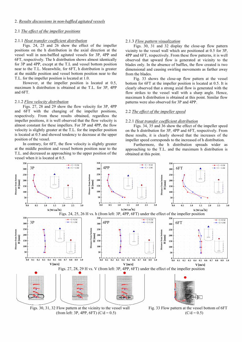
2. Results discussions in non-baffled agitated vessels
2.1 The effect of the impeller positions
2.1.1 Heat transfer coefficient distribution
Figs. 24, 25 and 26 show the effect of the impeller
positions on the h distribution in the axial direction at the
vessel wall in non-baffled agitated vessels for 3P, 4PP and
6FT, respectively. The h distribution shows almost identically
for 3P and 4PP, except at the T.L and vessel bottom position
near to the T.L. Meanwhile, for 6FT, h distribution is greater
at the middle position and vessel bottom position near to the
T.L. for the impeller position is located at 1.0.
However, at the impeller position is located at 0.5,
maximum h distribution is obtained at the T.L. for 3P, 4PP
and 6FT.
2.1.2 Flow velocity distribution
Figs. 27, 28 and 29 show the flow velocity for 3P, 4PP
and 6FT with the changing of the impeller positions,
respectively. From these results obtained, regardless the
impeller positions, it is well observed that the flow velocity is
almost constant for these impellers. For 3P and 4PP, the flow
velocity is slightly greater at the T.L. for the impeller position
is located at 0.5 and showed tendency to decrease at the upper
position of the vessel.
In contrary, for 6FT, the flow velocity is slightly greater
at the middle position and vessel bottom position near to the
T.L. and decreased as approaching to the upper position of the
vessel when it is located at 0.5.
2.1.3 Flow pattern visualization
Figs. 30, 31 and 32 display the close-up flow pattern
vicinity to the vessel wall which are positioned at 0.5 for 3P,
4PP and 6FT, respectively. From these flow patterns, it is well
observed that upward flow is generated at vicinity to the
blades only. In the absence of baffles, the flow created is two
dimensional and causing swirling movements as farther away
from the blades.
Fig. 33 shows the close-up flow pattern at the vessel
bottom for 6FT at the impeller position is located at 0.5. It is
clearly observed that a strong axial flow is generated with the
flow strikes to the vessel wall with a sharp angle. Hence,
maximum h distribution is obtained at this point. Similar flow
patterns were also observed for 3P and 4PP.
2.2 The effect of the impeller speed
2.2.1 Heat transfer coefficient distribution
Figs. 34, 35 and 36 show the effect of the impeller speed
on the h distribution for 3P, 4PP and 6FT, respectively. From
these results, it is clearly showed that the increases of the
impeller speed corresponds to the increased of h distribution.
Furthermore, the h distribution spreads wider as
approaching to the T.L. and the maximum h distribution is
obtained at this point.
0
50
100
150
200
250
300
350
0.0 0.5 1.0 1.5 2.0 2.5 3.0
h [W/cm2K]
C = 0.5d
C = 1.0d
Dis
tan
ce f
rom
bo
tto
m
H [
mm
]
0
50
100
150
200
250
300
350
0.0 0.5 1.0 1.5 2.0 2.5 3.0
h [W/cm2K]
C = 0.5d
C = 1.0d
Dis
tan
ce f
rom
bo
tto
m
H [
mm
]
Figs. 24, 25, 26 H vs. h (from left: 3P, 4PP, 6FT) under the effect of the impeller position
0
50
100
150
200
250
300
350
0.0 0.1 0.2 0.3 0.4 0.5 0.6 0.7 0.8 0.9 1.0
Dis
tan
ce f
rom
bo
tto
m
H [
mm
]
C=0.5d
C=1.0d
V [m/s]
0
50
100
150
200
250
300
350
0.0 0.1 0.2 0.3 0.4 0.5 0.6 0.7 0.8 0.9 1.0
V [m/s]
Dis
tan
ce f
rom
bo
tto
m
H [
mm
]
C=0.5d
C=1.0d
0
50
100
150
200
250
300
350
0.0 0.1 0.2 0.3 0.4 0.5 0.6 0.7 0.8 0.9 1.0
V [m/s]
Dis
tan
ce f
rom
bo
tto
m
H [
mm
]
C=0.5d
C=1.0d
Figs. 27, 28, 29 H vs. V (from left: 3P, 4PP, 6FT) under the effect of the impeller position
Figs. 30, 31, 32 Flow pattern at the vicinity to the vessel wall
(from left: 3P, 4PP, 6FT) (C/d = 0.5)
Fig. 33 Flow pattern at the vessel bottom of 6FT
(C/d = 0.5)

0.01
0.1
1
10
0.01 0.1 1 10
V [m/s]
h [
W/c
m2K
]
Keys
Black : non-baffled
Red : 2-baffled
Green : 4-baffled
Various impellers
・6FT ・3P ・4PP
・Pfeudler ・HR100
・HR320 ・HS604
・MR210 ・MR203
0.01
0.1
1
10
0.01 0.1 1 10
V [m/s]
h [
W/c
m2K
]
Keys
Black : non-baffled
Red : 2-baffled
Green : 4-baffled
Various impellers
・6FT ・3P ・4PP
・Pfeudler ・HR100
・HR320 ・HS604
・MR210 ・MR203
3P 4PP 6FT
3. Relationship between the heat transfer distribution and the flow velocity
Up to here, the effects of the impeller designs, impeller
positions and impeller speed on the h distribution inside an
agitated vessel were made clear. In order to clarify the
relationship between the h distribution and the flow velocity,
h distribution is plotted against the flow velocity as shown in
Fig. 37. It is made clear that at the T.L., the relationship
between the h distribution and the flow velocity get almost a
linear line. However, as the clearance between the impeller
and the vessel bottom become wider, wide variance were
obtained.
This result may give sufficient information for scaling-up
works in the future.
Fig. 37 Relationship between h distribution and flow velocity
for various impellers, baffled and non-baffled
conditions
CONCLUSIONS 1. Practical data on the h distribution at the inside wall of
agitated vessels by using a new measuring method were
verified by experimental results.
2. The effects of the impeller design, impeller positions and
impeller speed on the h distribution at the inside wall of
agitated vessels were made clear.
3. The effects of the flow pattern and the flow velocity were
identified to gives greater affect on the h distribution in
agitated vessels.
UNITS AND SYMBOLS C = clearance between impeller and the
vessel bottom
[mm]
D = diameter of the agitated vessel
[mm]
d
= diameter of impeller
[mm]
H
h
N
= distance from the vessel bottom
= heat transfer coefficient at the inside
wall
= impeller speed
[mm]
[W/cm2K]
[min-1]
V = flow velocity
[m/s]
Vz = axial velocity [m/s]
Vθ = tangential velocity
[m/s]
Pv = power number per unit volume [kW/m3]
REFERENCES [1] Kanamori, H., Kobayashi, T., Saga, T. and Segawa S., 1990,
“Flow Visualization and Analisys of Chemical Agitated Vessel by
Particle Imaging Velocimetry,” Journal of the Visualization Society
of Japan, Vol. 10, No. 2, 239-242
[2] Kuriyama, M., Ohta, M., Yanagawa, K., Arai, K. and Saito, S.,
1981, “Heat transfer and temperature distributions in an agitated
tank equipped with helical ribbon,” Journal of Chemical Engineering
of Japan, Vol. 14, No. 4, 323-330
[3] Kobayashi, T., Saga, T., Lee, Y. and Kanamori, H., 1991, “Flow
visualization and analysis of 3-D square cavity and mechanically
agitated vessels by Particle Imaging Velocimetry,” 3rd Triennial
International Symposium on Fluid Control, Measurement, and
Visualization ’91, 401-406
[4] Mitsuishi, N., Miyairi, Y. and Katamine, T., 1973, “Heat
transfer to a Newtonian liquids in an agitated vessel,” Journal of
Chemical Engineering of Japan, Vol. 6, No. 5, 409-414
[5] Mizushina, T., Ito, R., Murakami, Y. and Kiri, M., 1966,
“Experimental Study of Newtonian Fluid to the wall of an agitated
vessel,” Kagaku Kougaku, Vol. 30, No. 8, 719-726 [6] Nagata, S., Nishikawa, M., Takahiro, T., Kida, F. and Kayama,
T., 1971, “Jacket Side Heat Transfer Coefficient in Mixing Vessel,”
Kagaku Kougaku, Vol. 35, No. 8, 924-932
Figs. 34, 35, 36 H vs. h (from left: 3P, 4PP, 6FT) under the effect of the impeller speed
0
50
100
150
200
250
300
350
0.0 0.5 1.0 1.5 2.0 2.5 3.0
120min-1
180min-1
240min-1
300min-1
360min-1
h [W/cm2K]
Dis
tan
ce f
rom
bo
tto
m
H[m
m]
0
50
100
150
200
250
300
350
0.0 0.5 1.0 1.5 2.0 2.5 3.0
h [W/cm2K]
120min-1
180min-1
240min-1
300min-1
360min-1
Dis
tan
ce f
rom
bo
tto
m
H [
mm
]
0
50
100
150
200
250
300
350
0.0 0.5 1.0 1.5 2.0 2.5 3.0
120min-1
180min-1
240min-1
300min-1
360min-1
h [W/cm2K]
Dis
tan
ce f
rom
bo
tto
m
H[m
m]