telemark university college - upcommons · telemark university college faculty of technology...
TRANSCRIPT

Telemark University College Faculty of Technology
Bachelor of Engineering
Faculty of Technology
Address: Kjølnes ring 56, N-3918 Porsgrunn, Tel: +47 35 02 62 00, www.hit.no
Bachelor’s programmes – Master’s programmes – PhD programmes
REPORT FOR 6TH SEMESTER PROJECT SPRING 2015
PRH612 Bacheloroppgave
K6-4-15
Bachelor Student’s Project
Evaluating and Designing Systems for Mixing Water in Oil

Høgskolen i Telemark Fakultet for teknologiske fag
Bachelor i ingeniørfag
Høgskolen tar ikke ansvar for denne studentrapportens resultater og konklusjoner
Fakultet for teknologiske fag
RAPPORT FRA 6. SEMESTERS PROSJEKT VÅREN 2015
Emne: PRH612 Bacheloroppgave
Tittel: Evaluating and Designing Systems for Mixing Water in Oil
Rapporten utgjør en del av vurderingsgrunnlaget i emnet.
Prosjektgruppe: K6-4-15 Tilgjengelighet: Åpen
Gruppedeltakere:
Anders Galland Andersen
June Kanton
Jane Marlen Sanna
Ana Vicente
Hovedveileder: Lars E. Øi Sensor: Kjell-Arne Solli
Biveileder: Kjell-Arne Solli Prosjektpartner: Steve Watson Gabriel
Godkjent for arkivering:
Sammendrag: Olje- og gassindustrien består av utforsking, uthenting, oppgradering, separering, raffinering,
transportering og markedsføring av oljeprodukter. Etter separeringsprosessen er vann fjernet i stor grad,
og kun en liten andel gjenstår i råoljen. Når produktene markedsføres, er verdien essensiel, og på grunn
av dette må det tas en representativ prøve for å fastslå kvaliteten. Dette krever at vanndråpene er
uniformt fordelt i oljen når den evalueres.
FMC Technologies forespurte et miksesystem som kunne oppnå en homogen strømning i et rør, for en
rekkevidde av parametere. Ettersom en laminær strømning er mest utfordrende å blande, blir
parameterene som gir det laveste Reynolds tallet valgt til videre evaluering.
Litteraturstudier viser at det finnes flere metoder å oppnå en uniform blanding på. Blandetank, statisk
miksing, og power miksing ble analysert. Statiske miksere ble evaluert basert på dagens teknologi, og et
power miksing system ble designet for lavest mulig Reynolds tall. For å kunne evaluere metodene ble
det utført beregninger, og det ble oppdaget at blandetanken ikke er egnet for miksing i rør. Den ble
derfor ikke evaluert videre.
Trykktap er økonomisk ugunstig, og dette blir tatt hensyn til når konklusjonen diskuteres. Statisk
miksing er anbefalt når Reynolds tallet er under 2000, og diameteren i hovedrøret er mindre enn 0,4 m.
Ingen miksing er nødvendig når Reynolds tallet når et visst punkt, da strømningen vil bli såpass
turbulent at den vil mikses naturlig. Power miksing er anbefalt for alle andre definerte tilfeller.

Telemark University College Faculty of Technology
Bachelor of Engineering
Telemark University College does not accept any responsibility for the results or
conclusions of this student report
Faculty of Technology
REPORT FOR 6TH SEMESTER PROJECT SPRING 2015
Course: PRH612 Bacheloroppgave
Title: Evaluating and Designing Systems for Mixing Water in Oil
This report is a part of the evaluation result for the course.
Project group: K6-4-15 Accessibility: Open
Group participants:
Anders Galland Andersen
June Kanton
Jane Marlen Sanna
Ana Vicente
Principal supervisor: Lars E. Øi Examiner: Kjell-Arne Solli
Co-supervisor: Kjell-Arne Solli Project partner: Steve Watson Gabriel
Approved for archiving:
Summary:
The oil and gas industry includes the processes of exploration, extraction, upgrading, separation,
refining, transporting and marketing oil products. After the separation process, water is removed to a
great extent, and only a small percentage is left in the crude oil. When marketing the products, the value
is essential, and therefore a representative sample has to be extracted to determine the quality. This
requires that the water is uniformly distributed throughout the batch when it is evaluated.
FMC Technologies requested a mixing system that would be able to achieve a homogeneous flow in a
pipeline, for a range of parameters. Because a laminar flow is the most challenging to mix, the
parameters which gives the lowest Reynolds number are chosen as a worst case scenario.
By literature studies, it is stated that a uniform mixture can be provided by multiple processes.
Mechanically agitated vessels, static- and power mixing have been analyzed. The static mixer is
evaluated based on the state of the art, and a power mixing system is designed for the worst case
parameters. Calculations are performed to be able to evaluate. It is found that mechanically agitated
vessels are not recommended for in-line mixing and therefore not evaluated further.
Pressure drop is expensive, and this is taken into account when discussing a conclusion. A static mixer
is recommended for Reynolds numbers below 2000 and a main pipe diameter below 0.4 m. No mixing
is required when the Reynolds number reaches a certain peak where the turbulence in the flow is of a
large extent and mixing will happened naturally. Otherwise, power mixing is the suggested method to
provide a homogeneous flow.

Telemark University College Facultad de tecnología
Grado en ingeniería
Telemark University College no acepta ninguna responsabilidad de los resultados o las
conclusions de este trabajo
Facultad de tecnología
TRABAJO DEL 6TO SEMESTRE PROYECTO PRIMAVERA 2015
Curso: PRH612 Bacheloroppgave
Titulo: Evaluating and Designing Systems for Mixing Water in Oil
Este trabajo es una parte del resultado de la evaluación del curso.
Grupo del proyecto: K6-4-15 Disponibilidad: Abierta
Miembros del grupo:
Anders Galland Andersen
June Kanton
Jane Marlen Sanna
Ana Vicente
Supervisor: Lars E. Øi Examinador: Kjell-Arne Solli
Co-supervisor: Kjell-Arne Solli Asociado del projecto: Steve Watson Gabriel
Aprobado para su archivo
Resumen:
En la industria del petróleo y el gas natural se incluyen los procesos de explotación, extracción, mejora,
refinamiento, transporte y comercialización de los productos derivados del petróleo. Después del
proceso del proceso de separación, el agua es eliminada en su mayor parte, sólo un pequeño porcentaje
permanece en el crudo. En la comercialización de los productos derivados, conocer las características
del crudo es esencial, y por tanto la muestra extraída para determinar su calidad tiene que ser
representativa. Esto requiere que el agua este distribuida uniformemente en toda la sección en el
momento de su valoración.
FMC Technologies encomendó un sistema de mezcla en interior de la tubería que fuera capaz de
proporcionar un flujo homogéneo para un rango de parámetros. Los parámetros que proporcionan un
menor número de Reynolds son los escogidos como peor caso, debido a que el flujo laminar es más
difícil de mezclar.
Como afirman diferentes estudios de la literatura, una mezcla uniforme puede ser proporcionada por
múltiples procesos. Los métodos de mezclado analizados son el tanque agitado, mezclador estático y
mezclador JetMix. El mezclador estático es evaluado en base al estado del arte, y el sistema JetMix es
diseñado para los parámetros del peor escenario posible. Para su evaluación diversos cálculos han sido
realizados. El tanque agitado no está evaluado en profundidad porque no es el más recomendado para
mezclar en interior de una tubería.
La pérdida de carga es cara, por lo que es esencial en la discusión de las conclusiones. Se recomienda
un mezclador estático para números de Reynolds por debajo de 2.000 y un diámetro tubería principal
por debajo de 0.4 m. No se requiere de mezclador cuando el número Reynolds alcanza un cierto valor
donde la turbulencia en el flujo es muy elevada y la mezcla sucede de manera natural. En cualquier otro
caso, mezclador JetMix es el método sugerido para proporcionar un flujo homogéneo.

Høgskolen i Telemark Preface
K6-4-15 3
PREFACE
This project was performed by four students at Telemark University College, during the 6th
and
final semester of an undergraduate degree. Three of the students are studying Gas- and Energy
Technology and are accompanied by an exchange student from Polytechnic University of
Catalonia, studying Chemical Engineering. The report is written in collaboration with FMC
Technologies, a market leader in design, manufacture and supply of measurement products and
systems for the oil and gas industry worldwide.
The team is grateful for the guidance provided by Steve Watson Gabriel, our contact person from
FMC. The team would also like to thank Arve Langeland and Nils Petter Aaastad for their
guidance and feedback.
The front page picture is an illustration of the designed power mixing system made in
SolidWorks.
This report was made using standard Microsoft Office programs and SolidWorks.
It is expected of the reader to have basic knowledge of fluid mechanics.
Porsgrunn, 26.05.2015:
Ana Vicente
Anders Galland Andersen
June Liavik Kanton
Jane Marlen Sanna

Høgskolen i Telemark Glossary
K6-4-15 4
GLOSSARY
Symbol Term Unit
Q Flow rate in main pipe m3/s
A Area of main pipe m2
D Diameter of main pipe m
Di Inner diameter of main pipe m
V Main pipe velocity m/s
Density of mixture kg/m3
Viscosity Pa*s
P Pressure in main pipe Pa, bar
T Temperature °C
g Gravitational acceleration kg/s2
Lm Mixing length m
KL, KT Pressure drop ratios for motionless mixers Dimensionless
KiL, KiT Mixing rate coefficient for blending Dimensionless
CoV Coefficient of variation Dimensionless
Pp Pressure drop empty pipe Pa
Pressure drop static mixer Pa
Re Reynolds number Dimensionless
f Friction factor Dimensionless
Density difference in oil and water kg/m3
Fr’ Froude’s number Dimensionless
Head needed from the pump m
Head loss m
v1 Velocity of the fluid before the pump m/s
v2 Velocity of the fluid after the pump m/s

Høgskolen i Telemark Glossary
K6-4-15 5
K Minor loss coefficient factor Dimensionless
U Saybolt Universal viscosity at a given temperature SSU
Cv Flow coefficient Dimensionless
q Flow rate in the power mixing loop m3/h
Lv Length of vertical pipe in the power mixer m
LH Length of horizontal pipe in the power mixer m
Lpm Length of total pipe in the power mixer m
NRE Reynolds number of the worst case parameters Dimensionless
v Velocity in recycle pipe m/s
Apm Area of recycle pipe m2
d Diameter recycle pipe m
d0 Outside diameter of probe m
di Inside diameter of probe m
dre Diameter of the nozzle outlet m
Are Area of the nozzle outlet m2
St Strouhal Number Dimensionless
fm Factor Dimensionless
L Allowable length m
z1 Elevation in main pipeline m
z2 Elevation in nozzle m
ΔZ Elevation difference of probe and nozzle m
C1 Concentration of water on the top of main pipe %
C2 Concentration of water in the bottom of the main pipe %
vre Velocity of re-injection m/s
Kinematic viscosity mm2/s
Turbulence characteristics m/s

Høgskolen i Telemark Glossary
K6-4-15 6
G Parameter dependent on degree of mixing Dimensionless
W Settling rate of water droplets m/s
Water density kg/m3
Crude oil density kg/m3
Er Required energy dissipation W/kg
P Pressure drop Bar
E Young’s Modulus of Elasticity Pa
Pn Pressure in nozzle Pa
X Distance of homogeneous flow m
t Temperature
xw Water concentration %
xo Crude oil concentration %

Høgskolen i Telemark Table of Content
K6-4-15 7
TABLE OF CONTENT
Preface ................................................................................................................................... 3
Glossary ................................................................................................................................ 4
Table of Content ................................................................................................................... 7
1 Introduction ..................................................................................................................... 9
2 Background for the Project .......................................................................................... 10
3 Mixing Methods ............................................................................................................. 11
3.1 Static Mixing........................................................................................................................................ 11 3.2 Power Mixing ...................................................................................................................................... 13 3.3 Mechanically Agitated Vessels ........................................................................................................... 15
3.3.1 Evaluation of the Method ............................................................................................................ 16
4 Problem Description ..................................................................................................... 18
5 Sampling ......................................................................................................................... 19
5.1 Automatic Pipeline Sampling ............................................................................................................. 19 5.1.1 Profile Testing.............................................................................................................................. 19 5.1.2 Design and Position of Sampling Probe ..................................................................................... 20 5.1.3 Sampling Loop ............................................................................................................................. 23
6 Evaluating Static Mixing .............................................................................................. 24
6.1 Worst-Case Scenario........................................................................................................................... 24 6.1.1 Mixer Orientation ........................................................................................................................ 25 6.1.2 Calculating Mixing Length and Pressure Drop ......................................................................... 26 6.1.3 Slight Variations in Process Parameters for the Worst-Case Scenario ..................................... 28
6.2 Varying Parameters ............................................................................................................................ 28 6.2.1 Pipe Diameter .............................................................................................................................. 28 6.2.2 Density and Water Cut................................................................................................................. 30 6.2.3 Viscosity ....................................................................................................................................... 30 6.2.4 Velocity ......................................................................................................................................... 31 6.2.5 All Parameters ............................................................................................................................. 33
7 Design of a Power Mixing System ................................................................................ 35
7.1 Process Description ............................................................................................................................. 35 7.2 Utilities ................................................................................................................................................. 36
7.2.1 Probe ............................................................................................................................................ 36 7.2.2 Nozzle ........................................................................................................................................... 37 7.2.3 Pump ............................................................................................................................................ 40 7.2.4 Valves ........................................................................................................................................... 40 7.2.5 Elbows .......................................................................................................................................... 41 7.2.6 Filter ............................................................................................................................................. 41 7.2.7 Piping ........................................................................................................................................... 43 7.2.8 Sizing the Pump ........................................................................................................................... 45
8 Evaluating Power Mixing ............................................................................................. 47
8.1 Worst Case Scenario ........................................................................................................................... 47 8.2 Varying Parameters ............................................................................................................................ 48
8.2.1 Pipe Diameter .............................................................................................................................. 48 8.2.2 Velocity ......................................................................................................................................... 51 8.2.3 Density .......................................................................................................................................... 51 8.2.4 Viscosity ....................................................................................................................................... 53 8.2.5 All Parameters ............................................................................................................................. 54
9 Discussion ....................................................................................................................... 55

Høgskolen i Telemark Table of Content
K6-4-15 8
9.1 Uncertainties ........................................................................................................................................ 55 9.2 Recommended Solutions ..................................................................................................................... 56 9.3 Suggestions for Further Work ........................................................................................................... 57
10 Conclusion ...................................................................................................................... 58
Referance ............................................................................................................................ 59
Appendix ............................................................................................................................. 61

Telemark University College
K6-4-15 9
1 INTRODUCTION
After refining oil from the welds, the oil will contain some percentage of unwanted components.
These components will be removed in separation processes, and the final product will contain a
small percentage of water. To determine the quality of the oil, a representative sample has to be
provided. This can be done by mixing the product before sampling.
FMC Technologies requested a design of a power mixing system, or an alternative economical
solution which meets the requirements. The scope of the project is changed to evaluation and
design of systems for mixing water in oil. The goal of the project is to recommend a mixing
system for a defined case, as well as comparing methods for a range of parameters. The task
from FMC can be found in Enclosure A.
The design and evaluation are based on literature studies and calculations performed in the
report. No simulations will be performed during this project, therefore all results will be strictly
theoretical.
The project limits are set by FMC, as a range of parameters. Values outside this range will not be
taken into consideration. In addition to this, the focus is directed towards the mixing- and
sampling station. The data from FMC can be found in Enclosure B.
Chapter 2 consists of a thorough description of the background for the problem.
In chapter 3, different mixing methods for solving this problem are presented.
The scope of the project is further explained in chapter 4.
The process of how to provide a representative sample is evaluated in chapter 5.
In chapter 6, static mixing is evaluated.
In chapter 7, a power mixing system is designed and later evaluated in chapter 8.
The results, uncertainties and suggestions for further work are discussed in chapter 9, before the
final conclusions are presented in chapter 10.

Telemark University College
K6-4-15 10
2 BACKGROUND FOR THE PROJECT
Many operations depend to a great extent on effective mixing of fluids. Mixing refers to any
operation used to change a non-uniform system into a uniform one. Mixing is an integral part of
chemical or physical processes such as blending, dissolving, dispersion, suspension,
emulsification, heat transfer, and chemical reactions.
The oil and gas industry includes the processes of exploration, extraction, upgrading, separating,
refining, transporting and marketing oil products. When the liquid is extracted from an oil field,
it consists primarily of hydrocarbons and other organic compounds. It may also contain various
gases, solids, trace materials and water. The liquid is refined and separated to consumer
products. In this separation process, it is impossible to remove all the unwanted components. [1][2]
When refined oil is to be purchased or sold, the value varies with the quality. When determining
a price, the water content is an essential factor. The higher the water cut, the lower percentage of
oil per volume, and the lower the value.
Oil and water are immiscible liquids. This is because hydrogen bonds can’t be formed when
water molecules are polar and oil molecules are non-polar. To circumvent this fact, the water
needs to be mixed into the oil so that it is equally distributed throughout the batch. Only then the
true amount of water can be determined. [3]
Consequently, the purpose of mixing is to determine the amount of water and other components
in the oil, and thereby the quality. Mixing plays an important role for product sampling in the
pipeline transport, and has to be installed upstream of the sampler. Adequate mixing should
create a good dispersion but still allow water to easily settle in downstream storage tanks.
After mixing water and oil, a sample that is representative for the whole batch is required to
prove the quality of the product. This can only be accomplished by extraction of samples from a
homogeneous mixture of the batch. This is achieved when the water droplets are of equal size,
with equal distances to each other so they don’t coagulate, and uniformly distributed throughout
the area of the container.
To ensure that the samples are representative is important for all the companies that are involved.
Therefore, it is absolutely important to make sure that the sampling process is of a high standard.
Several parameters are critical to ensure this, including placement, extraction point, treatment of
the sample and time intervals between sampling. [1]

Telemark University College
K6-4-15 11
3 MIXING METHODS
Most of the general information about mixing methods is from reference [4].
Mixing is a unit operation where a heterogeneous fluid is made homogeneous. To achieve a
homogeneous mixture the heterogeneous fluid will be stirred to the point where it has the same
composition throughout the batch. There are not only liquids that can be mixed; solids and
gasses are also fluids that can be blended if the right equipment is used. Different types of
materials that can be mixed are:
Liquid-liquid mixing
Gas-gas mixing
Solid-solid mixing
Liquid-solid mixing
Liquid-gas mixing
Gas-solid mixing
Solid, liquid, and gas mixing
For this project the only relevant mixing type is liquid-liquid mixing, because both water and oil
are liquids. Single-phase and multiphase mixing are the two different types of liquid-liquid
mixing.
Single-phase blending is when the liquids are miscible or at least soluble in each other. The
liquids will dissolve easily in one another when both of them are water based. When both liquids
have a low viscosity, the momentum of the liquid being added is sufficient to cause enough
turbulence to mix the two. When the liquids have a higher viscosity it is necessary to use a
stirring device to complete the mixing process.
Multiphase mixing is when the liquids are not soluble or miscible in each other. Water and oil is
an example of multiphase mixing. When blending water and oil, it’s necessary to use a mixing
device to achieve a homogenous mixture, which will start to separate if it’s not continually
mixed.
There are different ways to mix a multiphase fluid. The fluid can either be mixed in a vessel or
while it is flowing through a pipeline. In this chapter three different methods for mixing the oil
and water will be described. The three mixing methods that will be evaluated are mechanically
agitated vessels, static- and power mixing. The two most suited methods for the worst case
parameters will be studied in depth before a final conclusion will be made.
3.1 Static Mixing
Information about this subject has been collected from source [5].
Static mixers, also known as motionless mixers, are mixing devices which consist of elements
inserted into a pipe. In that way a process fluid flows through a pipe and is redirected multiple
times by various mixing elements placed inside the pipe. An example of how this affects the
flow is shown in Figure 3-1 below. There are many different types of mixing elements, but all of
them are stationary in use. This is an advantage as the result is practically no need for
maintenance, in addition to having very low operating costs. This method of mixing is very
flexible, as it is possible to include multiple mixing elements, based on the difficulty of the
mixing task.

Telemark University College
K6-4-15 12
Figure 3-1: Mixing efficiency using GXM mixing elements [6]
Static mixers are used in both laminar and turbulent processes. Laminar flow mixing consists of
a combination of flow division and re-orientation. In turbulent flow mixing, the mixing elements
create a higher level of turbulence than in an otherwise empty pipe.
A common type of static mixing is the packed column used in distillation processes. In this
column, water and gas is being mixed by directing the flows through small openings inside a
tube, of which an example is shown in Figure 3-2. As with any other static mixers, the type of
packing inside the tube varies from column to column, and is easily replaced. A thing to note
about the packed column is that the flows are countercurrent, whereas the static mixer usually
handles co-current mixing problems.

Telemark University College
K6-4-15 13
Figure 3-2: Example of a packed column used in distillation. [7]
One of the problem-areas of the static mixers is the pressure drop they create. The only driving
force in this mixing process is the pressure inside the pipe, and as the fluid flows through the
mixing elements, the pressure will drop. Therefore it is important to make sure that the operating
pressure never drops below the vapor pressure for the specific fluid.
3.2 Power Mixing
For this chapter reference [9], [10] and [11] are used.
Power mixing is when an external power device is used to achieve a satisfying mixture. The
power mixer system removes a portion of the liquid from the main pipe and re-injects it under
pressure. A probe is used to remove a small portion of the fluid from the main pipe and into the
mixing loop. Inside the mixing loop a pump will provide the necessary pressure for the fluid to
get re-injected back into the main pipe, and to prevent back flow. The re-injection is done
through a nozzle, which is designed to create as much turbulence as possible in the main pipe.
Figure 3-3 is an illustration of how a power mixing system is constructed.

Telemark University College
K6-4-15 14
Figure 3-3: Illustration of Power Mixing. [8]
Because of the difference in densities for water and oil, they will start separating after the mixing
process. The gravitational force will cause the water to appear as slugs inside the pipe and sink to
the bottom of a horizontal pipe. When the fluid is flowing upstream in a vertical pipe the velocity
of the oil will be slightly higher than the velocity of the water. This is because the density of
water is higher and the gravitational force will make it harder for the water to move upwards. In
a vertical pipe where the fluid is flowing downstream it will be the opposite; the water will be
transported faster downwards than the oil. The gravitational force will affect the separation
between the water and oil less in the vertical pipe than in the horizontal pipe.
Because the gravity has an effect on the separation of the water and oil it is important that the
quality of the oil is measured when the flow is still homogeneous.
When deciding the type of mixer that should be used for a certain process the pros and cons for
each type of mixing system should be evaluated.
When constructing the power mixer, the capital cost will be large compared to the static mixer.
The reason for the high expenses when purchasing a power mix system is the equipment needed
such as the different utilities and piping.
Another disadvantage for the power mix system is that the operating cost will be higher than in
the static mixer. The operating cost in the power mixing system is caused by the power
consumption from the pump.
An advantage of the power mixer is that it will work for all different ranges in parameters. At
some point the flow inside the pipeline will have a turbulent flow where the water and oil
naturally mixes by itself. A benefit for the power mixer is that it can be shut off and save the
operational expenses.
The power mix system will be less secure than a static mixer because the system depends on a
pump. If there is any damage to the pump that requires maintenance, the system has to be shut
down until the pump is functional again.
The pressure drop of the fluid inside the power mix system will be small compared to the static
mixer. Elements that will cause the pressure to decrease through the mixing loop are valves,
elbows, probe, filter and pipe surface. The pressure drop caused by these utilities will be
significantly lower than drop caused by the obstructions in the static mixer.

Telemark University College
K6-4-15 15
3.3 Mechanically Agitated Vessels
Most of the information in this chapter is from the references [12] and [13].
Mixing refers to any operation used to change a non-uniform system into a uniform one.
Particularly agitation implies forcing a fluid by mechanical means to flow in a circulatory or
other pattern inside a vessel.
The basic components to take into account in a design of a mechanically agitated vessel are the
tank, the impeller and the baffles. Figure 3-4 illustrates a basic design with the size relationships
that the different elements should meet.
Geometric portions for
standard agitation system:
·
·
·
·
·
·
Figure 3-4: Standard tank configuration (6 blade turbine with 4 symmetrical baffles).
The top of the vessel may be open or sealed, the vessel bottom is normally not flat but rounded
to eliminate sharp corners or regions into which the fluid currents would not penetrate. Dished
ends are most common, because they require less power than flat ends. Baffles are needed to
prevent vortexing and rotation of the liquid mass as a whole, except at high Reynold numbers.
Impellers are the most important components to change when designing for different
applications. In general, they can be classified in two main groups:
- Impellers with a small blade area, which rotate at high speeds, are used to mix low to
medium viscosity liquids. These include turbines and marine propellers.
- Impellers with a large blade area, which rotate at low speeds, are effective for high-
viscosity liquids. These include anchors, paddles, and helical screws.
In Figure 3-5, the most common types of impellers used today are illustrated.

Telemark University College
K6-4-15 16
Turbine Marine propeller Anchor Paddle Helical scew
Figure 3-5: Different kinds of impellers. [14]
The properties of the liquid and the dimensions and arrangement of impellers, baffles and other
internals are factors that influence the amount of energy required for achieving a required
amount and quality of agitation. For that reason, the power consumed by a stirred tank depends
on: Type of impeller and its size and geometry, characteristics of the fluid and rotation speed of
the stirrer.
Process requirements vary widely. Some applications require homogenization at near molecular
level, while other objectives can be met as long as large scale convective flows sweep through
the whole vessel volume. Performance is crucially affected both by: the nature of the fluids
concerned and on how quickly the mixing or dispersion operation must be completed.
In the studied case, oil and water are two immiscible liquids which are not easily blended. For
this case turbine impellers is the most suitable stirrer to provide the desired mixing conditions for
immiscible liquids.
3.3.1 Evaluation of the Method
Mechanically agitated vessel is a well-known method because it has been used for a long time.
Moreover it can be used for a wide range of applications by only changing the main design (for
example the kind of impeller or the dimensions of the tank), that is why it is a flexible method.
On the other hand, it also has some disadvantages: The power consumption is high because it is
necessary to make an impeller rotate with a constant speed. Moreover, as it is not wished to
create a stable emulsion, the design of this mixing system should be very accurate. If the two
liquids are not blended enough, after the stirring the crude oil and water, the small drops of water
will join again and the two liquids will split up. However, if the two liquids are blended too
much a stable emulsion could be obtained.
This method is usually performed in a tank, but in-line mixing is possible. A version of this is
stirring the mixture inside the pipe by simply adding an impeller like it is shown in Figure 3-6.

Telemark University College
K6-4-15 17
Figure 3-6: Impeller stirring the liquids driven inside a pipe. [15]
This option is not an effective one: When blending easy miscible liquids of similar viscosities, an
agitator will produce satisfactory results. On the other hand, when there is a significant
difference in viscosity between the two liquids, an agitator tends to move them around without
actually blending them together and it can take a long time to achieve a uniform mixture.
These devices could give short blend times or high local energy dissipations. To overcome this
problem, horizontal baffles are added and the liquids are blended in two steps. This type of in-
line mechanical mixer is called rotatory in-line blenders as illustrated in Figure 3-7.
Figure 3-7: Rotatory in-line blender. [12]
This blender is installed in an oversized section of the pipe in order to increase residence time
and reduce superficial velocity. More than two stages can be used to provide more accurate
residence time. The design consists of at least two stages, each with an impeller, and internal
baffles. The incoming flow is forced to pass through each stage with strategically designed
baffles before exiting.
This mixer works most efficiently at low flow rates when mixing is most needed. When the flow
rate is high, the mixer can be turned off to prevent formation of a stable emulsion.

Telemark University College
K6-4-15 18
4 PROBLEM DESCRIPTION
The main goal of this project is to provide FMC Technologies with a suggestion of the most
reasonable mixing method and sampling method for their process. A range of parameters from
previous projects was provided, and the range is listed in Table 4-1.
Table 4-1: Historical data from FMC Technologies. [16]
Parameter
Value
Unit
Minimum Maximum
Header Velocity 0.15 15.43 m/s
Density 600 1000 kg/m3
Viscosity 0.4 100 Cp
0.0004 0.1 Pa·s
Pressure 0 100 Barg
Temperature - 150 ᵒC
Water Cut 0.5 5 %
Header Size Range 6 30 "
0.1536 0.768 m
Reynolds number is a dimensionless value used to describe the flow characteristics of a fluid and
the tendency to experience a considerable amount of viscous drag. The importance of the
Reynolds number is that it determines what flow regimes will exists for fluids of known density
and absolute viscosity traveling at a given velocity. The lower the value, the more laminar the
flow, and it is calculated by Equation (4.1).
(4.1)
In a laminar flow the fluid particles move in a straight parallel line in such a way that individual
particles do not cross the path of neighboring particles. When the turbulence in the flow
increases, this is no longer the case. The movement of the particles will be in a more random
manner resulting in a natural mixing of the fluid. Because of this, a laminar flow is the most
difficult to mix properly, and the parameters that gives the lowest value of Reynolds number are
chosen when evaluating the mixing systems. According to Equation (4.1), this corresponds to the
lowest density, pipe diameter and velocity and the highest viscosity, as highlighted in Table 4-1.
FMC requested in-line mixing, which makes the mechanically agitated vessel less applicable.
Because of this, coupled with the high power consumption, the mechanically agitated vessel was
deemed unfit for this problem and will not be evaluated further. [16]

Telemark University College
K6-4-15 19
5 SAMPLING
Most of the information in this chapter is based on international standard 3171. [1]
Hydraulic laws are important regarding the behavior of the heterogeneous liquids, which will
mix in the pipe. It is proved that if the stream conditions that results in a sufficiently high energy
dissipation rate are met, the drops of water will be kept suspended in the crude oil. This energy
dissipation can be provided by mixing, in this case, static- or power mixing.
A representative sample is defined as a sample having its physical and chemical characteristics
identical to the average characteristics of the total volume being sampled. In other words, when
the mixture is homogeneous, as defined in chapter 2. There are four conditions that must be met:
1. The samples should have the same composition as the average composition of the crude
oil over the whole cross-section of the pipeline at the location and time of sampling.
2. The rate of sampling should be in proportion to the flow rate in the pipe.
3. The sample should be maintained in the same condition as in the point of extraction.
4. When dividing the sample into sub-samples, it must be done in such a way that ensures
each of the sub-samples to have the same composition of the original sample.
There are two main types of sampling systems. One of which is in-line sampling, where a probe
is placed and samples are grabbed directly. This method is the simplest system available, but
offers the lowest accuracy and highest uncertainty. Fast-loop sampling is the other main system
on the market, where the sample is taken inside the pipeline in a bypass loop. This is a more
expensive and complicated system, but will thereby provide a higher accuracy. These two
systems including CoJetix- sampling represents the state of the art in sampling technology. A
CoJetix system is a sampler combined with a power mixing system, and this system provides the
lowest uncertainty of all sampling systems available. [17]
Within the systems, either manual- or automatic sampling is installed. If the homogeneous
liquids composition and quality do not vary with time, manual sampling would be adequate.
Otherwise automatic pipeline sampling is recommended.
In this case, no variations with time cannot be guaranteed because an undispersed phase can
occur. A peak with relatively high concentration of water can travel down the pipeline at some
time depending on the uploading procedure. To ensure that the sampling system designed is
suitable for multiple processes, automatic pipeline sampling will be recommended instead of
manual sampling. By choosing this sampling method, continuous or repetitive extraction of
small samples ensures that any changes in the bulk, including peaks, are reflected in the samples. [19]
5.1 Automatic Pipeline Sampling
In this chapter, the design of a sampling station that will ensure a representative sample will be
presented. Automatic pipeline sampling is the method suggested to be used in the sampling
process, and the sample location, probe, and ratio are important parameters that will be
evaluated.
5.1.1 Profile Testing
By performing profile testing, a test of the uniformity of water dispersion across the pipeline at a
possible sampling location is determined. It is recommended to perform five of these tests to
ensure uniformity.

Telemark University College
K6-4-15 20
The figures above illustrates different profiles that can be found by profile testing. In case 3 and
4, illustrated in Figure 5-3 and Figure 5-4, the concentration across the cross-section is non-
linear, and a range of different concentrations of water exists throughout the pipeline. Therefore,
with this profile, it is not possible to extract a representative sample at any location.
For case 2, as in Figure 5-2, there is a uniform gradient but yet the concentration varies from one
point to another across the cross-section area. There is at least one point where a representative
sample could be extracted, but sampling will only be representative within limits.
The purpose of mixing is to achieve the concentration profile 1 as illustrated in Figure 5-1. In
this case, the concentration is the same within the acceptable limits across the entire cross-
section of the pipeline. In other words, small water droplets are equally distributed the conditions
are acceptable for sampling.
5.1.2 Design and Position of Sampling Probe
The linear velocity and direction of the liquid flowing into the opening of the probe has to be
equal to the linear velocity and direction of the main pipeline. This is because, if the sampling
Figure 5-1: Concentration profile case 1 Figure 5-2: Concentration profile case 2
Figure 5-4: Concentration profile case 4 Figure 5-3: Concentration profile case 3

Telemark University College
K6-4-15 21
velocity is less than the fluid velocity, particles will typically not enter the sampling tube. If the
sampling velocity is higher, suction will occur and more particles will enter the probe compared
to the amount that are continuing with the main flow. In this case, the particles are the water
droplets and maybe some trace components. This is termed isokinetic sampling, and the probe
has to be designed in such a way that this is taken into account.
The length the probe can be inserted into the main pipe without failure due to the effects of
resonant vibrations has to be considered. Resonant vibrations occur when the fluid flows past
obstructions, like a probe, by formation of vortex shedding which creates a pressure drop on that
side of the obstruction. Thereby the probe will tend to bend towards this lower-pressure side
which can lead to crack formation and ultimately failure. The length allowable without the
possibility for cracks can be calculated according to Equation (5.1). [19]
√
(
) (5.1)
The factor fm equals 0.9 for liquids, and the Strouhal Number St is dependent on the shape of the
probe and the Reynolds number of the process flow. With a Reynolds number of the value up to
105 and a circular probe, the Strouhal Number is roughly constant at 0.2, which is the case in the
major part of the given range in chapter 4. These values are substituted into Equation (5.2). [19]
√
√
(
) (5.2)
Recommended diameter of the sampling probe is larger than 6 mm, somewhat dependent on the
main pipe diameter. By assuming a thickness of 1 mm, the allowable length can be calculated,
and the parameters and results for the design of the probe are listed in Table 5-1. [1]
Table 5-1: Parameters and values for the calculations of probe length.
Symbol Value Unit
d0 0.007 m
di 0.006 m
V 0.15 m/s
E 1.8822*1011
Pa
600
kg/m3
L 2 m
The allowable length is larger than the main pipe diameter, and the probe can be placed at any
point in the main pipe without any chance for failure. The most suited position of the sampling
probe is within the area where the two liquids are most likely to be well mixed at all times,
which depends on the mixing orientation. This area is illustrated as the grey zone in Figure 5-5
for a vertical pipe and Figure 5-6 for a horizontal pipe. [1]

Telemark University College
K6-4-15 22
Figure 5-5: Well-mixed zone of the main pipe, vertical orientation.
Figure 5-6: Well-mixed zone of the main pipe, horizontal orientation.
For main pipe diameters above 300 mm, five or more sampling points should be constructed. For
pipe diameters below 300 mm, as in this case 153.6 mm, three sampling points are
recommended. To be able to perform profile testing, a probe is needed at the bottom and top of
the pipe. The conclusion is to place three probes, two for profile testing and one for sampling.
Recommended distances from the mixing device and the probes are at least three- and preferably
greater than five pipe diameters, depending on mixing method, which determines the settling rate
of the average-sized water droplets. It is important that the probe is placed within the distance

Telemark University College
K6-4-15 23
where separation has not yet occurred, as when water droplets are settling. It should also be
taken into account that swirl and asymmetry is generated by the mixing device, unrepresentative
sampling can be avoided by not placing the probe too close to the device. On these grounds, it is
suggested to place the sampling probe on a distance of eight pipe diameters from the mixing
nozzle.
5.1.3 Sampling Loop
A sample loop is a by-pass to the main pipeline. A representative portion of the total flow is
circulated through the sampling loop and by this way transported back to the main pipeline.
Figure 5-7: Horizontal fast loop sampling. [18]
With fast loop transport of the sample, as illustrated in Figure 5-7, rapid response to process
changes are achieved and valuable liquid waste are avoided. It requires less differential pressure
than the alternative; single line transport, and is appropriate for liquid samples when the tap-to-
analyzer line is of a certain length. The time-delay associated with sample systems will also be
kept to a minimum with this kind of sampling system. A fast loop system can also run at higher
flow rate than a single-line configuration. [19][20]
When the mixing occurs in a vertical pipe, the sampling loop should be of a horizontal
orientation, and vice versa.
An intermittent sampler, which contains a system for extraction of liquid from the flowing
stream in the pipeline, should be installed in the loop. There is a sample received and the
sampling frequency and grab volume are regulated in relation to the flow rate. The sum of the
grabs represents one sample. Strictly speaking, the grab volume and sampling frequency are
dependent on the flow rate. [1]
Telemark University College
K6-4-15 24
6 EVALUATING STATIC MIXING
In this chapter, static mixing will be evaluated for the worst-case scenario as well as for the
entire range of parameters given by FMC. Two prominent types of static mixers will be
compared, and a suggestion will be made as to which of the types are recommended for the
worst-case scenario, as well as for the entire range of parameters.
6.1 Worst-Case Scenario
A static mixer, as explained in chapter 3.1, is a very simple mixing method that does not require
any additional piping or equipment, other than the mixing elements themselves. As a result of
this, the process looks similar to that of a fluid flowing through an empty pipe, with the only
difference being the obstructions inside the pipe.
Different types of static mixers use different types of mixing elements to blend the fluid either
radially, or by use of flow reorientation. Both of these methods have proven to be effective,
when applied correctly. Because there are so many different types of static mixers, it can be
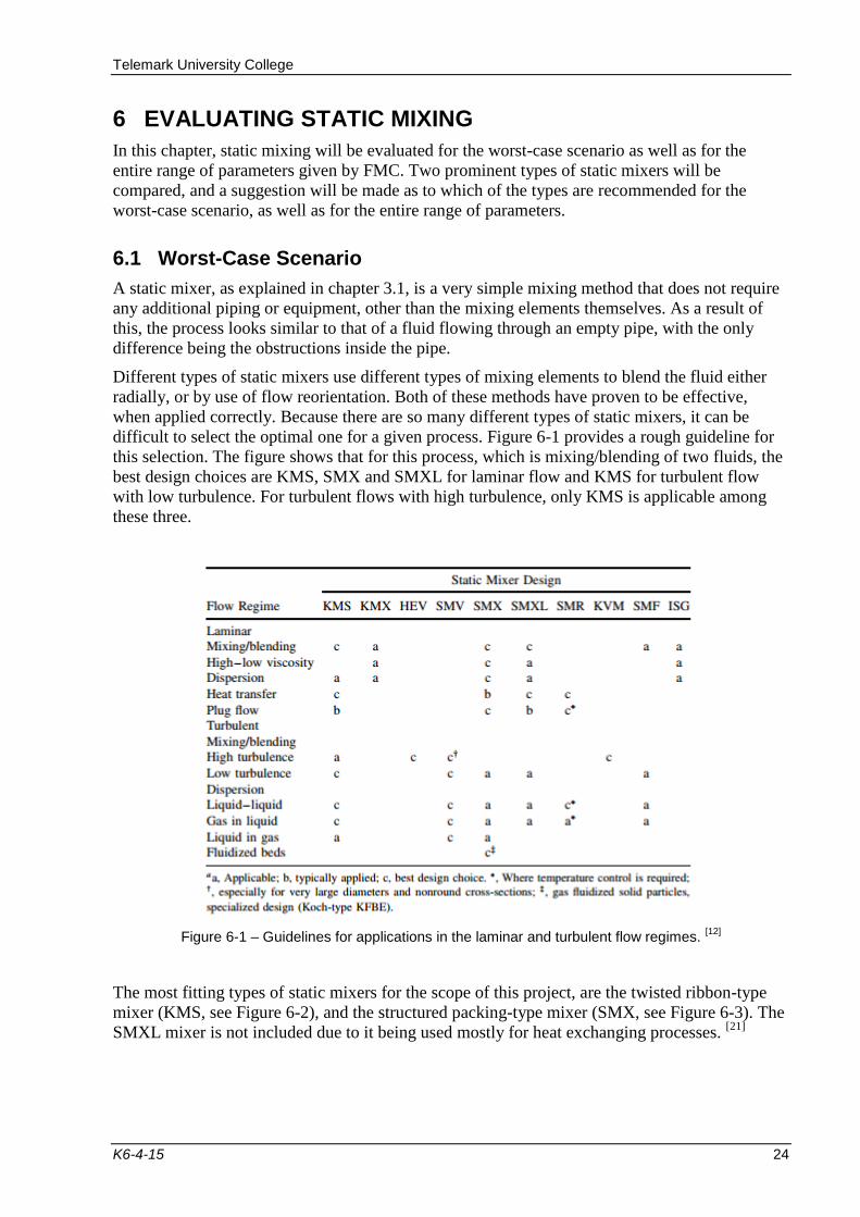
difficult to select the optimal one for a given process. Figure 6-1 provides a rough guideline for
this selection. The figure shows that for this process, which is mixing/blending of two fluids, the
best design choices are KMS, SMX and SMXL for laminar flow and KMS for turbulent flow
with low turbulence. For turbulent flows with high turbulence, only KMS is applicable among
these three.
Figure 6-1 – Guidelines for applications in the laminar and turbulent flow regimes. [12]
The most fitting types of static mixers for the scope of this project, are the twisted ribbon-type
mixer (KMS, see Figure 6-2), and the structured packing-type mixer (SMX, see Figure 6-3). The
SMXL mixer is not included due to it being used mostly for heat exchanging processes. [21]

Telemark University College
K6-4-15 25
Figure 6-2: Twisted-ribbon mixer (KMS) [22]
Figure 6-3: Structured packing mixer (SMX) [23]
In order to decide which type of static mixer to use for a process, it is important to look at how
they perform with the given process parameters. A fairly well used way of measuring
performance of static mixers is comparing the pressure drop created by them, assuming that they
both achieve the same level of mixing, as well as the length required to achieve this criteria. [24]
Calculating pressure drop and required mixing length for static mixers requires various
parameters; most importantly, the degree of mixing must be determined. This parameter is
known as the coefficient of variation CoV, and the smaller this value is, the better the quality of
the mixture. A CoV value of 0.05 means that 95 % of the concentration measurements taken
from the pipe will be within 10 % of the mean concentration. [25]
For the calculations preformed for the static mixers, a CoV value of 0.03 is selected. This is to
ensure that a good mixture quality is achieved.
6.1.1 Mixer Orientation
When mixing in a horizontal pipe, a density difference in the two fluids could increase the
mixing length drastically. The reason behind this is that the fluids will separate quicker, as the
heavier of the fluids will sink to the bottom of the pipe. [12]
It is therefore important to look at the Froude number for this process, and determine whether the
mixing should take place in a vertical pipe. For laminar flow, Equation (6.1) provides a criteria
for orientation. For turbulent flow, Equation (6.2) is used.
(6.1)

Telemark University College
K6-4-15 26
(6.2)
For the worst-case scenario, which is in the laminar flow regime, it is clear that the mixer
orientation should be vertical, due to the relation between Froude and Reynolds number being as
low as 0.000154. These calculations do not take into consideration what kind of mixer is being
used, and therefore it does not matter what solution is chosen. The suggested orientation will
always be vertical for these process parameters.
6.1.2 Calculating Mixing Length and Pressure Drop
Equation (6.3) is used to the coefficient of variance, and uses a -factor called mixing rate
coefficient for blending. This coefficient is different for each type of static mixer, and flow
regime, so that KiL is for laminar flow and KiT is for turbulent. Table 6-1 provides an overview
of the different -factors that will be used for the following calculations.
(6.3)
Table 6-1: List of Ki-values used in length-calculations
Device L T
KMS 0.87 0.50
SMX 0.63 0.46
Equation (6.3) is used to formulate Equation (6.4), which is used to calculate the mixing length.
(6.4)
With this information, it is possible to calculate the required mixing length for both types of
static mixers, using the worst-case parameters. The results of these calculations are found in
Table 6-2 below.
Table 6-2: Required mixing length for both types of static mixer.
Device Length Unit
KMS 3.868 m
SMX 1.166 m
With the mixing length calculated, it is possible to calculate the pressure drop created by these
two static mixers. There are many different ways to do this, but it is very common to use the

Telemark University College
K6-4-15 27
pressure drop in an equivalent empty pipe and multiply that by a K-factor, known as the pressure
drop ratio for motionless mixers, as in Equation (6.5). This K-factor, similarly to the -factor, is
also dependent on the flow regime as well as the mixing device. Table 6-3 provides an overview
of the different K-factors used for the KMS and SMX mixers.
Table 6-3: List of K-values used in pressure drop calculations.
Device KL KT
Empty pipe 1 1
KMS 6.9 150
SMX 37.5 500
By looking at these values in accordance to Equation (6.5), it is obvious that the SMX mixer will
create the biggest pressure drop. The equation used for calculating pressure drop, as presented in
Equation (6.6), is as mentioned a combination of the K-factor and the equation for pressure drop
in an empty pipe.
(6.5)
(6.6)
The friction factor f used in Equation (6.6) is calculated using Equation (6.7) if the flow is
laminar, and Equation (6.8) if the flow is turbulent.
(6.7)
(6.8)
By using these equations, along with the calculated mixing length and the parameters for the
worst-case scenario, it is possible to calculate the pressure drops from each of the static mixers.
Table 6-4 below shows the results from these calculations.
Table 6-4: Pressure drop created by both types of static mixer.
Device Pressure drop Unit
KMS 542.93 Pa
SMX 889.38 Pa
As predicted, the SMX mixer provides the highest pressure drop, despite using almost one third
of the length. As such, the suggestion would be to use a structured packing-type mixer for this
process, due to its short mixing length. The pressure difference between the two mixing methods

Telemark University College
K6-4-15 28
(~345 Pa) is negligible. However, it is important to note that if space is no issue when choosing a
static mixer, the twisted ribbon-type might be more suited due to the smaller pressure drop.
6.1.3 Slight Variations in Process Parameters for the Worst-Case Scenario
When the process is ongoing, it is to be expected that some of the parameters can vary slightly.
To ensure that such small variations will not cause any problems, it is important to take these
variations in consideration when preforming calculations.
For this process, only two parameters will have any effect on the performance of the mixer, these
being the velocity and viscosity of the mixture. The diameter of the pipe is not included for
obvious reasons, and the density and water cut does not affect the calculations of mixing length
or pressure drop for a laminar flow. This can be shown by combining Equation (6.5), (6.6) and
(6.7). The resulting Equation (6.9) shows that only the viscosity and velocity will affect the
pressure drop, when the diameter and resulting mixing length are constant.
(6.9)
It is assumed that the viscosity of the fluid will not increase above the range provided by FMC,
so the only possible variation of this parameter is a decrease, which would result in a reduced
pressure drop. The velocity, on the other hand, could easily decrease to values below the
expected range for various reasons. This is not important due to the resulting decrease in
pressure drop. The only issue that might occur as a result of these variations, is an increase in
velocity because of the increasing pressure drop. Looking at a maximum 20 % increase in
velocity, this would not cause any other issues besides a 20 % increase in pressure drop. This
increase in velocity does not have an effect on the flow regime, as the resulting Reynolds number
would be approximately 166, well below the laminar limit of 2000.
The results of these considerations are that the slight variations in process parameters will not
cause any issues other than a slight increase in pressure drop.
6.2 Varying Parameters
In addition to providing a suggested mixing method for the worst-case scenario, it is also
important to research if the suggested method can work for different parameters within the range
provided by FMC. By varying different parameters and looking at how they affect the
performance of the static mixer, it is possible to fin if there are any limitations regarding the use
of these mixers.
All the parameters listed in the problem description will be varied, starting from the worst case-
value and increasing/decreasing until the entire range is covered. This will first be done
individually parameter by parameter, before all the parameters will be varied simultaneously,
from lowest to highest possible Reynolds number.
6.2.1 Pipe Diameter
From equations used in chapter 6.1, it is clear that an increase in the pipe diameter will result in a
longer mixing length. Figure 6-4 is made using Equation (6.4) with 20 different diameters,
increasing from 0.536 m to 0.768 m.

Telemark University College
K6-4-15 29
Figure 6-4: Mixing length as a function of pipe diameter.
Figure 6-4 gives a clear representation of a problem that arises when the pipe diameter becomes
too large. Due to the mixer orientation being vertical, a very long mixing length can become
problematic because of the space required.
In addition to having an effect on the mixing length, varying the pipe diameter will also affect
the pressure drop created by each static mixer. To plot this in a graph, the same method was used
as with the mixing length, only using Equation (6.9) instead.
Figure 6-5: Pressure drop as a function of pipe diameter.
As Figure 6-5 shows, the pressure drop will decrease with increasing pipe diameter. Despite the
increase in length, the increasing diameter will still result in a smaller pressure drop created for
both types of mixers.
0
5
10
15
20
25
Mix
ing length
[m
]
Pipe diameter [m]
SMX
KMS
0
100
200
300
400
500
600
700
800
900
1000
Pre
ssure
dro
p [P
a]
Pipe diameter [m]
SMX
KMS
Telemark University College
K6-4-15 30
The only problem that occurs when looking at increasing diameter is the length of the mixer. If
there is limited space, these static mixers might become unsuitable if the pipe diameter is too
large.
6.2.2 Density and Water Cut
Looking at Equation (6.9), it is clear that density has no effect on the pressure drop. Nor does it
have any effect on the length of the mixer. When looking at varying water cut, it is assumed that
the oil density remains constant, and therefore the only change would be the total density of the
mixture. Therefore, neither the water cut nor the density will affect the pressure drop or mixing
length.
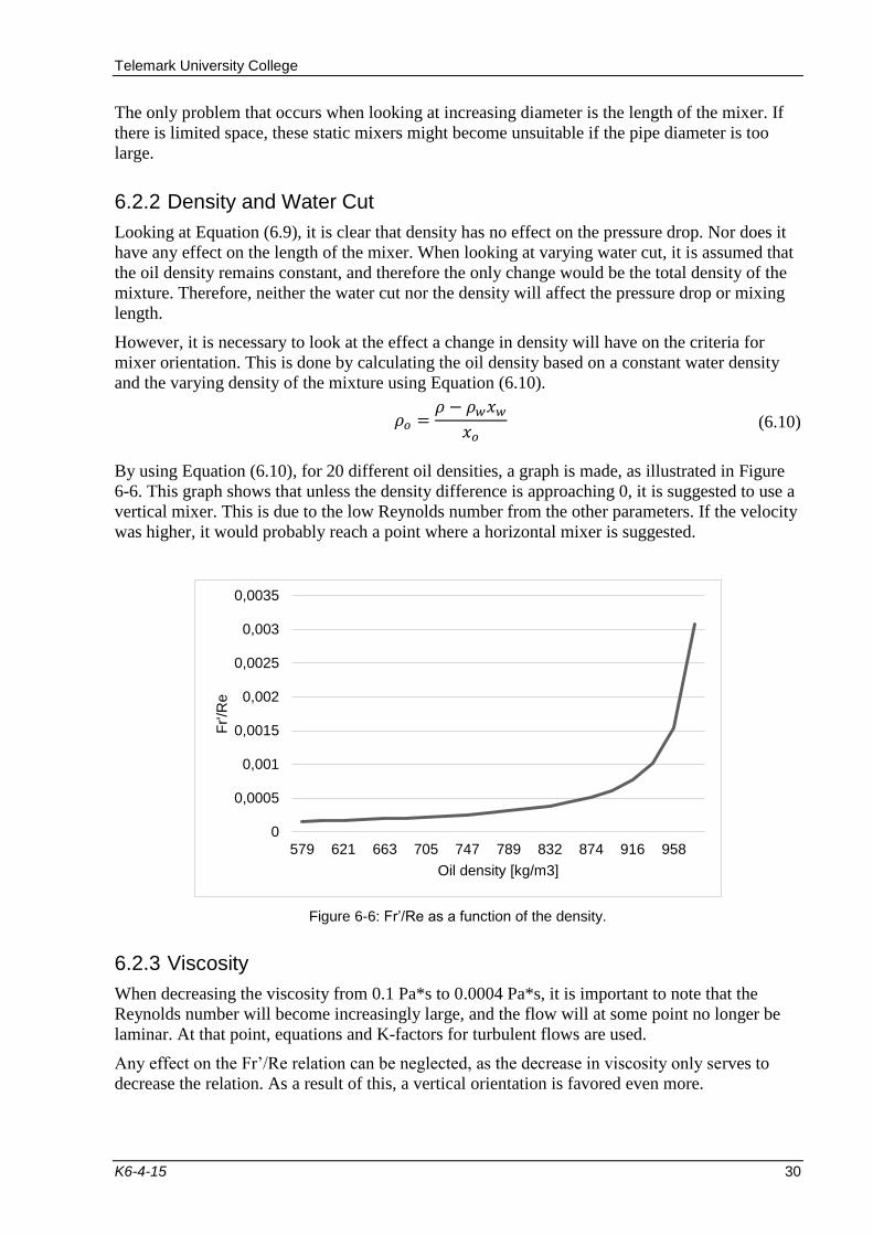
However, it is necessary to look at the effect a change in density will have on the criteria for
mixer orientation. This is done by calculating the oil density based on a constant water density
and the varying density of the mixture using Equation (6.10).
(6.10)
By using Equation (6.10), for 20 different oil densities, a graph is made, as illustrated in Figure
6-6. This graph shows that unless the density difference is approaching 0, it is suggested to use a
vertical mixer. This is due to the low Reynolds number from the other parameters. If the velocity
was higher, it would probably reach a point where a horizontal mixer is suggested.
Figure 6-6: Fr’/Re as a function of the density.
6.2.3 Viscosity
When decreasing the viscosity from 0.1 Pa*s to 0.0004 Pa*s, it is important to note that the
Reynolds number will become increasingly large, and the flow will at some point no longer be
laminar. At that point, equations and K-factors for turbulent flows are used.
Any effect on the Fr’/Re relation can be neglected, as the decrease in viscosity only serves to
decrease the relation. As a result of this, a vertical orientation is favored even more.
0
0,0005
0,001
0,0015
0,002
0,0025
0,003
0,0035
579 621 663 705 747 789 832 874 916 958
Fr'/R
e
Oil density [kg/m3]

Telemark University College
K6-4-15 31
The only effect of a change in viscosity is a decrease in pressure drop, as Equation (6.9)
suggests. However, as previously stated, it is important to note that when the flow leaves the
laminar regime, it could have large effects on the calculations. This is shown in Figure 6-7,
where the pressure drop is decreasing with decreasing viscosity, until the flow becomes turbulent
and different equations are used. Due to the very high KT factor of the SMX-type mixer, the
pressure drop will increase in a much larger rate than for the KMS in the turbulent regime.
The pressure drops for the turbulent flow still remain below those of the values in the worst-case
scenario, so mixing fluids with a viscosity as low as 0.0004 Pa*s should not be problematic.
Figure 6-7: Pressure drop as a function of viscosity
6.2.4 Velocity
Looking at the ranges of parameters from FMC, it is clear that apart from the viscosity, none of
the parameters see such a large percentage increase from minimum to maximum as the velocity.
Seeing also that the values are so much higher than those of the viscosity, it is possible to assume
that a change in velocity will result in large effects on the pressure drop, and the Reynolds
number.
When increasing the velocity from 0.15 to 15.43 m/s, the Reynolds number increases from
138.24 to 12812, and the flow becomes turbulent early on. As Figure 6-8 shows, this has a large
effect on the pressure drops, as they increase to up to ~39 bar for the SMX-type, and ~13 bar for
the KMS-type.
0
100
200
300
400
500
600
700
800
900
1000
Pre
ssure
dro
p [P
a]
Viscosity [Pas]
SMX
KMS

Telemark University College
K6-4-15 32
Figure 6-8: Pressure drop as a function of the velocity
As mentioned in chapter 6.2.3, an increase in velocity could also affect the mixer orientation.
Using the criteria mentioned in chapter 6.1.1 with increasing velocities, it is possible to make
two graphs. One for each flow regime that shows at what point a horizontal mixer orientation can
be considered.
Figure 6-9: Mixer orientation criteria for laminar flow with increasing velocity.
0
500000
1000000
1500000
2000000
2500000
3000000
3500000
4000000
4500000
Pre
ssure
dro
p [P
a]
Velocity [m/s]
SMX
KMS
0
0,0002
0,0004
0,0006
0,0008
0,001
0,0012
0,0014
0,0016
0,0018
0,002
0,15 0,914 1,678
Fr'/R
e
Velocity [m/s]

Telemark University College
K6-4-15 33
Figure 6-10: Mixer orientation for laminar flow with increasing velocity
For laminar flow velocities, it is clear from Figure 6-9 that the mixing orientation should remain
vertical. Looking at Figure 6-10, it clearly shows that when the velocities become larger than
~4.5 m/s, a horizontal mixer is suggested.
6.2.5 All Parameters
By looking at all parameters individually, observations have been made as to which parameter
has the greatest impact on the pressure drop and mixing length parameters. The diameter and
velocity have both shown to create problems for the static mixers, in terms of long mixing length
and high pressure drops respectively. In order to see how all these parameters work together, 20
calculations were performed by increasing velocity, density and diameter and decreasing
viscosity with a constant water cut of 5 %. This results in a range from the lowest possible to the
highest possible Reynolds number. The results of these calculations is illustrated in Figure 6-11
below.
Figure 6-11: Pressure drop affected by increasing the Reynolds number.
0
20
40
60
80
100
120
140
160
180
200
Fr'
Velocity [m/s]
Fr'
Criteria
0
500000
1000000
1500000
2000000
2500000
Pre
ssure
dro
p [P
a]
Reynolds number
SMX
KMS

Telemark University College
K6-4-15 34
When comparing these numbers with the ones from the varying velocity, the pressure drop is
lower. This is due to the diameter and viscosity decreasing the pressure drop as they increase and
decrease respectively. The sudden and large decrease in pressure drop at the end is caused by the
viscosity reaching values close to 0, resulting in a large increase in Reynolds number. In
Equation (6.8), the friction factor will become very small when the Reynolds number reaches
high values, resulting in a low pressure drop as shown in the graph above.
The graph presents a problem that gives an explanation for why SMX is not considered
applicable for high turbulence flows. The KMS is applicable, but not usually used as shown in
Figure 6-1. The pressure drops becomes high when the flow becomes turbulent. It is clear that
the KMS is the better choice for turbulent flows, as Figure 6-1 suggests. On the other hand, the
length of the mixer would still be a problem that would need to be considered.

Telemark University College
K6-4-15 35
7 DESIGN OF A POWER MIXING SYSTEM
In this chapter, a power mixing system will be designed based on the worst-case scenario
parameters presented in chapter 4. All utilities are evaluated to provide a homogeneous flow of
the heterogeneous mixture uploaded to the mixing station. It is taken into account that the
mixture needs to stay homogeneous for a required distance after the mixing station. A high
pressure drop is expensive, and therefore the utilities are evaluated based on the amount of
pressure drop they will add to the process.
7.1 Process Description
The pump needs to compensate for the pressure drop caused by all equipment in the mixing loop.
The size of the pump is measured in head, which is how many meters the pump has to push the
fluid for it to get re-injected and to prevent backflow. Total head needed for the power mixing
can be calculated from Equation (7.1) below.
(7.1)
The size of the pump depends on the pressure, velocity and elevation difference between the
probe and nozzle, as well as the head loss in the mixing loop.
For a power mixing system it is necessary that the pressure out of the mixing nozzle is higher
than in the main pipe. That is why the pump size has to be chosen carefully. The power mix
process is shown in Figure 7-1, where point one and two are marked. Point one is the inlet of the
mixing loop and point two is the outlet.
Figure 7-1: Power-mixing system
The pressure difference is how much pressure that is required in the mixing nozzle to achieve a
homogeneous flow in the main line. Since the pressure in the take-of probe is the same as the
pressure in the main pipe the difference will be the required energy in the mixing nozzle.
The velocity in the mixing loop will be constant because the areal in the pipeline will stay
unchanged throughout the whole power mixer. This can be proven by Equation (7.2) below.
When the difference in velocity is 0, the velocity link in Equation (7.1) can be removed from the
equation. It means that it can be simplified to Equation (7.3).
(7.2)

Telemark University College
K6-4-15 36
(7.3)
When deciding the elevation difference, the distance between the mixing nozzle and sample
probe is evaluated. The mixing system is recommended to be placed in a vertical pipe because it
is easier to achieve good mixing, for reasons explained in chapter 3.2.
Because the mixing system will be placed in a vertical pipe, the elevation difference of the probe
and nozzle will cause a pressure drop. As described in chapter 5, the distance between the
mixing nozzle and sample probe has to be eight pipe diameters. The distance between the mixing
nozzle and the take-off probe to the power mixing loop is suggested to be six times the inner
pipe diameter of the main pipe. This is because it has to be shorter than the distance between the
mixing nozzle and sample probe. The elevation difference can be calculated from Equation (7.4).
(7.4)
Table 7-1: Elevation difference between nozzle and probe
Parameter Value Unit
ΔZ 0.9216 m
The last parameter that needs to be decided before the head of the pump can be calculated is the
head loss through the power-mixing loop. The head loss of the loop is created by elements such
as probe, valves, elbows, filter and tubing. Each different element has its own minor loss
coefficient, which affects the pressure drop through it.
7.2 Utilities
In this chapter, recommendations will be made as to which elements should be used in the power
mixing loop.
7.2.1 Probe
The probe’s function is to extract a portion of the flow in the main pipe that is going to be re-
injected. It is formed as a tube with a bend which will be inserted into the pipeline. To achieve
good mixing, the re-injected flow should be a homogeneous mixture, and therefore the probe has
to be placed within the range where water droplets are uniformly distributed. [20]
The design of the probe is based on the volume flow in the main pipeline. By recycling 10 % of
this flow, a volume flow in the recycle loop can be calculated. For design reasons, the velocity in
the recycle loop is chosen. The area and diameter of the probe, and thereby the recycle pipe, can
be calculated according to Equation (7.5) and (7.6).
(7.5)
√
(7.6)
The parameters are listed in Table 7-2, and the results in Table 7-3.

Telemark University College
K6-4-15 37
Table 7-2: Dimensions of probe and recycle pipe
Symbol Value Unit
Q 0.00027 m3/s
v 0.5 m/s
Table 7-3: Resulting dimensions of the probe.
Symbol Value Unit
Apm 0.00055 m2
di 0.026 m
Regarding the length of the mixing probe into the main pipe, the same limitations due to
vibrations as mentioned in chapter 5.1.2 apply. By assuming a thickness of the probe to be 10
mm, to calculate outside diameter of the probe, the allowable length can now be calculated by
using Equation (5.2). The parameters are listed in Table 7-4 and the result in Table 7-5.
Table 7-4: Parameters and values for the calculations of probe length.
Symbol Value Unit
d0 0.0366 m
di 0.0266 m
V 0.15 m/s
E 1.8822*1011
Pa
600
kg/m3
Table 7-5: Allowable length for the probe.
Symbol Value Unit
L 10 m
Because vortex shedding is increasing proportionally to velocity, and the worst case scenario is
based on a low velocity, there will be no limit of the length in this case. The only restriction is
thereby to avoid placement close to the walls because of the wall effects. The probe should be
placed so that the recycled stream is homogeneous, which is most likely to occur within the area
illustrated in Figure 5-5.
7.2.2 Nozzle
Most of the information and equations are from the international standard 3171. [1]

Telemark University College
K6-4-15 38
A nozzle is a device that can be used to modify the flow of a fluid. In this case, the nozzle is
designed to mix the water into the oil in the flow of the main pipe, by increasing the kinetic
energy at the expense of its pressure. Therefore, the nozzle is one of the most important elements
in the power mixing system. It is formed as a circular tube, of equal diameter as the probe, and
its length having the same limitations as the probe. In the power mixing system, the nozzle’s
main function is to re-inject the recycled portion of the fluid into the main flow, and thereby
achieve a mixed fluid and a homogeneous flow. [26]
To what degree the water droplets are mixed into the crude oil depends on the rate of energy
dissipation. As a result, the nozzle can be designed based on the required energy dissipation. [1][20]
A good dispersion is defined as when the ratio of C1/C2 is between 0.9 and 1. A ratio below 0.4
gives a poor distribution of water droplets, and results in a high potential for water stratification.
(
)
(7.7)
The rate of energy dissipation is calculated by the turbulence characteristics according to
Equation (7.8). The parameters are chosen based on a worst case scenario.
(7.8)
The settling rate of water droplets are thereby calculated by Equation (7.9).
(7.9)
Where G is a parameter dependent on the required ratio of C1/C2. With this, the required energy
for an acceptable concentration profile is determined by Equation (7.10).
(
)
(7.10)
When the required energy for representative sampling is known, the required pressure drop can
be calculated from Equation (7.11).
(7.11)
Bernoulli’s equation, Equation (7.12), can be rearranged to calculate the required velocity of the
re-injection from the nozzle.
(7.12)
The density is not changing, and can be neglected from the equation. The velocity in the main
pipeline will be of such small proportion compared to the re-injection velocity, therefore this too
can be neglected. By rearranging Equation (7.13), the velocity can be calculated as in Equation
(7.14).
(7.13)

Telemark University College
K6-4-15 39
√
(7.14)
When the velocity is known, the re-injection area and diameter can be calculated by Equation
(7.15) and (7.16) respectively, derived from and the continuity Equation (7.2). The parameters
for the calculations are listed in Table 7-6, and the results in Table 7-7.
(7.15)
√
(7.16)
Table 7-6: Parameters for the nozzle design
Symbol Value Unit
166.667 mm2/s
0.00287 m/s
G 10 Dimensionless
W 0.000287 m/s
1000 kg/m3
o 578.947 kg/m3
Er 9.95 W/kg
X 10*D m
Table 7-7: Results for the nozzle design
Symbol Value Unit
P 0.59 bar
vre 14.025 m/s
dre 0.005 m
The re-injection is happening through an outlet of the nozzle, and the degree of mixing is
dependent of the diameter, the amount and the positions of the outlets, as well as the velocity and
angle of re-injections.
In order to determine the most efficient design of the nozzle, simulations needs to be performed.
Some suggestions are as follows:
Re-inject countercurrent to the main flow to provide the most disturbance to the flow.

Telemark University College
K6-4-15 40
Divide the total outlet area into multiple outlets to provide disturbance to a large as
possible portion of the main flow.
Study the effect of varying angles of the outlets.
7.2.3 Pump
In this chapter, the information is found in reference [28].
A pump is a device used to transport fluids through a pipeline. Pumps can be used to move fluids
from a low pressure- to high pressure area, or from a low elevation to a higher elevation. The
types of pumps are divided by how they move the fluid through the pipeline. The four major
types of pumps are: centrifugal-, displacement-, rotary displacement- and Eductor-jet pumps.
Almost every type of pump can be used for gasses and liquids but they will be specially designed
for what type of fluid they are transporting.
When selecting the right pump for the power mixer, it is important to be aware of the ranges in
parameters for this process. There are a lot of different pump types within the four major groups.
The Eductor-jet pump was excluded immediately because the main purpose of this pump was to
mix the process fluid with water, air or steam.
There are many different types of rotary displacement pumps, some of them are only suited for
liquids with high viscosities. Because the ranges in viscosity for the crude oil contains both high
and low values, this type of pump is excluded. The other types of rotary displacement pumps that
were suited for all viscosities had limits for pressure and volume flow. These types can only be
used for processes with pressure between 10 and 40 barg and a volume flow below 60 m3/h, and
as a result of this they are not suited for this process either.
Another option is displacement pumps, but these are more suited for acids and bases.
For petrochemical and oil refinery plants, centrifugal pumps are recommended. This is also the
only type of pump that meets all the criteria for the worst case scenario and the ranges of
parameters.
7.2.4 Valves
The type of valves used for a specific process depends on the pump choice. For this process the
centrifugal pump was recommended, and therefore it is necessary to install two gate valves. One
gate valve has to be placed on the suction side of the pump and the other one is placed on the
discharge side to provide a tight shut off if necessary.
A gate valve gives a low pressure drop, as they offer no resistance to the fluid passing through.
The minor loss coefficient for gate valves is listed in table Table 7-8.
Table 7-8: Minor loss coefficient K for a gate valve. [27]
Type of valve K
Gate Valve, fully open 0.15
To calculate the head loss through a gate valve, Equation (7.17) is used. This mixing loop
contains two gate valves, therefore the head loss has to be multiplied by two.

Telemark University College
K6-4-15 41
(7.17)
To calculate the total pressure drop through these two valves Equation (7.18) is used.
(7.18)
The head loss and pressure drop through the two gate valves for the power mixing are listed in
Table 7-9.
Table 7-9: Results of the head loss and pressure drop for two gate valves in the power mixer system.
Parameter Value Unit
hL 0.0038 m
ΔP 0.0021 bar
7.2.5 Elbows
When selecting the type of elbows for the power mixer the value for the pressure drop is
essential. To keep the pressure drop as low as possible, a 90° long radius elbow is suggested
instead of the 90° regular radius elbow. The difference between these two types, in addition to
the significantly larger pressure drop in the regular radius, is the length and curvature. In a long
radius elbow the radius of curvature is 1.5 times the nominal diameter, while it is one times the
nominal diameter for the regular elbow. Long radius elbows are the most common type of elbow
and are used when the space is available and when the flow is more critical. [29][30]
Threaded and flanged fittings are the two types of fittings for the different sorts of elbows. The
flanged types of elbows cause the least pressure drop. This is because the elbow is attached to
the tubing with a plate outside the pipe. The threaded type is when the elbow is connected with a
screw end inside the pipe. This type of fittings causes the inner diameter to decrease, which
causes a higher pressure drop than the flanged type.
For the power mixer, the flanged long radius 90° elbow is suggested. The minor loss coefficient
value for this type of elbow is listed in Table 7-10 below. Equations (7.17) and (7.18) can still be
used for calculating the pressure drop and head loss through the elbows for this process. It is still
necessary to multiply these equations by two because the loop contains two elbows.
Table 7-10: Minor loss coefficient for 90° long radius elbow. [27]
Type of valve K: Minor loss coefficient value
Elbow, Threaded long radius elbow 90° 0.7
7.2.6 Filter
To prevent damage to the centrifugal pump, there is installed a filter in the power mix loop. The
filter is used to prevent solids from entering the pump because most pumps are not designed to
handle foreign material. A common problem is milling inside the pipes, which is when particles
from the pipe surface detaches and get mixed with the oil. [31][32]

Telemark University College
K6-4-15 42
Mesh is the scale used to determine the opening size in the filter. A common mistake is to use a
too small opening size for the process, which causes the pressure drop to increase dramatically.
For oil, the size of the filter can be 40 mesh or lower depending on the viscosity of the oil. This
means that there are 40 small squares across one inch of screen. 40 mesh has the smallest grids
that is used as filters for oil, and it is guaranteed to remove all particles that might have been
mixed in the oil. Because pressure drop increases with increasing mesh size, it will also cause the
highest possible pressure drop.
To calculate the pressure drop for the necessary filter for this process, the flow coefficient Cv, is
required. The Cv factor can be found in tables when the viscosity of the fluid is known as the
Saybolt Universal viscosity. When calculating the Saybolt Universal viscosity at a certain
temperature, Equation (7.19) has been used. [33]
( ( )) (7.19)
The Saybolt Universal viscosity at 100° F is listed in Table 7-11.
Table 7-11: Saybolt Universal viscosity at 100°F
Parameter Value Unit
U100°F 463 SSU
The result of the Saybolt Universal viscosity at a temperature of 150° C is listed in Table 7-12.
The calculated viscosity is used to find the flow coefficient factor for the filter.
Table 7-12: Result of the Saybolt Universal viscosity at 302° F (150° C)
Parameter Value Unit
U302°F 468 SSU
For a filter that have 40 mesh scale, the Cv value is listed in a table for fluids that have a
viscosity at 30 SSU, 500 SSU and higher viscosities. Due to this, interpolation is required to find
the flow coefficient for the oil that has a viscosity at 468 SSU. Using Equation (7.20) and the
values in Table 7-13, interpolation can be performed.
Table 7-13: Parameters needed for interpolation when calculating the flow coefficient for oil with a viscosity of 468 SSU at 40 Mesh.
[33]
Parameter Value Unit
U1 30 SSU
U2 500 SSU
Telemark University College
K6-4-15 43
Cv1 1.2 Dimensionless
Cv2 1.9 Dimensionless
( )
(7.20)
In Table 7-14, the flow coefficient factor for the oil in the power mixer is listed with a 40 mesh.
Table 7-14: Result of the flow coefficient, Cv, at 302° F (150° C)
Parameter Value Unit
Cv (150° C) 1.85 Dimensionless
To calculate the pressure drop through the filter, Equation (7.21) is used. [34]
(
)
( )
(7.21)
The pressure drop through the filter in the power mix loop is listed in Table 7-15, and is
calculated from the worst-case scenario parameters given in chapter 4.
Table 7-15: Result of the pressure drop in the filter by using the worst-case scenario parameters.
Parameter Value Unit
ΔP 0.39 bar
7.2.7 Piping
When choosing the type of material for the mixing loop, reference [35] and [36] is mostly used.
When deciding the material for the piping in the power mixer, the corrosion resistance, pressure
rating and operating temperature have been taken into consideration. For pipes in oil and gas
production and processing, 22Cr duplex, 6Mo and 316 are different materials that are
recommended.
For the power mixer the 316 stainless steel type of material is suggested. The 316 SS has a high
corrosion resistance and a high strength at elevated temperatures. This material is common for
oil, gas and chemical industries because of its cost and it being easy to fabricate.
The 316 stainless steel material has an L grade, which will reduce the tendency to crack after
welding. For the power mix loop the 316 L is suggested to give an opportunity for welding if it is
necessary.
The length of the tubing in the mixing loop is designed from the international standard 3171. The
distance between the mixing nozzle and the sample probe is recommended to be between one-

Telemark University College
K6-4-15 44
half of the main pipe diameter and eight pipe diameters. Because the probe for the mixing system
has to be before the sampling probe, it is suggested to be placed at six pipe diameters from the
mixing nozzle. The length of vertical pipes is calculated from Equation (7.22). [1]
(7.22)
For design reasons, the length of horizontal piping is suggested to be the same length as the
vertical piping. The length has to be multiplied by two because of the inlet- and outlet pipe. To
calculate the total length of horizontal piping Equation (7.23) has been used.
(7.23)
For total length of tubing in the power mixer, Equation (7.24) has been used.
(7.24)
The total length of tubing for the power mixing system is listed in Table 7-16.
Table 7-16: Results of vertical, horizontal and total tubing in the mixing loop.
Parameter Value Unit
LV 0.9216 m
LH 1.8432 m
Lpm 2.7648 m
The total pipe length is used to calculate the pressure drop caused by friction from the surface
inside the pipe. Equation (7.25) is used to calculate the head loss caused by the tubing in the
mixing loop.
(7.25)
The total head loss caused by the inside surface of the pipe is listed in Table 7-17 below.
Table 7-17: Results of head loss caused by the inside surface of the pipe.
Parameter Value Unit
HL 1.0618 m
To calculate the pressure drop caused by the tubing in the process, Equation (7.21) was used.
The total pressure drop from the pipes in the mixing loop is listed in Table 7-18.

Telemark University College
K6-4-15 45
Table 7-18: Pressure drop in the mixing loop caused by the tubing.
Parameter Value Unit
ΔP 0.0625 Bar
7.2.8 Sizing the Pump
When the pressure difference and the elevation difference between the probe and nozzle, as well
as the head loss through the whole mixing loop is known, the size of the pump can be calculated.
The total head loss for the mixing system can be calculated from Equation (7.26) for the
suggested equipment.
(7.26)
The total head loss through the power mixing system is listed in Table 7-19.
Table 7-19: Total head loss in the power mixer
Parameter Value Unit
hL 7.706 m
The head loss value is further used to calculate the size of the pump. When calculating the head
needed by the pump, Equation (7.27) is used.
(7.27)
Total head needed from the pump in the power mixer is listed in Table 7-20.
Table 7-20: Total head needed from the pump in the power mixer
Parameter Value Unit
hA 18.652 m
To calculate the size of the pump, Equation (7.28) can be used. The pump efficiency is usually
80%, and this is also used for the centrifugal pump for the power mixer.
(7.28)
The size of the pump is listed in Table 7-21. To be sure that the pump will be able to provide the
required energy when varying the velocity in the main pipe, it is also designed for a 20 %
increase of the velocity.
Table 7-21: Pump size for worst case parameters and for a 20 percent increase of the velocity.

Telemark University College
K6-4-15 46
Parameter Value Unit
P 38.12 W
Pdesign 44.68 W

Telemark University College
K6-4-15 47
8 EVALUATING POWER MIXING
In this chapter the power mixing design will be evaluated, and how varying the parameters
throughout the given range will affect the efficiency.
8.1 Worst Case Scenario
The power mixing system described in chapter 7 is based on the worst case scenario, which
parameters are presented in chapter 4. Figure 8-1 below illustrates the designed power mixing
system, including all utilities and dimensions of piping. The equipment labels in this figure are
explained in Table 8-1.
Figure 8-1: Illustration of the designed power mixing system

Telemark University College
K6-4-15 48
Table 8-1: Identifications of items in Figure 8-1.
Label Identification
N-101 Nozzle
V-101 Gate valve
V-102 Gate valve
F-101 Filter
P-101 Pump
I-101 Mixing probe
I-102 Sampling probe
The three main utilities in the power mixing system are the pump, nozzle and probe. In designing
the system, the parameters of the worst case scenario were central. Therefore, the system will
work in its most efficient way when these parameters are the case.
The pump was designed based on the total head loss through the process, the probe design based
on 10% recycle of the main flow, and the nozzle designed to provide the necessary rate of energy
dissipation to the flow. The design will provide a good mix as a homogeneous flow with
parameters varying of 20 %. In this way, it is taken into account that any sudden variations will
not lead to unrepresentative sampling.
The limitations of the system are essential when evaluating if this mixing method will provide a
homogeneous flow for a given process. When designing the nozzle based on the required energy
dissipation, the density of oil and water are crucial, represented by Equation (7.10).
The distance of which the main flow is kept homogeneous after the nozzle, X, has to be
determined by simulation. This parameter was estimated to be maximum ten times the inner
main pipe diameter, as stated in international standard 3171. [1]
8.2 Varying Parameters
8.2.1 Pipe Diameter
The power mixing system is designed for the diameter of the lowest value in the given range of
parameters. Because of this, the designed power mixing system has limitations according to
increasing diameter. The Figure 8-2 below illustrates the required pressure drop in the nozzle
which increases with increasing diameter.

Telemark University College
K6-4-15 49
Figure 8-2: Diameter versus required energy
The mixture is well mixed if the ratio of concentration at the top and bottom are 0.9 or higher,
which gives a G value of ten. If the requirement are lowered to a G value of eight, which is
associated with a concentration ratio of 0.88, the flow will still be homogeneous but maybe not
for as long of a distance as the previous case. On the other hand, when the recycle- and
sampling- probe was placed, there was taken into account that some variations could occur, and
therefore the design distance was less than the maximum allowed distance from the mixing
station. On these grounds, the maximum allowed pressure drop for guaranteed well mixed flow
is higher than the design pressure.
Calculations show that for an increasing diameter, the required pressure drop in the nozzle is
increasing, the pressure drop associated with the piping decreases, and the remaining utilities are
unaffected. The maximum pressure drop that the designed mixing system can handle is
calculated to be 0.87 bar, which correspond to a main pipe diameter of 0.2 m.
If the total pressure drop is considered, the main limiting factor is the pressure drop caused by
the filter. Although there is a maximum allowed pressure drop that the pump can maintain,
simple modifications can be made so that the power mixing system will provide a homogeneous
flow. Figure 8-3 illustrates how the total pressure drop is affected by variations in diameter.
9,9
10,4
10,9
11,4
11,9
12,4
12,9
0,15 0,25 0,35 0,45 0,55 0,65 0,75
Required e
nerg
y [W
/kg]
Diameter [m]

Telemark University College
K6-4-15 50
Figure 8-3: Diameter versus total pressure drop
When the limit of maximum pressure drop is reached, the filter can be changed to one that does
not cause as much pressure drop as the filter chosen for this design, so that the pump can provide
the required effect. Another option is to install a new pump, as the head needed from the pump
increases with increasing diameter. Figure 8-4 shows the required effect versus the pressure
drop.
Figure 8-4: Total pressure drop versus required power from pump
By these grounds, it could be possible to evaluate what option would be the most economical;
changing the filter and keep the pump, or install a new pump which can account for the total
pressure drop as illustrated in the figure above.
0
50
100
150
200
250
300
350
400
450
0,15 0,25 0,35 0,45 0,55 0,65 0,75 0,85
P
[bar]
Diameter [m]
0
50000
100000
150000
200000
250000
300000
350000
400000
450000
500000
0 100 200 300 400 500
Pow
er
[W]
P [bar]

Telemark University College
K6-4-15 51
8.2.2 Velocity
When the velocity increases and all the other parameters remain constant, the volume flow
increases stated by Equation (8.1).
(8.1)
To ensure that the power mixing system will provide a homogeneous flow for realistic velocity
variations, the pump is designed to maintain the pressure drop at ± 20 % variations. The limiting
factor in this case is the pressure drop caused by the filter, which increases with increasing
velocity. Consequently, the head needed from the pump is determined for a flow of velocity of
20 % more than the design velocity.
The required energy and pressure drop in the nozzle decreases with increasing velocity and
volume flow, according to Equation (7.10) and (7.11). Theoretically, the power mixing system
will be functional at velocities from the worst case of a minimum value of 0.15 m/s to 1 m/s.
After this point, the required diameter of the probe and nozzle will increase to a value that is
unrealistic compared to the pipe diameter of 0.1536 m. A velocity of 1 m/s accounts for a
velocity that is six times the design velocity, and an escalation of this extent are unlikely to occur
under normal conditions.
For the case where the velocity is less than the worst case scenario, which can happen if there is
an irregularity to the uploading process, the flow will not be well mixed. It has to be taken into
account that representative sampling cannot be performed under these circumstances.
8.2.3 Density
As the total density increases, the density of oil will increase accordingly because the density of
water is constant. As Figure 8-5 illustrates, the required energy dissipation decreases with
increasing density.
Figure 8-5: Density versus required energy
0
1
2
3
4
5
6
7
8
9
10
600 700 800 900 1000
Required e
nerg
y [
W/k
g]
Density [kg/m3]

Telemark University College
K6-4-15 52
This can be explained by the fact that if the density of oil increases, the difference in density
would decrease. When this occurs, the force of gravity, that has a higher impact the heavier fluid,
will decrease accordingly. Thereby, it can be concluded that the lower the density difference of
oil and water, the mixing becomes less energy consuming. This is illustrated in Figure 8-6.
Figure 8-6: Density difference versus required energy
The graph shows that for no difference in density between water and oil, no energy dissipation is
required. This is according to the calculations, but could be a case where the equations are not
accurate.
In the worst case scenario, the water cut is set to be the highest value in the given range. Because
the density of oil and water are constant for a given flow, a variation on water cut would affect
the total density of the homogeneous mix. Water has the highest density, and therefore, when the
amount of water in the mix increases, the easier the stratification will occur. In Figure 8-7 an
increase of the water cut through the whole given range is illustrated. Because of the force of
gravity, the required energy dissipation increases proportionally with an increasing water cut.
0
1
2
3
4
5
6
7
8
9
10
0 100 200 300 400 500
Required e
nerg
y [
W/k
g]
Density difference [kg/m3]

Telemark University College
K6-4-15 53
Figure 8-7: Water cut versus required energy.
8.2.4 Viscosity
When the viscosity decreases, the Reynolds number will increase. The graph in Figure 8-8 shows
that the required energy dissipation is reduced, as stated in Equation (7.10). The value decreases
as the kinematic viscosity increases, which occurs when the dynamic viscosity increases,
according to Equation (8.2).
(8.2)
This case states the opposite as all the other cases in this chapter; an increase in required energy
when the turbulence in the flow increases.
Figure 8-8: Viscosity versus required energy
8,55
8,65
8,75
8,85
8,95
9,05
0,5 1 1,5 2 2,5 3 3,5 4 4,5 5
Required e
nerg
y [
W/k
g]
Water cut [%]
0
100
200
300
400
500
600
700
0 0,02 0,04 0,06 0,08 0,1
Required e
nerg
y [
W/k
g]
Viscosity [Pa*s]

Telemark University College
K6-4-15 54
8.2.5 All Parameters
As explained in chapter 4, the worst case scenario is set to be when we have the minimum
Reynolds number. According to Equation (4.1), this number will increase when the density,
velocity and diameter increases, and the viscosity decreases.
When evaluating an increasing Reynolds number, which is equivalent to an increasing
turbulence in the flow, the parameters are varied through the given range.
Figure 8-9: Reynolds number versus pressure drop
The graph in Figure 8-9 shows that for increasing turbulence in the main flow, the lower the
pressure drop, because of a lower required energy dissipation for providing satisfying mixing.
This can be explained by the fact that to achieve a turbulent flow, energy is added, and this
energy has provided some mixing before the main flow reaches the mixing station. In other
words, energy required from the power mixing system decreases when the turbulence already
present in the flow increases.
0
100
200
300
400
500
600
0 10000 20000 30000 40000 50000
Pre
ssure
dro
p [P
a]
Reynold's number
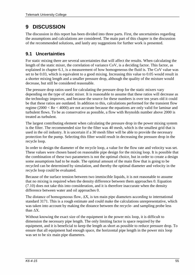
Telemark University College
K6-4-15 55
9 DISCUSSION
The discussion in this report has been divided into three parts. First, the uncertainties regarding
the assumptions and calculations are considered. The main part of this chapter is the discussion
of the recommended solutions, and lastly any suggestions for further work is presented.
9.1 Uncertainties
For static mixing there are several uncertainties that will affect the results. When calculating the
length of the static mixer, the correlation of variance CoV, is a deciding factor. This factor, as
explained in chapter 6.1, is a measurement of how homogeneous the fluid is. The CoV value was
set to be 0.03, which is equivalent to a good mixing. Increasing this value to 0.05 would result in
a shorter mixing length and a smaller pressure drop, although the quality of the mixture would
decrease, but still be considered reasonable.
The pressure drop ratios used for calculating the pressure drop for the static mixers vary
depending on the type of static mixer. It is reasonable to assume that these ratios will decrease as
the technology improves, and because the source for these numbers is over ten years old it could
be that these ratios are outdated. In addition to this, calculations performed for the transient flow
regime (2000 < Re < 4000) are not accurate because the equations are only valid for laminar and
turbulent flows. To be as conservative as possible, a flow with Reynolds number above 2000 is
treated as turbulent.
The largest contributing element when calculating the pressure drop in the power mixing system
is the filter. The recommended size for the filter was 40 mesh, which is the smallest grid that is
used in the oil industry. It is uncertain if a 30 mesh filter will be able to provide the necessary
protection for the pump. Selecting this filter would result in decreasing the pressure drop in the
recycle loop.
In order to design the diameter of the recycle loop, a value for the flow rate and velocity was set.
These values were chosen based on reasonable pipe design for the mixing loop. It is possible that
the combination of these two parameters is not the optimal choice, but in order to create a design
some assumptions had to be made. The optimal amount of the main flow that is going to be
recycled can be determined by simulation, and thereby the optimal diameter and velocity in the
recycle loop could be evaluated.
Because of the surface tension between two immiscible liquids, it is not reasonable to assume
that no mixing is required when the density difference between them approaches 0. Equation
(7.10) does not take this into consideration, and it is therefore inaccurate when the density
difference between water and oil approaches 0.
The distance of homogeneous flow, ΔX, is ten main pipe diameters according to international
standard 3171. This is a rough estimate and could make the calculations unrepresentative, which
was taken into account by making the distance between the recycle- and sampling probe less
than ΔX.
Without knowing the exact size of the equipment in the power mix loop, it is difficult to
dimension the necessary pipe length. The only limiting factor is space required by the
equipment, and it is beneficial to keep the length as short as possible to reduce pressure drop. To
ensure that all equipment had enough space, the horizontal pipe length in the power mix loop
was set to be six main pipe diameters.

Telemark University College
K6-4-15 56
9.2 Recommended Solutions
The mechanically agitated vessel was excluded due to the high power consumption and because
it is not an efficient in-line mixing system. An in-line design made with turbine impellers and
baffles with two steps will be able to mix the two immiscible liquids. However, the amount of
energy required for mixing in a vessel will be too high compared to the other mixing methods.
A fast loop sampling system is recommended because it prevents valuable oil from going to
waste, and the samples will be of a higher accuracy. CoJetix sampler provides the lowest
uncertainty to the samples, but can only be installed in a power mixer. An intermittent type of
sampler is suggested to be used for extraction of the samples, because it has the ability to vary
the sampling frequency or grab volume in proportion to the flow rate.
The static- and power mixing systems were suggested to be designed in a vertical pipe for the
worst case scenario because it is easier to achieve a good mixture than in a horizontal system.
The gravitational force will not affect the separation of the water and oil as much in a vertical
pipe as in a horizontal pipe.
When comparing static mixers for the worst case scenario, the structured packing type is
recommended even though it has a higher pressure drop than the helical type. When the pipe is
vertical, space quickly becomes an issue, and the structured packing type has a shorter mixing
length than the helical mixer. If space is no issue, helical mixer might be more suited. These
results correlate to other previous studies. [24]
When the Reynolds number reaches values above 2000, the pressure drop created by static
mixers becomes significantly larger because the obstructions cause more resistance to the flow.
When the main pipe diameter increases, the mixing length increases to an extent that will most
likely cause space issues. The limit was set to a pipe diameter of 0.4 m, which correspond to a
mixing length of 3 m for the structured packing mixer. A larger pipe diameter is possible if space
is no issue.
For the probe and nozzle, the dimensions will change accordingly to the diameter of the main
pipe. The pressure drop increases, and thereby the velocity of the re-injection through the nozzle
and the total area of the outlets increases with increasing diameter. The design of the nozzle
should be evaluated so that any modifications that will provide a more sufficient, or simpler,
mixing can be conducted.
The allowed length of probe and nozzle, as mentioned in chapter 7.2.1, will be of a higher value
then the main pipe diameter for all variations of parameters. Because of this, it is possible to
insert these utilities at the preferred or recommended length into the main pipe diameter.
For the case where the density difference decreases, the orientation of the pipe can be discussed.
As the density difference decreases, the force that the gravity exerts on the water decreases, and
at some limit the power mixing can be performed in a horizontal pipe without negligible negative
effect on the degree of mixing.
When varying the different parameters for the mixing loop it is necessary to make some
modifications.
The pump that was recommended for this process was based on the different ranges of the
parameters. When the centrifugal pump was the only type of pump that was able to work for all
the different criteria it can still be used when varying the different parameters. When varying the
parameters that changes the power required to achieve a homogeneous flow, the sizing of the
pump needs modifications. When the required energy increases a larger pump is required and
vice versa.
Telemark University College
K6-4-15 57
The valves for the power mixer was chosen with respect to the pump used for the mixer. One
gate valve installed before and one after the pump to provide a tight shut off. Because the pump
type can remain the same when varying the parameters the valves does not have to be changed
either.
For the power mixer, two 90° flanged long radius elbows were recommended because they
caused the least pressure drop for the process. Flanged elbows can handle more pressure
compared to the threaded type, therefore the pressure increase in the process should not be a
problem. When varying the worst case parameters the elbows will not get affected.
The filter that was recommended for this power mixer will work for the worst case parameters.
When the volume flow increases the pressure drop through the filter will increase significantly.
Parameters that affect the volume flow are the diameter of the pipe and velocity of the fluid. The
pump is designed to handle the pressure drop for this process with a 20 % increase of the
velocity. If the velocity escalates with more than 20 % the pump will not be powerful enough to
maintain the pressure needed.
When comparing static mixing to power mixing in the worst case scenario, there are two
important arguments; pressure drop and costs. Static mixing provides a lower pressure drop as
well as lower capital and operation costs, and is therefore the suggested method. When the
turbulence in the flow increases, the required energy and thereby the pressure drop in the power
mixing loop decreases. Because of this, when the flow is no longer laminar, the pressure drop in
the static mixer will be higher than in the power mixing system, and the power mixer is the
suggested method.
9.3 Suggestions for Further Work
When the flow reaches a Reynolds number high enough that the mixing will happen naturally
has to be determined by simulation. An optimal design of the nozzle and the distance of a
homogeneous flow, X, should to be determined this way as well. In order to confirm or
disprove the conclusions, simulations for different scenarios should be performed.
For the calculations of required energy, variations in viscosity result in unreliable values. The
reason behind this should be studied further.

Telemark University College
K6-4-15 58
10 CONCLUSION
The mechanically agitated vessel is not a recommended mixing system for this process due to
high power consumption. The power- and static mixers are more suited for mixing in pipelines.
For the sampling system, an intermittent sampler is the recommended method for extraction of
samples. It will be installed into a horizontal fast loop with three sampling probes, which will be
placed at the top, bottom and one in the cross section of the pipe where the flow is homogeneous.
The suggested static mixer for the worst case scenario parameters is the structured packing type.
When the diameter becomes too large, this type of mixing becomes difficult because of a large
required mixing length. If the mixing orientation is vertical, a long mixing length could cause
space issues. Another problem area is when the flow leaves the laminar region, as this results in a
high pressure drop.
When designing the power mixing system, choosing type of utilities is essential. A centrifugal
pump is suggested, and it requires two gate valves. A filter has to be installed, and in this case a
40 mesh is recommended. The chosen type elbows for this system is the flanged 90° long radius.
A problem area for the designed power mixing system is when the velocity changes by more
than 20%, because the pressure drop caused by the nozzle or filter increases to a value that the
pump can’t compensate for.
A static mixer is recommended for Reynolds numbers below 2000 and a main pipe diameter
below 0.4 m. The suggested mixing method for a main pipe diameter above 0.4 m and/or
Reynolds Numbers above 2000 is a power mixing system. When the Reynolds number reaches a
certain point, it is reasonable to assume that the flow is naturally mixed by turbulence, and no
further mixing is required. This is illustrated in Figure 10-1.
Figure 10-1: Suggested mixing method for the range of diameters and Reynolds number.

Høgskolen i Telemark Referance
K6-4-15 59
REFERANCE
[1] Petroleum liquids – Automatic pipeline sampling, ISO 3171, 1988
[2] Wikipedia. (2015). Petroleum. Available: 22.03.2015,
http://en.wikipedia.org/wiki/Petroleum
[3] Smithsonian. (2010). Oil and Water Do Mix. Available: 22.03.2015,
http://www.smithsonianmag.com/science-nature/oil-and-water-do-mix-38726068/?no-ist
[4] Wikipedia. (2015). Mixing (process engineering). Available: 24.02.2015,
http://en.wikipedia.org/wiki/Mixing_(process_engineering)
[5] N. Harnby, et al. Mixing in the process industries second edition. London: Butterworth-
Heinemann Ltd, 1992.
[6] StaMixCo. Principle of Operations. Avaliable 15.05.2015:
http://stamixco.com/images/principle-of-operations/schema2.jpg
[7] Journey to Forever. Still Designs. Avaliable 15.05.2015:
http://journeytoforever.org/biofuel_library/ethanol_motherearth/z/fig7-1.jpg ¨
[8] Jiskoot. (2014). Jet Mixing. Available: 22.02.2015,
http://www.jiskoot.com/downloads/TS005-0812-3%20JetMixing.pdf
[9] Jiskoot. (2014). Which Mixer is Best. Available: 26.02.2015,
http://www.jiskoot.com/Teach_Me/Which_mixer_is_best/Which_mixer_is_best.html
[10] Jiskoot. (2014). Comparison of In-line (with JetMix) and static mixing sampling
systems. Available:
20.05.2015:http://jiskoot.com/files/0000/1111/2222/JetMix%20v%20StaticMix-R1.pdf
[11] Jiskoot. (2014). Jet Mixing. Available: 12.05.2015,
http://www.jiskoot.com/downloads/TS005-0812-3%20JetMixing.pdf
[12] E. L. Paul, Handbook of Industrial Mixing. Hoboken, New Jersey: John Wiley & Sons,
Inc., 2004.
[13] J.R. Couper, et al. Chemical Process Equipment. U.S.A: Gulf Professional Publishing,
2012.
[14] University of Babylon. (Year of original upload unknown). Mixing and Agitation of
Fluids. Avaliable: 21.03.2015,
http://www.uobabylon.edu.iq/uobColeges/ad_downloads/5_4863_857.pdf
[15] Jiskoot. (2014). Power point presentation of sampling. Avaliable: 21.03.2015,
http://es.slideshare.net/PaulBagnall/sampling-rev-1-presentation
[16] Steve Watson Gabriel, Meeting with FMC, 12.03.2015
[17] Jiskoot. (2014). Sampling systems – the options. Available: 19.05.2015:
http://www.jiskoot.com/services/sampling/teach-me/sampling-system
[18] T. Marlin. (2013). Onstream Analyzers. Available: 20.04.2015, http://www.pc-
education.mcmaster.ca/Instrumentation/analyzer.htm
[19] T. Walters, Industrial Sampling Systems, U.S.A: Swagelok Company, 2013
[20] Jiskoot. (2014). Fast Loop Sampling. Available: 10.02.2015,
http://www.jiskoot.com/Calculation_System_Solutions/Fast_Loop/index.html

Høgskolen i Telemark Referance
K6-4-15 60
[21] Sulzer Ltd. Multitube Heat Echanger Type SMXLTM
. Available: 13.05.2015,
https://www.sulzer.com/en/Products-and-Services/Agitators-Mixers-and-
Dispensers/Static-Mixers/Heat-Exchangers-and-Reactors/SMXL-Multitube
[22] Chemineer. KM Mixers. Avaliable 15.05.2015:
http://www.chemineer.com/products/kenics/km-mixers.html
[23] StaMixCo. X Grid Static Mixer for Laminar Flow Applications. Avaliable 15.05.2015:
http://stamixco.com/X-Grid-Static-Mixer-laminar-flow-mixing-and-or-dispersion-of-
viscous-fluids
[24] D. Rauline et. al., “A Comparative Assessment of the Performance of the Kenics and
SMX Static Mixers,” Chemical Engineering Research and Design, vol. 78, p. 389-396,
2000.
[25] Statiflo International Ltd. (2015). Coefficient of Variation (CoV). Avaliable 13.05.2015:
http://www.statiflo.com/en/about-static-mixing/mixture-quality/145-coefficient-of-
variation-cov
[26] Wikipedia. (2015). Nozzle. Available: 15.03.2015, http://en.wikipedia.org/wiki/Nozzle
[27] The Engineering Toolbox. (2015). Minor Loss Coefficients in Pipes and Tubes
Components. Available: 12.03.2015, http://www.engineeringtoolbox.com/minor-loss-
coefficients-pipes-d_626.html
[28] E. Ignatowitz. Prosess-kjemi. Norge: Gyldendal Norsk Forlag AS, 2002.
[29] Piping Study. (2015). 90° Elbows. Available: 01.05.2015,
http://www.pipingstudy.com/elbow.html
[30] Marine Sight. (2012). Pipes and Bends – An Essential Guide for Second Engineers: Part
2. Available: 01.05.2015, http://www.marineinsight.com/marine/marine-
news/headline/pipes-and-bends-an-essential-guide-for-second-engineers-part-2/
[31] Pompetravaini. (År). Operating Manual for Centrifugal Pumps. Available: 04.05.2015,
http://www.travaini.nl/Manual/Centrifugaal/ManualeCentrifughe.pdf
[32] F. Evans. (ÅR). Rules to Follow to Avoid Pump Problems. Available: 04.05.2015,
http://www.pumps-filters.com/images/Rules_to_Follow_to_Avoid_Pump_Problems,_2-
16-00.pdf
[33] The Engineering Toolbox. (2015). Viscosity Converting Chart. Available: 05.05.2015,
http://www.engineeringtoolbox.com/viscosity-converter-d_413.html
[34] Eaton Corporation. (2013). Pressure Drop Calculations.
[35] Norsok Standard. (1994). Materials Selection. Available: 07.05.2015,
http://www.standard.no/pagefiles/1174/m-dp-001r1.pdf
[36] Ak Steel. (2007). 316/316L Stainless Steel. Available: 07.05.2015,
http://www.aksteel.com/pdf/markets_products/stainless/austenitic/316_316l_data_sheet.

Høgskolen i Telemark Appendix
K6-4-15 61
APPENDIX
Enclosure A Task from FMC
Enclosure B Historical Data from FMC

Enclosure A – Task from FMC

Bachelor Student’s Project – Power Mixing System

FMC Kongsberg Metering AS
Page no. :3 of 8
Bachelors Student Project
Table of Contents
1 INTRODUCTION ............................................................................ 4
2 CONCEPT ...................................................................................... 5
3 SCOPE OF THE PROJECT ................................................................ 7
4 STANDARDS FOR SAMPLING ........................................................ 8

FMC Kongsberg Metering AS
Page no. :4 of 8
Bachelors Student Project
1 INTRODUCTION
Measurement of oil comprises both quantity and quality. Custody transfer ( or Fiscal measurement ) valuation is based on the "useable" oil so both measures are significant to trade and integrity. Quality is determined by sampling the oil. The oil is sampled to establish the composition quality, density and water content. To evaluate the water content of crude oil requires that the sample shall be fully representative. Representativeness is ensured by good mixing of the oil before sampling is done. Mixing is achieved by the natural turbulence in the pipes or by static mixer or power mixer.

FMC Kongsberg Metering AS
Page no. :5 of 8
Bachelors Student Project
2 CONCEPT
One method of achieving homogeneous flow is called power mixing. Which means mixing is achieved when a portion of the flow is re-introduced into the pipeline via a pump and high-velocity injector. The power mixer system, designed to ensure that the process fluid in the main line is fully homogeneous and ready for sampling. It consists of a take-off ‘Quill’, used to extract a portion of liquid from the mainline, a pump to provide the mixing energy required and a mixing ‘Nozzle’ assembly.
In operation, a proportion of the process fluid is withdrawn from the main pipeline and pumped to the Nozzle assembly. The Mix Nozzle is precision machined with a series of holes so that the fluid is re-injected back into the main pipeline in the form of high velocity jets.
Mixing Nozzle Take off Quill

FMC Kongsberg Metering AS
Page no. :6 of 8
Bachelors Student Project
The Nozzle is inserted into the main pipeline so that these are positioned to ensure that the maximum energy addition is directed to where the water concentration is highest. This is especially advantageous for low flow rates where stratification will occur and free water may flow along the bottom of the pipeline. These jets disperse any transient slugs of water and reduce any large globules of water into small droplets, then distribute these smaller droplets across the pipe cross section. With the Quill positioned in the homogeneous zone downstream of the Nozzle assembly, some of the liquid injected back into the pipeline will be drawn back into the quill and passed through the system again. This recirculation has an averaging effect on any quality transients, which improves the accuracy of intermittent type samplers. As the main line flow rate drops so the percentage of process fluid re-circulated increases. Using a constant pump flow rate, the total rate of energy added to the liquid in the pipeline is constant. Thus, as the flow rate in the pipeline decreases so the energy added per unit of the main line flow increases. As a result the power mixing system copes with an almost infinite flow rate turndown. The Nozzle assembly forms only a small obstruction in the pipeline and the pressure drop caused by it, even at high flow rates, is negligible

FMC Kongsberg Metering AS
Page no. :7 of 8
Bachelors Student Project
3 SCOPE OF THE PROJECT
The scope of project is to develop a power mixing system, including the design of mixing nozzle, sizing of pumps and the sample quill which ensures proper mixing of the oil based on the following Process data:
Parameters which will determines the good mixing can be
1. The flow rate in the pipe line and the flow rate in the sampling branch. 2. The water fraction and the distribution of the water drops in the pipe cross
section upstream the mixing nozzle . 3. The pipe diameter, the diameter of the branch pipe and the diameters of
the holes in the mixing nozzle. 4. The geometry of the mixing nozzle, number of holes and the directions of
the emerging jets. 5. The length of the injector protruding into the pipe line. 6. The length in the pipe line between the mixing nozzle and take off quill. 7. The fluid properties (density, viscosity) for both oil and water. 8. The size of the water drops. 9. The turbulence level in the pipe due to flow and upstream equipment
(pumps, valves).
The size of the pipe line where power mixing system will be applied varies from 8” to 32”. We also welcome any alternative economical solutions which meet mixing requirements.

FMC Kongsberg Metering AS
Page no. :8 of 8
Bachelors Student Project
4 STANDARDS FOR SAMPLING
The following relevant standards are identified: 1. ISO 3171:1988
2. API MPMS Chapter 8.2

Enclosure B – Data from FMC
Screened Range
Target Range (Initial Screening)
Header Size Range (in inches) 6 to 30"
Min Velocity in Header (m/s) 0,15
Density (Kg/m3) 600 to 1000
Viscosity (cP) .4 to 100
Pressure (Bar g) 0 to 100
Temperature (Deg C) 150
Water Cut (%) .5 to 5
Interfacial tension between HC and Water
(typically 25 mN/m) 25

