assessment of pulse tube mixing for vessels … · rheological bound to assess pulse tube mixing...

PNWD-3827 WTP-RPT-155 Rev 0

Assessment of Pulse Tube Mixing for Vessels Containing Non-Newtonian Slurries D. E. Kurath P. A. Meyer J. R. Bontha A. P. Poloski J. A. Fort W. H. Combs W. C. Buchmiller I. D. Welch M. D. Bleich February 2007 Prepared for Bechtel National, Inc. under Contract No. 24590-101-TSA-W000-00004

LEGAL NOTICE This report was prepared by Battelle – Pacific Northwest Division (Battelle) as an account of sponsored research activities. Neither Client nor Battelle nor any person acting on behalf of either: MAKES ANY WARRANTY OR REPRESENTATION, EXPRESS OR IMPLIED, with respect to the accuracy, completeness, or usefulness of the information contained in this report, or that the use of any information, apparatus, process, or composition disclosed in this report may not infringe privately owned rights; or Assumes any liabilities with respect to the use of, or for damages resulting from the use of, any information, apparatus, process, or composition disclosed in this report. References herein to any specific commercial product, process, or service by trade name, trademark, manufacturer, or otherwise, does not necessarily constitute or imply its endorsement, recommendation, or favoring by Battelle. The views and opinions of authors expressed herein do not necessarily state or reflect those of Battelle.

iii

Testing Summary The U.S. Department of Energy (DOE) Office of River Protection’s Waste Treatment Plant (WTP) is being designed and built to pretreat and then vitrify a large portion of the wastes in Hanford’s 177 underground waste storage tanks. The WTP consists of three primary facilities: pretreatment, low-activity waste (LAW) vitrification, and high-level waste (HLW) vitrification. The pretreatment facility receives waste feed from the Hanford tank farms and separates it into 1) a high-volume, low-activity liquid stream stripped of most solids and radionuclides and 2) a much smaller-volume HLW slurry containing most of the solids and most of the radioactivity. Many of the vessels in the pretreatment facility will contain pulse jet mixers (PJMs) that will provide some or all of the mixing in the vessels. This technology was selected for use in so-called “black cell” regions of the WTP where maintenance capability will not be available for the operating life of the WTP. PJM technology was selected because it has no moving mechanical parts that require maintenance. The vessels with the most concentrated slurries will also be mixed with air spargers and/or steady jets in addition to the mixing provided by the PJMs. This report contains the results of pulse tube mixing tests conducted in a half-scale replica of the lag storage vessel constructed in one of the large tanks in the high bay of the Battelle – Pacific Northwest Division (PNWD) 336 Building test facility. The tests used clay with rheological properties at the upper rheological bound to assess pulse tube mixing for vessels containing non-Newtonian slurries. Objectives Table S.1 summarizes the objectives and results of the pulse tube mixing tests.

iv

Table S.1. Summary of Test Objectives and Results(a)

Test Objective Objective Met? Discussion

Determine cavern size during equivalent PJM operations previously tested in the half-scale lag storage vessel

Yes The cavern size was determined using the sodium chloride salt tracer method during operation of the PJMs at half- and full-stroke.

Determine the extent of fluid mixing in the PJM during limiting normal operations

Yes A video camera inserted into pulse tube #7 revealed that the jet generated during refill shifted to the side of the pulse tube opposite the nozzle (inward toward the center of the PJM cluster assembly). The video camera was also used to assess mixing in the pulse tube at a variety of conditions by observing the level of surface agitation. The results of the video cameramonitoring technique are presented in Section 5. Two tracer tests were conducted to evaluate fluid mixing inside a PJM. In one test, tracer was added to the mixing cavern while the pulse tubes were operated at half stroke. Results of this test are presented in Section 5. In the second test, tracer was added to the mixing cavern while pulse tubes operated at full-stroke equivalent. Results are presented in Section 6.

Test Exceptions Table S.2 shows a summary description of the test exceptions applied to the pulse tube mixing tests.

Table S.2. Test Exceptions

Test Exceptions Description of Test Exceptions 24590-WTP-TEF-RT-05-00002 This test exception specified that an interim report be issued with the results of the

pulse tube mixing test and that a final report be issued containing both the controller and instrumentation and the pulse tube mixing test results.

24590-WTP-TEF-RT-05-00003 This test exception specified additional scope for the mixing tests: 1) Using the video monitoring techniques, determine the slurry jet penetration

height during PJM refill as affected by the PJM slurry nozzle velocity. 2) Evaluate the methodology to scale-up the one-half scale PJM mixing data for

full-scale application. 24590-WTP-TEF-RT-06-00001 This test exception specified an additional salt tracer test to determine the

number of full strokes required to fully mix PJM contents with a clay stimulant. 24590-WTP-TEF-RT-06-00002 This test exception specified an additional sampling port to be added to the test

PJM to investigate the possibility of a stagnant zone in the pulse tube. 24590-WTP-TEF-RT-07-00001 This test exception deleted some of the additional scope specified in 24590-

WTP-TEF-RT-05-00003 and specified that the results presented in this document should be published as a separate report, instead of combined with the Controller and Instrumentation testing results.

(a) Test objectives and results associated with Controller and Instrumentation testing as specified in test specification 24590-WTP-TSP-RT-05-002 and Test Plan TP-RPP-WTP-428 Rev. 0, as modified by test exceptions 24590-WTP-TEF-RT-05-00002, 24590-WTP-TEF-RT-05-00003, 24590-WTP-TEF-RT-06-00001, 24590-WTP-TEF-RT-06-00002 and 24590-WTP-TEF-RT-07-00001 are discussed in WTP-RPT-146, Pulse Jet Mixer Controller and Instrumentation Testing.

v

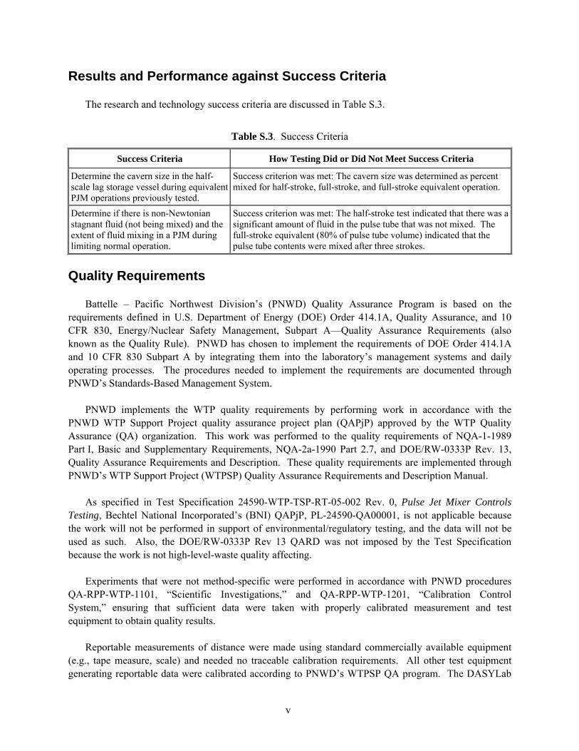
Results and Performance against Success Criteria The research and technology success criteria are discussed in Table S.3.

Table S.3. Success Criteria

Success Criteria How Testing Did or Did Not Meet Success Criteria

Determine the cavern size in the half-scale lag storage vessel during equivalent PJM operations previously tested.

Success criterion was met: The cavern size was determined as percent mixed for half-stroke, full-stroke, and full-stroke equivalent operation.

Determine if there is non-Newtonian stagnant fluid (not being mixed) and the extent of fluid mixing in a PJM during limiting normal operation.

Success criterion was met: The half-stroke test indicated that there was a significant amount of fluid in the pulse tube that was not mixed. The full-stroke equivalent (80% of pulse tube volume) indicated that the pulse tube contents were mixed after three strokes.

Quality Requirements Battelle – Pacific Northwest Division’s (PNWD) Quality Assurance Program is based on the requirements defined in U.S. Department of Energy (DOE) Order 414.1A, Quality Assurance, and 10 CFR 830, Energy/Nuclear Safety Management, Subpart A—Quality Assurance Requirements (also known as the Quality Rule). PNWD has chosen to implement the requirements of DOE Order 414.1A and 10 CFR 830 Subpart A by integrating them into the laboratory’s management systems and daily operating processes. The procedures needed to implement the requirements are documented through PNWD’s Standards-Based Management System. PNWD implements the WTP quality requirements by performing work in accordance with the PNWD WTP Support Project quality assurance project plan (QAPjP) approved by the WTP Quality Assurance (QA) organization. This work was performed to the quality requirements of NQA-1-1989 Part I, Basic and Supplementary Requirements, NQA-2a-1990 Part 2.7, and DOE/RW-0333P Rev. 13, Quality Assurance Requirements and Description. These quality requirements are implemented through PNWD’s WTP Support Project (WTPSP) Quality Assurance Requirements and Description Manual. As specified in Test Specification 24590-WTP-TSP-RT-05-002 Rev. 0, Pulse Jet Mixer Controls Testing, Bechtel National Incorporated’s (BNI) QAPjP, PL-24590-QA00001, is not applicable because the work will not be performed in support of environmental/regulatory testing, and the data will not be used as such. Also, the DOE/RW-0333P Rev 13 QARD was not imposed by the Test Specification because the work is not high-level-waste quality affecting.

Experiments that were not method-specific were performed in accordance with PNWD procedures QA-RPP-WTP-1101, “Scientific Investigations,” and QA-RPP-WTP-1201, “Calibration Control System,” ensuring that sufficient data were taken with properly calibrated measurement and test equipment to obtain quality results. Reportable measurements of distance were made using standard commercially available equipment (e.g., tape measure, scale) and needed no traceable calibration requirements. All other test equipment generating reportable data were calibrated according to PNWD’s WTPSP QA program. The DASYLab

vi

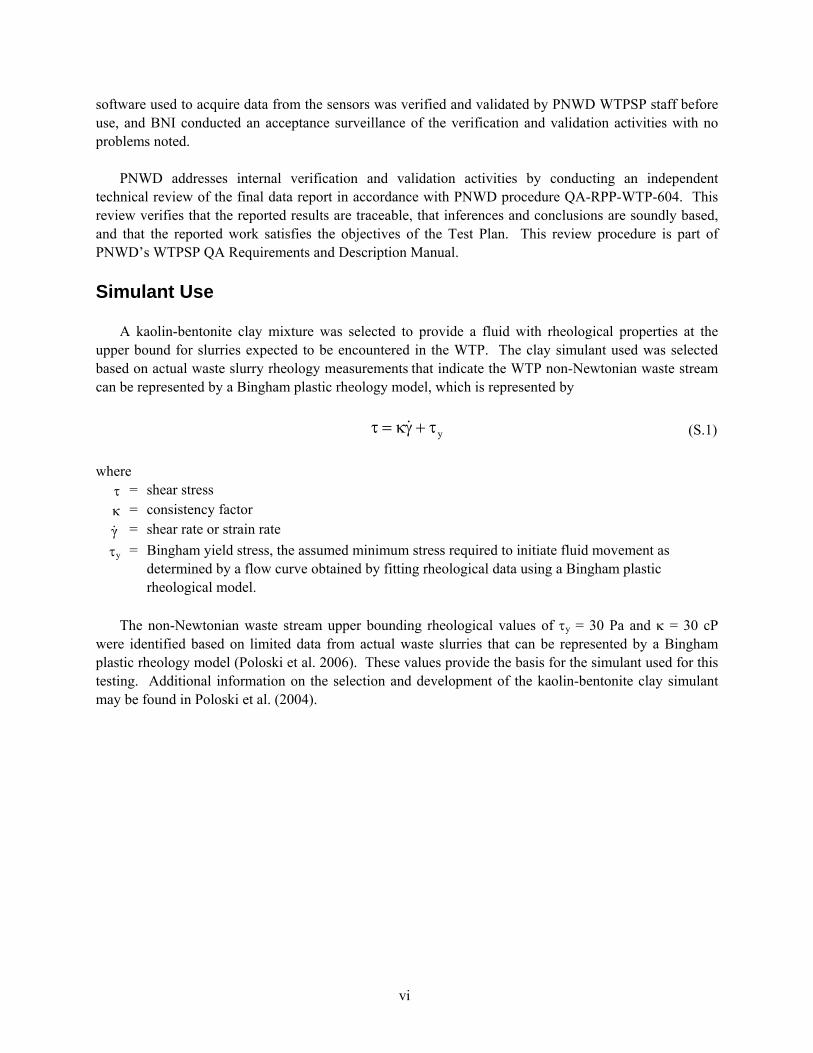
software used to acquire data from the sensors was verified and validated by PNWD WTPSP staff before use, and BNI conducted an acceptance surveillance of the verification and validation activities with no problems noted. PNWD addresses internal verification and validation activities by conducting an independent technical review of the final data report in accordance with PNWD procedure QA-RPP-WTP-604. This review verifies that the reported results are traceable, that inferences and conclusions are soundly based, and that the reported work satisfies the objectives of the Test Plan. This review procedure is part of PNWD’s WTPSP QA Requirements and Description Manual. Simulant Use A kaolin-bentonite clay mixture was selected to provide a fluid with rheological properties at the upper bound for slurries expected to be encountered in the WTP. The clay simulant used was selected based on actual waste slurry rheology measurements that indicate the WTP non-Newtonian waste stream can be represented by a Bingham plastic rheology model, which is represented by

yτ = κγ + τ& (S.1) where

τ = shear stress κ = consistency factor

γ& = shear rate or strain rate τy = Bingham yield stress, the assumed minimum stress required to initiate fluid movement as

determined by a flow curve obtained by fitting rheological data using a Bingham plastic rheological model.

The non-Newtonian waste stream upper bounding rheological values of τy = 30 Pa and κ = 30 cP were identified based on limited data from actual waste slurries that can be represented by a Bingham plastic rheology model (Poloski et al. 2006). These values provide the basis for the simulant used for this testing. Additional information on the selection and development of the kaolin-bentonite clay simulant may be found in Poloski et al. (2004).

vii

Discrepancies and Follow-on Tests To apply the test results in this report to an assessment of full-scale (i.e. plant-scale) mixing behavior in a pulse tube, additional information is needed, along with additional testing at different scales or analysis using an appropriate computational fluid dynamics (CFD) model. Full-scale refill functions will be needed to estimate the dimensionless refill velocity and acceleration. If the dimensionless acceleration and velocity at full scale are greater than or equal to values at half-scale, we expect the mixing results obtained at half-scale to be conservative since the jet Reynolds number will be larger at full-scale; mixing is expected to improve as the jet Reynolds number increases. However, if the dimensionless acceleration of the full-scale refill function is smaller than that at half scale, it is possible that the test results could be nonconservative. The location of the mixing line determined in the half-scale tests will also need to be estimated at full scale. This may be obtained by additional pulse tube mixing tests at different scales. Alternatively, it may be possible to estimate the location of the mixing line using an appropriate CFD model. Summary References Poloski AP, PA Meyer, LK Jagoda, and PR Hrma. 2004. Non-Newtonian Slurry Simulant Development and Selection for Pulsed Jet Mixer Testing. PNWD-3495 (WTP-RPT-111 Rev 0), Battelle – Pacific Northwest Division, Richland, Washington. Poloski AP, ST Arm, OP Bredt, TB Calloway, Y Onishi, RA Peterson, GL Smith, and HD Smith. 2006. Final Report: Technical Basis for HLW Vitrification Stream Physical and Rheological Property Bounding Conditions. PNWD-3675 (WTP-RPT-112 Rev 0), Battelle – Pacific Northwest Division, Richland, Washington.

ix

Contents

Testing Summary ......................................................................................................................................... iii

1.0 Introduction....................................................................................................................................... 1.1

2.0 Quality Requirements ....................................................................................................................... 2.1

3.0 Equipment Configuration ................................................................................................................. 3.1 3.1 HSLS Tank and Mixing System .............................................................................................. 3.1

3.1.1 PJM Assembly ............................................................................................................. 3.1 3.1.2 Sparger Assembly ........................................................................................................ 3.2

3.2 Instruments and Ancillary Systems ......................................................................................... 3.3 3.2.1 Analytical Instruments ................................................................................................. 3.3 3.2.2 Video Monitoring of Pulse Tube Mixing..................................................................... 3.3 3.2.3 Tracer Injection System ............................................................................................... 3.4 3.2.4 Core Sampling ............................................................................................................. 3.4

4.0 Pulse Tube Mixing Test Approach ................................................................................................... 4.1 4.1 Simulant................................................................................................................................... 4.1 4.2 Video Camera Monitoring of Pulse Tube Mixing ................................................................... 4.1 4.3 Pulse Tube Tracer Mixing Tests.............................................................................................. 4.2

4.3.1 Pulse Tube Tracer Mixing Test Approach................................................................... 4.2 4.3.2 Tracer Addition Approach ........................................................................................... 4.5 4.3.3 Grab Sampling ............................................................................................................. 4.6 4.3.4 Core Sampling ............................................................................................................. 4.6

5.0 Mixing Test Results .......................................................................................................................... 5.1 5.1 Video Observations of Surface Mixing ................................................................................... 5.1

5.1.1 Observations of Surface Disturbances ......................................................................... 5.3 5.1.2 Analysis of Surface Disturbance Observations............................................................ 5.4

5.2 Pulse Tube Tracer Mixing Test: Half-Stroke ........................................................................ 5.10 5.2.1 Mixing Test Approach: Half-Stroke .......................................................................... 5.10

5.3 Comparison of Video Camera Results and Tracer Results.................................................... 5.20 5.4 Interpretation and Application of Results.............................................................................. 5.23

6.0 Pulse Tube Tracer Mixing Test: Full Stroke..................................................................................... 6.1

7.0 Conclusions and Recommendations ................................................................................................. 7.1

8.0 References......................................................................................................................................... 8.1

Appendix – Comparison of Experimental Half and Full Strokes with Ideal Half and Full Strokes and Definition of Full-Stroke Equivalent .................................................................... A.1

x

Figures

3.1 Plan View of the Half-Scale Lag Storage Tank............................................................................... 3.2 3.2 Video Assembly Installed in Pulse Tube #7.................................................................................... 3.4 3.3 Top View of Core Sampling Ports in Relation to Refill Jet Upwell................................................ 3.5 4.1 Characterization of Core Shortening ............................................................................................... 4.7 5.1 Illustration of the Progression of a Typical Video Observation Surface Mixing Test .................... 5.1 5.2 Illustration of Threshold Mixing Cases ........................................................................................... 5.2 5.3 Examples of Gravity-Driven PJM Refill Behavior ......................................................................... 5.5 5.4 Examples of Vacuum-Driven PJM Refill Behavior ........................................................................ 5.6 5.5 Surface Disturbance Observations Correlated with Instantaneous Nozzle Velocity....................... 5.7 5.6 Comparing End of Surface Motion Data with Nonlinear Model .................................................... 5.9

5.7 Surface Disturbance Observations Correlated with the Parameter u0d0t .................................. 5.10 5.8 PJM Drive Functions Used for the Mixing Tests .......................................................................... 5.14 5.9 Relationship Between Initial PJM Refill Level and Stroke Percentage in HSLS ......................... 5.14 5.10 Yield Stress of Simulant During the Tracer Test........................................................................... 5.15 5.11 Core Sample Results for Run 2 ..................................................................................................... 5.16 5.12 Core Sample Results for Run 3 ..................................................................................................... 5.17 5.13 Core Sample Results for Run 4 ..................................................................................................... 5.18 5.14 Core Sample Results for Run 5 ..................................................................................................... 5.18 5.15 Core Sample Results for Run 6 ..................................................................................................... 5.19 5.16 Core Sample Results for Run 7 ..................................................................................................... 5.19 5.17 Core Sample Results for Run 8 ..................................................................................................... 5.20 5.18 Refill Velocity and Level Used in the Mixing Tracer Tests.......................................................... 5.21 5.19 Mixing Test Refill Curves Compared with Video Surface Disturbance Data:

Instantaneous Nozzle Velocity Correlation ................................................................................... 5.22 5.20 Mixing Test Refill Curves Compared with Video Surface Disturbance Data:

Time Parameter Correlation .......................................................................................................... 5.23 5.21 Fitting the Video Data Results to the Tracer Test Mixing Interface ............................................. 5.24 5.22 Pulse Tube Refill Mixing Behavior at Half Scale ......................................................................... 5.24 5.23 Effect of Stroke Length on Pulse Tube Mixing at Half Scale ....................................................... 5.25 6.1 Approximate PJM Refill Velocity Profile for Full-Stroke Equivalent Test .................................... 6.4 6.2 Core Sample Results for Run 2 ....................................................................................................... 6.6 6.3 Core Sample Results for Run 3 ....................................................................................................... 6.7 6.4 Core Sample Results for Run 4 ...................................................................................................... 6.7 6.5 Core Sample Results for Run 5 ....................................................................................................... 6.8 6.6 Core Sample Results for Run 6 ...................................................................................................... 6.8 6.7 Core Sample Results for Run 7 ...................................................................................................... 6.9

xi

6.8 Core Sample Results for Run 8 ...................................................................................................... 6.9

6.9 Interpolated Cl- Concentrations at Depths of 6 and 30 inches as a Function of Full-Stroke Equivalent PJM Cycles .............................................................................................. 6.10

Tables

S.1 Summary of Test Objectives and Results.......................................................................................... iv S.2 Test Exceptions ................................................................................................................................. iv S.3 Success Criteria .................................................................................................................................. v 3.1 PNWD Analytical Instruments Used in the Mixing/Controller Testing.......................................... 3.3 4.1 Test Conditions for Video Monitoring of Pulse Tube Mixing ........................................................ 4.2 4.2 Half-Stroke Pulse Tube Tracer Mixing Test Run Sequence ........................................................... 4.3 4.3 Half-Stroke Mixing Conditions ....................................................................................................... 4.3 4.4 Full-Stroke Pulse Tube Tracer Mixing Test Run Sequence ............................................................ 4.4 4.5 Full-Stroke Mixing Conditions........................................................................................................ 4.5 5.1 Surface Disturbance Results from Video Monitoring of Pulse Tube Mixing ................................. 5.3 5.2 Conditions for Threshold Surface Disturbances.............................................................................. 5.4 5.3 Pulse Tube Mixing Tracer Test Conditions................................................................................... 5.11 5.4 PJM Stroke Characteristics Achieved in the Tracer Mixing Test ................................................. 5.15 5.5 Percent Mixed Values for Operation at Half Stroke...................................................................... 5.20 6.1 Pulse Tube Mixing Tracer Test Conditions..................................................................................... 6.2 6.2 Yield Stress of Simulant During the Full-Stroke Equivalent Tracer Test ....................................... 6.4 6.3 Percent Mixed Values for Operation at Full-Stroke Equivalent.................................................... 6.10

1.1

1.0 Introduction The U.S. Department of Energy (DOE) Office of River Protection’s Waste Treatment Plant (WTP) is being designed and built to pretreat and then vitrify a large portion of the wastes in Hanford’s 177 underground waste storage tanks. The WTP consists of three primary facilities: pretreatment, low-activity waste (LAW) vitrification, and high-level waste (HLW) vitrification. The pretreatment facility receives waste feed from the Hanford tank farms and separates it into 1) a high-volume, low-activity liquid stream stripped of most solids and radionuclides and 2) a much smaller-volume HLW slurry containing most of the solids and most of the radioactivity. Many of the vessels in the pretreatment facility will contain pulse jet mixers (PJMs) that will provide some or all of the mixing in the vessels. This technology was selected for use in so-called “black cell” regions of the WTP where maintenance capability will not be available for the operating life of the WTP. PJM technology was selected for use in these regions because it has no moving mechanical parts that require maintenance. The vessels with the most concentrated slurries will also be mixed with air spargers and/or steady jets in addition to the mixing provided by the PJMs. A large amount of testing and development work directed at the mixing systems in vessels expected to contain the concentrated slurries has been completed and is summarized in Meyer et al. (2005). This work was directed at mixing and retention/release of potentially flammable gases from the contents of these vessels. Most of this work was conducted with the PJMs operating in a full-stroke mode. For quantitative purposes in this report, we define a full stroke as a stroke length sufficient to expel 85% of the volume of the pulse tube. As part of an effort to prevent potentially damaging overblows of the pulse tubes, an option to operate at half-stroke was considered. A half stroke is defined as one half of a full stroke or a stroke length sufficient to expel 42.5% of the pulse tube volume. It became necessary to investigate the degree of mixing in the pulse tubes operated in this manner because the half-stroke mode of operation expels only a fraction of the pulse tube contents. The tests described in this report were directed at evaluating the extent of mixing of the pulse tube contents with stroke lengths ranging from half to full stroke using the following techniques:

A video camera inserted into the top of one of the pulse tubes was used to observe the behavior of the slurry remaining in the PJM following the drive phase and to determine the height of slurry jet penetration during PJM refill as affected by PJM nozzle refill velocity.

A sodium chloride tracer was used to assess the extent of mixing in the pulse tube operated at half- and full stroke as a function of the number of pulses. The tracer was also used to determine the mixing cavern size as a percentage of the slurry volume.

2.1

2.0 Quality Requirements Battelle – Pacific Northwest Division’s (PNWD) Quality Assurance Program is based on the require-ments defined in the U.S. Department of Energy (DOE) Order 414.1A, Quality Assurance, and 10 CFR 830, Energy/Nuclear Safety Management, Subpart A–Quality Assurance Requirements (a.k.a. the Quality Rule). PNWD has chosen to implement the requirements of DOE Order 414.1A and 10 CFR 830, Subpart A by integrating them into the Laboratory's management systems and daily operating processes. The procedures needed to implement the requirements are documented through PNWD's Standards-Based Management System. PNWD implements the WTP quality requirements by performing work in accordance with the PNWD WTP Support Project quality assurance project plan (QAPjP) approved by the WTP Quality Assurance (QA) organization. This work was performed to the quality requirements of NQA-1-1989 Part I, Basic and Supplementary Requirements, NQA-2a-1990 Part 2.7, and DOE/RW-0333P Rev. 13, Quality Assurance Requirements and Description. These quality requirements are implemented through PNWD's WTP Support Project (WTPSP) Quality Assurance Requirements and Description Manual. The analytical requirements are implemented through WTPSP’s Statement of Work (WTPSP-SOW-005) with the Radiochemical Processing Laboratory Analytical Services Operations. Experiments that were not method-specific were performed in accordance with PNWD procedures QA-RPP-WTP-1101, “Scientific Investigations,” and QA-RPP-WTP-1201, “Calibration Control System,” ensuring that sufficient data were taken with properly calibrated measurement and test equipment to obtain quality results. Reportable measurements of distance were made using standard commercially available equipment (e.g., tape measure, scale) and needed no traceable calibration requirements. All other test equipment generating reportable data were calibrated according to the PNWD’s WTPSP Quality Assurance program. The DASYLab software used to acquire data from the sensors was verified and validated by PNWD WTPSP staff prior to use, and BNI conducted an acceptance surveillance of the verification and validation activities with no problems noted. PNWD addressed internal verification and validation activities by conducting an independent technical review of the final data and this report in accordance with PNWD procedure QA-RPP-WTP-604. This review verified that the reported results are traceable, that inferences and conclusions are soundly based, and that the reported work satisfies the Test Plan objectives. This review procedure is part of PNWD's WTPSP Quality Assurance Requirements and Description Manual.

3.1

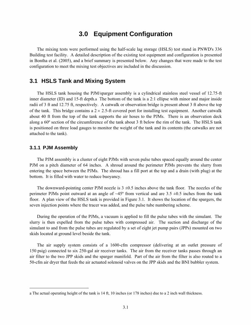
3.0 Equipment Configuration The mixing tests were performed using the half-scale lag storage (HSLS) test stand in PNWD's 336 Building test facility. A detailed description of the existing test equipment and configuration is presented in Bontha et al. (2005), and a brief summary is presented below. Any changes that were made to the test configuration to meet the mixing test objectives are included in the discussion.

3.1 HSLS Tank and Mixing System The HSLS tank housing the PJM/sparger assembly is a cylindrical stainless steel vessel of 12.75-ft inner diameter (ID) and 15-ft depth.a The bottom of the tank is a 2:1 ellipse with minor and major inside radii of 3 ft and 12.75 ft, respectively. A catwalk or observation bridge is present about 3 ft above the top of the tank. This bridge contains a 2 × 2.5-ft covered port for installing test equipment. Another catwalk about 40 ft from the top of the tank supports the air hoses to the PJMs. There is an observation deck along a 60º section of the circumference of the tank about 3 ft below the rim of the tank. The HSLS tank is positioned on three load gauges to monitor the weight of the tank and its contents (the catwalks are not attached to the tank).

3.1.1 PJM Assembly The PJM assembly is a cluster of eight PJMs with seven pulse tubes spaced equally around the center PJM on a pitch diameter of 64 inches. A shroud around the perimeter PJMs prevents the slurry from entering the space between the PJMs. The shroud has a fill port at the top and a drain (with plug) at the bottom. It is filled with water to reduce buoyancy. The downward-pointing center PJM nozzle is 3 ±0.5 inches above the tank floor. The nozzles of the perimeter PJMs point outward at an angle of ~45º from vertical and are 3.5 ±0.5 inches from the tank floor. A plan view of the HSLS tank is provided in Figure 3.1. It shows the location of the spargers, the seven injection points where the tracer was added, and the pulse tube numbering scheme. During the operation of the PJMs, a vacuum is applied to fill the pulse tubes with the simulant. The slurry is then expelled from the pulse tubes with compressed air. The suction and discharge of the simulant to and from the pulse tubes are regulated by a set of eight jet pump pairs (JPPs) mounted on two skids located at ground level beside the tank. The air supply system consists of a 1600-cfm compressor (delivering at an outlet pressure of 150 psig) connected to six 250-gal air receiver tanks. The air from the receiver tanks passes through an air filter to the two JPP skids and the sparger manifold. Part of the air from the filter is also routed to a 50-cfm air dryer that feeds the air actuated solenoid valves on the JPP skids and the BNI bubbler system.

a The actual operating height of the tank is 14 ft, 10 inches (or 178 inches) due to a 2 inch wall thickness.

3.2

Sparger (7)

Peroxide Injection Point (7)

1 2

3

4 5

6

7

8

Bridge above tank: Position is approximate

Grab Sample location (low and high position)

Grab Sample location (low position)

Tracer Injection (7)

Figure 3.1. Plan View of the Half-Scale Lag Storage Tank

3.1.2 Sparger Assembly In addition to the PJMs, the HSLS tank is equipped with a set of seven spargers spaced equally around the perimeter at a pitch diameter of 110 inches and positioned at an elevation ~6 inches from the tank floor. The sparger tubes are made from a 1.5-inch schedule 10 stainless steel (SS) pipe (1.682-inch ID) with four 45º triangular cutouts at the discharge end (Bontha et al. 2005). The air flow to the spargers is regulated through a manifold on the mezzanine adjacent to the HSLS tank. The manifold consists of two lines for regulating the air flow under normal (main) operation and idle operation. Sparger air flow is switched from the main flow to the idle flow loop manually using ball valves installed in the headers of the two flow loops. Flow meters on the primary and idle flow lines for each of the spargers, along with pressure gauges and temperature sensors at the inlet and outlet of the

3.3

flow meters, enable the conversion of the air flow rates from standard cubic feet per minute (scfm) to actual cubic feet per minute (acfm) at the sparger nozzle. During the mixing test, the spargers were used only to homogenize the tank contents before and after the tracer testing.

3.2 Instruments and Ancillary Systems

3.2.1 Analytical Instruments The analytical instruments listed in Table 3.1 were used to collect and record data during the testing.

Table 3.1. PNWD Analytical Instruments Used in the Mixing/Controller Testing

Parameter Sensor Type Manufacturer Model Qty Range Unit AccuracyPJM Pressure Pressure transmitter E+H PMP 135-A4G01R4R 8 0 to 150 psia ± 0.75 psia

Tank Surface Level Laser level transmitter Optech Sentinel 3100 4 0.2 to 150 M ± 5 mm

Tank Temperature Type J thermocouple

Superior Sensors SA2-J412-1U-168 2 -100 to 300 °C ± 2 °C

Tank Weight Load cells BLH Z-Blok, 100K lb 3 0 to 300k lb ± 100 lb Sparger Inlet Air Pressure Pressure transmitter Cecomp F4L100PSIA 7 0 to 100 psia ±0.25 psia

Sparger Outlet Air Pressure Pressure transmitter Cecomp F4L30PSIA 7 0 to 30 psia ±0.075 psia

Sparger Air Inlet Temperature

Type T thermocouple Eustis MCT41U6-

0000M0 3 0 to 200 °C ± 1°C

Sparger Air Outlet Temperature

Type T thermocouple Eustis MCT41U6-

0000M0 3 0 to 200 °C ± 1°C

Main Sparge Air Flow Rate Flow meter Hedland H791B-100-EL 7 10 to 100 scfm ± 2 scfm

Weight Weighing balance Mettler-Toledo AE200 1 0 to 200 g ±0.0001 gWeight Weighing balance Sartorius BP3100S 1 0 to 3000 g ± 0.01 g Weight Weighing balance Sartorius E12000S 1 0 to 10000 g ± 0.1 g

3.2.2 Video Monitoring of Pulse Tube Mixing Mixing in the pulse tube was observed using a miniature video camera mounted in the top of pulse tube #7 (Figure 3.2). Mixing was observed as a visual surface agitation of the simulant induced by the incoming jet from the nozzle during pulse tube refill. The camera was mounted on a ¾-inch SS pipe inserted through the 2-inch-ID SS cross on top of the pulse tube after removal of the level probe. The area in front of the camera was illuminated by an array of light emitting diodes (LEDs) placed around the camera lens. The camera was a few inches below the top of the PJM dish-head. To prevent the video camera from submersion in simulant, the simulant level was lowered and maintained a few inches below the camera. In addition, the pulse tube refill cycle was adjusted to prevent the simulant from rising past the camera into the air supply line above the pulse tube.

3.4

Simulant Level in Tank ~10-in

~4-ft long Spool Piece

2-in Cross

0.75-in Support Pipe

Video Camera

Figure 3.2. Video Assembly Installed in Pulse Tube #7

3.2.3 Tracer Injection System The tracer injection system injects NaCl tracer at seven separate locations within the highly mixed region of the tank above the spargers and the PJM nozzles. The tracer injection lines are located between two adjacent sparger tubes and routed along the wall of the tank up to an elevation of ~6 inches above the bottom of the sparger tube. The injection lines then extend radially inward to a radius of 55 inches. During the tracer injection, a combination of seven flow controllers and a small pump enable metering equal tracer flow rates at the seven injection points.

3.2.4 Core Sampling Core samples were collected during the tracer mixing tests by accessing the test pulse tube from the top. A number of samples were collected from the center of the pulse tube by inserting the core sampler into the same port used for the video camera (see Figure 3.2). During the full-stroke mixing test, an additional sample port was installed in the top of the test pulse tube (PJM #6 in the full-stroke test). This port was located radially outward from the center of the tank approximately 6.5 inches from the center of the pulse tube. This location was chosen based on video camera observations which indicated that this was the most likely location for unmixed simulant due to the location of the refill jet upwell (Figure 3.3).

3.5

PJM nozzle

Center core sample port

Edge core sample port

General area of refill jet upwell

Pulse tube

Figure 3.3. Top View of Core Sampling Ports in Relation to Refill Jet Upwell (not to scale)

4.1

4.0 Pulse Tube Mixing Test Approach This section describes the test conditions for video camera monitoring and sodium chloride tracer mixing measurements. The simulant used for all of the testing is also described.

4.1 Simulant The simulant used in the video camera and chloride tracer mixing tests was a mixture of kaolin and bentonite clay in water. This simulant has been used successfully in previous PJM/sparger testing in the Applied Process Engineering Laboratory (APEL) and 336 Building test stands (Poloski et al. 2004a, Bontha et al. 2005). Multiple rheological samples of the simulant were taken during the tests to ensure that its yield stress was 30 ±5 Pa, as specified in the test plan. Actual values are reported with the results in Sections 5 and 6. Simulant rheology was measured using a TA Instruments AR 2000 rheometer with a concentric cylinder sensor. This model is a controlled stress rheometer equipped with an air bearing and a Peltier plate for temperature control. The instrument performance was checked before the testing started and then periodically throughout the testing using calibrated standard oils.

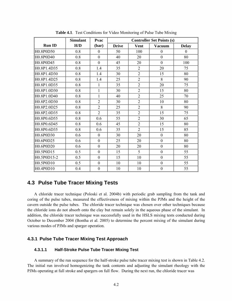
4.2 Video Camera Monitoring of Pulse Tube Mixing The PJM operating conditions for the video monitoring of mixing in the pulse tube are shown in Table 4.1. The first column is the run identifier, the second column is the simulant height (H) to tank diameter (D) ratio, and the third column (Pvac) indicates the pressure setting of the regulator on the vacuum (suction) leg of the JPP. When Pvac is zero, refill of the pulse tube was due solely to the difference in simulant level outside the pulse tube relative to the level inside of the pulse tube. As Pvac is increased, the vacuum applied to the pulse tube increases and results in an increase in the nozzle refill velocity. The last four columns represent the PJM controller set point times for the drive, vent, vacuum, and delay phases of the cycle. The set of test conditions defined in Table 4.1 provides a range of simulant levels and nozzle refill velocities. The level in the pulse tube at the start of a refill was controlled by a combination of the starting simulant level and the drive pressure/time. At a given simulant level, an increase in the drive time reduced the simulant level in the pulse tube at the start of refill. A range of drive times was assessed for each set of simulant and refill conditions in an attempt to find the level at which the start and end of mixing converged to approximately the same time. Various nozzle refill velocities were obtained by varying the difference in simulant level inside the pulse tube relative to the level in the tank and by varying the vacuum in the pulse tube during refill. Observations of at least three cycles were obtained at each set of conditions in Table 4.1.

4.2

Table 4.1. Test Conditions for Video Monitoring of Pulse Tube Mixing

Controller Set Points (s) Run ID

Simulant H/D

Pvac (bar) Drive Vent Vacuum Delay

H0.8P0D50 0.8 0 50 100 0 0 H0.8P0D40 0.8 0 40 20 0 80 H0.8P0D45 0.8 0 45 20 0 100 H0.8P1.4D35 0.8 1.4 35 2 20 75 H0.8P1.4D30 0.8 1.4 30 2 15 80 H0.8P1.4D25 0.8 1.4 25 2 8 90 H0.8P1.0D35 0.8 1 35 2 20 75 H0.8P1.0D30 0.8 1 30 2 15 80 H0.8P1.0D40 0.8 1 40 2 25 70 H0.8P2.0D30 0.8 2 30 2 10 80 H0.8P2.0D25 0.8 2 25 2 8 90 H0.8P2.0D35 0.8 2 35 2 15 75 H0.8P0.6D55 0.8 0.6 55 2 30 65 H0.8P0.6D45 0.8 0.6 45 2 15 80 H0.8P0.6D35 0.8 0.6 35 2 15 85 H0.6P0D30 0.6 0 30 20 0 80 H0.6P0D25 0.6 0 25 20 0 80 H0.6P0D20 0.6 0 20 20 0 80 H0.5P0D15 0.5 0 15 5 0 55 H0.5P0D15-2 0.5 0 15 10 0 55 H0.5P0D10 0.5 0 10 10 0 55 H0.4P0D10 0.4 0 10 10 0 55

4.3 Pulse Tube Tracer Mixing Tests A chloride tracer technique (Poloski et al. 2004b) with periodic grab sampling from the tank and coring of the pulse tubes, measured the effectiveness of mixing within the PJMs and the height of the cavern outside the pulse tubes. The chloride tracer technique was chosen over other techniques because the chloride ions do not absorb onto the clay but remain solely in the aqueous phase of the simulant. In addition, the chloride tracer technique was successfully used in the HSLS mixing tests conducted during October to December 2004 (Bontha et al. 2005) to determine the percent mixing of the simulant during various modes of PJMs and sparger operation.

4.3.1 Pulse Tube Tracer Mixing Test Approach

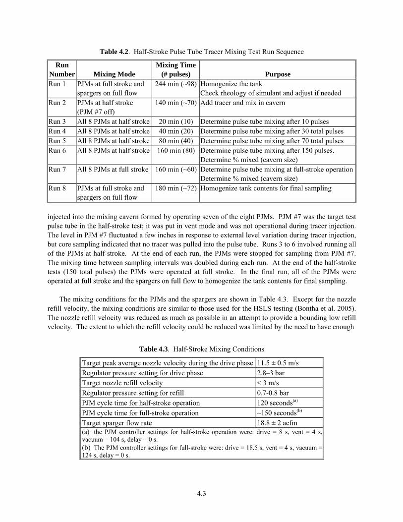
4.3.1.1 Half-Stroke Pulse Tube Tracer Mixing Test A summary of the run sequence for the half-stroke pulse tube tracer mixing test is shown in Table 4.2. The initial run involved homogenizing the tank contents and adjusting the simulant rheology with the PJMs operating at full stroke and spargers on full flow. During the next run, the chloride tracer was

4.3

Table 4.2. Half-Stroke Pulse Tube Tracer Mixing Test Run Sequence

Run Number Mixing Mode

Mixing Time(# pulses) Purpose

Run 1 PJMs at full stroke and spargers on full flow

244 min (~98) Homogenize the tank Check rheology of simulant and adjust if needed

Run 2 PJMs at half stroke (PJM #7 off)

140 min (~70) Add tracer and mix in cavern

Run 3 All 8 PJMs at half stroke 20 min (10) Determine pulse tube mixing after 10 pulses Run 4 All 8 PJMs at half stroke 40 min (20) Determine pulse tube mixing after 30 total pulses Run 5 All 8 PJMs at half stroke 80 min (40) Determine pulse tube mixing after 70 total pulses Run 6 All 8 PJMs at half stroke 160 min (80) Determine pulse tube mixing after 150 pulses.

Determine % mixed (cavern size) Run 7 All 8 PJMs at full stroke 160 min (~60) Determine pulse tube mixing at full-stroke operation

Determine % mixed (cavern size) Run 8 PJMs at full stroke and

spargers on full flow 180 min (~72) Homogenize tank contents for final sampling

injected into the mixing cavern formed by operating seven of the eight PJMs. PJM #7 was the target test pulse tube in the half-stroke test; it was put in vent mode and was not operational during tracer injection. The level in PJM #7 fluctuated a few inches in response to external level variation during tracer injection, but core sampling indicated that no tracer was pulled into the pulse tube. Runs 3 to 6 involved running all of the PJMs at half-stroke. At the end of each run, the PJMs were stopped for sampling from PJM #7. The mixing time between sampling intervals was doubled during each run. At the end of the half-stroke tests (150 total pulses) the PJMs were operated at full stroke. In the final run, all of the PJMs were operated at full stroke and the spargers on full flow to homogenize the tank contents for final sampling. The mixing conditions for the PJMs and the spargers are shown in Table 4.3. Except for the nozzle refill velocity, the mixing conditions are similar to those used for the HSLS testing (Bontha et al. 2005). The nozzle refill velocity was reduced as much as possible in an attempt to provide a bounding low refill velocity. The extent to which the refill velocity could be reduced was limited by the need to have enough

Table 4.3. Half-Stroke Mixing Conditions

Target peak average nozzle velocity during the drive phase 11.5 ± 0.5 m/s Regulator pressure setting for drive phase 2.8–3 bar Target nozzle refill velocity < 3 m/s Regulator pressure setting for refill 0.7-0.8 bar PJM cycle time for half-stroke operation 120 seconds(a) PJM cycle time for full-stroke operation ~150 seconds(b) Target sparger flow rate 18.8 ± 2 acfm (a) the PJM controller settings for half-stroke operation were: drive = 8 s, vent = 4 s, vacuum = 104 s, delay = 0 s. (b) The PJM controller settings for full-stroke were: drive = 18.5 s, vent = 4 s, vacuum = 124 s, delay = 0 s.

4.4

vacuum to draw the simulant to an elevation near the top of the pulse tube. With the simulant level at an H/D of 0.58, the vacuum had to pull the simulant in the pulse tube several feet above the level in the tank. For full-stroke operation, the slow refill increased the total cycle time from 120 seconds to ~150 seconds.

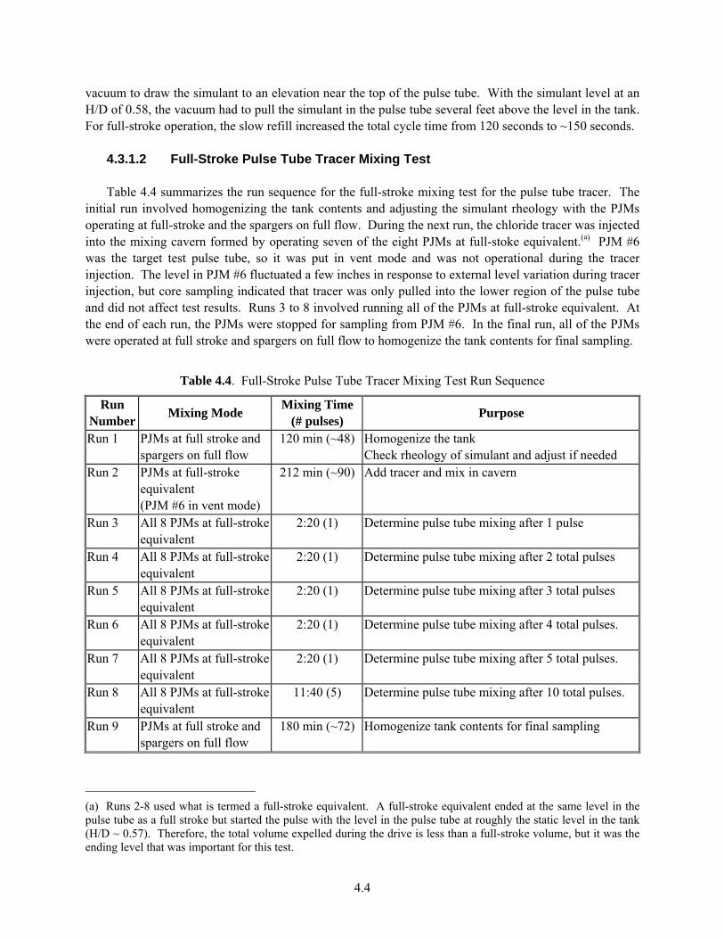
4.3.1.2 Full-Stroke Pulse Tube Tracer Mixing Test Table 4.4 summarizes the run sequence for the full-stroke mixing test for the pulse tube tracer. The initial run involved homogenizing the tank contents and adjusting the simulant rheology with the PJMs operating at full-stroke and the spargers on full flow. During the next run, the chloride tracer was injected into the mixing cavern formed by operating seven of the eight PJMs at full-stoke equivalent.(a) PJM #6 was the target test pulse tube, so it was put in vent mode and was not operational during the tracer injection. The level in PJM #6 fluctuated a few inches in response to external level variation during tracer injection, but core sampling indicated that tracer was only pulled into the lower region of the pulse tube and did not affect test results. Runs 3 to 8 involved running all of the PJMs at full-stroke equivalent. At the end of each run, the PJMs were stopped for sampling from PJM #6. In the final run, all of the PJMs were operated at full stroke and spargers on full flow to homogenize the tank contents for final sampling.

Table 4.4. Full-Stroke Pulse Tube Tracer Mixing Test Run Sequence

Run Number Mixing Mode Mixing Time

(# pulses) Purpose


120 min (~48) Homogenize the tank Check rheology of simulant and adjust if needed

Run 2 PJMs at full-stroke equivalent (PJM #6 in vent mode)

212 min (~90) Add tracer and mix in cavern

Run 3 All 8 PJMs at full-stroke equivalent

2:20 (1) Determine pulse tube mixing after 1 pulse


2:20 (1) Determine pulse tube mixing after 2 total pulses


2:20 (1) Determine pulse tube mixing after 3 total pulses


2:20 (1) Determine pulse tube mixing after 4 total pulses.






180 min (~72) Homogenize tank contents for final sampling

(a) Runs 2-8 used what is termed a full-stroke equivalent. A full-stroke equivalent ended at the same level in the pulse tube as a full stroke but started the pulse with the level in the pulse tube at roughly the static level in the tank (H/D ~ 0.57). Therefore, the total volume expelled during the drive is less than a full-stroke volume, but it was the ending level that was important for this test.

4.5

Table 4.5 shows the mixing conditions for the PJMs and the spargers. Except for the nozzle refill velocity, the mixing conditions are similar to those for the half-stroke mixing test. The nozzle refill velocity was reduced as much as possible in an attempt to provide a bounding low refill velocity. This was accomplished by allowing the refill to occur with the PJMs in the vent mode (i.e., no vacuum). The refill of the pulse tube was induced by the static height difference between simulant level inside and outside of the pulse tube. A short period of vacuum was applied to ensure that the simulant level in the pulse tube reached the level of the simulant in the tank.

Table 4.5. Full-Stroke Mixing Conditions

Target peak average nozzle velocity during the drive phase 11.5 ± 0.5 m/s Regulator pressure setting for drive phase 2.8–3.2 bar Target nozzle refill velocity < 3.5 m/s Regulator pressure setting for refill 0.8-0.9 bar PJM cycle time for full-stroke equivalent operation ~140 seconds(a) PJM cycle time for full-stroke operation ~150 seconds(b) Target sparger flow rate 18.8 ± 2 acfm (a) The PJM controller settings for full-stroke equivalent were as follows: drive = 8.4 s, vent = 90 s, vacuum = 6 s, delay = 30 s. (b) The PJM controller settings for full-stroke were as follows: drive = 18.5 s, vent = 4 s, vacuum = 124 s, delay = 0 s.

4.3.2 Tracer Addition Approach The tracer injection system is described in Section 3.2.3. The following sections present the details of the approach used to add the tracer.

4.3.2.1 Tracer Addition; Half-Stroke Prior to the start of the half-stroke mixing test, the tracer was injected as a concentrated salt solution of ~20 to 25 wt% NaCl dissolved in water. Because the time to mix was not critical to the testing, the tracer was injected into the simulant over a 20-minute time span (included 4 minutes of water flush) during which seven of the eight PJMs(a) operated continuously. The relatively slow injection along with the PJM operation minimized the possibility that the tracer would be trapped in unmixed bubbles. Operation of the seven PJMs continued for another 120 minutes to provide a reasonably good tracer distribution in the mixed region.

4.3.2.2 Tracer Addition, Full-Stroke Before starting the full-stroke mixing test, the tracer was injected as a concentrated salt solution of ~20 to 25 wt% NaCl dissolved in water. The tracer was injected into the simulant over a 39-minute time

(a) One of the radial PJMs (PJM #7) was not operated during the tracer injection to enable coring of the PJM for determining the time-dependent chloride ion concentration inside of the pulse tube.

4.6

span followed by 22 minutes of water flush, during which seven of the eight PJMs(a) operated continuously. The relatively slow injection along with the PJM operation minimized the possibility that the tracer would be trapped in unmixed bubbles. Operation of the seven PJMs continued for another 151 minutes to provide a reasonably good tracer distribution in the mixed region.

4.3.3 Grab Sampling Grab samples were collected periodically from two locations in the tank to determine the baseline salt and cavern concentrations. One grab sample was taken from the southeast quadrant of the tank near PJM #5 (see Figure 3.1) at ~3 ft above the centerline elevation of the tank bottom. A second sample was collected near the surface (sampling depth <1 ft) of the simulant at the same location. A third grab sample was collected from the northwest quadrant of the tank near PJM #1, ~3 ft above the centerline elevation of the tank bottom. The grab samples were collected using a 100-mL syringe mounted at one end of a long pipe. The sampler configuration was such that the plunger on the syringe could be operated by a person standing on the bridge above the tank. Because of the long lengths of the sampler pipe (~20 ft), 2-inch-outer diameter (OD) PVC tubes mounted along the railing of the bridge were used to guide the sampler to the appropriate position. The uncertainty in sample elevation using this method was estimated to be ±3 inches. While the PJMs were operating, the syringe with the plunger pushed all the way down was lowered to the sampling position and left there by clamping the other end to the railing of the bridge. At the appropriate sampling time, the mixing was turned off and the plunger slowly pulled out to fill the syringe with the clay slurry. Then the syringe was carefully pulled up out of the tank and emptied into a sample bottle. The syringe was rinsed with deionized water and returned to its sampling position with the plunger all the way down.

4.3.4 Core Sampling Core sampling from the pulse tubes was performed to determine the tracer concentration profile in the pulse tube. The core sampling method involved vibrating a 1-inch-ID PVC pipe into the simulant all the way to the bottom of the pulse tube. Loss of sample during removal of the core was minimized by inflating a balloon installed near the bottom of the PVC sampling pipe. After removal from the tank, the cores were frozen and cut into 3-inch-long pieces. For the half-stroke mixing test, every fourth piece was homogenized and analyzed by ion chromatography to determine the chloride ion concentration. Based on the initial results, additional samples were selected and analyzed to better define the mixing interface in the pulse tube. For the full-stroke mixing test, core segments were selected for analysis from various locations in the cores. Core samples were shortened slightly by several different processes. This caused compaction of the sample in the core tube or a loss of sample at or near the bottom of the core tube. Core shortening in the

(a) One of the radial PJMs (PJM #6) was not operated during the tracer injection to enable coring of the PJM for determining the time-dependent chloride ion concentration inside of the pulse tube.

4.7

current application probably occurred due to the increased friction as the coring tube was filled, excluding some of the sample in the lower portion of the pulse tube (Morton and White 1997, Blomqvist 1991). To reduce core shortening, the inside of the core tube was washed with water prior to insertion, and insertion was performed at a slow, controlled rate. To characterize the core shortening, a series of tests was conducted in which the coring tube was inserted to various depths and the simulant level inside and outside the coring tube noted. The sample level inside the coring tube was detected by shining a flashlight through the tube and noting the location of the shadow caused by the clay. The amount of shortening as a function of insertion depth is shown in Figure 4.1. No significant shortening was observed for insertion depths less than about 32 inches. These results were used to correct the chloride tracer core sample results to a true depth in the pulse tubes.

02468

1012141618

96 84 72 60 48 36 24 12

Insertion Depth (inches)

Am

ount

of S

horte

ning

(in

ches

)

Figure 4.1. Characterization of Core Shortening

5.1

5.0 Mixing Test Results

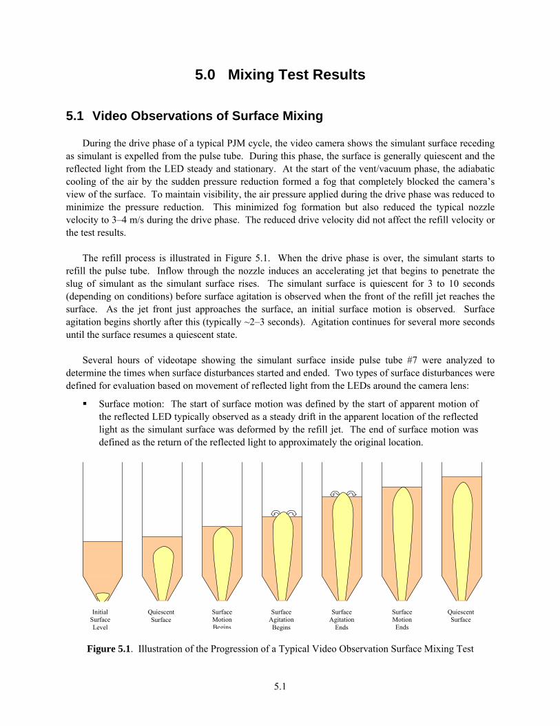
5.1 Video Observations of Surface Mixing During the drive phase of a typical PJM cycle, the video camera shows the simulant surface receding as simulant is expelled from the pulse tube. During this phase, the surface is generally quiescent and the reflected light from the LED steady and stationary. At the start of the vent/vacuum phase, the adiabatic cooling of the air by the sudden pressure reduction formed a fog that completely blocked the camera’s view of the surface. To maintain visibility, the air pressure applied during the drive phase was reduced to minimize the pressure reduction. This minimized fog formation but also reduced the typical nozzle velocity to 3–4 m/s during the drive phase. The reduced drive velocity did not affect the refill velocity or the test results. The refill process is illustrated in Figure 5.1. When the drive phase is over, the simulant starts to refill the pulse tube. Inflow through the nozzle induces an accelerating jet that begins to penetrate the slug of simulant as the simulant surface rises. The simulant surface is quiescent for 3 to 10 seconds (depending on conditions) before surface agitation is observed when the front of the refill jet reaches the surface. As the jet front just approaches the surface, an initial surface motion is observed. Surface agitation begins shortly after this (typically ~2–3 seconds). Agitation continues for several more seconds until the surface resumes a quiescent state. Several hours of videotape showing the simulant surface inside pulse tube #7 were analyzed to determine the times when surface disturbances started and ended. Two types of surface disturbances were defined for evaluation based on movement of reflected light from the LEDs around the camera lens:

Surface motion: The start of surface motion was defined by the start of apparent motion of the reflected LED typically observed as a steady drift in the apparent location of the reflected light as the simulant surface was deformed by the refill jet. The end of surface motion was defined as the return of the reflected light to approximately the original location.

Initial Surface Level

Surface Motion Begins

Surface Agitation Begins

Surface Agitation

Ends

Quiescent Surface

Surface Motion Ends

Quiescent Surface

Figure 5.1. Illustration of the Progression of a Typical Video Observation Surface Mixing Test

5.2

Surface agitation: The start of surface agitation was defined by the onset of random motion of the reflected LED due to surface fluctuations. This disturbance always occurred after the onset of surface motion and was significantly more vigorous. The end of surface agitation was defined as the cessation of random motion of the reflected light, indicating that surface fluctuations had ceased. The surface agitation always ended before the surface motion ended.

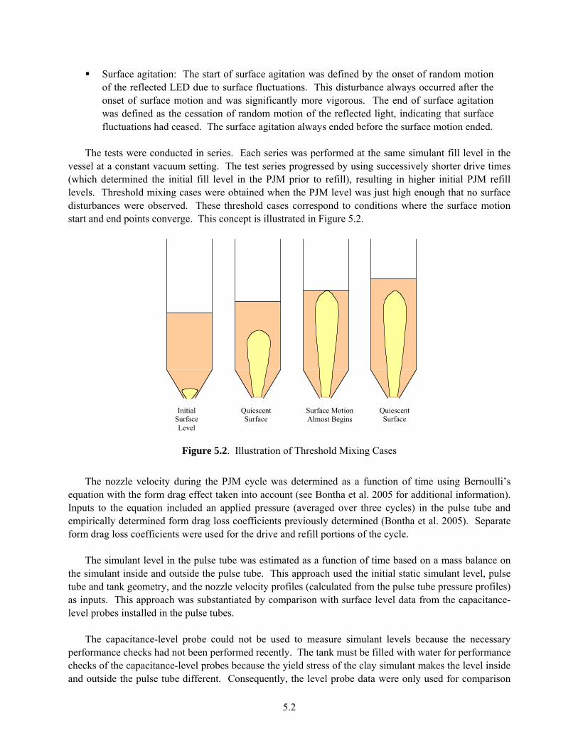
The tests were conducted in series. Each series was performed at the same simulant fill level in the vessel at a constant vacuum setting. The test series progressed by using successively shorter drive times (which determined the initial fill level in the PJM prior to refill), resulting in higher initial PJM refill levels. Threshold mixing cases were obtained when the PJM level was just high enough that no surface disturbances were observed. These threshold cases correspond to conditions where the surface motion start and end points converge. This concept is illustrated in Figure 5.2.

Initial Surface Level

Surface Motion Almost Begins

Quiescent Surface

Quiescent Surface

Figure 5.2. Illustration of Threshold Mixing Cases

The nozzle velocity during the PJM cycle was determined as a function of time using Bernoulli’s equation with the form drag effect taken into account (see Bontha et al. 2005 for additional information). Inputs to the equation included an applied pressure (averaged over three cycles) in the pulse tube and empirically determined form drag loss coefficients previously determined (Bontha et al. 2005). Separate form drag loss coefficients were used for the drive and refill portions of the cycle. The simulant level in the pulse tube was estimated as a function of time based on a mass balance on the simulant inside and outside the pulse tube. This approach used the initial static simulant level, pulse tube and tank geometry, and the nozzle velocity profiles (calculated from the pulse tube pressure profiles) as inputs. This approach was substantiated by comparison with surface level data from the capacitance-level probes installed in the pulse tubes. The capacitance-level probe could not be used to measure simulant levels because the necessary performance checks had not been performed recently. The tank must be filled with water for performance checks of the capacitance-level probes because the yield stress of the clay simulant makes the level inside and outside the pulse tube different. Consequently, the level probe data were only used for comparison

5.3

with the mass balance approach. While this comparison is for information only, the level probe data and the mass balance approach gave consistent results. The simulant level in the pulse tube and the nozzle refill velocity for the various surface agitation times were correlated with the video camera tapes by matching the start times observed for the drive or refill phases of the PJM cycle.

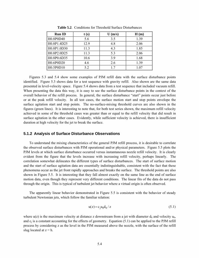
5.1.1 Observations of Surface Disturbances The video camera tests were conducted over the course of several days. Rheology measurements taken during the course of these tests indicated that the yield stress remained fairly constant at about 33 Pa. The consistency was about 24 cP. For each surface disturbance time (t) (as measured from the start of pulse tube refill) observed from the video, the corresponding PJM level (H) and nozzle velocity (U) were determined from the level and velocity refill functions. Table 5.1 summarizes these results. Table 5.2 shows the cases where no mixing was observed. These represent threshold conditions where the initial PJM level was just high enough that no surface disturbances occurred during refill. Conceptually, they approximate the conditions where surface motion start and end times converge. For these cases, the data listed in Table 5.2 correspond to the peak refill velocity conditions.

Table 5.1. Surface Disturbance Results from Video Monitoring of Pulse Tube Mixing(a)

Run ID Start Surface

Motion End Surface Motion Start Surface

Agitation End Surface

Agitation Mixing

Observed t

(s) U

(m/s) H

(m) t

(s) U

(m/s) H

(m) t

(s) U

(m/s) H

(m) t

(s) U

(m/s) H

(m) H0.8P0D50 5.9 3.7 1.04 18.4 3.4 1.36 6.3 3.7 1.05 14.6 3.5 1.26 H0.8P0D45 3.7 3.2 1.17 14.7 3.3 1.44 5.8 3.4 1.22 9.7 3.5 1.32 H0.8P1.4D35 7.8 4.7 1.58 18.6 5.0 1.96 10.4 5.0 1.67 18.3 4.9 1.95 H0.8P1.4D30 7.8 4.5 1.73 17.1 4.8 2.06 10.2 4.9 1.82 14.5 4.9 1.97 H0.8P1.0D35 9.6 4.5 1.62 19.0 4.3 1.92 11.4 4.5 1.68 15.2 4.4 1.80 H0.8P1.0D40 8.3 4.4 1.50 19.4 4.3 1.86 9.2 4.5 1.53 18.6 4.4 1.84 H0.8P2.0D30 8.5 5.2 1.79 17.5 2.0 NA(b) 12.6 5.6 1.95 14.6 4.9 2.03 H0.8P2.0D35 7.8 4.9 1.65 18.8 5.6 2.09 10.9 5.4 1.77 18.8 5.6 2.00 H0.8P0.6D55 3.2 3.5 1.02 22.8 4.1 1.61 6.1 4.1 1.10 20.1 4.1 1.53 H0.8P0.6D45 3.8 3.4 1.26 16.8 4.1 1.64 8.8 4.1 1.40 13.4 4.2 1.54 H0.6P0D30 2.2 2.6 0.83 19.5 2.6 1.19 4.2 3.0 0.87 16.1 2.7 1.12 H0.6P0D25 2.6 2.6 1.01 15.2 2.5 1.26 4.0 2.8 1.03 11.4 2.7 1.18 H0.5P0D15 2.2 1.9 0.87 16.1 1.7 1.08 4.0 2.2 0.90 10.4 1.9 1.00 H0.5P0D15-2 1.2 1.8 0.85 14.9 1.9 1.06 2.9 2.0 0.88 10.2 1.8 0.99 H0.4P0D10 1.0 1.5 0.66 14.3 1.5 0.82 5.3 1.9 0.71 7.6 1.8 0.74 (a) Refer to Figure 5.1 for a schematic showing the definitions of surface motion and surface agitation. (b) NA = not available.

5.4

Table 5.2. Conditions for Threshold Surface Disturbances

Run ID t (s) U (m/s) H (m) H0.8P0D40 5.6 3.5 1.39 H0.8P1.4D25 12.9 4.8 2.06 H0.8P1.0D30 11.3 4.3 1.85 H0.8P2.0D25 11.3 5.3 2.06 H0.8P0.6D35 10.6 3.9 1.68 H0.6P0D20 4.6 2.6 1.39 H0.5P0D10 5.2 1.7 1.07

Figures 5.3 and 5.4 show some examples of PJM refill data with the surface disturbance points identified. Figure 5.3 shows data for a test sequence with gravity refill. Also shown are the same data presented in level-velocity space. Figure 5.4 shows data from a test sequence that included vacuum refill. When presenting the data this way, it is easy to see the surface disturbance points in the context of the overall behavior of the refill process. In general, the surface disturbance “start” points occur just before or at the peak refill velocity. In all test cases, the surface motion start and stop points envelope the surface agitation start and stop points. The no-surface-mixing threshold curves are also shown in the figures (green lines). It is interesting to note that, for both test series shown, the maximum refill velocity achieved in some of the threshold cases was greater than or equal to the refill velocity that did result in surface agitation in the other cases. Evidently, while sufficient velocity is achieved, there is insufficient duration at high velocity for the jet to break the surface.

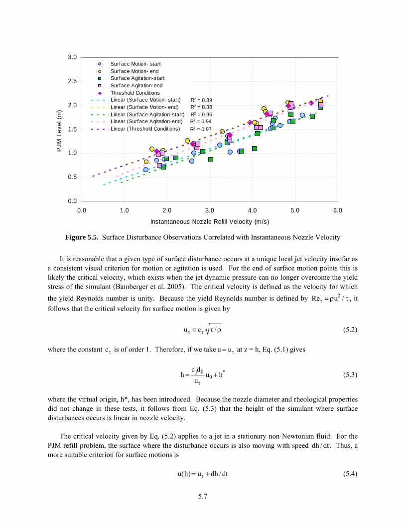
5.1.2 Analysis of Surface Disturbance Observations To understand the mixing characteristics of the general PJM refill process, it is desirable to correlate the observed surface disturbances with PJM operational and/or physical parameters. Figure 5.5 plots the PJM levels at which surface disturbance occurred versus instantaneous nozzle refill velocity. It is clearly evident from the figure that the levels increase with increasing refill velocity, perhaps linearly. The correlation somewhat delineates the different types of surface disturbances. The start of surface motion and the start of surface agitation data are essentially indistinguishable, consistent with the fact that these phenomena occur as the jet front rapidly approaches and breaks the surface. The threshold points are also shown in Figure 5.5. It is interesting that they fall almost exactly on the same line as the end of surface motion data, even though they represent very different conditions. The linear fits of the data do not pass through the origin. This is typical of turbulent jet behavior where a virtual origin is often observed. The apparently linear behavior demonstrated in Figure 5.5 is consistent with the behavior of steady turbulent Newtonian jets, which follow the familiar relation: u(z) = c ju0d0 / z (5.1)

where u(z) is the maximum velocity at distance z downstream from a jet with diameter d0 and velocity u0, and cj is a constant accounting for the effects of geometry. Equation (5.1) can be applied to the PJM refill process by considering z as the level in the PJM measured above the nozzle, with the surface of the refill slug located at z = h.

5.5

0.0

1.0

2.0

3.0

4.0

40 50 60 70 80 90 100Time (s)

Noz

zle

Ref

ill V

eloc

ity (m

/s)

1.0

1.5

2.0

2.5

PJM

Lev

el (m

)

HD0.8-P0-D50

HD0.8-P0-D45

HD0.8-P0-D40

Surface Motion

Surface Agitation

0.8

1.0

1.2

1.4

1.6

1.8

2.0 2.5 3.0 3.5 4.0

Nozzle Refill Velocity (m/s)

PJM

Lev

el (m

)

HD0.8-P0-D50

HD0.8-P0-D45

HD0.8-P0-D40

Surface Motion

Surface Agitation

Figure 5.3. Examples of Gravity-Driven PJM Refill Behavior (top, transient velocity and level refill

functions; bottom, data shown in level-velocity space)

5.6

0

1

2

3

4

5

25 30 35 40 45 50 55 60 65

Time (s)

Noz

zle

Ref

ill V

eloc

ity (m

/s)

1.0

1.5

2.0

2.5

PJM

Lev

el (m

)

HD0.8-P1.4-D35HD0.8-P1.4-D30HD0.8-P1.4-D25Surface MotionSurface Agitation

1.2

1.4

1.6

1.8

2.0

2.2

2 3 4 5 6


PJM

Lev

el (m

)

HD0.8-P1.4-D35HD0.8-P1.4-D30HD0.8-P1.4-D25Surface MotionSurface Agitation

Figure 5.4. Examples of Vacuum-Driven PJM Refill Behavior (top, transient velocity and

level refill functions; bottom, data shown in level velocity space)

5.7

R2 = 0.89

R2 = 0.95R2 = 0.88

R2 = 0.94R2 = 0.97

0.0

0.5

1.0

1.5

2.0

2.5

3.0

0.0 1.0 2.0 3.0 4.0 5.0 6.0

Instantaneous Nozzle Refill Velocity (m/s)

PJM

Lev

el (m

)Surface Motion- startSurface Motion- endSurface Agitation-startSurface Agitation-endThreshold ConditionsLinear (Surface Motion- start)Linear (Surface Motion- end)Linear (Surface Agitation-start)Linear (Surface Agitation-end)Linear (Threshold Conditions)

Figure 5.5. Surface Disturbance Observations Correlated with Instantaneous Nozzle Velocity

It is reasonable that a given type of surface disturbance occurs at a unique local jet velocity insofar as a consistent visual criterion for motion or agitation is used. For the end of surface motion points this is likely the critical velocity, which exists when the jet dynamic pressure can no longer overcome the yield stress of the simulant (Bamberger et al. 2005). The critical velocity is defined as the velocity for which the yield Reynolds number is unity. Because the yield Reynolds number is defined by Reτ = ρu2 / τ , it follows that the critical velocity for surface motion is given by uτ ≡ cτ τ / ρ (5.2) where the constant cτ is of order 1. Therefore, if we take u = uτ at z = h, Eq. (5.1) gives

h =

c jd0

uτu0 + h* (5.3)

where the virtual origin, h*, has been introduced. Because the nozzle diameter and rheological properties did not change in these tests, it follows from Eq. (5.3) that the height of the simulant where surface disturbances occurs is linear in nozzle velocity. The critical velocity given by Eq. (5.2) applies to a jet in a stationary non-Newtonian fluid. For the PJM refill problem, the surface where the disturbance occurs is also moving with speed dh / dt. Thus, a more suitable criterion for surface motions is u(h) = uτ + dh / dt (5.4)

5.8

The speed of the surface is related to the nozzle velocity by(a)

dhdt

= A0APT

u0 (5.5)

where A0 is the nozzle area and APT is the cross-sectional area of a pulse tube. By combining Eq. (5.4), (5.5), and (5.1), we obtain

h =

c jd0

uτu0 1+ A0

APT

u0uτ

⎡

⎣ ⎢

⎤

⎦ ⎥ −1

+ h* (5.6)

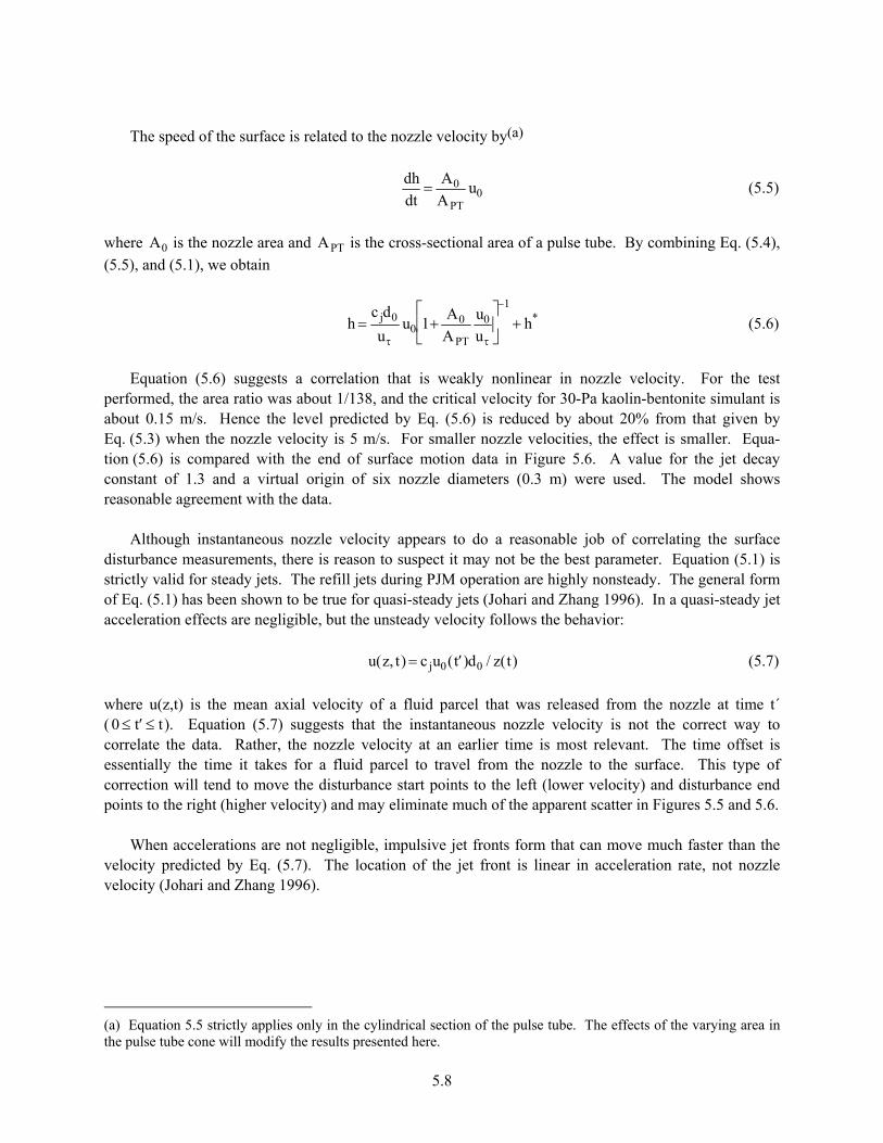
Equation (5.6) suggests a correlation that is weakly nonlinear in nozzle velocity. For the test performed, the area ratio was about 1/138, and the critical velocity for 30-Pa kaolin-bentonite simulant is about 0.15 m/s. Hence the level predicted by Eq. (5.6) is reduced by about 20% from that given by Eq. (5.3) when the nozzle velocity is 5 m/s. For smaller nozzle velocities, the effect is smaller. Equa-tion (5.6) is compared with the end of surface motion data in Figure 5.6. A value for the jet decay constant of 1.3 and a virtual origin of six nozzle diameters (0.3 m) were used. The model shows reasonable agreement with the data. Although instantaneous nozzle velocity appears to do a reasonable job of correlating the surface disturbance measurements, there is reason to suspect it may not be the best parameter. Equation (5.1) is strictly valid for steady jets. The refill jets during PJM operation are highly nonsteady. The general form of Eq. (5.1) has been shown to be true for quasi-steady jets (Johari and Zhang 1996). In a quasi-steady jet acceleration effects are negligible, but the unsteady velocity follows the behavior: u(z, t) = c ju0( ′ t )d0 / z(t) (5.7) where u(z,t) is the mean axial velocity of a fluid parcel that was released from the nozzle at time t´ ( 0 ≤ ′ t ≤ t). Equation (5.7) suggests that the instantaneous nozzle velocity is not the correct way to correlate the data. Rather, the nozzle velocity at an earlier time is most relevant. The time offset is essentially the time it takes for a fluid parcel to travel from the nozzle to the surface. This type of correction will tend to move the disturbance start points to the left (lower velocity) and disturbance end points to the right (higher velocity) and may eliminate much of the apparent scatter in Figures 5.5 and 5.6. When accelerations are not negligible, impulsive jet fronts form that can move much faster than the velocity predicted by Eq. (5.7). The location of the jet front is linear in acceleration rate, not nozzle velocity (Johari and Zhang 1996).

(a) Equation 5.5 strictly applies only in the cylindrical section of the pulse tube. The effects of the varying area in the pulse tube cone will modify the results presented here.

5.9

R2 = 0.946

0.0

0.5

1.0

1.5

2.0

2.5

0.0 1.0 2.0 3.0 4.0 5.0 6.0 7.0Instantaneous Nozzle Refill Velocity (m/s)

PJM

Lev

el (m

)

Surface Motion- end

Model

Linear (Surface Motion- end)

R2=0.943

Figure 5.6. Comparing End of Surface Motion Data with Nonlinear Model

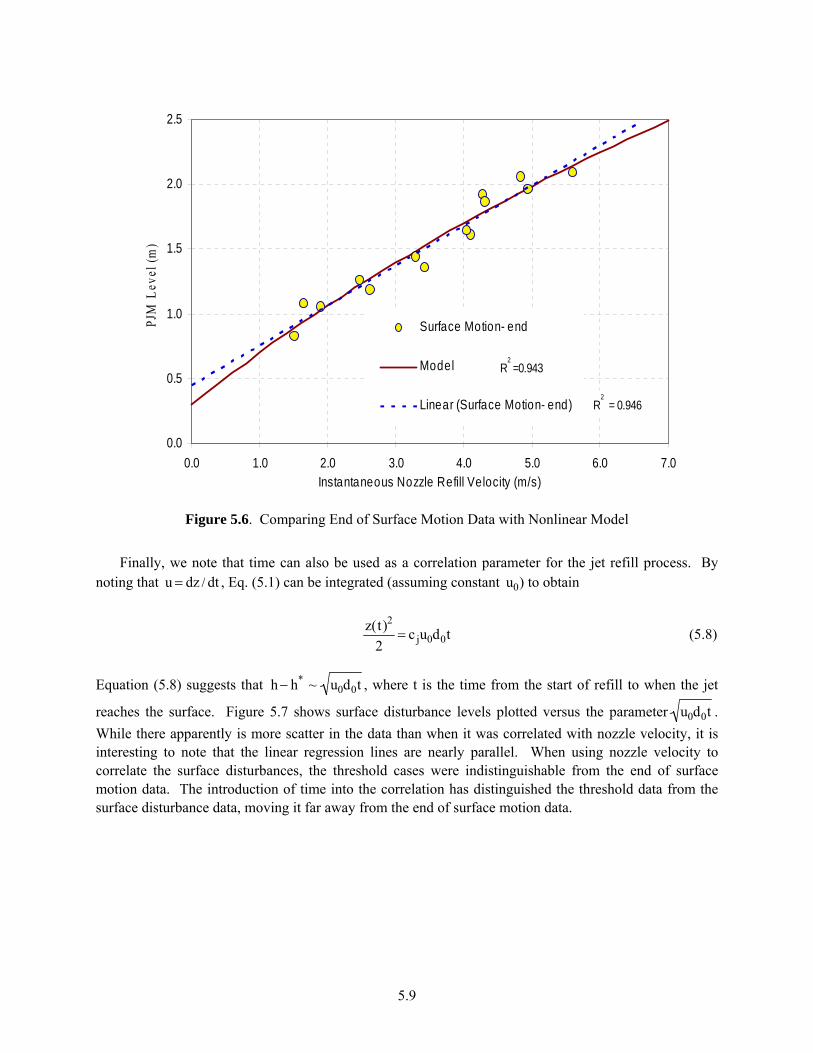
Finally, we note that time can also be used as a correlation parameter for the jet refill process. By noting that u = dz / dt , Eq. (5.1) can be integrated (assuming constant u0) to obtain

z(t)2

2= c ju0d0t (5.8)

Equation (5.8) suggests that h − h* ~ u0d0t , where t is the time from the start of refill to when the jet

reaches the surface. Figure 5.7 shows surface disturbance levels plotted versus the parameter u0d0t . While there apparently is more scatter in the data than when it was correlated with nozzle velocity, it is interesting to note that the linear regression lines are nearly parallel. When using nozzle velocity to correlate the surface disturbances, the threshold cases were indistinguishable from the end of surface motion data. The introduction of time into the correlation has distinguished the threshold data from the surface disturbance data, moving it far away from the end of surface motion data.

5.10

R2

= 0.91R

2 = 0.86

R2

= 0.93R

2 = 0.85

R2

= 0.990.0

0.5

1.0

1.5

2.0

2.5

0.0 0.5 1.0 1.5 2.0 2.5 3.0

(u0d0t)1 / 2

PJM

Lev

el (m

)

Surface Motion- startSurface Motion- endSurface Agitation-startSurface Agitation-endThreshold ConditionsLinear (Surface Motion- start)Linear (Surface Motion- end)Linear (Surface Agitation-start)Linear (Surface Agitation-end)Linear (Threshold Conditions)

Figure 5.7. Surface Disturbance Observations Correlated with the Parameter u0d0t

5.2 Pulse Tube Tracer Mixing Test: Half-Stroke

5.2.1 Mixing Test Approach: Half-Stroke The various testing runs in the pulse tube tracer mixing test are presented in Table 5.3 along with the objectives, target operating conditions, and sampling protocol. The test began with Run 1 by mixing the tank contents with the PJMs operating at full stroke and the main spargers operating at a nominal air flow rate of 18.8 ±2 acfm at the nozzle. The simulant rheology was checked and adjusted by dilution to be within the target yield stress of 30 ±5 Pa. At this point, initial samples were taken from three grab sampling locations in the tank. After the samples were collected, the tank and its contents were left undisturbed (except for standby sparger air flow) for a period of ~15.5 hours. Run 2 was conducted with the spargers and PJM #7 off by putting the pulse tube in the vent mode, with the other seven PJMs operating at half stroke. The air spargers were not used again until the final run. With seven PJMs operating at half stroke the tracer solution was introduced into the tank, as discussed in Section 4.3.2. Once the tracer injection was completed, mixing with the seven PJMs continued for a total of 2 hours to homogenize the salt tracer within the PJM cavern. Grab samples were collected from the three sample locations using the approach discussed in Section 4.3.3.

5.11

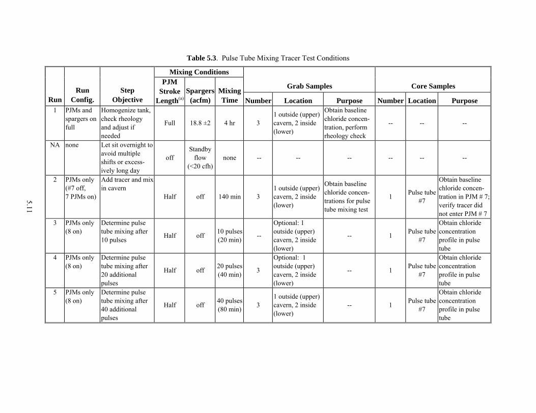
Table 5.3. Pulse Tube Mixing Tracer Test Conditions

Mixing Conditions

Grab Samples Core Samples

Run Run

Config. Step

Objective

PJM Stroke

Length(a)Spargers

(acfm) Mixing Time Number Location Purpose Number Location Purpose

1 PJMs and spargers on full

Homogenize tank, check rheology and adjust if needed

Full 18.8 ±2 4 hr 3 1 outside (upper) cavern, 2 inside (lower)

Obtain baseline chloride concen-tration, perform rheology check

-- -- --

NA none Let sit overnight to avoid multiple shifts or excess-ively long day

off Standby

flow (<20 cfh)

none -- -- -- -- -- --

2 PJMs only (#7 off, 7 PJMs on)

Add tracer and mix in cavern

Half off 140 min 3 1 outside (upper) cavern, 2 inside (lower)

Obtain baseline chloride concen-trations for pulse tube mixing test

1 Pulse tube #7

Obtain baseline chloride concen-tration in PJM # 7; verify tracer did not enter PJM # 7

3 PJMs only (8 on)

Determine pulse tube mixing after 10 pulses Half off 10 pulses

(20 min) --

Optional: 1 outside (upper) cavern, 2 inside (lower)

-- 1 Pulse tube #7

Obtain chloride concentration profile in pulse tube

4 PJMs only (8 on)

Determine pulse tube mixing after 20 additional pulses

Half off 20 pulses (40 min) 3

Optional: 1 outside (upper) cavern, 2 inside (lower)

-- 1 Pulse tube #7


5 PJMs only (8 on)



1 outside (upper) cavern, 2 inside (lower)

-- 1 Pulse tube #7


5.12

Table 5.3 (contd)

Mixing Conditions Grab Samples Core Samples

Run Run

Config. Step

Objective

PJM Stroke

Length(a)Spargers


6 PJMs only (8 on)




Estimate cavern size, determine cavern rheology

1 Pulse tube #7, #3

Obtain chloride concentration profile in pulse tube and cavern size with PJMs at half stroke. Compare core sample results to assess the impact of repeated coring of PJM # 7

7 PJMs only (8 on)

Approach uniform cavern concentration Full off 160 min 3


Estimate cavern size, determine cavern rheology

2 Pulse tube #2, #6

Determine cavern size and mixing in pulse tube and verify mixing in pulse tubes operating at full stroke


Homogenize tank for final sampling

Full 18.8 ±2 3 hr 3 1 outside (upper) cavern, 2 inside (lower)

Obtain final concentration for mass balance, obtain final rheology values

1 Pulse tube #7

Provide homogenized tracer concentration for mass balance and confirm mixing at full stroke.

(a) Target PJM peak average nozzle velocity: 11.5 ±0.5 m/s. PJM cycle time for half-stroke operation: 120 sec. PJM cycle time for full-stroke operation: ~150 sec.

5.13

In addition, an initial core sample was taken from PJM #7. Runs 3 to 6 involved operating all of the PJMs at half-stroke with sampling events taking place after 10, 30, 70, and 150 total cycles. A core sample was obtained from PJM #7 after each set of cycles. Grab samples were also taken but were generally not analyzed for chloride concentration. At the end of the 150 cycles, a core sample was also obtained from PJM #3. By comparing the results of the core samples from PJMs #7 and #3 (which had not been sampled previously), it was possible to assess the effect of the core sampling process on the chloride distribution. After the half-stroke test, the PJMs were operated at full stroke for 60 additional cycles (2 hr) and final core samples were collected from PJMs #2 and #6 to verify that mixing of the pulse tube contents is achieved by operation at full stroke. Grab samples were also obtained in order to estimate the mixing cavern size. Unfortunately, a plug in the air supply pipe above PJM #4 prevented the pulse tube from completely filling. This led to an overblow of PJM #4 on the subsequent cycle (cycle 28 of Run 7). The overblow disrupted the cavern and affected this portion of the test. The final run involved homogenization of the simulant with the PJMs at full stroke and the spargers on full-flow (18.8 ±2 acfm) for 3 hours. After homogenizing the tank, a final core sample from PJM #7 and grab samples from the tank were collected. The PJM drive functions for the half-stroke and full-stroke tests are shown in Figure 5.8. These are averaged from multiple tubes. The half-stroke drive function had a maximum refill velocity of 2.6 m/s and an initial PJM level of 1.57 m (62 inches) at the start of the refill phase. The full-stroke drive function had a maximum refill velocity of 3.7 m/s and an initial PJM level of 0.66 m (26 inches) at the start of the refill phase. The maximum PJM level for both drive functions was approximately 2.46 m (97 inches) and occurred at the start of each drive. The cycle time for full-stroke operation was extended from 120 to ~150 seconds to accommodate the relatively long refill time. The terms full stroke and half stroke have typically been used to describe PJM operation. The volume of the pulse tube contents expelled during a full-stroke drive typically ranges from 80–90% of the pulse tube volume. For quantitative purposes in this report, we define a full stroke as a stroke length sufficient to expel 85% of the volume of the pulse tube. A half stroke is defined as one half of a full stroke or a stroke length sufficient to expel 42.5% of the pulse tube volume. Because the PJMs in the full-scale WTP are designed to always fill to the top of the pulse tube, the percent of theoretical full stroke is defined by the slurry level in the PJM at the end of the drive period. Figure 5.9 illustrates this, plotting the percent of volume and percent of full stroke versus the level at the end of a drive period (initial refill level) for the HSLS pulse tubes. As shown in Table 5.4, the equivalent half-stroke and full-stroke test conditions exceeded the target volumes (compare columns 1 and 2 with 4 and 5) based on the level at the end of the drive period. During the tracer test, the vacuum applied to the system during refill was reduced to provide a minimum nozzle refill velocity. This vacuum was not quite enough to refill the pulse tubes, so each drive began about 18 inches below the top of the pulse tube, causing the drive phase (start of refill) for half-stroke operation to end at a level approximately 8 inches below that of an ideal half-stroke drive.(a) The simulant

(a) In this case, ideal refers to a drive starting at the top of the pulse tube.

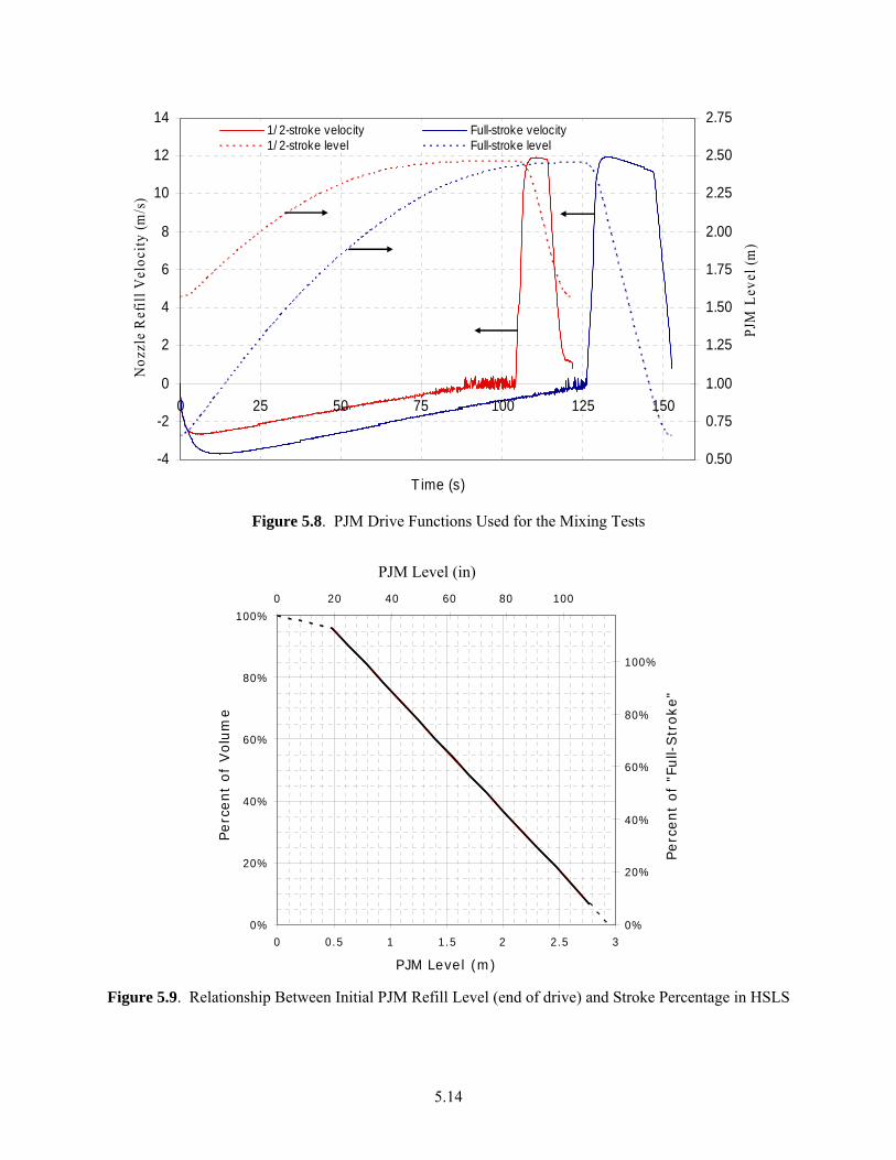
5.14

-4

-2

0

2

4

6

8

10

12

14

0 25 50 75 100 125 150

Time (s)

Noz

zle

Ref

ill V

eloc

ity (m

/s)

0.50

0.75

1.00

1.25

1.50

1.75

2.00

2.25

2.50

2.75

PJM

Lev

el (m

)

1/ 2-stroke velocity Full-stroke velocity1/ 2-stroke level Full-stroke level

Figure 5.8. PJM Drive Functions Used for the Mixing Tests

0%

20%

40%

60%

80%

100%

0 0.5 1 1.5 2 2.5 3

PJM Level (m)

Perc

ent

of

Volu

me

0%

20%

40%

60%

80%

100%

0 20 40 60 80 100

Perc

ent

of

"Full-

Str

oke"

Figure 5.9. Relationship Between Initial PJM Refill Level (end of drive) and Stroke Percentage in HSLS

PJM Level (in)

5.15

Table 5.4. PJM Stroke Characteristics Achieved in the Tracer Mixing Test

Target Conditions(a) Equivalent Test Conditions(a) Actual Stroke Tested(b)

Stroke Half stroke Full stroke Half stroke Full stroke Half stroke Full strokePercent of PJM volume

42.5 85 51 86 35 70

Percent of full stroke

50 100 60 102 41 83

(a) Stroke calculated assuming refill to top of pulse tube. (b) Stroke calculated from actual level change in the pulse tube.

level at the end of the drive phase for full-stroke operation was only 1 inch below the ending level of an ideal full-stroke drive (see appendix for a detailed description of stroke lengths and simulant levels during the test). Therefore, based on an assumed fill level to the top of the pulse tube, the effective test stroke length was greater than the target, more so for half-stroke than full stroke. As shown in Table 5.4, the half-stroke and full-stroke test conditions expelled less than the target volume of simulant (columns 4 and 5) during each PJM cycle. This is an important consideration for analyzing cavern size (% mixed). The last two columns show that the effective stroke length for the purpose of refill was greater than the target. This is because the simulant level at the end of the drive phase was lower than the target level. The fact that the actual drive stroke length was somewhat reduced due to incomplete filling of the pulse tube is considered inconsequential for refill mixing analysis. The impact of the effective refill stroke length is accounted for in the estimate of the stroke length required for complete mixing of the pulse tube contents (see Section 5.4). The yield stress of the clay during the test is shown as a function of the number of PJM cycles in Figure 5.10. The addition of the salt tracer increases the interactions between the clay particles, which leads to a slight increase in yield stress.

3333.5

3434.5

3535.5

3636.5

3737.5

38

0 100 200 300 400

PJM Cycles

Yie

ld S

tress

(Pa)

Tracer Added

end of test

All PJMs at half-stroke

All PJMs at Full stroke

PJMs at full-stroke + spargers on full flow

Figure 5.10. Yield Stress of Simulant During the Tracer Test

5.16

Even though the defined effective stroke lengths were greater than target values, the half- and full-stroke test conditions actually expelled less than the target volume of simulant during each PJM cycle due to incomplete filling of the pulse tubes (see last two columns of Table 5.4). Though this is an important consideration for analyzing cavern size (% mixed), incomplete filling of pulse tubes is inconsequential for refill mixing analysis. The effect of the reduced actual refill stroke length is accounted for in the estimate of the stroke length required for complete mixing of the pulse tube contents (see Section 5.4). Core sample results for the runs during the tracer mixing test are shown sequentially from start to finish in Figures 5.11 to 5.17. In each figure, the depth of the core segment is plotted with the chloride concentration. Zero depth corresponds to the top of the simulant in the pulse tube, while the bottom sample at about 55 inches was near the bottom of the pulse tube. The core segment depth has been adjusted for core compression using the information presented in Section 4.3.4. For comparison, the initial baseline chloride concentration of 139 ppm is shown.(a) This concentration is based on analysis of grab samples taken before the tracer was added. In most plots the chloride concentration of the top core segment at a depth of 1.5 inches is lower than the initial baseline chloride concentration. This is thought to be due to water dilution of the top 3-inch segment in the core. The dilution has two possible sources. One possibility is that the water originated from the core sampling tubes, which were wetted prior to insertion into the pulse tube in an effort to minimize core compression. As the sample was pushed up into the tube its possible that water droplets adhering to the inner tube wall were collected at the top of the sample. When the top 3-inch segment was composited for analysis the extra water diluted the sample. The other possibility is that condensation of water from the air driving the pulse tubes collected on top of the simulant slug inside of the pulse tube. During the video camera work, drops of water were often observed falling onto the top of the simulant.

0

12

24

36

48

60

100

120

140

160

180

200

220

Cl-, ppm

Cor

e S

egm

ent D

epth

(inc

hes)

InitialConc.Run 2;PJM 7

Figure 5.11. Core Sample Results for Run 2 (initial baseline concentration in PJM #7)

a The initial concentration is based on the average concentration determined from the 3 initial grab samples obtained prior to the addition of the tracer.

5.17

The initial core sample taken at the end of Run 2 (Figure 5.11) shows that little if any tracer was drawn into PJM #7. This PJM was in vent mode and was not operating during Run 2 when the tracer was added to the mixing cavern. As shown in Figures 5.12 through 5.15, the tracer concentration profile was rapidly established during the half-stroke operation and exhibited only modest changes over the 150 cycles at half stroke. The core sample taken from PJM #7 after 10 cycles at half stroke (Figure 5.12, Run 3) shows that the chloride tracer had mixed into most of the lower portion of the simulant in the pulse tube. The top 25.5 inches of the core sample exhibited a rapidly decreasing chloride concentration. This general profile is maintained through the next set of core samples taken after 30, 70, and 150 cycles at half stroke. The chloride con-centration profile in the lower portion of the core samples was reasonably constant, indicating uniform mixing in this region. The chloride concentration dropped to near the initial baseline over a span of about 6 inches. The core samples taken after 150 cycles indicate that the mixing interface increased by about 3 inches, from 25.5 (Runs 3, 4, 5) to 22.5 inches from the top of the simulant (Run 6, Figure 5.15). After Run 6 (150 cycles) a different pulse tube (#3) was also core sampled for comparison with results from PJM #7. As shown in Figure 5.15, results from both core samples are fairly consistent. This indicates that the repeated core sampling of PJM #7 had a negligible effect on the results. The concern was that the core sampling process would entrain tracer into the unmixed portion of the simulant in the upper part of the pulse tube. Run 7 involved running the PJMs at full stroke for 60 cycles. As shown in Figure 5.16, the tracer concentration profile indicates that the entire contents of the pulse tube were being mixed during refill. Run 8 (Figure 5.17) involved running the PJMs at full stroke with the spargers operating for 3 hours to homogenize tank contents. Final grab samples from the tank indicate an average chloride concentration of 177 ppm; the final core sample from PJM #7 indicates a concentration slightly greater than 180 ppm.

0

12

24

36

48

60

100

120

140

160

180

200

220

Cl-, ppm

Cor

e S

egm

ent D

epth

(inc

hes)

InitialConc.

Run 3;PJM 7

Figure 5.12. Core Sample Results for Run 3 (sample taken from PJM #7 after 10 cycles at half stroke)

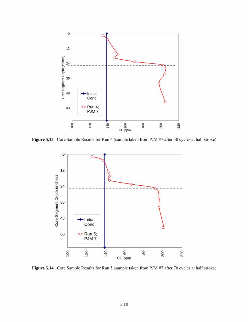
5.18

0

12

24

36

48

60

100

120

140

160

180

200

220

Cl-, ppm

Cor

e S

egm

ent D

epth

(inc

hes)

InitialConc.

Run 4;PJM 7


0

12

24

36

48

60

100

120

140

160

180

200

220

Cl-, ppm

Cor

e S

egm

ent D

epth

(inc

hes)

InitialConc.

Run 5;PJM 7


5.19

0

12

24

36

48

60

100

120

140

160

180

200

220

Cl-, ppm

Cor

e S

egm

ent D

epth

(inc

hes)

InitialConc.GrabSamplesRun 6;PJM 7Run 6;PJM 3

Figure 5.15. Core Sample Results for Run 6 (samples taken from PJMs #3 and #6 after 150 cycles

at half stroke)(a)

0

12

24

36

48

60

100

120

140

160

180

200

220

Cl-, ppm

Cor

e S

egm

ent D

epth

(inc

hes)

InitialConc.

GrabSamples

Run 7;PJM 6

Run 7;PJM 2

Figure 5.16. Core Sample Results for Run 7 (samples taken from PJMs 2 and 6 after 60 cycles

at full stroke) a The initial concentration is based on the average concentration determined from the 3 initial grab samples obtained prior to the addition of the tracer. The grab sample concentration is the final average concentration determined from grab samples obtained after complete homogenization of the clay simulant.

5.20

0

12

24

36

48

60

100

120

140

160

180

200

220

Cl-, ppm

Cor

e S

egm

ent D

epth

(inc

hes)

InitialConc.

GrabSamples

Run 8;PJM 7

Figure 5.17. Core Sample Results for Run 8 (samples taken from PJM 7 after 3 hours of

mixing with PJMs operating at full stroke and spargers operating at full flow)

Table 5.5 shows the fraction of the HSLS vessel mixed (percent mixed values) based on the core sample results for Runs 3-6. The salt concentrations from the lower portions of the core samples were assumed equivalent to the concentrations in the mixing cavern. The percent mixed values were determined using the method presented by Poloski et al. (2004b) and indicate the fraction of the clay simulant in the vessel that was mixed by the pulse tubes operating at half stroke. The percent mixed value for Run 7 (operation at full stroke) was also determined to be 76%. This value may be somewhat high because of an inadvertent overblow of one of the pulse tubes during the full-stroke operation that provided additional mixing.

Table 5.5. Percent Mixed Values for Operation at Half Stroke

Run # Total Number of half strokes Percent mixed (%) 3 10 65 4 30 60 5 70 65 6 150 68

5.3 Comparison of Video Camera Results and Tracer Results In this section, an effort is made to compare the results of the tracer mixing tests with the video surface disturbance observations. The goal is to relate and interpret the surface disturbances (i.e., start of

5.21

agitation, etc.) to the location of the mixing interface determined by the tracer mixing test. If this relationship can be established, then the video surface disturbance data can be used to evaluate the mixing performance for a broad range of operating conditions. The PJM refill velocity and level curves used in the two mixing tracer tests are shown in Figure 5.18. It is reasonable to assume that the half-stroke mixing interface identified from the core analysis translated up and down with the same velocity-time history as the surface of the slug. Core sampling found the position of the mixing interface to be 22.5 inches below the surface of the slug. Hence, by subtracting 22.5 inches from the half-stroke level curve, the elevation and velocity variation of the mixing interface with time can be found. This mixing interface trajectory is also shown in Figure 5.18.

0

1

2

3

4

0 20 40 60 80 100

Time (s)

Noz

zle

Ref

ill V

eloc

ity (m

/s)

0.0

0.5

1.0

1.5

2.0

2.5

3.0

PJM

leve

l (m

)

1/2-stroke mixing test

full-stroke mixing test

1/2-stroke mixing interface

0.0

0.5

1.0

1.5

2.0

2.5

3.0

0.0 0.5 1.0 1.5 2.0 2.5 3.0 3.5 4.0


PJM

Lev

el (m

)

full-stroke mixing test1/2-stroke mixing test1/2-stroke mixing interface

Figure 5.18. Refill Velocity and Level Used in the Mixing Tracer Tests (top). Also shown is the

trajectory of the mixing interface for the half-stroke mixing test (bottom).

5.22

In Figure 5.19, the mixing test refill functions and interface trajectory are shown with video surface disturbance data. Several points are evident when comparing the data. First, the surface level of the half-stroke mixing test (red curve) remains well above the surface disturbance data, consistent with the observation that the entire slug did not mix. At each elevation along the refill trajectory, the refill velocity is less than that determined from the video data. The surface level for the full-stroke mixing test (blue curve) clearly crosses the video data, consistent with complete mixing in the test. For much of the trajectory, velocity conditions are capable of surface disruptions at elevations that exceed that of the slug. The mixing interface trajectory (green line in Figure 5.19) crosses partway into the video data cluster, suggesting that video surface disturbance data are indeed related to actual mixing. The trajectory crosses the mixing and agitation “end” lines but only approaches the “start” lines. However, it is not clear at which point on the trajectory the jet actually reached the mixing interface. Because precise location on the trajectory where mixing occurred is not known, there is no way to identify from the figure which surface disturbance type is most closely associated with actual mixing.

0.0

0.5

1.0

1.5

2.0

2.5

0.0 1.0 2.0 3.0 4.0 5.0 6.0 7.0


PJM

Lev

el (m

)

Surface Motion- startSurface Motion- endSurface Agitation-startSurface Agitation-f inish1/2 Stoke Mixing Test1/2 Stroke Mixing InterfaceFull Stroke Mixing Test

Figure 5.19. Mixing Test Refill Curves Compared with Video Surface Disturbance Data:

Instantaneous Nozzle Velocity Correlation

To aid in understanding the relationship between observed surface disturbance and mixing, Figure 5.20 presents the data correlated with the time parameter u0d0t . When the data are presented this way, the mixing interface curve first crosses the start of surface motion line, then progresses farther through the start of surface agitation to the end of surface agitation. The trajectory finally just touches the end of the surface motion line. While it is still not clear at what point mixing occurred, it follows that mixing must have occurred by the time the interface reached the end of the surface agitation line. It is evident in Figure 5.19 that the trajectory crossed the end of the surface agitation line from below. If the trajectory had crossed the line from above, it is likely that mixing would not have occurred. Thus, a rea-sonable interpretation is that the end of surface agitation data represents conditions where mixing occurs insofar as the trajectory approaches those conditions from below (on a level-velocity correlation).

5.23

0.0

0.5

1.0

1.5

2.0

2.5

0.0 0.5 1.0 1.5 2.0 2.5 3.0

(u0d0t)1 / 2

PJM

Lev

el (m

)

Surface Motion- startSurface Motion- endSurface Agitation-startSurface Agitation-finish1/2 Stroke Mixing Test1/2 Stroke Mixing InterfaceFull Stroke Mixing Test

Figure 5.20. Mixing Test Refill Curves Compared with Video Surface Disturbance Data:

Time Parameter Correlation

Figure 5.21 shows linear fits of the start and end of surface motion data, together with the mixing interface trajectory. The solid blue line in Figure 5.21 is the start of surface motion line translated upward so that the mixing trajectory intercepts it. This line is a reasonable representation for the velocity required for a slug of simulant of height h to be mixed during refill. The equation for the line is given by h = 0.3u0 + 0.25 (5.9)

5.4 Interpretation and Application of Results Relating the video surface disturbance to the tracer mixing test results provides a useful means to evaluate the effect of stroke length on mixing inside the pulse tube. Figure 5.22 demonstrates a refill mixing performance map constructed from the test data. The “threshold of mixing” line shown in Figure 5.22 divides the level-velocity plane into two segments. PJM trajectories that cross the line from left to right will result in complete mixing of the simulant slug inside the PJM. Trajectories that do not cross the line will not provide complete mixing. Trajectories that just touch the line are barely sufficient to mix the pulse tube contents. The information contained in Figure 5.22 can be cast in terms of percent stroke by using the geometric relationship between the minimum pulse tube level and volume assuming complete refill (see Figure 5.9). Figure 5.23 shows a PJM stroke- velocity map. On the left-hand axis, the level is converted to percent of full stroke. As mentioned previously, full stroke is defined as 85% of the total PJM volume. When plotted this way, trajectories that touch or cross the mixing threshold line exhibit complete mixing of pulse tube contents.

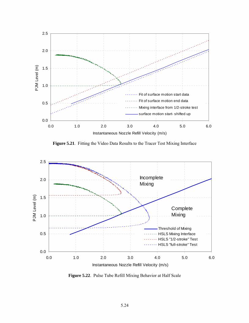
5.24

0.0

0.5

1.0

1.5

2.0

2.5

0.0 1.0 2.0 3.0 4.0 5.0 6.0


PJM

Lev

el (m

)

Fit of surface motion start data

Fit of surface motion end data

Mixing interface from 1/2-stroke test

surface motion start- shifted up

Figure 5.21. Fitting the Video Data Results to the Tracer Test Mixing Interface

0.0

0.5

1.0

1.5

2.0

2.5

0.0 1.0 2.0 3.0 4.0 5.0 6.0


PJM

Lev

el (m

)

Threshold of MixingHSLS Mixing InterfaceHSLS "1/2-stroke" TestHSLS "full-stroke" Test

IncompleteMixing

Complete Mixing

Figure 5.22. Pulse Tube Refill Mixing Behavior at Half Scale

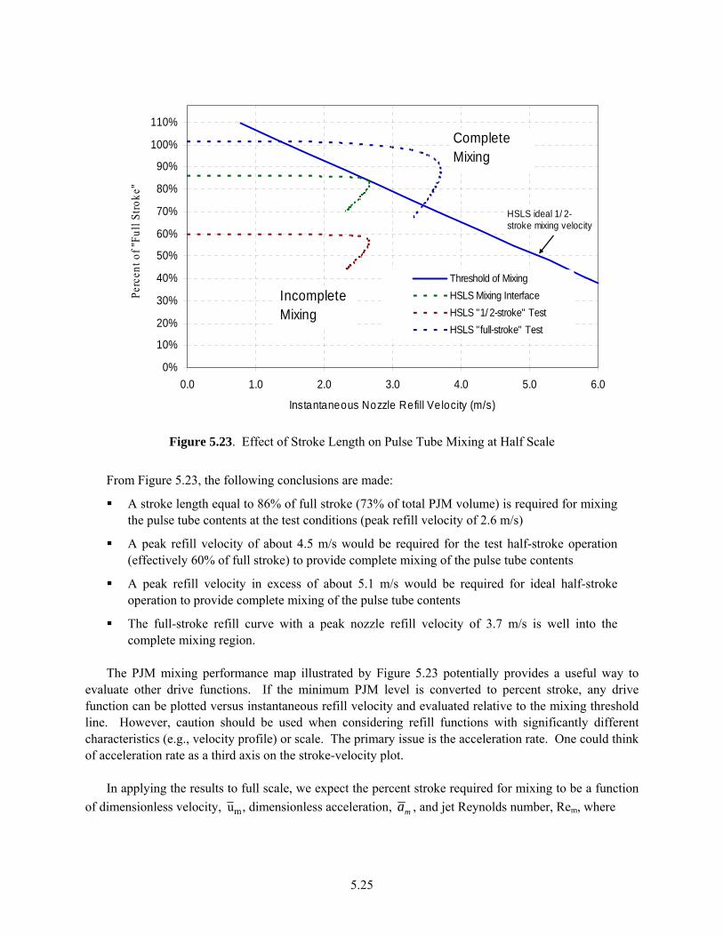
5.25

0%

10%

20%

30%

40%

50%

60%

70%

80%

90%

100%

110%

0.0 1.0 2.0 3.0 4.0 5.0 6.0


Perc

ent o

f "Fu

ll St

roke

"

Threshold of MixingHSLS Mixing InterfaceHSLS "1/ 2-stroke" TestHSLS "full-stroke" Test

CompleteMixing

Incomplete Mixing

HSLS ideal 1/ 2-stroke mixing velocity

Figure 5.23. Effect of Stroke Length on Pulse Tube Mixing at Half Scale

From Figure 5.23, the following conclusions are made:

A stroke length equal to 86% of full stroke (73% of total PJM volume) is required for mixing the pulse tube contents at the test conditions (peak refill velocity of 2.6 m/s)

A peak refill velocity of about 4.5 m/s would be required for the test half-stroke operation (effectively 60% of full stroke) to provide complete mixing of the pulse tube contents

A peak refill velocity in excess of about 5.1 m/s would be required for ideal half-stroke operation to provide complete mixing of the pulse tube contents

The full-stroke refill curve with a peak nozzle refill velocity of 3.7 m/s is well into the complete mixing region.

The PJM mixing performance map illustrated by Figure 5.23 potentially provides a useful way to evaluate other drive functions. If the minimum PJM level is converted to percent stroke, any drive function can be plotted versus instantaneous refill velocity and evaluated relative to the mixing threshold line. However, caution should be used when considering refill functions with significantly different characteristics (e.g., velocity profile) or scale. The primary issue is the acceleration rate. One could think of acceleration rate as a third axis on the stroke-velocity plot. In applying the results to full scale, we expect the percent stroke required for mixing to be a function of dimensionless velocity, u m, dimensionless acceleration, ma , and jet Reynolds number, Rem, where

5.26

τu

uum

max= (5.10)

2max

0max

udaam = (5.11)

κ

ρ 0maxRedu

m = (5.12)

u max and a max are the maximum refill velocity and acceleration, respectively. Note that given the

definition of the critical velocity, (Eq. 5.2) τu is proportional to Reτ1/2.

To apply these results to assess the full-scale (i.e. plant scale) mixing behavior in a pulse tube, additional information is needed, along with either additional testing at different scales or analysis using an appropriate computational fluid dynamics (CFD) model. Full-scale refill functions will be needed for an estimate of the dimensionless parameters in Eq. (5.10) through (5.12). If the dimensionless acceleration and velocity at full scale is greater than or equal to the values at half-scale, we expect the mixing results obtained at half scale to be conservative because the jet Reynolds number will be larger at full-scale; mixing is expected to improve as the jet Reynolds number increases. However, if the dimensionless acceleration of the full-scale refill function is smaller than at half scale, it is possible that the test results could be nonconservative. The location of the mixing line (see Figures 5.22 and 5.23) will also need to be estimated at full scale. This may be obtained by additional pulse tube mixing tests at different scales. Alternatively, it may be possible to estimate the location of the mixing line using an appropriate CFD model.

6.1

6.0 Pulse Tube Tracer Mixing Test: Full Stroke Table 6.1 presents the various testing runs in the full-stroke pulse tube tracer mixing test along with the objectives, target operating conditions, and sampling protocol. The test began with Run 1 by mixing the tank contents with the PJMs operating at full stroke and the main spargers operating at a nominal air flow rate of 18.8 ±2 acfm at the nozzle. The simulant rheology was checked and confirmed to be within the target yield stress of 30 ± 5 Pa. At this point, initial samples were taken from three grab sampling locations in the tank. After the samples were collected, the tank and its contents were left undisturbed (except for standby sparger air flow) for ~24.5 hours. Run 2 was conducted with the spargers and PJM #6 off, by putting that pulse tube in the vent mode, with the other seven PJMs operating at full-stroke equivalent. The air spargers were not used again until the final run. With seven PJMs operating at full-stroke equivalent, the tracer solution was introduced into the tank, as discussed in Section 4.3.2. Once the tracer injection was completed, mixing with the seven PJMs continued for an additional 2.5 hours to homogenize the salt tracer within the PJM cavern. An initial core sample was taken from the center location of PJM #6. Runs 3 to 8 involved operating all of the PJMs at full-stroke equivalent with core sampling events taking place after 1, 2, 3, 4, 5, and 10 total cycles at full-stroke equivalent. The final run involved homogenization of the simulant with the PJMs at full stroke and the spargers on full flow (18.8 ±2 acfm) for 3 hours. After homogenizing the tank, three grab samples were collected from the tank. Figure 6.1 shows the approximate PJM refill velocity profile for the full-stroke equivalent test. This profile is derived from the video camera testing described in Section 5. The specific run ID is H0.6P0D30. The pulse tube refill conditions for this video camera test were nearly identical to the full-stoke equivalent refill conditions. Also shown in the plot is the line that approximately represents the boundary between complete mixing and incomplete mixing of the pulse tube contents (refer to Section 5.4). The refill velocity curve extends well into the complete mixing region, indicating that the mixing of the pulse tube contents is expected. Runs 2 to 8 used what is termed a full-stroke equivalent. A full-stroke equivalent ended at a level in the pulse tube that corresponds to expelling 80% of the pulse tube volume. Because the stroke started with the level in the pulse tube at roughly the static level in the tank (H/D ~ 0.57), the actual volume expelled during the drive is less than a full-stroke volume, but it was the simulant level at the start of the refill that was important for this test. This level is somewhat higher in the pulse tube than the level for a full stroke, which is based on expelling 85% of the pulse tube contents. The 80% was chosen to add an element of conservatism in that the amount of material that needed to be mixed during refill is the maximum amount given that the volume expelled during a full stroke ranges from 80 to 90% of the pulse tube volume. Figure A.5 in the appendix provides a detailed description of stroke length and simulant levels during the test.

6.2

Table 6.1. Pulse Tube Mixing Tracer Test Conditions


Run Run

Config. Step

Objective

PJM Stroke

Length(a)Spargers



Homogenize tank, check rheology, and adjust if needed

Full 18.8 ±2 2 hr 3 1 upper region, 2 lower region

Obtain baseline chloride concen-tration, perform rheology check

-- -- --

NA none

Let sit overnight to avoid multiple shifts or excess-ively long day

Off Standby

flow (<20 cfh)

none -- -- -- -- -- --

2 PJMs only (#6 vented, 7 PJMs on)

Add tracer and mix in cavern

Full-stroke equivalent off 151 min -- -- -- 1

Pulse tube #6 center position

Obtain baseline chloride concen-tration in pulse tube; verify tracer did not enter pulse tube

3 PJMs only (8 on)

Determine pulse tube mixing after 1 pulse

Full-stroke equivalent off 1 pulse -- -- -- 1

Pulse tube #6 edge position


4 PJMs only (8 on)

Determine pulse tube mixing after 1 additional pulse




5 PJMs only (8 on)





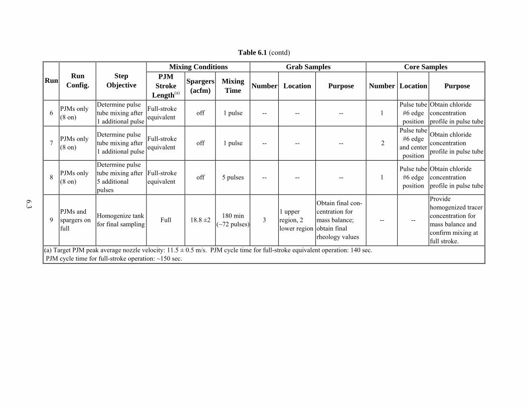
6.3

Table 6.1 (contd)


Run Run Config.

Step Objective

PJM Stroke

Length(a)

Spargers(acfm)

Mixing Time Number Location Purpose Number Location Purpose

6 PJMs only (8 on)





7 PJMs only (8 on)



Pulse tube #6 edge

and center position


8 PJMs only (8 on)


Full-stroke equivalent off 5 pulses -- -- -- 1




Homogenize tank for final sampling Full 18.8 ±2 180 min

(~72 pulses) 3 1 upper region, 2 lower region

Obtain final con-centration for mass balance; obtain final rheology values

-- --

Provide homogenized tracer concentration for mass balance and confirm mixing at full stroke.

(a) Target PJM peak average nozzle velocity: 11.5 ± 0.5 m/s. PJM cycle time for full-stroke equivalent operation: 140 sec. PJM cycle time for full-stroke operation: ~150 sec.

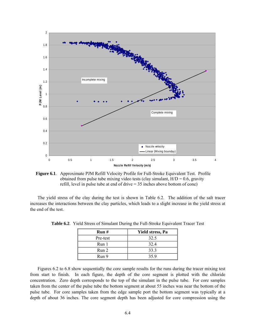
6.4

0

0.2

0.4

0.6

0.8

1

1.2

1.4

1.6

1.8

2

0 0.5 1 1.5 2 2.5 3 3.5 4


PJM

Lev

el (m

)

Nozzle velocityLinear (Mixing bounday)

Incomplete mixing

Complete mixing

Figure 6.1. Approximate PJM Refill Velocity Profile for Full-Stroke Equivalent Test. Profile

obtained from pulse tube mixing video tests (clay simulant, H/D = 0.6, gravity refill, level in pulse tube at end of drive = 35 inches above bottom of cone)

The yield stress of the clay during the test is shown in Table 6.2. The addition of the salt tracer increases the interactions between the clay particles, which leads to a slight increase in the yield stress at the end of the test.

Table 6.2. Yield Stress of Simulant During the Full-Stroke Equivalent Tracer Test

Run # Yield stress, Pa Pre-test 32.5 Run 1 32.4 Run 2 33.3 Run 9 35.9

Figures 6.2 to 6.8 show sequentially the core sample results for the runs during the tracer mixing test from start to finish. In each figure, the depth of the core segment is plotted with the chloride concentration. Zero depth corresponds to the top of the simulant in the pulse tube. For core samples taken from the center of the pulse tube the bottom segment at about 55 inches was near the bottom of the pulse tube. For core samples taken from the edge sample port the bottom segment was typically at a depth of about 36 inches. The core segment depth has been adjusted for core compression using the

6.5

information presented in Section 4.3.4. For comparison, the initial and final chloride concentrations are shown. These are based on analysis of grab samples taken before the tracer was added and after the vessel contents were homogenized at the end of the test. Core samples were taken from either the center or the edge sample ports, and the results from each port are identified in the plot legend by a C (center) or E (edge). Samples were analyzed in two batches approximately 1 month apart. The initial batch of 40 samples focused on the top 15 inches of the core sample. The second batch of 20 samples was analyzed to investigate the possibility of a “donut hole,” which is a region of unmixed simulant created when the refilling jet breaks through the surface and spreads over the top of the pulse tube contents. The results from the first batch of samples are shown as diamonds, while the results from the second batch of samples are shown as unfilled circles. Unfortunately, it appears that the samples from the second batch generally indicate concentrations that are lower by about 9%. The initial grab sample for the second batch gave a concentration of 160 ppm, while the initial sample from the first batch gave a concentration of 175 ppm. The other sample results appear low by a similar amount. The following causes were evaluated to explain the differences:

Bias in the analytical method/instrument: the stated accuracy of the ion chromatography anion method is ±10%, although results within a given batch are often much more accurate than ±10%. All quality control samples for both batches were within the acceptance criteria. The continuing calibration verification standards indicate that the results from both batches could be biased high. The relative bias between the two batches can account for about 4% of the difference between the two batches.

Absorption on the clay or precipitation of the tracer: testing conducted during the develop-ment of the chloride tracer test did not indicate appreciable absorption by the clay, although tests did not extend for more than a few days. It is plausible that interaction between the chloride ion and the clay matrix could account for the remaining difference between the two sample batches.

Evaporation: the sample bottles were well sealed and stored double bagged. In any case, evaporation would have increased the concentrations measured in the second batch.

While the cause of the difference in the analytical results of the two sample batches is not known with certainty, it is probably due to a combination of analytical bias and interaction of the chloride tracer with the sample matrix. Assuming the total bias between the two batches is 9%, the results for batch 2 were adjusted upward by 9% and are also plotted in Figures 6.2 through 6.8 as solid circles. Examination of Figure 6.2 (Run 2, initial baseline concentration in PJM #6 after the tracer addition) indicates that some tracer migrated into the bottom portion of the pulse tube while the tracer was being added and mixed in the simulant. The sample results from both batches support this observation. Even though the test pulse tube (#6) was in the vent mode and not operating, the variation in the simulant height outside the pulse tube during each PJM stroke probably caused some minor movement in PJM #6. Because the top portion of the pulse tube contents was not significantly affected, the test results were not compromised.

6.6

0

12

24

36

48

60

140

160

180

200

220

240

260

280

300

Cl-, ppm

Cor

e S

egm

ent D

epth

(inc

hes)

Initial - Batch 1

Initial - Batch 2

Homogenized - Batch 1

Run 2; PJM 6C - Batch 1


Run 2; PJM 6C - Batch 2Corrected

Figure 6.2. Core Sample Results for Run 2 (initial baseline concentration in PJM #6)a

Figure 6.3 shows the concentration profile after a single full-stroke equivalent cycle (Run 3) and indicates that there was significant mixing near the top of the simulant. The top core segments show a higher concentration than the lower segments. This indicates that there was a “donut hole” effect. This occurs because the refill jet punches up through the simulant and spreads out over the top of the pulse tube contents. This result is consistent with the visual observations obtained with the video camera, which showed the refill jet breaking through the surface near the side of the pulse tube opposite the pulse tube nozzle (see Figure 3.3). Figures 6.4 through 6.8 show the progressive mixing of the pulse tube contents as the number of pulses increases. In Figure 6.5 (3 cycles at full-stroke equivalent) it can be seen that the batch 1 and adjusted batch 2 results are approaching similar concentration values, indicating that the pulse tube contents are approaching a mixed state. Figures 6.6 (4 cycles at full-stroke equivalent) through 6.8 (10 cycles at full-stroke equivalent) also show that the batch 1 and adjusted batch 2 results have similar concentration values. Figure 6.9 shows concentrations at a depth of 6 and 30 inches as a function of pulse number. The concentrations were interpolated from the plots in Figures 6.2 through 6.8. The concentrations at 6 inches are based on the results from batch 1 samples, and the concentrations at 30 inches are based on unadjusted results from batch 2 samples. It can be seen that, after 3 cycles, there is little change in the concentrations at either depth. This indicates that mixing of the pulse tube contents was reasonably complete at this point. a The initial concentrations are based on grab samples taken prior to the addition of the tracer. The homogenized sample concentration is based on grab samples obtained at the end of the test after complete homogenization of the clay simulant.

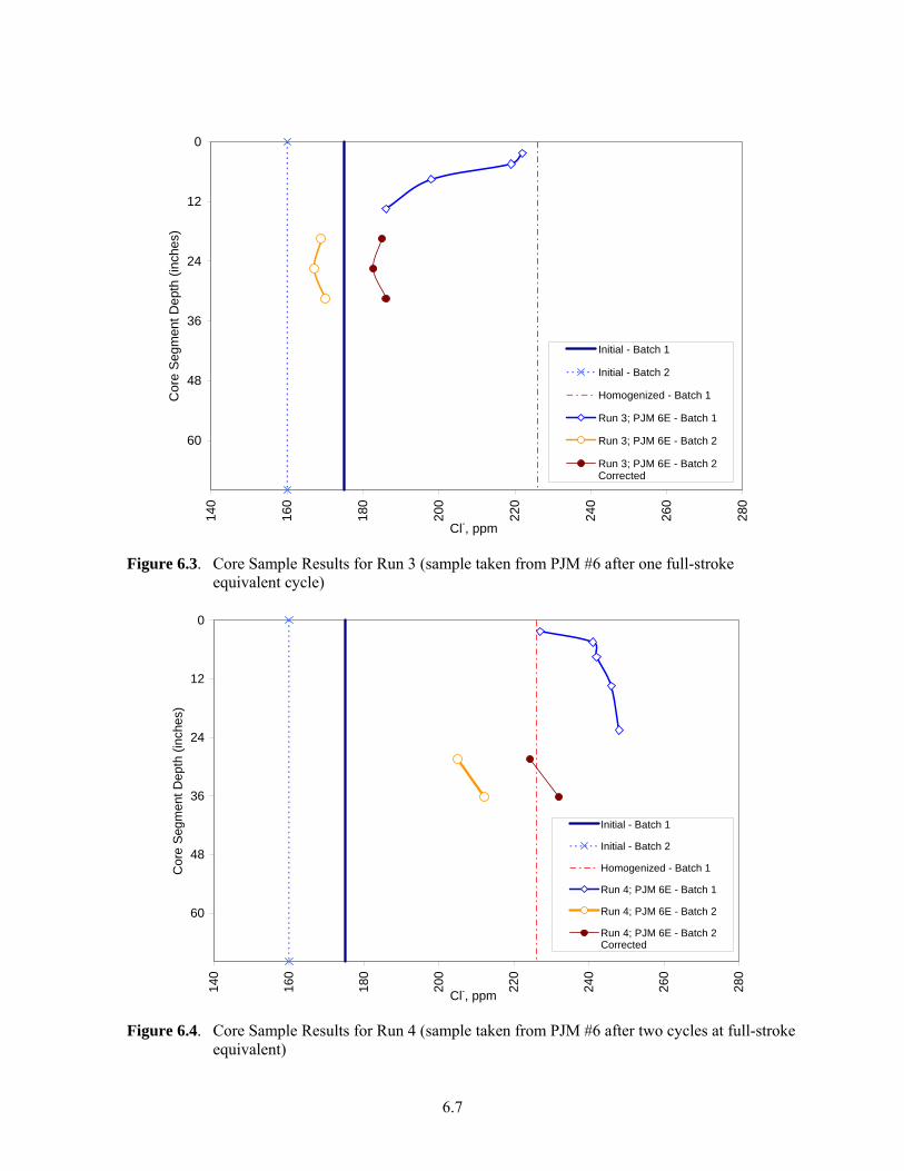
6.7

0

12

24

36

48

60

140

160

180

200

220

240

260

280

Cl-, ppm

Cor

e S

egm

ent D

epth

(inc

hes)

Initial - Batch 1

Initial - Batch 2


Run 3; PJM 6E - Batch 1


Run 3; PJM 6E - Batch 2Corrected

Figure 6.3. Core Sample Results for Run 3 (sample taken from PJM #6 after one full-stroke

equivalent cycle)

0

12

24

36

48

60

140

160

180

200

220

240

260

280

Cl-, ppm

Cor

e Se

gmen

t Dep

th (i

nche

s)

Initial - Batch 1

Initial - Batch 2





Figure 6.4. Core Sample Results for Run 4 (sample taken from PJM #6 after two cycles at full-stroke

equivalent)

6.8

0

12

24

36

48

60

140

160

180

200

220

240

260

280

Cl-, ppm

Cor

e Se

gmen

t Dep

th (i

nche

s)

Initial - Batch 1

Initial - Batch 2





Figure 6.5. Core Sample Results for Run 5 (sample taken from PJM #6 after three cycles at

full-stroke equivalent)

0

12

24

36

48

60

140

160

180

200

220

240

260

280

Cl-, ppm

Cor

e Se

gmen

t Dep

th (i

nche

s)

Initial - Batch 1

Initial - Batch 2





Figure 6.6. Core Sample Results for Run 6 (samples taken from PJM #6 after four cycles at


6.9

0

12

24

36

48

60

140

160

180

200

220

240

260

280

Cl-, ppm

Cor

e S

egm

ent D

epth

(inc

hes)

Initial - Batch 1

Initial - Batch 2






Run 7; PJM 6C - Batch 2 Corrected

Run 7; PJM 6E - Batch 2 Corrected

Figure 6.7. Core Sample Results for Run 7 (samples taken from PJM #6 after five cycles at


0

12

24

36

48

60

140

160

180

200

220

240

260

280

Cl-, ppm

Cor

e S

egm

ent D

epth

(inc

hes)

Initial - Batch 1

Initial - Batch 2





Figure 6.8. Core Sample Results for Run 8 (sample taken from PJM 6 after 10 cycles at full-stroke

equivalent)

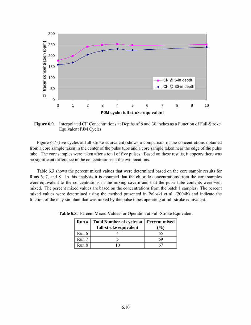
6.10

0

50

100

150

200

250

300

0 1 2 3 4 5 6 7 8 9 10

PJM cycle: full stroke equivalent

Cl- tr

acer

con

cent

ratio

n (p

pm)

Cl- @ 6-in depthCl- @ 30-in depth

Figure 6.9. Interpolated Cl- Concentrations at Depths of 6 and 30 inches as a Function of Full-Stroke Equivalent PJM Cycles

Figure 6.7 (five cycles at full-stroke equivalent) shows a comparison of the concentrations obtained from a core sample taken in the center of the pulse tube and a core sample taken near the edge of the pulse tube. The core samples were taken after a total of five pulses. Based on these results, it appears there was no significant difference in the concentrations at the two locations. Table 6.3 shows the percent mixed values that were determined based on the core sample results for Runs 6, 7, and 8. In this analysis it is assumed that the chloride concentrations from the core samples were equivalent to the concentrations in the mixing cavern and that the pulse tube contents were well mixed. The percent mixed values are based on the concentrations from the batch 1 samples. The percent mixed values were determined using the method presented in Poloski et al. (2004b) and indicate the fraction of the clay simulant that was mixed by the pulse tubes operating at full-stroke equivalent.

Table 6.3. Percent Mixed Values for Operation at Full-Stroke Equivalent

Run # Total Number of cycles at full-stroke equivalent

Percent mixed (%)

Run 6 4 65 Run 7 5 69 Run 8 10 67

7.1

7.0 Conclusions and Recommendations The results of the video camera mixing tests conducted in the HSLS test stand indicate that the height to which the non-Newtonian fluid with a yield stress in a refilling pulse tube can be mixed increases approximately linearly with the refill nozzle velocity. A comparison of the video camera results with the tracer results indicates that the conditions at which the surface agitation is observed is reasonably consistent with the extent of mixing found in the tracer experiment. A model based on turbulent jet theory was developed for mixing of the material in a pulse tube during refill. This model accounts for the decay of the jet with distance and the receding surface of the fluid in the pulse tube. Comparison of this model with results of the video camera mixing experiments shows reasonable agreement with the data. These test results obtained in the HSLS test stand indicate that a PJM mixing a non-Newtonian slurry with a yield stress of 30 Pa and employing the normal “full stroke” (80 to 85% of the pulse tube volume) will fully mix the pulse tube contents. The pulse tube mixing tracer test results indicate that the pulse tube contents were not completely mixed with the PJMs operating at “half stroke” (40% of the pulse tube volume). In the test operated using half strokes, a slug approximately 22.5 inches thick at the top of the simulant column was not mixed with a maximum nozzle refill velocity of ~2.6 m/s. The results further indicate that operation of these PJMs at ~86% of full stroke (73% of the PJM volume) would have been required to fully mix the slurry within the PJM. Alternatively, increasing the peak refill velocity to about 4.5 m/s would be required for half-stroke operation to provide complete mixing at the conditions tested. A peak refill velocity in excess of 5.1 m/s would be required for ideal half-stroke operation to provide complete mixing of the pulse tube contents. A pulse tube mixing tracer test conducted in the HSLS test stand with the PJMs operating at full-stroke equivalent indicated that the pulse tube contents are reasonably well mixed after 3 strokes. To apply these results to make an assessment of the full-scale (i.e. plant scale) mixing behavior in a pulse tube, additional information is needed, along with either additional testing at different scales or analysis using an appropriate CFD model. Full-scale refill functions will be needed for an estimate of the dimensionless refill velocity and acceleration. If the dimensionless acceleration and velocity at full scale is greater than or equal to the values at half-scale, then we expect the mixing results obtained at half scale to be conservative because the jet Reynolds number will be larger at full-scale; mixing is expected to improve as the jet Reynolds number increases. However, if the dimensionless acceleration of the full-scale refill function is smaller than at half scale, it is possible that the test results could be nonconservative. The location of the mixing line determined in the half-scale tests will also need to be estimated at full scale. This may be obtained by additional pulse tube mixing tests at different scales. Alternatively, it may be possible to estimate the location of the mixing line using an appropriate CFD model.

8.1

8.0 References Bamberger JA, PA Meyer, JR Bontha, CW Enderlin, DA Wilson, AP Poloski, JA Fort, ST Yokuda, HD Smith, F Nigl, M Friedrich, DE Kurath, GL Smith, JM Bates, and MA Gerber. 2005. Technical Basis for Testing Scaled Pulse Jet Mixing Systems for Non-Newtonian Slurries. PNWD-3551 (WTP-RPT-113 Rev. 0), Battelle – Pacific Northwest Division, Richland, Washington. Blomqvist S. June 1991. Quantitative Sampling of Soft-Bottom Sediments - Problems and Solutions. Marine Ecology-Progress Series, 72(3):295-304. Bontha JR, LK Jagoda, CW Stewart, CD Johnson, DE Kurath, KS Koschik, PA Meyer, DL Lessor, ST Arm, F Nigl, CE Guzman-Leong, RL Russell, MS Fountain, GL Smith, M Friedrich, W Yantasee, SA Hartley, and ST Yokuda. 2005. Technical Basis for Predicting Mixing and Flammable Gas Behavior in the Ultrafiltration Feed Process and High-Level Waste Lag Storage Vessels with non-Newtonian Slurries. PNWD-3676 (WTP-RPT-132 Rev 0), Battelle – Pacific Northwest Division, Richland, Washington. Johari H and Q Zhang. 1996. “Effects of Acceleration on Turbulent Jets.” Phys. Fluids, 8:2185. Morton RA and WA White. 1997. “Characteristics of and Corrections for Core Shortening in Unconsolidated Sediments.” Journal of Coastal Research, 13(3):761-769. Meyer PA, DE Kurath, and CW Stewart. 2005. Overview of the Pulse Jet Mixer Non-Newtonian Scaled Test Program. PNWD-3677 (WTP-RPT-127 Rev. 0), Battelle – Pacific Northwest Division, Richland, Washington. Poloski AP, PA Meyer, LK Jagoda, and PR Hrma. 2004a. Non-Newtonian Slurry Simulant Development and Selection for Pulsed Jet Mixer Testing. PNWD-3495 (WTP-RPT-111 Rev 0), Battelle – Pacific Northwest Division, Richland, Washington. Poloski AP, LA Snow, and ST Arm. 2004b. Chemical Tracer Techniques for Assessing Mixing Performance in non-Newtonian Slurries for WTP Pulsed Jet Mixer Systems. PNWD-3494 (WTP-RPT-121 Rev. 0), Battelle – Pacific Northwest Division, Richland, Washington.

Appendix

Comparison of Experimental Half and Full Strokes with Ideal Half and Full Strokes and Definition of

Full-Stroke Equivalent

A.1

Appendix

Comparison of Experimental Half and Full Strokes with Ideal Half and Full Strokes and Definition of Full-Stroke Equivalent Figures A.1 through A.4 show the simulant level and the stroke length for half- and full-stroke operation in relation to the tank and pulse tube dimensions. Figures A.1 and A.3 show the actual half- and full-stroke dimensions obtained in the perimeter pulse tubes in the half-scale lag storage (HSLS) test stand; Figures A.2 and A.4 show ideal half and full strokes in the perimeter pulse tubes in the HSLS test stand. The maximum simulant refill level for both half- and full-stroke operation was about 18 inches below the top of the pulse jet mixer (PJM). In normal plant operation, the pulse tubes are completely filled prior to the start of the next drive. The pulse tubes were not completely filled because the vacuum applied during refill was reduced to provide a minimum refill velocity for testing. As shown in Figure A.1, the drive length for half-stroke operation was 35 inches and ended about 8 inches below the location of an ideal half-stroke drive. As discussed in Section 5.2 of the main report, the volume of simulant expelled from the pulse tube was 41% of a full stroke, which is less than the target of 50%. Although this is an important consideration for analysis of cavern size, it is inconsequential for the purpose of refill mixing analysis. The effect of the drive stroke ending 8 inches low was accounted for in the mixing analysis in Section 5.4 of the report. As shown in Figure A.3, the drive length for full-stroke operation was 71 inches and ended about 1 inch below the location of an ideal full-stroke drive. As discussed in Section 5.2 of the main report, the volume of simulant expelled from the pulse tube was 83% of a full stroke, which is less than the target of 100%. Although this is an important consideration for analysis of cavern size, it is inconsequential for the purpose of refill mixing analysis. The effect of the drive stroke ending 1 inch below the location for an ideal full-stroke drive is not considered significant because the level was well below the level where full mixing of the pulse tube contents occurred. In addition, the experimental error associated with the level measurements is at least 1 inch. Figure A.5 shows the simulant level and the stroke dimensions for the full-stroke equivalent operation in relation to the tank and pulse tube dimensions. The stroke started with the simulant level at the level of the simulant in the tank. This stroke length corresponds to a stroke that would expel 80% of the pulse tube contents if the pulse tube had been completely filled during the refill portion of the PJM cycle.

A.2

Figure A.1. Actual Half Stroke in Tracer Mixing Experiment for Perimeter PJM (all dimensions are in inches)

6

90 39

19

50

44

78

39

91

87 or H/D = 0.57

6

12

62

70 97

Maximum refill level

End of drive for half stroke

18

8

35

Reference (0-in)

50

44

90

12

6

A.3

Figure A.2. Ideal Half Stroke in the HSLS Test Stand for Perimeter PJM (all dimensions are in inches)

6

90 39

19

50

44

78

39

91

87 or H/D = 0.57

6

12

70 115


End of drive for half stroke

45

Reference (0-in)

50

44

90

6

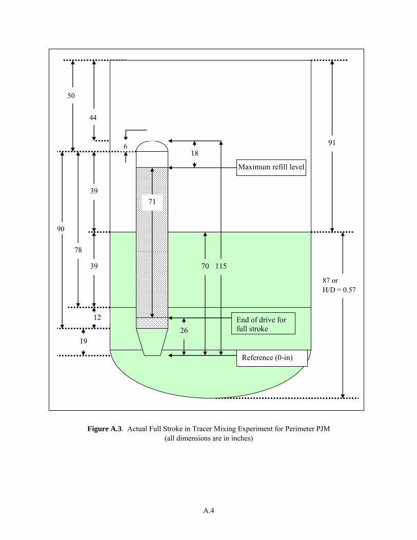
A.4

Figure A.3. Actual Full Stroke in Tracer Mixing Experiment for Perimeter PJM (all dimensions are in inches)

90

6

39

19

50

44

78

39

91 6

12

26

70 115


End of drive for full stroke

71

18

Reference (0-in)

87 or H/D = 0.57

50

44

90

6

A.5

Figure A.4. Ideal Full Stroke in HSLS Test Stand for Perimeter PJM (all dimensions are in inches)

90

87 or H/D = 0 57

6

39

19

50

44

78

39

91 6

12

27

115


End of drive for full stroke

88

Reference (0-in)

87 or H/D = 0.57

50

44

90

6

A.6

6

35.7

19

50

44

76.7

41

91 6

13.3

32.3

115


End of drive for full stroke equivalent

35.7

Reference (0-in) 51.3

19

90

126.7

87 or H/D = 0.57

Figure A.5. Full Stroke in Equivalent in HSLS Test Stand for Perimeter PJM (all dimensions are in inches)

PNWD-3827 WTP-RPT-155 Rev. 0

Distr. 1

Distribution

No. of Copies OFFSITE

No. of Copies ONSITE

1 Savannah River National Laboratory Richard Edwards Savannah River National Laboratory Westinghouse SA Aiken, SC 29808-0001

10 Battelle – Pacific Northwest Division J. R. Bontha K6-24 M. D. Bleich K6-85 W. C. Buchmiller K6-24 W. H. Combs K7-15 J. A. Fort K7-15 P. A. Meyer K7-15 D. E. Kurath P7-28 A. P. Poloski P7-28 I. D. Welch K6-85 Project File (1) P7-28

8 Bechtel National, Inc.

S. M. Barnes H4-02 C. E. Corriveau H4-02 P. A. Fisher (2) H4-02 E. D. Johnson H4-02 D. E. Larson H4-02 P. G. Schmitz H4-02 K. L. Herman H4-02

assessment of pulse tube mixing for vessels … · rheological bound to assess pulse tube mixing...

Documents