This is an electronic reprint of the original article.This reprint may differ from the original in pagination and typographic detail.

Powered by TCPDF (www.tcpdf.org)

This material is protected by copyright and other intellectual property rights, and duplication or sale of all or part of any of the repository collections is not permitted, except that material may be duplicated by you for your research use or educational purposes in electronic or print form. You must obtain permission for any other use. Electronic or print copies may not be offered, whether for sale or otherwise to anyone who is not an authorised user.

Kortela, Jukka; Jämsä-Jounela, Sirkka-LiisaModeling and model predictive control of the BioPower combined heat and power (CHP) plant

Published in:International Journal of Electrical Power and Energy Systems

DOI:10.1016/j.ijepes.2014.10.043

Published: 01/01/2015

Document VersionEarly version, also known as pre-print

Please cite the original version:Kortela, J., & Jämsä-Jounela, S-L. (2015). Modeling and model predictive control of the BioPower combinedheat and power (CHP) plant. International Journal of Electrical Power and Energy Systems, 65(February 2015),453-462. https://doi.org/10.1016/j.ijepes.2014.10.043

Modeling and Model Predictive Control of the BioPower combined heat and power(CHP) plant

J. Kortelaa,1,∗, S-L. Jamsa-Jounelaa,1

aAalto University School of Chemical Technology, P.O. Box 16100, FI-00076 Aalto

Abstract

This paper presents a model predictive control (MPC) strategy for BioGrate boiler, compensating the main disturbancescaused by variations in fuel quality such as the moisture content of fuel, and variations in fuel flow. The MPC utilizesmodels, the fuel moisture soft-sensor to estimate water evaporation, and the fuel flow calculations to estimate the thermaldecomposition of dry fuel, to handle these variations, the inherent large time constants, and long time delays of the boiler.The MPC strategy is compared with the method currently used in the BioPower 5 CHP plant. Finally, the results arepresented, analyzed and discussed.

Keywords: combustion, biomass, fuel quality, MPC, moisture, advanced control

1. Introduction

The utilization of renewable energy sources is increas-ing due to demand to replace fossil energy sources withmore ecological ones. The biomass is one of these renew-able energy sources[1],[2]. BioGrate burns this fuel witha moisture content as high as 65% [3]. However, a vary-ing moisture content and varying fuel flow of the biomassresults in uncertainty about its energy content and com-plicates operation of BioGrate process.

Kortela and Lautala [4] developed a method in order toestimate how much fuel is burning at the time momentand combustion power based on the flue gas oxygen andthe air measurements, and the fuel composition. It wasreported that the amplitude and the settling time of theresponse of the boiler power decreased to about one-third-of the original.

Havlena and Findejs [5] employed model-based predic-tive control strategy to enable dynamical coordination be-tween fuel and air flows. This enabled the boiler to perma-nently operate with the optimum excess air, and resultedin reduced NOx production. Prasad et al. [6] tested theapplication of a multivariable long-range predictive control(LRPC) with global linear models and local model net-works in the simulation of a 200 MW oil-fired drum-boilerthermal plant. They reported extremely small variationsof±0.5 bar, ±1.0◦C, and±1.5◦C for steam pressure, steamtemperature, and reheat steam temperature, respectively.

∗Corresponding author. Tel.:+358 9 4702 2647; fax: +358 9 47023854.

Email addresses: jukka.kortela@aalto.fi (J. Kortela),sirkka-liisa.jamsa-jounela@aalto.fi (S-L. Jamsa-Jounela)

1E-mail addresses: jukka.kortela@aalto.fi (J. Kortela), sirkka-liisa.jamsa-jounela@aalto.fi (S-L. Jamsa-Jounela)

Swarnakar et al. [7] presented a scheme for robust sta-bilization of a boiler, based on linear matrix inequalities(LMIs). The simulation results showed that the proposedcontrol is effective against sudden load changes. However,BioGrate process needs a special consideration in its con-trol strategy development due to its long time delay of minseconds and moisture variations in fuel feed.

Bauer et al. [8] derived a simple model for the gratecombustion of biomass based on two mass balances fordry fuel and water. The model was verified by experi-ments at a pilot scale furnace with a horizontally movinggrate. The test results showed that the overall effect ofthe primary air flow rate on the thermal decomposition ofdry fuel is multiplicative. This is also shown in the resultsof Yang et al. [9] when the air factor is not much largerthan stoichiometric air, staying in a typical optimal levelfrom around 1.2 to 1.7. Higher air flows begin to cool thebed, decreasing the propagation rates [10]. In addition,the test results of Bauer et al. [8] showed that the waterevaporation rate is mainly independent of the primary air

amsa-Jounela [11] developed a fuel moisture soft sensor that isbased on a dynamic model that makes use of combustionpower estimates and that makes use of the model of thesecondary superheater.

This paper presents a model predictive control (MPC)strategy for a BioGrate boiler. The paper is organized asfollows: Section 2 presents The BioPower 5 CHP plantprocess and its control strategy. Section 3 presents theMPC strategy, and dynamic models, and fuel-moisturesoft-sensors of a boiler. The identifications of the mod-els of BioPower 5 CHP plant are presented in Section 4.The simulation results of the MPC strategy are presentedin Section 5, followed by the conclusions in Section 6.

Preprint submitted to Elsevier May 15, 2015

2. Description of the process and its control strat-egy

In the BioPower 5 CHP plant, the heat used for steamgeneration is obtained by burning solid biomass fuel: bark,sawdust and pellets, which are fed to the steam boilertogether with combustion air. As a result, combustionheat and flue gases are generated. The heat is then usedin the steam-water circulation process. The fuel is fedonto the center of a grate from below by a stoker screw.The grate is divided into concentric rings with alternaterotating rings and the rings between remaining stationary.Alternate rotating rings are pushed hydraulically clockwiseor counterclockwise respectively. This design distributesthe fuel evenly over the entire grate with the burning fuelforming an even layer of the required thickness [3].

The water content of the wet fuel in the centre of thegrate evaporates rapidly due to the heat of the surroundingburning fuel and thermal radiation from the brick walls.The gasification and visible combustion of the gases andsolid carbon take place as the fuel moves to the peripheryof the circular grate. Finally, at the edge of the grate, ashfalls into a water-filled ash basin underneath the grate [3].

The primary air for combustion, and the recirculationflue gas, are fed from underneath the grate and penetratethe fuel through slots in the concentric rings. Secondaryair is fed above the grate directly into the flame. Air distri-bution is controlled by dampers and speed-controlled fans[3].

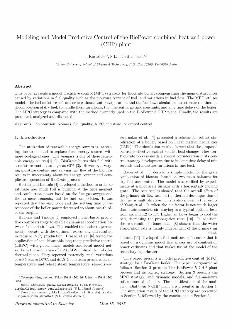
Fig. 2 shows the boiler part of the BioPower 5 CHPplant. The essential components of the water-steam cir-cuit are an economizer, a drum, an evaporator and super-heaters. Feed water is pumped from a feed water tank tothe boiler. First the water is led to the economizer (4)that is heated by flue gases. The temperature of flue gasesis decreased by the economizer, and the efficiency of theboiler is improved.

Figure 1: BioGrate including the stoker screw and a water-filled ashbasin underneath the grate

From the economizer, heated feed water is led to thedrum (5) and along downcomers into the bottom of the

evaporator (6) tubes that surround the boiler. From theevaporator tubes the heated water and steam return backto the steam drum, where steam and water are separated.Steam rises to the top of the steam drum and flows tothe superheaters (7). Steam heats up further so that itsuperheats. The superheated high-pressure steam (8) isled to a steam turbine, where electricity is generated.

2.1. Current control strategy of the BioPower plant

The main objective of the BioPower plant is to producea desired amount of energy by keeping the drum pressureconstant. The necessary boiler power is produced by ma-nipulating primary air, secondary air, and stoker speed asillustrated in Fig. 3.

The fuel feed is controlled by manipulating the motorspeed of the stoker screw to track the primary air flowmeasurement. The necessary amount of primary air andsecondary air for diverse power levels are specified by aircurves. The set point of the secondary air controller isadjusted by the flue gas oxygen controller to provide excessair for combustion and enable the complete combustion offuel.

3. Model predictive control for the BioPower 5CHP plant

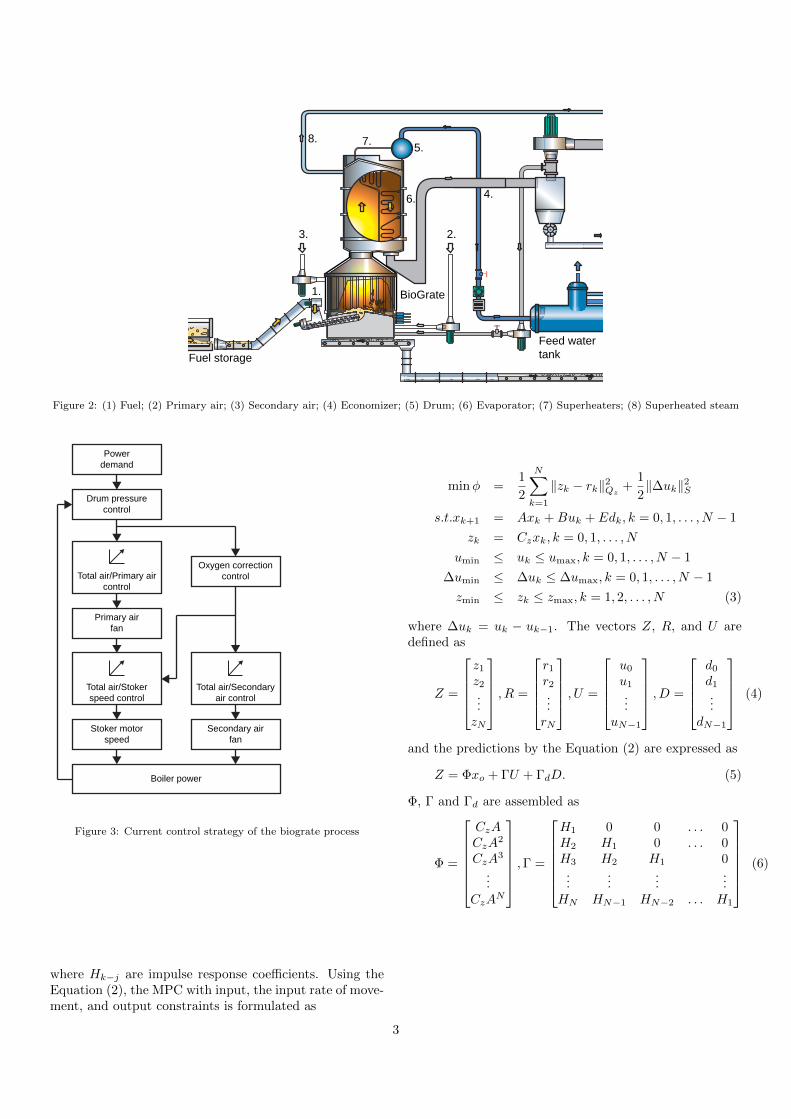
The improvised MPC strategy over the current controlstrategy is illustrated in Fig. 4. The proposed strategy uti-lizes fuel and moisture soft-sensors to estimate the burnedfuel and the water evaporation respectively. Subsequently,the combustion power is estimated based on these fuel-moisture soft sensors. As a result, the required amount ofcombustion power from the boiler can be produced, whichis done by manipulating the primary air and the stokerspeed. In addition, this combustion power can be accu-rately predicted.

3.1. MPC for BioGrate boiler

The primary air and the stoker speed are the input vari-ables (u); the fuel moisture content in the fuel feed andthe power demand are the measured disturbances (d); andthe combustion power and the drum pressure are the con-trolled variables (z), as illustrated in Fig. 5. The developedMPC utilizes the linear state space system as follows [12]:

xk+1 = Axk +Buk + Edk

zk = Czxk (1)

3.2. Regulator

The process is described by linear time invariant (LTI)state space model

zk = CzAkx0 +

k−1∑j=0

Hk−juj (2)

2

Feed watertankFuel storage

BioGrate

3. 2.

1.

5.

6.

8. 7.

4.

Figure 2: (1) Fuel; (2) Primary air; (3) Secondary air; (4) Economizer; (5) Drum; (6) Evaporator; (7) Superheaters; (8) Superheated steam

Powerdemand

Drum pressurecontrol

Total air/Primary aircontrol

Primary airfan

Total air/Stokerspeed control

Stoker motorspeed

Oxygen correctioncontrol

Total air/Secondaryair control

Secondary airfan

Boiler power

Figure 3: Current control strategy of the biograte process

where Hk−j are impulse response coefficients. Using theEquation (2), the MPC with input, the input rate of move-ment, and output constraints is formulated as

minφ =1

2

N∑k=1

‖zk − rk‖2Qz+

1

2‖∆uk‖2S

s.t.xk+1 = Axk +Buk + Edk, k = 0, 1, . . . , N − 1

zk = Czxk, k = 0, 1, . . . , N

umin ≤ uk ≤ umax, k = 0, 1, . . . , N − 1

∆umin ≤ ∆uk ≤ ∆umax, k = 0, 1, . . . , N − 1

zmin ≤ zk ≤ zmax, k = 1, 2, . . . , N (3)

where ∆uk = uk − uk−1. The vectors Z, R, and U aredefined as

Z =

z1z2...zN

, R =

r1r2...rN

, U =

u0u1...

uN−1

, D =

d0d1...

dN−1

(4)

and the predictions by the Equation (2) are expressed as

Z = Φxo + ΓU + ΓdD. (5)

Φ, Γ and Γd are assembled as

Φ =

CzACzA

2

CzA3

...CzA

N

,Γ =

H1 0 0 . . . 0H2 H1 0 . . . 0H3 H2 H1 0...

......

...HN HN−1 HN−2 . . . H1

(6)

3

Powerdemand

Drum pressurecontrol

Combustion powercontrol

Total air/Primary aircontrol

Primary airfan

Total air/Stokerspeed control

Stoker motorspeed

thermaldecomposition of fuel

Moistureevaporation

Oxygen correctioncontrol

Total air/Secondaryair control

Secondary airfan

Boiler power

Flue gasoxygen content

Combustion powerestimation

Figure 4: Model predictive control (MPC) strategy of BioGrate boiler

u1Primary air SP

u2Stoker speed SP Thermaldecomposition

of dry fuel

Waterevaporation

d1Moisture in fuel

-

Combustion powerestimation

-

Drumpressure

z2Drumpressure

z1Combustionpower

d2Power demand

Figure 5: Configuration of the boiler model of MPC strategy for BioPower 5 CHP plant

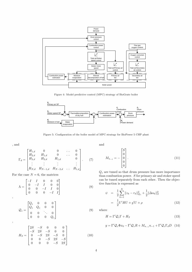
, and

Γd =

H1,d 0 0 . . . 0H2,d H1,d 0 . . . 0H3,d H2,d H1,d 0

......

......

HN,d HN−1,d HN−2,d . . . H1,d

. (7)

For the case N = 6, the matrices

Λ =

−I I 0 0 00 −I I 0 00 0 −I I 00 0 0 −I I

(8)

,

Qz =

Qz 0 0 0Qz Qz 0 0

0 0. . . 0

0 0 0 Qz

(9)

,

HS =

2S −S 0 0 0−S 2S −S 0 00 −S 2S −S 00 0 −S 2S −S0 0 0 −S 2S

(10)

and

Mu−1= −

S0000

. (11)

Qz are tuned so that drum pressure has more importancethan combustion power. S for primary air and stoker speedcan be tuned separately from each other. Then the objec-tive function is expressed as

ψ =1

2

N∑k=1

‖zk − rk‖2Qz+

1

2‖∆uk‖2S

=1

2U ′HU + g′U + ρ (12)

where

H = Γ′QzΓ +HS (13)

g = Γ′QzΦx0 − Γ′QzR+Mu−1u−1 + Γ′QzΓdD (14)

4

The MPC regulator problem Equation (3) can be solvedby the solution of the following convex quadratic program

minU

ψ =1

2U ′HU + g′U

Umin ≤ U ≤ Umax

∆Umin ≤ ΛU ≤ ∆Umax

Zmin ≤ ΓU ≤ Zmax (15)

where

Zmin = Zmin − Φxo − ΓdD (16)

Zmax = Zmax − Φxo − ΓdD (17)

In order to achieve offset-free performance, the state ofthe system is augmented with an integrating disturbancevector [13]. The designed system uses an input disturbancemodel where Bd = B, Ad is the unit matrix and Cη is thezero matrix.[

xk+1

ηk+1

]=

[A Bd0 Ad

] [xkηk

]+

[B0

]uk +

[E0

]dk +

[wkξk

](18)

yk =[C Cη

] [xkηk

]+ vk (19)

where xk are the states and ηk the integrating disturbancestates. The state and the additional integrating distur-bance are estimated from the plant measurement by usinga Kalman filter designed for the augmented system. Thevectors wk and vk are white-noise disturbances with zero-mean for the augmented state equation and the outputequation, respectively. Thus, the state and the distur-bance of the system are estimated as follows:[

xk|kηk|k

]=

[xk|k−1ηk|k−1

]+

[LxLη

](yk − Cxk|k−1 − Cη ηk|k−1) (20)

where xk are the state estimations, and the ηk disturbanceestimations. The prediction of the state of the augmentedsystem is obtained by[

xk+1|kηk+1|k

]=

[A Bd0 Ad

] [xk|kηk|k

]+

[B0

]uk +

[E0

]dk (21)

Additional disturbances, ηk, are not controllable by the in-puts u. However, since they are observable, their estimatesare used to remove their influence from the controlled vari-ables. The disturbance model is defined by choosing thematrices Bd and Cη. Since the additional disturbancemodes introduced by disturbance are unstable, it is neces-sary to check the detectability of the augmented system.The augmented system in Equation (18) is detectable ifand only if the nonaugmented system in Equation (1) isdetectable, and the following condition holds:

rank

[I −A −BdC Cη

]= n+ nη (22)

In addition if the system is augmented with a number ofintegrating disturbances nη equal to the number of themeasurements p (nη = p) and if the closed-loop system isstable and constraints are not active at steady state, thereis zero offset in controlled variables

3.3. Modeling of BioGrate boiler for MPC

An unknown flue flow and the water evaporation rate re-sults in uncertainty in the combustion power. Therefore,the models of the boiler include, model for water evapora-tion, the model for themal decomposition of fuel, and thedrum model.

3.3.1. The model of water evaporation

The model of water evaporation is [8]

dmw(t)

dt= −cwevmw(t)αwev(t)

+dmw,in(t− Td(t))

dt[kg/s] (23)

where cwev is the correction coefficient, αwev is the coeffi-cient for a dependence on the position of the moving grate,and mw,in the moisture in the fuel feed (kg/s).

Td(t) = cdmw(t)

αds,inmds,in(t)[s] (24)

where cd is the delay coefficient, αds,in is the stoker speedcorrection coefficient (kg/s/%), and mds,in(t) is the stokerspeed (%).

mw,in(t) =

∫ t

0

mw,in(τ) dτ [kg] (25)

3.3.2. The model of thermal decomposition of dry fuel

The model of thermal decomposition of dry fuel is [8]

dmds(t)

dt= −cthdmds(t)αthd(t)[mpa(t) + mpa,0]

+dαds,inmds,in(t− Td(t))

dt[kg/s] (26)

where cthd is the thermal decomposition rate coefficient,αthd(t) is the coefficient for a dependence on the positionof the moving grate, mpa(t) is the primary air flow rate bias(kg/s), and mpa,0(t) the primary air flow rate in (kg/s).

mds,in(t) =

∫ t

0

mds,in(τ) dτ [kg] (27)

For the linear state space model of Equation (1), the Equa-tion (26) is linearized as

dmds(t)

dt= −cdsmds(t)− cpampa(t)

+dαds,inmds,in(t− Td(t))

dt[kg/s] (28)

where cds is the fuel bed height coefficient, and cpa theprimary air flow coefficient.

5

3.3.3. Drum model

The drum level is kept at a constant level by its con-troller, and therefore the variations in the steam volumeare small. Thus, the drum model is [14]

dp

dt=

1

e(Q− mf (hw − hf )

−ms(hs − hw)) (29)

e ≈ %wVw∂hw∂p

+mtCp∂Ts∂p

(30)

where Q is the combustion power (MJ/s), mf is the feedwater flow (kg/s), hw is the specific enthalpy of the wa-ter (MJ/kg), hf is the specific enthalpy of the feed water(MJ/kg), ms is the steam flow rate (kg/s), hs is the specificenthalpy of the steam (MJ/kg), %w is the specific densityof the water (kg/m3), Vw is the volume of the water (m3),mt is the total mass of the metal tubes and the drum (kg),and Cp is specific heat of the metal (MJ/kgK).

3.3.4. Fuel flow soft-sensor

The elemental composition, and moisture content of afuel have a strong effect on its heat value. If fuel containsmoisture, this evaporates when the fuel is burned, but thisevaporation requires energy, which is absorbed from theheat of the fuels combustion and decreases its heat value.The effective heat value of a dry fuel is

qwf = 0.348 · wC + 0.938 · wH + 0.105 · wS+0.063 · wN − 0.108 · wO[MJ/kg] (31)

where wC is the carbon in the fuel (%), wH is the hydrogenin the fuel (%), wS is the sulfur in the fuel (%), wN is thenitrogen in the fuel (%), and wO the oxygen in the fuel(%). The effective heat value of a wet fuel is obtainedusing the equation

qf = qwf · (1− w/100)− 0.0244 · w[MJ/kg] (32)

where w is the moisture content of the wet fuel (%). Inorder to use Equation (31) and Equation (32), the compo-sition of the fuel has to be known.

Oxygen consumption signals how much fuel is burningat the time moment. This information can be used tocalculate the combustion power of the burned fuel. Theamount of oxygen needed to burn one kilogram of the fuelis

NgO2

= nC + 0.5 · nH2+ nS − nO2

[mol/kg] (33)

where nC is the carbon (mol/kg), nH2 is the hydrogen(mol/kg), nS is the sulfur (mol/kg), and nO2

the oxygen(mol/kg). Combustion air includes 3.76 times more nitro-gen than oxygen. The flue gas flow to burn one kilogramof fuel is thus

Nfg = nC + nH2+ nS + 3.76 ·Ng

O2+ nN2

+ nH2O[mol/kg](34)

where nH2O is the water (mol/kg). Similarly, the flue gaslosses per kilogram of fuel are determined by:

qgfg = (nCCCO2+ nSCSO2

+ (nH2O + nH2)CH2O

+(3.76 ·NgO2

+ nN2)CN + (FAir/(22.41 · 10−3 · mthd(w))

−4.76 ·NgO2

)CAir) · (Tfo − T0)[J/kg] (35)

where Ci is the specific heat capacity of the component i(J/molT), FAir is total air flow (m3/s), mthd is the the-mal decomposition of fuel (kg/s), Tfo is the flue gas tem-perature after the economizer (◦C), and T0 the referencetemperature (◦C). The thermal decomposition of fuel iscalculated as follows [11], that is estimated amount fuelburning at the time moment:

mthd(w) =(0.21− XO2

100 )nAir

NgO2

+XO2

100 (Nfg − 4.76 ·NgO2

)[kg/s] (36)

where XO2(t+ τ) is the flue gas oxygen content (%), andnAir the sum of the primary and secondary air flows (to-tal air) (mol/s). The net combustion power for the giventhermal decomposition of fuel is

Q = mthd(w)(qf − qgfg − qcr)[MJ] (37)

where qgfg is the flue gas loss (MJ/kg), and qcr the convec-tion and radiation losses (MJ/kg), which are typically 1.5% of the effective heat value qf . Flue gas flow for fuel flowin Equation 36 is given by:

mfg = FAir + mthd(w)(Nfg − 4.76 ·NgO2

) · 22.41 · 10−3[m3/s] (38)

Where as the temperature before the secondary super-heater is calculated using:

Tfg = (qf + 0.21(FAir/(22.41 · 10−3 · mthd(w))CO2

+0.79(FAir/(22.41 · 10−3 · mthd(w))CN2)/

(nCCCO2+ nSCSO2

+ (nH2O + nH2)CH2O

+(3.76 ·NgO2

+ nN2)CN2

+ 0.21 ·NExAirCO2

+0.79 ·NExAirCN2)[◦C] (39)

where the NEAir excess air (mol/kg).

3.3.5. Fuel moisture soft-sensor

The fuel moisture soft-sensor assumes that a change inthe water evaporation rate affects the enthalpy of the sec-ondary superheater; The effective value of the fuel qgfchanges linearly when the water evaporation rate changes[15]. The water evaporation rate w is obtained by mini-mizing

min J(w) =N∑i=0

|h2 − h2| (40)

where N is the prediction horizon, h2 is the specific en-thalpy after the secondary superheater (MJ/kg), and h2is the estimated specific enthalpy after the secondary su-

6

perheater (MJ/kg). The prediction model for the specificenthalpy after the secondary superheater is

dh2dt

=1

%V(Qt + m1h1 − m2h2)[MJ/(s · kg)] (41)

where % is the specific density of the steam (kg/m3), Vis the volume of the steam of the secondary superheater(m3), m1 is the steam flow before the secondary super-heater (kg/s), h1 is the specific enthalpy before the sec-ondary superheater (MJ/kg), and m2 is the steam flowafter the secondary superheater (kg/s). The heat trans-fer from the flue gas to the metal tubes of the secondarysuperheater in the presence of mixed convection and radi-ation heat transfer is

Qw = αwm0.65fg ((Tfg − αfo ∗ Tfo)− Tw)

+kw((Tfg − αfo ∗ Tfo)4 − T 4w)[MJ/s] (42)

where αw is the convection heat transfer coefficient, αfo isthe correction coefficient, Tfo is the flue gas temperatureafter the economizer (◦C), Tw is the temperature of themetal tubes of the secondary superheater (◦C), and kw isthe radiation heat transfer coefficient. The temperature ofthe tube walls of the secondary superheater is

dTwdt

=1

mtCp(Qw −Qt)[K/s] (43)

where mt is the mass of the metal tubes of the secondarysuperheater (kg), and Cp is the specific heat capacity ofthe metal (MJ/kgK). The heat transfer from the metaltubes of the secondary superheater to the steam in thepresence of convection heat transfer is

Qt = αcm0.82 (Tw − T )[MJ/s] (44)

where αc is the convection heat transfer coefficient.

T = (T1 + T2)/2[◦C] (45)

where T1 is the steam temperature before the secondarysuperheater (◦C) and T2 the steam temperature after thesecondary superheater (◦C).

4. Test results of system identification of modelparameters of BioGrate boiler

The identification of models of the water evaporation,the thermal decomposition of dry fuel, and the drumpressure was conducted using the measurements of theBioPower 5 CHP plant. For the fuel feed, the sampleswere taken every 5 min from fuel dropping from the fuelsilo just before the stoker screw and analyzed manually.The Servomex 2500 FT-IR analyzer was used to measurethe water evaporation. The flue gas was extracted fromthe flue gas duct and led into the analyzer. The sampleswere taken every second. The compression factors for themeasurements of the BioPower 5 CHP plant were detectedas follows:

Table 1: The compression factors of the measurementsMeasurement Compression factor (s)Pressure 182Steam temperature 395Steam flow 10Feed water pressure 320Feed water temperature 5082Feed water flow 6Primary air flow 4Secondary air flow 6Flue gas oxygen content 75Flue gas moisture content 25Stoker speed 367

∆(∆)i =yi+1 − 2yi + yi−1

h2(46)

where y is a reconstructed signal and h is the samplinginterval. The index i ranges from 2 to N − 1, where N isthe number of samples. If the reconstructed data is differ-enced twice, there will be n = N −m second differenceswhose values are zero. Therefore, the compression factoris determined from

CF est =N

m(47)

where m = N − n. The compression factor of the mea-surements are presented in Table 1.

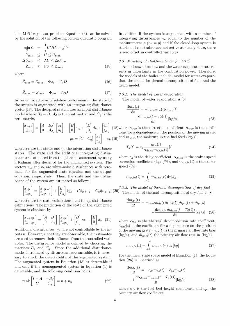
Fig. 6 shows the estimated and measured water evapora-tion based on the measured data. The model performanceis illustrated in Fig. 7. Due to the longer sampling timeof 5 minutes of the fuel feed, the estimated values and themeasurements are not exactly the same.

0 1000 2000 3000 4000 500030

40

50

60

Wat

er e

vapo

ratio

n (%

)

0 1000 2000 3000 4000 500020

30

40

50

60

Fue

l moi

stur

e (%

)

Time (s)

Figure 6: The measured (dashed line) and estimated (solid line)water evaporation, and input parameter, the moisture content offuel feed in the identification. The delay between input and outputvariables is 20 minutes

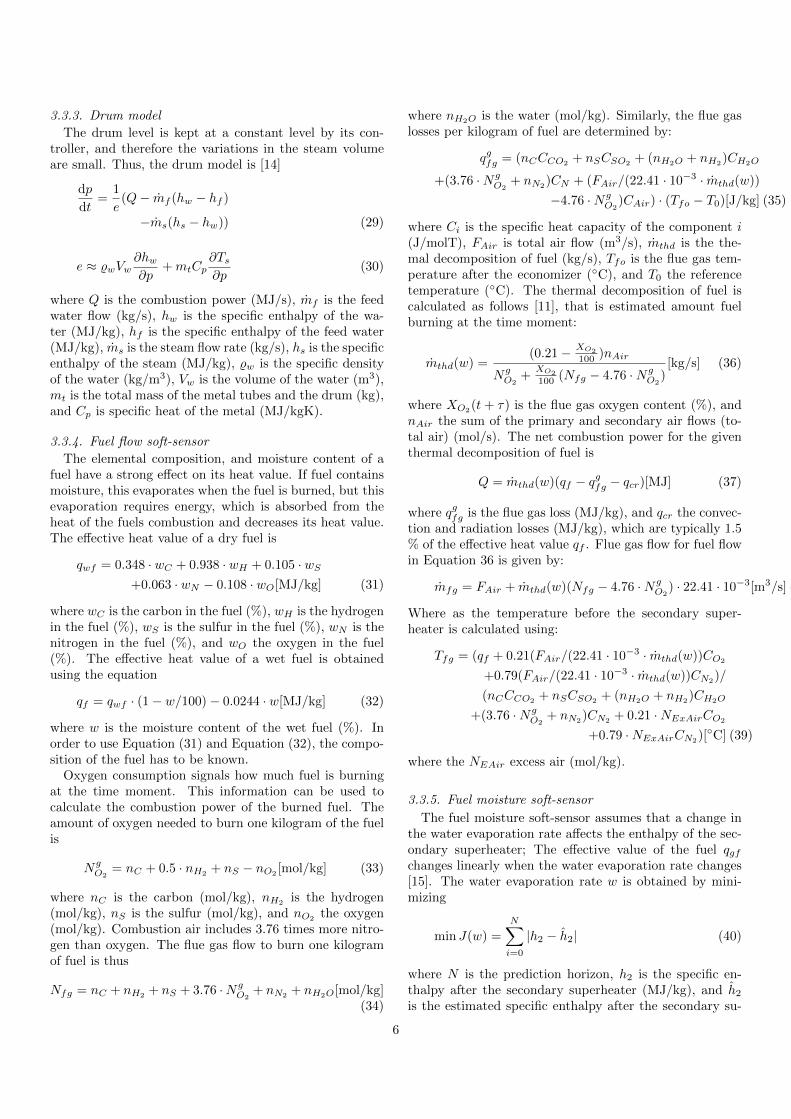
Fig. 8 shows the estimated and measured thermal de-composition of fuel. The validation of the identified modelwas performed on another measurement series. The modelperformance is presented in Fig. 9. The good performance

7

0 500 1000 1500 200020

30

40

50

60

Wat

er e

vapo

ratio

n (%

)

0 500 1000 1500 200020

40

60

80

Fue

l moi

stur

e (%

)

Time (s)

Figure 7: The measured (dashed line) and estimated (solid line)water evaporation, and the input parameter, the moisture contentof fuel feed in the validation. The delay between input and outputvariables is 20 minutes.

of the model was due to the constant fuel bed height ofgrate that affects the thermal decomposition of the fuel.

0 1000 2000 3000 4000 5000 6000 7000 8000

2

3

4

The

rmal

dec

ompo

sitio

nof

bio

mas

s fu

el (

kg/s

)

0 1000 2000 3000 4000 5000 6000 7000 80002

4

6

Prim

ary

air

(m3 /s

)

0 1000 2000 3000 4000 5000 6000 7000 800020

40

60

Sto

ker

spee

d (%

)

Figure 8: The measured (dashed line) and estimated (solid line) ther-mal decomposition of biomass fuel, and the model input parameters,primary air and stoker speed in the identification.

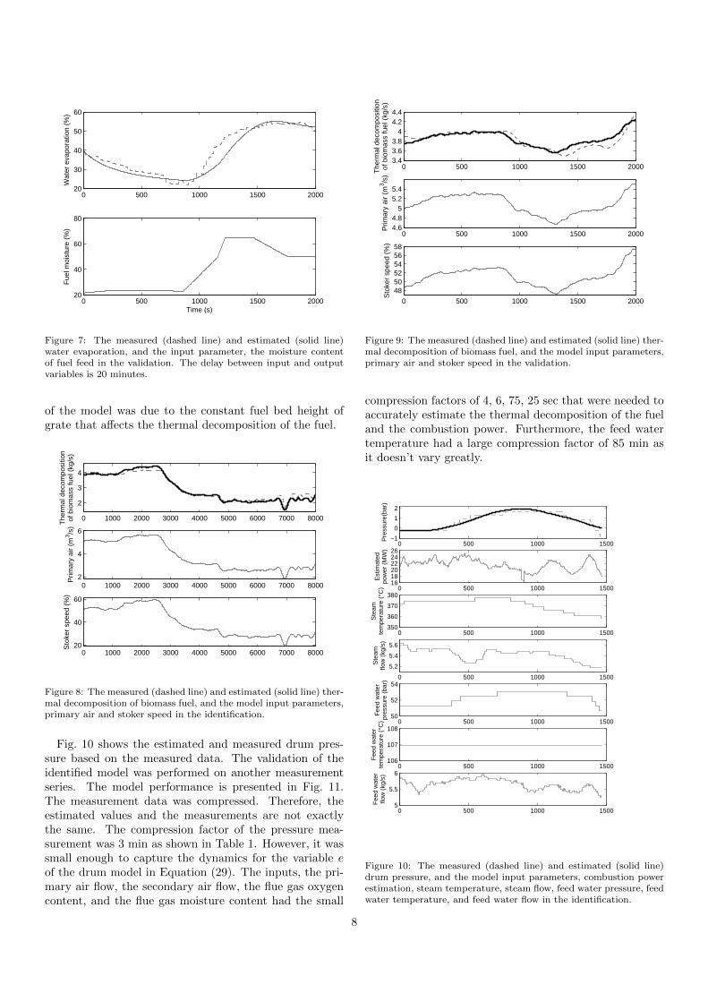
Fig. 10 shows the estimated and measured drum pres-sure based on the measured data. The validation of theidentified model was performed on another measurementseries. The model performance is presented in Fig. 11.The measurement data was compressed. Therefore, theestimated values and the measurements are not exactlythe same. The compression factor of the pressure mea-surement was 3 min as shown in Table 1. However, it wassmall enough to capture the dynamics for the variable eof the drum model in Equation (29). The inputs, the pri-mary air flow, the secondary air flow, the flue gas oxygencontent, and the flue gas moisture content had the small

0 500 1000 1500 20003.43.63.8

44.24.4

The

rmal

dec

ompo

sitio

nof

bio

mas

s fu

el (

kg/s

)

0 500 1000 1500 20004.64.8

55.25.4

Prim

ary

air

(m3 /s

)

0 500 1000 1500 2000

485052545658

Sto

ker

spee

d (%

)

Figure 9: The measured (dashed line) and estimated (solid line) ther-mal decomposition of biomass fuel, and the model input parameters,primary air and stoker speed in the validation.

compression factors of 4, 6, 75, 25 sec that were needed toaccurately estimate the thermal decomposition of the fueland the combustion power. Furthermore, the feed watertemperature had a large compression factor of 85 min asit doesn’t vary greatly.

0 500 1000 1500−1

0

1

2

Pre

ssur

e(ba

r)

0 500 1000 1500161820222426

Est

imat

edpo

wer

(M

W)

0 500 1000 1500350

360

370

380

Ste

amte

mpe

ratu

re (

°C)

0 500 1000 1500

5.2

5.4

5.6

Ste

amflo

w (

kg/s

)

0 500 1000 150050

52

54

Fee

d w

ater

pres

sure

(ba

r)

0 500 1000 1500106

107

108

Fee

d w

ater

tem

pera

ture

(°C

)

0 500 1000 15005

5.5

6

Fee

d w

ater

flow

(kg

/s)

Figure 10: The measured (dashed line) and estimated (solid line)drum pressure, and the model input parameters, combustion powerestimation, steam temperature, steam flow, feed water pressure, feedwater temperature, and feed water flow in the identification.

8

0 500 1000 1500−2

−1

0

Pre

ssur

e(ba

r)

0 500 1000 1500

20

25

30

Est

imat

edpo

wer

(M

W)

0 500 1000 1500350

360

370

380

Ste

amte

mpe

ratu

re (

°C)

0 500 1000 1500

5.25.45.6

Ste

amflo

w (

kg/s

)

0 500 1000 150049

50

51

52

Fee

d w

ater

pres

sure

(ba

r)

0 500 1000 1500106

107

108

Fee

d w

ater

tem

pera

ture

(°C

)

0 500 1000 15005

5.5

6

6.5

Fee

d w

ater

flow

(kg

/s)

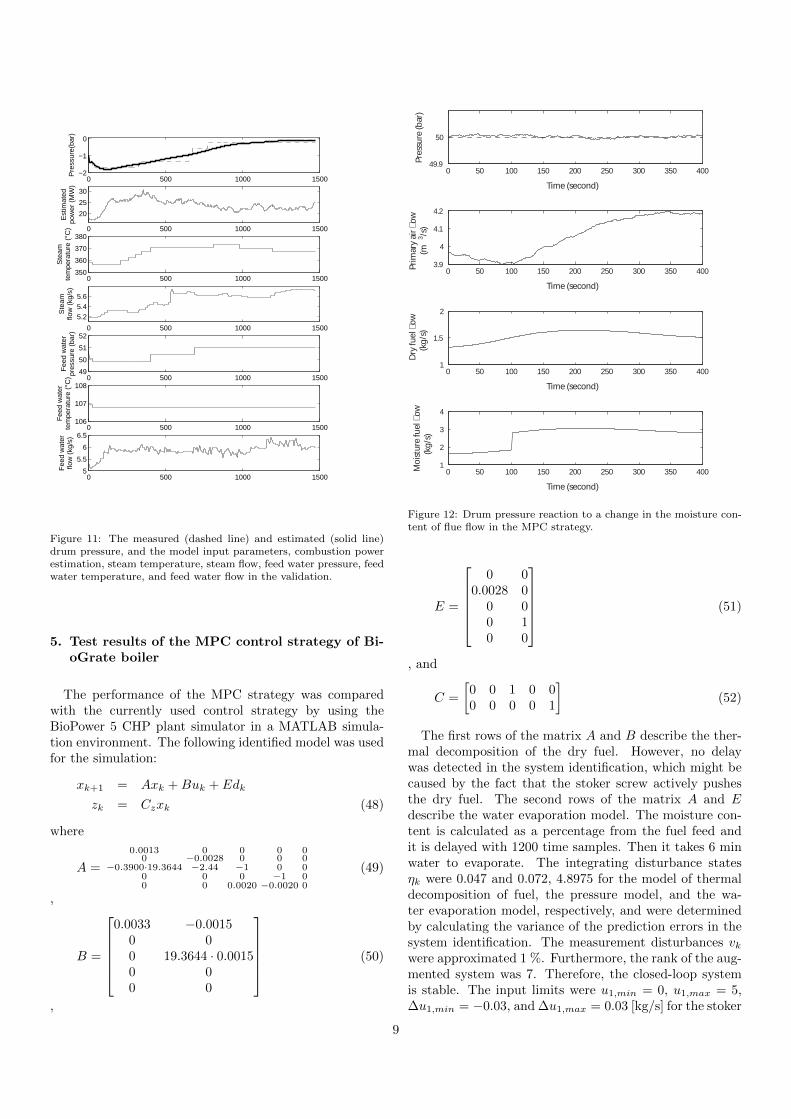
Figure 11: The measured (dashed line) and estimated (solid line)drum pressure, and the model input parameters, combustion powerestimation, steam temperature, steam flow, feed water pressure, feedwater temperature, and feed water flow in the validation.

5. Test results of the MPC control strategy of Bi-oGrate boiler

The performance of the MPC strategy was comparedwith the currently used control strategy by using theBioPower 5 CHP plant simulator in a MATLAB simula-tion environment. The following identified model was usedfor the simulation:

xk+1 = Axk +Buk + Edk

zk = Czxk (48)

where

A =

0.0013 0 0 0 00 −0.0028 0 0 0

−0.3900·19.3644 −2.44 −1 0 00 0 0 −1 00 0 0.0020 −0.0020 0

(49)

,

B =

0.0033 −0.0015

0 00 19.3644 · 0.00150 00 0

(50)

,

0 50 100 150 200 250 300 350 40049.9

50

Pres

sure

(bar

)

Time (second)

0 50 100 150 200 250 300 350 4003.9

4

4.1

4.2

Prim

ary

air �

ow

(

m3 /s

)

Time (second)

0 50 100 150 200 250 300 350 4001

1.5

2

Dry

fuel

�ow

(kg

/s)

Time (second)

0 50 100 150 200 250 300 350 4001

2

3

4M

oist

ure

fuel

�ow

(kg/

s)

Time (second)

Figure 12: Drum pressure reaction to a change in the moisture con-tent of flue flow in the MPC strategy.

E =

0 0

0.0028 00 00 10 0

(51)

, and

C =

[0 0 1 0 00 0 0 0 1

](52)

The first rows of the matrix A and B describe the ther-mal decomposition of the dry fuel. However, no delaywas detected in the system identification, which might becaused by the fact that the stoker screw actively pushesthe dry fuel. The second rows of the matrix A and Edescribe the water evaporation model. The moisture con-tent is calculated as a percentage from the fuel feed andit is delayed with 1200 time samples. Then it takes 6 minwater to evaporate. The integrating disturbance statesηk were 0.047 and 0.072, 4.8975 for the model of thermaldecomposition of fuel, the pressure model, and the wa-ter evaporation model, respectively, and were determinedby calculating the variance of the prediction errors in thesystem identification. The measurement disturbances vkwere approximated 1 %. Furthermore, the rank of the aug-mented system was 7. Therefore, the closed-loop systemis stable. The input limits were u1,min = 0, u1,max = 5,∆u1,min = −0.03, and ∆u1,max = 0.03 [kg/s] for the stoker

9

0 50 100 150 200 250 300 350 40049.5

50

50.5

Pres

sure

(bar

)

Time (second)

0 50 100 150 200 250 300 350 4002

3

4

5

Prim

ary

air �

ow

(m

3 /s)

Time (second)

0 50 100 150 200 250 300 350 4000.5

1

1.5

2

Dry

fuel

�ow

(k

g/s)

Time (second)

0 50 100 150 200 250 300 350 400

12

14

16

18

Stea

m p

ower

(MW

)

Time (second)

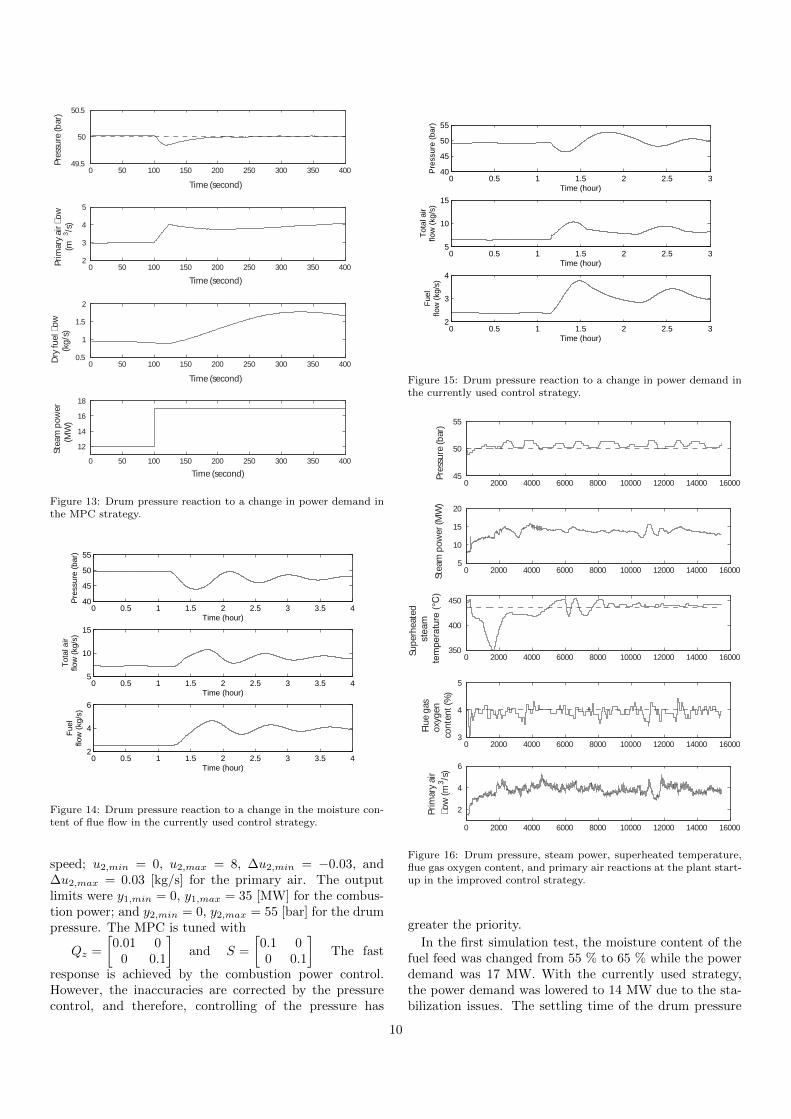
Figure 13: Drum pressure reaction to a change in power demand inthe MPC strategy.

0 0.5 1 1.5 2 2.5 3 3.5 440

45

50

55

Pre

ssur

e (b

ar)

Time (hour)

0 0.5 1 1.5 2 2.5 3 3.5 45

10

15

Tot

al a

irflo

w (

kg/s

)

Time (hour)

0 0.5 1 1.5 2 2.5 3 3.5 42

4

6

Fue

lflo

w (

kg/s

)

Time (hour)

Figure 14: Drum pressure reaction to a change in the moisture con-tent of flue flow in the currently used control strategy.

speed; u2,min = 0, u2,max = 8, ∆u2,min = −0.03, and∆u2,max = 0.03 [kg/s] for the primary air. The outputlimits were y1,min = 0, y1,max = 35 [MW] for the combus-tion power; and y2,min = 0, y2,max = 55 [bar] for the drumpressure. The MPC is tuned with

Qz =

[0.01 0

0 0.1

]and S =

[0.1 00 0.1

]The fast

response is achieved by the combustion power control.However, the inaccuracies are corrected by the pressurecontrol, and therefore, controlling of the pressure has

0 0.5 1 1.5 2 2.5 340

45

50

55

Pre

ssur

e (b

ar)

Time (hour)

0 0.5 1 1.5 2 2.5 35

10

15

Tot

al a

irflo

w (

kg/s

)

Time (hour)

0 0.5 1 1.5 2 2.5 32

3

4

Fue

lflo

w (

kg/s

)

Time (hour)

Figure 15: Drum pressure reaction to a change in power demand inthe currently used control strategy.

0 2000 4000 6000 8000 10000 12000 14000 1600045

50

55

Pres

sure

(bar

)

0 2000 4000 6000 8000 10000 12000 14000 160005

10

15

20

Stea

m p

ower

(MW

)

0 2000 4000 6000 8000 10000 12000 14000 16000350

400

450

Supe

rhea

ted

0 2000 4000 6000 8000 10000 12000 14000 160003

4

5

Flue

gas

ox

ygen

co

nten

t (%

)

0 2000 4000 6000 8000 10000 12000 14000 16000

2

4

6

Prim

ary

air

�ow

(m3 /s

)

Figure 16: Drum pressure, steam power, superheated temperature,flue gas oxygen content, and primary air reactions at the plant start-up in the improved control strategy.

greater the priority.

In the first simulation test, the moisture content of thefuel feed was changed from 55 % to 65 % while the powerdemand was 17 MW. With the currently used strategy,the power demand was lowered to 14 MW due to the sta-bilization issues. The settling time of the drum pressure

10

55

0 2000 4000 6000 8000 10000 12000 14000 1600045

50

Pres

sure

(bar

)

0 2000 4000 6000 8000 10000 12000 14000 160005

10

15

20

Stea

m p

ower

(MW

)

0 2000 4000 6000 8000 10000 12000 14000 16000350

400

450

Supe

rhea

ted

0 2000 4000 6000 8000 10000 12000 14000 160003

4

5

Flue

gas

o

xyge

n c

onte

nt (%

)

0 2000 4000 6000 8000 10000 12000 14000 16000

2

4

6

Prim

ary

air

�ow

(m3 /s

)

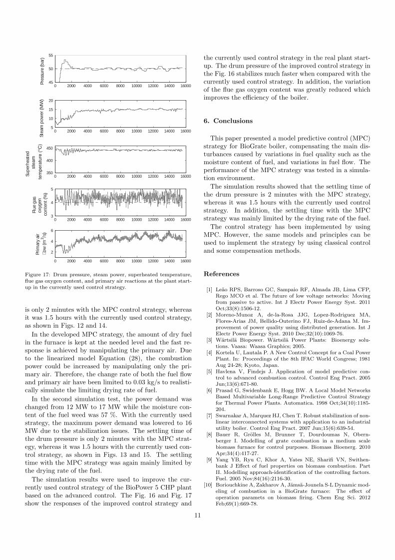
Figure 17: Drum pressure, steam power, superheated temperature,flue gas oxygen content, and primary air reactions at the plant start-up in the currently used control strategy.

is only 2 minutes with the MPC control strategy, whereasit was 1.5 hours with the currently used control strategy,as shown in Figs. 12 and 14.

In the developed MPC strategy, the amount of dry fuelin the furnace is kept at the needed level and the fast re-sponse is achieved by manipulating the primary air. Dueto the linearized model Equation (28), the combustionpower could be increased by manipulating only the pri-mary air. Therefore, the change rate of both the fuel flowand primary air have been limited to 0.03 kg/s to realisti-cally simulate the limiting drying rate of fuel.

In the second simulation test, the power demand waschanged from 12 MW to 17 MW while the moisture con-tent of the fuel weed was 57 %. With the currently usedstrategy, the maximum power demand was lowered to 16MW due to the stabilization issues. The settling time ofthe drum pressure is only 2 minutes with the MPC strat-egy, whereas it was 1.5 hours with the currently used con-trol strategy, as shown in Figs. 13 and 15. The settlingtime with the MPC strategy was again mainly limited bythe drying rate of the fuel.

The simulation results were used to improve the cur-rently used control strategy of the BioPower 5 CHP plantbased on the advanced control. The Fig. 16 and Fig. 17show the responses of the improved control strategy and

the currently used control strategy in the real plant start-up. The drum pressure of the improved control strategy inthe Fig. 16 stabilizes much faster when compared with thecurrently used control strategy. In addition, the variationof the flue gas oxygen content was greatly reduced whichimproves the efficiency of the boiler.

6. Conclusions

This paper presented a model predictive control (MPC)strategy for BioGrate boiler, compensating the main dis-turbances caused by variations in fuel quality such as themoisture content of fuel, and variations in fuel flow. Theperformance of the MPC strategy was tested in a simula-tion environment.

The simulation results showed that the settling time ofthe drum pressure is 2 minutes with the MPC strategy,whereas it was 1.5 hours with the currently used controlstrategy. In addition, the settling time with the MPCstrategy was mainly limited by the drying rate of the fuel.

The control strategy has been implemented by usingMPC. However, the same models and principles can beused to implement the strategy by using classical controland some compensation methods.

References

[1] Leao RPS, Barroso GC, Sampaio RF, Almada JB, Lima CFP,Rego MCO et al. The future of low voltage networks: Movingfrom passive to active. Int J Electr Power Energy Syst. 2011Oct;33(8):1506-12.

[2] Moreno-Munoz A, de-la-Rosa JJG, Lopez-Rodriguez MA,Flores-Arias JM, Bellido-Outerino FJ, Ruiz-de-Adana M. Im-provement of power quality using distributed generation. Int JElectr Power Energy Syst. 2010 Dec;32(10):1069-76.

[3] Wartsila Biopower. Wartsila Power Plants: Bioenergy solu-tions. Vaasa: Waasa Graphics; 2005.

[4] Kortela U, Lautala P. A New Control Concept for a Coal PowerPlant. In: Proceedings of the 8th IFAC World Congress; 1981Aug 24-28; Kyoto, Japan.

[5] Havlena V, Findejs J. Application of model predictive con-trol to advanced combustion control. Control Eng Pract. 2005Jun;13(6):671-80.

[6] Prasad G, Swidenbank E, Hogg BW. A Local Model NetworksBased Multivariable Long-Range Predictive Control Strategyfor Thermal Power Plants. Automatica. 1998 Oct;34(10):1185-204.

[7] Swarnakar A, Marquez HJ, Chen T. Robust stabilization of non-linear interconnected systems with application to an industrialutility boiler. Control Eng Pract. 2007 Jun;15(6):639-54.

[8] Bauer R, Grolles M, Brunner T, Dourdoumas N, Obern-berger I. Modelling of grate combustion in a medium scalebiomass furnace for control purposes. Biomass Bioenerg. 2010Apr;34(4):417-27.

[9] Yang YB, Ryu C, Khor A, Yates NE, Sharifi VN, Swithen-bank J Effect of fuel properties on biomass combustion. PartII. Modelling approach-identification of the controlling factors.Fuel. 2005 Nov;84(16):2116-30.

[10] Boriouchkine A, Zakharov A, Jamsa-Jounela S-L Dynamic mod-eling of combustion in a BioGrate furnace: The effect ofoperation paramets on biomass firing. Chem Eng Sci. 2012Feb;69(1):669-78.

11

[11] Kortela J, Jamsa-Jounela S-L. Fuel-quality soft sensor using thedynamic superheater model for control strategy improvement ofthe BioPower 5 CHP plant. Int J Electr Power Energy Syst. 2012Nov;42(1):38-48.

[12] Maciejowski JM. Predictive Control with Constraints. Harlow,England: Prentice Hal; 2002.

[13] Pannocchia G, Rawlings JB Disturbance Models for Offset-FreeMode-Prodictive Control. AIChE. 2003 Feb;49(2):426-27.

[14] Astrom, KJ, Bell RD. Drum-boiler dynamics. Automatica. 2000Mar;36(3):363-78.

[15] Kortela J, Jamsa-Jounela S-L. Fuel moisture soft-sensor and itsvalidation for the industrial BioPower 5 CHP plant. AppliedEnergy. 2013 May;105:66-74.

12