infinitesimal symmetry transformations of matrix-valued

PART C: Natural Sciences and Mathematics

ISSN:1791-4469 Copyright © 2018, Hellenic Naval Academy

C-31

Infinitesimal symmetry transformations of matrix-valued

differential equations: An algebraic approach

C. J. Papachristou

Department of Physical Sciences, Hellenic Naval Academy, Piraeus 18539, Greece

E-mail: [email protected]

Abstract. The study of symmetries of partial differential equations (PDEs) has been

traditionally treated as a geometrical problem. Although geometrical methods have been

proven effective with regard to finding infinitesimal symmetry transformations, they present

certain conceptual difficulties in the case of matrix-valued PDEs; for example, the usual

differential-operator representation of the symmetry-generating vector fields is not possible in

this case. An algebraic approach to the symmetry problem of PDEs is described, based on

abstract operators (characteristic derivatives) which admit a standard differential-operator

representation in the case of scalar-valued PDEs.

Keywords: Matrix-valued differential equations, symmetry transformations, Lie algebras,

recursion operators

PACS: 02.30.Jr, 02.10.Yn, 02.20.Sv

1. Introduction

The problem of symmetries of a system of partial differential equations (PDEs) has been

traditionally treated as a geometrical problem in the jet space of the independent and the

dependent variables (including a sufficient number of partial derivatives of the latter variables

with respect to the former ones). Two more or less equivalent approaches have been followed:

(a) invariance of the system of PDEs itself, under infinitesimal transformations generated by

corresponding vector fields in the jet space [1]; (b) invariance of a differential ideal of

differential forms representing the system of PDEs, under the Lie derivative with respect to the

vector fields representing the symmetry transformations [2-6].

Although effective with regard to calculating symmetries, these geometrical approaches

suffer from a certain drawback of conceptual nature when it comes to matrix-valued PDEs. The

problem is related to the inevitably mixed nature of the coordinates in the jet space (scalar

independent variables versus matrix-valued dependent ones) and the need for a differential-

operator representation of the symmetry vector fields. How does one define differentiation with

respect to matrix-valued variables? Moreover, how does one calculate the Lie bracket of two

differential operators in which some (or all) of the variables, as well as the coefficients of partial

derivatives with respect to these variables, are matrices?

Although these difficulties were handled in some way in [4-6], it was eventually realized that

an alternative, purely algebraic approach to the symmetry problem would be more appropriate in

the case of matrix-valued PDEs. Elements of this approach were presented in [7] and later

mailto:[email protected]

NAUSIVIOS CHORA, VOL. 7, 2018

http://nausivios.hna.gr/

C-32

applied in particular problems [8-10]; no formal theoretical framework was fully developed,

however.

An attempt to develop such a framework is made in this article. In Sections 2 and 3 we

introduce the concept of the characteristic derivative – an abstract operator generalization of the

Lie derivative used in scalar-valued problems – and we demonstrate the Lie-algebraic nature of

the set of these derivatives.

The general symmetry problem for matrix-valued PDEs is presented in Sec. 4, and the Lie-

algebraic property of symmetries of a PDE is proven in Sec. 5. In Sec. 6 we discuss the concept

of a recursion operator [1,8-14] by which an infinite set of symmetries may in principle be

produced from any known symmetry.

Finally, an application of these ideas is made in Sec. 7 by using the chiral field equation as an

example.

To simplify our formalism, we restrict our analysis to the case of a single matrix-valued PDE

in one dependent variable. Generalization to systems of PDEs is straightforward and is left to the

reader (see, e.g., [1] for scalar-valued problems).

2. Total and characteristic derivative operators

A PDE for the unknown function u=u(x1, x

2, ... ) u(x

k) [where by (x

k) we collectively denote

the independent variables x1, x

2, ...] is an expression of the form F[u]=0, where F[u] F(x

k, u, uk ,

ukl , ...) is a function in the jet space [1] of the independent variables (xk), the dependent variable

u, and the partial derivatives of various orders of u with respect to the xk, which derivatives will

be denoted by using subscripts: uk , ukl , uklm , etc. A solution of the PDE is any function u=φ(xk)

for which the relation F[u]=0 is satisfied at each point (xk) in the domain of φ.

We assume that u, as well as all functions F[u] in the jet space, are square-matrix-valued of

fixed matrix dimensions. In particular, we require that, in its most general form, a function F[u]

in the jet space is expressible as a finite or an infinite sum of products of alternating x-dependent

and u-dependent terms, of the form

[ ] ( ) [ ] ( ) [ ] ( )k k kF u a x u b x u c x (2.1)

where the a(xk), b(x

k), c(x

k), etc., are matrix-valued, and where the matrices Π[u], Π΄[u], etc., are

products of variables u, uk , ukl , etc., of the “fiber” space (or, more generally, products of powers

of these variables). The set of all functions (2.1) is thus a (generally) non-commutative algebra.

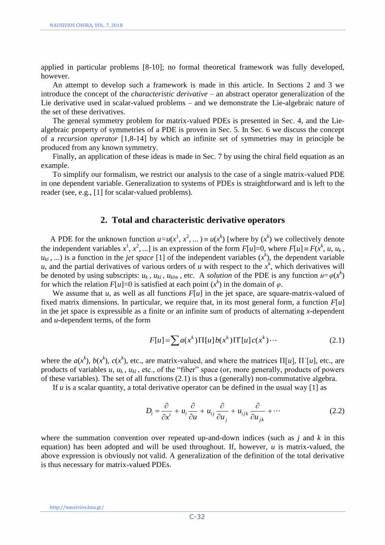
If u is a scalar quantity, a total derivative operator can be defined in the usual way [1] as

i i i j i jkij jk

D u u uu u ux

(2.2)

where the summation convention over repeated up-and-down indices (such as j and k in this

equation) has been adopted and will be used throughout. If, however, u is matrix-valued, the

above expression is obviously not valid. A generalization of the definition of the total derivative

is thus necessary for matrix-valued PDEs.



C-33

Definition 2.1. The total derivative operator with respect to the variable xi is a linear operator

Di acting on functions F[u] of the form (2.1) in the jet space and having the following properties:

1. On functions f (xk) in the base space, Di f (x

k) = f / x

i i f (x

k) .

2. For F[u]=u , ui , uij , etc., we have: Di u = ui , Di uj = Dj ui = uij = uji , etc.

3. The operator Di is a derivation on the algebra of all matrix-valued functions of the form (2.1)

in the jet space; i.e., the Leibniz rule is satisfied:

[ ] [ ] [ ] [ ] [ ] [ ]i i iD F u G u D F u G u F u DG u (2.3)

Higher-order total derivatives Dij=DiDj may similarly be defined but they no longer possess

the derivation property. Given that ij=ji and that uij=uji , it follows that DiDj = DjDi Dij =

Dji ; that is, total derivatives commute. We write: [Di , Dj]=0, where, in general, [A, B] AB–BA

will denote the commutator of two operators or two matrices, as the case may be.

If u–1

is the inverse of u, such that uu–1

= u–1

u = , then we can define

1 1 1i iD u u D u u (2.4)

Moreover, for any functions A[u] and B[u] in the jet space, it can be shown that

[ , ] , ,i i iD A B D A B A D B (2.5)

As an example, let (x1, x

2) (x, t) and let F[u]=xtux

2, where u is matrix-valued. Writing

F[u]=xtuxux , we have: Dt F[u]=xux2

+ xt (uxt ux + ux uxt ).

Let now Q[u] Q (xk, u, uk , ukl , ...) be a function in the jet space. We will call this a

characteristic function (or simply a characteristic) of a certain derivative, defined as follows:

Definition 2.2. The characteristic derivative with respect to Q[u] is a linear operator ΔQ

acting on functions F[u] in the jet space and having the following properties:

1. On functions f (xk) in the base space,

( ) 0kQ f x (2.6)

(that is, ΔQ acts only in the fiber space).

2. For F[u]=u ,

[ ]Qu Q u (2.7)

3. ΔQ commutes with total derivatives:

[ , ] 0 (all )Q i i Q Q iD D D i (2.8)



C-34

4. The operator ΔQ is a derivation on the algebra of all matrix-valued functions of the form (2.1)

in the jet space (the Leibniz rule is satisfied):

[ ] [ ] [ ] [ ] [ ] [ ]Q Q QF u G u F u G u F u G u (2.9)

Corollary: By (2.7) and (2.8) we have:

[ ]Q i Q i iu D u D Q u (2.10)

We note that the operator ΔQ is a well-defined quantity, in the sense that the action of ΔQ on u

uniquely determines the action of ΔQ on any function F[u] of the form (2.1) in the jet space.

Moreover, since, by assumption, u and Q[u] are matrices of equal dimensions, it follows from

(2.7) that ΔQ preserves the matrix character of u, as well as of any function F[u] on which this

operator acts.

We also remark that we have imposed conditions (2.6) and (2.8) having a certain property of

symmetries of PDEs in mind; namely, every symmetry of a PDE can be represented by a

transformation of the dependent variable u alone, i.e., can be expressed as a transformation in the

fiber space (see [1], Chap. 5).

The following formulas, analogous to (2.4) and (2.5), may be written:

1 1 1Q Qu u u u (2.11)

[ , ] , ,Q Q QA B A B A B (2.12)

As an example, let (x1, x

2) (x, t) and let F[u]=a(x,t)u

2b(x,t)+[ux , ut] , where a, b and u are

matrices of equal dimensions. Writing u2=uu and using properties (2.7), (2.9), (2.10) and (2.12),

we find: ΔQ F[u]=a(x,t)(Qu+uQ)b(x,t)+[Dx Q, ut]+[ux , Dt Q].

In the case where u is scalar-valued (thus so is Q[u]), the characteristic derivative ΔQ admits a

differential-operator representation of the form

[ ] [ ] [ ]Q i i j

i i j

Q u D Q u D D Q uu u u

(2.13)

(See [1], Chap. 5, for an analytic proof of property (2.8) in this case.)

3. The Lie algebra of characteristic derivatives

The characteristic derivatives ΔQ acting on functions F[u] of the form (2.1) in the jet space

constitute a Lie algebra of derivations on the algebra of the F[u]. The proof of this statement is

contained in the following three Propositions.



C-35

Proposition 3.1. Let ΔQ be a characteristic derivative with respect to the characteristic Q[u];

i.e., ΔQ u=Q[u] [cf. Eq. (2.7)]. Let λ be a constant (real or complex). We define the operator λΔQ

by the relation

(λΔQ) F[u] λ (ΔQ F[u] ) .

Then, λΔQ is a characteristic derivative with characteristic λQ[u]. That is,

Q Q (3.1)

Proof. (a) The operator λΔQ is linear, since so is ΔQ .

(b) For F[u]=u, (λΔQ)u= λ(ΔQ u)=λQ[u] .

(c) λΔQ commutes with total derivatives Di , since so does ΔQ .

(d) Given that ΔQ satisfies the Leibniz rule (2.9), it is easily shown that so does λΔQ .

Comment: Condition (c) would not be satisfied if we allowed λ to be a function of the xk,

instead of being a constant, since λ(xk) generally does not commute with the Di. Therefore,

relation (3.1) is not valid for a non-constant λ.

Proposition 3.2. Let Δ1 and Δ2 be characteristic derivatives with respect to the characteristics

Q1[u] and Q2[u], respectively; i.e., Δ1u=Q1[u], Δ2u=Q2[u]. We define the operator Δ1+Δ2 by

(Δ1+Δ2) F[u] Δ1 F[u] + Δ2 F[u] .

Then, Δ1+Δ2 is a characteristic derivative with characteristic Q1[u]+Q2[u]. That is,

1 2 1 2with [ ] [ ] [ ]Q Q u Q u Q u (3.2)

Proof. (a) The operator Δ1+Δ2 is linear, as a sum of linear operators.

(b) For F[u]=u, (Δ1+Δ2)u = Δ1u +Δ2u = Q1[u]+Q2[u] .

(c) Δ1+Δ2 commutes with total derivatives Di , since so do Δ1 and Δ2 .

(d) Given that each of Δ1 and Δ2 satisfies the Leibniz rule (2.9), it is not hard to show that the

same is true for Δ1+Δ2 .

Proposition 3.3. Let Δ1 and Δ2 be characteristic derivatives with respect to the characteristics

Q1[u] and Q2[u], respectively; i.e., Δ1u=Q1[u], Δ2u=Q2[u]. We define the operator [Δ1 , Δ2] (Lie

bracket of Δ1 and Δ2) by

[Δ1 , Δ2] F[u] Δ1 (Δ2 F[u]) – Δ2 (Δ1 F[u]) .

Then, [Δ1 , Δ2] is a characteristic derivative with characteristic Δ1Q2[u]–Δ2Q1[u]. That is,

1 2 1 2 2 1 1,2[ , ] with [ ] [ ] [ ] [ ]Q Q u Q u Q u Q u (3.3)



C-36

Proof. (a) The linearity of [Δ1 , Δ2] follows from the linearity of Δ1 and Δ2 .

(b) For F[u]=u, [Δ1 , Δ2]u = Δ1 (Δ2u) – Δ2 (Δ1u) = Δ1Q2[u]–Δ2Q1[u] Q1,2[u] .

(c) [Δ1 , Δ2] commutes with total derivatives Di , since so do Δ1 and Δ2 .

(d) Given that each of Δ1 and Δ2 satisfies the Leibniz rule (2.9), one can show (after some

algebra and cancellation of terms) that the same is true for [Δ1 , Δ2].

In the case where u (thus the Q’s also) is scalar-valued, the Lie bracket admits a standard

differential-operator representation [1]:

1 2 1,2 1,2 1,2[ , ] [ ] i i j

i i j

Q u D Q D D Qu u u

(3.4)

where Q1,2[u] = [Δ1 , Δ2] u = Δ1Q2[u] – Δ2Q1[u] .

The Lie bracket [Δ1 , Δ2] has the following properties:

1. [Δ1 , aΔ2+bΔ3] = a [Δ1 , Δ2] + b [Δ1 , Δ3] ;

[aΔ1+bΔ2 , Δ3] = a [Δ1 , Δ3] + b [Δ2 , Δ3] (a, b = const.)

2. [Δ1 , Δ2] = – [Δ2 , Δ1] (antisymmetry)

3. [Δ1 , [Δ2 , Δ3]] + [Δ2 , [Δ3 , Δ1]] + [Δ3 , [Δ1 , Δ2]] = 0 ;

[[Δ1 , Δ2] , Δ3] + [[Δ2 , Δ3] , Δ1] + [[Δ3 , Δ1] , Δ2] = 0 (Jacobi identity)

4. The symmetry problem for PDEs

Let F[u]=0 be a PDE in the independent variables xk x

1, x

2, ... , and the (generally) matrix-

valued dependent variable u. A transformation u(xk)u΄(x

k) from the function u to a new

function u΄ represents a symmetry of the PDE if the following condition is satisfied: u΄(xk) is a

solution of F[u]=0 when u(xk) is a solution; that is, F[u΄]=0 when F[u]=0.

We will restrict our attention to continuous symmetries, which can be expressed as

infinitesimal transformations. Although such symmetries may involve transformations of the

independent variables (xk), they may equivalently be expressed as transformations of u alone (see

[1], Chap. 5), i.e., as transformations in the fiber space.

An infinitesimal symmetry transformation is written symbolically as

u u΄= u+δu

where δu is an infinitesimal quantity, in the sense that all powers (δu)n with n>1 may be

neglected. The symmetry condition is thus written

F[u+δu] = 0 when F[u] = 0 (4.1)



C-37

An infinitesimal change δu of u induces a change δF[u] of F[u], where

δF[u] = F[u+δu] – F[u] F[u+δu] = F[u] + δF[u] (4.2)

Now, if δu is an infinitesimal symmetry and if u is a solution of F[u]=0, then u+δu also is a

solution; that is, F[u+δu]=0. This means that δF[u]=0 when F[u]=0. The symmetry condition

(4.1) is thus written as follows:

δF[u] = 0 mod F[u] (4.3)

A symmetry transformation (we denote it M) of the PDE F[u]=0 produces a one-parameter

family of solutions of the PDE from any given solution u(xk). We express this by writing

: ( ) ( ; ) with ( ;0) ( )k k k kM u x u x u x u x (4.4)

For infinitesimal values of the parameter α,

0

( ; ) ( ) [ ] where [ ]k k duu x u x Q u Q u

d

(4.5)

The function Q[u] Q(xk, u, uk , ukl , ...) in the jet space is called the characteristic of the

symmetry (or, the symmetry characteristic). Putting

( ; ) ( )k ku u x u x (4.6)

we write, for infinitesimal α,

δu = α Q[u] (4.7)

We notice that the infinitesimal operator δ has the following properties:

1. According to its definition (4.2), δ is a linear operator :

δ(F[u]+G[u]) = (F[u+δu]+ G[u+δu]) – (F[u]+G[u]) = δF[u]+δG[u] .

2. By assumption regarding the nature of our symmetry transformations, δ produces changes in

the fiber space while it doesn’t affect functions f (xk) in the base space [this is implicitly stated in

(4.6)].

3. Since δ represents a difference, it commutes with all total derivatives Di :

δ (Di A[u]) = Di (δA[u]) .

In particular, for A[u]=u,



C-38

δui = δ (Di u) = Di (δu) = α Di Q[u] ,

where we have used (4.7).

4. Since δ expresses an infinitesimal change, it may be approximated to a differential; in

particular, it satisfies the Leibniz rule:

δ (A[u]B[u]) = (δA[u]) B[u] + A[u] δB[u] .

For example, δ(u2) = δ(uu) = (δu)u+uδu = α (Qu+uQ) .

Now, consider the characteristic derivative ΔQ with respect to the symmetry characteristic

Q[u]. According to (2.7),

ΔQ u = Q[u] (4.8)

We observe that the infinitesimal operator δ and the characteristic derivative ΔQ share common

properties. From (4.7) and (4.8) it follows that the two linear operators are related by

δu = α ΔQ u (4.9)

and, by extension,

δui = α Di Q[u] = α ΔQ ui , etc.

[see (2.10)]. Moreover, for scalar-valued u and by the infinitesimal character of the operator δ,

we may write:

[ ] [ ] [ ] [ ]i i i j

i i i j

F F F F FF u u u Q u D Q u D D Q u

u u u u u

while, by (2.13),

[ ] [ ] [ ] [ ]Q i i j

i i j

F F FF u Q u D Q u D D Q u

u u u

(4.10)

The above observations lead us to the conclusion that, in general, the following relation is

true:

δF[u] = α ΔQ F[u] (4.11)

The symmetry condition (4.3) is thus written:

ΔQ F[u] = 0 mod F[u] (4.12)

In particular, if u is scalar-valued, the above condition is written



C-39

[ ] [ ] [ ] 0 mod [ ]i i j

i i j

F F FQ u D Q u D D Q u F u

u u u

(4.13)

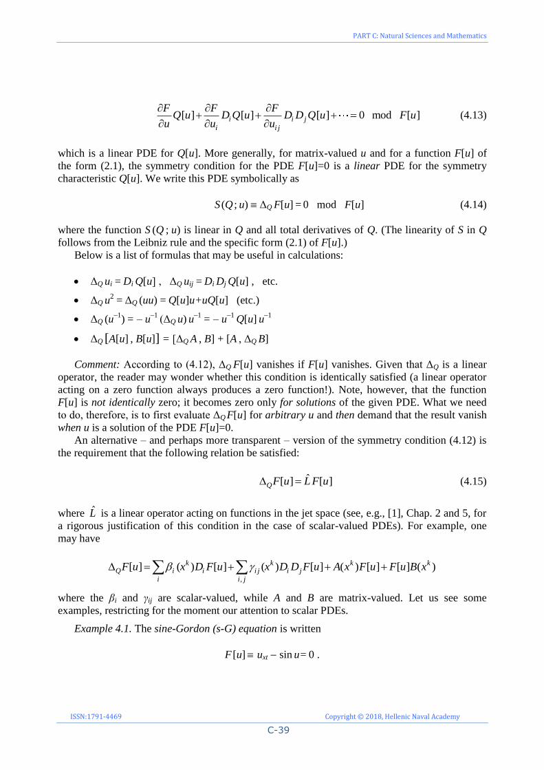
which is a linear PDE for Q[u]. More generally, for matrix-valued u and for a function F[u] of

the form (2.1), the symmetry condition for the PDE F[u]=0 is a linear PDE for the symmetry

characteristic Q[u]. We write this PDE symbolically as

S (Q ; u) ΔQ F[u] = 0 mod F[u] (4.14)

where the function S (Q ; u) is linear in Q and all total derivatives of Q. (The linearity of S in Q

follows from the Leibniz rule and the specific form (2.1) of F[u].)

Below is a list of formulas that may be useful in calculations:

ΔQ ui = Di Q[u] , ΔQ uij = Di Dj Q[u] , etc.

ΔQ u2

= ΔQ (uu) = Q[u]u+uQ[u] (etc.)

ΔQ (u–1

) = – u

–1 (ΔQ u) u

–1 = – u

–1 Q[u] u

–1

ΔQ [A[u] , B[u]] = [ΔQ A , B] + [A , ΔQ B]

Comment: According to (4.12), ΔQ F[u] vanishes if F[u] vanishes. Given that ΔQ is a linear

operator, the reader may wonder whether this condition is identically satisfied (a linear operator

acting on a zero function always produces a zero function!). Note, however, that the function

F[u] is not identically zero; it becomes zero only for solutions of the given PDE. What we need

to do, therefore, is to first evaluate ΔQ F[u] for arbitrary u and then demand that the result vanish

when u is a solution of the PDE F[u]=0.

An alternative – and perhaps more transparent – version of the symmetry condition (4.12) is

the requirement that the following relation be satisfied:

ˆ[ ] [ ]QF u LF u (4.15)

where L̂ is a linear operator acting on functions in the jet space (see, e.g., [1], Chap. 2 and 5, for

a rigorous justification of this condition in the case of scalar-valued PDEs). For example, one

may have

,

[ ] ( ) [ ] ( ) [ ] ( ) [ ] [ ] ( )k k k kQ i i i j i j

i i j

F u x D F u x D D F u A x F u F u B x

where the βi and γij are scalar-valued, while A and B are matrix-valued. Let us see some

examples, restricting for the moment our attention to scalar PDEs.

Example 4.1. The sine-Gordon (s-G) equation is written

F [u] uxt sin u= 0 .



C-40

Here, (x1, x

2) (x, t). Since sinu can be expanded into an infinite series in powers of u, we see that

F[u] has the required form (2.1). Moreover, since u is a scalar function, we can write the

symmetry condition by using (4.13):

S (Q ; u) Qxt – (cosu) Q = 0 mod F [u]

where S(Q; u)= ΔQ F[u] and where by subscripts we denote total differentiations with respect to

the indicated variables. Let us verify the solution Q[u] = ux . This characteristic corresponds to the

symmetry transformation [cf. Eq. (4.4)]

: ( , ) ( , ; ) ( , )M u x t u x t u x t (4.16)

which implies that, if u(x,t) is a solution of the s-G equation, then ( , ) ( , )u x t u x t also is a

solution. We have:

Qxt – (cosu) Q = (ux) xt – (cosu) ux = (uxt sin u) x = Dx F [u] = 0 mod F [u] .

Notice that ΔQF[u] is of the form (4.15), with ˆxL D . Similarly, the characteristic Q[u] = ut

corresponds to the symmetry

: ( , ) ( , ; ) ( , )M u x t u x t u x t (4.17)

That is, if u(x,t) is a solution of the s-G equation, then so is ( , ) ( , )u x t u x t . The symmetries

(4.16) and (4.17) reflect the fact that the s-G equation does not contain the variables x and t

explicitly. (Of course, this equation has many more symmetries which are not displayed here;

see, e.g., [1].)

Example 4.2. The heat equation is written

F [u] ut uxx= 0 .

The symmetry condition (4.13) reads

S (Q ; u) Qt – Qxx = 0 mod F [u]

where S(Q; u)= ΔQ F[u]. As is easy to show, the symmetries (4.16) and (4.17) are valid here, too.

Let us now try the solution Q[u] = u . We have:

Qt Qxx = ut uxx = F [u] = 0 mod F [u] .

This symmetry corresponds to the transformation

: ( , ) ( , ; ) ( , )M u x t u x t e u x t (4.18)

and is a consequence of the linearity of the heat equation.



C-41

Example 4.3. One form of the Burgers equation is

F [u] ut uxx ux2

= 0 .

The symmetry condition (4.13) is written

S (Q ; u) Qt Qxx – 2uxQx = 0 mod F [u]

where, as always, S(Q; u)=ΔQ F[u]. Putting Q= ux and Q= ut , we verify the symmetries (4.16)

and (4.17):

Qt Qxx – 2uxQx = uxt – uxxx – 2uxuxx = Dx F [u] = 0 mod F [u]

Qt Qxx – 2uxQx = utt – uxxt – 2uxuxt = Dt F [u] = 0 mod F [u]

Note again that ΔQF[u] is of the form (4.15), with ˆxL D and ˆ tL D . Another symmetry is Q

[u]=1, which corresponds to the transformation

: ( , ) ( , ; ) ( , )M u x t u x t u x t (4.19)

and is a consequence of the fact that u enters F [u] only through its derivatives.

Example 4.4. The wave equation is written

F [u] utt c2

uxx = 0 ( c = const.)

and its symmetry condition reads

S (Q ; u) Qtt c2

Qxx = 0 mod F [u] .

The solution Q[u] = x ux+ t ut corresponds to the symmetry transformation

: ( , ) ( , ; ) ( , )M u x t u x t u e x e t (4.20)

expressing the invariance of the wave equation under a scale change of x and t . [The reader may

show that the transformations (4.16) – (4.19) also express symmetries of the wave equation.]

It is remarkable that each of the above PDEs admits an infinite set of symmetry

transformations [1]. An effective method for finding such infinite sets is the use of a recursion

operator, which produces a new symmetry characteristic every time it acts on a known

characteristic. More will be said on recursion operators in Sec. 6.

5. The Lie algebra of symmetries

As is well known [1], the set of symmetries of a PDE F[u]=0 has the structure of a Lie

algebra. Let us demonstrate this property in the context of our abstract formalism.



C-42

Proposition 5.1. Let be the set of characteristic derivatives ΔQ with respect to the symmetry

characteristics Q[u] of the PDE F[u]=0. The set is a (finite- or infinite-dimensional) Lie

subalgebra of the Lie algebra of characteristic derivatives acting on functions F[u] in the jet

space (cf. Sec. 3).

Proof. (a) Let ΔQ ΔQ F[u]=0 (mod F[u]). If λ is a constant (real or complex, depending

on the nature of the problem) then (λΔQ)F[u] λΔQ F[u]=0, which means that λΔQ. Given that

λΔQ = ΔλQ [see Eq. (3.1)] we conclude that, if Q[u] is a symmetry characteristic of F[u]=0, then

so is λQ[u].

(b) Let Δ1 and Δ2 be characteristic derivatives with respect to the symmetry characteristics

Q1[u] and Q2[u], respectively. Then, Δ1F[u]=0, Δ2F[u]=0, and hence, (Δ1+Δ2)F[u]

Δ1F[u]+Δ2F[u]=0; therefore, (Δ1+Δ2). It also follows from Eq. (3.2) that, if Q1[u] and Q2[u]

are symmetry characteristics of F[u]=0, then so is their sum Q1[u]+Q2[u].

(c) Let Δ1 and Δ2, as above. Then, by (4.15),

1 1ˆ[ ] [ ]F u L F u , 2 2

ˆ[ ] [ ]F u L F u .

Now, by the definition of the Lie bracket and the linearity of both Δi and ˆiL (i=1,2) we have:

1 2 1 2 2 1 1 2 2 1

1 2 2 1

ˆ ˆ[ , ] [ ] ( [ ]) ( [ ]) ( [ ]) ( [ ])

ˆ ˆ( ) [ ] 0 mod [ ]

F u F u F u L F u L F u

L L F u F u

We thus conclude that [Δ1 , Δ2]. Moreover, it follows from Eq. (3.3) that, if Q1[u] and Q2[u]

are symmetry characteristics of F[u]=0, then so is the function

Q1,2 [u] = Δ1 Q2[u] – Δ2 Q1[u] .

Assume now that the PDE F[u]=0 has an n-dimensional symmetry algebra (which may be

a finite subalgebra of an infinite-dimensional symmetry Lie algebra). Let {Δ1 , Δ2 , ... , Δn}{Δk},

with corresponding symmetry characteristics {Qk}, be a set of n linearly independent operators

that constitute a basis of , and let Δi , Δj be any two elements of this basis. Given that [Δi ,

Δj], this Lie bracket must be expressible as a linear combination of the {Δk}, with constant

coefficients. We write

1

[ , ]n

ki j i j k

k

c

(5.1)

where the coefficients of the Δk in the sum are the antisymmetric structure constants of the Lie

algebra in the basis {Δk}.



C-43

The operator relation (5.1) can be expressed in an equivalent, characteristic form by allowing

the operators on both sides to act on u and by using the fact that Δku=Qk[u]:

1 1

[ , ] ( )n n

k ki j i j k i j k

k k

u c u c u

1

[ ] [ ] [ ]n

ki j j i i j k

k

Q u Q u c Q u

(5.2)

Example 5.1. One of the several forms of the Korteweg-de Vries (KdV) equation is

F [u] ut + uux + uxxx = 0 .

The symmetry condition (4.14) is written

S (Q ; u) Qt + Q ux + u Qx + Qxxx = 0 mod F [u] (5.3)

where S(Q; u)= ΔQ F[u]. The KdV equation admits a symmetry Lie algebra of infinite dimensions

[1]. This algebra has a finite, 4-dimensional subalgebra of point transformations. A symmetry

operator (characteristic derivative) ΔQ is determined by its corresponding characteristic Q[u]=ΔQ

u . Thus, a basis {Δ1 ,..., Δ4} of corresponds to a set of four independent characteristics {Q1 ,...,

Q4}. Such a basis of characteristics is the following:

Q1[u]= ux , Q2[u]= ut , Q3[u]= tux – 1 , Q4[u]= xux +3tut + 2u

The Q1 ,..., Q4 satisfy the PDE (5.3), since, as we can show,

S (Q1 ; u) = Dx F [u] , S (Q2 ; u) = Dt F [u] , S (Q3 ; u) = t Dx F [u] ,

S (Q4 ; u) = (5 + x Dx + 3t Dt ) F [u]

[Note once more that ΔQF[u] is of the form (4.15) in each case.] Let us now see two examples of

calculating the structure constants of by application of (5.2). We have:

1 2 2 1 1 2 1 2 1 2

4

121

Δ Δ Δ Δ (Δ ) (Δ ) ( ) ( ) ( ) ( ) 0t x t x t x x t t x

kk

k

Q Q u u u u Q Q u u

c Q

Since the Qk are linearly independent, we must necessarily have 12 0 , 1,2,3,4kc k . Also,

2 3 3 2 2 3 2 3 2 3

4

1 231

Δ Δ Δ ( 1) Δ (Δ ) (Δ ) ( ) ( )

( )

x t x t x t

kt x x xt x k

k

Q Q tu u t u u t Q Q

tu u tu u Q c Q



C-44

Therefore, 1 2 3 423 23 23 231 , 0c c c c .

6. Recursion operators

Let δu=αQ[u] be an infinitesimal symmetry of the PDE F[u]=0, where Q[u] is the symmetry

characteristic. For any solution u(xk) of this PDE, the function Q[u] satisfies the linear PDE

S (Q ; u) ΔQ F[u] = 0 (6.1)

Because of the linearity of (6.1) in Q, the sum Q1[u]+Q2[u] of two solutions of this PDE, as well

as the multiple λQ[u] of any solution by a constant, also are solutions of (6.1) for a given u. Thus,

for any solution u of F[u]=0, the solutions {Q[u]} of the PDE (6.1) form a linear space, which we

call Su .

A recursion operator R̂ is a linear operator that maps the space Su into itself. Thus, if Q[u] is

a symmetry characteristic of F[u]=0 (i.e., a solution of (6.1) for a given u) then so is ˆ [ ]RQ u :

ˆ( ; ) 0 when ( ; ) 0S RQ u S Q u (6.2)

Obviously, any power of a recursion operator also is a recursion operator. Thus, starting with any

symmetry characteristic Q[u], one may in principle obtain an infinite set of such characteristics

by repeated application of the recursion operator.

A new approach to recursion operators was suggested in the early 1990s [11,15-17] (see also

[8-10]) according to which a recursion operator may be viewed as an auto-Bäcklund

transformation (BT) [18] for the symmetry condition (6.1) of the PDE F[u]=0. By integrating the

BT, one obtains new solutions Q΄[u] of the linear PDE (6.1) from known ones, Q[u]. Typically,

this type of recursion operator produces nonlocal symmetries in which the symmetry

characteristic depends on integrals (rather than derivatives) of u. This approach proved to be

particularly effective for matrix-valued PDEs such as the nonlinear self-dual Yang-Mills

equation, of which new infinite-dimensional sets of “potential symmetries” were discovered

[9,11,15].

7. An example: The chiral field equation

Let us consider the chiral field equation

1 1[ ] ( ) ( ) 0x x t tF g g g g g (7.1)

where, in general, subscripts x and t denote total derivatives Dx and Dt , respectively, and where g

is a GL(n,C)-valued function of x and t, i.e., a complex, non-singular (nn) matrix function,

differentiable for all x and t. Let δg=αQ[g] be an infinitesimal symmetry transformation for the

PDE (7.1), with symmetry characteristic Q[g]=ΔQ g . It is convenient to put



C-45

Q[g] = g Φ[g] Φ[g] = g–1

Q[g] .

The symmetry condition for (7.1) is

ΔQ F[g] = 0 mod F[g] .

This condition will yield a linear PDE for Q or, equivalently, a linear PDE for Φ. By using the

properties of the characteristic derivative, we find the latter PDE to be

1 1( ; ) [ , ] [ , ] 0 mod [ ]x x x t t tS g D g g D g g F g (7.2)

where, as usual, square brackets denote commutators of matrices.

A useful identity that will be needed in the sequel is the following:

1 1 1 1( ) ( ) [ , ] 0t x x t x tg g g g g g g g (7.3)

Let us first consider symmetry transformations in the base space, i.e., coordinate

transformations of x, t. An obvious symmetry is x-translation, x΄=x+α, given that the PDE (7.1)

does not contain the independent variable x explicitly. For infinitesimal values of the parameter

α, we write δx=α. The symmetry characteristic is Q[g]=gx , so that Φ[g]=g–1

gx . By substituting

this expression for Φ into the symmetry condition (7.2) and by using the identity (7.3), we can

verify that (7.2) is indeed satisfied:

S (Φ ; g) = Dx F[g] = 0 mod F[g] .

Similarly, for t-translation, t΄=t+α (infinitesimally, δt=α) with Q[g]=gt , we find

S (Φ ; g) = Dt F[g] = 0 mod F[g] .

Another obvious symmetry of (7.1) is a scale change of both x and t : x΄=λx, t΄=λt. Setting

λ=1+α, where α is infinitesimal, we write δx=αx, δt=αt. The symmetry characteristic is

Q[g]=xgx+tgt , so that Φ[g]=xg–1

gx+tg–1

gt . Substituting for Φ into the symmetry condition (7.2)

and using the identity (7.3) where necessary, we find that

S (Φ ; g) = (2 + x Dx + t Dt ) F[g] = 0 mod F[g] .

Let us call Q1[g]=gx , Q2[g]=gt , Q3[g]=xgx+tgt , and let us consider the corresponding

characteristic derivative operators Δi defined by Δi g=Qi (i=1,2,3). It is then straightforward to

verify the following commutation relations:

[Δ1 , Δ2] g = Δ1 Q2 – Δ2 Q1 = 0 [Δ1 , Δ2] = 0 ;

[Δ1 , Δ3] g = Δ1 Q3 – Δ3 Q1 = – gx = – Q1 = – Δ1 g [Δ1 , Δ3] = – Δ1 ;



C-46

[Δ2 , Δ3] g = Δ2 Q3 – Δ3 Q2 = – gt = – Q2 = – Δ2 g [Δ2 , Δ3] = – Δ2 .

Next, we consider the “internal” transformation (i.e., transformation in the fiber space)

g΄=gΛ, where Λ is a non-singular constant matrix. Then,

F[g΄ ] = Λ–1 F[g] Λ = 0 mod F[g] ,

which indicates that this transformation is a symmetry of (7.1). Setting Λ=1+αM, where α is an

infinitesimal parameter while M is a constant matrix, we write, in infinitesimal form, δg=αgM.

The symmetry characteristic is Q[g]=gM, so that Φ[g]=M. Substituting for Φ into the symmetry

condition (7.2), we find:

S (Φ ; g) = [F[g] , M ] = 0 mod F[g] .

Given a matrix function g(x,t) satisfying the PDE (7.1), consider the following system of

PDEs for two functions Φ[g] and Φ΄[g]:

1

1

[ , ]

[ , ]

x t t

t x x

g g

g g

(7.4)

The integrability condition (or consistency condition) ( ) ( )x t t x of this system requires that

Φ satisfy the symmetry condition (7.2); i.e., S (Φ ; g)=0. Conversely, by applying the integrability

condition ( ) ( )t x x t and by using the fact that g is a solution of F[g]=0, one finds that Φ΄

must also satisfy (7.2); i.e., S (Φ΄; g) = 0.

We conclude that, for any function g(x,t) satisfying the PDE (7.1), the system (7.4) is an

auto-Bäcklund transformation (BT) [18] relating solutions Φ and Φ΄ of the symmetry condition

(7.2) of this PDE; that is, relating different symmetries of the chiral field equation. Thus, if a

symmetry characteristic Q=gΦ of the PDE (7.1) is known, a new characteristic Q΄=gΦ΄ may be

found by integrating the BT (7.4); the converse is also true. Since the BT (7.4) produces new

symmetries from old ones, it may be regarded as a recursion operator for the PDE (7.1) [8-

11,15-17].

As an example, consider the internal-symmetry characteristic Q[g]=gM (where M is a

constant matrix) corresponding to Φ[g]=M. By integrating the BT (7.4) for Φ΄, we get Φ΄=[X, M]

and thus Q΄=g[X, M], where X is the “potential” of the PDE (7.1), defined by the system of PDEs

1 1,x t t xX g g X g g (7.5)

Note the nonlocal character of the BT-produced symmetry Q΄, due to the presence of the

potential X. Indeed, as seen from (7.5), in order to find X one has to integrate the chiral field g

with respect to the independent variables x and t. The above process can be continued

indefinitely by repeated application of the recursion operator (7.4), leading to an infinite

sequence of increasingly nonlocal symmetries.

Unfortunately, as the reader may check, no new information is furnished by the BT (7.4) in

the case of coordinate symmetries (for example, by applying the BT for Q=gx we get the known



C-47

symmetry Q΄=gt ). A recursion operator of the form (7.4), however, does produce new nonlocal

symmetries from coordinate symmetries in related problems with more than two independent

variables, such as the self-dual Yang-Mills equation [8-11,15].

8. Concluding remarks

The algebraic approach to the symmetry problem of PDEs, presented in this article, is, in a

sense, an extension to matrix-valued problems of the ideas contained in [1], in much the same

way as [4] and [5] constitute a generalization of the Harrison-Estabrook geometrical approach [2]

to matrix-valued (as well as vector-valued and Lie-algebra-valued) PDEs. The main advantage of

the algebraic approach is the bypassing of the difficulty associated with the differential-operator

representation of the symmetry-generating vector fields that act on matrix-valued functions in the

jet space.

It should be noted, however, that the standard methods [1,4,5] are still most effective for

calculating symmetries of PDEs. In this regard, one needs to enrich the ideas presented in this

article by describing a systematic process for evaluating (not just recognizing) symmetries, in the

spirit of [4,5]. This will be the subject of a subsequent article.

References

1. P. J. Olver, Applications of Lie Groups to Differential Equations (Springer-Verlag, 1993).

2. B. K. Harrison, F. B. Estabrook, Geometric approach to invariance groups and solutions of

partial differential equations, J. Math. Phys. 12 (1971) 653.

3. D. G. B. Edelen, Applied Exterior Calculus (Wiley, 1985).

4. C. J. Papachristou, B. K. Harrison, Isogroups of differential ideals of vector-valued differential

forms: Application to partial differential equations, Acta Appl. Math. 11 (1988) 155.

5. C. J. Papachristou, B. K. Harrison, Some aspects of the isogroup of the self-dual Yang-Mills

system, J. Math. Phys. 28 (1987) 1261.

6. C. J. Papachristou, B. K. Harrison, Nonlocal symmetries and Bäcklund transformations for the

self-dual Yang-Mills system, J. Math. Phys. 29 (1988) 238.

7. C. J. Papachristou, Symmetry and integrability of classical field equations, arXiv:0803.3688

(http://arxiv.org/abs/0803.3688).

8. C. J. Papachristou, Symmetry, conserved charges, and Lax representations of nonlinear field

equations: A unified approach, Electron. J. Theor. Phys. 7, No. 23 (2010) 1

(http://www.ejtp.com/articles/ejtpv7i23p1.pdf).

9. C. J. Papachristou, B. K. Harrison, Bäcklund-transformation-related recursion operators:

Application to the self-dual Yang-Mills equation, J. Nonlin. Math. Phys., Vol. 17, No. 1 (2010)

35.

10. C. J. Papachristou, Symmetry and integrability of a reduced, 3-dimensional self-dual gauge field

model, Electron. J. Theor. Phys. 9, No. 26 (2012) 119.

(http://www.ejtp.com/articles/ejtpv9i26p119.pdf).

http://arxiv.org/abs/0803.3688

http://www.ejtp.com/articles/ejtpv7i23p1.pdf

http://www.ejtp.com/articles/ejtpv9i26p119.pdf



C-48

11. C. J. Papachristou, Lax pair, hidden symmetries, and infinite sequences of conserved currents for

self-dual Yang-Mills fields, J. Phys. A 24 (1991) L 1051.

12. M. Marvan, A. Sergyeyev, Recursion operators for dispersionless integrable systems in any

dimension, Inverse Problems 28 (2012) 025011.

13. S. Igonin, M. Marvan, On construction of symmetries and recursion operators from zero-

curvature representations and the Darboux–Egoroff system, J. Geom. Phys. 85 (2014) 106.

14. A. Sergyeyev, A simple construction of recursion operators for multidimensional dispersionless

integrable systems, J. Math. Anal. Appl. 454 (2017) 468.

15. C. J. Papachristou, Potential symmetries for self-dual gauge fields, Phys. Lett. A 145 (1990) 250.

16. G. A. Guthrie, Recursion operators and non-local symmetries, Proc. R. Soc. Lond. A 446 (1994)

107.

17. M. Marvan, Another look on recursion operators, in Differential Geometry and Applications

(Proc. Conf., Brno, 1995) 393.

18. C. J. Papachristou, A. N. Magoulas, Bäcklund transformations: Some old and new perspectives,

Nausivios Chora Vol. 6 (2016) pp. C3-C17 (http://nausivios.snd.edu.gr/docs/2016C.pdf).

http://nausivios.snd.edu.gr/docs/2016C.pdf

infinitesimal symmetry transformations of matrix-valued

Documents