implementation of mechanistic pavement design: field … · implementation of mechanistic pavement...

Implementation of Mechanistic Pavement Design:

Field and Laboratory Implementation

FINAL REPORT December 2005

Submitted by

ELF-RU7072

Dr. Ali Maher* Professor and Head

Dr. Nenad Gucunski* Professor

* Center for Advanced Infrastructure & Transportation (CAIT) Rutgers, The State University Piscataway, NJ 08854-8014

* Mr. Thomas Bennert, Research Engineer

In cooperation with

U.S. Department of Transportation Federal Highway Administration

1. Report No. 2. Government Accession No.

TECHNICAL REPORT STANDARD TITLE PAGE

3. Rec ip ient ’s Cata log No.

5 . Repor t Date

8. Performing Organization Report No.

6. Performing Organizat ion Code

4. Ti t le and Subt i t le

7. Author(s)

9. Performing Organization Name and Address 10. Work Unit No.

11. Contract or Grant No.

13. Type of Report and Period Covered

14. Sponsoring Agency Code

12. Sponsoring Agency Name and Address

15. Supplementary Notes

16. Abstract

17. Key Words

19. Security Classif (of this report)

Form DOT F 1700.7 (8-69)

20. Security Classif. (of this page)

18. Distribution Statement

21. No of Pages 22. Price

December 2005

CAIT/Rutgers

Final Report 1/1/2002-12/31/2005

ELF-RU7072

Center for Advanced Infrastructure & Transportation (CAIT) Civil & Environmental Engineering Rutgers, The State University Piscataway, NJ 08854-8014

U.S. Department of Transportation Research & Innovative Technology Administration (RITA) 400 7th Street, SW Washington, DC 20590-0001

One of the most important parameters needed for 2002 Mechanistic Pavement Design Guide is the dynamic modulus (E*). The dynamic modulus (E*) describes the relationship between stress and strain for a linear viscoelastic material. The E* is the prime material parameter used for calculating both rutting and fatigue cracking in hot mix asphalt. The parameter is traditionally measured in the laboratory under an axial compressive type testing condition. Under the recommendations of the 2002 Mechanistic Design Guide, this is the preferred method for reconstruction or new construction. However, if a rehabilitation is to be conducted, the 2002 Mechanistic Design Guide prefers the use of the Falling Weight Deflectometer (FWD) because of its capability of determining the E* parameter in-situ and in a non-destructive way. Unfortunately, this is not 100% true since most PMS procedures require that cores of the pavement be taken so accurate layer thickness’ can be determined for back-calculation purposes. If FWD testing is not available, then the 2002 Mechanistic Design Guide recommends using the laboratory testing of cores from the pavement. Research showed that shear modulus testing (G*) from the Superpave Shear Tester provides modulus values from readily attained cores. The 50 mm samples required by the SST can easily be cut from 6 inch diameter cores. However, as indicated, the G* values obtained can not be directly used in the 2002 Mechanistic Pavement Design Guide without using an assumed Poisson’s Ratio and elastic theory concepts that relate G* to E* (Dynamic Modulus). Intact cores can be taken and trimmed to provide dynamic modulus test specimens, as long as the asphalt pavement thickness is greater than 6 inches thick. A Master Stiffness Curve can then be developed using the E* data determined at various test temperatures and loading frequencies and shifted to the in-situ asphalt pavement temperature. In all test sections evaluated in the study, the Falling Weight Deflectometer (FWD) back-calculated asphalt modulus showed excellent correlation the corresponding Master Stiffness Curve, when it was assumed that the loading frequency of the FWD is 16.7 hertz. This illustrates that if field testing is not available, cores can be taken and tested using the dynamic modulus testing protocol to provide reasonable estimates of the asphalt modulus. And, although further validation is required, the generated Master Stiffness Curve should provide a reasonable estimate of the seasonal variation in asphalt modulus, which would required the FWD to test the identical location at least once every month of a full year.

Dynamic Modulus, Falling Weight Deflectometer, Frequency Sweep, Master Stiffness Curve

Unclassified Unclassified

36

ELF-RU7072

Dr. Ali Maher, Dr. Nenad Gucunski, and Mr. Thomas Bennert

Implementation of Mechanistic Pavement Design: Field and Laboratory Implementation

1

TABLE OF CONTENTS Page # ABSTRACT ..................................................................................................................... 3 INTRODUCTION............................................................................................................. 4

Mechanistic Testing of Modulus .................................................................................. 5 Superpave Shear Tester .......................................................................................... 5 Dynamic Modulus (E*) ............................................................................................. 8 Falling Weight Deflectometer ................................................................................. 10

RESEARCH OBJECTIVES ........................................................................................... 17 EXPERIMENTAL PROGRAM ....................................................................................... 17

FAA NAPTF............................................................................................................... 18 Volumetric Properties of Core Samples ................................................................. 18 Shear Modulus (G*) Test Results........................................................................... 19 Dynamic Modulus (E*) Test Results....................................................................... 23 Comparison of FWD Modulus and Dynamic Modulus............................................ 25

New Jersey State Route 18 ....................................................................................... 27 New Jersey State Route 202 ..................................................................................... 30

CONCLUSIONS............................................................................................................ 33 REFERENCES.............................................................................................................. 34

2

LIST OF FIGURES Figure 1. Superpave Shear Tester (SST) at the Rutgers University Asphalt/Pavement Laboratory Figure 2. HMA Sample Instrumented for the Dynamic Modulus Test Figure 3. Sinusoidal Stress Wave Form Applied During the Dynamic Modulus Test Figure 4. Typical Force Output of FWD Figure 5. Typical Location of Loading Plates and Deflection Sensors for FWD Figure 6. Shear Modulus (G*) Test Results from the Frequency Sweep at Constant

Height Test (FSCH) Figure 7. Viscosity-Temperature Relationship Developed from Extracted Asphalt Binder Figure 8. Master Shear Stiffness Curve for Sample G1 Figure 9. Master Shear Stiffness Curve for Sample G2 Figure 10. Dynamic Modulus (E*) Test Results Figure 11. Master Stiffness Curve for Sample E1 Figure 12. Master Stiffness Curve for Sample E2 Figure 13. Master Stiffness Curve for Sample E3 Figure 14. Master Stiffness Curve and FWD Modulus for Location/Sample E1 Figure 15. Master Stiffness Curve and FWD Modulus for Location/Sample E2 Figure 16. Master Stiffness Curve and FWD Modulus for Location/Sample E3 Figure 17. Dynamic Modulus Sample from NJ Route 18 Figure 18. Graduate Student at Dynamic Modulus Test Set-up Figure 19. Failed Sample During 130oF Test Temperature Figure 20. Master Stiffness Curve and FWD Modulus for MP 7.0 Figure 21. Master Stiffness Curve and FWD Modulus for MP 8.0 Figure 22. Dynamic Modulus Sample from NJ Route 202 Prior to Testing Figure 23. Master Stiffness Curve and FWD Modulus for MP 1.0 Figure 24. Master Stiffness Curve and FWD Modulus for MP 3.0 Figure 25. Master Stiffness Curve and FWD Modulus for MP 5.0 LIST OF TABLES Table I. Recommended Testing for New Construction/Reconstruction Table 2. Significant Features of ASTM D4695 for FWD Testing Table 3. Summary of Differences Calculated and Target Elastic Modulus as a Function of Layer Type Table 4. Summary of Aggregate Bulk Specific Gravity Aggregate Properties Table 5. Volumetric Properties of Test Specimens of NAPTF Table 6. Typical A and VTS Properties of PG Graded Asphalt Binders Table 7. Typical A and VTS Properties of AC Graded Asphalt Binders

3

ABSTRACT One of the most important parameters needed for 2002 Mechanistic Pavement Design Guide is the dynamic modulus (E*). The dynamic modulus (E*) describes the relationship between stress and strain for a linear viscoelastic material. The E* is the prime material parameter used for calculating both rutting and fatigue cracking in hot mix asphalt. The parameter is traditionally measured in the laboratory under an axial compressive type testing condition. Under the recommendations of the 2002 Mechanistic Design Guide, this is the preferred method for reconstruction or new construction. However, if a rehabilitation is to be conducted, the 2002 Mechanistic Design Guide prefers the use of the Falling Weight Deflectometer (FWD) because of its capability of determining the E* parameter in-situ and in a non-destructive way. Unfortunately, this is not 100% true since most PMS procedures require that cores of the pavement be taken so accurate layer thickness’ can be determined for back-calculation purposes. If FWD testing is not available, then the 2002 Mechanistic Design Guide recommends using the laboratory testing of cores from the pavement. Research showed that shear modulus testing (G*) from the Superpave Shear Tester provides modulus values from readily attained cores. The 50 mm samples required by the SST can easily be cut from 6 inch diameter cores. However, as indicated, the G* values obtained can not be directly used in the 2002 Mechanistic Pavement Design Guide without using an assumed Poisson’s Ratio and elastic theory concepts that relate G* to E* (Dynamic Modulus). Intact cores can be taken and trimmed to provide dynamic modulus test specimens, as long as the asphalt pavement thickness is greater than 6 inches thick. A Master Stiffness Curve can then be developed using the E* data determined at various test temperatures and loading frequencies and shifted to the in-situ asphalt pavement temperature. In all test sections evaluated in the study, the Falling Weight Deflectometer (FWD) back-calculated asphalt modulus showed excellent correlation the corresponding Master Stiffness Curve, when it was assumed that the loading frequency of the FWD is 16.7 hertz. This illustrates that if field testing is not available, cores can be taken and tested using the dynamic modulus testing protocol to provide reasonable estimates of the asphalt modulus. And, although further validation is required, the generated Master Stiffness Curve should provide a reasonable estimate of the seasonal variation in asphalt modulus, which would required the FWD to test the identical location at least once every month of a full year.

4

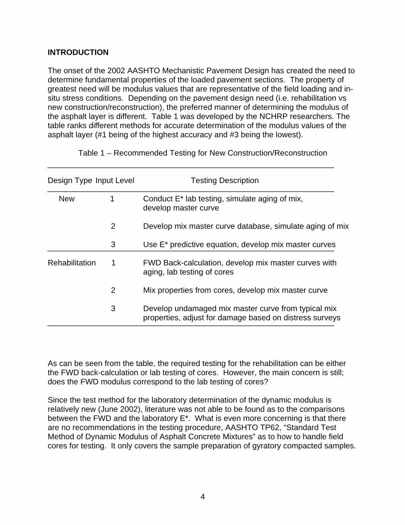
INTRODUCTION The onset of the 2002 AASHTO Mechanistic Pavement Design has created the need to determine fundamental properties of the loaded pavement sections. The property of greatest need will be modulus values that are representative of the field loading and in-situ stress conditions. Depending on the pavement design need (i.e. rehabilitation vs new construction/reconstruction), the preferred manner of determining the modulus of the asphalt layer is different. Table 1 was developed by the NCHRP researchers. The table ranks different methods for accurate determination of the modulus values of the asphalt layer (#1 being of the highest accuracy and #3 being the lowest).

Table 1 – Recommended Testing for New Construction/Reconstruction

Design Type Input Level Testing Description New 1 Conduct E* lab testing, simulate aging of mix, develop master curve 2 Develop mix master curve database, simulate aging of mix 3 Use E* predictive equation, develop mix master curves Rehabilitation 1 FWD Back-calculation, develop mix master curves with aging, lab testing of cores 2 Mix properties from cores, develop mix master curve 3 Develop undamaged mix master curve from typical mix properties, adjust for damage based on distress surveys

As can be seen from the table, the required testing for the rehabilitation can be either the FWD back-calculation or lab testing of cores. However, the main concern is still; does the FWD modulus correspond to the lab testing of cores? Since the test method for the laboratory determination of the dynamic modulus is relatively new (June 2002), literature was not able to be found as to the comparisons between the FWD and the laboratory E*. What is even more concerning is that there are no recommendations in the testing procedure, AASHTO TP62, “Standard Test Method of Dynamic Modulus of Asphalt Concrete Mixtures” as to how to handle field cores for testing. It only covers the sample preparation of gyratory compacted samples.

5

Mechanistic Testing of Modulus Superpave Shear Tester In 1987, SHRP began a 5 year, $50 million study to address and provide solutions to the performance problems of HMA pavements in the United States (FHWA-SA-95-003, 1995). As part of the study, the Superpave Shear Tester (SST) was developed to become the performance test used in the mix design process. The initial testing required a total of 6 different tests (AASHTO M-003, Determining the Shear and Stiffness Behavior of Modified and Unmodified Hot Mix Asphalt in the Superpave Shear Test). The tests included: 1. Uniaxial 2. Hydrostatic 3. Repeated Shear at Constant Stress Ratio (RSCSR) 4. Frequency Sweep at Constant Height (FSCH) 5. Simple Shear at Constant Height (SSCH) 6. Repeated Shear at Constant Height (RSCH) The first two tests, as well as the Simple Shear, were mainly used for modeling purposes within the Superpave modeling program. However, test complexities associated with industry use resulted in eliminating the first three tests. The test now only utilizes the SSCH, FSCH, and RSCH modes (AASHTO TP7-01). The SSCH test evaluates the creep properties of the asphalt mix under at varying (low to moderate) temperatures. The FSCH test evaluates the shear stiffness of the asphalt mix at varying (low to high) temperatures. The RSCH test evaluates the asphalt mixes ability to resist permanent deformation (rutting) at high temperatures. The development and selection of the Superpave Shear Tester (SST) by the SHRP researchers was based on the device having the capability of measuring properties under states of stress that are encountered within the entire rutting zone of the pavement, particularly near the surface. Since there are an infinite number of states of stress that could exist within the pavement, it would be impossible to truly simulate all of them considering the non-linear and viscous behavior of HMA. Realizing this (Sousa et al., 1993) the SHRP researchers concentrated on the most important aspects and simulative conditions of the HMA behavior. The following summary of factors which significantly affect the behavior of HMA was taken from the SHRP research product entitled, Accelerated Performance-Related Tests for Asphalt-Aggregate Mixes and Their Use in Mix Design and Analysis Systems, SHRP-A-417.

1. Specimen Geometry: a) A six inch by 2 inch specimen can easily be obtained from any pavement section by coring, or from any typical compaction method; b) the state of stress is relatively uniform for the loads applied; c) the magnitude of

6

loads needed to be applied can easily be achieved by the use of normal hydraulic equipment.

2. Rotation of Principle Axis: The test set-up permits the controlled rotation of principal axes of strain and stress which represent the conditions that impact rutting.

3. Repetitively Applied Loads: Work by the SHRP researchers has indicated that to accurately capture the rutting phenomena, repetitive loads are required. This type of loading is needed given the viscous nature of the binder (load frequency dependent) and also granular nature of the aggregate (aggregates behave differently under static and dynamic loading).

4. Dilation: As discussed earlier, the dilation plays an important role in the rutting behavior of HMA. The SST constrains the dilation, and by doing so, confining stresses are developed. It is in part due to the development of these confining stresses that a mix derives most of its stability against rutting. The SST allows this by implying a constant height on the specimen while under going a shear stress. In the constant height regime, the development of axial stresses (confining stress in the SST) is fully dependent on the dilatency characteristics of the HMA. A vertical LVDT is positioned on the specimen to measure the dilation. This in turn props the axial actuator to either create a compressive or tensile force on the sample, depending on the volume change characteristic of the specimen. In this configuration, the HMA will either resist permanent deformation by relying on the high binder stiffness to minimize shear strains or the aggregate structure stability developed by the axial stresses from the dilation. In the constant height test, these two mechanisms are free to fully develop their relative contribution to the resistance of permanent deformation.

Figure 1 is a photo of the SST device at Rutgers University with an asphalt sample ready for testing. Frequency Sweep at Constant Height (FSCH) The FSCH test procedure was conducted at 20, 40, and 52oC. At each test temperature, a strain-controlled sinusoidal wave-form is applied at a loading rate of 10, 5, 2, 1, 0.5, 0.2, 0.1, 0.05, 0.02, and 0.01 Hz. The sample is loaded to achieve a shear strain of 100 micro-strain. From this, the dynamic shear modulus and the phase angle are determined. Mathematically, the dynamic shear modulus is defined as the maximum (peak) dynamic shear stress (τo) divided by the peak recoverable shear strain (γo), as shown as equation (1).

7

Figure 1 – Superpave Shear Tester (SST) at the Rutgers Asphalt/Pavement Laboratory

O

O*Gγτ

= (1)

Under this loading regime, the sinusoidal shear stress at any given time, t, can be defined as: )tsin(Ot ωτ=τ (2) where,

τO = peak dynamic shear stress amplitude; ω = angular frequency in radian per second; and t = time (second) The resultant dynamic shear strain at any time is given by: )tsin(Ot φ−ωγ=γ (3) where, γO = recoverable strain (in/in) φ = phase lag or angle (degrees)

8

The phase angle is simply the angle at which the γO lags τO and is an indicator of the viscous or elastic properties of the material being evaluated. For pure elastic material, φ = 0o. This condition would occur at very low temperatures for asphalt materials. For pure viscous materials, φ = 90o. This condition would occur at very high temperatures for asphalt materials. Both the dynamic shear modulus (G*) and the phase angle (φ) can be used to evaluate the performance of the HMA material at different test temperatures. For example, when comparing the performance at low temperatures, an engineer would prefer an HMA material to obtain a lower G* and a higher φ. This would be an indication of lower stiffness. Lower stiffness at low temperatures would aid in minimizing fatigue cracking. Meanwhile, when comparing materials at high temperatures, an engineer would prefer that the HMA material obtain a higher G* and a lower φ. This would indicate a stiffer material. A stiffer HMA at high temperatures would aid in resisting permanent deformation. After the sample has been tested over a range of temperatures, a master stiffness curve can be developed. The master stiffness curve of HMA allows for the comparison of visco-elastic materials when testing has been conducted using different loading frequencies and temperatures. The master curve can be constructed using the time-temperature superposition principle. This principle suggests that the temperature and loading frequency of visco-elastic materials are interchangeable. Dynamic Modulus (E*) For linear elastic materials, such as hot mix asphalt, the stress to strain relationship under a continuous sinusoidal loading is defined by a complex number called the complex modulus (ASTM D3497). The complex modulus has a real and an imaginary part that defines the elastic and viscous behavior of the linear, visco-elastic material. The absolute value of the complex modulus is called the dynamic modulus. Mathematically, the dynamic modulus is defined as the maximum (peak) dynamic stress (σo) divided by the peak recoverable axial strain (εo), as shown as equation (4).

O

O*Eεσ

= (4)

The dynamic modulus testing of asphalt materials is commonly conducted on unconfined cylindrical specimens (Figure 2) having a height to diameter ratio equal to 1.5 and uses a uniaxially applied sinusoidal stress pattern (Figure 3). Under this loading regime, the sinusoidal stress at any given time, t, can be defined as: )tsin(Ot ωσ=σ (5) where,

σO = peak dynamic stress amplitude;

9

ω = angular frequency in radian per second; and t = time (second) The resultant dynamic strain at any given time is given by: )tsin(Ot φ−ωε=ε (6) where, εO = recoverable strain (in/in) φ = phase lag or angle (degrees)

Figure 2 – HMA Sample Instrumented for the Dynamic Modulus Test

10

Figure 3 – Sinusoidal Stress Wave Form Applied During the Dynamic Modulus Test The phase angle is simply the angle at which the εO lags σO and is an indicator of the viscous or elastic properties of the material being evaluated. For pure elastic material, φ = 0o. This condition would occur at very low temperatures for asphalt materials. For pure viscous materials, φ = 90o. This condition would occur at very high temperatures for asphalt materials. The dynamic modulus test protocol utilizes 5 test temperatures (10, 40, 70, 100, and 130oF) and 6 loading frequencies (25, 10, 5, 1, 0.5, and 0.1 Hz). This provides an evaluation of the material’s stiffness over a wide range of temperature (low to high) and loading (fast to slow) conditions. The loading is conducted within a strain range of 50 to 150 micro-strains to ensure the material properties are within a linear-elastic state. In order to utilize the upcoming 2002 AASHTO Mechanistic Design Guide, the dynamic modulus of the HMA is required. The stiffness of the HMA pavement is dependent on both the vehicle speed and the pavement temperature. Therefore, to provide a comprehensive assessment of the HMA stiffness, the dynamic modulus is needed to be determined at the various loading frequencies and test temperatures mentioned earlier. After the testing has been completed, once again a master stiffness curve can be generated using the procedure outlined by Pellinen (1998). Falling Weight Deflectometer The following section is taken from the NHI Course No. 131064, “Introduction to Mechanistic Design for New and Rehabilitated Pavements”. In general, impact load NDT devices (Falling Weight Deflectometers, FWD) deliver a transient load to the pavement surface. The subsequent pavement response

σ = σO SIN(ωt)

ε = εΟ SIN(ωt-φ)

φ

11

(deflection) is measured. The test methods used for performing such tests are as follows (ASTM D4694-96; ASTM D4695-96):

• ASTM D4694-96: Standard test method for deflections with a falling weight type impulse load device.

• ASTM D4695-96: Standard guide for general pavement deflection measurement. Some of the significant features of ASTM D4695 are presented in Table 2.

Table 2. Significant features of ASTM D4695 for FWD testing (ASTM 1996b). Feature Description

Applied force The loading impacted on the pavement surface by the loading device (FWD) should approximate a haversine or half sine wave. Peak force should be at least 11,000 lbs (50 kN). The total force-pulse duration should be within a range of 20 to 60 ms. Load rise time should be in the range of 10 to 30 ms.

Loading plates Standard sizes are 12 in. (300 mm) and 18 in. (450 mm) Deflection sensors Can be seismometers, velocity transducers, or accelerometers. Used to measure the

maximum vertical movement of the pavement. Signal conditioning and recorder system

Load measurements Accurate to at least + 2 percent or ± 160 N (± 36 lb.), whichever is greater. Deflection measurements Accurate to at least + 2 percent or 2:m (± 0.08 mils), whichever is greater. Recall that 0.00008 inch 0.08 mils and 0.002 mm = 2:m.

Precision and bias Precision guide When a device is operated by a single operator in repetitive tests at the same location, the test results are questionable if the difference in the measured center deflection (Do) between two consecutive tests at the same drop height (or force level) is greater than 5 percent.

The primary advantage of using the impact load devices over the other types of equipment is as follows (FHWA/NHI 1988):

• Deflection measurements can be obtained very quickly and the impact loads can be varied.

• Methodology is recognized worldwide. • Best simulates actual wheel loads. • Can measure the actual deflection basin.

12

• Only a small preload is placed upon the pavement surface before testing. • No fixed reference required.

The disadvantages of using the impact load devices are:

• High initial cost. • Traffic control required. • Relatively complex system.

Currently the primary impact deflection equipment marketed in the U.S. include (FHWA/NHI 1988):

• Dynatest—Dynatest Consulting, California. • KUAB—KUAB America, Illinois. • Foundation Mechanics—Foundation Mechanics, Inc., California. • Phonix—Resource International, Ohio.

The equipment available from these manufacturers typically has the following features:

• FWD is trailer mounted. • By use of different drop weights and heights the impulse load to the pavement

structure can be varied from about 6.7 to 120 kN (1,500 to 27,000 lb). • The weights are dropped onto a rubber buffer sys tem resulting in a load pulse of

0.025 to 0.030 seconds, as shown in Figure 4. • The standard load plate has a 300-mm (8 in) diameter. • A heavy weight version of the FWD (HWD) with a load range of about 20 to 240

kN (6,000 to 54,000 lb) is available. • Typical location of the loading plate and seven velocity transducers are as shown

in Figure 5. Ideally, transducers should be located to ensure that the positions are reasonable relative to the pavement structure being tested.

Use of Deflection Test Data Deflection test data can be used for several purposes. Notable among these are:

• Estimating pavement layer moduli for flexible and rigid pavements and characterizing pavement strength variability.

• Estimating joint load transfer for jointed rigid pavements. • Void detection under PCC slabs for rigid pavements (jointed concrete

pavements). The next few sections will discuss methodologies and strategies used in interpreting the deflection test data for pavement structural evaluation.

13

Figure 4. Typical force output of FWD.

Loading Wheel Contact Area

Sensor

12 in.

12 in. 12 in. 12 in. 12 in. 12 in.12 in.

Figure 5. Typical location of loading plates and deflection sensors for FWD.

14

Backcalculation Concepts and Tools for Flexible Pavements One of the more common methods for analysis of deflection data is to backcalculate the elastic properties for each layer in the pavement structure and foundation. These analysis methods (referred to as back-calculation programs) provide the elastic layer modulus typically used for pavement evaluation and rehabilitation design. At present, interpretation of deflection basin test results usually is performed with static-linear analyses and there are numerous computer programs that can be used to calculate these elastic modulus values (Young’s modulus). Some of the software packages included: BISDEF, ELMOD, ELSDEF, EVERCALC, ISSEM4, MODCOMP, MICHBACK, MODULUS, and WESDEF. This section of the module discusses some of the procedures that were used to backcalculate the elastic properties for flexible using layered elastic analyses. Methodology There are three basic approaches to back-calculating layered elastic moduli of pavement structures: 1) the equivalent thickness method (e.g., ELMOD and BOUSDEF), 2) the optimization method (e.g., MODULUS and WESDEF), and 3) the iterative method (e.g., MODCOMP and EVERCALC). Layer thickness is a critical parameter that must be accurately known for nearly all back-calculation programs regardless of methodology, although some programs claim to be able to determine a limited set of both Young’s modulus and layer thickness (for example, MICHBACK). Many of the software packages are similar, but the results can be different as a result of the assumptions, iteration technique, back-calculation, or forward-calculation schemes used within the programs. Von Quintus and Killingsworth summarized the differences between the elastic modulus obtained with different programs in 1998. Some of these differences were large, especially when comparing individual deflection basins, rather than average backcalculated layer modulus. Within the past couple of decades, there have been extensive efforts devoted to improve back-calculation of elastic-layer modulus by reducing the absolute error or Root Mean Squared (RMS) error (difference between measured and calculated deflection basins) to values as small as possible. The absolute error term is the absolute difference between the measured and computed deflection basins expressed as a percent error or difference per sensor; while, the RMS error term represents the goodness-of-fit between the measured and computed deflection basins. The use of these linear elastic layer programs, however, has been only partly successful in analyzing the deflections measured at the LTPP sites. For example, only about 50 percent of the flexible GPS sites were found to have absolute error terms less than the generally considered reasonable value of two percent per sensor. In addition, results from use of linear elastic models is highly variable with an undefined reliability over a wide range of conditions.

15

Back-Calculation Methods The common analysis method is to backcalculate material response parameters for each layer within the pavement structure from the FWD deflection basin measurements. Many of the back-calculation programs are limited by the number and thickness of the layers used to define the pavement structure, but more importantly assume that the layers are linear elastic. Most unbound pavement materials and soils are non-linear. Thus, the calculated layer-modulus represent an “effective” Young’s modulus that adjusts for stress-sensitivity and discontinuities or anomalies (such as variations in layer thickness, localized segregation, cracks, and the combinations of similar materials into a single layer). The back-calculation methods can be grouped into four general categories:

• Static (load application) – linear (material characterization) methods. • Static (load application) – nonlinear (material characterization) methods. • Dynamic (load application) – linear (material characterization) methods. • Dynamic (load application) – nonlinear (material characterization) methods.

Type of Load Application. At present, interpretation of deflection basin test results is performed with static analyses. There have been many improvements in back-calculation technology within the past four to five years. These improvements have spawned standardization procedures and guidelines to ensure that there is consistency within the industry and to improve upon the load-response characterization of the pavement structural layers. ASTM D5858 is a procedure for analyzing deflection basin test results to determine layer elastic moduli (i.e., Young’s modulus). There are no similar standardized procedures for back-calculating materials properties of pavement layers using dynamic analysis techniques. In fact, there are only a few programs that have the capability to do dynamic analyses. Thus, the programs using dynamic analyses were not considered for use in calculating elastic-layer modulus from hundreds of deflection basins measured at the same site. Only the static load application analysis methods were considered appropriate for use in a production mode—mass back-calculation of elastic layer modulus from deflection basins measured along the LTPP test sections. Type of Material Response Models. Most of the back-calculation procedures that have been used to determine layer moduli are based on elastic layer theory. However, some of the programs based on elastic theory have been modified to account for the viscoelastic (time-dependent) or elasto-plastic (inelastic) behavior of materials. Unfortunately, programs that include time-dependent properties or inelastic properties have not been used in a production mode, and more importantly, have not been very successful in producing consistent and reliable solutions.

16

SHRP, as well as others, studied and evaluated many of these back-calculation procedures to select one method for use in characterizing the subgrade and other pavement layers in order to predict the performance of flexible and rigid pavements. The program entitled “MODULUS 4.0" was selected for flexible and composite pavements; whereas, a new procedure was developed for rigid pavements as part of the SHRP P-020 Data Analysis Project. As stated above, many of these programs are limited by the following:

• Number of layers and the thickness of those layers that can be used to describe the pavement structure.

• Assumption that the materials are linear-elastic. Thus, it must be understood that the calculated layer modulus represents an "effective" or "equivalent" elastic modulus that account for differences in stress states and any discontinuities or anomalies (such as variations in layer thickness, slippage between two adjacent layers, cracks and the combinations of similar materials into a single layer). Although there have been extensive efforts devoted to improving back-calculation of layer moduli by reducing the RMS error to values as small as possible, highly variable results from the use of linear elastic models have been found with an undefined reliability over a wide range of conditions. Standardized Guidelines. Standardized procedures and guidelines are available to assist in this back-calculation process. Some of these include procedures written under the SHRP program, ASTM D5858, and the one documented in report FHWA-RD-97-076, entitled Design Pamphlet for the Back-calculation of Pavement Layer Moduli in Support of the 1993 AASHTO Guide for the Design of Pavement Structures. All of these programs and guidelines are based on the use of elastic layer response programs. Visco-elastic or elasto-plastic response programs have not been used in a sufficient number of projects to substantiate the reliability and adequacy of their use. Program Accuracy. One of the most difficult questions to be answered is: How accurate are the layer moduli backcalculated from measured deflection basins? In reality, this is an impossible question to answer conclusively for real basins, but it must be addressed to promote confidence in the computed results. A small experiment was conducted by Von Quintus and Killingsworth (1998) to check out the capabilities of various programs and software. Elastic layer theory (specifically - ELSYM5) was used to calculate a deflection basin under a specific load and a known set of layer moduli. The computed deflection basin was considered a measured basin and input into the different programs. The program was then used to backcalculate the layer moduli for each layer. These calculated layer moduli were compared to the known values that were originally used to calculate the deflection basin. The differences between the calculated and target (or known) moduli were used to estimate the accuracy of the program and to establish a practical error term for the matched deflection basins. The RMS error for

17

each solution and the percent difference between the calculated modulus and the target modulus were the study results considered in the evaluation. The RMS error was found to vary from 0.1 to 1 percent, which is considered very acceptable. The following are the average and standard deviations of the RMS error resulting from use of the MODCOMP program. Similar results were obtained with some of the other programs.

• Average RMS error—0.813 microns. • Standard deviation of RMS error—1.052 microns.

Accuracy of the computed results was found to vary with layer depth, which has been observed in other studies. The information in Table 3 summarizes the differences (percent of the target value) as a function of layer within the pavement structures. Table 3. Summary of differences calculated and target elastic modulus (percent of the

target value) as a function of layer type. Backcalculated E/Target E

Layer Type Mean Standard Deviation

Surface (3 to 6 in [76 to 150 mm]) thick 1.191 0.587

Stabilized base 1.101 0.342

Unbound granular base/subbase 1.078 0.232

Subgrade 1.008 0.042

As shown above, on the average, the backcalculated layer moduli are slightly greater than the target or known values used to calculate the deflection basins. In summary, use of linear elastic back-calculation programs may result of errors on the order of 20 percent for surface layers, 10 percent for stabilized base or subbase layers, 8 percent for unbound granular base/subbase layers and 1 percent for subgrades. RESEARCH OBJECTIVES The research objectives of the study were to evaluate and compare typical means of determining the modulus of hot mix asphalt for use in the 2002 Mechanistic Pavement Design Guide when conducting a rehabilitation design. EXPERIMENTAL PROGRAM The experimental program was conducted in the following manner:

1. Determine locations for Falling Weight Deflectometer (FWD) testing 2. Measure and record air and in-situ temperatures 3. Conduct FWD testing and take cores from the identical location 4. Take cores and transport back to laboratory

18

5. Cut and trim samples to appropriate dimensions for testing 6. Test samples using Superpave Shear Tester (Frequency Sweep) and Dynamic

Modulus The experimental program focused on asphalt core samples and FWD testing conducted at the Federal Aviation Administration’s (FAA) National Airport Pavement Test Facility (NAPTF). At this location, cores were provided for both Superpave Shear Testing (Frequency Sweep) and Dynamic Modulus testing. However, additional testing was also conducted on cores taken from New Jersey State Route 18 and Route 202. Unfortunately, only dynamic modulus testing was able to be performed at the Rt 18 and Rt 202 samples. Also, volumetric testing of the cores were only conducted on extra samples from the NAPTF due to lack of materials at the Rt 18 and Rt 202 locations. FAA NAPTF Volumetric Properties of Core Samples A total of 6 samples were taken from the HMA sections for volumetric and stiffness evaluation. The 6 samples were taken from eastern HMA section where the average thickness of the HMA was approximately 10 inches. The volumetric testing included:

• Bulk specific gravity of cores; • Maximum specific gravity of the HMA; • Asphalt content from ignition oven (correction factor for aggregates assumed

equal to 0.5%); • Gradation of HMA aggregate after ignition oven; and • Bulk specific gravity properties of the HMA aggregate after ignition oven.

The HMA test section consisted of a single mix type (i.e. no base course or intermediate course). Therefore, it was assumed that the entire depth of the HMA was of the same HMA mix. The average results from the volumetric testing were:

• Maximum specific gravity (Gmm) of HMA = 2.563 • Asphalt binder content (AC%) = 5.16 • Bulk specific gravity properties of the aggregates after the ignition oven testing

are shown in Table 4:

Table 4 – Summary of Aggregate Bulk Specific Aggregate Properties

Bulk Gravity SSD Gravity Apparent % Absorption(+) No. 4 Sieve 2.802 2.823 2.863 0.75(-) No. 4 Sieve 2.676 2.713 2.777 1.352

The bulk specific gravity (Gmb) of the samples were also determined to provide measurements of the test sample’s air void content, voids in mineral aggregate (VMA),

19

and voids filled with asphalt (VFA). Three samples were used for dynamic modulus (E*) testing and two samples were used for shear modulus (G*) testing. The volumetric properties of the test samples are shown in Table 5. It should be noted that the E* samples were cut from the upper 7 inches of the HMA core, while the G* samples were cut from the bottom 3 inches of the HMA core.

Table 5 – Volumetric Properties of Test Samples

Bulk Specific Gravity Density Air Voids VMA VFA(Gmb) (pcf) (%) (%) (%)

E1 2.472 154.3 3.5 13.8 74.2E2 2.464 153.8 3.9 14.0 72.5E3 2.469 154.1 3.7 13.9 73.5G1 2.398 149.7 6.4 16.3 60.7G2 2.423 151.2 5.5 15.5 64.6

E*

G*

Stiffness Test Sample Number

Shear Modulus (G*) Test Results The test results of the two samples at the three test temperatures are shown in Figure 6. The two samples compare favorably to each other.

100

1,000

10,000

100,000

1,000,000

0.001 0.01 0.1 1 10 100Loading Frequency (Hz)

Dyn

amic

She

ar M

odul

us, G

* (ps

i) 20C

52C

40C

Sample G1Sample G2 Test Temperature

Figure 6 – Shear Modulus (G*) Test Results from the Frequency Sweep at Constant

Height Test (FSCH)

20

The master shear stiffness curve was determined for each sample using the method described Pellinen (1998). To utilize this method, the viscosity-temperature relationship of the asphalt binder is needed. Experience by Witczak et al. (2000) has shown that conventional/standard asphalt binder consistency testing, such as the Brookfield Rotational Viscometer, can be used as a general guide for the material’s performance and potential for age hardening. The testing procedure uses a minimum of 4 test temperatures in the range of 200 to 350oF. The viscosity measurements are used to obtain a viscosity (η) – temperature (TR) relationship from the following regression equation:

Rii TlogVTSAloglog +=η (7) where, η = viscosity in centi-Poise (cP) TR = test temperature in Rankine Ai = intercept of the regression equation VTSi = slope of the regression equation, called the Viscosity Temperature

Susceptibility parameter In general, a larger (more negative) slope value indicates the asphalt binder viscosity is more susceptible to change due to changes in temperature. An asphalt binder that is less susceptible to change will tend to have a greater working temperature range. The Ai and VTSi parameters are currently used for both the Witczak Dynamic Modulus Predictive equation and asphalt aging models in the 2002 Mechanistic Design Guide. Typical viscosity-temperature relationship parameters, which are incorporated in the 2002 Mechanistic Design Guide, are shown for comparison as Table 6 (for PG Graded Asphalt Binders) and Table 7 (for AC Binder Grades).

Table 6 – Typical A and VTS Properties of PG Graded Asphalt Binders

21

Table 7 – Typical A and VTS Properties of AC Graded Asphalt Binders

Figure 7 shows the viscosity-temperature relationship developed from the extracted asphalt binder. The results would indicate that the material is somewhat similar to a PG52-10 or an AC-2.5. However, it should be noted that the relationship developed in Figure 7 may be affected by the chemicals used in the extraction process.

y = -4.9445x + 14.407R2 = 0.999

A = 14.407VTS = -4.9445

0

0.1

0.2

0.3

0.4

0.5

0.6

0.7

2.78 2.8 2.82 2.84 2.86 2.88 2.9Log Temperature, Rankine

Log(

Log(

Visc

osity

), cP

Figure 7 – Viscosity-Temperature Relationship Developed from Extracted Asphalt

Binder The master shear stiffness curves for samples G1 and G2 are shown as Figure 8 and 9, respectively. The master shear stiffness curves were “shifted” to a temperature of 57oF, which was in in-situ temperature of the HMA layer the day of the FWD testing.

22

100

1,000

10,000

100,000

1,000,000

0.0000001 0.00001 0.001 0.1 10 1000

Loading Frequency (Hz)

Dyn

amic

She

ar M

odul

us -

G*

(psi

)

Measured G*

Predicted G*

-6-4-20246

0 10 20 30 40 50 60 70Temperature (oC)

Shift

Fac

tor,

Log

a(T)

Sigmoidal Function Parameters α = 2.4378β = -1.4563γ = 0.9336δ = 2.9721

Figure 8 – Master Shear Stiffness Curve for Sample G1

100

1,000

10,000

100,000

1,000,000

0.0000001 0.00001 0.001 0.1 10 1000


Dyn

amic

She

ar M

odul

us -

G*

(psi

)

Measured G*

Predicted G*

-6-4-20246

0 10 20 30 40 50 60 70Temperature (oC)

Shift

Fac

tor,

Log

a(T)

Sigmoidal Function Parametersα = 2.3489β = -1.3456γ = 0.9529δ = 3.0909

Figure 9 – Master Shear Stiffness Curve for Sample G2

23

Dynamic Modulus (E*) Test Results The test results for the three samples at the five test temperatures are shown in Figure 10. The results show a favorable comparison among the three samples, although some difference can be seen at the lowest (10oF) and highest (130oF) test temperatures.

10,000

100,000

1,000,000

10,000,000

0.01 0.1 1 10 100Loading Frequency (Hz)

Dyn

amic

Mod

ulus

, E* (

psi)

10F

130F

100F

70F

40F

Sample E1Sample E2Sample E3

Figure 10 – Dynamic Modulus (E*) Test Results

Master stiffness curves were developed for the dynamic modulus data using an experimental shifting technique. This procedure solves all of the sigmoidal function coefficients simultaneously using non-linear least squares regression fitting without assuming any functional form for the relationship of a(T) versus temperature (Pellinen et al., 2003). Once again, the curves were shifted to the in-situ HMA pavement temperature of 57oF. Figures 11, 12, and 13 include the master stiffness curves for samples E1, E2, and E3, respectively.

24

1,000

10,000

100,000

1,000,000

10,000,000

0.000001 0.0001 0.01 1 100 10000 1000000


Dyn

amic

Mod

ulus

, E*

(psi

)

-6-4-20246

0 25 50 75 100 125 150Temperature (Fo)

Shift

Fac

tor,

Log

a(T)


Figure 11 – Master Stiffness Curve for Sample E1

1,000

10,000

100,000

1,000,000

10,000,000

0.000001 0.0001 0.01 1 100 10000 1000000 100000000


Dyn

amic

Mod

ulus

, E*

(psi

)

-6-4-20246

0 25 50 75 100 125 150Temperature (Fo)

Shift

Fac

tor,

Log

a(T)



25

1,000

10,000

100,000

1,000,000

10,000,000

0.000001 0.0001 0.01 1 100 10000 1000000 100000000


Dyn

amic

Mod

ulus

, E*

(psi

)

-6-4-20246

0 25 50 75 100 125 150Temperature (Fo)

Shift

Fac

tor,

Log

a(T)



Comparison of FWD Modulus and Dynamic Modulus Using the Master Stiffness Curve shifted to the in-situ asphalt layer temperature, as well as assuming that the FWD loading frequency equals 16.7 Hz (Lytton, 1988), the back-calculated modulus of the asphalt layer was superimposed on the plot of the Master Stiffness curve for all three locations/samples tested. The results clearly show an excellent comparison between where the Master Stiffness curve lies and the back-calculated FWD modulus for all three samples (Figures 14 to 16). It should be noted that ELMOD 5.0 was used for all FWD back-calculations.

26

Figure 14 – Master Stiffness Curve and FWD Modulus for Location/Sample E1

Figure 15 – Master Stiffness Curve and FWD Modulus for Location/Sample E2

1,000

10,000

100,000

1,000,000

10,000,000

0.000001 0.0001 0.01 1 100 10000 1000000 100000000


Dyn

amic

Mod

ulus

, E*

(psi

)

Measured E*

Sigmoidal FunctionFWD Modulus - No Temp Correction

-6-4-20246

0 25 50 75 100 125 150Temperature (Fo)

Shift

Fac

tor,

Log

a(T)


1,000

10,000

100,000

1,000,000

10,000,000

0.000001 0.0001 0.01 1 100 10000 1000000


Dyn

amic

Mod

ulus

, E*

(psi

)

Measured E*

Sigmoidal Function

FWD Modulus - No Temp Correction

-6-4-20246

0 25 50 75 100 125 150Temperature (Fo)

Shift

Fac

tor,

Log

a(T)


27

Figure 16 – Master Stiffness Curve and FWD Modulus for Location/Sample E3 New Jersey State Route 18 During the New Jersey Department of Transportation’s Pavement Management activities, FWD testing and coring were conducted at one mile intervals. Air temperatures during the daily testing were taken immediately before each FWD test was conducted. Cores were then brought back to Rutgers University for Dynamic Modulus testing. Figure 17 shows one of the cores prior to testing, while Figure 18 shows a graduate student adjusting one of the LVDT’s just prior to sample conditioning. Similar to the testing and data analysis conducted for the FAA’s NAPTF, Master Stiffness curves were developed for each sample tested. However, it was determined early that the lower portion of each test sample was very susceptible to permanent deformation at the 130oF test temperature (Figure 19). Therefore, dynamic modulus testing was limited to a high temperature of 100oF. Results of the FWD and Dynamic Modulus comparisons are shown in Figures 20 and 21. As shown in the figures, once again there exists a good correlation between the FWD back-calculated modulus and the dynamic modulus determined by laboratory testing. It should be noted that the in-situ asphalt temperature was determined using the empirical approach by Huang (1993).

1,000

10,000

100,000

1,000,000

10,000,000

0.000001 0.0001 0.01 1 100 10000 1000000 10000000


Dyn

amic

Mod

ulus

, E*

(psi

)

Measured E*

Sigmoidal Function

FWD Modulus - No Temp Correction

-6-4-20246

0 25 50 75 100 125 150Temperature (Fo)

Shift

Fac

tor,

Log

a(T)


28

Figure 17 – Dynamic Modulus Sample from NJ Route 18

Figure 18 – Graduate Student at Dynamic Modulus Test Set-up

29

Figure 19 – Failed Sample During 130oF Test Temperature

Figure 20 - Master Stiffness Curve and FWD Modulus for MP 7.0

1,000

10,000

100,000

1,000,000

10,000,000

0.00001 0.0001 0.001 0.01 0.1 1 10 100 1000 10000


Dyn

amic

Mod

ulus

- E

* (p

si)

Measured E*Sigmoidal Master CurveFWD Modulus (Stiff Layer)FWD Modulus (No Stiff Layer)

Rt 18N MP 7.0Air Temp = 55o FPavement Temp = 61o F (Huang, 1993)

30


New Jersey State Route 202 During the New Jersey Department of Transportation’s Pavement Management activities, FWD testing and coring were conducted at one mile intervals. Air temperatures during the daily testing were taken immediately before each FWD test was conducted. Cores were then brought back to Rutgers University for Dynamic Modulus testing. Figure 22 shows one of the cores prior to testing. Similar to the testing and data analysis conducted for the FAA’s NAPTF, Master Stiffness curves were developed for each sample tested. The test results shown in Figures 23 to 25 once again show the good comparison between the Master Stiffness Curve developed from the Dynamic Modulus test results and the back-calculated FWD asphalt modulus.

1,000

10,000

100,000

1,000,000

10,000,000

0.0001 0.001 0.01 0.1 1 10 100 1000 10000


Dyn

amic

Mod

ulus

- E

* (p

si)


Rt 18N MP 8.0Air Temp = 57o FPavement Temp = 63o F (Huang, 1993)

31

Figure 22 – Dynamic Modulus Sample from NJ Route 202 Prior to Testing


10,000

100,000

1,000,000

10,000,000

0.00001 0.0001 0.001 0.01 0.1 1 10 100 1000 10000


Dyn

amic

Mod

ulus

- E

* (p

si)


Rt 202N MP 1.0Air Temp = 44.6o FPavement Temp = 53.3o F (Huang, 1993)

32



10,000

100,000

1,000,000

10,000,000

0.00001 0.0001 0.001 0.01 0.1 1 10 100 1000 10000


Dyn

amic

Mod

ulus

- E

* (p

si)



10,000

100,000

1,000,000

10,000,000

1E-06 1E-05 0.0001 0.001 0.01 0.1 1 10 100 1000 10000


Dyn

amic

Mod

ulus

- E

* (p

si)



33

CONCLUSIONS A research study was conducted to determine if the Dynamic Modulus test could be used to determine the modulus properties of hot mix asphalt for rehabilitation design in the 2002 Mechanistic Empirical Pavement Design Guide (MEPDG). The present recommended means of measuring asphalt modulus is to conduct Falling Weight Deflectometer (FWD) testing. However, the FWD can only provide the designer a single modulus value for that particular temperature and loading frequency (assumed to be 16.7 Hz). To provide modulus values for various temperatures and loading frequencies, as required for analysis in the 2002 MEPDG, the designer would need to determine material properties of the HMA, such as asphalt binder grade and properties and volumetric properties of the asphalt. Therefore, it was hypothesized that as long as the HMA layer in the field is greater than seven inches, a core could be taken and tested under the dynamic modulus testing protocol to provide the various temperature and loading frequency modulus dependent properties needed. Based on the testing conducted in the study, the following conclusions can be drawn:

• Six inch diameter samples cored from typical HMA layers in the pavement can be cut and trimmed to provide test specimens for the dynamic modulus test. As long at the existing HMA layer is greater than seven inches.

• The use of the time-temperature superposition method to provide a Master Curve, as outline by Pellinen (1998) provides an excellent means to develop Master Stiffness Curves from dynamic modulus test data.

• Comparison results of Master Stiffness Curves shifted to in-situ asphalt temperatures showed excellent comparison to the back-calculated FWD asphalt modulus. It should be noted that the FWD back-calculated asphalt modulus should not be corrected/normalized for temperature and a loading frequency of 16.7 Hz was assumed to be the loading frequency of the FWD.

RECOMMENDATIONS Based on the testing and conclusions made, the following are recommended:

• Dynamic modulus testing of the existing HMA can be conducted on cores to provide the necessary Master Stiffness Curve for the stress and strain calculations of the 2002 MEPDG. To utilize this information, it is recommended that the designer perform the pavement design analysis in the “New” Design mode for “Flexible Pavements”. Even though the actual design is a Rehabilitation, the existing HMA can now be modeled as ONE NEW LAYER, since the Master Stiffness Curve can be generated. This also eliminates the 2002 MEPDG having to assuming a “Damage Master Curve” for the existing HMA based on default parameters, visual surveys, and the FWD modulus.

• Further work should be conducted to compare the dynamic modulus test results of HMA cores and the FWD modulus conducted at different times of the year (seasonal variation of modulus values).

34

REFERENCES American Association of State Highway and Transportation Officials. AASHTO Guide for Design of Pavement Structures—1993. Washington, DC. 1993. American Association of State Highway and Transportation Officials (AASHTO), Test Method for Determining the Permanent Shear Strain and Stiffness of Asphalt Mixtures Using the Superpave Shear Tester (SST), AASHTO TP7-01, AASHTO Provisional Standards, pp. 146 – 156. American Society for Testing and Materials (ASTM). 1988. Standard Test Method for Measuring Pavement Roughness with a Profilograph. ASTM C 1274-88. Philadelphia, PA: American Society for Testing and Materials. ASTM D4694: Standard test method for deflections with a falling weight type impulse load device. American Society of Testing and Materials, 100 Barr Harbor Drive, West Conshohocken, Pennsylvania, 1996a. ASTM D4695: Standard guide for general pavement deflection measurement. American Society of Testing and Materials, 100 Barr Harbor Drive, West Conshohocken, Pennsylvania, 1996b. ERES Consultants and FBR-Fugro Consultants, Introduction To Mechanistic-Empirical Design of New and Rehabilitated Pavements, NHI Course No. 131064, March 2002. Lytton, R.L., “Backcalculation of Pavement Layer Properties.” Nondestructive Testing of Pavements and Backcalculation of Moduli, ASTM STP 1026, American Society for Testing and Materials, Philadelphia, PA: 1989. National Highway Institute (NHI). 1998. Techniques for Pavement Rehabilitation; A Training Course, Participant’s Manual, Federal Highway Administration, Washington, D.C. Pellinen, T., 1998, The Assessment of Validity of Using Different Shifting Equations to Construct a Master Curve of HMA, Department of Civil Engineering, University of Maryland at College Park, MD. Von Quintus, Harold L. and Brian Killingsworth, Design Pamphlet for the Backcalculation of Pavement Layer Moduli in Support of the 1993 AASHTO Guide for the Design of Pavement Structures, Publication No. FHWA-RD-97-076, Federal Highway Administration, Washington, DC, September 1997.

implementation of mechanistic pavement design: field … · implementation of mechanistic pavement...

Documents