recalibration of mechanistic-empirical rigid pavement ...€¦ · recalibration of...
TRANSCRIPT
Recalibration of Mechanistic-Empirical Rigid Pavement
Performance Models and Evaluation of Flexible Pavement
Thermal Cracking Model
Final Report
Michigan Department of Transportation
Research Administration
8885 Ricks Road
Lansing, MI 48909
By
Syed Waqar Haider, Gopikrishna Musunuru,
M. Emin Kutay, Michele Antonio Lanotte, and Neeraj Buch
Report Number: SPR-1668
Michigan State University
Department of Civil and Environmental Engineering
3546 Engineering Building
East Lansing, MI 48824
November 2017
ii
TECHNICAL REPORT DOCUMENTATION PAGE
1. Report No.
SPR-1668 2. Government Accession No.
N/A
3. Recipient’s Catalog No.
If applicable
4. Title and Subtitle
Analysis of Need for Recalibration of Concrete IRI and HMA Thermal
Cracking Models in Pavement ME Design
5. Report Date
September 2017
6. Performing Organization Code
N/A
7. Author(s)
Syed Waqar Haider, Gopikrishna Musunuru,
M. Emin Kutay, Michele Antonio Lanotte, and Neeraj Buch
8. Performing Organization Report No.
N/A
9. Performing Organization Name and Address
Michigan State University
Contract & Grant Administration
426 Auditorium Road Room 2
Hannah Administration
East Lansing, MI 48824
10. Work Unit No.
N/A
11. Contract or Grant No.
2013-0066 Z9
12. Sponsoring Agency Name and Address
Michigan Department of Transportation (MDOT)
Research Administration
8885 Ricks Road
P.O. Box 33049
Lansing, Michigan 48909
13. Type of Report and Period Covered
Final Report, 12/1/2016 to
9/30/2017
14. Sponsoring Agency Code
N/A
15. Supplementary Notes
Conducted in cooperation with the U.S. Department of Transportation, Federal Highway Administration.
MDOT research reports are available at www.michigan.gov/mdotresearch.
16. Abstract The main objectives of this research project were to evaluate the differences in JPCP performance models among Pavement-ME
versions 2.0, 2.2, and 2.3, determine need for re-calibration of the JPCP performance models, perform local re-calibration of the
JPCP performance models (if warranted), and assess the viability of using the HMA thermal cracking model for design decisions.
The results showed performance models for rigid pavements (transverse cracking and IRI) have changed since the Pavement-ME
Version 2.0. Because of these changes, and availability of additional time series data, re-calibration of the models is warranted. For
flexible pavement, the previous local calibration coefficients can still be used because the prediction models are not modified since
the Pavement-ME Version 2.0. The local re-calibration coefficients for rigid performance models are documented in the report.
The report also includes the most recent local calibration coefficients for rigid pavement performance models in Michigan. This
research study also investigated the reasons behind the extreme sensitivity of the HMA thermal cracking model implemented in the
Pavement-ME to the properties of asphalt binders (e.g. Performance Grade) and mixtures (e.g. Indirect Tensile Strength)
commonly employed in Michigan. The thermal cracking model was evaluated to see whether the extreme sensitivity is due to the
model itself or the local calibration coefficient selected in the previous study. As a result of the investigation, the original local
calibration has been re-assessed by using mix-specific coefficients.
17. Key Words
Pavement-ME, local calibration, resampling techniques,
pavement analysis and design
18. Distribution Statement
No restrictions. This document is also available
to the public through the Michigan Department of
Transportation.
19. Security Classif. (of this report)
Unclassified 20. Security Classif. (of this
page)
Unclassified
21. No. of Pages
83 22. Price
N/A
Form DOT F 1700.7 (8-72) Reproduction of completed page authorized

iii
TABLE OF CONTENTS
EXECUTIVE SUMMARY .......................................................................................................v
CHAPTER 1 - INTRODUCTION .............................................................................................1 1.1 PROBLEM STATEMENT ............................................................................................ 1 1.2 RESEARCH OBJECTIVES ........................................................................................... 1 1.3 SCOPE OF WORK ........................................................................................................ 2 1.4 OUTLINE OF REPORT ................................................................................................ 3
CHAPTER 2 - EVALUATION OF THE PERFORMANCE PREDICTION MODELS .........4
2.1 INTRODUCTION ...........................................................................................................4
2.2 EVALUATION OF PERFORMANCE MODELS .........................................................4
2.2.1 Rigid Pavements .................................................................................................. 4
2.2.2 Flexible Pavements .............................................................................................. 7
2.3 COMPARISONS WITH MEASURED PERFORMANCE ..........................................11
2.3.1 Rigid Pavements ................................................................................................ 12
2.3.2 Flexible Pavements ............................................................................................ 15
2.4 SUMMARY ..................................................................................................................18
CHAPTER 3 - RECALIBRATION OF RIGID PAVEMENT PERFORMANCE MODELS 20
3.1 INTRODUCTION .........................................................................................................20 3.2 AVAILABLE PMS CONDITION DATA ....................................................................21
3.3 RE-CALIBRATION OF RIGID PAVEMENT MODELS ...........................................22 3.4 IMPLEMENTATION CHALLENGES ........................................................................30
3.4.1 Impact of Re-calibration on Pavement Designs................................................. 30 3.4.2 Lessons Learned................................................................................................. 31
3.5 PERMANENT CURL/WARP MODEL .......................................................................33 3.6 RE-CALIBRATION BASED ON PERMANENT CURL MODEL ............................35
3.6.1 Method 1: Predicted Permanent Curl ................................................................. 35
3.6.2 Method 2: Average Permanent Curl .................................................................. 42 3.7 IMPACT OF RE-CALIBRATION ON PAVEMENT DESIGNS ................................45
3.8 SUMMARY ..................................................................................................................46
CHAPTER 4 - HMA THERMAL CRACKING MODEL ......................................................48 4.1 INTRODUCTION .........................................................................................................48 4.2 LOCAL CALIBRATION EFFORTS – LITERATURE REVIEW ..............................50
4.2.1 Iowa.................................................................................................................... 51
4.2.2 Arkansas ............................................................................................................. 51
4.2.3 Minnesota ........................................................................................................... 51
4.2.4 Montana ............................................................................................................. 52
4.2.5 Ohio.................................................................................................................... 52
4.2.6 South Dakota ...................................................................................................... 52
4.2.7 Wyoming............................................................................................................ 52 4.3 SENSITIVITY OF THERMAL CRACK PREDICTIONS TO CHANGES IN LOW
PG ..................................................................................................................................52
iv
4.4 RE-EVALUATION OF TC MODEL ON LIMITED NUMBER OF MDOT
PROJECTS ....................................................................................................................53 4.4.1 Project Selection ................................................................................................ 53
4.4.2 Refinement of the Field Thermal Cracking Database ........................................ 54
4.4.3 Sensitivity of Predicted Thermal Cracking to K-value ...................................... 56 4.5 DEVELOPMENT OF A PREDICTIVE MODEL FOR SITE-SPECIFIC K BASED
ON MATERIAL PROPERTIES ...................................................................................62
CHAPTER 5 - CONCLUSIONS AND RECOMMENDATIONS ..........................................66 5.1 SUMMARY ..................................................................................................................66 5.2 CONCLUSIONS ...........................................................................................................67 5.3 RECOMMENDATIONS ..............................................................................................68
REFERENCES ........................................................................................................................74
Appendix A: Comparisons of performance prediction among different versions for
reconstruct pavement sections
v
EXECUTIVE SUMMARY
The previous local calibration of the performance models was performed by using version
2.0 of the Pavement-ME software. However, AASHTO has released versions 2.2 and 2.3 of
the software since the completion of the last study. In the revised versions of the software,
several bugs were fixed. Consequently, some of the performance models were modified in
the newer software versions. As a result, the concrete pavement IRI predictions have been
impacted and have raised some concern regarding the resulting PCC slab thicknesses. For
example, for some JPCP pavements in Michigan, the slab thicknesses decreased significantly
by using the same local calibration coefficients between versions 2.0 and 2.2. Consequently,
MDOT decided to use AASHTO 1993 thickness design in the interim since version 2.2 may
provide under designed pavements with calibration coefficients from 2014 study. In addition,
concerns about over-predictions and extreme sensitivity in the HMA thermal cracking model
has been observed in some cases. Thus there is a need to evaluate the use of the thermal
cracking model for pavement design in the state of Michigan. The main objectives of this
research project were to (a) evaluate the differences in JPCP performance models among
different Pavement-ME versions, (b) determine viability of using version 2.0 with current
local calibration values, (c) determine need for re-calibration of the JPCP performance
models, (d) perform local re-calibration of the JPCP performance models (if warranted), and
(e) assess the viability of using the HMA thermal cracking model for design decisions.
The results showed performance models for rigid pavements (transverse cracking and
IRI) have changed since the Pavement-ME version 2.0. Because of these changes, and
additional time series data being available, re-calibration of the models is warranted and
hence was performed. The local re-calibration of rigid pavement performance models
showed no predicted cracking mainly because the inputs used for design are different from
those used for re-calibration. Since there was no predicted cracking using a permanent curl of
-10oF (default value), the permanent curl was varied to match the measured performance for
each pavement section in the calibration dataset. Climate data, material properties, and
design parameters were used to develop a model for predicting permanent curl for each
location. This model can be used at the design stage to estimate permanent curl for a given
location in Michigan. For flexible pavements, the previous local calibration coefficients can
still be used because the prediction models are not modified since the Pavement-ME version
2.0.
This research study also investigated the reasons behind the extreme sensitivity of the
HMA thermal cracking model implemented in the Pavement-ME to the properties of asphalt
binders (e.g., Performance Grade) and mixtures (e.g., Indirect Tensile Strength) commonly
employed in Michigan. The thermal cracking model was evaluated to see whether the
extreme sensitivity is due to the model itself or the local calibration coefficient selected in the
previous study. As a result of the investigation, the original local calibration has been re-
assessed by using mix-specific coefficients.
1
CHAPTER 1 - INTRODUCTION
1.1 PROBLEM STATEMENT
The Pavement-ME software incorporates the state-of-the-art mechanistic-empirical pavement
analysis procedures for designing new and rehabilitation thicknesses for flexible and rigid
pavements. The performance models in the Pavement-ME need local calibrations to reflect
local materials, construction practices, structural and functional distresses. Michigan
Department of Transportation (MDOT) has funded several research studies to help
implement the new pavement design methodology in the State. A study was completed in
2014 to locally calibrate the performance prediction models (1-4). The local calibrations of
the performance models were performed by using version 2.0 of the Pavement-ME software.
However, AASHTO has released versions 2.2 and 2.3 of the software since the completion of
the last study. In the revised versions of the software, several bugs were fixed. Consequently,
some of the performance models were modified in the newer software versions. As a result,
the concrete pavement IRI predictions have been impacted and have raised some concern
regarding the resulting PCC slab thicknesses. For example, for some JPCP pavements in
Michigan, the slab thicknesses decreased significantly by using the same local calibration
coefficients between versions 2.0 and 2.2. Consequently, MDOT decided to use AASHTO
1993 thickness design in the interim since version 2.2 may provide under designed
pavements with calibration coefficients from 2014 study. Because version 2.2 of the
Pavement-ME corrected several coding errors in the software that resulted in the incorrect
calculation of rigid pavements IRI, it was deemed inappropriate to use version 2.0.
Thus, there is an urgent need to verify the performance predictions for rigid
pavements in the State of Michigan for the Pavement-ME versions 2.2 and 2.3. If the
performance predictions vary significantly from the observed structural and function
distresses, the models must be re-calibrated to enhance the MDOT confidence in pavement
designs. Also, questions were raised about the accuracy of the HMA thermal cracking model
in Michigan. Concerns about over-predictions and extreme sensitivity in the HMA thermal
cracking model has been observed in some cases, i.e., the predicted thermal cracking can
change from 3000+ linear feet to 300 with a change in asphalt binder grade. Thus there is a
need to evaluate the use of the thermal cracking model for pavement design in the state of
Michigan.
1.2 RESEARCH OBJECTIVES
The main objectives of this study are to:
(a) Evaluate the differences in JPCP performance models among Pavement-ME versions
2.0. 2.2 and 2.3, and assess impacts on designs,
(b) Determine viability of using version 2.0 with current local calibration values,
(c) Determine need for re-calibration of the JPCP performance models,
(d) Perform local re-calibration of the JPCP performance models (if warranted) in
version 2.2 or 2.3 based on the identified pavement sections in Michigan, and
(e) Assess the viability of using the HMA thermal cracking model for design decisions.

2
1.3 SCOPE OF WORK
Work in this study will be executed by performing the following six tasks to accomplish the
above objectives.
Task 1: Evaluate the Performance Models Predictions (Versions 2.0, 2.2, and 2.3)
In this task, the changes in all the JPCP performance models in versions 2.2 and 2.3 of the
Pavement-ME will be examined. The impact of modifications in the performance models on
the performance predictions based on the local and global coefficients will be evaluated. All
the JPCP pavement sections used in Michigan’s original local calibration will be re-analyzed
using Pavement-ME versions 2.2 and 2.3, and predictions will be compared to those from
version 2.0 of the software. The research team will evaluate that whether the model
predictions are significantly dissimilar between the different software versions.
Task 2: Compare Performance Predictions with Measured Performance
The performance predictions will be compared with the measured transverse cracking,
faulting, and IRI from the Michigan calibration sections. The standard error and bias will be
calculated and compared to the previous local calibration values (1). The following possible
reasons are anticipated for the changes in the IRI prediction:
The IRI model form may have been modified in the new version 2.2
The code in the software may have changed in the new version 2.2
The climate data may have been modified for the selected pavement sections
The freezing index (FI) data are different between versions 2.0 and 2.2 runs. This will
impact the IRI prediction since it directly affects the site factor (SF) in the IRI model.
The predicted fatigue damage and faulting values can be different between the two
versions which contribute to the IRI predictions.
Task 3: Re-calibrate Performance Models
Based on the results of Tasks 1 and 2, the need for re-calibration of the JPCP performance
models will be evaluated. If the results from Task 2 warrant local re-calibration of the
performance models, the models will be re-calibrated using split sampling and bootstrapping
approaches. Recommended changes to the Michigan calibration coefficients will be provided
to MDOT upon the completion of this task. Further, the research team will develop simple
excel sheets (where possible) to recalibrate the rigid pavement performance models. These
excel files will be given to MDOT for future in-house recalibration of the models.
Task 4: Compare Pavement Design Differences from Re-calibration
If Task 3 is warranted, the impact of the model re-calibrations on pavement designs will be
quantified. The set of JPCP pavement designs from Task 2 will be re-analyzed with the new
calibration coefficients from Task 3 and comparisons will be documented on the thicknesses
of JPCP slab thicknesses (i.e., AASHTO 93, versions 2.0, 2.2, and 2.3). The PCC slab
thicknesses will be used to quantify the practical differences between before and after re-
calibrations of the models.
3
Task 5: Investigate HMA Thermal Cracking Model
Concerns about over-predictions and extreme sensitivity in the HMA thermal cracking model
will be investigated. It has been observed that in some cases, the predicted thermal cracking
can change from 3000+ linear feet to 300 with a change in asphalt binder grade. This task
will also investigate that whether this extreme sensitivity is due to the model itself or the
local calibration of the model. The original local calibration will be re-assessed to determine
if re-calibration is needed. The following evaluations will be conducted in this task:
A detailed literature review to document practices in other wet freeze states regarding
thermal cracking model calibrations.
HMA material characterization for Michigan asphalt mixtures will be reexamined.
The tensile strength and creep compliance of the common HMA mixes will be
examined (5).
The MDOT pavement management system (PMS) performance data for transverse
cracking will be examined in detail.
Predictions from Pavement-ME Design will be compared to thermal cracking
quantities in MDOT’s PMS database.
Finally, based on the above evaluations, recommendations will be made for the use of
thermal cracking model predictions for flexible pavement design in Michigan.
Task 6: Final Reporting
All work conducted will be documented and delivered in a final report along with new
calibration coefficients, and any recommendations concerning the use of software version 2.0
and the use of HMA thermal cracking predictions for design decisions.
1.4 OUTLINE OF REPORT
This final report contains five (5) chapters. Chapter 1 outlines the problem statement,
research objectives and brief details of various tasks performed in the study. Chapter 2
documents the evaluations of performance prediction models in different versions of the
Pavement-ME software. The chapter also includes the comparison of predicted and measured
performance data for rigid and flexible pavements. The work in this chapter corresponds to
Tasks 1 and 2. Chapter 3 discusses the PMS data, calibrations techniques and the results of
re-calibration for rigid pavement. The chapter also discusses the impact of re-calibration on
the pavement design practice in Michigan. The work in this chapter corresponds to Tasks 3
and 4. Chapter 4 details the evaluation of a thermal cracking model for flexible pavements.
The work in this chapter corresponds to Task 5. Chapter 5 includes the conclusions and
detailed recommendations as described in Task 6.
4
CHAPTER 2 - EVALUATION OF THE PERFORMANCE
PREDICTION MODELS
2.1 INTRODUCTION
The original local calibration of performance models was performed based on version 2.0 of
the Pavement-ME software (6-9). Since then, several modifications and improvements have
been incorporated in later versions of the software. Hence, comparisons of performance
predictions among different software versions (i.e., versions 2.0, 2.2 and 2.3) were warranted.
These comparisons will highlight the modifications in the models and the need for re-
calibration. This chapter includes the results of performance prediction comparisons among
versions and measured performance data.
2.2 EVALUATION OF PERFORMANCE MODELS
The following comparisons were made for both rigid and flexible pavements:
1. Version 2.2 using version 2.0 global calibration coefficients (V 2.2 with G 2.0) and
version 2.0 using version 2.0 global calibration coefficients (V 2.0 with G 2.0)
2. V 2.3 with G 2.0 versus V 2.2 with G 2.0
3. V 2.3 with G 2.0 versus V 2.0 with G 2.0
4. V 2.3 with Local versus V 2.3 with G 2.0
The first three comparisons will highlight the changes in the performance models among
different versions (if any). The last comparison will show the impact of the previous local
calibration on the performance predictions using the latest software version.
2.2.1 Rigid Pavements
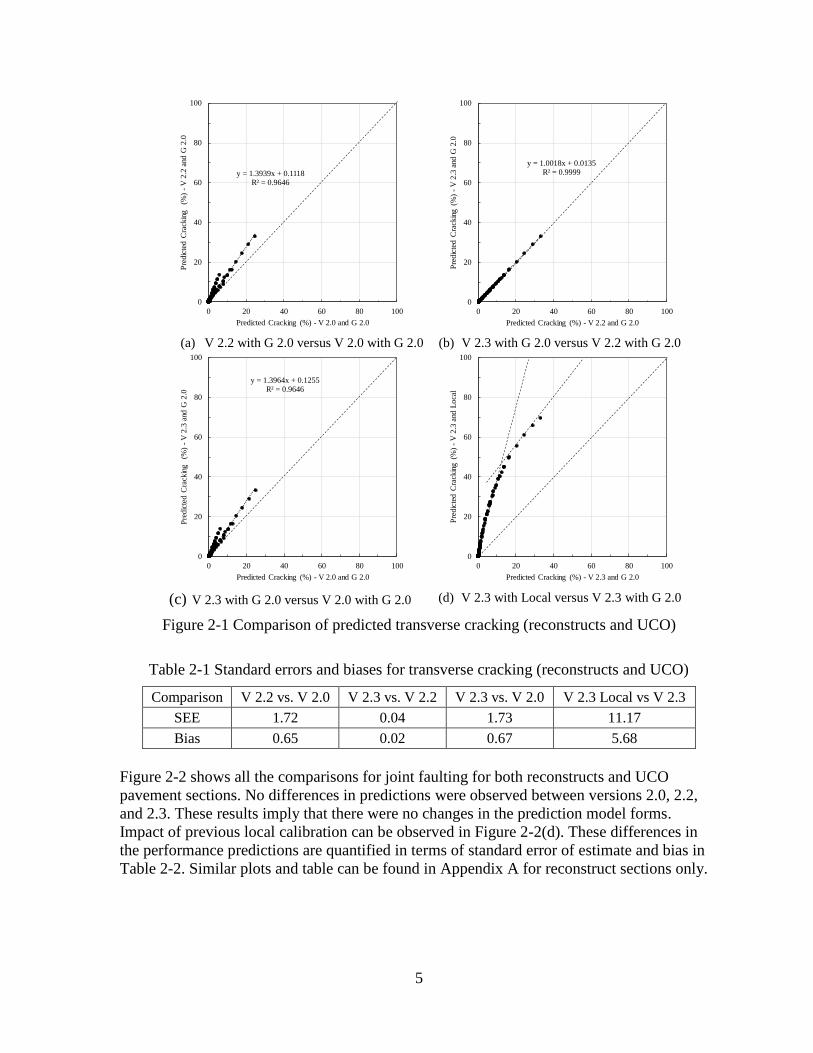
Three performance measures were compared for rigid pavements: (a) transverse cracking, (b)
faulting, and (c) pavement roughness in terms of International Roughness Index (IRI). Figure
2-1 shows all the above-mentioned comparisons for transverse cracking for both reconstructs
and unbonded concrete overlays (UCO) pavement sections. A total of 28 pavement sections
(20 reconstructs and 8 UCO) were used in these comparisons. It should be noted that the
same pavement sections were used for the previous local calibration. Some differences in
predictions were observed between versions 2.0 and 2.2, versions 2.0 and 2.3. However, no
difference in cracking predictions was observed between versions 2.2 and 2.3. These results
imply that there have been changes in the prediction model forms between versions 2.0 and
2.2. Impact of previous local calibration can be observed in Figure 2-1(d). These differences
in the performance predictions are quantified in terms of standard error of estimate and bias
in Table 2-1. Similar plots and table can be found in Appendix A for reconstruct sections
only.
5
(a) V 2.2 with G 2.0 versus V 2.0 with G 2.0
(b) V 2.3 with G 2.0 versus V 2.2 with G 2.0
(c) V 2.3 with G 2.0 versus V 2.0 with G 2.0
(d) V 2.3 with Local versus V 2.3 with G 2.0
Figure 2-1 Comparison of predicted transverse cracking (reconstructs and UCO)
Table 2-1 Standard errors and biases for transverse cracking (reconstructs and UCO)
Comparison V 2.2 vs. V 2.0 V 2.3 vs. V 2.2 V 2.3 vs. V 2.0 V 2.3 Local vs V 2.3
SEE 1.72 0.04 1.73 11.17
Bias 0.65 0.02 0.67 5.68
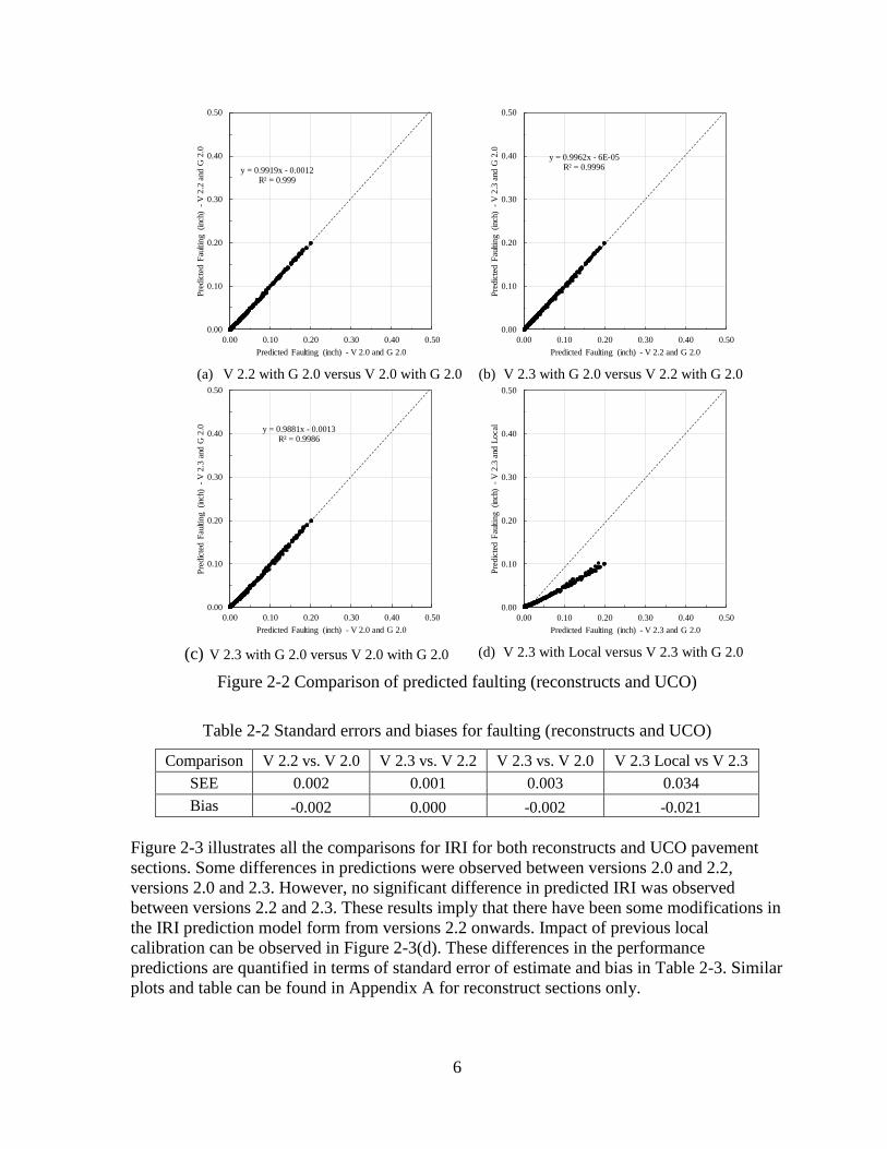
Figure 2-2 shows all the comparisons for joint faulting for both reconstructs and UCO
pavement sections. No differences in predictions were observed between versions 2.0, 2.2,
and 2.3. These results imply that there were no changes in the prediction model forms.
Impact of previous local calibration can be observed in Figure 2-2(d). These differences in
the performance predictions are quantified in terms of standard error of estimate and bias in
Table 2-2. Similar plots and table can be found in Appendix A for reconstruct sections only.
y = 1.3939x + 0.1118R² = 0.9646
0
20
40
60
80
100
0 20 40 60 80 100
Pre
dic
ted C
rack
ing
(%)
-V
2.2
and
G 2
.0
Predicted Cracking (%) - V 2.0 and G 2.0
y = 1.0018x + 0.0135R² = 0.9999
0
20
40
60
80
100
0 20 40 60 80 100
Pre
dic
ted C
rack
ing
(%)
-V
2.3
and
G 2
.0
Predicted Cracking (%) - V 2.2 and G 2.0
y = 1.3964x + 0.1255R² = 0.9646
0
20
40
60
80
100
0 20 40 60 80 100
Pre
dic
ted C
rack
ing
(%)
-V
2.3
and
G 2
.0
Predicted Cracking (%) - V 2.0 and G 2.0
0
20
40
60
80
100
0 20 40 60 80 100
Pre
dic
ted C
rack
ing
(%)
-V
2.3
and
Loca
l
Predicted Cracking (%) - V 2.3 and G 2.0
6
(a) V 2.2 with G 2.0 versus V 2.0 with G 2.0
(b) V 2.3 with G 2.0 versus V 2.2 with G 2.0
(c) V 2.3 with G 2.0 versus V 2.0 with G 2.0
(d) V 2.3 with Local versus V 2.3 with G 2.0
Figure 2-2 Comparison of predicted faulting (reconstructs and UCO)
Table 2-2 Standard errors and biases for faulting (reconstructs and UCO)
Comparison V 2.2 vs. V 2.0 V 2.3 vs. V 2.2 V 2.3 vs. V 2.0 V 2.3 Local vs V 2.3
SEE 0.002 0.001 0.003 0.034
Bias -0.002 0.000 -0.002 -0.021
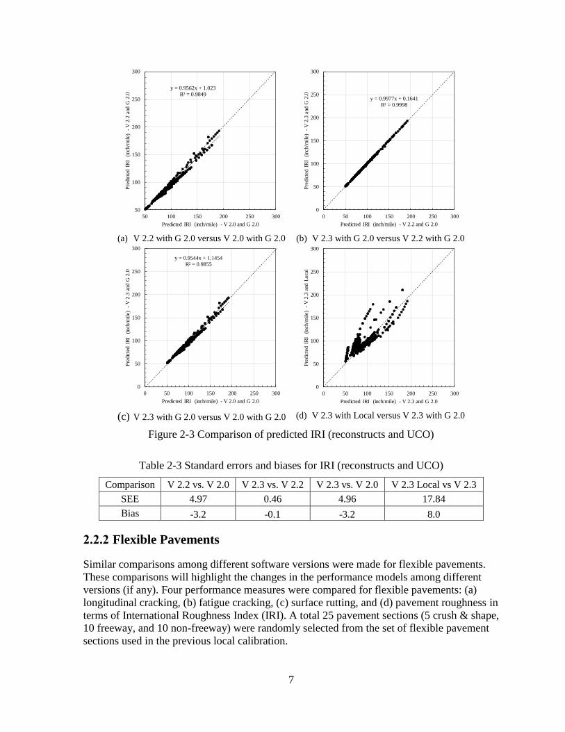
Figure 2-3 illustrates all the comparisons for IRI for both reconstructs and UCO pavement
sections. Some differences in predictions were observed between versions 2.0 and 2.2,
versions 2.0 and 2.3. However, no significant difference in predicted IRI was observed
between versions 2.2 and 2.3. These results imply that there have been some modifications in
the IRI prediction model form from versions 2.2 onwards. Impact of previous local
calibration can be observed in Figure 2-3(d). These differences in the performance
predictions are quantified in terms of standard error of estimate and bias in Table 2-3. Similar
plots and table can be found in Appendix A for reconstruct sections only.
y = 0.9919x - 0.0012R² = 0.999
0.00
0.10
0.20
0.30
0.40
0.50
0.00 0.10 0.20 0.30 0.40 0.50
Pre
dic
ted
Fau
ltin
g (inc
h)
-V
2.2
and
G 2
.0
Predicted Faulting (inch) - V 2.0 and G 2.0
y = 0.9962x - 6E-05R² = 0.9996
0.00
0.10
0.20
0.30
0.40
0.50
0.00 0.10 0.20 0.30 0.40 0.50
Pre
dic
ted
Fau
ltin
g (inc
h)
-V
2.3
and
G 2
.0
Predicted Faulting (inch) - V 2.2 and G 2.0
y = 0.9881x - 0.0013R² = 0.9986
0.00
0.10
0.20
0.30
0.40
0.50
0.00 0.10 0.20 0.30 0.40 0.50
Pre
dic
ted
Fau
ltin
g (inc
h)
-V
2.3
and
G 2
.0
Predicted Faulting (inch) - V 2.0 and G 2.0
0.00
0.10
0.20
0.30
0.40
0.50
0.00 0.10 0.20 0.30 0.40 0.50
Pre
dic
ted
Fau
ltin
g (inc
h)
-V
2.3
and
Lo
cal
Predicted Faulting (inch) - V 2.3 and G 2.0
7
(a) V 2.2 with G 2.0 versus V 2.0 with G 2.0
(b) V 2.3 with G 2.0 versus V 2.2 with G 2.0
(c) V 2.3 with G 2.0 versus V 2.0 with G 2.0
(d) V 2.3 with Local versus V 2.3 with G 2.0
Figure 2-3 Comparison of predicted IRI (reconstructs and UCO)
Table 2-3 Standard errors and biases for IRI (reconstructs and UCO)
Comparison V 2.2 vs. V 2.0 V 2.3 vs. V 2.2 V 2.3 vs. V 2.0 V 2.3 Local vs V 2.3
SEE 4.97 0.46 4.96 17.84
Bias -3.2 -0.1 -3.2 8.0
2.2.2 Flexible Pavements
Similar comparisons among different software versions were made for flexible pavements.
These comparisons will highlight the changes in the performance models among different
versions (if any). Four performance measures were compared for flexible pavements: (a)
longitudinal cracking, (b) fatigue cracking, (c) surface rutting, and (d) pavement roughness in
terms of International Roughness Index (IRI). A total 25 pavement sections (5 crush & shape,
10 freeway, and 10 non-freeway) were randomly selected from the set of flexible pavement
sections used in the previous local calibration.
y = 0.9562x + 1.023R² = 0.9849
50
100
150
200
250
300
50 100 150 200 250 300
Pre
dic
ted
IR
I (
inch
/mil
e)
-V
2.2
and
G 2
.0
Predicted IRI (inch/mile) - V 2.0 and G 2.0
y = 0.9977x + 0.1641R² = 0.9998
0
50
100
150
200
250
300
0 50 100 150 200 250 300
Pre
dic
ted
IR
I (
inch
/mile)
-
V 2
.3 a
nd G
2.0
Predicted IRI (inch/mile) - V 2.2 and G 2.0
y = 0.9544x + 1.1454R² = 0.9855
0
50
100
150
200
250
300
0 50 100 150 200 250 300
Pre
dic
ted
IR
I (
inch
/mile)
-
V 2
.3 a
nd G
2.0
Predicted IRI (inch/mile) - V 2.0 and G 2.0
0
50
100
150
200
250
300
0 50 100 150 200 250 300
Pre
dic
ted
IR
I (
inch
/mile)
-
V 2
.3 a
nd L
oca
l
Predicted IRI (inch/mile) - V 2.3 and G 2.0
8
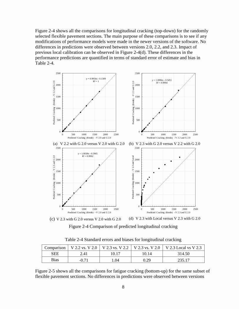
Figure 2-4 shows all the comparisons for longitudinal cracking (top-down) for the randomly
selected flexible pavement sections. The main purpose of these comparisons is to see if any
modifications of performance models were made in the newer versions of the software. No
differences in predictions were observed between versions 2.0, 2.2, and 2.3. Impact of
previous local calibration can be observed in Figure 2-4(d). These differences in the
performance predictions are quantified in terms of standard error of estimate and bias in
Table 2-4.
(a) V 2.2 with G 2.0 versus V 2.0 with G 2.0
(b) V 2.3 with G 2.0 versus V 2.2 with G 2.0
(c) V 2.3 with G 2.0 versus V 2.0 with G 2.0
(d) V 2.3 with Local versus V 2.3 with G 2.0
Figure 2-4 Comparison of predicted longitudinal cracking
Table 2-4 Standard errors and biases for longitudinal cracking
Comparison V 2.2 vs. V 2.0 V 2.3 vs. V 2.2 V 2.3 vs. V 2.0 V 2.3 Local vs V 2.3
SEE 2.41 10.17 10.14 314.50
Bias -0.71 1.04 0.29 235.17
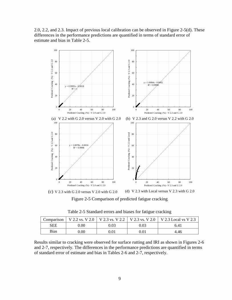
Figure 2-5 shows all the comparisons for fatigue cracking (bottom-up) for the same subset of
flexible pavement sections. No differences in predictions were observed between versions
y = 0.9956x - 0.1309R² = 1
0
500
1000
1500
2000
2500
0 500 1000 1500 2000 2500
Pre
dic
ted
Cra
ckin
g (f
t/m
ile)
-V
2.2
and
G 2
.0
Predicted Cracking (ft/mile) - V 2.0 and G 2.0
y = 1.0084x - 0.5451R² = 0.9994
0
500
1000
1500
2000
2500
0 500 1000 1500 2000 2500P
red
icte
d C
rack
ing
(ft/
mile
) -
V 2
.3 a
nd G
2.0
Predicted Cracking (ft/mile) - V 2.2 and G 2.0
y = 1.0038x - 0.5905R² = 0.9992
0
500
1000
1500
2000
2500
0 500 1000 1500 2000 2500
Pre
dic
ted
Cra
ckin
g (f
t/m
ile)
-V
2.3
and
G 2
.0
Predicted Cracking (ft/mile) - V 2.0 and G 2.0
0
500
1000
1500
2000
2500
0 500 1000 1500 2000 2500
Pre
dic
ted C
rack
ing
(ft/m
ile)
-V
2.3
and
Loca
l
Predicted Cracking (ft/mile) - V 2.3 and G 2.0
9
2.0, 2.2, and 2.3. Impact of previous local calibration can be observed in Figure 2-5(d). These
differences in the performance predictions are quantified in terms of standard error of
estimate and bias in Table 2-5.
(a) V 2.2 with G 2.0 versus V 2.0 with G 2.0
(b) V 2.3 and G 2.0 versus V 2.2 with G 2.0
(c) V 2.3 with G 2.0 versus V 2.0 with G 2.0
(d) V 2.3 with Local versus V 2.3 with G 2.0
Figure 2-5 Comparison of predicted fatigue cracking
Table 2-5 Standard errors and biases for fatigue cracking
Comparison V 2.2 vs. V 2.0 V 2.3 vs. V 2.2 V 2.3 vs. V 2.0 V 2.3 Local vs V 2.3
SEE 0.00 0.03 0.03 6.41
Bias 0.00 0.01 0.01 4.46
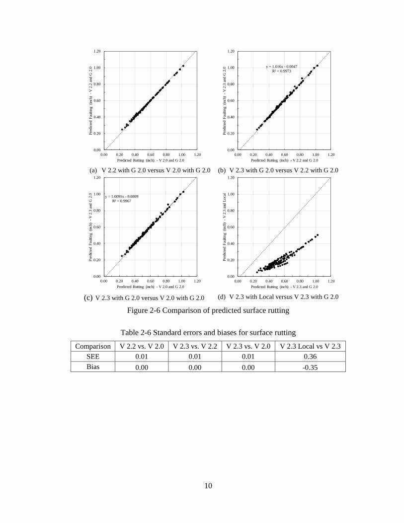
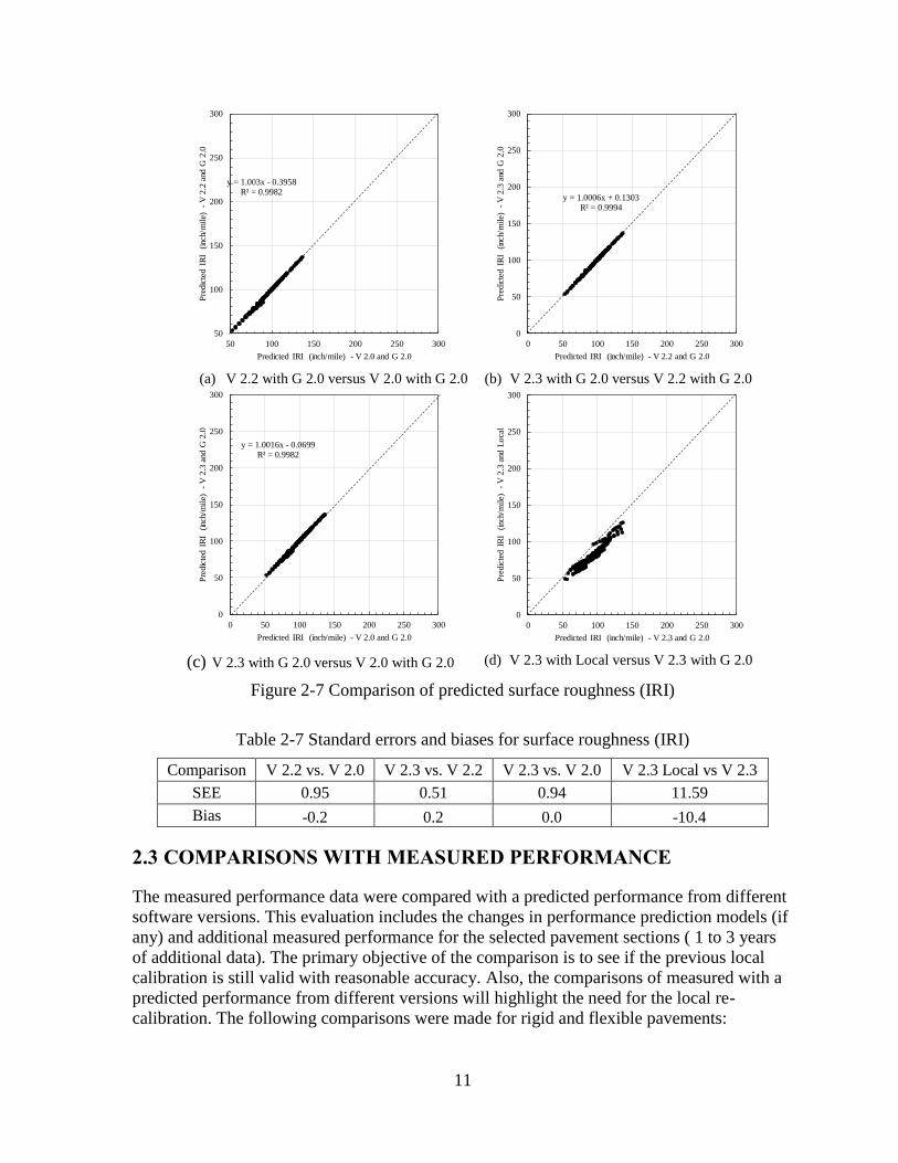
Results similar to cracking were observed for surface rutting and IRI as shown in Figures 2-6
and 2-7, respectively. The differences in the performance predictions are quantified in terms
of standard error of estimate and bias in Tables 2-6 and 2-7, respectively.
y = 0.9995x - 0.0018R² = 1
0
20
40
60
80
100
0 20 40 60 80 100
Pre
dic
ted
Cra
ckin
g (%
) -
V 2
.2 a
nd G
2.0
Predicted Cracking (%) - V 2.0 and G 2.0
y = 1.0084x - 0.0002R² = 0.9998
0
20
40
60
80
100
0 20 40 60 80 100
Pre
dic
ted
Cra
ckin
g(%
) -
V 2
.3 a
nd G
2.0
Predicted Cracking (%) - V 2.2 and G 2.0
y = 1.0078x - 0.0016R² = 0.9998
0
20
40
60
80
100
0 20 40 60 80 100
Pre
dic
ted
Cra
ckin
g (%
) -
V 2
.3 a
nd G
2.0
Predicted Cracking (%) - V 2.0 and G 2.0
0
20
40
60
80
100
0 20 40 60 80 100
Pre
dic
ted
Cra
ckin
g (%
)-
V 2
.3 a
nd L
oca
l
Predicted Cracking (%) - V 2.3 and G 2.0
10
(a) V 2.2 with G 2.0 versus V 2.0 with G 2.0
(b) V 2.3 with G 2.0 versus V 2.2 with G 2.0
(c) V 2.3 with G 2.0 versus V 2.0 with G 2.0
(d) V 2.3 with Local versus V 2.3 with G 2.0
Figure 2-6 Comparison of predicted surface rutting
Table 2-6 Standard errors and biases for surface rutting
Comparison V 2.2 vs. V 2.0 V 2.3 vs. V 2.2 V 2.3 vs. V 2.0 V 2.3 Local vs V 2.3
SEE 0.01 0.01 0.01 0.36
Bias 0.00 0.00 0.00 -0.35
0.00
0.20
0.40
0.60
0.80
1.00
1.20
0.00 0.20 0.40 0.60 0.80 1.00 1.20
Pre
dic
ted
Fau
ltin
g (inc
h)
-V
2.2
and
G 2
.0
Predicted Rutting (inch) - V 2.0 and G 2.0
y = 1.016x - 0.0047R² = 0.9973
0.00
0.20
0.40
0.60
0.80
1.00
1.20
0.00 0.20 0.40 0.60 0.80 1.00 1.20
Pre
dic
ted
Fau
ltin
g (inc
h)
-V
2.3
and
G 2
.0
Predicted Rutting (inch) - V 2.2 and G 2.0
y = 1.0095x - 0.0009R² = 0.9967
0.00
0.20
0.40
0.60
0.80
1.00
1.20
0.00 0.20 0.40 0.60 0.80 1.00 1.20
Pre
dic
ted
Fau
ltin
g (inc
h)
-V
2.3
and
G 2
.0
Predicted Rutting (inch) - V 2.0 and G 2.0
0.00
0.20
0.40
0.60
0.80
1.00
1.20
0.00 0.20 0.40 0.60 0.80 1.00 1.20
Pre
dic
ted
Fau
ltin
g (inc
h)
-V
2.3
and
Lo
cal
Predicted Rutting (inch) - V 2.3 and G 2.0
11
(a) V 2.2 with G 2.0 versus V 2.0 with G 2.0
(b) V 2.3 with G 2.0 versus V 2.2 with G 2.0
(c) V 2.3 with G 2.0 versus V 2.0 with G 2.0
(d) V 2.3 with Local versus V 2.3 with G 2.0
Figure 2-7 Comparison of predicted surface roughness (IRI)
Table 2-7 Standard errors and biases for surface roughness (IRI)
Comparison V 2.2 vs. V 2.0 V 2.3 vs. V 2.2 V 2.3 vs. V 2.0 V 2.3 Local vs V 2.3
SEE 0.95 0.51 0.94 11.59
Bias -0.2 0.2 0.0 -10.4
2.3 COMPARISONS WITH MEASURED PERFORMANCE
The measured performance data were compared with a predicted performance from different
software versions. This evaluation includes the changes in performance prediction models (if
any) and additional measured performance for the selected pavement sections ( 1 to 3 years
of additional data). The primary objective of the comparison is to see if the previous local
calibration is still valid with reasonable accuracy. Also, the comparisons of measured with a
predicted performance from different versions will highlight the need for the local re-
calibration. The following comparisons were made for rigid and flexible pavements:
y = 1.003x - 0.3958R² = 0.9982
50
100
150
200
250
300
50 100 150 200 250 300
Pre
dic
ted
IR
I (
inch
/mil
e)
-V
2.2
and
G 2
.0
Predicted IRI (inch/mile) - V 2.0 and G 2.0
y = 1.0006x + 0.1303R² = 0.9994
0
50
100
150
200
250
300
0 50 100 150 200 250 300
Pre
dic
ted
IR
I (
inch
/mile)
-
V 2
.3 a
nd G
2.0
Predicted IRI (inch/mile) - V 2.2 and G 2.0
y = 1.0016x - 0.0699R² = 0.9982
0
50
100
150
200
250
300
0 50 100 150 200 250 300
Pre
dic
ted
IR
I (
inch
/mile)
-
V 2
.3 a
nd G
2.0
Predicted IRI (inch/mile) - V 2.0 and G 2.0
0
50
100
150
200
250
300
0 50 100 150 200 250 300
Pre
dic
ted
IR
I (
inch
/mile)
-
V 2
.3 a
nd L
oca
l
Predicted IRI (inch/mile) - V 2.3 and G 2.0
12
1. Measured performance versus predicted performance by version 2.0 using version
2.0 global calibration coefficients (V 2.0 with G 2.0)
2. Measured performance versus V 2.2 with G 2.0
3. Measured performance versus V 2.3 with G 2.0
4. Measured performance versus V 2.3 with previous local calibration coefficients
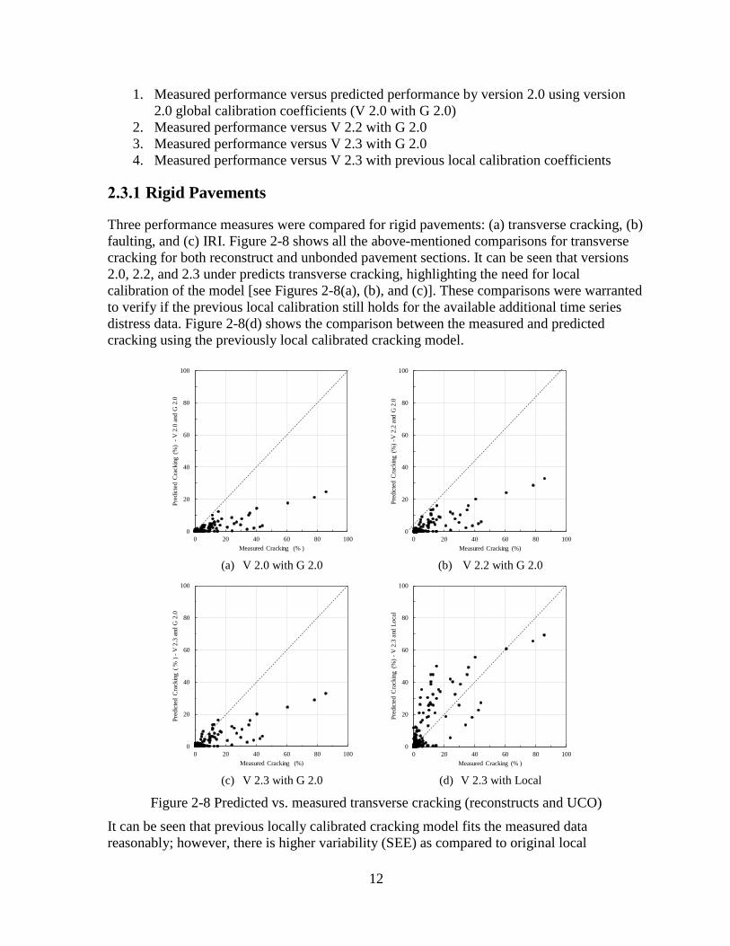
2.3.1 Rigid Pavements
Three performance measures were compared for rigid pavements: (a) transverse cracking, (b)
faulting, and (c) IRI. Figure 2-8 shows all the above-mentioned comparisons for transverse
cracking for both reconstruct and unbonded pavement sections. It can be seen that versions
2.0, 2.2, and 2.3 under predicts transverse cracking, highlighting the need for local
calibration of the model [see Figures 2-8(a), (b), and (c)]. These comparisons were warranted
to verify if the previous local calibration still holds for the available additional time series
distress data. Figure 2-8(d) shows the comparison between the measured and predicted
cracking using the previously local calibrated cracking model.
(a) V 2.0 with G 2.0
(b) V 2.2 with G 2.0
(c) V 2.3 with G 2.0
(d) V 2.3 with Local
Figure 2-8 Predicted vs. measured transverse cracking (reconstructs and UCO)
It can be seen that previous locally calibrated cracking model fits the measured data
reasonably; however, there is higher variability (SEE) as compared to original local
0
20
40
60
80
100
0 20 40 60 80 100
Pre
dic
ted
Cra
ckin
g (%
) -
V 2
.0 a
nd G
2.0
Measured Cracking (% )
0
20
40
60
80
100
0 20 40 60 80 100
Pre
dic
ted
Cra
ckin
g(%
) -V
2.2
and
G 2
.0
Measured Cracking (%)
0
20
40
60
80
100
0 20 40 60 80 100
Pre
dic
ted
Cra
ckin
g(
%)
-V
2.3
and
G 2
.0
Measured Cracking (%)
0
20
40
60
80
100
0 20 40 60 80 100
Pre
dic
ted
Cra
ckin
g(%
) -
V 2
.3 a
nd L
oca
l
Measured Cracking (% )
13
calibration (see Table 2-8). The causes of this variability could be attributed to modifications
in the model and additional measured cracking data (explained further in Chapter 3).
Table 2-8 Standard errors and biases between measured and predicted transverse cracking
(reconstructs and UCO)
Version V 2.0 V 2.2 V 2.3 V 2.3 Local
SEE 10.19 9.06 9.04 8.74
Bias -4.40 -3.75 -3.73 1.95
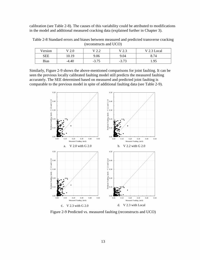
Similarly, Figure 2-9 shows the above-mentioned comparisons for joint faulting. It can be
seen the previous locally calibrated faulting model still predicts the measured faulting
accurately. The SEE determined based on measured and predicted joint faulting is
comparable to the previous model in spite of additional faulting data (see Table 2-9).
a. V 2.0 with G 2.0
b. V 2.2 with G 2.0
c. V 2.3 with G 2.0
d. V 2.3 with Local
Figure 2-9 Predicted vs. measured faulting (reconstructs and UCO)
0.00
0.10
0.20
0.30
0.40
0.50
0.00 0.10 0.20 0.30 0.40 0.50
Pre
dic
ted
Fau
ltin
g (i
nch)
-
V 2
.0 a
nd G
2.0
Measured Faulting (inch)
0.00
0.10
0.20
0.30
0.40
0.50
0.00 0.10 0.20 0.30 0.40 0.50
Pre
dic
ted
Fau
ltin
g (inc
h)
-V
2.2
and
G 2
.0
Measured Faulting (inch)
0.00
0.10
0.20
0.30
0.40
0.50
0.00 0.10 0.20 0.30 0.40 0.50
Pre
dic
ted
Fau
ltin
g (inc
h)
-V
2.3
and
G 2
.0
Measured Faulting (inch)
0.00
0.10
0.20
0.30
0.40
0.50
0.00 0.10 0.20 0.30 0.40 0.50
Pre
dic
ted
Fau
ltin
g (inc
h)
-V
2.3
and
Lo
cal
Measured Faulting (inch)
14
Table 2-9 Standard errors and biases between measured and predicted faulting (reconstructs and UCO)
Version V 2.0 V 2.2 V 2.3 V 2.3 Local
SEE 0.053 0.052 0.051 0.025
Bias 0.024 0.023 0.023 0.002
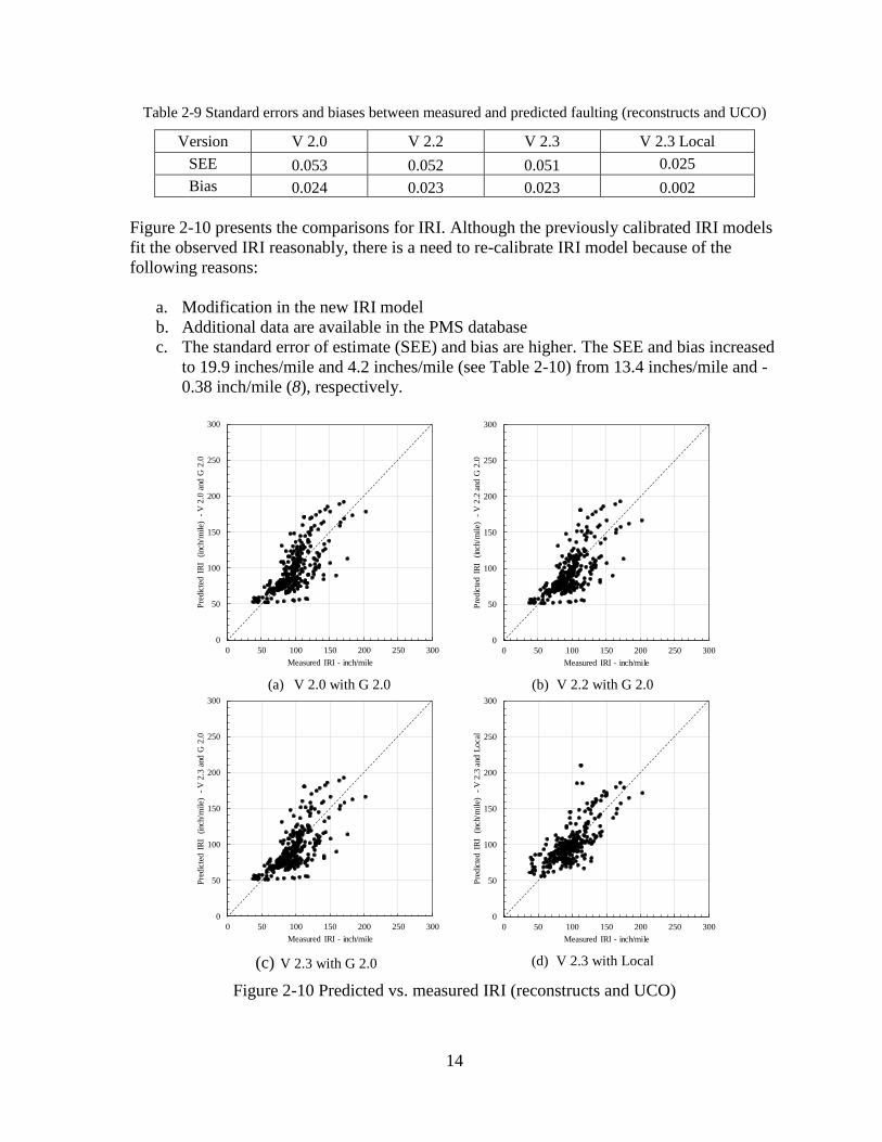
Figure 2-10 presents the comparisons for IRI. Although the previously calibrated IRI models
fit the observed IRI reasonably, there is a need to re-calibrate IRI model because of the
following reasons:
a. Modification in the new IRI model
b. Additional data are available in the PMS database
c. The standard error of estimate (SEE) and bias are higher. The SEE and bias increased
to 19.9 inches/mile and 4.2 inches/mile (see Table 2-10) from 13.4 inches/mile and -
0.38 inch/mile (8), respectively.
(a) V 2.0 with G 2.0
(b) V 2.2 with G 2.0
(c) V 2.3 with G 2.0
(d) V 2.3 with Local
Figure 2-10 Predicted vs. measured IRI (reconstructs and UCO)
0
50
100
150
200
250
300
0 50 100 150 200 250 300
Pre
dic
ted
IR
I (
inch
/mil
e)
-V
2.0
and
G 2
.0
Measured IRI - inch/mile
0
50
100
150
200
250
300
0 50 100 150 200 250 300
Pre
dic
ted
IR
I (
inch
/mile)
-
V 2
.2 a
nd G
2.0
Measured IRI - inch/mile
0
50
100
150
200
250
300
0 50 100 150 200 250 300
Pre
dic
ted
IR
I (
inch
/mile)
-
V 2
.3 a
nd G
2.0
Measured IRI - inch/mile
0
50
100
150
200
250
300
0 50 100 150 200 250 300
Pre
dic
ted
IR
I (
inch
/mile)
-
V 2
.3 a
nd L
oca
l
Measured IRI - inch/mile
15
Table 2-10 Standard errors and biases between measured and predicted IRI (reconstructs and UCO)
Version V 2.0 V 2.2 V 2.3 V 2.3 Local
SEE 20.9 21.1 21.1 19.9
Bias -0.6 -3.8 -3.8 4.2
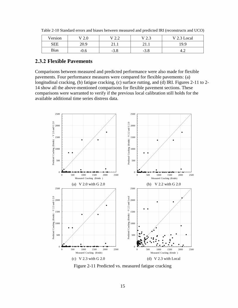
2.3.2 Flexible Pavements
Comparisons between measured and predicted performance were also made for flexible
pavements. Four performance measures were compared for flexible pavements: (a)
longitudinal cracking, (b) fatigue cracking, (c) surface rutting, and (d) IRI. Figures 2-11 to 2-
14 show all the above-mentioned comparisons for flexible pavement sections. These
comparisons were warranted to verify if the previous local calibration still holds for the
available additional time series distress data.
(a) V 2.0 with G 2.0
(b) V 2.2 with G 2.0
(c) V 2.3 with G 2.0
(d) V 2.3 with Local
Figure 2-11 Predicted vs. measured fatigue cracking
0
500
1000
1500
2000
2500
0 500 1000 1500 2000 2500
Pre
dic
ted C
rack
ing
(ft/m
ile)
-V
2.0
and
G 2
.0
Measured Cracking (ft/mile )
0
500
1000
1500
2000
2500
0 500 1000 1500 2000 2500
Pre
dic
ted C
rack
ing
(ft/
mile
) -V
2.2
and
G 2
.0
Measured Cracking (ft/mile)
0
500
1000
1500
2000
2500
0 500 1000 1500 2000 2500
Pre
dic
ted C
rack
ing
(ft/
mile
) -
V 2
.3 a
nd G
2.0
Measured Cracking (ft/mile)
0
500
1000
1500
2000
2500
0 500 1000 1500 2000 2500
Pre
dic
ted C
rack
ing
(ft/m
ile)
-V
2.3
and
Loca
l
Measured Cracking (ft/mile )

16
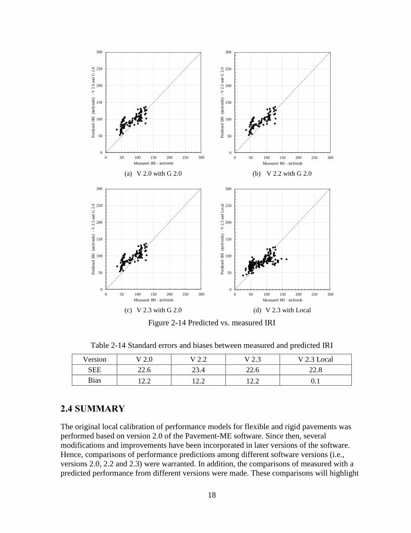
Tables 2-11 to 2-14 present SEE and bias for all the comparisons for flexible pavement
performance. For all the performance measures, the performance predictions show the
minimum SEE and bias using the previous locally calibrated coefficients in the models. It
should be noted that these comparisons were only made to verify the previous local
calibration efforts. This was accomplished by only using a subset of flexible pavement
sections from a larger set of the sections considered in previous calibration study. Therefore,
the current local calibration coefficient for flexible pavement models are still valid.
Table 2-11 Standard errors and biases between measured and predicted longitudinal cracking
Version V 2.0 V 2.2 V 2.3 V 2.3 Local
SEE 1213.53 1209.94 1212.40 1021.92
Bias -756.71 -747.22 -756.42 -441.21
(a) V 2.0 with G 2.0
(b) V 2.2 with G 2.0
(c) V 2.3 with G 2.0
(d) V 2.3 with Local
Figure 2-12 Predicted vs. measured fatigue cracking
0
20
40
60
80
100
0 20 40 60 80 100
Pre
dic
ted
Cra
ckin
g (%
) -
V 2
.0 a
nd G
2.0
Measured Cracking (% )
0
20
40
60
80
100
0 20 40 60 80 100
Pre
dic
ted
Cra
ckin
g(%
) -V
2.2
and
G 2
.0
Measured Cracking (%)
0
20
40
60
80
100
0 20 40 60 80 100
Pre
dic
ted
Cra
ckin
g(
%)
-V
2.3
and
G 2
.0
Measured Cracking (%)
0
20
40
60
80
100
0 20 40 60 80 100
Pre
dic
ted
Cra
ckin
g(%
) -
V 2
.3 a
nd L
oca
l
Measured Cracking (% )

17
Table 2-12 Standard errors and biases between measured and predicted fatigue cracking
Version V 2.0 V 2.2 V 2.3 V 2.3 Local
SEE 11.79 11.92 11.79 9.72
Bias -7.11 -7.14 -7.11 -2.12
(a) V 2.0 with G 2.0
(b) V 2.2 with G 2.0
(c) V 2.3 with G 2.0
(d) V 2.3 with Local
Figure 2-13 Predicted vs. measured rutting
Table 2-13 Standard errors and biases between measured and predicted rutting
Version V 2.0 V 2.2 V 2.3 V 2.3 Local
SEE 0.38 0.41 0.39 0.10
Bias 0.35 0.37 0.35 0.01
0.00
0.20
0.40
0.60
0.80
1.00
1.20
0.00 0.20 0.40 0.60 0.80 1.00 1.20
Pre
dic
ted
Rut
ting
(inc
h)
-V
2.0
and
G 2
.0
Measured Rutting (inch)
0.00
0.20
0.40
0.60
0.80
1.00
1.20
0.00 0.20 0.40 0.60 0.80 1.00 1.20P
red
icte
d R
uttin
g(inc
h)
-V
2.2
and
G 2
.0
Measured Rutting (inch)
0.00
0.20
0.40
0.60
0.80
1.00
1.20
0.00 0.20 0.40 0.60 0.80 1.00 1.20
Pre
dic
ted
Rut
ting
(inc
h)
-V
2.3
and
G 2
.0
Measured Rutting (inch)
0.00
0.20
0.40
0.60
0.80
1.00
1.20
0.00 0.20 0.40 0.60 0.80 1.00 1.20
Pre
dic
ted
Rut
ting
(inc
h)
-V
2.3
and
Lo
cal
Measured Rutting (inch)
18
(a) V 2.0 with G 2.0
(b) V 2.2 with G 2.0
(c) V 2.3 with G 2.0
(d) V 2.3 with Local
Figure 2-14 Predicted vs. measured IRI
Table 2-14 Standard errors and biases between measured and predicted IRI
Version V 2.0 V 2.2 V 2.3 V 2.3 Local
SEE 22.6 23.4 22.6 22.8
Bias 12.2 12.2 12.2 0.1
2.4 SUMMARY
The original local calibration of performance models for flexible and rigid pavements was
performed based on version 2.0 of the Pavement-ME software. Since then, several
modifications and improvements have been incorporated in later versions of the software.
Hence, comparisons of performance predictions among different software versions (i.e.,
versions 2.0, 2.2 and 2.3) were warranted. In addition, the comparisons of measured with a
predicted performance from different versions were made. These comparisons will highlight
0
50
100
150
200
250
300
0 50 100 150 200 250 300
Pre
dic
ted I
RI
(in
ch/m
ile)
-
V 2
.0 a
nd G
2.0
Measured IRI - inch/mile
0
50
100
150
200
250
300
0 50 100 150 200 250 300
Pre
dic
ted
IR
I (
inch
/mil
e)
-V
2.2
and
G 2
.0
Measured IRI - inch/mile
0
50
100
150
200
250
300
0 50 100 150 200 250 300
Pre
dic
ted
IR
I (
inch
/mile)
-
V 2
.3 a
nd G
2.0
Measured IRI - inch/mile
0
50
100
150
200
250
300
0 50 100 150 200 250 300
Pre
dic
ted I
RI
(in
ch/m
ile)
-
V 2
.3 a
nd L
oca
l
Measured IRI - inch/mile

19
the modifications in the models and the need for re-calibration. The results of the
comparisons show that performance models for rigid pavements (transverse cracking and
IRI) have changed since the Pavement-ME version 2.0. Because of these changes, and
additional time series data being available, re-calibration of the models is warranted. For
flexible pavement, the previous local calibration coefficients can still be used because the
prediction models are not modified since the Pavement-ME version 2.0.
20
CHAPTER 3 - RECALIBRATION OF RIGID PAVEMENT
PERFORMANCE MODELS
3.1 INTRODUCTION
The local calibration of the pavement performance prediction models is a challenging task
that requires a significant amount of preparation. The effectiveness of local calibration
depends on the input values and the measured pavement distress and roughness. Chapter 2
documented the need for re-calibration of rigid pavement performance models. This chapter
includes the results of the re-calibration of the performance prediction models using different
statistical techniques. The measured performance data from reconstruct and unbonded
overlays were used for recalibration. The performance prediction models were locally re-
calibrated by minimizing the sum of squared error between the measured and predicted
distresses by using the following statistical sampling techniques:
a. No sampling (include all data)
b. Bootstrapping
c. Repeated split sampling
The different sampling techniques (a to c) were used to determine the best estimate of the
local calibration coefficients and the associated standard errors. The use of these techniques
is considered because of data limitations, especially due to limited sample size for rigid
pavements, and to utilize a more robust way of quantifying model standard error and bias.
The following rigid pavement performance models in the Pavement-ME were locally re-
calibrated for Michigan conditions.
Transverse cracking
Faulting
IRI
The Pavement-ME software version 2.3 was executed using the as-constructed inputs for all
the selected pavement sections and the predicted performance was extracted from the output
files. The measured and predicted distresses over time were compared. These comparisons
evaluate the adequacy of global model predictions for the measured distresses on the
pavement sections. Generally, the predicted and measured performance should have a one-to-
one (45-degree line of equality) relationship in the case of a good match. Otherwise, biased
and/or prediction error may exist based on the spread of data around the line of equality. As a
consequence, local calibration of the model is needed to reduce the bias and standard error
between the predicted and measured performance.
21
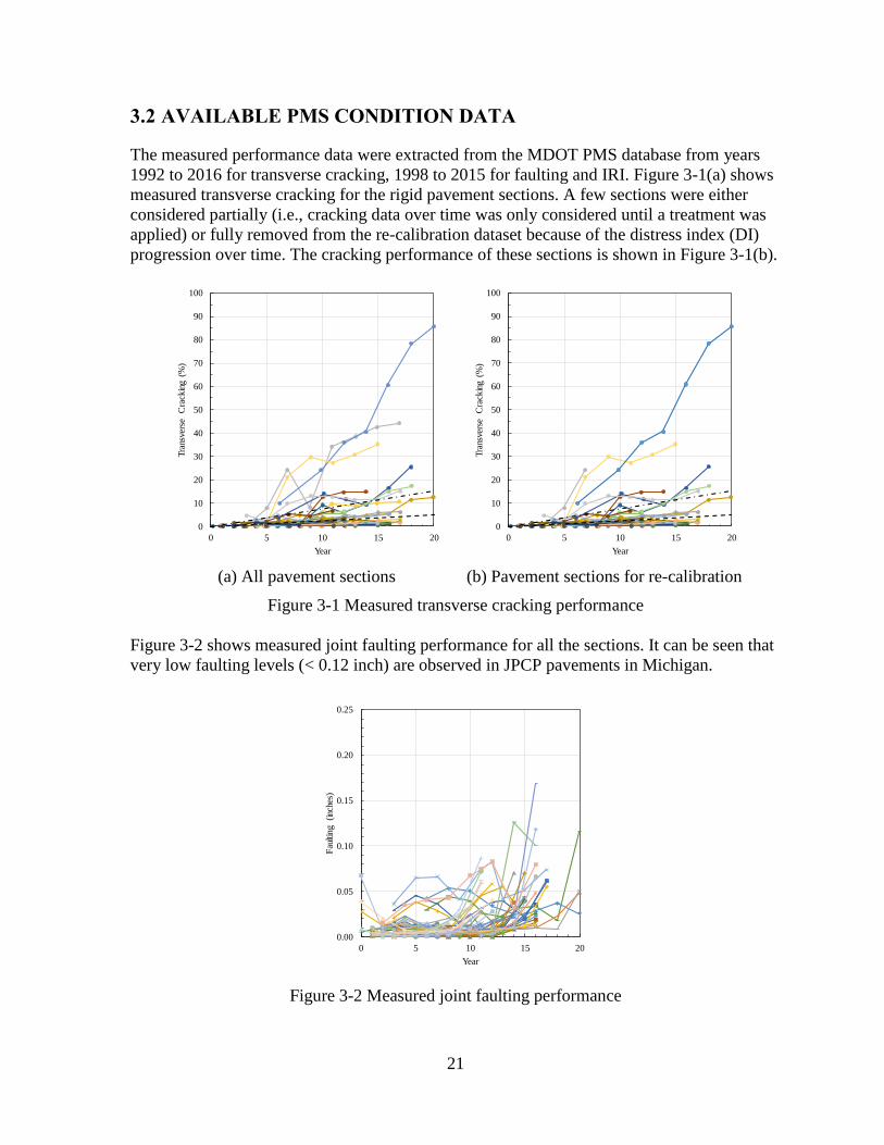
3.2 AVAILABLE PMS CONDITION DATA
The measured performance data were extracted from the MDOT PMS database from years
1992 to 2016 for transverse cracking, 1998 to 2015 for faulting and IRI. Figure 3-1(a) shows
measured transverse cracking for the rigid pavement sections. A few sections were either
considered partially (i.e., cracking data over time was only considered until a treatment was
applied) or fully removed from the re-calibration dataset because of the distress index (DI)
progression over time. The cracking performance of these sections is shown in Figure 3-1(b).
(a) All pavement sections
(b) Pavement sections for re-calibration
Figure 3-1 Measured transverse cracking performance
Figure 3-2 shows measured joint faulting performance for all the sections. It can be seen that
very low faulting levels (< 0.12 inch) are observed in JPCP pavements in Michigan.
Figure 3-2 Measured joint faulting performance
0
10
20
30
40
50
60
70
80
90
100
0 5 10 15 20
Tra
nsve
rse
Cra
ckin
g (%
)
Year
0
10
20
30
40
50
60
70
80
90
100
0 5 10 15 20
Tra
nsve
rse
Cra
ckin
g (%
)
Year
0.00
0.05
0.10
0.15
0.20
0.25
0 5 10 15 20
Fau
lting
(inc
hes)
Year
22
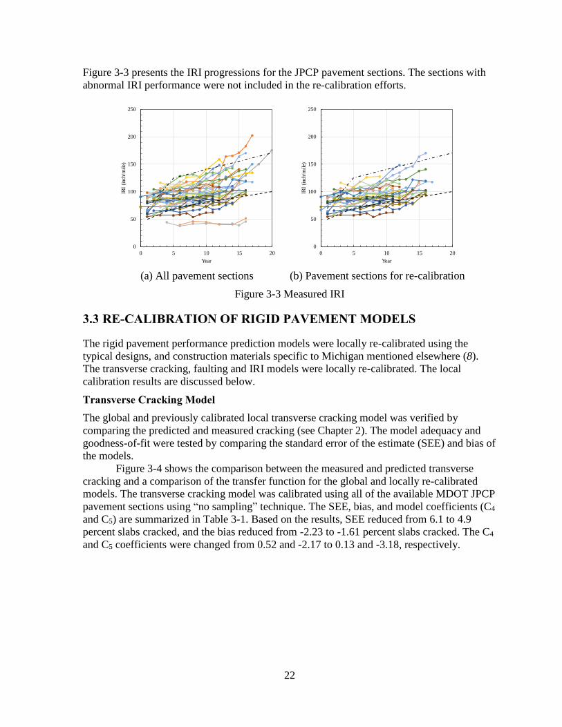
Figure 3-3 presents the IRI progressions for the JPCP pavement sections. The sections with
abnormal IRI performance were not included in the re-calibration efforts.
(a) All pavement sections
(b) Pavement sections for re-calibration
Figure 3-3 Measured IRI
3.3 RE-CALIBRATION OF RIGID PAVEMENT MODELS
The rigid pavement performance prediction models were locally re-calibrated using the
typical designs, and construction materials specific to Michigan mentioned elsewhere (8).
The transverse cracking, faulting and IRI models were locally re-calibrated. The local
calibration results are discussed below.
Transverse Cracking Model
The global and previously calibrated local transverse cracking model was verified by
comparing the predicted and measured cracking (see Chapter 2). The model adequacy and
goodness-of-fit were tested by comparing the standard error of the estimate (SEE) and bias of
the models.
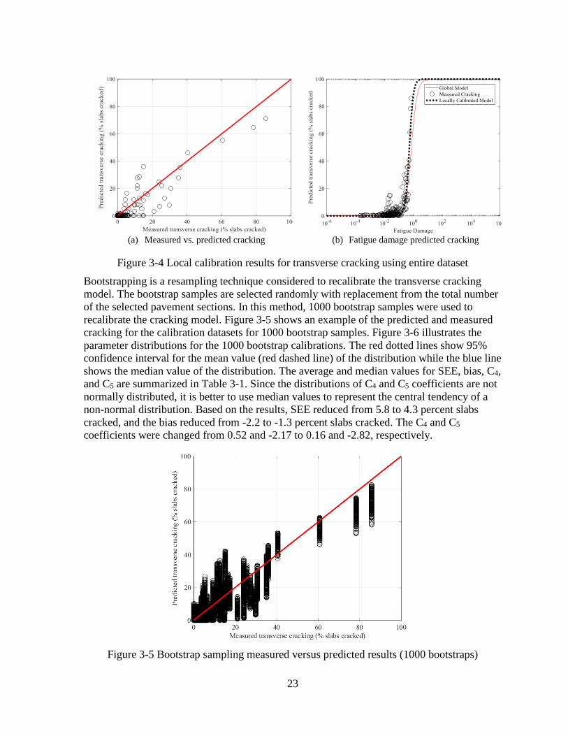
Figure 3-4 shows the comparison between the measured and predicted transverse
cracking and a comparison of the transfer function for the global and locally re-calibrated
models. The transverse cracking model was calibrated using all of the available MDOT JPCP
pavement sections using “no sampling” technique. The SEE, bias, and model coefficients (C4
and C5) are summarized in Table 3-1. Based on the results, SEE reduced from 6.1 to 4.9
percent slabs cracked, and the bias reduced from -2.23 to -1.61 percent slabs cracked. The C4
and C5 coefficients were changed from 0.52 and -2.17 to 0.13 and -3.18, respectively.
0
50
100
150
200
250
0 5 10 15 20
IRI
(inc
h/m
ile)
Year
0
50
100
150
200
250
0 5 10 15 20
IRI
(inc
h/m
ile)
Year
23
(a) Measured vs. predicted cracking
(b) Fatigue damage predicted cracking
Figure 3-4 Local calibration results for transverse cracking using entire dataset
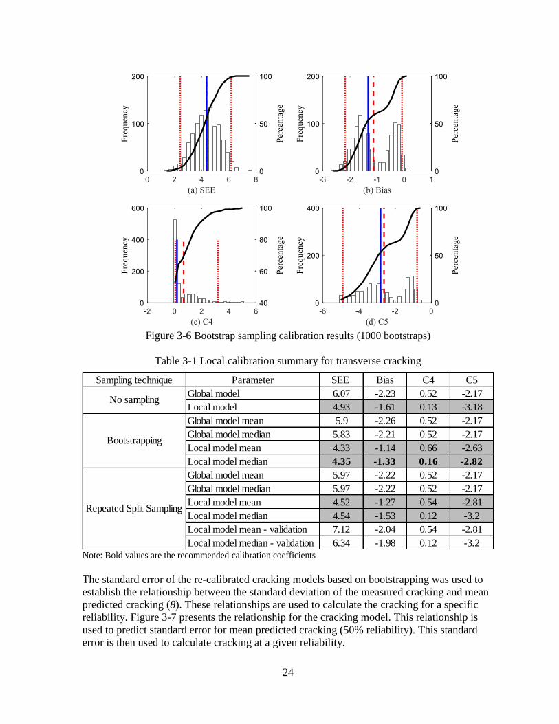
Bootstrapping is a resampling technique considered to recalibrate the transverse cracking
model. The bootstrap samples are selected randomly with replacement from the total number
of the selected pavement sections. In this method, 1000 bootstrap samples were used to
recalibrate the cracking model. Figure 3-5 shows an example of the predicted and measured
cracking for the calibration datasets for 1000 bootstrap samples. Figure 3-6 illustrates the
parameter distributions for the 1000 bootstrap calibrations. The red dotted lines show 95%
confidence interval for the mean value (red dashed line) of the distribution while the blue line
shows the median value of the distribution. The average and median values for SEE, bias, C4,
and C5 are summarized in Table 3-1. Since the distributions of C4 and C5 coefficients are not
normally distributed, it is better to use median values to represent the central tendency of a
non-normal distribution. Based on the results, SEE reduced from 5.8 to 4.3 percent slabs
cracked, and the bias reduced from -2.2 to -1.3 percent slabs cracked. The C4 and C5
coefficients were changed from 0.52 and -2.17 to 0.16 and -2.82, respectively.
Figure 3-5 Bootstrap sampling measured versus predicted results (1000 bootstraps)
24
Figure 3-6 Bootstrap sampling calibration results (1000 bootstraps)
Table 3-1 Local calibration summary for transverse cracking
Note: Bold values are the recommended calibration coefficients
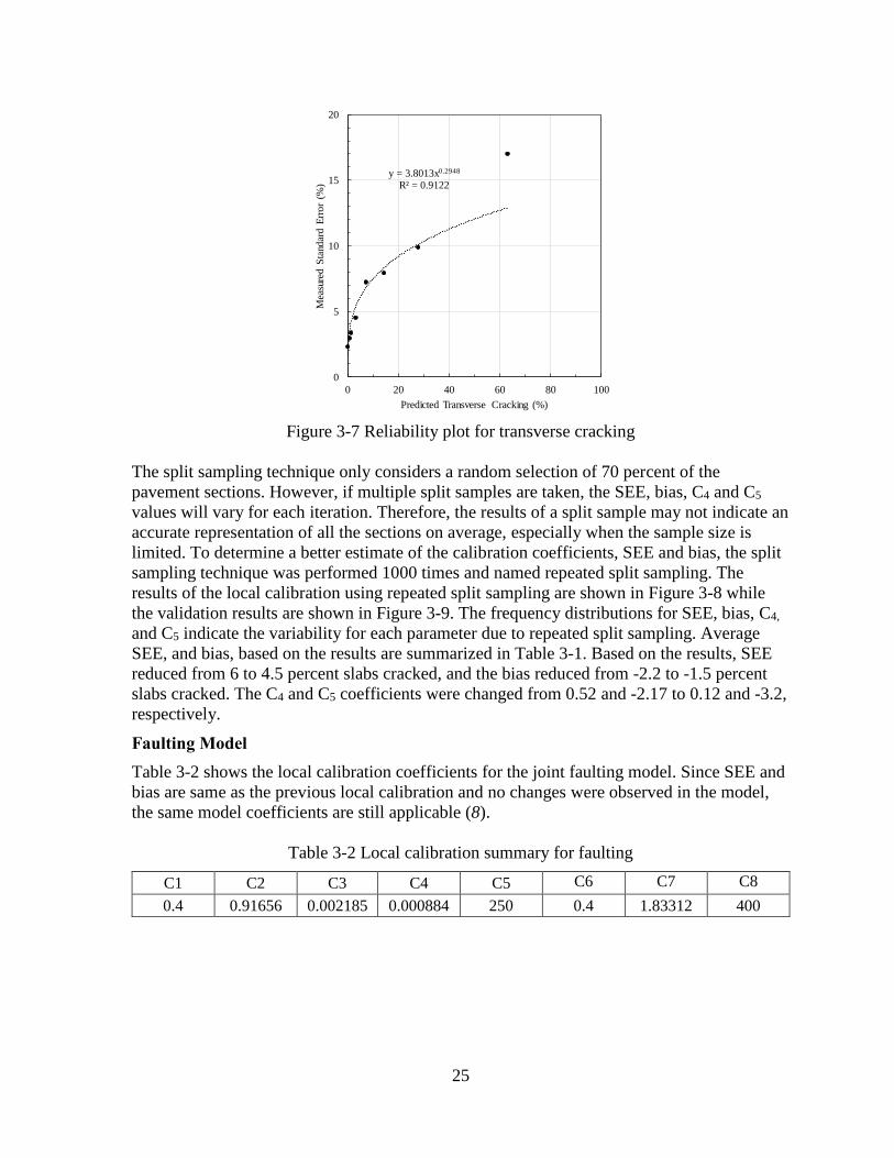
The standard error of the re-calibrated cracking models based on bootstrapping was used to
establish the relationship between the standard deviation of the measured cracking and mean
predicted cracking (8). These relationships are used to calculate the cracking for a specific
reliability. Figure 3-7 presents the relationship for the cracking model. This relationship is
used to predict standard error for mean predicted cracking (50% reliability). This standard
error is then used to calculate cracking at a given reliability.
Sampling technique Parameter SEE Bias C4 C5
Global model 6.07 -2.23 0.52 -2.17
Local model 4.93 -1.61 0.13 -3.18
Global model mean 5.9 -2.26 0.52 -2.17
Global model median 5.83 -2.21 0.52 -2.17
Local model mean 4.33 -1.14 0.66 -2.63
Local model median 4.35 -1.33 0.16 -2.82
Global model mean 5.97 -2.22 0.52 -2.17
Global model median 5.97 -2.22 0.52 -2.17
Local model mean 4.52 -1.27 0.54 -2.81
Local model median 4.54 -1.53 0.12 -3.2
Local model mean - validation 7.12 -2.04 0.54 -2.81
Local model median - validation 6.34 -1.98 0.12 -3.2
No sampling
Bootstrapping
Repeated Split Sampling
25
Figure 3-7 Reliability plot for transverse cracking
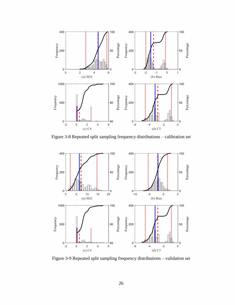
The split sampling technique only considers a random selection of 70 percent of the
pavement sections. However, if multiple split samples are taken, the SEE, bias, C4 and C5
values will vary for each iteration. Therefore, the results of a split sample may not indicate an
accurate representation of all the sections on average, especially when the sample size is
limited. To determine a better estimate of the calibration coefficients, SEE and bias, the split
sampling technique was performed 1000 times and named repeated split sampling. The
results of the local calibration using repeated split sampling are shown in Figure 3-8 while
the validation results are shown in Figure 3-9. The frequency distributions for SEE, bias, C4,
and C5 indicate the variability for each parameter due to repeated split sampling. Average
SEE, and bias, based on the results are summarized in Table 3-1. Based on the results, SEE
reduced from 6 to 4.5 percent slabs cracked, and the bias reduced from -2.2 to -1.5 percent
slabs cracked. The C4 and C5 coefficients were changed from 0.52 and -2.17 to 0.12 and -3.2,
respectively.
Faulting Model
Table 3-2 shows the local calibration coefficients for the joint faulting model. Since SEE and
bias are same as the previous local calibration and no changes were observed in the model,
the same model coefficients are still applicable (8).
Table 3-2 Local calibration summary for faulting
C1 C2 C3 C4 C5 C6 C7 C8
0.4 0.91656 0.002185 0.000884 250 0.4 1.83312 400
y = 3.8013x0.2948
R² = 0.9122
0
5
10
15
20
0 20 40 60 80 100
Mea
sure
d S
tand
ard E
rror
(%)
Predicted Transverse Cracking (%)
26
Figure 3-8 Repeated split sampling frequency distributions – calibration set
Figure 3-9 Repeated split sampling frequency distributions – validation set
27
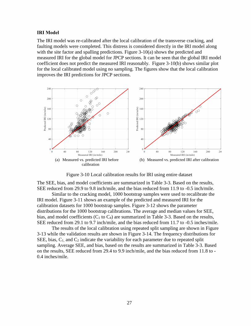
IRI Model
The IRI model was re-calibrated after the local calibration of the transverse cracking, and
faulting models were completed. This distress is considered directly in the IRI model along
with the site factor and spalling predictions. Figure 3-10(a) shows the predicted and
measured IRI for the global model for JPCP sections. It can be seen that the global IRI model
coefficient does not predict the measured IRI reasonably. Figure 3-10(b) shows similar plot
for the local calibrated model using no sampling. The figures show that the local calibration
improves the IRI predictions for JPCP sections.
(a) Measured vs. predicted IRI before
calibration
(b) Measured vs. predicted IRI after calibration
Figure 3-10 Local calibration results for IRI using entire dataset
The SEE, bias, and model coefficients are summarized in Table 3-3. Based on the results,
SEE reduced from 29.9 to 9.8 inch/mile, and the bias reduced from 11.9 to -0.5 inch/mile.
Similar to the cracking model, 1000 bootstrap samples were used to recalibrate the
IRI model. Figure 3-11 shows an example of the predicted and measured IRI for the
calibration datasets for 1000 bootstrap samples. Figure 3-12 shows the parameter
distributions for the 1000 bootstrap calibrations. The average and median values for SEE,
bias, and model coefficients (C1 to C4) are summarized in Table 3-3. Based on the results,
SEE reduced from 29.1 to 9.7 inch/mile, and the bias reduced from 11.7 to -0.5 inches/mile.
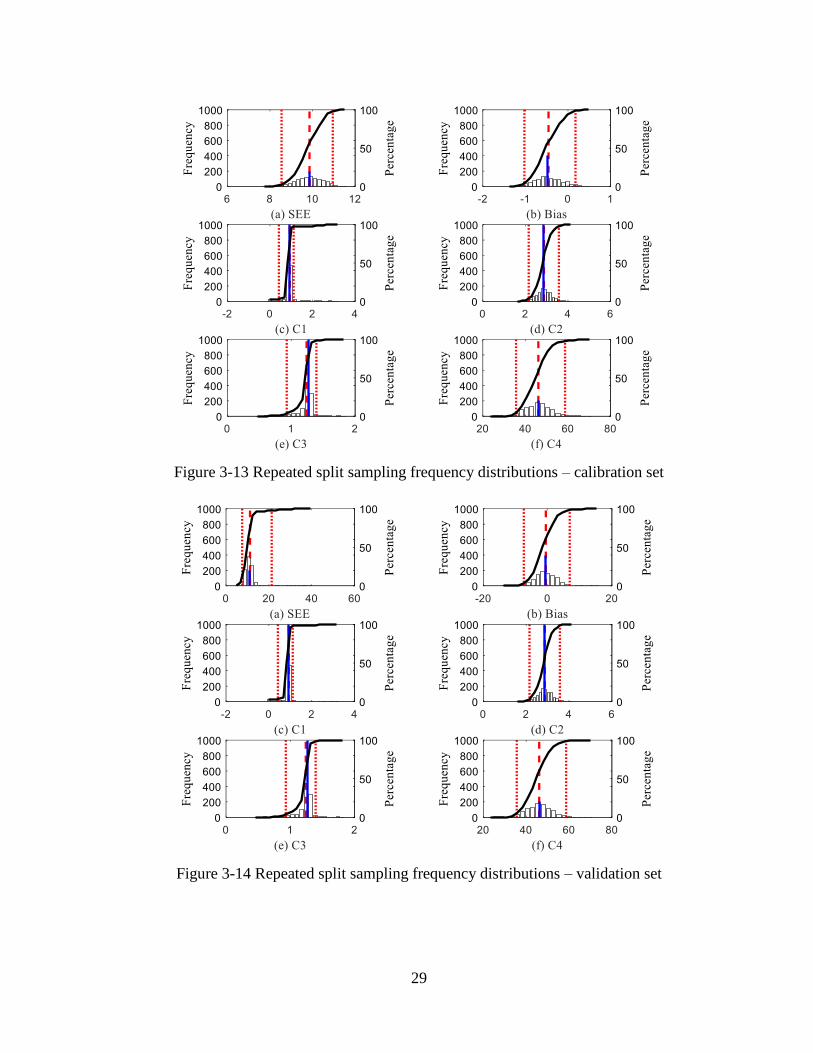
The results of the local calibration using repeated split sampling are shown in Figure
3-13 while the validation results are shown in Figure 3-14. The frequency distributions for
SEE, bias, C1, and C2 indicate the variability for each parameter due to repeated split
sampling. Average SEE, and bias, based on the results are summarized in Table 3-3. Based
on the results, SEE reduced from 29.4 to 9.9 inch/mile, and the bias reduced from 11.8 to -
0.4 inches/mile.

28
Figure 3-11 Bootstrap sampling measured versus predicted results (1000 bootstraps)
Figure 3-12 Bootstrap sampling calibration results (1000 bootstraps)
29
Figure 3-13 Repeated split sampling frequency distributions – calibration set
Figure 3-14 Repeated split sampling frequency distributions – validation set

30
Table 3-3 Local calibration summary for IRI
Note: Bold values are the recommended calibration coefficients
3.4 IMPLEMENTATION CHALLENGES
After the re-calibration of cracking and IRI models, several previously ME designed
pavement projects were redesigned using the revised coefficients. These design evaluations
highlighted potential issues in implementing the Pavement-ME for rigid pavements in
Michigan as discussed below.
3.4.1 Impact of Re-calibration on Pavement Designs
The initial design thicknesses are based on AASHTO 93. For the same design, different
Pavement-ME versions were used to analyze the thickness for which the predicted pavement
performance is 15% slabs cracked or 172 inches/mile for transverse cracking and IRI,
respectively at 20 years. Another criteria used by MDOT is to limit the designed slab
thickness by the Pavement-ME within ±1 inch of AASHTO 93 design thickness. That means
even if the designed slab thickness lesser than 1 inch as compared to AASHTO 93, it will be
restricted to 1 inch thinner than the initial design and vice versa. For example, if the designed
slab thickness is 9 inches and initial AASHTO design thickness corresponds to 10.5 inches,
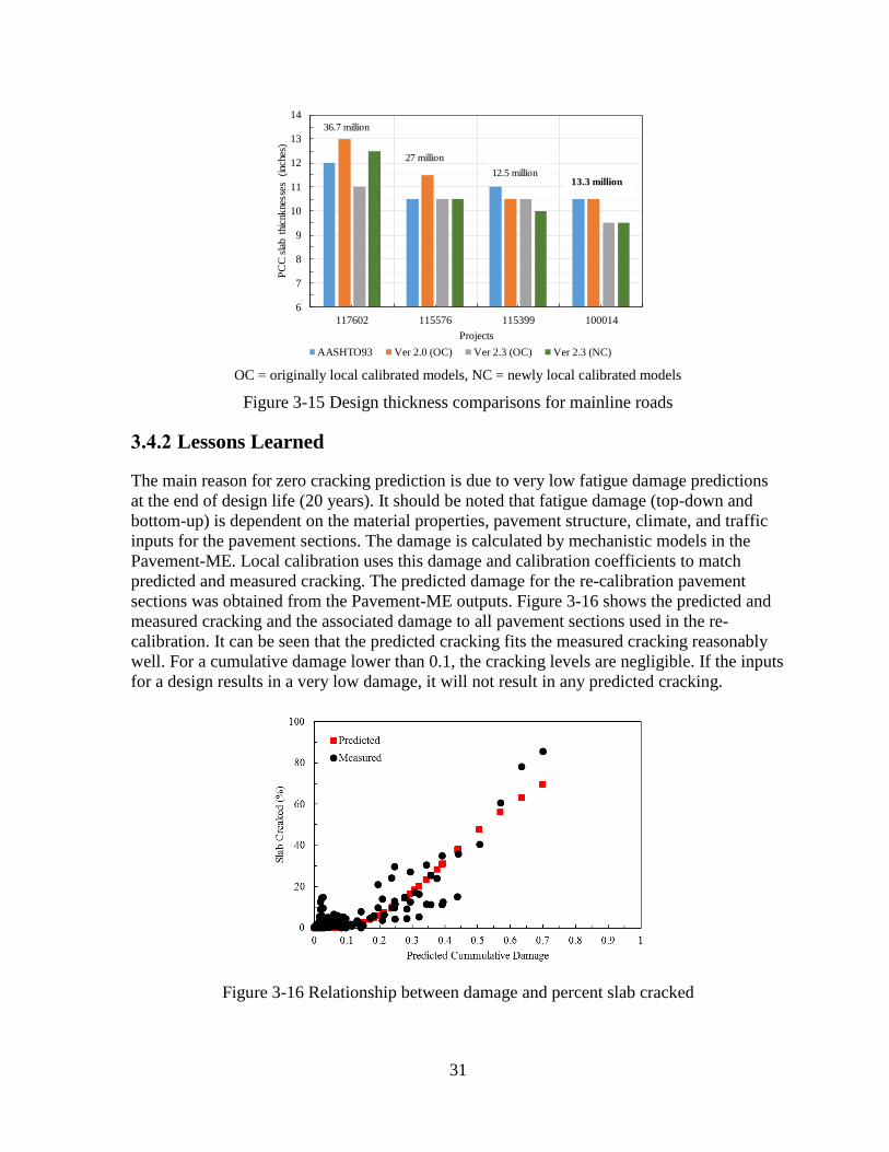
the final slab thickness will be 9.5 inches. Figure 3-15 shows the comparison of PCC slab
thicknesses designed by using AASHTO 93, the Pavement-ME versions 2.0 and 2.3 using
previous local calibration coefficients, and the version 2.3 using re-calibrated coefficients for
four mainline pavement designs. The critical distress for all the designs was IRI, and all
designs showed no predicted cracking. However, noticeable cracking was observed in a few
pavement sections used for re-calibration. MDOT engineers were concerned with the no
cracking prediction by the Pavement-ME. The probable causes for no cracking prediction
were investigated, and the findings are discussed in the next section.
Sampling technique Parameter SEE Bias C1 C2 C3 C4
Global model 29.89 11.92 0.82 0.44 1.49 25.24
Local model 9.83 -0.54 2.23 2.87 1.33 43.89
Global model mean 29.09 11.74 0.82 0.44 1.49 25.24
Global model median 28.82 11.52 0.82 0.44 1.49 25.24
Local model mean 9.72 -0.47 0.95 2.9 1.21 47.06
Local model median 9.72 -0.45 0.91 2.9 1.26 45.82
Global model mean 29.44 11.76 0.82 0.44 1.49 25.24
Global model median 31.44 12.16 0.82 0.44 1.49 25.24
Local model mean 9.86 -0.44 0.93 2.89 1.23 46.39
Local model median 9.92 -0.46 0.91 2.89 1.26 46.21
Local model mean - validation 11.3 -0.47 0.93 2.89 1.23 46.39
Local model median - validation 10.71 -0.64 0.91 2.89 1.26 46.21
No sampling
Bootstrapping
Repeated Split Sampling
31
OC = originally local calibrated models, NC = newly local calibrated models
Figure 3-15 Design thickness comparisons for mainline roads
3.4.2 Lessons Learned
The main reason for zero cracking prediction is due to very low fatigue damage predictions
at the end of design life (20 years). It should be noted that fatigue damage (top-down and
bottom-up) is dependent on the material properties, pavement structure, climate, and traffic
inputs for the pavement sections. The damage is calculated by mechanistic models in the
Pavement-ME. Local calibration uses this damage and calibration coefficients to match
predicted and measured cracking. The predicted damage for the re-calibration pavement
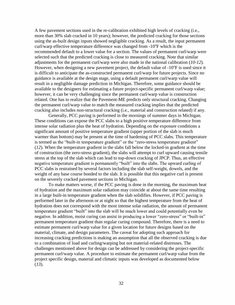
sections was obtained from the Pavement-ME outputs. Figure 3-16 shows the predicted and
measured cracking and the associated damage to all pavement sections used in the re-
calibration. It can be seen that the predicted cracking fits the measured cracking reasonably
well. For a cumulative damage lower than 0.1, the cracking levels are negligible. If the inputs
for a design results in a very low damage, it will not result in any predicted cracking.
Figure 3-16 Relationship between damage and percent slab cracked
6
7
8
9
10
11
12
13
14
117602 115576 115399 100014
PC
C s
lab t
hicn
kne
sses
(inc
hes)
Projects
AASHTO93 Ver 2.0 (OC) Ver 2.3 (OC) Ver 2.3 (NC)
27 million
12.5 million13.3 million
36.7 million
32
A few pavement sections used in the re-calibration exhibited high levels of cracking (i.e.,
more than 30% slab cracked in 10 years); however, the predicted cracking for those sections
using the as-built design inputs showed negligible cracking. As a result, the input permanent
curl/warp effective temperature difference was changed from -10oF which is the
recommended default to a lower value for a section. The values of permanent curl/warp were
selected such that the predicted cracking is close to measured cracking. Note that similar
adjustments for the permanent curl/warp were also made in the national calibration (10-12).
However, when designing a new pavement project, the default value of -10oF is used since it
is difficult to anticipate the as-constructed permanent curl/warp for future projects. Since no
guidance is available at the design stage, using a default permanent curl/warp value will
result in a negligible damage prediction in Michigan. Therefore, some guidance should be
available to the designers for estimating a future project-specific permanent curl/warp value;
however, it can be very challenging since the permanent curl/warp value is construction
related. One has to realize that the Pavement-ME predicts only structural cracking. Changing
the permanent curl/warp value to match the measured cracking implies that the predicted
cracking also includes non-structural cracking (i.e., material and construction related) if any.
Generally, PCC paving is performed in the mornings of summer days in Michigan.
These conditions can expose the PCC slabs to a high positive temperature difference from
intense solar radiation plus the heat of hydration. Depending on the exposure conditions a
significant amount of positive temperature gradient (upper portion of the slab is much
warmer than bottom) may be present at the time of hardening of PCC slabs. This temperature
is termed as the “built-in temperature gradient” or the “zero-stress temperature gradient”
(12). When the temperature gradient in the slabs fall below the locked-in gradient at the time
of construction (the zero-stress gradient), the slabs will attempt to curl upward causing tensile
stress at the top of the slab which can lead to top-down cracking of JPCP. Thus, an effective
negative temperature gradient is permanently “built” into the slabs. The upward curling of
PCC slabs is restrained by several factors including the slab self-weight, dowels, and the
weight of any base course bonded to the slab. It is possible that this negative curl is present
on the severely cracked pavement sections in Michigan.
To make matters worse, if the PCC paving is done in the morning, the maximum heat
of hydration and the maximum solar radiation may coincide at about the same time resulting
in a large built-in temperature gradient when the slab solidifies. However, if PCC paving is
performed later in the afternoon or at night so that the highest temperature from the heat of
hydration does not correspond with the most intense solar radiation, the amount of permanent
temperature gradient “built” into the slab will be much lower and could potentially even be
negative. In addition, moist curing can assist in producing a lower “zero-stress” or “built-in”
permanent temperature gradient than regular curing compound. Therefore, there is a need to
estimate permanent curl/warp value for a given location for future designs based on the
material, climate, and design parameters. The caveat for adopting such approach for
increasing cracking predictions is making an assumption that all the observed cracking is due
to a combination of load and curling/warping but not material-related distresses. The
challenges mentioned above for design can be addressed by considering the project-specific
permanent curl/warp value. A procedure to estimate the permanent curl/warp value from the
project specific design, material and climatic inputs was developed as documented below
(13).
33
3.5 PERMANENT CURL/WARP MODEL
The permanent curl/warp of a pavement section depends on its material, climate and design
parameters. Several inputs related to material properties (i.e., compressive strength,
aggregate type, etc.), design parameters (slab thickness, slab width, joint spacing, etc.), and
climatic data (wind speed, temperatures, and precipitation related, etc.) were obtained for
each of the pavement sections used in re-calibration. For each section, the permanent curl
values were estimated by matching measured and predicted cracking (version 2.3 global
coefficients). These estimated permanent curl values were used as dependent variable, and
all other inputs mentioned above were used as impendent variables. Several models were
fitted to explain the relationship between the site-specific permanent curl and the inputs.
Based on the goodness-of-fit ( 2 0.918R ) and practical impact of the variables on the curl,
the following model was chosen to predict permanent curl per inch. The predicted permanent
curl is a function of compressive strength, average wind speed, mean annual precipitation,
and maximum temperature range for a location in Michigan.
2 ' '
0.209 0.0805 0.00Curl/Warp 2.9 27 0.277 0.00037 55WS MR fc MP fc WS (1)
where;
Curl/Warp = Permanent curl/warp effective temperature difference (ºF) per inch
WS = Average wind speed (mi/hr)
MR = Maximum range (oF) '
fc = 28-day PCC compressive strength (psi)
MP = Mean annual precipitation (inches)
The values for average wind speed and maximum temperature range should be obtained from
the first row (month of construction) from the Pavement-ME output file
“MonthlyClimateSummary.csv.” The mean annual precipitation data is obtained from the pdf
output file for a design project. Figure 3-17 shows the goodness-of-fit for the developed
model. It should be noted that predicted curl/warp obtained from the above model needs to be
multiplied by the slab thickness times -1 to obtain its total value as shown below:
PCETD = Curl/Warp 1slabTh (2)
where;
PCETD= Permanent curl/warp effective temperature difference (ºF)
Curl/Warp = Obtained from Equation (1)
slabTh = Slab thickness (inches)
The PCETD value depends on the slab thickness, and hence it is recommended that the value
be changed for each trial design in the Pavement-ME.
Note that the actual permanent curl values in Figure 3-17 are not measured in the field. The
values were obtained by matching the predicted to measured cracking performance for each
pavement section. Table 3-4 shows the ranges of all the inputs used to develop the model.
The model will be valid within these ranges. It is also recommended to use the minimum and
maximum values of -30 and -10 oF respectively, for the permanent curl.

34
Figure 3-17 Predicted versus actual permanent curl in Michigan
Table 3-4 Summary of attributes used in the model
Job No. Predicted
curl (ºF)
Compressive
strength (psi)
Maximum temp.
range
Average wind
speed (mi/hr)
Mean annual
precipitation (in)
28215 -25 5412 28 6.1 27.25
28215 -22 5412 28 6.1 27.25
32516 -28 4892 41 5.5 29.78
34014 -26 5765 27 6.8 31.25
34014 -23 5765 27 6.8 31.25
34963 -40 6398 34 6.1 27.09
34963 -40 6398 34 6.1 27.09
36003 -30 5334 28 6.1 27.25
36003 -36 5334 28 6.1 27.25
36005 -17 4765 25 5.6 27.89
36005 -16 4765 25 5.6 27.89
38063 -27 6498 25 5.6 27.89
38094 -27 5958 33 5.7 30.24
38094 -40 5958 33 5.7 30.24
38100 -20 4799 25 5.6 27.89
53168 -19 4735 31 6.9 31.44
53168 -21 4735 31 6.9 31.44
54361 -30 4961 26 7.7 32.33
59066 -20 5600 27 6.8 31.25
59066 -18 5600 27 6.8 31.25
Average -26 5454 29 6.2 29.26
Std 8 590 4 0.6 1.92
Min. - 4,735 25 5.5 27.09
Max. - 6,398 41 7.7 32.33
Note: * All these independent variables can be obtained from the Pavement-ME output in the climatic summary.
y = 0.8939x + 0.0537
R² = 0.918
0.0
1.0
2.0
3.0
4.0
5.0
0.0 1.0 2.0 3.0 4.0 5.0
Pre
dic
ted
Per
man
ent
curl
oF
per
inch
Actual Permanent curl oF per inch
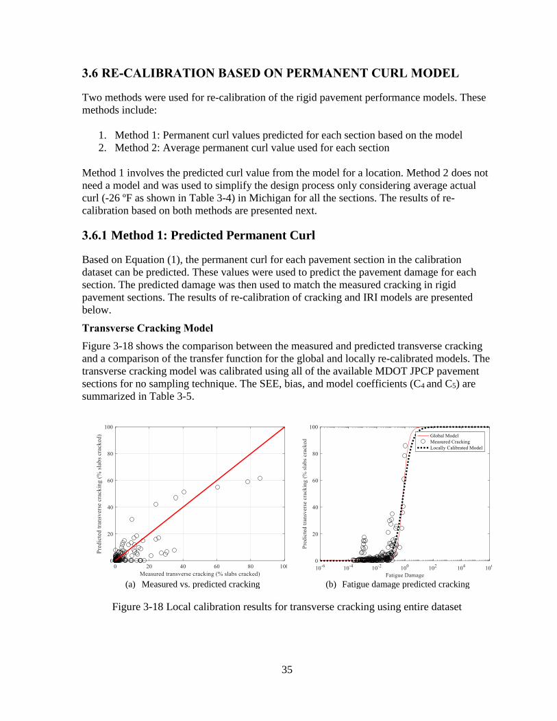
35
3.6 RE-CALIBRATION BASED ON PERMANENT CURL MODEL
Two methods were used for re-calibration of the rigid pavement performance models. These
methods include:
1. Method 1: Permanent curl values predicted for each section based on the model
2. Method 2: Average permanent curl value used for each section
Method 1 involves the predicted curl value from the model for a location. Method 2 does not
need a model and was used to simplify the design process only considering average actual
curl (-26 ºF as shown in Table 3-4) in Michigan for all the sections. The results of re-
calibration based on both methods are presented next.
3.6.1 Method 1: Predicted Permanent Curl
Based on Equation (1), the permanent curl for each pavement section in the calibration
dataset can be predicted. These values were used to predict the pavement damage for each
section. The predicted damage was then used to match the measured cracking in rigid
pavement sections. The results of re-calibration of cracking and IRI models are presented
below.
Transverse Cracking Model
Figure 3-18 shows the comparison between the measured and predicted transverse cracking
and a comparison of the transfer function for the global and locally re-calibrated models. The
transverse cracking model was calibrated using all of the available MDOT JPCP pavement
sections for no sampling technique. The SEE, bias, and model coefficients (C4 and C5) are
summarized in Table 3-5.
(a) Measured vs. predicted cracking
(b) Fatigue damage predicted cracking
Figure 3-18 Local calibration results for transverse cracking using entire dataset
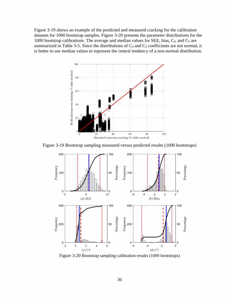
36
Figure 3-19 shows an example of the predicted and measured cracking for the calibration
datasets for 1000 bootstrap samples. Figure 3-20 presents the parameter distributions for the
1000 bootstrap calibrations. The average and median values for SEE, bias, C4, and C5 are
summarized in Table 3-5. Since the distributions of C4 and C5 coefficients are not normal, it
is better to use median values to represent the central tendency of a non-normal distribution.
Figure 3-19 Bootstrap sampling measured versus predicted results (1000 bootstraps)
Figure 3-20 Bootstrap sampling calibration results (1000 bootstraps)
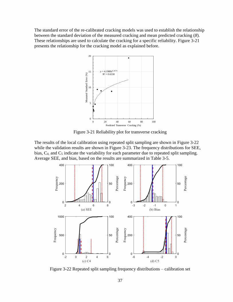
37
The standard error of the re-calibrated cracking models was used to establish the relationship
between the standard deviation of the measured cracking and mean predicted cracking (8).
These relationships are used to calculate the cracking for a specific reliability. Figure 3-21
presents the relationship for the cracking model as explained before.
Figure 3-21 Reliability plot for transverse cracking
The results of the local calibration using repeated split sampling are shown in Figure 3-22
while the validation results are shown in Figure 3-23. The frequency distributions for SEE,
bias, C4, and C5 indicate the variability for each parameter due to repeated split sampling.
Average SEE, and bias, based on the results are summarized in Table 3-5.
Figure 3-22 Repeated split sampling frequency distributions – calibration set
y = 4.1988x0.2674
R² = 0.6558
0
5
10
15
20
0 20 40 60 80 100
Mea
sure
d S
tand
ard E
rror
(%)
Predicted Transverse Cracking (%)
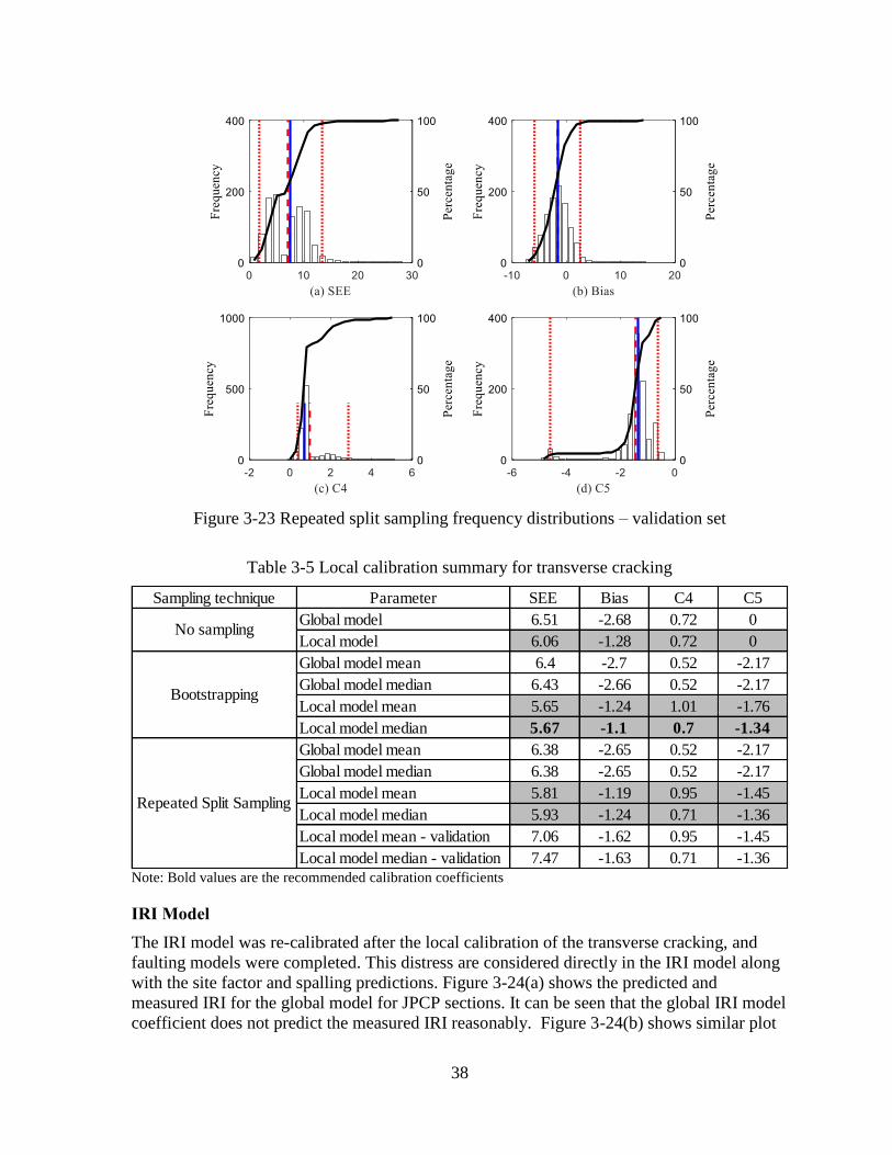
38
Figure 3-23 Repeated split sampling frequency distributions – validation set
Table 3-5 Local calibration summary for transverse cracking
Note: Bold values are the recommended calibration coefficients
IRI Model
The IRI model was re-calibrated after the local calibration of the transverse cracking, and
faulting models were completed. This distress are considered directly in the IRI model along
with the site factor and spalling predictions. Figure 3-24(a) shows the predicted and
measured IRI for the global model for JPCP sections. It can be seen that the global IRI model
coefficient does not predict the measured IRI reasonably. Figure 3-24(b) shows similar plot
Sampling technique Parameter SEE Bias C4 C5
Global model 6.51 -2.68 0.72 0
Local model 6.06 -1.28 0.72 0
Global model mean 6.4 -2.7 0.52 -2.17
Global model median 6.43 -2.66 0.52 -2.17
Local model mean 5.65 -1.24 1.01 -1.76
Local model median 5.67 -1.1 0.7 -1.34
Global model mean 6.38 -2.65 0.52 -2.17
Global model median 6.38 -2.65 0.52 -2.17
Local model mean 5.81 -1.19 0.95 -1.45
Local model median 5.93 -1.24 0.71 -1.36
Local model mean - validation 7.06 -1.62 0.95 -1.45
Local model median - validation 7.47 -1.63 0.71 -1.36
No sampling
Bootstrapping
Repeated Split Sampling
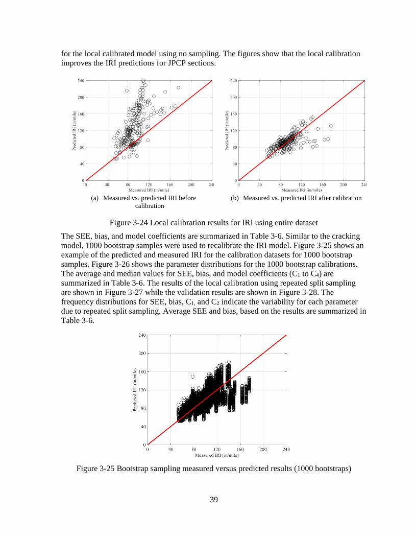
39
for the local calibrated model using no sampling. The figures show that the local calibration
improves the IRI predictions for JPCP sections.
(a) Measured vs. predicted IRI before
calibration
(b) Measured vs. predicted IRI after calibration
Figure 3-24 Local calibration results for IRI using entire dataset
The SEE, bias, and model coefficients are summarized in Table 3-6. Similar to the cracking
model, 1000 bootstrap samples were used to recalibrate the IRI model. Figure 3-25 shows an
example of the predicted and measured IRI for the calibration datasets for 1000 bootstrap
samples. Figure 3-26 shows the parameter distributions for the 1000 bootstrap calibrations.
The average and median values for SEE, bias, and model coefficients (C1 to C4) are
summarized in Table 3-6. The results of the local calibration using repeated split sampling
are shown in Figure 3-27 while the validation results are shown in Figure 3-28. The
frequency distributions for SEE, bias, C1, and C2 indicate the variability for each parameter
due to repeated split sampling. Average SEE and bias, based on the results are summarized in
Table 3-6.
Figure 3-25 Bootstrap sampling measured versus predicted results (1000 bootstraps)
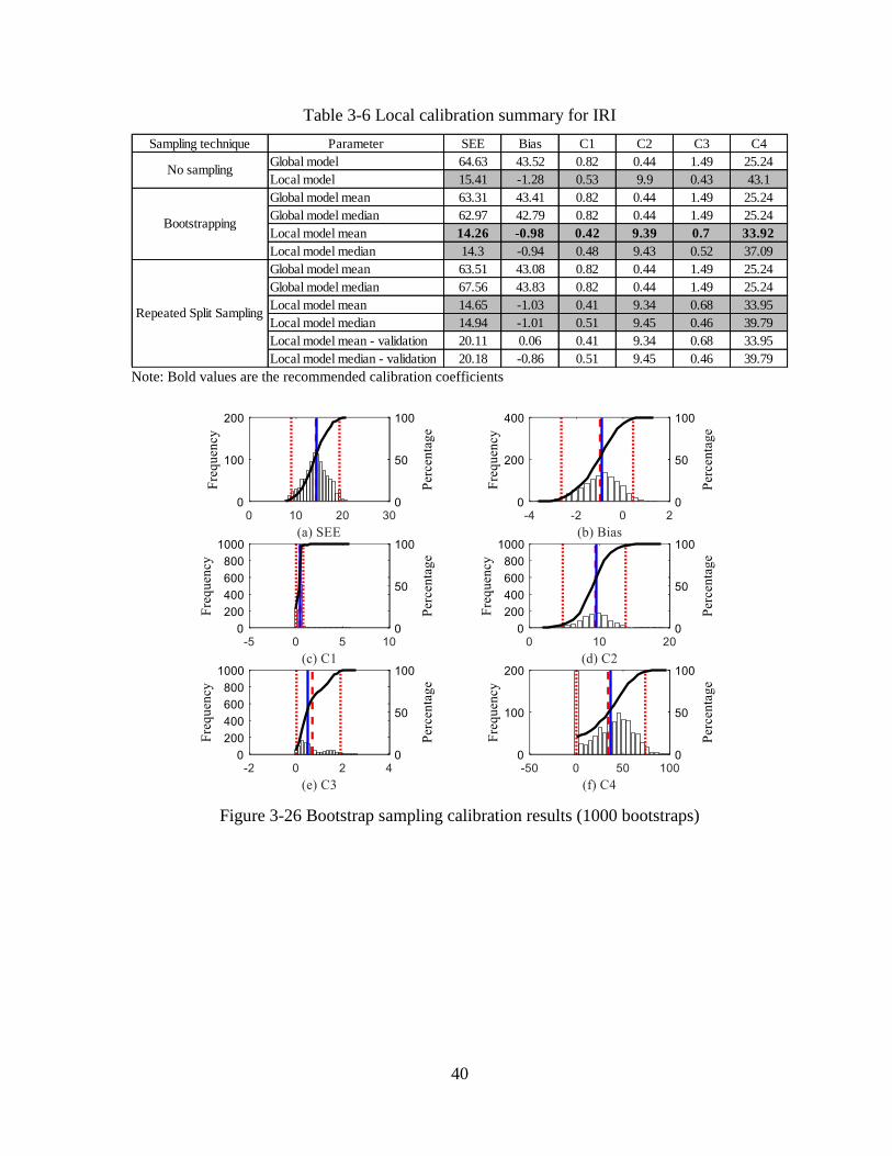
40
Table 3-6 Local calibration summary for IRI
Note: Bold values are the recommended calibration coefficients
Figure 3-26 Bootstrap sampling calibration results (1000 bootstraps)
Sampling technique Parameter SEE Bias C1 C2 C3 C4
Global model 64.63 43.52 0.82 0.44 1.49 25.24
Local model 15.41 -1.28 0.53 9.9 0.43 43.1
Global model mean 63.31 43.41 0.82 0.44 1.49 25.24
Global model median 62.97 42.79 0.82 0.44 1.49 25.24
Local model mean 14.26 -0.98 0.42 9.39 0.7 33.92
Local model median 14.3 -0.94 0.48 9.43 0.52 37.09
Global model mean 63.51 43.08 0.82 0.44 1.49 25.24
Global model median 67.56 43.83 0.82 0.44 1.49 25.24
Local model mean 14.65 -1.03 0.41 9.34 0.68 33.95
Local model median 14.94 -1.01 0.51 9.45 0.46 39.79
Local model mean - validation 20.11 0.06 0.41 9.34 0.68 33.95
Local model median - validation 20.18 -0.86 0.51 9.45 0.46 39.79
No sampling
Bootstrapping
Repeated Split Sampling
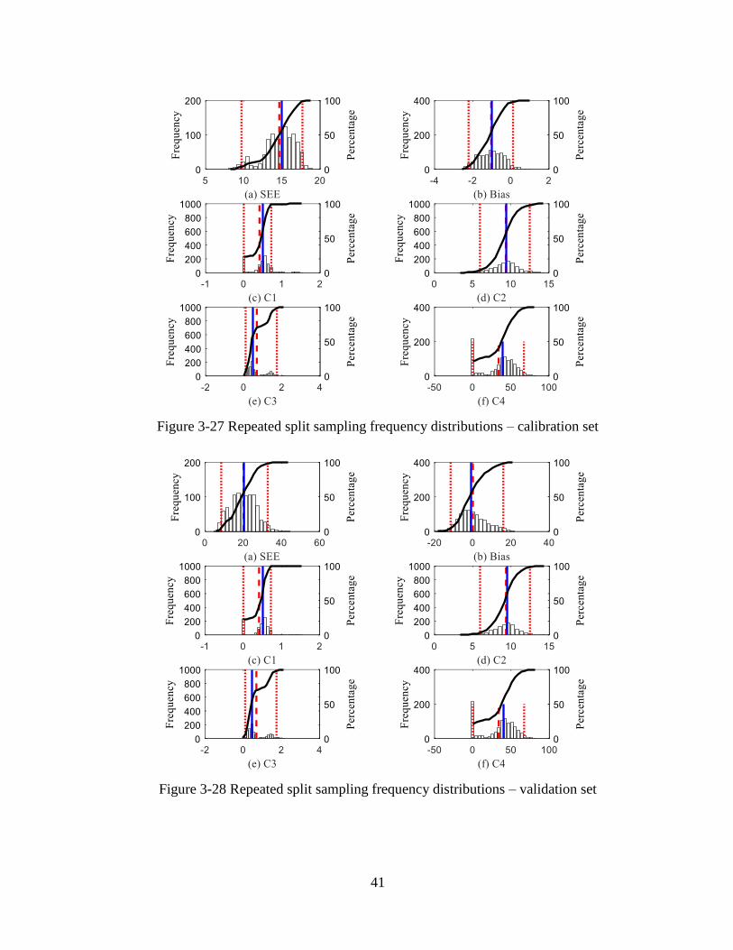
41
Figure 3-27 Repeated split sampling frequency distributions – calibration set
Figure 3-28 Repeated split sampling frequency distributions – validation set
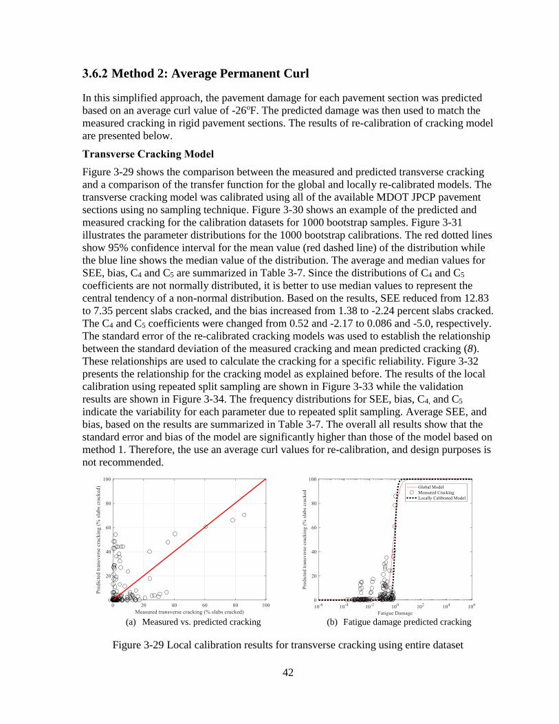
42
3.6.2 Method 2: Average Permanent Curl
In this simplified approach, the pavement damage for each pavement section was predicted
based on an average curl value of -26oF. The predicted damage was then used to match the
measured cracking in rigid pavement sections. The results of re-calibration of cracking model
are presented below.
Transverse Cracking Model
Figure 3-29 shows the comparison between the measured and predicted transverse cracking
and a comparison of the transfer function for the global and locally re-calibrated models. The
transverse cracking model was calibrated using all of the available MDOT JPCP pavement
sections using no sampling technique. Figure 3-30 shows an example of the predicted and
measured cracking for the calibration datasets for 1000 bootstrap samples. Figure 3-31
illustrates the parameter distributions for the 1000 bootstrap calibrations. The red dotted lines
show 95% confidence interval for the mean value (red dashed line) of the distribution while
the blue line shows the median value of the distribution. The average and median values for
SEE, bias, C4 and C5 are summarized in Table 3-7. Since the distributions of C4 and C5
coefficients are not normally distributed, it is better to use median values to represent the
central tendency of a non-normal distribution. Based on the results, SEE reduced from 12.83
to 7.35 percent slabs cracked, and the bias increased from 1.38 to -2.24 percent slabs cracked.
The C4 and C5 coefficients were changed from 0.52 and -2.17 to 0.086 and -5.0, respectively.
The standard error of the re-calibrated cracking models was used to establish the relationship
between the standard deviation of the measured cracking and mean predicted cracking (8).
These relationships are used to calculate the cracking for a specific reliability. Figure 3-32
presents the relationship for the cracking model as explained before. The results of the local
calibration using repeated split sampling are shown in Figure 3-33 while the validation
results are shown in Figure 3-34. The frequency distributions for SEE, bias, C4, and C5
indicate the variability for each parameter due to repeated split sampling. Average SEE, and
bias, based on the results are summarized in Table 3-7. The overall all results show that the
standard error and bias of the model are significantly higher than those of the model based on
method 1. Therefore, the use an average curl values for re-calibration, and design purposes is
not recommended.
(a) Measured vs. predicted cracking
(b) Fatigue damage predicted cracking
Figure 3-29 Local calibration results for transverse cracking using entire dataset
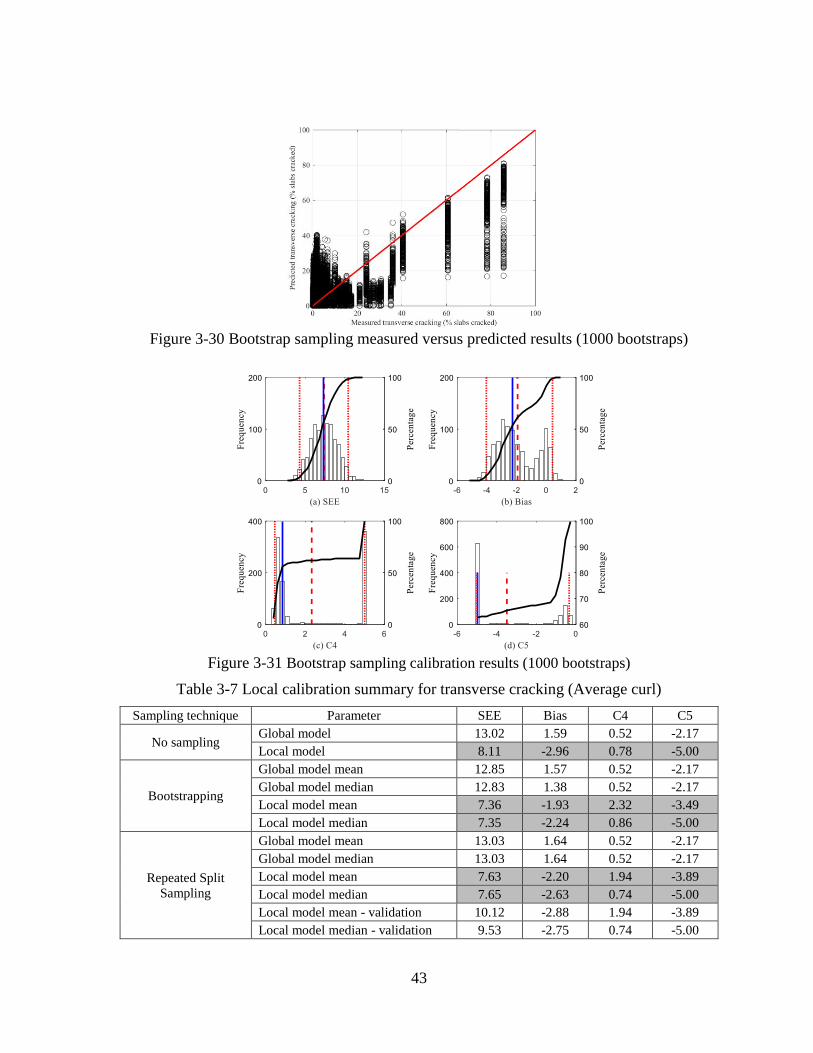
43
Figure 3-30 Bootstrap sampling measured versus predicted results (1000 bootstraps)
Figure 3-31 Bootstrap sampling calibration results (1000 bootstraps)
Table 3-7 Local calibration summary for transverse cracking (Average curl)
Sampling technique Parameter SEE Bias C4 C5
No sampling Global model 13.02 1.59 0.52 -2.17
Local model 8.11 -2.96 0.78 -5.00
Bootstrapping
Global model mean 12.85 1.57 0.52 -2.17
Global model median 12.83 1.38 0.52 -2.17
Local model mean 7.36 -1.93 2.32 -3.49
Local model median 7.35 -2.24 0.86 -5.00
Repeated Split
Sampling
Global model mean 13.03 1.64 0.52 -2.17
Global model median 13.03 1.64 0.52 -2.17
Local model mean 7.63 -2.20 1.94 -3.89
Local model median 7.65 -2.63 0.74 -5.00
Local model mean - validation 10.12 -2.88 1.94 -3.89
Local model median - validation 9.53 -2.75 0.74 -5.00
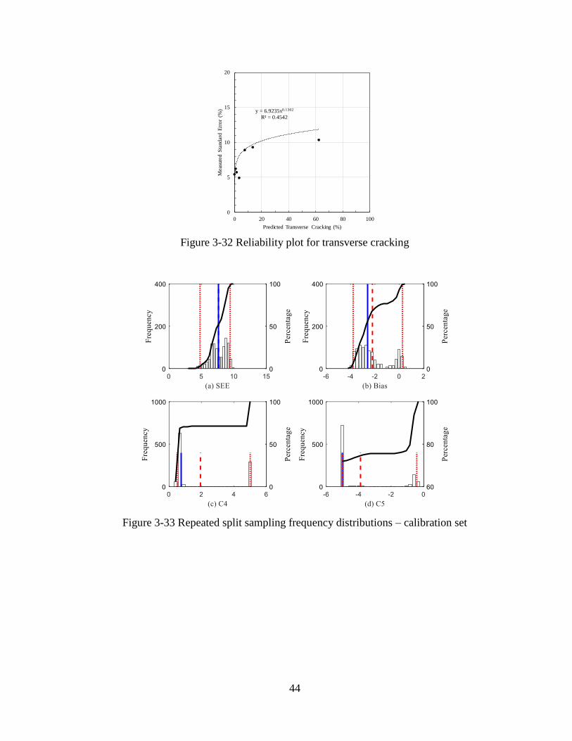
44
Figure 3-32 Reliability plot for transverse cracking
Figure 3-33 Repeated split sampling frequency distributions – calibration set
y = 6.9235x0.1302
R² = 0.4542
0
5
10
15
20
0 20 40 60 80 100M
easu
red
Sta
ndar
d E
rro
r (%
)
Predicted Transverse Cracking (%)
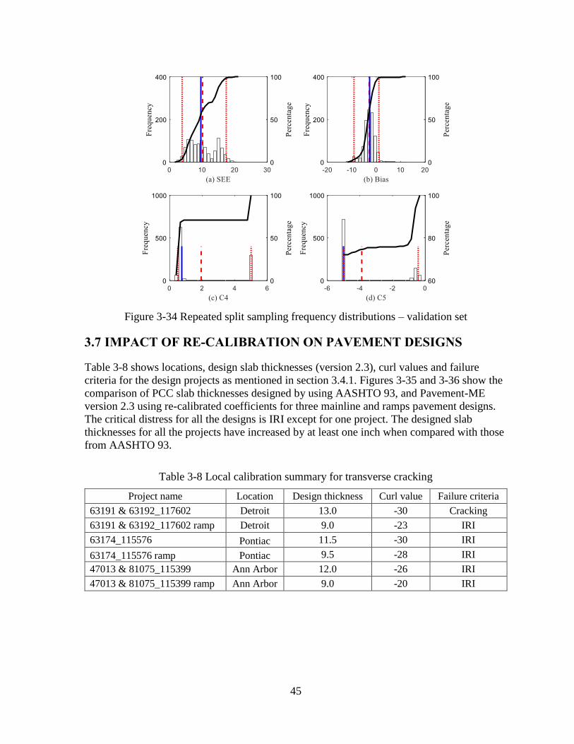
45
Figure 3-34 Repeated split sampling frequency distributions – validation set
3.7 IMPACT OF RE-CALIBRATION ON PAVEMENT DESIGNS
Table 3-8 shows locations, design slab thicknesses (version 2.3), curl values and failure
criteria for the design projects as mentioned in section 3.4.1. Figures 3-35 and 3-36 show the
comparison of PCC slab thicknesses designed by using AASHTO 93, and Pavement-ME
version 2.3 using re-calibrated coefficients for three mainline and ramps pavement designs.
The critical distress for all the designs is IRI except for one project. The designed slab
thicknesses for all the projects have increased by at least one inch when compared with those
from AASHTO 93.
Table 3-8 Local calibration summary for transverse cracking
Project name Location Design thickness Curl value Failure criteria
63191 & 63192_117602 Detroit 13.0 -30 Cracking
63191 & 63192_117602 ramp Detroit 9.0 -23 IRI
63174_115576 Pontiac 11.5 -30 IRI
63174_115576 ramp Pontiac 9.5 -28 IRI
47013 & 81075_115399 Ann Arbor 12.0 -26 IRI
47013 & 81075_115399 ramp Ann Arbor 9.0 -20 IRI
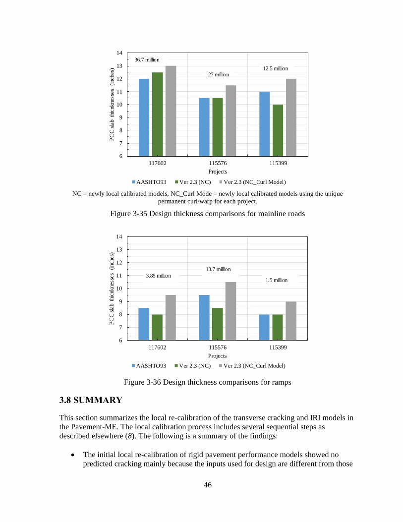
46
NC = newly local calibrated models, NC_Curl Mode = newly local calibrated models using the unique
permanent curl/warp for each project.
Figure 3-35 Design thickness comparisons for mainline roads
Figure 3-36 Design thickness comparisons for ramps
3.8 SUMMARY
This section summarizes the local re-calibration of the transverse cracking and IRI models in
the Pavement-ME. The local calibration process includes several sequential steps as
described elsewhere (8). The following is a summary of the findings:
The initial local re-calibration of rigid pavement performance models showed no
predicted cracking mainly because the inputs used for design are different from those
6
7
8
9
10
11
12
13
14
117602 115576 115399
PC
C s
lab t
hicn
kne
sses
(i
nche
s)
Projects
AASHTO93 Ver 2.3 (NC) Ver 2.3 (NC_Curl Model)
27 million12.5 million
36.7 million
6
7
8
9
10
11
12
13
14
117602 115576 115399
PC
C s
lab t
hicn
kne
sses
(inc
hes)
Projects
AASHTO93 Ver 2.3 (NC) Ver 2.3 (NC_Curl Model)
13.7 million
3.85 million1.5 million

47
used for re-calibration. For example, a compressive strength of 5600 psi is used in
design while an average value of 3500 psi (MOR = 560 psi) was used in initial re-
calibration.
All the previous ME designs showed no or very limited predicted cracking (i.e.,
negligible damage) and were controlled by IRI performance.
As a consequence, the performance models were re-calibrated using as-constructed
compressive strength (an average value of 5600 psi). Since there was no predicted
cracking using a permanent curl of -10oF (default value), the permanent curl was
varied to match the measured performance for each pavement section in the
calibration dataset.
Climate data, material properties, and design parameters were used to develop a
model for predicting permanent curl for each location. This model can be used at the
design stage to estimate permanent curl for a given location in Michigan.
The SEE and bias for the global models for cracking and IRI models are much higher
as compared to the locally re-calibrated models using all the selected pavement
sections (i.e., the entire dataset).
The main advantage of using resampling technique such as bootstrapping is to
quantify the variability (i.e., confidence interval) associated with the model
predictions and parameters. In addition, for a limited data set these techniques will
help in reducing the SEE and bias for the calibrated model.
The quantification of the variability will also help in determining a more robust
design reliability in the Pavement-ME.
Since the distributions of SEE and bias are non-normal, the median model
coefficients based on bootstrapping should be used. Those coefficients also showed
much lower SEE and bias than global coefficients for the cracking model.
The previously calibrated local joint faulting model coefficients are still valid based
on lowest SEE and bias and should be used.
The average IRI model coefficients using bootstrapping showed significantly lower
SEE and bias as compared to the global coefficients.
48
CHAPTER 4 - HMA THERMAL CRACKING MODEL
4.1 INTRODUCTION
Thermal cracking of flexible pavements is one of the leading causes of premature pavement
deterioration in regions of cold climate (where significant thermal fluctuations occur).
Thermal cracking is a not a load-associated distress, where a crack initiates in the pavement
structure due to localized thermally induced stress that exceeds the fracture resistance of the
mixture. Since daily and seasonal temperature variations tend to be extreme at the surface of
the pavement structure, the mechanism associated to thermal cracking is commonly
recognized as “top-down” transverse cracking. The primary concern for this type of distress
is the ingress of water through the crack into the pavement structure which can cause
stripping or formation of ice-lenses with the consequence of an early deterioration of the
asphalt concrete.
There are various thermal cracking models to predict the amount of cracking. Some
of the empirical models were developed between the early ‘70s and the late ‘80s and used
with varying degrees of success in the northern regions of the United States and in Canada
(14-17). However, none of these models could predict the amount of thermal cracking over
time. Later, the occurrence of thermal cracking has been associated with the asphalt binder
properties at low temperatures and the pavement design procedures were considering the
selection of mixes based on these properties (e.g., Performance Grade). However, these
characteristics are not enough to predict the thermo-mechanical behavior of an asphalt
mixture. A mechanics-based thermal cracking model was finally developed as part of the
SHRP A-005 research project. This model, named TC MODEL, could predict the thermal
cracking as a function of time and the AASHTOWare Pavement ME software uses its final
calibrated form for the prediction of this distress. It should be noted that the TC MODEL is
erroneously called “model” because this is based on a group of mathematical models that run
in a certain sequence to predict the amount of thermal cracking. The TC MODEL can be
divided into three clusters of models or modules: the input module, the pavement response
module, and the pavement distress module.
The input module has the main objective of calculating the hourly pavement
temperature profile using climate data and physical properties of the different HMAs used in
the pavement structure. The main inputs include fundamental properties of the asphalt mixes
as well as project-specific information (e.g., pavement structure and climatic data). These
data are used in the second module to predict the viscoelastic properties of the mixes (e.g.,
shift factors-temperature relationship and creep compliance master curve). Then, in the
pavement distress module, the stresses generated in the pavement structure are calculated and
the crack growth over time is predicted.
With the purpose of understanding the possible reasons for the extreme sensitivity of
the thermal cracking prediction with the TCMODEL, an analysis of the models implemented
in the pavement distress module is necessary. The TCMODEL is composed of three main
mathematical models: (i) the pavement response model to calculate the stress due to cooling
cycles, (ii) a mechanics-based model to determine the progression of a vertical crack (the
crack depth model), and (iii) the probabilistic model to determine the overall amount of
thermal cracking visible on the pavement surface (the crack amount model). The structural

49
response was originally modeled using a two-dimensional finite element program, known as
CRACKTIP. However, the excessive run times of this program made it unavailable for full
implementation in a pavement design process. Then, a regression analysis was carried out
using the CRACKTIP to simplify the determination of stresses generated into the pavement
structure by a cooling cycle. The result was the following simple equation for the calculation
of the stress intensity factor:
0.5600.45 1.99tipK C (1)
Where; K is the stress intensity factor, tip is the far-field pavement response at a depth of
crack tip (in psi), and 0C is the current crack length (in feet).
The amount of crack propagation into the pavement structure due to a given thermal
cycle is predicted using the so-called Paris law (18):
nC A K (2)
Where; C is the change in the crack depth due to a cooling cycle, K is the change in the
stress intensity factor due to a cooling cycle, A and n are the fracture parameters for a given
HMA mixture.
Given the form of the Equation (2) the fracture parameter A and n represent the
main material properties for the prediction of the amount of cracking. Based on Schapery’s
theory of crack propagation (19) these two parameters are directly correlated to (i) the slope
m of the linear portion of the creep compliance master curve (in log-log scale), (ii) the tensile
strength of the mix m , and (iii) the fracture energy density of the mixture. The experimental
investigation performed by Molenaar (20) resulted in the following equation for the fracture
parameter A :
log 4.389 2.52log( )mA E n (3)
or,
4.389 2.52 log( )
10 mE n
A
(4)
Where; E is the stiffness of the asphalt mixture, m the undamaged tensile strength
measured by performing the IDT test in the laboratory, and the n -value is a function of the
slope m of the linear portion of the creep compliance master curve (21):
1
0.8 1nm
(5)
The m -value to be used in Equation (5) can be easily obtained by fitting the creep compliance
master curve using the following equation:
0 1( ) ( )mD t D D t (6)
The presence of the asphalt mixture stiffness E in Equation (3) and (4) has been the subject
of many criticisms since the variable temperature conditions during the analysis lead to
variable E values. For this reason, the mix stiffness has been set equal to a constant value of
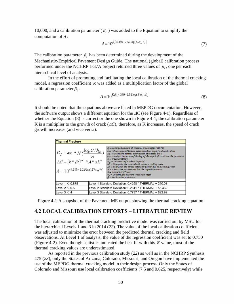
50
10,000, and a calibration parameter ( t ) was added to the Equation to simplify the
computation of A :
4.389 2.52log( )
10 t mE n
A
(7)
The calibration parameter t has been determined during the development of the
Mechanistic-Empirical Pavement Design Guide. The national (global) calibration process
performed under the NCHRP 1-37A project returned three values of t , one per each
hierarchical level of analysis.
In the effort of promoting and facilitating the local calibration of the thermal cracking
model, a regression coefficient K was added as a multiplication factor of the global
calibration parameter t :
4.389 2.52 log( )
10 t mK E n
A
(8)
It should be noted that the equations above are listed in MEPDG documentation. However,
the software output shows a different equation for the C (see Figure 4-1). Regardless of
whether the Equation (8) is correct or the one shown in Figure 4-1, the calibration parameter
K is a multiplier to the growth of crack (C), therefore, as K increases, the speed of crack
growth increases (and vice versa).
Figure 4-1 A snapshot of the Pavement ME output showing the thermal cracking equation
4.2 LOCAL CALIBRATION EFFORTS – LITERATURE REVIEW
The local calibration of the thermal cracking predictive model was carried out by MSU for
the hierarchical Levels 1 and 3 in 2014 (22). The value of the local calibration coefficient
was adjusted to minimize the error between the predicted thermal cracking and field
observations. At Level 1 of analysis, the value of the regression coefficient was set to 0.750
(Figure 4-2). Even though statistics indicated the best fit with this K value, most of the
thermal cracking values are underestimated.
As reported in the previous calibration study (22) as well as in the NCHRP Synthesis
475 (23), only the States of Arizona, Colorado, Missouri, and Oregon have implemented the
use of the MEPDG thermal cracking model in their design process. Only the States of
Colorado and Missouri use local calibration coefficients (7.5 and 0.625, respectively) while
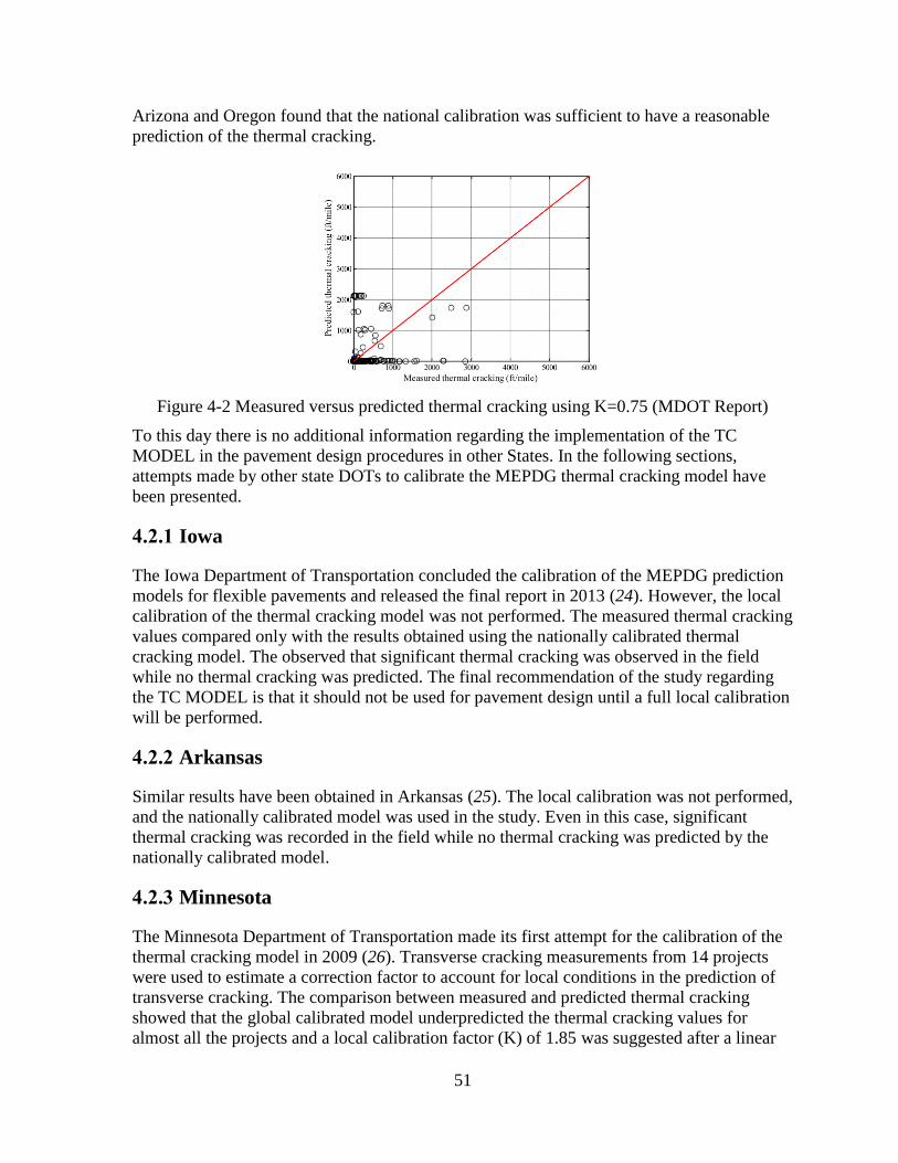
51
Arizona and Oregon found that the national calibration was sufficient to have a reasonable
prediction of the thermal cracking.
Figure 4-2 Measured versus predicted thermal cracking using K=0.75 (MDOT Report)
To this day there is no additional information regarding the implementation of the TC
MODEL in the pavement design procedures in other States. In the following sections,
attempts made by other state DOTs to calibrate the MEPDG thermal cracking model have
been presented.
4.2.1 Iowa
The Iowa Department of Transportation concluded the calibration of the MEPDG prediction
models for flexible pavements and released the final report in 2013 (24). However, the local
calibration of the thermal cracking model was not performed. The measured thermal cracking
values compared only with the results obtained using the nationally calibrated thermal
cracking model. The observed that significant thermal cracking was observed in the field
while no thermal cracking was predicted. The final recommendation of the study regarding
the TC MODEL is that it should not be used for pavement design until a full local calibration
will be performed.
4.2.2 Arkansas
Similar results have been obtained in Arkansas (25). The local calibration was not performed,
and the nationally calibrated model was used in the study. Even in this case, significant
thermal cracking was recorded in the field while no thermal cracking was predicted by the
nationally calibrated model.
4.2.3 Minnesota
The Minnesota Department of Transportation made its first attempt for the calibration of the
thermal cracking model in 2009 (26). Transverse cracking measurements from 14 projects
were used to estimate a correction factor to account for local conditions in the prediction of
transverse cracking. The comparison between measured and predicted thermal cracking
showed that the global calibrated model underpredicted the thermal cracking values for
almost all the projects and a local calibration factor (K) of 1.85 was suggested after a linear
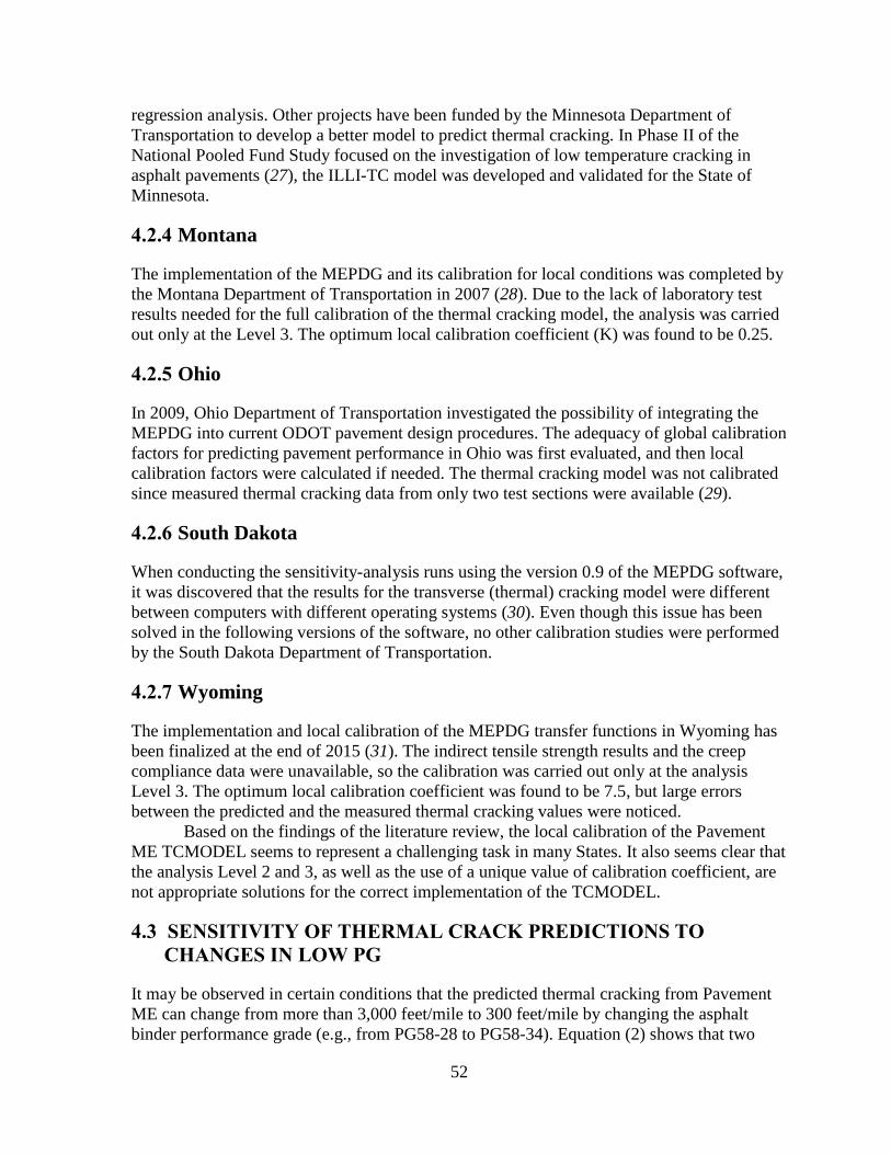
52
regression analysis. Other projects have been funded by the Minnesota Department of
Transportation to develop a better model to predict thermal cracking. In Phase II of the
National Pooled Fund Study focused on the investigation of low temperature cracking in
asphalt pavements (27), the ILLI-TC model was developed and validated for the State of
Minnesota.
4.2.4 Montana
The implementation of the MEPDG and its calibration for local conditions was completed by
the Montana Department of Transportation in 2007 (28). Due to the lack of laboratory test
results needed for the full calibration of the thermal cracking model, the analysis was carried
out only at the Level 3. The optimum local calibration coefficient (K) was found to be 0.25.
4.2.5 Ohio
In 2009, Ohio Department of Transportation investigated the possibility of integrating the
MEPDG into current ODOT pavement design procedures. The adequacy of global calibration
factors for predicting pavement performance in Ohio was first evaluated, and then local
calibration factors were calculated if needed. The thermal cracking model was not calibrated
since measured thermal cracking data from only two test sections were available (29).
4.2.6 South Dakota
When conducting the sensitivity-analysis runs using the version 0.9 of the MEPDG software,
it was discovered that the results for the transverse (thermal) cracking model were different
between computers with different operating systems (30). Even though this issue has been
solved in the following versions of the software, no other calibration studies were performed
by the South Dakota Department of Transportation.
4.2.7 Wyoming
The implementation and local calibration of the MEPDG transfer functions in Wyoming has
been finalized at the end of 2015 (31). The indirect tensile strength results and the creep
compliance data were unavailable, so the calibration was carried out only at the analysis
Level 3. The optimum local calibration coefficient was found to be 7.5, but large errors
between the predicted and the measured thermal cracking values were noticed.
Based on the findings of the literature review, the local calibration of the Pavement
ME TCMODEL seems to represent a challenging task in many States. It also seems clear that
the analysis Level 2 and 3, as well as the use of a unique value of calibration coefficient, are
not appropriate solutions for the correct implementation of the TCMODEL.
4.3 SENSITIVITY OF THERMAL CRACK PREDICTIONS TO
CHANGES IN LOW PG
It may be observed in certain conditions that the predicted thermal cracking from Pavement
ME can change from more than 3,000 feet/mile to 300 feet/mile by changing the asphalt
binder performance grade (e.g., from PG58-28 to PG58-34). Equation (2) shows that two

53
main material parameters are controlling the growth of thermal cracking; A and n. Among
other factors, one of the factors affecting the parameter n is the low-temperature PG of the
binder. In general, as PG decreases (e.g., from PG58-28 to PG58-34), the n also decreases
(see Table 4-1). Since n is in the power of stress intensity factor (K), small changes in n
effect the thermal crack growth (C) significantly. Table 4-1 shows the fracture properties
(m, n and IDT strength) of eight asphalt mixtures used in MDOT roadways. Only PGs of the
asphalt mixtures were shown here for brevity. As shown, as the low PG decreases (column
(i)), the n decreases (column (iii)). For a given K (see column (v), where 0.75 is the Level 1
calibration coefficient used in Michigan), when PG decreases by one grade, C decreases by
90-100% (see columns (vi) and (vii)). However, when a mix specific K is used (column
(viii)), C decreases to a lesser extent (see columns (ix) and (x)), which is more logical.
Therefore, it is essential to treat the K as a major mix-specific input to be able to predict the
field behavior accurately.
Table 4-1 Effect of PG on the fracture properties of an asphalt layer
4.4 RE-EVALUATION OF TC MODEL ON LIMITED NUMBER OF
MDOT PROJECTS
4.4.1 Project Selection
To re-evaluate the TC MODEL using the latest distress data from Michigan roadways,
twenty (20) in-service pavement sections were selected. These pavement sections represent
common flexible pavement types and materials used by MDOT. The pavement sections had
the following characteristics:
Binder
Performance
Grade (PG)
m n
IDT
Strength
(psi)
K C
% change
in C
with
respect to
previous
PG
K(1) C
% change
in C
with
respect to
previous
PG
(i) (ii) (iii) (iv) (v) (vi) (vii) (viii) (ix) (x)
PG58-22 0.11 8.07 463 0.75 1.57E-19 N/A 0.75 1.57E-19 N/A
PG58-28 0.12 7.47 470 0.75 1.84E-20 -88.3% 0.735 8.97E-20 -43.0%
PG58-34 0.16 5.80 474 0.75 9.76E-23 -99.5% 0.69 4.60E-20 -48.7%
PG64-22 0.09 9.69 549 0.75 8.44E-18 N/A 0.75 8.44E-18 N/A
PG64-28 0.13 6.95 484 0.75 2.68E-21 -100.0% 0.74 7.66E-21 -99.9%
PG64-34 0.16 5.80 466 0.75 1.15E-22 -95.7% 0.73 8.88E-22 -88.4%
PG70-22 0.08 10.80 607 0.75 1.79E-16 N/A 0.75 1.79E-16 N/A
PG70-28 0.11 8.07 518 0.75 5.45E-20 -100.0% 0.68 1.04E-16 -42.1% (1) These values do not represent the result of any calibration process. They were selected with the only purpose of showing the effect of different
K values on the prediction of thermal cracking.
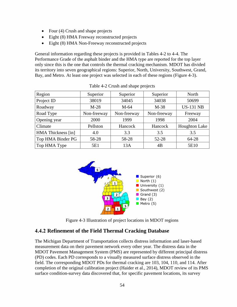
54
Four (4) Crush and shape projects
Eight (8) HMA Freeway reconstructed projects
Eight (8) HMA Non-Freeway reconstructed projects
General information regarding these projects is provided in Tables 4-2 to 4-4. The
Performance Grade of the asphalt binder and the HMA type are reported for the top layer
only since this is the one that controls the thermal cracking mechanism. MDOT has divided
its territory into seven geographical regions: Superior, North, University, Southwest, Grand,
Bay, and Metro. At least one project was selected in each of these regions (Figure 4-3).
Table 4-2 Crush and shape projects
Region Superior Superior Superior North
Project ID 38019 34045 34038 50699
Roadway M-28 M-64 M-38 US-131 NB
Road Type Non-freeway Non-freeway Non-freeway Freeway
Opening year 2000 1999 1998 2004
Climate Pellston Hancock Hancock Houghton Lake
HMA Thickness [in] 4.0 3.3 3.5 3.5
Top HMA Binder PG 58-28 58-28 52-28 64-28
Top HMA Type 5E1 13A 4B 5E10
Figure 4-3 Illustration of project locations in MDOT regions
4.4.2 Refinement of the Field Thermal Cracking Database
The Michigan Department of Transportation collects distress information and laser-based
measurement data on their pavement network every other year. The distress data in the
MDOT Pavement Management System (PMS) are represented by different principal distress
(PD) codes. Each PD corresponds to a visually measured surface distress observed in the
field. The corresponding MDOT PDs for thermal cracking are 103, 104, 110, and 114. After
completion of the original calibration project (Haider et al., 2014), MDOT review of its PMS
surface condition-survey data discovered that, for specific pavement locations, its survey
6
1
23
512
Superior (6)
North (1)
University (1)
Southwest (2)
Grand (3)
Bay (2)
Metro (5)
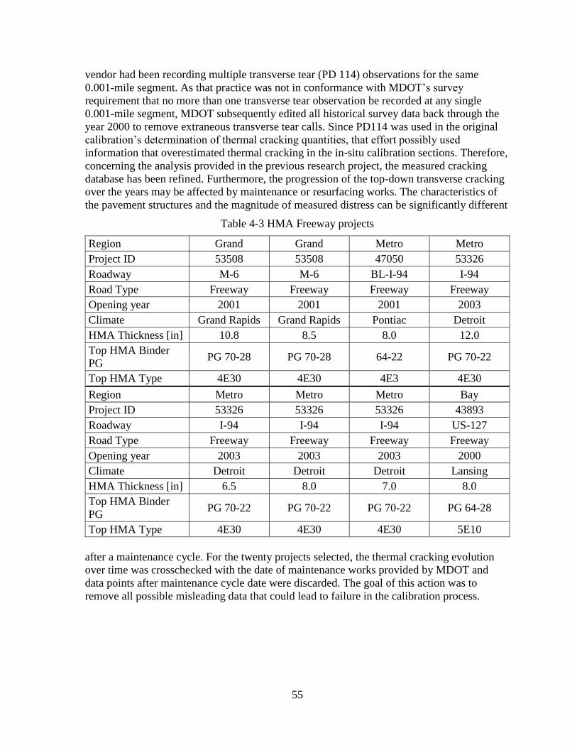
55
vendor had been recording multiple transverse tear (PD 114) observations for the same
0.001-mile segment. As that practice was not in conformance with MDOT’s survey
requirement that no more than one transverse tear observation be recorded at any single
0.001-mile segment, MDOT subsequently edited all historical survey data back through the
year 2000 to remove extraneous transverse tear calls. Since PD114 was used in the original
calibration’s determination of thermal cracking quantities, that effort possibly used
information that overestimated thermal cracking in the in-situ calibration sections. Therefore,
concerning the analysis provided in the previous research project, the measured cracking
database has been refined. Furthermore, the progression of the top-down transverse cracking
over the years may be affected by maintenance or resurfacing works. The characteristics of
the pavement structures and the magnitude of measured distress can be significantly different
Table 4-3 HMA Freeway projects
Region Grand Grand Metro Metro
Project ID 53508 53508 47050 53326
Roadway M-6 M-6 BL-I-94 I-94
Road Type Freeway Freeway Freeway Freeway
Opening year 2001 2001 2001 2003
Climate Grand Rapids Grand Rapids Pontiac Detroit
HMA Thickness [in] 10.8 8.5 8.0 12.0
Top HMA Binder
PG PG 70-28 PG 70-28 64-22 PG 70-22
Top HMA Type 4E30 4E30 4E3 4E30
Region Metro Metro Metro Bay
Project ID 53326 53326 53326 43893
Roadway I-94 I-94 I-94 US-127
Road Type Freeway Freeway Freeway Freeway
Opening year 2003 2003 2003 2000
Climate Detroit Detroit Detroit Lansing
HMA Thickness [in] 6.5 8.0 7.0 8.0
Top HMA Binder
PG PG 70-22 PG 70-22 PG 70-22 PG 64-28
Top HMA Type 4E30 4E30 4E30 5E10
after a maintenance cycle. For the twenty projects selected, the thermal cracking evolution
over time was crosschecked with the date of maintenance works provided by MDOT and
data points after maintenance cycle date were discarded. The goal of this action was to
remove all possible misleading data that could lead to failure in the calibration process.
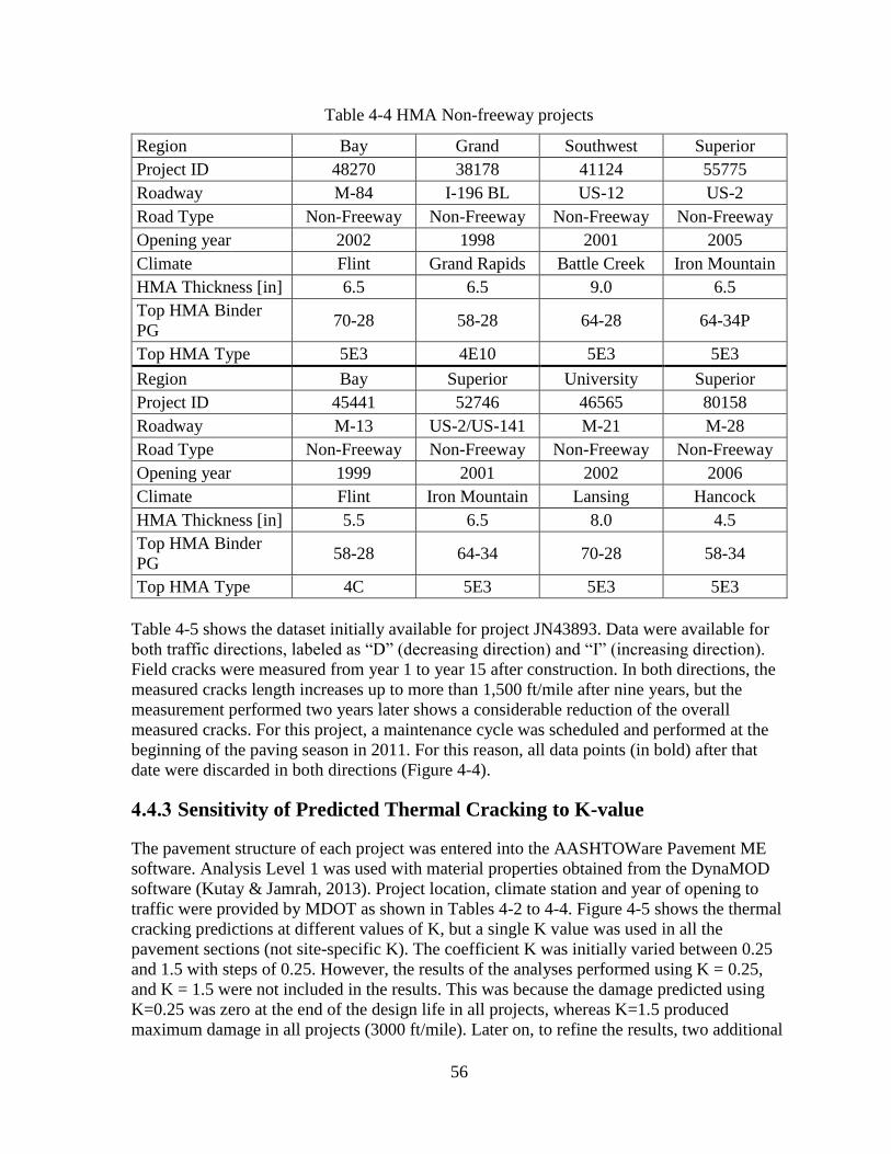
56
Table 4-4 HMA Non-freeway projects
Region Bay Grand Southwest Superior
Project ID 48270 38178 41124 55775
Roadway M-84 I-196 BL US-12 US-2
Road Type Non-Freeway Non-Freeway Non-Freeway Non-Freeway
Opening year 2002 1998 2001 2005
Climate Flint Grand Rapids Battle Creek Iron Mountain
HMA Thickness [in] 6.5 6.5 9.0 6.5
Top HMA Binder
PG 70-28 58-28 64-28 64-34P
Top HMA Type 5E3 4E10 5E3 5E3
Region Bay Superior University Superior
Project ID 45441 52746 46565 80158
Roadway M-13 US-2/US-141 M-21 M-28
Road Type Non-Freeway Non-Freeway Non-Freeway Non-Freeway
Opening year 1999 2001 2002 2006
Climate Flint Iron Mountain Lansing Hancock
HMA Thickness [in] 5.5 6.5 8.0 4.5
Top HMA Binder
PG 58-28 64-34 70-28 58-34
Top HMA Type 4C 5E3 5E3 5E3
Table 4-5 shows the dataset initially available for project JN43893. Data were available for
both traffic directions, labeled as “D” (decreasing direction) and “I” (increasing direction).
Field cracks were measured from year 1 to year 15 after construction. In both directions, the
measured cracks length increases up to more than 1,500 ft/mile after nine years, but the
measurement performed two years later shows a considerable reduction of the overall
measured cracks. For this project, a maintenance cycle was scheduled and performed at the
beginning of the paving season in 2011. For this reason, all data points (in bold) after that
date were discarded in both directions (Figure 4-4).
4.4.3 Sensitivity of Predicted Thermal Cracking to K-value
The pavement structure of each project was entered into the AASHTOWare Pavement ME
software. Analysis Level 1 was used with material properties obtained from the DynaMOD
software (Kutay & Jamrah, 2013). Project location, climate station and year of opening to
traffic were provided by MDOT as shown in Tables 4-2 to 4-4. Figure 4-5 shows the thermal
cracking predictions at different values of K, but a single K value was used in all the
pavement sections (not site-specific K). The coefficient K was initially varied between 0.25
and 1.5 with steps of 0.25. However, the results of the analyses performed using K = 0.25,
and K = 1.5 were not included in the results. This was because the damage predicted using
K=0.25 was zero at the end of the design life in all projects, whereas K=1.5 produced
maximum damage in all projects (3000 ft/mile). Later on, to refine the results, two additional
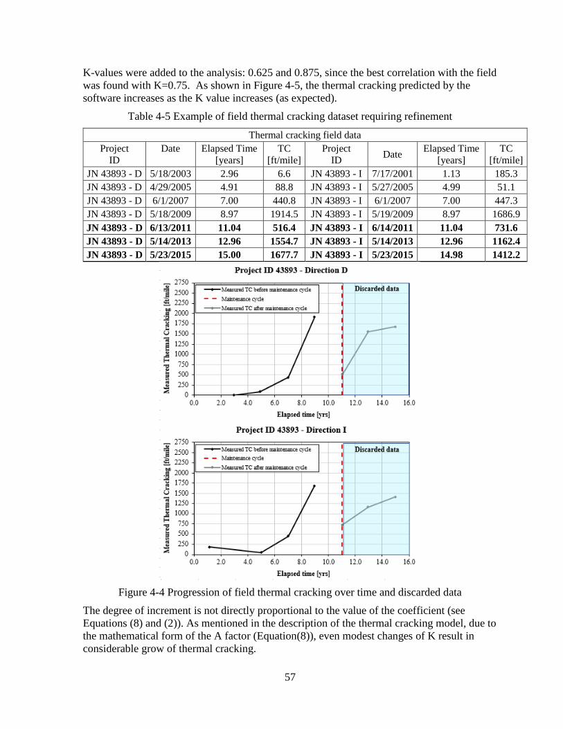
57
K-values were added to the analysis: 0.625 and 0.875, since the best correlation with the field
was found with K=0.75. As shown in Figure 4-5, the thermal cracking predicted by the
software increases as the K value increases (as expected).
Table 4-5 Example of field thermal cracking dataset requiring refinement
Thermal cracking field data
Project
ID
Date
Elapsed Time
[years]
TC
[ft/mile]
Project
ID Date
Elapsed Time
[years]
TC
[ft/mile]
JN 43893 - D 5/18/2003 2.96 6.6 JN 43893 - I 7/17/2001 1.13 185.3
JN 43893 - D 4/29/2005 4.91 88.8 JN 43893 - I 5/27/2005 4.99 51.1
JN 43893 - D 6/1/2007 7.00 440.8 JN 43893 - I 6/1/2007 7.00 447.3
JN 43893 - D 5/18/2009 8.97 1914.5 JN 43893 - I 5/19/2009 8.97 1686.9
JN 43893 - D 6/13/2011 11.04 516.4 JN 43893 - I 6/14/2011 11.04 731.6
JN 43893 - D 5/14/2013 12.96 1554.7 JN 43893 - I 5/14/2013 12.96 1162.4
JN 43893 - D 5/23/2015 15.00 1677.7 JN 43893 - I 5/23/2015 14.98 1412.2
Figure 4-4 Progression of field thermal cracking over time and discarded data
The degree of increment is not directly proportional to the value of the coefficient (see
Equations (8) and (2)). As mentioned in the description of the thermal cracking model, due to
the mathematical form of the A factor (Equation(8)), even modest changes of K result in
considerable grow of thermal cracking.

58
Figure 4-5 Predicted versus measured thermal cracking with various K values
The accuracy of the predictions was evaluated based on the average of the errors and the
standard error of the estimates (SEE):
p my y
ErrorN
(9)
2
p my ySEE
N
(10)
where: py is the thermal cracking predicted by the Pavement ME software, my is the measured
thermal cracking in the field, and N is the number of observations.
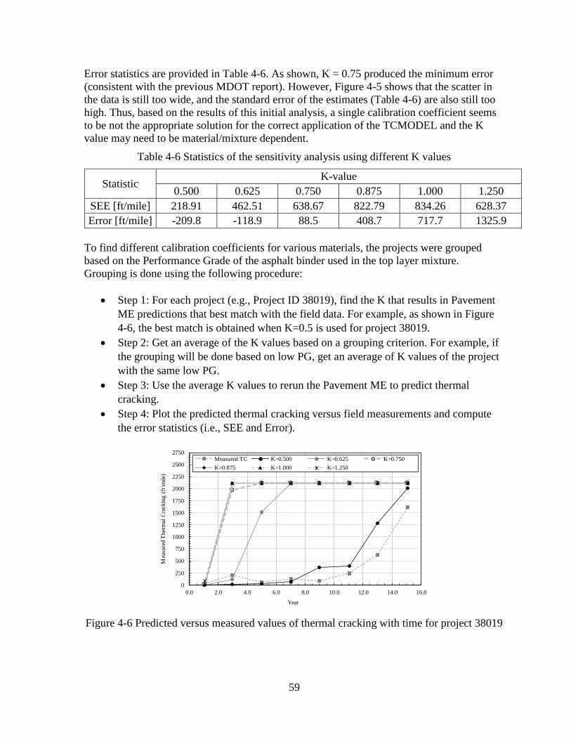
59
Error statistics are provided in Table 4-6. As shown, K = 0.75 produced the minimum error
(consistent with the previous MDOT report). However, Figure 4-5 shows that the scatter in
the data is still too wide, and the standard error of the estimates (Table 4-6) are also still too
high. Thus, based on the results of this initial analysis, a single calibration coefficient seems
to be not the appropriate solution for the correct application of the TCMODEL and the K
value may need to be material/mixture dependent.
Table 4-6 Statistics of the sensitivity analysis using different K values
Statistic K-value
0.500 0.625 0.750 0.875 1.000 1.250
SEE [ft/mile] 218.91 462.51 638.67 822.79 834.26 628.37
Error [ft/mile] -209.8 -118.9 88.5 408.7 717.7 1325.9
To find different calibration coefficients for various materials, the projects were grouped
based on the Performance Grade of the asphalt binder used in the top layer mixture.
Grouping is done using the following procedure:
Step 1: For each project (e.g., Project ID 38019), find the K that results in Pavement
ME predictions that best match with the field data. For example, as shown in Figure
4-6, the best match is obtained when K=0.5 is used for project 38019.
Step 2: Get an average of the K values based on a grouping criterion. For example, if
the grouping will be done based on low PG, get an average of K values of the project
with the same low PG.
Step 3: Use the average K values to rerun the Pavement ME to predict thermal
cracking.
Step 4: Plot the predicted thermal cracking versus field measurements and compute
the error statistics (i.e., SEE and Error).
Figure 4-6 Predicted versus measured values of thermal cracking with time for project 38019
0
250
500
750
1000
1250
1500
1750
2000
2250
2500
2750
0.0 2.0 4.0 6.0 8.0 10.0 12.0 14.0 16.0
Mea
sure
d T
her
mal
Cra
ckin
g (f
t\m
ile)
Year
Measured TC K=0.500 K=0.625 K=0.750
K=0.875 K=1.000 K=1.250
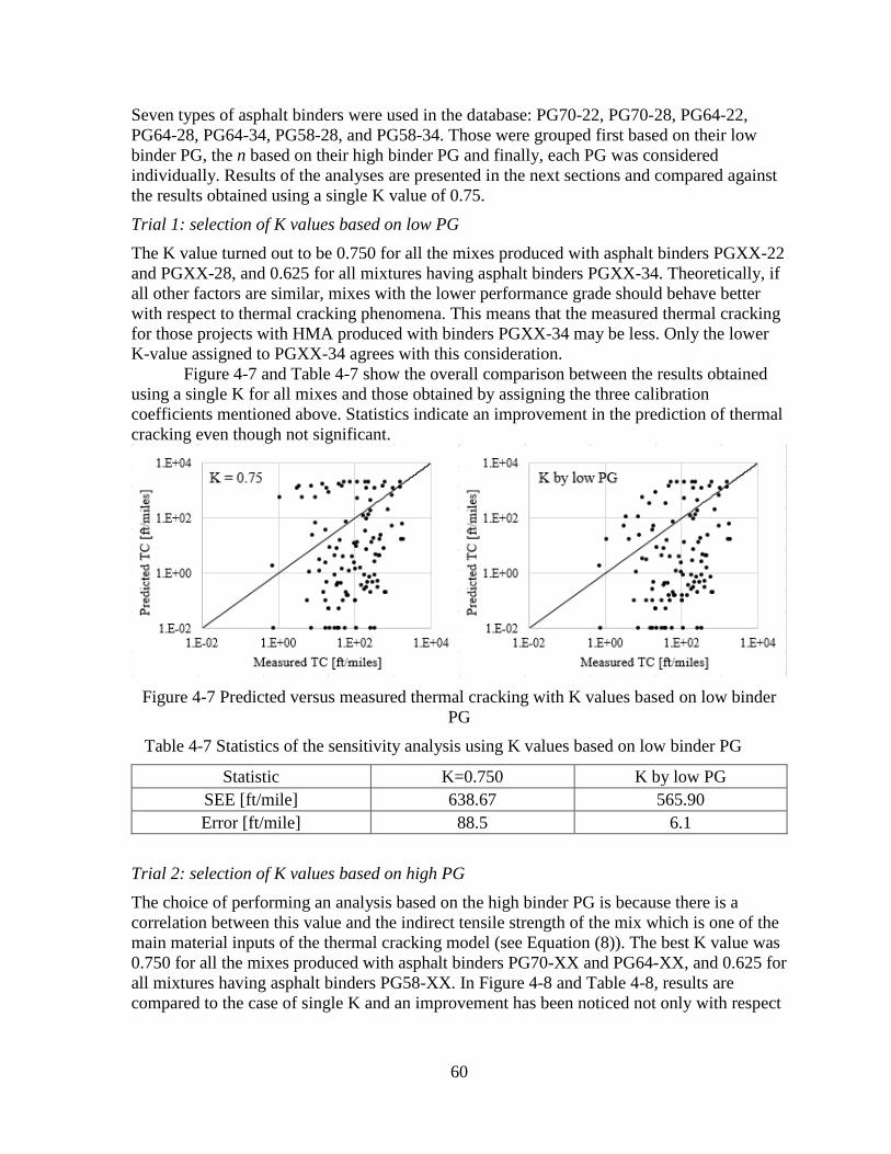
60
Seven types of asphalt binders were used in the database: PG70-22, PG70-28, PG64-22,
PG64-28, PG64-34, PG58-28, and PG58-34. Those were grouped first based on their low
binder PG, the n based on their high binder PG and finally, each PG was considered
individually. Results of the analyses are presented in the next sections and compared against
the results obtained using a single K value of 0.75.
Trial 1: selection of K values based on low PG
The K value turned out to be 0.750 for all the mixes produced with asphalt binders PGXX-22
and PGXX-28, and 0.625 for all mixtures having asphalt binders PGXX-34. Theoretically, if
all other factors are similar, mixes with the lower performance grade should behave better
with respect to thermal cracking phenomena. This means that the measured thermal cracking
for those projects with HMA produced with binders PGXX-34 may be less. Only the lower
K-value assigned to PGXX-34 agrees with this consideration.
Figure 4-7 and Table 4-7 show the overall comparison between the results obtained
using a single K for all mixes and those obtained by assigning the three calibration
coefficients mentioned above. Statistics indicate an improvement in the prediction of thermal
cracking even though not significant.
Figure 4-7 Predicted versus measured thermal cracking with K values based on low binder
PG
Table 4-7 Statistics of the sensitivity analysis using K values based on low binder PG
Statistic K=0.750 K by low PG
SEE [ft/mile] 638.67 565.90
Error [ft/mile] 88.5 6.1
Trial 2: selection of K values based on high PG
The choice of performing an analysis based on the high binder PG is because there is a
correlation between this value and the indirect tensile strength of the mix which is one of the
main material inputs of the thermal cracking model (see Equation (8)). The best K value was
0.750 for all the mixes produced with asphalt binders PG70-XX and PG64-XX, and 0.625 for
all mixtures having asphalt binders PG58-XX. In Figure 4-8 and Table 4-8, results are
compared to the case of single K and an improvement has been noticed not only with respect
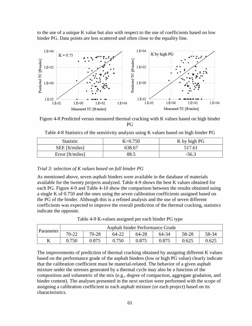
61
to the use of a unique K value but also with respect to the use of coefficients based on low
binder PG. Data points are less scattered and often close to the equality line.
Figure 4-8 Predicted versus measured thermal cracking with K values based on high binder
PG
Table 4-8 Statistics of the sensitivity analysis using K values based on high binder PG
Statistic K=0.750 K by high PG
SEE [ft/miles] 638.67 517.61
Error [ft/miles] 88.5 -56.3
Trial 3: selection of K values based on full binder PG
As mentioned above, seven asphalt binders were available in the database of materials
available for the twenty projects analyzed. Table 4-9 shows the best K values obtained for
each PG. Figure 4-9 and Table 4-10 show the comparison between the results obtained using
a single K of 0.750 and the ones using the seven calibration coefficients assigned based on
the PG of the binder. Although this is a refined analysis and the use of seven different
coefficients was expected to improve the overall prediction of the thermal cracking, statistics
indicate the opposite.
Table 4-9 K-values assigned per each binder PG type
Parameter Asphalt binder Performance Grade
70-22 70-28 64-22 64-28 64-34 58-28 58-34
K 0.750 0.875 0.750 0.875 0.875 0.625 0.625
The improvements of prediction of thermal cracking obtained by assigning different K values
based on the performance grade of the asphalt binders (low or high PG value) clearly indicate
that the calibration coefficient must be material-related. The behavior of a given asphalt
mixture under the stresses generated by a thermal cycle may also be a function of the
composition and volumetric of the mix (e.g., degree of compaction, aggregate gradation, and
binder content). The analyses presented in the next section were performed with the scope of
assigning a calibration coefficient to each asphalt mixture (or each project) based on its
characteristics.
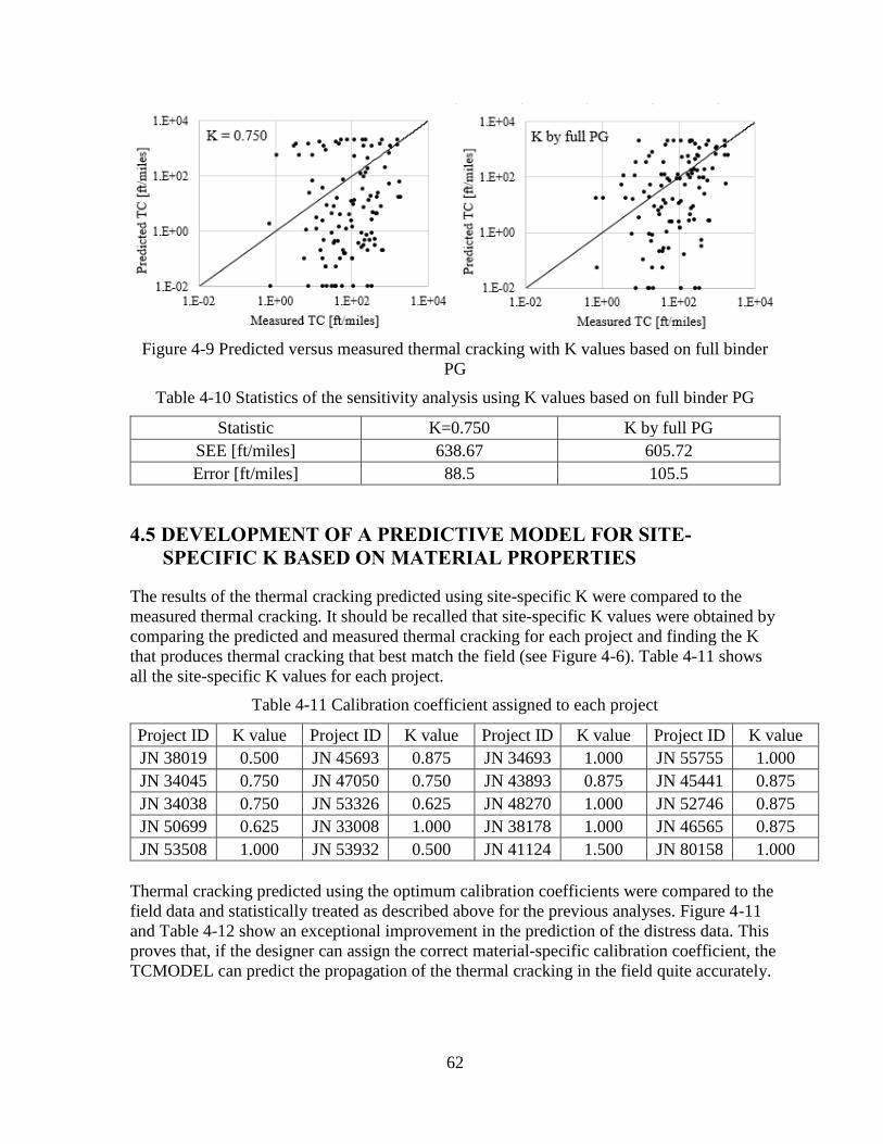
62
Figure 4-9 Predicted versus measured thermal cracking with K values based on full binder
PG
Table 4-10 Statistics of the sensitivity analysis using K values based on full binder PG
Statistic K=0.750 K by full PG
SEE [ft/miles] 638.67 605.72
Error [ft/miles] 88.5 105.5
4.5 DEVELOPMENT OF A PREDICTIVE MODEL FOR SITE-
SPECIFIC K BASED ON MATERIAL PROPERTIES
The results of the thermal cracking predicted using site-specific K were compared to the
measured thermal cracking. It should be recalled that site-specific K values were obtained by
comparing the predicted and measured thermal cracking for each project and finding the K
that produces thermal cracking that best match the field (see Figure 4-6). Table 4-11 shows
all the site-specific K values for each project.
Table 4-11 Calibration coefficient assigned to each project
Project ID K value Project ID K value Project ID K value Project ID K value
JN 38019 0.500 JN 45693 0.875 JN 34693 1.000 JN 55755 1.000
JN 34045 0.750 JN 47050 0.750 JN 43893 0.875 JN 45441 0.875
JN 34038 0.750 JN 53326 0.625 JN 48270 1.000 JN 52746 0.875
JN 50699 0.625 JN 33008 1.000 JN 38178 1.000 JN 46565 0.875
JN 53508 1.000 JN 53932 0.500 JN 41124 1.500 JN 80158 1.000
Thermal cracking predicted using the optimum calibration coefficients were compared to the
field data and statistically treated as described above for the previous analyses. Figure 4-11
and Table 4-12 show an exceptional improvement in the prediction of the distress data. This
proves that, if the designer can assign the correct material-specific calibration coefficient, the
TCMODEL can predict the propagation of the thermal cracking in the field quite accurately.
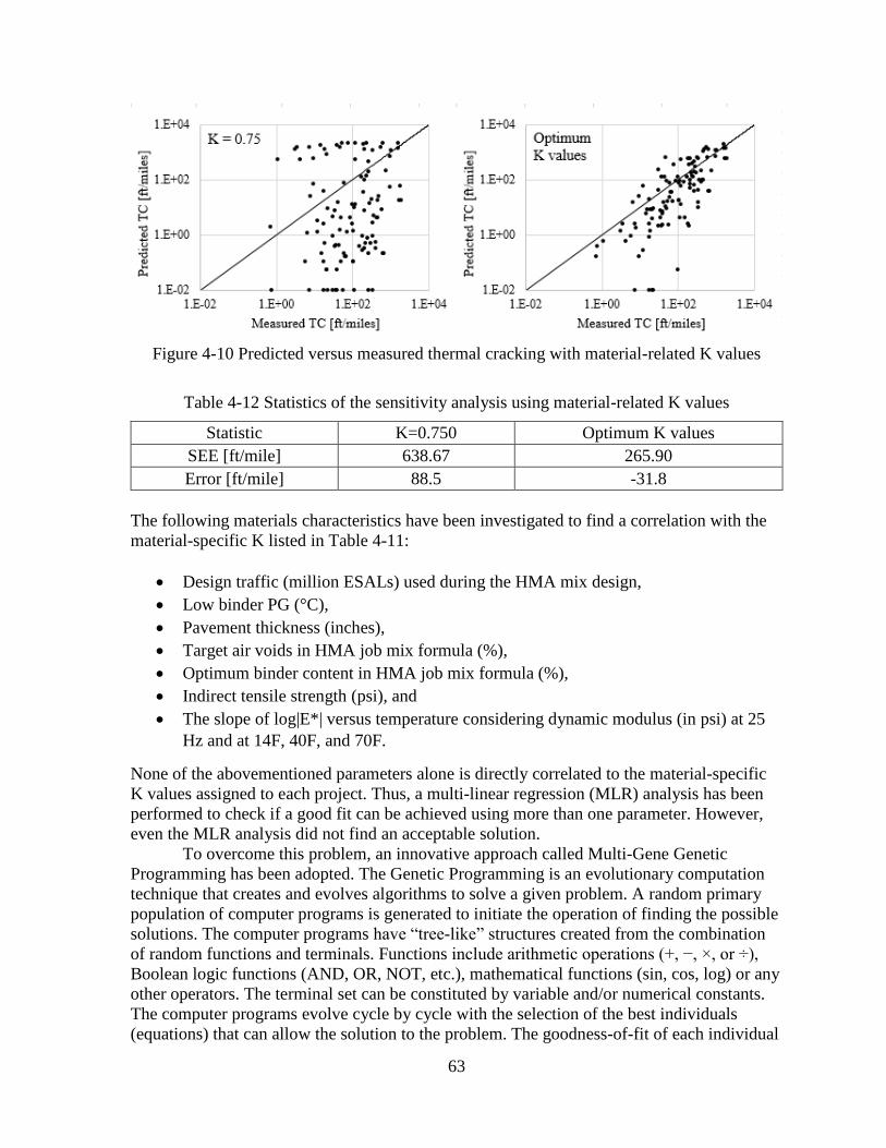
63
Figure 4-10 Predicted versus measured thermal cracking with material-related K values
Table 4-12 Statistics of the sensitivity analysis using material-related K values
Statistic K=0.750 Optimum K values
SEE [ft/mile] 638.67 265.90
Error [ft/mile] 88.5 -31.8
The following materials characteristics have been investigated to find a correlation with the
material-specific K listed in Table 4-11:
Design traffic (million ESALs) used during the HMA mix design,
Low binder PG (°C),
Pavement thickness (inches),
Target air voids in HMA job mix formula (%),
Optimum binder content in HMA job mix formula (%),
Indirect tensile strength (psi), and
The slope of log|E*| versus temperature considering dynamic modulus (in psi) at 25
Hz and at 14F, 40F, and 70F.
None of the abovementioned parameters alone is directly correlated to the material-specific
K values assigned to each project. Thus, a multi-linear regression (MLR) analysis has been
performed to check if a good fit can be achieved using more than one parameter. However,
even the MLR analysis did not find an acceptable solution.
To overcome this problem, an innovative approach called Multi-Gene Genetic
Programming has been adopted. The Genetic Programming is an evolutionary computation
technique that creates and evolves algorithms to solve a given problem. A random primary
population of computer programs is generated to initiate the operation of finding the possible
solutions. The computer programs have “tree-like” structures created from the combination
of random functions and terminals. Functions include arithmetic operations (+, −, ×, or ÷),
Boolean logic functions (AND, OR, NOT, etc.), mathematical functions (sin, cos, log) or any
other operators. The terminal set can be constituted by variable and/or numerical constants.
The computer programs evolve cycle by cycle with the selection of the best individuals
(equations) that can allow the solution to the problem. The goodness-of-fit of each individual
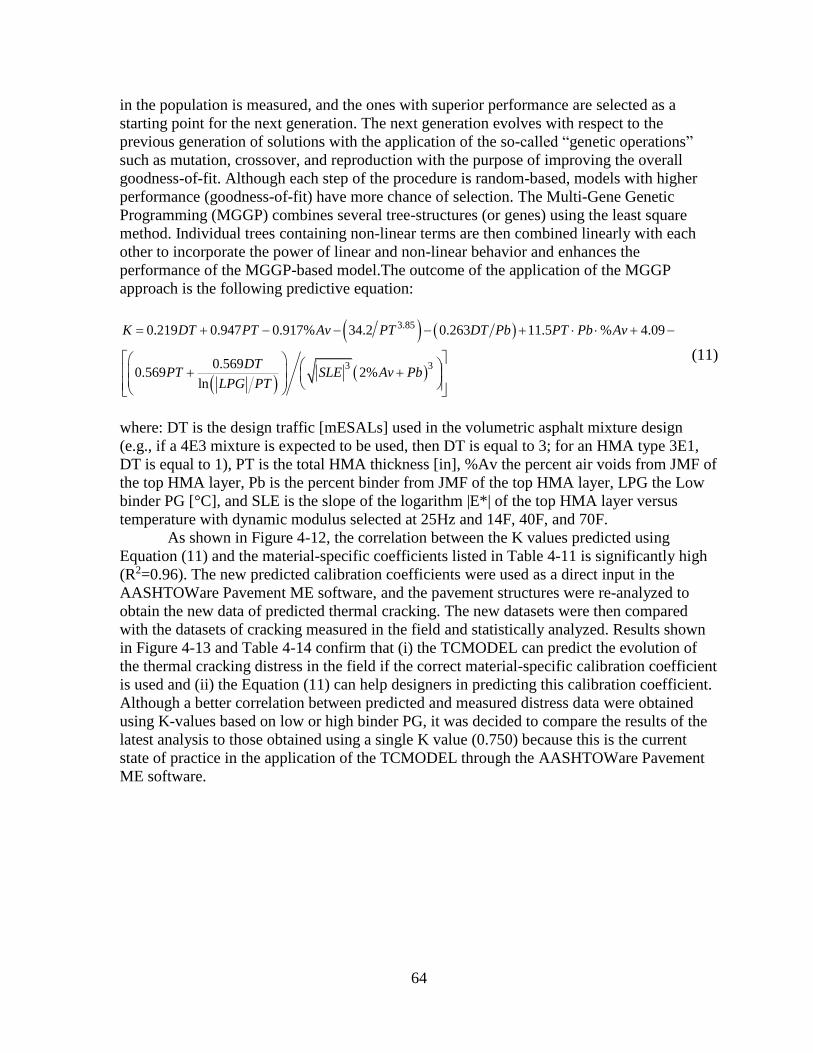
64
in the population is measured, and the ones with superior performance are selected as a
starting point for the next generation. The next generation evolves with respect to the
previous generation of solutions with the application of the so-called “genetic operations”
such as mutation, crossover, and reproduction with the purpose of improving the overall
goodness-of-fit. Although each step of the procedure is random-based, models with higher
performance (goodness-of-fit) have more chance of selection. The Multi-Gene Genetic
Programming (MGGP) combines several tree-structures (or genes) using the least square
method. Individual trees containing non-linear terms are then combined linearly with each
other to incorporate the power of linear and non-linear behavior and enhances the
performance of the MGGP-based model.The outcome of the application of the MGGP
approach is the following predictive equation:
3.85
3 3
0.219 0.947 0.917% 34.2 0.263 11.5 % 4.09
0.5690.569 2%
ln
K DT PT Av PT DT Pb PT Pb Av
DTPT SLE Av Pb
LPG PT
(11)
where: DT is the design traffic [mESALs] used in the volumetric asphalt mixture design
(e.g., if a 4E3 mixture is expected to be used, then DT is equal to 3; for an HMA type 3E1,
DT is equal to 1), PT is the total HMA thickness [in], %Av the percent air voids from JMF of
the top HMA layer, Pb is the percent binder from JMF of the top HMA layer, LPG the Low
binder PG [°C], and SLE is the slope of the logarithm |E*| of the top HMA layer versus
temperature with dynamic modulus selected at 25Hz and 14F, 40F, and 70F.
As shown in Figure 4-12, the correlation between the K values predicted using
Equation (11) and the material-specific coefficients listed in Table 4-11 is significantly high
(R2=0.96). The new predicted calibration coefficients were used as a direct input in the
AASHTOWare Pavement ME software, and the pavement structures were re-analyzed to
obtain the new data of predicted thermal cracking. The new datasets were then compared
with the datasets of cracking measured in the field and statistically analyzed. Results shown
in Figure 4-13 and Table 4-14 confirm that (i) the TCMODEL can predict the evolution of
the thermal cracking distress in the field if the correct material-specific calibration coefficient
is used and (ii) the Equation (11) can help designers in predicting this calibration coefficient.
Although a better correlation between predicted and measured distress data were obtained
using K-values based on low or high binder PG, it was decided to compare the results of the
latest analysis to those obtained using a single K value (0.750) because this is the current
state of practice in the application of the TCMODEL through the AASHTOWare Pavement
ME software.
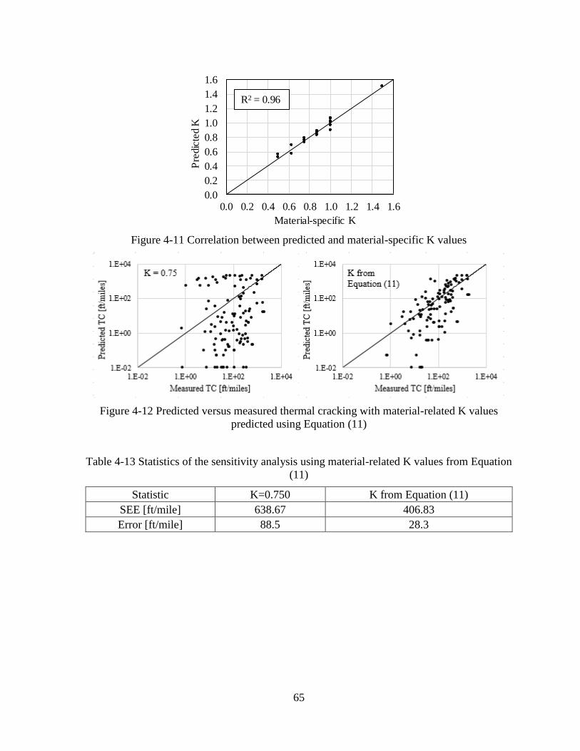
65
Figure 4-11 Correlation between predicted and material-specific K values
Figure 4-12 Predicted versus measured thermal cracking with material-related K values
predicted using Equation (11)
Table 4-13 Statistics of the sensitivity analysis using material-related K values from Equation
(11)
Statistic K=0.750 K from Equation (11)
SEE [ft/mile] 638.67 406.83
Error [ft/mile] 88.5 28.3
0.0
0.2
0.4
0.6
0.8
1.0
1.2
1.4
1.6
0.0 0.2 0.4 0.6 0.8 1.0 1.2 1.4 1.6P
redic
ted K
Material-specific K
R2 = 0.96
66
CHAPTER 5 - CONCLUSIONS AND RECOMMENDATIONS
5.1 SUMMARY
The previous local calibration of the performance models was performed by using version
2.0 of the Pavement-ME software. However, AASHTO has released versions 2.2 and 2.3 of
the software since the completion of the last study. In the revised versions of the software,
several bugs were fixed. Consequently, some of the performance models were modified in
the newer software versions. As a result, the concrete pavement IRI predictions have been
impacted and have raised some concern regarding the resulting PCC slab thicknesses. For
example, for some JPCP pavements in Michigan, the slab thicknesses decreased significantly
by using the same local calibration coefficients between versions 2.0 and 2.2. Consequently,
MDOT decided to use AASHTO 1993 thickness design in the interim since version 2.2 may
provide under designed pavements with calibration coefficients from 2014 study. Because
version 2.2 of the Pavement-ME corrected several coding errors in the software that resulted
in the incorrect calculation of rigid pavements IRI, it was deemed inappropriate to use
version 2.0. Also, concerns about over-predictions and extreme sensitivity in the HMA
thermal cracking model has been observed in some cases. Thus there is also need to evaluate
the use of the thermal cracking model for pavement design in the state of Michigan.
Therefore, the primary objectives of this research project were to (a) evaluate the
differences in JPCP performance models among Pavement-ME versions 2.0. 2.2 and 2.3, (b)
determine the viability of using version 2.0 with current local calibration values, (c)
determine the need for re-calibration of the JPCP performance models, (d) perform local re-
calibration of the JPCP performance models (if warranted) in version 2.2 or 2.3 based on the
identified pavement sections in Michigan, and (e) assess the viability of using the HMA
thermal cracking model for design decisions.
The results showed performance models for rigid pavements (transverse cracking and
IRI) have changed since the Pavement-ME version 2.0. Because of these changes, and
additional time series data being available, re-calibration of the models is warranted and
hence was performed. The local re-calibration of rigid pavement performance models
showed no predicted cracking mainly because the inputs used for design are different from
those used for re-calibration. For example, a compressive strength of 5600 psi is used in
design while an average value of '7.5 cMOR f was used in the initial re-calibration. As a
consequence, the performance models were re-calibrated using as-constructed compressive
strength (values obtained from test results found in the project records) instead of MOR.
Since there was no predicted cracking using a permanent curl of -10oF (default value), the
curl value was varied to match the measured performance for each pavement section in the
calibration dataset. Climate data, material properties, and design parameters were used to
develop a model for predicting permanent curl for each location. This model can be used at
the design stage to estimate permanent curl for a given location in Michigan. The local
calibration coefficients for rigid performance models are documented in the report. For
flexible pavements, the previous local calibration coefficients can still be used because the
prediction models are not modified since the Pavement-ME version 2.0.
67
This research study also investigated the reasons behind the extreme sensitivity of the HMA
thermal cracking model implemented in the Pavement-ME to the properties of asphalt
binders (e.g., Performance Grade) and mixtures (e.g., Indirect Tensile Strength) commonly
employed in Michigan. The thermal cracking model was evaluated to see whether the
extreme sensitivity is due to the model itself or the local calibration coefficient selected in the
previous study. As a result of the investigation, the original local calibration has been re-
assessed by using mix-specific coefficients.
5.2 CONCLUSIONS
Based on the results of the analyses performed, various conclusions were drawn. These
conclusions are listed below:
1. Performance models for rigid pavements (transverse cracking and IRI) have changed
since the Pavement-ME version 2.0. Because of these changes, and additional time series
data being available, re-calibration of the models is warranted.
2. For flexible pavement, the previous local calibration coefficients can still be used because
the prediction models are not modified since the Pavement-ME version 2.0.
3. To predict transverse cracking in rigid pavements with the current design requirements of
MDOT, the permanent curl/warp values should be changed based on the project location.
4. The SEE and bias for the global models for rigid pavement cracking and IRI models are
much higher as compared to the locally re-calibrated models.
5. The median model coefficients based on bootstrapping should be used since the
distributions of SEE and bias are non-normal. The coefficients also showed much lower
SEE and bias than global coefficients for the cracking model.
6. The previously calibrated local joint faulting model coefficients are still valid based on
lowest SEE and bias and should be used.
7. The average IRI model coefficients using bootstrapping showed significantly lower SEE
and bias as compared to the global coefficients.
The following are the conclusions based on the thermal cracking model evaluation for
flexible pavements:
8. Among other factors, one of the factors affecting the parameter n in the crack growth
equation (i.e., nC A K ) is the low-temperature PG of the binder. In general, as PG
decreases (e.g., from PG58-28 to PG58-34), the n also decreases. Since n is in the power
of stress intensity factor (ΔK), small changes in n effect the thermal crack growth (ΔC)
significantly. It was observed that extreme sensitivity of TCMODEL to low PG is
because of this parameter n. For a given K, when PG decreases by one grade, ΔC
decreases by 90-100%. However, when a mix specific K is used, ΔC decreases to a lesser
extent, which is more logical.
9. The literature review on the local calibration of the thermal cracking model in other
States and the analysis of the results obtained in the previous calibration process of the
thermal cracking model for Michigan conditions and materials clearly indicated that:
a. Due to the extreme sensitivity of the model to the mechanical properties of the mixes,
analysis Level 2 and Level 3 must be avoided in the pavement design process,
68
especially for those regions with a cold climate and/or significant thermal
fluctuations. A library of material properties has been created for the Michigan
Department of Transportation, thus it is highly recommended to perform pavement
design only at Level 1.
b. The use of a single local calibration coefficient for entire Michigan ignores the
mixture-to-mixture variability at the local scale. The assignment of mix-specific K-
values is the only solution to predict the thermal cracking accurately.
10. Improvements in thermal cracking prediction have been observed by assigning different
K-values based on the performance grade of the asphalt binders (low or high). However,
the grouping of K based on binder performance grade provides only a marginal
improvement in thermal cracking predictions.
11. Since the behavior of a given mix under the stresses generated by a thermal cycle is
dependent on mix composition and volumetric, the mix-specific coefficients must be a
function of these properties. Thus, each material will have its unique calibration
coefficient (K). The predictive equation developed through the Multi-Gene Genetic
Programming approach allows the designers to assign a calibration coefficient to each
asphalt mixture based on: mix design traffic, total HMA thickness, percent air voids from
JMF of the top HMA layer, percent binder from JMF of the top HMA layer, low binder
PG, and the slope of the logarithm of |E*| of the top HMA layer versus temperature
(dynamic modulus selected at 25Hz and 14F, 40F, and 70F). Correlation between the K
values predicted by the model and the material-specific coefficient found with the
Pavement ME analyses is significantly high (R2=0.96). The comparison between thermal
cracking measured in the field and thermal cracking predicted using mix-specific
coefficients confirm that the thermal cracking model can predict the evolution of the
thermal cracking distress infield if the correct calibration coefficient is used.
5.3 RECOMMENDATIONS
The following are the recommendations based on the findings of this study:
1. The local calibration model coefficients shown in Tables 5-1 and 5-2 can be used to
replace the previous local model's coefficients in Michigan if negligible cracking
predictions are acceptable for rigid pavement designs.
2. The local calibration model coefficients shown in Tables 5-3 and 5-4 can be used to
replace the previous local model's coefficients in Michigan if cracking predictions are
critical for rigid pavement designs.
3. The significant input variables that are related to the various reconstruct and
rehabilitation should be an integral part of a database for construction and material
related information. Such information will be beneficial for future design projects and
local calibration of the performance models in the Pavement-ME.
The following are the recommendations based on thermal cracking model evaluation for
flexible pavements:

69
4. It is recommended to use the TCMODEL implemented in the AASHTO Pavement
ME software to predict thermal cracking distress for flexible pavement design. It is
further recommended that the model coefficient ‘K’ be treated as a mix-specific input
to be able to predict the field behavior accurately.
5. It is recommended to analyze data from additional projects (only 25 sections from the
initial calibration dataset were used) to find the mix-specific calibration coefficients
and develop a new equation based on a more comprehensive set of data. The
additional pavement sections from the initial calibration dataset can be used for this
purpose.
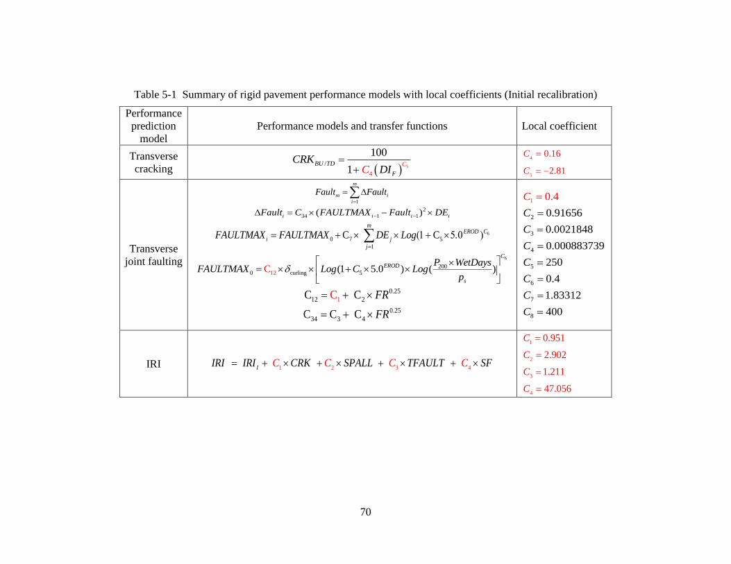
70
Table 5-1 Summary of rigid pavement performance models with local coefficients (Initial recalibration)
Performance
prediction
model
Performance models and transfer functions Local coefficient
Transverse
cracking 5/
4
100
1BU D CT
FCCRK
DI
4
5
0.16
2.81
C
C
Transverse
joint faulting
1
m
m i
i
Fault Fault
2
34 1 1( )i i i iFault C FAULTMAX Fault DE
6
0 7 5
1
C Cm
CEROD
i j
j
FAULTMAX FAULTMAX DE Log
6
2000 curli 512 ng (1 5.0 ) (C )
C
EROD
s
P WetDaysFAULTMAX Log C Log
p
1
0.25
12 2C CC FR
0.25
34 3 4C C C FR
2
3
1
4
5
6
7
8
0.91656
0.0021848
0.000
0.
883739
250
0.4
1.83312
4
4
00
C
C
C
C
C
C
C
C
IRI 1 2 3 4
IIRI IRI CRK SPALL TFAULTC SC FC C
1
2
3
4
0.951
2.902
1.211
47.056
C
C
C
C

71
Table 5-2 Summary of rigid pavement performance model coefficients and standard errors (Initial recalibration)
Performance
prediction
model
Local coefficient Reliability
Transverse
cracking
4
5
0.16
2.81
C
C
0 29463 794
.
e( CRK )s . CRK
Transverse
joint faulting
2
3
1
4
5
6
7
8
0.91656
0.0021848
0.000
0.
883739
250
0.4
1.83312
4
4
00
C
C
C
C
C
C
C
C
0 2698
0 0442.
e( Fault )s . Fault
IRI
1
2
3
4
0.951
2.902
1.211
47.056
C
C
C
C
Internally determined by the
software
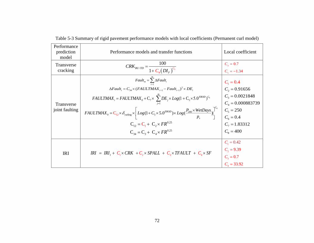
72
Table 5-3 Summary of rigid pavement performance models with local coefficients (Permanent curl model)
Performance
prediction
model
Performance models and transfer functions Local coefficient
Transverse
cracking 5/
4
100
1BU D CT
FCCRK
DI
4
5
0.7
1.34
C
C
Transverse
joint faulting
1
m
m i
i
Fault Fault
2
34 1 1( )i i i iFault C FAULTMAX Fault DE
6
0 7 5
1
C Cm
CEROD
i j
j
FAULTMAX FAULTMAX DE Log
6
2000 curli 512 ng (1 5.0 ) (C )
C
EROD
s
P WetDaysFAULTMAX Log C Log
p
1
0.25
12 2C CC FR
0.25
34 3 4C C C FR
2
3
1
4
5
6
7
8
0.91656
0.0021848
0.000
0.
883739
250
0.4
1.83312
4
4
00
C
C
C
C
C
C
C
C
IRI 1 2 3 4
IIRI IRI CRK SPALL TFAULTC SC FC C
1
2
3
4
0.42
9.39
0.7
33.92
C
C
C
C
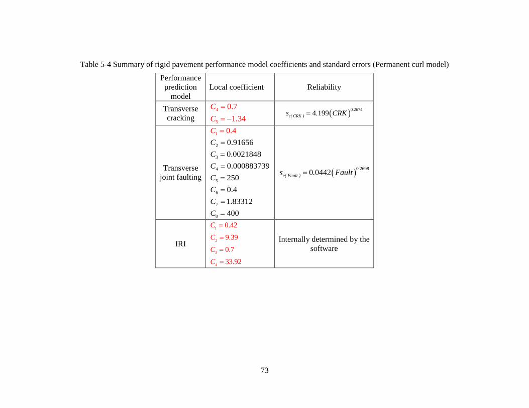
73
Table 5-4 Summary of rigid pavement performance model coefficients and standard errors (Permanent curl model)
Performance
prediction
model
Local coefficient Reliability
Transverse
cracking
4
5
0.7
1.34
C
C
0 26744 199
.
e( CRK )s . CRK
Transverse
joint faulting
2
3
1
4
5
6
7
8
0.91656
0.0021848
0.000
0.
883739
250
0.4
1.83312
4
4
00
C
C
C
C
C
C
C
C
0 2698
0 0442.
e( Fault )s . Fault
IRI
1
2
3
4
0.42
9.39
0.7
33.92
C
C
C
C
Internally determined by the
software
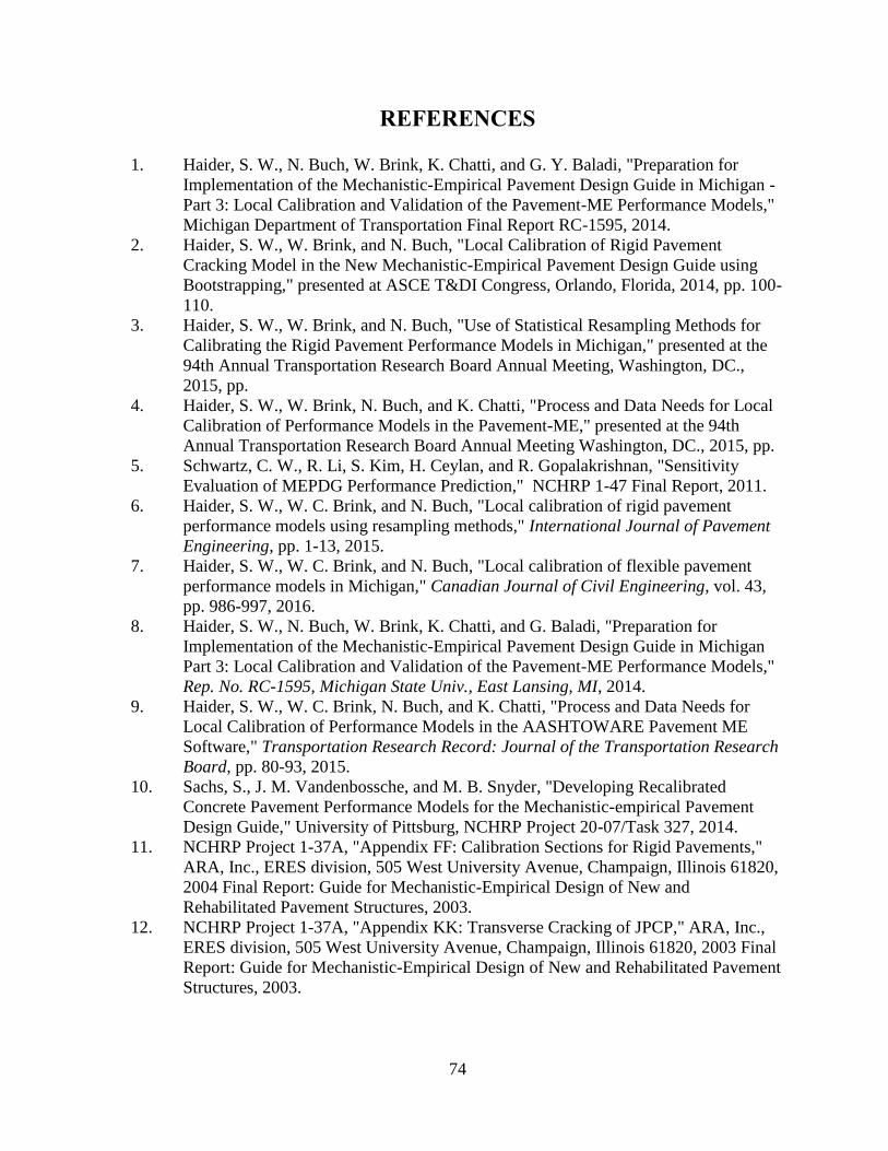
74
REFERENCES 1. Haider, S. W., N. Buch, W. Brink, K. Chatti, and G. Y. Baladi, "Preparation for
Implementation of the Mechanistic-Empirical Pavement Design Guide in Michigan -
Part 3: Local Calibration and Validation of the Pavement-ME Performance Models,"
Michigan Department of Transportation Final Report RC-1595, 2014.
2. Haider, S. W., W. Brink, and N. Buch, "Local Calibration of Rigid Pavement
Cracking Model in the New Mechanistic-Empirical Pavement Design Guide using
Bootstrapping," presented at ASCE T&DI Congress, Orlando, Florida, 2014, pp. 100-
110.
3. Haider, S. W., W. Brink, and N. Buch, "Use of Statistical Resampling Methods for
Calibrating the Rigid Pavement Performance Models in Michigan," presented at the
94th Annual Transportation Research Board Annual Meeting, Washington, DC.,
2015, pp.
4. Haider, S. W., W. Brink, N. Buch, and K. Chatti, "Process and Data Needs for Local
Calibration of Performance Models in the Pavement-ME," presented at the 94th
Annual Transportation Research Board Annual Meeting Washington, DC., 2015, pp.
5. Schwartz, C. W., R. Li, S. Kim, H. Ceylan, and R. Gopalakrishnan, "Sensitivity
Evaluation of MEPDG Performance Prediction," NCHRP 1-47 Final Report, 2011.
6. Haider, S. W., W. C. Brink, and N. Buch, "Local calibration of rigid pavement
performance models using resampling methods," International Journal of Pavement
Engineering, pp. 1-13, 2015.
7. Haider, S. W., W. C. Brink, and N. Buch, "Local calibration of flexible pavement
performance models in Michigan," Canadian Journal of Civil Engineering, vol. 43,
pp. 986-997, 2016.
8. Haider, S. W., N. Buch, W. Brink, K. Chatti, and G. Baladi, "Preparation for
Implementation of the Mechanistic-Empirical Pavement Design Guide in Michigan
Part 3: Local Calibration and Validation of the Pavement-ME Performance Models,"
Rep. No. RC-1595, Michigan State Univ., East Lansing, MI, 2014.
9. Haider, S. W., W. C. Brink, N. Buch, and K. Chatti, "Process and Data Needs for
Local Calibration of Performance Models in the AASHTOWARE Pavement ME
Software," Transportation Research Record: Journal of the Transportation Research
Board, pp. 80-93, 2015.
10. Sachs, S., J. M. Vandenbossche, and M. B. Snyder, "Developing Recalibrated
Concrete Pavement Performance Models for the Mechanistic-empirical Pavement
Design Guide," University of Pittsburg, NCHRP Project 20-07/Task 327, 2014.
11. NCHRP Project 1-37A, "Appendix FF: Calibration Sections for Rigid Pavements,"
ARA, Inc., ERES division, 505 West University Avenue, Champaign, Illinois 61820,
2004 Final Report: Guide for Mechanistic-Empirical Design of New and
Rehabilitated Pavement Structures, 2003.
12. NCHRP Project 1-37A, "Appendix KK: Transverse Cracking of JPCP," ARA, Inc.,
ERES division, 505 West University Avenue, Champaign, Illinois 61820, 2003 Final
Report: Guide for Mechanistic-Empirical Design of New and Rehabilitated Pavement
Structures, 2003.

75
13. Rao, C., L. Titus-Glover, B. Bhattacharya, M. Darter, M. Stanley, and H. Von
Quintus, "Estimation of Key PCC, Base, Subbase, and Pavement Engineering
Properties from Routine Tests and Physical Characteristics," 2012.
14. Finn, F., C. L. Saraf, R. Kulkarni, K. Nair, W. Smith, and A. Abdullah, "NCHRP
Report 291 - Development of pavement structural subsystems," 1986.
15. Fromm, H. J., and W. A. Phang, "A Study of Transverse Cracking of Bituminous
Pavements," presented at Proceedings of the Association of Asphalt Paving
Technologists, 1972, pp. 383-418.
16. Haas, R., F. Meyer, G. Assaf, and H. Lee, "A comprehensive study of cold climate
airport pavement cracking," presented at Proceedings of the Association of Asphalt
Paving Technologists, 1987, pp. 198-245.
17. Roque, R. and B. E. Ruth, "Mechanisms and modeling of surface cracking in asphalt
pavements," Journal of the Association of Asphalt Paving Technologists, vol. 59, pp.
396-421, 1990.
18. Paris, P. C., M. P. Gomez, and W. E. Anderson, "A rational analytical theory of
fatigue," The Trend in Engineering, vol. 13, 1961.
19. Schapery, R. A., "A theory of crack growth in viscoelastic media," 1973.
20. Molenaar, A. A. A., "Fatigue and reflection cracking due to traffic loads," presented
at Proceedings of the Association of Asphalt Paving Technologists, 1984, pp. 440-
474.
21. Lytton, R., U. Shanmugham, and B. D. Garrett, "Design of asphalt pavements for
thermal fatigue cracking," 1983.
22. Haider, S. W., N. Buch, W. Brink, K. Chatti, and G. Baladi, "Preparation for
Implementation of the Mechanistic-Empirical Pavement Design Guide in Michigan
Part 3: Local Calibration and Validation of the Pavement - ME Performance Models
Final Report," 2014.
23. Pierce, L. M., and G. McGovern, "NCHRP Synthesis 457 - Implementation of the
AASHTO Mechanistic-Empirical Pavement Design Guide and Software," 2014.
24. Ceylan, H., K. Sunghwan, G. Kasthurirangan, and M. Di, "Iowa Calibration of
MEPDG Performance Prediction Models," 2013.
25. Hall, K. D., D. Xiao, and K. Wang, "Calibration of the MEPDG for Flexible
Pavement Design in Arkansas," presented at Proceedings of the 2011 Annual Meeting
of the Transportation Research Board, 2011, pp.
26. Velasquez, R., K. Hoegh, I. Yut, M. Funk, G. Cochran, M. Marasteanu, and L.
Khazanovich, "Implementation of the MEPDG for New and Rehabilitated Pavement
Structures for Design of Concrete and Asphalt Pavements in Minnesota," 2009.
27. Marasteanu, M., W. Buttlar, H. Bahia, and C. Williams, "Investigation of Low
Temperature Cracking in Asphalt Pavements National Pooled Fund Study - Phase II,"
2012.
28. von Quintus, H. and J. Moulthrop, "Mechanistic-Empirical Pavement Design Guide
Flexible Pavement Performance Prediction Models for Montana: Volume I Executive
Research Summary," 2007.
29. Glover, L. and J. Mallela, "Guidelines for Implementing NCHRP 1-37A M-E Design
Procedures in Ohio : Volume 4 - MEPDG Models Validation & Recalibration,"
2009.

76
30. Hoerner, T., K. Zimmerman, K. Smith, and L. Cooley, "Mechanistic-Empirical
Pavement Design Guide Implementation Plan," 2007.
31. Bhattacharya, B., H. von Quintus, and M. Darter, "Implementation and local
calibration of the MEPDG transfer functions in Wyoming," 2015.
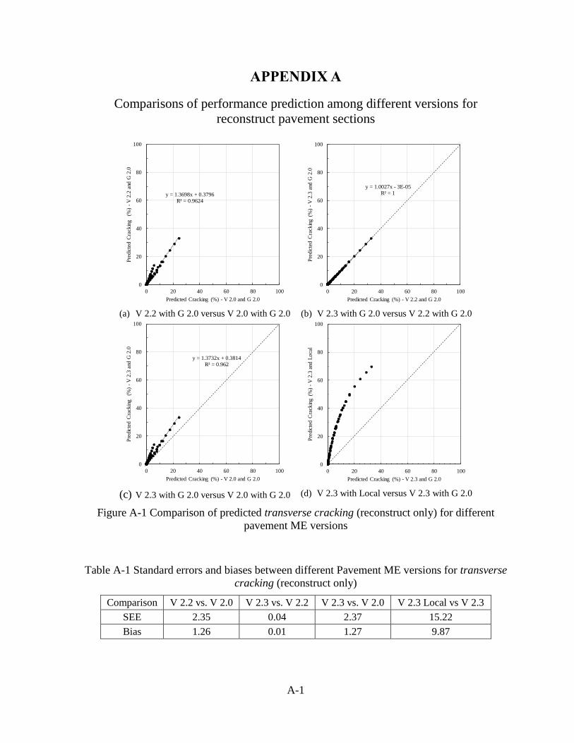
A-1
APPENDIX A
Comparisons of performance prediction among different versions for
reconstruct pavement sections
(a) V 2.2 with G 2.0 versus V 2.0 with G 2.0
(b) V 2.3 with G 2.0 versus V 2.2 with G 2.0
(c) V 2.3 with G 2.0 versus V 2.0 with G 2.0
(d) V 2.3 with Local versus V 2.3 with G 2.0
Figure A-1 Comparison of predicted transverse cracking (reconstruct only) for different
pavement ME versions
Table A-1 Standard errors and biases between different Pavement ME versions for transverse
cracking (reconstruct only)
Comparison V 2.2 vs. V 2.0 V 2.3 vs. V 2.2 V 2.3 vs. V 2.0 V 2.3 Local vs V 2.3
SEE 2.35 0.04 2.37 15.22
Bias 1.26 0.01 1.27 9.87
y = 1.3698x + 0.3796R² = 0.9624
0
20
40
60
80
100
0 20 40 60 80 100
Pre
dic
ted C
rack
ing
(%)
-V
2.2
and
G 2
.0
Predicted Cracking (%) - V 2.0 and G 2.0
y = 1.0027x - 3E-05R² = 1
0
20
40
60
80
100
0 20 40 60 80 100
Pre
dic
ted
Cra
ckin
g(%
) -
V 2
.3 a
nd G
2.0
Predicted Cracking (%) - V 2.2 and G 2.0
y = 1.3732x + 0.3814R² = 0.962
0
20
40
60
80
100
0 20 40 60 80 100
Pre
dic
ted C
rack
ing
(%)
-V
2.3
and
G 2
.0
Predicted Cracking (%) - V 2.0 and G 2.0
0
20
40
60
80
100
0 20 40 60 80 100
Pre
dic
ted C
rack
ing
(%)
-V
2.3
and
Loca
l
Predicted Cracking (%) - V 2.3 and G 2.0
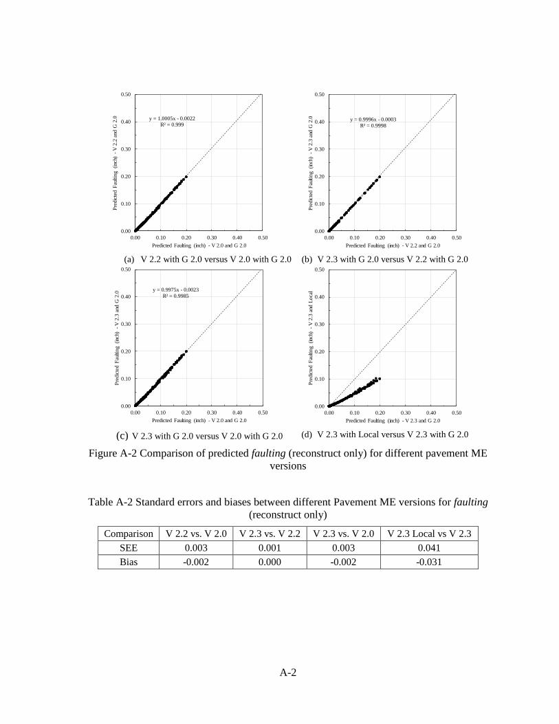
A-2
(a) V 2.2 with G 2.0 versus V 2.0 with G 2.0
(b) V 2.3 with G 2.0 versus V 2.2 with G 2.0
(c) V 2.3 with G 2.0 versus V 2.0 with G 2.0
(d) V 2.3 with Local versus V 2.3 with G 2.0
Figure A-2 Comparison of predicted faulting (reconstruct only) for different pavement ME
versions
Table A-2 Standard errors and biases between different Pavement ME versions for faulting
(reconstruct only)
Comparison V 2.2 vs. V 2.0 V 2.3 vs. V 2.2 V 2.3 vs. V 2.0 V 2.3 Local vs V 2.3
SEE 0.003 0.001 0.003 0.041
Bias -0.002 0.000 -0.002 -0.031
y = 1.0005x - 0.0022R² = 0.999
0.00
0.10
0.20
0.30
0.40
0.50
0.00 0.10 0.20 0.30 0.40 0.50
Pre
dic
ted F
aulti
ng
(inc
h) -
V 2
.2 a
nd G
2.0
Predicted Faulting (inch) - V 2.0 and G 2.0
y = 0.9996x - 0.0003R² = 0.9998
0.00
0.10
0.20
0.30
0.40
0.50
0.00 0.10 0.20 0.30 0.40 0.50
Pre
dic
ted F
aulti
ng
(inc
h)
-V
2.3
and
G 2
.0
Predicted Faulting (inch) - V 2.2 and G 2.0
y = 0.9975x - 0.0023R² = 0.9985
0.00
0.10
0.20
0.30
0.40
0.50
0.00 0.10 0.20 0.30 0.40 0.50
Pre
dic
ted F
aulti
ng
(inc
h)
-V
2.3
and
G 2
.0
Predicted Faulting (inch) - V 2.0 and G 2.0
0.00
0.10
0.20
0.30
0.40
0.50
0.00 0.10 0.20 0.30 0.40 0.50
Pre
dic
ted F
aulti
ng
(inc
h)
-V
2.3
and
Loca
l
Predicted Faulting (inch) - V 2.3 and G 2.0
A-3
(a) V 2.2 with G 2.0 versus V 2.0 with G 2.0
(b) V 2.3 with G 2.0 versus V 2.2 with G 2.0
(c) V 2.3 with G 2.0 versus V 2.0 with G 2.0
(d) V 2.3 with Local versus V 2.3 with G 2.0
Figure A-3 Comparison of predicted IRI (reconstruct only) for different pavement ME
versions
Table A-3 Standard errors and biases between different Pavement ME versions for IRI
(reconstruct)
Comparison V 2.2 vs. V 2.0 V 2.3 vs. V 2.2 V 2.3 vs. V 2.0 V 2.3 Local vs V 2.3
SEE 5.96 0.65 5.99 17.48
Bias -4.2 -0.1 -4.3 2.7
y = 0.9708x - 0.9724R² = 0.98
0
50
100
150
200
250
300
0 50 100 150 200 250 300
Pre
dic
ted
IR
I (i
nch/
mil
e)
-V
2.2
and
G 2
.0
Predicted IRI (inch/mile) - V 2.0 and G 2.0
y = 0.9996x - 0.0721R² = 0.9995
0
50
100
150
200
250
300
0 50 100 150 200 250 300
Pre
dic
ted
IR
I (inc
h/m
ile)
-
V 2
.3 a
nd G
2.0
Predicted IRI (inch/mile) - V 2.2 and G 2.0
y = 0.971x - 1.1091R² = 0.9807
0
50
100
150
200
250
300
0 50 100 150 200 250 300
Pre
dic
ted
IR
I (inc
h/m
ile)
-
V 2
.3 a
nd G
2.0
Predicted IRI (inch/mile) - V 2.0 and G 2.0
0
50
100
150
200
250
300
0 50 100 150 200 250 300
Pre
dic
ted
IR
I (inc
h/m
ile)
-
V 2
.3 a
nd L
oca
l
Predicted IRI (inch/mile) - V 2.3 and G 2.0
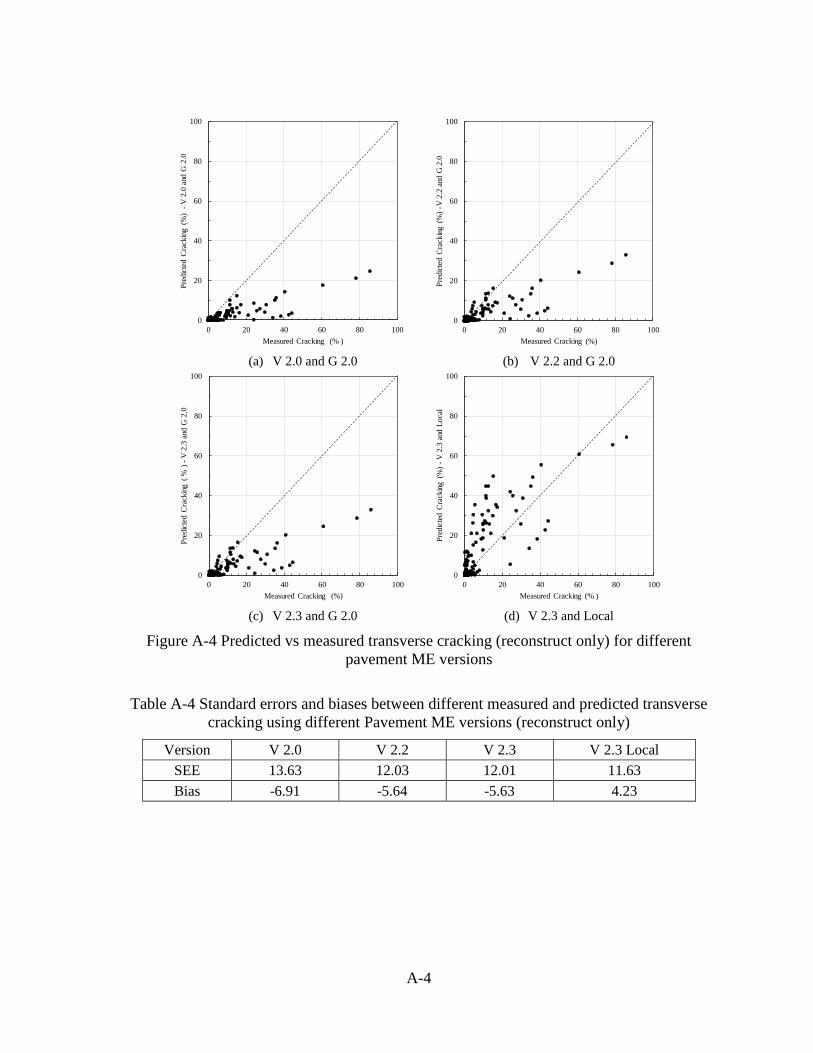
A-4
(a) V 2.0 and G 2.0
(b) V 2.2 and G 2.0
(c) V 2.3 and G 2.0
(d) V 2.3 and Local
Figure A-4 Predicted vs measured transverse cracking (reconstruct only) for different
pavement ME versions
Table A-4 Standard errors and biases between different measured and predicted transverse
cracking using different Pavement ME versions (reconstruct only)
Version V 2.0 V 2.2 V 2.3 V 2.3 Local
SEE 13.63 12.03 12.01 11.63
Bias -6.91 -5.64 -5.63 4.23
0
20
40
60
80
100
0 20 40 60 80 100
Pre
dic
ted C
rack
ing
(%)
-V
2.0
and
G 2
.0
Measured Cracking (% )
0
20
40
60
80
100
0 20 40 60 80 100
Pre
dic
ted C
rack
ing
(%)
-V 2
.2 a
nd G
2.0
Measured Cracking (%)
0
20
40
60
80
100
0 20 40 60 80 100
Pre
dic
ted
Cra
ckin
g(
%)
-V
2.3
and
G 2
.0
Measured Cracking (%)
0
20
40
60
80
100
0 20 40 60 80 100
Pre
dic
ted
Cra
ckin
g(%
) -
V 2
.3 a
nd L
oca
l
Measured Cracking (% )
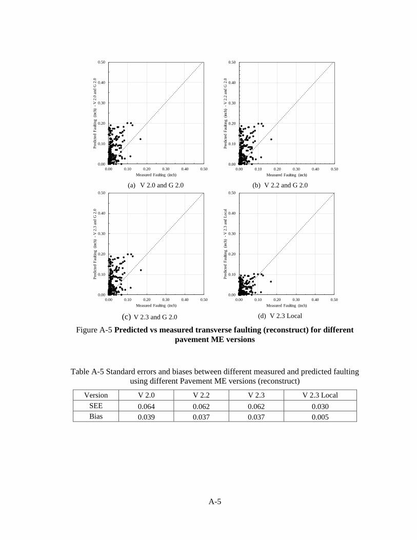
A-5
(a) V 2.0 and G 2.0
(b) V 2.2 and G 2.0
(c) V 2.3 and G 2.0
(d) V 2.3 Local
Figure A-5 Predicted vs measured transverse faulting (reconstruct) for different
pavement ME versions
Table A-5 Standard errors and biases between different measured and predicted faulting
using different Pavement ME versions (reconstruct)
Version V 2.0 V 2.2 V 2.3 V 2.3 Local
SEE 0.064 0.062 0.062 0.030
Bias 0.039 0.037 0.037 0.005
0.00
0.10
0.20
0.30
0.40
0.50
0.00 0.10 0.20 0.30 0.40 0.50
Pre
dic
ted
Fau
ltin
g (i
nch)
-
V 2
.0 a
nd G
2.0
Measured Faulting (inch)
0.00
0.10
0.20
0.30
0.40
0.50
0.00 0.10 0.20 0.30 0.40 0.50
Pre
dic
ted
Fau
ltin
g (inc
h)
-V
2.2
and
G 2
.0
Measured Faulting (inch)
0.00
0.10
0.20
0.30
0.40
0.50
0.00 0.10 0.20 0.30 0.40 0.50
Pre
dic
ted
Fau
ltin
g (inc
h)
-V
2.3
and
G 2
.0
Measured Faulting (inch)
0.00
0.10
0.20
0.30
0.40
0.50
0.00 0.10 0.20 0.30 0.40 0.50
Pre
dic
ted
Fau
ltin
g (inc
h)
-V
2.3
and
Lo
cal
Measured Faulting (inch)
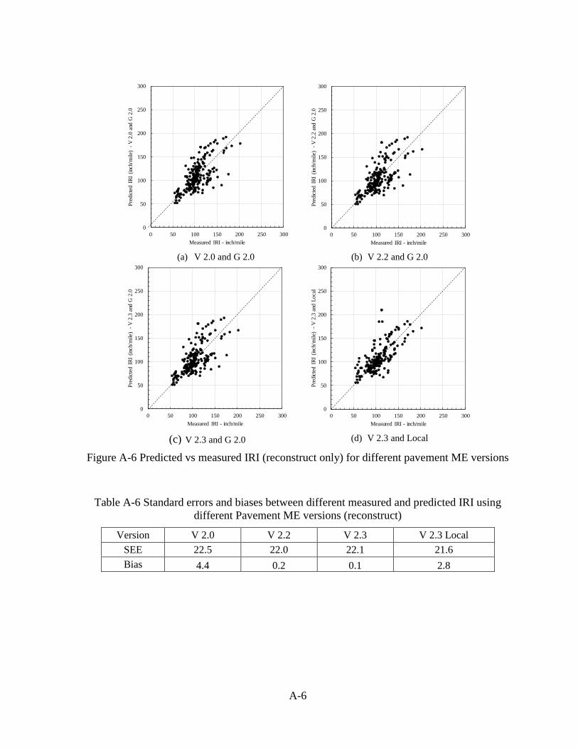
A-6
(a) V 2.0 and G 2.0
(b) V 2.2 and G 2.0
(c) V 2.3 and G 2.0
(d) V 2.3 and Local
Figure A-6 Predicted vs measured IRI (reconstruct only) for different pavement ME versions
Table A-6 Standard errors and biases between different measured and predicted IRI using
different Pavement ME versions (reconstruct)
Version V 2.0 V 2.2 V 2.3 V 2.3 Local
SEE 22.5 22.0 22.1 21.6
Bias 4.4 0.2 0.1 2.8
0
50
100
150
200
250
300
0 50 100 150 200 250 300
Pre
dic
ted
IR
I (i
nch/
mil
e)
-V
2.0
and
G 2
.0
Measured IRI - inch/mile
0
50
100
150
200
250
300
0 50 100 150 200 250 300
Pre
dic
ted
IR
I (inc
h/m
ile)
-
V 2
.2 a
nd G
2.0
Measured IRI - inch/mile
0
50
100
150
200
250
300
0 50 100 150 200 250 300
Pre
dic
ted
IR
I (inc
h/m
ile)
-
V 2
.3 a
nd G
2.0
Measured IRI - inch/mile
0
50
100
150
200
250
300
0 50 100 150 200 250 300
Pre
dic
ted
IR
I (inc
h/m
ile)
-
V 2
.3 a
nd L
oca
l
Measured IRI - inch/mile