How Do Managers Matter? Evidence from PerformanceMetrics and Employee Surveys in a Firm∗

Mitchell Hoffman†

Steven Tadelis‡

April 2017

Abstract

Many companies survey employees about their managers yet it is unclear whetherthis information is, or should be used to evaluate and compensate managers. Data froma high-tech firm reveals that survey measures are associated with employees’ lower attri-tion, higher promotions, higher salary increases, and higher engagement, but have onlya limited relation to subjective performance scores. The strongest results are on attri-tion, and different research designs (exploiting new workers joining the firm or exploitingmanager moves) support a causal relation of survey-based manager quality to employeeattrition. However, managers with better survey scores receive limited benefits in termsof compensation and other rewards.

JEL Classifications : D23, J24, L23, M53Keywords : Management, productivity, supervisors, leadership, employee surveys

∗We thank Heski Bar-Isaac, Jordi Blanes i Vidal, Nick Bloom, Kevin Bryan, Wouter Dessein, MariaGuadalupe, Tom Hubbard, Pat Kline, Harry Krashinsky, Eddie Lazear, Bentley MacLeod, Kathryn Shaw, andnumerous conference/seminar participants for helpful comments. Hoffman acknowledges financial support fromthe Connaught New Researcher Award and the Social Science and Humanities Research Council of Canada.†University of Toronto Rotman School of Management and NBER; mitchell.hoffman@rotman.utoronto.ca‡UC Berkeley Haas School of Business and NBER; stadelis@berkeley.edu

1 Introduction

The relationship between managers and employees is fundamental to the success of firms,

and has recently gained traction in labor and organizational economics research. As scholars

have sought to explore if and how management plays a role in exploring large productivity

differences across firms and countries (Bloom and Van Reenen, 2011; Hsieh and Klenow, 2009;

Syverson, 2004, 2011), increasing attention is being devoted to the managers themselves. It

seems evident that good managers matter. Many people pay handsomely to attend business

school to become better managers, and scores of books are written every year on how to become

a better manager. Unfortunately, little empirical evidence exists regarding the managerial

production function, particularly at the micro level.

What is it that managers do? How much do managers matter? Are good managers

rewarded for their contributions? We seek to answer these and related questions using rich

employee surveys conducted by a multinational technology and services firm. Employees

in our firm are asked to evaluate their managers on a number of dimensions, e.g., whether

they are trustworthy or whether they provide adequate coaching. We are thus able to go

beyond examining whether managers matter, and can identify the particular questions that

best predict some measures of employee outcomes.

Some progress has been made recently in examining how much managers matter using a

“value-added” approach. For example, Bertrand and Schoar (2003) examine how much CEOs

matter for various decisions in firms by regressing various firm outcomes on CEO fixed effects.

Lazear et al. (2015) use data from one firm to examine to what extent low-level managers

(specifically, front-line supervisors) matter for productivity, finding that they matter a great

deal. Hoffman et al. (2015b) use data from several firms to examine the determinants of

low-level manager productivity around the world.1

While these studies are of great interest, the value-added approach faces several limi-

1Bender et al. (2016) analyze interactions between employees/managers and management practices inGermany.

1

tations. First, these studies require good objective data on worker productivity. However,

in many firms, direct data on individual worker productivity is often scarce, and sometimes

impossible to measure, particularly in high-skill collaborative environments. When data are

available, productivity metrics may be subject to various shocks (e.g., business generated by

a law-firm partner could be adversely affected by the exit of a single prominent client, who

decided to leave the firm for reasons having nothing to do with the partner). Second, in

the value-added approach, significant concern is placed on whether the data used are able to

truly isolate the incremental effect of being a better manager, or whether selection issues are

confounding causal impacts. Moreover, the fixed effects do not reveal by themselves why some

managers may be better than others.

We take a different approach. Rather than solely leveraging fixed effects, we take advan-

tage of our rich survey data, combined with a variety of outcome measures we have obtained

from the firm. In particular, we create a measure of “manager quality” using employees’

survey responses about their manager. We then proceed to explore the extent to which these

responses correlate with employee outcomes at the firm. We combine a variety of survey-based

analyses together with a value-added approach so we can compare the survey and value-added

approaches. The data from the firm cover thousands of managers and tens of thousands of

employees. The data contain a large number of knowledge workers, as well as a large number

of lower-skill workers, allowing us to examine heterogeneity in our analysis across many types

of employees and levels in the hierarchy.

Managers are hired to enhance the productivity of their employees and to help them suc-

ceed in their jobs. Asking employees about the extent to which their manager improves their

performance and impacts their success thus seems like a natural way to measure managerial

performance, and is one that has been pursued by many firms.2 Indeed, Brutus et al. (2006)

report that over one third of US and Canadian organizations in their survey reported using

“multi-source assessments” (as opposed to only assessing individuals based on their managers)

2See, for example, the case of Project Oxygen at Google (Garvin et al., 2013) and the case of Royal Bankof Canada (Shaw and Schifrin, 2015).

2

and Pfau et al. (2002) reports that 65% of firms use 360-degree performance evaluation. Our

approach of analyzing managers using employee surveys thus appears to align closely to the

data practices of many firms.

An obvious challenge in using employee surveys is the possibility that employees may

not be truthful. Workers generally care about what their managers think about them, and

may be highly averse to saying something negative about them. This concern is mitigated

in our data due to the confidential nature of the survey. Workers are told truthfully that

their individual responses cannot and will never be observed by the firm. Instead, managers

receive aggregated results, and even that occurs only for managers with a minimum number of

employees responding. Our data is thus limited to manager-year averages for various qualities

ascribed to them by their employees. This feature protects worker confidentiality, but does

not limit our analysis, given our focus on understanding behavior at the manager level.

Our first main finding is that managers matter a lot for some but not all measurable

employee outcomes. Increasing an aggregate measure of manager quality by one standard

deviation is associated with roughly a 12% reduction in employee turnover. This result holds

not only with lower skill employees, but also with engineers, for whom the association is

actually stronger. Manager quality is also associated with employees being more engaged,

but the relation to turnover is only partially driven by the relationship with engagement. We

further find positive correlations between manager quality and employees getting promoted,

as well as between manager quality and employee salary increases. Interestingly, manager

quality does not appear to relate much to subjective performance scores of employees. There

is no single managerial characteristic from the survey that is most important, but rather all

are often present in good managers.

An important question is whether these correlations are causal. The concern is there

could be unobserved shocks or measurement error that could influence both measured manager

quality and employee outcomes. We address this concern using two identification strategies

in the spirit of those in the “teacher fixed effects” literature (Chetty et al., 2014). Our first

3

strategy analyzes outcomes of employees who join mid-way through our sample as a function

of manager quality measured before the employees join the firm. This addresses contempora-

neous shocks affecting manager ratings and employee outcomes. Our second strategy studies

managers moving across work teams and locations within the firm, measuring manager qual-

ity before the move takes place. This strategy addresses more permanent unobserved shocks

(beyond what are already measured using our rich, baseline controls). Both strategies tend

to support that the initial correlations we document are causal, particularly those related to

attrition.

Our second main finding shows that while higher quality managers attain somewhat

higher subjective performance scores, they do not appear to be paid more, nor do they appear

to reap much of other rewards (such as in getting promoted). Manager value-added also does

not appear to be strongly associated with reward. In contrast, a manager’s own subjective

performance score (that is, the rating from his/her higher-ups) is strongly associated with

both pay and other rewards. Unlike subjective performance, our measure of manager quality

does not predict whether a manager becomes more likely to be fired.3 Overall, what the

higher-ups think of a manager appear more important for a manager’s rewards than what the

manager’s direct reports express. An important exception is in span of control, where better

people managers obtain higher spans.

Our paper contributes to several literatures. First, as discussed above, it is related to

work on the importance of individual managers.4 Second, it is related to work on subjective

performance evaluation and workplace feedback. Employee surveys bring to bear an advan-

tage often ascribed to subjective performance evaluation, namely, that they help account for

difficult-to-measure aspects of performance (Baker et al., 1994b). A main contribution of our

paper is bringing forward a new aspect of performance evaluation, namely reports from a

3We use the word “fired” as a shorthand for an involuntary exit. We cannot distinguish a lay-off from aninvoluntary discharge in the data. However, we can distinguish voluntary from involuntary exits.

4Beyond the work cited above, Bandiera et al. (2016) classify CEOs into two types and find that one type(representing a higher tendency to delegate) tends to significantly outperform the other. In a field experiment,Friebel et al. (2016) find that increased communication from upper management to store managers leadsmanagers to reduce turnover.

4

manager’s employees, that has not been previously explored in economics.5

Third, it relates to studies of compensation and reward within organizations (e.g., Baker

et al., 1994a). Fourth, it relates to work in general on knowledge-based employees. Much of

empirical personnel economics focuses on relatively low-skilled jobs (e.g., truckers, retail, and

farm-workers), partially because it is often relatively simple in those jobs to measure individual

productivity. In contrast, for high-skilled jobs for knowledge employees, production is often

complex, multi-faceted, and involves teamwork. Our analysis sheds light on the managerial

production function in such a high-skilled setting.

The paper proceeds as follows. Section 2 describes the data, including what survey data

are available. Section 3 describes our empirical strategy. Section 4 provides our analyses

relating the survey data to employee outcomes. Section 5 analyzes how good managers are

rewarded. Section 6 concludes.

2 Data and Institutional Setting

Our data, obtained from a technology and services company, covers a period of two years

and five months, some time between January 2011 and December 2015. To preserve firm

confidentiality, certain details regarding the firm cannot be provided. We refer to the three

years of the data as Y1, Y2, and Y3. Between January Y1 and May Y3, we observe several

dozen thousands of employees and several hundreds of thousands of employee months. The

data cover several business units.

About 63% of workers are in the US, with the remainder located abroad. An observation

is a worker-month, and about 16% of observations are filled by individuals in managerial roles,

so the majority of observations are for non-managers (often referred to in industry as individual

5In economics, there are papers studying job satisfaction surveys (e.g., Clark, 2001; Frederiksen, forthcom-ing), thereby complementing our work which focuses on managers. In industrial psychology, there is work on360 degree performance evaluation (e.g., Atkins and Wood, 2002). In economics, there is also a parallel withrespect to a literature on student evaluations of teachers (e.g., Beleche et al., 2012). Carrell and West (2010)show that teacher evaluations positively correlate with contemporaneous student value-added, but negativelycorrelate with later achievement.

5

contributors). While our data begin in Jan. Y1, the majority of the workers are hired before

that date. Still, 38% of the employees in the data were hired on or after Jan. Y1. The data

cover workers only, and do not cover applicants.6

The firm is divided into several broad business units. From a functional standpoint,

roughly 32% of worker-months are in customer service/operations and 22% of worker-months

are in engineering, with the remainder in other business functions (e.g., marketing, finance,

sales, etc.). We next provide information on employee outcomes, manager assignment, and

the employee surveys, with further details regarding the data in Appendix B.

2.1 Employee Outcomes

In knowledge-based firms such as the one we study (as well as in non-knowledge-based firms),

employee performance often has multiple dimensions. These are the five core employee out-

comes in our data:

1. Turnover. Employee turnover is a significant issue in many organizations, and in high-

tech organizations in particular, where the knowledge of employees represents a key

asset. We separately observe dates of voluntary quits and involuntary fires.

2. Subjective performance. The firm’s subjective performance scores are set biannually

on a scale from 1 to 5, as in the case in many organizations that use subjective perfor-

mance evaluation (Frederiksen et al., 2014). Subjective performance scores are set in

a process involving an employee’s immediate manager as well as higher-up managers.

While there are some broad guidelines for the distribution of subjective performance

scores across various units within the firm, there is not a fixed “curve” across managers

in the number of subjective performance scores that can be provided.7

6This is in contrast to recent papers such as Burks et al. (2015) and Hoffman et al. (2015a), which alsocover applicants.

7At high levels of aggregation within the organization (that is, for top managers), there may be a curve withrespect to subjective performance. To address this, we can examine the robustness of subjective performanceresults to excluding top managers.

6

3. Employee engagement. Engagement is a number from 0-100 about how engaged the

employee is feeling (via the same survey that is used to elicit information on employees’

view of their manager), which is then normalized. Employee engagement is a variable

that seems to have received limited attention within labor and organizational economics

(Blader et al. (2016) is a recent exception). However, within industrial psychology and

management, employee engagement is an outcome of significant interest (Kahn, 1990).

4. Salary increases. While it is difficult to measure the productivity of knowledge work-

ers, we can attempt to proxy productivity improvements by the extent to which an

employee’s salary increases.

5. Promotions. Another recent paper using promotions as a proxy for knowledge worker

productivity is Brown et al. (2016).

Different employee outcomes are available at different frequencies, but are coded in our

data at the monthly level. Attrition and promotion events are coded in our data at the

monthly level using exact dates for these events. Subjective performance reviews occur twice

per year, but are also coded month-by-month. The level of annual salary is tracked at the

monthly level.

2.2 Assignment of Managers to Employees

Managers manage employees within their function and line of business, and this is reflected in

the initial assignment of employees to managers. Assignment of employees to managers reflect

the projects and functions that require employees at any given time. Geographic area needs

also dictate the circumstances in which employees may experience the change of a manager.

The company has an online system where managers post internal workforce needs, and new

employee-manager matches can form based on these online postings. Managers are involved in

hiring for vacancies and also have involvement with dismissals. Thus, it is clear that employees

at the firm are not being randomly assigned to different managers. Instead, managers play a

7

significant role in selecting employees for their teams. We return to this issue of endogenous

selection later on in Section 4.4.

On average across managers, a manager manages about 6 employees at one time in our

data. However, the average number of employees per manager is 11 when managerial span is

weighted by employee-months. Even though our dataset is not long, employees experience an

average of 2.7 managers (and they experience about 3 managers when managers per employee

is weighted by employee tenure). Conversations with several industry participants at this and

other firms confirm that this level of internal movement is typical in the high tech industry.

2.3 Employee Surveys

Every year, employees are given a detailed survey. The goal of these type of surveys is for the

firm’s Human Resource (HR) department, and for company executives, to gain an accurate

sense of employee opinions at the organization. Because the surveys are designed to ensure

the anonymity of responses, survey information about one’s managers is only collected on

managers who manage a minimum number of individuals.8 In the dataset provided to us

by analysts at the firm, for managers who only manage a number of employees below the

minimum for the survey, manager scores are imputed using information from a higher-ranked

manager. About one-fifth of the observations have imputed manager scores. To increase

power, most of our analyses use this dataset that includes imputations, but our main results

are qualitatively robust to excluding imputed manager scores.

Surveys of this type are typically administered before year end, and consistent with this

industry norm, the surveys in our data were performed in September in Y1, Y2, and Y3. The

survey had the same format and same manager questions in Y1 and Y2 whereas for Y3, the

survey format changed (some of the questions were the same and some changed). We focus

8In the first year of the survey (Y1), the threshold was 3 employees, whereas in the second year of the survey(Y2), the threshold was 5 employees. Technically speaking, the survey is “3rd party confidential” instead of“anonymous,” according to the firm. “Anonymous” means that it would be totally impossible to tie responsesto employee attributes. “3rd party confidential” means the survey vendor, a third party independent firm, hasaccess to responses so they can tie them to employee attributes to generate statistical information.

8

our analysis using the two surveys in Y1 and Y2, and use the third survey for robustness.

For our main analysis, to match outcomes with their associated survey, observations from

January Y1-September Y1 are assigned the survey information from the Y1 survey, whereas

other observations are assigned the survey information from the Y2 survey.9 The HR depart-

ment reported to us that the survey response rate was over 90%.

Various survey questions are asked every year about what employees think about their

managers. Employees are asked for each question whether they Strongly Disagree, Disagree,

Neither Agree nor Disagree, Agree, or Strongly Agree. Specifically, we observe answers to the

following survey items:10

1. My immediate manager communicates a clear understanding of the expectations from

me for my job.

2. My immediate manager provides continuous coaching and guidance on how I can improve

my performance.

3. My immediate manager actively supports my professional/career development.

4. My immediate manager consults with people for decision making when appropriate.

5. My immediate manager generates a positive attitude in the team, even when conditions

are difficult.

6. My immediate manager is someone whom I can trust.

A manager’s rating on an item is measured as the share of employees who marked Agree or

Strongly Agree.11 For example, if a manager has 8 direct reports, and 6 of them marked Agree

or Strongly Agree for one of the items, the manager’s score on that item would be 75 out of

9In our robustness analysis using all three survey waves, we assign data from October Y1 to September Y2

to the Y2 survey, and data after this to the Y3 survey.10To preserve firm confidentiality, the wording may be slightly modified from the original.11It seems common practice in such surveys to break up the 5-answer scale into 2 or 3 parts. For example,

exhibit 7 of Garvin et al. (2013) suggests that Google grouped the 5 answers into Unfavorable (StronglyDisagree or Disagree), Neutral (Neither Agree nor Disagree), and Favorable (Agree or Strongly Agree) in itsown people management survey.

9

100 in the data provided to us. If employees experience multiple managers over the survey

period, they only rate their most recent manager.

A manager’s overall rating (MOR) is the average of scores on the 6 items. For example,

if a manager had score of 100 on the first 3 items and a score of 50 on the second 3 items, the

manager’s MOR is 75. The MOR is easy to compute and is used by the firm in its internal

reporting and communications. We will use MOR as our main measure of employee-survey-

based manager quality, but explore the use of individual characteristics or other combinations

in Section.

In the same survey as the manager questions are asked, employees also answer ques-

tions about their own level of engagement in the organization. Engagement scores combine

information from a number of different items on the survey such as “I would recommend this

company as a great place to work.” Importantly, these questions concern the employee’s overall

satisfaction and engagement with the organization as opposed to focusing on the employee’s

manager. Like the manager scores, employee engagement scores are also only available at the

manager level.

2.4 Summary Statistics

Table 1 provides summary statistics. The exact employee attrition rate is confidential, but it

is around 1.5-2% per month. The majority of separations are voluntary (“quits”), but there

are still a sizable number of involuntary separations (“fires”). There are a number of exits

which are not classified in the data as voluntary or involuntary.

The average MOR is about 82 out of 100. About 85% of employees are co-located

with their manager, whereas the remainder are managed remotely. Note that the number of

observations varies for the different variables, reflecting challenges in linking together many

different dataset from within the firm.

10

2.5 Persistence of MOR

Before delving into our empirical strategy of using the employee survey scores to measure

manager quality, we first examine to what extent these scores vary over time. Table 2 shows

that the manager scores are somewhat persistent over time on particular attributes. Each

column takes one of the managerial quality questions from the Y2 survey. The score is then

regressed on the various manager quality questions from the Y1 survey and various controls.

For example, column 1 shows that a manager who perform one point better in the Y1 survey

in MOR is scored about one-third of a point higher on this same measure in the Y2 survey.

Columns 2-7 show that there is significant correlation over time in manager scores on particular

attributes.12

These results are consistent with the view that managers have particular characteristics

that are somewhat persistent over time. One challenge with this interpretation is that the

various manager characteristics are correlated with one another.13 To address this issue, we

also regress each manager characteristics on all the six questions at once. Appendix Table C2

shows that each individual characteristic predicts the characteristic even while controlling for

the other characteristics.14

Appendix Table C3 shows that the result on the persistence of overall MOR (column 1

of Table 2) is qualitatively robust to including the Y3 survey.

12We restrict attention to non-imputed manager scores for Table 2. The predictiveness of the scores overtime is moderate, but perhaps not as high as some readers might expect. Why is the coefficient far less than1? First, if a manager scores badly on the scores multiple years in a row, the manager is invited to attenda “bootcamp” to improve manager effectiveness. Second, as with all surveys, it is possible that responsescould reflect measurement error (e.g., an employee answering the questions quickly for one year), though wepoint out that the firm seems to take the surveys quite seriously. Third, manager’s responsibilities, tasks, andprojects change over time. A manager might be perceived has providing excellent coaching and guidance forone type of project, but not for another type of project.

13The correlation is relatively high, though still much less than 1. See Appendix Table C1.14Another concern with interpreting managerial characteristics as relatively persistent is that manager scores

could reflect persistence of worker characteristics or how workers answer the survey as opposed to managercharacteristics. Thus, we have also repeated Table 2 while restricting attention to managers who move locationsacross the firm in the second period. In this robustness check, we continue to see substantial persistence ofmanagerial characteristics across surveys.

11

3 Empirical Strategy

For examining the relationship between MOR and employee outcomes, we start by regressing

employee outcomes on a manager’s average quality score. Regressions are of the form:

yit = α + βmjz(t) +Xitγ + εit (1)

where yit is an outcome of worker i in month-year t; mjz(t) is the average survey score received

by manager j who is managing employee i at time t; Xit are control variables (including time

and cohort fixed effects); and εit is the error term. In the subscript of m, the function z(t) is

an assignment function which maps the current month to a particular wave of the manager

survey. Specifically, months in January Y1-September Y1 are assigned the Y1 survey, whereas

months from October Y1-May Y3 are assigned the Y2 survey. Re-labeling the period of Jan

Y1-Sept Y1 as “period 1” and Oct Y1-May Y3 as “period 2,” equation (1) can also be written

as:

yitτ = α + βmjτ +Xitγ + εitτ (2)

where the index τ ∈ {1, 2} refers to the period.

The advantage of estimating (1) is that it allows us to examine how management quality

over time affects worker outcomes over time. A limitation is that it could be subject to

omitted variables that affect the outcome of interest as well as how various people under a

manager might answer a survey. For example, suppose that a given project team is currently

dealing with a particular product or line of business that is going through a tough time. It

is possible this could negatively affect how people would answer survey questions about their

manager, as well as affect engagement or attrition.15 Specifically, suppose that εitτ = δiτ + εyiτ

and mjτ = m∗jt + a0δiτ + εmiτ . That is, the error term in the outcome equation includes

a time-varying shock (e.g., a tough client) plus an idiosyncratic component, whereas the

manager’s survey equality equals a manager’s true underlying quality, plus a factor loading

15Note that the management surveys are asked toward the end of the period for which we are matchingdata in. For an employee who quits the company in April Y1, we can still match in data about the managersurvey score.

12

times the shock, plus an idiosyncratic component. Under this error structure, we have that

cov(mjτ , εitτ ) = cov(m∗jt + a0δiτ + εmiτ , δiτ + εyiτ ) = a0var(δiτ ).

One way to help address this issue is to analyze employee outcomes in the second period

in relationship to manager scores measured in the first period:

yit2 = α + βmj1 +Xitγ + εit2 (3)

This way, time-varying shocks to the measurement of manager quality will not lead to bias,

i.e., cov(mj1, εit2) = cov(m∗j1 + a0δi1 + εmi1, δi2 + εyi2) = a0cov(δi1, δi2). This tells us that the

exogeneity condition depends on whether the shocks are correlated across periods. Thus, the

strategy of analyzing second-period outcomes as a function of first-period manager scores will

be valid if shocks are not persistent. Another way to overcome this problem is to consider

cases where managers change locations or have a large change in the type of team they are

managing between the two periods.

4 Manager Quality and Employee Outcomes

Section 4.1 presents our baseline results on the relationship between MOR and employee out-

comes estimating equation (1) using all workers. Section 4.2 examines heterogeneity in results

according to job function, geography, and firm hierarchy. Section 4.3 uses two strategies, one

exploiting new workers at the firm and the other exploiting manager moves across locations,

to address causality and estimate a version of equation (3). Section 4.4 addresses additional

threats to identification. Section 4.5 estimates manager value-added. Section 4.6 analyzes

which characteristics are most predictive of employee outcomes.

4.1 Baseline Results

MOR and employee attrition. Column 1 of Table 3 shows that higher MOR is associated

with substantially less attrition. We analyze a Cox proportional hazard model for attrition in

any given month, looking at MOR as the main regressor. We report coefficients, which can be

13

interpreted approximately as percentage changes. Increasing MOR by 1σ is associated with a

monthly reduction in attrition of about 12%. (Recall that employees have a monthly turnover

rate of roughly 1.5-2%.)

Column 1 analyzes overall attrition, but not all attrition is the same. Some attrition is

voluntary (“quits”) and some is involuntary (“fires”). However, one might imagine that good

managers are ones who prevent voluntary quitting, but who are willing to also sometimes

remove individuals who are not contributing. Appendix Table C4 shows that the relationship

between MOR and attrition is similar across quits and fires.16 A 1σ increase in MOR is

associated with a 9.7% decrease in quits, as well as a 8.6% decrease in fires.17

To check that the attrition results are not somehow specific to the Cox model, Appendix

Table C5 show our results are qualitatively similar when we run OLS regressions instead of

Cox.

MOR and employee subjective performance. Columns 2-3 of Table 3 shows that

managers appear to have only a modest positive relationship (if any) to employee performance

as measured with subjective performance reviews. On the left-hand side, we use employee’s

subjective performance review on a 1-5 scale, which we then normalize. Column 2 of Table

3 presents a baseline estimate without employee fixed effects. A 1σ increase in MOR is

associated with 0.03σ point increase in employee subjective performance (this is also a 0.02

point increase in subjective performance when subjective performance is not normalized).

Though statistically significant, it seems economically small in magnitude.

In column 3, we also add employee fixed effects. It is not clear a priori whether the

results with or without fixed effects should be preferred. The results without employee fixed

effects examine the relationship between MOR and employee outcomes inclusive of managers

16In the data field on the attrition event, attrition events are marked as ‘voluntary,’ ‘involuntary,’ or ‘missing.’We don’t use the ‘missing’ events in this auxiliary analysis here, but one can also classify the missing datafields as voluntary turnover events.

17Furthermore, manager quality is actually associated with a larger decrease in “non-regretted” voluntaryattrition compared to “regretted” voluntary attrition, but the difference is not statistically significant. Thecompany uses the term “regretted” attrition for employees who the company is particularly unhappy to seeleave.

14

possibly being able to select better employees. Results with employee fixed effects tell us

how MOR relates to various outcomes within an employee, which may be useful to know

if some managers happen to receive better or worse employees as a result of luck or other

factors unrelated to their managerial quality. We therefore will often present results with

and without employee fixed effects. In column 3, when employee fixed effects are included,

the relationship between MOR and subjective performance shrinks toward 0 in magnitude

and becomes statistically insignificant. This suggests that the estimate in column 2 reflects

some aspect of how managers and workers are sorted together (such as better managers hiring

better workers).

MOR and employee engagement. Columns 4-5 of Table 3 shows that managers

do appear to matter for employee engagement. A 1σ increase in MOR is associated with a

0.043σ increase in employee engagement within employee (i.e., while including employee fixed

effects). Thus, moving from a manager who is 2σ below the mean to one who is 2σ above the

mean implies a fairly moderate difference in the engagement (about 0.17σ) of the employees

they supervise.

MOR and employee salary increases. Columns 6-7 of Table 3 shows managers also

appear to matter for salary increases. The outcome variable is the increase in salary 12 months

from now relative to the present. That is, for an employee in May Y1, the outcome variable is

log(salary) in May Y2 minus log(salary) in May Y1. A 1σ increase in MOR is associated with

roughly a 0.2% increase in employee salary. Thus, moving from a manager who is 2σ below

the mean to one who is 2σ above the mean is associated with roughly a 0.8% larger annual

increase in employee salary. The average salary increase per year in our data is confidential,

but is between 4% and 8%; thus, moving from a very bad to a very good manager is associated

with roughly a 10-20% higher salary increase than would be expected in the baseline mean.

MOR and employee promotions. Columns 8-9 of Table 3 shows that there is a signif-

icant positive relationship between MOR and whether an employee experiences a promotion.

In column 8, the coefficient estimate indicates that a 1σ increase in MOR is associated with a

15

0.09 percentage point increase in the probability of receiving a promotion. This association is

fairly similar either when employee fixed effects are controlled for. Given the average monthly

promotion rate at the firm of between 1.5% and 2%, these coefficients imply roughly that a

1σ increase in MOR is associated with roughly a 5% increase in promotion probability. This

implies roughly that moving from a manager who is 2σ below the mean to one who is 2σ

above the mean is associated with a 20% increase in monthly chance of promotion. While the

coefficient in column 9 is larger than that in column 8, the 95% confidence intervals on the

coefficients overlap, suggesting that the two estimates are not statistically distinguishable.

MOR and patenting. In high-tech firms, boosting employee innovation is often a key

goal. Thus, it seems natural to ask whether there is a relation between MOR and innovation,

which is generally proxied in the innovation literature by patenting. Appendix Table C6

shows there appears to be a positive relation between MOR and patents developed by the

employee.18

4.2 Heterogeneity Analysis

Examining occupation, geography, and hierarchy, associations between MOR and employee

outcomes are fairly homogeneous across contexts. To increase statistical power, we focus on

contemporaneous associations of MOR and outcomes.

Occupational Heterogeneity. Figure 2 shows how the association between MOR and

employee vary across job function, which is similar to occupation. The associations are rela-

tively similar for both engineers and customer service (CS) workers, the two largest occupation

classes at the firm, as well as arguably the highest skilled and the lowest skilled occupations

at the firm. One may wonder whether managers are simply standing in as “cheerleaders” to

motivate and address concerns for less skilled employees, while having little importance on

high-skilled engineers. That is not born out by our data. In fact, the relationship between

18We performed this analysis, but we do not emphasize it in our main results because it is hard to tell whenthe innovation actually occurred; to address this, we assume that the “month of innovation” is equal to themonth in which the patent application is filed. Appendix A provides further details on the patents results.

16

MOR and attrition is larger for engineers (roughly -0.16 for engineers compared to roughly

-0.09 for CS workers).19 For finance and marketing, the estimated coefficients are somewhat

lower (reflecting smaller sample size), but the estimates seem broadly similar.

Geographical Heterogeneity. Figure 3 shows how MOR associations vary by geog-

raphy. There has been a lot of recent interest in how management varies across countries,

particularly in rich vs. poor countries. Bloom et al. (2014) document that management

practices are substantially better in richer countries than in poorer countries. Hoffman et al.

(2015b) document that front-line supervisors appear to matter more in rich countries than

in poor countries for the case of employee attrition. Most of the workers we study are in

rich countries (particularly the US), but there are roughly 10% of employee records in “poor

countries” (China, India, and Malaysia). The positive relations between MOR and employee

outcomes persist in these countries and seem actually somewhat larger in magnitude than

richer non-US countries.20

Hierarchy. Figure 4 shows that associations between MOR and employee outcomes are

actually (if anything) often larger for individuals toward the upper part of the firm hierarchy.

We divide individuals at the firm into three levels of hierarchy according to their salary grade,

following how the firm does such divisions in its internal communications. It is natural to

analyze heterogeneity in manager effects by hierarchy, as theories of managers emphasize

different roles for managers at different levels of hierarchy. For example, in knowledge based

theories of the firm (Garicano, 2000), managers solve increasingly complex problems as they

ascend the firm hierarchy. Of the 5 outcomes studied, log salary growth is an exception, where

associations are higher at lower levels.

19For engineers, managers also matter in a statistically significant degree for salary growth, whereas the sameis not observed for CS workers. In contrast, the MOR coefficient is larger among CS workers for employeeengagement and is roughly the same in terms of promotion probabilities.

20Because the analyses we do are different, our results are not directly comparable to those in Bloom et al.(2014) and Hoffman et al. (2015b).

17

4.3 Causal Interpretations

4.3.1 New Workers

As discussed earlier in Section 3, a common shock in the error term could affect both how

employees answer survey questions about their manager, and employee performance. Suppose

that morale is very low on a manager’s team due to some unlucky business event or family

circumstance for a team member. Such a shock could lead employees to give their manager a

low score, as well as make employees more likely to quit and less likely to work hard toward

desirable outcomes like promotions.

Following equation (3) in Section 3, one way to address the issue of common shocks is

to focus on cases where a worker is interacting with a manager for whom that worker has no

influence on his or her management score. To do this, we analyze new employees starting at

the firm after the administration of the first survey. Then, we look at to what extent manager

scores on the first wave of the survey predict employee outcomes for this subset.21

Panel A of Table 4 performs these analyses using all types of employees and shows

that higher MOR scores are associated with lower attrition and higher employee engagement.

However, the coefficient on MOR is a bit lower at about -0.09 compared to Table 3. There

is no longer a statistically significant relationship between MOR and promotion probability.

Panel B of Table 4 focuses specifically on new engineers beginning after the first survey. The

coefficient on employee attrition rises in magnitude, as does that for promotions. While we

have much less statistical power here than for our full sample, the relationship between MOR

and attrition in Table 4 is qualitatively similar to that in the baseline analysis.

21This strategy has parallels to one in the teacher-value added literature (as summarized, e.g., in Chetty etal. (2014)) in that it tries to predict manager/teacher quality in one year using measures from the past years.Unlike teachers who switch students almost every year, employees may be with managers for an undeterminedamount of time, leading us to also study brand new employees. Lazear et al. (2015) also analyze new workersjoining the firm they study.

18

4.3.2 Workers Changing Managers

In Section 4.1, we perform analyses with employee fixed effects, and these analyses exploit

within-worker variation in managers. However, because workers only terminate once, we

couldn’t perform attrition results with manager fixed effects. Still, for analysis of attrition,

we can analyze what happens to an employee in the aftermath of receiving a new manager.

In our data, we identify when all new employees in our data receive a new manager. Then, we

run a Cox regression analyzing turnover as a function of MOR interacted with quarter since

month of the new manager switch. As in Section 4.3.1, we analyze employee behavior in the

second period as a function of their manager’s MOR during the first period.

Figure 1 shows that when workers receive a new manager, they are less likely to quit

when the manager has high MOR compared to when the manager has low MOR. There is

a drop in quitting in the first quarter, but it is not statistically significant. Rather, most of

the reduction in quitting do not occur until quarter 3 after the contract changes (i.e., months

10-12 since the contract change).

We believe that Figure 1 is behaviorally plausible for a causal interpretation. The impact

of a good or bad manager may not be felt immediately after they become a worker’s manager.

Rather, it may take a little time for workers to discover what type of manager they are

and/or be affected by their behavior. If the results in Figure 1 were instead due to assortative

matching by the firm (i.e., the firm deciding to match unobservedly better workers with better

managers), one might imagine that quit impacts would be observed immediately instead of

growing over time.

Table 5 analyzes employee outcomes in period 2 for all 5 outcomes while restricting to

worker observations after the work has switched to a new manager for the first time in our

data. Panel A shows significant results for 4 of 5 outcomes. Panel B (engineers only) has

more limited power, but we still observe significant results for attrition.

19

4.3.3 Manager Moves across Locations

Analyzing the outcomes of new employees in period 2 as a function of manager scores in

period 1 helps address the concern about a contemporaneous common shock. Such results

could still be biased, however, if there is a persistent shock. Imagine that one sub-section of

an office is always darker than another office (or has worse amenities in some other respect).

The darkness could be correlated with manager quality in the first period, as well as with an

outcome of an employee joining the firm in the second period.22

To address persistent common shocks, we turn to examining instances where managers

move across locations. Our data contain over a thousand instances where managers move

across locations some time during the second period. Our empirical strategy is to regress

employee outcomes in the second period on the manager’s score in the first period. By looking

at cross-location moves, however, we ensure that the managers’ score in the first period is not

contaminated by a persistent common shock that might be affecting employee outcomes in

the second period, i.e., if being in a dark part of the office makes someone more likely to

attrite, this strategy enables us to measure manager quality in the first period where the same

darkness shock is absent.

Results. Table 6 shows that the attrition results appear robust to focusing on manager

moves.23 We restrict our analysis sample here to observations after the new manager has

arrived at the firm, and we also restrict attention to a manager’s first move in the second

period time frame.24 These restrictions limit the analysis sample here to only part of the

period 2 data period, leading us not to control for individual fixed effects. Furthermore, we

avoid analyzing changes in salary also due to limited sample.

Panel A of Table 6 uses all moves. Higher MOR is associated with lower attrition, as well

22In conversation with us, one manager mentioned the possibility of free food as a shock. For example,at various times, to increase morale, the firm will prioritize giving free food to certain segments within thecompany. Free food provision can be for short periods of time, or it can be more persistent.

23In these analyses of employee moves, we have experienced instances where we do not achieve convergenceof the Cox likelihood function. Thus, here, we use OLS regressions to analyze attrition.

24There are some managers who move multiple times in the second period.

20

as slightly higher subjective performance and employee engagement levels. Panel B restricts

attention to engineers. Among engineers, there is an even stronger negative relationship

between MOR and attrition as in the baseline. Our strategy of analyzing movers has parallels

to Chetty et al. (2014), who use teacher moves across schools as an identification strategy for

estimating teacher value-added.25

4.4 Additional Threats to Identification and Robustness

Systematic assignment of employees to managers. In estimating the importance of

managers, a common concern is that better employees could be assigned to certain types

of managers (e.g., Lazear et al., 2015). In our setting, it is important to remember that

managers play an important role in selecting the employees on their team. Thus, differences

across managers in employee quality might be viewed as a mechanism by which managers

improve employee outcomes as opposed to a source of bias.

A concern might arise if there are important differences across managers in employees

that join their teams irrespective of the manager’s role in selecting their employees. For

example, if a person has a reputation as a great people manager, good employees at the firm

could make an effort to sort onto his or her team. This has analogies with concerns in the

teacher value-added literature that some parents may make strong efforts to ensure that their

kid gets a better teacher (Rothstein, 2014; Horvath, 2015).26 Alternatively, the firm could

make efforts on its own to sort strong managers to unobservedly strong or unobservedly weak

teams.

25One concern in that literature is whether teacher moves are exogenous (i.e., whether they are uncorrelatedwith unobservable dimensions of student quality) (Rothstein, 2014). In our setting, a concern might be onewhere excellent managers are promoted to interact with unobservedly strong employees at a different location.However, in our data, only about 3% of manager moves correspond to a promotion in that particular month,and only about one-quarter of manager moves are associated with a salary increase in that month (though wecaveat this by pointing out that promotions and salary might not adjust immediately). Rather, many of themoves appear to be lateral moves, which are common in large firms (e.g., Jin and Waldman, 2016).

26It is perhaps slightly different from the teacher situation if we think that managers having a strong “brand”and thereby getting good employees to sort into their team is an important characteristic of a good manager.Such strong brand managers could be damaging to weaker managers by drawing away their best employees,but in the long-run firms may want managers of this sort.

21

It is difficult for us to rule out such sorting. However, our analysis of new joiners

in Section 4.3.1 seems unlikely to be affected by such sorting. When an employee joins a

very large firm, they are unlikely to have substantial information about differences across

managers in people management skills that would enable them to sort into managers based

on people management skills. Furthermore, the firm overall seems unlikely to have substantial

information beyond the manager that was involved in hiring them. While we had less power in

the results in Section 4.3.1, and could not confidently analyze all outcomes with precisions, the

attrition results were qualitatively similar between our baseline and joiners results, suggesting

that such sorting is not driving the attrition results.27

Non-monotonic relationship between MOR and Employee Quality. In our

analyses, we have analyzed the linear relationship between manager quality and employee

outcomes. However, it could be that manager quality has a non-linear impact on employee

outcomes. In particular, one could imagine that some managers are “superstars” (Rosen,

1981), and have potentially very large impacts on employees, whereas the difference between

a low and middling manager is immaterial. To examine this hypothesis, we split MOR into

5 quintiles and re-ran the attrition regression in column 1 of Table 3 (as MOR seems most

related to attrition among the employee outcomes). We failed to find a special importance of

very high ranked managers.28

Differential Attrition. Our results indicate that higher MOR lowers employee at-

trition. However, such differential attrition could potentially bias estimation of the relation

between MOR and non-attrition outcomes. For example, if a very good manager successfully

retains all of their employees (both the stars and the mediocre ones), this might lead to the

very good manager getting lower average achievement on an employee outcome variable than

27One approach to shed light on this concern would be to examine the extent manager quality predictsinitial characteristics of employees that managers could not affect. Another possibility, in the spirit of aGranger causality test, is to examine the extent to which employee performance is affected by the quality ofmanagers that he or she will be assigned in the future. In our setting, however, these tests would seem difficultto interpret. Systematic differences across managers in characteristics of the employees may be reflective ofsomeone being a good manager as opposed to indicative of bias.

28Specifically, the coefficients on the top 2 quintiles (compared to the worst quintile) are not very different.

22

had the mediocre employees left. To address this concern, we repeated our analysis in Table 3

while restricting to employees who are with the firm for the full duration of the dataset. This

“balanced panel” analysis yielded qualitatively similar results to those in Table 3.29

4.5 Value-Added Approach

We can also use our data to perform a value-added analysis of managers, similar to as in Lazear

et al. (2015) and Hoffman et al. (2015b). By computing manager value-added, we will later

examine to what extent managers are rewarded for their MOR scores, for their value-added,

or for their own subjective performance scores received from their own superiors.

Given that our strongest results are on attrition, we focus on manager value-added with

respect to attrition, estimating regressions of the form:

attritionit = α + γj +Xitγ + εit (4)

where attritionit is a dummy for whether person i attrites in month t; γj is a manager effect;

and Xit are various controls. However, we can also estimate value-added for other outcomes.

For analyzing non-attrition outcomes, we estimate regressions of the form:

yit = α + γj + δi +Xitγ + εit (5)

where δi is a worker fixed effect. This equation builds off the two-way fixed effect model of

Abowd et al. (1999).

As discussed in Lazear et al. (2015) and Hoffman et al. (2015b), as well as the literature

on teacher value-added, an important issue is accounting for random noise in the estimation

in the variation of manager fixed effects. Specifically, if manager fixed effects are measured

from a finite number of observations per manager, our estimate of the standard deviation of

manager fixed effects may be biased upward.

An approach taken in Lazear et al. (2015) is to present standard deviations weighted by

the number of observations in the data per manager. An alternative approach is to estimate

29Restricting to a balanced panel is a common way to address differential attrition concerns when there aredifferences in groups of employees in terms of attrition (e.g., Brown et al., 2016; Burks et al., 2015).

23

a random effects model. We pursue both these approaches.

Appendix Table C8 shows that there is significant variation in manager effects for the

outcome of employee attrition. In a random effect model predicting employee attrition as a

function of manager effects, we find that the standard deviation of manager effects is about

0.01, which while smaller than the fixed effect standard deviation, is still quite sizable relative

to the monthly attrition rate of about 0.018. Appendix Table C9 shows that manager fixed

effects also play an important relation for employee compensation.

4.6 Which Manager Characteristics Matter?

The results so far have looked at a manager’s average rating on multiple items. A natural

question is, which manager characteristics matter the most? Our answer is, it is somewhat

challenging to statistically distinguish the role of different characteristics, and that good man-

agers seem to possess all of these characteristics. There is no single manager characteristic

that clearly stands out as mattering the most.

Our simple approach in Table 7 is to perform the basic regressions in Table 3, but on all

6 manager characteristics at once instead of MOR. One characteristic that seems important

is promoting career development, which is statistically significantly associated with 4 of the 5

outcomes. Also of importance is whether managers are perceived as being trustworthy, which

is significantly positive for 3 of 5 outcomes. In contrast, whether a manager provides coaching

is not significantly positive for any of the 5 outcomes (and actually sometimes has a negative

relation for engagement and salary). Unfortunately, it is somewhat difficult to distinguish

which characteristics matter most. This is unsurprising given that characteristics are highly

correlated with one another.

An alternative approach is principal component analysis, which produces components

that are orthogonal to one another.30 The first component explains about 73% of the variation

in manager scores. Interestingly, as seen in Table C12, the first component is quite close to

30In their study of CEOs, Kaplan et al. (2012) use principal component analysis to extract various factorswhich may be important for performance.

24

an equally weighted average of the 6 individual items, which is the MOR score. We repeated

Table 3 using the first component, the first two components, the first three components, and

the first four components. The first component was consistently predictive, whereas the next

3 components were much less predictive. Appendix A provides further details on the principal

components.

5 How does the Firm Reward Good Managers?

So far, we have presented evidence that MOR predicts employee performance and may causally

influence certain outcomes, namely, employee attrition. We now examine whether MOR is

“rewarded” by the firm in terms of how it evaluates, compensates, and develops its managers.

In diverse organizations such as the ones we study, the concept of reward may be complex

and multi-faceted. Individuals can be rewarded through higher immediate increases in salary,

through promotions, or by not getting fired. The firm could also respond to managers in other

ways such as changing their span of control so that better managers become responsible for

managing better people.

To examine how managers are rewarded, it is instructive to include two additional mea-

sures of managerial performance. First, beyond evaluations from their employees (measured

by MOR), managers also receive evaluations from their own supervisors, i.e., a traditional

subjective performance score. Second, we also examine a manager’s value-added fixed effect,

focusing on value added with respect to employee attrition (which we focus on given the im-

portance that firm managers tell us they place on attrition). We normalize the fixed effects

and multiple by -1 to create a manager fixed effect in terms of retention.

5.1 Evidence on Manager Rewards

Manager Subjective Performance. Before evaluating to what extent MOR is rewarded

by the firm, we first examine the relation of MOR to subjective performance. As seen in

25

column 1 of Table 8, a 1σ increase in MOR is associated with a 0.07σ increase in normalized

subjective performance. This correlation is highly statistically significant, but seems relatively

modest in absolute magnitude.

Compensation. Table 8 shows that there is little relation between MOR and whether

managers receive higher salaries. In contrast, the manager’s subjective performance (provided

by higher-ups) is a strong predictor of higher salaries and promotions. Manager value-added

also does not positively predict manager salary. For our analysis of manager salaries, beyond

including a large number of rich controls, we also analyze an individual’s “compensation ra-

tio” (or “comp ratio”), which measures how well paid the individual is relative to others in a

similar position.31 In column 5, there is essentially no relationship between MOR and comp

ratio. However, there is a significant positive relationship between a manager’s subjective per-

formance and their comp ratio, with a 1σ increase in subjective performance score associated

with almost a 1 point increase in comp ratio. Because a manager’s higher-ups are those who

recommend compensation increases, one would expect to see the positive correlation between

a manager’s own subjective performance and compensation increases. That these are not

correlated with MOR is in itself interesting.32

Span of Control. In models of optimal span of control such as Lucas (1978) and

Garicano (2000), firms optimally assign better managers to manage larger teams. Empirically,

we examine whether managers who achieve higher MOR become more likely to manage larger

teams. Column 6 shows that this is the case. Interestingly, managers who have better turnover

fixed effects are also more likely to receive larger teams, but there is no relation between a

manager’s subjective performance score from his/her higher-ups and span of control.

Promotions. Table 8 additionally shows that there is no relationship between MOR and

31A comp ratio of 120 would mean that a manager is making 20% more in compensation than an individualdoing a similar role in the industry, whereas a comp ratio of 90 would mean that a manager is making 10%less in compensation than an individual doing a similar role in the industry.

32One question is whether there is a required relationship between subjective performance and compensationor promotions, e.g., everyone with a certain number needs to receive a certain reward. There is not a mechanicalrelationship or absolute policy, but the firm certainly does look favorably on higher subjective performancescores in allocating rewards.

26

whether a manager gets promoted. In contrast, subjective performance predicts promotions

for managers. Thus, the promotion results are similar to the compensation results, which

make sense given that a manager’s higher-ups are those who recommend promotion.

The promotion results present different interpretations. On one hand, it may be desirable

to promote the most capable people to highest levels of the organization where they may have

greater impact. On the other hand, if someone is doing a great job in their present position,

the firm may not wish to promote them to another type of position that might be qualitatively

different. For a manager who is performing well in their current position with respect to people

management, the latter consideration may be more important.

Key individual designation. Individuals at the firm who are believed to be espe-

cially important can be designated by the firm as “key individuals.” However, the data show

no significant relationship between MOR and whether managers are designated as “key indi-

viduals.”

Firing. Table 8 shows that higher MOR predicts less manager firing, but it is only

marginally significant. In contrast, managers with higher subjective performance scores are

substantially less likely to be fired. Managers who have a higher retention fixed effect also

appear less likely to be fired.33

Concern regarding correlated regressors. One concern is that Table 8 is presenting

results using three correlated regressors. It could be the case that firms provide rewards for

people management as measured through MOR, but that this is already being accounted for

the in the manager subjective performance score. To address this concern, we repeat Table

8 using MOR and controls as regressors (i.e., we do not include the manager’s subjective

performance score or the manager fixed effect in attrition). As seen in Appendix Table C13,

most of the coefficients are qualitatively similar to those estimated in Table 8. The main

exception is that now there is a statistically significant relation between MOR and promotion.

33Consistent with this, Lazear et al. (2015) find that managers with better fixed effects (in terms of produc-tivity) are less likely to exit their dataset.

27

However, the estimated coefficient is about 2.5 times smaller than that on the manager’s

subjective performance in Table 8.

5.2 Discussion on Manager Rewards

For most of our regressions predicting “rewards,” managers who achieve higher MOR scores

do not receive statistically significantly higher levels of reward. In contrast, higher subjective

performance scores tend to be a stronger predictor of whether managers receive a reward.

What can explain this result? Managers at the firm we study and many other firms

perform various functions outside their roles managing people. Managers also have frequent

interactions with higher-up individuals in the organization, as well as interactions with out-

siders. Thus, one explanation could be that the managers are being primarily rewarded for

activities outside of managing their direct reports. A second possible explanation for the

results is intra-firm “agency problems” or “influence activities” (e.g., Milgrom, 1988).34

While we cannot empirically test between these two explanations, existing anecdotal

evidence suggests that the second explanation holds some water. The teaching case study by

Shaw and Schifrin (2015) suggests that managers at Royal Bank of Canada are only weakly

rewarded for having high people management scores (consistent with our evidence). Further,

the case suggests that the link was weak in part because of concerns that managers would

attempt to influence direct reports to rate them higher.

An important exception to the result concerns changes in span of control, which is

positively correlated with MOR. Before managers are promoted to positions that have more

control and more responsibility, which come with higher pay, they are often assigned to man-

age larger teams before such promotions occur. It is therefore possible that our results are

consistent with such a dynamic, which takes more than the time horizon of our data to pan

34There are also other explanations. A third explanation is that the firm optimally rewards MOR to alimited extent because MOR is noisy (Baker, 1992). To test this, we re-did the results in Table 8 whilesplitting the sample into managers with above median and below median size teams. There is little evidencethat the firm compensates managers more strongly on MOR when managers have larger teams and MOR isless noisy. A fourth explanation is that the firm is systematically under-valuing good people management.

28

out. Namely, good people managers who are candidates for longer term promotions will be

assigned larger spans of control, after which successful performance will be rewarded with

more serous promotions that our length of data cannot confirm or refute.

6 Conclusion

Managers are at the heart of organizations, but measuring what managers do and how they

influence outcomes is challenging. A common approach is to calculate a manager’s value-

added using performance metrics, but such an approach may be difficult in knowledge-based

firms and other firm contexts where objectively measuring productivity is challenging. While

subjective performance reviews are widely understood to be useful in measuring difficult-to-

observe aspects of manager behavior, a potentially more direct way of measuring how managers

affect their direct reports is to leverage employee surveys. This approach is pursued by many

firms, but we have little hard evidence on whether or how firms use employee surveys to reward

managers, and whether they should do so.

Using a manager’s overall rating (MOR) from the employee surveys as our measure of

manager quality, we find that manager quality is associated with some, but not all measurable

outcomes. In particular, managers appear to matter a good deal for employee turnover.

Even though employee turnover is a critical outcome in high-skill firms, higher MOR does

not robustly predict whether a manager is better compensated or rewarded in other ways.

Although our conclusions are specific to one firm, our results are robust across low-skill and

high-skill workers within the firm, and our statistical conclusions seem confirmed by qualitative

case studies in totally unrelated industries (Garvin et al., 2013; Shaw and Schifrin, 2015).

By evidencing the importance of good people management, our paper highlights an as-

pect of managers that differs from that emphasized by most theories of managers. One tradi-

tion of management theories (e.g., Holmstrom, 1979) emphasizes the importance of managers

for helping address employee moral hazard (such as by monitoring) or by making resource al-

location decisions. Another tradition of theories of managers beginning with Garicano (2000)

29

emphasizes the role of managers in problem-solving, i.e., a good manager is someone who

can solve more complex problems than the people under them. We thus see an open role for

theory in constructing models that incorporate good people management.

One direction in theoretical and empirical work that seems related is the growing liter-

ature emphasizing “softer skills,” that is, skills that are separate from hard skills like general

cognitive ability.35 For example, Kuhn and Weinberger (2005) show that there are significant

returns for people having leadership skills. Lazear (2012) presents theory and evidence on how

the skillset of effective leaders is more general than what might be observed in hard measures

like GPA. Schoar (2016) shows that a randomized intervention aimed at improving managers’

communication skills and treatment of workers leads to productivity improvement.

Though our results indicate that managers matter to a significant degree, the precise

mechanism by which managers matter remains an important area of research. Theories of

managerial attention (e.g., Dessein et al., 2016) emphasize the importance of attention as a

limited resource in determining productivity across managers. We hope to be able to examine

such theories in future work.

35See Heckman and Kautz (2012) for general discussion on soft skills.

30

References

Abowd, John M., Francis Kramarz, and David N. Margolis, “High Wage Workersand High Wage Firms,” Econometrica, 1999, 67 (2), pp. 251–333.

Atkins, Paul WB and Robert E Wood, “Self-versus others’ ratings as predictors of as-sessment center ratings: Validation evidence for 360-degree feedback programs,” PersonnelPsychology, 2002, 55 (4), 871–904.

Baker, George P., “Incentive Contracts and Performance Measurement,” Journal of Polit-ical Economy, 1992, 100 (3), pp. 598–614.

, Michael Gibbs, and Bengt Holmstrom, “The Wage Policy of a Firm,” QuarterlyJournal of Economics, 1994, 109 (4), pp. 921–955.

, Robert Gibbons, and Kevin J. Murphy, “Subjective Performance Measures in Op-timal Incentive Contracts,” Quarterly Journal of Economics, 1994, 109 (4), 1125–1156.

Bandiera, Oriana, Stephen Hansen, Andrea Prat, and Raffaella Sadun, “CEO Be-havior and Firm Performance,” 2016. Slides.

Beleche, Trinidad, David Fairris, and Mindy Marks, “Do course evaluations trulyreflect student learning? Evidence from an objectively graded post-test,” Economics ofEducation Review, 2012, 31 (5), 709–719.

Bender, Stefan, Nicholas Bloom, David Card, John Van Reenen, and StefanieWolter, “Management Practices, Workforce Selection and Productivity,” Working Paper22101, National Bureau of Economic Research March 2016.

Bertrand, Marianne and Antoinette Schoar, “Managing with Style: The Effect of Man-agers on Firm Policies,” Quarterly Journal of Economics, 2003, 118 (4), 1169–1208.

Blader, Steven, Claudine Gartenberg, and Andrea Prat, “The Contingent Eect ofManagement Practices,” 2016. Mimeo.

Bloom, Nicholas and John Van Reenen, “Human Resource Management and Produc-tivity,” Handbook of Labor Economics, 2011, 1, 1697–1767.

, Renata Lemos, Raffaella Sadun, Daniela Scur, and John Van Reenen, “JEEA-FBBVA Lecture 2013: The New Empirical Economics of Management,” Journal of theEuropean Economic Association, 2014, 12 (4), 835–876.

Brown, Meta, Elizabeth Setren, and Giorgio Topa, “Do Informal Referrals Lead toBetter Matches? Evidence from a Firms Employee Referral System,” Journal of LaborEconomics, 2016, 34 (1), 161–209.

Brutus, Stephane, Mehrdad Derayeh, Clive Fletcher, Caroline Bailey, Paula Ve-lazquez, Kan Shi, Christina Simon, and Vladimir Labath, “Internationalization ofmulti-source feedback systems: A six-country exploratory analysis of 360-degree feedback,”The International Journal of Human Resource Management, 2006, 17 (11), 1888–1906.

31

Burks, Stephen V., Bo Cowgill, Mitchell Hoffman, and Michael Housman, “TheValue of Hiring through Employee Referrals,” Quarterly Journal of Economics, 2015, 130(2), 805–839.

Carrell, Scott E. and James E. West, “Does Professor Quality Matter? Evidence fromRandom Assignment of Students to Professors,” Journal of Political Economy, 06 2010, 118(3), 409–432.

Chetty, Raj, John N. Friedman, and Jonah E. Rockoff, “Measuring the Impactsof Teachers I: Evaluating Bias in Teacher Value-Added Estimates,” American EconomicReview, September 2014, 104 (9), 2593–2632.

Clark, Andrew E, “What really matters in a job? Hedonic measurement using quit data,”Labour economics, 2001, 8 (2), 223–242.

Dessein, Wouter, Andrea Galeotti, and Tano Santos, “Rational inattention and orga-nizational focus,” American Economic Review, 2016, Forthcoming.

Frederiksen, Anders, “Job Satisfaction and Employee Turnover: A Firm-Level Perspec-tive,” German Journal of Human Resource Management, forthcoming.

, Fabian Lange, and Ben Kriechel, “Subjective Performance Evaluations and EmployeeCareers,” 2014. Mimeo.

Friebel, Guido, Matthias Heinz, and Nick Zubanov, “Making Managers Matter,” 2016.Slides.

Garicano, Luis, “Hierarchies and the Organization of Knowledge in Production,” Journalof Political Economy, 2000, 108 (5), 874–904.

Garvin, David A, Alison Berkley Wagonfeld, and Liz Kind, “Google’s Project Oxygen:Do Managers Matter?,” 2013, Harvard Business School Case Study.

Heckman, James J and Tim Kautz, “Hard evidence on soft skills,” Labour economics,2012, 19 (4), 451–464.

Hoffman, Mitchell, Lisa B. Kahn, and Danielle Li, “Discretion in Hiring,” WorkingPaper 21709, National Bureau of Economic Research November 2015.

, Matthew Bidwell, John McCarthy, and Michael Housman, “The Determinantsof Managerial Productivity around the World,” 2015. Mimeo, University of Toronto.

Holmstrom, Bengt, “Moral Hazard and Observability,” The Bell Journal of Economics,1979, pp. 74–91.

Horvath, Hedvig, “Classroom Assignment Policies and Implications for Teacher Value-Added Estimation,” 2015. UCL Working Paper.

Hsieh, Chang-Tai and Peter J. Klenow, “Misallocation and Manufacturing TFP in Chinaand India,” Quarterly Journal of Economics, 2009, 124 (4), 1403–1448.

32

Jin, Xin and Michael Waldman, “Lateral Moves, Promotions, and Task-specific HumanCapital: Theory and Evidence,” 2016. Mimeo, Cornell University.

Kahn, William A, “Psychological Conditions of Personal Engagement and Disengagementat Work,” Academy of Management Journal, 1990, 33 (4), 692–724.

Kaplan, Steven N., Mark Klebanov, and Morten Sorenson, “Which CEO Character-istics and Abilities Matter?,” The Journal of Finance, 2012, 67 (3), 973–1007.

Kuhn, Peter and Catherine Weinberger, “Leadership Skills and Wages,” Journal ofLabor Economics, 2005, 23 (3), 395–436.

Lazear, Edward P., “Leadership: A Personnel Economics Approach,” Labour Economics,2012, 19 (1), 92–101.

, Kathryn Shaw, and Christopher Stanton, “The Value of Bosses,” Journal of LaborEconomics, 2015, 33 (4), 823–861.

Lucas, Robert E., “On the Size Distribution of Business Firms,” The Bell Journal of Eco-nomics, 1978, pp. 508–523.

Milgrom, Paul R, “Employment contracts, influence activities, and efficient organizationdesign,” The Journal of Political Economy, 1988, pp. 42–60.

Pfau, Bruce, Ira Kay, Kenneth M Nowack, and Jai Ghorpade, “Does 360-degreefeedback negatively affect company performance?,” HR Magazine, 2002, 47 (6), 54–59.

Rosen, Sherwin, “The Economics of Superstars,” American Economic Review, 1981, 71 (5),845–858.

Rothstein, Jesse, “Revisiting the impacts of teachers,” UC-Berkeley Working Paper, 2014.

Schoar, Antoinette, “The Importance of Being Nice: Supervisory Skill Training in theCambodian Garment Industry,” 2016. Mimeo MIT.

Shaw, Kathryn and Debra Schifrin, “Royal Bank of Canada: Transforming Managers(A),” 2015, Stanford GSB Case Study.

Syverson, Chad, “Product Substitutability and Productivity Dispersion,” Review of Eco-nomics and Statistics, May 2004, 86 (2), 534–550.

, “What Determines Productivity?,” Journal of Economic Literature, 2011, 49 (2), 326–65.

33

Figure 1: Impacts of MOR on Quitting by Quarter Since Getting New Manager

-.3-.2

-.10

.1.2

Cox

coe

ffici

ent e

stim

ate

0 1 2 3 4Quarter relative to manager change

Notes: Dotted line shows 90% confidence interval on coefficients. This figure comes from a Cox proportionalhazard regression similar to that in column 1 of Table 3, with three main differences. First, the sample isrestricted to employees in period 2 who are experiencing their first observed spell with a new manager.Second, instead of using MOR, we use MOR interacted with quarters since getting a new manager. Third,we analyze quitting instead of all attrition. Standard errors clustered by manager. “Quarter 0” is the monthduring which a worker gets a new manager, followed by the two months after (i.e., months 2 and 3).“Quarter 4” includes months 13, 14, and 15, as well as all months after that.

34

Figure 2: Heterogeneity in MOR and Employee Outcomes by Occupation/Job Function

0.2

.4.6

.8E

stim

atio

n C

oeffi

cien

ts

WorkerAttrites

(*-1)

SubjectivePerformance

(normed)

EmployeeEngagement

(normed)

Log SalaryGrowth(*100)

Promotion(*100)

Engineers CS Marketing Finance 95% CI

Notes: This figure is a robustness check for Table 3. It performs the regressions in the odd columns of Table3, but with the analysis performed separately by job function. It compares workers in engineering, customerservice (CS), finance, and marketing. For ease of readability, coefficients have been multiplied by -1 forattrition, by 10 for log salary growth, and by 100 for promotions.

35

Figure 3: Heterogeneity in MOR and Employee Outcomes by Geography

0.2

.4.6

.8E

stim

atio

n C

oeffi

cien

ts

WorkerAttrites

(*-1)

SubjectivePerformance

(normed)

EmployeeEngagement

(normed)

Log SalaryGrowth(*100)

Promotion(*100)

Domestic Foreign-Rich Foreign-Poor 95% CI

Notes: This figure is similar to Figure 2 except the heterogeneity analyzed is by geography (instead ofoccupation). “Foreign-Poor” refers to employees in China, India, and Malaysia. “Foreign-Rich” refers tonon-US workers who are not in “Foreign-Poor”.

Figure 4: Heterogeneity in MOR and Employee Outcomes by Hierarchy

-.20

.2.4

Est

imat

ion

Coe

ffici

ents

WorkerAttrites

(*-1)

SubjectivePerformance

(normed)

EmployeeEngagement

(normed)

Log SalaryGrowth(*100)

Promotion(*100)

Low Medium High 95% CI

Notes: This figure is similar to Figure 2 except the heterogeneity analyzed is hierarchy (instead ofoccupation).

36

Table 1: Summary Statistics

Panel A: Overall numbers

Share of records, employee in US 0.63Share of records from managers 0.16Share of records for engineers 0.22Share of records for customer service 0.32Share of employees hired in sample period 0.38Co-located with manager 0.85Manager span (employees/mgr) 5.98Managers per employee 2.68Managers per employee (weighted by tenure) 3.05

Panel B: Several outcomes andregressors of interest

Variable: mean sd min max

Attrition probability (monthly) ConfidentialSubjective performance rating 3.3 0.82 1 5Employee engagement score 83.69 5.24 51 100Log salary ConfidentialPromotion probability (monthly) ConfidentialPatents per month Confidential

Manager overall rating 82.46 14.58 0 100Manager gives clear expectations 84.96 15.82 0 100Manager provides coaching 77.39 19.52 0 100Manager supports career dev 79.45 17.96 0 100Manager involves people 85.56 15.43 0 100Manager instills positive attitude 83.64 17.56 0 100Manager is someone I trust 83.31 16.51 0 100

Notes: This table presents important summary statistics regarding the dataset. The data are at the monthlylevel. In Panel A, “Share of records, employee in US” refers to share of employee-months in the datasetwhere the employee is working in a US location. “Co-located with manager” refers to the share ofemployee-months where the employee and manager are working at the same location.

37

Table 2: Managerial Characteristics are Persistent: Predicting Manager Ratings on Different Dimensions in the Y2 Surveyusing Ratings from the Y1 Survey

(1) (2) (3) (4) (5) (6) (7)Dep. Variables: Overall Clear Coaching Career dev Involves Positive Someone

MOR expectations people attitude I trust

Characteristic in Y1 0.343*** 0.281*** 0.263*** 0.265*** 0.291*** 0.316*** 0.299***(0.0285) (0.0306) (0.0250) (0.0272) (0.0317) (0.0293) (0.0271)

R-squared 0.32 0.30 0.32 0.28 0.25 0.27 0.25

Notes: Robust standard errors in parentheses. An observation is a manager. Each column regresses a managerial score variable in Y2 on the samevariable in Y1. For example, column 1 regresses a manager’s overall rating (MOR) in Y2 on a manager’s MOR in Y1 as well as control variables. Thesample is restricted to managers for whom we have manager scores for both waves of the employee surveys. We include control variables correspondingto a manager’s first observation in the data as a manager. All regressions include controls for business unit, for work type (engineer, customer service,marketing, finance, or other), dummies for year of hire (observations before 2001 lumped in one year), salary grade dummies, and location dummies.The questions from the survey are listed in the main text in Section 2.3. * significant at 10%; ** significant at 5%; *** significant at 1%

38

Table 3: MOR and Employee Outcomes: Baseline Results

Dep. Var. Worker Subjective Employee Log Salary Promotionattrites performance engagement Growth (x100) (x100)

(normalized) (normalized)(1) (2) (3) (4) (5) (6) (7) (8) (9)

MOR (normalized) -0.119*** 0.029*** 0.003 0.050*** 0.043*** 0.207*** 0.147** 0.091*** 0.120***(0.014) (0.004) (0.004) (0.005) (0.008) (0.039) (0.057) (0.021) (0.042)

Employee FE No No Yes No Yes No Yes No Yes

Notes: Standard errors clustered by manager in parentheses. All regressions include controls for business unit, for work type (engineer, customerservice, marketing, finance, or other), dummies for year of hire (observations before 2001 lumped in one year), salary grade dummies, current yeardummies, and location dummies. Column 1 is a Cox proportional hazard regression (with coefficients shown). The failure event is whether anemployee attrites in a given month. Tenure is controlled for non-parametrically. Locations with less than 2,000 employee-months are lumped into aseparate location category. Columns 2-9 show OLS regressions, and tenure is controlled for using a 5th order polynomial. Locations with less than 10employee-months are lumped into a separate location category. “Subjective performance” is an employee’s subjective performance on a 1-5 scale.“Employee Engagement” is normalized employee engagement. In columns 8-9, the outcome is whether an employee receives a promotion, withcoefficients multiplied by 100 for readability. * significant at 10%; ** significant at 5%; *** significant at 1%

39

Table 4: Addressing Common Shocks: Predicting Period 2 Outcomes of New Workers Joining the Firm using Period 1 SurveyScores

Dep. Var.: Worker Subjective Employee Log Salary Promotionattrites performance engagement Growth

(1) (2) (3) (4) (5)

Panel A: All JoinersMOR (normalized) -0.094** -0.010 0.016* -0.000 0.050

(0.044) (0.013) (0.009) (0.001) (0.084)

Panel B: EngineersMOR (normalized) -0.137 0.010 0.004 -0.002 0.222

(0.099) (0.020) (0.017) (0.002) (0.143)

Employee FE No No No No No

Notes: Standard errors clustered by manager in parentheses. The specifications are analogous to columns 1, 2, 4, 6, and 8 in Table 3. The difference isthat the sample is restricted to employees beginning employment after the administration of the first employee survey and that MOR is measuredusing a manager’s first wave survey score (as opposed to his or her contemporaneous-to-the-period score). Panel A uses the full sample of newemployees, whereas Panel B restricts additionally to engineers. * significant at 10%; ** significant at 5%; ***significant at 1%

40

Table 5: Predicting Period 2 Outcomes of Workers Experiencing their First Change in Manager while Measuring ManagersUsing Period 1 Survey Scores

Dep. Var.: Worker Subjective Employee Log Salary Promotionattrites performance engagement Growth

(1) (2) (3) (4) (5)

Panel A: All JoinersMOR (normalized) -0.168*** 0.031*** 0.035*** 0.272*** 0.034

(0.042) (0.009) (0.009) (0.092) (0.050)

Panel B: EngineersMOR (normalized) -0.156* -0.014 -0.011 0.241 -0.071

(0.081) (0.017) (0.016) (0.235) (0.072)

Employee FE No No No No No

Notes: Standard errors clustered by manager in parentheses. With the exception of the attrition results, the specifications are analogous to theregressions without employee fixed effects in Table 3. The main difference is that the sample is restricted to the second period and restricted toemployee-months occurring in or after a worker experiences their first change in manager, and that MOR is measured using a manager’s first wavesurvey score (as opposed to his or her contemporaneous-to-the-period score). In addition, the months of April Y3 and May Y3 are excluded from thesample. For the attrition results (column 1 of Panels A and B), we present a linear probability model as opposed to a Cox proportional hazard model,to be consistent with Table 6. Instead of non-parametric tenure controls, column 1 includes a 5th-order polynomial in employee tenure. * significantat 10%; ** significant at 5%; ***significant at 1%

41

Table 6: Addressing Common Shocks: Predicting Period 2 Employee Outcomes using Managers Moving across Locations andwhile Measuring Managers Using Period 1 Survey

Dep. Var.: Worker Subjective Employee Promotionattrites performance engagement

(1) (2) (3) (4)

Panel A: All MovesMOR (normalized) -0.109* 0.027*** 0.030** -0.001

(0.062) (0.010) (0.013) (0.001)

Mean 1.616 3.325 -0.311 0.0107

Panel B: EngineersMOR (normalized) -0.440** 0.071*** 0.036 -0.001

(0.219) (0.026) (0.026) (0.001)

Mean 1.458 3.345 -0.398 0.00704

Employee FE No No No No

Notes: Standard errors clustered by manager in parentheses. With the exception of the attrition results, the specifications are analogous to theregressions without employee fixed effects in Table 3. The main difference is that the sample is restricted to employee-months occurring in or after amanager switches locations within the firm during the second period our data (after September Y1) and that MOR is measured using a manager’s firstwave survey score (as opposed to his or her contemporaneous-to-the-period score). The month during which a manager switches locations variesacross managers. In addition, the months of April Y3 and May Y3 are excluded from the sample. For the attrition results (column 1 of Panels A andB), we present a linear probability model as opposed to a Cox proportional hazard model, as we are currently having trouble getting the Cox model toconverge. Instead of non-parametric tenure controls, column 1 includes a 5th-order polynomial in employee tenure. * significant at 10%; ** significantat 5%; ***significant at 1%

42

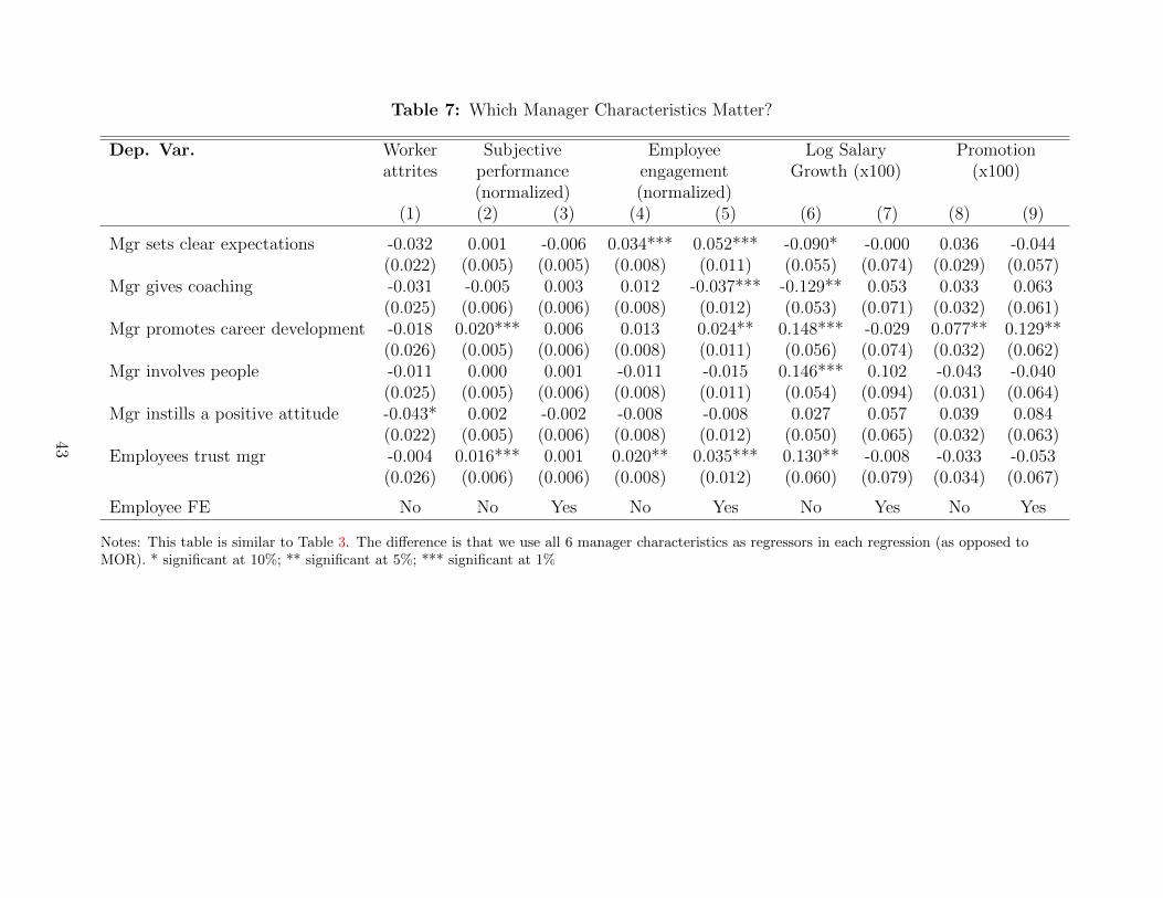
Table 7: Which Manager Characteristics Matter?

Dep. Var. Worker Subjective Employee Log Salary Promotionattrites performance engagement Growth (x100) (x100)

(normalized) (normalized)(1) (2) (3) (4) (5) (6) (7) (8) (9)

Mgr sets clear expectations -0.032 0.001 -0.006 0.034*** 0.052*** -0.090* -0.000 0.036 -0.044(0.022) (0.005) (0.005) (0.008) (0.011) (0.055) (0.074) (0.029) (0.057)

Mgr gives coaching -0.031 -0.005 0.003 0.012 -0.037*** -0.129** 0.053 0.033 0.063(0.025) (0.006) (0.006) (0.008) (0.012) (0.053) (0.071) (0.032) (0.061)

Mgr promotes career development -0.018 0.020*** 0.006 0.013 0.024** 0.148*** -0.029 0.077** 0.129**(0.026) (0.005) (0.006) (0.008) (0.011) (0.056) (0.074) (0.032) (0.062)

Mgr involves people -0.011 0.000 0.001 -0.011 -0.015 0.146*** 0.102 -0.043 -0.040(0.025) (0.005) (0.006) (0.008) (0.011) (0.054) (0.094) (0.031) (0.064)

Mgr instills a positive attitude -0.043* 0.002 -0.002 -0.008 -0.008 0.027 0.057 0.039 0.084(0.022) (0.005) (0.006) (0.008) (0.012) (0.050) (0.065) (0.032) (0.063)

Employees trust mgr -0.004 0.016*** 0.001 0.020** 0.035*** 0.130** -0.008 -0.033 -0.053(0.026) (0.006) (0.006) (0.008) (0.012) (0.060) (0.079) (0.034) (0.067)

Employee FE No No Yes No Yes No Yes No Yes

Notes: This table is similar to Table 3. The difference is that we use all 6 manager characteristics as regressors in each regression (as opposed toMOR). * significant at 10%; ** significant at 5%; *** significant at 1%

43

Table 8: What are Managers Rewarded For? Employees Survey Scores vs. Subjective Performance Score vs. Value-Added

Dep var: Subjective Promoted Log Change in Comp Change in Key Firedperformance (x100) Salary Log ratio span of individual (x100)(normalized) (x100) Salary control (x100)

(x100)(1) (2) (3) (4) (5) (6) (7) (8)

MOR (normalized) 0.067*** -0.031 -0.12 0.35*** 0.012 0.22*** -0.031 -0.015*(0.0072) (0.035) (0.13) (0.052) (0.19) (0.038) (0.22) (0.0089)

Subj performance (normalized) 2.01*** 0.73*** 1.30*** 0.89*** -0.018 5.75*** -0.076***(0.048) (0.098) (0.067) (0.16) (0.041) (0.25) (0.011)

Manager FE in retention 0.014* 0.028 -0.44** -0.29*** 0.44 0.11* 0.42 -0.046***(normalized) (0.0082) (0.041) (0.23) (0.086) (0.34) (0.056) (0.31) (0.011)

R-squared 0.056 0.036 0.947 0.220 0.270 0.026 0.139 0.011

Notes: Standard errors clustered by manager in parentheses. Each column is an OLS regression. An observation is a manager-month. All regressionsinclude the baseline controls as in the OLS regressions in Table 3. “Manager fixed effect in turnover” refers to a manager’s value-added towardemployees in turnover—thus, a lower value-added corresponds to a negative manager fixed effect (i.e., a fixed effect depressing turnover). Thedependent variable “comp ratio” refers to an employees compensation relative to those of employees in comparable jobs in the industry. “Keyindividual” is a dummy variable for whether a manager is designated as key to the firm. “Change in log salary” and “Change in span of control” aredefined as changes relative to 12 months ahead. * significant at 10%; ** significant at 5%; *** significant at 1%

44

“How Do Managers Matter? Evidence from Performance

Metrics and Employee Surveys in a Firm”: Online Ap-

pendix

Mitchell Hoffman and Steven Tadelis

The Online Appendix is organized as follows. Appendix A discuss of additional results.Appendix B gives more details on the data. Appendix C presents additional tables and figures.

A Additional Results

MOR and patenting. As mention in Section 4.1, we assume that the “month of innovation”is equal to the month in which the patent application is filed. This assumption is shared byTabakovic and Wollmann (2016), who study how university financial resources (accured fromfootball wins) affect patent applications. In our application, managers are moving around ata high frequency, so it is fairly important to measure when exactly the innovation is occur-ring. However, we focus on patent applications instead of patents because patents often takemultiple years before they are approved. We also assign one patent for each inventor on thepatent.

In Table C6, the dependent variable is patents developed by an employee in the month.Using all employees in column 1, there is no significant relationship between MOR and patent-ing. Part of this likely reflects that patenting is a high-skill activity that is often concentratedamong high-skill employees, particularly those in scientific areas. Thus, in column 2, we re-strict the sample to employees in engineering. In column 3, we further restrict to US-basedengineers to attempt to further isolate high-skill individuals who are likely to be in a potentialposition to develop patents. Here, we observe a marginally statistically significant relationshipbetween MOR and patenting. While statistical significance is limited, the economic signif-icance of the coefficient is quite sizable. Specifically, a 1σ increase in MOR is associatedwith roughly a 20% increase in patent filing each month (based on comparing the size of thecoefficient to the mean of the dependent variable).

Principal component analysis. We created the principal components using thepooled dataset created by firm analysts at the employee-month level.1 In this data, a givenmanager appears multiple times, reflecting the multiple years of the survey, as well as man-agers who manage multiple employees. To check robustness, we repeated creating the principalcomponents using individual waves of the manager survey scores (where an observation is amanager) and this led to very similar components created.

1We used the “pca” command in Stata.

1

B Data Appendix

Data assembly. The data were assembled for us by an analyst at the data provider. Avariety of files were combined together during this process. The analyst also subjected thedata to cleaning.

Manager overall rating. We focus on results in the text using normalized manageroverall rating. We normalize over all functions including all years in the data. As a robustnesscheck, we will also consider alternative methods of doing the normalization.

Salary. Workers at the firm are paid in different currencies. We convert salaries to USdollars using the exchange rate as of March 1, 2014, which falls in the middle of our dataperiod. We avoid using a time-varying exchange rate because this would induce variation ina worker’s salary over time that may be artificial from the standpoint of a worker located ina foreign country.2

Patents. We collected information on patent applications using Google Patents. InJanuary 2016, an RA obtained information on the patent applications where the firm is listedas the assignee. We then merged the inventor names to the names listed in the employeedatabase.

Key individual. Persons at the firm who are recognized as an integral part of thecompany are designated “key individuals.” The firm uses a slightly different term to refer tosuch persons, but we have modified it for the paper to preserve firm confidentiality.

B.1 Qualitative Findings

Qualitative data from the surveys generally support the importance of managers. For exam-ple, one employee said that most people who are leaving the firm are doing so because of badmanagers (as opposed to business issues). This employee that bad managers causing individ-uals to leave was a central issue that needed to be addressed. Another employee focused onhis/her own manager and described them in a very positive light. The employee reported thatthe manager was providing him/her with the tools to be successful within the company andto support him/her in their development.

B.2 Y3 Survey Questions

The survey questions were slightly different for the Y3. They are listed below.

1. My immediate manager provides ongoing coaching and guidance on how I can improvemy performance.

2. My immediate manager actively supports my efforts regarding professional / careerdevelopment.

3. My immediate manager extends influence and leadership across organizational bound-aries.

2Another approach would be to restrict our analysis of salary to employees who get paid in US dollars, asin Baker et al. (1994a). However, this would require throwing out a lot of our sample.

2

4. My immediate manager creates the conditions that support stronger engagement atwork.

5. I would recommend my manager to others.

3

C Additional Figures and Tables

4

Table C1: Manager Characteristics, Correlation Table

Variables: Clear Coaching Career dev Involves Positive Someoneexpectations people attitude I trust

Manager gives clear expectations 1.00Manager provides coaching 0.67 1.00Manager supports career development 0.59 0.71 1.00Manager involves people 0.59 0.57 0.59 1.00Manager instills positive attitude 0.59 0.58 0.60 0.68 1.00Manager is someone I trust 0.63 0.60 0.64 0.69 0.72 1.00

Notes: Correlation coefficients are reported. The analysis sample (including all data, non-imputed and imputed) has been collapsed to themanager-survey period level.

5

Table C2: Robustness Analysing on Persistence of Managerial Characteristics: Using all the Manager Characteristics asRegressors at the Same Time

(1) (2) (3) (4) (5) (6) (7)Dep. Variables: Overall Clear Coaching Career dev Involves Positive Someone

MOR expectations people attitude I trust

Manager sets clear expectations 0.07* 0.17*** 0.06 0.04 0.07* 0.03 0.06(0.04) (0.04) (0.05) (0.04) (0.04) (0.05) (0.04)

Manager gives coaching 0.04 0.04 0.15*** 0.07* -0.00 -0.01 -0.01(0.03) (0.03) (0.04) (0.04) (0.03) (0.04) (0.04)

Manager promotes career development 0.07** 0.05 0.09** 0.13*** 0.04 0.07* 0.05(0.03) (0.03) (0.04) (0.04) (0.03) (0.04) (0.04)

Manager involves people 0.04 0.02 -0.00 0.03 0.18*** 0.02 0.01(0.04) (0.04) (0.05) (0.05) (0.04) (0.05) (0.05)

Manager instills a positive attitude 0.09** 0.02 0.04 0.09** 0.03 0.23*** 0.11***(0.03) (0.04) (0.05) (0.05) (0.04) (0.04) (0.04)

Employees trust the manager 0.05 0.03 0.01 0.00 0.03 0.06 0.15***(0.04) (0.04) (0.05) (0.05) (0.04) (0.05) (0.05)

R-squared 0.32 0.31 0.33 0.29 0.26 0.28 0.26

Notes: This table is a robustness check to Table 2. Instead of regressing a particular Y2 characteristic on the same characteristic in Y1 and variouscontrols, we regress each Y2 characteristics on all the Y1 characteristics at once (plus controls). * significant at 10%; ** significant at 5%; ***significant at 1%

6

Table C3: Robustness Analysing on Persistence of Managerial Characteristics: Using theY3 Survey

(1) (2)Variables: Overall Overall

MOR MOR

Sample: Y3 Y1, Y2, Y3

Lagged MOR 0.36*** 0.32***(0.078) (0.029)

R-squared 0.24 0.25

Notes: This table is a robustness check to Table 2. The difference is that we use all three surveys (inY1, Y2, Y3) as opposed to just the Y1 and Y2 surveys. Column 1 analyzes MOR in Y3 as a function of MOR inY2. Column 2 analyzes MOR in Y2 and Y3 as a function of the MOR in the previous period. * significant at10%; ** significant at 5%; *** significant at 1%

Table C4: Relationship between Manager Scores and Employee Attrition: DifferentMeasures of Attrition in Hazard Models

Dep var: Quit Fire Quit, regretted Quit, non-regretted(1) (2) (3) (4)

Normalized MOR -0.097*** -0.086*** -0.096*** -0.162***(0.019) (0.024) (0.021) (0.038)

Notes: Standard errors clustered by employee in parentheses. Each column is a Cox proportional hazardregression (with coefficients shown). The failure event is some version of whether an employee attrites in agiven month, looking separately at quits, fires, regretted quits, and non-regretted quits. An observation is anemployee-month. All regressions include controls for business unit, for work type (engineer, customer service,or other), for being a domestic worker, and dummies for month-year of hire. * significant at 10%; **significant at 5%; *** significant at 1%

7

Table C5: Relationship between Manager Scores and Employee Attrition, OLS

Sample: All Engineer CS US Non-US(1) (2) (3) (4) (5)

Normalized MOR (X 100) -0.125*** -0.140*** -0.056*** -0.135*** -0.107***(0.011) (0.023) (0.020) (0.014) (0.016)

Notes: Standard errors clustered by employee in parentheses. Each column is a regression. The dependentvariable is whether an employee attrites in a given month. An observation is an employee-month. Allregressions include controls for business unit, for work type (engineer, customer service, or other), for being adomestic worker, a third-order polynomial in tenure, and dummies for month-year of hire. * significant at10%; ** significant at 5%; *** significant at 1%

Table C6: Relationship between Manager Scores and Employee Patents, OLS

Sample: All Engineer US Engineer US EngineerHigher salary grade

(1) (2) (3) (4)

Normalized MOR 0.0011 0.0102 0.0167* 0.0202(0.0018) (0.0063) (0.00897) (0.0127)

Mean dep var 0.0166 0.0513 0.0680 0.0875

Notes: Standard errors clustered by manager in parentheses. Each column is a regression. The dependentvariable is the number of patent applications filed by an employee in a given month. An observation is anemployee-month. Controls are the same as in column 2 of Table 3. * significant at 10%; ** significant at 5%;*** significant at 1%

8

Table C7: MOR and Employee Outcomes: Results using Not the Current Period

Worker Subjective Employee Log Salary Promotionattrites performance engagement Growth (x100) (x100)

(normalized) (normalized)(1) (2) (3) (4) (5) (6) (7) (8) (9)

Panel A: AllMOR (normalized) -0.116*** 0.031*** 0.006 0.031*** 0.006* 0.119** 0.097** -0.018 0.106

(0.015) (0.005) (0.005) (0.007) (0.003) (0.059) (0.050) (0.031) (0.074)

Panel B: EngineersMOR (normalized) -0.090*** 0.016* 0.000 0.003 0.003 -0.024 0.053 -0.023 0.113

(0.028) (0.009) (0.009) (0.012) (0.009) (0.108) (0.122) (0.032) (0.080)

Employee FE No No Yes No Yes No Yes No Yes

Notes: Standard errors clustered by manager in parentheses. All regressions include controls for business unit, for work type (engineer, customerservice, marketing, finance, or other), dummies for year of hire (observations before 2001 lumped in one year), salary grade dummies, current yeardummies, and location dummies. Column 1 is a Cox proportional hazard regression (with coefficients shown). The failure event is whether anemployee attrites in a given month. Tenure is controlled for non-parametrically. Locations with less than 2,000 employee-months are lumped into aseparate location category. Columns 2-9 show OLS regressions, and tenure is controlled for using a 5th order polynomial. Locations with less than 10employee-months are lumped into a separate location category. “Subjective performance” is an employee’s subjective performance on a 1-5 scale.“Employee Engagement” is normalized employee engagement. In columns 8-9, the outcome is whether an employee receives a promotion, withcoefficients multiplied by 100 for readability. * significant at 10%; ** significant at 5%; *** significant at 1%

9

Table C8: Manager Value-Added Estimates for Employee Attrition

Method: OLS Supervisor SupervisorFixed Effects Random Effects

R-squared 0.0062 0.0219

Mean term rate 0.0178SD boss effects 0.0198 0.0102F-stat on boss effects 1.631

Notes: Columns 1-2 include a 3rd order polynomial in tenure, year of hire dummies, and current yeardummies. Column 3 includes controls for work type (engineer, customer service, or other), year of hire, andcurrent year. The fixed effect standard deviations are weighted by the number of observations per fixedeffect. * significant at 10%; ** significant at 5%; *** significant at 1%

Table C9: Manager Value-Added Estimates for Employee Salaries

Method: OLS Worker Supervisor SupervisorFE FE & Worker FE

(1) (2) (3) (4)

R-squared 0.0625 0.99 0.8965 0.9911

SD of boss effects 0.24 0.075F-stat on boss effects 11.69***

SD of worker effects 0.186 0.185F-stat on worker effects 195.97***

Notes: All regressions include a 3rd order polynomial in tenure, year of hire dummies, and current yeardummies. After estimation, the fixed effects are residualized using a dummy for being an engineer, a dummyfor being a CS worker, location dummies, and salary grade dummies. The fixed effect standard deviationsare weighted by the number of observations per fixed effect. * significant at 10%; ** significant at 5%; ***significant at 1%

10

Table C10: Do Managers Matter for Quitting?

Method: OLS Supervisor SupervisorFixed Effects Random Effects

R-squared 0.0034 0.0162

Mean quit rate 0.01SD boss effects 0.0124 0.0056F-stat on boss effects 1.317

Notes: This table is similar to Table C8 except that it analyzes quitting as the outcome instead of overallattrition. * significant at 10%; ** significant at 5%; *** significant at 1%

Table C11: Do Managers Matter for Firing?

Method: OLS Supervisor SupervisorFixed Effects Random Effects

R-squared 0.0075 0.0231

Mean fire rate 0.0045SD boss effects 0.0093 0.0061F-stat on boss effects 1.622

Notes: This table is similar to Table C8 except that it analyzes firing as the outcome instead of overallattrition. * significant at 10%; ** significant at 5%; *** significant at 1%

11

Table C12: Principal Component Analysis

Variables: Component Component Component Component1 2 3 4

Eigenvalue 4.34 0.54 0.36 0.30Proportion variance explained 0.72 0.09 0.06 0.05

Manager gives clear expectations 0.40 0.38 0.74 0.10Manager provides coaching 0.41 0.55 -0.14 -0.12Manager supports career development 0.41 0.27 -0.64 0.01Manager involves people 0.41 -0.38 -0.04 0.80Manager instills positive attitude 0.41 -0.44 0.09 -0.51Manager is someone I trust 0.42 -0.37 0.02 -0.27

Notes: This table presents the results of the principal components analysis.

12

Table C13: Robustness on What are Managers Rewarded For? Don’t Include Manager Subjective Performance or ManagerFE in Turnover

Dep var: Subjective Promoted Log Change in Comp Change in Key Firedperformance (x100) Salary Log ratio span of individual (x100)(normalized) (x100) Salary control (x100)

(x100)(1) (2) (3) (4) (5) (6) (7) (8)

MOR (normalized) 0.067*** 0.10*** -0.077 0.39*** 0.080 0.24*** 0.34 -0.025***(0.0072) (0.033) (0.12) (0.052) (0.19) (0.038) (0.21) (0.0088)

R-squared 0.055 0.017 0.947 0.191 0.268 0.025 0.112 0.010

Notes: This table is a robustness check for Table 8. The difference is that we don’t include the managers own subjective performance score or themanager’s value-added coefficient as regressors. * significant at 10%; ** significant at 5%; *** significant at 1%

13

Appendix References

Baker, George P., Michael Gibbs, and Bengt Holmstrom, “The Wage Policy of aFirm,” Quarterly Journal of Economics, 1994, 109 (4), pp. 921–955.

Tabakovic, Haris and Thomas Wollmann, “The Impact of Money on Science: Evidencefrom Unexpected NCAA Football Outcomes,” 2016. Mimeo, University of Chicago.

14