horizontal mapping accuracy in hydrographic auv surveys

Horizontal Mapping Accuracy in HydrographicAUV Surveys

Øyvind Hegrenæs∗, Torstein Olsmo Sæbø†, Per Espen Hagen∗, Bjørn Jalving∗

∗Kongsberg Maritime Subsea, AUV Department, NO-3191 Horten, Norway†Norwegian Defence Research Establishment, NO-2027 Kjeller, Norway

Abstract— Underwater vehicles are used in a wide range oftasks in various sectors. Cost-effective and accurate seabedsurveying and mapping using autonomous underwater vehicles(AUVs) have been carried out for years in the offshore oil andgas sector. Much of the experience gained is now being benefitedupon in new and challenging applications. One of the emergingAUV applications is hydrographic surveying (e.g. for creatingnautical charts), particularly in waters shallower than 100 m.Key factors for mission-success include obtainable accuracy andresolution of the final digital terrain model (DTM), as well asthe feature detection capability of the integrated system.

This paper gives an in-depth discussion and analysis of thehorizontal mapping accuracy achievable by integrated, state-of-the-art hydrographic AUV systems. The HUGIN 1000 AUV fittedwith interferometric synthetic aperture sonar (SAS) is used asa case study, and the system accuracy as assessed in detail –starting from surface navigation, going all the way down to theacoustic seabed footprint. A discussion is given at the end on thefeasibility of AUVs in terms of the minimum standards proposedby the International Hydrographic Organization (IHO).

I. INTRODUCTION

Autonomous underwater vehicles (AUVs) have proved im-pressive performance in commercial seabed mapping oper-ations, both with respect to mapping efficiency and dataquality. While traditional hydrographic surveys for creatinge.g. nautical charts have been carried out using surface basedsystems, an increasing interest is shown toward the use ofAUVs for the same purpose. Part of the reasons are probablythe versatility and multi-disciplinary capability of the AUVs,the stability of the platform and the resulting high-quality high-resolution data, the crew size needed for operations, and notthe least, the ability to carry out missions fully autonomously.

Knowing the accuracy or reliability of the final chart ofdigital terrain model (DTM) is imperative for the end-useror institution. As discussed in this paper, accuracy denotesthe degree of conformity (offset) of a measured or estimatedquantity to its true value. Similarly, precision is the degreeto which repeated samples or measurements under unchangedconditions show the same results (variability). For some ap-plications such as making nautical charts it is crucial thatthe accuracy is high. This is particularly the case in shallowwater. Precision is on the other hand indicative of the ability tobuild fine resolution images, and may therefore be necessaryfor other applications, e.g. archeology or military operationsusing synthetic aperture sonar (SAS). The need for accuracy

may vary in these cases. Due to their versatility, AUVs canfacilitate a wide range of technical needs and applications.

For a DTM the quantities of interest are co-registered depthand position data. A key observation is that the survey end-product has no better accuracy than the least accurate com-ponent in the measurement chain, from surface navigation allthe way down to the acoustic seabed footprint. The accuracyof each component or of the final DTM (total accuracy) maybe stated by an uncertainty and some associate confidencelevel. The purpose of this paper is to discuss and analyze theachievable horizontal mapping accuracy in integrated, state-of-the-art hydrographic AUV systems. While the KongsbergMaritime HUGIN 1000 AUV fitted with HISAS SAS is usedas a case study, most of the results and methodologies applyto other AUVs and traditional hydrographic payloads such asmulti-beam echo sounder (MBE) and side-scan sonar (SSS).

This paper is organized as follows. Section II gives abrief introduction to AUVs, including payload sensors andnavigation. Some details on the HUGIN 1000 AUV and itssensors are given, including examples of data collected withthe HISAS SAS. The paper continues in Section III witha breakdown and analyses of different error sources whichcontribute to the horizontal position uncertainty of the DTMsoundings. Error budgets are presented in Section IV. Adiscussion is also given on the feasibility of AUVs in termsof the standards proposed by the International HydrographicOrganization (IHO). Conclusions are given in Section V.

II. AUVS FOR HYDROGRAPHIC SURVEYING

A. Platforms and Payload Systems

AUVs are available as COTS (commercial, off-the-shelf)systems in a range of sizes and depth ratings. In general,endurance and capability scales with vehicle size. Smallervehicles, such as the REMUS 100, can be equipped withsmall-footprint bathymetric sensors such as a GeoAcousticsGeoSwath. HUGIN 1000, the system described in this article,is a medium-size AUV capable of carrying and operating mul-tiple high-end sensors simultaneously. The vehicle is shown inFig. 1. The vehicle has a dry weight of 600-900 kg depend-ing on configuration, a length of approximately 5 m, and adiameter of 75 cm. A typical military configuration includesthe HISAS 1030 interferometric SAS, an EM 3002 MBE,

In Proceedings of the IEEE AUV Conference, Monterey, CA, USA, 2010.

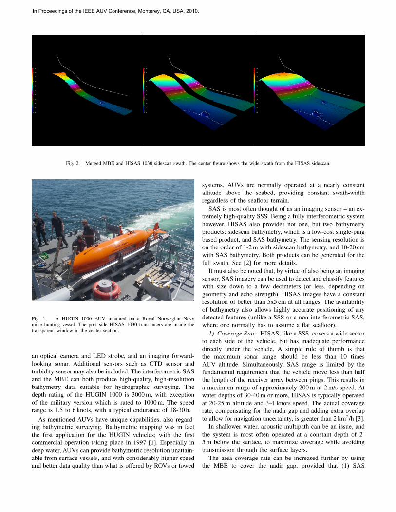
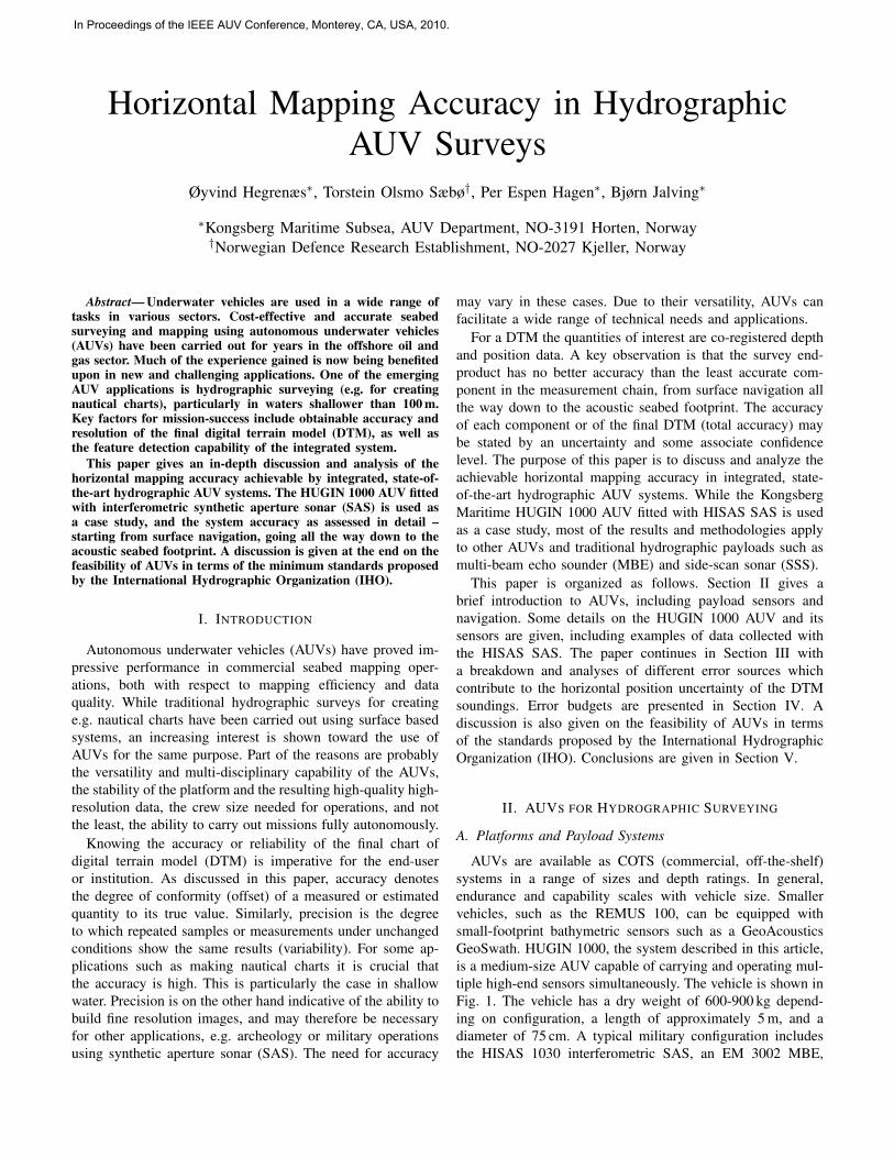
Fig. 2. Merged MBE and HISAS 1030 sidescan swath. The center figure shows the wide swath from the HISAS sidescan.

Fig. 1. A HUGIN 1000 AUV mounted on a Royal Norwegian Navymine hunting vessel. The port side HISAS 1030 transducers are inside thetransparent window in the center section.

an optical camera and LED strobe, and an imaging forward-looking sonar. Additional sensors such as CTD sensor andturbidity sensor may also be included. The interferometric SASand the MBE can both produce high-quality, high-resolutionbathymetry data suitable for hydrographic surveying. Thedepth rating of the HUGIN 1000 is 3000 m, with exceptionof the military version which is rated to 1000 m. The speedrange is 1.5 to 6 knots, with a typical endurance of 18-30 h.

As mentioned AUVs have unique capabilities, also regard-ing bathymetric surveying. Bathymetric mapping was in factthe first application for the HUGIN vehicles; with the firstcommercial operation taking place in 1997 [1]. Especially indeep water, AUVs can provide bathymetric resolution unattain-able from surface vessels, and with considerably higher speedand better data quality than what is offered by ROVs or towed

systems. AUVs are normally operated at a nearly constantaltitude above the seabed, providing constant swath-widthregardless of the seafloor terrain.

SAS is most often thought of as an imaging sensor – an ex-tremely high-quality SSS. Being a fully interferometric systemhowever, HISAS also provides not one, but two bathymetryproducts: sidescan bathymetry, which is a low-cost single-pingbased product, and SAS bathymetry. The sensing resolution ison the order of 1-2 m with sidescan bathymetry, and 10-20 cmwith SAS bathymetry. Both products can be generated for thefull swath. See [2] for more details.

It must also be noted that, by virtue of also being an imagingsensor, SAS imagery can be used to detect and classify featureswith size down to a few decimeters (or less, depending ongeometry and echo strength). HISAS images have a constantresolution of better than 5x5 cm at all ranges. The availabilityof bathymetry also allows highly accurate positioning of anydetected features (unlike a SSS or a non-interferometric SAS,where one normally has to assume a flat seafloor).

1) Coverage Rate: HISAS, like a SSS, covers a wide sectorto each side of the vehicle, but has inadequate performancedirectly under the vehicle. A simple rule of thumb is thatthe maximum sonar range should be less than 10 timesAUV altitude. Simultaneously, SAS range is limited by thefundamental requirement that the vehicle move less than halfthe length of the receiver array between pings. This results ina maximum range of approximately 200 m at 2 m/s speed. Atwater depths of 30-40 m or more, HISAS is typically operatedat 20-25 m altitude and 3-4 knots speed. The actual coveragerate, compensating for the nadir gap and adding extra overlapto allow for navigation uncertainty, is greater than 2 km2/h [3].

In shallower water, acoustic multipath can be an issue, andthe system is most often operated at a constant depth of 2-5 m below the surface, to maximize coverage while avoidingtransmission through the surface layers.

The area coverage rate can be increased further by usingthe MBE to cover the nadir gap, provided that (1) SAS


imaging is not required for the entire area, and (2) thatthe MBE bathymetry has sufficient resolution, accuracy andsample density. A good quality MBE like the EM 3002 hasa resolution matching HISAS sidescan bathymetry, but notSAS bathymetry. An illustration showing the combined use ofHISAS sidescan and MBE is shown in Fig. 2

One of the challenges of operating multiple sensors simul-taneously is that requirements on operational parameters suchas altitude and speed differ between sensors. Fortunately, forbathymetric mapping, there is a considerable range of settingswhere the SAS and the MBE both work very well. The MBEmore than covers the nadir gap of the HISAS. The overlappingregions can be used for quality control, by comparing the datafrom the two sensors.

B. Navigation

The limitations of underwater sensors and the demand forautonomy makes underwater navigation a unique and difficultchallenge. Most AUV navigation systems are today based onan inertial navigation system (INS), which takes measuredangular rates and specific forces from an inertial measurementunit (IMU) as inputs. The INS then calculates the position,orientation and velocity of the vehicle relative to the inertialspace. Due to inherent errors in the IMU however, a pureINS solution will drift of rapidly with time. A navigationgrade INS such as the one installed in HUGIN 1000 driftson the order of 0.8 nmi/h if left unaided. The aiding may bedone using a wide range of sensors, including a depth sensor,acoustic positioning, GPS while at the surface, and someform of velocity aiding. Once a suitable aiding frameworkhas been established, a Kalman filter (KF) is typically appliedfor carrying out the fusion of the disparate sensor data and theINS data. See [4], [5], [6] for a further discussion.

For hydrographic applications the use of ultra-short baseline(USBL) acoustic positioning is the preferred method. The useof Kongsberg Maritime HiPAP USBL is discussed later inthis paper in regards to achievable mapping accuracy. Theuse of surface GPS fixes is also discussed. This may bethe only feasible solution in very shallow water or whenfully autonomous missions are desirable, or even required.The importance of proper velocity aiding in cases wherepositioning is sparse should be emphasized.

1) Accuracy Enhancement in Post-Processing: When dis-cussing underwater navigation, it is important to distinguishbetween performance in real-time and after post-processing.The real-time performance obviously determines where theAUV actually collects its data. Depending on the application, itmay be desirable to enhance the navigation precision further inpost-processing. This is standard procedure for all the HUGINAUVs, where the post-processing is carried out using NavLab[7]. NavLab is a simulation and navigation post-processingtool which has been used extensively with all the HUGINAUVs since the late 1990’s. In addition to re-navigating thereal-time (based on experimental or simulated data) navigationsystem, NavLab also contains offline smoothing functionality,based on a Rauch-Tung-Striebel (RTS) implementation. The

RTS smoother utilizes both past and future sensor measure-ments and KF covariances, hence significantly improving theintegrity and accuracy of the final navigation solution [8].

III. HORIZONTAL MAPPING ACCURACY

The total horizontal uncertainty (THU) of a DTM is to beunderstood as the uncertainty of the combined AUV positionsand sounding footprint positions. As mentioned in Section II,there are in principle two ways of carrying out AUV missions;fully autonomous or supervised, and by utilizing AUV surfaceGPS or some form of acoustic positioning in order to boundthe navigation system position error drift. Uncertainties relatedto these systems and other components further down in themeasurement chain are discussed subsequently in relation totheir contribution to the THU. Many of the contributions areincluded in the DTM error budget in Section IV. Part of thematerial is motivated by the work carried out in [9]. Someother relevant work can also be found in [10], [11], [12].

A. AUV Related Uncertainties

The following gives a discussion on uncertainties related tothe horizontal positioning of the AUV. The HUGIN AUV andthe HiPAP USBL system discussed in Section II are used ascase studies. With few exceptions the material applies to otherintegrated hydrographic AUV systems as well.

1) GPS accuracy: Several GPS services applicable forAUV survey systems are available:• GPS standard positioning service (SPS)• GPS precise positioning service (PPS)• Differential GPS (DGPS)• Real-time kinematic GPS (RTKGPS)• GPS precise point positioning (PPP)

SPS and PPS are both available worldwide, but PPS is only forauthorized users and primarily intended for military purposes.Stand-alone single-frequency (L1) SPS solutions exist whichhave a horizontal accuracy on the order of 2 m (1σ). Dualfrequency (L1/L2) yields slightly better performance. Furtheraccuracy improvement is achieved by incorporating correctiondata broadcasted from stationary reference stations. This isthe case for both DGPS and RTKGPS. The systems differ inthe use of code-phase and carrier-phase techniques, where thelatter yields the best performance. DGPS typically provides ahorizontal accuracy on the order of 0.5 m (1σ) while RTKGPShas an accuracy ranging from about 0.2 m (1σ) down to afew centimeters or less. A post-processing alterative to DGPSand RTKGPS which does no rely on a reference stationinfrastructure is GPS PPP. By fusing raw carrier-phase datafrom a single GPS SPS receiver (typically dual-frequency)with precise ephemerides and satellite clock corrections (freelyavailable from the Internet), PPP yields an accuracy close toRTKGPS. See [13], [14] for a further discussion on GPS PPP.

All the above mentioned GPS techniques and accuracynumbers are feasible for a surface ship, and hence for beingused in the fusion with USBL acoustic position measurements.For the GPS mounted on an AUV the situation is more


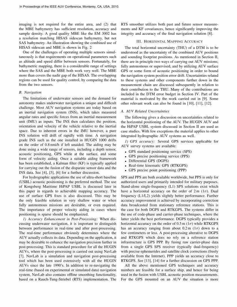
Fig. 3. Kongsberg Maritime HiPAP measurement principle

challenging due to the requirement of a pressure tolerantantenna. While a pressure tolerant molding satisfies part ofthis requirement it also leads to challenges related to dampingand frequency shifts. Consequently a COTS antenna may notlonger work as expected, and one might end up having to do acomplete antenna re-design, where a single-frequency antennais the easiest. This work has been done for the HUGIN AUVswhere the GPS antenna (L1), WLAN, and Iridium are fittedin one molding, depth rated to 6000 m. The horizontal GPSaccuracy for this unit is about 1.8 m (1σ).

It should be mentioned that the GPS receiver onboard theHUGIN AUVs may process DGPS and RTKGPS corrections.One possibility is to forward this information from e.g. thesurface vessel to the AUV via a radio link or Iridium. Anotheralternative is to base the system on SBAS (satellite-based aug-mentation system). While neither are currently implemented itis believed that horizontal GPS accuracy somewhere between0.6 and 0.2 m (1σ) is achievable for demanding AUV opera-tions. Finally note that GPS PPP is not currently feasible forcarrying out typical GPS surface fixes with an AUV since thetechnique requires fairly long sequences of data to converge.

2) Acoustic positioning: While acoustic time of flight nav-igation has been around for decades, it is still today the mostreliable position aiding tool while (deeply) submerged. Severalapproaches are available [15], [16], where LBL and UBSLare the most common within AUV navigation. An increasingnumber of single-transponder and synchronous-clocks systemshave also been proposed as alternatives to LBL and USBL. Thereader is referred to [17], [18], [19], and references therein fora further treatment. Only USBL is discussed in this paper.

As for USBL, a typical approach is to measure the rangeand bearing (azimuth and elevation) of a transponder on theunderwater vehicle relative to a transducer mounted on asurface vessel. A global position measurement, which maybe transmitted to the submersible using an acoustic link,

can be obtained by combining surface ship GPS and USBLmeasurements. The USBL principle is illustrated in Fig. 3 forthe HiPAP USBL system. The following sources affect thecombined GPS-USBL position estimate:

• GPS accuracy (as discussed in Section III-A.1)• USBL measurement accuracy• System installation accuracy• Surface ship attitude accuracy• Sound velocity profile (SVP) accuracy

A general expression for the north-east-down (NED) posi-tion of the AUV relative to the ship is given as

pn = Rnb (φ, θ, ψ)Rb

t(φ′, θ′, ψ′)pt(Γ, α, γ), (1)

where pt ∈ R3 is the position of the AUV measured relative tothe USBL transducer, represented in the transducer referenceframe {t}. The position vector pt may be represented usingspherical coordinates where Γ is the measured slant range, andα and γ are measured azimuth and elevation, respectively.Furthermore Rb

t ∈ SO(3) is a coordinate transformationmatrix from {t} to the ship reference frame {b} (or alter-natively, the rotation matrix from {b} to {t}). The last matrixRn

b ∈ SO(3) is the coordinate transformation matrix from{b} to the NED frame {n}. The transformation matrices maybe represented in many ways, but it is common to apply thezyx-convention using Euler angles [20]. The measured surfaceship roll, pitch and heading are given by φ, θ, ψ, respectively,while φ′, θ′, ψ′ describe the transducer alignment offset inroll, pitch and heading. Note that the latter angles are notgeographical angles, but generic roll, pitch and heading Eulerangles. Typically the transducer is mounted such that the latterangles are small. Note that the expression in (1) could haveincluded an additional additive term Rn

b (φ, θ, ψ)pbo, where pb

o

is the offset (lever-arm) between {b} and {t}. With the purposeof doing error analysis the term is however disregarded sincelinear offsets between {b} and {t} can be measured withinmillimeters (the same is also the case for the ship GPSantenna). The uncertainty introduced through Rn

b when doinglever-arm compensation is also negligible compared to theother error sources when ‖pb

o‖ � ‖pt‖. For brevity it isassumed that {b}, {t} and {n} share the same origin.

A common approach in error analysis is to look at eachisolated error source and to propagate the uncertainties [21].This approach is used in this paper when analytical closed-form expressions are available. As for (1) a natural start isto look at the uncertainty in the horizontal position due touncertainty in pt, i.e. USBL measurement uncertainty. If forthe moment it is assumed that Rb

t and Rnb are exact and equal

to the identity matrix (all the angles are zero) we get that

pn = pt(Γ, α, γ), (2)

which means that an error in pt directly translates to a(geographical) horizontal and vertical position error. With theassumption of small errors (first order approximation), the


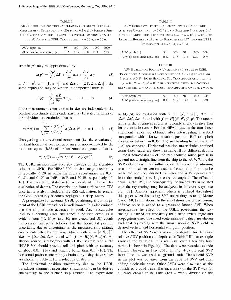
TABLE IAUV HORIZONTAL POSITION UNCERTAINTY (1σ) DUE TO HIPAP 500

MEASUREMENT UNCERTAINTY AT 20 DB AND 0.2 M (1σ) SURFACE SHIP

GPS UNCERTAINTY. THE RELATIVE HORIZONTAL POSITION BETWEEN

THE AUV AND THE USBL TRANSDUCER IS X = 50 M, Y = 50 M.

AUV depth [m] 50 100 500 1000 3000AUV position uncertainty [m] 0.32 0.35 1.08 2.11 6.29

error in pn may be approximated by

∆pn =∂pt

∂Γ∆Γ +

∂pt

∂α∆α+

∂pt

∂γ∆γ. (3)

If f := pt, x := [Γ, α, γ]> and ∆x := [∆Γ,∆α,∆γ]>, thesame expression may be written in component form as

∆pni =3∑

j=1

∂fi

∂xj∆xj , i = 1, . . . , 3. (4)

If the measurement error entries in ∆x are independent, theposition uncertainty along each axis may be stated in terms ofthe individual uncertainties, that is,

σ(∆pni ) =

√√√√ 3∑j=1

(∂fi

∂xj

)2

σ(∆xj)2, i = 1, . . . , 3. (5)

Disregarding the directional component (i.e. the covariance),the final horizontal position error may be approximated by theroot-sum-square (RSS) of the horizontal components, that is,

σ(∆pnh) =√σ(∆pn1 )2 + σ(∆pn2 )2. (6)

The USBL measurement accuracy depends on the signal-to-noise ratio (SNR). For HiPAP 500 the slant range uncertaintyis typically < 20 cm while the angle uncertainties are 0.3◦,0.18◦, and 0.12◦ at 0 dB, 10 dB and 20 dB, respectively (all1σ). The uncertainty stated in (6) is calculated in Table I fora selection of depths. The contribution from surface ship GPSuncertainty is also included in the RSS calculation. In generalthe GPS uncertainty becomes negligible in deep waters.

A prerequisite for accurate USBL positioning is that align-ment of the USBL transducer is well known. It is also eminentthat the ship attitude accuracy is good. Any inaccuracieslead to a pointing error and hence a position error, as isevident from (1). If pt and Rb

t are exact, and Rbt equals

the identity matrix, it follows that the horizontal positionuncertainty due to uncertainty in the measured ship attitudecan be calculated by applying (4)-(6), with x := [φ, θ, ψ]>,∆x := [∆φ,∆θ,∆ψ]>, and with f := Rn

b (φ, θ, ψ)pt. Anattitude sensor used together with a UBSL system such as theHiPAP 500 should provide roll and pitch with an accuracyof about 0.01◦ (1σ) and heading better than 0.1◦ (1σ). Thehorizontal position uncertainty obtained by using these valuesare shown in Table II for a selection of depths.

The horizontal position uncertainty due to the USBLtransducer alignment uncertainty (installation) can be derivedanalogously to the surface ship attitude. The expressions

TABLE IIAUV HORIZONTAL POSITION UNCERTAINTY (1σ) DUE TO SHIP

ATTITUDE UNCERTAINTY OF 0.01◦ (1σ) IN ROLL AND PITCH, AND 0.1◦

(1σ) IN HEADING. THE SHIP ATTITUDE IS φ = 0◦, θ = 0◦, ψ = 0◦ . THE

RELATIVE HORIZONTAL POSITION BETWEEN THE AUV AND THE USBLTRANSDUCER IS X = 50 M, Y = 50 M.


TABLE IIIAUV HORIZONTAL POSITION UNCERTAINTY (1σ) DUE TO USBL

TRANSDUCER ALIGNMENT UNCERTAINTY OF 0.05◦ (1σ) IN ROLL AND

PITCH, AND 0.1◦ (1σ) IN HEADING. THE TRANSDUCER ALIGNMENT IS

φ′ = 0◦ , θ′ = 0◦ , ψ′ = 0◦ . THE RELATIVE HORIZONTAL POSITION

BETWEEN THE AUV AND THE USBL TRANSDUCER IS X = 50 M, Y = 50 M.


in (4)-(6), are evaluated with x := [φ′, θ′, ψ′]>, ∆x :=[∆φ′,∆θ′,∆ψ′]>, and with f := Rb

t(φ′, θ′, ψ′)pt. The uncer-

tainty in the alignment angles is typically slightly higher thanfor the attitude sensor. For the HiPAP systems the transduceralignment values are obtained after interrogating a seabedtransponder with a known absolute position. Roll and pitchaccuracies better than 0.05◦ (1σ) and heading better than 0.1◦

(1σ) are expected. Horizontal position uncertainties obtainedusing these values are shown in Table III for different depths.

For a non-constant SVP the true acoustic sound path is ingeneral not a straight line from the ship to the AUV. While theSVP only has a minor influence on the acoustic positioningnear the transducer vertical (nadir), the sound profile must bemeasured and compensated for when the AUV operates farfrom the vertical (i.e. large elevation angles). The effect oferrors in the SVP, and consequently the uncertainty associatedwith the ray-tracing, may be analyzed in different ways, seee.g. [12]. Another approach, which is utilized throughoutthis paper when discussing SVP uncertainty, is to do MonteCarlo (MC) simulations. In the simulations performed herein,additive noise is added to a presumed known SVP. Wheninvestigating the effect on the USBL positioning the ray-tracing is carried out repeatedly for a fixed arrival angle andpropagation time. The fixed (deterministic) values are chosensuch that ray-tracing with the known nominal SVP yields adesired vertical and horizontal end-point position.

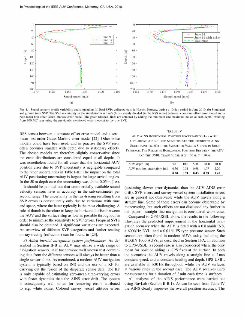
The effect of SVP errors where investigated for the samerelative AUV position and depths as in Table I-III. An exampleshowing the variations in a real SVP over a ten day timeperiod is shown in Fig. 4(a). The data were recorded outsideHorten, Norway, in June 2010. In Fig. 4(b) the real SVPfrom June 14 was used as ground truth. The second SVPin the plot was obtained from the June 14 SVP and afteradding stochastic noise. Other SVPs were also used as theconsidered ground truth. The uncertainty of the SVP was forall cases chosen to be 1 m/s (1σ) – evenly divided (in the


Sound speed [m/s]

Depth

[m]

June 9June 14June 18

1470 1475 1480 1485 1490 1495

0

20

40

60

80

100

120

140

160

180

200

(a)

Sound speed [m/s]

Depth

[m]

June 14June 14 with noiseMax error

1465 1470 1475 1480 1485 1490 1495

0

20

40

60

80

100

120

140

160

180

200

(b)

Fig. 4. Sound velocity profile variability and simulation: (a) Real SVPs collected outside Horten, Norway, during a 10 day period in June 2010. (b) Simulatedand ground truth SVP. The SVP uncertainty in the simulation was 1 m/s (1σ) – evenly divided (in the RSS sense) between a constant offset error model and azero-mean first order Gauss-Markov error model. The green (dashed) lines are obtained by adding the minimum and maximum noises at each depth (resultingfrom 100 MC runs using the previously mentioned error models) to the true SVP.

RSS sense) between a constant offset error model and a zero-mean first order Gauss-Markov error model [22]. Other noisemodels could have been used, and in practise the SVP erroroften becomes smaller with depth due to stationary effects.The chosen models are therefore slightly conservative sincethe error distributions are considered equal at all depths. Itwas nonetheless found for all cases that the horizontal AUVposition error due to SVP uncertainty is negligible comparedto the other uncertainties in Table I-III. The impact on the totalAUV positioning uncertainty is largest for large arrival angles.In the 50 m depth case the uncertainty was about 0.05 m (1σ).

It should be pointed out that commercially available soundvelocity sensors have an accuracy in the sub-centimeter persecond range. The uncertainty in the ray-tracing resulting fromSVP errors is consequently only due to variations with timeand space, where the latter typically is the most challenging. Arule of thumb is therefore to keep the horizontal offset betweenthe AUV and the surface ship as low as possible throughout inorder to minimize the sensitivity to SVP errors. Frequent SVPsshould also be obtained if significant variations are expected.An overview of different SVP categories and further readingon ray-tracing (refraction) can be found in [23].

3) Aided inertial navigation system performance: As de-scribed in Section II-B an AUV may utilize a wide range ofnavigation sensors. It if furthermore well known that combin-ing data from the different sensors will always be better than asingle sensor alone. As mentioned, a modern AUV navigationsystem is typically based on INS and the use of a KF forcarrying out the fusion of the disparate sensor data. The KFis only capable of estimating zero-mean time-varying errorswith faster dynamics than the AINS error drift. The systemis consequently well suited for removing errors attributedto e.g. white noise. Colored survey vessel attitude errors

TABLE IVAUV AINS HORIZONTAL POSITION UNCERTAINTY (1σ) WITH

GPS-HIPAP AIDING. THE NUMBERS ARE THE PREDICTED AINSUNCERTAINTIES, WITH THE SMOOTHED VALUES SHOWN IN BOLD

TYPEFACE. THE RELATIVE HORIZONTAL POSITION BETWEEN THE AUVAND THE USBL TRANSDUCER IS X = 50 M, Y = 50 M.


0.20 0.21 0.43 0.69 1.45

(assuming slower error dynamics than the AUV AINS errordrift), SVP errors and survey vessel system installation errorsare in general not observable while the AUV travels along astraight line. Some of these errors can become observable bymaneuvering, but such effects are not discussed any further inthis paper – straight line navigation is considered worst-case.

Compared to GPS-USBL alone, the results in the followingillustrates the predicted improvement in the horizontal navi-gation accuracy when the AUV is fitted with a 0.8 nmi/h INS,a 600 kHz DVL, and a 0.01 % FS type pressure sensor. Suchsensors are often found in modern AUVs today, including theHUGIN 1000 AUVs, as described in Section II-A. In additionto GPS-USBL, a second case is also considered where the onlymean for position aiding is GPS fixes at the surface. In boththe scenarios the AUV travels along a straight line at 2 m/sconstant speed, and at constant heading and depth. GPS-USBLare available at 1/30 Hz throughout, while the AUV surfacesat various rates in the second case. The AUV receives GPSmeasurements for a duration of 2 min each time is surfaces.

All analyzes of the AINS performance were carried outusing NavLab (Section II-B.1). As can be seen from Table IVthe AINS clearly improves the overall position accuracy. The


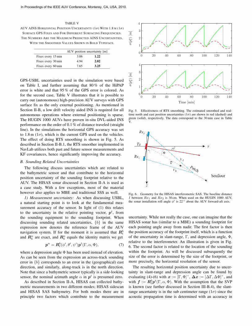
TABLE VAUV AINS HORIZONTAL POSITION UNCERTAINTY (1σ) WITH 1.8 M (1σ)

SURFACE GPS FIXES AND FOR DIFFERENT SURFACING FREQUENCIES.THE NUMBERS ARE THE MAXIMUM PREDICTED AINS UNCERTAINTIES,

WITH THE SMOOTHED VALUES SHOWN IN BOLD TYPEFACE.

AUV position uncertainty [m]

Fixes every 15 min 3.06 1.22Fixes every 30 min 4.94 2.02Fixes every 60 min 7.65 3.25

GPS-USBL uncertainties used in the simulation were basedon Table I, and further assuming that 80 % of the HiPAPerror is white and that 95 % of the GPS error is colored. Asfor the second case, Table V illustrates that it is possible tocarry out (autonomous) high-precision AUV surveys with GPSsurface fix as the only external positioning. As mentioned inSection II-B, a low drift velocity aided INS is required for allautonomous operations where external positioning is sparse.The HUGIN 1000 AUVs have proven in-situ DVL-aided INSperformance on the order of 0.1 % of distance traveled (straightline). In the simulations the horizontal GPS accuracy was setto 1.8 m (1σ), which is the current GPS used on the vehicles.The effect of doing RTS smoothing is shown in Fig. 5. Asdescribed in Section II-B.1, the RTS smoother implemented inNavLab utilizes both past and future sensor measurements andKF covariances, hence significantly improving the accuracy.

B. Sounding Related Uncertainties

The following discuss uncertainties which are related tothe bathymetric sensor and that contribute to the horizontalposition uncertainty of the sounding footprint relative to theAUV. The HISAS sonar discussed in Section II-A is used asa case study. With a few exceptions, most of the materialhowever also applies to MBE and traditional SSS as well.

1) Measurement uncertainty: As when discussing USBL,a natural starting point is to look at the fundamental mea-surement accuracy of the sensor. In light of (1) this relatesto the uncertainty in the relative pointing vector, pt, fromthe sounding equipment to the sounding footprint. Whendiscussing sounding related uncertainties, {b} in the sameexpression now denotes the reference frame of the AUVnavigation system. If for the moment it is assumed that Rb

t

and Rnb are exact, and Rn

b equals the identity matrix we get

pn = Rbt(φ′, θ′, ψ′)pt(Γ, α,Φ), (7)

where a depression angle Φ has been used instead of elevation.As can be seen from the expression an across-track soundingerror in {b} corresponds to an error in the (geographical) eastdirection, and similarly, along-track is in the north direction.Note that since a bathymetric sensor typically is a side-lookingsensor, the nominal azimuth angle α in pt is presumed zero.

As described in Section II-A, HISAS can collected bathy-metric measurements in two different modes; HISAS sidescanand HISAS SAS bathymetry. For both modes there are inprinciple two factors which contribute to the measurement

σ(p

n 1)[m

]

Time [min]

σ(p

n 2)[m

]

0 20 40 60 80 100 120 140

0 20 40 60 80 100 120 140

0

1

2

3

4

0

1

2

3

4

Fig. 5. Effectiveness of RTS smoothing. The estimated smoothed and real-time north and east position uncertainties (1σ) are shown in red (dashed) andgreen (solid), respectively. The data correspond to the 30 min case in TableV.

Fig. 6. Geometry for the HISAS interferometric SAS. The baseline distanceI between Rx1 and Rx2 is 30 cm. When used on the HUGIN 1000 AUV,the sonar installation roll angle φ′ is 22 ◦ about the AUV forward-aft axis.

uncertainty. While not really the case, one can imagine that theHISAS sonar has (similar to a MBE) a sounding footprint foreach pointing angle away from nadir. The first factor is thenthe position accuracy of the footprint itself, which is a functionof the uncertainty in slant-range, Γ, and depression angle, Φ,relative to the interferometer. An illustration is given in Fig.6. The second factor is related to the location of the soundingwithin the footprint. As will be discussed subsequently thesize of the error is determined by the size of the footprint, ormore precisely, the horizontal resolution of the sensor.

The resulting horizontal position uncertainty due to uncer-tainty in slant-range and depression angle can be found byevaluating (4)-(6) with x := [Γ,Φ]>, ∆x := [∆Γ,∆Φ]>, andwith f := Rb

tpt(Γ, α,Φ). With the assumption that the SVP

is known (see further discussed in Section III-B.4), the slant-range uncertainty is in the sub centimeter range (1σ) since theacoustic propagation time is determined with an accuracy in


Ground range [m]

σ(∆

Φ)[deg]

20 40 60 80 100 120 140 160 180 2000

0.01

0.02

0.03

0.04

(a)

σ(∆

pn h)[cm]

Ground range [m]

20 40 60 80 100 120 140 160 180 2002.2

2.4

2.6

2.8

3

3.2

(b)

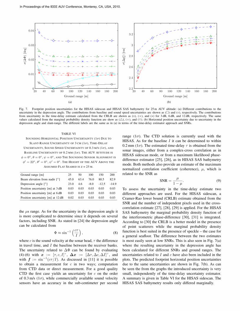
Fig. 7. Footprint position uncertainties for the HISAS sidescan and HISAS SAS bathymetry for 25 m AUV altitude: (a) Different contributions to theuncertainty in the depression angle. The contributions from baseline and sound speed uncertainties are shown as (�) and (◦), respectively. The contributionsfrom uncertainty in the time-delay estimate calculated from the CRLB are shown as (�), (×), and (∗) for 3 dB, 6 dB, and 12 dB, respectively. The samevalues calculated from the marginal probability density function are show as (4), (+), and (O). (b) Horizontal position uncertainty due to uncertainty in thedepression angle and slant-range. The different labels are the same as in (a) in terms of the time-delay estimator approach and SNRs.

TABLE VISOUNDING HORIZONTAL POSITION UNCERTAINTY (1σ) DUE TO

SLANT-RANGE UNCERTAINTY OF 3 CM (1σ), TIME-DELAY

UNCERTAINTY, SOUND SPEED UNCERTAINTY OF 0.3 M/S (1σ), AND

BASELINE UNCERTAINTY OF 0.2 MM (1σ). THE AUV ATTITUDE IS

φ = 0◦ , θ = 0◦ , ψ = 0◦ , AND THE SOUNDING SENSOR ALIGNMENT IS

φ′ = 22◦ , θ′ = 0◦ , ψ′ = 0◦ . THE HEIGHT OF THE AUV ABOVE THE

ASSUMED FLAT SEABED IS Z = 25 M.

Ground range [m] 25 50 100 150 200Beam elevation from nadir [◦] 45.0 63.4 76.0 80.5 82.9Depression angle [◦] 23.0 4.6 -8.0 -12.5 -14.9Position uncertainty [m] at 3 dB 0.03 0.03 0.03 0.03 0.03Position uncertainty [m] at 6 dB 0.03 0.03 0.03 0.03 0.03Position uncertainty [m] at 12 dB 0.02 0.03 0.03 0.03 0.03

the µs range. As for the uncertainty in the depression angle itis more complicated to determine since it depends on severalfactors, including SNR. As stated in [24] the depression anglecan be calculated from

Φ ≈ sin−1(cτI

), (8)

where c is the sound velocity at the sonar head, τ the differencein travel time, and I the baseline between the receiver banks.The uncertainty related to ∆Φ can be found by evaluating(4)-(6) with x := [τ, c, I]>, ∆x := [∆τ,∆c,∆I]>, andwith f := sin−1(cτ/I). As discussed in [11] it is possibleto obtain a measurement for c in two ways; computationfrom CTD data or direct measurement. For a good qualityCTD the first case yields an uncertainty for c on the orderof 0.3 m/s (1σ), while commercially available sound velocitysensors have an accuracy in the sub-centimeter per second

range (1σ). The CTD solution is currently used with theHISAS. As for the baseline I it can be determined to within0.2 mm (1σ). The estimated time-delay τ is obtained from thesonar images, either from a complex-cross correlation as inHISAS sidescan mode, or from a maximum likelihood phase-difference estimator [25], [26], as in HISAS SAS bathymetrymode. Both methods also provide an estimate of the maximumnormalized correlation coefficient (coherence), µ, which isrelated to the SNR as

SNR =µ

1− µ. (9)

To assess the uncertainty in the time-delay estimate twodifferent approaches are used. For the HISAS sidescan, aCramer-Rao lower bound (CRLB) estimate obtained from theSNR and the number of independent pixels used in the cross-correlation estimate [27], [28], [29] is applied. For the HISASSAS bathymetry the marginal probability density function ofthe interferometric phase-difference [30], [31] is integrated.According to [30] the CRLB is a better model in the presenceof point scatterers while the marginal probability densityfunction is best suited in the presence of speckle – the case fora general seafloor. The difference between the two estimatesis most easily seen at low SNRs. This is also seen in Fig. 7(a)where the resulting uncertainty in the depression angle hasbeen calculated for different SNRs and ground ranges. Theuncertainties related to I and c have also been included in theplots. The predicted footprint horizontal position uncertaintiesdue to the same uncertainties are shown in Fig. 7(b). As canbe seen the from the graphs the introduced uncertainty is verysmall, independently of the time-delay uncertainty estimator.A summary is given in Table VI for the HISAS sidescan. TheHISAS SAS bathymetry results only differed marginally.


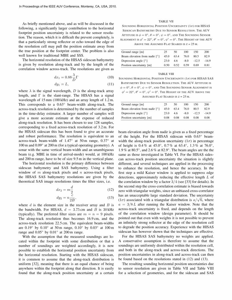
As briefly mentioned above, and as will be discussed in thefollowing, a significantly larger contribution to the horizontalfootprint position uncertainty is related to the sensor resolu-tion. The reason, which it is difficult the prevent completely, isthat a particularly strong reflector or echo toward the edge ofthe resolution cell may pull the position estimate away fromthe true position at the footprint center. The problem is alsowell known for traditional MBE and SSS.

The horizontal resolution of the HISAS sidescan bathymetryis given by resolution along-track and by the length of thecorrelation window across-track. The resolutions are given as

dx1 = 0.88λ

DΓ (10)

dy1 = L, (11)

where λ is the signal wavelength, D is the along-track arraylength, and Γ is the slant-range. The HISAS has a signalwavelength of 15 mm (100 kHz) and an array length of 1.2 m.This corresponds to a 0.63◦ beam-width along-track. Theacross-track resolution is determined by the number of samplesin the time-delay estimator. A larger number of samples willgive a more accurate estimate at the expense of reducedalong-track resolution. It has been chosen to use 128 samples,corresponding to a fixed across-track resolution of 3.2 m. Forthe HISAS sidescan this has been found to give an accurateand robust performance. The resolution is equivalent to anacross-track beam-width of 1.47◦ at 50 m range, 0.37◦ at100 m and 0.09◦ at 200 m (for a typical operating geometry). Asonar with the same vertical beam-width and an unambiguousbeam (e.g. MBE in time of arrival-mode) would, at 100 kHzand 200 m range, have to be of size 9.5 m in the vertical plane.

The horizontal resolution is the primary difference betweensidescan bathymetry and SAS bathymetry. Using a filterwindow of m along-track pixels and n across-track pixels,the HISAS SAS bathymetry resolutions are given by thetheoretical SAS image resolutions times the filter sizes, i.e.

dx2 = md

2(12)

dy2 = nc

2B, (13)

where d is the element size in the receiver array and B isthe bandwidth. For HISAS, d = 3.75 cm and B is 30 kHz(typically). The preferred filter sizes are m = n = 9 pixels.The along-track resolution thus becomes 16.9 cm, and theacross-track resolution 22.5 cm. The equivalent beam-widthsare 0.19◦ by 0.10◦ at 50 m range, 0.10◦ by 0.03◦ at 100 mrange and 0.05◦ by 0.01◦ at 200 m range.

With the assumption that the measured soundings are lo-cated within the footprint with some distribution or that anumber of soundings are weighted accordingly, it is nowpossible to establish the horizontal position uncertainty fromthe horizontal resolution. Starting with the HISAS sidescan,it is common to assume that the along-track distribution isuniform [32], meaning that there is an equal chance of beinganywhere within the footprint along that direction. It is easilyfound that the along-track position uncertainty at a certain

TABLE VIISOUNDING HORIZONTAL POSITION UNCERTAINTY (1σ) FOR HISASSIDESCAN BATHYMETRY DUE TO SENSOR RESOLUTION. THE AUV

ATTITUDE IS φ = 0◦ , θ = 0◦ , ψ = 0◦ , AND THE SOUNDING SENSOR

ALIGNMENT IS φ′ = 22◦ , θ′ = 0◦ , ψ′ = 0◦ . THE HEIGHT OF THE AUVABOVE THE ASSUMED FLAT SEABED IS Z = 25 M.

Ground range [m] 25 50 100 150 200Beam elevation from nadir [◦] 45.0 63.4 76.0 80.5 82.9Depression angle [◦] 23.0 4.6 -8.0 -12.5 -14.9Position uncertainty [m] 0.50 0.52 0.59 0.69 0.81

TABLE VIIISOUNDING HORIZONTAL POSITION UNCERTAINTY (1σ) FOR HISAS SAS

BATHYMETRY DUE TO SENSOR RESOLUTION. THE AUV ATTITUDE IS

φ = 0◦ , θ = 0◦ , ψ = 0◦ , AND THE SOUNDING SENSOR ALIGNMENT IS

φ′ = 22◦ , θ′ = 0◦ , ψ′ = 0◦ . THE HEIGHT OF THE AUV ABOVE THE


Ground range [m] 25 50 100 150 200Beam elevation from nadir [◦] 45.0 63.4 76.0 80.5 82.9Depression angle [◦] 23.0 4.6 -8.0 -12.5 -14.9Position uncertainty [m] 0.08 0.08 0.08 0.08 0.08

beam elevation angle from nadir is given as a fixed percentageof the height. For the HISAS sidescan with 0.63◦ beam-width the along-track position uncertainty (1σ) in percentageof height is 0.4 % at 45.0◦, 0.7 % at 63.4◦, 1.3 % at 76.0◦,1.9 % at 80.5◦, and 2.6 % at 82.9◦. The beam angles are the thesame as those investigated in Table VI. For the HISAS sides-can across-track position uncertainty the situation is slightlydifferent, and several techniques are applied in the processingto enhance the resolution, and hence the accuracy. In thefirst step a mild Kaiser window is applied to suppress edgedetections, approximately reducing the effective length L ofthe correlation window by a factor 3/4 (see [33] for details). Inthe second step the cross-correlation estimate is biased towardszero with triangular weights, since an unbiased cross-correlatorhas an unacceptable large standard deviation. The uncertainty(1σ) associated with a triangular distribution is a/

√6, where

a = 3/8L after running the Kaiser window. Note that theacross-track uncertainty is fixed, and depends on the lengthof the correlation window (design parameter). It should bepointed out that even with weights it is not possible to preventan infinitely strong reflector at the edge of the resolution cellto degrade the position accuracy. Experience with the HISASsidescan has however shown that the techniques are effective.

For the HISAS SAS bathymetry no weights are applied.A conservative assumption is therefore to assume that thesoundings are uniformly distritbuted within the resolution cell,and both in the along-track and across-track directions. Theposition uncertainties in along-track and across-track can thenbe found based on the resolutions stated in (12) and (13).

The resulting sounding horizontal position uncertainties dueto sensor resolution are given in Table VII and Table VIIIfor a selection of geometries, and for the sidescan and SAS


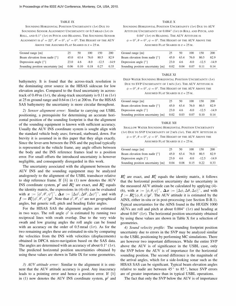
TABLE IXSOUNDING HORIZONTAL POSITION UNCERTAINTY (1σ) DUE TO

SOUNDING SENSOR ALIGNMENT UNCERTAINTY OF 0.5 MRAD (1σ) IN

ROLL, AND 0.1◦ (1σ) IN PITCH AND HEADING. THE SOUNDING SENSOR

ALIGNMENT IS φ′ = 22◦ , θ′ = 0◦ , ψ′ = 0◦ . THE HEIGHT OF THE AUVABOVE THE ASSUMED FLAT SEABED IS Z = 25 M.

Ground range [m] 25 50 100 150 200Beam elevation from nadir [◦] 45.0 63.4 76.0 80.5 82.9Depression angle [◦] 23.0 4.6 -8.0 -12.5 -14.9Sounding position uncertainty [m] 0.06 0.10 0.18 0.27 0.35

bathymetry. It is found that the across-track resolution isthe dominating error source in the HISAS sidescan for lowelevation angles. Compared to the fixed uncertainty in across-track of 0.49 m (1σ), the along-track uncertainty is 0.11 m (1σ)at 25 m ground range and 0.64 m (1σ) at 200 m. For the HISASSAS bathymetry the uncertainty is more circular throughout.

2) Sensor alignment error: Similar to carrying out USBLpositioning, a prerequisite for determining an accurate hori-zontal position of the sounding footprint is that the alignmentof the sounding equipment is known with sufficient accuracy.Usually the AUV INS coordinate system is sought align withthe standard vehicle body axes; forward, starboard, down. Forbrevity it is assumed in in this paper that they align exactly.Since the lever-arm between the INS and the payload typicallyis represented in the vehicle frame, any angle offsets betweenthe body and the INS reference frames lead to a positionerror. For small offsets the introduced uncertainty is howevernegligible, and consequently disregarded in this work.

The uncertainty associated with the alignment between theAUV INS and the sounding equipment may be analyzedanalogously to the alignment of the USBL transducer relativeto ship reference frame. If {b} in (1) now denotes the AUVINS coordinate system, pt and Rn

b are exact, and Rnb equals

the identity matrix, the expressions in (4)-(6) can be evaluatedwith x := [φ′, θ′, ψ′]>, ∆x := [∆φ′,∆θ′,∆ψ′]>, and withf := Rb

t(φ′, θ′, ψ′)pt. Note that φ′, θ′, ψ′ are not geographical

angles, but generic roll, pitch and heading Euler angles.For the HISAS SAS the alignment angles are estimated

in two ways. The roll angle φ′ is estimated by running tworeciprocal lines with swath overlap. Due to the very wideswath and low grazing angles the roll angle can be foundwith an accuracy on the order of 0.5 mrad (1σ). As for thetwo remaining angles these are estimated in-situ by comparingthe velocities from the INS with velocities (displacements)obtained in DPCA micro-navigation based on the SAS data.The angles are determined with an accuracy of about 0.1◦ (1σ).The predicted horizontal position uncertainties obtained byusing these values are shown in Table IX for some geometries.

3) AUV attitude error: Similar to the alignment it is emi-nent that the AUV attitude accuracy is good. Any inaccuracyleads to a pointing error and hence a position error. If {b}in (1) now denotes the AUV INS coordinate system, pt and

TABLE XSOUNDING HORIZONTAL POSITION UNCERTAINTY (1σ) DUE TO AUVATTITUDE UNCERTAINTY OF 0.004◦ (1σ) IN ROLL AND PITCH, AND

0.04◦ (1σ) IN HEADING. THE AUV ATTITUDE IS

φ = 0◦, θ = 0◦, ψ = 0◦ . THE HEIGHT OF THE AUV ABOVE THE



TABLE XIDEEP WATER SOUNDING HORIZONTAL POSITION UNCERTAINTY (1σ)DUE TO SVP UNCERTAINTY OF 1 M/S (1σ). THE AUV ATTITUDE IS




TABLE XIISHALLOW WATER SOUNDING HORIZONTAL POSITION UNCERTAINTY

(1σ) DUE TO SVP UNCERTAINTY OF 2 M/S (1σ). THE AUV ATTITUDE IS




Rbt are exact, and Rb

t equals the identity matrix, it followsthat the horizontal position uncertainty due to uncertainty inthe measured AUV attitude can be calculated by applying (4)-(6), with x := [φ, θ, ψ]>, ∆x := [∆φ,∆θ,∆ψ]>, and withf := Rn

b (φ, θ, ψ)pt. The AUV attitude it is estimated by theAINS, either in-situ or in post-processing (see Section II-B.1).Typical uncertainties for the AINS found in the HUGIN 1000AUVs are roll and pitch at about 0.004◦ (1σ) and heading atabout 0.04◦ (1σ). The horizontal position uncertainty obtainedby using these values are shown in Table X for a selection ofgeometries.

4) Sound velocity profile: The sounding footprint positionuncertainty due to errors in the SVP may be analyzed similarto the USBL positioning by performing MC simulations. Thereare however two important differences. While the entire SVPabove the AUV is of significance in the USBL case, onlythe SVP below the AUV is of importance for the horizontalsounding position. The second difference is the magnitude ofthe arrival angles, which for a side-looking sonar such as theHISAS SAS can be significant. Typical beam elevation anglesrelative to nadir are between 45 ◦ to 85 ◦, hence SVP errorsare of greater importance than in typical USBL operations.

The fact that only the SVP below the AUV is of importance


for the HISAS means that the performance typically will varymore in shallow than in deep waters. As mentioned, the SVPerror usually becomes smaller with depth, and consequentlyalso the SVP error of importance to the sounding equipment.As discussed, commercially available sound speed sensorsare available with an accuracy in the sub-centimeter persecond range (1σ), making the associate sounding uncertaintynegligible; independently of the beam elevation angle.

The effect of SVP errors are similar for the HISAS sidescanand HISAS SAS bathymetry. Two different cases are simu-lated, where one is for deep water, and one is for shallow water.The results are summarized in Table XI and Table XII. Only aconstant error model is applied in the deep water case, whilethe first order Gauss-Markov model is applied in addition tothe constant offset model in the shallow water case (the totalSVP uncertainty is evenly divided between the two models).

Finally note that work has been done where the error inthe SVP is estimated from overlapping MBE data [34], andconsequently reducing the position (and depth) error. Thetechnique may also be applied on HISAS sidescan and HISASSAS bathymetry data.

C. Other Error Sources

While the list of error sources discussed above is fairlyextensive, it is by no means complete. The need for accuratetiming has not been discussed, but it is clearly a prerequisite– both for synchronization of payload and AUV navigationdata, but also for synchronization of the AUV against thetopside clock connected to the USBL positioning. In theHUGIN AUVs the payload sensors and the navigation systemare synchronized against the same 1 PPS in-situ and willconsequently not drift relative to each other. Before launch theAUV is also synchronized to GPS, and consequently also theHiPAP system. Several types of crystal oscillators may be usedbut most are 1 ppm or better. For a mission lasting for 24 hthis corresponds to 86.4 ms. For an AUV traveling at 2 m/sforward speed this induces a 17 cm positioning error along-track. Oscillators with as low as 0.02 ppm drift are howeveravailable [18], making the problem negligible.

As for additional errors sources related to the soundingequipment one could mention contribution from 2pi wrappingand multipath. A further discussion is beyond the scope of thispaper. The reader is referred to [35] for a further discussion.

IV. DTM HORIZONTAL ERROR BUDGET

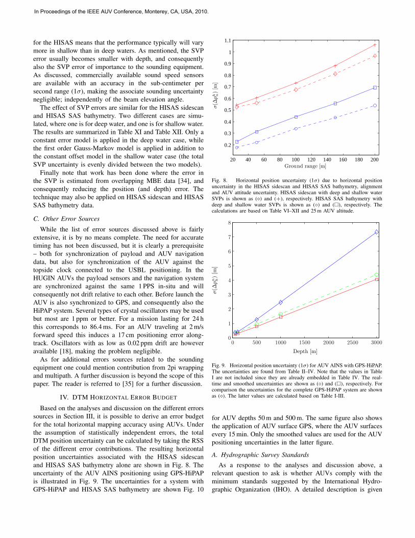
Based on the analyses and discussion on the different errorssources in Section III, it is possible to derive an error budgetfor the total horizontal mapping accuracy using AUVs. Underthe assumption of statistically independent errors, the totalDTM position uncertainty can be calculated by taking the RSSof the different error contributions. The resulting horizontalposition uncertainties associated with the HISAS sidescanand HISAS SAS bathymetry alone are shown in Fig. 8. Theuncertainty of the AUV AINS positioning using GPS-HiPAPis illustrated in Fig. 9. The uncertainties for a system withGPS-HiPAP and HISAS SAS bathymetry are shown Fig. 10

20 40 60 80 100 120 140 160 180 200

0.2

0.3

0.4

0.5

0.6

0.7

0.8

0.9

1

1.1

Ground range [m]

σ(∆

ph n)[m

]

Fig. 8. Horizontal position uncertainty (1σ) due to horizontal positionuncertainty in the HISAS sidescan and HISAS SAS bathymetry, alignmentand AUV attitude uncertainty. HISAS sidescan with deep and shallow waterSVPs is shown as (�) and (+), respectively. HISAS SAS bathymetry withdeep and shallow water SVPs is shown as (◦) and (�), respectively. Thecalculations are based on Table VI–XII and 25 m AUV altitude.

Depth [m]

σ(∆

pn h)[m

]

0 500 1000 1500 2000 2500 30000

1

2

3

4

5

6

7

8

Fig. 9. Horizontal position uncertainty (1σ) for AUV AINS with GPS-HiPAP.The uncertainties are found from Table II–IV. Note that the values in TableI are not included since they are already embedded in Table IV. The real-time and smoothed uncertainties are shown as (◦) and (�), respectively. Forcomparison the uncertainties for the complete GPS-HiPAP system are shownas (�). The latter values are calculated based on Table I-III.

for AUV depths 50 m and 500 m. The same figure also showsthe application of AUV surface GPS, where the AUV surfacesevery 15 min. Only the smoothed values are used for the AUVpositioning uncertainties in the latter figure.

A. Hydrographic Survey Standards

As a response to the analyses and discussion above, arelevant question to ask is whether AUVs comply with theminimum standards suggested by the International Hydro-graphic Organization (IHO). A detailed description is given


Ground range [m]

σ(∆

pn h)[m

]

20 40 60 80 100 120 140 160 180 2000.2

0.4

0.6

0.8

1

1.2

1.4

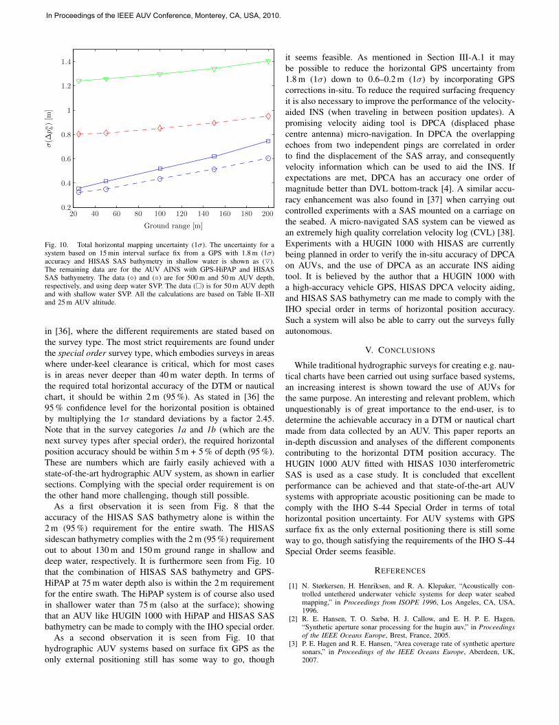
Fig. 10. Total horizontal mapping uncertainty (1σ). The uncertainty for asystem based on 15 min interval surface fix from a GPS with 1.8 m (1σ)accuracy and HISAS SAS bathymetry in shallow water is shown as (O).The remaining data are for the AUV AINS with GPS-HiPAP and HISASSAS bathymetry. The data (�) and (◦) are for 500 m and 50 m AUV depth,respectively, and using deep water SVP. The data (�) is for 50 m AUV depthand with shallow water SVP. All the calculations are based on Table II–XIIand 25 m AUV altitude.

in [36], where the different requirements are stated based onthe survey type. The most strict requirements are found underthe special order survey type, which embodies surveys in areaswhere under-keel clearance is critical, which for most casesis in areas never deeper than 40 m water depth. In terms ofthe required total horizontal accuracy of the DTM or nauticalchart, it should be within 2 m (95 %). As stated in [36] the95 % confidence level for the horizontal position is obtainedby multiplying the 1σ standard deviations by a factor 2.45.Note that in the survey categories 1a and 1b (which are thenext survey types after special order), the required horizontalposition accuracy should be within 5 m + 5 % of depth (95 %).These are numbers which are fairly easily achieved with astate-of-the-art hydrographic AUV system, as shown in earliersections. Complying with the special order requirement is onthe other hand more challenging, though still possible.

As a first observation it is seen from Fig. 8 that theaccuracy of the HISAS SAS bathymetry alone is within the2 m (95 %) requirement for the entire swath. The HISASsidescan bathymetry complies with the 2 m (95 %) requirementout to about 130 m and 150 m ground range in shallow anddeep water, respectively. It is furthermore seen from Fig. 10that the combination of HISAS SAS bathymetry and GPS-HiPAP at 75 m water depth also is within the 2 m requirementfor the entire swath. The HiPAP system is of course also usedin shallower water than 75 m (also at the surface); showingthat an AUV like HUGIN 1000 with HiPAP and HISAS SASbathymetry can be made to comply with the IHO special order.

As a second observation it is seen from Fig. 10 thathydrographic AUV systems based on surface fix GPS as theonly external positioning still has some way to go, though

it seems feasible. As mentioned in Section III-A.1 it maybe possible to reduce the horizontal GPS uncertainty from1.8 m (1σ) down to 0.6–0.2 m (1σ) by incorporating GPScorrections in-situ. To reduce the required surfacing frequencyit is also necessary to improve the performance of the velocity-aided INS (when traveling in between position updates). Apromising velocity aiding tool is DPCA (displaced phasecentre antenna) micro-navigation. In DPCA the overlappingechoes from two independent pings are correlated in orderto find the displacement of the SAS array, and consequentlyvelocity information which can be used to aid the INS. Ifexpectations are met, DPCA has an accuracy one order ofmagnitude better than DVL bottom-track [4]. A similar accu-racy enhancement was also found in [37] when carrying outcontrolled experiments with a SAS mounted on a carriage onthe seabed. A micro-navigated SAS system can be viewed asan extremely high quality correlation velocity log (CVL) [38].Experiments with a HUGIN 1000 with HISAS are currentlybeing planned in order to verify the in-situ accuracy of DPCAon AUVs, and the use of DPCA as an accurate INS aidingtool. It is believed by the author that a HUGIN 1000 witha high-accuracy vehicle GPS, HISAS DPCA velocity aiding,and HISAS SAS bathymetry can me made to comply with theIHO special order in terms of horizontal position accuracy.Such a system will also be able to carry out the surveys fullyautonomous.

V. CONCLUSIONS

While traditional hydrographic surveys for creating e.g. nau-tical charts have been carried out using surface based systems,an increasing interest is shown toward the use of AUVs forthe same purpose. An interesting and relevant problem, whichunquestionably is of great importance to the end-user, is todetermine the achievable accuracy in a DTM or nautical chartmade from data collected by an AUV. This paper reports anin-depth discussion and analyses of the different componentscontributing to the horizontal DTM position accuracy. TheHUGIN 1000 AUV fitted with HISAS 1030 interferometricSAS is used as a case study. It is concluded that excellentperformance can be achieved and that state-of-the-art AUVsystems with appropriate acoustic positioning can be made tocomply with the IHO S-44 Special Order in terms of totalhorizontal position uncertainty. For AUV systems with GPSsurface fix as the only external positioning there is still someway to go, though satisfying the requirements of the IHO S-44Special Order seems feasible.

REFERENCES

[1] N. Størkersen, H. Henriksen, and R. A. Klepaker, “Acoustically con-trolled untethered underwater vehicle systems for deep water seabedmapping,” in Proceedings from ISOPE 1996, Los Angeles, CA, USA,1996.

[2] R. E. Hansen, T. O. Sæbø, H. J. Callow, and E. H. P. E. Hagen,“Synthetic aperture sonar processing for the hugin auv,” in Proceedingsof the IEEE Oceans Europe, Brest, France, 2005.

[3] P. E. Hagen and R. E. Hansen, “Area coverage rate of synthetic aperturesonars,” in Proceedings of the IEEE Oceans Europe, Aberdeen, UK,2007.


[4] B. Jalving, K. Gade, O. Hagen, and K. Vestgard, “A toolbox of aidingtechniques for the HUGIN AUV integrated inertial navigation system,”in Proceedings of the MTS/IEEE Oceans Conference and Exhibition,San Diego, CA, 2003, pp. 1146–1153.

[5] P. E. Hagen, Ø. Hegrenæs, B. Jalving, Ø. Midtgaard, M. Wiig, and O. K.Hagen, “Making AUVs truly autonomous,” in Underwater Vehicles.Vienna, Austria: In-Tech Education and Publishing, January 2009.

[6] Øyvind Hegrenæs, “Autonomous navigation for underwater vehicles,”Ph.D. dissertation, Norwegian University of Science and Technology,2010.

[7] K. Gade, “NavLab, a generic simulation and post-processing tool fornavigation,” European Journal of Navigation, vol. 2, no. 4, pp. 21–59,Nov. 2004, (see also http://www.navlab.net/).

[8] A. B. Willumsen and Ø. Hegrenæs, “The joys of smoothing,” inProceedings of the IEEE Oceans Conference and Exhibition, Bremen,Germany, 2009.

[9] B. Jalving, K. Vestgard, and N. Størkersen, “Detailed seabed surveyswith AUVs,” in Technology and Applications of Autonomous Under-water Vehicles, G. Griffiths, Ed. Taylor & Francis, 2003, vol. 2, pp.179–201.

[10] R. M. Hare, “Depth and position error budgets for multi-beamechosounding,” in International Hydrographic Review, Monaco, 1995.

[11] B. Jalving, “Depth accuracy in seabed mapping with underwater ve-hicles,” in Proceedings of the MTS/IEEE Oceans Conference andExhibition, Seattle, WA, USA, 1999, pp. 973–978.

[12] J. G. Blackinton, “Bathymetric resolution, precision and accuracy con-siderations for swath bathymetry mapping sonar systems,” in Proceed-ings of the IEEE Oceans Conference and Exhibition, Honolulu, HI, USA,1991.

[13] S. B. Bisnath and Y. Gao, “Innovation: Precise point positioning - apowerful technique with a promising future,” GPS World, Apr. 2009.

[14] N. S. Kjørsvik and E. Brøste, “Using TerraPOS for efficient and accuratemarine positioning,” 2009.

[15] P. H. Milne, Underwater Acoustic Positioning Systems. Gulf PublishingCompany, 1983.

[16] K. Vickery, “Acoustic positioning systems. A practical overview of cur-rent systems,” in Proceedings of the Autonomous Underwater VehiclesWorkshop, Cambridge, MA, USA, 1998, pp. 5–17.

[17] Ø. Hegrenæs, K. Gade, O. K. Hagen, and P. E. Hagen, “Underwatertransponder positioning and navigation of autonomous underwater ve-hicles,” in Proceedings of the IEEE Oceans Conference and Exhibition,Biloxi, USA, Oct. 2009.

[18] R. M. Eustice, L. L. Whitcomb, H. Singh, and M. Grund, “Experimentalresults in synchronous-clock one-way-travel-time acoustic navigationfor autonomous underwater vehicles,” in Proceedings of the IEEEInternational Conference on Robotics and Automation (ICRA), Rome,Italy, Apr. 2007, pp. 4257–4264.

[19] S. E. Webster, R. M. Eustice, H. Singh, and L. L. Whitcomb, “Prelim-inary deep water results in single-beacon one-way-travel-time acousticnavigation for underwater vehicles,” in Proceedings of the IEEE/RSJInternational Conference on Intelligent Robots and Systems, St. Louis,MO, USA, Oct. 2009.

[20] T. I. Fossen, Marine Control Systems: Guidance, Navigation and Controlof Ships, Rigs and Underwater Vehicles. Marine Cybernetics, 2002.

[21] J. R. Taylor, An Introduction to Error Analysis: The Study of Uncertain-ties in Physical Measurements. University Science Books, 1996.

[22] A. Gelb, Applied Optimal Estimation. The MIT Press, 1974.[23] X. Lurton, An Introduction to Undewater Acoustics: Principles and

Applications. Springer-Praxis, 2002.[24] R. E. Hansen, T. O. Sæbø, K. Gade, and S. Chapman, “Signal processing

for AUV based interferometric synthetic aperture sonar,” in Proceedingsof the MTS/IEEE Oceans Conference and Exhibition, San Diego, CA,USA, 2003, pp. 2438–44.

[25] D. C. Ghiglia and M. D. Pritt, Two-Dimensional Phase Unwrapping:Theory, Algorithms, and Software. New York, NY, USA: John Wiley& Sons, INC, 1998.

[26] T. O. Sæbø, B. Langli, H. J. Callow, E. O. Hammerstad, and R. E.Hansen, “Bathymetric capabilities of the HISAS interferometric syn-thetic aperture sonar,” in Proceedings of the MTS/IEEE Oceans Confer-ence and Exhibition, Vancouver, Canada, October 2007.

[27] A. H. Quazi, “An overview on the time delay estimate in active andpassive systems for target localization,” IEEE Transactions on Acoustics,Speech and Signal Processing, vol. ASSP-29, no. 3, pp. 527–533, 1981.

[28] A. Bellettini and M. A. Pinto, “Theoretical accuracy of synthetic aperturesonar micronavigation using a displaced phase-center antenna,” IEEEJournal of Oceanic Engineering, vol. 27, no. 4, pp. 780–789, 2002.

[29] T. O. Sæbø, R. E. Hansen, and A. Hanssen, “Relative height estimationby cross-correlating ground-range synthetic aperture sonar images,”IEEE Journal of Oceanic Engineering, vol. 32, no. 4, pp. 971–982,October 2007.

[30] R. F. Hanssen, Radar Interferometry: Data Interpretation and ErrorAnalysis. Dordrecht, The Netherlands: Kluwer Academic Publishers,2001.

[31] G. Franceschetti and R. Lanari, Synthetic Aperture Radar Processing.Boca Raton, FL, USA: CRC Press, 1999.

[32] E. Hammerstad, “Multibeam echo sounder accuracy,” Kongsberg Sim-rad, Horten, Norway, EM Technical Note, 1998.

[33] H. L. Van Trees, Optimum array processing. Part IV of detection,estimation, and modulation theory. New York, USA: John Wiley &Sons Inc., 2002.

[34] M. Snellen, K. Siemes, and D. G. Simons, “An efficient method forreducing the sound speed induced errors in multibeam echosounderbathymetric measurements,” in Proceedings of Underwater AcousticsMeasurements, Nafplion, Greece, 2009.

[35] P. N. Denbigh, “Swath bathymetry: principles of operation and ananalysis of errors,” IEEE Journal of Oceanic Engineering, vol. 14, no. 4,pp. 289–98, Oct. 1989.

[36] International Hydrographic Organization. IHO standards forhydrographic surveys, 5th edition. Accessed on April 20, 2010.[Online]. Available: http://www.iho-ohi.net

[37] K. Gade, “Aiding inertial navigation with DPCA micronavigation,” in6th Mine Detection & Classification Joint Research Program Meeting,NATO Undersea Research Centre, La Spezia, Italy, Nov. 2001.

[38] P. E. Hagen, R. E. Hansen, K. Gade, and E. Hammerstad, “Interfer-ometric synthetic aperture sonar for AUV based mine hunting: TheSENSOTEK project,” in Proceedings of Unmanned Systems, Baltimore,MD, USA, 2001.


horizontal mapping accuracy in hydrographic auv surveys

Documents