gary froyland, in alistair mees, editor, nonlinear dynamics and

Extracting dynamical behaviour via Markov models

Gary Froyland�

Abstract

Statistical properties of chaotic dynamical systems are di�cult to estimate reliably�Using long trajectories as data sets sometimes produces misleading results� It has beenrecognised for some time that statistical properties are often stable under the additionof a small amount of noise� Rather than analysing the dynamical system directly� weslightly perturb it to create a Markov model� The analogous statistical properties of theMarkov model often have �closed forms� and are easily computed numerically� TheMarkov construction is observed to provide extremely robust estimates and has thetheoretical advantage of allowing one to prove convergence in the noise� � limit andproduce rigorous error bounds for statistical quantities� We review the latest resultsand techniques in this area�

Contents

� Introduction and basic constructions �

�� What do we do� � � � � � � � � � � � � � � � � � � � � � � � � � � � � � � � � � � � �� How do we do this� � � � � � � � � � � � � � � � � � � � � � � � � � � � � � � � � � � �� Why do we do this� � � � � � � � � � � � � � � � � � � � � � � � � � � � � � � � � � �

� Objects and behaviour of interest �

�� Invariant measures � � � � � � � � � � � � � � � � � � � � � � � � � � � � � � � � � � �� Invariant sets � � � � � � � � � � � � � � � � � � � � � � � � � � � � � � � � � � � � � �� Decay of correlations � � � � � � � � � � � � � � � � � � � � � � � � � � � � � � � � � �� Lyapunov exponents � � � � � � � � � � � � � � � � � � � � � � � � � � � � � � � � � �� Mean and variance of return times � � � � � � � � � � � � � � � � � � � � � � � � � �

� Deterministic systems �

�� Basic constructions � � � � � � � � � � � � � � � � � � � � � � � � � � � � � � � � � � �� Invariant measures and invariant sets � � � � � � � � � � � � � � � � � � � � � � � � �� Decay of correlations and spectral approximation � � � � � � � � � � � � � � � � � �� Lyapunov exponents and entropy � � � � � � � � � � � � � � � � � � � � � � � � � � �� Mean and variance of return times � � � � � � � � � � � � � � � � � � � � � � � � � ��

� Random Systems ��

�� Basic constructions � � � � � � � � � � � � � � � � � � � � � � � � � � � � � � � � � � �� Invariant measures � � � � � � � � � � � � � � � � � � � � � � � � � � � � � � � � � � �� Lyapunov exponents � � � � � � � � � � � � � � � � � � � � � � � � � � � � � � � � � �� Mean and variance of return times � � � � � � � � � � � � � � � � � � � � � � � � � �� Advantages for Markov modelling of random dynamical systems � � � � � � � � �

� Miscellany ��

� Numerical Tips and Tricks �

�� Transition matrix construction � � � � � � � � � � � � � � � � � � � � � � � � � � � �� Partition selection � � � � � � � � � � � � � � � � � � � � � � � � � � � � � � � � � � ��

�Research supported by the Deutsche Forschungsgemeinschaft under Grant De ��

�

� Froyland

� Introduction and basic constructions

Suppose that we �nd ourselves presented with a discrete time� dynamical system� and wewould like to perform some �mainly ergodic�theoretic� analysis of the dynamics� We are notconcerned with the problem of embedding� nor with the extraction of a system from timeseries� We assume that we have been presented with a dynamical system and do not questionits validity�

Any analysis of a dynamical system involving average quantities requires a referencemeasure with which to average contributions from dierent regions of phase space� Oftenthe measure that one wishes to use is the probability measure that is described by thedistribution of a typical long trajectory of the system it is commonly called the natural

measure or physical measure of the system�

�� What do we do�

This chapter discusses a method of modelling the dynamics by a �nite state Markov chain�Naturally such a model contains much less information than the original dynamical system�However� this simpli�cation of the dynamics allows the exact computation of many propertiesof the Markov chain which correspond to important indicators and properties of the originaldynamics� For example� �nding invariant sets� obtaining invariant measures� calculatingrates of mixing and the spectrum of eigenvalues of transfer operators� computing means andvariances of recurrence times� and estimating Lyapunov exponents all of these calculationsare exact� for the Markov chain� We hope that although we are throwing away a lot ofinformation in our Markov model� we retain the essential properties of the original system�The questions then are� �i� Are these quantities computed for the Markov model goodestimators of the corresponding quantities for the original system� and �ii� how best tode�ne these Markov models for various sorts of systems�

�� How do we do this�

We describe the fundamental construction of the modelling process� Consider a dynamicalsystem �M�T � de�ned by a map T � M �

�

�� where M is a compact subset of Rd� Partitionthe phase space into a �nite number of connected sets fA�� Ang with nonempty interior�Usually� this partition will take the form of a regular grid covering the phase space M � Wenow completely ignore any dynamics that occurs inside each individual partition set� andfocus only on the coarse�grained dynamics displayed by the evolution of whole partition sets�To form our Markov model� we identify each set Ai with a state i of our n�state Markovchain� We construct an n� n transition matrix P � where the entry Pij is to be interpretedas�

Pij � the probability that a typical point in Ai moves into Aj under one iteration of the map T � ��

We now meet the notion of typicality and begin to impinge on ergodic�theoretic ideas� Leav�ing formality for the moment� we shall assume that the trajectories fx� Tx� T �x� � � �g ofLebesgue almost all initial points x �M have the same distribution on M � This distributionmay be represented as a probability measure� denoted by �� Now� in light of �� the most

�Similar constructions for �ows are possible by considering the �time�t� map��A further approximation must be introduced for the calculation of Lyapunov exponents�


natural de�nition of Pij is

�Pij ��Ai � T��Aj�

��Ai��

since �Pij � Prob�fTx � Ajjx � Aig� Unfortunately� the natural measure � is usuallyunknown and for want of a better alternative� we compute a �slightly� dierent transitionmatrix using normalised Lebesgue measure m instead of ��

Pij �m�Ai � T��Aj�

m�Ai��

Several numerical techniques have been put forward regarding the computation of P seex��

�� Why do we do this�

The alternative to Markov modelling of the dynamics via some coarse graining is to simplysimulate very long orbits of the dynamical system� For the purposes of this discussion� werestrict ourselves to the problem of approximating the probability measure � that describesthe asymptotic distribution of almost all trajectories�

Given a long orbit fx� Tx� � � � � TN��xg� one is implicitly approximating the long�termdistribution � by the �nite�time distribution �N�x� ��

�N

PN��k�� T kx� where �x is the delta�

measure at x � M � This is certainly a simple way to compute an approximate invariantmeasure �or long�term distribution�� as it does not involve any complicated matrix construc�tions one just iterates one�s map� There are however� drawbacks to this simple approach�It is possible that orbits display transient �non�equilibrium� behaviour for lengthy periodsof time before settling into a more regular �statistically speaking� mode� Thus� by followinga simulated orbit for a �nite time� there is the risk that one is only observing this transientbehaviour and not the true asymptotic behaviour of the system� There is also the problemof computer round�o try to �nd the long�term distribution of the tent map or the circledoubling map by iterative simulation �all trajectories are attracted to � in �nite time�� Theseare extreme cases� but the potential compounding inaccuracy of long computer generatedorbits should not be forgotten� Let�s be generous though� and assume that our approxima�tion �N�x� actually does �weakly� converge to �� How fast does this happen� What is theconvergence rate with respect to the length of the orbit N� Can one produce rigorous errorbounds for the dierence between the distributions �N�x� and �� For the most part� theanswer to each of these questions is �We don�t know yet�� In toy cases� one can produceextremely crude probabilistic lower bounds for the error� of the form C�

pN � but this is not

really satisfactory�Our method of Markov modelling attempts to overcome all of these di�culties� Transient

eects are completely removed as we model the system as a Markov chain and its asymptoticbehaviour may be computed exactly� Computer roundo is not so much of a problem� aswe are now only computing a single iterate of the dynamics rather than a compoundingsequence of iterations� The constructions also permit a rigorous treatment of questions likerates of convergence� error bounds� and even just whether convergence occurs at all� Finally�from the practical point of view� the method of Markov coarse graining is often very e�cientcomputationally� producing better answers in less time�

This discussion has primarily been aimed at the computation of invariant measures� butit applies also to the computation of other dynamical indicators such as the rate of decay

� Froyland

of correlations� Lyapunov exponents� and statistics of recurrence times� The rate of decayof correlations and the isolated spectrum of transfer operators in particular are notoriouslydi�cult to estimate via iterative techniques�

� Objects and behaviour of interest

In this section we give a summary of the de�nitions and properties of the objects we wishto estimate� Additional applications are outlined in x��

�� Invariant measures

The fundamental object for ergodic�theoretic concepts is an ergodic invariant probability

measure �� One should think of ��B� as representing the proportion of �mass� that iscontained in the subset B � M � The invariance condition of � is � � � � T�� This is ageneralised �conservation of mass� equality the mass distribution described by � is preservedunder the action of T � in the same way that area preserving maps preserve Lebesgue measure�Ergodicity is the measure�theoretic equivalent of topological transitivity� If two sets A andB both have positive ��measure� then there is an N � � such that ��A � T�NB� � � inother words� any region of positive ��mass may be evolved forward to intersect any otherregion of positive ��mass� with the intersection also having positive mass� Ergodic systemsare indecomposable in the sense that ��almost all starting points produce orbits with thesame asymptotic distribution� The Birkho theorem �� tells us that the frequency withwhich orbits of ��almost all starting points visit a set B is equal to the ��measure of Bformally�

limN��

��N��f� � k � N � � T kx � Bg � ��B� ��

for ��almost all x � M � However� as in the case of dissipative systems� there may be athin invariant attracting set � with �� but m�� Equation �� gives us noinformation about orbits starting o this invariant set�

De�nition �� An ergodic invariant probability measure is called a natural or physical

measure� if

limN��

�

N

N��Xk��

f�T kx�ZM

fd� ��

for all continuous f � M R and Lebesgue�almost all x � M �

An alternative way of phrasing the de�nition of a physical measure is to state that themeasure �N�x� of x�� converges weakly to � as N � for Lebesgue almost all x � M �When talking about physical measures� equation �� may be strengthened to�

Corollary ��

limN��

�

N�f� � k � N � � T kx � Bg � ��B� ��

for any subset B �M with ��B� � �� and for Lebesgue almost all x �M �

Extracting dynamical behaviour via Markov models �

Corollary �� says that �randomly chosen� initial conditions will with probability one�produce trajectories that distribute themselves according to the natural measure �� De�terministic chaotic systems typically have in�nitely many ergodic invariant measures �forexample� a convex combination of � measures on a periodic orbit�� but only one physicalmeasure�

Example �� The linear mapping of the torus T � T� �

�

� de�ned by T �x� y� � ��x �y� x � y� �mod �� has in�nitely many ergodic invariant measures� For example� �� andm � Lebesgue measure� Of all the ergodic invariant probability measures� only m satis�es��

�� Invariant sets

We approach invariant sets in a rather roundabout way� as we will describe them as thesupport of the physical measure� supp �� where supp � is the smallest closed set having �measure of � �equivalently� x � supp� i every open neighbourhood of x has positive �measure�� It is easy to show that T �supp�� supp � and supp � � T��supp��

The reason for choosing supp � as the distinguished invariant set� rather than someinvariant set de�ned via topological conditions is as follows� Let x be an arbitrary point insupp �� and B��x� be an open neighbourhood of size about x� By �� orbits of Lebesguealmost all initial points visit B��x� in�nitely often and with a positive frequency of visitation�Meanwhile regions away from supp� are visited with frequency �� As we wish to �ndthe invariant set which appears on computer simulations of trajectories� it makes sense toconsider only the support of � and not some larger topologically invariant set�

�� Decay of correlations

The measure�theoretic analogy of topological mixing is �measure�theoretic� mixing� We saythat a system �T� �� is mixing if ��A � T�NB� ��A��B� as N � for any pair ofmeasurable subsets A�B � M � This condition says that the probability that a point x liesin a set B at time t � � and then moves to a set A at time t � N �for large N� is roughly theproduct of the measures of the sets A and B� That is� for large N � the two events fx � Bgand fTNx � Ag become statistically independent� or decorrelated� For dynamical systemswith some degree of smoothness� this loss of dependence is often studied via the formula�

Cf�g�N� ��

��Z

f � TN � g d�Z

f d� �Z

g d�

��

where f � L��M�m� and g � M R has some smoothness properties� If one thinks ofthe functions f� g � M R as �physical observables� �output functions giving numericalinformation on some physical quantities of the system�� then Cf�g�N� quanti�es the corre�lation between observing g at time t and f at time t � N � If f � g� we obtain what iscommonly known as the autocorrelation function� For many chaotic systems� it is observedthat Cf�g�N� � at a geometric rate� and it is of interest to estimate this rate� The rateof decay can be interpreted variously as providing information on how quickly the systemsettles into statistically regular behaviour� how quickly transient behaviour disappears� andhow quickly physical observables become decorrelated� For all of these interpretations� thephysical measure � is central as it provides the reference measure that describes statisticalequilibrium for the system� Correlation decay has strong connections with transfer operators

�or Perron�Frobenius operators� and the spectrum and corresponding eigenfunctions of theseoperators� We postpone further discussion of these objects until x � �

� Froyland

�� Lyapunov exponents

The Lyapunov exponents of a �piecewise dierentiable� dynamical system describe the av�erage local rates of expansion and contraction in phase space that are felt along typicaltrajectories� We may de�ne them as the various values of that are observed� in the follow�ing expression� as v is varied over Rd

�� limN��

�

Nlog kDxT

N�v�k ��

As our dynamical system satis�es equation �� it is immediate that Lebesgue almost alltrajectories will produce the same d values of � and these values will be called the� Lyapunovexponents of T �

Later we will be discussing Lyapunov exponents of random matrix products� These canbe de�ned in an analogous way�

�� Mean and variance of return times

The statistics of return times of orbits to subsets of phase space have not received a greatdeal of attention in the dynamical systems literature� A recent exception is �� whereregularity properties of return times are used to prove existence of physical measures andcharacterise rates of decay of correlations as exponential or algebraic� Suppose that oneis given a subset B � M with ��B� � �� Every time a typical trajectory enters B� wenote down the number of iterations since the orbit last entered B� In this way� we obtaina sequence of times t�� t�� such that T tix � B� i � �� We may now ask what is themean and variance of this sequence of times� Formally� we de�ne a function R � M Z

by R�x� � inffk � � � T kx � Bg� and use this return time function to de�ne an inducedmap �Tx � TR�x�x� where �T � B �

�

�� It is straightforward to show that �jB �de�ned by�jB�C� � ��C��B� for C � B� is �T �invariant� Therefore� we can de�ne the mean returntime

E�jB�R� �

ZB

R�x� d�jB�x��

and the variance of the return times as

var�jB�R� � E�jB�R��E�jB�R�

��

By Kac�s theorem � �� E�jB�R� � ��B� provided � is ergodic� A corresponding simpleformula for the variance is not known�

� Deterministic systems

In the �rst of two parts� we focus on deterministic systems� We show how each of the objectsoutlined in x� will be approximated using the Markov model� We begin each subsection bysimply outlining the constructions and the computations one performs in practice� At theend of each subsection� we state situations where rigorous results are obtained� While theMarkov systems appear to retain many of the salient features of the original system� thesmooth dynamics is completely lost and so it is not at all straightforward to prove strongapproximation results�

�For a d�dimensional system� � may only take on at most d di�erent values��Lyapunov exponents depend very much on a reference measure �in this case the physical measure� in

order to be de�ned�


�� Basic constructions

The region M is covered with a collection of connected sets Pn � fAn�� An�ng withnonempty interiors� This covering has the properties that �i�

Sni��An�i � M and �ii� IntAn�i�

IntAn�j � for i �� j� where IntA denotes the interior of A� We think of each Ai as being aclosed set� so that we do not have a partition in the strict sense� as the sets in the coveringshare boundaries�

We construct the matrix

Pn�ij �m�An�i � T��An�j�

m�An�i�

as in � ��Clearly� the quality of our Markov model depends heavily on the choice of partition�

And it stands to reason that �ner partitions produce better models �this will soon be mademore precise�� We will frequently produce a sequence of Markov models� each constructedfrom successively �ner partitions� until we are satis�ed with the accuracy of the estimatesproduced by the model� Sometimes one can produce better models by clever re�nementstrategies these are discussed in x��

�� Invariant measures and invariant sets

Rough Idea� The invariant density of the Markov chain approximates the physical invariantmeasure of T �Required Computation� Calculate the �xed left eigenvector of P �

We �x our partition fAn�� An�ng and calculate Pn and pn� normalising pn so thatPni�� pn�i � �� The value pn�i is the weight given to state i by the stationary distribution

of the Markov chain� Since state i represents the set An�i in our smooth space� we de�nean approximate invariant measure �n by assigning �n�An�i� � pn�i� Within the set An�i� wedistribute the mass in any way we like� A common method is simply to spread the weightpn�i uniformly over An�i� so that formally�

�n�B� ��nXi��

�n�An�i�m�An�i � B�

m�An�i��

As we increase the number of partition sets n through re�nement� some of these re�nedsets will be given zero measure by �n as an indication that trajectories spend no time oralmost no time in these regions� Thus we expect that supp �n� � supp �n for n� � n �thiscan be made rigorous if T is a topological attractor ��

Further� since M is compact� the space of Borel probability measures on M �denotedM�M�� is compact with respect to the weak topology� We may therefore continue thisre�nement procedure �forever� and extract a limiting measure �� as

�� limn��

�n� ��

taking a convergent subsequence if necessary to de�ne the limit� It is always assumed thatmax��i�n diamAn�i ��

We have the following results concerning these approximations�

�This construction is often called Ulam�s method as it was �rst proposed in �� to use the matrix Pn toapproximate invariant densities of interval maps�

� Froyland

Theorem �� Suppose that T � M �

�

� is continuous and has a physical measure �� Let �ndenote the approximate invariant measures and �� a weak limit of this sequence� Denote byS the intersection

T�n�n�

supp �n� Then

�i� �� is T �invariant�

�ii� supp �� supp �n for all n � �� and therefore supp�� S�

�iii� supp � � supp �n for all n � �� and therefore supp � � S�

Proof�

�i� By noticing that the Markov models are small random perturbations � �� of T � itis relatively simple to prove that �� is T �invariant ��

�ii� This is a straightforward consequence of weak convergence�

�iii� This is proven in ��

�

The �rst result of Theorem �� says that weak limits of the sequence of numericallycomputed measures �n are T �invariant� In other words� we are in fact approximating some

T �invariant probability measure� However� there is the question of just which invariantmeasure this is� as �� may be distinct from �� the physical measure we wish to approximate�In this very general formulation� it is �as yet�� not possible to say that ��

Parts �ii� and �iii� of Theorem �� say that at least the supports of the computed measures�n do contain the supports of both �� and �� so that by stopping our computation at some�nite n� we are not �losing� regions that are given positive measure by the physical measure��

Example �� The stiletto map� We introduce the Stiletto map �� T � R� �

�

��

T �x� y� � ��x� �� exp� x � �� y� x��

This map seems to possess chaotic dynamics on a fractal attracting set see Figure �� Byselecting M � R

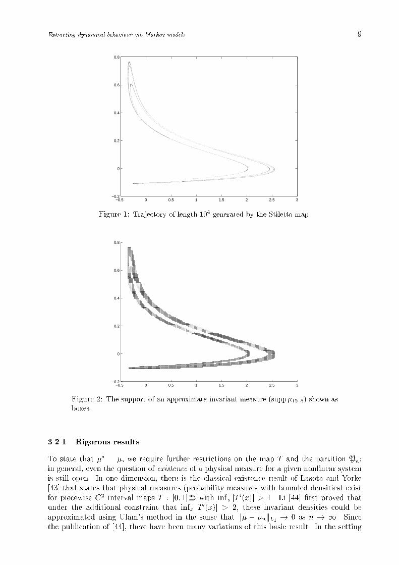
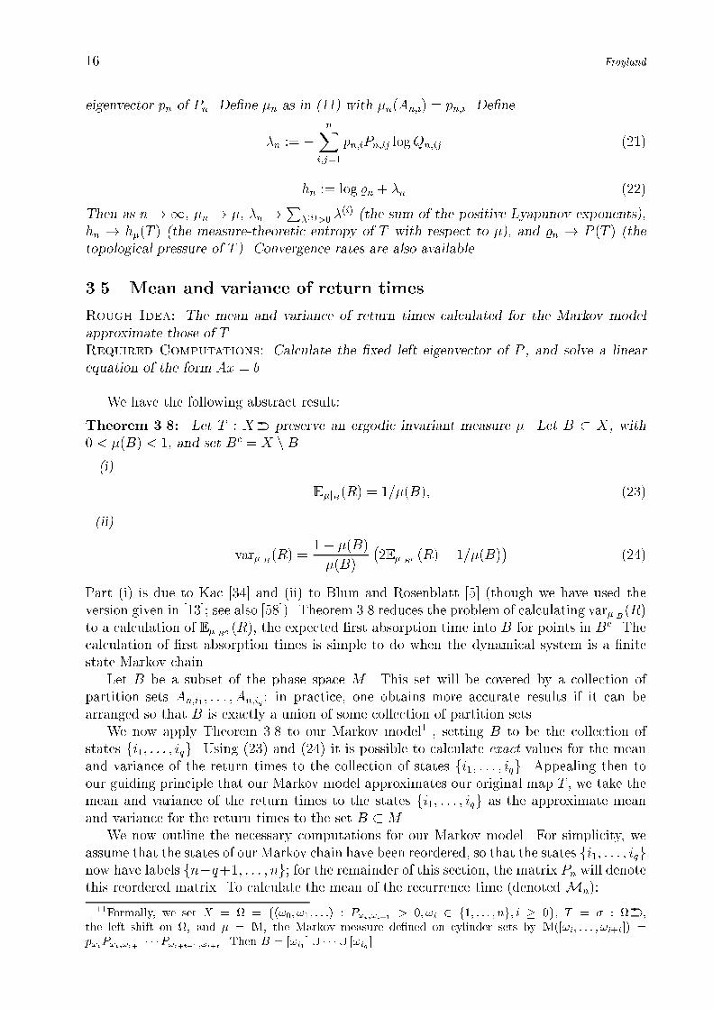
� to be a su�ciently small neighbourhood of the observed attracting set�it numerically appears that Lebesgue almost all x � M exhibit the invariant distributiondescribed by the density of points in Figure �� It is assumed that this distribution of points�in the in�nite limit� describes the physical measure �� We construct a Markov model using�� partition sets� where the sets are rectangles of equal size� The support of the resultingapproximate invariant measure is shown in Figure �� and the approximation itself is shownin Figure � We have used a relatively low number of partition sets for ease of viewing�Even for this crude model� there is good agreement between the distributions in Figures �and �

�A sign which may be taken as promise� or simply a state of ignorance� is that the author does notknow of a continuous dynamical system T with physical measure � for which �� using reasonably�regular� partitions and re�nements which keep the partition sets as approximate d�dimensional �cubes� ofapproximately the same shape and size��


−0.5 0 0.5 1 1.5 2 2.5 3−0.2

0

0.2

0.4

0.6

0.8

Figure �� Trajectory of length �� generated by the Stiletto map�

−0.5 0 0.5 1 1.5 2 2.5 3−0.2

0

0.2

0.4

0.6

0.8

Figure �� The support of an approximate invariant measure supp�� shown asboxes�

�� Rigorous results

To state that �� we require further restrictions on the map T and the partition Pnin general� even the question of existence of a physical measure for a given nonlinear systemis still open� In one dimension� there is the classical existence result of Lasota and Yorke�� that states that physical measures �probability measures with bounded densities� existfor piecewise C� interval maps T � ��

�

� with infx jT ��x�j � �� Li �� rst proved thatunder the additional constraint that infx jT ��x�j � �� these invariant densities could beapproximated using Ulam�s method in the sense that k� �nkL� � as n �� Sincethe publication of �� there have been many variations of this basic result� In the setting

�� Froyland

−0.5 0 0.5 1 1.5 2 2.5 3−0.2

0

0.2

0.4

0.6

0.8

Figure � Representation of an approximate invariant physical measure ��for the Stiletto map� Darker regions indicate higher density and more mass�

of �� Keller � �� proved k� �nkL� � O�logn�n�� Recent results �often under additional�ontoness� assumptions� have focussed on explicit error bounds for the dierence k��nkL� � ��

For higher dimensional uniformly expanding systems� very roughly speaking� the paperof Boyarsky and Gora �� and Ding �� mirror those of �� and �� There are severaladditional technical constraints on the map T and the partitions Pn that we do not discuss�Again under some ontoness conditions� Murray �� applies the methods of �� to provideerror bounds for k� �nkL� �

For uniformly hyperbolic systems� the author �� shows that �n � weakly �resp�in L�� when the physical measure � is singular �resp� absolutely continuous�� provided thatthe partitions Pn are Markov partitions�

A combination of theory and numerics �� suggests that the convergence rate O�logn�n�holds in reasonable generality for systems with good mixing properties�

�� Decay of correlations and spectral approximation

Rough Idea� The spectrum of the matrix P approximates the spectrum of the Perron�Frobenius operator�Required Computation� Calculate the eigenvalues of P �

We begin by noting that we have an alternative formulation of �� in terms of the Perron�Frobenius operator� P � L��M�m� �

�

��

Lemma �� Let F be a class of real�valued functions preserved by P� Let ��P� denote thespectrum of P when considered as an operator on F � and set r � supfjzj � z � ��P� n f�gg�Then there is a constant C �� such that Cf�g�N� � CrN if g � F and f � L��

�See �� for de�nitions and properties of the Perron�Frobenius operator��For example� if T is C� � then C��M�R� is preserved by P � and if T � ��

�

�

�

is a Lasota�Yorke map�then functions of bounded variation are preserved by P �

Extracting dynamical behaviour via Markov models ��

This result says that we may bound the rate of decay of correlations by the maximal non�unitspectral value for the operator P see Figure � �upper right� for the typical spectral plot wehave in mind� The Ulam matrix Pn may be thought of as a projection of P onto a �nitedimensional space� Naively� then� we may think that the spectrum of the matrix Pn willapproximate the spectrum of the Perron�Frobenius operator� This would be very useful� asit is simple to compute the spectrum of Pn since the matrix is very sparse and there arenumerical routines to compute only eigenvalues which are large in magnitude �these are theones that are principally of interest�� Furthermore� the eigenfunctions of P correspondingto large eigenvalues are also of interest� as they indicate the sorts of mass distributionsthat approach the equilibrium distribution �the physical measure� at the slowest possiblerate� Perhaps we can also approximate these slowly mixing distributions �eigenfunctions ofP� as eigenvectors of the matrix P � If we can� there is the question of what these slowlymixing distributions represent� One generally thinks that the rate of mixing is determinedby expansion properties of the dynamical system that is� the more expansive �or more�chaotic�� the greater the rate of decay� But the existence of distributions which mix ata rate slower than that dictated by the minimal expansion rate of the system� presents aseemingly paradoxical situation� Arguments in �� suggest that these distributionsdescribe �macroscopic structures� embedded within the dynamics� which exchange massvery slowly and work against the chaoticity�


There are two situations where these ideas can be made rigorous� First� for one�dimensionalmaps� there is the recent result of Keller and Liverani � ��

Theorem �� Let BV denote the space of functions of bounded variation on �� Sup�pose T � ��

�

� is an expanding� piecewise C� interval map� with infx�� jT ��x�j � � ��Then isolated eigenvalues of P � BV �

�

� outside the disk fjzj � �� g and the correspond�ing eigenfunctions are approximated by eigenvalues and the corresponding eigenvectors ofPn �eigenfunction convergence in the L� sense�� The convergence rate for the eigenvectorsto the eigenfunctions for eigenvalues z � � � �� is O�n�r�� where � � r�z� � �� while theeigenvector approximating the invariant density �z � �� converges like O�logn�n��

Example �� The double wigwam map� We introduce the map T � ��

�

� de�nedby

T �x� �

��

�x � � sin��x�� x � ��

�x �� sin��x �� x � ��

�x �� sin��x �� x � ��

��x �� sin�� x � �

�

the graph of which is shown in the upper left frame of Figure �� Theorem �� will be used toshow that the spectrum of P � BV �

�

� contains a non�trivial isolated eigenvalue� and thereforea rate of decay slower than that prescribed by the minimal expansion rate� As T is a Lasota�

Yorkemap� the classical result of �� tells us that T possesses an invariant density �this is thedensity of the physical measure�� The result of Li �� tells us that this invariant density maybe approximated by eigenvectors of the Ulam matrices� The bottom left frame of Figure �shows a plot of an approximation of the invariant density using an equipartition of �� into�� sets� The upper right frame shows the spectrum of the resulting �� matrix� Thelarge dotted circle denotes fjzj � �g� and the dash�dot inner circle shows the upper bound

�� Froyland

for the essential spectral radius for this map fjzj � �� g� �� infx�� jT ��x�j�The cross shows an eigenvalue of P�� that is clearly outside this inner region and thereforecorresponds to a true isolated eigenvalue of P� The eigenfunction for this isolated eigenvalueis plotted in the lower right frame�

−1 −0.5 0 0.5 1−1

−0.5

0

0.5

1Approximate spectrum

real part

imag

inar

y pa

rt

0 0.5 10

0.2

0.4

0.6

0.8

1The double wigwam map

x

Tx

0 0.2 0.4 0.6 0.8 10

0.5

1

1.5Invariant density

x0 0.2 0.4 0.6 0.8 1

−2

−1

0

1

2Eigenfunction for second eigenvalue

x

Figure �� upper left� Graph of T � upper right� Spectrum of �� transitionmatrix P�� the small circle represents the eigenvalue �� the small cross representsanother isolated eigenvalue� lower left� Plot of the invariant density of T theeigenfunction for the eigenvalue �� lower right� Plot of the eigenfunction for thesecond isolated eigenvalue�

What about higher�dimensional systems� For uniformly hyperbolic systems� a standardtechnique is to factor out the stable directions and consider only the action of T alongunstable manifolds W u� This induces an expanding map TE � W u �

�

� with correspondingPerron�Frobenius operator PE� We have the following result�

Theorem �� Let T � M �

�

� be C�� uniformly hyperbolic� and possessa nice� Markov partition� Construct Pn by setting Pn to be a re�nement of this Markovpartition� and consider PE to act on the function space C��W u�R�� Isolated eigenvaluesof PE � C��W u�R� �

�

� and the corresponding eigenfunctions are approximated by eigenval�ues and the corresponding eigenvectors of Pn �eigenfunction convergence in the smooth C�

sense�� The rate of convergence of both the eigenvalues and the eigenvectors to the isolatedeigenvalues and corresponding eigenfunctions of P is O��nr�� where � � r � � depends��

only on maximal and minimal values of the derivative of T in unstable directions� and conver�gence of the eigenfunctions �including the invariant density� is with respect to the strongersmooth norm�

See �� for a de�nition of nice��Let �� resp� ��L� denote the minimal �resp� maximal� stretching rate of T in unstable directions� Then

r � log�� log�L� and convergence is in the k � k�� norm�


In the hyperbolic case� a bound for the rate of decay for the full map T may be extractedfrom the rate of decay for the induced expanding map TE �see �� The case of uniformlyexpanding T is a simple special case of Theorem ��

�� Lyapunov exponents and entropy

Rough Idea �� Lyapunov exponents may be calculated by averaging local rates of ex�pansion according to the physical measure �a spatial average��Rough Idea �� The Lyapunov exponents of the Markov model approximate the Lya�punov exponents of T �Rough Idea �� The local stretching rates and dynamics may be encoded in the matrixP to provide Lyapunov exponent and entropy estimates�

We begin by recalling that for one�dimensional systems� the expression �� may be rewrit�ten as

�

ZM

log jT ��x�j d��x� ��

by a straightforward application of �� with f�x� � log jT ��x�j� Thus� once we have anestimate of the physical measure �� it is easy to compute an approximation of via

n ��

ZM

log jT ��x�j d�n�x� �nXi��

log jT ��xn�i�j � pn�i� ��

where xn�i � An�i �for example� xn�i could be the midpoint of the interval An�i�� The errorbounds for k� �nk� �when available� immediately translate into rigorous bounds for theerror j nj� We now turn to multidimensional systems�

�� Approach ��

The direct use of the physical measure for Lyapunov exponent computation may be extendedto higher dimensional systems� by rewriting �� as

�

ZM

log kDxT �wx�k d��x� ��

where fwxgx�M is a family of unit vectors in Rd satisfying the identity DxT �wx� � wTxdierent families yield the dierent Lyapunov exponents �see �� for details�� For theremainder of this section� we consider the problem of �nding the largest Lyapunov exponent� the remaining exponents may then be found via standard methods involving exteriorproducts� We denote the vector �eld corresponding to � by fw�

xg� The vector w�x is the

eigenvector of the limiting matrix �x �� limN��DxT�N��DxT

�N��N correspondingto the smallest eigenvalue �in magnitude� �� One may approximate the vector w�

x bycomputing the smallest eigenvector of the matrix �N�x �� DxT

�N��DxT�N� for some

small �nite N � For N � �� the approximate vector �eld fw�N�xg for the Stiletto map is shown

in Figure �� Thus we may compute an approximation to �� by

�n�N �nXi��

log kDxn�iT �w�N�xn�i

�k � pn�i ��

where w�N�x denotes the eigenvector obtained from �N�x see Table ��

�� Froyland

−0.5 0 0.5 1 1.5 2 2.5 3−0.2

−0.1

0

0.1

0.2

0.3

0.4

0.5

0.6

0.7

0.8

Figure �� Approximate vector �eld of the �Lyapunov directions� fw�xg correspond�

ing to the largest Lyapunov exponent� In this two�dimensional example� w�x should

be tangent to the unstable manifold passing through x�

Table �� Lyapunov exponent estimates for the Stiletto map using the method of�� and the approximate invariant measure of Figure �

N � � � � � � ��N ��

A recent method put forward by Aston and Dellnitz �� notes that

� � infN�

�

N

ZM

log kDxTNk d��x��

They therefore propose the approximation

�n�N ��nXi��

log kDxn�iTNk � pn�i ��

Table �� Lyapunov exponent estimates for the Stiletto map using the method of ��

N � � � �� N ��

In practice� �n�N greatly overestimates �� and so to speed up convergence� one de�nes

��

n�M �� n��M n��M�� M � � the values ��

n�M are observed to have better convergenceproperties see Table ��


�� Approach ��

Through our Markov modelling process� we have approximated the dynamics of T as a largeMarkov chain governed by Pn� To each state i in the Markov chain� we may associate theJacobian matrix Dxn�iT � where xn�i denotes the centre point �for example� of the partitionset An�i� We now consider the Lyapunov exponents of this Markov chain as we move fromstate to state along a random orbit of the chain� we multiply together the matrices wehave assigned to these states� This produces a random composition of matrices� and thetheory of Lyapunov exponents for random matrix products is well developed �see x �� for example�� Continuing our theme of �the deterministic dynamics is well approximated bythe Markov model�� we compute the top Lyapunov exponent of the Markov model and usethis as an approximation of �� The top Lyapunov exponent for this Markov chain is givenby an equation of the form�

�n ��nXi��

�ZRPd��

log kDxn�iT �v�k d��n�i�v�� pn�i ��

where ��n�i is a probability measure on RPd�� d ��dimensional real projective space� or�the space of directions in Rd�� see �� for details�

Table � Lyapunov exponent estimates for the Stiletto map using the method of��

�Resolution of �� N ��

Whereas the vector w�xn�i

indicates a single direction in which to measure the stretching

caused by Dxn�iT � the measure ��n�i indicates a distribution of directions in which to measurethe stretching� This distribution is essential� as the vectors w�

x often vary within partitionsets �for example� near the �toe� area of the Stiletto attractor where the unstable manifoldbends sharply�� and so it is necessary to �average� these directions within partition sets�rather than take a single direction as in Approach �� Roughly speaking� the distribution��n�i can be thought of as a histogram of the vectors w�

x� x � An�i� For reasons of space� werefer the reader to �� in which the details of the calculation of �n are spelt out�

�� Rigorous results �Approach ��

The two above approaches are not rigorous� Approach �� is not rigorous because we donot know that �n � �although numerically this appears to happen�� Approach �� addi�tionally suers from the possible sensitivity of the Lyapunov exponents to perturbations ofthe system for example� the perturbation we used to create the Markov model however�this sensitivity is also rarely observed numerically� In the uniformly expanding or uniformlyhyperbolic case� if we use a Markov partition to construct our transition matrix� one canprove convergence of Lyapunov exponent estimates to the true value� and additionally� obtainrigorous estimates of the metric entropy and escape rate ! pressure of the system�

Theorem �� Construct Qn � m�An�i � T��An�j��m�An�j� using a nice Markovpartition� Let �n denote the largest eigenvalue of Qn� and vn the corresponding right eigen�vector� Construct the stochastic matrix Pn�ij � Qn�ijvn�j��nvn�i� and compute the �xed left

�� Froyland

eigenvector pn of Pn� De�ne �n as in �� with �n�An�i� � pn�i� De�ne

n �� nX

i�j��

pn�iPn�ij logQn�ij ��

hn �� log �n � n ��

Then as n�� n �� n P

��i�� i� �the sum of the positive Lyapunov exponents��

hn h��T � �the measure�theoretic entropy of T with respect to �� and �n P �T � �thetopological pressure of T �� Convergence rates are also available�


Rough Idea� The mean and variance of return times calculated for the Markov modelapproximate those of T �Required Computations� Calculate the �xed left eigenvector of P � and solve a linearequation of the form Ax � b�

We have the following abstract result�

Theorem �� Let T � X �

�

� preserve an ergodic invariant measure �� Let B � X� with� � ��B� � �� and set Bc � X nB�

�i�

E�jB�R� � ��B��

�ii�

var�jB�R� �� B�

��B�

�E �jBc �R� ��B�

��

Part �i� is due to Kac � �� and �ii� to Blum and Rosenblatt �� though we have used theversion given in �� see also �� Theorem �� reduces the problem of calculating var�jB�R�to a calculation of E �jBc �R�� the expected �rst absorption time into B for points in Bc� Thecalculation of �rst absorption times is simple to do when the dynamical system is a �nitestate Markov chain�

Let B be a subset of the phase space M � This set will be covered by a collection ofpartition sets An�i�� An�iq in practice� one obtains more accurate results if it can bearranged so that B is exactly a union of some collection of partition sets�

We now apply Theorem �� to our Markov model�� setting B to be the collection ofstates fi�� iqg� Using �� and �� it is possible to calculate exact values for the meanand variance of the return times to the collection of states fi�� iqg� Appealing then toour guiding principle that our Markov model approximates our original map T � we take themean and variance of the return times to the states fi�� iqg as the approximate meanand variance for the return times to the set B �M �

We now outline the necessary computations for our Markov model� For simplicity� weassume that the states of our Markov chain have been reordered� so that the states fi�� iqgnow have labels fnq�� ng for the remainder of this section� the matrix Pn will denotethis reordered matrix� To calculate the mean of the recurrence time �denoted Mn��

��Formally� we set X � � � f�� P�i��i�� i � f�� ng� i � g� T � � �

�

�

�

�the left shift on �� and � � M� the Markov measure de�ned on cylinder sets by M��i� � � � � �i�t�� p�i

P�i��i�� P�i�t��i�t

� Then B � ��i� � � � � � � ��iq ��


�i� Calculate the invariant density pn for the Markov chain governed by Pn�

�ii� Set Mn �� Pn

i�n�q� pn�i�

To calculate the expected absorption time and the variance of the recurrence time �denotedAn and Vn respectively��

�i� Write Pn in the block form

Pn �

�Qn Un

Vn Yn

��

where the matrix Qn is a �n q� � �n q� matrix giving the transition probabilitiesbetween states in our Markov model not corresponding to the set B �M �

�ii� Calculate the solution �n to the linear equation �In�q is the �n q�� n q� identitymatrix�

�In�q Qn��n � � � � � � � � ��

�iii� Set An �� Pn�q

i�� pn�i�n�i��Pn�q

i�� pn�i��

�iv� Set Vn �� Mn ��An Mn��

See �� for further details�The number �n�i is an approximation of the average time required for a point in An�i to

move into B� and is often of interest in itself�

Example �� The bouncing ball� We study a two�dimensional map of a cylinder T �S� �R �

�

� that describes the evolution of a ball bouncing on a sinusoidally forced table� Weset

T �� v� � �� v� v � cos�� v��

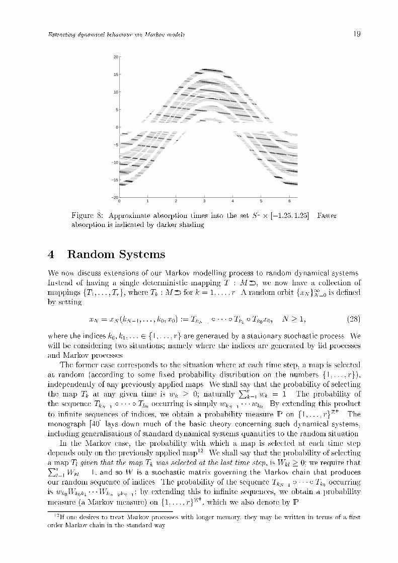
where � � �� represents the phase of the table at impact� v � R the velocity of the balljust after impact with the table� and T represents the evolution from one impact to the nextsee �� for details� We set � �� and � � �� for the remainder of this example� Figure �shows a typical orbit of the system� and Figure � shows an approximation of the �physical�invariant measure � again� there is good agreement between the two distributions� Wesuppose that we are interested in the time between successive impacts where the velocity ofthe ball is very low that is� we create a time series by counting the time intervals betweeninstances when the ball leaves the table with a velocity of magnitude less than �� ThusB � S� � �� in the earlier notation� Performing the analysis described above�Table � shows the results for various partition re�nements�

Compare these values with �� and �� the mean and variance re�spectively obtained directly from �� orbits of length �� plus!minus one standard deviationof the �� values obtained��

The result of the calculation of �n is shown in Figure �� It is clear that there is a sharpdivide between areas which return to low velocities relatively quickly �the very dark stripsin Figure �� and those areas that take longer to return� A histogram plot of � reveals thatif a point does not return very quickly to B� then it takes a much longer time�

�� Froyland

0 1 2 3 4 5 6−20

−15

−10

−5

0

5

10

15

20

Figure �� Plot of orbit of length �� for the bouncing ball map�

0 1 2 3 4 5 6−20

−15

−10

−5

0

5

10

15

20

Figure �� Approximate invariant measure for the bouncing ball map using �� partition sets� Darker regions indicate higher density�

Table �� Estimates of the mean and variance of return times to the set B � S� ��

Number of partition sets n �� Mean Mn �� Root Variance

pVn ��


0 1 2 3 4 5 6−20

−15

−10

−5

0

5

10

15

20

Figure �� Approximate absorption times into the set S� � �� Fasterabsorption is indicated by darker shading�

� Random Systems

We now discuss extensions of our Markov modelling process to random dynamical systems�Instead of having a single deterministic mapping T � M �

�

�� we now have a collection ofmappings fT�� Trg� where Tk � M �

�

� for k � �� r� A random orbit fxNg�N�� is de�nedby setting

xN � xN �kN�� k�� x�� TkN�� Tk� � Tk�x�� N � ��

where the indices k�� k�� f�� rg are generated by a stationary stochastic process� Wewill be considering two situations namely where the indices are generated by iid processesand Markov processes�

The former case corresponds to the situation where at each time step� a map is selectedat random �according to some �xed probability distribution on the numbers f�� rg��independently of any previously applied maps� We shall say that the probability of selectingthe map Tk at any given time is wk � � naturally

Prk��wk � �� The probability of

the sequence TkN�� Tk� occurring is simply wkN��

� � �wk� � By extending this product

to in�nite sequences of indices� we obtain a probability measure P on f�� rgZ�� The

monograph �� lays down much of the basic theory concerning such dynamical systems�including generalisations of standard dynamical systems quantities to the random situation�

In the Markov case� the probability with which a map is selected at each time stepdepends only on the previously applied map�� We shall say that the probability of selectinga map Tl given that the map Tk was selected at the last time step� is Wkl � � we require thatPr

l��Wkl � �� and so W is a stochastic matrix governing the Markov chain that producesour random sequence of indices� The probability of the sequence TkN��

� � � � � Tk� occurringis wk�Wk�k� � � �WkN��kN��

by extending this to in�nite sequences� we obtain a probability

measure �a Markov measure� on f�� rgZ�� which we also denote by P�

��If one desires to treat Markov processes with longer memory� they may be written in terms of a �rstorder Markov chain in the standard way�

�� Froyland

Examples ��

�i� Consider the bouncing ball map of the last section� Suppose that our ball is non�uniform� and that one side is more �springy� than the other� Sometimes� the ball willland on the springy side� and sometimes it will land on the not�so�springy side� Whichside the ball lands on determines the value of � and so at each time step there is arandom choice of � and therefore an application of either Tspringy or Tnot�so�springy

� Wereturn to this example later�

�ii� A set of maps fT�� Trg could arise as perturbations of a single map T viaTkx �� Tx � k� where k � Rd is a perturbation� We choose a probability vector�w�� wr� where the value wk represents the probability of our map T encounteringthe perturbation k� A random iid composition of the fTkg models a deterministicsystem subjected to small iid perturbations�

�iii� Random dynamical systems can also arise in the context of dynamical systems withinputs� The eect of an input is essentially to produce dierent dynamics �in otherwords� a dierent map Tk� at the time step in which it occurs� If the model is trulyrandom� these inputs could occur according to an iid process or Markov process� How�ever� more structured sets of inputs can also be modelled by Markov processes� forexample� where a randomly selected input triggers a �xed sequence of inputs beforeanother random input is selected�

We now de�ne what is meant by an invariant measure for our random system�

De�nition �� Let " � f�� rgZ�� and for � � �� "� de�ne the left shift

� � " �

�

� by ��i � �i�� The probability measure P on " introduced earlier is ��invariant�De�ne the skew product � � "�M �

�

� by �� x� � �� T�x� our random orbits fxNgN�may be written as xN � ProjM��N �� x�� where ProjM denotes the canonical projectiononto M �

We will say that a probability measure � on M is an invariant measure for our randomsystem� if there exists a � �invariant probability measure �� on "�M such that

�i� ��E �M� � P�E� for all measurable E � "� and

�ii� ��"� B� � ��B� for all measurable B �M �

De�nition �� A probability measure � is called a natural or physical measure for arandom dynamical system if � is de�ned as ��B� � ��" � B� where �� is a � �invariantprobability measure satisfying

limN��

�

N

N��Xk��

f��k�� x��Z�M

f�� x� d�� x� ��

for all continuous f � "�M R� and P�m almost all �� x� � "�M �

Remark �� If we choose the continuous test function f in �� to be independent of ��then we have the simple consequence that�

limN��

�

N

N��Xj��

f�Tkj � � � � � Tk�x�ZM

f d� � ��

for Lebesgue almost all x �M and P almost all random sequences of maps�


By setting f�x� � �A�x�� where A �M is such that ��A� � �� then

�

Ncardf� � j � N � � Tkj � � � �Tk� � Tk�x � Ag ��A��

again for Lebesgue almost all x �M and P almost all random sequences�

In rough terms� this says that if you plot the points in a random orbit de�ned by �� thenfor Lebesgue almost all starting points x� and P almost all random sequences of maps� oneobtains the same distribution of points� From the point of view of analysing the averagebehaviour of the random system� this is the correct distribution to approximate� The physicalmeasure � is usually not invariant under any of the individual transformations Tk� in thesense that � � T��k �� However� � is �invariant on average�� which by heavily abusingnotation may be written as E��T��k � � �� In the iid case� this formula is entirely accurate�as there the invariance condition is simply

Prk��wk� � T��k � ��

�� Basic constructions

We must construct a transition matrix

Pn�k� �m�An�i � T��k An�j�

m�An�i��

for each of the maps Tk�

Remark �� An alternative de�nition of the matrix Pn�k� is as follows� Within each setAn�i select a single point an�i� Then set

P �n�k� �

�� if Tkan�i � An�j�

�� otherwise��

Clearly� the computational eort involved in the numerical construction of P �n�k� is less than

that of Pn�k� in � �� especially in higher dimensions �in the Tips and Tricks section� wediscuss other numerical methods of computing Pn�k�� We do not recommend using P �

n�k�for deterministic systems� as the results are usually very poor� However� for random systems�one can still obtain quite good results with the cruder approximation of � ��

How these matrices are combined depends on whether the stochastic process is iid orMarkov�

iid case In the iid case� we set

Pn �rX

k��

wkPn�k� � �

Markov case In the Markov case� let W be the transition matrix for the Markov processthat generates the random sequence of indices for the maps fTkg�

Now set

Sn �

�BBBB�W�� Pn�� W�� Pn�� W�r Pn��

W�� Pn�� W�� Pn�� W�r Pn��

��

��

Wr� Pn�r� Wr� Pn�r� � � � Wrr Pn�r�

�CCCCA � � ��

�� Froyland

In both the iid and Markov cases� the matrices Pn and Sn may be thought of as �nite�dimensional projections of an �averaged� Perron�Frobenius operator see �� for details�With either of these two matrices� one may apply the methods described in x to estimateinvariant objects such as invariant measures� invariant sets� Lyapunov exponents� and recur�rence times�

�� Invariant measures

iid case We calculate the �xed left eigenvector pn of Pn as constructed in � �� and nor�malise so that

nXi��

pn�i � ��

Set �n�An�i� � pn�i and de�ne the approximate invariant measure as in ��

Markov case We calculate the �xed left eigenvector of Sn� and denote this as sn ��s

��n js��n j � � � js�r�n � where each s

�k�n � k � �� r is a vector of length n� and

Prk��

Pni�� s

�k�n�i � ��

De�ne the approximate invariant measure as

�n�An�i� �rX

k��

s�k�n�i � ��

We now use �� again to de�ne a measure on all of M �Results parallel to those of Theorem �� hold for our random systems�

Proposition �� Suppose that each Tk � M �

�

� is continuous and the resulting randomdynamical system has a physical measure � �in the weaker sense where only �� need hold�rather than �� Let f�ng denote a sequence of approximate invariant measures as de�nedin either � � or �� above� and let �� be a weak limit of this sequence� Denote by S theintersection

T�n�n�

supp�n� Then the conclusions of Theorem �� hold�

Proof� One �rst requires the facts that the matrices � � and � �� represent a �nite�dimensional approximation of an appropriately averaged Perron�Frobenius operator thisis detailed in �� With this established� the proofs run along the same lines as thedeterministic case� �

Example �� The �non�uniform bouncing ball� We now suppose that our bounc�ing ball has gone soft on one side� so that sometimes we register a value of � �� ratherthan the original value of � �� We assume that every time it lands on the soft side� itwill surely land on the good side next time� while if it lands on the good side� it has a ��!��chance of landing on the soft side next time� The situation we describe is a Markov randomcomposition of two mappings T�� and T�� The transition matrix for this Markov chain

is W �

��

� �

�� where � �� is identi�ed with state �� and � �� with state ��

We construct Sn as in � �� and compute the approximate invariant measure as in � �� seeFigure �� Again� there is good agreement between the two �gures�

��The form of �� is slightly di�erent to the matrix given in �� as we have performed a similaritytransformation on the latter to yield a more intuitive representation�


0 1 2 3 4 5 6−20

−15

−10

−5

0

5

10

15

20

Figure �� Plot of orbit of length �� for the random bouncing ball map

0 1 2 3 4 5 6−20

−15

−10

−5

0

5

10

15

20

Figure �� Approximate invariant measure for the random bouncing ball map using�� partition sets


In certain situations� one is able to obtain rigorous upper bounds for the dierence between�n and ��

The �rst of these is where the random system contracts phase space on average� Typicalexamples of such systems are the iterated function systems �IFS�s� of Barnsley � � and co�workers� where a �nite number of mappings are selected using an iid law to create fractalimages� Suppose that Tk is selected with probability wk� and de�ne sk � maxx�y�M kTkx Tkyk�kx yk as the Lipschitz constant for Tk then set s �

Prk��wksk� It is straightforward

to show that if s � �� then this random dynamical system has a unique invariant measure�

�� Froyland

the support of which is a fractal set� Furthermore� one has the bound�� see also ��

dH�� n� � � � s

� smax��i�n

diam�An�i��

where dH is the natural metric generating the weak topology on measures� de�ned bydH�� sup

��RMh d��

RMh d��

�� h � M R has Lipschitz constant �� If a uni�

form grid is used� this bound may be improved by a factor of �� Similar results hold forMarkov compositions� Ulam�type methods of approximating invariant measures of IFS�s arealso discussed in the book ��

The second situation is where the dynamical system is expanding on average� This settingis more complicated as the random system may have in�nitely many invariant measures�and it is important to show that Ulam�s method approximates the physical measure �inthis expanding case� the physical measure will have a bounded density�� In the case of iidrandom dynamical systems on the interval �� where each map Tk is a Lasota�Yorke map�it is known that a bounded invariant density exists provided that

Prk��wk�jT �k�x�j � �

see �� Under some additional conditions� it is shown in �� that �i� the random system�either iid or Markov� possesses a unique bounded invariant density� and �ii� that the Ulamestimates �n converge to the physical measure � �which has a bounded density�� In addition�convergence rates of O�logn�n� for the dierence k� �nkL� are proven� and if each Tk isa C� map of the circle S�� rather than of the interval �� explicitly calculable numericalbounds for the error k� �nkL� are given� In the future� we will no doubt see extensions ofthese results to higher dimensions�

�� Lyapunov exponents

The random version of �� is

�� limN��

�

Nlog kDxN��

TkN�� Dx�Tk� �DxTk��v�k� � ��

Often� the same value of is obtained for P almost all random sequences� Lebesgue almostall x �M � and for every v � Rd� We denote this value by ��

Things are very simple in the case of one�dimensional systems driven by an iid process�In this case� the expression � �� may be alternately expressed as

�rX

k��

wk

ZM

log jT �k�x�j d��x� � ��

by a straightforward application of �� with f�� x� � log jT ��x�j� Thus� once we have anestimate of the physical measure �� it is easy to compute an approximation of via

n ��rX

k��

wk

ZM

log jT �k�x�j d�n�x� �rX

k��

wk

nXi��

log jT �k�xn�i�j � pn�i� ��

where xn�i � An�i �for example� the midpoint of the interval An�i��

��This rigorous result holds even when the crude approximation of Remark �� is used�



For random systems� we adopt Approach �� of x � � as the other two approaches are not sohelpful in the random situation� Here we only brie#y describe the calculation of Lyapunovexponents of iid random dynamical systems where the Jacobian matrices are constant� Thissituation arises when each of the mappings Tk are a�ne �as with most IFS�s�� Equation� �� now becomes independent of the x�� xN�� and is a function only of the sequencek�� kN�� we are essentially dealing with an iid random matrix product�

Suppose that M is two�dimensional so that our Jacobian matrices are � � � matrices�We need to de�ne a probability measure � on the angle space RP� �� is a relativeof the probability measure alluded to in x � �� Each matrix DTk �note independence ofx� de�nes a map from �� to itself via angle�v� � angle�DTk�v�� where angle�v� is theangle between v and some �xed reference vector in R�� To simply notation� we will identifya vector v � R� and its angle with respect to some �xed reference vector� The Jacobianmatrix DTk will then be thought of as an action on the space of angles ��

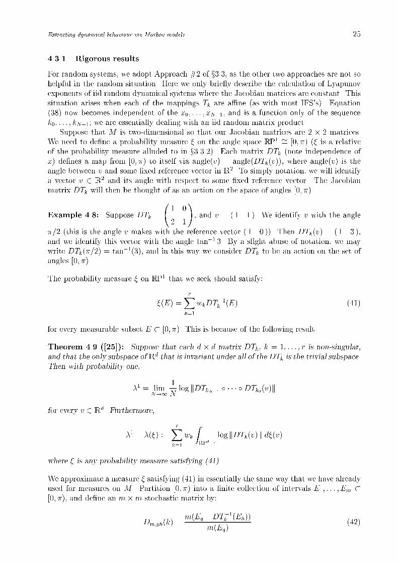
Example �� Suppose DTk �

��

� �

�� and v � � � � �� We identify v with the angle

�� this is the angle v makes with the reference vector � � � �� Then DTk�v� � � � ��and we identify this vector with the angle tan�� By a slight abuse of notation� we maywrite DTk�� tan�� and in this way we consider DTk to be an action on the set ofangles ��

The probability measure � on RP� that we seek should satisfy�

��E� �rX

k��

wkDT��k �E� ��

for every measurable subset E � �� This is because of the following result�

Theorem �� Suppose that each d � d matrix DTk� k � �� r is non�singular�and that the only subspace ofRd that is invariant under all of the DTk is the trivial subspace�Then with probability one�

� � limN��

�

Nlog kDTkN��

� � � � �DTk��v�k

for every v � Rd� Furthermore�

� � �� rX

k��

wk

ZRPd��

log kDTk�v�k d��v�

where � is any probability measure satisfying ��

We approximate a measure � satisfying �� in essentially the same way that we have alreadyused for measures on M � Partition �� into a �nite collection of intervals E�� Em �� and de�ne an m�m stochastic matrix by�

Dm�gh�k� �m�Eg �DT��k �Eh��

m�Eg��

�� Froyland

Alternatively �ala Remark �� one could choose a collection of points e�� em such thateg � Eg and set

Dm�gh�k� �

�� if DTk�eg� � Eh

�� otherwise��

or use the other suggestions in x�� One now computes the �xed left eigenvector of thematrix Dm �

Prk��wkDm�k� we denote this eigenvector by �m� Selecting points e�� em

as before� we de�ne an approximation of � as

�m ��rX

k��

wk

mXg��

log kDm�k��eg�k ��

where� in the expression kDm�k��eg�k� eg is a unit vector in the direction represented byeg� and we measure the length of the vector Dm�k��eg� �this is the factor by which Dm�k�stretches vectors in the direction of eg�� The above constructions may be generalised tohigher dimensions see �� for details� We have summarised the simplest situation here thetreatment of Markov random matrix products� and iid random nonlinear dynamical systemsmay be found in ��


To estimate the mean and variance of return times� we again construct a �nite Markovmodel� and calculate the mean and variance of return times to a suitable set of states� In theiid case we can de�ne a Markov model using � �� and proceed as for deterministic systems�

In the Markov case� we use � �� and produce a left eigenvector sn of Sn such thatPrk��

Pni�� s

�k�n�i � �� When writing Sn in the block form �� recall that each partition set

An�i corresponds to r states of the Markov chain governed by Sn� With this in mind� onemay substitute Sn and sn into the algorithm described in x �� It is also possible to considersituations where the set B depends on the map Tk which is currently applied ��

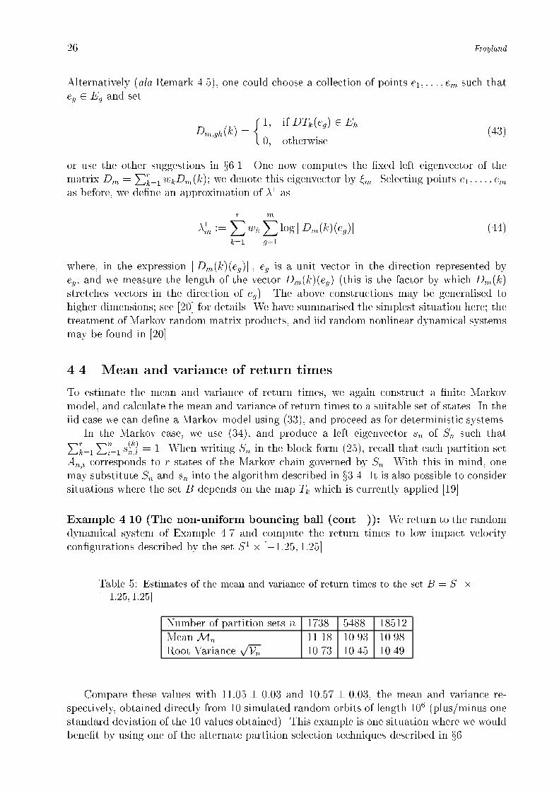
Example �� The non�uniform bouncing ball �cont�� We return to the randomdynamical system of Example �� and compute the return times to low impact velocitycon�gurations described by the set S� � ��

Table �� Estimates of the mean and variance of return times to the set B � S� ��

Number of partition sets n �� Mean Mn �� Root Variance

pVn ��

Compare these values with �� and �� the mean and variance re�spectively� obtained directly from �� simulated random orbits of length �� plus!minus onestandard deviation of the �� values obtained�� This example is one situation where we wouldbene�t by using one of the alternate partition selection techniques described in x��


�� Advantages for Markov modelling of random dynamical sys�

tems

To close this section� we discuss two further advantages of Markov modelling over trajectorysimulation that are not present in the deterministic case�

The �rst of these concerns the accuracy of the approximations� For deterministic systems�the two competing approaches �simulating long orbits and coarse graining� both have theirinaccuracies� The iterative approach of following long orbits �let�s assume that we can doperfect computations� has the problem of temporal deviation from equilibrium behaviour�That is� we should really have orbits of in�nite length� but instead we have orbits of �nitelength whose statistical behaviour is not the same� In contrast� with the Markov modellingapproach� we can exactly compute the long term behaviour of our model� but we compute thelong term behaviour of an approximation of the system� rather than that of the true system�Turning now to random systems� the iterative approach is �ghting errors on two frontsnamely� the deviation from equilibrium in phase space mentioned above� and additionally�the deviation of the distribution of the �nite length random sequence of indices k�� kN��from its equilibrium distribution P� On the other hand� the Markov modelling approachcompletely eliminates errors from the random #uctuations by averaging them out through theexpectations performed in its construction� Thus our Markov models for random dynamicalsystems do not suer from the inaccuracies due to random #uctuations� and are therefore�heuristically at least� more accurate this is borne out numerically in Lyapunov exponentcomputations ��

The second advantage lies in the #exibility of the Markov modelling approach regardingthe underlying stochastic process� Suppose that we wish to study a family of systems whichuse the same maps T�� Tr� but a dierent distribution P �in the bouncing ball example�this would amount to varying the probabilities with which impacts occur on the soft andhard sides�� Most of the computational eort goes into constructing the ��xed� transitionmatrices Pn�k�� k � �� r� while the ancillary calculations involving eigenvectors and soon� are relatively cheap� Thus� we may perform analyses on a whole family of systems veryquickly� by reusing most of the original constructions� In contrast� if we were to use the directmethod of simulating long orbits� then entirely new orbit calculations would be required foreach new set of probabilities�

� Miscellany

We brie#y outline some other applications and techniques related to our approach of Markovmodelling� Unless otherwise stated� we refer only to deterministic systems�

Global attractors Related partition�based methods may be used to approximate theglobal attractor for a given subset of phase space� If B � M � then the global attractorof B is de�ned by G �

Tk� T

j�B�� Methods of computing an �in principle�� rigorousbox covering of the global attractor are detailed in �� Bounds for the Hausdor distancebetween the approximate covering and the global attractor are given for uniformly hyperbolicdieomorphisms�

Using similar techniques� box coverings for global attractors G�� of individual samplepaths � of random dynamical systems have been studied � ��

��when combined with Lipschitz estimates for the map ��

�� Froyland

Work is in progress on covering �averaged� global attractors of random systems suchglobal attractors contain all possible random orbits and so Gav �

SG��

Noisy systems A popular idea is to �noise up� a system by considering the transformationx � Tx � � where the perturbation � R

d is chosen in a uniform distribution fromsome small ball centred around �� This may be viewed as de�ning a random dynamicalsystem where the collection of maps T� � Tx � are applied in an iid fashion with equalprobability� The Perron�Frobenius operator P� � L

��M�m� �

�

� for this random perturbationhas the desirable property that it is a compact operator under very mild conditions on T �and this greatly simpli�es the ergodic theoretic analysis� For example� it is relatively easyto show that this noisy system has a unique invariant probability density� in contrast to thepurely deterministic case� The �nite�state Markov modelling may now be applied to theperturbed system� and various convergence results proven concerning the approximation ofinvariant measures and invariant sets see �� This setting forms the basis of the thesis � ��where the merits of alternative partitioning methods are also considered�

Rotation numbers The approximation of rotation numbers of orientation preserving C�

circle dieomorphisms using Ulam constructions is described in ��

Topological entropy It is possible to obtain rigorous upper bounds for the topologicalentropy of T with respect to a �xed �coarse� partition� All orbits of T are possible under theMarkov model� however the converse is not true� In this sense� the Markov model is more�complex� from the orbit generating viewpoint� However� as the partitions are re�ned andour Markov model becomes more accurate� these extra orbits are successively eliminated� sothat our upper bounds become increasingly sharp� This is work in progress ��

Spectra of �averaged� transfer operators for random systems One may also at�tempt to garner dynamical information from the spectrum and eigenvectors of the matrices� � and � �� in analogy to the deterministic case� This is work in progress�

� Numerical Tips and Tricks

We discuss methods of computing the transition matrix and of partition selection� Most tran�sition matrix computations in this chapter have used the GAIO software package� availableon request from http��www�math�uni�paderborn�de��agdellnitz�gaio�� Algorithms�ii� and �iii� of x�� and �i� �iv� of x�� have been coded in this software�

�� Transition matrix construction

Techniques for the computation of the transition matrix may be split into three main classesnamely �exact� methods� Monte�Carlo!Imaging methods� and an exhaustive method of ap�proximation�

�i� �Exact� methods� For one�dimensional systems� it is often possible to construct thetransition matrix exactly� If the map is locally one�to�one on each partition set� thenonly the inverse images of the endpoints of each set need be calculated�


If the inverse images are di�cult to obtain� an alternative is to compute the matrix

P �n�ij �

m�TAi � Aj�

m�TAi��

which in one�dimension again requires only the computation of forward images ofpartition endpoints�

The matrix P �n is not useful theoretically because �i� forward images of sets may not be

measurable� while inverse images �T continuous� of Borel measurable sets are alwaysmeasurable� and �ii� the standard form � � arises as a discretisation of the Perron�Frobenius operator for T � while �� does not� If T is linear on each Ai� then Pij � P �

ij

for j � �� n this forward�imaging exact computation was carried out for two�dimensional piecewise linear reconstructions in �� Otherwise� the dierence betweenP and P � is governed by the second derivative of T and the diameter of the partitionsets� We do not recommend using forward�imaging for maps with very large secondderivatives�

�ii� Monte�Carlo � Imaging of test points� The most popular method is the so�calledMonte�Carlo approach � �� To compute Pij� one randomly selects a large number ofpoints fa�� aNg � Ai� and sets Pij � �fa � fa�� aNg � T �a� � Ajg�N � Asimilar approach is to choose a uniform grid of test points within each partition set�and perform the same calculation� My personal feeling is that the latter approachis better as the uniform grid more reliably approximates Lebesgue measure� Anynumber of variations on the selection of test points can be used� though Monte�Carloand uniform grids are the most common�

�iii� Exhaustion� A recent approach �� is to rigorously approximate the transition prob�ability by a means of exhaustion akin to the exhaustion methods of Eudoxus� Tocompute the Lebesgue measure of the portion of Ai that is mapped into Aj� one re�peatedly re�nes the set Ai until it is known �via Lipschitz estimates on the map� thata re�ned subset of Ai is mapped entirely inside Aj� In this way� the set Ai is re�peated broken down into small pieces which map entirely inside Aj� with this processterminating at the desired level of precision�

�� Partition selection

This section is devoted to suggesting methods of producing better Markov models via smarterpartition selection� That is� how should one choose partitions to best capture the dynamicsof the system�

Of course� if a Markov partition is available� this is clearly the best choice� However�we are assuming that this is not the case� and we are left with the decision of how toconstruct a suitable �grid�� For the most part� we consider partition selection where thecriteria for a good partition is that it produces a good estimate of the physical measure�at least a better estimate than a uniform grid would produce�� Of course� often we don�tknow what the physical measure is� and so this mostly restricts rigorous numerical testingto one�dimensional systems� Nevertheless� we outline three main approaches� and suggestheuristically when they may be useful� In all cases� one selects an initial coarse partition�computes the invariant measure for the Markov model� and on the basis of informationcontained in the invariant measure of the current model� a choice is made on which partitionsets to re�ne and which to not re�ne�

� Froyland

�i� Standard approach� Re�ne any partition sets which are currently assigned non�zeromeasure�

�ii� Equal mass approach� Re�ne any partition sets which are assigned a measure greaterthan ��n� where n is the current number of partition sets ��

The rationale behind this is that one should focus more �nely on regions where thereis large mass� In this sense� the method is not only targeted at obtaining more ac�curate estimates of the invariant measure� but also more accurate modelling of thedynamics of the system this has been demonstrated for the estimation of return timesin �� This method is particularly suited to systems which possess a singular phys�ical measure� as in dissipative chaotic systems� However� because of the non�uniformre�nement �the minimal ratio of cell sizes is almost always at least � if re�nementis done by �halving� a set�� it often performs worse than the standard method incases where the physical measure is smooth� For this approach to be useful� the ratiosupx�supp�n �n�x�� infx�supp�n �n�x� should be much larger than � for all n � � ��n isthe density of the approximate measure �n��

�iii� High derivative approach� Let ci denote the �centre point� of a partition set Ai� Re�nepartition sets where the value of

Ei �� m�Ai� diam�Ai�max

jpi�m�Ai� pj�m�Aj�jjci cjj � Aj is a neighbour of Ai

��

is greater than ��n�Pn

i��Ei � ��

The expression that is maximised over is meant to be an approximation of the derivativeof the invariant density � on Ai in the �direction of� Aj� In � �� one assumes that thephysical measure is smooth therefore� if the current estimate of the invariant measurehas adjacent sets given very dierent measures� there must be an error in this region�and so one re�nes these sets to obtain better estimates� The number Ei is intended toapproximate the error incurred on the partition set Ai�

An alternative viewpoint is as follows� In �� it is noted that the matrix �Pij ��Ai � T��Aj��Ai� is an optimal approximation in the sense that the �xed lefteigenvector �p of �P assigns exactly the correct weights to the partition sets that is��pi � ��Ai� �this approach is also followed in � �� The dierence between P and �Pis essentially given by how �non�Lebesgue�like� the measure � is within each partition

set roughly speaking� how �non constant� the distribution of � is within partition sets�One may try to reduce�� the error k� �nk� by creating a partition which producesa transition matrix P similar to that of the special matrix �P � Such an analysis alsoleads to the error minimisation criteria ��

The high derivative method is targeted speci�cally towards more accurate estimates ofthe physical measure� It often performs better than the equal mass approach for mapswith smooth densities�

�iv� Large di�erence approach � �� One re�nes all partition sets and constructs a temporarytransition matrix Ptemp and invariant measure ptemp for the re�ned partition� Thisre�ned invariant measure is compared with the invariant measure pold and only sets inthe old partition for which the measure according to ptemp and pold is very dierent are

��Such a �distortion reducing� approach is also discussed in �� for one�dimensional maps �in particular�the logistic family Tax � ax�� x�� and a relative of the Equal mass approach is advocated as a means tomake P better approximate �P �


split up� The transition matrix Ptemp is now discarded� This approach is based on astandard method of numerical analysis�

Comparisons of the three alternative approaches are detailed in � ��

� Acknowledgements

We thank Oliver Junge for helpful discussions and critical comments during the preparationof this chapter� and Oliver Junge and Stefan Sertl for assistance with the use of the GAIOpackage� The list of references is not meant meant to be exhaustive� and is far from beingso� GF apologises for any oversights�

References

�� Ludwig Arnold� Random Dynamical Systems� Springer monographs in mathematics� Springer� Berlin��

�� Philip J� Aston and Michael Dellnitz� The computation of Lyapunov exponents via spatial integrationwith application to blowout bifurcations� Computer methods in applied mechanics and engineering��

�� Michael F� Barnsley� Fractals everywhere� Academic Press� Boston� ��

�� George D� Birkho�� Proof of the ergodic theorem� Proceedings of the National Academy of Sciences of

the USA� ��

�� J� R� Blum and J� I� Rosenblatt� On the moments of recurrence time� Journal of Mathematical Sciences��

�� Abraham Boyarsky and Pawel G�ora� Laws of Chaos � Invariant Measures and Dynamical systems in

One Dimension� Probability and Its Applications� Birkh auser� Boston� ��

�� Michael Dellnitz� Gary Froyland� and Stefan Sertl� On the isolated spectrum of the Perron�Frobeniusoperator� Submitted to Nonlinearity� ��

�� Michael Dellnitz and Andreas Hohmann� A subdivision algorithm for the computation of unstablemanifolds and global attractors� Numerische Mathematik� ��

�� Michael Dellnitz and Oliver Junge� Almost invariant sets in Chua�s circuit� International Journal of

Bifurcation and Chaos� ��

�� Michael Dellnitz and Oliver Junge� An adaptive subdivision technique for the approximation of attrac�tors and invariant measures� Computing and Visualization in Science� ��

�� Michael Dellnitz and Oliver Junge� On the approximation of complicated dynamical behavior� SIAMJournal on Numerical Analysis� ��

�� Jiu Ding and Aihui Zhou� Finite approximations of Frobenius�Perron operators� a solution of Ulam�sconjecture to multi�dimensional transformations� Physica D� ��

�� H� Francke� D� Plachky� and W� Thomsen� A �nitely additive version of Poincar�e�s recurrence theorem�In N� Christopeit� K� Helmes� and M� Kohlmann� editors� Stochastic Di�erential Systems � Proceedings

of the �rd Bad Honnef Conference� June �� Lecture Notes in Control and Information Science�Berlin� �� Springer�Verlag�

�� Gary Froyland� Finite approximation of Sinai�Bowen�Ruelle measures of Anosov systems in two dimen�sions� Random � Computational Dynamics� ��

�� Gary Froyland� Computer�assisted bounds for the rate of decay of correlations� Communications in

Mathematical Physics� ��

�� Gary Froyland� Approximating physical invariant measures of mixing dynamical systems in higherdimensions� Nonlinear Analysis� Theory� Methods� � Applications� ��

�� Gary Froyland� Ulam�s method for random interval maps� Nonlinearity� ��

� Froyland

�� Gary Froyland� Using Ulam�s method to calculate entropy and other dynamical invariants� Nonlinearity��

�� Gary Froyland and Kazuyuki Aihara� Estimating the mean and variance of interspike intervals� Inpreparation�

�� Gary Froyland and Kazuyuki Aihara� Rigorous numerical estimation of Lyapunov exponents and in�variant measures of iterated function systems and random matrix products� Int J Bifur Chaos� �� To appear�

�� Gary Froyland� Kevin Judd� and Alistair I� Mees� Estimation of Lyapunov exponents of dynamicalsystems using a spatial average� Physical Review E� ��

�� Gary Froyland� Kevin Judd� Alistair I� Mees� and Kenji Murao� Lyapunov exponents and triangulations�In Proceedings of the �� International Symposium on Nonlinear Theory and its Applications� Hawaii�

December �� volume �� pages ��

�� Gary Froyland� Kevin Judd� Alistair I� Mees� Kenji Murao� and David Watson� Constructing invariantmeasures from data� International Journal of Bifurcation and Chaos� ��

�� Gary Froyland� Oliver Junge� and Gunter Ochs� Rigorous computation of topological entropy of mul�tidimensional dynamical systems with respect to a �nite partition� In preparation�

�� Harry Furstenberg and Yuri Kifer� Random matrix products and measures on projective spaces� IsraelJournal of Mathematics� ��

�� Pawel G�ora� On small stochastic perturbations of mappings of the unit interval� Colloquium Mathe�

maticum� ��

�� Pawel Gora and Abraham Boyarsky� Absolutely continuous invariant measures for piecewise expandingC� transformations in RN � Israel Journal of Mathematics� ��

�� John Guckenheimer and Philip Holmes� Nonlinear Oscillations� Dynamical Systems� and Bifurcations

of Vector Fields� volume �� of Applied Mathematical Sciences� Springer�Verlag� New York� ��

�� R� Guder� M� Dellnitz� and E� Kreuzer� An adaptive method for the approximation of the generalizedcell mapping� Chaos� Solitons� and Fractals� ��

�� Rabbijah Guder and Edwin Kreuzer� Adaptive re�nement of the generalized cell mapping� Preprint��

�� Fern Y� Hunt� A Monte Carlo approach to the approximation of invariant measures� Random �

Computational Dynamics� ��

�� Oliver Junge� Mengenorientierte Methoden zur numerischen Analyse dynamischer Systeme� PhD thesis�University of Paderborn� Paderborn� ��

�� Oliver Junge� Rigorous discretization of subdivision techniques� In Proceedings of Equadi�� Berlin�

August � � ��

�� M� Kac� On the notion of recurrence in discrete stochastic processes� Bulletin of the American Mathe�

matical Society� ��

�� Michael Keane� Rua Murray� and Lai�Sang Young� Computing invariant measures for expanding circlemaps� Nonlinearity� ��

�� Gerhard Keller� Stochastic stability in some chaotic dynamical systems� Monatshefte f�ur Mathematik��

�� Gerhard Keller and Carlangelo Liverani� Stability of the spectrum for transfer operators� Preprint��

�� Hannes Keller and Gunter Ochs� Numerical approximation of random attractors� Institut f ur Dynamis�che Systeme� Universit at Bremen� Report Nr� �� August ��

�� R�Z� Khas�minskii� Principle of averaging for parabolic and elliptic di�erential equations and for Markovprocesses with small di�usion� Theory of Probability and its Applications� ��

�� Yuri Kifer� Ergodic Theory of Random Transformations� volume � of Progress in Probability and

Statistics� Birkh auser� Boston� ��


�� Yuri Kifer� Random Perturbations of Dynamical Systems� volume �� of Progress in Probability and

Statistics� Birkh auser� Boston� ��

�� Andrzej Lasota and Michael C� Mackey� Chaos� Fractals� and Noise Stochastic Aspects of Dynamics�volume � of Applied Mathematical Sciences� Springer�Verlag� New York� second edition� ��

�� Andrzej Lasota and James A� Yorke� On the existence of invariant measures for piecewise monotonictransformations� Transactions of the American Mathematical Society� ��

�� Tien�Yien Li� Finite approximation for the Frobenius�Perron operator� A solution to Ulam�s conjecture�Journal of Approximation Theory� ��

�� Walter M� Miller� Stability and approximation of invariant measures for a class of nonexpandingtransformations� Nonlinear Analysis� ��

�� Walter M� Miller and Fern Y� Hunt� Approximation of attractors for �nite dimensional maps by Ulam�smethod� Preprint� May ��

�� Rua Murray� Adaptive approximation of invariant measures� Preprint� ��

�� Rua Murray� Existence� mixing and approximation of invariant densities for expanding maps on Rd�Preprint� ��

�� Rua Murray� Approximation error for invariant density calculations� Discrete and Continuous Dynam�

ical Systems� ��

�� S� Pelikan� Invariant densities for random maps of the interval� Transactions of the American Mathe�

matical Society� ��

�� Mario Peruggia� Discrete Iterated Function Systems� A K Peters� Wellesley� ��

�� Karl Petersen� Ergodic Theory� volume � of Cambridge Studies in Advanced Mathematics� CambridgeUniversity Press� Cambridge� ��

�� David Ruelle� Ergodic theory of di�erentiable dynamical systems� IHES Publicationes Mathematiques��

�� Leonard A� Smith� The maintenance of uncertainty� In G� Cini Castagnoli and A� Provenzale� editors�Past and Present Variability of the Solar�Terrestrial system� Measurement� Data Analysis and Theo�

retical Models� volume CXXXIII of Proceedings of the International School of Physics� pages ��Amsterdam� �� Italian Physical Society�

�� Jaroslav Stark� Iterated function systems as neural networks� Neural Networks� ��

�� S� M� Ulam� Problems in Modern Mathematics� Interscience� ��

�� Bodo Werner and N� Nicolaisen� Discretization of circle maps� Zeitscrift f�ur Angewandte Mathematik

und Physik� ��

�� J� Wolfowitz� The moments of recurrence time� Proceedings of the American Mathematical Society��

�� Lai�Sang Young� Recurrence times and rates of mixing� To appear in Israel Journal of Mathematics�

gary froyland, in alistair mees, editor, nonlinear dynamics and

Documents