finite element procedures for time-dependent convection-diffusion-reaction systems · ·...

INTERNATIONAL JOURNAL FOR NUMERICAL METHODS IN FLUIDS, VOL. 7, 1013-1033 (1987)

FINITE ELEMENT PROCEDURES FOR TIME-DEPENDENT CONVECTION-DIFFUSION-REACTION SYSTEMS

T. E. TEZDUYAR*, Y. J. PARK? AND H. A. DEANS1

University of Houston, Houston, TX 77004, U.S.A.

SUMMARY

New finite element procedures based on the streamline-upwind/Petrov-Galerkin formulations are developed for time-dependent convection-diffusion-reaction equations. These procedures minimize spurious oscillations for convection-dominated and reaction-dominated problems. The results obtained for representative numerical examples are accurate with minimal oscillations.

As a special application problem, the single-well chemical tracer test (a procedure for measuring oil remaining in a depleted field) is simulated numerically. The results show the importance of temperature effects on the interpreted value of residual oil saturation from such tests.

KEY WORDS Convection-Diffusion-Reaction Finite Elements Petrov-Galerkin

INTRODUCTION

Many engineering problems are governed by convection-diffusion type equations with source terms. Fluid dynamics problems in the presence of body forces, chemically reactive flows and electrochemical interaction flows are only a few examples. In most of these cases the source (or sink) terms cause coupling in the set of governing differential equations. In this paper we focus on chemically reactive flows, with particular emphasis on time-dependent problems. Such problems involve temperature and concentrations as dependent variables. Prediction of these unknown variables is very important for the economical operation of various chemical engineering systems, including chemical reactors and enhanced oil recovery processes.

Chemically reacting systems are governed by a set of convection-diffusion-reaction equations derived from energy and material balance laws. The reaction terms are assumed to be expressions which are products of some function of the concentrations of the chemical components and an exponential function of the temperature. Therefore, unless the process is isothermal or the heat of reaction is negligible, the source terms result in a non-linear coupling in the equation set. If the heat of reaction is assumed to be small, the equation governing the temperature can be solved first independent of the concentrations. However, the concentration equations will still depend on the temperature field. Deans and Lapidus'.' and several other author^^-^ have investigated the chemical reactor problems by models and numerical analyses based on a uniform

Based on a contributed paper. *Assistant Professor, Department of Mechanical Engineering. f Graduate Research Assistant, Department of Chemical Engineering, on leave from Pusan Open National University, Korea. 1 Professor, Department of Chemical Engineering.

0271-209 1/87/101013-21!$10.50 0 1987 by John Wiley & Sons, Ltd.

1014 T. E. TEZDUYAR, Y. J. PARK A N D H. A. DEANS

velocity profile assumption. In practical applications the flow velocity may vary from one point to another substantially. Because of this the governing equations may vary in nature from convection-dominated to reaction-dominated.

Convection-dominated and reaction-dominated cases pose a significant challenge for numerical solution of convection-diffusion-reaction type equations. It is well known that the regular (Bubnov-) Galerkin finite element formulations (or the classical centred finite difference schemes) result in spurious oscillations for convection-dominated problems, especially in the presence of sharp fronts in the solution. For reaction-dominated problems, in the presence of sharp gradients in the solution due to high reaction rates, one may again encounter numerical oscillations. This may occur if the flow velocity at a point approaches zero.

Several Petrov-Galerkin formulations have been proposed for convection-dominated problems. Among them are streamline-upwind/Petrov-Galerkin (SUPG) formulation^,^-^ 'sigma weighting' and 'transport weighting' schemes," and the 'discontinuity capturing term' approach.' l S 1 These methods have successfully been applied to various problems governed by the convection-diffusion, Navier-Stokes and compressible Euler equations. In Reference 12 a numerical diffusion/Petrov-Galerkin method was developed for steady-state reaction-dominated problems.

In this paper we develop a SUPG-based finite element formulation for time-dependent convection-diffusion-reaction equations. For reaction-dominated problems we add second-order terms proportional to the element Damkoehler number to the differential equations. These second- order terms are determined based on a one-dimensional accuracy analysis for a two-component linear reaction system. We show that for such systems nodal exactness can be achieved. The contributions of the numerical second-order terms become significant only where the reaction rates are very high.

Numerical solution of convection-diffusion-reaction equations has a wide range of applications in the area of oil recovery. An important application is the simulation of the single-well chemical tracer (SWCT) m e t h ~ d . ' ~ . ' ~ The SWCT method was developed to measure the residual oil saturation after water flooding an oil reservoir. The method depends on chromatographic separation caused by the local equilibrium distribution of each tracer between flowing and non- flowing fluids. A major advantage of the SWCT is that the tracers are produced back into the same wellbore from which they are injected into the target formation. This avoids various complications which might occur if the tracers were transported to and produced from a nearby well. A secondary tracer, which is produced during the 'shut-in' period by chemical reaction, makes it possible to avoid reversing the separation of the tracers when the flow is reversed during production.

In past simulations material balance equations for the tracers were solved assuming constant temperature in the formation. This does not account for the fact that the temperature of the injection fluid is almost always lower than the reservoir temperature. In our simulations we obtain more reliable residual oil saturation values by considering the effect of the temperature of the injection fluid on the reservoir temperature distribution. This is important because both the reaction rates and the equilibrium distributions of tracers depend on the temperature field. For this problem we compare our numerical results to field data.

In section 2 the problem statement is given. The finite element formulation and the analysis of the reaction-dominated flows are described in Sections 3 and 4. Numerical examples are presented in Section 5. The SWCT application is covered in Section 6. Conclusions are given in Section 7.

2. PROBLEM STATEMENT

Let R be an open region of WSd, where I Z , ~ is the number of space dimensions, and let r and

TIME DEPENDENT CONVECTION-DIFFUSION-REACTION SYSTEMS 1015

SZ denote its boundary and closure respectively. Spatial and temporal co-ordinates are denoted by XESZ and t € [ O , TI.

Consider the following system of ndof partial differential equations, with ndof being the number of degrees of freedom:

(1) pi a$'/& + u.V$' - V*(K~.V$') + R' = 0, i = 1,2,. . . , n d o f ,

where $'(x, t ) is the ith dependent (unknown) variable. The velocity field is represented by u, and pi and K~ are the accumulation capacity and diffusion tensor for the ith variable. The source/sink term R' in our cases is due to chemical reaction; it is through this term that the equations are linearly or non-linearly coupled. We assume that the velocity field is given, and is divergence free, That is,

v . u = o . (2) The boundary r is assumed to be decomposed as follows:

r = r,,urh, , (3)

@=r,,nrh2. (4)

$'(x, t ) = &, t ) , VxEr,,, t ~ ( 0 , T ) , i = L2, . . . , n d o f , ( 5 )

n(X)'Ki(X)' v$i(x, t ) = hi(x, t) , vxerh,, tE(O, T ) 7 i = 1 9 2 9 . . . 7 ndof 9 (6)

The boundary is allowed to have both Dirichlet and Neumann conditions given, respectively, by

where n is the unit outward normal vector to the boundary and gi and hi are prescribed functions. The initial/boundary-value problem for (1) consists of finding the unknown vector variable { $ i }

on Sr which satisfies (l), the boundary conditions (5) , (6), and the following initial condition:

$'(x,O) = $b(x), i = 1,2,. . . ,rldof, (7) where $h is a given function.

For the application problems we study in this paper, the equations of (1) are derived from the appropriate material and energy balance laws. In all cases, we have two chemical components A and B with concentrations CA and CB as dependent variables. In some cases, depending on the chemical reaction model, we also have the temperature T as a dependent variable. Then the dependent variable vector ( I c l i ) is defined as follows:

For simplicity we consider only a first-order irreversible reaction

A - + b B , (9) where A is the reactant, B is the product, and b is the stoichiometric coefficient of the reaction. The source/sink (reaction) vector { R'} is given as

The chemical reaction term, expressed by the Arrhenius kinetics, is ko exp { - E/ (RT)} where ko

1016 T. E. TEZDUYAR, Y. J. PARK AND H. A. DEANS

is the reaction rate coefficient, E is the activation energy and R is the gas constant. The term pc, is the heat capacity per unit volume and AH the heat of reaction per mole of the reactant.

3. FINITE ELEMENT FORMULATION

Consider a discretization of R into element subdomains Re, e = 1,2,. . . n,,, where n,, is the number of elements. Let re denote the boundary of P. We assume

e'='1

The interior boundary is defined as n.1

rin,= (J re-r . e = 1

Let I/' and S' denote the finite-dimensional subsets of H'(R), defined as follows:

V i = { w i ( w i d P ( R ) , w'(x)=O, on xd-,,}, (14)

Si = { $ll $ ' d P ( R ) , $'(x) = gi , on Xd-, ,} . (15)

In this paper we assume that both subsets consist of the typical Co finite element interpolation functions.

The discrete variational form of (1) satisfying the boundary conditions (5) and (6) and the associated initial condition (7) is given as follows: find $ i ~ S i such that for all W'E V'

jfl { wip'$f, + wiu* V$' + V W ~ . ( K ~ . V$') + wiRi} dR

"I

Pi {pi$:, + u s V$i - V .(K'* V$') + R'} dR =

i = 1,2,. . . , ndof , (16)

Jflwi($i-$b)dR = 0 , i = 1,2 ,..., ndof,

where ( ),t denotes a time derivative and Pi is a perturbation to the weighting function w'. The Euler-Lagrange equations corresponding to ( 1 6) may be obtained by integration-by-parts:

n.1 r 2 J wi{pi+ft + u.V$' - V - ( K ~ - V ~ / + ) + R'} dC2 e = l ~e

where [ ] is the 'jump' operator. If the perturbation term P i is zero, (16) leads to a regular (Bubnov-) Galerkin formulation;


if Pi # 0 we obtain a Petrov-Galerkin formulation. The modified weighting function

(19) Gi = wi + pi

acts only in the element interiors and therefore can be discontinuous across element boundaries. Various formulations for P i within the framework of streamline-upwind/Petrov-Galerkin

(SUPG), sigma weighting and transport weighting have been proposed and successfully tested by Hughes and Brooks,6 Tezduyar and Hughes,' Hughes et ul." and Tezduyar and Ganj00.I~ The recent 'discontinuity-capturing term' approach of Hughes et ul." and Tezduyar and Park" add another component to wi which results in smooth but crisp representation of internal and boundary layers.

A consistent finite element discretization of (16) and (17) leads to a set of non-linear ordinary differential equations:

Md + N(d) = F , (20)

0) = do > (21) where d is the vector of (unknown) nodal values of { $i} , d is its time derivative, N is a non-linear vector function of d, F is the right-hand side constant vector and do is a given vector corresponding to the initial condition (7). These equations are solved by a predictor/multicorrector temporal integration scheme.16

We employ the following expression for the weighting function associated with the element node a, degree of freedom i:

iVi = N, + 5'(h/2)s.VNa. (22)

For isotropic diffusivity tensors K~ = K ~ I , where I is the identity tensor, the parameters of (22) are defined as follows:

. a'/3, Mi < 3, t'={1, a i > 3

(doubly asymptotic approximation; see Reference 7),

s = u/IIu II 9 (24)

h = 2(xls-VNaI)-' ('element length'),

ai = II u I1 h/(21ci) (element Peclet number).

a

4. REACTION-DOMINATED PROBLEMS

In a convection-reaction problem when the ratio of the reaction rate to the convection speed at a point tends to a large number, the problem locally becomes reaction dominated. Near the sharp gradients in the solution due to high reaction/convection ratios, numerical oscillations may appear. In this section we perform a one-dimensional accuracy analysis which is an extension of the one described by Tezduyar and Park." Consider the following linear convection-reaction equation with constant velocity u 2 0 and reaction rate B 2 0:

B$ + u*,s = 0 9 (27) where s is the distance measured in the direction of the velocity. Assuming a discretization along s with constant element length h, the exact solution at a mesh point j can be written as follows:


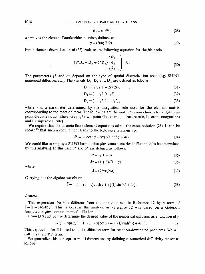
II/, = e - 2 ~ i J 9

where y is the element Damkoehler number, defined as

Finite element discretization

The parameters y* and 6*

7 = (m) of (27) leads to the following equation for the j th node:

depend on the type of spatial discretization used (e.g. SUPG, numerical diffusion, etc.). The stencils Do, D, and D, are defined as follows:

DO = (2r, 2( 1 - 2r), 2r),

D, = ( - 1/29 0,1/2) , D2 = ( - 1/2,1, - 1/2), (33)

where r is a parameter determined by the integration rule used for the element matrix corresponding to the reaction term. The following are the most common choices for r: 1/4 (one- point Gaussian quadrature rule), 1/6 (two-point Gaussian quadrature rule, i.e. exact integration) and 0 (trapezoidal rule).

We require that the discrete finite element equations admit the exact solution (28). It can be shown', that such a requirement leads to the following relationship:

6* = - cothy + y*(l/sinh2y + 4r). (34) We would like to employ a SUPG formulation plus some numerical diffusion i? (to be determined by this analysis). In this case y* and 6* are defined as follows:

Y*=Y/(l-Y),

6* = (1 + b))/(l - y) , where

b = (IZ/u)/(2/h).

Carrying out the algebra we obtain

b= -1-(1-y)cothy+y[(1/sin2y)+4r]. (38)

Remark

This expression .for b is different from the one obtained in Reference 12 by a term of [ - (1 - y)cothy]. This is because the analysis in Reference 12 was based on a Galerkin formulation plus some numerical diffusion.

From (37) and (38) we determine the desired value of the numerical diffusion as a function of y:

(39) This expression for i? is used to add a diffusion term for reaction-dominated problems. We will call this the DRD term.

We generalize this concept to multi-dimensions by defining a numerical diffusivity tensor as follows:

E(y) = u (h/2) { - 1 - ( 1 - y) coth y + y [ (1/ sinh2 y) + 4r] } .


where

and s and h are given by equations (24) and (25). The unit vectors t and v are orthogonal to s and to each other."

Extension to two-component systems

Consider the special case of (1) for a two-component linear reaction system:

I),: + U* V$' + B$' = 0,

$: + U' Vt,b2 - bB$' = 0 .

We propose to use an SUPG formulation on the following set of modified equations:

$,: + U* V$' + B$' = V.(P(y)- V$'),

$: + U' V$' - bB$' = - b V.(P(y)* V$' )

(42)

(43)

Whereas the modification of (42) is justified by the analysis presented above, the modification of (43) simply follows from (44). This is because both sets of equations (by multiplying the first equation by b and adding it to the second one) must give the same governing equation for (b$' + $2); that is

(46) (b$' + $2),t + u.V(b$' + $2) = 0.

5. NUMERICAL TESTS

Steady-state linear convection-reaction problem of a two-component system

In this problem we neglect the diffusion term in (1) and assume isothermal conditions. This case is very similar to the special case considered in section 4, given by equations (42) and (43). The problem involves two unknown concentration values CA and CB, i.e.

However, assuming that the boundary conditions co-operate, we need to solve only one equation for CA, since CB can be obtained from the following relationship:

bCA + CB = constant. (48)

u1 = u1(x2) = (1 - x$). (49)

Figure 1 (a) shows the 40 x 20 rectangular non-uniform finite element mesh used for this problem. The boundary conditions for component A are shown in Figure 1 (c). The parameters b and k, are selected to be 1.0 and 5.0. The exact solution has the form

The velocity is assumed to have a parabolic profile, descnbed as follows:

~ ~ = ~ ; e x p [ - k , x , / ( l -x:)], (50) where C; is the Dirichlet boundary condition at x1 =O. This problem becomes reaction

1020 T. E. TEZDUYAR, Y. J . PARK A N D H. A. DEANS

Figure 1 . Steady-state convection-reaction problem: (a) finite element mesh (40 x 20 element); (b) velocity profile; (c) boundary conditions

dominated when u1 approaches zero. The element Damkoehler number varies from 0.1 to infinity. Figure 2 shows the exact, SUPG and SUPG + DRD solutions for the concentration of component A. The SUPG solution exhibits a 57 per cent undershoot, whereas the SUPG + DRD scheme provides a significant improvement by resulting in no undershoot.

Time-dependent linear convection-reaction problem of a two-component system

This one-dimensional problem is governed by the time-dependent versions of the differential

TIME DEPENDENT CONVECTION-DIFFUSION-REACTION SYSTEMS

EXACT

Figure 2. Steady-state convection-reaction problem: elevation plots for the concentration of component A

1021


equations we had in the previous example. The flow parameters are selected to be pA = pB = 1.0, u = 1.0, b = 1.0 and k , = 1000. The spatial domain is [0,1] . The initial and boundary conditions are given as follows:

CA(x,O)=O, O < x < l , (51)

CB(x,O)=O, o < x < 1, (52)

[l - cos(27ct/t,)]/2, 0 < t < t , , 0, tat,,

C*(O, t ) = (53)

CB(0, t ) = 0, t > 0 , (54) where t , = 0.4.

In our finite element solution we use 50 elements. A Crank-Nicolson time integration scheme with a time step of 0.02 is employed. The flow parameters and the spatial and temporal discretizations lead to a Damkoehler number of 25 and a Courant number of 0.8. Note that for component A this problem is a highly reaction-dominated one. Figure 3 shows the exact, the SUPG and the SUPG + DRD solutions for components A and B. The SUPG solution exhibits undershoots up to 45 per cent for component A and overshoots up to 45 per cent for component B. The SUPG + DRD solution gives undershoots of less than 0.2 per cent for component A and no overshoots for component B. The SUPG ingredient of the algorithm minimizes the oscillations for the travelling wave solution of component B, whereas the DRD ingredient minimizes the oscillations due to high reaction rates.

6. APPLICATION: NUMERICAL SIMULATION OF THE SINGLE-WELL CHEMICAL TRACER METHOD

Background

A typical oil productive formation is a stratum of rock containing tiny interconnected pores which are saturated with oil, water and gas. Knowledge of the relative amounts of these fluids in the formation is indispensable to proper and efficient production of the formation hydrocarbons. For example, when a formation is first drilled it is necessary to know the original oil saturation to intelligently plan the future exploitation of the field. In tertiary recovery techniques, such as solvent flooding, the quantity of oil present in the formation after water flooding will often dictate the most efficient manner of conducting such an operation.

The single-well chemical tracer (SWCT) method was developed to measure the relative amount of fluid phases in a subterranean oil-bearing formation in which one of the phases is mobile and the others are essentially immobile. This method involves three time periods-injection, shut-in and production. During the injection period a carrier fluid containing a reactive tracer is injected into the oil-bearing formation through a well. After an appropriate amount of carrier-fluid-reactant solution has been injected, the solution is pushed farther away from the well by injection of reactant-free carrier fluid. The carrier-fluid-reactant solution is then permitted to remain at rest in the formation for a time. During this shut-in period a part of the reactant tracer reacts to form a product. Finally, the fluid is produced back into the same wellbore from which it was injected. Since the unconsumed reactant and the product have differing partition coefficients between the carrier fluid and the immobile phase, they are chromatographically separated in their passage through the formation during this production period. The amount of separation is a function of the saturation of the immobile fluid phase. The concentrations of reactant and


EXACT EXACT

0.2 0.4 0.6 0.8 1 . 0

D I STAN C,E

SUPG

0.8

0.6

V 0 . 4 -

0 .2 . .

-r "- : 0.2 0.4 0.6 0.e 7 . 0

DISTANCE

SUPG+DRD

0.2 0.4 0.6 0.8 1 . 0

DISTANCE

DISTANCE

SUPGcDRD

0.2 0 . 4 0.6 0.8 7. 0

DISTANCE DISTANCE

Figure 3. One-dimensional, time-dependent convection-reaction problem: concentration values for components A and B at time steps 16, 32,48 and 64. Element Courant number = 0.8, element Damkoehler number = 25


product are measured at the point of production and plotted versus produced volume. These results are matched by computer simulation of the equations governing the tracer behaviour during the three time periods. From the best fit, the relative proportions of mobile and immobile fluids in the formation can be determined.

An advantage of the SWCT method is that the sampled reservoir volume is much larger than that of other methods. This results in a more effective estimation of the residual oil saturation in the reservoir than would be possible by the other methods. The first field test was run in the East Texas Field in 1968, and the method was patented in 1971.13 Since then, about 160 SWCT tests have been performed wor1d~ ide . I~ In previous test simulations, material balance equations for tracers (one-dimensional time-dependent convection-diffusion-reaction equations) are normally solved to predict composition of the in situ fluid. Temperature has always been assumed to be constant.

The temperature of the injected fluid is normally lower than the reservoir temperature, causing a cooling effect near the well. This effect was not accounted for in previous numerical simulations. If the characteristic velocities of the temperature front and the reactive tracer are almost the same, the temperature shock may overlap the tracer bank during the reaction period. Since the chemical reaction rate is highly temperature dependent, the peak position of the product tracer may be displaced from that of the reactant tracer. Since the SWCT method depends on the separation of two tracers, deviation of the peaks in the formation affects the estimation of fluid saturation.

In order to account for the thermal effects on the SWCT method, heat transport by convection as well as conduction must be considered. This requires that the computational domain be at least a two-dimensional space containing the oil bearing permeable stratum as well as the underburden and overburden, which are the impermeable rock formations bounding the permeable stratum.

Governing equations

We assume that the problem is axisymmetric and select a cylindrical co-ordinate frame; i.e. (xl, x2) = ( r , z). The horizontal centre plane of the permeable stratum coincides with the plane z = 0. Appropriate to the SWCT configuration, the flow (which exists only in the permeable stratum) is radial and uniform in the z-direction. From the incompressibility condition of (2), the velocity field can be written as follows:

where U,, the radial Darcy velocity is given as

U r = q / ( 2 x r H ) .

Here q is the volumetric flow rate in the well, H is the height of the permeable stratum, 6 is the porosity of the stratum, and So, is its residual oil saturation. The governing equations for both the permeable and impermeable strata can be seen as special cases of equation ( 1 ) by appropriately defining the vectors and tensors involved.

We assume that the porous oil-bearing stratum is horizontal, homogeneous and incompressible, that the heat of reaction is negligible and that each unknown variable is always locally in equilibrium between phases. For the permeable stratum the vectors and tensors in (1) are defined as follows:


Components A and B are the reactant and product tracers. In the above equations, the subscripts o,r,w and f refer to oil, rock, water and fluid (oil and water) respectively. The distribution coefficients of the tracers between the oil and water phases K A and KB are determined experimentally as functions of temperature. The elements of the diagonal dispersion tensors are assumed to be linear functions of the components of the interstitial velocity vector v. That is

( D'k) = ( ::)vk, k = 1,. . . , nsd, D!k

where a is a scalar dispersion coefficient.

equation for the temperature can be obtained from ( 1 ) for ndof = 1 with For the impermeable stratum (rock) we have only one unknown, and that is the temperature. The

Boundary conditions and other parameters

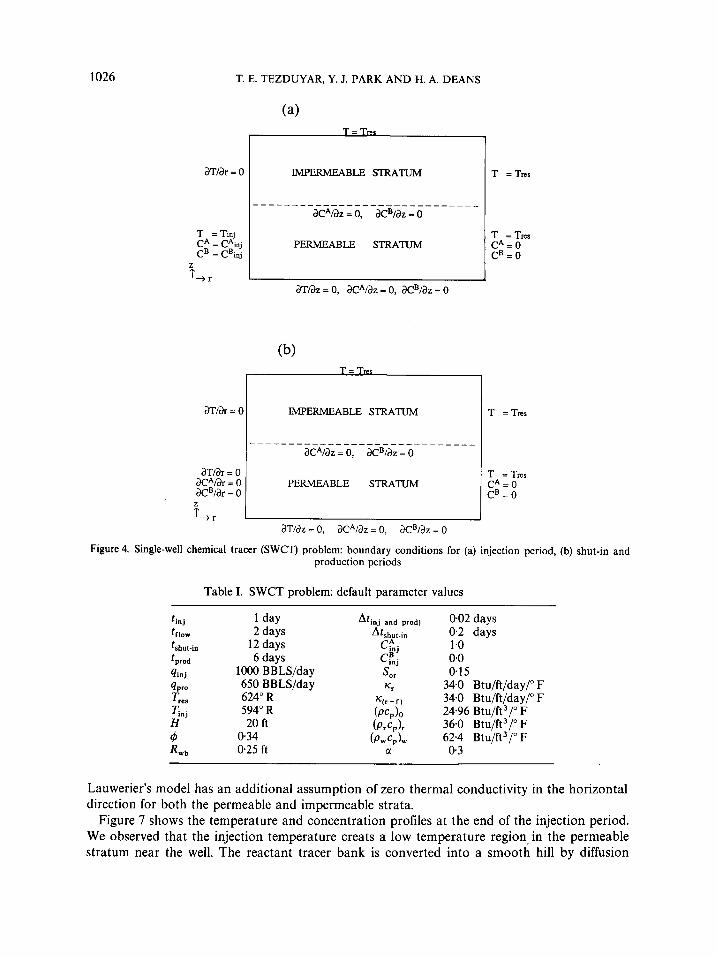
The computational domain is chosen such that the behaviour of the unknowns is known at the boundaries. For example, the horizontal centre plane of the porous stratum is taken as a boundary. Symmetry conditions along this plane provide no-flux conditions for all unknowns. The other boundaries are chosen far enough from the well in the horizontal direction and far from the interface of the permeable and impermeable strata in the vertical direction so that these boundaries are set to reservoir conditions. The boundary conditions for the three time periods are shown in Figure 4.

The default values of the parameters used in this simulation are given in Table I. Note that during the injection period Ckj becomes zero after t = 1 day.

Results

We have employed a 10 x 40 rectangular non-uniform finite element mesh (shown in Figure 5). The mesh is refined along the interface of the two strata because of the discontinuity of the velocity field along this line.

We have compared our numerical solutions (see Figure 6) for temperature to the analytical solutions of Lauwerier17 and Avdonin (in Spillette"). With respect to our model, Avdonin's model assumes infinite thermal conductivity in the vertical direction for the permeable stratum.

1026 T. E. TEZDUYAR, Y. J. PARK A N D H. A. DEANS

3nar = 0

T = Tinj CA = cA. . '"J cB = CBinj

z 1'+ r

IMPERMEABLE STRATUM T =Tns

PERMEABLE STRATUM T =Tres C A = O C B = 0

I 1 m a z = 0, a c A / a z = 0, a c B / a z = o

Figure 4. Single-well chemical tracer (SWCT) problem: boundary conditions for (a) injection period, (b) shut-in and production periods

Table I. SWCT problem: default parameter values

t inj 1 day tflow 2 days zshut-in 12 days tprod 6 days 4 i n j 1000 BBLS/day 4 p m 650 BBLS/day Tres 624" R 2 594" R

20 ft 4 0.34 RwLl 0.25 ft

0.02 days 0.2 days 1 .o 0 0 0.15

34.0 Btu/fi/day/" F 34.0 Btu/ft/day/" F 24.96 Btu/ft3/" F 360 Biu/fi3/o F 62.4 Btu/ft3/" F 0.3

Lauwerier's model has an additional assumption of zero thermal conductivity in the horizontal direction for both the permeable and impermeable strata.

Figure 7 shows the temperature and concentration profiles at the end of the injection period. We observed that the injection temperature creats a low temperature region. in the permeable stratum near the well. The reactant tracer bank is converted into a smooth hill by diffusion

TIME DEPENDENT CONVECTION-DIFFUSION-REACTION SYSTEMS I027

Figure 5. SWCT problem: finite element mesh (40 x 20 elements)

5 . 7 0 . 7 5 . 20. 2 5 .

DISTANCE r ( f t )

Figure 6. Comparisons with analytical solutions for the SWCT problem: the average temperature profile during the injection period, qinj = 200 BBLSlday

during the injection period. Concentration of the product tracer is almost zero because of the slow reaction rate.

Figure 8 shows the temperature and concentration profiles at the end of the shut-in period. Thermal diffusion results in the smoothing of the temperature profile. We observe a decrease for component A and an increase for component B, caused by reaction during the shut-in. At the end of the shut-in period the peak positions of the two tracers are 1 foot apart, as shown by the contour plots of Figure 9. This is caused by the temperature effect on reaction rate.

Figure 10 shows the temperature and concentration profiles after two days of production flow. The low temperature region in the porous stratum diminishes because of the backward convection of the reservoir temperature. Since the characteristic velocity of the product tracer is higher than that of the reactant tracer, most of the product tracer has been produced out, whereas a substantial part of the reactant tracer remains in the reservoir.

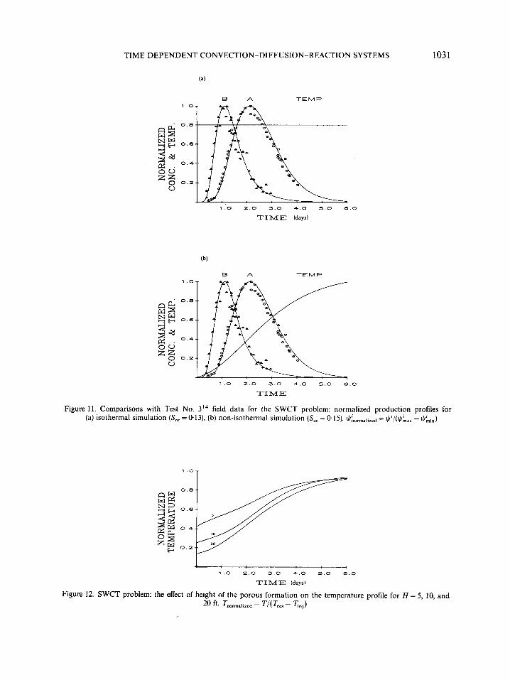
Production profiles for the isothermal and non-isothermal simulations are shown in Figure 11. By matching the numerical solution to specific field data (Reference 14, test no. 3) we estimate


Figure 7. SWCT problem: elevation plot (at the end of the injection period) for (a) temperature, (b) concentration of tracer A, (c) concentration of tracer B

TIME DEPENDENT CONVECTION-DIFFUSIONREACTION SYSTEMS 1029

Figure 8. SWCT problem: elevation plot (at the end of the shut-in period) for (a) temperature, (b) concentration of tracer A, (c) concentration of tracer B

0

0 (ft) 29

Figure 9. SWCT problem: contour plot (at the end of the shut-in period) for (a) concentration of tracer A, (b) concentration of tracer B

Figure 10. SWCT problem: elevation plot (at the end of the production period) for (a) temperature, (b) concentration of tracer A, (c) concentration of tracer B

TIME DEPENDENT CONVECTION-DIFFUSION-REACTION SYSTEMS

1 0

0 s

0.6

0.4

0.2

1 . 0 2.0 5.0 4.0 5.0 6.0

TIME (days)

1 .o

0.6

0.6

0 . 4

0.2

1031

1 . 0 2.0 3.0 4.0 5.0 6.0

T I M E

Figure 11. Comparisons with Test No. 314 field data for the SWCT problem: normalized production profiles for (a) isothermal simulation (SOr = 0.13). (b) non-isothermal simulation (Sor = 0.15). $&rmalired = $'/($Lax -$hi.)

1 1 .o

1 . 0 2.0 3.0 4 .0 5.0 6.0

TIME (days)

Figure 12. SWCT problem: the effect of height of the porous formation on the temperature profile for H = 5, 10, and 20 ft. Tnormalized = '/('re, - Tnj)

1032 T. E. TEZDUYAR. Y. J. PARK AND H. A. DEANS

an oil saturation value of 13 per cent for the isothermal case. The resulting residual oil saturation value is 15 per cent for the non-isothermal simulation. Since no temperature history data are available for the SWCT field test, we assumed that the injection temperature was 30" F lower than the reservoir temperature. The temperature differences, however, may be up to 150" F for high-temperature reservoirs. The higher the temperature difference, the higher the discrepancy will be between the estimated saturation value for the isothermal and non-isothermal simulations.

The thickness of the permeable formation may be estimated from the temperature histories if we know the thermal properties of the permeable and impermeable strata. Temperature production profiles for the same tracer test in three different porous formation thicknesses are depicted in Figure 12. As can be seen, the thicker the formation, the lower the early production temperature.

7. CONCLUSIONS

In this paper we have presented our new SUPG-based finite element procedures for time- dependent convection-diffusion-reaction equations. For reaction-dominated problems we have performed a one-dimensional accuracy analysis for a two-component linear reaction system. Based on this analysis we proposed a numerical diffusion/Petrov-Galerkin supplement for the SUPG formulations. This additional ingredient minimizes the spurious oscillations due to high reaction rates without introducing excessive numerical diffusion. The formulations were tested on steady-state and time-dependent reaction-dominated problems. The solutions obtained are accurate with minimal spurious oscillations.

As a special application, numerical simulation of the single-well chemical tracer test method was performed. With this simulation we have shown that temperature effects play an important role because they influence the produced tracer profiles significantly. We have demonstrated that the cooling caused by injection fluid results in the peak location of the product tracer being further away than that of the reactant tracer. This effect leads to erroneously low values of residual oil saturation for the usual isothermal estimation. We also have observed that the temperature profiles, because they depend on the height of the permeable formation, can give some information about that height.

ACKNOWLEDGEMENTS

This research was sponsored by NASA-Johnson Space Center under contract NAS-9- 17380, by NSF under grant MSM-8552479 and by the Laboratory for Enhanced Oil Recovery, University of Houston. We are grateful for the computing resources made available by the Aeroscience Branch of the NASA-Johnson Space Center. Y. J. Park was partially supported by Pusan Open National University, Korea.

REFERENCES

1. H. A. Deans and L. Lapidus,'A computational model for predicting and correlating the behavior of fixed-bed reactors:

2. H. A. Deans and L. Lapidus, 'A c I mputational model for predicting and correlating the behavior of fixed-bed reactors:

3. B. A. Finlayson, 'Packed bed reactor analysis by orthogonal collocation', Chem. Eng. Sci., 26, 1082-1091 (1971). 4. G. F. Fromont and K. B. Bischoff, Chemical Reactor Analysis and Design, Wiley, New York, 1979. 5. V. Pinjala, 'Wrong-way behavior in fixed-bed catalystic reactors: pseudo-Homogeneous dispersion model', Ph.D.

6. T. J. R. Hughes and A. Brooks, 'A theoretical framework for Petrov-Galerkin methods with discontinuous weighting

1. Derivation of model for nonreactive systems', A.1.Ch.E. Journal, 6, (4), 656-663 (1960).

11. Extension to chemically reactive systems', A.l.Ch.E. Journal, 6, (4), 663-668 (1960).

Thesis, Chemical Engineering Department, University of Houston, 1985.


functions: application to the streamline upwind procedure’, in R. H. Gallagher, D. N. Norrie, J. T. Oden and 0. C. Zienkiewicz, Finite Elements in Fluids, Vol . IV, Wiley, Chichester, 1982, pp. 46-65.

7. A. N. Brooks and T. J. R. Hughes, ‘Streamline upwind/Petrov-Galerkin formulations for convection dominated flows with particular emphasis on the incompressible Navier-Stokes equations’, Computer Methods in Applied Mechanics and Engineering, 32, 199-259 (1982).

8. T. E. Tezduyar and T. J. R. Hughes, ‘Finite element formulations for convection dominated flows with particular emphasis on the compressible Euler equations’, Proceedings of A I A A 21 st Aerospace Sciences Meeting, Reno, Nevada, January 1983, A I A A Paper 83-0125.

9. T. J. R. Hughes, M. Mallet and L. Franca, ‘New finite element methods for the compressible Euler equations’, R. Glowinski and J. L. Lions (eds), Computing Methods in Applied Sciences and Engineerings V I I , North-Holland, Amsterdam, pp. 339-360.

10. T. J. R. Hughes, M. Mallet, Y. Taki, T. Tezduyar and R. Zanutta, ‘A one-dimensional shock capturing finite element method and multi-dimensional generalizations’, in F. Angrand, A. Dervieux, J. A. Desideri and R. Glowinski (eds), Numerical Methods for the Euler Equations of Fluid Dynamics, SIAM 1985, pp. 371-408.

11. T. J. R. Hughes, M. Mallet, and A. Mizukami, ‘A new finite element formulation for computational fluid dynamics: 11. Beyond SUPG’, Computer Methods in Applied Mechanics and Engineering, 54, 341-355 (1986).

12. T. E. Tezduyar and Y. J. Park, ‘Discontinuity capturing finite element formulations for nonlinear convection- diffusion-reaction equations’, Computer Methods in Applied Mechanics and Engineering, 59, 307-323 (1986).

13. H. A. Deans, ‘Method for determining fluid-saturations in reservoir’, U.S. Patent N o . 3,623,842, November 1971. 14. H. A. Deans and S. Majoros, ‘The single-well chemical tracer method for measuring residual oil saturation, final report’,

DOE/BC/20006-18, October 1980. 15. T. E. Tezduyar and D. K. Ganjoo, ‘Petrov-Galerkin formulations with weighting functions dependent upon spatial

and temporal discretization: applications to transient convection-diffusion problems’, Computer Methods in Applied Mechanics and Engineering, 59, 49-71 (1986).

16. T. E. Tezduyar and T. J. R. Hughes, ‘Development to time-accurate finite element techniques for first-order hyperbolic systems with particular emphasis on the compressible Euler equations’, Report prepared under NASAIAmes Uniuersity Consortium Interchange N o . NCA2-OR745-I 04 .

17. H. A. Lauwerier, ‘The transport of heat in an oil layer caused by the injection of hot fluid’, Appl. Sci. Res. Section A , 5, 145-150 (1955).

18. A. G. Spillette, ‘Heat transfer during hot fluid injection into an oil reservoir’, The Journal of Canadian Petroleum Technology, 4, (4), 2 13-2 18 (1 965).

finite element procedures for time-dependent convection-diffusion-reaction systems · ·...

Documents