Takustraße 7D-14195 Berlin-Dahlem

GermanyKonrad-Zuse-Zentrumfur Informationstechnik Berlin

MARTIN WEISER

Pointwise Nonlinear Scaling forReaction-Diffusion-Equations

ZIB-Report 07-45 (December 2007)

Pointwise Nonlinear Scaling for

Reaction-Diffusion-Equations

Martin Weiser

December 28, 2007

Abstract

Parabolic reaction-diffusion systems may develop sharp moving reactionfronts which pose a challenge even for adaptive finite element methods. Wepropose a method to transform the equation into an equivalent form that usu-ally exhibits solutions which are easier to discretize, giving higher accuracy fora given number of degrees of freedom. The transformation is realized as anefficiently computable pointwise nonlinear scaling that is optimized for pro-totypical planar travelling wave solutions of the underlying reaction-diffusionequation. The gain in either performance or accuracy is demonstrated on dif-ferent numerical examples.AMS MSC 2000: 65M60, 65M50

Keywords: reaction-diffusion equations, travelling waves, nonlinear scaling,discretization error

1 Introduction

Reaction-diffusion equations are used to model a tremendous amount of effects, inparticular in chemistry, biology, and material sciences. They describe the spatio-temporal distribution of one ore more species subject to diffusion and nonlinear in-teraction. Due to their importance in practical applications, a considerable amountof effort has been spent on the numerical solution.

One of the outstanding properties of reaction-diffusion equations is the existenceof travelling waves, which are moving reaction fronts. An accurate representationof reaction fronts is usually necessary in computations to capture the front speedcorrectly. If the diffusion is small compared to the computational domain and thereaction speed, the reaction fronts can be rather sharp. A quantitatively faithfulresolution of sharp reaction fronts is quite challenging for numerical methods, sincea rather small mesh size is required. Uniform meshes are often inefficient or evenuseless due to the exceedingly large number of unknowns they incur. For this reason,

1

2

adaptive mesh refinement techniques are widely used, in particular for finite elementdiscretizations.

In Rothe’s method, standard h-, p-, and hp-refinement are used for the stationaryelliptic problems arising in each time step, along with mesh coarsening in regionsof the domain which the front has left behind. More specialized approaches such asanisotropic refinement [1,7] or different refinement levels for variables with differentsmoothness [12] are effective, but difficult to implement, in particular in combina-tion with maintaining a mesh hierarchy for geometric multigrid solvers. Domaintransformations and vertex relocations, so-called r-refinement, have been provento be efficient for one-dimensional problems [11] and have also been studied for 2Dand 3D problems with some success [2,8]. Drawbacks are the overhead of additionalPDEs describing the mesh movement and the difficult treatment of geometricallycomplex boundaries.

Unlike the linear wave equation that advances waves of arbitrary shape with thesame speed, reaction-diffusion equations often allow only a small number of waveshapes to be propagated at all, with the wave speed depending on the wave shape.Thus, the local solution structure is to some extent determined by the travellingwave solutions of the reaction-diffusion equation. In this paper, we try to exploit thisfact and propose an analytical preprocessing based on planar travelling waves. Thepreprocessing is a pointwise nonlinear scaling of the range that aims at smoothingout sharp reaction fronts. The approach requires analytical preprocessing and istherefore much less general than mesh refinement, but since only a pointwise scalingis involved, the implementation effort is negligible and the computational overheadrather small.

The remainder of the paper is organized as follows. In section 2, the concept ofpointwise nonlinear scaling is introduced formally. The main section 3 is devotedto the development of a framework for computing optimal scalings for spatial finiteelement discretizations. This is transferred to time discretizations in the followingsection 4. Finally, scaling for spatio-temporally adaptive methods is considered insection 5.

2 Pointwise Nonlinear Scaling

Let us consider a simple scalar reaction-diffusion equation of the form

u = div(κ∇u) + f(u) in Ωu = uD on ∂ΩD

∂nu = γ(uN − u) on ∂ΩN = ∂Ω\∂ΩD.

(1)

Here, Ω is a domain in Rd and f : R→ R is a smooth function.

3

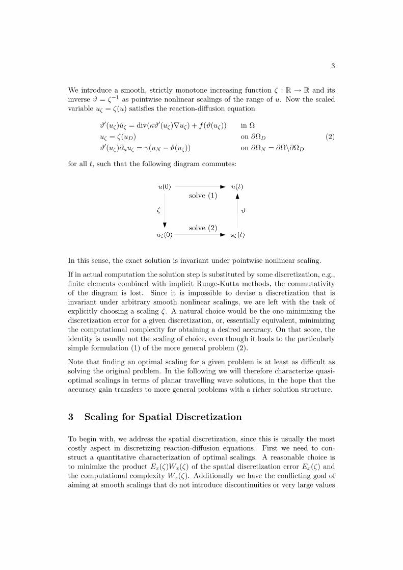
We introduce a smooth, strictly monotone increasing function ζ : R → R and itsinverse ϑ = ζ−1 as pointwise nonlinear scalings of the range of u. Now the scaledvariable uζ = ζ(u) satisfies the reaction-diffusion equation

ϑ′(uζ)uζ = div(κϑ′(uζ)∇uζ) + f(ϑ(uζ)) in Ωuζ = ζ(uD) on ∂ΩD

ϑ′(uζ)∂nuζ = γ(uN − ϑ(uζ)) on ∂ΩN = ∂Ω\∂ΩD

(2)

for all t, such that the following diagram commutes:

solve (1)

solve (2)

In this sense, the exact solution is invariant under pointwise nonlinear scaling.

If in actual computation the solution step is substituted by some discretization, e.g.,finite elements combined with implicit Runge-Kutta methods, the commutativityof the diagram is lost. Since it is impossible to devise a discretization that isinvariant under arbitrary smooth nonlinear scalings, we are left with the task ofexplicitly choosing a scaling ζ. A natural choice would be the one minimizing thediscretization error for a given discretization, or, essentially equivalent, minimizingthe computational complexity for obtaining a desired accuracy. On that score, theidentity is usually not the scaling of choice, even though it leads to the particularlysimple formulation (1) of the more general problem (2).

Note that finding an optimal scaling for a given problem is at least as difficult assolving the original problem. In the following we will therefore characterize quasi-optimal scalings in terms of planar travelling wave solutions, in the hope that theaccuracy gain transfers to more general problems with a richer solution structure.

3 Scaling for Spatial Discretization

To begin with, we address the spatial discretization, since this is usually the mostcostly aspect in discretizing reaction-diffusion equations. First we need to con-struct a quantitative characterization of optimal scalings. A reasonable choice isto minimize the product Ex(ζ)Wx(ζ) of the spatial discretization error Ex(ζ) andthe computational complexity Wx(ζ). Additionally we have the conflicting goal ofaiming at smooth scalings that do not introduce discontinuities or very large values

4

of higher derivatives of the scaled solution uζ . We thus define the desired scalingas a minimizer of

minζ

Ex(ζ)Wx(ζ) +α

2‖ζ(s)‖2L2(R) s.t. ζ ′ > 0, (3)

where s > 1 is chosen appropriately for the underlying discretization of uζ . Forfinite elements of order p, a value of s = p+ 1 seems reasonable.

Discretization error model. Using finite elements of order p on a triangulationT of the domain Ω for discretizing the scaled solution uζ as uhζ , we assume thefollowing local approximation error estimate holds on each element T ∈ T of themesh:

‖uζ − uhζ ‖L2(T ) ≤ chp+1T |uζ |Hp+1(T )

Here, c is some generic constant independent of the diameter hT of the element T .Defining the discretized unscaled solution as uh = ϑ(uhζ ), we obtain the followingasymptotic error estimates for the unscaled solution:

‖u− uh‖L2(T ) = ‖ϑ(uζ)− ϑ(uhζ )‖L2(T )

≤ ‖ϑ′(uζ)‖L∞(T )‖uζ − uhζ ‖L2(T )

≤ chp+1T ‖ϑ′(uζ)‖L∞(T )|uζ |Hp+1(T ) (4)

As a continuous model of (4) we introduce the local mesh size h : Ω → R+ anddefine the local L2 error density pointwise as

exζ(x) = h(x)p+1ϑ′(uζ(x))|u(p+1)ζ (x)|, (5)

such that we can bound the overall error by

‖u− uh‖L2(Ω) ≤ c‖exζ‖L2(Ω).

Consequently, we define our error quantity as

Ex(ζ) = ‖exζ‖2L2(Ω).

In passing we note that a slightly longer computation yields a related error model

exζ(x) = h(x)p+1(ϑ′(uζ(x)) + ϑ′′(uζ(x))|∇uζ(x)|

)|u(p+1)ζ (x)|

for the H1 error, such that ‖u − uh‖H1(Ω) ≤ ‖exζ‖L2(Ω). For notational simplicity,however, we will concentrate on the L2 estimates.

Complexity model. Using an efficient solver, the computational complexity forcomputing uhζ is proportional to the number of elements in the mesh. From themesh size distribution h we can approximate the number of elements as

Wx(ζ) =∫

Ωh(x)−d dx (6)

for isotropic elements.

5

Mesh models. Note that both Ex and Wx and hence the minimizer ζ of (3) dodepend on the mesh size distribution h. Here we restrict our attention to meshesresulting from the two commonly encountered mesh refinement strategies: uniformmeshes and adaptively refined meshes.

For uniformly refined meshes we may assume h to be constant, such that

Ex(ζ)Wx(ζ) = c ‖ϑ′(uζ)u(p+1)ζ ‖2L2(Ω). (7)

For adaptively refined meshes we assume equilibration of local errors (4), which inour continuous model means that exζ is constant. We then have

h(x) = c∣∣∣ϑ′(uζ(x))u(p+1)

ζ (x)∣∣∣−1/(p+1)

,

such thatEx(ζ)Wx(ζ) = c

∫Ω

∣∣∣ϑ′(uζ)u(p+1)ζ

∣∣∣d/(p+1)dx (8)

holds.

Solution model. Unfortunately, the unknown solution u enters into exζ . Thus weneed to find an easily computable substitute that exhibits the same local structureand features as the solution u.

We assume that in most of the domain Ω the solution looks locally like a planartravelling wave. This assumption neglects effects frequently encountered in reaction-diffusion patterns, such as curvature-dependent wave speed, anisotropic diffusion,a continuum of wave forms and speeds, and boundary effects. Nevertheless, theplanar travelling wave assumption should capture the bulk of the local solutionstructure mostly correct and is moreover analytically and numerically tractable dueto its inherent one-dimensional nature. Thus, we look for nonlinear scalings thatare optimal for planar travelling waves.

Let us assume that (1) has a sufficiently smooth planar travelling wave solutionu(x, t) = w(x1 + σt), w : R → [0, 1], such that w is essentially constant outside[a, b]. Now we can substitute w for u and [a, b] for Ω.

Practical restrictions. For the numerical computation of ζ to be practical, onemore aspect has to be considered. Since w(x) is assumed to be contained in [0, 1], wemay essentially restrict our attention to scalings mapping [0, 1] into itself. However,actual solutions may well exceed this range, such that ζ needs to be representedon whole R. Since the travelling wave substitute w does not provide any informa-tion outside [0, 1], we select the most simple representation: linear extension. Wetherefore restrict ζ to the admissible set

Z = ζ : R→ R|ζ(0) = 0, ζ(1) = 1, ζ ′ > 0, supp ζ(k) ⊂ [0, 1] for k = 2, . . . , s.

6

Combining all above considerations, we end up with the optimization problems

minζ∈Z

∫ b

a

∣∣∣ϑ′(wζ)w(p+1)ζ

∣∣∣r dx+α

2‖ζ(s)‖2L2([0,1]) (9)

to solve for optimal scalings ζ for uniformly (r = d/(p+ 1)) and adaptively (r = 2)refined meshes, respectively.

One particularly nice property of this approach to select optimal scalings is thatthe result is essentially independent of the diffusion coefficient κ determining thewidth of the reaction front.

Lemma 3.1. Let u(x, t) = w(x+σt) be a travelling wave solutions of (1) for κ = 1on Ω = R and ζ(α) = arg minξ Ex(ξ)Wx(ξ) + α

2 ‖ξ(s)‖2L2(Ω) the associated optimal

scaling. Then, for every 0 < κ ∈ R, ζκ(α) = ζ(κ1/2−r(p+1)/2α) is an optimal scalingassociated to the travelling wave solution uκ(x, t) = w(x/

√κ+σt) of (1) on Ω = R.

Proof. A short calculation shows that uκ(x, t) = w(x/√κ+σt) is indeed a travelling

wave solution of (1). Without loss of generality we assume t = 0. By the chainrule, we have

∂p+1x ζ(uκ(x)) = ∂p+1

x ζ(w(x/√κ)) = κ−(p+1)/2∂p+1

ξ ζ(w(ξ))

for ξ = x/√κ. By the substitution rule, we have

Eκx(ζ)W κx (ζ) =

∫R

∣∣∣ϑ′(uκζ(x))u(p+1)κζ (x)

∣∣∣r dx=∫

R

∣∣ζ ′(w(x/√κ))−1∂p+1

x ζ(w(x/√κ)∣∣r dx

=∫

R

∣∣∣ζ ′(w(ξ))−1κ−(p+1)/2∂p+1ξ ζ(w(ξ))

∣∣∣r√κ dξ= κ1/2−r(p+1)/2

∫R

∣∣∣ζ ′(w(ξ))−1∂p+1ξ ζ(w(ξ))

∣∣∣r dξ= κ1/2−r(p+1)/2E1

x(ζ)W 1x (ζ).

Choosing ακ = κ1/2−r(p+1)/2α results in a simple scaling of the objective in (9) thatdoes not change the minimizers.

3.1 Numerical Examples

In the previous section, we have characterized optimal scalings as minimizers of thework per accuracy ratio. The associated objective yields a prediction of the errorreduction for uniform meshes or the savings in computational work for adaptivemeshes. However, this prediction comes from an idealized model situation. The

7

error and work model are continuous and do not take the necessarily discrete struc-ture of the mesh into account. Moreover, the error model is just a worst-case modelwith limited predictive power for an actual situation.

The most important simplification is that, the characterization of ζ is based onplanar travelling waves. In 2D/3D problems, the solution structure can be muchricher due to source terms, boundary conditions, and complex geometries. It isnot clear a priori, to which amount the error reduction transfers to more complexsettings. The first numerical example given in Section 3.1.1 is therefore a simple1D interpolation problem suitable for testing the work and error models.

3.1.1 1D Travelling Wave Approximation

As a first illustration of the effect of pointwise nonlinear scaling on the discretizationerror we consider the piecewise linear interpolation of a reaction front. As anarbitrary front shape we select the tangens hyperbolicus on the interval Ω1 = [−5, 5]:

w(x) =12

(tanhx+ 1)

Equidistant Interpolation. First, we approximate ζ by solving (9) with r = 2numerically using Ipopt [13] on a simple equidistant finite difference discretization.Since here we only aim at approximating w, we choose a rather small regularizationparameter α = 10−12.

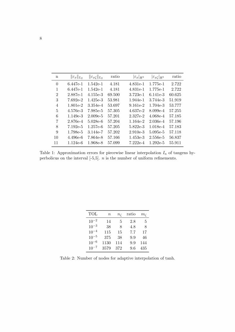
The obtained values for the estimated interpolation error are ‖ex‖L2(Ω) = 0.5164for the original and ‖exζ‖L2(Ω) = 0.0090 for the scaled problem, the ratio of whichgives an estimated error reduction factor of 57.2. The same ratio is obtained usingthe H1 norm for measuring errors. Then, both w and wζ are piecewisely linearlyinterpolated on an equidistant grid of 2n + 1 points, resulting in Inw and Inwζ ,respectively. The errors εnx = w − Inw and εxζ = w − ϑ(Inwζ) are evaluated ona further refined grid. The results given in Table 1 coincide very well with theprediction. The slight deterioration in the error reduction factor, which is visiblefor n = 11 in particular for the H1-error, can be attributed to the approximaterepresentation of ζ.

Adaptive Interpolation. As a second experiment, we solve (9) with r = d/(p+1), again choosing α = 10−12. The quotient of the obtained values for

∫h(x)−ddx

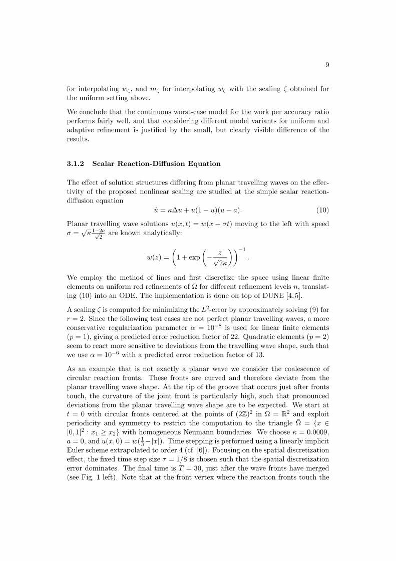
of 2.37 and 0.247 for the original and scaled problem, respectively, predicts a re-duction in the number of interpolation nodes by a factor of 9.6. Then w and wζare interpolated adaptively by bisecting the subinterval with the largest L2 errorcontribution until a given tolerance for the overall L2-error estimate is reached. Thenumber of interpolation nodes is reported in Table 2 as n for interpolating w, nζ

8

n ‖εx‖L2 ‖εxζ‖L2 ratio |εx|H1 |εxζ |H1 ratio

0 6.447e-1 1.542e-1 4.181 4.831e-1 1.775e-1 2.7221 6.447e-1 1.542e-1 4.181 4.831e-1 1.775e-1 2.7222 2.887e-1 4.155e-3 69.500 3.723e-1 6.141e-3 60.6253 7.692e-2 1.425e-3 53.981 1.944e-1 3.744e-3 51.9194 1.801e-2 3.354e-4 53.697 9.161e-2 1.704e-3 53.7775 4.576e-3 7.985e-5 57.305 4.637e-2 8.099e-4 57.2556 1.149e-3 2.009e-5 57.201 2.327e-2 4.068e-4 57.1857 2.876e-4 5.028e-6 57.204 1.164e-2 2.036e-4 57.1968 7.192e-5 1.257e-6 57.205 5.822e-3 1.018e-4 57.1839 1.798e-5 3.144e-7 57.202 2.910e-3 5.095e-5 57.118

10 4.496e-6 7.864e-8 57.166 1.453e-3 2.556e-5 56.83711 1.124e-6 1.968e-8 57.099 7.222e-4 1.292e-5 55.911

Table 1: Approximation errors for piecewise linear interpolation In of tangens hy-perbolicus on the interval [-5,5]. n is the number of uniform refinements.

TOL n nζ ratio mζ

10−2 14 5 2.8 510−3 38 8 4.8 810−4 115 15 7.7 1710−5 375 38 9.9 4610−6 1130 114 9.9 14410−7 3579 372 9.6 435

Table 2: Number of nodes for adaptive interpolation of tanh.

9

for interpolating wζ , and mζ for interpolating wζ with the scaling ζ obtained forthe uniform setting above.

We conclude that the continuous worst-case model for the work per accuracy ratioperforms fairly well, and that considering different model variants for uniform andadaptive refinement is justified by the small, but clearly visible difference of theresults.

3.1.2 Scalar Reaction-Diffusion Equation

The effect of solution structures differing from planar travelling waves on the effec-tivity of the proposed nonlinear scaling are studied at the simple scalar reaction-diffusion equation

u = κ∆u+ u(1− u)(u− a). (10)

Planar travelling wave solutions u(x, t) = w(x + σt) moving to the left with speedσ =√κ1−2a√

2are known analytically:

w(z) =(

1 + exp(− z√

2κ

))−1

.

We employ the method of lines and first discretize the space using linear finiteelements on uniform red refinements of Ω for different refinement levels n, translat-ing (10) into an ODE. The implementation is done on top of DUNE [4,5].

A scaling ζ is computed for minimizing the L2-error by approximately solving (9) forr = 2. Since the following test cases are not perfect planar travelling waves, a moreconservative regularization parameter α = 10−8 is used for linear finite elements(p = 1), giving a predicted error reduction factor of 22. Quadratic elements (p = 2)seem to react more sensitive to deviations from the travelling wave shape, such thatwe use α = 10−6 with a predicted error reduction factor of 13.

As an example that is not exactly a planar wave we consider the coalescence ofcircular reaction fronts. These fronts are curved and therefore deviate from theplanar travelling wave shape. At the tip of the groove that occurs just after frontstouch, the curvature of the joint front is particularly high, such that pronounceddeviations from the planar travelling wave shape are to be expected. We start att = 0 with circular fronts centered at the points of (2Z)2 in Ω = R2 and exploitperiodicity and symmetry to restrict the computation to the triangle Ω = x ∈[0, 1]2 : x1 ≥ x2 with homogeneous Neumann boundaries. We choose κ = 0.0009,a = 0, and u(x, 0) = w(1

3−|x|). Time stepping is performed using a linearly implicitEuler scheme extrapolated to order 4 (cf. [6]). Focusing on the spatial discretizationeffect, the fixed time step size τ = 1/8 is chosen such that the spatial discretizationerror dominates. The final time is T = 30, just after the wave fronts have merged(see Fig. 1 left). Note that at the front vertex where the reaction fronts touch the

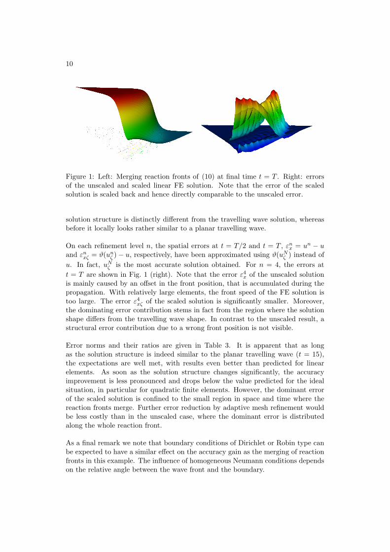
10

Figure 1: Left: Merging reaction fronts of (10) at final time t = T . Right: errorsof the unscaled and scaled linear FE solution. Note that the error of the scaledsolution is scaled back and hence directly comparable to the unscaled error.

solution structure is distinctly different from the travelling wave solution, whereasbefore it locally looks rather similar to a planar travelling wave.

On each refinement level n, the spatial errors at t = T/2 and t = T , εnx = un − uand εnxζ = ϑ(unζ )− u, respectively, have been approximated using ϑ(uNζ ) instead ofu. In fact, uNζ is the most accurate solution obtained. For n = 4, the errors att = T are shown in Fig. 1 (right). Note that the error ε4

x of the unscaled solutionis mainly caused by an offset in the front position, that is accumulated during thepropagation. With relatively large elements, the front speed of the FE solution istoo large. The error ε4

xζ of the scaled solution is significantly smaller. Moreover,the dominating error contribution stems in fact from the region where the solutionshape differs from the travelling wave shape. In contrast to the unscaled result, astructural error contribution due to a wrong front position is not visible.

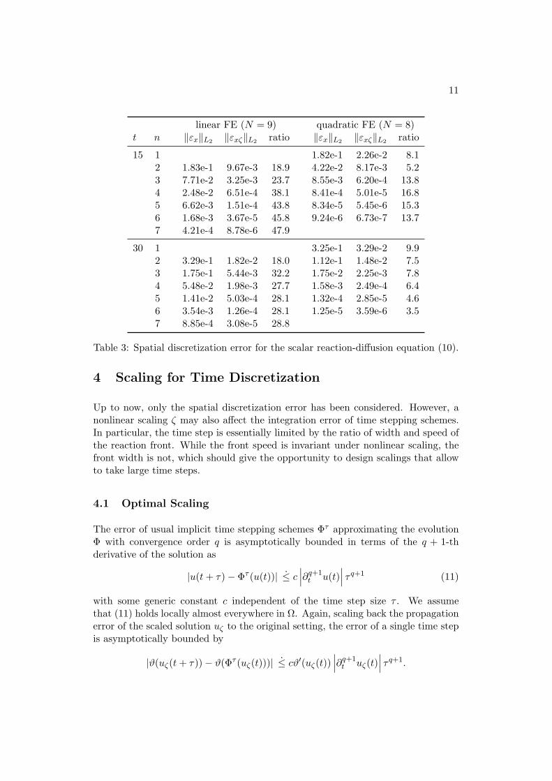
Error norms and their ratios are given in Table 3. It is apparent that as longas the solution structure is indeed similar to the planar travelling wave (t = 15),the expectations are well met, with results even better than predicted for linearelements. As soon as the solution structure changes significantly, the accuracyimprovement is less pronounced and drops below the value predicted for the idealsituation, in particular for quadratic finite elements. However, the dominant errorof the scaled solution is confined to the small region in space and time where thereaction fronts merge. Further error reduction by adaptive mesh refinement wouldbe less costly than in the unscaled case, where the dominant error is distributedalong the whole reaction front.

As a final remark we note that boundary conditions of Dirichlet or Robin type canbe expected to have a similar effect on the accuracy gain as the merging of reactionfronts in this example. The influence of homogeneous Neumann conditions dependson the relative angle between the wave front and the boundary.

11

linear FE (N = 9) quadratic FE (N = 8)t n ‖εx‖L2 ‖εxζ‖L2 ratio ‖εx‖L2 ‖εxζ‖L2 ratio

15 1 1.82e-1 2.26e-2 8.12 1.83e-1 9.67e-3 18.9 4.22e-2 8.17e-3 5.23 7.71e-2 3.25e-3 23.7 8.55e-3 6.20e-4 13.84 2.48e-2 6.51e-4 38.1 8.41e-4 5.01e-5 16.85 6.62e-3 1.51e-4 43.8 8.34e-5 5.45e-6 15.36 1.68e-3 3.67e-5 45.8 9.24e-6 6.73e-7 13.77 4.21e-4 8.78e-6 47.9

30 1 3.25e-1 3.29e-2 9.92 3.29e-1 1.82e-2 18.0 1.12e-1 1.48e-2 7.53 1.75e-1 5.44e-3 32.2 1.75e-2 2.25e-3 7.84 5.48e-2 1.98e-3 27.7 1.58e-3 2.49e-4 6.45 1.41e-2 5.03e-4 28.1 1.32e-4 2.85e-5 4.66 3.54e-3 1.26e-4 28.1 1.25e-5 3.59e-6 3.57 8.85e-4 3.08e-5 28.8

Table 3: Spatial discretization error for the scalar reaction-diffusion equation (10).

4 Scaling for Time Discretization

Up to now, only the spatial discretization error has been considered. However, anonlinear scaling ζ may also affect the integration error of time stepping schemes.In particular, the time step is essentially limited by the ratio of width and speed ofthe reaction front. While the front speed is invariant under nonlinear scaling, thefront width is not, which should give the opportunity to design scalings that allowto take large time steps.

4.1 Optimal Scaling

The error of usual implicit time stepping schemes Φτ approximating the evolutionΦ with convergence order q is asymptotically bounded in terms of the q + 1-thderivative of the solution as

|u(t+ τ)− Φτ (u(t))| ≤ c∣∣∣∂q+1t u(t)

∣∣∣ τ q+1 (11)

with some generic constant c independent of the time step size τ . We assumethat (11) holds locally almost everywhere in Ω. Again, scaling back the propagationerror of the scaled solution uζ to the original setting, the error of a single time stepis asymptotically bounded by

|ϑ(uζ(t+ τ))− ϑ(Φτ (uζ(t)))| ≤ cϑ′(uζ(t))∣∣∣∂q+1t uζ(t)

∣∣∣ τ q+1.

12

Note that errors need not be damped out in nonlinear parabolic equations. Inparticular, errors in the front position will be propagated forever. Thus we presumethe local integration errors sum up. Again substituting uζ by a travelling wave wζ ,we define the global propagation error density at time t

etζ = ϑ′(uζ(t))∂q+1t uζ(t)τ q = ϑ′(wζ)∂

q+1t wζ(·+ σt)τ q = ϑ′(wζ)σq+1w

(q+1)ζ τ q. (12)

Since uζ is a travelling wave, we may restrict our attention to t = 0 and constantstep sizes. The amount of work for a fixed time interval is then Wt = τ−1. Wetherefore have to minimize the quantity

τ q−1σq+1‖ϑ′(wζ)w(q+1)ζ ‖2L2(Ω1).

The time step enters only as a constant multiplicative factor and has no impact onthe minimizer if the regularization parameter α is scaled appropriately, such thatwe may discard τ and arrive at the minimization problem

minζ∈Z

∫ b

a

∣∣∣ϑ′(wζ)w(q+1)ζ

∣∣∣2 dx+α

2‖ζ(s)‖2L2([0,1])

Unsurprisingly, this is the same minimization problem as (9), derived for spatiallyuniform discretizations of corresponding order. The reason is that space x and timet are interchangeable in a travelling wave solution, up to the constant wave speedfactor.

4.2 Time Stepping

A difficulty introduced by the nonlinear scaling from (1) to (2) is the solution-dependent factor ϑ′(uζ) in front of the time derivative uζ . Simplifying notation, inthis paragraph we will consider ODEs of the form

B(u)u = f(u). (13)

In the extrapolated linearly implicit Euler method, now the solution of linear sys-tems with different matrices B(uk)− τA with A = f ′(u0) in every sub-timestep k isrequired. The computational complexity can be reduced by iterative solution usinga preconditioner or factorization of B(u0) − τA, see [6]. Still, the matrix B(uk)needs to be computed, and the implementation is more complex.

An attractive alternative is to rewrite (13) as a differential algebraic system

u = z

0 = f(u)−B(u)z, (14)

to which, e.g. Rosenbrock methods can be applied (cf. [10]). Due to the specialstructure of (14), the auxiliary variable z can be eliminated analytically, which

13

gives rise to a computationally cheap method. The same is possible for the linearlyimplicit Euler method, which then reads

(B(u0)− τA)δuk = τf(uk) + (B(u0)−B(uk))δuk−1 with δu−1 = 0.

The advantage is that the linear equation systems to be solved feature the samematrix and only different right hand sides, and that only the application of thedifference B(u0) − B(uk) to a vector needs to be computed. While this approachis computationally cheap and easy to implement, it has a significant drawback:Although the convergence order is retained, an increase in the error constant by afactor of 3 has been observed in the following examples. The reported results aretherefore based on the direct approach above.

A further important aspect is deliberate sparsing of the Jacobian. While the or-der of Rosenbrock methods in general relies on the exact value A = f ′(u0), theextrapolated linearly implicit Euler method is a W-method and as such its orderis independent of the approximation quality of A ≈ f ′(u0). Note that in generalW-methods are limited to second order [9], but can achieve higher orders for certainclasses of problems. With the freedom of choosing A arbitrarily, we can modify theJacobian in order to accelerate the linear solver on one hand, e.g. by droppingentries, or to reduce the error constant of the W-method on the other hand. Bothaspects depend on the actual problem, and the optimal choice can thus depend onthe chosen nonlinear transformation. Changes in the error constant by a factor of10 have been observed in the numerical examples below.

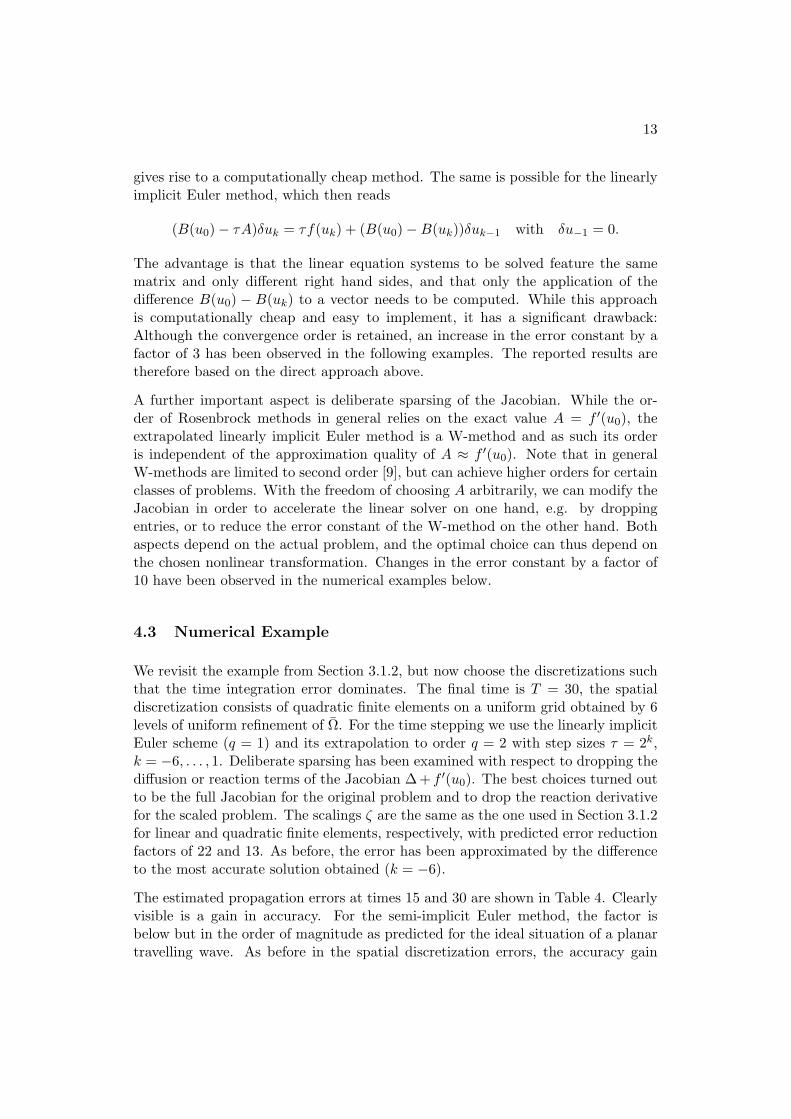
4.3 Numerical Example

We revisit the example from Section 3.1.2, but now choose the discretizations suchthat the time integration error dominates. The final time is T = 30, the spatialdiscretization consists of quadratic finite elements on a uniform grid obtained by 6levels of uniform refinement of Ω. For the time stepping we use the linearly implicitEuler scheme (q = 1) and its extrapolation to order q = 2 with step sizes τ = 2k,k = −6, . . . , 1. Deliberate sparsing has been examined with respect to dropping thediffusion or reaction terms of the Jacobian ∆ + f ′(u0). The best choices turned outto be the full Jacobian for the original problem and to drop the reaction derivativefor the scaled problem. The scalings ζ are the same as the one used in Section 3.1.2for linear and quadratic finite elements, respectively, with predicted error reductionfactors of 22 and 13. As before, the error has been approximated by the differenceto the most accurate solution obtained (k = −6).

The estimated propagation errors at times 15 and 30 are shown in Table 4. Clearlyvisible is a gain in accuracy. For the semi-implicit Euler method, the factor isbelow but in the order of magnitude as predicted for the ideal situation of a planartravelling wave. As before in the spatial discretization errors, the accuracy gain

14

Euler (q = 1) extrap. Euler (q = 2)t k ‖ε‖L2 ‖εζ‖L2 ratio ‖ε‖L2 ‖εζ‖L2 ratio

15 1 9.55e-2 3.32e-3 26.6 7.66e-3 1.79e-3 4.30 4.54e-2 2.32e-3 18.3 1.39e-3 4.85e-4 2.9

-1 2.10e-2 1.30e-3 15.8 2.88e-4 1.27e-4 2.3-2 9.77e-3 6.61e-4 14.8 6.67e-5 3.27e-5 2.0-3 4.47e-3 3.15e-4 15.0 1.62e-5 8.20e-6 2.0-4 1.89e-3 1.36e-4 17.1 3.84e-6 1.97e-6 2.0

30 1 2.41e-1 9.05e-3 28.8 2.43e-2 4.34e-3 5.60 1.42e-1 7.78e-3 19.6 5.15e-3 1.15e-3 4.5

-1 7.08e-2 4.46e-3 16.1 1.13e-3 3.06e-4 3.7-2 3.38e-2 2.29e-3 14.8 2.60e-4 7.99e-5 3.3-3 1.64e-2 1.10e-3 14.2 5.89e-5 2.03e-5 2.9-4 8.15e-3 4.75e-4 13.9 1.06e-5 4.90e-6 2.2

Table 4: Time discretization error for uniform time steps τ = 2k for the scalarreaction-diffusion equation (10).

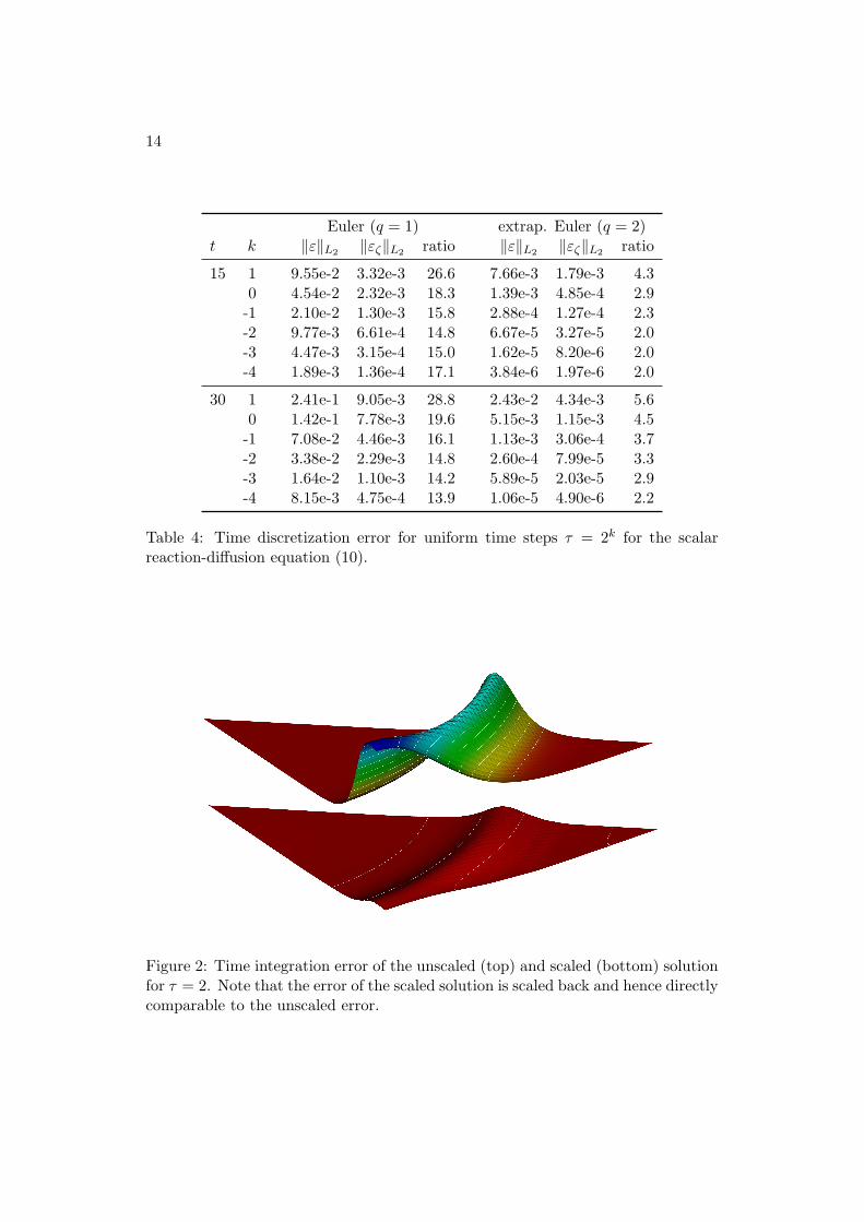
Figure 2: Time integration error of the unscaled (top) and scaled (bottom) solutionfor τ = 2. Note that the error of the scaled solution is scaled back and hence directlycomparable to the unscaled error.

15

is somewhat smaller when the reaction fronts merge and the solution shape differssignificantly from a travelling wave.

The picture is less clear for the second order scheme. Smaller gains are observed,and the deterioration with smaller time steps is more pronounced.

5 Scaling for Spatio-Temporal Discretization

Focusing on spatial or time discretization alone is bound to be suboptimal whenwe are interested in the accuracy of the integration of a reaction-diffusion equationinvolving simultaneous discretization in time and space. In the following we willcombine the error and complexity models from sections 3 and 4 above into a jointoptimization problem for designing nonlinear scalings.

We assume that the spatial and temporal error densities add up, whereas the workis combined multiplicatively:

eζ = exζ + etζ and W = WxWt

We focus on adaptive methods and therefore presume spatial error equilibration(exζ ≡ c) as well as equilibration of spatial discretization and propagation errors(‖exζ‖L2(Ω) = ‖etζ‖L2(Ω)). Inserting (5) and (12) and dropping all constant factorsthat do not affect the minimizer, we end up with the optimization problem

minζ∈Z

(∫ b

a

∣∣∣ϑ′(wζ)w(p+1)ζ

∣∣∣ dp+1

dx

)(∫ b

a

(ϑ′(wζ)w

(p+1)ζ

)2dx

)+α

2‖ζ(s)‖2L2([0,1])

to be solved for the optimal scaling ζ.

5.1 Numerical Example

Here we study the effect of nonlinear scaling of rotating spiral waves in an excitablemedium. We employ the particularly simple Barkley model [3]

u = κ∆u+ ε−1u(1− u)(u− v + b

a

)v = u− v

(15)

on Ω = [−0.5, 0.5]2 with homogeneous Neumann boundary conditions. With ε =0.01, κ = 0.002, a = 0.8, b = 0.01, and the initial values u0(x) = tanh(5r)φ(α),v0(x) = tanh(5r)φ(α+.5) for x = r(cosα, sinα), r > 0 with φ(α) =

∑i∈Z e

−2(α+2iπ)2 ,the system develops a rotating spiral wave shown in Fig. 3. The small value of εleads to a fast dynamic in u compared to v. The small value of κ subsequentlyresults in small spatial scales in u. Thus, the dominant discretization error in both,

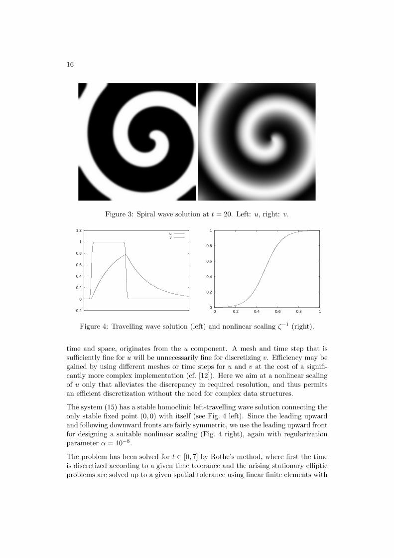
16

Figure 3: Spiral wave solution at t = 20. Left: u, right: v.

-0.2

0

0.2

0.4

0.6

0.8

1

1.2uv

0

0.2

0.4

0.6

0.8

1

0 0.2 0.4 0.6 0.8 1

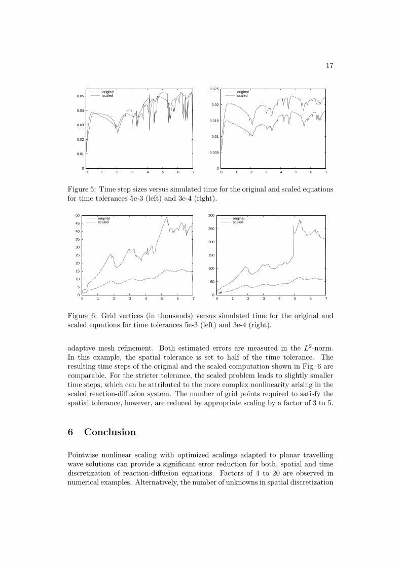
Figure 4: Travelling wave solution (left) and nonlinear scaling ζ−1 (right).

time and space, originates from the u component. A mesh and time step that issufficiently fine for u will be unnecessarily fine for discretizing v. Efficiency may begained by using different meshes or time steps for u and v at the cost of a signifi-cantly more complex implementation (cf. [12]). Here we aim at a nonlinear scalingof u only that alleviates the discrepancy in required resolution, and thus permitsan efficient discretization without the need for complex data structures.

The system (15) has a stable homoclinic left-travelling wave solution connecting theonly stable fixed point (0, 0) with itself (see Fig. 4 left). Since the leading upwardand following downward fronts are fairly symmetric, we use the leading upward frontfor designing a suitable nonlinear scaling (Fig. 4 right), again with regularizationparameter α = 10−8.

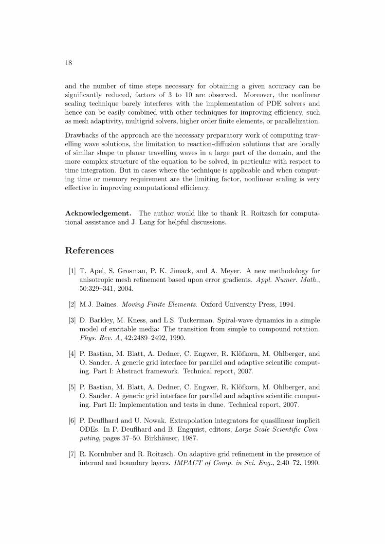
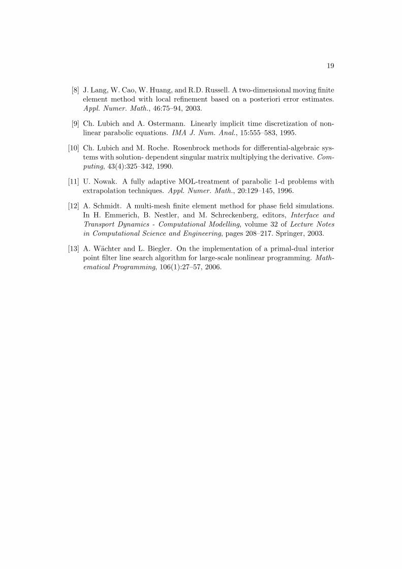
The problem has been solved for t ∈ [0, 7] by Rothe’s method, where first the timeis discretized according to a given time tolerance and the arising stationary ellipticproblems are solved up to a given spatial tolerance using linear finite elements with

17

0

0.01

0.02

0.03

0.04

0.05

0 1 2 3 4 5 6 7

originalscaled

0

0.005

0.01

0.015

0.02

0.025

0 1 2 3 4 5 6 7

originalscaled

Figure 5: Time step sizes versus simulated time for the original and scaled equationsfor time tolerances 5e-3 (left) and 3e-4 (right).

0

5

10

15

20

25

30

35

40

45

50

0 1 2 3 4 5 6 7

originalscaled

0

50

100

150

200

250

300

0 1 2 3 4 5 6 7

originalscaled

Figure 6: Grid vertices (in thousands) versus simulated time for the original andscaled equations for time tolerances 5e-3 (left) and 3e-4 (right).

adaptive mesh refinement. Both estimated errors are measured in the L2-norm.In this example, the spatial tolerance is set to half of the time tolerance. Theresulting time steps of the original and the scaled computation shown in Fig. 6 arecomparable. For the stricter tolerance, the scaled problem leads to slightly smallertime steps, which can be attributed to the more complex nonlinearity arising in thescaled reaction-diffusion system. The number of grid points required to satisfy thespatial tolerance, however, are reduced by appropriate scaling by a factor of 3 to 5.

6 Conclusion

Pointwise nonlinear scaling with optimized scalings adapted to planar travellingwave solutions can provide a significant error reduction for both, spatial and timediscretization of reaction-diffusion equations. Factors of 4 to 20 are observed innumerical examples. Alternatively, the number of unknowns in spatial discretization

18

and the number of time steps necessary for obtaining a given accuracy can besignificantly reduced, factors of 3 to 10 are observed. Moreover, the nonlinearscaling technique barely interferes with the implementation of PDE solvers andhence can be easily combined with other techniques for improving efficiency, suchas mesh adaptivity, multigrid solvers, higher order finite elements, or parallelization.

Drawbacks of the approach are the necessary preparatory work of computing trav-elling wave solutions, the limitation to reaction-diffusion solutions that are locallyof similar shape to planar travelling waves in a large part of the domain, and themore complex structure of the equation to be solved, in particular with respect totime integration. But in cases where the technique is applicable and when comput-ing time or memory requirement are the limiting factor, nonlinear scaling is veryeffective in improving computational efficiency.

Acknowledgement. The author would like to thank R. Roitzsch for computa-tional assistance and J. Lang for helpful discussions.

References

[1] T. Apel, S. Grosman, P. K. Jimack, and A. Meyer. A new methodology foranisotropic mesh refinement based upon error gradients. Appl. Numer. Math.,50:329–341, 2004.

[2] M.J. Baines. Moving Finite Elements. Oxford University Press, 1994.

[3] D. Barkley, M. Kness, and L.S. Tuckerman. Spiral-wave dynamics in a simplemodel of excitable media: The transition from simple to compound rotation.Phys. Rev. A, 42:2489–2492, 1990.

[4] P. Bastian, M. Blatt, A. Dedner, C. Engwer, R. Klofkorn, M. Ohlberger, andO. Sander. A generic grid interface for parallel and adaptive scientific comput-ing. Part I: Abstract framework. Technical report, 2007.

[5] P. Bastian, M. Blatt, A. Dedner, C. Engwer, R. Klofkorn, M. Ohlberger, andO. Sander. A generic grid interface for parallel and adaptive scientific comput-ing. Part II: Implementation and tests in dune. Technical report, 2007.

[6] P. Deuflhard and U. Nowak. Extrapolation integrators for quasilinear implicitODEs. In P. Deuflhard and B. Engquist, editors, Large Scale Scientific Com-puting, pages 37–50. Birkhauser, 1987.

[7] R. Kornhuber and R. Roitzsch. On adaptive grid refinement in the presence ofinternal and boundary layers. IMPACT of Comp. in Sci. Eng., 2:40–72, 1990.

19

[8] J. Lang, W. Cao, W. Huang, and R.D. Russell. A two-dimensional moving finiteelement method with local refinement based on a posteriori error estimates.Appl. Numer. Math., 46:75–94, 2003.

[9] Ch. Lubich and A. Ostermann. Linearly implicit time discretization of non-linear parabolic equations. IMA J. Num. Anal., 15:555–583, 1995.

[10] Ch. Lubich and M. Roche. Rosenbrock methods for differential-algebraic sys-tems with solution- dependent singular matrix multiplying the derivative. Com-puting, 43(4):325–342, 1990.

[11] U. Nowak. A fully adaptive MOL-treatment of parabolic 1-d problems withextrapolation techniques. Appl. Numer. Math., 20:129–145, 1996.

[12] A. Schmidt. A multi-mesh finite element method for phase field simulations.In H. Emmerich, B. Nestler, and M. Schreckenberg, editors, Interface andTransport Dynamics - Computational Modelling, volume 32 of Lecture Notesin Computational Science and Engineering, pages 208–217. Springer, 2003.

[13] A. Wachter and L. Biegler. On the implementation of a primal-dual interiorpoint filter line search algorithm for large-scale nonlinear programming. Math-ematical Programming, 106(1):27–57, 2006.