5. diffusion/reaction application
TRANSCRIPT

125
5 DiffusionReaction Application
Diffusion of the reactants from the surface of the catalyst to the interior of its pores
constitutes one of the resistances in a reaction system catalyzed by the solid surface In
reactor modeling for the reactions with strong diffusion limitations simplified approaches
are selected as described in the Problem Statement The most frequently used
simplifications may be illustrated as the Figure 51 for the endothermic reactions
CA
and T T
CA
T
CA
Pellet
(a) (b)
CA
and T T
CA
T
CA
Pellet
(a) (b)
Figure 51 Illustration of reactor modeling simplifications for endothermic reactions
as (a) isothermal particle and (b) uniform and symmetric distributions (re-produced from
Levenspiel 1972)
Isothermal particle where temperature is constant throughout the particle can be
illustrated as Figure 51(a) The uniform and symmetric temperature and composition
distributions can be sketched as Figure 51(b) These simplifications with the main
assumptions such as the usage of lumped transport parameters would be preferable for the
high N tubes However for the low N tubes where the presence of tube wall has an effect
on the large proportion of the entire particles these simplifications and assumptions
would be misleading regarding the strong temperature gradient due to the wall heat flux
Therefore the objective of this part was to improve the understanding of intra-particle
DiffusionReaction Application 126
transport phenomena by explicitly including conduction species diffusion and reaction
with realistic 3D external flow and temperature fields Regarding the different particle
activity levels as described in Chapter 1 two different endothermic reactions were
considered MSR and PDH
51 Model development
Two types of WS models were selected for this study a full cylinders packing was
used as the generic model and a 4-hole cylinders packing to represent the commercial
interest The models were re-meshed to implement prism layers on the external and
internal surfaces of the particles including the tube wall The fluid side prism structure
was the one used in Case-c described in section 4112 and the solid side prism layers
covered at least 3 of the particle radius from the surface The mesh specifications for
full cylinders and 4-hole cylinders packing were given in Appendix 4
The total model sizes were found to be 203 x106 cells for the full cylinders model and
346 x106 cells for the 4-hole cylinders The grid structures of full cylinders and 4-hole
cylinders models are shown in Figures 52 and 53 respectively
Figure 52 Grid structure of full cylinders model and enlarged view of an arbitrary
section
DiffusionReaction Application 127
Figure 53 Grid structure of 4-hole cylinders model and enlarged view of an arbitrary
section
In Figure 52 the top plane view mesh structure is shown where the fluid cells were
colored by red and solid cells colored by black An arbitrary section was enlarged to
represent the prism structure in fluid and solid in detail In Figure 53 the middle plane
view mesh structure is shown In the enlarged view the fluid cells were removed to make
the view clear
In order to enable the intra-particle transport processes the catalyst particles were
converted into the porous structure from solid which was the default setting and used for
the particles in the previous part of this work FLUENT defines additional surface walls
which covers the solid volumes So once the solid volumes were converted into porous
those surface walls had to be converted into interior surfaces This was a necessity
because the solid walls are impermeable so they would prevent the species transport
takes place between the pellet and the bulk fluid Note that in heterogeneous reactions
the three main mechanisms may be described as the adsorption of the reactants from the
bulk fluid on the pellet reaction and desorption of the products to the bulk fluid
FLUENT essentially considers the porous structure as a fluid zone Porous media are
modeled by the addition of a momentum source term to the standard fluid flow equations
The porous model allows setting additional inputs to model porous region including the
DiffusionReaction Application 128
porosity value and velocity field information in the region The porosity value was set to
044 as Hou and Hughes (2001) used for the steam reforming catalyst Additionally the
velocity components were fixed and set to zero in the porous media to create a
comparable pellet structure with the solid particles
The simulations were first run to determine an initial isothermal constant-composition
flow solution in the segment with periodic top and bottom conditions This flow field was
used subsequently to perform the energy and species solution in the non-periodic domain
It was observed that the changes in the flow field had minor effects on the reaction rates
when the momentum and turbulence iterations were included to the energy and species
iterations (Dixon et al 2007)
The RNG κ-ε turbulence scheme was selected with EWT and the SIMPLE pressure-
velocity coupling algorithm with the first order upwind scheme was utilized The
convergence was monitored by the pressure drop value for the flow runs and checking
the energy balance and the reaction rates in the test particle for energy and species
simulations in addition to the residuals The computations were carried out on a Sun
Microsystems SunFire V440 with 4 x 10⁶ GHz processors
511 MSR operating conditions
The same reactor conditions and fluid properties were used here as given in Table 31
Since the particles were converted into porous the thermal conductivity of the pellets was
set as 1717 wm-K to obtain the effective thermal conductivity as 10 wm-K (as given in
Chapter 3 for alumina) accounting for the pellet porosity The other pellet properties were
the same as given in Chapter 3
Species transport in the porous pellets was modeled by effective binary diffusivities
calculated from straight-pore Knudsen and molecular diffusion coefficients and corrected
using pellet porosity and tortuosity The details of these hand calculations are given in
Appendix 5(a) The dilute approximation method based on the Fickrsquos law was selected
and diffusive flux values were calculated according to equation (125) by FLUENT The
DiffusionReaction Application 129
hand-calculated effective diffusivity values for each species given in the Appendix 5(a)
are defined as Dim values Actually the multi-component method was additionally tested
by defining the binary diffusivities Dij and no significant difference was observed in the
results Therefore the results shown in the next sections for MSR reaction were obtained
by the dilute approximation method
512 PDH operating conditions
The reactor conditions and the fluid properties are given in Table 51 The inlet mass
fractions were 090 for C3H8 005 for C3H6 and 005 for H2
The pellet properties were same as for the MSR particles The diffusivities were
calculated with the same procedure as the MSR calculations and the values are given in
the Appendix 5(b) For this reaction there were differences in the results for dilute
approximation and multi-component methods and therefore both results were represented
in the relevant section
Table 51 Reactor conditions and fluid properties for PDH reaction
Tin qwall P ρ cp kf micro
[K] [kWm2] [kPa] [kgm
3] [JkgK] [WmK] [Pas]
87415 20 0101 18081 218025 00251 80110-6
52 Introducing MSR diffusionreaction
A used-defined code was created to describe the sinkssource terms in the catalyst
particles In the user-defined code the species sourcesinks terms were defined as the
following
iiiiSiSpecies MrrrS )( 332211 αααρ ++equiv ( 51 )
DiffusionReaction Application 130
where αij represents the stoichiometric coefficient of component i in the reaction j For
example for the reactions I II and III as given in equations (172) (173) and (174) the
stoichiometric coefficients for CH4 are
αCH4I = -10 αCH4II = 00 αCH4III = -10
Whereas the stoichiometric coefficients for H2 are
αH2I = 30 αCH4II = 10 αCH4III = 40
The heat generation by the reactions was calculated by the same method as described
in equation (44) As in the previous user-defined code the code must return back to the
main code the derivatives of the source terms with respect to the dependent variables of
the transport equation which are the mass fractions of the species and temperature in this
case The algorithm of the species sourcesinks calculations is shown in Figure 54
start
constants
reaction rate (kj)equilibrium (Kj)Heat of reactions (∆Hj)
getcell temperature (cell_T)cell pressure (cell_P)mass fractions (yi)
cell centroid coordinates
calculateMole fractionsPartial pressures
cell_Tle500 (K)
YES
NO
no application
go to the next cell
calculatekj(T) Kj(T) rj(T)
Source (s) =ρsΣαijrj
return(dsdyi)
to Fluent
are there any
other
cells
YES
end
NO
calculatesource derivative
(dsdyi)
Figure 54 The algorithm for the species sinkssource calculations for diffusion
reaction application
DiffusionReaction Application 131
The steps of the algorithm shown in Figure 54 were similar to the ones shown in
Figure 413 One of the major differences was the mole fractions were not constant here
and they were calculated with the mass fractions that were obtained from the main
computational domain by the code The code has 5 sub-codes corresponding to energy
term and the terms for each species except the one with the largest mass fraction Since
the mass fraction of species must sum to unity the Nth
mass fraction was determined by
N-1 solved mass fractions When the species transport is turned on in the main
computational domain of FLUENT a list of the constituent species can be entered as
fluid mixture One has to keep in mind that the order of the species in that list is
important FLUENT considers the last species in the list to be the bulk species Therefore
the most abundant species that is the one with the largest mass fraction must be set as
the last one in the list (Fluent 2005) In the MSR case this is water (H2O)
The heat generation algorithm was similar to the species sinkssource one The
differences were the source calculation where equation (51) was used instead of
equation (44) and the derivative terms which were based on the temperature not species
mass fractions The code is given in Appendix 3(c)
53 MSR diffusionreaction application results
The full cylinders and 4-hole cylinders WS models were used for the MSR reaction
implementation
531 Full cylinders model
First the flow results were obtained and compared to those from the solid particle
model Then the reactiondiffusion application was done
DiffusionReaction Application 132
5311 Flow simulation
To solve the momentum and turbulence equatios the URFrsquos at 005 less than the
default values were used The flow pathlines released form the bottom surface for the
porous particle model is shown in Figure 55(a) The pathlines are used to illustrate the
flow for tube inlet conditions and show the deflection of the flow around the porous
regions Flow features such as regions of backflow and jet flow correspond to those in
solid particle model shown in Figure 55(b)
(a) (b)(a) (b)
Figure 55 The flow pathlines released from bottom and colored by velocity
magnitude (ms) for (a) porous particle model (b) solid particle model
Additionally middle plane velocity magnitude contours are shown in Figure 56(a) and
56(b) for porous particle and solid particle models respectively The porous particle
settings created very similar results to the solid particle simulations
A quantitative comparison may be carried out by considering the radial profiles of
axial velocities for both porous and solid particle models which is shown in Figure 57
Note that the velocity profiles for both cases were almost same These results confirmed
that the change in treatment of the particles did not induce any significant changes in the
simulations
DiffusionReaction Application 133
(a) (b)(a) (b)
Figure 56 The middle-plane view velocity magnitude contours (ms) for (a) porous
particle model (b) solid particle model
0
1
2
3
4
5
0 02 04 06 08 1rrt
axia
l velo
city (m
s)
Porous Particle Solid Particle
0
1
2
3
4
5
099 0992 0994 0996 0998 1
0
1
2
3
4
5
0 02 04 06 08 1rrt
axia
l velo
city (m
s)
Porous Particle Solid Particle
0
1
2
3
4
5
099 0992 0994 0996 0998 1
Figure 57 Radial profiles of axial velocities for porous and solid particle models
DiffusionReaction Application 134
5312 Energy and species simulation
The energy and species balance equations were solved with URFrsquos of 005 less than
default values For the converged solution the residuals plot the methane consumption
rate for particle 2 and the heat balance plots are given in Appendix 6(a)
The diffusionreaction implementation may be investigated by the variations of the
temperature and species on the test particle surface and inside of the particle by the radial
profiles obtained for the entire model and by the reaction engineering parameter
effectiveness factor
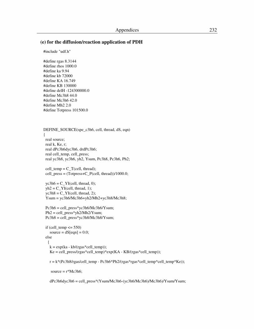
Particle surface variations As a test particle the particle number 2 surface
temperature contours with the real position of the particle in the bed and the open form
of the surface are shown in Figures 58(a) and 58(b) respectively The hotter spot on the
front section of the particle 2 can be noticed as a result of the wall heat transfer The open
form of the particle 2 surface shows the significance of the wall heat transfer in a better
way The back surface of the particle 2 was 50 degrees colder than the front surface As a
result of the endothermic effects of the reactions the lower surface temperatures have to
be expected than the bulk fluid value (82415 K) However the tube wall heat transfer
over-compensated for the endothermic effects of the reactions on the surfaces closest to
the tube wall which resulted in the hotter sections
The cooler sections of the back surface may also be related to the relatively increased
velocity field as shown in Figure 57 at rrtasymp040 This particular radial position
corresponds to the back of particle 2 and the heat transfer rate between the bulk phase
and the particles in that region may be interrupted by the high velocity flow convection
The local deviations on the particle 2 side surface are further shown for CH4 and H2
mass fractions in Figure 59 As can be noticed the depletion in CH4 results in the
production in H2 The local circular region which showed methane mass fraction minima
and corresponding hydrogen mass fraction maxima at the S=003 m must be related to
the vertex type of flow feature which occurred on that part of the surface
DiffusionReaction Application 135
(a) (b)
S [m]
-001
0
001
Z [
m]
800805810815820825830835840845850855
(a) (b)
S [m]
-001
0
001
Z [
m]
800805810815820825830835840845850855
S [m]
-001
0
001
Z [
m]
800805810815820825830835840845850855
Figure 58 The full cylinders particle 2 surface temperature contours (K) for (a) the
position of the particle in the bed (b) the open form of the surface
-001
0
001
0189
0190
0191
0192
0193
0194
0195
0196
-003 -002 -001 0 001 002 003
-001
0
001
0001
0002
0002
0003
0003
0004
0004
S [m]
Z [
m]
Z [
m]
CH4
H2
-001
0
001
0189
0190
0191
0192
0193
0194
0195
0196
-003 -002 -001 0 001 002 003
-001
0
001
0001
0002
0002
0003
0003
0004
0004
S [m]
Z [
m]
Z [
m]
-001
0
001
0189
0190
0191
0192
0193
0194
0195
0196
-003 -002 -001 0 001 002 003
-001
0
001
0001
0002
0002
0003
0003
0004
0004
S [m]
Z [
m]
Z [
m]
CH4
H2
Figure 59 The full cylinder particle 2 side surface mass fraction contours for CH4 and
H2
The intra-particle variations To investigate the intra-particle variations the same
vertical planes as used in Chapter 4 were utilized here and shown in Figure 510(a)
DiffusionReaction Application 136
In the figure the radial center of the planes were scaled as the origin and the two ends
as rrp=-10 and rrp=+10 where r is the radial position in the particle and rp is the
particle radius In the axial direction the origin was set to the lower corners and the
particle relative height was scaled as LLp=10 where L is the axial position in the
particle and Lp is the particle length
Plan
e Pl
ane
Plan
e Pl
ane
1111
Plane Plane Plane Plane
2222
Plan
e Pl
ane
Plan
e Pl
ane
1111
Plane Plane Plane Plane
2222
Plan
e Pl
ane
Plan
e Pl
ane
1111
Plane Plane Plane Plane
2222
Plane 1
rrp = -10 rrp = +1000
Plane 2
rrp = -10 00 rrp = +10
LLp = 00
LLp = 10
(a) (b)
Plan
e Pl
ane
Plan
e Pl
ane
1111
Plane Plane Plane Plane
2222
Plan
e Pl
ane
Plan
e Pl
ane
1111
Plane Plane Plane Plane
2222
Plan
e Pl
ane
Plan
e Pl
ane
1111
Plane Plane Plane Plane
2222
Plane 1
rrp = -10 rrp = +1000
Plane 2
rrp = -10 00 rrp = +10
LLp = 00
LLp = 10
Plane 1
rrp = -10 rrp = +1000
Plane 2
rrp = -10 00 rrp = +10
LLp = 00
LLp = 10
(a) (b)
Figure 510 (a) Visual planes to investigate the intra-particle variations and (b) the
temperature contours on those planes for full cylinders model
At the rrp=-10 of the plane 1 which is the closest section of the particle to the tube
wall the temperature was very high Note that this high temperature region was not on
the axial center LLp=050 of the particle This is because of the rotated position of the
particle and as a result of this rotation the lower end of the particle was closest to the
tube wall For the other positions on the plane 1 the temperature did not vary so much
For the entire plane 2 approximately 10 degrees of temperature variation was observed
Although we have shown the intra-particle temperature variation with the reaction heat
effects approximation method (Figure 415) different intra-particle temperature fields
were observed in Figure 510(b) If we compare the plane 1 contours the hotter spots can
be seen in both figures with qualitative and quantitative differences Although in Figure
415 the contours were given for different activity levels which affected the magnitude of
DiffusionReaction Application 137
the temperature the hotter spot was located on the lower corner for every activity level
However it was located at slightly higher position along the particle length for the
contours obtained by the diffusionreaction application approach Additionally on the
hotter spots relatively lower temperature value was observed by the diffusionreaction
application method These observations can be related to the methodologies behind the
two approaches The approximation method considers the uniform activity closer to the
surface of the particle and intra-particle temperature field is calculated with the constant
bulk fluid species concentration values On the other hand the activity in
diffusionreaction application is defined by the physics and temperature and species
concentrations are calculated based on that Obviously considering the bulk species
concentrations in the pellet and setting the constant activity in the approximation method
creates a higher intra-particle temperature field for the reaction to proceed However if
the concentrations are calculated according to the temperature filed reaction again
proceeds to reduce the reactants and therefore reduce the intra-particle temperatures In
the diffusionreaction application method the hotter spot was seen only at the closer point
of the particle to the tube wall However in the approximation method the hotter spot on
the lower corner of the particle was due to the combined effect of activity set on the side
and on the bottom surfaces The same effect was not seen on the top corner as standing
relatively far from the tube wall
As the benefit of diffusionreaction application the intra-particle species variations
could also be investigated Regarding the same visual planes the CH4 and H2 mass
fraction contours are shown in Figure 511
As a result of the high temperature and corresponding reaction rate a strong depletion
of methane near the tube wall was observed in plane 1 contours of Figure 511
Accordingly the increased hydrogen production was noticed on the same region More
uniform species distributions were observed in plane 2 contours as a consequence of very
reduced near wall effects
DiffusionReaction Application 138
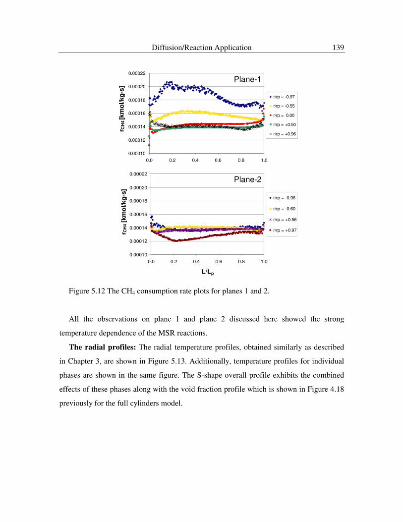
A more quantitative comparison can be obtained from the plots of CH4 consumption
rate rCH4 which is the sum of rates of reactions I and III given in equations (172) and
(174) as shown in Figure 512
Plane-1 Plane-1
Plane-2 Plane-2
CH4 mass fraction H2 mass fraction
Plane-1 Plane-1
Plane-2 Plane-2
CH4 mass fraction H2 mass fraction
Figure 511 CH4 and H2 mass fraction contours on Plane-1 and Plane-2 for full
cylinders model
The plots show the change of CH4 consumption rate along the length of the pellet for
different radial positions As can be seen from plane 1 plot at the near wall region the
reaction rate was very high as a result of high temperature For the radial positions away
from the near wall region the rates were reduced down After the second half of the
pellet from rrp =00 to rrp =+10 the rates were almost the same
Plane 2 reaction rates were almost the same for all radial positions with the same
magnitude as the results obtained in the second half of plane 1 The main difference was
seen at rrp=+097 where the CH4 consumption rate was lower than the other radial
position results The lower temperature at that position which is shown in Figure 59(b)
created the lower reaction rates
DiffusionReaction Application 139
000010
000012
000014
000016
000018
000020
000022
00 02 04 06 08 10
LLp
r CH
4 [k
mo
lkg
-s]
rrp = -097
rrp = -055
rrp = 000
rrp = +050
rrp = +096
000010
000012
000014
000016
000018
000020
000022
00 02 04 06 08 10
LLp
r CH
4 [
km
olkg
-s]
rrp = -096
rrp = -060
rrp = +056
rrp = +097
Plane-1
Plane-2
000010
000012
000014
000016
000018
000020
000022
00 02 04 06 08 10
LLp
r CH
4 [k
mo
lkg
-s]
rrp = -097
rrp = -055
rrp = 000
rrp = +050
rrp = +096
000010
000012
000014
000016
000018
000020
000022
00 02 04 06 08 10
LLp
r CH
4 [
km
olkg
-s]
rrp = -096
rrp = -060
rrp = +056
rrp = +097
Plane-1
Plane-2
Figure 512 The CH4 consumption rate plots for planes 1 and 2
All the observations on plane 1 and plane 2 discussed here showed the strong
temperature dependence of the MSR reactions
The radial profiles The radial temperature profiles obtained similarly as described
in Chapter 3 are shown in Figure 513 Additionally temperature profiles for individual
phases are shown in the same figure The S-shape overall profile exhibits the combined
effects of these phases along with the void fraction profile which is shown in Figure 418
previously for the full cylinders model
DiffusionReaction Application 140
810
820
830
840
850
0 02 04 06 08 1rrt
T (K
)
Overall Bulk fluid Porous pellet
850
890
930
970
1010
099 0995 1
810
820
830
840
850
0 02 04 06 08 1rrt
T (K
)
Overall Bulk fluid Porous pellet
850
890
930
970
1010
099 0995 1
Figure 513 Radial temperature profiles MSR full cylinders model
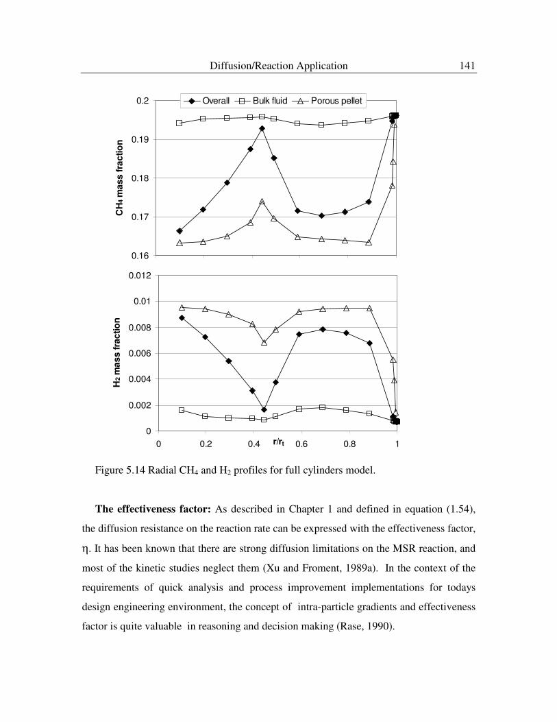
The CH4 and H2 mass fraction profiles were also obtained for the same radial positions
for which the temperature profile was obtained and are shown in Figure 514 The strong
S-shape overall CH4 profile was observed which was again strongly influenced by the
void profile The bulk fluid values did not change much from the initial values However
the overall mass fractions inside the pellet were influenced by the void fractions
especially for the radial positions of rrt asymp 040 and rrt asymp 100 where the maximum local
voidage values were observed The mirror effect can be noticed between the CH4 and H2
profiles as a result of the nature of the reactions CH4 is consumed and H2 is produced
DiffusionReaction Application 141
016
017
018
019
02
0 02 04 06 08 1rr
CH
4 m
ass f
ractio
n
Overall Bulk fluid Porous pellet
0
0002
0004
0006
0008
001
0012
0 02 04 06 08 1rrt
H2 m
ass fra
ctio
n
016
017
018
019
02
0 02 04 06 08 1rr
CH
4 m
ass f
ractio
n
Overall Bulk fluid Porous pellet
0
0002
0004
0006
0008
001
0012
0 02 04 06 08 1rrt
H2 m
ass fra
ctio
n
Figure 514 Radial CH4 and H2 profiles for full cylinders model
The effectiveness factor As described in Chapter 1 and defined in equation (154)
the diffusion resistance on the reaction rate can be expressed with the effectiveness factor
η It has been known that there are strong diffusion limitations on the MSR reaction and
most of the kinetic studies neglect them (Xu and Froment 1989a) In the context of the
requirements of quick analysis and process improvement implementations for todays
design engineering environment the concept of intra-particle gradients and effectiveness
factor is quite valuable in reasoning and decision making (Rase 1990)
DiffusionReaction Application 142
To calculate the effectiveness factor based on the definition we needed the averaged
reaction rate in the catalyst particle and the reaction rate on the particle surface For the
reaction rate inside of the particle the rates were calculated for each computational cell
and the volume averages were taken This was done by a user-defined code and it is
given in Appendix 3(d) for the particle 2 The reaction rates were then returned to
FLUENT and obtained from its user interface
For the surface reaction rate calculation the surface temperatures and species mole
fractions were exported in an ASCII file for each surface cell Using this ASCII file a
spreadsheet was prepared to calculate the reaction rates for each cell and then the area
averaged values were obtained
These calculations were carried out for the three reactions of interest and the
effectiveness factors for particle 2 were obtained by the equation (154) as
0836010219311
100195214
5
=times
times=
minus
minus
minusIIIreactionη 1622010201695
104395386
7
=times
times=
minus
minus
minusIreactionη
6072010433702
104777017
7
=times
timesminus=
minus
minus
minusIIreactionη
As can be noticed the surface reaction rates were higher than the particle reaction
rates which results in the effectiveness factors of less than unity It can also be noted that
the reaction-III is the dominant reaction as compared to the others by an order of
magnitude of the reaction rates So the low effectiveness factor for the dominant reaction
is in agreement with the industrial observations (Stitt 2005) and with the
pseudocontinuum modeling results (Pedernera et al 2003)
The reaction-II which is known as the water-gas-shift reaction (WGSR) is strongly
equilibrium limited due to the thermodynamic constraints at high temperatures
Therefore there is a strong tendency to proceed in the reverse direction The negative
reaction rate obtained for WGSR in the particle was due to this phenomenon However
the surface reaction rate was in the forward direction which implied that the CO2 and H2
diffused to the bulk fluid more easily and since the equilibrium level was not reached the
DiffusionReaction Application 143
reaction proceeded in the forward direction which resulted in a positive reaction rate
value
In order to calculate the effectiveness factors for a pellet that is not affected by the tube
wall particle number 12 was additionally considered although it was not entirely in the
model This particle is standing at the back of particle 2 at the same axial position as
shown in Figure 515
Particle 2 Particle
12
Particle 2 Particle
12
Figure 515 Particle 2 and 12 relative positions in WS model
The reaction rates for particle 12 were calculated as described above and the
effectiveness factors were found to be
1106010235451
101117314
5
=times
times=
minus
minus
minusIIIreactionη 2399010865383
102653896
7
=times
times=
minus
minus
minusIreactionη
7829010277532
107831817
7
=times
timesminus=
minus
minus
minusIIreactionη
When the effectiveness factors of particle 2 and particle 12 are compared the higher
values for the particle away from the wall can be noticed although this difference was not
too much
The wall effect on the effectiveness factor as an averaged reaction engineering
parameter may be utilized to obtain the radial effectiveness factor profiles for the entire
DiffusionReaction Application 144
model Again regarding the definition of the η we needed the surface reaction rates for
each radial position For this reason particle surface planes were created in addition to
the available visual radial planes In Figure 516(a) the previously generated radial plane
is shown at rrt = 089 as an example case where the particles were colored by red and
the fluid was colored by yellow The particle surfaces plane which is shown in Figure
516(b) for the same radial position was created considering only the outer shell
intersections of the particles at the same radial position
(a) (b)(a) (b)
Figure 516 (a) the particle and fluid regions and (b) the particle surfaces for the radial
position of rrt = 089
The temperatures and the species mole fractions were obtained from these surface
planes for each radial position and reaction rates were calculated on a spreadsheet The
obtained surface reaction rate radial profiles are shown in Figure 517 for reactions I and
III The increasing trend of the surface reaction rates can be noticed for both of the
reactions towards the tube wall where the maximum values were reached Figure 517
also represents the near wall effects on the particle surfaces which directly reflected to the
surface reaction rates Fluctuations were observed around the rrt = 040 position for both
of the reactions The reason for these changes can also be related to the local bed
voidages The reaction rates had to be calculated utilizing the temperature and species
DiffusionReaction Application 145
information for the less solid surface area in the related radial positions Therefore the
area averaged values were more sensitive to the maximum or minimum values as a result
of their contribution to the final averaged value
0000100
0000110
0000120
0000130
0000140
0000150
0000160
0000170
0000180
reaction III
0000004
0000005
0000006
0000007
0000008
0000009
0000010
0000011
0000012
0 02 04 06 08 1
rrt
reaction I
su
rfa
ce r
eac
tio
n r
ate
[km
ol
kg
-s]
0000100
0000110
0000120
0000130
0000140
0000150
0000160
0000170
0000180
reaction III
0000004
0000005
0000006
0000007
0000008
0000009
0000010
0000011
0000012
0 02 04 06 08 1
rrt
reaction I
su
rfa
ce r
eac
tio
n r
ate
[km
ol
kg
-s]
Figure 517 The surface reaction rate profiles for reactions I and III
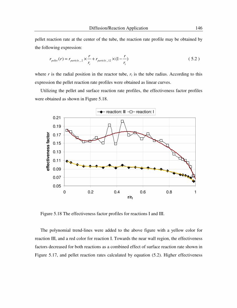
To obtain the radial effectiveness factor profiles a representation of the reaction rate
profile inside the pellets was necessary The available pellet reaction rates for particles 2
and 12 were utilized for this purpose If the particle 2 reaction rate is considered as the
pellet reaction rate closest to the wall and the particle 12 reaction rate is considered as the
DiffusionReaction Application 146
pellet reaction rate at the center of the tube the reaction rate profile may be obtained by
the following expression
)1()( 12_2_
t
particle
t
particlepelletr
rr
r
rrrr minustimes+times= ( 52 )
where r is the radial position in the reactor tube rt is the tube radius According to this
expression the pellet reaction rate profiles were obtained as linear curves
Utilizing the pellet and surface reaction rate profiles the effectiveness factor profiles
were obtained as shown in Figure 518
005
007
009
011
013
015
017
019
021
0 02 04 06 08 1
rrt
eff
ecti
ven
ess
facto
r
reaction III reaction I
Figure 518 The effectiveness factor profiles for reactions I and III
The polynomial trend-lines were added to the above figure with a yellow color for
reaction III and a red color for reaction I Towards the near wall region the effectiveness
factors decreased for both reactions as a combined effect of surface reaction rate shown in
Figure 517 and pellet reaction rates calculated by equation (52) Higher effectiveness
DiffusionReaction Application 147
factors of reaction I than reaction III were observed although they came closer in the near
wall region
The other method of obtaining the pellet reaction rate profile may be to consider the
step change in pellet reaction rates instead of setting a linear change as described above
This can be done by considering particle 12 reaction rate from 00 le rrt lt 05 and
particle 2 reaction rate for 05 le rrt le 10 as the pellet reaction rate profile Then the
effectiveness factor profiles can be obtained with the same surface reaction rate values
used above The comparison of the effectiveness factor profiles obtained by a linear and
by a step change in the pellet reaction rates is shown in Figure 519 for only the dominant
reaction
005
006
007
008
009
010
011
012
0 02 04 06 08 1
rrt
eff
ectiven
ess f
acto
r
linear change step change
Figure 519 The effectiveness factor profiles for reaction III with linear and step
change in pellet reaction rates
DiffusionReaction Application 148
As can be seen in Figure 519 the step change effect is noticeable in the center of the
model and there was not a smooth transition as in the linearly varied one However in
total the trends were quite similar in both cases
There is an order of magnitude difference observed in effectiveness factors obtained by
us and Pedernera et al (2003) where they have focused on the axial middle location of the
reactor The methodological difference was that we have utilized the realistic 3D flow
field around the explicitly positioned realistic catalyst particles and considered the
interactions between the bulk fluid and the pellets in our modeling However Pedernera
et al considered the pseudocontinuum approach to make one-dimensional particle
simulations as summarized in Chapter 2
We will make use of our effectiveness factor profile in Chapter 6 where we will
compare the results obtained in this chapter with the explicitly created pseudocontinuum
model
532 4-hole cylinder model
As in the full cylinders model simulations first the flow solution was obtained and
then the reactiondiffusion was applied
5321 Flow simulation
The flow simulation was carried out by solving the momentum and turbulence
equations as before The URFrsquos were selected as 005 less than the default values The
flow pathlines released from the bottom surface are shown in Figure 520
DiffusionReaction Application 149
Figure 520 The flow pathlines released from bottom and colored by velocity
magnitude (ms) for 4-hole model
5322 Energy and species simulation
To reach the converged energy and species simulation iterations were started with the
URF values of 005 for 3000 iterations After the residuals were flattened out the factors
were increased to 020 for 500 iterations Then they were raised to 050 for 500 iterations
more Finally the simulations were completed with the URFrsquos of 080 totally in 21000
iterations The residuals plot the methane consumption rate for particle 2 and heat
balance change during the iterations are given in Appendix 6(b)
Particle surface variations The surface temperature contour of particle 2 is shown
in Figure 521(a) for the exact location of the particle in the bed and in Figure 521(b) for
the open form of it
DiffusionReaction Application 150
Z
(b)(a)
Z
(b)(a)
Figure 521 The 4-holes particle-2 surface temperature contours (K) for (a) the
position of the particle in the bed (b) the open form of the surface
The hotter section on the particle surface for the closest point to the tube wall can be
noticed for this model in a slightly less pronounced way as compared to the full cylinders
model shown in Figure 58 The hotter section originated from the lower corner of the
particle and propagated upwards with the flow convection The related hotter region of
the particle bottom surface can be seen in the open form of the surface and mostly the
closest internal hole to that section was influenced by the wall effect This situation may
be clearly seen in Figure 522 The internal hole that was affected by the tube wall is
shown with a dashed line bordered rectangle
DiffusionReaction Application 151
(a) (b)(a) (b)(a) (b)
Figure 522 The 4-hole cylinders model particle 2 detailed view (a) bottom (b) top
Previously the flow field comparison of the models with different sizes and numbers
of internal holes was investigated (Nijemeisland 2002) and it is not the scope of our
work On the other hand to emphasize the benefit of multi-hole catalyst particles
regarding the diffusionreaction taking place in them the above observation may be
coupled to the Figure 523 where the pathlines passing through the holes of the particle 2
are shown In Figure 523(a) the pathlines are colored by the velocity magnitude which
represents the different velocity fields inside the holes whereas in Figure 523(b) they
were colored by the static temperature which shows the temperature difference of the
fluid passing through the holes The hole with the hotter surface shown in Figure 522 is
represented by the dashed lines in Figure 523 Although the velocity passing through that
hole was higher than the other holes the fluid heated up while passing through that hole
This was achieved by conduction from the inside wall of that hole to the fluid and by
convection in the fluid Ultimately these phenomena are triggered by the tube wall heat
transfer Increasing the particle fluid contact area or GSA with introducing multiple
holes and effects of transport phenomena may be further investigated by intra-particle
temperature and species variations
DiffusionReaction Application 152
(a) (b)(a) (b)(a) (b)
Figure 523 The pathlines of flow passing through the holes of particle 2 colored by
(a) the velocity magnitude (ms) and (b) the static temperature (K)
The intra-particle variations To investigate the intra-particle temperature and
species variations the 45 degree rotated versions of plane 1 and plane 2 along the particle
axis were generated as plane 3 and plane 4 which intersect the internal holes in the model
The plane 1 and plane 2 temperature contours are shown with their original positions in
Figure 524(a) and with the transformed versions in Figure 524(b)
rrp= -10 rrp= +1000 rrp= -10 rrp= +1000
LLp=00
LLp=10
Plane 1 Plane 2
Pla
ne
1
Plane
2
(a) (b)
rrp= -10 rrp= +1000 rrp= -10 rrp= +1000
LLp=00
LLp=10
Plane 1 Plane 2
Pla
ne
1
Plane
2
(a) (b)
Figure 524 (a) Visual planes 1 and 2 to investigate the intra-particle variations and (b)
the temperature contours on those planes for 4-hole cylinders model
DiffusionReaction Application 153
The maximum temperature was reached on the lower left corner of plane 1 and the
particle gradually cooled down towards the inside of it due to the reaction heat effects
The relatively cooler and hotter longitudinal patterns were seen on the planes in Figure
524(b) as a result of the contribution of the surfaces of the inner holes located close by
Additionally the CH4 and H2 mass fraction contours on the same planes are shown in
Figure 525 The strong methane depletion and hydrogen production can be noticed on the
lower left corner of the plane 1 where the higher temperature region was seen in Figure
524(b) Right after that at the position rrp asymp -05 the sudden increase in CH4 and a
decrease in H2 mass fractions were observed with a small spot on the bottom of plane 1
This position was very close to the nearest hole and plane 1 was almost intersected by
that hole Therefore the species mass fractions were influenced by the bulk fluid values
in that point Since the intra-particle temperature value at that position was similar to the
fluid temperature we have not seen a difference in the temperature contour
The plane 2 CH4 and H2 contours can be directly supported by the temperature
contours At the position of -10 lt rrp lt 00 as a result of the lower temperatures the
higher methane and lower hydrogen mass fractions were seen However the effects of
increase in temperature at 00 lt rrp lt 05 on the methane and hydrogen quantities were
noticeable
DiffusionReaction Application 154
Plane-1
Plane-2
CH4 mass fraction
Plane-1
Plane-2
H2 mass fraction
Plane-1
Plane-2
CH4 mass fraction
Plane-1
Plane-2
H2 mass fraction
Figure 525 CH4 and H2 mass fraction contours on Plane-1 and Plane-2 for 4-hole
cylinders model
The plane 3 and plane 4 temperature contours are shown in Figure 526 These planes
were created at the positions where the holes are intersected almost at their centers The
temperature difference of different holes can be seen well here as a supporting argument
to the above Fluid passing through the closest hole to the tube wall has the higher
temperature The temperature of the catalyst region closest to the tube wall was also
higher
The species distributions on planes 3 and 4 are presented in Figure 527 Note that the
scales are different in plane 3 and 4 than plane 1 and 2 in order to capture the fluid values
It was observed that the fluid region mass fractions mostly stayed at the inlet conditions
From the fluid to the pellet regions a sharp transition was noticed due to the strong
diffusion limilations
DiffusionReaction Application 155
LLp=00
LLp=10
rrp= -10 rrp= +1000 rrp= -10 rrp= +1000
Plane 3 Plane 4
(a) (b)
Pla
ne 3
Plane 4
LLp=00
LLp=10
rrp= -10 rrp= +1000 rrp= -10 rrp= +1000
Plane 3 Plane 4
(a) (b)
Pla
ne 3
Plane 4
Figure 526 (a) Visual planes 3 and 4 to investigate the intra-particle variations and (b)
the temperature contours on those planes for 4-hole cylinders model
Plane-3
Plane-4
Plane-3
Plane-4
CH4 mass fraction H2 mass fraction
Plane-3
Plane-4
Plane-3
Plane-4
CH4 mass fraction H2 mass fraction
Figure 527 CH4 and H2 mass fraction contours on Plane-3 and Plane-4 for 4-hole
cylinders model
DiffusionReaction Application 156
The radial profiles As in the full cylinders case similar radial profiles were
obtained In Figure 528 the overall (pseudohomogeneous) and fluid and solid region
temperature profiles were shown Again a similar combined effect of the fluid and solid
regions was observed on the overall profile with the local porosity influence
Additionally the overall temperature profile was lower than in the full cylinders model
as in the case of the reaction approximation discussed in Chapter 4
800
810
820
830
840
850
0 02 04 06 08 1rrt
T (
K)
Overall Fluid Solid
850
890
930
970
1010
099 0992 0994 0996 0998 1
800
810
820
830
840
850
0 02 04 06 08 1rrt
T (
K)
Overall Fluid Solid
850
890
930
970
1010
099 0992 0994 0996 0998 1
Figure 528 Radial temperature profiles MSR 4-hole cylinders model
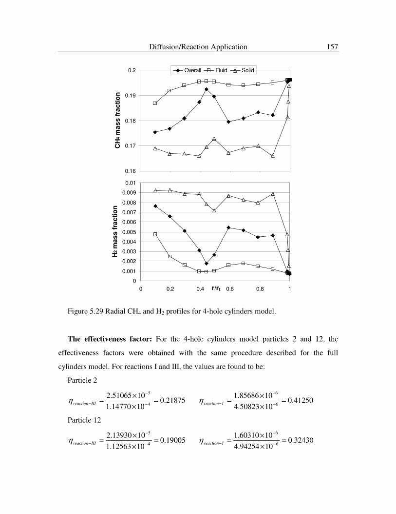
The CH4 and H2 mass fraction profiles are presented in Figure 529 Similar features
are observed in the species profiles with the full cylinders except the noticeable
difference in the overall profiles in the region 06 lt rrt lt09 The bed porosity profiles of
full and 4-hole cylinders were shown in Figure 416 and there was a significant
difference in that region the 4-hole cylinders model had a higher voidage than the full
cylinders As a result of that the fluid region compositions influenced the overall species
profiles to create higher CH4 and lower H2 contents in 06 lt rrt lt09
DiffusionReaction Application 157
016
017
018
019
02
CH
4 m
as
s f
rac
tio
n
Overall Fluid Solid
0
0001
0002
0003
0004
0005
0006
0007
0008
0009
001
0 02 04 06 08 1rrt
H2 m
as
s f
rac
tio
n
016
017
018
019
02
CH
4 m
as
s f
rac
tio
n
Overall Fluid Solid
0
0001
0002
0003
0004
0005
0006
0007
0008
0009
001
0 02 04 06 08 1rrt
H2 m
as
s f
rac
tio
n
Figure 529 Radial CH4 and H2 profiles for 4-hole cylinders model
The effectiveness factor For the 4-hole cylinders model particles 2 and 12 the
effectiveness factors were obtained with the same procedure described for the full
cylinders model For reactions I and III the values are found to be
Particle 2
21875010147701
105106524
5
=times
times=
minus
minus
minusIIIreactionη 41250010508234
108568616
6
=times
times=
minus
minus
minusIreactionη
Particle 12
19005010125631
101393024
5
=times
times=
minus
minus
minusIIIreactionη 32430010942544
106031016
6
=times
times=
minus
minus
minusIreactionη
DiffusionReaction Application 158
At a first glance we have obtained higher effectiveness factors for the front particle
than for the back particle contrary to the findings of the full cylinders model Probably
for 4-hole cylinders model particle 12 is not the best choice to consider as a
representative back particle Since particle 12 was not entirely in the model the section
where inner holes were located stayed outside of the model and we did not see the effect
of the inner holes on the surface reaction rates and ultimately on the effectiveness factors
When we compare the effectiveness factors of reaction III for 4-holes and full
cylinders models we see a 260 increase due to the 66 GSA improvement with inner
holes inclusion
54 Introducing PDH diffusionreaction application and results
The PDH diffusionreaction implementation was applied only to the full cylinders
model by the same procedure utilized in the MSR reaction application The user-defined
code created for this purpose is given in Appendix 3(e)
The flow solution was obtained for 4000 s-1
Gas Hourly Space Velocity (GHSV)
(Jackson and Stitt 2004) at steady-state condition which corresponds to the Reynolds
number of 350 based on superficial velocity and the particle diameter of a sphere of
equivalent volume to the cylindrical particle Although in general this value is quite low
to be considered as in the turbulent region the complex flow field in fixed bed reactors
has been modeled with different turbulent schemes by many researchers for even lesser
Reynolds number values (Romkes et al 2003 Guardo et al 2004) We have selected the
RNG κ-ε turbulence scheme with EWT approach for this study
The flow solution was obtained by URFrsquos of 005 less than default values and the flow
pathlines are shown in Figure 530 Relatively smooth flow features were observed as a
result of the lower superficial velocity setting
DiffusionReaction Application 159
Figure 530 Flow pathlines released from bottom and colored by velocity magnitude
(ms) for PDH reaction
The PDH diffusionreaction implementation was carried out with two different
diffusion coefficient settings as described before For the dilute approximation method
the pre-calculated Dim values were defined whereas for the M-C method the binary
diffusivities Dij were set into the materials menu of FLUENT and Dim values were
calculated by FLUENT with equation (126) The main difference in these two methods
was that the pre-calculated Dim values were obtained by us from molecular and Knudsen
diffusivities for dilute approximation method whereas the Dim values were calculated by
FLUENT from the mass fractions and binary diffusivities only for M-C method As
mentioned before these values are given in Appendix 5(b)
The diffusionreaction application results are compared for particle surface variations
intra-particle variations and effectiveness factors
Particle surface variations The test particle surface temperature contours are shown
in Figure 531 Thirty to forty degrees higher surface temperatures were obtained by the
dilute approximation method Significantly hotter sections along the particle axis were
noticed on the front of the test particle as opposed to the hotter spots seen at the lower
corner of the test particle in the MSR reaction applications
DiffusionReaction Application 160
(a) (b)(a) (b)
Figure 531 Surface temperature contours (K) obtained with the simulations by (a)
dilute approximation method and (b) M-C method
The intra-particle variations Figure 532 shows the intra-particle temperature
variation on planes 1 and 2 for both cases
Plane 1 Plane 2
(a)
(b)
Plane 1
Plane 2
Plane 1 Plane 2
(a)
(b)
Plane 1
Plane 2
Plane 1 Plane 2
(a)
(b)
Plane 1
Plane 2
Figure 532 Intra-particle temperature contours (K) on the planes 1 and 2 for the
simulations of (a) dilute approximation method and (b) M-C method
DiffusionReaction Application 161
Plane 1 temperature contours of the dilute approximation as shown in Figure 532(a)
presented a uniform axial transition throughout the particle On the other hand the intra-
particle temperature transition was different in the M-C method the corners stayed at
higher temperature but the central location in the axial direction was cooled down more
The plane 2 contours were similar and the left section of the particle was hotter than the
right section in that plane for both cases The tube wall heat transfer effect was not
expected there however due to the lower velocity observed in the fluid near to that part
of the surface which did not create a strong resistance between fluid and solid the
temperature stayed relatively closer to the bulk value
The surface and intra-particle temperatures were lower for the results obtained by the
M-S method where 80 more heat uptake was observed
(a)
(b)
Plane 1 Plane 2
(a)
(b)
Plane 1 Plane 2
Figure 533 Intra-particle C3H8 mass fraction contours on the planes 1 and 2 for the
simulations of (a) dilute approximation method and (b) M-C method
DiffusionReaction Application 162
The propane (C3H8) mass fraction contours are shown in Figure 533 for planes 1 and
2 for both cases As in the temperature contours there were significant differences for
C3H8 mass fraction qualities and quantities for both cases As a result of high intra-
particle temperatures observed for dilute approximation simulations the C3H8
consumption rate was high and lower mass fractions were observed in most of the
particle The reaction mostly took place in the outer region of the particle therefore a
sudden change was seen in that region The near wall effect was noticed in the particle
close to the tube wall along the particle axis in plane 1 The M-C method simulation
results on the other hand were quite different and lower C3H8 consumption rate was
observed which resulted in higher C3H8 mass fraction contours on both planes The
reaction took place inside of the particle not in the outer shell which presented the higher
activity level of the particle with M-C method Additionally a more uniform C3H8
distribution was seen with the simulations carried out with M-C diffusion method
Plane 1 Plane 2
(a)
(b)
Plane 1 Plane 2
(a)
(b)
Figure 534 Intra-particle H2 mass fraction contours on the planes 1 and 2 for the
simulations of (a) dilute approximation method and (b) M-C method
DiffusionReaction Application 163
The hydrogen production rate may be compared with the H2 contours on the same
planes for both cases As expected more hydrogen production was observed mostly in the
outer shell with the dilute approximation method Whereas the hydrogen mass fractions
were low and the particle was mostly active through its center with the M-C method
However the H2 distribution was not as uniform as the C3H8 distribution
820
840
860
880
900
920
940
960
0 02 04 06 08 1
T (
K)
Overall Fluid Solid
820
840
860
880
900
920
940
960
0 02 04 06 08 1rrt
T (
K)
(a)
(b)
820
840
860
880
900
920
940
960
0 02 04 06 08 1
T (
K)
Overall Fluid Solid
820
840
860
880
900
920
940
960
0 02 04 06 08 1rrt
T (
K)
(a)
(b)
Figure 535 Radial temperature profiles for PDH with (a) the dilute approximation
and (b) M-C method simulations
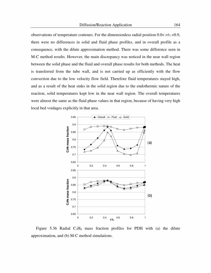
The radial profiles As shown in Figure 535(a) and (b) the dilute approximation
method temperature profiles were higher than the M-C method results as a supporting
DiffusionReaction Application 164
observations of temperature contours For the dimensionless radial position 00lt rrt lt09
there were no differences in solid and fluid phase profiles and in overall profile as a
consequence with the dilute approximation method There was some difference seen in
M-C method results However the main discrepancy was noticed in the near wall region
between the solid phase and the fluid and overall phase results for both methods The heat
is transferred from the tube wall and is not carried up as efficiently with the flow
convection due to the low velocity flow field Therefore fluid temperatures stayed high
and as a result of the heat sinks in the solid region due to the endothermic nature of the
reaction solid temperatures kept low in the near wall region The overall temperatures
were almost the same as the fluid phase values in that region because of having very high
local bed voidages explicitly in that area
065
07
075
08
085
09
095
0 02 04 06 08 1
C3H
8 m
as
s f
rac
tio
n
Overall Fluid Solid
065
07
075
08
085
09
095
0 02 04 06 08 1rrt
C3H
8 m
as
s f
rac
tio
n
(a)
(b)
065
07
075
08
085
09
095
0 02 04 06 08 1
C3H
8 m
as
s f
rac
tio
n
Overall Fluid Solid
065
07
075
08
085
09
095
0 02 04 06 08 1rrt
C3H
8 m
as
s f
rac
tio
n
(a)
(b)
Figure 536 Radial C3H8 mass fraction profiles for PDH with (a) the dilute
approximation and (b) M-C method simulations
DiffusionReaction Application 165
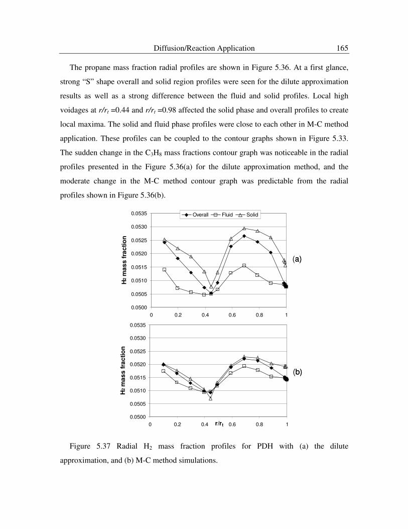
The propane mass fraction radial profiles are shown in Figure 536 At a first glance
strong ldquoSrdquo shape overall and solid region profiles were seen for the dilute approximation
results as well as a strong difference between the fluid and solid profiles Local high
voidages at rrt =044 and rrt =098 affected the solid phase and overall profiles to create
local maxima The solid and fluid phase profiles were close to each other in M-C method
application These profiles can be coupled to the contour graphs shown in Figure 533
The sudden change in the C3H8 mass fractions contour graph was noticeable in the radial
profiles presented in the Figure 536(a) for the dilute approximation method and the
moderate change in the M-C method contour graph was predictable from the radial
profiles shown in Figure 536(b)
00500
00505
00510
00515
00520
00525
00530
00535
0 02 04 06 08 1
H2 m
as
s f
rac
tio
n
Overall Fluid Solid
00500
00505
00510
00515
00520
00525
00530
00535
0 02 04 06 08 1rrt
H2 m
as
s f
rac
tio
n
(a)
(b)
00500
00505
00510
00515
00520
00525
00530
00535
0 02 04 06 08 1
H2 m
as
s f
rac
tio
n
Overall Fluid Solid
00500
00505
00510
00515
00520
00525
00530
00535
0 02 04 06 08 1rrt
H2 m
as
s f
rac
tio
n
(a)
(b)
Figure 537 Radial H2 mass fraction profiles for PDH with (a) the dilute
approximation and (b) M-C method simulations
DiffusionReaction Application 166
The hydrogen mass fraction profiles are presented in Figure 537 Similar observations
were made as for the propane mass fraction profiles and closer fluid and solid region
profiles were seen in the M-C method results As expected there was a relation between
the hydrogen contour graph and mass fraction profiles shown in Figures 534 and 537(b)
The effectiveness factor For dilute approximation method and M-C method results
the effectiveness factors were calculated for front (particle 2) and back (particle 12)
particles
The dilute approximation
2410010864364
101737413
3
2 =times
times=
minus
minus
minusparticleη 2900010231794
102288913
3
12 =times
times=
minus
minus
minusrparticleη
M-C method
6910010744432
108961713
3
2 =times
times=
minus
minus
minusparticleη 7885010668792
101044623
3
12 =times
times=
minus
minus
minusrparticleη
The higher effectiveness factors were obtained with the M-C method results than the
dilute approximation method by almost a factor of 28 The effectiveness factor values
can be coupled to the intra-particle contours and radial profile observations
To understand the reason of having different effectiveness factors with dilute
approximation and M-C method the relative sizes of the molecules must be considered
The C3H8 and C3H6 molecules are alike each other and much bigger than the H2
molecule (almost 9 times in molecular volumes) Therefore the C3H8H2 and C3H6H2
binary diffusivity values are much bigger than the C3H8C3H6 one Note that for the
dilute approximation the effective diffusivities are calculated by considering the
molecular and Knudsen diffusivities So in dilute approximation case Knudsen diffusion
dominates the effective diffusivity calculations However for the M-C method the
effective diffusivities are calculated utilizing the binary diffusivities where molecular
difference plays an important role Therefore the calculated effective diffusivities for
dilute approximation method are order of magnitude smaller than the ones calculated by
DiffusionReaction Application 167
FLUENT with only binary diffusivities as given in Table 52 As a result of this
difference higher particle effectiveness for M-C method was obtained
Table 52 Effective diffusivities used in different cases (m2s)
Dilute approximation M-C
mHCD 83 42x10
-6 82x10
-5
mHCD 63 37x10
-6 50x10
-5
mHD 2 19x10
-5 29x10
-4
Since the species molecular sizes are comparable to each other for MSR reaction
compounds there were no differences observed between the results of different
diffusivity settings and therefore only dilute approximation results were shown in the
previous section
As expressed in the PDH reaction introduction given in Chapter 1 and in the literature
overview in Chapter 2 this reaction has been mostly investigated with the coke formation
in modeling studies regarding different reactor types than the one used here to increase
the yield and conversion On the other hand this reaction has been known with the high
effectiveness factor or with the high particle activity (Jackson and Stitt 2004) and this
was the main reason that we have considered this reaction in our study to implement our
diffusionreaction application to a different activity level reaction than the MSR
Although we have not considered different features of this reaction as described above
based on our observations the M-C method may be considered as more suitable selection
for diffusive flux modeling in the PDH reaction
DiffusionReaction Application 168
55 Conclusions
The diffusionreaction implementation method has been applied to two different
reactions MSR and PDH and two different geometrical models with full and 4-hole
cylinders packings
The MSR reaction application results showed strong temperature gradients and
induced species fields within the wall particles Strong diffusion limitations affected the
temperature and species parameters to create non-symmetric and non-uniform fields All
these observations were contrary to the conventional assumptions used in reactor
modeling Based on our observations the usage of conventional modeling methods may
result in mis-evaluations of reaction rates and ultimately the design considerations may
be affected such as the mis-prediction of the tube lives
The PDH reaction was considered to study the reaction with lower diffusion
limitations Based on the different diffusion coefficient settings different particle activity
levels or effectiveness factors were obtained Regarding the larger molecular sizes of
propane and propene as compared to hydrogen the realistic diffusion modeling would be
achieved by the multi-component method where the effective diffusivities calculated by
the binary diffusion coefficients
169
6 Pseudo-continuum Modeling
The representative reactor models with valid parameters can be invaluable tools for the
decision making processes during the design and operation In real world problems on
the other hand the time constraints and economic facts force some compromise with
ideal models to establish the suitable procedures in design and operation Therefore up to
the present several types of models have been developed to satisfy the operating
conditions as summarized in Chapter 1
In reality the fixed bed reactor character is heterogeneous regarding the fluid flow
between the catalysts the transport processes between the fluid and catalyst and reaction
taking place on the catalyst pores The major flow is in the axial direction and energy
flow can be in both axial and radial directions with the influence of wall heat transfer
(Rase 1990) However due to the mentioned constraints to minimize these complexities
simplified models such as pseudo-continuum (P-C) models have been used Basic reactor
simplifications besides the presented pellet behavior in Figure 51 may be additionally
illustrated in Figure 61 for endothermic conditions
A Aacute
T
Cproduct
Creactant
A - Aacute
A Aacute
T
Cproduct
Creactant
A - Aacute
Figure 61 Basic reactor simplifications for the endothermic conditions (Re-produced
from Rase 1990)
Pseudo-continuum Modeling 170
As presented in the sketch endothermic reaction heat is removed at the center of the
tube which means that the radial gradient of temperature mostly exists on the tube wall
Because of this gradient concentration gradients will also occur
The fluid behavior is usually considered with a constant superficial velocity or with
some general smooth shape radial velocity profiles through the packed bed For large N
(tube-to-particle diameter ratio) tubes the deviation from a constant velocity is confined
to only a small fraction of the cross-section adjacent to the tube wall Whereas for the
low N tubes a substantial portion of the cross-section is affected by the wall A
representative plot is shown in Figure 62 regarding the flat correlation based and DPM
results based radial profiles of axial velocities
00
05
10
15
20
25
30
00 02 04 06 08 10rrt
VzV
0
DPM Flat Correlation
Figure 62 Radial profiles of dimensionless axial velocities for flat correlation based
and DPM results based settings
The correlation-based smooth curve was obtained from Tsotsas and Schlunder (1988)
for which the details are given in Appendix 7(a) and DPM results were from our CFD
simulation of full cylinders packing WS model Although the flat and the smooth curve
Pseudo-continuum Modeling 171
velocity profiles cannot exist with the presence of realistic packing especially for the low
N tubes the influence of the wall region is thought to be lumped into the parameters
applicable for heat and mass transfer as a conventional approach Therefore with these
lumped parameters the near-wall effects are aimed to not to be ignored by the selection
of either flat or smooth curve profiles
Our aim here was to create a best P-C model with the appropriate parameters or
correlations to obtain the profiles of the parameters and compare the energy and species
simulation results with previously obtained 3D DPM results by CFD as given in Chapter
5
61 Model development
The P-C models are basically represented by 2D partial differential equations as
summarized in Chapter 1 and numerical methods are used to reach the solution
Therefore researchers mostly create codes in different programming languages to solve
these 2D equations
Since our aim was to establish a comparative study with 3D DPM simulation results
we did not want to introduce scaling problems with the utilization of 2D P-C model
Therefore we have generated a 3D model by GAMBIT as shown in Figure 63(a) as a P-C
model with just fluid phase as in the conventional approach The 10 layers of prism
structure were implemented on the tube wall with the same features as applied in WS
models The outside of the prism region was meshed with tetrahedral UNS grid elements
of 0000762 m size Total model size was 350000 cells The mesh structure is shown
with an enlarged view of an arbitrary section in Figure 63(b) for the top surface
The ldquovelocity inletrdquo boundary condition was selected for the bottom surface and
ldquooutflowrdquo condition was applied for the top to ensure mass conservation without any
additional operating condition setting (ie temperature and composition) for the outlet As
in the WS models the side walls were set as symmetric
Pseudo-continuum Modeling 172
The energy and species simulations were performed by FLUENT 6216 with the pre-
defined velocity profile For a flat profile as in Figure 62 the constant superficial
velocity was defined for all the computational cells For the radial position dependent
curves shown in Figure 62 as smooth curve and DPM a user-defined code was prepared
to express the correlation or radial-position-dependent velocity function and defined
within each computational cell by just one momentum iteration The reason for that
iteration was not to solve the flow but to propagate the radial position dependence of the
local superficial velocities on each cell
ldquoFluidrdquo
Flow direction
(b)(a)
ldquoFluidrdquo
Flow direction
ldquoFluidrdquo
Flow direction
(b)(a)
Figure 63 3D P-C model (a) general view and (b) mesh structure
Except for the thermal conductivity the same fluid properties and reactor operating
conditions were used as given in Table 31 For the thermal conductivity we have either
used a constant effective value (ker) or a radial ker profile
62 Thermal conductivity determination
In order to obtain the most appropriate P-C model different correlations were selected
from literature to calculate and define different operating conditions and effective
Pseudo-continuum Modeling 173
transport parameters For the ker determination a separate study was carried out where
only wall heat transfer was considered and the obtained radial temperature profiles with
different velocity settings were compared to the DPM results
Case-1 The first case was to consider the constant ker value for entire domain To
calculate alternative ker values the prediction methods defined by Dixon (Dixon and
Cresswell 1979 Dixon 1988) and Bauer and Schlunder (1978a 1978b) were utilized
The details of correlations are given in Appendix 7(b) Similar values were calculated
with the both methods as 874 wm-K from Dixon and 840 wm-K from Bauer and
Schlunder
The temperature profile was obtained utilizing the flat velocity profile as shown in
Figure 62 and Dixonrsquos correlation result for the ker Figure 64 represents the comparison
of this temperature profile with the DPM result As can be seen the Case-1 temperatures
in the core of the bed were in quite good agreement whereas at the near wall region the
DPM predictions were not captured by the constant ker setting Obviously the near wall
heat transfer phenomenon was not defined in the P-C model with the constant velocity
and thermal conductivity settings
800
850
900
950
1000
1050
00 02 04 06 08 10rrt
T [K
]
DPM Case-1 Case-2
800
850
900
950
1000
1050
0990 0992 0994 0996 0998 1000
800
850
900
950
1000
1050
00 02 04 06 08 10rrt
T [K
]
DPM Case-1 Case-2
800
850
900
950
1000
1050
0990 0992 0994 0996 0998 1000
Figure 64 Radial temperature profiles based on DPM Case-1 and Case-2 results
Pseudo-continuum Modeling 174
Case-2 To be able to capture the near wall heat transfer phenomenon a smooth curve
velocity profile shown in Figure 62 was utilized instead of using flat velocity profile
This application was carried out by a user-defined code as given in Appendix 7(a) The
resulting temperature profile was also shown in Figure 64 and apparently no significant
improvement was observed From Case-1 and Case-2 results although the smooth curve
velocity profile provided a viscous damping near the wall the limiting factor seemed to
be the ker setting
Case-3 Instead of using the constant ker value the Winterberg and Tsotsas (2000)
correlation was utilized to obtain the effective thermal conductivity curve The details of
the correlation and the prepared user-defined code to define the correlation into FLUENT
are given in Appendix 7(b) Authors considered two parameters the slope parameter K1
and the damping parameter K2 in their expressions which are not agrave priori fixed but
subject to determination by comparison of the results obtained by this correlation and
available experimental data It was additionally noted that different pairs of K1 and K2
may be almost equally successful in describing the same experimental data Therefore we
have considered three different pairs of K1 and K2 and the results are shown in Figure 65
along with the DPM results The results obtained with the pair (b) captured the fluid
temperature adjacent to the tube wall however it was not successful at the dimensionless
radial position of 0900 lt rrt lt 0998 The pair (c) and DPM results were mostly in
agreement however near wall effects could not be predicted in spite of the slight
improvement as compared to Case-1 and Case-2 near wall region results The results
obtained by pair (a) were in between the other pairs
Generally the benefit of the effective thermal conductivity correlation was seen with
this application We have better results than the constant ker setting at the near wall
region and the core of the tube modeled well as expected and observed in the other
cases
Pseudo-continuum Modeling 175
The sudden temperature increase in the near wall region of DPM must be related to the
boundary layer resolution which must be coupled to the sudden damping in the DPM
velocity profile at that region as shown in Figure 62 Therefore the next step would be
the consideration of DPM velocity profile
800
850
900
950
1000
1050
00 02 04 06 08 10rrt
T [
K]
DPM Case-3(a) Case-3(b) Case-3(c)
800
850
900
950
1000
1050
0990 0992 0994 0996 0998 1000
800
850
900
950
1000
1050
00 02 04 06 08 10rrt
T [
K]
DPM Case-3(a) Case-3(b) Case-3(c)
800
850
900
950
1000
1050
0990 0992 0994 0996 0998 1000
Figure 65 Radial temperature profiles based on DPM and Case-3 results
Case-4 The DPM velocity profile was exactly reproduced by polynomial functions
and set into FLUENT by a user-defined code which is given in Appendix 7(a) Similarly
three different pairs of K1 and K2 were considered and the obtained temperature profiles
are shown in Figure 66
The results obtained by the pair (b) captured the fluid temperature adjacent to the tube
wall and better temperature values were seen in 0900 lt rrt lt 0998 as compared to the
Case-3 The maximum deviation was less than 40 degrees at rrt = 0997 On the other
hand pair (c) captured the near wall temperatures very well up to rrt = 0997 However
at rrt = 0999 80 degrees difference was observed with the DPM results Pair (a) can be
Pseudo-continuum Modeling 176
considered as one of the optimum profiles to compensate for the deviations mentioned for
pairs (b) and (c)
Additionally at rrt = 09 a slight disagreement was noticed between the DPM and all
the pair results In spite of that the most representative temperature profiles were
obtained utilizing the DPM-fitted velocity profile and the ker profile
800
850
900
950
1000
1050
00 02 04 06 08 10rrt
T [K
]
DPM Case-4(a) Case-4(b) Case-4(c)
800
850
900
950
1000
1050
0990 0992 0994 0996 0998 1000
Figure 66 Radial temperature profiles based on DPM and Case-4 results
63 P-C modeling for MSR reaction
The MSR reaction was introduced in P-C modeling with a similar user-defined code as
was utilized in DPM simulations with sourcesinks terms to express the effects of
reaction on temperature and species quantities The important difference in P-C modeling
was that these sourcesinks terms were considered for the entire fluid domain and the
calculations incorporated the pseudo-solid phase by the bed voidage term [1-ε(r)] in the
sourcesinks terms as expressed below for the energy and species balance equations
Pseudo-continuum Modeling 177
[ ])(1)(1
2
2
rrHr
T
rr
Tk
z
Tcu ABerps εηρρ minus∆minus=
part
part+
part
partminus
part
part ( 61 )
[ ])(11
2
2
rrr
C
rr
CD
z
Cu ABers εηρ minus=
part
part+
part
partminus
part
part ( 62 )
The right hand side of the equations (61) and (62) is the sourcesinks term which was
defined by a user-defined code Additionally we have introduced another term
effectiveness factor η in our P-C model to express the diffusion limitations As a
reminder from DPM simulations we have obtained different effectiveness factor values
for front (number 2) and back (number 12) particles as well as the effectiveness factor
profile as shown in Figure 518 We have used all three of them separately in this part of
the work to make a comparison
The effective diffusivity (Der) values were calculated form correlations provided by
Specchia et al (1980) Bauer and Schlunder (1978a 1978b) and Rase (1990) and found
to be 0002150 0005659 and 0007485 m2s respectively Details of these correlations
are provided in Appendix 7(c) The results were not significantly affected when these
different values were used as effective diffusivities in P-C modeling
In general the main modeling parameters can be considered as velocity effective
thermal conductivity effective diffusivity bed voidage and effectiveness factor Either
constant values or spatial functional terms are utilized for these parameters Since we
have previously investigated the velocity and ker parameters a further consideration was
carried out for the effectiveness factor and bed voidage in this section The energy and
species solutions were reached with the residuals in the order of 10-8
within a few
iterations (~20)
The effectiveness factor investigation Although the most suitable velocity and ker
settings were already seen in the previous section as the basic application in the P-C
modeling a flat velocity profile constant effective parameters and bed voidage were
utilized in this investigation For ker the value obtained from Dixon correlation for the
bed voidage the value of WS model with full cylinders packing and for the Der the one
Pseudo-continuum Modeling 178
obtained by Bauer and Schlunder correlation were utilized As a result of the energy and
species simulations the obtained overall heat uptake values (Q) tube wall temperatures
(TWT) and methane conversions (XCH4) are given in Table 61 with the DPM results to
make a comparison Equation (22) was used for the XCH4 calculations The temperature
and methane and hydrogen mass fraction profiles are presented in Figure 67
Table 61 P-C modeling results for different effectiveness factors and DPM results
η-front particle η-back particle η-profile DPM
Q [w] 2145 2885 2150 2532
TWT [K] 8362 8356 8364 10048
XCH4 [] 0356 0488 0354 0530
The DPM TWT value was not reached by any P-C model as a consequence of flat
effective thermal conductivity and axial velocity profiles Although the overall heat
uptake value of DPM was not reproduced comparable values of Q were obtained with
different effectiveness factor settings If we compare the front and back particle results
we see a reduced heat uptake as a result of lower η-front particle This can be explained
with the influence of the reduced effectiveness factor on the RHS of the equation (61)
The higher diffusion barrier due to the lower η reduces the reaction heat effect and
therefore less heat is transferred into the pseudo-positioned particles to establish the
energy balance The η-profile heat uptake value was quite similar to the η-front particle
value although the profile was obtained considering both the front and back particle
reaction rates Figure 518 shows the possible reason for this observation At the
dimensionless radial position of 085 le rrt le 100 the local effectiveness factors were
lower than the front particle values as noted in section 5312 Because of this the
reaction heat effects were reduced as compared to the ones obtained by the constant front
and back particle effectiveness factor settings in that particular position Therefore as a
result of the contribution of the reduced heat effects in that region to the total heat uptake
Pseudo-continuum Modeling 179
the higher heat effects due to the η-back particle were lost with the utilization of the η-
profile which resulted in very similar heat uptake values with the η-front particle
simulation
The DPM heat uptake value which was found to be in-between the front and back
particle results could not be obtained by the η-profile setting although the near wall
particle effectiveness was defined by that profile This situation might be understood well
when the tube wall temperatures were compared Obviously the near wall temperature
field of DPM was not reproduced by any effectiveness factor setting as a result of not
using the suitable effective thermal conductivity The temperature profiles shown in
Figure 67(a) represent this situation Actually with the parameters used in this
investigation the entire DPM radial temperature profile was not obtained We have
selected the basic and frequently addressed P-C modeling parameters and it was clear
that the DPM and P-C predictions were not in agreement
Although the reactor models that we have been considering in our studies are too short
in length to obtain a comparable conversion value with any experimental or industrial
data we have utilized the methane conversion as another control parameter for P-C
model testing It was observed that the conversion obtained with the η-back particle
simulation was the closest one to the DPM results with 8 deviation
Figures 67(b) and (c) represent the P-C modeling results of CH4 and H2 mass fractions
respectively The DPM profiles shown in the figure were only the bulk fluid mass
fractions as previously shown in Figure 514 with overall and porous pellet profiles
Since the P-C model essentially considers only the fluid region the overall or porous
pellet profiles were not the appropriate parameters to make a suitable comparison The
mass fraction profiles obtained from the P-C models with different effectiveness factors
were not in agreement with the DPM profiles and they were almost constant The lower
CH4 and higher H2 mass fractions were noticed for the η-back particle simulations as
compared to the η-front particle and η-profile results as a consequence of higher
effectiveness value
Pseudo-continuum Modeling 180
800
850
900
950
1000
1050
00 02 04 06 08 10
T [K
]
800
850
900
950
1000
1050
0990 0992 0994 0996 0998 1000
01935
01940
01945
01950
01955
01960
01965
00 02 04 06 08 10
CH
4 m
ass fra
ctio
n
00005
00007
00009
00011
00013
00015
00017
00019
00021
00 02 04 06 08 10rrt
H2 m
ass fra
ctio
n
DPM front particle back particle profile
(a)
(b)
(c)
800
850
900
950
1000
1050
00 02 04 06 08 10
T [K
]
800
850
900
950
1000
1050
0990 0992 0994 0996 0998 1000
800
850
900
950
1000
1050
00 02 04 06 08 10
T [K
]
800
850
900
950
1000
1050
0990 0992 0994 0996 0998 1000
01935
01940
01945
01950
01955
01960
01965
00 02 04 06 08 10
CH
4 m
ass fra
ctio
n
00005
00007
00009
00011
00013
00015
00017
00019
00021
00 02 04 06 08 10rrt
H2 m
ass fra
ctio
n
DPM front particle back particle profile
(a)
(b)
(c)
Figure 67 The radial profiles of (a) static temperature (b) CH4 mass fraction and (c)
H2 mass fraction obtained by the P-C model with different effectiveness factor settings
Pseudo-continuum Modeling 181
By this investigation different effectiveness factors were compared to each other and
to DPM results while considering constant effective parameters As a next step the bed
voidage correlations were considered to create radial profiles instead of using constant
values
The bed voidage parameter investigation The same velocity thermal conductivity
and effective diffusivity values were utilized as before The η-profile was applied to
define the diffusion limitations The bed voidage correlations provided by Winterberg and
Tsotsas (2000) and Bey and Eigenberger (2001) were considered In addition to these
correlations the DPM bed voidage profile was re-produced by fitted polynomial
functions and applied by a user-define code into the P-C model The details of the
correlations and the code are given in Appendix 7(d) The obtained voidage profiles are
shown in Figure 68 The DPM profile presented in the figure is the one obtained from
WS model and the reproduced one by the polynomial functions was exactly the same
0
02
04
06
08
1
0 02 04 06 08 1rrt
Bed
vo
idag
e
Winterberg amp Tsotsas Bey amp Eigenberger DPM
Figure 68 Radial bed voidage profiles obtained by the correlations and from DPM
As can be seen from the above figure none of the correlations created a representative
bed voidage profile Both of them created flat profiles at the core and an increasing trend
at the wall region The Winterberg and Tsotsas (W-T) correlation estimated very low
Pseudo-continuum Modeling 182
maxima near the wall as compared to the DPM bed voidage The Bey and Eigenberger
(B-E) correlation captured the full void region near the wall but a steep decrease was
observed for the latter part Actually the B-E correlation consists of two different
expressions for the wall and the core regions The bed voidage value at the center of the
model can be set to a higher value than the minimum which occurs radially almost at the
half of the bed By doing that a sinusoidal curve would be obtained in the core of the bed
However as can be seen in Figure 68 the minimum occurs at the core of the bed not at
rrt asymp 065 in DPM Therefore the core and the half of the bed voidage values were kept
the same which created a flat profile in the core
The P-C model results with these three different bed voidage settings were compared
to the DPM results in Table 62 for Q TWT and XCH4 values and in Figure 69 for radial
temperature and species profiles
Table 62 P-C modeling results for different bed voidages and DPM results
Winterberg amp
Tsotsas
Bey amp
Eigenberger
DPM-fitted DPM
Q [w] 2740 3297 2219 2532
TWT [K] 8359 8358 8364 10048
XCH4 [] 0450 0523 0360 0530
The heat uptake result obtained by the P-C model with W-T correlation was lower
than the one obtained by B-E correlation The higher voidage profile obtained by W-T
correlation in the core of the bed had an inductive effect on the right hand side of the
equation (61) which reduced the magnitude of the source term As a result of that the
reaction heat effects were reduced and lower Q value was reached by W-T correlation
W-T and B-E correlation models predicted 8 and 30 more heat uptake values than
the DPM result respectively whereas the value obtained by the DPM-fitted voidage
Pseudo-continuum Modeling 183
profile was lower than the DPM value by 12 On the other hand B-E correlation
predicted the closest methane conversion value to the DPM result
800
850
900
950
1000
1050
00 02 04 06 08 10
T [K
]
800
850
900
950
1000
1050
0990 0992 0994 0996 0998 1000
01935
01940
01945
01950
01955
01960
01965
00 02 04 06 08 10
CH
4 m
as
s fra
ctio
n
00005
00007
00009
00011
00013
00015
00017
00019
00021
00 02 04 06 08 10rrt
H2 m
ass f
ractio
n
DPM Winterberg amp Tsotsas Bey amp Eigenberger DPM-fitted
(a)
(b)
(c)
800
850
900
950
1000
1050
00 02 04 06 08 10
T [K
]
800
850
900
950
1000
1050
0990 0992 0994 0996 0998 1000
800
850
900
950
1000
1050
00 02 04 06 08 10
T [K
]
800
850
900
950
1000
1050
0990 0992 0994 0996 0998 1000
01935
01940
01945
01950
01955
01960
01965
00 02 04 06 08 10
CH
4 m
as
s fra
ctio
n
00005
00007
00009
00011
00013
00015
00017
00019
00021
00 02 04 06 08 10rrt
H2 m
ass f
ractio
n
DPM Winterberg amp Tsotsas Bey amp Eigenberger DPM-fitted
(a)
(b)
(c)
Figure 69 The radial profiles of (a) static temperature (b) CH4 mass fraction and (c)
H2 mass fraction obtained by the P-C model with different bed voidage settings
Pseudo-continuum Modeling 184
The TWT values and temperature profiles were different from the DPM results as
observed before
There were slight effects of the B-E correlation on the methane and hydrogen mass
fraction profiles as shown in Figure 69 (b) and (c) especially at the near wall region as a
result of the sharp damping created there Since the near wall bed voidage was not
pronounced that much with W-T correlation no significant variation was observed on the
related profiles Although the strong S-shape profiles were not captured the more
variation in the mass fraction profiles was seen for the DPM-fitted model predictions
At the end of the bed voidage parameter investigation the DPM-fitted profile was
selected for the next stage where the most representative P-C model was aimed to be
produced by considering the appropriate effective thermal conductivity and the DPM-
fitted parameters
The P-C model with DPM-fitted parameters To reproduce the averaged results of
the DPM the DPM-fitted profiles were utilized for the parameters Axial velocity and
bed voidage radial profiles were already obtained above from the DPM-fitted polynomial
functions Additionally the effective diffusivity profile was created from the DPM as
shown in Figure 610 by taking the mass fraction weighted average of each species The
blue line presented in Figure 610 was reproduced by polynomial functions and set to the
P-C model with a user-defined code which is given in Appendix 7(c)
Previously obtained effectiveness factor profile η-profile and the thermal
conductivity profile (Winterberg and Tsotsas 2000) were utilized Based on the three
different K1 and K2 pairs the obtained Q TWT and XCH4 values are given in Table 63
and the temperature and methane and hydrogen profiles are shown in Figure 611 with
the DPM results for comparison
The heat uptake values of the P-C models were close to the DPM value with 75
maximum deviation The averaged TWT was exactly re-produced by P-C (1) model
where the Q value was 53 lower than the DPM result In order to obtain a close Q
Pseudo-continuum Modeling 185
value to the DPM result the P-C (2) model was created with different K1 and K2 pairs
which increased the TWT by 100 degrees One can conclude that when the DPM Q value
was asymptotically reached in the P-C model with different K1 and K2 values the TWT
would exceed the DPM predictions by hundreds of degrees Another parameter pair was
utilized to create the P-C (3) model which predicts the lower TWT Although the TWT
predictions were strongly affected by different K1 and K2 pairs the least influence was
seen on the methane conversion predictions and the maximum deviation form DPM
prediction was found as 0082
000E+00
500E-05
100E-04
150E-04
200E-04
250E-04
0 02 04 06 08 1
rrt
Diffu
siv
ity [m
2s
]
h2 co2 ch4 h2o co Effective
000E+00
500E-07
100E-06
150E-06
200E-06
250E-06
300E-06
350E-06
400E-06
0999 09992 09994 09996 09998 1
000E+00
500E-05
100E-04
150E-04
200E-04
250E-04
0 02 04 06 08 1
rrt
Diffu
siv
ity [m
2s
]
h2 co2 ch4 h2o co Effective
000E+00
500E-07
100E-06
150E-06
200E-06
250E-06
300E-06
350E-06
400E-06
0999 09992 09994 09996 09998 1
Figure 610 The species and effective diffusivity profiles obtained from the DPM
Table 63 P-C modeling results with DPM-fitted parameters and DPM results
P-C (1) P-C (2) P-C (3) DPM
Q [w] 2398 2450 2341 2532
TWT [K] 10043 11041 8764 10048
XCH4 [] 0600 0596 0612 0530
Pseudo-continuum Modeling 186
800
850
900
950
1000
1050
1100
1150
00 02 04 06 08 10
T [K
]
800
850
900
950
1000
1050
1100
1150
0990 0992 0994 0996 0998 1000
01890
01900
01910
01920
01930
01940
01950
01960
01970
00 02 04 06 08 10
CH
4 m
ass fra
ctio
n
(a)
(b)
(c)
00005
00010
00015
00020
00025
00030
00035
00040
00 02 04 06 08 10rrt
H2 m
ass
fra
ctio
n
DPM P-C (1) P-C (2) P-C (3)
800
850
900
950
1000
1050
1100
1150
00 02 04 06 08 10
T [K
]
800
850
900
950
1000
1050
1100
1150
0990 0992 0994 0996 0998 1000
800
850
900
950
1000
1050
1100
1150
00 02 04 06 08 10
T [K
]
800
850
900
950
1000
1050
1100
1150
0990 0992 0994 0996 0998 1000
01890
01900
01910
01920
01930
01940
01950
01960
01970
00 02 04 06 08 10
CH
4 m
ass fra
ctio
n
(a)
(b)
(c)
00005
00010
00015
00020
00025
00030
00035
00040
00 02 04 06 08 10rrt
H2 m
ass
fra
ctio
n
DPM P-C (1) P-C (2) P-C (3)
Figure 611 The radial profiles obtained by the DPM-fitted P-C models
Pseudo-continuum Modeling 187
The temperature profiles shown in Figure 611(a) were almost the same for all P-C
models and were in good agreement with the DPM profile The near-wall deviation was
enlarged and the well-established TWT result was additionally seen for P-C (1) in the
figure The local deviation between the P-C (1) model prediction and the DPM profile at
0996 le rrt le 0999 was around 20 to 30 degrees and this was the best agreement for
near-wall performance among the all P-C models considered so far The over prediction
of the P-C (2) model and the under prediction of the P-C (3) model was observed at the
near wall region which can be incorporated to the TWT values
Although the increase in TWT is related to the total heat uptake as creating a driving
force between the bulk fluid and the wall temperatures to increase the heat transfer rate
which ultimately increases the heat uptake as result of the endothermicity the higher
TWT values were not reflected by the heat uptakes in the same order of magnitude This
is because the local temperature deviation between the P-C models appears only at 0996
le rrt le 1000 and the same temperature field is present for the rest
The P-C model methane and hydrogen mass fraction profiles were no different than
each other and in good agreement with the DPM profiles as shown in Figure 611(b) and
(c) When the profiles obtained here were compared to the other profiles presented in
Figures 67 and 69 a drastic difference can be noticed The reason for capturing the
DPM prediction was because of considering the DPM-fitted effective diffusivity profile
instead of the flat profiles The strong S-shape P-C model mass fraction profiles were
departing from the DPM results at the core of the bed After careful investigation this
situation was understood as an artifact created by the lower velocity field at the center of
the tube regarding the applied DPM-fitted axial velocity profile In the DPM model the
velocity profile was obtained considering the entire radial surface with both fluid and
solid regions and lower bed voidage values were obtained in the core of the bed as
presented in Figure 416(b) for the full cylinders WS model Therefore the contribution
of zero velocities from the solid region reduced the averaged velocity value In P-C
modeling when the DPM-fitted axial profile was applied the reduced velocity value at
Pseudo-continuum Modeling 188
that radial position was literally considered as a velocity field So this results in the
reduced effect of the first term given in the left hand side of the equation (62) on the
species balance Thus the diffusive flux was the only effective term to balance the source
term The lower bed voidage and higher effectiveness factors at the core of the bed
created a higher source term and as a result a higher composition difference For this
reason the higher methane consumption and higher hydrogen production were seen at
that radial position Although the effective diffusivity value at the core was an order of
magnitude higher than the one of the near wall region it was not enough to compensate
for the increase in the source term to keep the compositions unaffected
64 Conclusions
The comparative study was carried out regarding the pseudo-continuum (P-C) and
discrete packing models (DPM) Different correlations were utilized in order to express
the velocity thermal conductivity bed voidage and diffusion coefficients in the P-C
models either in the form of flat profiles (constant values) or in the form of expressions to
define the radial position dependence
It was observed that the flat or correlation-based effective parameter profiles were not
enough to express the features of the DPM in terms of heat uptakes tube wall
temperatures species conversions and radial temperature and species profiles
To create the most representative P-C model the DPM-fitted parameters were utilized
and comparable results were obtained to the DPM predictions It was seen that the
temperature profiles were very much affected by the velocity and thermal conductivity
definitions On the other hand species profiles were significantly influenced by properly
defined effective diffusivity profiles
The final conclusion would be that the pseudo-continuum models cannot fully
reproduce the DPM results due to the complex model structure which cannot be
represented by the correlations or DPM-fitted expressions in a simplified model
189
7 Conclusions and Recommendations
71 Conclusions
At the end of this written document we can evaluate our observations based on the
different phases of the research regarding the main goal that we had in our minds at the
beginning Therefore the interim conclusions reached at the end of the chapters will not
be repeated here and the observations will be expressed with a global point of view of
the research
Our objective was to investigate the interaction between the chemistry taking place in
the particle and the transport processes surrounding it for the low-N fixed bed tubes
utilizing the CFD Regarding the consequences of wall heat transfer in low-N tubes that
have been expressed in the problem statement generating the proper 3D geometry was
the first cornerstone of our work For this reason we have validated our smaller size
geometry which was selected due to the computational constraints
The pseudo-continuum type of packed bed models do not account for the actual
environment for the reacting particles and therefore almost always symmetric and
sometimes uniform temperature and species distribution is assumed inside of the pellets
In our work utilizing the benefits of the CFD the diffusionreaction has been introduced
into the pellets within the realistic 3D reactor conditions and contrary to the conventional
approach the non-symmetric and non-uniform intra-particle temperature and species
variations have been obtained for the near wall particles and extensively investigated in
detail for the first time
Furthermore it has been shown that the strong near wall gradients as observed by
discrete packing models either approximating the reaction heat effects or implementing
the diffusionreaction into the catalyst particles cannot be captured by the simplified
pseudo-continuum models
Conclusions and Recommendations 190
The significance of our observations is that utilization of the conventional simplified
methodology will definitely lead to an incorrect evaluation of the reaction rates and
consequently the design considerations such as tube wall temperature and pellet and
reactor dimensions
The strong impact of our findings must be expected on fundamental reaction
engineering by moving away from empiricism towards a more rigorous treatment of the
pellet and on the industry by preventing the tube failure and obtaining improved reaction
conversion thus having positive consequences for the plant safety and efficiency and for
pollution prevention and sustainable engineering regarding the particular importance of
methane steam reforming on the hydrogen economy
72 Recommendations
In this section we will describe some of the research areas either we have touched but
not completed and thus have not discussed in the main body of the text or came to our
attention but they were either not part of the main focus of this work or
timecomputational resources were not available to spend more effort on them
721 Particle orientation
Diffusionreaction implementation was done on the specific WS model where the test
particle was located in 45 degree rotated form close to the tube wall To answer the
question if the orientation of the test particle would be important for the near wall
transport processes we re-considered the previously created WS models with different
test particle orientations (Nijemeisland 2002) with improved mesh structure on the wall-
fluid contact areas by prism layers Additionally another WS model was generated to
consider in general all the possible basic particle placements as presented in Figure 71
The model numeration was started from two regarding the model with 45 degree rotated
test particle as WS-1
Conclusions and Recommendations 191
test
particletest
particle
test
particle
WS-2 WS-3 WS-4
test
particletest
particle
test
particle
WS-2 WS-3 WS-4
Figure 71 Different WS models
We have obtained the preliminary results for WS-4 model and surface and intra-
particle temperature variation is shown in Figure 72
Plane-1
Plane-2
Plane-1 Plane-2
Mid-plane
Mid-plane
Plane-1
Plane-2
Plane-1 Plane-2
Mid-plane
Mid-plane
Figure 72 The preliminary temperature contours of test particle model WS-4
Conclusions and Recommendations 192
We have observed similar hotter sections as seen on WS-1 model test particle surface
at the closest section to the tube wall Obviously the flow convection which takes place
between the pellet surface and the tube wall affected the particle surface temperature and
this hotter section has occurred on the upper part of the pellet
The effectiveness factors were calculated for front and back particles and less
effective particles were found than the WS-1 model
067460=particlefrontη 075600=particlebackη
Keep in mind that the back particle orientations of WS-1 and WS-4 models were also
different So these preliminary results showed that the particle orientation is important
for both front and back particles Therefore it is worth to continue with WS-2 and WS-3
models to investigate up to what extent the modeling parameters such as the tube wall
temperature and the particle effectiveness can be affected
722 Wall to wall contact points
As stated in the main body of this document before we have intentionally kept a gap
between the particle to particle and the particle to tube wall contacts so as not to face
convergence problems due to skewed elements that occur with grid generation on these
contacts
Previously N = 243 tube with 10 spherical particles was modeled with contact points
(Logtenberg et al 1999) and agreement between the empirical correlations was observed
in thermal conductivity predictions for high Re flows In the later work (Nijemeisland and
Dixon 2001) for N = 2 tube with 44 spheres the spherical particle contact points were
modeled with a ldquonear-missrdquo approach where as a first step touching particles were placed
and then the model was finalized by reducing their diameters 99-995 while keeping the
same particle central coordinates to allow a gap between them Based on the experiences
of that work the spherical packing WS model was created with 995 reduction
Conclusions and Recommendations 193
Recently the 05 overlapping spherical particle geometry was introduced (Guardo et al
2006) without any meshing detail to prevent the convergence problems
As a preliminary study 998 reduced and 05 overlapping particles were created
for spherical packing WS model with GAMBIT 2230 and many skewed cells obtained
especially for the overlapping case with UNS tetrahedral elements Figure 73 presents the
mid point-view of the models where particles are not colored The 995 reduced particle
case is also shown for comparison
WS+005WS-998WS-995 WS+005WS-998WS-995
Figure 73 The mid-plane views of spherical packing WS models with 995 and
998 reduced and 005 increased size
The overall bed voidages of these models are 04147 for WS-995 04062 for WS-998
and 03915 for WS+005 Based on our previous experiences the momentum convergence
can be achieved with very low URFrsquos for the models with highly skewed cells Thus we
have obtained the pressure drop values of WS-998 and WS+005 models with the same
operating conditions as stated before and normalized based on WS-995 model value
)()(1601 998 mPamPaLP WS =∆ minus )()(7401 005 mPamPaLP WS =∆ +
Conclusions and Recommendations 194
As can be noticed there was a dramatic difference for the overlapping model pressure
drop value Therefore further investigation would have been performed to include the
heat and mass transfer However the unreasonable temperature or species values that
were calculated and stored for the skewed cells due to their skewness of course created a
disastrous convergence problem
We have not gone through these problems in the main body of the text because our
main interest was on the cylindrical packings and there was not a convergence problem
since cylindrical particles were not touching each other or the tube wall
To solve the touching particle problem a better mesh is necessary with suitable cell
structure and significant time has to be spent to create the model Recently FLUENT
announced that the version 63 has an additional feature that polyhedral cell elements can
be used which may reduce the skewness problem that occurs by tetrahedral cells The
utilization of version 63 would be a reasonable starting point to approach the problem
and the latest version of FLUENT became available in our institution couple of months
ago
Once the touchingoverlapping particle models are created with spherical and
cylindrical packings the diffusionreaction modeling can be performed to investigate the
near wall gradients for the situation where there will be no gap between the tube wall and
the particles
723 Catalyst deactivation modeling
One of the important phenomena in catalytic reactions is the catalyst deactivation
which occurs on all catalysts either gradually or fast Among the deactivation processes
carbon formation or fouling is the frequently faced problem in many reactions including
methane steam reforming and propane dehydrogenation Fouling is the physically
covering of active sites andor the entire surface of the support by carbonaceous or
inorganic deposits Severe fouling can lead to pore plugging which cuts off access to
active regions and causes loss in activity Moderate fouling causes a steady but slower
Conclusions and Recommendations 195
decline in activity that can reach a rather steady and acceptable level for long-term
operation (Rase 1990)
For propane dehydrogenation carbon formation occurs very fast and therefore it has
been considered with the main reaction all the time Technically a carbon formation is
another reaction or reactions which can be expressed with separate reaction rates The
following reaction is known as the main carbon formation reaction in the propane
dehydrogenation
283 43 HCHC +rarr ( 71 )
The rate equation for the carbon formation may be expressed as
CC
C rdt
dCΦ= 0 ( 72 )
where 0
Cr is the initial coking rate (fresh catalyst) and CΦ is an activity factor as most
frequently expressed
)exp( CC Csdotminus=Φ α ( 73 )
where α is the deactivation parameter which was found to be a function of temperature
(Jackson and Stitt 2004)
To model the deactivation the catalyst activity must be related to the coke
accumulation which may be obtained by integrating the equation (72) with a suitable
initial coking rate expression The deactivation model can be coupled to the main reaction
model and implemented into the pellet by a user-defined code By this way the overall
reaction conversion and selectivity and temperature dependence of the carbon deposition
could be investigated in detail regarding the benefits of CFD
196
Nomenclature
av pellet surface area per reactor volume [m2m
3]
C concentration [kmolm3]
cp fluid heat capacity [Jkg-K]
dp pellet diameter [m]
dpv particle diameter equivalent to sphere volume [m]
dt tube diameter [m]
mAD effective diffusivity of species A in mixture [m2s]
erD effective diffusivity [m2s]
Dmd molecular diffusivity [m2s]
DK Knudsen diffusivity [m2s]
E energy [J]
g gravitational acceleration [ms2]
G mass flow rate of the fluid [kgm2-s]
h heat transfer coefficient [Wm-K]
kg mass transfer coefficient [ms]
ki reaction rate constant of reaction i [kmolkg cat-skPan]
KA adsorption coefficient of species A [kPa-1
]
Kj equilibrium constant of component j [kPan]
Lp particle length [m]
MA molecular weight of A [kgkmol]
N tube to particle diameter ratio [-]
P static pressure [kPa]
Pj partial pressure of component j [kPa]
qwall wall heat flux [Wm2]
Q heat [W]
Nomenclature 197
rc cut-off ratio [-]
rp particle radius [m]
ri reaction rate (i=12hellip) MSR [kmolkg cat-s]
ri reaction rate (i=12hellip) PDH [kmolm3 -s]
rt tube radius [m]
R gas constant 8314 [Jmol-K]
S arc length [m]
Sm source term [hellipm3]
T temperature [K]
uvw velocity components [ms]
U overall heat transfer coefficient [Wm-K]
U+ dimensionless velocity wall function unit [-]
Vz axial velocity [ms]
V0 superficial velocity [ms]
x y z cartesian coordinates [-]
XA conversion of component A [-]
y+
dimensionless distance wall function unit [-]
Yi mass fraction of i [-]
Z height [m]
Greek symbols
α under relaxation factor [-]
αij stoichiometric coefficient [-]
є bed voidage [-]
ε turbulence dissipation [Js]
εs porosity of the particle [-]
Nomenclature 198
κ turbulent kinetic energy [J]
η effectiveness factor [-]
micro viscosity [Pas]
microt turbulent viscosity [Pas]
ρ density [kgm3]
Г tortuosity factor [-]
τ viscous stress tensor [Nm2]
α under relaxation factor [-]
ξ radial coordinate in the catalyst (rrp) [-]
∆H enthalpy of the reaction [kJmol]
∆PL pressure gradient [Pam]
∆Tw temperature drop across the wall [K]
Dimensionless numbers
Nusselt Number f
p
k
hdNu =
Peclet Number f
pp
k
dGcPe =
Prandtl Number f
p
k
c micro=Pr
Reynolds Number micro
ρ pvd=Re
Abbreviations
Nomenclature 199
B-E Bey and Eigenberger
CFD Computational Fluid Dynamics
CW Complete Wall
DPM Discrete Packing Model
EWT Enhanced Wall Treatment
FD Finite Difference
FE Finite Element
FV Finite Volume
GHSV Gas Hourly Space Velocity
GSA Geometric Surface Area
M-C Multicomponent
MRI Magnetic Resonance Imaging
MSR Methane Steam Reforming
P-C Pseudo-continuum
PDH Propane Dehydrogenation
RNG Renormalization Group
UDMI User-defined Memory Index
UNS Unstructured
URF Under Relaxation Factor
TWT Tube Wall Temperature
WGSR Water Gas Shift Reaction
W-T Winterberg and Tsotsas
200
References
Avci A K Trimm D L and Ilsen Onsan Z (2001) Heterogeneous reactor modeling
for simulation of catalytic oxidation and steam reforming of methane Chemical
Engineering Science 56 641-649
Aparicio L M (1997) Transient isotopic studies and microkinetic modeling of
methane reforming over nickel catalysts Journal of Catalysis 165 262-274
Balakotaiah V and Dommeti S M S (1999) Effective models for packed-bed
catalytic reactors Chemical Engineering Science 54 1621-1638
Bauer R and Schlunder E U (1978a) Effective radial thermal conductivity of packing
in gas flow Part I Convective transport coefficient International Chemical
Engineering 18 181-188
Bauer R and Schlunder E U (1978b) Effective radial thermal conductivity of packing
in gas flow Part I Thermal conductivity of packing fraction without gas flow
International Chemical Engineering 18 189-204
Bey O and Eigenberger G (2001) Gas flow and heat transfer through catalyst filled
tubes International Journal of Thermal Science 40 152-164
Buruno S P Barreto G F and Gonzalez M G (1988) Effect of geometric
characteristics of commercial catalysts for steam reforming Chemical Engineering
Journal 39 147-156
Calis H P A Nijerhuis J Paikert B C Dautzenberg F M and van den Bleek C
M (2001) CFD modeling and experimental validation of pessure drop and flow
profile in a novel structured catalytic reactor packing Chemical Engineering Science
56 1713-1720
References 201
Dalman M T Merkin J H and McGreavy C (1986) Fluid flow and heat transfer
past two spheres in a cylindrical tube Computers amp Fluids 14 267-281
Deans H A and Lapidus L (1960) A computational model for predicting and
correlating the behavior of fixed-bed reactors I Derivation of model for nonreactive
systems American Institute of Chemical Engineers Journal 6 656-663
Derkx O R and Dixon A G (1996) Determination of the fixed bed wall heat transfer
coefficient using computational fluid dynamics Numerical Heat Transfer Part A 29
777-794
Dixon A G and Cresswell D L (1979) Theoretical prediction of effective heat
transfer parameters in packed beds American Institute of Chemical Engineers Journal
25 663-676
Dixon A G (1988) Wall and particle shape effects on heat transfer in packed beds
Chemical Engineering Communications 71 217-237
Dixon A G and Nijemeisland M (2001) CFD as a design tool for fixed-bed reactors
Ind Eng Chem Res 40 5246-5254
Dixon A G Nijemeisland M and Stitt E H (2003) CFD simulation of reaction and
heat transfer near the wall of a fixed bed International Journal of Chemical Reactor
Engineering 1 A22
Dixon A G Nijemeisland M and Stitt E H (2005) CFD study of heat transfer near
and at the wall of a fixed bed reactor tube effect of wall conduction Ind Eng Chem
Res 44 6342-6353
Dixon A G Nijemeisland M and Stitt E H (2006) Packed tubular reactor
modeling and catalyst design using computational fluid dynamics Advances in
Chemical Engineering 31 307-389
References 202
Dixon A G Taskin M E Stitt E H and Nijemeisland M (2007) 3D CFD
simulations of steam reforming with resolved intraparticle reaction and gradients
Chemical Engineering Science in press
Dometti S MS Balakotaiah V and West D H (1999) Analytical criteria for
validity od pseudohomogeheous models for paked-bed catalytic reactors Industrial amp
Engineering Chemistry Research 38 767-777
Doraiswamy L K and Sharma M M (1984) Heterogeneous reactions analysis
examples and reactor design Volume 1 Gas-solid and solid-solid reactions John
Wiley amp Sons New York
Ergun S (1952) Fluid flow through packed columns Chemical Engineering Progress
48 89-94
Esterl S Debus K Nirschl H Delgado A (1998) Three dimensional calculations of
the flow through packed beds Fluid Dynamics and Process Automation Eur Comput
Fluid Dyn Conf 4th
692-696
Fluent (2005) Userrsquos Guide version 62 Fluent Inc Lebanon NH
Freund H Zeiser T Huber F Klemm E Brenner G Durst F and Emig G (2003)
Numerical simulations of single phase reacting flows in randomly packed fixed-bed
reactors and experimental validation Chemical Engineering Science 58 903-910
Froment G F (1974) Fixed Bed Catalytic Reactors Technological and Fundamental
Aspects Chemie Ingenieur Technik 26 374
Froment G F (2000) Production of synthesis gas by steam- and CO2- reforming of
natural gas Journal of Molecular Catalysis 163 147-156
Froment G F and Bischoff K B (1990) Chemical Reactor Analysis and Design 2nd
Edition Wiley New York
References 203
Fuller E N Schettler P D and Giddings J C (1966) A new method for prediction
of binary pas-phase diffusion coefficients Industrial amp Engineering Chemistry 58
19-27
Gallucci F Paturzo L and Basile A (2004) A simulation study of the steam
reforming of methane in a dense tubular membrane reactor International Journal of
Hydrogen Energy 29 611-617
Guardo A Coussirat M Larrayoz M A Recasens F and Egusquiza E (2005)
Influence of the turbulence model in CFD modeling of wall-to-fluid heat transfer in
packed beds Chemical Engineering Science 60 1733-1742
Guardo A Coussirat M Recasens F Larrayoz M A and Escaler X (2006) CFD
study on particle-to-fluid heat transfer in fixed bed reactors Convective heat transfer
at low and high pressure Chemical Engineering Science 61 4341-4353
Guardo A Coussirat M Recasens F Larrayoz M A and Escaler X (2007) CFD
studies on particle-to-fluid mass and heat transfer in packed bed reactors Free
convection effects in supercritical fluids Chemical Engineering Science in press
Gulijk C V (1998) Using computational fluid dynamics to calculate transversal
dispersion in a structured packed bed Computers amp Chemical Engineering 22 767-
770
Gunjal P R Ranade V V and Chaudhari R V (2005) Computational study of a
single-phase flow in packed beds of spheres American Institute of Chemical
Engineers Journal 51 365-378
Hicks R E (1970) Pressure drop in packed beds of spheres Ind Eng Chem Fundam
9 500-502
Hoffmann K A and Chiang S T (1993) Computational Fluid Dynamics for
Engineers Volume II 1st Edition Engineering Education System Kansas
References 204
Hou K Hughes R (2001) The kinetics of methane steam reforming over a Niα-Al2O
catalyst Chemical Engineering Journal 82 311-328
Hou K Hughes R (2002) A comparative simulation analysis of propane
dehydrogenation in composite and microporous membrane reactors Journal of
Chemical Technology and Biotechnology 78 35-41
Jackson S D and Stitt E H (2004) Propane dehydrogenation over chromia catalysts
microcatalysis deactivation macrokinetics and reactor modeling ChemInform 35
issue 23
Jarosch K El Solh T and de Lasa H I (2002) Modeling the catalytic steam
reforming of methane discrimination between kinetic expressions using sequentially
designed experiments Chemical Engineering Science 57 3439-3451
Koning G W Kronberg A E and van Swaajj W P M (2006) Improved one-
dimensional model for a tubular packed bed reactor Chemical Engineering Science
61 3167-3175
Kuijpers J A M and van Swaaij W P M (1998) Computational fluid dynamics
applied to chemical reaction engineering Advances in Chemical Engineering 24 227-
328
Kvamsal H M Svendsen H F Hertzberg T and Olsvik O (1999) Dynamic
simulation and optimization of a catalytic steam reformer Chemical Engineering
Science 54 2697-2706
Launder B E and Spalding D B(1972) Lectures in Mathematical Models in
Turbulence Academic Press London
Launder B E and Spalding D B (1974) The numerical computation of turbulent
flows Computer Methods in Applied Mechanics and Engineering 3 269-289
References 205
Laguerre O Ben Amera S Alvarez G and Flick D (2007) Transient heat transfer by
free convection in a packed bed of spheres Comparison between two modeling
approaches and experimental results Applied Thermal Engineering in press
Leising G (2005) M S Thesis Worcester Polytechnic Institute Worcester MA
Lloyd B and Boehm R (1994) Flow and heat transfer around a linear array of spheres
Numerical Heat Transfer Part A 26 237-252
Levenspiel O (1972) Chemical reaction engineering John Wiley amp Sons 2nd
ed New
York
Logtenberg S A and Dixon A G (1998a) Computational fluid dynamics studies of
fixed bed heat transfer Chemical Engineering and Processing 37 7-21
Logtenberg S A and Dixon A G (1998b) Computational fluid dynamics studies of
the effects of temperature-dependent physical properties on fixed-bed heat transfer
Industrial and Engineering Chemistry Research 37 739-747
Logtenberg S A Nijemeisland M and Dixon A G (1999) Computational fluid
dynamics simulations of fluid flow and heat transfer at the wall-particle contact points
in a fixed bed reactor Chemical Engineering Science 54 2433-2439
Machac A Henda R and Nilsson B (2006) Modeling of heat and mass transport in a
nonlinear catalytic bed reactor Proceedings of the 2006 Nordic COMSOL Conference
Magnico P (2003) Hydrodynamic and transport properties of packed beds in small tube-
to-sphere diameter ratio Pore scale simulation using an Eulerian and a Langrangian
approach Chemical Engineering Science 58 5005-5024
Mariani N J Keegan S D Martinez O M and Barreto G F (2003) A one-
dimensional equivalent model to evaluate overall reaction rates in catalytic pellets
Trans Inst Chem Eng Part A 81 1033
References 206
McGuire M and Lapidus L (1965) On the stability of a detailed packed bed reactor
American Institute of Chemical Engineers Journal 11 85-95
Mears D E (1971) Diagnostic criteria for hest transport limitations in fixed bed
reactors Journal of Catalysis 20 127-131
Molerus O (1977) Druckverlustg leichung fuumlr die durch-stroumlmung von
kugelschuumlttungen im laminaren und im uumlbergangs bereich Chem Ing Techn 49 675
Navier M (1827) Meacutemorie sur les Lois du Mouvement des Fluides Mem De lrsquoAcad
De Sci 6 389
Nijemeisland M and Dixon A G (2001) Comparison of CFD simulations to
experiment for convective heat transfer in a gas-solid fixed bed Chemical Engineering
Journal 82 1-3 231-246
Nijemeisland M (2002) Ph D Thesis Worcester Polytechnic Institute Worcester MA
Nijemeisland M Dixon A G and Stitt E H (2004) Catalyst design by CFD for heat
transfer and reaction in steam reforming Engineering Science 59 5185-5191
Nijemeisland M and Dixon A G(2004) CFD study of fluid flow and wall heat
transfer in a fixed bed of spheres American Institute of Chemical Engineers Journal
50 906-921
Ohta M Yamamoto M and Suzuki M (1995) Numerical analysis of a single drop
formation process under pressure pulse condition Chemical Engineering Science 50
2923
Owoyemi O Mazzei L and Lettieri P (2007) CFD modeling of binary-fluidized
suspensions and investigation of role of particle-particle drag on mixing and
segregation American Institute of Chemical Engineers Journal 53 1924-1940
Patankar S V (1980) Numerical Heat Transfer and Fluid Flow Hemisphere
Washington DC
References 207
Papageorgiou J N and Froment G F (1995) Simulation models accounting for radial
voidage profiles in fixed-bed reactors Chemical Engineering Science 50 3043-3056
Pedernera M N Pina J Borio D O and Bucala V (2003) Use of a heterogeneous
two-dimensional model to improve the primary steam reformer performance
Chemical Engineering Journal 94 29-40
Petre C F Larachi F Iliuta I and Grandjean B P A (2003) Pressure drop through
structured packings Breakdown into the contributing mechanisms by CFD modeling
Chemical Engineering Science 58 163-177
Persons I M and Porter K E (1992) Gas flow patterns in packed beds A
computational fluid dynamics model for wholly packed domains Gas Separation amp
Purification 6 221-227
Ranade V (2002) Computational Flow Modeling for Chemical Reactor Engineering
Academic Press New York
Rase H F (1990) Fixed-bed reactor design and diagnostics Butterworths Publishers
Stoneham MA
Reichelt W (1972) Zur berechnung des druckverlustes einphasig durchstroumlmter kugel-
und zylinderschuumlttungen Chem Ing Techn 44 1068-1071
Romkes S J P Dautzenberg F M van den Bleek C M and Calis H P A
(2003) CFD Modeling and experimental validation of particle-to-fluid mass and heat
transfer in a packed bed at very low channel to particle diameter ratio Chemical
Engineering Journal 96 3-13
Salmi T and Warna J (1991) Modeling of catalytic packed-bed reactors-comparison of
different diffusion models Computers amp Chemical Engineering 15 715-727
Sie S T Krishna R (1998) Process development and scale-upII Catalyst design
strategy Reviews in Chemical Engineering 14 159
References 208
Specchia V Balgi G and Sicardi S (1980) Heat transfer in packed bed reactors with
one phase flow Chemical Engineering Communications 4 361-380
Stewart W E (1965) Transport phenomena in fixed-bed reactors Chemical
Engineering Progress Symposium Series 61 61
Stewart W E Marr D F Nam T T and Gola-Galimidi A M (1991) Transport
modeling of packed-tube reactors-1 Framework for a data-based approach Chemical
Engineering Science 46 2905-2911
Stitt E H Jackson S D and King F (1999) Kinetic based deactivation modeling of
an isothermal propane dehydrogenation reactor Studies in Surface Science and
Catalysis 122 291-298
Stitt E H Jackson S D Shipley D G and King F (2001) Modeling propane
dehydrogenation in a rotating monolith reactor Catalysis Today 69 217-226
Stitt E H (2005) Reactor technology for syngas and hydrogen In Sustainable
strategies for the upgrading of natural gas fundamentals challenges and opportunities
Derouane E Parmon V Lemos F and Ramoa-Ribiero F (eds) NATO Science
Series Kluwer Press 191 185
Stokes G G (1845) On the theories of internal friction of fluids in motion
Transactions of the Cambridge Philosophical Society 8 287
Tobis J (2000) Influence of bed geometry on its frictional resistance under turbulent
flow conditions Chemical Engineering Science 55 5359-5366
Tobis J (2002) Modeling of the pressure drop in the packing of complex geometry
Industrial amp Engineering Chemistry Research 41 2552-2559
Tsotsas E and Schlunder E U (1988) Some remarks on channeling and radial
dispersion in packed beds Chemical Engineering Science 43 1200-1203
References 209
Winterberg M and Tsotsas E (2000) Correlations for effective heat transport
coefficients in beds packed with cylindrical particles Chemical Engineering Science
55 5937-5943
van Sint Annaland M Scholts H A R Kuipers J A M and van Swaaij W P M
(2002) A novel reverse flow reactor coupling endothermic and exothermic reactions
Part-IISequential reactor configuration for reversible endothermic reactions Chemical
Engineering Science 57 855-872
Vortmeyer D and Schuster J (1983) Evaluation of steady flow profiles in rectangular
and circular packed beds by a variational method Chemical Engineering Science 38
1691-1699
Xu J and Froment G F (1989a) Methane steam reforming methanation and water-
gas shift I Intrinsic kinetics American Institute of Chemical Engineers Journal 35
88-96
Xu J and Froment G F (1989b) Methane steam reforming II Diffusional limitations
and reactor simulation American Institute of Chemical Engineers Journal 35 97-103
Yakhot V and Orszag SA(1986) Renormalizarion group analysis I Basic theory
Journal of Scientific Computing 1 3-51
Zeiser T Lammers P Klemm E Li Y W Bernsdorf J and Brenner G (2001)
CFD-Calculation of flow dispersion and reaction in a catalyst filled tube by the
Lattice Boltzmann method Chemical Engineering Science 56 1697-1704
Zeiser T Steven M Freund H Lammers P Brenner G Durst F and Bernsdorf J
(2002) Analysis of the flow field and pressure drop in fixed-bed reactors with the help
of Lattice Boltzmann Simulation Phil Trans R Soc Lond A 360 507-520
210
Appendices
Appendices 211
Appendix 1 Particle placements of WS model
Table A1 Placement of the particles in WS models
Particle Placement steps 1 R
T
R
+45
-145
+40
+x
+x
+z
2 R
T
T
R
-45
-145
+1
+20
+x
+x
+z
+z
3 C 1
T
+2
+z
4 R
T
R
+5
-148
-9
+x
+x
+z
5 C 4
T
+2
+z
6 R
T
R
+90
-142
+5
+y
+y
+z
7 C 6
T
+2
+z
8 R
T
T
R
+90
-142
+1
-175
+x
+y
+z
+z
9 R
T
T
R
+45
-145
-1
-40
+x
+x
+z
+z
10 R
T
-45
-025
+y
+x
11 C 10
T
+2
+z
12 R
T
T
T
+90
+1
-035
+02
+x
+z
+y
+x
R=rotate T=translate C=copy
Rotations are in degrees translations in inches based on a 1 inch diameter 1 inch height particle
Appendices 212
Appendix 2 Particle placements of CW model
Table A2 Placement of the particles in the CW model in addition to 11 WS particles
Particle Placement steps 12rsquo C 12
T
+019
+y
13 C 2
R
T
+105
-0005
+z
+z
14 R
T
R
+298
+145
-31
+x
+x
+z
15 C 14
T
+2
+z
16 C 8
R
R
T
T
T
+1068
+10
-03
+026
-005
+z
+y
+x
+z
+y
17 C 16
R
T
T
T
+10
-009
+021
-101
+z
+x
+y
+z
18 C 17
T
+2
+z
19 R
T
R
T
+30
+145
+447
+102
+x
+x
+z
+z
20 C 8
R
T
T
T
R
+199
+003
-025
+005
+5
+z
+x
+y
+z
+x
21 R
T
R
-44999
-145
-58
+x
+x
+z
22 C 21
T
+2
+z
23 R
T
R
+996
+0055
+2
+z
+z
+x
24 C 23
T
+2
+z
Appendices 213
Appendix 3 User-defined codes
(a) for the verification of the active region selection
Particle 2 of 4-hole cylinders model with 3 activity as an example
include udfh
DEFINE_ON_DEMAND(verif_2)
Domain d
int ID = 10
real cyl_rad midpellet_dist p_dist axis_dist
real rc xc yc zc de a b cc den xt yt zt x[ND_ND] delta rh rhc
real xc_h1 yc_h1 zc_h1 xc_h2 yc_h2 zc_h2 xc_h3 yc_h3 zc_h3
real xt_h1 yt_h1 zt_h1 xt_h2 yt_h2 zt_h2 xt_h3 yt_h3 zt_h3
real a_h1 b_h1 c_h1 a_h2 b_h2 c_h2 a_h3 b_h3 c_h3
real p_dist_h1 p_dist_h2 p_dist_h3 axis_dist_h1 axis_dist_h2 axis_dist_h3
real xt_h4 yt_h4 zt_h4 xc_h4 yc_h4 zc_h4 a_h4 b_h4 c_h4 p_dist_h4 axis_dist_h4
Thread t
cell_t c
d = Get_Domain(1)
t = Lookup_Thread(d ID)
begin_c_loop(ct)
C_CENTROID(xct)
xc = -13600254
yc = -049600254
zc = 10400254
xt = -148400254
yt = -016300254
zt = 139400254
a = xt-xc
b = yt-yc
cc = zt-zc
xc_h1 = -111800254
yc_h1 = -040700254
zc_h1 = 10400254
xt_h1 = -123900254
Appendices 214
yt_h1 = -007500254
zt_h1 = 139400254
a_h1 = xt_h1-xc_h1
b_h1 = yt_h1-yc_h1
c_h1 = zt_h1-zc_h1
xc_h2 = -142500254
yc_h2 = -032300254
zc_h2 = 085600254
xt_h2 = -154600254
yt_h2 = 000900254
zt_h2 = 12100254
a_h2 = xt_h2-xc_h2
b_h2 = yt_h2-yc_h2
c_h2 = zt_h2-zc_h2
xc_h3 = -160700254
yc_h3 = -058500254
zc_h3 = 10400254
xt_h3 = -172800254
yt_h3 = -025300254
zt_h3 = 139400254
a_h3 = xt_h3-xc_h3
b_h3 = yt_h3-yc_h3
c_h3 = zt_h3-zc_h3
xc_h4 = -1300254
yc_h4 = -066900254
zc_h4 = 122400254
xt_h4 = -142100254
yt_h4 = -033600254
zt_h4 = -149700254
a_h4 = xt_h4-xc_h4
b_h4 = yt_h4-yc_h4
c_h4 = zt_h4-zc_h4
cyl_rad = 0500254
rc = cutcyl_rad
rh = 0143400254
delta = (1-cut)cyl_rad
rhc = rh+delta
den = aa+bb+cccc
Appendices 215
de = -axc-byc-cczc
midpellet_dist = fabs((ax[0]+bx[1]+ccx[2]+de)sqrt(den))
p_dist = sqrt((x[0]-xc)(x[0]-xc)+(x[1]-yc)(x[1]-yc)+(x[2]-zc)(x[2]-zc))
axis_dist = sqrt((p_distp_dist)-(midpellet_distmidpellet_dist))
p_dist_h1 = sqrt((x[0]-xc_h1)(x[0]-xc_h1)+(x[1]-yc_h1)(x[1]-yc_h1)+(x[2]-zc_h1)(x[2]-
zc_h1))
axis_dist_h1 = sqrt((p_dist_h1p_dist_h1)-(midpellet_distmidpellet_dist))
p_dist_h2 = sqrt((x[0]-xc_h2)(x[0]-xc_h2)+(x[1]-yc_h2)(x[1]-yc_h2)+(x[2]-zc_h2)(x[2]-
zc_h2))
axis_dist_h2 = sqrt((p_dist_h2p_dist_h2)-(midpellet_distmidpellet_dist))
p_dist_h3 = sqrt((x[0]-xc_h3)(x[0]-xc_h3)+(x[1]-yc_h3)(x[1]-yc_h3)+(x[2]-zc_h3)(x[2]-
zc_h3))
axis_dist_h3 = sqrt((p_dist_h3p_dist_h3)-(midpellet_distmidpellet_dist))
p_dist_h4 = sqrt((x[0]-xc_h4)(x[0]-xc_h4)+(x[1]-yc_h4)(x[1]-yc_h4)+(x[2]-zc_h4)(x[2]-
zc_h4))
axis_dist_h4 = sqrt((p_dist_h4p_dist_h4)-(midpellet_distmidpellet_dist))
if (midpellet_dist lt rc ampamp axis_dist lt rc ampamp axis_dist_h1 gt rhc ampamp axis_dist_h2 gt rhc ampamp
axis_dist_h3 gt rhc ampamp axis_dist_h4 gt rhc)
C_UDMI(ct0)=00
else
C_UDMI(ct0)=10
end_c_loop(ct)
Appendices 216
(b) for the application of reaction heat effects approximation
Particle 2 of 4-hole cylinders model as an example
include udfh
define rgas 00083144
define rhos 19470
define delhco -1400
define delhh -934
define delhh2o 159
define E1 2092
define E2 154
define E3 1094
define A1 5922e8
define A2 6028e-4
define A3 1093e3
define delHr1 -2061000000
define delHr2 411500000
define delHr3 -1650000000
define AKco 5127e-13
define AKh 568e-10
define AKh2o 9251
define Pco 10795
define Ph2 10795
define Ph2o 14627225
define Pch4 5164326
define Pco2 1675383
define cut 097
DEFINE_SOURCE(q_tdep_2 cell thread dS eqn)
real source
real kco kh kh2o DEN k1 Kp1 r1 k2 Kp2 r2 k3 Kp3 r3
real Pkin1 Prev1 Pkin2 Prev2 Pkin3 Prev3
real dk1dt dKp1dt dk2dt dKp2dt dk3dt dKp3dt dDENdt dr1dt dr2dt dr3dt
real cell_temp x[ND_ND] cyl_rad midpellet_dist p_dist axis_dist
real rc xc yc zc d a b c den xt yt zt
real delta rh rhc
real xc_h1 yc_h1 zc_h1 xc_h2 yc_h2 zc_h2 xc_h3 yc_h3 zc_h3
real xt_h1 yt_h1 zt_h1 xt_h2 yt_h2 zt_h2 xt_h3 yt_h3 zt_h3
real a_h1 b_h1 c_h1 a_h2 b_h2 c_h2 a_h3 b_h3 c_h3
real p_dist_h1 p_dist_h2 p_dist_h3 axis_dist_h1 axis_dist_h2 axis_dist_h3
real xt_h4 yt_h4 zt_h4 xc_h4 yc_h4 zc_h4 a_h4 b_h4 c_h4 p_dist_h4 axis_dist_h4
cell_temp = C_T(cell thread)
C_CENTROID(xcellthread)
xc = -13600254
Appendices 217
yc = -049600254
zc = 10400254
xt = -148400254
yt = -016300254
zt = 139400254
a = xt-xc
b = yt-yc
c = zt-zc
xc_h1 = -111800254
yc_h1 = -040700254
zc_h1 = 10400254
xt_h1 = -123900254
yt_h1 = -007500254
zt_h1 = 139400254
a_h1 = xt_h1-xc_h1
b_h1 = yt_h1-yc_h1
c_h1 = zt_h1-zc_h1
xc_h2 = -142500254
yc_h2 = -032300254
zc_h2 = 085600254
xt_h2 = -154600254
yt_h2 = 000900254
zt_h2 = 12100254
a_h2 = xt_h2-xc_h2
b_h2 = yt_h2-yc_h2
c_h2 = zt_h2-zc_h2
xc_h3 = -160700254
yc_h3 = -058500254
zc_h3 = 10400254
xt_h3 = -172800254
yt_h3 = -025300254
zt_h3 = 139400254
a_h3 = xt_h3-xc_h3
b_h3 = yt_h3-yc_h3
c_h3 = zt_h3-zc_h3
xc_h4 = -1300254
yc_h4 = -066900254
zc_h4 = 122400254
Appendices 218
xt_h4 = -142100254
yt_h4 = -033600254
zt_h4 = -147700254
a_h4 = xt_h4-xc_h4
b_h4 = yt_h4-yc_h4
c_h4 = zt_h4-zc_h4
cyl_rad = 0500254
rc = cutcyl_rad
rh = 0143400254
delta = (1-cut)cyl_rad
rhc = rh+delta
den = aa+bb+cc
d = -axc-byc-czc
midpellet_dist = fabs((ax[0]+bx[1]+cx[2]+d)sqrt(den))
p_dist = sqrt((x[0]-xc)(x[0]-xc)+(x[1]-yc)(x[1]-yc)+(x[2]-zc)(x[2]-zc))
axis_dist = sqrt((p_distp_dist)-(midpellet_distmidpellet_dist))
p_dist_h1 = sqrt((x[0]-xc_h1)(x[0]-xc_h1)+(x[1]-yc_h1)(x[1]-yc_h1)+(x[2]-zc_h1)(x[2]-
zc_h1))
axis_dist_h1 = sqrt((p_dist_h1p_dist_h1)-(midpellet_distmidpellet_dist))
p_dist_h2 = sqrt((x[0]-xc_h2)(x[0]-xc_h2)+(x[1]-yc_h2)(x[1]-yc_h2)+(x[2]-zc_h2)(x[2]-
zc_h2))
axis_dist_h2 = sqrt((p_dist_h2p_dist_h2)-(midpellet_distmidpellet_dist))
p_dist_h3 = sqrt((x[0]-xc_h3)(x[0]-xc_h3)+(x[1]-yc_h3)(x[1]-yc_h3)+(x[2]-zc_h3)(x[2]-
zc_h3))
axis_dist_h3 = sqrt((p_dist_h3p_dist_h3)-(midpellet_distmidpellet_dist))
p_dist_h4 = sqrt((x[0]-xc_h4)(x[0]-xc_h4)+(x[1]-yc_h4)(x[1]-yc_h4)+(x[2]-zc_h4)(x[2]-
zc_h4))
axis_dist_h4 = sqrt((p_dist_h4p_dist_h4)-(midpellet_distmidpellet_dist))
if (cell_temp lt= 550)
source = dS[eqn] = 00
else if (midpellet_dist lt rc ampamp axis_dist lt rc ampamp axis_dist_h1 gt rhc ampamp axis_dist_h2 gt rhc ampamp
axis_dist_h3 gt rhc ampamp axis_dist_h4 gt rhc)
source = dS[eqn] = 00
else
Pkin1 = Pch4pow(Ph2o05)pow(Ph2125)
Prev1 = Pcopow(Ph23)Pch4Ph2o
Pkin2 = Pcopow(Ph2o05)pow(Ph205)
Prev2 = Pco2Ph2PcoPh2o
Pkin3 = Pch4Ph2opow(Ph2175)
Appendices 219
Prev3 = Pco2pow(Ph24)Pch4pow(Ph2o2)
kco = AKcoexp(-delhco(rgascell_temp))
kh = AKhexp(-delhh(rgascell_temp))
kh2o = AKh2oexp(-delhh2o(rgascell_temp))
DEN = 1+Pcokco+pow(Ph205)kh+Ph2oPh2kh2o
Kp1 = 1198e17exp(-26830(cell_temp))
Kp2 = 1767e-2exp(4400(cell_temp))
Kp3 = 2117e15exp(-22430(cell_temp))
k1 = A1exp(-E1(rgascell_temp))
r1 = k1Pkin1(1-Prev1Kp1)pow(DEN2)
k2 = A2exp(-E2(rgascell_temp))
r2 = k2Pkin2(1-Prev2Kp2)pow(DEN2)
k3 = A3exp(-E3(rgascell_temp))
r3 = k3Pkin3(1-Prev3Kp3)pow(DEN2)
source = rhos(delHr1r1+delHr2r2+delHr3r3)
dDENdt = Pcokcodelhcorgascell_tempcell_temp
+pow(Ph205)khdelhhrgascell_tempcell_temp
+Ph2oPh2kh2odelhh2orgascell_tempcell_temp
dk1dt = k1E1rgascell_tempcell_temp
dk2dt = k2E2rgascell_tempcell_temp
dk3dt = k3E3rgascell_tempcell_temp
dKp1dt = Kp126830cell_tempcell_temp
dKp2dt = Kp2(-4400)cell_tempcell_temp
dKp3dt = Kp322430cell_tempcell_temp
dr1dt = dk1dtPkin1(1-Prev1Kp1)pow(DEN2)
+k1Pkin1(Prev1Kp1Kp1)dKp1dtpow(DEN2)
-2k1Pkin1(1-Prev1Kp1)pow(DEN3)dDENdt
dr2dt = dk2dtPkin2(1-Prev2Kp2)pow(DEN2)
+k2Pkin2(Prev2Kp2Kp2)dKp2dtpow(DEN2)
-2k2Pkin2(1-Prev2Kp2)pow(DEN3)dDENdt
dr3dt = dk3dtPkin3(1-Prev3Kp3)pow(DEN2)
+k3Pkin3(Prev3Kp3Kp3)dKp3dtpow(DEN2)
-2k3Pkin3(1-Prev3Kp3)pow(DEN3)dDENdt
dS[eqn] = rhos(delHr1dr1dt+delHr2dr2dt+delHr3dr3dt)
return source
Appendices 220
(c) for the diffusionreaction application of MSR
include udfh
define rgas 00083144
define rhos 19470
define delhco -1400
define delhh -934
define delhh2o 159
define E1 2092
define E2 154
define E3 1094
define A1 5922e8
define A2 6028e-4
define A3 1093e3
define delHr1 -2061000000
define delHr2 411500000
define delHr3 -1650000000
define AKco 5127e-13
define AKh 568e-10
define AKh2o 9251
define Mco 280
define Mh2 20
define Mh2o 180
define Mch4 160
define Mco2 440
define Totpress 21590000
DEFINE_SOURCE(spe_ch4 cell thread dS eqn)
real source
real kco kh kh2o DEN k1 Kp1 r1 k2 Kp2 r2 k3 Kp3 r3
real Pkin1 Prev1 Pkin2 Prev2 Pkin3 Prev3
real dPch4dych4 dr1dPch4 dr2dPch4 dr3dPch4
real cell_temp cell_press
real ych4 yh2 yco yco2 yh2o Ysum Pch4 Ph2 Pco Pco2 Ph2o
real alph1 alph2 alph3
cell_temp = C_T(cell thread)
cell_press = (Totpress+C_P(cell thread))10000
ych4 = C_YI(cell thread 0)
yh2 = C_YI(cell thread 1)
yco = C_YI(cell thread 2)
yco2 = C_YI(cell thread 3)
yh2o = 10-ych4-yh2-yco-yco2
Ysum = ych4Mch4+ycoMco+yco2Mco2+yh2Mh2+yh2oMh2o
Pch4 = cell_pressych4Mch4Ysum
Ph2 = cell_pressyh2Mh2Ysum
Pco = cell_pressycoMcoYsum
Appendices 221
Pco2 = cell_pressyco2Mco2Ysum
Ph2o = cell_pressyh2oMh2oYsum
alph1 = -10
alph2 = 00
alph3 = -10
if (cell_temp lt= 550)
source = dS[eqn] = 00
else
Pkin1 = Pch4pow(Ph2o05)pow(Ph2125)
Prev1 = Pcopow(Ph23)Pch4Ph2o
Pkin2 = Pcopow(Ph2o05)pow(Ph205)
Prev2 = Pco2Ph2PcoPh2o
Pkin3 = Pch4Ph2opow(Ph2175)
Prev3 = Pco2pow(Ph24)Pch4pow(Ph2o2)
kco = AKcoexp(-delhco(rgascell_temp))
kh = AKhexp(-delhh(rgascell_temp))
kh2o = AKh2oexp(-delhh2o(rgascell_temp))
DEN = 1+Pcokco+pow(Ph205)kh+Ph2oPh2kh2o
Kp1 = 1198e17exp(-26830(cell_temp))
Kp2 = 1767e-2exp(4400(cell_temp))
Kp3 = 2117e15exp(-22430(cell_temp))
k1 = A1exp(-E1(rgascell_temp))
r1 = k1Pkin1(1-Prev1Kp1)pow(DEN2)
k2 = A2exp(-E2(rgascell_temp))
r2 = k2Pkin2(1-Prev2Kp2)pow(DEN2)
k3 = A3exp(-E3(rgascell_temp))
r3 = k3Pkin3(1-Prev3Kp3)pow(DEN2)
source = rhos(alph1r1+alph2r2+alph3r3)Mch4
dPch4dych4 = cell_press(YsumMch4-(ych4Mch4)Mch4)YsumYsum
dr1dPch4 = k1pow(Ph2o05)pow(Ph2125)(1-Prev1Kp1)pow(DEN2)
+k1Pkin1(Pcopow(Ph23)Kp1pow(Pch42)Ph2o)pow(DEN2)
dr2dPch4 = 0
dr3dPch4 = k3Ph2opow(Ph2175)(1-Prev3Kp3)pow(DEN2)
+k3Pkin3(Pco2pow(Ph24)Kp3pow(Pch42)pow(Ph2o2))pow(DEN2)
dS[eqn] = rhosMch4(alph1dr1dPch4+alph2dr2dPch4+alph3dr3dPch4)dPch4dych4
Appendices 222
return source
DEFINE_SOURCE(spe_h2 cell thread dS eqn)
real source
real kco kh kh2o DEN k1 Kp1 r1 k2 Kp2 r2 k3 Kp3 r3
real Pkin1 Prev1 Pkin2 Prev2 Pkin3 Prev3
real dPh2dyh2 dDENdPh2 dr1dPh2 dr2dPh2 dr3dPh2
real cell_temp cell_press
real ych4 yh2 yco yco2 yh2o Ysum Pch4 Ph2 Pco Pco2 Ph2o
real alph1 alph2 alph3
cell_temp = C_T(cell thread)
cell_press = (Totpress+C_P(cell thread))10000
ych4 = C_YI(cell thread 0)
yh2 = C_YI(cell thread 1)
yco = C_YI(cell thread 2)
yco2 = C_YI(cell thread 3)
yh2o = 10-ych4-yh2-yco-yco2
Ysum = ych4Mch4+ycoMco+yco2Mco2+yh2Mh2+yh2oMh2o
Pch4 = cell_pressych4Mch4Ysum
Ph2 = cell_pressyh2Mh2Ysum
Pco = cell_pressycoMcoYsum
Pco2 = cell_pressyco2Mco2Ysum
Ph2o = cell_pressyh2oMh2oYsum
alph1 = 30
alph2 = 10
alph3 = 40
if (cell_temp lt= 550)
source = dS[eqn] = 00
else
Pkin1 = Pch4pow(Ph2o05)pow(Ph2125)
Prev1 = Pcopow(Ph23)Pch4Ph2o
Pkin2 = Pcopow(Ph2o05)pow(Ph205)
Prev2 = Pco2Ph2PcoPh2o
Pkin3 = Pch4Ph2opow(Ph2175)
Prev3 = Pco2pow(Ph24)Pch4pow(Ph2o2)
kco = AKcoexp(-delhco(rgascell_temp))
kh = AKhexp(-delhh(rgascell_temp))
kh2o = AKh2oexp(-delhh2o(rgascell_temp))
DEN = 1+Pcokco+pow(Ph205)kh+Ph2oPh2kh2o
Kp1 = 1198e17exp(-26830(cell_temp))
Kp2 = 1767e-2exp(4400(cell_temp))
Appendices 223
Kp3 = 2117e15exp(-22430(cell_temp))
k1 = A1exp(-E1(rgascell_temp))
r1 = k1Pkin1(1-Prev1Kp1)pow(DEN2)
k2 = A2exp(-E2(rgascell_temp))
r2 = k2Pkin2(1-Prev2Kp2)pow(DEN2)
k3 = A3exp(-E3(rgascell_temp))
r3 = k3Pkin3(1-Prev3Kp3)pow(DEN2)
source = rhos(alph1r1+alph2r2+alph3r3)Mh2
dPh2dyh2 = cell_press(YsumMh2-(yh2Mh2)Mh2)YsumYsum
dDENdPh2 = 05khpow(Ph205)-kh2oPh2opow(Ph22)
dr1dPh2 = k1(-125Pch4pow(Ph2o05)pow(Ph2225))(1-Prev1Kp1)pow(DEN2)
+k1Pkin1(-30Pcopow(Ph23)Kp1Pch4Ph2o)pow(DEN2)
-20k1Pkin1(1-Prev1Kp1)pow(DEN3)dDENdPh2
dr2dPh2 = k2(-025Pcopow(Ph2o05)pow(Ph215))(1-Prev2Kp2)pow(DEN2)
+k2Pkin2(-10Pco2)Kp2PcoPh2opow(DEN2)
-20k2Pkin2(1-Prev2Kp2)pow(DEN3)dDENdPh2
dr3dPh2 = k3(-175Pch4Ph2o)pow(Ph2275)(1-Prev3Kp3)pow(DEN2)
+k3Pkin3(-40Pco2pow(Ph23))Kp3Pch4pow(Ph2o2)pow(DEN2)
-20k3Pkin3(1-Prev3Kp3)pow(DEN3)dDENdPh2
dS[eqn] = rhosMh2(alph1dr1dPh2+alph2dr2dPh2+alph3dr3dPh2)dPh2dyh2
return source
DEFINE_SOURCE(spe_co cell thread dS eqn)
real source
real kco kh kh2o DEN k1 Kp1 r1 k2 Kp2 r2 k3 Kp3 r3
real Pkin1 Prev1 Pkin2 Prev2 Pkin3 Prev3
real dPcodyco dDENdPco dr1dPco dr2dPco dr3dPco
real cell_temp cell_press
real ych4 yh2 yco yco2 yh2o Ysum Pch4 Ph2 Pco Pco2 Ph2o
real alph1 alph2 alph3
cell_temp = C_T(cell thread)
cell_press = (Totpress+C_P(cell thread))10000
ych4 = C_YI(cell thread 0)
yh2 = C_YI(cell thread 1)
yco = C_YI(cell thread 2)
yco2 = C_YI(cell thread 3)
Appendices 224
yh2o = 10-ych4-yh2-yco-yco2
Ysum = ych4Mch4+ycoMco+yco2Mco2+yh2Mh2+yh2oMh2o
Pch4 = cell_pressych4Mch4Ysum
Ph2 = cell_pressyh2Mh2Ysum
Pco = cell_pressycoMcoYsum
Pco2 = cell_pressyco2Mco2Ysum
Ph2o = cell_pressyh2oMh2oYsum
alph1 = 10
alph2 = -10
alph3 = 00
if (cell_temp lt= 550)
source = dS[eqn] = 00
else
Pkin1 = Pch4pow(Ph2o05)pow(Ph2125)
Prev1 = Pcopow(Ph23)Pch4Ph2o
Pkin2 = Pcopow(Ph2o05)pow(Ph205)
Prev2 = Pco2Ph2PcoPh2o
Pkin3 = Pch4Ph2opow(Ph2175)
Prev3 = Pco2pow(Ph24)Pch4pow(Ph2o2)
kco = AKcoexp(-delhco(rgascell_temp))
kh = AKhexp(-delhh(rgascell_temp))
kh2o = AKh2oexp(-delhh2o(rgascell_temp))
DEN = 1+Pcokco+pow(Ph205)kh+Ph2oPh2kh2o
Kp1 = 1198e17exp(-26830(cell_temp))
Kp2 = 1767e-2exp(4400(cell_temp))
Kp3 = 2117e15exp(-22430(cell_temp))
k1 = A1exp(-E1(rgascell_temp))
r1 = k1Pkin1(1-Prev1Kp1)pow(DEN2)
k2 = A2exp(-E2(rgascell_temp))
r2 = k2Pkin2(1-Prev2Kp2)pow(DEN2)
k3 = A3exp(-E3(rgascell_temp))
r3 = k3Pkin3(1-Prev3Kp3)pow(DEN2)
source = rhos(alph1r1+alph2r2+alph3r3)Mco
dPcodyco = cell_press(YsumMco-(ycoMco)Mco)YsumYsum
dDENdPco = kco
dr1dPco = k1Pkin1(-10pow(Ph23)Kp1Pch4Ph2o)pow(DEN2)
-20k1Pkin1(1-Prev1Kp1)pow(DEN3)dDENdPco
Appendices 225
dr2dPco = k2pow(Ph2o05)pow(Ph205)(1-Prev2Kp2)pow(DEN2)
+k2Pkin2(Ph2Pco2)Kp2pow(Pco2)Ph2opow(DEN2)
-20k2Pkin2(1-Prev2Kp2)pow(DEN3)dDENdPco
dr3dPco = -20k3Pkin3(1-Prev3Kp3)pow(DEN3)dDENdPco
dS[eqn] = rhosMco(alph1dr1dPco+alph2dr2dPco+alph3dr3dPco)dPcodyco
return source
DEFINE_SOURCE(spe_co2 cell thread dS eqn)
real source
real kco kh kh2o DEN k1 Kp1 r1 k2 Kp2 r2 k3 Kp3 r3
real Pkin1 Prev1 Pkin2 Prev2 Pkin3 Prev3
real dPco2dyco2 dr1dPco2 dr2dPco2 dr3dPco2
real cell_temp cell_press
real ych4 yh2 yco yco2 yh2o Ysum Pch4 Ph2 Pco Pco2 Ph2o
real alph1 alph2 alph3
cell_temp = C_T(cell thread)
cell_press = (Totpress+C_P(cell thread))10000
ych4 = C_YI(cell thread 0)
yh2 = C_YI(cell thread 1)
yco = C_YI(cell thread 2)
yco2 = C_YI(cell thread 3)
yh2o = 10-ych4-yh2-yco-yco2
Ysum = ych4Mch4+ycoMco+yco2Mco2+yh2Mh2+yh2oMh2o
Pch4 = cell_pressych4Mch4Ysum
Ph2 = cell_pressyh2Mh2Ysum
Pco = cell_pressycoMcoYsum
Pco2 = cell_pressyco2Mco2Ysum
Ph2o = cell_pressyh2oMh2oYsum
alph1 = 00
alph2 = 10
alph3 = 10
if (cell_temp lt= 550)
source = dS[eqn] = 00
else
Pkin1 = Pch4pow(Ph2o05)pow(Ph2125)
Prev1 = Pcopow(Ph23)Pch4Ph2o
Pkin2 = Pcopow(Ph2o05)pow(Ph205)
Prev2 = Pco2Ph2PcoPh2o
Pkin3 = Pch4Ph2opow(Ph2175)
Prev3 = Pco2pow(Ph24)Pch4pow(Ph2o2)
Appendices 226
kco = AKcoexp(-delhco(rgascell_temp))
kh = AKhexp(-delhh(rgascell_temp))
kh2o = AKh2oexp(-delhh2o(rgascell_temp))
DEN = 1+Pcokco+pow(Ph205)kh+Ph2oPh2kh2o
Kp1 = 1198e17exp(-26830(cell_temp))
Kp2 = 1767e-2exp(4400(cell_temp))
Kp3 = 2117e15exp(-22430(cell_temp))
k1 = A1exp(-E1(rgascell_temp))
r1 = k1Pkin1(1-Prev1Kp1)pow(DEN2)
k2 = A2exp(-E2(rgascell_temp))
r2 = k2Pkin2(1-Prev2Kp2)pow(DEN2)
k3 = A3exp(-E3(rgascell_temp))
r3 = k3Pkin3(1-Prev3Kp3)pow(DEN2)
source = rhos(alph1r1+alph2r2+alph3r3)Mco2
dPco2dyco2 = cell_press(YsumMco2-(yco2Mco2)Mco2)YsumYsum
dr1dPco2 = 0
dr2dPco2 = k2Pkin2(-10Ph2)Kp2PcoPh2opow(DEN2)
dr3dPco2 = k3Pkin3(-10pow(Ph24)Kp3Pch4pow(Ph2o2))pow(DEN2)
dS[eqn] = rhosMco2(alph1dr1dPco2+alph2dr2dPco2+alph3dr3dPco2)dPco2dyco2
return source
DEFINE_SOURCE(q_tdep cell thread dS eqn)
real source
real kco kh kh2o DEN k1 Kp1 r1 k2 Kp2 r2 k3 Kp3 r3
real Pkin1 Prev1 Pkin2 Prev2 Pkin3 Prev3
real dk1dt dKp1dt dk2dt dKp2dt dk3dt dKp3dt dDENdt dr1dt dr2dt dr3dt
real cell_temp cell_press
real ych4 yh2 yco yco2 yh2o Ysum Pch4 Ph2 Pco Pco2 Ph2o
cell_temp = C_T(cell thread)
cell_press = (Totpress+C_P(cell thread))10000
ych4 = C_YI(cell thread 0)
yh2 = C_YI(cell thread 1)
yco = C_YI(cell thread 2)
yco2 = C_YI(cell thread 3)
Appendices 227
yh2o = 10-ych4-yh2-yco-yco2
Ysum = ych4Mch4+ycoMco+yco2Mco2+yh2Mh2+yh2oMh2o
Pch4 = cell_pressych4Mch4Ysum
Ph2 = cell_pressyh2Mh2Ysum
Pco = cell_pressycoMcoYsum
Pco2 = cell_pressyco2Mco2Ysum
Ph2o = cell_pressyh2oMh2oYsum
if (cell_temp lt= 550)
source = dS[eqn] = 00
else
Pkin1 = Pch4pow(Ph2o05)pow(Ph2125)
Prev1 = Pcopow(Ph23)Pch4Ph2o
Pkin2 = Pcopow(Ph2o05)pow(Ph205)
Prev2 = Pco2Ph2PcoPh2o
Pkin3 = Pch4Ph2opow(Ph2175)
Prev3 = Pco2pow(Ph24)Pch4pow(Ph2o2)
kco = AKcoexp(-delhco(rgascell_temp))
kh = AKhexp(-delhh(rgascell_temp))
kh2o = AKh2oexp(-delhh2o(rgascell_temp))
DEN = 1+Pcokco+pow(Ph205)kh+Ph2oPh2kh2o
Kp1 = 1198e17exp(-26830(cell_temp))
Kp2 = 1767e-2exp(4400(cell_temp))
Kp3 = 2117e15exp(-22430(cell_temp))
k1 = A1exp(-E1(rgascell_temp))
r1 = k1Pkin1(1-Prev1Kp1)pow(DEN2)
k2 = A2exp(-E2(rgascell_temp))
r2 = k2Pkin2(1-Prev2Kp2)pow(DEN2)
k3 = A3exp(-E3(rgascell_temp))
r3 = k3Pkin3(1-Prev3Kp3)pow(DEN2)
source = rhos(delHr1r1+delHr2r2+delHr3r3)
dDENdt = Pcokcodelhcorgascell_tempcell_temp
+pow(Ph205)khdelhhrgascell_tempcell_temp
+Ph2oPh2kh2odelhh2orgascell_tempcell_temp
dk1dt = k1E1rgascell_tempcell_temp
dk2dt = k2E2rgascell_tempcell_temp
dk3dt = k3E3rgascell_tempcell_temp
dKp1dt = Kp126830cell_tempcell_temp
dKp2dt = Kp2(-4400)cell_tempcell_temp
dKp3dt = Kp322430cell_tempcell_temp
Appendices 228
dr1dt = dk1dtPkin1(1-Prev1Kp1)pow(DEN2)
+k1Pkin1(Prev1Kp1Kp1)dKp1dtpow(DEN2)
-2k1Pkin1(1-Prev1Kp1)pow(DEN3)dDENdt
dr2dt = dk2dtPkin2(1-Prev2Kp2)pow(DEN2)
+k2Pkin2(Prev2Kp2Kp2)dKp2dtpow(DEN2)
-2k2Pkin2(1-Prev2Kp2)pow(DEN3)dDENdt
dr3dt = dk3dtPkin3(1-Prev3Kp3)pow(DEN2)
+k3Pkin3(Prev3Kp3Kp3)dKp3dtpow(DEN2)
-2k3Pkin3(1-Prev3Kp3)pow(DEN3)dDENdt
dS[eqn] = rhos(delHr1dr1dt+delHr2dr2dt+delHr3dr3dt)
return source
Appendices 229
(d) for the MSR reaction rate calculation in particle 2
include udfh
define rgas 00083144
define rhos 19470
define delhco -1400
define delhh -934
define delhh2o 159
define E1 2092
define E2 154
define E3 1094
define A1 5922e8
define A2 6028e-4
define A3 1093e3
define delHr1 -2061000000
define delHr2 411500000
define delHr3 -1650000000
define AKco 5127e-13
define AKh 568e-10
define AKh2o 9251
define Mco 280
define Mh2 20
define Mh2o 180
define Mch4 160
define Mco2 440
define Totpress 21590000
FILE fp = NULL
DEFINE_ON_DEMAND(part2)
Domain d
int ID = 13
real kco kh kh2o DEN k1 Kp1 r1 k2 Kp2 r2 k3 Kp3 r3
real Pkin1 Prev1 Pkin2 Prev2 Pkin3 Prev3
real dPch4dych4 dr1dPch4 dr2dPch4 dr3dPch4
real cell_temp cell_press cell_vol
real ych4 yh2 yco yco2 yh2o Ysum Pch4 Ph2 Pco Pco2 Ph2o
real alph1 alph2 alph3
real r1ave r2ave r3ave rch4 vol_tot
real x[ND_ND]
Thread t
cell_t c
d = Get_Domain(1)
t = Lookup_Thread(d ID)
fp = fopen(datatxtw)
Appendices 230
begin_c_loop(ct)
cell_temp = C_T(c t)
cell_press = (Totpress+C_P(c t))10000
C_CENTROID(xct)
cell_vol = C_VOLUME(c t)
ych4 = C_YI(c t 0)
yh2 = C_YI(c t 1)
yco = C_YI(c t 2)
yco2 = C_YI(c t 3)
yh2o = 10-ych4-yh2-yco-yco2
Ysum = ych4Mch4+ycoMco+yco2Mco2+yh2Mh2+yh2oMh2o
Pch4 = cell_pressych4Mch4Ysum
Ph2 = cell_pressyh2Mh2Ysum
Pco = cell_pressycoMcoYsum
Pco2 = cell_pressyco2Mco2Ysum
Ph2o = cell_pressyh2oMh2oYsum
alph1 = -10
alph2 = 00
alph3 = -10
Pkin1 = Pch4pow(Ph2o05)pow(Ph2125)
Prev1 = Pcopow(Ph23)Pch4Ph2o
Pkin2 = Pcopow(Ph2o05)pow(Ph205)
Prev2 = Pco2Ph2PcoPh2o
Pkin3 = Pch4Ph2opow(Ph2175)
Prev3 = Pco2pow(Ph24)Pch4pow(Ph2o2)
kco = AKcoexp(-delhco(rgascell_temp))
kh = AKhexp(-delhh(rgascell_temp))
kh2o = AKh2oexp(-delhh2o(rgascell_temp))
DEN = 1+Pcokco+pow(Ph205)kh+Ph2oPh2kh2o
Kp1 = 1198e17exp(-26830(cell_temp))
Kp2 = 1767e-2exp(4400(cell_temp))
Kp3 = 2117e15exp(-22430(cell_temp))
k1 = A1exp(-E1(rgascell_temp))
r1 = k1Pkin1(1-Prev1Kp1)pow(DEN2)
k2 = A2exp(-E2(rgascell_temp))
r2 = k2Pkin2(1-Prev2Kp2)pow(DEN2)
k3 = A3exp(-E3(rgascell_temp))
r3 = k3Pkin3(1-Prev3Kp3)pow(DEN2)
Appendices 231
vol_tot += C_VOLUME(ct)
r1ave += r1cell_vol
r2ave += r2cell_vol
r3ave += r3cell_vol
end_c_loop(ct)
fclose(fp)
r1ave = vol_tot
r2ave = vol_tot
r3ave = vol_tot
rch4 = r1ave+r3ave
printf(15e 15e 15en r3ave r2ave r1ave)
Appendices 232
(e) for the diffusionreaction application of PDH
include udfh
define rgas 83144
define rhos 10000
define ka 994
define kb 72000
define KA 16749
define KB 130000
define delH -1243000000
define Mc3h8 440
define Mc3h6 420
define Mh2 20
define Totpress 1015000
DEFINE_SOURCE(spe_c3h6 cell thread dS eqn)
real source
real k Ke r
real dPc3h6dyc3h6 drdPc3h6
real cell_temp cell_press
real yc3h8 yc3h6 yh2 Ysum Pc3h8 Pc3h6 Ph2
cell_temp = C_T(cell thread)
cell_press = (Totpress+C_P(cell thread))10000
yc3h6 = C_YI(cell thread 0)
yh2 = C_YI(cell thread 1)
yc3h8 = C_YI(cell thread 2)
Ysum = yc3h6Mc3h6+yh2Mh2+yc3h8Mc3h8
Pc3h6 = cell_pressyc3h6Mc3h6Ysum
Ph2 = cell_pressyh2Mh2Ysum
Pc3h8 = cell_pressyc3h8Mc3h8Ysum
if (cell_temp lt= 550)
source = dS[eqn] = 00
else
k = exp(ka - kb(rgascell_temp))
Ke = cell_press(rgascell_temp)exp(KA - KB(rgascell_temp))
r = k(Pc3h8rgascell_temp - Pc3h6Ph2(rgasrgascell_tempcell_tempKe))
source = rMc3h6
dPc3h6dyc3h6 = cell_press(YsumMc3h6-(yc3h6Mc3h6)Mc3h6)YsumYsum
Appendices 233
drdPc3h6 = -kPh2(Kergasrgascell_tempcell_temp)
dS[eqn] = Mc3h6drdPc3h6dPc3h6dyc3h6
return source
DEFINE_SOURCE(spe_h2 cell thread dS eqn)
real source
real k Ke r
real dPh2dyh2 drdPh2
real cell_temp cell_press
real yc3h8 yc3h6 yh2 Ysum Pc3h8 Pc3h6 Ph2
cell_temp = C_T(cell thread)
cell_press = (Totpress+C_P(cell thread))10000
yc3h6 = C_YI(cell thread 0)
yh2 = C_YI(cell thread 1)
yc3h8 = C_YI(cell thread 2)
Ysum = yc3h6Mc3h6+yh2Mh2+yc3h8Mc3h8
Pc3h6 = cell_pressyc3h6Mc3h6Ysum
Ph2 = cell_pressyh2Mh2Ysum
Pc3h8 = cell_pressyc3h8Mc3h8Ysum
if (cell_temp lt= 550)
source = dS[eqn] = 00
else
k = exp(ka - kb(rgascell_temp))
Ke = cell_press(rgascell_temp)exp(KA - KB(rgascell_temp))
r = k(Pc3h8rgascell_temp - Pc3h6Ph2(rgasrgascell_tempcell_tempKe))
source = rMh2
dPh2dyh2 = cell_press(YsumMh2-(yh2Mh2)Mh2)YsumYsum
drdPh2 = -kPc3h6(Kergasrgascell_tempcell_temp)
dS[eqn] = Mh2drdPh2dPh2dyh2
return source
DEFINE_SOURCE(q_tdep cell thread dS eqn)
Appendices 234
real source
real k Ke r
real dkdt dKedt drdt
real cell_temp cell_press
real yc3h8 yc3h6 yh2 Ysum Pc3h8 Pc3h6 Ph2
real rgs cts
cell_temp = C_T(cell thread)
cell_press = (Totpress+C_P(cell thread))10000
yc3h6 = C_YI(cell thread 0)
yh2 = C_YI(cell thread 1)
yc3h8 = C_YI(cell thread 2)
Ysum = yc3h6Mc3h6+yh2Mh2+yc3h8Mc3h8
Pc3h6 = cell_pressyc3h6Mc3h6Ysum
Ph2 = cell_pressyh2Mh2Ysum
Pc3h8 = cell_pressyc3h8Mc3h8Ysum
if (cell_temp lt= 550)
source = dS[eqn] = 00
else
k = exp(ka - kb(rgascell_temp))
Ke = cell_press(rgascell_temp)exp(KA - KB(rgascell_temp))
r = k(Pc3h8rgascell_temp - Pc3h6Ph2(rgasrgascell_tempcell_tempKe))
source = delHr
dkdt = kkbrgascell_tempcell_temp
dKedt = Ke(KBrgascell_tempcell_temp-1cell_temp)
rgs = rgasrgas
cts = cell_tempcell_temp
drdt = dkdt(Pc3h8rgascell_temp - Pc3h6Ph2(rgsctsKe))-k(Pc3h8(rgascts)-
2Pc3h6Ph2(rgsctscell_tempKe)+Pc3h6Ph2(rgsctsKeKe)dKedt)
dS[eqn] = delHdrdt
return source
Appendices 235
Appendix 4 Mesh structures of the WS models used in diffusion
reaction application
Table A3 full cylinders packing grid details
1st prism height
x103
(m)
ba
Number of
layers
Total prism height
x103
(m)
UNS
x103
(m)
Fluid side
Particle 1
Particle 2
Particle 3
Particle 4
Particle 5
Particle 6
Particle 7
Particle 8
Particle 9
Particle 10
Particle 11
Particle 12
Tube wall
00254
00254
00254
00254
00254
00254
00254
00254
00254
00254
00254
00254
00254
12
12
12
12
12
10
10
12
12
10
10
10
12
3
3
3
3
3
3
3
2
3
3
3
3
4
009246
009246
009246
009246
009246
007620
007620
005588
009246
007620
007620
007620
013635
07620
Solid side
(all particles)
00762
12
4
040904
07620
The ba represents the growth factor where b is the distance between the first and
second rows at a given edge node and a is the height of the first row at the node The
distance between any two rows in the boundary layer at a given edge node is equal to the
distance between the preceding two rows times the growth factor
Appendices 236
Table A4 4-holel cylinders packing grid details
1st prism height
x103
(m)
ba Number of
layers
Total prism height
x103
(m)
UNS
x103
(m)
Fluid side
Particle 1
Particle 2
Particle 3
Particle 4
Particle 5
Particle 6
Particle 7
Particle 8
Particle 9
Particle 10
Particle 11
Particle 12
Tube wall
00254
00254
00254
00254
00254
00254
00254
00254
00254
-
-
00254
00254
10
10
10
10
10
10
10
10
10
-
-
10
12
2
3
2
2
2
1
1
1
3
-
-
2
4
005080
007620
005080
005080
005080
002540
002540
002540
009246
-
-
007620
013635
07620
Solid side
Particle 2
Particle 10
Particle 11
All others
0127
-
-
-
10
-
-
-
6
-
-
-
0762
-
-
-
05588
03302
03302
07620
Appendices 237
Appendix 5 Effective diffusivity calculations
(a) Methane steam reforming reaction
Mole fractions
yCH4 = 02392 yH2 = 0005 yCO = 00005 yCO2 = 00776 yCH4 = 06777
For the inlet operating conditions the dominant reaction is
2224 42 HCOOHCH +hArr+ (A-5 1 )
Binary diffusivities may be calculated by the expression introduced by Fuller
Schettler and Giddings (1966)
sum sum+
+=
23131
50751
])()[(
)]()[(0010
BA
BABAAB
vvP
MMMMTD cm
2s (A-5 2 )
where T = 82415 K and P = 213 atm The molecular weight of components MA and
the molecular volumes of the components sum Av)( are given in Table A5
Table A5 Molecular volumes and molecular weights of components MSR reaction
Species sum iv)( Mi
CH4 2442 16
H2 707 2
CO 189 28
CO2 269 44
H2O 127 18
The calculated binary diffusivities according to equation (A2) are given in Table A6
Appendices 238
Table A6 Binary diffusivities for MRS reaction (cm2s)
H2 CO CO2 H2O
CH4 0192 0060 0050 0075
H2 0208 0178 0246
CO 0045 0072
CO2 0059
The Knudsen diffusivity can be calculated with the following equation
50
3
10709
times=
A
pAKM
TrD cm
2s (A-5 3 )
where the average pore radius pr was taken as 103
o
A (Hou and Hughes 2001) The
calculated Knudsen diffusivities were
DKCH4 = 0696 DKH2 = 1969 DKCO = 0526 DKCO2 = 0420 DKH2O = 0656
Molecular diffusivities can be calculated with the following equation
sum
sum
=
=
minus
minus
=N
K A
K
A
N
K A
K
AK
KA
mdA
N
Ny
N
Nyy
D
D
1
1
1
)(1
1 (A-5 4 )
The calculated molecular diffusivities were
DCH4md = 0123 cm2s [ NH2NCH4 = -4 NCONCH4 = 0 NCO2NCH4 = -1 NH20NCH4 = 2 ]
DH2md = 0225 cm2s [ NCH4NH2 = -14 NCONH2 = 0 NCO2NH2 = 14 NH20NH2 = -12 ]
DCO2md = 0049 cm2s [ NCH4NCO2 = -1 NCONCH4 = 0 NH2NCO2 = 4 NH20NCO2 = -2 ]
DH2Omd = 0209 cm2s [ NCH4NH2O = -4 NCONH2O = 0 NCO2NH2O = -12 NH2NH2O = -2
]
Appendices 239
CO is not in the reaction Therefore NCO = 0 So DCOH20 = 0072 was used for DCOmd
Effective diffusivities were calculated by 1DA = 1DAmd + 1DKA and corrected
using the pellet tortuosity and porosity as
AeffA DDτ
ε= cm
2s (A-5 5 )
where ε = 044 (Hou and Hughes 2001) and τ = 354 (Xu and Froment 1989b) The
effective diffusivities were
DCH4eff = 13 x 10-6
m2s
DH2eff = 25 x 10-6
m2s
DCOeff = 80 x 10-7
m2s
DCO2eff = 50 x 10-7
m2s
DH2Oeff = 20 x 10-6
m2s
Appendices 240
(b) Propane dehydrogenation reaction
Mole fractions
yC3H8 = 04385 yH2 = 05360 yC3H6 = 00255
The reaction is
26383 HHCHC +hArr (A-5 6 )
The molecular volumes and molecular weights of the compounds are given in Table
A7
Table A7 Molecular volumes and molecular weights of components PDH reaction
Species sum iv)( Mi
C3H8 6534 44
H2 707 2
C3H6 6138 42
Operating T = 87415 K and P = 10 atm The calculated binary diffusivities according to
equation (A2) are given in Table A8
Table A8 Binary diffusivities for PDH reaction (cm2s)
H2 C3H6
C3H8 2873 0477
H2 2958
Appendices 241
The Knudsen diffusivities were calculated with equation (A3) with the average pore
radius pr = 103
o
A (Hou and Hughes 2001) The calculated Knudsen diffusivities were
DKC3H8 = 0432 DKH2 = 2028 DKC3H6 = 0443 (cm2s)
Molecular diffusivities were be calculated with equation (A4) and found to be
DC3H8md = 1431 cm2s [ NC3H8NC3H6 = -1 NC3H8NH2 = -1 ]
DH2md = 6002 cm2s [ NH2NC3H8 = -1 NH2NC3H6 = 1 ]
DC3H6md = 0873 cm2s [ NC3H6NC3H8 = -1 NC3H6NH2 = 1 ]
Effective diffusivities were calculated by 1DA = 1DAmd + 1DKA and corrected
equation (A5) using the same pellet tortuosity and porosity values as used for MRS
reaction The effective diffusivities were
DC3H8eff = 4127 x 10-6
m2s
DH2eff = 1884 x 10-5
m2s
DC3H6eff = 3650 x 10-6
m2s
Appendices 242
Appendix 6 Monitoring the convergence in diffusionreaction
simulations
(a) MSR reaction full cylinders model
Figure A1 MRS full cylinders model residuals plot
1
102
104
106
108
11
112
0 5000 10000 15000 20000 25000 30000
Iterations
r CH
4 [k
mo
lkg
-s] x
105
1103900
1103905
1103910
1103915
1103920
1103925
20000 22000 24000 26000 28000 30000
1
102
104
106
108
11
112
0 5000 10000 15000 20000 25000 30000
Iterations
r CH
4 [k
mo
lkg
-s] x
105
1103900
1103905
1103910
1103915
1103920
1103925
20000 22000 24000 26000 28000 30000
Figure A2 MSR full cylinders model CH4 consumption rate plot
Appendices 243
2420
2440
2460
2480
2500
2520
2540
3000 8000 13000 18000 23000 28000 33000
Iterations
To
tal h
eat
up
take (
W)
25300
25305
25310
25315
25320
25325
19000 21000 23000 25000 27000 29000 31000 33000
2420
2440
2460
2480
2500
2520
2540
3000 8000 13000 18000 23000 28000 33000
Iterations
To
tal h
eat
up
take (
W)
25300
25305
25310
25315
25320
25325
19000 21000 23000 25000 27000 29000 31000 33000
Figure A3 MSR full cylinders model total heat uptake plot
Appendices 244
(b) MSR reaction 4-hole cylinders model
Figure A4 MRS 4-hole cylinders model residuals plot
26
27
28
29
30
31
32
33
3000 8000 13000 18000 23000
Iterations
r CH
4 [
km
olkg
-s]
x 1
05
269663
269663
269663
269664
269664
269664
15000 16000 17000 18000 19000 20000 21000 22000
26
27
28
29
30
31
32
33
3000 8000 13000 18000 23000
Iterations
r CH
4 [
km
olkg
-s]
x 1
05
269663
269663
269663
269664
269664
269664
15000 16000 17000 18000 19000 20000 21000 22000
Figure A5 MSR 4-hole cylinders model CH4 consumption rate plot
Appendices 245
4100
4150
4200
4250
4300
4350
4400
4450
4500
4550
4600
4650
3000 8000 13000 18000 23000
Iterations
To
tal h
eat
up
take (
W)
428573
428578
428583
428588
428593
428598
428603
428608
15000 16000 17000 18000 19000 20000 21000 22000
4100
4150
4200
4250
4300
4350
4400
4450
4500
4550
4600
4650
3000 8000 13000 18000 23000
Iterations
To
tal h
eat
up
take (
W)
428573
428578
428583
428588
428593
428598
428603
428608
15000 16000 17000 18000 19000 20000 21000 22000
Figure A6 MSR 4-hole cylinders model total heat uptake plot
Appendices 246
Appendix 7 Correlations
(a) Axial velocity vz
Tsotsas and Schlunder (1988)
minusminus
minusminus=
tt r
rnR
r
raR
u
u111exp1
0
β (A-7 1)
)
1
2
32
2
21
)exp(22)1)(1(
22
222minus
+minusminus
+++
+minusminus=
a
nnR
a
aR
aa
R
a
Rn
a
aRnRRRβ
(A-7 2)
pt ddR = (A-7 3)
)4(4 nna minus= (A-7 4)
n = 27 for Re gt 1000
u is the superficial velocity at a radial position r u0 is the average superficial
velocity rt is tube radius dt is tube diameter and dp is particle diameter
The above equations were obtained from the extended Brinkman expression
which is in the highly nonlinear 2D partial differential form by minimizing an integral in
the region of interest rather than solving the differential equation The details can be
found in the above reference as well as Vortmeyer and Schuster (1983)
User-defined code
DEFINE_PROFILE(w_correlation t i)
cell_t c
real x[ND_ND] r a n beta Rstar
n = 270
a = -4696
beta = 0691
Rstar = 40
begin_c_loop(c t)
Appendices 247
C_CENTROID(x c t)
r = sqrt(pow(x[0]2)+pow(x[1]2))
F_PROFILE(c t i) = 16135beta(1-exp(aRstar(1-r00508))(1-nRstar(1-r00508)))
end_c_loop(c t)
DPM-fitted vz profile
User-defined code
DEFINE_PROFILE(w_vel t i)
cell_t c
real x[ND_ND] r
begin_c_loop(c t)
C_CENTROID(x c t)
r = sqrt(pow(x[0]2)+pow(x[1]2))
if (r lt 0024 ampamp r gt 00)
F_PROFILE(c t i) = 006519580821 - 1075259898 r + 3997432809 pow(r2) -
1511078848 pow(r3) + 1734142555 pow(r4)
else if (r lt 0049 ampamp r gt 0024)
F_PROFILE(c t i) = 2899277922 - 4760877234 r + 3253340972 pow(r2) - 1183163544
pow(r3) + 2413565553E+010 pow(r4) - 2617091926E+011 pow(r5) + 1178111244E+012
pow(r6)
else if (r lt 005064 ampamp r gt 0049)
F_PROFILE(c t i) = 5865066725 - 3550922107 r + 7164103424 pow(r2) -
4816232315 pow(r3)
else if (r lt 00507 ampamp r gt 005064)
F_PROFILE(c t i) = -1982186269 r + 1008305437
else if (r lt 005072 ampamp r gt 00507)
F_PROFILE(c t i) = -3418053712 r + 173629023
else if (r lt 005076 ampamp r gt 005072)
Appendices 248
F_PROFILE(c t i) = -2485755232 r + 1263428442
else
F_PROFILE(c t i) = -4147714193 r + 210703881
end_c_loop(c t)
(b) Thermal conductivity ker
Dixon correlation (Dixon and Cresswell 1979 Dixon 1988)
er
psp
erPe
cudk
ρ= (A-7 5)
1
484
PrRe
11minus
++
+
sdot+=
s
s
sf
ffrs
frer Bi
Bi
NBi
Bikk
PePe (Regt50) (A-7 6)
PrRe
484111
sdot+
++
+=
minus
frs
f
f
Fs
s
frer
kk
Bi
Bi
NBi
Bi
PePe (Relt50) (A-7 7)
PrRe
74011
)( sdot+=
infin
ε
rfrf PePe (A-7 8)
=infin
cylindershollow
cylinders
spheres
Perf
6
7
12
)( (A-7 9)
Appendices 249
minusminus
+minus
minusminus=
M
BB
B
k
kM
kB
Mk
k s
s
s
f
rs 1
2
1ln
)1(21
2ε (A-7 10)
s
s
k
BkM
minus=
f
solid
sk
kk =
9101
minus=
ε
εCB (A-7 11)
Pr))(Re)(( rfpvtwff PeddNuBi = (A-7 12)
67031 RePr2250
ε=fsNu (A-7 13)
738031 RePr)1(5230 tpvwf ddNu minus= (A-7 14)
minus+
minus+=
cylindersdd
spheresddBi
pvt
pvt
s 2
2
)1(1920480
)1(1560412 (A-7 15)
s
s
s
frs
s
Bi
Bi
N
kk
48
++
=β (A-7 16)
+
minus
=
solid
f
fs
frs
pv
t
p
p
s
k
k
Nukk
d
d
V
A
N
β
ε
11
)1(2502
(A-7 17)
+
minus
=
solid
f
fsrf
pv
t
p
p
F
k
k
NuPe
d
d
V
A
N
β
ε
11PrRe
)1(2502
(A-7 18)
=cylinders
spheres
8
10β (A-7 19)
=cylinders
spheresC
52
251 (A-7 20)
Appendices 250
Bauer and Schlunder correlation (1978a 1978b)
f
radiationconduction
f
convection
f
er
k
k
k
k
k
k += (A-7 21)
( )[ ]2
2128 tpv
F
f
ps
f
convection
dd
X
k
cu
k
k
minusminus=
ρ (A-7 22)
minus+
+minusminus=
f
rs
f
radiation
f
radiationconduction
k
k
k
k
k
kεεε 11)11(
(A-7 23)
f
pv
f
radiation
k
dT
e
e
k
k 37
210272
minustimes= minus (A-7 24)
minusminusminus
++
+minus+=
N
BBk
B
B
B
kk
kN
kkB
Nk
kr
rs
s
rs
f
rs 1)(
2
1ln
)1(22
(A-7 25)
s
rs
k
BkkN
minus+=
9101
minus=
ε
εCB (A-7 26)
f
solid
sk
kk =
f
radiation
sk
kk = (A-7 27)
XF is the effective mixing length pvF FdX =
e is emmisivity
=cylinders
spheresF
751
151 (A-7 28)
=cylinders
spheresC
52
251 (A-7 29)
Appendices 251
Winterberg and Tsotsas correlation (2000)
ft
c
beder krrfu
uPeKrkrk )()()(
0
01 minus+= (A-7 30)
tt
tt
trrrdpKfor
dpKrrfordpK
rr
rrfleminuslt
leminusle
minus
=minus2
2
2
2
0
1
)( (A-7 31)
uc is the superficial velocity at the core of the bed and kbed is the effective thermal
conductivity without fluid flow kbed(r) was obtained from full cylinders WS model
averaging the thermal conductivity vales of fluid and solid regions on the radial planes
By the polynomial functions kbed was re-produced and utilized
Recommended K1 = 016 K2 asymp 040 for high Re
The used K1 and K2 values
Section 62 Case-3(a) K1 = 016 K2 = 040
Case-3(b) K1 = 010 K2 = 050
Case-3(c) K1 = 020 K2 = 010
Case-4(a) K1 = 016 K2 = 040
Case-4(b) K1 = 010 K2 = 040
Case-4(c) K1 = 020 K2 = 020
Section 63 P-C (1) K1 = 016 K2 = 013
P-C (2) K1 = 016 K2 = 070
P-C (3) K1 = 016 K2 = 001
User-defined code
DEFINE_PROPERTY(k_eff_corr c t)
real lambda epsilon lambda_bed
real x[ND_ND] r K1 K2 fRr B
Appendices 252
C_CENTROID(x c t)
r = sqrt(pow(x[0]2)+pow(x[1]2))
if (r lt 00225 ampamp r gt 00)
lambda_bed = 08909162768+8085091273r-2782777489pow(r2)+7408489133pow(r3)-
120708161pow(r4)
else if (r lt 00505 ampamp r gt 00225)
lambda_bed = 2455137547-1289139629r+1240897465pow(r2)-
4726488002pow(r3)+8104350461pow(r4)-5239081735pow(r5)
else
lambda_bed = 00876
K1 = 016
K2 = 005
fRr = (00508-r)(K20029)
B = 00508-K20029
if (r lt= 00508 ampamp rgt= B)
lambda = lambda_bed+K17883703316135fRr00876
else
lambda = lambda_bed+K17883703316135100876
return lambda
Appendices 253
(c) Effective diffusivity Der
Specia et al correlation (1980)
+
=2
4191658t
s
er
d
dp
dpuD (A-7 32)
Bauer and Schlunder correlation (1978)
[ ]2)21(28 tpv
Fs
erdd
XuD
minusminus= (A-7 33)
XF is the effective mixing length pvF FdX =
=cylinders
spheresF
751
151 (A-7 34)
Rase correlation (1990)
+=
Re
3801
m
dpuD s
erε
for dpdt gt 01 (A-735)
+
+=
2
4191Re
3801
t
s
erd
dp
m
dpuD
ε for dpdt lt 01 (A-7 36)
ltlt+minus
gt=
400Re202Re)(log686Relog36358557
400Re11m (A-7 37)
DPM-fitted Der
User-defined code
DEFINE_PROPERTY(D_effective c t)
real D
real x[ND_ND] r
Appendices 254
C_CENTROID(x c t)
r = sqrt(pow(x[0]2)+pow(x[1]2))
if (r lt 0015 ampamp r gt 00)
D = 1196112713E-005 - 0001466495288 r - 04915808717 pow(r2) + 9148866752
pow(r3) - 2476890131 pow(r4) - 2613546626 pow(r5)
else if (r lt 00275 ampamp r gt 0015)
D = 00008337534968 - 01783691592 r + 1449173144 pow(r2) - 500293758 pow(r3) +
617632268 pow(r4)
else if (r lt 0046 ampamp r gt 00275)
D = 000360563988 - 04129531021 r + 1774026682 pow(r2) - 3380363024 pow(r3) +
2414242821 pow(r4)
else if (r lt 005 ampamp r gt 0046)
D = 02597300077 - 1595463436 r + 3258040534 pow(r2) - 2210511931 pow(r3)
else if (r lt 00504 ampamp r gt 005)
D = 1735095509 - 6886031822 r + 6832454095 pow(r2)
else if (r lt 00506 ampamp r gt 00504)
D = -01447889841 r + 0007385494923
else if (r lt 005072 ampamp r gt 00506)
D = -04564763148 r + 00231567335
else if (r lt 005074 ampamp r gt 005072)
D = 496e-6
else if (r lt 005076 ampamp r gt 005074)
D = -01463608966 r + 000743130848
else if (r lt 005078 ampamp r gt 005076)
D = -002155790996 r + 000109630888
else
D = 16e-6
return D
Appendices 255
(d) Bed voidage profile εεεε(r)
Winterberg and Tsotsas correlation (2000)
minusminus+= infin
pv
t
d
rrBAr exp1)( εε (A-7 38)
1650
minus=infinε
A and B = 60 (A-7 39)
infinε is voidage of the infinitely extended bed which was set to 01 based on the
observations in DPM
Bey and Eigenberger (2000)
Two different expressions have used for near wall region and bed core
( )4
minmin )1()( rr CCwallprimeminus+= εεε for 0ltprimer (A-7 40)
prime
primeminusminus+= r
bc
rr CCCcore
πεεεε cosexp)()( 0min0 for 0geprimer (A-7 41)
10 minusminus
=primeeq
t
dp
rrar 12810 minusminus=
dt
dpa b = 0876 c = 2 (A-7 42)
DPM-fitted εεεε(r)
User-defined code
if (r lt 00504 ampamp r gt 00225)
epsilon = -225073+40524003r-2939272509pow(r2)+11071793625pow(r3)-
229388208617pow(r4)+24853102253985pow(r5)-110180930973904pow(r6)
else if (r lt 00225 ampamp r gt 00)
epsilon = 0052463+2800127r-235803522pow(r2)+5594741763pow(r3)-
475768235634pow(r4)+1786307645073pow(r5)-251062548976676pow(r6)
else
epsilon = 10

DiffusionReaction Application 126
transport phenomena by explicitly including conduction species diffusion and reaction
with realistic 3D external flow and temperature fields Regarding the different particle
activity levels as described in Chapter 1 two different endothermic reactions were
considered MSR and PDH
51 Model development
Two types of WS models were selected for this study a full cylinders packing was
used as the generic model and a 4-hole cylinders packing to represent the commercial
interest The models were re-meshed to implement prism layers on the external and
internal surfaces of the particles including the tube wall The fluid side prism structure
was the one used in Case-c described in section 4112 and the solid side prism layers
covered at least 3 of the particle radius from the surface The mesh specifications for
full cylinders and 4-hole cylinders packing were given in Appendix 4
The total model sizes were found to be 203 x106 cells for the full cylinders model and
346 x106 cells for the 4-hole cylinders The grid structures of full cylinders and 4-hole
cylinders models are shown in Figures 52 and 53 respectively
Figure 52 Grid structure of full cylinders model and enlarged view of an arbitrary
section
DiffusionReaction Application 127
Figure 53 Grid structure of 4-hole cylinders model and enlarged view of an arbitrary
section
In Figure 52 the top plane view mesh structure is shown where the fluid cells were
colored by red and solid cells colored by black An arbitrary section was enlarged to
represent the prism structure in fluid and solid in detail In Figure 53 the middle plane
view mesh structure is shown In the enlarged view the fluid cells were removed to make
the view clear
In order to enable the intra-particle transport processes the catalyst particles were
converted into the porous structure from solid which was the default setting and used for
the particles in the previous part of this work FLUENT defines additional surface walls
which covers the solid volumes So once the solid volumes were converted into porous
those surface walls had to be converted into interior surfaces This was a necessity
because the solid walls are impermeable so they would prevent the species transport
takes place between the pellet and the bulk fluid Note that in heterogeneous reactions
the three main mechanisms may be described as the adsorption of the reactants from the
bulk fluid on the pellet reaction and desorption of the products to the bulk fluid
FLUENT essentially considers the porous structure as a fluid zone Porous media are
modeled by the addition of a momentum source term to the standard fluid flow equations
The porous model allows setting additional inputs to model porous region including the
DiffusionReaction Application 128
porosity value and velocity field information in the region The porosity value was set to
044 as Hou and Hughes (2001) used for the steam reforming catalyst Additionally the
velocity components were fixed and set to zero in the porous media to create a
comparable pellet structure with the solid particles
The simulations were first run to determine an initial isothermal constant-composition
flow solution in the segment with periodic top and bottom conditions This flow field was
used subsequently to perform the energy and species solution in the non-periodic domain
It was observed that the changes in the flow field had minor effects on the reaction rates
when the momentum and turbulence iterations were included to the energy and species
iterations (Dixon et al 2007)
The RNG κ-ε turbulence scheme was selected with EWT and the SIMPLE pressure-
velocity coupling algorithm with the first order upwind scheme was utilized The
convergence was monitored by the pressure drop value for the flow runs and checking
the energy balance and the reaction rates in the test particle for energy and species
simulations in addition to the residuals The computations were carried out on a Sun
Microsystems SunFire V440 with 4 x 10⁶ GHz processors
511 MSR operating conditions
The same reactor conditions and fluid properties were used here as given in Table 31
Since the particles were converted into porous the thermal conductivity of the pellets was
set as 1717 wm-K to obtain the effective thermal conductivity as 10 wm-K (as given in
Chapter 3 for alumina) accounting for the pellet porosity The other pellet properties were
the same as given in Chapter 3
Species transport in the porous pellets was modeled by effective binary diffusivities
calculated from straight-pore Knudsen and molecular diffusion coefficients and corrected
using pellet porosity and tortuosity The details of these hand calculations are given in
Appendix 5(a) The dilute approximation method based on the Fickrsquos law was selected
and diffusive flux values were calculated according to equation (125) by FLUENT The
DiffusionReaction Application 129
hand-calculated effective diffusivity values for each species given in the Appendix 5(a)
are defined as Dim values Actually the multi-component method was additionally tested
by defining the binary diffusivities Dij and no significant difference was observed in the
results Therefore the results shown in the next sections for MSR reaction were obtained
by the dilute approximation method
512 PDH operating conditions
The reactor conditions and the fluid properties are given in Table 51 The inlet mass
fractions were 090 for C3H8 005 for C3H6 and 005 for H2
The pellet properties were same as for the MSR particles The diffusivities were
calculated with the same procedure as the MSR calculations and the values are given in
the Appendix 5(b) For this reaction there were differences in the results for dilute
approximation and multi-component methods and therefore both results were represented
in the relevant section
Table 51 Reactor conditions and fluid properties for PDH reaction
Tin qwall P ρ cp kf micro
[K] [kWm2] [kPa] [kgm
3] [JkgK] [WmK] [Pas]
87415 20 0101 18081 218025 00251 80110-6
52 Introducing MSR diffusionreaction
A used-defined code was created to describe the sinkssource terms in the catalyst
particles In the user-defined code the species sourcesinks terms were defined as the
following
iiiiSiSpecies MrrrS )( 332211 αααρ ++equiv ( 51 )
DiffusionReaction Application 130
where αij represents the stoichiometric coefficient of component i in the reaction j For
example for the reactions I II and III as given in equations (172) (173) and (174) the
stoichiometric coefficients for CH4 are
αCH4I = -10 αCH4II = 00 αCH4III = -10
Whereas the stoichiometric coefficients for H2 are
αH2I = 30 αCH4II = 10 αCH4III = 40
The heat generation by the reactions was calculated by the same method as described
in equation (44) As in the previous user-defined code the code must return back to the
main code the derivatives of the source terms with respect to the dependent variables of
the transport equation which are the mass fractions of the species and temperature in this
case The algorithm of the species sourcesinks calculations is shown in Figure 54
start
constants
reaction rate (kj)equilibrium (Kj)Heat of reactions (∆Hj)
getcell temperature (cell_T)cell pressure (cell_P)mass fractions (yi)
cell centroid coordinates
calculateMole fractionsPartial pressures
cell_Tle500 (K)
YES
NO
no application
go to the next cell
calculatekj(T) Kj(T) rj(T)
Source (s) =ρsΣαijrj
return(dsdyi)
to Fluent
are there any
other
cells
YES
end
NO
calculatesource derivative
(dsdyi)
start
constants
reaction rate (kj)equilibrium (Kj)Heat of reactions (∆Hj)
getcell temperature (cell_T)cell pressure (cell_P)mass fractions (yi)
cell centroid coordinates
calculateMole fractionsPartial pressures
cell_Tle500 (K)
YES
NO
no application
go to the next cell
calculatekj(T) Kj(T) rj(T)
Source (s) =ρsΣαijrj
return(dsdyi)
to Fluent
are there any
other
cells
YES
end
NO
calculatesource derivative
(dsdyi)
Figure 54 The algorithm for the species sinkssource calculations for diffusion
reaction application
DiffusionReaction Application 131
The steps of the algorithm shown in Figure 54 were similar to the ones shown in
Figure 413 One of the major differences was the mole fractions were not constant here
and they were calculated with the mass fractions that were obtained from the main
computational domain by the code The code has 5 sub-codes corresponding to energy
term and the terms for each species except the one with the largest mass fraction Since
the mass fraction of species must sum to unity the Nth
mass fraction was determined by
N-1 solved mass fractions When the species transport is turned on in the main
computational domain of FLUENT a list of the constituent species can be entered as
fluid mixture One has to keep in mind that the order of the species in that list is
important FLUENT considers the last species in the list to be the bulk species Therefore
the most abundant species that is the one with the largest mass fraction must be set as
the last one in the list (Fluent 2005) In the MSR case this is water (H2O)
The heat generation algorithm was similar to the species sinkssource one The
differences were the source calculation where equation (51) was used instead of
equation (44) and the derivative terms which were based on the temperature not species
mass fractions The code is given in Appendix 3(c)
53 MSR diffusionreaction application results
The full cylinders and 4-hole cylinders WS models were used for the MSR reaction
implementation
531 Full cylinders model
First the flow results were obtained and compared to those from the solid particle
model Then the reactiondiffusion application was done
DiffusionReaction Application 132
5311 Flow simulation
To solve the momentum and turbulence equatios the URFrsquos at 005 less than the
default values were used The flow pathlines released form the bottom surface for the
porous particle model is shown in Figure 55(a) The pathlines are used to illustrate the
flow for tube inlet conditions and show the deflection of the flow around the porous
regions Flow features such as regions of backflow and jet flow correspond to those in
solid particle model shown in Figure 55(b)
(a) (b)(a) (b)
Figure 55 The flow pathlines released from bottom and colored by velocity
magnitude (ms) for (a) porous particle model (b) solid particle model
Additionally middle plane velocity magnitude contours are shown in Figure 56(a) and
56(b) for porous particle and solid particle models respectively The porous particle
settings created very similar results to the solid particle simulations
A quantitative comparison may be carried out by considering the radial profiles of
axial velocities for both porous and solid particle models which is shown in Figure 57
Note that the velocity profiles for both cases were almost same These results confirmed
that the change in treatment of the particles did not induce any significant changes in the
simulations
DiffusionReaction Application 133
(a) (b)(a) (b)
Figure 56 The middle-plane view velocity magnitude contours (ms) for (a) porous
particle model (b) solid particle model
0
1
2
3
4
5
0 02 04 06 08 1rrt
axia
l velo
city (m
s)
Porous Particle Solid Particle
0
1
2
3
4
5
099 0992 0994 0996 0998 1
0
1
2
3
4
5
0 02 04 06 08 1rrt
axia
l velo
city (m
s)
Porous Particle Solid Particle
0
1
2
3
4
5
099 0992 0994 0996 0998 1
Figure 57 Radial profiles of axial velocities for porous and solid particle models
DiffusionReaction Application 134
5312 Energy and species simulation
The energy and species balance equations were solved with URFrsquos of 005 less than
default values For the converged solution the residuals plot the methane consumption
rate for particle 2 and the heat balance plots are given in Appendix 6(a)
The diffusionreaction implementation may be investigated by the variations of the
temperature and species on the test particle surface and inside of the particle by the radial
profiles obtained for the entire model and by the reaction engineering parameter
effectiveness factor
Particle surface variations As a test particle the particle number 2 surface
temperature contours with the real position of the particle in the bed and the open form
of the surface are shown in Figures 58(a) and 58(b) respectively The hotter spot on the
front section of the particle 2 can be noticed as a result of the wall heat transfer The open
form of the particle 2 surface shows the significance of the wall heat transfer in a better
way The back surface of the particle 2 was 50 degrees colder than the front surface As a
result of the endothermic effects of the reactions the lower surface temperatures have to
be expected than the bulk fluid value (82415 K) However the tube wall heat transfer
over-compensated for the endothermic effects of the reactions on the surfaces closest to
the tube wall which resulted in the hotter sections
The cooler sections of the back surface may also be related to the relatively increased
velocity field as shown in Figure 57 at rrtasymp040 This particular radial position
corresponds to the back of particle 2 and the heat transfer rate between the bulk phase
and the particles in that region may be interrupted by the high velocity flow convection
The local deviations on the particle 2 side surface are further shown for CH4 and H2
mass fractions in Figure 59 As can be noticed the depletion in CH4 results in the
production in H2 The local circular region which showed methane mass fraction minima
and corresponding hydrogen mass fraction maxima at the S=003 m must be related to
the vertex type of flow feature which occurred on that part of the surface
DiffusionReaction Application 135
(a) (b)
S [m]
-001
0
001
Z [
m]
800805810815820825830835840845850855
(a) (b)
S [m]
-001
0
001
Z [
m]
800805810815820825830835840845850855
S [m]
-001
0
001
Z [
m]
800805810815820825830835840845850855
Figure 58 The full cylinders particle 2 surface temperature contours (K) for (a) the
position of the particle in the bed (b) the open form of the surface
-001
0
001
0189
0190
0191
0192
0193
0194
0195
0196
-003 -002 -001 0 001 002 003
-001
0
001
0001
0002
0002
0003
0003
0004
0004
S [m]
Z [
m]
Z [
m]
CH4
H2
-001
0
001
0189
0190
0191
0192
0193
0194
0195
0196
-003 -002 -001 0 001 002 003
-001
0
001
0001
0002
0002
0003
0003
0004
0004
S [m]
Z [
m]
Z [
m]
-001
0
001
0189
0190
0191
0192
0193
0194
0195
0196
-003 -002 -001 0 001 002 003
-001
0
001
0001
0002
0002
0003
0003
0004
0004
S [m]
Z [
m]
Z [
m]
CH4
H2
Figure 59 The full cylinder particle 2 side surface mass fraction contours for CH4 and
H2
The intra-particle variations To investigate the intra-particle variations the same
vertical planes as used in Chapter 4 were utilized here and shown in Figure 510(a)
DiffusionReaction Application 136
In the figure the radial center of the planes were scaled as the origin and the two ends
as rrp=-10 and rrp=+10 where r is the radial position in the particle and rp is the
particle radius In the axial direction the origin was set to the lower corners and the
particle relative height was scaled as LLp=10 where L is the axial position in the
particle and Lp is the particle length
Plan
e Pl
ane
Plan
e Pl
ane
1111
Plane Plane Plane Plane
2222
Plan
e Pl
ane
Plan
e Pl
ane
1111
Plane Plane Plane Plane
2222
Plan
e Pl
ane
Plan
e Pl
ane
1111
Plane Plane Plane Plane
2222
Plane 1
rrp = -10 rrp = +1000
Plane 2
rrp = -10 00 rrp = +10
LLp = 00
LLp = 10
(a) (b)
Plan
e Pl
ane
Plan
e Pl
ane
1111
Plane Plane Plane Plane
2222
Plan
e Pl
ane
Plan
e Pl
ane
1111
Plane Plane Plane Plane
2222
Plan
e Pl
ane
Plan
e Pl
ane
1111
Plane Plane Plane Plane
2222
Plane 1
rrp = -10 rrp = +1000
Plane 2
rrp = -10 00 rrp = +10
LLp = 00
LLp = 10
Plane 1
rrp = -10 rrp = +1000
Plane 2
rrp = -10 00 rrp = +10
LLp = 00
LLp = 10
(a) (b)
Figure 510 (a) Visual planes to investigate the intra-particle variations and (b) the
temperature contours on those planes for full cylinders model
At the rrp=-10 of the plane 1 which is the closest section of the particle to the tube
wall the temperature was very high Note that this high temperature region was not on
the axial center LLp=050 of the particle This is because of the rotated position of the
particle and as a result of this rotation the lower end of the particle was closest to the
tube wall For the other positions on the plane 1 the temperature did not vary so much
For the entire plane 2 approximately 10 degrees of temperature variation was observed
Although we have shown the intra-particle temperature variation with the reaction heat
effects approximation method (Figure 415) different intra-particle temperature fields
were observed in Figure 510(b) If we compare the plane 1 contours the hotter spots can
be seen in both figures with qualitative and quantitative differences Although in Figure
415 the contours were given for different activity levels which affected the magnitude of
DiffusionReaction Application 137
the temperature the hotter spot was located on the lower corner for every activity level
However it was located at slightly higher position along the particle length for the
contours obtained by the diffusionreaction application approach Additionally on the
hotter spots relatively lower temperature value was observed by the diffusionreaction
application method These observations can be related to the methodologies behind the
two approaches The approximation method considers the uniform activity closer to the
surface of the particle and intra-particle temperature field is calculated with the constant
bulk fluid species concentration values On the other hand the activity in
diffusionreaction application is defined by the physics and temperature and species
concentrations are calculated based on that Obviously considering the bulk species
concentrations in the pellet and setting the constant activity in the approximation method
creates a higher intra-particle temperature field for the reaction to proceed However if
the concentrations are calculated according to the temperature filed reaction again
proceeds to reduce the reactants and therefore reduce the intra-particle temperatures In
the diffusionreaction application method the hotter spot was seen only at the closer point
of the particle to the tube wall However in the approximation method the hotter spot on
the lower corner of the particle was due to the combined effect of activity set on the side
and on the bottom surfaces The same effect was not seen on the top corner as standing
relatively far from the tube wall
As the benefit of diffusionreaction application the intra-particle species variations
could also be investigated Regarding the same visual planes the CH4 and H2 mass
fraction contours are shown in Figure 511
As a result of the high temperature and corresponding reaction rate a strong depletion
of methane near the tube wall was observed in plane 1 contours of Figure 511
Accordingly the increased hydrogen production was noticed on the same region More
uniform species distributions were observed in plane 2 contours as a consequence of very
reduced near wall effects
DiffusionReaction Application 138
A more quantitative comparison can be obtained from the plots of CH4 consumption
rate rCH4 which is the sum of rates of reactions I and III given in equations (172) and
(174) as shown in Figure 512
Plane-1 Plane-1
Plane-2 Plane-2
CH4 mass fraction H2 mass fraction
Plane-1 Plane-1
Plane-2 Plane-2
CH4 mass fraction H2 mass fraction
Figure 511 CH4 and H2 mass fraction contours on Plane-1 and Plane-2 for full
cylinders model
The plots show the change of CH4 consumption rate along the length of the pellet for
different radial positions As can be seen from plane 1 plot at the near wall region the
reaction rate was very high as a result of high temperature For the radial positions away
from the near wall region the rates were reduced down After the second half of the
pellet from rrp =00 to rrp =+10 the rates were almost the same
Plane 2 reaction rates were almost the same for all radial positions with the same
magnitude as the results obtained in the second half of plane 1 The main difference was
seen at rrp=+097 where the CH4 consumption rate was lower than the other radial
position results The lower temperature at that position which is shown in Figure 59(b)
created the lower reaction rates
DiffusionReaction Application 139
000010
000012
000014
000016
000018
000020
000022
00 02 04 06 08 10
LLp
r CH
4 [k
mo
lkg
-s]
rrp = -097
rrp = -055
rrp = 000
rrp = +050
rrp = +096
000010
000012
000014
000016
000018
000020
000022
00 02 04 06 08 10
LLp
r CH
4 [
km
olkg
-s]
rrp = -096
rrp = -060
rrp = +056
rrp = +097
Plane-1
Plane-2
000010
000012
000014
000016
000018
000020
000022
00 02 04 06 08 10
LLp
r CH
4 [k
mo
lkg
-s]
rrp = -097
rrp = -055
rrp = 000
rrp = +050
rrp = +096
000010
000012
000014
000016
000018
000020
000022
00 02 04 06 08 10
LLp
r CH
4 [
km
olkg
-s]
rrp = -096
rrp = -060
rrp = +056
rrp = +097
Plane-1
Plane-2
Figure 512 The CH4 consumption rate plots for planes 1 and 2
All the observations on plane 1 and plane 2 discussed here showed the strong
temperature dependence of the MSR reactions
The radial profiles The radial temperature profiles obtained similarly as described
in Chapter 3 are shown in Figure 513 Additionally temperature profiles for individual
phases are shown in the same figure The S-shape overall profile exhibits the combined
effects of these phases along with the void fraction profile which is shown in Figure 418
previously for the full cylinders model
DiffusionReaction Application 140
810
820
830
840
850
0 02 04 06 08 1rrt
T (K
)
Overall Bulk fluid Porous pellet
850
890
930
970
1010
099 0995 1
810
820
830
840
850
0 02 04 06 08 1rrt
T (K
)
Overall Bulk fluid Porous pellet
850
890
930
970
1010
099 0995 1
Figure 513 Radial temperature profiles MSR full cylinders model
The CH4 and H2 mass fraction profiles were also obtained for the same radial positions
for which the temperature profile was obtained and are shown in Figure 514 The strong
S-shape overall CH4 profile was observed which was again strongly influenced by the
void profile The bulk fluid values did not change much from the initial values However
the overall mass fractions inside the pellet were influenced by the void fractions
especially for the radial positions of rrt asymp 040 and rrt asymp 100 where the maximum local
voidage values were observed The mirror effect can be noticed between the CH4 and H2
profiles as a result of the nature of the reactions CH4 is consumed and H2 is produced
DiffusionReaction Application 141
016
017
018
019
02
0 02 04 06 08 1rr
CH
4 m
ass f
ractio
n
Overall Bulk fluid Porous pellet
0
0002
0004
0006
0008
001
0012
0 02 04 06 08 1rrt
H2 m
ass fra
ctio
n
016
017
018
019
02
0 02 04 06 08 1rr
CH
4 m
ass f
ractio
n
Overall Bulk fluid Porous pellet
0
0002
0004
0006
0008
001
0012
0 02 04 06 08 1rrt
H2 m
ass fra
ctio
n
Figure 514 Radial CH4 and H2 profiles for full cylinders model
The effectiveness factor As described in Chapter 1 and defined in equation (154)
the diffusion resistance on the reaction rate can be expressed with the effectiveness factor
η It has been known that there are strong diffusion limitations on the MSR reaction and
most of the kinetic studies neglect them (Xu and Froment 1989a) In the context of the
requirements of quick analysis and process improvement implementations for todays
design engineering environment the concept of intra-particle gradients and effectiveness
factor is quite valuable in reasoning and decision making (Rase 1990)
DiffusionReaction Application 142
To calculate the effectiveness factor based on the definition we needed the averaged
reaction rate in the catalyst particle and the reaction rate on the particle surface For the
reaction rate inside of the particle the rates were calculated for each computational cell
and the volume averages were taken This was done by a user-defined code and it is
given in Appendix 3(d) for the particle 2 The reaction rates were then returned to
FLUENT and obtained from its user interface
For the surface reaction rate calculation the surface temperatures and species mole
fractions were exported in an ASCII file for each surface cell Using this ASCII file a
spreadsheet was prepared to calculate the reaction rates for each cell and then the area
averaged values were obtained
These calculations were carried out for the three reactions of interest and the
effectiveness factors for particle 2 were obtained by the equation (154) as
0836010219311
100195214
5
=times
times=
minus
minus
minusIIIreactionη 1622010201695
104395386
7
=times
times=
minus
minus
minusIreactionη
6072010433702
104777017
7
=times
timesminus=
minus
minus
minusIIreactionη
As can be noticed the surface reaction rates were higher than the particle reaction
rates which results in the effectiveness factors of less than unity It can also be noted that
the reaction-III is the dominant reaction as compared to the others by an order of
magnitude of the reaction rates So the low effectiveness factor for the dominant reaction
is in agreement with the industrial observations (Stitt 2005) and with the
pseudocontinuum modeling results (Pedernera et al 2003)
The reaction-II which is known as the water-gas-shift reaction (WGSR) is strongly
equilibrium limited due to the thermodynamic constraints at high temperatures
Therefore there is a strong tendency to proceed in the reverse direction The negative
reaction rate obtained for WGSR in the particle was due to this phenomenon However
the surface reaction rate was in the forward direction which implied that the CO2 and H2
diffused to the bulk fluid more easily and since the equilibrium level was not reached the
DiffusionReaction Application 143
reaction proceeded in the forward direction which resulted in a positive reaction rate
value
In order to calculate the effectiveness factors for a pellet that is not affected by the tube
wall particle number 12 was additionally considered although it was not entirely in the
model This particle is standing at the back of particle 2 at the same axial position as
shown in Figure 515
Particle 2 Particle
12
Particle 2 Particle
12
Figure 515 Particle 2 and 12 relative positions in WS model
The reaction rates for particle 12 were calculated as described above and the
effectiveness factors were found to be
1106010235451
101117314
5
=times
times=
minus
minus
minusIIIreactionη 2399010865383
102653896
7
=times
times=
minus
minus
minusIreactionη
7829010277532
107831817
7
=times
timesminus=
minus
minus
minusIIreactionη
When the effectiveness factors of particle 2 and particle 12 are compared the higher
values for the particle away from the wall can be noticed although this difference was not
too much
The wall effect on the effectiveness factor as an averaged reaction engineering
parameter may be utilized to obtain the radial effectiveness factor profiles for the entire
DiffusionReaction Application 144
model Again regarding the definition of the η we needed the surface reaction rates for
each radial position For this reason particle surface planes were created in addition to
the available visual radial planes In Figure 516(a) the previously generated radial plane
is shown at rrt = 089 as an example case where the particles were colored by red and
the fluid was colored by yellow The particle surfaces plane which is shown in Figure
516(b) for the same radial position was created considering only the outer shell
intersections of the particles at the same radial position
(a) (b)(a) (b)
Figure 516 (a) the particle and fluid regions and (b) the particle surfaces for the radial
position of rrt = 089
The temperatures and the species mole fractions were obtained from these surface
planes for each radial position and reaction rates were calculated on a spreadsheet The
obtained surface reaction rate radial profiles are shown in Figure 517 for reactions I and
III The increasing trend of the surface reaction rates can be noticed for both of the
reactions towards the tube wall where the maximum values were reached Figure 517
also represents the near wall effects on the particle surfaces which directly reflected to the
surface reaction rates Fluctuations were observed around the rrt = 040 position for both
of the reactions The reason for these changes can also be related to the local bed
voidages The reaction rates had to be calculated utilizing the temperature and species
DiffusionReaction Application 145
information for the less solid surface area in the related radial positions Therefore the
area averaged values were more sensitive to the maximum or minimum values as a result
of their contribution to the final averaged value
0000100
0000110
0000120
0000130
0000140
0000150
0000160
0000170
0000180
reaction III
0000004
0000005
0000006
0000007
0000008
0000009
0000010
0000011
0000012
0 02 04 06 08 1
rrt
reaction I
su
rfa
ce r
eac
tio
n r
ate
[km
ol
kg
-s]
0000100
0000110
0000120
0000130
0000140
0000150
0000160
0000170
0000180
reaction III
0000004
0000005
0000006
0000007
0000008
0000009
0000010
0000011
0000012
0 02 04 06 08 1
rrt
reaction I
su
rfa
ce r
eac
tio
n r
ate
[km
ol
kg
-s]
Figure 517 The surface reaction rate profiles for reactions I and III
To obtain the radial effectiveness factor profiles a representation of the reaction rate
profile inside the pellets was necessary The available pellet reaction rates for particles 2
and 12 were utilized for this purpose If the particle 2 reaction rate is considered as the
pellet reaction rate closest to the wall and the particle 12 reaction rate is considered as the
DiffusionReaction Application 146
pellet reaction rate at the center of the tube the reaction rate profile may be obtained by
the following expression
)1()( 12_2_
t
particle
t
particlepelletr
rr
r
rrrr minustimes+times= ( 52 )
where r is the radial position in the reactor tube rt is the tube radius According to this
expression the pellet reaction rate profiles were obtained as linear curves
Utilizing the pellet and surface reaction rate profiles the effectiveness factor profiles
were obtained as shown in Figure 518
005
007
009
011
013
015
017
019
021
0 02 04 06 08 1
rrt
eff
ecti
ven
ess
facto
r
reaction III reaction I
Figure 518 The effectiveness factor profiles for reactions I and III
The polynomial trend-lines were added to the above figure with a yellow color for
reaction III and a red color for reaction I Towards the near wall region the effectiveness
factors decreased for both reactions as a combined effect of surface reaction rate shown in
Figure 517 and pellet reaction rates calculated by equation (52) Higher effectiveness
DiffusionReaction Application 147
factors of reaction I than reaction III were observed although they came closer in the near
wall region
The other method of obtaining the pellet reaction rate profile may be to consider the
step change in pellet reaction rates instead of setting a linear change as described above
This can be done by considering particle 12 reaction rate from 00 le rrt lt 05 and
particle 2 reaction rate for 05 le rrt le 10 as the pellet reaction rate profile Then the
effectiveness factor profiles can be obtained with the same surface reaction rate values
used above The comparison of the effectiveness factor profiles obtained by a linear and
by a step change in the pellet reaction rates is shown in Figure 519 for only the dominant
reaction
005
006
007
008
009
010
011
012
0 02 04 06 08 1
rrt
eff
ectiven
ess f
acto
r
linear change step change
Figure 519 The effectiveness factor profiles for reaction III with linear and step
change in pellet reaction rates
DiffusionReaction Application 148
As can be seen in Figure 519 the step change effect is noticeable in the center of the
model and there was not a smooth transition as in the linearly varied one However in
total the trends were quite similar in both cases
There is an order of magnitude difference observed in effectiveness factors obtained by
us and Pedernera et al (2003) where they have focused on the axial middle location of the
reactor The methodological difference was that we have utilized the realistic 3D flow
field around the explicitly positioned realistic catalyst particles and considered the
interactions between the bulk fluid and the pellets in our modeling However Pedernera
et al considered the pseudocontinuum approach to make one-dimensional particle
simulations as summarized in Chapter 2
We will make use of our effectiveness factor profile in Chapter 6 where we will
compare the results obtained in this chapter with the explicitly created pseudocontinuum
model
532 4-hole cylinder model
As in the full cylinders model simulations first the flow solution was obtained and
then the reactiondiffusion was applied
5321 Flow simulation
The flow simulation was carried out by solving the momentum and turbulence
equations as before The URFrsquos were selected as 005 less than the default values The
flow pathlines released from the bottom surface are shown in Figure 520
DiffusionReaction Application 149
Figure 520 The flow pathlines released from bottom and colored by velocity
magnitude (ms) for 4-hole model
5322 Energy and species simulation
To reach the converged energy and species simulation iterations were started with the
URF values of 005 for 3000 iterations After the residuals were flattened out the factors
were increased to 020 for 500 iterations Then they were raised to 050 for 500 iterations
more Finally the simulations were completed with the URFrsquos of 080 totally in 21000
iterations The residuals plot the methane consumption rate for particle 2 and heat
balance change during the iterations are given in Appendix 6(b)
Particle surface variations The surface temperature contour of particle 2 is shown
in Figure 521(a) for the exact location of the particle in the bed and in Figure 521(b) for
the open form of it
DiffusionReaction Application 150
Z
(b)(a)
Z
(b)(a)
Figure 521 The 4-holes particle-2 surface temperature contours (K) for (a) the
position of the particle in the bed (b) the open form of the surface
The hotter section on the particle surface for the closest point to the tube wall can be
noticed for this model in a slightly less pronounced way as compared to the full cylinders
model shown in Figure 58 The hotter section originated from the lower corner of the
particle and propagated upwards with the flow convection The related hotter region of
the particle bottom surface can be seen in the open form of the surface and mostly the
closest internal hole to that section was influenced by the wall effect This situation may
be clearly seen in Figure 522 The internal hole that was affected by the tube wall is
shown with a dashed line bordered rectangle
DiffusionReaction Application 151
(a) (b)(a) (b)(a) (b)
Figure 522 The 4-hole cylinders model particle 2 detailed view (a) bottom (b) top
Previously the flow field comparison of the models with different sizes and numbers
of internal holes was investigated (Nijemeisland 2002) and it is not the scope of our
work On the other hand to emphasize the benefit of multi-hole catalyst particles
regarding the diffusionreaction taking place in them the above observation may be
coupled to the Figure 523 where the pathlines passing through the holes of the particle 2
are shown In Figure 523(a) the pathlines are colored by the velocity magnitude which
represents the different velocity fields inside the holes whereas in Figure 523(b) they
were colored by the static temperature which shows the temperature difference of the
fluid passing through the holes The hole with the hotter surface shown in Figure 522 is
represented by the dashed lines in Figure 523 Although the velocity passing through that
hole was higher than the other holes the fluid heated up while passing through that hole
This was achieved by conduction from the inside wall of that hole to the fluid and by
convection in the fluid Ultimately these phenomena are triggered by the tube wall heat
transfer Increasing the particle fluid contact area or GSA with introducing multiple
holes and effects of transport phenomena may be further investigated by intra-particle
temperature and species variations
DiffusionReaction Application 152
(a) (b)(a) (b)(a) (b)
Figure 523 The pathlines of flow passing through the holes of particle 2 colored by
(a) the velocity magnitude (ms) and (b) the static temperature (K)
The intra-particle variations To investigate the intra-particle temperature and
species variations the 45 degree rotated versions of plane 1 and plane 2 along the particle
axis were generated as plane 3 and plane 4 which intersect the internal holes in the model
The plane 1 and plane 2 temperature contours are shown with their original positions in
Figure 524(a) and with the transformed versions in Figure 524(b)
rrp= -10 rrp= +1000 rrp= -10 rrp= +1000
LLp=00
LLp=10
Plane 1 Plane 2
Pla
ne
1
Plane
2
(a) (b)
rrp= -10 rrp= +1000 rrp= -10 rrp= +1000
LLp=00
LLp=10
Plane 1 Plane 2
Pla
ne
1
Plane
2
(a) (b)
Figure 524 (a) Visual planes 1 and 2 to investigate the intra-particle variations and (b)
the temperature contours on those planes for 4-hole cylinders model
DiffusionReaction Application 153
The maximum temperature was reached on the lower left corner of plane 1 and the
particle gradually cooled down towards the inside of it due to the reaction heat effects
The relatively cooler and hotter longitudinal patterns were seen on the planes in Figure
524(b) as a result of the contribution of the surfaces of the inner holes located close by
Additionally the CH4 and H2 mass fraction contours on the same planes are shown in
Figure 525 The strong methane depletion and hydrogen production can be noticed on the
lower left corner of the plane 1 where the higher temperature region was seen in Figure
524(b) Right after that at the position rrp asymp -05 the sudden increase in CH4 and a
decrease in H2 mass fractions were observed with a small spot on the bottom of plane 1
This position was very close to the nearest hole and plane 1 was almost intersected by
that hole Therefore the species mass fractions were influenced by the bulk fluid values
in that point Since the intra-particle temperature value at that position was similar to the
fluid temperature we have not seen a difference in the temperature contour
The plane 2 CH4 and H2 contours can be directly supported by the temperature
contours At the position of -10 lt rrp lt 00 as a result of the lower temperatures the
higher methane and lower hydrogen mass fractions were seen However the effects of
increase in temperature at 00 lt rrp lt 05 on the methane and hydrogen quantities were
noticeable
DiffusionReaction Application 154
Plane-1
Plane-2
CH4 mass fraction
Plane-1
Plane-2
H2 mass fraction
Plane-1
Plane-2
CH4 mass fraction
Plane-1
Plane-2
H2 mass fraction
Figure 525 CH4 and H2 mass fraction contours on Plane-1 and Plane-2 for 4-hole
cylinders model
The plane 3 and plane 4 temperature contours are shown in Figure 526 These planes
were created at the positions where the holes are intersected almost at their centers The
temperature difference of different holes can be seen well here as a supporting argument
to the above Fluid passing through the closest hole to the tube wall has the higher
temperature The temperature of the catalyst region closest to the tube wall was also
higher
The species distributions on planes 3 and 4 are presented in Figure 527 Note that the
scales are different in plane 3 and 4 than plane 1 and 2 in order to capture the fluid values
It was observed that the fluid region mass fractions mostly stayed at the inlet conditions
From the fluid to the pellet regions a sharp transition was noticed due to the strong
diffusion limilations
DiffusionReaction Application 155
LLp=00
LLp=10
rrp= -10 rrp= +1000 rrp= -10 rrp= +1000
Plane 3 Plane 4
(a) (b)
Pla
ne 3
Plane 4
LLp=00
LLp=10
rrp= -10 rrp= +1000 rrp= -10 rrp= +1000
Plane 3 Plane 4
(a) (b)
Pla
ne 3
Plane 4
Figure 526 (a) Visual planes 3 and 4 to investigate the intra-particle variations and (b)
the temperature contours on those planes for 4-hole cylinders model
Plane-3
Plane-4
Plane-3
Plane-4
CH4 mass fraction H2 mass fraction
Plane-3
Plane-4
Plane-3
Plane-4
CH4 mass fraction H2 mass fraction
Figure 527 CH4 and H2 mass fraction contours on Plane-3 and Plane-4 for 4-hole
cylinders model
DiffusionReaction Application 156
The radial profiles As in the full cylinders case similar radial profiles were
obtained In Figure 528 the overall (pseudohomogeneous) and fluid and solid region
temperature profiles were shown Again a similar combined effect of the fluid and solid
regions was observed on the overall profile with the local porosity influence
Additionally the overall temperature profile was lower than in the full cylinders model
as in the case of the reaction approximation discussed in Chapter 4
800
810
820
830
840
850
0 02 04 06 08 1rrt
T (
K)
Overall Fluid Solid
850
890
930
970
1010
099 0992 0994 0996 0998 1
800
810
820
830
840
850
0 02 04 06 08 1rrt
T (
K)
Overall Fluid Solid
850
890
930
970
1010
099 0992 0994 0996 0998 1
Figure 528 Radial temperature profiles MSR 4-hole cylinders model
The CH4 and H2 mass fraction profiles are presented in Figure 529 Similar features
are observed in the species profiles with the full cylinders except the noticeable
difference in the overall profiles in the region 06 lt rrt lt09 The bed porosity profiles of
full and 4-hole cylinders were shown in Figure 416 and there was a significant
difference in that region the 4-hole cylinders model had a higher voidage than the full
cylinders As a result of that the fluid region compositions influenced the overall species
profiles to create higher CH4 and lower H2 contents in 06 lt rrt lt09
DiffusionReaction Application 157
016
017
018
019
02
CH
4 m
as
s f
rac
tio
n
Overall Fluid Solid
0
0001
0002
0003
0004
0005
0006
0007
0008
0009
001
0 02 04 06 08 1rrt
H2 m
as
s f
rac
tio
n
016
017
018
019
02
CH
4 m
as
s f
rac
tio
n
Overall Fluid Solid
0
0001
0002
0003
0004
0005
0006
0007
0008
0009
001
0 02 04 06 08 1rrt
H2 m
as
s f
rac
tio
n
Figure 529 Radial CH4 and H2 profiles for 4-hole cylinders model
The effectiveness factor For the 4-hole cylinders model particles 2 and 12 the
effectiveness factors were obtained with the same procedure described for the full
cylinders model For reactions I and III the values are found to be
Particle 2
21875010147701
105106524
5
=times
times=
minus
minus
minusIIIreactionη 41250010508234
108568616
6
=times
times=
minus
minus
minusIreactionη
Particle 12
19005010125631
101393024
5
=times
times=
minus
minus
minusIIIreactionη 32430010942544
106031016
6
=times
times=
minus
minus
minusIreactionη
DiffusionReaction Application 158
At a first glance we have obtained higher effectiveness factors for the front particle
than for the back particle contrary to the findings of the full cylinders model Probably
for 4-hole cylinders model particle 12 is not the best choice to consider as a
representative back particle Since particle 12 was not entirely in the model the section
where inner holes were located stayed outside of the model and we did not see the effect
of the inner holes on the surface reaction rates and ultimately on the effectiveness factors
When we compare the effectiveness factors of reaction III for 4-holes and full
cylinders models we see a 260 increase due to the 66 GSA improvement with inner
holes inclusion
54 Introducing PDH diffusionreaction application and results
The PDH diffusionreaction implementation was applied only to the full cylinders
model by the same procedure utilized in the MSR reaction application The user-defined
code created for this purpose is given in Appendix 3(e)
The flow solution was obtained for 4000 s-1
Gas Hourly Space Velocity (GHSV)
(Jackson and Stitt 2004) at steady-state condition which corresponds to the Reynolds
number of 350 based on superficial velocity and the particle diameter of a sphere of
equivalent volume to the cylindrical particle Although in general this value is quite low
to be considered as in the turbulent region the complex flow field in fixed bed reactors
has been modeled with different turbulent schemes by many researchers for even lesser
Reynolds number values (Romkes et al 2003 Guardo et al 2004) We have selected the
RNG κ-ε turbulence scheme with EWT approach for this study
The flow solution was obtained by URFrsquos of 005 less than default values and the flow
pathlines are shown in Figure 530 Relatively smooth flow features were observed as a
result of the lower superficial velocity setting
DiffusionReaction Application 159
Figure 530 Flow pathlines released from bottom and colored by velocity magnitude
(ms) for PDH reaction
The PDH diffusionreaction implementation was carried out with two different
diffusion coefficient settings as described before For the dilute approximation method
the pre-calculated Dim values were defined whereas for the M-C method the binary
diffusivities Dij were set into the materials menu of FLUENT and Dim values were
calculated by FLUENT with equation (126) The main difference in these two methods
was that the pre-calculated Dim values were obtained by us from molecular and Knudsen
diffusivities for dilute approximation method whereas the Dim values were calculated by
FLUENT from the mass fractions and binary diffusivities only for M-C method As
mentioned before these values are given in Appendix 5(b)
The diffusionreaction application results are compared for particle surface variations
intra-particle variations and effectiveness factors
Particle surface variations The test particle surface temperature contours are shown
in Figure 531 Thirty to forty degrees higher surface temperatures were obtained by the
dilute approximation method Significantly hotter sections along the particle axis were
noticed on the front of the test particle as opposed to the hotter spots seen at the lower
corner of the test particle in the MSR reaction applications
DiffusionReaction Application 160
(a) (b)(a) (b)
Figure 531 Surface temperature contours (K) obtained with the simulations by (a)
dilute approximation method and (b) M-C method
The intra-particle variations Figure 532 shows the intra-particle temperature
variation on planes 1 and 2 for both cases
Plane 1 Plane 2
(a)
(b)
Plane 1
Plane 2
Plane 1 Plane 2
(a)
(b)
Plane 1
Plane 2
Plane 1 Plane 2
(a)
(b)
Plane 1
Plane 2
Figure 532 Intra-particle temperature contours (K) on the planes 1 and 2 for the
simulations of (a) dilute approximation method and (b) M-C method
DiffusionReaction Application 161
Plane 1 temperature contours of the dilute approximation as shown in Figure 532(a)
presented a uniform axial transition throughout the particle On the other hand the intra-
particle temperature transition was different in the M-C method the corners stayed at
higher temperature but the central location in the axial direction was cooled down more
The plane 2 contours were similar and the left section of the particle was hotter than the
right section in that plane for both cases The tube wall heat transfer effect was not
expected there however due to the lower velocity observed in the fluid near to that part
of the surface which did not create a strong resistance between fluid and solid the
temperature stayed relatively closer to the bulk value
The surface and intra-particle temperatures were lower for the results obtained by the
M-S method where 80 more heat uptake was observed
(a)
(b)
Plane 1 Plane 2
(a)
(b)
Plane 1 Plane 2
Figure 533 Intra-particle C3H8 mass fraction contours on the planes 1 and 2 for the
simulations of (a) dilute approximation method and (b) M-C method
DiffusionReaction Application 162
The propane (C3H8) mass fraction contours are shown in Figure 533 for planes 1 and
2 for both cases As in the temperature contours there were significant differences for
C3H8 mass fraction qualities and quantities for both cases As a result of high intra-
particle temperatures observed for dilute approximation simulations the C3H8
consumption rate was high and lower mass fractions were observed in most of the
particle The reaction mostly took place in the outer region of the particle therefore a
sudden change was seen in that region The near wall effect was noticed in the particle
close to the tube wall along the particle axis in plane 1 The M-C method simulation
results on the other hand were quite different and lower C3H8 consumption rate was
observed which resulted in higher C3H8 mass fraction contours on both planes The
reaction took place inside of the particle not in the outer shell which presented the higher
activity level of the particle with M-C method Additionally a more uniform C3H8
distribution was seen with the simulations carried out with M-C diffusion method
Plane 1 Plane 2
(a)
(b)
Plane 1 Plane 2
(a)
(b)
Figure 534 Intra-particle H2 mass fraction contours on the planes 1 and 2 for the
simulations of (a) dilute approximation method and (b) M-C method
DiffusionReaction Application 163
The hydrogen production rate may be compared with the H2 contours on the same
planes for both cases As expected more hydrogen production was observed mostly in the
outer shell with the dilute approximation method Whereas the hydrogen mass fractions
were low and the particle was mostly active through its center with the M-C method
However the H2 distribution was not as uniform as the C3H8 distribution
820
840
860
880
900
920
940
960
0 02 04 06 08 1
T (
K)
Overall Fluid Solid
820
840
860
880
900
920
940
960
0 02 04 06 08 1rrt
T (
K)
(a)
(b)
820
840
860
880
900
920
940
960
0 02 04 06 08 1
T (
K)
Overall Fluid Solid
820
840
860
880
900
920
940
960
0 02 04 06 08 1rrt
T (
K)
(a)
(b)
Figure 535 Radial temperature profiles for PDH with (a) the dilute approximation
and (b) M-C method simulations
The radial profiles As shown in Figure 535(a) and (b) the dilute approximation
method temperature profiles were higher than the M-C method results as a supporting
DiffusionReaction Application 164
observations of temperature contours For the dimensionless radial position 00lt rrt lt09
there were no differences in solid and fluid phase profiles and in overall profile as a
consequence with the dilute approximation method There was some difference seen in
M-C method results However the main discrepancy was noticed in the near wall region
between the solid phase and the fluid and overall phase results for both methods The heat
is transferred from the tube wall and is not carried up as efficiently with the flow
convection due to the low velocity flow field Therefore fluid temperatures stayed high
and as a result of the heat sinks in the solid region due to the endothermic nature of the
reaction solid temperatures kept low in the near wall region The overall temperatures
were almost the same as the fluid phase values in that region because of having very high
local bed voidages explicitly in that area
065
07
075
08
085
09
095
0 02 04 06 08 1
C3H
8 m
as
s f
rac
tio
n
Overall Fluid Solid
065
07
075
08
085
09
095
0 02 04 06 08 1rrt
C3H
8 m
as
s f
rac
tio
n
(a)
(b)
065
07
075
08
085
09
095
0 02 04 06 08 1
C3H
8 m
as
s f
rac
tio
n
Overall Fluid Solid
065
07
075
08
085
09
095
0 02 04 06 08 1rrt
C3H
8 m
as
s f
rac
tio
n
(a)
(b)
Figure 536 Radial C3H8 mass fraction profiles for PDH with (a) the dilute
approximation and (b) M-C method simulations
DiffusionReaction Application 165
The propane mass fraction radial profiles are shown in Figure 536 At a first glance
strong ldquoSrdquo shape overall and solid region profiles were seen for the dilute approximation
results as well as a strong difference between the fluid and solid profiles Local high
voidages at rrt =044 and rrt =098 affected the solid phase and overall profiles to create
local maxima The solid and fluid phase profiles were close to each other in M-C method
application These profiles can be coupled to the contour graphs shown in Figure 533
The sudden change in the C3H8 mass fractions contour graph was noticeable in the radial
profiles presented in the Figure 536(a) for the dilute approximation method and the
moderate change in the M-C method contour graph was predictable from the radial
profiles shown in Figure 536(b)
00500
00505
00510
00515
00520
00525
00530
00535
0 02 04 06 08 1
H2 m
as
s f
rac
tio
n
Overall Fluid Solid
00500
00505
00510
00515
00520
00525
00530
00535
0 02 04 06 08 1rrt
H2 m
as
s f
rac
tio
n
(a)
(b)
00500
00505
00510
00515
00520
00525
00530
00535
0 02 04 06 08 1
H2 m
as
s f
rac
tio
n
Overall Fluid Solid
00500
00505
00510
00515
00520
00525
00530
00535
0 02 04 06 08 1rrt
H2 m
as
s f
rac
tio
n
(a)
(b)
Figure 537 Radial H2 mass fraction profiles for PDH with (a) the dilute
approximation and (b) M-C method simulations
DiffusionReaction Application 166
The hydrogen mass fraction profiles are presented in Figure 537 Similar observations
were made as for the propane mass fraction profiles and closer fluid and solid region
profiles were seen in the M-C method results As expected there was a relation between
the hydrogen contour graph and mass fraction profiles shown in Figures 534 and 537(b)
The effectiveness factor For dilute approximation method and M-C method results
the effectiveness factors were calculated for front (particle 2) and back (particle 12)
particles
The dilute approximation
2410010864364
101737413
3
2 =times
times=
minus
minus
minusparticleη 2900010231794
102288913
3
12 =times
times=
minus
minus
minusrparticleη
M-C method
6910010744432
108961713
3
2 =times
times=
minus
minus
minusparticleη 7885010668792
101044623
3
12 =times
times=
minus
minus
minusrparticleη
The higher effectiveness factors were obtained with the M-C method results than the
dilute approximation method by almost a factor of 28 The effectiveness factor values
can be coupled to the intra-particle contours and radial profile observations
To understand the reason of having different effectiveness factors with dilute
approximation and M-C method the relative sizes of the molecules must be considered
The C3H8 and C3H6 molecules are alike each other and much bigger than the H2
molecule (almost 9 times in molecular volumes) Therefore the C3H8H2 and C3H6H2
binary diffusivity values are much bigger than the C3H8C3H6 one Note that for the
dilute approximation the effective diffusivities are calculated by considering the
molecular and Knudsen diffusivities So in dilute approximation case Knudsen diffusion
dominates the effective diffusivity calculations However for the M-C method the
effective diffusivities are calculated utilizing the binary diffusivities where molecular
difference plays an important role Therefore the calculated effective diffusivities for
dilute approximation method are order of magnitude smaller than the ones calculated by
DiffusionReaction Application 167
FLUENT with only binary diffusivities as given in Table 52 As a result of this
difference higher particle effectiveness for M-C method was obtained
Table 52 Effective diffusivities used in different cases (m2s)
Dilute approximation M-C
mHCD 83 42x10
-6 82x10
-5
mHCD 63 37x10
-6 50x10
-5
mHD 2 19x10
-5 29x10
-4
Since the species molecular sizes are comparable to each other for MSR reaction
compounds there were no differences observed between the results of different
diffusivity settings and therefore only dilute approximation results were shown in the
previous section
As expressed in the PDH reaction introduction given in Chapter 1 and in the literature
overview in Chapter 2 this reaction has been mostly investigated with the coke formation
in modeling studies regarding different reactor types than the one used here to increase
the yield and conversion On the other hand this reaction has been known with the high
effectiveness factor or with the high particle activity (Jackson and Stitt 2004) and this
was the main reason that we have considered this reaction in our study to implement our
diffusionreaction application to a different activity level reaction than the MSR
Although we have not considered different features of this reaction as described above
based on our observations the M-C method may be considered as more suitable selection
for diffusive flux modeling in the PDH reaction
DiffusionReaction Application 168
55 Conclusions
The diffusionreaction implementation method has been applied to two different
reactions MSR and PDH and two different geometrical models with full and 4-hole
cylinders packings
The MSR reaction application results showed strong temperature gradients and
induced species fields within the wall particles Strong diffusion limitations affected the
temperature and species parameters to create non-symmetric and non-uniform fields All
these observations were contrary to the conventional assumptions used in reactor
modeling Based on our observations the usage of conventional modeling methods may
result in mis-evaluations of reaction rates and ultimately the design considerations may
be affected such as the mis-prediction of the tube lives
The PDH reaction was considered to study the reaction with lower diffusion
limitations Based on the different diffusion coefficient settings different particle activity
levels or effectiveness factors were obtained Regarding the larger molecular sizes of
propane and propene as compared to hydrogen the realistic diffusion modeling would be
achieved by the multi-component method where the effective diffusivities calculated by
the binary diffusion coefficients
169
6 Pseudo-continuum Modeling
The representative reactor models with valid parameters can be invaluable tools for the
decision making processes during the design and operation In real world problems on
the other hand the time constraints and economic facts force some compromise with
ideal models to establish the suitable procedures in design and operation Therefore up to
the present several types of models have been developed to satisfy the operating
conditions as summarized in Chapter 1
In reality the fixed bed reactor character is heterogeneous regarding the fluid flow
between the catalysts the transport processes between the fluid and catalyst and reaction
taking place on the catalyst pores The major flow is in the axial direction and energy
flow can be in both axial and radial directions with the influence of wall heat transfer
(Rase 1990) However due to the mentioned constraints to minimize these complexities
simplified models such as pseudo-continuum (P-C) models have been used Basic reactor
simplifications besides the presented pellet behavior in Figure 51 may be additionally
illustrated in Figure 61 for endothermic conditions
A Aacute
T
Cproduct
Creactant
A - Aacute
A Aacute
T
Cproduct
Creactant
A - Aacute
Figure 61 Basic reactor simplifications for the endothermic conditions (Re-produced
from Rase 1990)
Pseudo-continuum Modeling 170
As presented in the sketch endothermic reaction heat is removed at the center of the
tube which means that the radial gradient of temperature mostly exists on the tube wall
Because of this gradient concentration gradients will also occur
The fluid behavior is usually considered with a constant superficial velocity or with
some general smooth shape radial velocity profiles through the packed bed For large N
(tube-to-particle diameter ratio) tubes the deviation from a constant velocity is confined
to only a small fraction of the cross-section adjacent to the tube wall Whereas for the
low N tubes a substantial portion of the cross-section is affected by the wall A
representative plot is shown in Figure 62 regarding the flat correlation based and DPM
results based radial profiles of axial velocities
00
05
10
15
20
25
30
00 02 04 06 08 10rrt
VzV
0
DPM Flat Correlation
Figure 62 Radial profiles of dimensionless axial velocities for flat correlation based
and DPM results based settings
The correlation-based smooth curve was obtained from Tsotsas and Schlunder (1988)
for which the details are given in Appendix 7(a) and DPM results were from our CFD
simulation of full cylinders packing WS model Although the flat and the smooth curve
Pseudo-continuum Modeling 171
velocity profiles cannot exist with the presence of realistic packing especially for the low
N tubes the influence of the wall region is thought to be lumped into the parameters
applicable for heat and mass transfer as a conventional approach Therefore with these
lumped parameters the near-wall effects are aimed to not to be ignored by the selection
of either flat or smooth curve profiles
Our aim here was to create a best P-C model with the appropriate parameters or
correlations to obtain the profiles of the parameters and compare the energy and species
simulation results with previously obtained 3D DPM results by CFD as given in Chapter
5
61 Model development
The P-C models are basically represented by 2D partial differential equations as
summarized in Chapter 1 and numerical methods are used to reach the solution
Therefore researchers mostly create codes in different programming languages to solve
these 2D equations
Since our aim was to establish a comparative study with 3D DPM simulation results
we did not want to introduce scaling problems with the utilization of 2D P-C model
Therefore we have generated a 3D model by GAMBIT as shown in Figure 63(a) as a P-C
model with just fluid phase as in the conventional approach The 10 layers of prism
structure were implemented on the tube wall with the same features as applied in WS
models The outside of the prism region was meshed with tetrahedral UNS grid elements
of 0000762 m size Total model size was 350000 cells The mesh structure is shown
with an enlarged view of an arbitrary section in Figure 63(b) for the top surface
The ldquovelocity inletrdquo boundary condition was selected for the bottom surface and
ldquooutflowrdquo condition was applied for the top to ensure mass conservation without any
additional operating condition setting (ie temperature and composition) for the outlet As
in the WS models the side walls were set as symmetric
Pseudo-continuum Modeling 172
The energy and species simulations were performed by FLUENT 6216 with the pre-
defined velocity profile For a flat profile as in Figure 62 the constant superficial
velocity was defined for all the computational cells For the radial position dependent
curves shown in Figure 62 as smooth curve and DPM a user-defined code was prepared
to express the correlation or radial-position-dependent velocity function and defined
within each computational cell by just one momentum iteration The reason for that
iteration was not to solve the flow but to propagate the radial position dependence of the
local superficial velocities on each cell
ldquoFluidrdquo
Flow direction
(b)(a)
ldquoFluidrdquo
Flow direction
ldquoFluidrdquo
Flow direction
(b)(a)
Figure 63 3D P-C model (a) general view and (b) mesh structure
Except for the thermal conductivity the same fluid properties and reactor operating
conditions were used as given in Table 31 For the thermal conductivity we have either
used a constant effective value (ker) or a radial ker profile
62 Thermal conductivity determination
In order to obtain the most appropriate P-C model different correlations were selected
from literature to calculate and define different operating conditions and effective
Pseudo-continuum Modeling 173
transport parameters For the ker determination a separate study was carried out where
only wall heat transfer was considered and the obtained radial temperature profiles with
different velocity settings were compared to the DPM results
Case-1 The first case was to consider the constant ker value for entire domain To
calculate alternative ker values the prediction methods defined by Dixon (Dixon and
Cresswell 1979 Dixon 1988) and Bauer and Schlunder (1978a 1978b) were utilized
The details of correlations are given in Appendix 7(b) Similar values were calculated
with the both methods as 874 wm-K from Dixon and 840 wm-K from Bauer and
Schlunder
The temperature profile was obtained utilizing the flat velocity profile as shown in
Figure 62 and Dixonrsquos correlation result for the ker Figure 64 represents the comparison
of this temperature profile with the DPM result As can be seen the Case-1 temperatures
in the core of the bed were in quite good agreement whereas at the near wall region the
DPM predictions were not captured by the constant ker setting Obviously the near wall
heat transfer phenomenon was not defined in the P-C model with the constant velocity
and thermal conductivity settings
800
850
900
950
1000
1050
00 02 04 06 08 10rrt
T [K
]
DPM Case-1 Case-2
800
850
900
950
1000
1050
0990 0992 0994 0996 0998 1000
800
850
900
950
1000
1050
00 02 04 06 08 10rrt
T [K
]
DPM Case-1 Case-2
800
850
900
950
1000
1050
0990 0992 0994 0996 0998 1000
Figure 64 Radial temperature profiles based on DPM Case-1 and Case-2 results
Pseudo-continuum Modeling 174
Case-2 To be able to capture the near wall heat transfer phenomenon a smooth curve
velocity profile shown in Figure 62 was utilized instead of using flat velocity profile
This application was carried out by a user-defined code as given in Appendix 7(a) The
resulting temperature profile was also shown in Figure 64 and apparently no significant
improvement was observed From Case-1 and Case-2 results although the smooth curve
velocity profile provided a viscous damping near the wall the limiting factor seemed to
be the ker setting
Case-3 Instead of using the constant ker value the Winterberg and Tsotsas (2000)
correlation was utilized to obtain the effective thermal conductivity curve The details of
the correlation and the prepared user-defined code to define the correlation into FLUENT
are given in Appendix 7(b) Authors considered two parameters the slope parameter K1
and the damping parameter K2 in their expressions which are not agrave priori fixed but
subject to determination by comparison of the results obtained by this correlation and
available experimental data It was additionally noted that different pairs of K1 and K2
may be almost equally successful in describing the same experimental data Therefore we
have considered three different pairs of K1 and K2 and the results are shown in Figure 65
along with the DPM results The results obtained with the pair (b) captured the fluid
temperature adjacent to the tube wall however it was not successful at the dimensionless
radial position of 0900 lt rrt lt 0998 The pair (c) and DPM results were mostly in
agreement however near wall effects could not be predicted in spite of the slight
improvement as compared to Case-1 and Case-2 near wall region results The results
obtained by pair (a) were in between the other pairs
Generally the benefit of the effective thermal conductivity correlation was seen with
this application We have better results than the constant ker setting at the near wall
region and the core of the tube modeled well as expected and observed in the other
cases
Pseudo-continuum Modeling 175
The sudden temperature increase in the near wall region of DPM must be related to the
boundary layer resolution which must be coupled to the sudden damping in the DPM
velocity profile at that region as shown in Figure 62 Therefore the next step would be
the consideration of DPM velocity profile
800
850
900
950
1000
1050
00 02 04 06 08 10rrt
T [
K]
DPM Case-3(a) Case-3(b) Case-3(c)
800
850
900
950
1000
1050
0990 0992 0994 0996 0998 1000
800
850
900
950
1000
1050
00 02 04 06 08 10rrt
T [
K]
DPM Case-3(a) Case-3(b) Case-3(c)
800
850
900
950
1000
1050
0990 0992 0994 0996 0998 1000
Figure 65 Radial temperature profiles based on DPM and Case-3 results
Case-4 The DPM velocity profile was exactly reproduced by polynomial functions
and set into FLUENT by a user-defined code which is given in Appendix 7(a) Similarly
three different pairs of K1 and K2 were considered and the obtained temperature profiles
are shown in Figure 66
The results obtained by the pair (b) captured the fluid temperature adjacent to the tube
wall and better temperature values were seen in 0900 lt rrt lt 0998 as compared to the
Case-3 The maximum deviation was less than 40 degrees at rrt = 0997 On the other
hand pair (c) captured the near wall temperatures very well up to rrt = 0997 However
at rrt = 0999 80 degrees difference was observed with the DPM results Pair (a) can be
Pseudo-continuum Modeling 176
considered as one of the optimum profiles to compensate for the deviations mentioned for
pairs (b) and (c)
Additionally at rrt = 09 a slight disagreement was noticed between the DPM and all
the pair results In spite of that the most representative temperature profiles were
obtained utilizing the DPM-fitted velocity profile and the ker profile
800
850
900
950
1000
1050
00 02 04 06 08 10rrt
T [K
]
DPM Case-4(a) Case-4(b) Case-4(c)
800
850
900
950
1000
1050
0990 0992 0994 0996 0998 1000
Figure 66 Radial temperature profiles based on DPM and Case-4 results
63 P-C modeling for MSR reaction
The MSR reaction was introduced in P-C modeling with a similar user-defined code as
was utilized in DPM simulations with sourcesinks terms to express the effects of
reaction on temperature and species quantities The important difference in P-C modeling
was that these sourcesinks terms were considered for the entire fluid domain and the
calculations incorporated the pseudo-solid phase by the bed voidage term [1-ε(r)] in the
sourcesinks terms as expressed below for the energy and species balance equations
Pseudo-continuum Modeling 177
[ ])(1)(1
2
2
rrHr
T
rr
Tk
z
Tcu ABerps εηρρ minus∆minus=
part
part+
part
partminus
part
part ( 61 )
[ ])(11
2
2
rrr
C
rr
CD
z
Cu ABers εηρ minus=
part
part+
part
partminus
part
part ( 62 )
The right hand side of the equations (61) and (62) is the sourcesinks term which was
defined by a user-defined code Additionally we have introduced another term
effectiveness factor η in our P-C model to express the diffusion limitations As a
reminder from DPM simulations we have obtained different effectiveness factor values
for front (number 2) and back (number 12) particles as well as the effectiveness factor
profile as shown in Figure 518 We have used all three of them separately in this part of
the work to make a comparison
The effective diffusivity (Der) values were calculated form correlations provided by
Specchia et al (1980) Bauer and Schlunder (1978a 1978b) and Rase (1990) and found
to be 0002150 0005659 and 0007485 m2s respectively Details of these correlations
are provided in Appendix 7(c) The results were not significantly affected when these
different values were used as effective diffusivities in P-C modeling
In general the main modeling parameters can be considered as velocity effective
thermal conductivity effective diffusivity bed voidage and effectiveness factor Either
constant values or spatial functional terms are utilized for these parameters Since we
have previously investigated the velocity and ker parameters a further consideration was
carried out for the effectiveness factor and bed voidage in this section The energy and
species solutions were reached with the residuals in the order of 10-8
within a few
iterations (~20)
The effectiveness factor investigation Although the most suitable velocity and ker
settings were already seen in the previous section as the basic application in the P-C
modeling a flat velocity profile constant effective parameters and bed voidage were
utilized in this investigation For ker the value obtained from Dixon correlation for the
bed voidage the value of WS model with full cylinders packing and for the Der the one
Pseudo-continuum Modeling 178
obtained by Bauer and Schlunder correlation were utilized As a result of the energy and
species simulations the obtained overall heat uptake values (Q) tube wall temperatures
(TWT) and methane conversions (XCH4) are given in Table 61 with the DPM results to
make a comparison Equation (22) was used for the XCH4 calculations The temperature
and methane and hydrogen mass fraction profiles are presented in Figure 67
Table 61 P-C modeling results for different effectiveness factors and DPM results
η-front particle η-back particle η-profile DPM
Q [w] 2145 2885 2150 2532
TWT [K] 8362 8356 8364 10048
XCH4 [] 0356 0488 0354 0530
The DPM TWT value was not reached by any P-C model as a consequence of flat
effective thermal conductivity and axial velocity profiles Although the overall heat
uptake value of DPM was not reproduced comparable values of Q were obtained with
different effectiveness factor settings If we compare the front and back particle results
we see a reduced heat uptake as a result of lower η-front particle This can be explained
with the influence of the reduced effectiveness factor on the RHS of the equation (61)
The higher diffusion barrier due to the lower η reduces the reaction heat effect and
therefore less heat is transferred into the pseudo-positioned particles to establish the
energy balance The η-profile heat uptake value was quite similar to the η-front particle
value although the profile was obtained considering both the front and back particle
reaction rates Figure 518 shows the possible reason for this observation At the
dimensionless radial position of 085 le rrt le 100 the local effectiveness factors were
lower than the front particle values as noted in section 5312 Because of this the
reaction heat effects were reduced as compared to the ones obtained by the constant front
and back particle effectiveness factor settings in that particular position Therefore as a
result of the contribution of the reduced heat effects in that region to the total heat uptake
Pseudo-continuum Modeling 179
the higher heat effects due to the η-back particle were lost with the utilization of the η-
profile which resulted in very similar heat uptake values with the η-front particle
simulation
The DPM heat uptake value which was found to be in-between the front and back
particle results could not be obtained by the η-profile setting although the near wall
particle effectiveness was defined by that profile This situation might be understood well
when the tube wall temperatures were compared Obviously the near wall temperature
field of DPM was not reproduced by any effectiveness factor setting as a result of not
using the suitable effective thermal conductivity The temperature profiles shown in
Figure 67(a) represent this situation Actually with the parameters used in this
investigation the entire DPM radial temperature profile was not obtained We have
selected the basic and frequently addressed P-C modeling parameters and it was clear
that the DPM and P-C predictions were not in agreement
Although the reactor models that we have been considering in our studies are too short
in length to obtain a comparable conversion value with any experimental or industrial
data we have utilized the methane conversion as another control parameter for P-C
model testing It was observed that the conversion obtained with the η-back particle
simulation was the closest one to the DPM results with 8 deviation
Figures 67(b) and (c) represent the P-C modeling results of CH4 and H2 mass fractions
respectively The DPM profiles shown in the figure were only the bulk fluid mass
fractions as previously shown in Figure 514 with overall and porous pellet profiles
Since the P-C model essentially considers only the fluid region the overall or porous
pellet profiles were not the appropriate parameters to make a suitable comparison The
mass fraction profiles obtained from the P-C models with different effectiveness factors
were not in agreement with the DPM profiles and they were almost constant The lower
CH4 and higher H2 mass fractions were noticed for the η-back particle simulations as
compared to the η-front particle and η-profile results as a consequence of higher
effectiveness value
Pseudo-continuum Modeling 180
800
850
900
950
1000
1050
00 02 04 06 08 10
T [K
]
800
850
900
950
1000
1050
0990 0992 0994 0996 0998 1000
01935
01940
01945
01950
01955
01960
01965
00 02 04 06 08 10
CH
4 m
ass fra
ctio
n
00005
00007
00009
00011
00013
00015
00017
00019
00021
00 02 04 06 08 10rrt
H2 m
ass fra
ctio
n
DPM front particle back particle profile
(a)
(b)
(c)
800
850
900
950
1000
1050
00 02 04 06 08 10
T [K
]
800
850
900
950
1000
1050
0990 0992 0994 0996 0998 1000
800
850
900
950
1000
1050
00 02 04 06 08 10
T [K
]
800
850
900
950
1000
1050
0990 0992 0994 0996 0998 1000
01935
01940
01945
01950
01955
01960
01965
00 02 04 06 08 10
CH
4 m
ass fra
ctio
n
00005
00007
00009
00011
00013
00015
00017
00019
00021
00 02 04 06 08 10rrt
H2 m
ass fra
ctio
n
DPM front particle back particle profile
(a)
(b)
(c)
Figure 67 The radial profiles of (a) static temperature (b) CH4 mass fraction and (c)
H2 mass fraction obtained by the P-C model with different effectiveness factor settings
Pseudo-continuum Modeling 181
By this investigation different effectiveness factors were compared to each other and
to DPM results while considering constant effective parameters As a next step the bed
voidage correlations were considered to create radial profiles instead of using constant
values
The bed voidage parameter investigation The same velocity thermal conductivity
and effective diffusivity values were utilized as before The η-profile was applied to
define the diffusion limitations The bed voidage correlations provided by Winterberg and
Tsotsas (2000) and Bey and Eigenberger (2001) were considered In addition to these
correlations the DPM bed voidage profile was re-produced by fitted polynomial
functions and applied by a user-define code into the P-C model The details of the
correlations and the code are given in Appendix 7(d) The obtained voidage profiles are
shown in Figure 68 The DPM profile presented in the figure is the one obtained from
WS model and the reproduced one by the polynomial functions was exactly the same
0
02
04
06
08
1
0 02 04 06 08 1rrt
Bed
vo
idag
e
Winterberg amp Tsotsas Bey amp Eigenberger DPM
Figure 68 Radial bed voidage profiles obtained by the correlations and from DPM
As can be seen from the above figure none of the correlations created a representative
bed voidage profile Both of them created flat profiles at the core and an increasing trend
at the wall region The Winterberg and Tsotsas (W-T) correlation estimated very low
Pseudo-continuum Modeling 182
maxima near the wall as compared to the DPM bed voidage The Bey and Eigenberger
(B-E) correlation captured the full void region near the wall but a steep decrease was
observed for the latter part Actually the B-E correlation consists of two different
expressions for the wall and the core regions The bed voidage value at the center of the
model can be set to a higher value than the minimum which occurs radially almost at the
half of the bed By doing that a sinusoidal curve would be obtained in the core of the bed
However as can be seen in Figure 68 the minimum occurs at the core of the bed not at
rrt asymp 065 in DPM Therefore the core and the half of the bed voidage values were kept
the same which created a flat profile in the core
The P-C model results with these three different bed voidage settings were compared
to the DPM results in Table 62 for Q TWT and XCH4 values and in Figure 69 for radial
temperature and species profiles
Table 62 P-C modeling results for different bed voidages and DPM results
Winterberg amp
Tsotsas
Bey amp
Eigenberger
DPM-fitted DPM
Q [w] 2740 3297 2219 2532
TWT [K] 8359 8358 8364 10048
XCH4 [] 0450 0523 0360 0530
The heat uptake result obtained by the P-C model with W-T correlation was lower
than the one obtained by B-E correlation The higher voidage profile obtained by W-T
correlation in the core of the bed had an inductive effect on the right hand side of the
equation (61) which reduced the magnitude of the source term As a result of that the
reaction heat effects were reduced and lower Q value was reached by W-T correlation
W-T and B-E correlation models predicted 8 and 30 more heat uptake values than
the DPM result respectively whereas the value obtained by the DPM-fitted voidage
Pseudo-continuum Modeling 183
profile was lower than the DPM value by 12 On the other hand B-E correlation
predicted the closest methane conversion value to the DPM result
800
850
900
950
1000
1050
00 02 04 06 08 10
T [K
]
800
850
900
950
1000
1050
0990 0992 0994 0996 0998 1000
01935
01940
01945
01950
01955
01960
01965
00 02 04 06 08 10
CH
4 m
as
s fra
ctio
n
00005
00007
00009
00011
00013
00015
00017
00019
00021
00 02 04 06 08 10rrt
H2 m
ass f
ractio
n
DPM Winterberg amp Tsotsas Bey amp Eigenberger DPM-fitted
(a)
(b)
(c)
800
850
900
950
1000
1050
00 02 04 06 08 10
T [K
]
800
850
900
950
1000
1050
0990 0992 0994 0996 0998 1000
800
850
900
950
1000
1050
00 02 04 06 08 10
T [K
]
800
850
900
950
1000
1050
0990 0992 0994 0996 0998 1000
01935
01940
01945
01950
01955
01960
01965
00 02 04 06 08 10
CH
4 m
as
s fra
ctio
n
00005
00007
00009
00011
00013
00015
00017
00019
00021
00 02 04 06 08 10rrt
H2 m
ass f
ractio
n
DPM Winterberg amp Tsotsas Bey amp Eigenberger DPM-fitted
(a)
(b)
(c)
Figure 69 The radial profiles of (a) static temperature (b) CH4 mass fraction and (c)
H2 mass fraction obtained by the P-C model with different bed voidage settings
Pseudo-continuum Modeling 184
The TWT values and temperature profiles were different from the DPM results as
observed before
There were slight effects of the B-E correlation on the methane and hydrogen mass
fraction profiles as shown in Figure 69 (b) and (c) especially at the near wall region as a
result of the sharp damping created there Since the near wall bed voidage was not
pronounced that much with W-T correlation no significant variation was observed on the
related profiles Although the strong S-shape profiles were not captured the more
variation in the mass fraction profiles was seen for the DPM-fitted model predictions
At the end of the bed voidage parameter investigation the DPM-fitted profile was
selected for the next stage where the most representative P-C model was aimed to be
produced by considering the appropriate effective thermal conductivity and the DPM-
fitted parameters
The P-C model with DPM-fitted parameters To reproduce the averaged results of
the DPM the DPM-fitted profiles were utilized for the parameters Axial velocity and
bed voidage radial profiles were already obtained above from the DPM-fitted polynomial
functions Additionally the effective diffusivity profile was created from the DPM as
shown in Figure 610 by taking the mass fraction weighted average of each species The
blue line presented in Figure 610 was reproduced by polynomial functions and set to the
P-C model with a user-defined code which is given in Appendix 7(c)
Previously obtained effectiveness factor profile η-profile and the thermal
conductivity profile (Winterberg and Tsotsas 2000) were utilized Based on the three
different K1 and K2 pairs the obtained Q TWT and XCH4 values are given in Table 63
and the temperature and methane and hydrogen profiles are shown in Figure 611 with
the DPM results for comparison
The heat uptake values of the P-C models were close to the DPM value with 75
maximum deviation The averaged TWT was exactly re-produced by P-C (1) model
where the Q value was 53 lower than the DPM result In order to obtain a close Q
Pseudo-continuum Modeling 185
value to the DPM result the P-C (2) model was created with different K1 and K2 pairs
which increased the TWT by 100 degrees One can conclude that when the DPM Q value
was asymptotically reached in the P-C model with different K1 and K2 values the TWT
would exceed the DPM predictions by hundreds of degrees Another parameter pair was
utilized to create the P-C (3) model which predicts the lower TWT Although the TWT
predictions were strongly affected by different K1 and K2 pairs the least influence was
seen on the methane conversion predictions and the maximum deviation form DPM
prediction was found as 0082
000E+00
500E-05
100E-04
150E-04
200E-04
250E-04
0 02 04 06 08 1
rrt
Diffu
siv
ity [m
2s
]
h2 co2 ch4 h2o co Effective
000E+00
500E-07
100E-06
150E-06
200E-06
250E-06
300E-06
350E-06
400E-06
0999 09992 09994 09996 09998 1
000E+00
500E-05
100E-04
150E-04
200E-04
250E-04
0 02 04 06 08 1
rrt
Diffu
siv
ity [m
2s
]
h2 co2 ch4 h2o co Effective
000E+00
500E-07
100E-06
150E-06
200E-06
250E-06
300E-06
350E-06
400E-06
0999 09992 09994 09996 09998 1
Figure 610 The species and effective diffusivity profiles obtained from the DPM
Table 63 P-C modeling results with DPM-fitted parameters and DPM results
P-C (1) P-C (2) P-C (3) DPM
Q [w] 2398 2450 2341 2532
TWT [K] 10043 11041 8764 10048
XCH4 [] 0600 0596 0612 0530
Pseudo-continuum Modeling 186
800
850
900
950
1000
1050
1100
1150
00 02 04 06 08 10
T [K
]
800
850
900
950
1000
1050
1100
1150
0990 0992 0994 0996 0998 1000
01890
01900
01910
01920
01930
01940
01950
01960
01970
00 02 04 06 08 10
CH
4 m
ass fra
ctio
n
(a)
(b)
(c)
00005
00010
00015
00020
00025
00030
00035
00040
00 02 04 06 08 10rrt
H2 m
ass
fra
ctio
n
DPM P-C (1) P-C (2) P-C (3)
800
850
900
950
1000
1050
1100
1150
00 02 04 06 08 10
T [K
]
800
850
900
950
1000
1050
1100
1150
0990 0992 0994 0996 0998 1000
800
850
900
950
1000
1050
1100
1150
00 02 04 06 08 10
T [K
]
800
850
900
950
1000
1050
1100
1150
0990 0992 0994 0996 0998 1000
01890
01900
01910
01920
01930
01940
01950
01960
01970
00 02 04 06 08 10
CH
4 m
ass fra
ctio
n
(a)
(b)
(c)
00005
00010
00015
00020
00025
00030
00035
00040
00 02 04 06 08 10rrt
H2 m
ass
fra
ctio
n
DPM P-C (1) P-C (2) P-C (3)
Figure 611 The radial profiles obtained by the DPM-fitted P-C models
Pseudo-continuum Modeling 187
The temperature profiles shown in Figure 611(a) were almost the same for all P-C
models and were in good agreement with the DPM profile The near-wall deviation was
enlarged and the well-established TWT result was additionally seen for P-C (1) in the
figure The local deviation between the P-C (1) model prediction and the DPM profile at
0996 le rrt le 0999 was around 20 to 30 degrees and this was the best agreement for
near-wall performance among the all P-C models considered so far The over prediction
of the P-C (2) model and the under prediction of the P-C (3) model was observed at the
near wall region which can be incorporated to the TWT values
Although the increase in TWT is related to the total heat uptake as creating a driving
force between the bulk fluid and the wall temperatures to increase the heat transfer rate
which ultimately increases the heat uptake as result of the endothermicity the higher
TWT values were not reflected by the heat uptakes in the same order of magnitude This
is because the local temperature deviation between the P-C models appears only at 0996
le rrt le 1000 and the same temperature field is present for the rest
The P-C model methane and hydrogen mass fraction profiles were no different than
each other and in good agreement with the DPM profiles as shown in Figure 611(b) and
(c) When the profiles obtained here were compared to the other profiles presented in
Figures 67 and 69 a drastic difference can be noticed The reason for capturing the
DPM prediction was because of considering the DPM-fitted effective diffusivity profile
instead of the flat profiles The strong S-shape P-C model mass fraction profiles were
departing from the DPM results at the core of the bed After careful investigation this
situation was understood as an artifact created by the lower velocity field at the center of
the tube regarding the applied DPM-fitted axial velocity profile In the DPM model the
velocity profile was obtained considering the entire radial surface with both fluid and
solid regions and lower bed voidage values were obtained in the core of the bed as
presented in Figure 416(b) for the full cylinders WS model Therefore the contribution
of zero velocities from the solid region reduced the averaged velocity value In P-C
modeling when the DPM-fitted axial profile was applied the reduced velocity value at
Pseudo-continuum Modeling 188
that radial position was literally considered as a velocity field So this results in the
reduced effect of the first term given in the left hand side of the equation (62) on the
species balance Thus the diffusive flux was the only effective term to balance the source
term The lower bed voidage and higher effectiveness factors at the core of the bed
created a higher source term and as a result a higher composition difference For this
reason the higher methane consumption and higher hydrogen production were seen at
that radial position Although the effective diffusivity value at the core was an order of
magnitude higher than the one of the near wall region it was not enough to compensate
for the increase in the source term to keep the compositions unaffected
64 Conclusions
The comparative study was carried out regarding the pseudo-continuum (P-C) and
discrete packing models (DPM) Different correlations were utilized in order to express
the velocity thermal conductivity bed voidage and diffusion coefficients in the P-C
models either in the form of flat profiles (constant values) or in the form of expressions to
define the radial position dependence
It was observed that the flat or correlation-based effective parameter profiles were not
enough to express the features of the DPM in terms of heat uptakes tube wall
temperatures species conversions and radial temperature and species profiles
To create the most representative P-C model the DPM-fitted parameters were utilized
and comparable results were obtained to the DPM predictions It was seen that the
temperature profiles were very much affected by the velocity and thermal conductivity
definitions On the other hand species profiles were significantly influenced by properly
defined effective diffusivity profiles
The final conclusion would be that the pseudo-continuum models cannot fully
reproduce the DPM results due to the complex model structure which cannot be
represented by the correlations or DPM-fitted expressions in a simplified model
189
7 Conclusions and Recommendations
71 Conclusions
At the end of this written document we can evaluate our observations based on the
different phases of the research regarding the main goal that we had in our minds at the
beginning Therefore the interim conclusions reached at the end of the chapters will not
be repeated here and the observations will be expressed with a global point of view of
the research
Our objective was to investigate the interaction between the chemistry taking place in
the particle and the transport processes surrounding it for the low-N fixed bed tubes
utilizing the CFD Regarding the consequences of wall heat transfer in low-N tubes that
have been expressed in the problem statement generating the proper 3D geometry was
the first cornerstone of our work For this reason we have validated our smaller size
geometry which was selected due to the computational constraints
The pseudo-continuum type of packed bed models do not account for the actual
environment for the reacting particles and therefore almost always symmetric and
sometimes uniform temperature and species distribution is assumed inside of the pellets
In our work utilizing the benefits of the CFD the diffusionreaction has been introduced
into the pellets within the realistic 3D reactor conditions and contrary to the conventional
approach the non-symmetric and non-uniform intra-particle temperature and species
variations have been obtained for the near wall particles and extensively investigated in
detail for the first time
Furthermore it has been shown that the strong near wall gradients as observed by
discrete packing models either approximating the reaction heat effects or implementing
the diffusionreaction into the catalyst particles cannot be captured by the simplified
pseudo-continuum models
Conclusions and Recommendations 190
The significance of our observations is that utilization of the conventional simplified
methodology will definitely lead to an incorrect evaluation of the reaction rates and
consequently the design considerations such as tube wall temperature and pellet and
reactor dimensions
The strong impact of our findings must be expected on fundamental reaction
engineering by moving away from empiricism towards a more rigorous treatment of the
pellet and on the industry by preventing the tube failure and obtaining improved reaction
conversion thus having positive consequences for the plant safety and efficiency and for
pollution prevention and sustainable engineering regarding the particular importance of
methane steam reforming on the hydrogen economy
72 Recommendations
In this section we will describe some of the research areas either we have touched but
not completed and thus have not discussed in the main body of the text or came to our
attention but they were either not part of the main focus of this work or
timecomputational resources were not available to spend more effort on them
721 Particle orientation
Diffusionreaction implementation was done on the specific WS model where the test
particle was located in 45 degree rotated form close to the tube wall To answer the
question if the orientation of the test particle would be important for the near wall
transport processes we re-considered the previously created WS models with different
test particle orientations (Nijemeisland 2002) with improved mesh structure on the wall-
fluid contact areas by prism layers Additionally another WS model was generated to
consider in general all the possible basic particle placements as presented in Figure 71
The model numeration was started from two regarding the model with 45 degree rotated
test particle as WS-1
Conclusions and Recommendations 191
test
particletest
particle
test
particle
WS-2 WS-3 WS-4
test
particletest
particle
test
particle
WS-2 WS-3 WS-4
Figure 71 Different WS models
We have obtained the preliminary results for WS-4 model and surface and intra-
particle temperature variation is shown in Figure 72
Plane-1
Plane-2
Plane-1 Plane-2
Mid-plane
Mid-plane
Plane-1
Plane-2
Plane-1 Plane-2
Mid-plane
Mid-plane
Figure 72 The preliminary temperature contours of test particle model WS-4
Conclusions and Recommendations 192
We have observed similar hotter sections as seen on WS-1 model test particle surface
at the closest section to the tube wall Obviously the flow convection which takes place
between the pellet surface and the tube wall affected the particle surface temperature and
this hotter section has occurred on the upper part of the pellet
The effectiveness factors were calculated for front and back particles and less
effective particles were found than the WS-1 model
067460=particlefrontη 075600=particlebackη
Keep in mind that the back particle orientations of WS-1 and WS-4 models were also
different So these preliminary results showed that the particle orientation is important
for both front and back particles Therefore it is worth to continue with WS-2 and WS-3
models to investigate up to what extent the modeling parameters such as the tube wall
temperature and the particle effectiveness can be affected
722 Wall to wall contact points
As stated in the main body of this document before we have intentionally kept a gap
between the particle to particle and the particle to tube wall contacts so as not to face
convergence problems due to skewed elements that occur with grid generation on these
contacts
Previously N = 243 tube with 10 spherical particles was modeled with contact points
(Logtenberg et al 1999) and agreement between the empirical correlations was observed
in thermal conductivity predictions for high Re flows In the later work (Nijemeisland and
Dixon 2001) for N = 2 tube with 44 spheres the spherical particle contact points were
modeled with a ldquonear-missrdquo approach where as a first step touching particles were placed
and then the model was finalized by reducing their diameters 99-995 while keeping the
same particle central coordinates to allow a gap between them Based on the experiences
of that work the spherical packing WS model was created with 995 reduction
Conclusions and Recommendations 193
Recently the 05 overlapping spherical particle geometry was introduced (Guardo et al
2006) without any meshing detail to prevent the convergence problems
As a preliminary study 998 reduced and 05 overlapping particles were created
for spherical packing WS model with GAMBIT 2230 and many skewed cells obtained
especially for the overlapping case with UNS tetrahedral elements Figure 73 presents the
mid point-view of the models where particles are not colored The 995 reduced particle
case is also shown for comparison
WS+005WS-998WS-995 WS+005WS-998WS-995
Figure 73 The mid-plane views of spherical packing WS models with 995 and
998 reduced and 005 increased size
The overall bed voidages of these models are 04147 for WS-995 04062 for WS-998
and 03915 for WS+005 Based on our previous experiences the momentum convergence
can be achieved with very low URFrsquos for the models with highly skewed cells Thus we
have obtained the pressure drop values of WS-998 and WS+005 models with the same
operating conditions as stated before and normalized based on WS-995 model value
)()(1601 998 mPamPaLP WS =∆ minus )()(7401 005 mPamPaLP WS =∆ +
Conclusions and Recommendations 194
As can be noticed there was a dramatic difference for the overlapping model pressure
drop value Therefore further investigation would have been performed to include the
heat and mass transfer However the unreasonable temperature or species values that
were calculated and stored for the skewed cells due to their skewness of course created a
disastrous convergence problem
We have not gone through these problems in the main body of the text because our
main interest was on the cylindrical packings and there was not a convergence problem
since cylindrical particles were not touching each other or the tube wall
To solve the touching particle problem a better mesh is necessary with suitable cell
structure and significant time has to be spent to create the model Recently FLUENT
announced that the version 63 has an additional feature that polyhedral cell elements can
be used which may reduce the skewness problem that occurs by tetrahedral cells The
utilization of version 63 would be a reasonable starting point to approach the problem
and the latest version of FLUENT became available in our institution couple of months
ago
Once the touchingoverlapping particle models are created with spherical and
cylindrical packings the diffusionreaction modeling can be performed to investigate the
near wall gradients for the situation where there will be no gap between the tube wall and
the particles
723 Catalyst deactivation modeling
One of the important phenomena in catalytic reactions is the catalyst deactivation
which occurs on all catalysts either gradually or fast Among the deactivation processes
carbon formation or fouling is the frequently faced problem in many reactions including
methane steam reforming and propane dehydrogenation Fouling is the physically
covering of active sites andor the entire surface of the support by carbonaceous or
inorganic deposits Severe fouling can lead to pore plugging which cuts off access to
active regions and causes loss in activity Moderate fouling causes a steady but slower
Conclusions and Recommendations 195
decline in activity that can reach a rather steady and acceptable level for long-term
operation (Rase 1990)
For propane dehydrogenation carbon formation occurs very fast and therefore it has
been considered with the main reaction all the time Technically a carbon formation is
another reaction or reactions which can be expressed with separate reaction rates The
following reaction is known as the main carbon formation reaction in the propane
dehydrogenation
283 43 HCHC +rarr ( 71 )
The rate equation for the carbon formation may be expressed as
CC
C rdt
dCΦ= 0 ( 72 )
where 0
Cr is the initial coking rate (fresh catalyst) and CΦ is an activity factor as most
frequently expressed
)exp( CC Csdotminus=Φ α ( 73 )
where α is the deactivation parameter which was found to be a function of temperature
(Jackson and Stitt 2004)
To model the deactivation the catalyst activity must be related to the coke
accumulation which may be obtained by integrating the equation (72) with a suitable
initial coking rate expression The deactivation model can be coupled to the main reaction
model and implemented into the pellet by a user-defined code By this way the overall
reaction conversion and selectivity and temperature dependence of the carbon deposition
could be investigated in detail regarding the benefits of CFD
196
Nomenclature
av pellet surface area per reactor volume [m2m
3]
C concentration [kmolm3]
cp fluid heat capacity [Jkg-K]
dp pellet diameter [m]
dpv particle diameter equivalent to sphere volume [m]
dt tube diameter [m]
mAD effective diffusivity of species A in mixture [m2s]
erD effective diffusivity [m2s]
Dmd molecular diffusivity [m2s]
DK Knudsen diffusivity [m2s]
E energy [J]
g gravitational acceleration [ms2]
G mass flow rate of the fluid [kgm2-s]
h heat transfer coefficient [Wm-K]
kg mass transfer coefficient [ms]
ki reaction rate constant of reaction i [kmolkg cat-skPan]
KA adsorption coefficient of species A [kPa-1
]
Kj equilibrium constant of component j [kPan]
Lp particle length [m]
MA molecular weight of A [kgkmol]
N tube to particle diameter ratio [-]
P static pressure [kPa]
Pj partial pressure of component j [kPa]
qwall wall heat flux [Wm2]
Q heat [W]
Nomenclature 197
rc cut-off ratio [-]
rp particle radius [m]
ri reaction rate (i=12hellip) MSR [kmolkg cat-s]
ri reaction rate (i=12hellip) PDH [kmolm3 -s]
rt tube radius [m]
R gas constant 8314 [Jmol-K]
S arc length [m]
Sm source term [hellipm3]
T temperature [K]
uvw velocity components [ms]
U overall heat transfer coefficient [Wm-K]
U+ dimensionless velocity wall function unit [-]
Vz axial velocity [ms]
V0 superficial velocity [ms]
x y z cartesian coordinates [-]
XA conversion of component A [-]
y+
dimensionless distance wall function unit [-]
Yi mass fraction of i [-]
Z height [m]
Greek symbols
α under relaxation factor [-]
αij stoichiometric coefficient [-]
є bed voidage [-]
ε turbulence dissipation [Js]
εs porosity of the particle [-]
Nomenclature 198
κ turbulent kinetic energy [J]
η effectiveness factor [-]
micro viscosity [Pas]
microt turbulent viscosity [Pas]
ρ density [kgm3]
Г tortuosity factor [-]
τ viscous stress tensor [Nm2]
α under relaxation factor [-]
ξ radial coordinate in the catalyst (rrp) [-]
∆H enthalpy of the reaction [kJmol]
∆PL pressure gradient [Pam]
∆Tw temperature drop across the wall [K]
Dimensionless numbers
Nusselt Number f
p
k
hdNu =
Peclet Number f
pp
k
dGcPe =
Prandtl Number f
p
k
c micro=Pr
Reynolds Number micro
ρ pvd=Re
Abbreviations
Nomenclature 199
B-E Bey and Eigenberger
CFD Computational Fluid Dynamics
CW Complete Wall
DPM Discrete Packing Model
EWT Enhanced Wall Treatment
FD Finite Difference
FE Finite Element
FV Finite Volume
GHSV Gas Hourly Space Velocity
GSA Geometric Surface Area
M-C Multicomponent
MRI Magnetic Resonance Imaging
MSR Methane Steam Reforming
P-C Pseudo-continuum
PDH Propane Dehydrogenation
RNG Renormalization Group
UDMI User-defined Memory Index
UNS Unstructured
URF Under Relaxation Factor
TWT Tube Wall Temperature
WGSR Water Gas Shift Reaction
W-T Winterberg and Tsotsas
200
References
Avci A K Trimm D L and Ilsen Onsan Z (2001) Heterogeneous reactor modeling
for simulation of catalytic oxidation and steam reforming of methane Chemical
Engineering Science 56 641-649
Aparicio L M (1997) Transient isotopic studies and microkinetic modeling of
methane reforming over nickel catalysts Journal of Catalysis 165 262-274
Balakotaiah V and Dommeti S M S (1999) Effective models for packed-bed
catalytic reactors Chemical Engineering Science 54 1621-1638
Bauer R and Schlunder E U (1978a) Effective radial thermal conductivity of packing
in gas flow Part I Convective transport coefficient International Chemical
Engineering 18 181-188
Bauer R and Schlunder E U (1978b) Effective radial thermal conductivity of packing
in gas flow Part I Thermal conductivity of packing fraction without gas flow
International Chemical Engineering 18 189-204
Bey O and Eigenberger G (2001) Gas flow and heat transfer through catalyst filled
tubes International Journal of Thermal Science 40 152-164
Buruno S P Barreto G F and Gonzalez M G (1988) Effect of geometric
characteristics of commercial catalysts for steam reforming Chemical Engineering
Journal 39 147-156
Calis H P A Nijerhuis J Paikert B C Dautzenberg F M and van den Bleek C
M (2001) CFD modeling and experimental validation of pessure drop and flow
profile in a novel structured catalytic reactor packing Chemical Engineering Science
56 1713-1720
References 201
Dalman M T Merkin J H and McGreavy C (1986) Fluid flow and heat transfer
past two spheres in a cylindrical tube Computers amp Fluids 14 267-281
Deans H A and Lapidus L (1960) A computational model for predicting and
correlating the behavior of fixed-bed reactors I Derivation of model for nonreactive
systems American Institute of Chemical Engineers Journal 6 656-663
Derkx O R and Dixon A G (1996) Determination of the fixed bed wall heat transfer
coefficient using computational fluid dynamics Numerical Heat Transfer Part A 29
777-794
Dixon A G and Cresswell D L (1979) Theoretical prediction of effective heat
transfer parameters in packed beds American Institute of Chemical Engineers Journal
25 663-676
Dixon A G (1988) Wall and particle shape effects on heat transfer in packed beds
Chemical Engineering Communications 71 217-237
Dixon A G and Nijemeisland M (2001) CFD as a design tool for fixed-bed reactors
Ind Eng Chem Res 40 5246-5254
Dixon A G Nijemeisland M and Stitt E H (2003) CFD simulation of reaction and
heat transfer near the wall of a fixed bed International Journal of Chemical Reactor
Engineering 1 A22
Dixon A G Nijemeisland M and Stitt E H (2005) CFD study of heat transfer near
and at the wall of a fixed bed reactor tube effect of wall conduction Ind Eng Chem
Res 44 6342-6353
Dixon A G Nijemeisland M and Stitt E H (2006) Packed tubular reactor
modeling and catalyst design using computational fluid dynamics Advances in
Chemical Engineering 31 307-389
References 202
Dixon A G Taskin M E Stitt E H and Nijemeisland M (2007) 3D CFD
simulations of steam reforming with resolved intraparticle reaction and gradients
Chemical Engineering Science in press
Dometti S MS Balakotaiah V and West D H (1999) Analytical criteria for
validity od pseudohomogeheous models for paked-bed catalytic reactors Industrial amp
Engineering Chemistry Research 38 767-777
Doraiswamy L K and Sharma M M (1984) Heterogeneous reactions analysis
examples and reactor design Volume 1 Gas-solid and solid-solid reactions John
Wiley amp Sons New York
Ergun S (1952) Fluid flow through packed columns Chemical Engineering Progress
48 89-94
Esterl S Debus K Nirschl H Delgado A (1998) Three dimensional calculations of
the flow through packed beds Fluid Dynamics and Process Automation Eur Comput
Fluid Dyn Conf 4th
692-696
Fluent (2005) Userrsquos Guide version 62 Fluent Inc Lebanon NH
Freund H Zeiser T Huber F Klemm E Brenner G Durst F and Emig G (2003)
Numerical simulations of single phase reacting flows in randomly packed fixed-bed
reactors and experimental validation Chemical Engineering Science 58 903-910
Froment G F (1974) Fixed Bed Catalytic Reactors Technological and Fundamental
Aspects Chemie Ingenieur Technik 26 374
Froment G F (2000) Production of synthesis gas by steam- and CO2- reforming of
natural gas Journal of Molecular Catalysis 163 147-156
Froment G F and Bischoff K B (1990) Chemical Reactor Analysis and Design 2nd
Edition Wiley New York
References 203
Fuller E N Schettler P D and Giddings J C (1966) A new method for prediction
of binary pas-phase diffusion coefficients Industrial amp Engineering Chemistry 58
19-27
Gallucci F Paturzo L and Basile A (2004) A simulation study of the steam
reforming of methane in a dense tubular membrane reactor International Journal of
Hydrogen Energy 29 611-617
Guardo A Coussirat M Larrayoz M A Recasens F and Egusquiza E (2005)
Influence of the turbulence model in CFD modeling of wall-to-fluid heat transfer in
packed beds Chemical Engineering Science 60 1733-1742
Guardo A Coussirat M Recasens F Larrayoz M A and Escaler X (2006) CFD
study on particle-to-fluid heat transfer in fixed bed reactors Convective heat transfer
at low and high pressure Chemical Engineering Science 61 4341-4353
Guardo A Coussirat M Recasens F Larrayoz M A and Escaler X (2007) CFD
studies on particle-to-fluid mass and heat transfer in packed bed reactors Free
convection effects in supercritical fluids Chemical Engineering Science in press
Gulijk C V (1998) Using computational fluid dynamics to calculate transversal
dispersion in a structured packed bed Computers amp Chemical Engineering 22 767-
770
Gunjal P R Ranade V V and Chaudhari R V (2005) Computational study of a
single-phase flow in packed beds of spheres American Institute of Chemical
Engineers Journal 51 365-378
Hicks R E (1970) Pressure drop in packed beds of spheres Ind Eng Chem Fundam
9 500-502
Hoffmann K A and Chiang S T (1993) Computational Fluid Dynamics for
Engineers Volume II 1st Edition Engineering Education System Kansas
References 204
Hou K Hughes R (2001) The kinetics of methane steam reforming over a Niα-Al2O
catalyst Chemical Engineering Journal 82 311-328
Hou K Hughes R (2002) A comparative simulation analysis of propane
dehydrogenation in composite and microporous membrane reactors Journal of
Chemical Technology and Biotechnology 78 35-41
Jackson S D and Stitt E H (2004) Propane dehydrogenation over chromia catalysts
microcatalysis deactivation macrokinetics and reactor modeling ChemInform 35
issue 23
Jarosch K El Solh T and de Lasa H I (2002) Modeling the catalytic steam
reforming of methane discrimination between kinetic expressions using sequentially
designed experiments Chemical Engineering Science 57 3439-3451
Koning G W Kronberg A E and van Swaajj W P M (2006) Improved one-
dimensional model for a tubular packed bed reactor Chemical Engineering Science
61 3167-3175
Kuijpers J A M and van Swaaij W P M (1998) Computational fluid dynamics
applied to chemical reaction engineering Advances in Chemical Engineering 24 227-
328
Kvamsal H M Svendsen H F Hertzberg T and Olsvik O (1999) Dynamic
simulation and optimization of a catalytic steam reformer Chemical Engineering
Science 54 2697-2706
Launder B E and Spalding D B(1972) Lectures in Mathematical Models in
Turbulence Academic Press London
Launder B E and Spalding D B (1974) The numerical computation of turbulent
flows Computer Methods in Applied Mechanics and Engineering 3 269-289
References 205
Laguerre O Ben Amera S Alvarez G and Flick D (2007) Transient heat transfer by
free convection in a packed bed of spheres Comparison between two modeling
approaches and experimental results Applied Thermal Engineering in press
Leising G (2005) M S Thesis Worcester Polytechnic Institute Worcester MA
Lloyd B and Boehm R (1994) Flow and heat transfer around a linear array of spheres
Numerical Heat Transfer Part A 26 237-252
Levenspiel O (1972) Chemical reaction engineering John Wiley amp Sons 2nd
ed New
York
Logtenberg S A and Dixon A G (1998a) Computational fluid dynamics studies of
fixed bed heat transfer Chemical Engineering and Processing 37 7-21
Logtenberg S A and Dixon A G (1998b) Computational fluid dynamics studies of
the effects of temperature-dependent physical properties on fixed-bed heat transfer
Industrial and Engineering Chemistry Research 37 739-747
Logtenberg S A Nijemeisland M and Dixon A G (1999) Computational fluid
dynamics simulations of fluid flow and heat transfer at the wall-particle contact points
in a fixed bed reactor Chemical Engineering Science 54 2433-2439
Machac A Henda R and Nilsson B (2006) Modeling of heat and mass transport in a
nonlinear catalytic bed reactor Proceedings of the 2006 Nordic COMSOL Conference
Magnico P (2003) Hydrodynamic and transport properties of packed beds in small tube-
to-sphere diameter ratio Pore scale simulation using an Eulerian and a Langrangian
approach Chemical Engineering Science 58 5005-5024
Mariani N J Keegan S D Martinez O M and Barreto G F (2003) A one-
dimensional equivalent model to evaluate overall reaction rates in catalytic pellets
Trans Inst Chem Eng Part A 81 1033
References 206
McGuire M and Lapidus L (1965) On the stability of a detailed packed bed reactor
American Institute of Chemical Engineers Journal 11 85-95
Mears D E (1971) Diagnostic criteria for hest transport limitations in fixed bed
reactors Journal of Catalysis 20 127-131
Molerus O (1977) Druckverlustg leichung fuumlr die durch-stroumlmung von
kugelschuumlttungen im laminaren und im uumlbergangs bereich Chem Ing Techn 49 675
Navier M (1827) Meacutemorie sur les Lois du Mouvement des Fluides Mem De lrsquoAcad
De Sci 6 389
Nijemeisland M and Dixon A G (2001) Comparison of CFD simulations to
experiment for convective heat transfer in a gas-solid fixed bed Chemical Engineering
Journal 82 1-3 231-246
Nijemeisland M (2002) Ph D Thesis Worcester Polytechnic Institute Worcester MA
Nijemeisland M Dixon A G and Stitt E H (2004) Catalyst design by CFD for heat
transfer and reaction in steam reforming Engineering Science 59 5185-5191
Nijemeisland M and Dixon A G(2004) CFD study of fluid flow and wall heat
transfer in a fixed bed of spheres American Institute of Chemical Engineers Journal
50 906-921
Ohta M Yamamoto M and Suzuki M (1995) Numerical analysis of a single drop
formation process under pressure pulse condition Chemical Engineering Science 50
2923
Owoyemi O Mazzei L and Lettieri P (2007) CFD modeling of binary-fluidized
suspensions and investigation of role of particle-particle drag on mixing and
segregation American Institute of Chemical Engineers Journal 53 1924-1940
Patankar S V (1980) Numerical Heat Transfer and Fluid Flow Hemisphere
Washington DC
References 207
Papageorgiou J N and Froment G F (1995) Simulation models accounting for radial
voidage profiles in fixed-bed reactors Chemical Engineering Science 50 3043-3056
Pedernera M N Pina J Borio D O and Bucala V (2003) Use of a heterogeneous
two-dimensional model to improve the primary steam reformer performance
Chemical Engineering Journal 94 29-40
Petre C F Larachi F Iliuta I and Grandjean B P A (2003) Pressure drop through
structured packings Breakdown into the contributing mechanisms by CFD modeling
Chemical Engineering Science 58 163-177
Persons I M and Porter K E (1992) Gas flow patterns in packed beds A
computational fluid dynamics model for wholly packed domains Gas Separation amp
Purification 6 221-227
Ranade V (2002) Computational Flow Modeling for Chemical Reactor Engineering
Academic Press New York
Rase H F (1990) Fixed-bed reactor design and diagnostics Butterworths Publishers
Stoneham MA
Reichelt W (1972) Zur berechnung des druckverlustes einphasig durchstroumlmter kugel-
und zylinderschuumlttungen Chem Ing Techn 44 1068-1071
Romkes S J P Dautzenberg F M van den Bleek C M and Calis H P A
(2003) CFD Modeling and experimental validation of particle-to-fluid mass and heat
transfer in a packed bed at very low channel to particle diameter ratio Chemical
Engineering Journal 96 3-13
Salmi T and Warna J (1991) Modeling of catalytic packed-bed reactors-comparison of
different diffusion models Computers amp Chemical Engineering 15 715-727
Sie S T Krishna R (1998) Process development and scale-upII Catalyst design
strategy Reviews in Chemical Engineering 14 159
References 208
Specchia V Balgi G and Sicardi S (1980) Heat transfer in packed bed reactors with
one phase flow Chemical Engineering Communications 4 361-380
Stewart W E (1965) Transport phenomena in fixed-bed reactors Chemical
Engineering Progress Symposium Series 61 61
Stewart W E Marr D F Nam T T and Gola-Galimidi A M (1991) Transport
modeling of packed-tube reactors-1 Framework for a data-based approach Chemical
Engineering Science 46 2905-2911
Stitt E H Jackson S D and King F (1999) Kinetic based deactivation modeling of
an isothermal propane dehydrogenation reactor Studies in Surface Science and
Catalysis 122 291-298
Stitt E H Jackson S D Shipley D G and King F (2001) Modeling propane
dehydrogenation in a rotating monolith reactor Catalysis Today 69 217-226
Stitt E H (2005) Reactor technology for syngas and hydrogen In Sustainable
strategies for the upgrading of natural gas fundamentals challenges and opportunities
Derouane E Parmon V Lemos F and Ramoa-Ribiero F (eds) NATO Science
Series Kluwer Press 191 185
Stokes G G (1845) On the theories of internal friction of fluids in motion
Transactions of the Cambridge Philosophical Society 8 287
Tobis J (2000) Influence of bed geometry on its frictional resistance under turbulent
flow conditions Chemical Engineering Science 55 5359-5366
Tobis J (2002) Modeling of the pressure drop in the packing of complex geometry
Industrial amp Engineering Chemistry Research 41 2552-2559
Tsotsas E and Schlunder E U (1988) Some remarks on channeling and radial
dispersion in packed beds Chemical Engineering Science 43 1200-1203
References 209
Winterberg M and Tsotsas E (2000) Correlations for effective heat transport
coefficients in beds packed with cylindrical particles Chemical Engineering Science
55 5937-5943
van Sint Annaland M Scholts H A R Kuipers J A M and van Swaaij W P M
(2002) A novel reverse flow reactor coupling endothermic and exothermic reactions
Part-IISequential reactor configuration for reversible endothermic reactions Chemical
Engineering Science 57 855-872
Vortmeyer D and Schuster J (1983) Evaluation of steady flow profiles in rectangular
and circular packed beds by a variational method Chemical Engineering Science 38
1691-1699
Xu J and Froment G F (1989a) Methane steam reforming methanation and water-
gas shift I Intrinsic kinetics American Institute of Chemical Engineers Journal 35
88-96
Xu J and Froment G F (1989b) Methane steam reforming II Diffusional limitations
and reactor simulation American Institute of Chemical Engineers Journal 35 97-103
Yakhot V and Orszag SA(1986) Renormalizarion group analysis I Basic theory
Journal of Scientific Computing 1 3-51
Zeiser T Lammers P Klemm E Li Y W Bernsdorf J and Brenner G (2001)
CFD-Calculation of flow dispersion and reaction in a catalyst filled tube by the
Lattice Boltzmann method Chemical Engineering Science 56 1697-1704
Zeiser T Steven M Freund H Lammers P Brenner G Durst F and Bernsdorf J
(2002) Analysis of the flow field and pressure drop in fixed-bed reactors with the help
of Lattice Boltzmann Simulation Phil Trans R Soc Lond A 360 507-520
210
Appendices
Appendices 211
Appendix 1 Particle placements of WS model
Table A1 Placement of the particles in WS models
Particle Placement steps 1 R
T
R
+45
-145
+40
+x
+x
+z
2 R
T
T
R
-45
-145
+1
+20
+x
+x
+z
+z
3 C 1
T
+2
+z
4 R
T
R
+5
-148
-9
+x
+x
+z
5 C 4
T
+2
+z
6 R
T
R
+90
-142
+5
+y
+y
+z
7 C 6
T
+2
+z
8 R
T
T
R
+90
-142
+1
-175
+x
+y
+z
+z
9 R
T
T
R
+45
-145
-1
-40
+x
+x
+z
+z
10 R
T
-45
-025
+y
+x
11 C 10
T
+2
+z
12 R
T
T
T
+90
+1
-035
+02
+x
+z
+y
+x
R=rotate T=translate C=copy
Rotations are in degrees translations in inches based on a 1 inch diameter 1 inch height particle
Appendices 212
Appendix 2 Particle placements of CW model
Table A2 Placement of the particles in the CW model in addition to 11 WS particles
Particle Placement steps 12rsquo C 12
T
+019
+y
13 C 2
R
T
+105
-0005
+z
+z
14 R
T
R
+298
+145
-31
+x
+x
+z
15 C 14
T
+2
+z
16 C 8
R
R
T
T
T
+1068
+10
-03
+026
-005
+z
+y
+x
+z
+y
17 C 16
R
T
T
T
+10
-009
+021
-101
+z
+x
+y
+z
18 C 17
T
+2
+z
19 R
T
R
T
+30
+145
+447
+102
+x
+x
+z
+z
20 C 8
R
T
T
T
R
+199
+003
-025
+005
+5
+z
+x
+y
+z
+x
21 R
T
R
-44999
-145
-58
+x
+x
+z
22 C 21
T
+2
+z
23 R
T
R
+996
+0055
+2
+z
+z
+x
24 C 23
T
+2
+z
Appendices 213
Appendix 3 User-defined codes
(a) for the verification of the active region selection
Particle 2 of 4-hole cylinders model with 3 activity as an example
include udfh
DEFINE_ON_DEMAND(verif_2)
Domain d
int ID = 10
real cyl_rad midpellet_dist p_dist axis_dist
real rc xc yc zc de a b cc den xt yt zt x[ND_ND] delta rh rhc
real xc_h1 yc_h1 zc_h1 xc_h2 yc_h2 zc_h2 xc_h3 yc_h3 zc_h3
real xt_h1 yt_h1 zt_h1 xt_h2 yt_h2 zt_h2 xt_h3 yt_h3 zt_h3
real a_h1 b_h1 c_h1 a_h2 b_h2 c_h2 a_h3 b_h3 c_h3
real p_dist_h1 p_dist_h2 p_dist_h3 axis_dist_h1 axis_dist_h2 axis_dist_h3
real xt_h4 yt_h4 zt_h4 xc_h4 yc_h4 zc_h4 a_h4 b_h4 c_h4 p_dist_h4 axis_dist_h4
Thread t
cell_t c
d = Get_Domain(1)
t = Lookup_Thread(d ID)
begin_c_loop(ct)
C_CENTROID(xct)
xc = -13600254
yc = -049600254
zc = 10400254
xt = -148400254
yt = -016300254
zt = 139400254
a = xt-xc
b = yt-yc
cc = zt-zc
xc_h1 = -111800254
yc_h1 = -040700254
zc_h1 = 10400254
xt_h1 = -123900254
Appendices 214
yt_h1 = -007500254
zt_h1 = 139400254
a_h1 = xt_h1-xc_h1
b_h1 = yt_h1-yc_h1
c_h1 = zt_h1-zc_h1
xc_h2 = -142500254
yc_h2 = -032300254
zc_h2 = 085600254
xt_h2 = -154600254
yt_h2 = 000900254
zt_h2 = 12100254
a_h2 = xt_h2-xc_h2
b_h2 = yt_h2-yc_h2
c_h2 = zt_h2-zc_h2
xc_h3 = -160700254
yc_h3 = -058500254
zc_h3 = 10400254
xt_h3 = -172800254
yt_h3 = -025300254
zt_h3 = 139400254
a_h3 = xt_h3-xc_h3
b_h3 = yt_h3-yc_h3
c_h3 = zt_h3-zc_h3
xc_h4 = -1300254
yc_h4 = -066900254
zc_h4 = 122400254
xt_h4 = -142100254
yt_h4 = -033600254
zt_h4 = -149700254
a_h4 = xt_h4-xc_h4
b_h4 = yt_h4-yc_h4
c_h4 = zt_h4-zc_h4
cyl_rad = 0500254
rc = cutcyl_rad
rh = 0143400254
delta = (1-cut)cyl_rad
rhc = rh+delta
den = aa+bb+cccc
Appendices 215
de = -axc-byc-cczc
midpellet_dist = fabs((ax[0]+bx[1]+ccx[2]+de)sqrt(den))
p_dist = sqrt((x[0]-xc)(x[0]-xc)+(x[1]-yc)(x[1]-yc)+(x[2]-zc)(x[2]-zc))
axis_dist = sqrt((p_distp_dist)-(midpellet_distmidpellet_dist))
p_dist_h1 = sqrt((x[0]-xc_h1)(x[0]-xc_h1)+(x[1]-yc_h1)(x[1]-yc_h1)+(x[2]-zc_h1)(x[2]-
zc_h1))
axis_dist_h1 = sqrt((p_dist_h1p_dist_h1)-(midpellet_distmidpellet_dist))
p_dist_h2 = sqrt((x[0]-xc_h2)(x[0]-xc_h2)+(x[1]-yc_h2)(x[1]-yc_h2)+(x[2]-zc_h2)(x[2]-
zc_h2))
axis_dist_h2 = sqrt((p_dist_h2p_dist_h2)-(midpellet_distmidpellet_dist))
p_dist_h3 = sqrt((x[0]-xc_h3)(x[0]-xc_h3)+(x[1]-yc_h3)(x[1]-yc_h3)+(x[2]-zc_h3)(x[2]-
zc_h3))
axis_dist_h3 = sqrt((p_dist_h3p_dist_h3)-(midpellet_distmidpellet_dist))
p_dist_h4 = sqrt((x[0]-xc_h4)(x[0]-xc_h4)+(x[1]-yc_h4)(x[1]-yc_h4)+(x[2]-zc_h4)(x[2]-
zc_h4))
axis_dist_h4 = sqrt((p_dist_h4p_dist_h4)-(midpellet_distmidpellet_dist))
if (midpellet_dist lt rc ampamp axis_dist lt rc ampamp axis_dist_h1 gt rhc ampamp axis_dist_h2 gt rhc ampamp
axis_dist_h3 gt rhc ampamp axis_dist_h4 gt rhc)
C_UDMI(ct0)=00
else
C_UDMI(ct0)=10
end_c_loop(ct)
Appendices 216
(b) for the application of reaction heat effects approximation
Particle 2 of 4-hole cylinders model as an example
include udfh
define rgas 00083144
define rhos 19470
define delhco -1400
define delhh -934
define delhh2o 159
define E1 2092
define E2 154
define E3 1094
define A1 5922e8
define A2 6028e-4
define A3 1093e3
define delHr1 -2061000000
define delHr2 411500000
define delHr3 -1650000000
define AKco 5127e-13
define AKh 568e-10
define AKh2o 9251
define Pco 10795
define Ph2 10795
define Ph2o 14627225
define Pch4 5164326
define Pco2 1675383
define cut 097
DEFINE_SOURCE(q_tdep_2 cell thread dS eqn)
real source
real kco kh kh2o DEN k1 Kp1 r1 k2 Kp2 r2 k3 Kp3 r3
real Pkin1 Prev1 Pkin2 Prev2 Pkin3 Prev3
real dk1dt dKp1dt dk2dt dKp2dt dk3dt dKp3dt dDENdt dr1dt dr2dt dr3dt
real cell_temp x[ND_ND] cyl_rad midpellet_dist p_dist axis_dist
real rc xc yc zc d a b c den xt yt zt
real delta rh rhc
real xc_h1 yc_h1 zc_h1 xc_h2 yc_h2 zc_h2 xc_h3 yc_h3 zc_h3
real xt_h1 yt_h1 zt_h1 xt_h2 yt_h2 zt_h2 xt_h3 yt_h3 zt_h3
real a_h1 b_h1 c_h1 a_h2 b_h2 c_h2 a_h3 b_h3 c_h3
real p_dist_h1 p_dist_h2 p_dist_h3 axis_dist_h1 axis_dist_h2 axis_dist_h3
real xt_h4 yt_h4 zt_h4 xc_h4 yc_h4 zc_h4 a_h4 b_h4 c_h4 p_dist_h4 axis_dist_h4
cell_temp = C_T(cell thread)
C_CENTROID(xcellthread)
xc = -13600254
Appendices 217
yc = -049600254
zc = 10400254
xt = -148400254
yt = -016300254
zt = 139400254
a = xt-xc
b = yt-yc
c = zt-zc
xc_h1 = -111800254
yc_h1 = -040700254
zc_h1 = 10400254
xt_h1 = -123900254
yt_h1 = -007500254
zt_h1 = 139400254
a_h1 = xt_h1-xc_h1
b_h1 = yt_h1-yc_h1
c_h1 = zt_h1-zc_h1
xc_h2 = -142500254
yc_h2 = -032300254
zc_h2 = 085600254
xt_h2 = -154600254
yt_h2 = 000900254
zt_h2 = 12100254
a_h2 = xt_h2-xc_h2
b_h2 = yt_h2-yc_h2
c_h2 = zt_h2-zc_h2
xc_h3 = -160700254
yc_h3 = -058500254
zc_h3 = 10400254
xt_h3 = -172800254
yt_h3 = -025300254
zt_h3 = 139400254
a_h3 = xt_h3-xc_h3
b_h3 = yt_h3-yc_h3
c_h3 = zt_h3-zc_h3
xc_h4 = -1300254
yc_h4 = -066900254
zc_h4 = 122400254
Appendices 218
xt_h4 = -142100254
yt_h4 = -033600254
zt_h4 = -147700254
a_h4 = xt_h4-xc_h4
b_h4 = yt_h4-yc_h4
c_h4 = zt_h4-zc_h4
cyl_rad = 0500254
rc = cutcyl_rad
rh = 0143400254
delta = (1-cut)cyl_rad
rhc = rh+delta
den = aa+bb+cc
d = -axc-byc-czc
midpellet_dist = fabs((ax[0]+bx[1]+cx[2]+d)sqrt(den))
p_dist = sqrt((x[0]-xc)(x[0]-xc)+(x[1]-yc)(x[1]-yc)+(x[2]-zc)(x[2]-zc))
axis_dist = sqrt((p_distp_dist)-(midpellet_distmidpellet_dist))
p_dist_h1 = sqrt((x[0]-xc_h1)(x[0]-xc_h1)+(x[1]-yc_h1)(x[1]-yc_h1)+(x[2]-zc_h1)(x[2]-
zc_h1))
axis_dist_h1 = sqrt((p_dist_h1p_dist_h1)-(midpellet_distmidpellet_dist))
p_dist_h2 = sqrt((x[0]-xc_h2)(x[0]-xc_h2)+(x[1]-yc_h2)(x[1]-yc_h2)+(x[2]-zc_h2)(x[2]-
zc_h2))
axis_dist_h2 = sqrt((p_dist_h2p_dist_h2)-(midpellet_distmidpellet_dist))
p_dist_h3 = sqrt((x[0]-xc_h3)(x[0]-xc_h3)+(x[1]-yc_h3)(x[1]-yc_h3)+(x[2]-zc_h3)(x[2]-
zc_h3))
axis_dist_h3 = sqrt((p_dist_h3p_dist_h3)-(midpellet_distmidpellet_dist))
p_dist_h4 = sqrt((x[0]-xc_h4)(x[0]-xc_h4)+(x[1]-yc_h4)(x[1]-yc_h4)+(x[2]-zc_h4)(x[2]-
zc_h4))
axis_dist_h4 = sqrt((p_dist_h4p_dist_h4)-(midpellet_distmidpellet_dist))
if (cell_temp lt= 550)
source = dS[eqn] = 00
else if (midpellet_dist lt rc ampamp axis_dist lt rc ampamp axis_dist_h1 gt rhc ampamp axis_dist_h2 gt rhc ampamp
axis_dist_h3 gt rhc ampamp axis_dist_h4 gt rhc)
source = dS[eqn] = 00
else
Pkin1 = Pch4pow(Ph2o05)pow(Ph2125)
Prev1 = Pcopow(Ph23)Pch4Ph2o
Pkin2 = Pcopow(Ph2o05)pow(Ph205)
Prev2 = Pco2Ph2PcoPh2o
Pkin3 = Pch4Ph2opow(Ph2175)
Appendices 219
Prev3 = Pco2pow(Ph24)Pch4pow(Ph2o2)
kco = AKcoexp(-delhco(rgascell_temp))
kh = AKhexp(-delhh(rgascell_temp))
kh2o = AKh2oexp(-delhh2o(rgascell_temp))
DEN = 1+Pcokco+pow(Ph205)kh+Ph2oPh2kh2o
Kp1 = 1198e17exp(-26830(cell_temp))
Kp2 = 1767e-2exp(4400(cell_temp))
Kp3 = 2117e15exp(-22430(cell_temp))
k1 = A1exp(-E1(rgascell_temp))
r1 = k1Pkin1(1-Prev1Kp1)pow(DEN2)
k2 = A2exp(-E2(rgascell_temp))
r2 = k2Pkin2(1-Prev2Kp2)pow(DEN2)
k3 = A3exp(-E3(rgascell_temp))
r3 = k3Pkin3(1-Prev3Kp3)pow(DEN2)
source = rhos(delHr1r1+delHr2r2+delHr3r3)
dDENdt = Pcokcodelhcorgascell_tempcell_temp
+pow(Ph205)khdelhhrgascell_tempcell_temp
+Ph2oPh2kh2odelhh2orgascell_tempcell_temp
dk1dt = k1E1rgascell_tempcell_temp
dk2dt = k2E2rgascell_tempcell_temp
dk3dt = k3E3rgascell_tempcell_temp
dKp1dt = Kp126830cell_tempcell_temp
dKp2dt = Kp2(-4400)cell_tempcell_temp
dKp3dt = Kp322430cell_tempcell_temp
dr1dt = dk1dtPkin1(1-Prev1Kp1)pow(DEN2)
+k1Pkin1(Prev1Kp1Kp1)dKp1dtpow(DEN2)
-2k1Pkin1(1-Prev1Kp1)pow(DEN3)dDENdt
dr2dt = dk2dtPkin2(1-Prev2Kp2)pow(DEN2)
+k2Pkin2(Prev2Kp2Kp2)dKp2dtpow(DEN2)
-2k2Pkin2(1-Prev2Kp2)pow(DEN3)dDENdt
dr3dt = dk3dtPkin3(1-Prev3Kp3)pow(DEN2)
+k3Pkin3(Prev3Kp3Kp3)dKp3dtpow(DEN2)
-2k3Pkin3(1-Prev3Kp3)pow(DEN3)dDENdt
dS[eqn] = rhos(delHr1dr1dt+delHr2dr2dt+delHr3dr3dt)
return source
Appendices 220
(c) for the diffusionreaction application of MSR
include udfh
define rgas 00083144
define rhos 19470
define delhco -1400
define delhh -934
define delhh2o 159
define E1 2092
define E2 154
define E3 1094
define A1 5922e8
define A2 6028e-4
define A3 1093e3
define delHr1 -2061000000
define delHr2 411500000
define delHr3 -1650000000
define AKco 5127e-13
define AKh 568e-10
define AKh2o 9251
define Mco 280
define Mh2 20
define Mh2o 180
define Mch4 160
define Mco2 440
define Totpress 21590000
DEFINE_SOURCE(spe_ch4 cell thread dS eqn)
real source
real kco kh kh2o DEN k1 Kp1 r1 k2 Kp2 r2 k3 Kp3 r3
real Pkin1 Prev1 Pkin2 Prev2 Pkin3 Prev3
real dPch4dych4 dr1dPch4 dr2dPch4 dr3dPch4
real cell_temp cell_press
real ych4 yh2 yco yco2 yh2o Ysum Pch4 Ph2 Pco Pco2 Ph2o
real alph1 alph2 alph3
cell_temp = C_T(cell thread)
cell_press = (Totpress+C_P(cell thread))10000
ych4 = C_YI(cell thread 0)
yh2 = C_YI(cell thread 1)
yco = C_YI(cell thread 2)
yco2 = C_YI(cell thread 3)
yh2o = 10-ych4-yh2-yco-yco2
Ysum = ych4Mch4+ycoMco+yco2Mco2+yh2Mh2+yh2oMh2o
Pch4 = cell_pressych4Mch4Ysum
Ph2 = cell_pressyh2Mh2Ysum
Pco = cell_pressycoMcoYsum
Appendices 221
Pco2 = cell_pressyco2Mco2Ysum
Ph2o = cell_pressyh2oMh2oYsum
alph1 = -10
alph2 = 00
alph3 = -10
if (cell_temp lt= 550)
source = dS[eqn] = 00
else
Pkin1 = Pch4pow(Ph2o05)pow(Ph2125)
Prev1 = Pcopow(Ph23)Pch4Ph2o
Pkin2 = Pcopow(Ph2o05)pow(Ph205)
Prev2 = Pco2Ph2PcoPh2o
Pkin3 = Pch4Ph2opow(Ph2175)
Prev3 = Pco2pow(Ph24)Pch4pow(Ph2o2)
kco = AKcoexp(-delhco(rgascell_temp))
kh = AKhexp(-delhh(rgascell_temp))
kh2o = AKh2oexp(-delhh2o(rgascell_temp))
DEN = 1+Pcokco+pow(Ph205)kh+Ph2oPh2kh2o
Kp1 = 1198e17exp(-26830(cell_temp))
Kp2 = 1767e-2exp(4400(cell_temp))
Kp3 = 2117e15exp(-22430(cell_temp))
k1 = A1exp(-E1(rgascell_temp))
r1 = k1Pkin1(1-Prev1Kp1)pow(DEN2)
k2 = A2exp(-E2(rgascell_temp))
r2 = k2Pkin2(1-Prev2Kp2)pow(DEN2)
k3 = A3exp(-E3(rgascell_temp))
r3 = k3Pkin3(1-Prev3Kp3)pow(DEN2)
source = rhos(alph1r1+alph2r2+alph3r3)Mch4
dPch4dych4 = cell_press(YsumMch4-(ych4Mch4)Mch4)YsumYsum
dr1dPch4 = k1pow(Ph2o05)pow(Ph2125)(1-Prev1Kp1)pow(DEN2)
+k1Pkin1(Pcopow(Ph23)Kp1pow(Pch42)Ph2o)pow(DEN2)
dr2dPch4 = 0
dr3dPch4 = k3Ph2opow(Ph2175)(1-Prev3Kp3)pow(DEN2)
+k3Pkin3(Pco2pow(Ph24)Kp3pow(Pch42)pow(Ph2o2))pow(DEN2)
dS[eqn] = rhosMch4(alph1dr1dPch4+alph2dr2dPch4+alph3dr3dPch4)dPch4dych4
Appendices 222
return source
DEFINE_SOURCE(spe_h2 cell thread dS eqn)
real source
real kco kh kh2o DEN k1 Kp1 r1 k2 Kp2 r2 k3 Kp3 r3
real Pkin1 Prev1 Pkin2 Prev2 Pkin3 Prev3
real dPh2dyh2 dDENdPh2 dr1dPh2 dr2dPh2 dr3dPh2
real cell_temp cell_press
real ych4 yh2 yco yco2 yh2o Ysum Pch4 Ph2 Pco Pco2 Ph2o
real alph1 alph2 alph3
cell_temp = C_T(cell thread)
cell_press = (Totpress+C_P(cell thread))10000
ych4 = C_YI(cell thread 0)
yh2 = C_YI(cell thread 1)
yco = C_YI(cell thread 2)
yco2 = C_YI(cell thread 3)
yh2o = 10-ych4-yh2-yco-yco2
Ysum = ych4Mch4+ycoMco+yco2Mco2+yh2Mh2+yh2oMh2o
Pch4 = cell_pressych4Mch4Ysum
Ph2 = cell_pressyh2Mh2Ysum
Pco = cell_pressycoMcoYsum
Pco2 = cell_pressyco2Mco2Ysum
Ph2o = cell_pressyh2oMh2oYsum
alph1 = 30
alph2 = 10
alph3 = 40
if (cell_temp lt= 550)
source = dS[eqn] = 00
else
Pkin1 = Pch4pow(Ph2o05)pow(Ph2125)
Prev1 = Pcopow(Ph23)Pch4Ph2o
Pkin2 = Pcopow(Ph2o05)pow(Ph205)
Prev2 = Pco2Ph2PcoPh2o
Pkin3 = Pch4Ph2opow(Ph2175)
Prev3 = Pco2pow(Ph24)Pch4pow(Ph2o2)
kco = AKcoexp(-delhco(rgascell_temp))
kh = AKhexp(-delhh(rgascell_temp))
kh2o = AKh2oexp(-delhh2o(rgascell_temp))
DEN = 1+Pcokco+pow(Ph205)kh+Ph2oPh2kh2o
Kp1 = 1198e17exp(-26830(cell_temp))
Kp2 = 1767e-2exp(4400(cell_temp))
Appendices 223
Kp3 = 2117e15exp(-22430(cell_temp))
k1 = A1exp(-E1(rgascell_temp))
r1 = k1Pkin1(1-Prev1Kp1)pow(DEN2)
k2 = A2exp(-E2(rgascell_temp))
r2 = k2Pkin2(1-Prev2Kp2)pow(DEN2)
k3 = A3exp(-E3(rgascell_temp))
r3 = k3Pkin3(1-Prev3Kp3)pow(DEN2)
source = rhos(alph1r1+alph2r2+alph3r3)Mh2
dPh2dyh2 = cell_press(YsumMh2-(yh2Mh2)Mh2)YsumYsum
dDENdPh2 = 05khpow(Ph205)-kh2oPh2opow(Ph22)
dr1dPh2 = k1(-125Pch4pow(Ph2o05)pow(Ph2225))(1-Prev1Kp1)pow(DEN2)
+k1Pkin1(-30Pcopow(Ph23)Kp1Pch4Ph2o)pow(DEN2)
-20k1Pkin1(1-Prev1Kp1)pow(DEN3)dDENdPh2
dr2dPh2 = k2(-025Pcopow(Ph2o05)pow(Ph215))(1-Prev2Kp2)pow(DEN2)
+k2Pkin2(-10Pco2)Kp2PcoPh2opow(DEN2)
-20k2Pkin2(1-Prev2Kp2)pow(DEN3)dDENdPh2
dr3dPh2 = k3(-175Pch4Ph2o)pow(Ph2275)(1-Prev3Kp3)pow(DEN2)
+k3Pkin3(-40Pco2pow(Ph23))Kp3Pch4pow(Ph2o2)pow(DEN2)
-20k3Pkin3(1-Prev3Kp3)pow(DEN3)dDENdPh2
dS[eqn] = rhosMh2(alph1dr1dPh2+alph2dr2dPh2+alph3dr3dPh2)dPh2dyh2
return source
DEFINE_SOURCE(spe_co cell thread dS eqn)
real source
real kco kh kh2o DEN k1 Kp1 r1 k2 Kp2 r2 k3 Kp3 r3
real Pkin1 Prev1 Pkin2 Prev2 Pkin3 Prev3
real dPcodyco dDENdPco dr1dPco dr2dPco dr3dPco
real cell_temp cell_press
real ych4 yh2 yco yco2 yh2o Ysum Pch4 Ph2 Pco Pco2 Ph2o
real alph1 alph2 alph3
cell_temp = C_T(cell thread)
cell_press = (Totpress+C_P(cell thread))10000
ych4 = C_YI(cell thread 0)
yh2 = C_YI(cell thread 1)
yco = C_YI(cell thread 2)
yco2 = C_YI(cell thread 3)
Appendices 224
yh2o = 10-ych4-yh2-yco-yco2
Ysum = ych4Mch4+ycoMco+yco2Mco2+yh2Mh2+yh2oMh2o
Pch4 = cell_pressych4Mch4Ysum
Ph2 = cell_pressyh2Mh2Ysum
Pco = cell_pressycoMcoYsum
Pco2 = cell_pressyco2Mco2Ysum
Ph2o = cell_pressyh2oMh2oYsum
alph1 = 10
alph2 = -10
alph3 = 00
if (cell_temp lt= 550)
source = dS[eqn] = 00
else
Pkin1 = Pch4pow(Ph2o05)pow(Ph2125)
Prev1 = Pcopow(Ph23)Pch4Ph2o
Pkin2 = Pcopow(Ph2o05)pow(Ph205)
Prev2 = Pco2Ph2PcoPh2o
Pkin3 = Pch4Ph2opow(Ph2175)
Prev3 = Pco2pow(Ph24)Pch4pow(Ph2o2)
kco = AKcoexp(-delhco(rgascell_temp))
kh = AKhexp(-delhh(rgascell_temp))
kh2o = AKh2oexp(-delhh2o(rgascell_temp))
DEN = 1+Pcokco+pow(Ph205)kh+Ph2oPh2kh2o
Kp1 = 1198e17exp(-26830(cell_temp))
Kp2 = 1767e-2exp(4400(cell_temp))
Kp3 = 2117e15exp(-22430(cell_temp))
k1 = A1exp(-E1(rgascell_temp))
r1 = k1Pkin1(1-Prev1Kp1)pow(DEN2)
k2 = A2exp(-E2(rgascell_temp))
r2 = k2Pkin2(1-Prev2Kp2)pow(DEN2)
k3 = A3exp(-E3(rgascell_temp))
r3 = k3Pkin3(1-Prev3Kp3)pow(DEN2)
source = rhos(alph1r1+alph2r2+alph3r3)Mco
dPcodyco = cell_press(YsumMco-(ycoMco)Mco)YsumYsum
dDENdPco = kco
dr1dPco = k1Pkin1(-10pow(Ph23)Kp1Pch4Ph2o)pow(DEN2)
-20k1Pkin1(1-Prev1Kp1)pow(DEN3)dDENdPco
Appendices 225
dr2dPco = k2pow(Ph2o05)pow(Ph205)(1-Prev2Kp2)pow(DEN2)
+k2Pkin2(Ph2Pco2)Kp2pow(Pco2)Ph2opow(DEN2)
-20k2Pkin2(1-Prev2Kp2)pow(DEN3)dDENdPco
dr3dPco = -20k3Pkin3(1-Prev3Kp3)pow(DEN3)dDENdPco
dS[eqn] = rhosMco(alph1dr1dPco+alph2dr2dPco+alph3dr3dPco)dPcodyco
return source
DEFINE_SOURCE(spe_co2 cell thread dS eqn)
real source
real kco kh kh2o DEN k1 Kp1 r1 k2 Kp2 r2 k3 Kp3 r3
real Pkin1 Prev1 Pkin2 Prev2 Pkin3 Prev3
real dPco2dyco2 dr1dPco2 dr2dPco2 dr3dPco2
real cell_temp cell_press
real ych4 yh2 yco yco2 yh2o Ysum Pch4 Ph2 Pco Pco2 Ph2o
real alph1 alph2 alph3
cell_temp = C_T(cell thread)
cell_press = (Totpress+C_P(cell thread))10000
ych4 = C_YI(cell thread 0)
yh2 = C_YI(cell thread 1)
yco = C_YI(cell thread 2)
yco2 = C_YI(cell thread 3)
yh2o = 10-ych4-yh2-yco-yco2
Ysum = ych4Mch4+ycoMco+yco2Mco2+yh2Mh2+yh2oMh2o
Pch4 = cell_pressych4Mch4Ysum
Ph2 = cell_pressyh2Mh2Ysum
Pco = cell_pressycoMcoYsum
Pco2 = cell_pressyco2Mco2Ysum
Ph2o = cell_pressyh2oMh2oYsum
alph1 = 00
alph2 = 10
alph3 = 10
if (cell_temp lt= 550)
source = dS[eqn] = 00
else
Pkin1 = Pch4pow(Ph2o05)pow(Ph2125)
Prev1 = Pcopow(Ph23)Pch4Ph2o
Pkin2 = Pcopow(Ph2o05)pow(Ph205)
Prev2 = Pco2Ph2PcoPh2o
Pkin3 = Pch4Ph2opow(Ph2175)
Prev3 = Pco2pow(Ph24)Pch4pow(Ph2o2)
Appendices 226
kco = AKcoexp(-delhco(rgascell_temp))
kh = AKhexp(-delhh(rgascell_temp))
kh2o = AKh2oexp(-delhh2o(rgascell_temp))
DEN = 1+Pcokco+pow(Ph205)kh+Ph2oPh2kh2o
Kp1 = 1198e17exp(-26830(cell_temp))
Kp2 = 1767e-2exp(4400(cell_temp))
Kp3 = 2117e15exp(-22430(cell_temp))
k1 = A1exp(-E1(rgascell_temp))
r1 = k1Pkin1(1-Prev1Kp1)pow(DEN2)
k2 = A2exp(-E2(rgascell_temp))
r2 = k2Pkin2(1-Prev2Kp2)pow(DEN2)
k3 = A3exp(-E3(rgascell_temp))
r3 = k3Pkin3(1-Prev3Kp3)pow(DEN2)
source = rhos(alph1r1+alph2r2+alph3r3)Mco2
dPco2dyco2 = cell_press(YsumMco2-(yco2Mco2)Mco2)YsumYsum
dr1dPco2 = 0
dr2dPco2 = k2Pkin2(-10Ph2)Kp2PcoPh2opow(DEN2)
dr3dPco2 = k3Pkin3(-10pow(Ph24)Kp3Pch4pow(Ph2o2))pow(DEN2)
dS[eqn] = rhosMco2(alph1dr1dPco2+alph2dr2dPco2+alph3dr3dPco2)dPco2dyco2
return source
DEFINE_SOURCE(q_tdep cell thread dS eqn)
real source
real kco kh kh2o DEN k1 Kp1 r1 k2 Kp2 r2 k3 Kp3 r3
real Pkin1 Prev1 Pkin2 Prev2 Pkin3 Prev3
real dk1dt dKp1dt dk2dt dKp2dt dk3dt dKp3dt dDENdt dr1dt dr2dt dr3dt
real cell_temp cell_press
real ych4 yh2 yco yco2 yh2o Ysum Pch4 Ph2 Pco Pco2 Ph2o
cell_temp = C_T(cell thread)
cell_press = (Totpress+C_P(cell thread))10000
ych4 = C_YI(cell thread 0)
yh2 = C_YI(cell thread 1)
yco = C_YI(cell thread 2)
yco2 = C_YI(cell thread 3)
Appendices 227
yh2o = 10-ych4-yh2-yco-yco2
Ysum = ych4Mch4+ycoMco+yco2Mco2+yh2Mh2+yh2oMh2o
Pch4 = cell_pressych4Mch4Ysum
Ph2 = cell_pressyh2Mh2Ysum
Pco = cell_pressycoMcoYsum
Pco2 = cell_pressyco2Mco2Ysum
Ph2o = cell_pressyh2oMh2oYsum
if (cell_temp lt= 550)
source = dS[eqn] = 00
else
Pkin1 = Pch4pow(Ph2o05)pow(Ph2125)
Prev1 = Pcopow(Ph23)Pch4Ph2o
Pkin2 = Pcopow(Ph2o05)pow(Ph205)
Prev2 = Pco2Ph2PcoPh2o
Pkin3 = Pch4Ph2opow(Ph2175)
Prev3 = Pco2pow(Ph24)Pch4pow(Ph2o2)
kco = AKcoexp(-delhco(rgascell_temp))
kh = AKhexp(-delhh(rgascell_temp))
kh2o = AKh2oexp(-delhh2o(rgascell_temp))
DEN = 1+Pcokco+pow(Ph205)kh+Ph2oPh2kh2o
Kp1 = 1198e17exp(-26830(cell_temp))
Kp2 = 1767e-2exp(4400(cell_temp))
Kp3 = 2117e15exp(-22430(cell_temp))
k1 = A1exp(-E1(rgascell_temp))
r1 = k1Pkin1(1-Prev1Kp1)pow(DEN2)
k2 = A2exp(-E2(rgascell_temp))
r2 = k2Pkin2(1-Prev2Kp2)pow(DEN2)
k3 = A3exp(-E3(rgascell_temp))
r3 = k3Pkin3(1-Prev3Kp3)pow(DEN2)
source = rhos(delHr1r1+delHr2r2+delHr3r3)
dDENdt = Pcokcodelhcorgascell_tempcell_temp
+pow(Ph205)khdelhhrgascell_tempcell_temp
+Ph2oPh2kh2odelhh2orgascell_tempcell_temp
dk1dt = k1E1rgascell_tempcell_temp
dk2dt = k2E2rgascell_tempcell_temp
dk3dt = k3E3rgascell_tempcell_temp
dKp1dt = Kp126830cell_tempcell_temp
dKp2dt = Kp2(-4400)cell_tempcell_temp
dKp3dt = Kp322430cell_tempcell_temp
Appendices 228
dr1dt = dk1dtPkin1(1-Prev1Kp1)pow(DEN2)
+k1Pkin1(Prev1Kp1Kp1)dKp1dtpow(DEN2)
-2k1Pkin1(1-Prev1Kp1)pow(DEN3)dDENdt
dr2dt = dk2dtPkin2(1-Prev2Kp2)pow(DEN2)
+k2Pkin2(Prev2Kp2Kp2)dKp2dtpow(DEN2)
-2k2Pkin2(1-Prev2Kp2)pow(DEN3)dDENdt
dr3dt = dk3dtPkin3(1-Prev3Kp3)pow(DEN2)
+k3Pkin3(Prev3Kp3Kp3)dKp3dtpow(DEN2)
-2k3Pkin3(1-Prev3Kp3)pow(DEN3)dDENdt
dS[eqn] = rhos(delHr1dr1dt+delHr2dr2dt+delHr3dr3dt)
return source
Appendices 229
(d) for the MSR reaction rate calculation in particle 2
include udfh
define rgas 00083144
define rhos 19470
define delhco -1400
define delhh -934
define delhh2o 159
define E1 2092
define E2 154
define E3 1094
define A1 5922e8
define A2 6028e-4
define A3 1093e3
define delHr1 -2061000000
define delHr2 411500000
define delHr3 -1650000000
define AKco 5127e-13
define AKh 568e-10
define AKh2o 9251
define Mco 280
define Mh2 20
define Mh2o 180
define Mch4 160
define Mco2 440
define Totpress 21590000
FILE fp = NULL
DEFINE_ON_DEMAND(part2)
Domain d
int ID = 13
real kco kh kh2o DEN k1 Kp1 r1 k2 Kp2 r2 k3 Kp3 r3
real Pkin1 Prev1 Pkin2 Prev2 Pkin3 Prev3
real dPch4dych4 dr1dPch4 dr2dPch4 dr3dPch4
real cell_temp cell_press cell_vol
real ych4 yh2 yco yco2 yh2o Ysum Pch4 Ph2 Pco Pco2 Ph2o
real alph1 alph2 alph3
real r1ave r2ave r3ave rch4 vol_tot
real x[ND_ND]
Thread t
cell_t c
d = Get_Domain(1)
t = Lookup_Thread(d ID)
fp = fopen(datatxtw)
Appendices 230
begin_c_loop(ct)
cell_temp = C_T(c t)
cell_press = (Totpress+C_P(c t))10000
C_CENTROID(xct)
cell_vol = C_VOLUME(c t)
ych4 = C_YI(c t 0)
yh2 = C_YI(c t 1)
yco = C_YI(c t 2)
yco2 = C_YI(c t 3)
yh2o = 10-ych4-yh2-yco-yco2
Ysum = ych4Mch4+ycoMco+yco2Mco2+yh2Mh2+yh2oMh2o
Pch4 = cell_pressych4Mch4Ysum
Ph2 = cell_pressyh2Mh2Ysum
Pco = cell_pressycoMcoYsum
Pco2 = cell_pressyco2Mco2Ysum
Ph2o = cell_pressyh2oMh2oYsum
alph1 = -10
alph2 = 00
alph3 = -10
Pkin1 = Pch4pow(Ph2o05)pow(Ph2125)
Prev1 = Pcopow(Ph23)Pch4Ph2o
Pkin2 = Pcopow(Ph2o05)pow(Ph205)
Prev2 = Pco2Ph2PcoPh2o
Pkin3 = Pch4Ph2opow(Ph2175)
Prev3 = Pco2pow(Ph24)Pch4pow(Ph2o2)
kco = AKcoexp(-delhco(rgascell_temp))
kh = AKhexp(-delhh(rgascell_temp))
kh2o = AKh2oexp(-delhh2o(rgascell_temp))
DEN = 1+Pcokco+pow(Ph205)kh+Ph2oPh2kh2o
Kp1 = 1198e17exp(-26830(cell_temp))
Kp2 = 1767e-2exp(4400(cell_temp))
Kp3 = 2117e15exp(-22430(cell_temp))
k1 = A1exp(-E1(rgascell_temp))
r1 = k1Pkin1(1-Prev1Kp1)pow(DEN2)
k2 = A2exp(-E2(rgascell_temp))
r2 = k2Pkin2(1-Prev2Kp2)pow(DEN2)
k3 = A3exp(-E3(rgascell_temp))
r3 = k3Pkin3(1-Prev3Kp3)pow(DEN2)
Appendices 231
vol_tot += C_VOLUME(ct)
r1ave += r1cell_vol
r2ave += r2cell_vol
r3ave += r3cell_vol
end_c_loop(ct)
fclose(fp)
r1ave = vol_tot
r2ave = vol_tot
r3ave = vol_tot
rch4 = r1ave+r3ave
printf(15e 15e 15en r3ave r2ave r1ave)
Appendices 232
(e) for the diffusionreaction application of PDH
include udfh
define rgas 83144
define rhos 10000
define ka 994
define kb 72000
define KA 16749
define KB 130000
define delH -1243000000
define Mc3h8 440
define Mc3h6 420
define Mh2 20
define Totpress 1015000
DEFINE_SOURCE(spe_c3h6 cell thread dS eqn)
real source
real k Ke r
real dPc3h6dyc3h6 drdPc3h6
real cell_temp cell_press
real yc3h8 yc3h6 yh2 Ysum Pc3h8 Pc3h6 Ph2
cell_temp = C_T(cell thread)
cell_press = (Totpress+C_P(cell thread))10000
yc3h6 = C_YI(cell thread 0)
yh2 = C_YI(cell thread 1)
yc3h8 = C_YI(cell thread 2)
Ysum = yc3h6Mc3h6+yh2Mh2+yc3h8Mc3h8
Pc3h6 = cell_pressyc3h6Mc3h6Ysum
Ph2 = cell_pressyh2Mh2Ysum
Pc3h8 = cell_pressyc3h8Mc3h8Ysum
if (cell_temp lt= 550)
source = dS[eqn] = 00
else
k = exp(ka - kb(rgascell_temp))
Ke = cell_press(rgascell_temp)exp(KA - KB(rgascell_temp))
r = k(Pc3h8rgascell_temp - Pc3h6Ph2(rgasrgascell_tempcell_tempKe))
source = rMc3h6
dPc3h6dyc3h6 = cell_press(YsumMc3h6-(yc3h6Mc3h6)Mc3h6)YsumYsum
Appendices 233
drdPc3h6 = -kPh2(Kergasrgascell_tempcell_temp)
dS[eqn] = Mc3h6drdPc3h6dPc3h6dyc3h6
return source
DEFINE_SOURCE(spe_h2 cell thread dS eqn)
real source
real k Ke r
real dPh2dyh2 drdPh2
real cell_temp cell_press
real yc3h8 yc3h6 yh2 Ysum Pc3h8 Pc3h6 Ph2
cell_temp = C_T(cell thread)
cell_press = (Totpress+C_P(cell thread))10000
yc3h6 = C_YI(cell thread 0)
yh2 = C_YI(cell thread 1)
yc3h8 = C_YI(cell thread 2)
Ysum = yc3h6Mc3h6+yh2Mh2+yc3h8Mc3h8
Pc3h6 = cell_pressyc3h6Mc3h6Ysum
Ph2 = cell_pressyh2Mh2Ysum
Pc3h8 = cell_pressyc3h8Mc3h8Ysum
if (cell_temp lt= 550)
source = dS[eqn] = 00
else
k = exp(ka - kb(rgascell_temp))
Ke = cell_press(rgascell_temp)exp(KA - KB(rgascell_temp))
r = k(Pc3h8rgascell_temp - Pc3h6Ph2(rgasrgascell_tempcell_tempKe))
source = rMh2
dPh2dyh2 = cell_press(YsumMh2-(yh2Mh2)Mh2)YsumYsum
drdPh2 = -kPc3h6(Kergasrgascell_tempcell_temp)
dS[eqn] = Mh2drdPh2dPh2dyh2
return source
DEFINE_SOURCE(q_tdep cell thread dS eqn)
Appendices 234
real source
real k Ke r
real dkdt dKedt drdt
real cell_temp cell_press
real yc3h8 yc3h6 yh2 Ysum Pc3h8 Pc3h6 Ph2
real rgs cts
cell_temp = C_T(cell thread)
cell_press = (Totpress+C_P(cell thread))10000
yc3h6 = C_YI(cell thread 0)
yh2 = C_YI(cell thread 1)
yc3h8 = C_YI(cell thread 2)
Ysum = yc3h6Mc3h6+yh2Mh2+yc3h8Mc3h8
Pc3h6 = cell_pressyc3h6Mc3h6Ysum
Ph2 = cell_pressyh2Mh2Ysum
Pc3h8 = cell_pressyc3h8Mc3h8Ysum
if (cell_temp lt= 550)
source = dS[eqn] = 00
else
k = exp(ka - kb(rgascell_temp))
Ke = cell_press(rgascell_temp)exp(KA - KB(rgascell_temp))
r = k(Pc3h8rgascell_temp - Pc3h6Ph2(rgasrgascell_tempcell_tempKe))
source = delHr
dkdt = kkbrgascell_tempcell_temp
dKedt = Ke(KBrgascell_tempcell_temp-1cell_temp)
rgs = rgasrgas
cts = cell_tempcell_temp
drdt = dkdt(Pc3h8rgascell_temp - Pc3h6Ph2(rgsctsKe))-k(Pc3h8(rgascts)-
2Pc3h6Ph2(rgsctscell_tempKe)+Pc3h6Ph2(rgsctsKeKe)dKedt)
dS[eqn] = delHdrdt
return source
Appendices 235
Appendix 4 Mesh structures of the WS models used in diffusion
reaction application
Table A3 full cylinders packing grid details
1st prism height
x103
(m)
ba
Number of
layers
Total prism height
x103
(m)
UNS
x103
(m)
Fluid side
Particle 1
Particle 2
Particle 3
Particle 4
Particle 5
Particle 6
Particle 7
Particle 8
Particle 9
Particle 10
Particle 11
Particle 12
Tube wall
00254
00254
00254
00254
00254
00254
00254
00254
00254
00254
00254
00254
00254
12
12
12
12
12
10
10
12
12
10
10
10
12
3
3
3
3
3
3
3
2
3
3
3
3
4
009246
009246
009246
009246
009246
007620
007620
005588
009246
007620
007620
007620
013635
07620
Solid side
(all particles)
00762
12
4
040904
07620
The ba represents the growth factor where b is the distance between the first and
second rows at a given edge node and a is the height of the first row at the node The
distance between any two rows in the boundary layer at a given edge node is equal to the
distance between the preceding two rows times the growth factor
Appendices 236
Table A4 4-holel cylinders packing grid details
1st prism height
x103
(m)
ba Number of
layers
Total prism height
x103
(m)
UNS
x103
(m)
Fluid side
Particle 1
Particle 2
Particle 3
Particle 4
Particle 5
Particle 6
Particle 7
Particle 8
Particle 9
Particle 10
Particle 11
Particle 12
Tube wall
00254
00254
00254
00254
00254
00254
00254
00254
00254
-
-
00254
00254
10
10
10
10
10
10
10
10
10
-
-
10
12
2
3
2
2
2
1
1
1
3
-
-
2
4
005080
007620
005080
005080
005080
002540
002540
002540
009246
-
-
007620
013635
07620
Solid side
Particle 2
Particle 10
Particle 11
All others
0127
-
-
-
10
-
-
-
6
-
-
-
0762
-
-
-
05588
03302
03302
07620
Appendices 237
Appendix 5 Effective diffusivity calculations
(a) Methane steam reforming reaction
Mole fractions
yCH4 = 02392 yH2 = 0005 yCO = 00005 yCO2 = 00776 yCH4 = 06777
For the inlet operating conditions the dominant reaction is
2224 42 HCOOHCH +hArr+ (A-5 1 )
Binary diffusivities may be calculated by the expression introduced by Fuller
Schettler and Giddings (1966)
sum sum+
+=
23131
50751
])()[(
)]()[(0010
BA
BABAAB
vvP
MMMMTD cm
2s (A-5 2 )
where T = 82415 K and P = 213 atm The molecular weight of components MA and
the molecular volumes of the components sum Av)( are given in Table A5
Table A5 Molecular volumes and molecular weights of components MSR reaction
Species sum iv)( Mi
CH4 2442 16
H2 707 2
CO 189 28
CO2 269 44
H2O 127 18
The calculated binary diffusivities according to equation (A2) are given in Table A6
Appendices 238
Table A6 Binary diffusivities for MRS reaction (cm2s)
H2 CO CO2 H2O
CH4 0192 0060 0050 0075
H2 0208 0178 0246
CO 0045 0072
CO2 0059
The Knudsen diffusivity can be calculated with the following equation
50
3
10709
times=
A
pAKM
TrD cm
2s (A-5 3 )
where the average pore radius pr was taken as 103
o
A (Hou and Hughes 2001) The
calculated Knudsen diffusivities were
DKCH4 = 0696 DKH2 = 1969 DKCO = 0526 DKCO2 = 0420 DKH2O = 0656
Molecular diffusivities can be calculated with the following equation
sum
sum
=
=
minus
minus
=N
K A
K
A
N
K A
K
AK
KA
mdA
N
Ny
N
Nyy
D
D
1
1
1
)(1
1 (A-5 4 )
The calculated molecular diffusivities were
DCH4md = 0123 cm2s [ NH2NCH4 = -4 NCONCH4 = 0 NCO2NCH4 = -1 NH20NCH4 = 2 ]
DH2md = 0225 cm2s [ NCH4NH2 = -14 NCONH2 = 0 NCO2NH2 = 14 NH20NH2 = -12 ]
DCO2md = 0049 cm2s [ NCH4NCO2 = -1 NCONCH4 = 0 NH2NCO2 = 4 NH20NCO2 = -2 ]
DH2Omd = 0209 cm2s [ NCH4NH2O = -4 NCONH2O = 0 NCO2NH2O = -12 NH2NH2O = -2
]
Appendices 239
CO is not in the reaction Therefore NCO = 0 So DCOH20 = 0072 was used for DCOmd
Effective diffusivities were calculated by 1DA = 1DAmd + 1DKA and corrected
using the pellet tortuosity and porosity as
AeffA DDτ
ε= cm
2s (A-5 5 )
where ε = 044 (Hou and Hughes 2001) and τ = 354 (Xu and Froment 1989b) The
effective diffusivities were
DCH4eff = 13 x 10-6
m2s
DH2eff = 25 x 10-6
m2s
DCOeff = 80 x 10-7
m2s
DCO2eff = 50 x 10-7
m2s
DH2Oeff = 20 x 10-6
m2s
Appendices 240
(b) Propane dehydrogenation reaction
Mole fractions
yC3H8 = 04385 yH2 = 05360 yC3H6 = 00255
The reaction is
26383 HHCHC +hArr (A-5 6 )
The molecular volumes and molecular weights of the compounds are given in Table
A7
Table A7 Molecular volumes and molecular weights of components PDH reaction
Species sum iv)( Mi
C3H8 6534 44
H2 707 2
C3H6 6138 42
Operating T = 87415 K and P = 10 atm The calculated binary diffusivities according to
equation (A2) are given in Table A8
Table A8 Binary diffusivities for PDH reaction (cm2s)
H2 C3H6
C3H8 2873 0477
H2 2958
Appendices 241
The Knudsen diffusivities were calculated with equation (A3) with the average pore
radius pr = 103
o
A (Hou and Hughes 2001) The calculated Knudsen diffusivities were
DKC3H8 = 0432 DKH2 = 2028 DKC3H6 = 0443 (cm2s)
Molecular diffusivities were be calculated with equation (A4) and found to be
DC3H8md = 1431 cm2s [ NC3H8NC3H6 = -1 NC3H8NH2 = -1 ]
DH2md = 6002 cm2s [ NH2NC3H8 = -1 NH2NC3H6 = 1 ]
DC3H6md = 0873 cm2s [ NC3H6NC3H8 = -1 NC3H6NH2 = 1 ]
Effective diffusivities were calculated by 1DA = 1DAmd + 1DKA and corrected
equation (A5) using the same pellet tortuosity and porosity values as used for MRS
reaction The effective diffusivities were
DC3H8eff = 4127 x 10-6
m2s
DH2eff = 1884 x 10-5
m2s
DC3H6eff = 3650 x 10-6
m2s
Appendices 242
Appendix 6 Monitoring the convergence in diffusionreaction
simulations
(a) MSR reaction full cylinders model
Figure A1 MRS full cylinders model residuals plot
1
102
104
106
108
11
112
0 5000 10000 15000 20000 25000 30000
Iterations
r CH
4 [k
mo
lkg
-s] x
105
1103900
1103905
1103910
1103915
1103920
1103925
20000 22000 24000 26000 28000 30000
1
102
104
106
108
11
112
0 5000 10000 15000 20000 25000 30000
Iterations
r CH
4 [k
mo
lkg
-s] x
105
1103900
1103905
1103910
1103915
1103920
1103925
20000 22000 24000 26000 28000 30000
Figure A2 MSR full cylinders model CH4 consumption rate plot
Appendices 243
2420
2440
2460
2480
2500
2520
2540
3000 8000 13000 18000 23000 28000 33000
Iterations
To
tal h
eat
up
take (
W)
25300
25305
25310
25315
25320
25325
19000 21000 23000 25000 27000 29000 31000 33000
2420
2440
2460
2480
2500
2520
2540
3000 8000 13000 18000 23000 28000 33000
Iterations
To
tal h
eat
up
take (
W)
25300
25305
25310
25315
25320
25325
19000 21000 23000 25000 27000 29000 31000 33000
Figure A3 MSR full cylinders model total heat uptake plot
Appendices 244
(b) MSR reaction 4-hole cylinders model
Figure A4 MRS 4-hole cylinders model residuals plot
26
27
28
29
30
31
32
33
3000 8000 13000 18000 23000
Iterations
r CH
4 [
km
olkg
-s]
x 1
05
269663
269663
269663
269664
269664
269664
15000 16000 17000 18000 19000 20000 21000 22000
26
27
28
29
30
31
32
33
3000 8000 13000 18000 23000
Iterations
r CH
4 [
km
olkg
-s]
x 1
05
269663
269663
269663
269664
269664
269664
15000 16000 17000 18000 19000 20000 21000 22000
Figure A5 MSR 4-hole cylinders model CH4 consumption rate plot
Appendices 245
4100
4150
4200
4250
4300
4350
4400
4450
4500
4550
4600
4650
3000 8000 13000 18000 23000
Iterations
To
tal h
eat
up
take (
W)
428573
428578
428583
428588
428593
428598
428603
428608
15000 16000 17000 18000 19000 20000 21000 22000
4100
4150
4200
4250
4300
4350
4400
4450
4500
4550
4600
4650
3000 8000 13000 18000 23000
Iterations
To
tal h
eat
up
take (
W)
428573
428578
428583
428588
428593
428598
428603
428608
15000 16000 17000 18000 19000 20000 21000 22000
Figure A6 MSR 4-hole cylinders model total heat uptake plot
Appendices 246
Appendix 7 Correlations
(a) Axial velocity vz
Tsotsas and Schlunder (1988)
minusminus
minusminus=
tt r
rnR
r
raR
u
u111exp1
0
β (A-7 1)
)
1
2
32
2
21
)exp(22)1)(1(
22
222minus
+minusminus
+++
+minusminus=
a
nnR
a
aR
aa
R
a
Rn
a
aRnRRRβ
(A-7 2)
pt ddR = (A-7 3)
)4(4 nna minus= (A-7 4)
n = 27 for Re gt 1000
u is the superficial velocity at a radial position r u0 is the average superficial
velocity rt is tube radius dt is tube diameter and dp is particle diameter
The above equations were obtained from the extended Brinkman expression
which is in the highly nonlinear 2D partial differential form by minimizing an integral in
the region of interest rather than solving the differential equation The details can be
found in the above reference as well as Vortmeyer and Schuster (1983)
User-defined code
DEFINE_PROFILE(w_correlation t i)
cell_t c
real x[ND_ND] r a n beta Rstar
n = 270
a = -4696
beta = 0691
Rstar = 40
begin_c_loop(c t)
Appendices 247
C_CENTROID(x c t)
r = sqrt(pow(x[0]2)+pow(x[1]2))
F_PROFILE(c t i) = 16135beta(1-exp(aRstar(1-r00508))(1-nRstar(1-r00508)))
end_c_loop(c t)
DPM-fitted vz profile
User-defined code
DEFINE_PROFILE(w_vel t i)
cell_t c
real x[ND_ND] r
begin_c_loop(c t)
C_CENTROID(x c t)
r = sqrt(pow(x[0]2)+pow(x[1]2))
if (r lt 0024 ampamp r gt 00)
F_PROFILE(c t i) = 006519580821 - 1075259898 r + 3997432809 pow(r2) -
1511078848 pow(r3) + 1734142555 pow(r4)
else if (r lt 0049 ampamp r gt 0024)
F_PROFILE(c t i) = 2899277922 - 4760877234 r + 3253340972 pow(r2) - 1183163544
pow(r3) + 2413565553E+010 pow(r4) - 2617091926E+011 pow(r5) + 1178111244E+012
pow(r6)
else if (r lt 005064 ampamp r gt 0049)
F_PROFILE(c t i) = 5865066725 - 3550922107 r + 7164103424 pow(r2) -
4816232315 pow(r3)
else if (r lt 00507 ampamp r gt 005064)
F_PROFILE(c t i) = -1982186269 r + 1008305437
else if (r lt 005072 ampamp r gt 00507)
F_PROFILE(c t i) = -3418053712 r + 173629023
else if (r lt 005076 ampamp r gt 005072)
Appendices 248
F_PROFILE(c t i) = -2485755232 r + 1263428442
else
F_PROFILE(c t i) = -4147714193 r + 210703881
end_c_loop(c t)
(b) Thermal conductivity ker
Dixon correlation (Dixon and Cresswell 1979 Dixon 1988)
er
psp
erPe
cudk
ρ= (A-7 5)
1
484
PrRe
11minus
++
+
sdot+=
s
s
sf
ffrs
frer Bi
Bi
NBi
Bikk
PePe (Regt50) (A-7 6)
PrRe
484111
sdot+
++
+=
minus
frs
f
f
Fs
s
frer
kk
Bi
Bi
NBi
Bi
PePe (Relt50) (A-7 7)
PrRe
74011
)( sdot+=
infin
ε
rfrf PePe (A-7 8)
=infin
cylindershollow
cylinders
spheres
Perf
6
7
12
)( (A-7 9)
Appendices 249
minusminus
+minus
minusminus=
M
BB
B
k
kM
kB
Mk
k s
s
s
f
rs 1
2
1ln
)1(21
2ε (A-7 10)
s
s
k
BkM
minus=
f
solid
sk
kk =
9101
minus=
ε
εCB (A-7 11)
Pr))(Re)(( rfpvtwff PeddNuBi = (A-7 12)
67031 RePr2250
ε=fsNu (A-7 13)
738031 RePr)1(5230 tpvwf ddNu minus= (A-7 14)
minus+
minus+=
cylindersdd
spheresddBi
pvt
pvt
s 2
2
)1(1920480
)1(1560412 (A-7 15)
s
s
s
frs
s
Bi
Bi
N
kk
48
++
=β (A-7 16)
+
minus
=
solid
f
fs
frs
pv
t
p
p
s
k
k
Nukk
d
d
V
A
N
β
ε
11
)1(2502
(A-7 17)
+
minus
=
solid
f
fsrf
pv
t
p
p
F
k
k
NuPe
d
d
V
A
N
β
ε
11PrRe
)1(2502
(A-7 18)
=cylinders
spheres
8
10β (A-7 19)
=cylinders
spheresC
52
251 (A-7 20)
Appendices 250
Bauer and Schlunder correlation (1978a 1978b)
f
radiationconduction
f
convection
f
er
k
k
k
k
k
k += (A-7 21)
( )[ ]2
2128 tpv
F
f
ps
f
convection
dd
X
k
cu
k
k
minusminus=
ρ (A-7 22)
minus+
+minusminus=
f
rs
f
radiation
f
radiationconduction
k
k
k
k
k
kεεε 11)11(
(A-7 23)
f
pv
f
radiation
k
dT
e
e
k
k 37
210272
minustimes= minus (A-7 24)
minusminusminus
++
+minus+=
N
BBk
B
B
B
kk
kN
kkB
Nk
kr
rs
s
rs
f
rs 1)(
2
1ln
)1(22
(A-7 25)
s
rs
k
BkkN
minus+=
9101
minus=
ε
εCB (A-7 26)
f
solid
sk
kk =
f
radiation
sk
kk = (A-7 27)
XF is the effective mixing length pvF FdX =
e is emmisivity
=cylinders
spheresF
751
151 (A-7 28)
=cylinders
spheresC
52
251 (A-7 29)
Appendices 251
Winterberg and Tsotsas correlation (2000)
ft
c
beder krrfu
uPeKrkrk )()()(
0
01 minus+= (A-7 30)
tt
tt
trrrdpKfor
dpKrrfordpK
rr
rrfleminuslt
leminusle
minus
=minus2
2
2
2
0
1
)( (A-7 31)
uc is the superficial velocity at the core of the bed and kbed is the effective thermal
conductivity without fluid flow kbed(r) was obtained from full cylinders WS model
averaging the thermal conductivity vales of fluid and solid regions on the radial planes
By the polynomial functions kbed was re-produced and utilized
Recommended K1 = 016 K2 asymp 040 for high Re
The used K1 and K2 values
Section 62 Case-3(a) K1 = 016 K2 = 040
Case-3(b) K1 = 010 K2 = 050
Case-3(c) K1 = 020 K2 = 010
Case-4(a) K1 = 016 K2 = 040
Case-4(b) K1 = 010 K2 = 040
Case-4(c) K1 = 020 K2 = 020
Section 63 P-C (1) K1 = 016 K2 = 013
P-C (2) K1 = 016 K2 = 070
P-C (3) K1 = 016 K2 = 001
User-defined code
DEFINE_PROPERTY(k_eff_corr c t)
real lambda epsilon lambda_bed
real x[ND_ND] r K1 K2 fRr B
Appendices 252
C_CENTROID(x c t)
r = sqrt(pow(x[0]2)+pow(x[1]2))
if (r lt 00225 ampamp r gt 00)
lambda_bed = 08909162768+8085091273r-2782777489pow(r2)+7408489133pow(r3)-
120708161pow(r4)
else if (r lt 00505 ampamp r gt 00225)
lambda_bed = 2455137547-1289139629r+1240897465pow(r2)-
4726488002pow(r3)+8104350461pow(r4)-5239081735pow(r5)
else
lambda_bed = 00876
K1 = 016
K2 = 005
fRr = (00508-r)(K20029)
B = 00508-K20029
if (r lt= 00508 ampamp rgt= B)
lambda = lambda_bed+K17883703316135fRr00876
else
lambda = lambda_bed+K17883703316135100876
return lambda
Appendices 253
(c) Effective diffusivity Der
Specia et al correlation (1980)
+
=2
4191658t
s
er
d
dp
dpuD (A-7 32)
Bauer and Schlunder correlation (1978)
[ ]2)21(28 tpv
Fs
erdd
XuD
minusminus= (A-7 33)
XF is the effective mixing length pvF FdX =
=cylinders
spheresF
751
151 (A-7 34)
Rase correlation (1990)
+=
Re
3801
m
dpuD s
erε
for dpdt gt 01 (A-735)
+
+=
2
4191Re
3801
t
s
erd
dp
m
dpuD
ε for dpdt lt 01 (A-7 36)
ltlt+minus
gt=
400Re202Re)(log686Relog36358557
400Re11m (A-7 37)
DPM-fitted Der
User-defined code
DEFINE_PROPERTY(D_effective c t)
real D
real x[ND_ND] r
Appendices 254
C_CENTROID(x c t)
r = sqrt(pow(x[0]2)+pow(x[1]2))
if (r lt 0015 ampamp r gt 00)
D = 1196112713E-005 - 0001466495288 r - 04915808717 pow(r2) + 9148866752
pow(r3) - 2476890131 pow(r4) - 2613546626 pow(r5)
else if (r lt 00275 ampamp r gt 0015)
D = 00008337534968 - 01783691592 r + 1449173144 pow(r2) - 500293758 pow(r3) +
617632268 pow(r4)
else if (r lt 0046 ampamp r gt 00275)
D = 000360563988 - 04129531021 r + 1774026682 pow(r2) - 3380363024 pow(r3) +
2414242821 pow(r4)
else if (r lt 005 ampamp r gt 0046)
D = 02597300077 - 1595463436 r + 3258040534 pow(r2) - 2210511931 pow(r3)
else if (r lt 00504 ampamp r gt 005)
D = 1735095509 - 6886031822 r + 6832454095 pow(r2)
else if (r lt 00506 ampamp r gt 00504)
D = -01447889841 r + 0007385494923
else if (r lt 005072 ampamp r gt 00506)
D = -04564763148 r + 00231567335
else if (r lt 005074 ampamp r gt 005072)
D = 496e-6
else if (r lt 005076 ampamp r gt 005074)
D = -01463608966 r + 000743130848
else if (r lt 005078 ampamp r gt 005076)
D = -002155790996 r + 000109630888
else
D = 16e-6
return D
Appendices 255
(d) Bed voidage profile εεεε(r)
Winterberg and Tsotsas correlation (2000)
minusminus+= infin
pv
t
d
rrBAr exp1)( εε (A-7 38)
1650
minus=infinε
A and B = 60 (A-7 39)
infinε is voidage of the infinitely extended bed which was set to 01 based on the
observations in DPM
Bey and Eigenberger (2000)
Two different expressions have used for near wall region and bed core
( )4
minmin )1()( rr CCwallprimeminus+= εεε for 0ltprimer (A-7 40)
prime
primeminusminus+= r
bc
rr CCCcore
πεεεε cosexp)()( 0min0 for 0geprimer (A-7 41)
10 minusminus
=primeeq
t
dp
rrar 12810 minusminus=
dt
dpa b = 0876 c = 2 (A-7 42)
DPM-fitted εεεε(r)
User-defined code
if (r lt 00504 ampamp r gt 00225)
epsilon = -225073+40524003r-2939272509pow(r2)+11071793625pow(r3)-
229388208617pow(r4)+24853102253985pow(r5)-110180930973904pow(r6)
else if (r lt 00225 ampamp r gt 00)
epsilon = 0052463+2800127r-235803522pow(r2)+5594741763pow(r3)-
475768235634pow(r4)+1786307645073pow(r5)-251062548976676pow(r6)
else
epsilon = 10
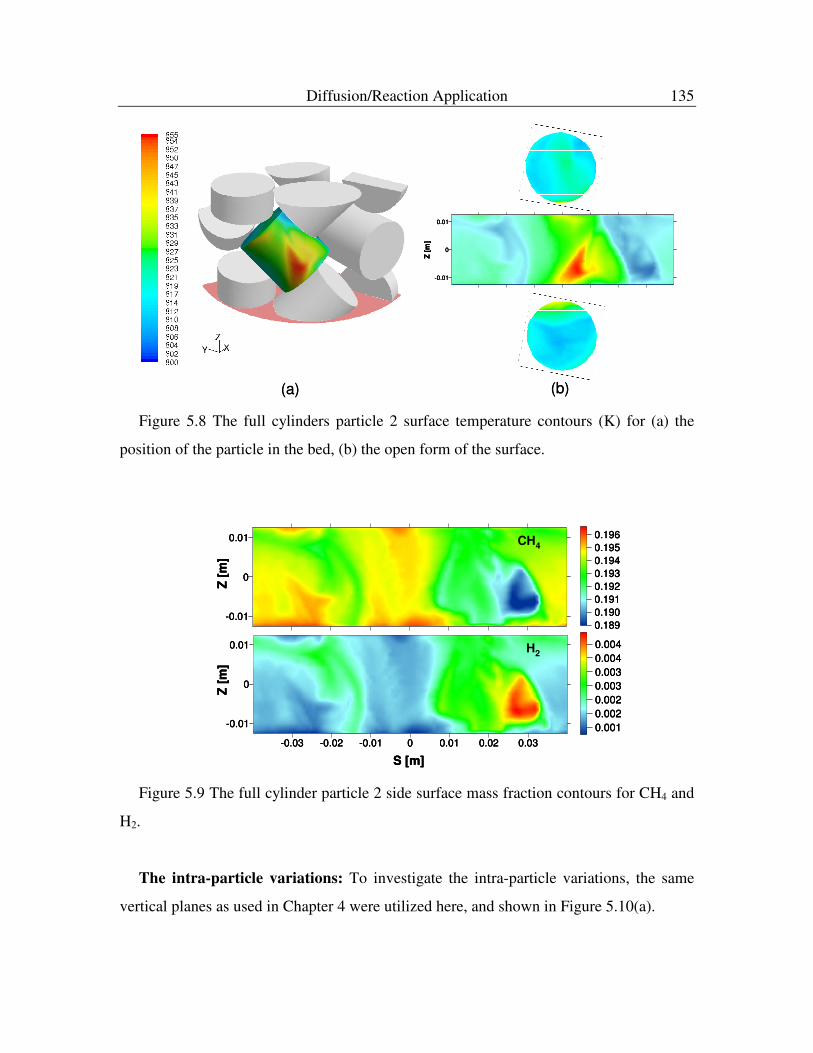