reaction-diffusion equations with applications
TRANSCRIPT
Reaction-Diffusion equations with applications
Christina Kuttler
Sommersemester 2011
Contents
1 Reaction & Diffusion 31.1 Introduction . . . . . . . . . . . . . . . . . . . . . . . . . . . . . . . . . . . . . . . . . . . . 31.2 Examples for typical reactions . . . . . . . . . . . . . . . . . . . . . . . . . . . . . . . . . . 3
1.2.1 Population dynamics . . . . . . . . . . . . . . . . . . . . . . . . . . . . . . . . . . . 31.2.2 Predator-prey . . . . . . . . . . . . . . . . . . . . . . . . . . . . . . . . . . . . . . . 41.2.3 Competition . . . . . . . . . . . . . . . . . . . . . . . . . . . . . . . . . . . . . . . 41.2.4 Symbiosis . . . . . . . . . . . . . . . . . . . . . . . . . . . . . . . . . . . . . . . . . 41.2.5 Chemical reactions . . . . . . . . . . . . . . . . . . . . . . . . . . . . . . . . . . . . 5
1.3 Diffusion equation . . . . . . . . . . . . . . . . . . . . . . . . . . . . . . . . . . . . . . . . 91.3.1 Fick’s law / Conservation of mass . . . . . . . . . . . . . . . . . . . . . . . . . . . 91.3.2 (Weak) Maximum principle . . . . . . . . . . . . . . . . . . . . . . . . . . . . . . . 101.3.3 Uniqueness . . . . . . . . . . . . . . . . . . . . . . . . . . . . . . . . . . . . . . . . 111.3.4 Fundamental solution of the Diffusion equation . . . . . . . . . . . . . . . . . . . . 121.3.5 Including a source . . . . . . . . . . . . . . . . . . . . . . . . . . . . . . . . . . . . 141.3.6 Random motion and the Diffusion equation . . . . . . . . . . . . . . . . . . . . . . 151.3.7 “Time” of Diffusion . . . . . . . . . . . . . . . . . . . . . . . . . . . . . . . . . . . 17
2 Mathematical basics / Overview 192.1 Some necessary basics from ODE theory . . . . . . . . . . . . . . . . . . . . . . . . . . . . 192.2 Boundary conditions . . . . . . . . . . . . . . . . . . . . . . . . . . . . . . . . . . . . . . . 212.3 Separation of Variables . . . . . . . . . . . . . . . . . . . . . . . . . . . . . . . . . . . . . . 222.4 Similarity solutions . . . . . . . . . . . . . . . . . . . . . . . . . . . . . . . . . . . . . . . . 242.5 Blow up . . . . . . . . . . . . . . . . . . . . . . . . . . . . . . . . . . . . . . . . . . . . . . 26
3 Comparison principles 29
4 Existence and uniqueness 314.1 Problem formulation . . . . . . . . . . . . . . . . . . . . . . . . . . . . . . . . . . . . . . . 314.2 Abstract linear problems . . . . . . . . . . . . . . . . . . . . . . . . . . . . . . . . . . . . . 334.3 Abstract semilinear problems . . . . . . . . . . . . . . . . . . . . . . . . . . . . . . . . . . 344.4 Existence and uniqueness for reaction-diffusion problems . . . . . . . . . . . . . . . . . . . 374.5 Global solutions . . . . . . . . . . . . . . . . . . . . . . . . . . . . . . . . . . . . . . . . . . 39
5 Stationary solutions / Stability 405.1 Basics . . . . . . . . . . . . . . . . . . . . . . . . . . . . . . . . . . . . . . . . . . . . . . . 405.2 Example: The spruce budworm model . . . . . . . . . . . . . . . . . . . . . . . . . . . . . 41
6 Reaction-diffusion systems 506.1 What can be expected from Reaction-diffusion systems? . . . . . . . . . . . . . . . . . . . 506.2 Conservative systems . . . . . . . . . . . . . . . . . . . . . . . . . . . . . . . . . . . . . . . 50
6.2.1 Lotka-Volterra system . . . . . . . . . . . . . . . . . . . . . . . . . . . . . . . . . . 506.3 Some more basics for Reaction-diffusion systems . . . . . . . . . . . . . . . . . . . . . . . 52
7 Waves 577.1 Plane waves . . . . . . . . . . . . . . . . . . . . . . . . . . . . . . . . . . . . . . . . . . . . 57
7.1.1 Introduction . . . . . . . . . . . . . . . . . . . . . . . . . . . . . . . . . . . . . . . 577.1.2 Different types of waves . . . . . . . . . . . . . . . . . . . . . . . . . . . . . . . . . 647.1.3 Radially symmetric wave . . . . . . . . . . . . . . . . . . . . . . . . . . . . . . . . 64
1
7.2 Waves in Reaction-Diffusion systems . . . . . . . . . . . . . . . . . . . . . . . . . . . . . . 647.2.1 The spread of rabies . . . . . . . . . . . . . . . . . . . . . . . . . . . . . . . . . . . 657.2.2 Waves of pursuit and evasion in predator-prey systems . . . . . . . . . . . . . . . . 677.2.3 Travelling fronts in the Belousov-Zhabotinskii Reaction . . . . . . . . . . . . . . . 707.2.4 Waves in Excitable Media . . . . . . . . . . . . . . . . . . . . . . . . . . . . . . . . 727.2.5 Travelling Wave Trains in Reaction Diffusion Systems with Oscillatory Kinetics . . 79
7.3 Spiral waves . . . . . . . . . . . . . . . . . . . . . . . . . . . . . . . . . . . . . . . . . . . . 82
8 Pattern formation 878.1 Turing Mechanisms . . . . . . . . . . . . . . . . . . . . . . . . . . . . . . . . . . . . . . . . 878.2 Linear stability analysis for Diffusion-driven instability . . . . . . . . . . . . . . . . . . . . 898.3 Analysis of Pattern Initiation for the Schnakenberg system . . . . . . . . . . . . . . . . . 928.4 Mode Selection . . . . . . . . . . . . . . . . . . . . . . . . . . . . . . . . . . . . . . . . . . 97
8.4.1 White noise . . . . . . . . . . . . . . . . . . . . . . . . . . . . . . . . . . . . . . . . 978.4.2 Travelling wave initiation of patterns . . . . . . . . . . . . . . . . . . . . . . . . . . 988.4.3 Pattern formation in growing domains . . . . . . . . . . . . . . . . . . . . . . . . . 98
8.5 Nonexistence of spatial patterns in reaction diffusion systems . . . . . . . . . . . . . . . . 99
Literature 101
Index 103
2
Chapter 1
Reaction & Diffusion
1.1 Introduction
References: [5]
A reaction-diffusion equation comprises a reaction term and a diffusion term, i.e. the typical form isas follows:
ut = D∆u + f(u)
u = u(x, t) is a state variable and describes density/concentration of a substance, a population ... atposition x ∈ Ω ⊂ R
n at time t (Ω is a open set). ∆ denotes the Laplace operator. So the first term onthe right hand side describes the “diffusion”, including D as diffusion coefficient.The second term, f(u) is a smooth function f : R → R and describes processes with really “change” thepresent u, i.e. something happens to it (birth, death, chemical reaction ...), not just diffuse in the space.It is also possible, that the reaction term depends not only on u, but also on the first derivative of u, i.e.∇u; and/or explicitly on x.Instead of a scalar equation, one can also introduce systems of reaction diffusion equations, which are ofthe form
ut = D∆u + f(x, u,∇u),
where u(x, t) ∈ Rm.
In this lecture, we will deal with such reaction-diffusion equations, from both, an analytical point ofview, but also learn something about the applications of such equations.
1.2 Examples for typical reactions
In this section, we consider typical reactions which may appear as “reaction” terms for the reaction-diffusion equations. When the diffusion (i.e. spatial effects) are ignored, they are ODEs,
u = f(u)
1.2.1 Population dynamics
Often, reaction-diffusion equations are used to describe the spread of populations in space. So, we needsome basics about populations dynamics. Generally, the possible stationary states (where u = 0) andtheir stability are of interest, which correspond to population sizes which don’t change over time.
Exponential growth
f(u) = au
for a = const. (the growth rate).
3
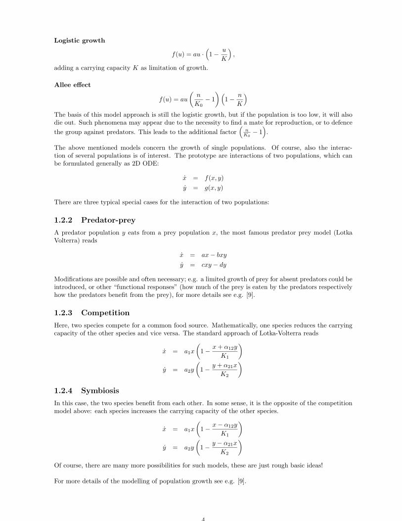
Logistic growth
f(u) = au ·(
1 − u
K
)
,
adding a carrying capacity K as limitation of growth.
Allee effect
f(u) = au
(n
K0− 1
) (
1 − n
K
)
The basis of this model approach is still the logistic growth, but if the population is too low, it will alsodie out. Such phenomena may appear due to the necessity to find a mate for reproduction, or to defence
the group against predators. This leads to the additional factor(
nK0
− 1)
.
The above mentioned models concern the growth of single populations. Of course, also the interac-tion of several populations is of interest. The prototype are interactions of two populations, which canbe formulated generally as 2D ODE:
x = f(x, y)
y = g(x, y)
There are three typical special cases for the interaction of two populations:
1.2.2 Predator-prey
A predator population y eats from a prey population x, the most famous predator prey model (LotkaVolterra) reads
x = ax − bxy
y = cxy − dy
Modifications are possible and often necessary; e.g. a limited growth of prey for absent predators could beintroduced, or other “functional responses” (how much of the prey is eaten by the predators respectivelyhow the predators benefit from the prey), for more details see e.g. [9].
1.2.3 Competition
Here, two species compete for a common food source. Mathematically, one species reduces the carryingcapacity of the other species and vice versa. The standard approach of Lotka-Volterra reads
x = a1x
(
1 − x + α12y
K1
)
y = a2y
(
1 − y + α21x
K2
)
1.2.4 Symbiosis
In this case, the two species benefit from each other. In some sense, it is the opposite of the competitionmodel above: each species increases the carrying capacity of the other species.
x = a1x
(
1 − x − α12y
K1
)
y = a2y
(
1 − y − α21x
K2
)
Of course, there are many more possibilities for such models, these are just rough basic ideas!
For more details of the modelling of population growth see e.g. [9].
4
1.2.5 Chemical reactions
References: [3, 6]
In many applications (bio)chemical reactions are considered, here we just collect a few very basic ideashow to translate such reactions into ODEs.
Law of mass action
We consider a very simple irreversible reaction:
A + Bk−→ C,
k is the so-called reaction rate.Assumption: The change of product in time corresponds to the number of collisions between molecules
A and B, multiplied by the probability that indeed a reaction happens in case of collision (e.g. thereis enough kinetic energy available to initialise the reaction). Let a = [A], b = [B], c = [C] be theconcentrations of A, B and C. The term r1ab∆t approximates the number of collisions in ∆t. For theabove mentioned probability we choose a constant r2, so the change of c in time can be described by
∆c = abk∆t,
where k = r1r2, furthermore (∆t → 0)dc
dt= c(t) = kab,
the so-called Law of mass action. (This is a mathematical model, not a “law”)Remark that reaction rates and concentrations should remain nonnegative!
Reversible reactions
Now we consider a reversible reaction,
A + Bk+
k−
C,
with the reaction rates k+ and k−. Assume that the split-up of C is proportional to c. The correspondingODE system reads:
dc
dt= k+ab − k−c
da
dt= k−c − k+ab
db
dt= k−c − k+ab.
General reaction systems
As a generalisation, we consider now r chemical reactions between s species Ui (with concentrations ui),i = 1, . . . s, which interact simultaneously:
s∑
i=1
lijUikj−→
s∑
i=1
rijUi, j = 1, . . . r.
lij , rij are the so-called stoichiometric coefficients; they describe loss and gain of the number of moleculesUi in reaction j; kj(t) is the corresponding reaction rate (dependency on t might appear due to changeof temperature etc.). The so-called rate function,
gj(t, u) = kj(t)
s∏
n=1
(un)lnj
corresponds to the speed of reaction j and can be used to formulate the ODEs for the ui, as a net resultof all reactions on Ui:
ui =
r∑
j=1
(rij − lij)gj(t, u(t)), i = 1, . . . , s,
5
or in matrix notationu = Sg(t, u(t)),
where u = (u1, . . . , us)T , S = (rij − lij) the stoichiometric matrix of size s × r, g(t, u) = (gj(t, u)) ∈ R
r.
Michaelis-Menten
Literature: Murray [11], a nice short introduction can be found in Wikipedia.
The enzyme kinetics was established by Leonor Michaelis and Maud Menten in 1913. Generally, en-zymes can compensate fluctuating concentrations of substrate, i.e. they adapt their activity and therebytune a steady state. This behaviour is the common one, but of course, there are also exceptions. Inopposite to the kinetics of chemical reactions, in enzyme kinetics there is the phenomenon of saturation.Even for very high concentrations of the substrate, the metabolic rate cannot be increased unlimited,there is a maximum value vmax.Enzymes E, in their function as biocatalytic converter, form together with their substrate S a complexES, from which the reaction to the product performs. Shortly, this can be noted in the following way:
E + Sk1
k−1
ESk2
k−2
EPk3
k−3
E + P.
k1 and k−1 are the rate constants for the association of E and S respectively the dissociation of theenzyme - substrate complex ES. k2 and k−2 are the corresponding constants for the forward reaction tothe product respectively the reverse reaction to the substrate. This reverse reaction does not occur underthe conditions of enzyme kinetics (short after the mixing of the components E and S). Furthermore, theconversion of ES to EP is measured (not the spontaneous release of P ), thus the following simplificationis justified:
E + Sk1
k−1
ESk2→ E + P.
(There is a nice idea, how to understand that kind of kinetics by a descriptive example: S are potatoes,the cook corresponds to the enzyme E - as he has to transform the potatoes into mashed potatoes, theproduct P . Obviously, the cook cannot work infinitely fast with the potatoes, only up to a limit speed;he has to deal with each potato for a certain time - there he forms a complex with the potato. And thereis no chance to get back potatoes from the mushed potatoes :-) ).k2 measures the maximal velocity of reaction under saturated substrate and is also called “turnovernumber”. The Michaelis constant, which is the concentration of substrate, where the metabolic rateassumes half of its maximum, results in
Km =k−1
k1
(in the so-called Michaelis-Menten case, if k2 ≪ k1), or more generally in
Km =k−1 + k2
k1
(called Briggs Haldane situation).
The saturation function of a “Michaelis-Menten enzyme” is described by
v =vmax · [S]
Km + [S],
where v = ˙[P ], the graph looks obviously as follows:
6
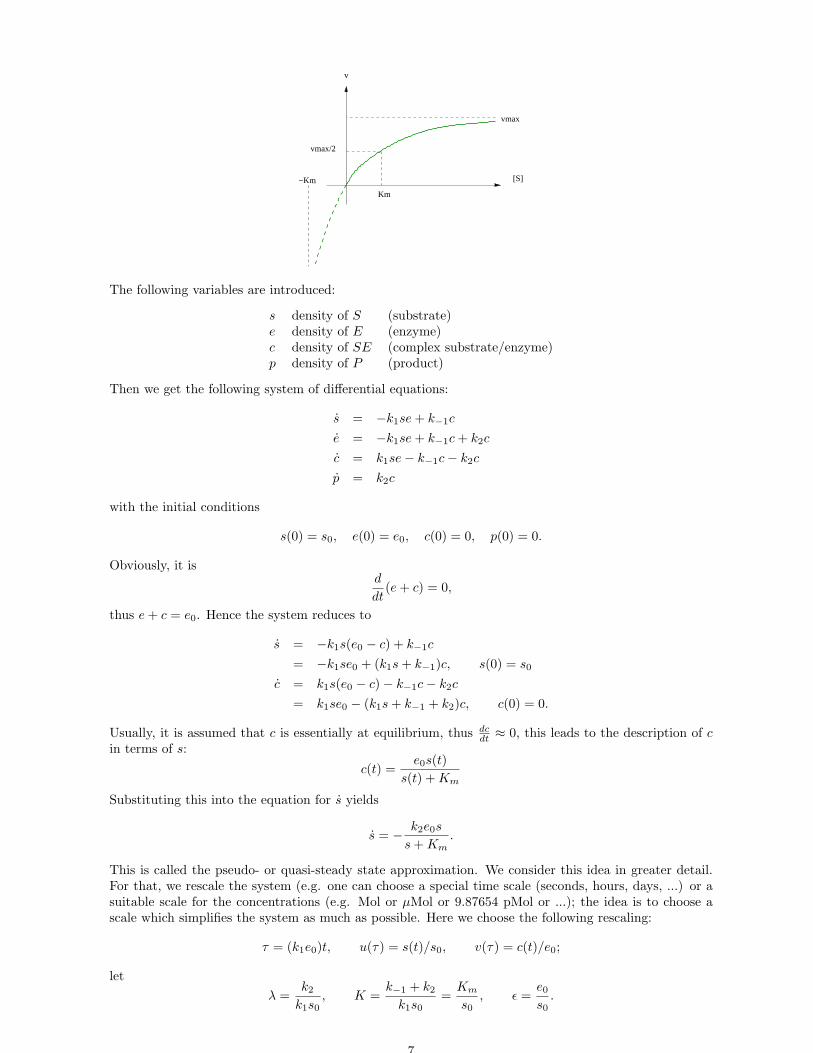
[S]
v
vmax
−Km
vmax/2
Km
The following variables are introduced:
s density of S (substrate)e density of E (enzyme)c density of SE (complex substrate/enzyme)p density of P (product)
Then we get the following system of differential equations:
s = −k1se + k−1c
e = −k1se + k−1c + k2c
c = k1se − k−1c − k2c
p = k2c
with the initial conditions
s(0) = s0, e(0) = e0, c(0) = 0, p(0) = 0.
Obviously, it isd
dt(e + c) = 0,
thus e + c = e0. Hence the system reduces to
s = −k1s(e0 − c) + k−1c
= −k1se0 + (k1s + k−1)c, s(0) = s0
c = k1s(e0 − c) − k−1c − k2c
= k1se0 − (k1s + k−1 + k2)c, c(0) = 0.
Usually, it is assumed that c is essentially at equilibrium, thus dcdt ≈ 0, this leads to the description of c
in terms of s:
c(t) =e0s(t)
s(t) + Km
Substituting this into the equation for s yields
s = − k2e0s
s + Km.
This is called the pseudo- or quasi-steady state approximation. We consider this idea in greater detail.For that, we rescale the system (e.g. one can choose a special time scale (seconds, hours, days, ...) or asuitable scale for the concentrations (e.g. Mol or µMol or 9.87654 pMol or ...); the idea is to choose ascale which simplifies the system as much as possible. Here we choose the following rescaling:
τ = (k1e0)t, u(τ) = s(t)/s0, v(τ) = c(t)/e0;
let
λ =k2
k1s0, K =
k−1 + k2
k1s0=
Km
s0, ǫ =
e0
s0.
7
Hence
d
dτu(τ) =
d
dτ
s(t)
s0=
1
s0
ds(t)
dt
dt
dτ
=1
s0
1
k1e0(−k1se0 + (k1s + k−1)c)
= − s
s0+
1
e0
sc
s0+
k−1
k1
c
s0e0
= −u(τ) + u(τ)v(τ) + (K − λ)v(τ)
= −u + (u + K − λ)v,
in the same way:
εd
dτv(τ) = u − (u + K)v, .
The initial conditions satisfy
u(0) =s(0)
s0= 1 and v(0) =
c(0)
e0= 0.
Usually, there will be much less enzyme than substrate be present in the system, i.e.
ε =e0
s0≪ 1.
This means: In system
u = −u + (u + K − λ)v
εv = u − (u + K)v
there are two processes on two different time scales,
u “normal”
v =1
ε(u − (u + K)v) “very fast” for ε small
The limit ε → 0 corresponds to the“pseudo steady state assumption”
0 = u − (u + K)v ⇔ v =u
u + K.
Insert this into the ODE for u:
u = −u + (u + K − λ)u
u + K= −u + u − λ
u + Ku = − λu
u + K.
For a better understanding of the fast system, we use another time scale:
τ = (k1s0)t ⇔ t =τ
k1s0.
τ is (due to s0 ≫ e0) a kind of “slow motion”, i.e. a time-scale which allows to examine the short timebehaviour of the fast system.Rescaling to the time scale τ yields
du
dτ= ε(−u + (u + K − λ)v)
dv
dτ= u − (u + K)v.
Again, we consider the limit ε → 0:
du
dτ= 0
dv
dτ= u − (u + K)v
8
This means: In the fast system, u doesn’t change at all, so the constant value for u can be inserted intothe ODE for v:
dv
dτ= u − (u + K)v,
Solution for v(0) = v0:
v(τ) = v0e−(u+K)τ +
u
u + K(1 − e−(u+K)τ ),
hence for large times
limτ→∞
v(τ) =u
u + K.
Taken together, this means:
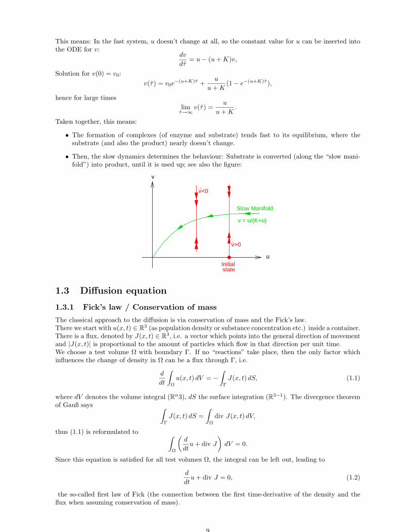
• The formation of complexes (of enzyme and substrate) tends fast to its equilibrium, where thesubstrate (and also the product) nearly doesn’t change.
• Then, the slow dynamics determines the behaviour: Substrate is converted (along the “slow mani-fold”) into product, until it is used up; see also the figure:
Slow Manifold
v = u/(K+u)
v>0.
v<0.
Initialstate
v
u
1.3 Diffusion equation
1.3.1 Fick’s law / Conservation of mass
The classical approach to the diffusion is via conservation of mass and the Fick’s law.There we start with u(x, t) ∈ R
3 (as population density or substance concentration etc.) inside a container.There is a flux, denoted by J(x, t) ∈ R
3, i.e. a vector which points into the general direction of movementand |J(x, t)| is proportional to the amount of particles which flow in that direction per unit time.We choose a test volume Ω with boundary Γ. If no “reactions” take place, then the only factor whichinfluences the change of density in Ω can be a flux through Γ, i.e.
d
dt
∫
Ω
u(x, t) dV = −∫
Γ
J(x, t) dS, (1.1)
where dV denotes the volume integral (Rn3), dS the surface integration (R3−1). The divergence theoremof Gauß says ∫
Γ
J(x, t) dS =
∫
Ω
div J(x, t) dV,
thus (1.1) is reformulated to∫
Ω
(d
dtu + div J
)
dV = 0.
Since this equation is satisfied for all test volumes Ω, the integral can be left out, leading to
d
dtu + div J = 0, (1.2)
the so-called first law of Fick (the connection between the first time-derivative of the density and theflux when assuming conservation of mass).
9
t
x
t=T
t=0
x=0
x=l
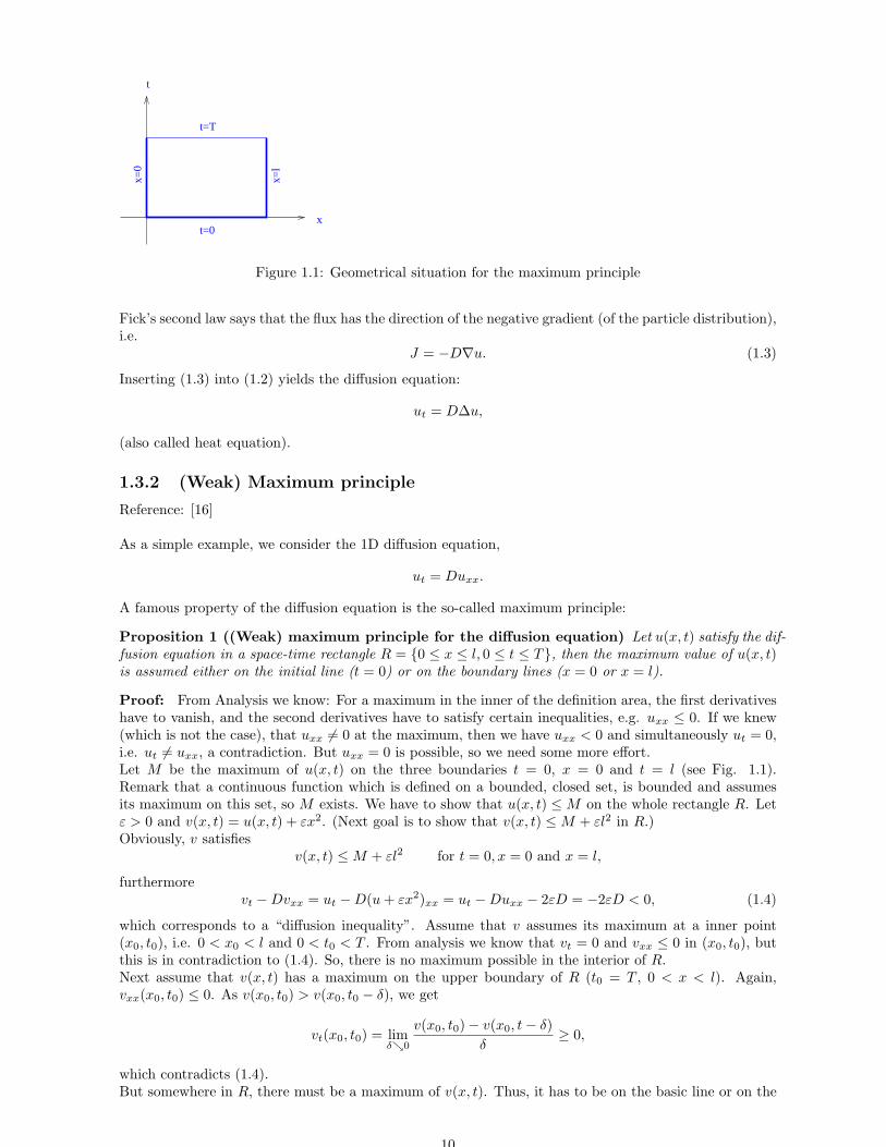
Figure 1.1: Geometrical situation for the maximum principle
Fick’s second law says that the flux has the direction of the negative gradient (of the particle distribution),i.e.
J = −D∇u. (1.3)
Inserting (1.3) into (1.2) yields the diffusion equation:
ut = D∆u,
(also called heat equation).
1.3.2 (Weak) Maximum principle
Reference: [16]
As a simple example, we consider the 1D diffusion equation,
ut = Duxx.
A famous property of the diffusion equation is the so-called maximum principle:
Proposition 1 ((Weak) maximum principle for the diffusion equation) Let u(x, t) satisfy the dif-fusion equation in a space-time rectangle R = 0 ≤ x ≤ l, 0 ≤ t ≤ T, then the maximum value of u(x, t)is assumed either on the initial line (t = 0) or on the boundary lines (x = 0 or x = l).
Proof: From Analysis we know: For a maximum in the inner of the definition area, the first derivativeshave to vanish, and the second derivatives have to satisfy certain inequalities, e.g. uxx ≤ 0. If we knew(which is not the case), that uxx 6= 0 at the maximum, then we have uxx < 0 and simultaneously ut = 0,i.e. ut 6= uxx, a contradiction. But uxx = 0 is possible, so we need some more effort.Let M be the maximum of u(x, t) on the three boundaries t = 0, x = 0 and t = l (see Fig. 1.1).Remark that a continuous function which is defined on a bounded, closed set, is bounded and assumesits maximum on this set, so M exists. We have to show that u(x, t) ≤ M on the whole rectangle R. Letε > 0 and v(x, t) = u(x, t) + εx2. (Next goal is to show that v(x, t) ≤ M + εl2 in R.)Obviously, v satisfies
v(x, t) ≤ M + εl2 for t = 0, x = 0 and x = l,
furthermorevt − Dvxx = ut − D(u + εx2)xx = ut − Duxx − 2εD = −2εD < 0, (1.4)
which corresponds to a “diffusion inequality”. Assume that v assumes its maximum at a inner point(x0, t0), i.e. 0 < x0 < l and 0 < t0 < T . From analysis we know that vt = 0 and vxx ≤ 0 in (x0, t0), butthis is in contradiction to (1.4). So, there is no maximum possible in the interior of R.Next assume that v(x, t) has a maximum on the upper boundary of R (t0 = T , 0 < x < l). Again,vxx(x0, t0) ≤ 0. As v(x0, t0) > v(x0, t0 − δ), we get
vt(x0, t0) = limδց0
v(x0, t0) − v(x0, t − δ)
δ≥ 0,
which contradicts (1.4).But somewhere in R, there must be a maximum of v(x, t). Thus, it has to be on the basic line or on the
10
boundaries of R, and v(x, t) ≤ M + εl2 is valid for whole R.Now it follows immediately that
u(x, t) ≤ M + ε(l2 − x2);
this inequality is valid for all ε > 0, so we get
u(x, t) ≤ M for (x, t) ∈ R.
2
Remark 1 This idea can be extended to a minimum principle and shown by using the maximum principleand applying it on the function −u(x, t).
Remark 2 There is also a strong version of the maximum principle, which says that the maximum isnot assumed in the interior of the rectangle, but exclusively on the initial line or on the boundary lines,except for a constant u. We do not show the proof here.
1.3.3 Uniqueness
An important point is to check uniqueness of solutions for a given problem. In case of the Diffusionequation, an initial condition and boundary conditions (for finite boundaries) have to be prescribed.Here, we consider the so-called Dirichlet problem for the Diffusion equation (including an inhomogeneityf), i.e.
ut − Duxx = f(x, t) for 0 < x < l and t > 0 (1.5)
u(x, 0) = φ(x) (1.6)
u(0, t) = g(t) (1.7)
u(l, t) = h(t). (1.8)
(we consider the theory behind later in detail)
Proposition 2 (Uniqueness of the solution) The Dirichlet problem of the Diffusion equation (1.5)-(1.8) has at most one solution.
Proof:For the proof, we use the so-called “energy integral method”: Assume that there are two solutions u1(x, t),u2(x, t); let w = u1 − u2. According to the definition, w satisfies:
wt − Dwxx = 0 for 0 < x < l and t > 0
w(x, 0) = 0 (initial condition)
w(0, t) = 0 and w(l, t) = 0 (boundary conditions)
Furthermore, we get
0 = 0 · w = (wt − Dwxx) · w =
(1
2w2
)
t
+ (−Dwxw)x + Dw2x.
This equation is integrated:
0 =
∫ l
0
(1
2w2
)
t
dx − [Dwxw]l0︸ ︷︷ ︸
=0 due to bound.cond.
+D
∫ l
0
w2x dx
The t-derivative can be taken out of the integral, thus
d
dt
∫ l
0
1
2(w(x, t))2 dx = −D
∫ l
0
(wx(x, t))2 dx ≤ 0.
This means: The integral∫ l
0w2 dx is monotone decreasing (in t), i.e. in each case we have
0 ≤∫ l
0
(w(x, t))2 dx ≤∫ l
0
(w(x, 0))2︸ ︷︷ ︸
=0 due to init.cond.
dx = 0.
It follows that w(x, t) = 0, thus u1 = u2 for all t ≥ 0.
2
11
1.3.4 Fundamental solution of the Diffusion equation
Reference: [16]
In this subsection, we consider the (1D) diffusion equation on the whole x-axis, i.e. −∞ < x < ∞and t ≥ 0. Obviously, we only need an initial condition, no boundary condition; so we consider theproblem
ut = Duxx for −∞ < x < ∞, t > 0, (1.9)
u(x, 0) = φ(x) (1.10)
Idea: In a first step, we solve the problem for a special function φ(x) and in a second step derive thegeneral solution. For that purpose, we use five so-called “invariance properties” of the Diffusion equation(1.9):
(a) The Translation u(x − y, t) of each solution u(x, t) is also a solution
(b) Each Derivative (ux, ut, uxx ...) of a solution is also a solution
(c) Each Linear combination of solutions of (1.9) is also a solution (due to the linearity of the equation)
(d) Each Integral of a solution is also a solution. Let S(x, t) be a solution of (1.9), then also S(x− y, t)and hence also
v(x, t) =
∫ +∞
−∞S(x − y, t)g(y) dy
for each function g(y) if the integral converges in an adequate manner.
(e) Each Dilation u(√
ax, at) (a > 0) of a solution is also a solution, it can be proved by applying thechain rule: Let v(x, t) = u(
√ax, at), then
vt =∂(at)
∂tut = aut, vx =
∂(√
ax)
∂xux =
√aux, vxx =
√a√
auxx = auxx
We look for a particular solution (denoted by Q(x, t)) of (1.9) satisfying the special initial condition
Q(x, 0) =
1 for x > 00 for x < 0
(1.11)
(Remark that this initial condition doesn’t vary under dilation)Q is determined in three steps:
Step 1: Due to property (e) we know that a dilation x → √ax, t → at leaves Qt = DQxx and the
initial condition (1.11) unchanged, so also Q(x, t) should remain unchanged. This is only possible
if the dependency of Q on x and t is of the combination x/√
t: The dilation leads x√t
to√
ax√at
= x√t.
So we look for Q(x, t) of the following form:
Q(x, t) = g(p) for p =x√4Dt
, (1.12)
the function g still has to be determined. (Remark that√
4D as an additional factor will be usefullater; at the moment it doesn’t play a role).
Step 2: We can formulate an ODE for g, using (1.12) and (1.9):
Qt =dg
dp
∂p
∂t= − x
2t√
4Dtg′(p)
Qx =dg
dp
∂p
∂x=
1√4Dt
g′(p)
Qxx =dQx
dp
∂p
∂x=
1
4Dtg′′(p),
thus
0 = Qt − DQxx = − x
2t√
4Dtg′(p) − 1
4tg′′(p) =
1
t
(
−p
2g′(p) − 1
4g′′(p)
)
,
12
the ODE for g readsg′′ + 2pg′ = 0.
We find g′ = c1 · e−R
2p dp = c1 · e−p2
and
Q(x, t) = g(p) = c1 ·∫
e−p2
dp + c2.
Step 3: For the integral boundaries we choose
Q(x, t) = g(p) = c1
∫ x/√
4Dt
0
e−p2
dp + c2,
which is valid for t > 0. Taking into account the initial condition for Q(x, t), expressed as limitt ց 0, we get:
For x > 0 : 1 = limtց0
Q(x, t) = c1
∫ ∞
0
e−p2
dp + c2 = c1
√π
2+ c2
For x < 0 : 0 = limtց0
Q(x, t) = c1
∫ −∞
0
e−p2
dp + c2 = −c1
√π
2+ c2,
thus c1 = 1√π
, c2 = 12 and
Q(x, t) =1
2+
1√π
∫ x/√
4Dt
0
e−p2
dp for t > 0.
This satisfies all required conditions.
Let S = ∂Q∂x , according to property (b) it is also a solution of (1.9). For an arbitrary (differentiable)
function φ with φ(x) = 0 for large |y|, we define
u(x, t) =
∫ ∞
−∞S(x − y, t)φ(y) dy for t > 0. (1.13)
According to (d), u is also solution of (1.9). Using partial integration yields
u(x, t) =
∫ ∞
−∞
∂Q
∂x(x − y, t)φ(y) dy
= −∫ ∞
−∞
∂
∂y[Q(x − y, t)]φ(y) dy
= −∫ ∞
−∞Q(x − y, t)φ′(y) dy − [Q(x − y, t)φ(y)]
y=+∞y=−∞
︸ ︷︷ ︸
=0
,
hence
u(x, 0) =
∫ ∞
−∞Q(x − y, 0)φ′(y) dy
=
∫ x
−∞φ′(y) dy = φ(x).
So, indeed (1.13) corresponds to the desired solution formula, where
S =∂Q
∂x=
1√4πDt
e−x2/4Dt for t > 0,
i.e.
u(x, t) =1√
4πDt
∫ ∞
−∞e−(x−y)2/4Dtφ(y) dy. (1.14)
S is called e.g. “Fundamental solution” or “Green function”.
In most cases, it is impossible to solve the integral in (1.14) explicitely, but for some special φ(x) itcan be written nicely by using the so-called “error function” (well-known in statistics):
Erf(x) =2√π
∫ x
0
e−p2
dp.
Main properties of the error function are
Erf(0) = 0 and limx→∞
Erf(x) = 1.
13
1.3.5 Including a source
Reference: [16]
Here, we look for the solution of the inhomogeneous Diffusion equation on the real axis,
ut − Duxx = f(x, t) for −∞ < x < ∞, 0 < t < ∞ (1.15)
u(x, 0) = φ(x), (1.16)
φ(x) describes the initial distribution, f(x, t) an additional source / sink term.To show:
u(x, t) =
∫ ∞
−∞S(x − y, t)φ(y) dy +
∫ t
0
∫ ∞
−∞S(x − y, t − s)f(y, s) dy ds (1.17)
is solution of (1.15). How to find this formula? The idea is as follows:For an initial value problem for an ODE
du
dt+ Au(t) = f(t), A constant (1.18)
the variation of constant formula yields a solution of type
u(t) = e−tA +
∫ t
0
e(s−t)Af(s) ds.
Let u(t) ∈ Rn, φ ∈ R
n , A ∈ Rn×n (i.e. (1.18) corresponds to a coupled system of n ODEs). For f(t) = 0
the solution reads u(t) = S(t)φ, where S(t) = e−tA. For f(t) 6= 0 we multiply (1.18) with an “integratingfactor” S(−t) = etA:
d
dt[S(−t)u(t)] = S(−t)
du
dt+ S(−t)Au(t) = S(−t)f(t),
which is integrated from 0 to t:
S(−t)u(t) − S(0)u(0)︸ ︷︷ ︸
φ
=
∫ t
0
S(−s)f(s) ds.
Multiplying with S(t) yields
u(t) = S(t)φ︸ ︷︷ ︸
Solutionofhomog.eq.
+
∫ t
0
S(t − s)f(s) ds.
This formula looks quite similar to the approach in (1.17), there is one term corresponding to the solutionof the homogeneous problem and a second term which takes into account the inhomogeneity. For thesolution of the inhomogeneous Diffusion equation, we use of course S as introduced for (1.14). It is calledalso “source operator”, as it transforms each function φ into a new function, i.e. is an operator.
It remains to show that (1.17) is indeed solution of the PDE and the initial condition (uniqueness ofthe solution is guaranteed). As the term including φ was already examined, we choose here φ = 0 tocheck the second term. Deriving (1.17) yields
∂u
∂t=
∂
∂t
∫ t
0
∫ ∞
−∞S(x − y, t − s)f(y, s) dy ds
=
∫ t
0
∫ ∞
−∞
∂S
∂t(x − y, t − s)f(y, s) dy ds + lim
s→t
∫ ∞
−∞S(x − y, t − s)f(y, s) dy,
(taking into account the singularity of S(x − y, t − s) for t − s = 0. Since S(x − y, t − s) satisfies theDiffusion equation, we find
∂u
∂t=
∫ t
0
∫ ∞
−∞D
∂2S
∂x2(x − y, t − s)f(y, s) dy ds + lim
ε→0
∫ ∞
−∞S(x − y, ε)f(y, t) dy.
= D∂2
∂x2
∫ t
0
∫ ∞
−∞S(x − y, t − s)f(y, s) dy ds + f(x, t)
= D∂2u
∂x2+ f(x, t),
14
which corresponds exactly to the inhomogeneous Diffusion equation.Check of the initial condition: Letting t → 0 in (1.17) yields
limt→0
u(x, t) = φ(x) +
∫ 0
0
. . . = φ(x).
Hence, (1.17) is indeed the desired solution!
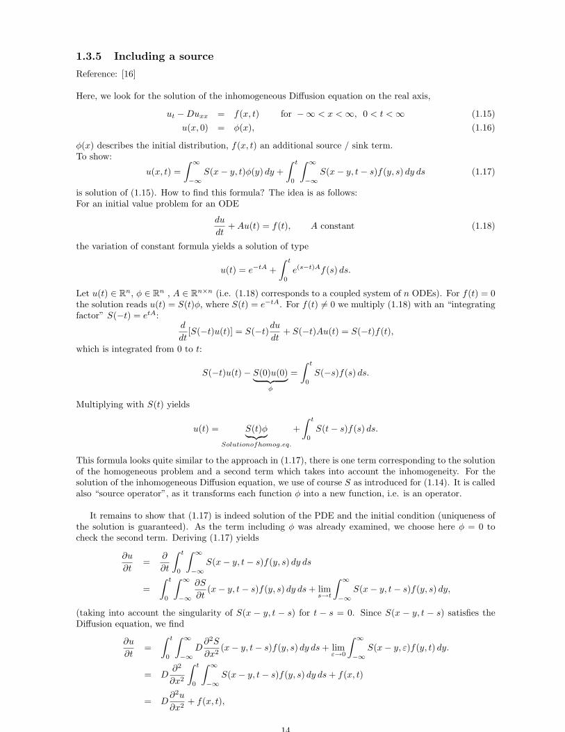
1.3.6 Random motion and the Diffusion equation
Literature: [4, 17]
The Diffusion equation can also be derived from the so-called Random walk / the “Brownian motion”.Here, we consider the following 1D situation (a particle on a 1D grid):
x x+ xx− x∆ ∆
λ rlλ
For the Brownian motion: Per time unit τ , the particles move left or right with an average step length∆x, starting from some x. Which direction they choose, is determined randomly, there is no “connection”between the steps (thus, it is also called “uncorrelated random walk”. Here, we assume equal probabilitiesof moving left (λl) or right (λr), i.e. λl = λr = 1
2 .Let ξk ∈ −∆x,∆x be the shift in the time interval [(k − 1)∆t, k∆t], 1 ≤ k ≤ n and (without loss ofgenerality) x = 0 the starting point, then the complete shift after time t = n · ∆t is xn =
∑nk=1 ξk. If r
steps are made per time unit, then each step of length ∆x needs ∆t = 1r of the time unit and n steps
need n · ∆t = nr of the time unit. The position of the particle, xn at time t = n · ∆t can be interpreted
as a random variable.Let u(x, t) = P (xn = x) at time t = n ·∆t be the probability, that the particle is at position x at time t.It can be given explicitely by the binomial distribution. The probabilities for both directions are equal.x can be displayed as x = m · ∆x, where m ∈ Z (i.e., it is positioned on the grid). Let nl the number ofsteps to the left and nr the number of the steps to the right, performed by the particle. Obviously,
n = nl + nr.
Assuming that the particle is at m · ∆x after n steps, a further condition reads
nr − nl = m.
Taken together, it yields:
2nr = n + m ⇔ nr =n + m
2.
Then we can apply the probability function which belongs to the binomial distribution:
P (xn = m · ∆x) =
(n
nr
)(1
2
)nr
·(
1
2
)n−nr
=
(1
2
)n
·(
nn+m
2
)
=1
2n·(
nn+m
2
)
.
The expected value E(xn) and the variance V (xn) can be gained from the binomial distribution ordetermined directly:
E(xn) = E
(n∑
k=1
ξk
)
=n∑
k=1
E(ξk)
=
n∑
k=1
(−∆x) · P (ξk = −∆x)
︸ ︷︷ ︸
= 12
+(∆x) · P (ξk = ∆x)︸ ︷︷ ︸
= 12
= 0,
15
and
V (xn) = V
(n∑
k=1
ξk
)
=n∑
k=1
V (ξk)
=
n∑
k=1
(−∆x)2 · P (ξk = −∆x)
︸ ︷︷ ︸
= 12
+(∆x)2 · P (ξk = ∆x)︸ ︷︷ ︸
= 12
= (∆x)2 · n = (∆x)2 · n
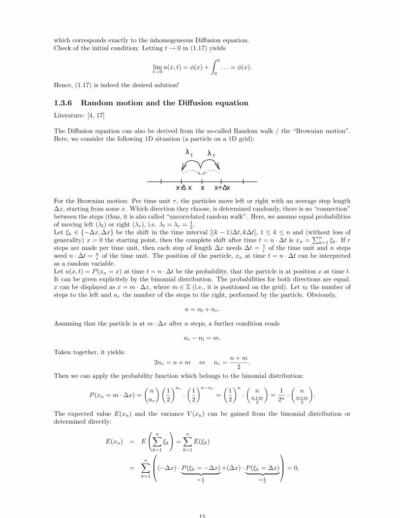
t· t = (∆x)2 · r · t.
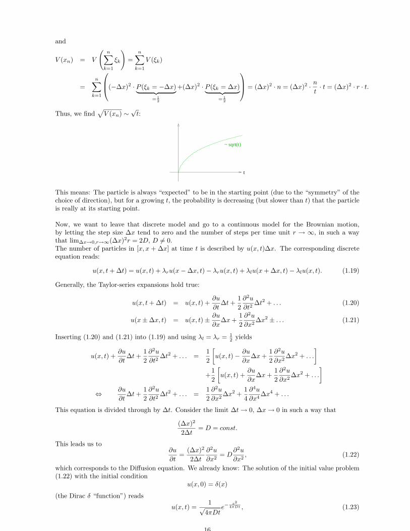
Thus, we find√
V (xn) ∼√
t:
~ sqrt(t)
t
This means: The particle is always “expected” to be in the starting point (due to the “symmetry” of thechoice of direction), but for a growing t, the probability is decreasing (but slower than t) that the particleis really at its starting point.
Now, we want to leave that discrete model and go to a continuous model for the Brownian motion,by letting the step size ∆x tend to zero and the number of steps per time unit r → ∞, in such a waythat lim∆x→0,r→∞(∆x)2r = 2D, D 6= 0.The number of particles in [x, x + ∆x] at time t is described by u(x, t)∆x. The corresponding discreteequation reads:
u(x, t + ∆t) = u(x, t) + λru(x − ∆x, t) − λru(x, t) + λlu(x + ∆x, t) − λlu(x, t). (1.19)
Generally, the Taylor-series expansions hold true:
u(x, t + ∆t) = u(x, t) +∂u
∂t∆t +
1
2
∂2u
∂t2∆t2 + . . . (1.20)
u(x ± ∆x, t) = u(x, t) ± ∂u
∂x∆x +
1
2
∂2u
∂x2∆x2 ± . . . (1.21)
Inserting (1.20) and (1.21) into (1.19) and using λl = λr = 12 yields
u(x, t) +∂u
∂t∆t +
1
2
∂2u
∂t2∆t2 + . . . =
1
2
[
u(x, t) − ∂u
∂x∆x +
1
2
∂2u
∂x2∆x2 + . . .
]
+1
2
[
u(x, t) +∂u
∂x∆x +
1
2
∂2u
∂x2∆x2 + . . .
]
⇔ ∂u
∂t∆t +
1
2
∂2u
∂t2∆t2 + . . . =
1
2
∂2u
∂x2∆x2 +
1
4
∂4u
∂x4∆x4 + . . .
This equation is divided through by ∆t. Consider the limit ∆t → 0, ∆x → 0 in such a way that
(∆x)2
2∆t= D = const.
This leads us to∂u
∂t=
(∆x)2
2∆t
∂2u
∂x2= D
∂2u
∂x2, (1.22)
which corresponds to the Diffusion equation. We already know: The solution of the initial value problem(1.22) with the initial condition
u(x, 0) = δ(x)
(the Dirac δ “function”) reads
u(x, t) =1√
4πDte−
x2
4πDt , (1.23)
16
the fundamental solution.Remark: The assumption that (∆x)2
2∆t tends to a finite limit D 6= 0, if ∆x and ∆t tend to zero, implicates,
that the same limit yields ∆x∆t → ∞. This means: The velocity of a particle which performs Brownian
motion, is infinitely large.This fact also follows from the solution of the initial value problem, (1.23): It is the (Gaussian) normaldistribution, with expected value 0 and the variance 2Dt. Obviously, for all x ∈ R and t > 0, it isu(x, t) > 0, thus, there is a positive probability that the particle is located in a neighbourhood of aposition x, which may be located arbitrarily far away from the origin, as soon as t > 0. Already Einstein,who examined the connection between Brownian motion and diffusion equation first, recognised that thediffusion equation yields a valid model only for large t.
1.3.7 “Time” of Diffusion
Reference: [15]
As it could be “seen” already in the preceding section, in some sense diffusion results in a movementproportional to
√t (i.e. the standard deviation is proportional to
√t). This can be considered also with
a different approach, directly using the PDE.
Theorem 1 Let u be a solution of the 1D diffusion equation
ut = Duxx.
Assume that
C =
∫ +∞
−∞u(x, t) dx
is independent of t (which corresponds to a constant “population”), and u is “small at infinity” whichmeans that
limx→±∞
xu(x, t) = 0 and limx→±∞
x2 ∂u
∂x(x, t) = 0.
Let
σ2(t) =1
C
∫ ∞
−∞x2u(x, t) dx,
thenσ2(t) = 2Dt + σ2(0)
for all t.In the special case of an initial population (i.e. for t = 0) which is concentrated near x = 0 (like a δfunction), then we get σ2(t) ≈ 2Dt.
Remark: σ2(t) is also called the ‘’second moment” (it is finite according to the assumptions), here we useit as a measure, how the density “spreads out”.
Proof: Using the fact that u is solution of the diffusion equation, and applying integration by partstwice yields:
C
D
dσ2
dt=
1
D
∂
∂t
∫ ∞
−∞x2u dx
=1
D
∫ ∞
−∞x2 ∂u
∂tdx
=
∫ ∞
−∞x2 ∂2u
∂x2dx
=
[
x2 ∂u
∂x
]+∞
−∞︸ ︷︷ ︸
=0
−∫ +∞
−∞2x
∂u
∂xdx
= − [2xu]+∞−∞
︸ ︷︷ ︸
=0
+
∫ ∞
−∞2u dx
= 2
∫ ∞
−∞u(x, t) dx = 2C,
17
thusdσ2(t)
dt= 2D.
By integration we get easilyσ2(t) = 2Dt + σ2(0),
as stated in the theorem.Last, we consider the special case that the particles start in a small interval around x = 0, e.g. such thatu(x, 0) = 0 for all |x| > ε. Then we get automatically
∫ ∞
−∞x2u(x, 0) dx =
∫ ε
−ε
x2u(x, 0) dx ≤ ε2
∫ ε
−ε
u(x, 0) dx = ε2C,
thus σ2(0) = ε2 ≈ 0.
2
18
Chapter 2
Mathematical basics / Overview
2.1 Some necessary basics from ODE theory
Reference: [1]
As some methods / approaches for the reaction-diffusion equations (e.g. the travelling wave solutions ortime-independent solutions in 1D for the space) satisfy systems of ODEs, we consider here a few details(without proofs), which may be not so well-known.
For existence and uniqueness, the most prominent theorem is the one of Picard-Lindelof which guar-antees local existence and uniqueness of a solution for u = f(u, t), where fi are Lipschitz continuous.
Considering linear autonomous ODE systems u = Au is “easy” - the unique equilibrium 0 (if A isregular) is stable if Re(λ) ≤ 0 (for all eigenvalues λ of A) with the additional condition that λ has tobe a simple eigenvalue if Re(λ) = 0; it is asymptotically stable (i.e. the solutions really tend to theequilibrium, not only stay “nearby”) if Re(λ) < 0 for all eigenvalues λ. Solutions can be formulated byusing a fundamental system of linearly independent solutions.
For nonlinear ODE systems,u = f(u) = Au + N(u),
where A is a matrix and N(u) = o(u) for u → 0 (which means that |N(U)|/|u| → 0 for |u| → 0).Practically, A corresponds to the Jacobian matrix and N(u) represents the remaining nonlinearity of thesystem. Of course, f(u) is assumed to be sufficiently smooth for these operations.The easiest way is to consider the so-called “linearised stability”, i.e. to consider the linearised systemu = Au and the corresponding eigenvalues for their sign. But only for the case that all eigenvalues λhave real part 6= 0, the stability of the linearised system can be guaranteed to correspond to that of thenonlinear system (Theorem of Hartman-Grobman). So, for some cases other methods are needed. Onewell-known method is to use a so-called Lyapunov function. It is defined as follows:
Definition 1 (Lyapunov function) A function V : Rm → R is called positive definite if
(a) V (0) = 0
(b) V > 0 everywhere else in an open region Ω ⊂ Rm containing 0.
The function V (u) = V (u(t)) for any solution u = u(t) of u = f(u) is a function of t, its derivative is(for a sufficiently smooth V ) defined by
dV
dt= V =
m∑
i=1
∂V
∂uiui =
m∑
i=1
∂V
∂uifi(u)
If V : Rm → R is a function with continuous derivatives, is positive definite and dV
dt ≤ 0 on Ω for anysolution u of u = f(u) is called Lyapunov function for the system u = f(u).
The usefulness of the Lyapunov function is provided by the following two theorems:
Theorem 2 (Lyapunov; Stability) If a Lyapunov function exists for u = f(u) with f(0) = 0, thenthe equilibrium at 0 is stable.
19
It is even possible to proof asymptotic stability by using a Lyapunov function:
Theorem 3 (Lyapunov; Asymptotic stability) If a Lyapunov function exists for u = f(u) withf(0) = 0 and −dV
dt is positive definite, then the equilibrium at 0 is asymptotically stable.
Often, one is interested in the asymptotic behaviour (t → ∞) of solutions. Remark, that many statementsin this context are only possible for 2D systems, not for higher dimensions! So, we consider here a systemlike that:
u = f(u, v) (2.1)
v = g(u, v). (2.2)
For showing the existence of a periodic orbit, a useful theorem is the Theorem of Poincare-Bendixson,which can be formulated as follows:
Theorem 4 (Poincare-Bendixson) If (u, v) remains bounded for t → ∞ and doesn’t tend to an equi-librium, then the trajectory tends to a periodic solution.
Remark: There are different “types” of periodic solutions / systems with periodic solutions. If f andg are sufficiently smooth and the system has at least one periodic solution, then the system either hasa complete family of periodic solutions (corresponding to closed curves G(u, v) = const) in the phaseplane, or just a number of isolated limit cycles. From a biological point or view, only the limit cyclesare relevant, because the first possibility corresponds to a conservative system and includes a “structuralinstability”, i.e. changes the behaviour under small perturbations of the system, so it wouldn’t be ob-servable in reality. So, one is not only interested in the existence / nonexistence of periodic orbits, buteven more in the existence / nonexistence of stable limit cycles, as they can be observed.
For that, invariant sets are useful, they are defined as follows:
Definition 2 (Invariant set) Let Ω be a domain which is enclosed by a simple curve ∂Ω (in the phaseplane). Ω is called invariant set for (2.1),(2.2), if any solution with initial conditions in Ω stays insideΩ for all t > 0.
The easiest way to prove a domain to be an invariant set is the following lemma:
Lemma 1 Let n(u) denote the unit outward normal at u ∈ ∂Ω. If
f(u) · n(u) < 0 ∀n(u) ∈ ∂Ω,
then Ω is an invariant set.
How to use invariant sets to show existence of limit cycles? There, the following theorem helps:
Theorem 5 Let (2.1),(2.2) have an invariant set Ω which includes a unique unstable equilibrium (whichhas to be a focus). Then ω contains a limit cycle.
(This theorem can be shown easily by applying the theorem of Poincare-Bendixson).
The following two theorems deal with the non-existence of limit cycles:
Theorem 6 (Negative criterion of Bendixson-Dulac) If div
(fg
)
= ∂f∂u + ∂g
∂v doesn’t change sign
in an appropriate domain Ω, then no limit cycles can exist in Ω.
(This can be shown by Stokes theorem)For the special case of considering two-component reaction systems the following theorem is useful:
Theorem 7 (Hanusse) A two-component reaction system which contains only bi-molecular reactioncannot show up a limit cycle solution.
For a special type of systems, existence of limit cycles follows.
Definition 3 (Lienard system) A system which can be written as
x + φ(x)x + ψ(x) = 0
and φ(x) and ψ(x) satisfy the following conditions:
20
(i) φ(x) is even, ψ(x) is odd, xψ(x) > 0 for all x 6= 0 and φ(0) < 0
(ii) φ(x) and ψ(x) are continuous; ψ(x) satisfies a Lipschitz condition
(iii) Φ(x) =∫ x
0φ(y) dy → ±∞ for x → ±∞, Φ(x) has a single positive root x = a and is a monotonic
increasing function of x for x ≥ a,
is called “Lienard system”.
Theorem 8 (Lienard system) A Lienard system has a unique stable limit cycle solution.
2.2 Boundary conditions
Reference: [5]
If we consider a reaction diffusion equation on a bounded domain Ω ⊂ Rn, i.e. Ω 6= R
n, then weneed, additional to the initial conditions, well-suited boundary conditions (otherwise, uniqueness cannotbe guaranteed). We consider the equation
ut = ∆u + f(u) for x ∈ Ω ⊂ Rn, t > 0
with the initial conditionsu(x, 0) = u0(x) for x ∈ Ω.
In general, boundary conditions have the form
b(x, t, u,∇u) = 0, for x ∈ ∂Ω, t > 0.
Typical examples are:
Dirichlet boundary conditions:u = b(x, t) for x ∈ ∂Ω, t > 0,
where b is a prescribed function. If b = 0, they are called homogeneous Dirichlet boundary condi-tions.
Neumann boundary conditions:
∇u · n = b(x, t) for x ∈ ∂Ω, t > 0,
where n is the outer normal to Ω at x ∈ ∂Ω. The homogeneous case, b = 0, corresponds to the “noflux condition” - no particles / individuals can leave or enter the domain Ω via the boundaries.
Robin boundary conditions: (also called “mixed boundary conditions”):
α(x, t)u + β(x, t)∇u · n = b(x, t) for x ∈ ∂Ω, t > 0,
notation as above.
Some remarks:
• It is possible to combine different types of boundary conditions on separate parts of the boundary.
• Here, the boundary conditions were introduced as linear conditions in u; it is possible also to havenonlinear boundary conditions (but this makes the analysis possibly more complicated).
• For the existence of solutions of reaction-diffusion equations, the choice of properly posed boundaryconditions and reasonable initial data is essential. We will see that later.
21
2.3 Separation of Variables
References: [15, 16]
Again we start by considering the 1D diffusion equation,
ut = Duxx.
Generally, one tries to determine solution as linear combination of certain easy-to-find solution. Oneoften useful trick is to look for a solution of the special form
u(x, t) = X(x)T (t).
This means: The dependency on variable x and variable t can be separated (an assumption!). Remark:The capitals denote the functions, not the variables. In the following, we use prime for the derivativeswith respect to t and x.Using this approach and insert it into the diffusion equation yields
T ′(t)X(x) = DT (t)X ′′(x) ⇔ DX ′′(x)
X(x)=
T ′(t)
T (t)∀t, x.
Let
λ :=T ′(0)
T (0).
The equation holds for all t and x, thus especially for t = 0, so we get for all x:
DX ′′(x)
X(x)=
T ′(0)
T (0)= λ,
(as the left hand side does not depend on t, and in the same way the right hand side does not depend onx), concluding
DX ′′(x)
X(x)=
T ′(t)
T (t)= λ ∀t, x.
λ is fixed, but so far unknown.This means: X and T satisfy an linear ODE, each (with the same λ, of course). (For simplicity, we takeD = 1 in the following; but no problem to do the same approach for D 6= 0):
X ′′(x) = λX(x)
T ′(t) = λT (t).
The second equation can be easily solved:
T (t) = T (0)eλt,
Also for the first equation, the general solution is easy to determine:
X(x) = ae+√
λx + be−√
λx,
a, b arbitrary constants. If λ < 0, we can rewrite this solution using trigonometric functions:
X(x) = a cos(√−λx) + b sin(
√−λx).
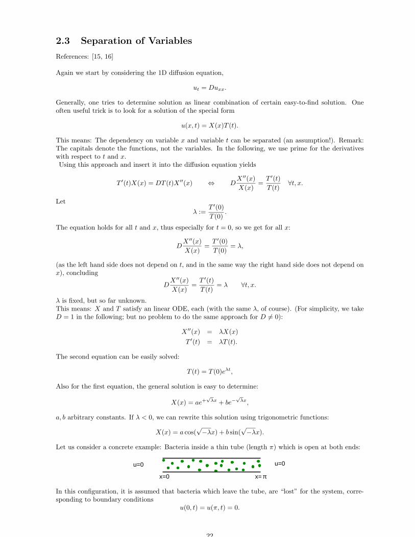
Let us consider a concrete example: Bacteria inside a thin tube (length π) which is open at both ends:
u=0 u=0
x= πx=0
In this configuration, it is assumed that bacteria which leave the tube, are “lost” for the system, corre-sponding to boundary conditions
u(0, t) = u(π, t) = 0.
22
Inside the tube, we assume 1D diffusion, i.e.
ut =∂2u
∂x2
(again we use D = 1 for simplicity).Remark: With these homogeneous Dirichlet boundary conditions, u = 0 is always a solution. We wantto check if further bounded solutions 6= 0 are possible.Concretely, we look for a solution with the separation of variables approach, u(x, t) = X(x)T (t).As introduced above, if a such a solution exists, then a fixed number λ exists with X ′′(x) = λX(x) andT ′(t) = λT (t) for all x, t. Due to T (t) = eλtT (0), it is necessary to have λ ≤ 0 for a bounded solution.λ = 0 can also be excluded, since X ′′(x) = 0 leads to X(x) = ax + b, but the boundary conditions wouldonly allow for a = b = 0 (not a nonzero solution).Let k =
√λ, we know already the general form of the solution of X:
X(x) = a sin kx + b cos kx.
The boundary condition at x = 0 requires
X(0)T (t) = 0 for all t ; X(0) = 0 ; b = 0.
So we have X(x) = a sin kx (and should have a 6= 0). From the boundary condition at x = π it follows:
X(π)T (t) = 0 ∀t ; X(π) = 0 ; sin kπ = 0.
This means: k must be an integer 6= 0.Taken together, if there is a solution of the separated form, then it must look like
u(x, t) = ae−k2t sin kx, k 6= 0 an integer.
Remark: As long as no initial conditions are given, the solution isn’t unique; any linear combination ofsuch solutions yields a solution:
∑
k∈Z
ake−k2t sin kx.
Choosing an initial condition may shrink down the possibilities to one unique solution.As an example, we choose as initial condition:
u(x, 0) = 3 sin 5x − 2 sin 8x.
The presence of two frequencies (5 and 8) in the initial condition hints on that the solution could be ofthe form
u(x, t) = a5e−25t sin 5x + a8e
−64t sin 8x.
As this solution has to satisfy the given initial condition, we can immediately determine the coefficients:
u(x, 0) = a5 sin 5x + a8 sin 8x = 3 sin 5x − 2 sin 8x,
yielding a5 = 3 and a8 = −2, thus
u(x, t) = 3e−25t sin 5x − 2e−64t sin 8x.
Indeed, this is the unique solution for the given problem.
Here we had “easy” initial conditions. If they do not consist of a finite sum∑
k ak sin kx. In themore general case, we need Fourier analysis which allows to write functions on [0, π] as infinite sum∑∞
k=0 ak sin kx, where the idea works in a similar way. We do not consider this in detail here.
In the next example, we consider a reaction-diffusion equation; same situation as above, but the bacteriagrow exponentially:
ut = uxx + αu, u(0, t) = u(π, t) = 0.
The question is, under which conditions for the bacterial growth rate α the population can grow? (Remarkthat in the case above, without growth, the population will die out in the long term run). Easier question:
23
Which α allow for unbounded solutions of the separated form u(x, t) = X(x)T (t)?Again, we start with the separation of variables:
X(x)T ′(t) = X ′′(x)T (t) + αX(x)T (t) ∀x, t,
a (real) λ has to exist such thatT ′(t)
T (t)=
X ′′(x)
X(x)+ α = λ,
yielding now the two coupled equations
T ′(t) = λT (t)
X ′′(x) = (λ − α)X(s),
with the boundary conditions X(0) = X(π) = 0.If λ < 0, then T (t) = eλtT (0) → 0 for t → 0, so the solution will not be unbounded.Thus, we choose λ > 0. Additionally we need λ < α (in order to satisfy the boundary conditions). Thisis shown by contradiction. Assume that λ − α ≥ 0. In this case, a real number µ exists, such thatµ2 = λ − α; X satisfies the equation X ′′ = µ2X.If µ = 0, X becomes linear, X = a + bx; again, the boundary conditions imply a = b = 0, the solutionstays bounded.For µ 6= 0 we get
X = aeµx + be−µx.
The boundary conditions must be satisfied, i.e. a + b = aeµπ + b−µπ = 0, which can be written in matrixform: (
1 1eµπ e−µπ
)(ab
)
=
(00
)
Due to
det
(1 1
eµπ e−µπ
)
= e−µπ − eµπ = e−µπ(1 − e2µπ) 6= 0,
the only solution is a = b = 0, which contradicts X 6= 0. Taken together, λ−α ≥ 0 gives a contradiction,in each case; thus λ < α.Let k be a real number with k2 = α − λ. Hence, we can derive:
X ′′ + k2X = 0 ; X(x) = a sin kx + b cos kx;
the boundary conditions X(0) = X(π) = 0 yield b = 0 and k 6= 0 has to be an integer. Necessarily, α > 1is needed!In general, the solution has the form
aeλt sin kx = ae(α−k2)t sin kx, with a 6= 0, k 6= 0 integer.
Vice versa, every function of this form (or a linear combination of it) is a solution (this has to be checkedseparately).Remark: From a biological point of view, the solution only makes sense if k = 1, otherwise the solutioncontains negative values, which doesn’t make sense for population densities.
2.4 Similarity solutions
Reference: [5]
Idea: By reducing a given problem (in form of a PDE) to a system which contains less independentvariables, it is easier to construct solutions. Such solutions are called similarity solutions or group invari-ant solutions. Typical examples are so-called travelling wave solutions (for autonomous PDEs), we willconsider them later in detail.
Example: We consider an equation of the form
G(ut, u, ux, uxx) = 0,
24
and look for so-called plane travelling wave solutions, which means solutions of the form u = v(z), wherez = x + ct. Introducing this approach into the original equation results in an ODE for v:
G(cvz, v, vz, vzz) = 0
(c is called the wave speed). The solution u = v(z) corresponds to a surface in R3 (i.e. the (x, t, u)-space).
Obviously, the transformationx → x − εc, t → t + ε, u → u (2.3)
doesn’t change this surface (ε a real constant). Mathematically speaking: The solution is invariant underthe group of such transformations. For fixed ε, the transformation (2.3) defines the corresponding groupelement. (Remark: In principle, one should check, if this group satisfies indeed the properties of a group!).Remark also, that such travelling wave solutions only make sense if the underlying PDE does not dependexplicitely on x or t. If this is satisfied, the transformation (2.3) maps solution onto other solutions; but:the existence of such solutions is not trivial!The idea of such transformations can be generalised. We consider PDEs of the form
G(x, t, u, ut, ux, . . .) = 0. (2.4)
Similar to above, the solution u(x, t) corresponds to a surface in the (x, t, u)-space (R3). Now we considera group of transformation for R
3, dependent on one parameter ε ∈ R, of the following form:
x → X(x, t, u, ε)
t → T (x, t, u, ε) (2.5)
u → U(x, t, u, ε)
such thatX = x, T = t, U = u if ε = 0.
If each element of the group of transformations (2.5) maps any solution of PDE (2.4) onto anothersolution of (2.4), then (2.5) is called symmetry group for (2.4).
Example: If we consider the 1D diffusion equation with diffusion coefficient taken to be 1,
ut = uxx,
then the group of transformations
x → εx
t → ε2t (2.6)
u → εαu,
(with α fixed constant) forms a symmetry group for the diffusion equation.How to check this? Let U = εαu, X = εx, T = ε2t, then one get immediately that UT = UXX is true ifu is a solution of the given diffusion equation.
For the more general problem (2.4): Are there any solutions which are invariant under (2.5)? Rememberthat such a solution corresponds to a surface in R
3 which stays unchanged under transformations (2.5).We can formulate this condition by considering a curve
(X(x, t, u, ε), T (x, t, u, ε), U(x, t, u, ε)) : ε ∈ R,
this curve should lie in the surface whenever (x, t, u) does. Fix (x, t, u), then the set
(X(x, t, u, ε), T (x, t, u, ε), U(x, t, u, ε)) : ε ∈ R,
can be interpreted as orbit through (x, t, u).Now we assume that there are two algebraic invariants for transformation (2.5), which means there aretwo functionals of the form
y = y(x, t, u), w = w(x, t, u), (2.7)
which are independent of ε, when the transformation (2.5) is applied - also called “leave unchanged alongorbits”.
25
(In example (2.6), one could choose y = x2/t, w = ut−α/2 as such functionals)We can specify a surface S which is invariant under the group of transformations (2.5) by a relationshipbetween the invariants w and y - this relation corresponds to a surface in R
3. This surface contains thewhole orbits of every point in it! This means that the surface is invariant.Vice versa, for a (given) invariant surface S, the graph of w dependent on y can be obtained; by that allthe orbits which are embedded in S can be obtained, denoted by
w = w(y)
(now y is considered as new independent variable, and the variable w depends on w). How to proceed?(2.7) is assumed to be invertible, i.e. we can can write
u = a(y, w, t)
x = b(y, w, t)
These expressions, and (2.7) are used to calculate the derivatives of u in terms of y, w, t and the ordinaryderivatives wy, wyy.
In our example (2.6) we get:u = t
α2 w and x =
√yt.
The derivatives read
ut =α
2t
α2−1w + t
α2 wyyt
=α
2t
α2−1w + t
α2 wy
−x2
t2
= tα2−1
(α
2w − wyy
)
.
Similarly, the x derivatives can be computed:
ux = tα2 wyyx
uxx = tα2−1(2wy + 4ywyy)
If u is solution of ut = uxx, then we get from the upper reformulations:
tα2−1
(α
2w − wyy
)
= tα2−1(2wy + 4ywyy)
⇔ α
2w − wyy = 2wy + 4ywyy,
i.e. the tα2−1 could be cancelled. Until now, α could be chosen arbitrarily; now we fix it to α = −1,
which yields
4y(wy +w
4)y + 2(wy +
w
4) = 0.
It is sufficient to find a solution for wy + w4 = 0, which reads w = e−
y4 . By that, we get as solution for
ut = uxx:
u = tα2 w = t−
12 e−
x2
4t .
Remark: This corresponds to the already known fundamental solution!
2.5 Blow up
Also from ODEs it is known that solutions may not exist for t → ∞ (global existence) but could tendto ∞ for a finite time t (thus only local existence). Similar things can happen for differential equationsof the reaction-diffusion type: solutions develop a singularity. Here, two different things may happen:
• The singularity may be a point where the dependent variable tends to ∞
• The singularity may be a point where a discontinuity (or a shock) develops
26
If one of these phenomena occurs for finite time (and the solution cannot be continued further), this iscalled a “blow-up”.
We consider the following example:
ut = uxx − u + up for 0 < x < π, t > 0 (2.8)
u(x, 0) = u0(x) ≥ 0 for 0 < x < π (2.9)
u(0, t) = u(π, t) = 0 for t > 0, (2.10)
where p is fixed.Existence and nonnegativity can be shown (we deal with that later). We define (as auxiliary function)
f(t) =
∫ π
0
u(x, t) sin x dx.
So we can multiply the PDE (2.8) by sinx and integrate it from 0 to π:
ft =
∫ π
0
ut sinx dx
=
∫ π
0
uxx sin x dx − f +
∫ π
0
up sin x dx
= −2f +
∫ π
0
up sin x dx.
(Remark: We used integration in parts for this reformulation:
∫ π
0
uxx sin x dx = [ux sinx]π0 −∫ π
0
ux cos x dx
= 0 − [u cos x]π0︸ ︷︷ ︸
u(π,t)−u(0,t)=0, cf. boundary cond.
−∫ π
0
u sinx dx
= −f)
Holder’s inequality says: For p > 1 it holds
∫ b
a
|gh| dx ≤(
∫ b
a
|g|p dx
) 1p
(∫ b
a
|h|p
p−1 dx
)1− 1p
.
Choose g = u · (sin x)1p and h = (sin x)1−
1p (and the integral boundaries a = 0, b = π), then we get
∫ π
0
u sin x dx ≤(∫ π
0
up sin x dx
)1/p
·(∫ π
0
(
(sin x)1−1p
) pp−1
dx
)1− 1p
=
(∫ π
0
up sin x dx
)1/p
·(∫ π
0
sinx dx
)1−1/p
,
which is equivalent to∫ π
0
up sinx dx ≥ fp
2p−1
and
ft = −2f +
∫ π
0
up sinx dx ≥ −2f +fp
2p−1.
Consequently, if we start with an initial value satisfying
f(0) =
∫ π
0
u0(x) sin x, dx > 2p
p−1 ,
then we get
ft(0) ≥ −2f(0) +f(0)p
2p−1= f(0)
(
−2 +f(0)p−1
2p−1
)
︸ ︷︷ ︸
>0
,
27
a monotonously increasing function. We can even write down explicitely the solution of ft = −2f + fp
2p−1 ,for the initial condition f(0) = f0:
f(t) =(
2−p + e2(p−1)t(
f−p+10 − 2−p
))− 1p−1
.
The solution tends to infinity, as
2−p + e2(p−1)t∗(f−p+10 − 2−p) = 0 ⇔ t∗ =
1
2(p − 1)ln
(
2−p
2−p − f−p+10
)
,
i.e. limt→t∗ f(t) → ∞, remark that t∗ < ∞, i.e. finite time.Due to the Cauchy-Schwartz inequality (which can be e.g. formulated by | < x, y > | ≤ ‖x‖ · ‖y‖) we find
f =
∫ π
0
u · sin x dx ≤ ‖u‖L2(0,π) · ‖ sin x‖L2(0,π).
We already know that f → ∞, thus it follows directly that ‖u‖L2(0,π) → ∞, in case of f(0) > 2p/(p−1),i.e. we got the blow-up in finite time.
28
Chapter 3
Comparison principles
Reference: [13]
In this short chapter, we try to compare different solutions of initial-boundary problems in a slightlymore general context than in Chapter 1 (e.g. more general parabolic differential operators).
We consider problems of the following form:
ut = D∆u + f(x, t, u) in GT = Ω × (0, T )
u = 0 on ∂Ω
u(·, 0) = u0 in Ω,
where Ω ⊂ Rn is assumed to be bounded.
We start by stating the strong maximum principle:
Theorem 9 (Strong maximum principle) Let u ∈ C2(GT ), c(x, t) ≥ 0 and D∆u − cu − ut ≥ 0 inGT . Furthermore, let u ≤ M in GT (with M ≥ 0) and u(x0, t0) = M for a (x0, t0) ∈ GT . Then it holds
u(x, t) = M ∀(x, t) ∈ Gt0 .
(This means: If the maximum is assumed in the inner of the definition area, then the solution is constant,at least until time t0).From this theorem, a weak maximum principle can be derived which doesn’t need a nonnegative c.
Theorem 10 (Weak maximum principle) Let u ∈ C2(GT )∩C(GT ), c(x, t) ≥ cmin and D∆u− cu−ut ≥ 0 in GT . Furthermore, let u ≤ 0 in Ω × 0 (i.e. for the initial condition) and in ∂Ω × (0, T ) (i.e.on the boundaries). Then it holds
u(x, t) ≤ 0 ∀(x, t) ∈ GT .
Proof: We introduce an auxiliary function, v(x, t) = ecmintu(x, t). This function satisfies
D∆v − (c − cmin)v − vt = ecmintD∆u − (c − cmin)ecmintu − cmin ecmintu(x, t)︸ ︷︷ ︸
v
−ecmintut
= ecmint(D∆u − cu − ut) ≥ 0;
obviously c− cmin ≥ 0 according to the definition of cmin. Then we know from Theorem 9: v can assumea positive maximum in GT only if it is assumed also for t = 0 or for x ∈ ∂Ω. But v ≤ 0 in Ω × 0 andin ∂Ω × (0, T ), thus we get v ≤ 0 in GT ; u ≤ 0 in GT .
2
The next theorem allows for comparison of two solutions in GT :
Theorem 11 (Comparison principle) Let u, v ∈ C2(GT )C(GT ) and
D∆u + f(x, t, u) − ut ≤ D∆v + f(x, t, v) − vt in GT ,
furthermore u ≥ v in Ω × 0 and in ∂Ω × (0, T ). Then it holds
u(x, t) ≥ v(x, t) ∀(x, t) ∈ GT .
29
Proof: Let w = v − u. From the mean value theorem (differential form) we know:
f(x, t, v) − f(x, t, u) =∂f
∂u(x, t, ξ) (v − u)
︸ ︷︷ ︸
=w
for a ξ satisfyingu(x, t) ≤ ξ(x, t) ≤ v(x, t).
This yields:
D∆w + c(x, t)w − wt = D∆v − D∆u + f(x, t, v) − f(x, t, u) − vt + ut ≥ 0
due to the assumption, where c(x, t) = ∂f∂u (x, t, ξ(x, t)). Now we can apply the weak maximum principle
on w which results inw ≤ 0 in GT ; u ≥ v in GT .
2
From that theorem, we get immediately a statement about uniqueness for initial boundary conditions:
Corollary 1 Let u1, u2 ∈ C2(GT ) ∩ C(GT ) solutions of the reaction diffusion equation
ut = D∆u + f(x, t, u),
with u1 = u2 on Ω × 0 and on ∂Ω × (0, t). Then it follows that
u1 = u2 in GT .
For the application of the comparison principle, we consider an example; the diffusion equation with Alleeeffect as reaction term:
ut = ∆u + u(1 − u)(u − a)︸ ︷︷ ︸
f(u)
for x ∈ Ω, t > 0, (3.1)
where 0 < a < 1, a const., Ω a bounded set in Rn; the homogeneous Dirichlet boundary condition
u = 0 on ∂Ω
and bounded initial data0 ≤ u(x, 0) ≤ 1 ∀x ∈ Ω.
(Remark that the homogeneous Dirichlet condition means: no population at the boundary; possibly allindividuals which arrive at the boundary are somehow “killed”)As a simple possibility, we choose a so-called sub-solution u(x, t) and a super-solution u(x, t):
u = 0
u = 1
(both are independent of x), obviously both, u and u are solutions of (3.1), so we have
D∆u + f(u) − ut ≥ D∆u + f(u) − ut
D∆u + f(u) − ut ≥ D∆u + f(u) − ut
and
u ≥ u in Ω × 0 and ∂Ω × (0, T )
u ≥ u in Ω × 0 and ∂Ω × (0, T ),
i.e. if a solution of (3.1) exists, then the comparison principle yields 0 ≤ u(x, t) ≤ 1.We can even say more: If 0 ≤ u(x, 0) < a ∀x ∈ Ω, we can compare u(x, t) with s(t) (independent of x),where
st = s(1 − s)(s − a)
with initial value s(0) = maxx∈Ω u(x, 0). Obviously s satisfies (3.1), the required comparison conditions,and it is s(t) → 0 for t → ∞, if s(0) < a, so the comparison principle yields u → 0 for t → ∞ (fasterthan s(t)).
30

Chapter 4
Existence and uniqueness
Reference: [13]
We consider the simple example (with homogeneous Neumann boundary conditions)
ut = ∆u + f(u, t) in Ω × (0,∞) (4.1)
∂u
∂ν= 0 for x ∈ ∂Ω.
Obviously, each solution of the ODE v′ = f(v, t) is also solution (spatially independent) of equation(4.1). For ODEs, we know already that some conditions for f are necessary to guarantee existence anduniqueness of solutions. So, also for reaction-diffusion equations, conditions on f can be expected. Localexistence (for small time intervals) is influenced by smoothness of f , whereas global existence is moreinfluenced by the growth behaviour of f as function of u.
4.1 Problem formulation
Here, we consider initial boundary value problems for systems of reaction-diffusion equations,
ut = D∆u + f(t, x, u,∇u), for x ∈ Ω, t > 0 (4.2)
u(x, t) = 0 for x ∈ ∂Ω, t > 0, (4.3)
u(x, t) = u0(x) for x ∈ Ω, (4.4)
where Ω ⊂ Rn is a bounded domain with smooth boundary. Let u(x, t) ∈ R
m and all diffusion coefficientsbe positive: D = diag(D1, . . . ,Dm), Di > 0 for i = 1, . . . m. We start with f = 0.From the theory of linear parabolic equations (generalisation for the diffusion equation) it is known: Thisproblem has a unique solution for each u0 ∈ L2(Ω) (to be correct, one should write L2(Ω)m, but the mis left out, for simplification) which can formally be written as
u(t) = eLtu0,
the operator L is given byD(L) = H2(Ω) ∩ H1
0 (Ω), Lu := D∆u.
Remark: Often, PDEs cannot be solved in the “classical function spaces”, then so-called Sobolev spacesare needed and the concept of weak derivatives. Here, they are based on L2(Ω). Two functions areidentified if u(x) = v(x) for x ∈ Ω except for a nullset. Via the scalar product
(u, v)0 := (u, v)L2 =
∫
Ω
u(x)v(x) dx
L2(Ω) becomes a Hilbert space with the norm
‖u‖0 =√
(u, u)0.
31
The weak derivative is defined as follows: u ∈ L2(Ω) has a weak derivative v = ∂αu in L2(Ω), if v ∈ L2(Ω)and
(φ, v)0 = (−1)|α|(∂αφ, u)0 for all φ ∈ C∞0 (Ω).
α = (α1, . . . , αn) ∈ Nn0 is a so-called multiindex with
|α| = α1 + . . . + αn,
e.g. it can be used as xα = xα1
1 · . . . · xαnn and ∂αφ =
(∂α1
∂xα11
. . . ∂αn
∂xα2n
)
u.
The idea behind is: one multiplies the weak derivative by φ and integrates the product by parts. Theweak derivative is a generalisation of the classical derivative. If a function u is classically differentiableon a bounded domain Ω ⊂ R
n, then the classical derivative corresponds to the weak derivative.C∞
0 (Ω) denotes the subspace of C∞(Ω) which assume only in a compact subset of Ω values 6= 0.If function is differentiable in the classical sense, then the weak derivative also exists and both derivativescorrespond to each other.Definition: Hm(Ω) (for m ≥ 0 integer) denotes the set of all functions u ∈ L2(Ω) which have weakderivatives ∂αu for all |α| ≤ m. A scalarproduct in Hm(Ω) is defined by
(u, v)m :=∑
|α|≤m
(∂αu, ∂αv)0,
with the corresponding norm
‖u‖m :=√
(u, u)m =
√∑
|α|≤m
‖∂αu‖2L2(/Ω).
(The letter H was chosen in honour of David Hilbert).A proposition say: Let Ω ⊂ R
n open with piecewise smooth boundary, m ≥ 0. Then C∞(Ω) ∩ Hm(Ω) isdense in Hm(Ω). So, Hm(Ω) is the “completion“ of C∞(Ω) ∩ Hm(Ω) for bounded Ω. This idea can begeneralised for functions with zero boundary conditions C∞
0 (Ω) and is denoted by Hm0 (Ω)
Some more functional analysis, without considering all details, just to get an overview:As the operator L has a compact symmetric inverse, there is a complete (in L2(Ω)) orthonormal systemϕk, k = 1, 2, . . . of eigenfunctions. Furthermore,
Lu =∞∑
k=1
λk < u,ϕk > ϕk, for u ∈ D(L),
where 0 > λ1 > λ2 > . . . are the eigenvalues of L (limk→∞ λk = −∞) and < ·, · > denotes the innerproduct (scalarproduct) in L2(Ω).For real functions g (with a definition area which comprises the spectrum of L), we define the operatorg(L) by
g(L)u =
∞∑
k=1
g(λk) < u,ϕk > ϕk, for u ∈ D(g(L)).
The definition area of g(L) reads
D(g(L)) =
u ∈ L2(Ω) :
∞∑
k=1
g(λk)2 < u,ϕk >2< ∞
(by using the so-called Parseval equality). For bounded functions, it is D(g(L)) = L2(Ω).The solution of the linear homogeneous initial value problem can be written as
u(t) = eLtu0 =
∞∑
k=1
eλkt < u0, ϕk > ϕk, for t ≥ 0.
It is u ∈ C([0,∞), L2(Ω))∩C1(0,∞), L2(Ω)), u(t) ∈ D(L) for t > 0 and du/dt(t) = Lu(t) for t > 0. Thefamily eLt, t ≥ 0 of bounded linear operators can be interpreted as (strongly continuous) semigroupwith generator L, as the corresponding properties are satisfied:
• eL(t+s) = eLteLs, eL0 = I (semigroup)
• limt→0 eLtu = u (continuity)
• limh→0eLh−I
h u = Lu for u ∈ D(L).
32
4.2 Abstract linear problems
Next, we consider initial value problems for so-called abstract ordinary differential equations in a Hilbertspace (denoted by H), which can be written as
du
dt= Lu(t) + f(t), t ∈ (0, T ], (4.5)
u(0) = u0.
We assume that the linear operator L : D(L) ⊂ H → H is defined by
Lu =∞∑
k=1
λk < u,ϕk > ϕk, u ∈ D(L)
as above, and ϕk, k = 1, 2, . . . forms a complete orthonormal system in H and it holds that
0 > λ1 > λ2 > . . . , limk→∞
λk = −∞.
With these assumptions, one gets the following lemma:
Lemma 2 The definition domain D(L) is dense in H, and L is a closed operator.
The proof is left out here; “closed linear operators” are an important class of linear operators on Banachspaces (something more general than bounded operators, but e.g. the spectrum can be defined).
In the following, the inhomogeneity f is assumed to satisfy f ∈ C([0, T ],H).A classical solution is defined as follows:
Definition 4 A classical solution u ∈ C([0, T ],H) ∩ C1((0, T ],H) of problem (4.5) must satisfy u(t) ∈D(L) for t ∈ (0, T ], and be solution of (4.5).
(Remark: u(t) ∈ D(L) means: u ∈ L2(Ω) and∑∞
k=1 λ2k < u,ϕk >2< ∞.
One idea to find such a solution is the variation of constant formula:
u(t) = eLtu0 +
∫ t
0
eL(t−s)f(s) ds (4.6)
This function is called “mild solution”, which is in some sense a generalisation of the concept of a solution.
Proposition 3 There is at most one classical solution of (4.5). If it exists, then it is equal to the mildsolution (4.6).
Proof: Assume, that a classical solution u exists. Let g(s) = eL(t−s)u(s). By deriving this g, we get:
dg
ds= −LeL(t−s)u(s) + eL(t−s)(Lu(s) + f(s))
= eL(t−s)f(s).
This equation can be integrated (for s from 0 to t) and yields
e0u(t) − eLtu(0) = g(t) − g(0) =
∫ t
0
dg
dsds =
∫ t
0
eL(t−s)f(s) ds
⇔ u(t) = eLtu0 +
∫ t
0
eL(t−s)f(s) ds,
which corresponds exactly to (4.6).
2
We shortly mention (without proof) an auxiliary lemma which helps to show the existence of the classicalsolution:
33
Lemma 3 For each δ > 0 there exists a c > 0 such that
‖LeLt‖ ≤ ct−1e(λ1+δ)t, for t > 0.
We need to know how a locally Holder continuous function is defined:
Definition 5 A function f is called locally Holder continuous, if for all t ∈ (0, T ] there exist δ, c, α > 0such that
‖f(t1) − f(t2)‖ ≤ c|t1 − t2|α, for t1, t2 ∈ (t − δ, t + δ),
where ‖u‖ =√
< u, u > is the norm which is induced by the scalar product in H.
Proposition 4 (Existence classical solution) Let f be locally Holder continuous in (0, T ]. Thenproblem (4.5) possesses a classical solution.
Rough idea for the proof of this proposition: It is sufficient to show that
v(t) =
∫ t
0
eL(t−s)f(s) ds = v1(t) + v2(t)
=
∫ t
0
eL(t−s)[f(s) − f(t)] ds +
∫ t
0
eL(t−s)f(t) ds
is a classical solution of the problem with homogeneous initial condition; for that v(t) ∈ D(L) for t > 0is needed, and Lv(t) is continuous for t > 0. For that, Lemma 3 is useful.
4.3 Abstract semilinear problems
Here, we generalise the approaches to nonlinear problems of the following form:
du
dt(t) = Lu(t) + f(t, u(t)), for t > 0, (4.7)
u(0) = u0.
For the operator L we take the same assumptions as in the section above.We will need powers (−L)α for 0 ≤ α ≤ 1. Introduce as new notations
Hα := D((−L)α) and ‖u‖α := ‖(−L)αu‖
Also (−L)α (as L) is a closed operator; thus Hα is a Banach space with respect to the so-called Graphnorm ‖u‖ + ‖u‖α. We find:
‖u‖2 =
∞∑
k=1
< u,ϕk >2
≤ (−λ1)−2α
∞∑
k=1
(−λk)2α < u,ϕk >2
= (−λ1)−2α‖u‖2
α
(the first equality is due to Parseval’s equation; due to 0 > λ1 > λ2 > . . . , limk→∞ λk = −∞ it is(−λk)2α/(−λ1)
2α ≥ 1)Hence, it follows that the graph norm is equivalent to the norm ‖u‖α and we can use this as norm onHα.The next lemma provides auxiliary estimates:
Lemma 4 Let 0 ≤ α ≤ 1, then it holds
‖(−L)αeLt‖ ≤ cαt−α, for t > 0 (4.8)
‖eLtu − u‖ ≤ tα‖(−L)αu‖, for t ≥ 0, u ∈ Hα. (4.9)
34
Proof: For all x ∈ R it is ex ≤ ex, choosing x = −λkt/α, we get
−eλkt/α ≤ e−λkt
α
⇔ −eλkt
αλkt
αe ≤ 1
⇔ −λkeλkt
α ≤(
αe
)1t
⇔ (−λk)αeλkt ≤(α
e
)α
t−α.
Generally (definition of the operator),
(−L)αeLtu =
∞∑
k=1
(−λk)αeλkt < u,ϕk > ϕk,
by using the Parseval equation we get:
‖(−L)αeLtu‖2 =
∞∑
k=1
|(−λk)αeλkt < u,ϕk > ϕk|
≤ (λk)αe1λkt
︸ ︷︷ ︸
≤(αe )
αt−α
∑
k=1
∞| < u,ϕk > ϕk|︸ ︷︷ ︸
‖u‖2
(λk is chosen to yield the maximum of this term), taken together
‖(−L)αeLt‖ ≤ cαt−α.
Analogously, one can show the second inequality.
2
In the next step, we formulate a condition/assumption for the nonlinearity f in (4.7) which should besufficient for the unique solubility. Let 0 ≤ α < 1 and U an open subset of Hα.
Assumption (NONLIN): For f : [0, T ) × U → H let exist for each u0 ∈ U a neighbourhood V ⊂ U ofu0, and t ≤ T , L ≥ 0 and 0 < ϑ ≤ 1, such that
‖f(t1, u1) − f(t2, u2)‖ ≤ L(|t1 − t2|ϑ + ‖u1 − u2‖α
)for t1, t2 < t, u1, u2 ∈ V.
Theorem 12 Let assumption (NONLIN) hold. Then for each u0 ∈ U a t0 > 0 exists, such that (4.7)has a unique classical solution u ∈ C([0, t0),H) ∩ C1((0, t0),H).
Proof: We write the neighbourhood from (NONLIN) in the following way:
V = u ∈ Hα : ‖u − u0‖α ≤ δ
. Furthermore, letB = max
0≤t≤t‖f(t, u0)‖.
This maximum exists as f is continuous in [0, t]. Now we choose t0 > 0 such that both,
‖eLt(−L)αu0 − (−L)αu0‖ <δ
2, for 0 ≤ t < t0
and
t0 < min
t,
(δ(1 − α)
2cα(B + δL)
) 11−α
are satisfied (cα is the constant from the lemma above). Let
χ = C([0, t0],H) and ‖x‖χ = max0≤t≤t0
‖x(t)‖ for x ∈ χ.
35
We define a nonlinear operator F : χ → χ by
F (x)(t) = eLt(−L)αu0 +
∫ t
0
(−L)αeL(t−s)f(s, (−L)−αx(s))ds.
Obviously it is F (x)(0) = (−L)αu0 for all x ∈ χ. We define a set S:
S = x ∈ χ : x(0) = (−L)αu0, ‖x − (−L)αu0‖χ ≤ δ.
Remark: For x ∈ S and for t ∈ [0, t0] it is (−L)−αx(t) ∈ V .Let x ∈ S, then we get (using the lemma above and the remark; remember also x ∈ S):
‖F (x)(t) − (−L)αu0‖ ≤ ‖eLt(−L)αu0 − (−L)αu0‖
+
∥∥∥∥
∫ t
0
(−L)αeL(t−s)[f(s, (−L)−αx(s)) − f(s, u0)] ds
∥∥∥∥
+
∥∥∥∥
∫ t
0
(−L)αeL(t−s)f(s, u0) ds
∥∥∥∥
≤ δ
2+
∫ t
0
cα(t − s)−αLδ ds +
∫ t
0
cα(t − s)−αB ds
=δ
2+ cα(Lδ + B)
t1−α
1 − α≤ δ.
This means: F maps S onto itself. Furthermore, we get for x1, x2 ∈ S:
‖F (x1)(t) − F (x2)(t)‖ ≤∫ t
0
∣∣∣(−L)αeL(t−s)[f(s, (−L)−αx1(s)) − f(s, (−L)−αx2(s))]
∥∥∥ ds
≤∫ t
0
cα(t − s)−αL‖x1(s) − x2(s)‖ ds
≤ cαLt1−α
1 − α|x1 − x2|χ
≤ 1
2‖x1 − x2‖χ.
just by using the assumption for f and the definition of ‖u‖α. We have shown now: F : S → S is acontraction; thus Banach’s fixed point theorem yields existence (and uniqueness) of a fixed point x ∈ Sof F .We take this fixed point x (which satisfies F (x)(t) = x(t)) and consider (−L)−αx:
(−L)−αx = (−L)−α
[
eLt(−L)αu0 +
∫ t
0
(−L)αeL(t−s)f(s, (−L)−αx(s)) ds
]
= eLtu0 +
∫ t
0
eL(t−s)f(s, (−L)−αx(s)) ds,
i.e. (−L)−αx is by definition a mild solution of (4.7).Still to show: it is also a classical solution. Du to x ∈ χ, the map t 7→ f(t, (−L)−αx(t)) is continuous in[0, t0]. To show: This map is also locally Holder continuous in (0, t0].Let N = ‖f(·, (−L)−αx(·))‖χ. For 0 < β < 1 − α and 0 < h < 1 the application of Lemma 4 (bothinequalities) yields:
‖(eLh − I)(−L)αeLt‖ ≤ hβ‖(−L)β(−L)αeLt‖= hβ‖(−L)α+βeLt‖≤ hβcα+βt−(α+β). (4.10)
36

For 0 < t < t + h ≤ t0 we get
‖x(t + h) − x(t)‖ = ‖F (x)(t + h) − F (x)(t)‖≤ ‖eL(t+h)(−L)αu0 − eLt(−L)αu0‖
+‖∫ t+h
0
(−L)αeL(t+h−s)f(s, (−L)−αx(s)) ds
−∫ t
0
(−L)αeL(t−s)f(s, (−L)−αx(s)) ds‖
≤ ‖eL(t+h)(−L)αu0 − eLt(−L)αu0‖
+
∫ t
0
‖(−L)α(eLh − I)eL(t−s)f(s, (−L)−αx(s))‖ ds
+
∫ t+h
t
‖(−L)αeL(t+h−s)f(s, (−L)−αx(s))‖ ds
=: I1 + I2 + I3.
Using (4.10) allows us to find estimates for the three terms I1, I2, I3:
I1 ≤ cα+βhβt−(α+β)‖u0‖ ≤ c1(t)hβ
I2 ≤ cα+βhβN
∫ t
0
(t − s)−α+β) ds ≤ c2hβ
I3 ≤ cαN
∫ t+h
t
(t + h − s)−α ds = cαNh1−α
1 − α< c3h
β
due to β < 1 − α and h < 1.So, the map t 7→ x(t) is locally Holder continuous in (0, t0]. Furthermore we get (due to assumption(NONLIN)):
‖f(s, (−L)−αx(s)) − f(t, (−L)−αx(t)‖ ≤ L(|s − t|ϑ + ‖x(s) − x(t)‖)≤ L(|s − t|ϑ + c|s − t|β),
which means that also the map t 7→ f(t, (−L)−αx(t)) is locally Holder continuous in (0, t0].From Prop. 4 we know that the linear problem
du
dt(t) = Lu(t) + f(t, (−L)−αx(t)), for t > 0 (4.11)
u(0) = u0
has a unique classical solution u, which is given by
u(t) = eLtu0 +
∫ t
0
eL(t−s)f(s, (−L)−αx(s)) ds.
Now we can apply (−L)α on this equation and find that
(−L)αu(t) = F (x)(t) = x(t) ⇔ u(t) = (−L)−αx(t),
hence u is a classical solution of (4.7).Uniqueness of x and uniqueness of the solution of (4.11) provide uniqueness of the desired classicalsolution.
2
4.4 Existence and uniqueness for reaction-diffusion problems
In this section, we consider a result concerning existence and uniqueness for the problem (4.2-4.4). Wedo not go into deep details, trying to avoid too much knowledge about Sobolev spaces / embedding /PDE theory, but the basic ideas.
The Sobolev spaces (on the domain Ω ⊂ Rn) are defined as follows:
37
Definition 6 For 1 ≤ p < ∞ and k ∈ N
W k,p(Ω) = u ∈ Lp(Ω)|∂αu ∈ Lp(Ω) ∀ |α| ≤ k.
is called Sobolev space.
The corresponding norm in W k,p(Ω) is denoted by ‖ · ‖k,p =(∑
|α|≤k ‖∂αu‖pLp
) 1p
, then W k,p(Ω) is a
Banach space.
We need to know what an ”embedding” means roughly:
Definition 7 Let (X, ‖ · ‖X) and (Y, ‖ · ‖Y ) be Banach spaces.
1. If a linear injective map j : X → Y exists, then X is called “embedded in Y ”.
2. If this map is also continuous, i.e. for a c > 0 it is
‖j(x)‖Y ≤ c‖x‖X ∀x ∈ X,
then X is called embedded continuously in Y ; this is denoted by X → Y .
Remark: If X is embedded continuously in Y , then each element of X can be identified uniquely with anelement of Y (interpret X as subspace of Y and write X ⊆ Y ).
The first propositions yields a regularity result for solutions of elliptic boundary problems (we considerthe elliptic operator L = ∆):
Proposition 5 There exists a constant c > 0 with
‖u‖2,2 ≤ c‖Lu‖0,2.
So, the operator L satisfies the conditions of the section concerning the abstract linear problems forH = L2(Ω); and we can define (−L)α and Ha as in the section concerning the abstract semilinearproblems.One can show the following embedding results:
Proposition 6 Let 0 < α ≤ 1.
a) For k − np < 2α − n
2 and p ≥ 2 it is Hα → W k,p(Ω)
b) For 0 ≤ ν < 2α − n2 it is Hα → Cν(Ω).
Now we can formulate a proposition concerning existence and uniqueness (case n ≤ 3).
Proposition 7 Let Ω ⊂ Rn a bounded domain with smooth boundary, where n ≤ 3. Assume that for the
function f : [0, T ]×Ω×Rm ×R
3m → Rm a continuous function ρ : [0, T ]× [0,∞) → [0,∞) exists, which
is monotonously increasing in the second argument, a constant 1 ≤ γ < 3 and a ϑ ∈ (0, 1] exist, such that
|f(t, x, u, p)| ≤ ρ(t, |u|)(1 + |p|γ), (4.12)
|f(s, x, u, p) − f(t, x, u, p)| ≤ ρ(0, |u|)(1 + |p|γ)|s − t|ϑ (4.13)
|f(t, x, u, p) − f(t, x, u, q)| ≤ ρ(t, |u|)(1 + |p|γ−1 + |q|γ−1)|p − q| (4.14)
|f(t, x, u, p) − f(t, x, v, p)| ≤ ρ(t, |u| + |v|)(1 + |p|γ)|u − v|. (4.15)
Furthermore, let the map x 7→ f(t, x, u, p) be measurable.Then, there exists for each u0 ∈ H2(Ω) ∩ H1
0 (Ω) a t0 > 0, such that problem (4.2)-(4.4) has a uniqueclassical solution in [0, t0).
Rough idea of the proof: If α is chosen in such a way that max 34 , 5γ−3
4γ < α < 1, then proposition6 yields
Hα ⊂ W 1,2γ(Ω) ∩ L∞(Ω)
One can show that F with F (t, u)(x) = f(t, x, u(x),∇u(x)) satisfies assumption (NONLIN), which allowsto apply theorem 12. This yields directly the assertion of this proposition.
Remark: For the special cases n = 1 and n = 2 “better” statements are possible, e.g. concerningconditions for the nonlinearity.
38
4.5 Global solutions
As an auxiliary result, we use a generalisation of the lemma of Gronwall (probably known in a simplerversion for ODEs):
Lemma 5 (Lemma of Gronwall) Let a, b ≥ 0, 0 ≤ α, β < 1 and 0 < T < ∞. Then, there exists aconstant M = M(b, α, β, T ), such that for each integrable function u : [0, T ] → R, which satisfies
0 ≤ u(t) ≤ at−α + b
∫ t
0
(t − s)−βu(s) ds for 0 ≤ t ≤ T,
it isu(t) ≤ aMt−α for 0 ≤ t ≤ T.
Now we deal with the global existence of a solution, i.e. for all t > 0.
Proposition 8 Let the assumption (NONLIN) be satisfied with T = ∞ and U = Hα. Let u be a solutionof (4.7) (the abstract semilinear model, du
dt (t) = Lu(t) + f(t, u(t)) ...) such that
‖f(t, u(t))‖ ≤ K(t)(1 + ‖u(t)‖α)
for all t, for which the solution exists; K : [0,∞) → R is a continuous function. Then the solution of(4.7) exists for all t > 0.
Rough idea for the proof: By using the representation
u(τ) = eLτu0 +
∫ τ
0
eL(τ−s)f(s, u(s)) ds
one gets an estimate of the form
‖u(τ)‖α ≤ M1(t) + M2(t)
∫ τ
0
(τ − s)−α‖u(s)‖α ds.
This can be rewritten in such a way that the assumptions of the Gronwall Lemma are satisfied, and thisyields
‖u(t)‖α ≤ M(t)
for all t, for which the solution u exists.The assumption of a bounded interval of existence leads to contradiction (via mild solution which is alsoa classical solution).
(2)
Hence, is the nonlinearity grows maximally linear (along the solution), one gets global existence.
39
Chapter 5
Stationary solutions / Stability
Reference: [1]
5.1 Basics
We have seen statements concerning the existence of solutions, also the global existence, i.e. which existfor all time. So, a natural question is about the asymptotic behaviour of solutions for t → ∞.
We start with a simple (scalar) 1D reaction diffusion equation with homogeneous Neumann boundaryconditions:
ut = uxx + f(u) in Ω × (0,∞) (5.1)
∂u
∂n= 0 on ∂Ω × (0,∞), (5.2)
where Ω is a bounded interval; additionally, initial conditions have to be prescribed; f is assumed to besufficiently smooth.
A stationary solution means (obviously) that it doesn’t change in time, thus it can be written asu(x, t) = v(x). Inserting this approach into (5.1),(5.2) yields
v′′ + f(v) = 0 in Ω, v′ = 0 on ∂Ω,
i.e. an ODE problem with boundary conditions.This second order ODE can be easily transformed into a 2D system of first order ODEs by introducingw = v′:
v′ = w
w′ = −f(v).
The so-called energy integral can be introduced (quite similar to a Lyapunov function), let
E(v, w) =w2
2+ F (v) + const..
It satisfies:
E′ =d
dxE(v, w) =
∂E
∂vv′ +
∂E
∂ww
= f(v) · w + w · (−f(v)) = 0.
Indeed, E stays constant along solution curves (v, w). How does the phase plane diagram look like? Thisdepends on the chosen f !Special case: We consider f satisfying
f(0) = 0 = f(1) with f > 0 in (0, 1), (5.3)
f ′(0) > 0, f ′(1) < 1. (5.4)
40
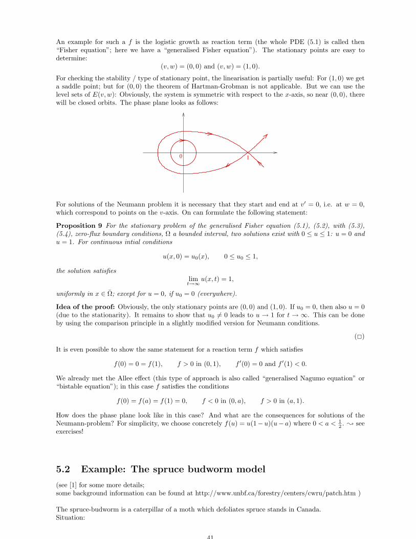
An example for such a f is the logistic growth as reaction term (the whole PDE (5.1) is called then“Fisher equation”; here we have a “generalised Fisher equation”). The stationary points are easy todetermine:
(v, w) = (0, 0) and (v, w) = (1, 0).
For checking the stability / type of stationary point, the linearisation is partially useful: For (1, 0) we geta saddle point; but for (0, 0) the theorem of Hartman-Grobman is not applicable. But we can use thelevel sets of E(v, w): Obviously, the system is symmetric with respect to the x-axis, so near (0, 0), therewill be closed orbits. The phase plane looks as follows:
0 1
For solutions of the Neumann problem it is necessary that they start and end at v′ = 0, i.e. at w = 0,which correspond to points on the v-axis. On can formulate the following statement:
Proposition 9 For the stationary problem of the generalised Fisher equation (5.1), (5.2), with (5.3),(5.4), zero-flux boundary conditions, Ω a bounded interval, two solutions exist with 0 ≤ u ≤ 1: u = 0 andu = 1. For continuous intial conditions
u(x, 0) = u0(x), 0 ≤ u0 ≤ 1,
the solution satisfieslim
t→∞u(x, t) = 1,
uniformly in x ∈ Ω; except for u = 0, if u0 = 0 (everywhere).
Idea of the proof: Obviously, the only stationary points are (0, 0) and (1, 0). If u0 = 0, then also u = 0(due to the stationarity). It remains to show that u0 6= 0 leads to u → 1 for t → ∞. This can be doneby using the comparison principle in a slightly modified version for Neumann conditions.
(2)
It is even possible to show the same statement for a reaction term f which satisfies
f(0) = 0 = f(1), f > 0 in (0, 1), f ′(0) = 0 and f ′(1) < 0.
We already met the Allee effect (this type of approach is also called “generalised Nagumo equation” or“bistable equation”); in this case f satisfies the conditions
f(0) = f(a) = f(1) = 0, f < 0 in (0, a), f > 0 in (a, 1).
How does the phase plane look like in this case? And what are the consequences for solutions of theNeumann-problem? For simplicity, we choose concretely f(u) = u(1− u)(u− a) where 0 < a < 1
2 . ; seeexercises!
5.2 Example: The spruce budworm model
(see [1] for some more details;some background information can be found at http://www.unbf.ca/forestry/centers/cwru/patch.htm )
The spruce-budworm is a caterpillar of a moth which defoliates spruce stands in Canada.Situation:
41
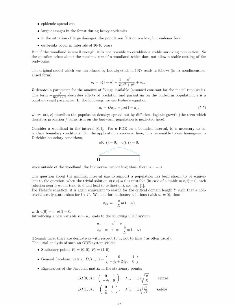
• epidemic spread-out
• large damages in the forest during heavy epidemics
• in the situation of large damages, the population falls onto a low, but endemic level.
• outbreaks occur in intervals of 30-40 years
But if the woodland is small enough, it is not possible to establish a stable surviving population. Sothe question arises about the maximal size of a woodland which does not allow a stable settling of thebudworms.
The original model which was introduced by Ludwig et al. in 1978 reads as follows (in its nondimension-alised form):
ut = u(1 − u) − 1
R
u2
ε2 + u2+ uxx.
R denotes a parameter for the amount of foliage available (assumed constant for the model time-scale).
The term − u2
R(ε2+u2) describes effects of predation and parasitism on the budworm population; ε is a
constant small parameter. In the following, we use Fisher’s equation:
ut = Duxx + µu(1 − u), (5.5)
where u(t, x) describes the population density; spread-out by diffusion, logistic growth (the term whichdescribes predation / parasitism on the budworm population is neglected here).
Consider a woodland in the interval [0, l]. For a PDE on a bounded interval, it is necessary to in-troduce boundary conditions. For the application considered here, it is reasonable to use homogeneousDirichlet boundary conditions,
u(0, t) = 0, u(l, t) = 0,
0 lsince outside of the woodland, the budworms cannot live; thus, there is u = 0.
The question about the minimal interval size to support a population has been shown to be equiva-lent to the question, when the trivial solution u(x, t) = 0 is unstable (in case of a stable u(x, t) ≡ 0, eachsolution near 0 would tend to 0 and lead to extinction), see e.g. [1].For Fisher’s equation, it is again equivalent to search for the critical domain length l∗ such that a non-trivial steady state exists for l > l∗. We look for stationary solutions (with ut = 0), thus
uxx = − µ
Du(1 − u)
with u(0) = 0, u(l) = 0.Introducing a new variable v := ux leads to the following ODE system:
ux = u′ = v
vx = v′ = − µ
Du(1 − u)
(Remark here, there are derivatives with respect to x, not to time t as often usual).The usual analysis of such an ODE-system yields:
• Stationary points P1 = (0, 0), P2 = (1, 0)
• General Jacobian matrix: Df(u, v) =
(0 1
− µD + 2 µ
Du 0
)
• Eigenvalues of the Jacobian matrix in the stationary points:
Df(0, 0) :
(0 1
− µD 0
)
, λ1,2 = ±i
õ
Dcentre
Df(1, 0) :
(0 1µD 0
)
, λ1,2 = ±√
µ
Dsaddle
42
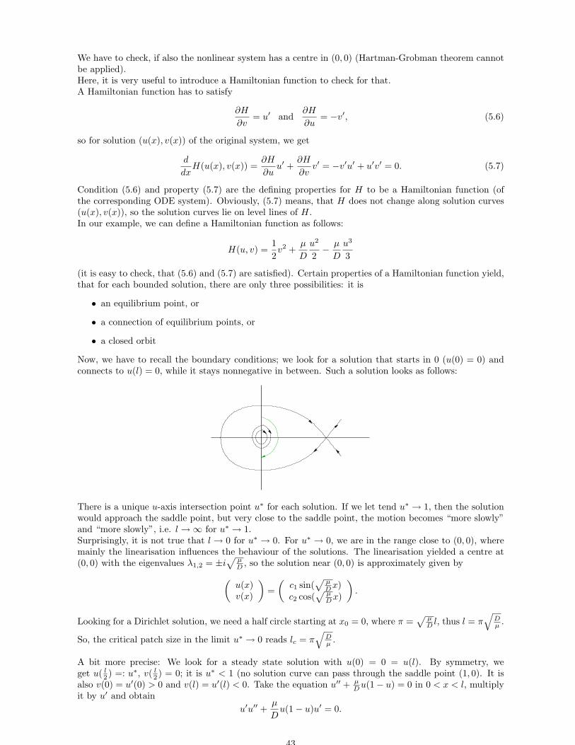
We have to check, if also the nonlinear system has a centre in (0, 0) (Hartman-Grobman theorem cannotbe applied).Here, it is very useful to introduce a Hamiltonian function to check for that.A Hamiltonian function has to satisfy
∂H
∂v= u′ and
∂H
∂u= −v′, (5.6)
so for solution (u(x), v(x)) of the original system, we get
d
dxH(u(x), v(x)) =
∂H
∂uu′ +
∂H
∂vv′ = −v′u′ + u′v′ = 0. (5.7)
Condition (5.6) and property (5.7) are the defining properties for H to be a Hamiltonian function (ofthe corresponding ODE system). Obviously, (5.7) means, that H does not change along solution curves(u(x), v(x)), so the solution curves lie on level lines of H.In our example, we can define a Hamiltonian function as follows:
H(u, v) =1
2v2 +
µ
D
u2
2− µ
D
u3
3
(it is easy to check, that (5.6) and (5.7) are satisfied). Certain properties of a Hamiltonian function yield,that for each bounded solution, there are only three possibilities: it is
• an equilibrium point, or
• a connection of equilibrium points, or
• a closed orbit
Now, we have to recall the boundary conditions; we look for a solution that starts in 0 (u(0) = 0) andconnects to u(l) = 0, while it stays nonnegative in between. Such a solution looks as follows:
There is a unique u-axis intersection point u∗ for each solution. If we let tend u∗ → 1, then the solutionwould approach the saddle point, but very close to the saddle point, the motion becomes “more slowly”and “more slowly”, i.e. l → ∞ for u∗ → 1.Surprisingly, it is not true that l → 0 for u∗ → 0. For u∗ → 0, we are in the range close to (0, 0), wheremainly the linearisation influences the behaviour of the solutions. The linearisation yielded a centre at(0, 0) with the eigenvalues λ1,2 = ±i
õD , so the solution near (0, 0) is approximately given by
(u(x)v(x)
)
=
(c1 sin(
õD x)
c2 cos(√
µDx)
)
.
Looking for a Dirichlet solution, we need a half circle starting at x0 = 0, where π =√
µD l, thus l = π
√Dµ .
So, the critical patch size in the limit u∗ → 0 reads lc = π√
Dµ .
A bit more precise: We look for a steady state solution with u(0) = 0 = u(l). By symmetry, weget u( l
2 ) =: u∗, v( l2 ) = 0; it is u∗ < 1 (no solution curve can pass through the saddle point (1, 0). It is
also v(0) = u′(0) > 0 and v(l) = u′(l) < 0. Take the equation u′′ + µDu(1 − u) = 0 in 0 < x < l, multiply
it by u′ and obtain
u′u′′ +µ
Du(1 − u)u′ = 0.
43

Integrating this equation yields
u′2
2+
µ
D
u2
2− µ
D
u3
3︸ ︷︷ ︸
=:F (u)
= A︸︷︷︸
=:F (u∗)
(= const.)
(the integration constant can be chosen arbitrarily, hence also as F (u∗)).This can be solved for u′:
u′ =
√
2(F (u∗) − F (u)) for 0 ≤ x ≤ l2
−√
2(F (u∗) − F (u)) for l2 ≤ x ≤ l,
then the sign of u′ fits to the requirement.Integrating this from x to l
2 yields (for 0 < x < l2 ):
l
2− x =
∫ l2
x
1 dy =
∫ l2
x
u′√
2(F (u∗) − F (u))dy
=
∫ u( l2)
u(x)
1√
2(F (u∗) − F (z))dz
=
∫ u∗
u(x)
1√
2(F (u∗) − F (z))dz.
For l2 < x < l we get similarly by integrating
∫ l2
x
− u′√
2(F (u∗) − F (u))dy =
∫ l2
x
1 dy
⇔∫ u∗
u(x)
1√
2(F (u∗) − F (z))dz = x − l
2,
which corresponds to (in general)∫ u∗
u(x)
1√
2(F (u∗) − F (z))dz =
∣∣∣∣x − l
2
∣∣∣∣.
If µ is known, this is an implicit equation for u.The boundary conditions claim u(0) = u(l) = 0, hence for x = 0 and/or x = l:
∫ u∗
0
1√
2(F (u∗) − F (z))dz =
l
2⇔ l =
√2
∫ u∗
0
1√
F (u∗) − F (z))dz.
Due to monotonicity etc., the length l of the domain uniquely determines u∗. It can be interpreted as“given a non-trivial solution with max. value u∗, how long is the corresponding length l of the domain?”Minimally, we can have u∗ → 0. So we determine
lc = limu∗→0
√2
∫ u∗
0
1√
F (u∗) − F (z)dz
= limu∗→0
√2
∫ u∗
0
1√
− µD
z2
2 + µD
z3
3 + µD
u∗2
2 − µD
u∗3
3
dz
= limu∗→0
2√
µD
∫ u∗
0
1√
−z2 + 23z3 + u∗2 − 2
3u∗3dz
= limu∗→0
2
√
D
µ
∫ u∗
0
dz√u∗2 − z2
= limu∗→0
2
√
D
µ
[
arcsinz
u∗
]u∗
0
=
√
D
µπ.
The graph of u∗, dependent on l looks as follows:
44
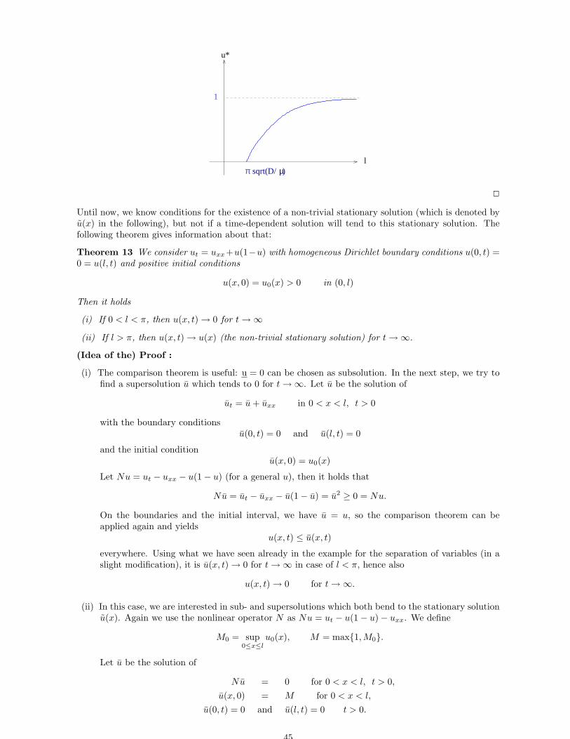
l
u*
π
1
sqrt(D/ )µ
2
Until now, we know conditions for the existence of a non-trivial stationary solution (which is denoted byu(x) in the following), but not if a time-dependent solution will tend to this stationary solution. Thefollowing theorem gives information about that:
Theorem 13 We consider ut = uxx +u(1−u) with homogeneous Dirichlet boundary conditions u(0, t) =0 = u(l, t) and positive initial conditions
u(x, 0) = u0(x) > 0 in (0, l)
Then it holds
(i) If 0 < l < π, then u(x, t) → 0 for t → ∞
(ii) If l > π, then u(x, t) → u(x) (the non-trivial stationary solution) for t → ∞.
(Idea of the) Proof :
(i) The comparison theorem is useful: u = 0 can be chosen as subsolution. In the next step, we try tofind a supersolution u which tends to 0 for t → ∞. Let u be the solution of
ut = u + uxx in 0 < x < l, t > 0
with the boundary conditionsu(0, t) = 0 and u(l, t) = 0
and the initial conditionu(x, 0) = u0(x)
Let Nu = ut − uxx − u(1 − u) (for a general u), then it holds that
Nu = ut − uxx − u(1 − u) = u2 ≥ 0 = Nu.
On the boundaries and the initial interval, we have u = u, so the comparison theorem can beapplied again and yields
u(x, t) ≤ u(x, t)
everywhere. Using what we have seen already in the example for the separation of variables (in aslight modification), it is u(x, t) → 0 for t → ∞ in case of l < π, hence also
u(x, t) → 0 for t → ∞.
(ii) In this case, we are interested in sub- and supersolutions which both bend to the stationary solutionu(x). Again we use the nonlinear operator N as Nu = ut − u(1 − u) − uxx. We define
M0 = sup0≤x≤l
u0(x), M = max1,M0.
Let u be the solution of
Nu = 0 for 0 < x < l, t > 0,
u(x, 0) = M for 0 < x < l,
u(0, t) = 0 and u(l, t) = 0 t > 0.
45
This solution u satisfies Nu = 0 ≥ 0 = Nu, u(0, t) = 0 ≥ 0 = u(0, t), u(l, t) = 0 ≥ 0 = u(l, t) andu(x, 0) = M ≥ M0 ≥ u(x, 0); hence u is indeed a supersolution of the problem for u and we get thatu(x, t) ≥ u(x, t) for 0 ≤ x ≤ l and t ≥ 0 by the comparison theorem. In the next step we need toshow that u is monotone decreasing (and hence tends to a limit), i.e. u(x, t) ≥ u(x, t + h). DefineUh(x, t) = u(x, t) for any fixed h. Uh satisfies:
NUh = 0 for 0 < x < l, t > 0
Uh(x, 0) = u(x, h) for 0 < x < l
Uh(0, t) = 0 and Uh(l, t) = 0 for t > 0.
Hence, Uh is a subsolution of the problem for u in case of Uh(x, 0) ≤ u(x, 0). Due to u(x, t) ≤ Mfor all t, it is also
Uh(x, 0) = u(x, h) ≤ M = u(x, 0),
and it follows thatu(x, t + h) = Uh(x, t) ≤ u(x, t) for allx, t,
i.e. u is monotone decreasing. As it is bounded below by zero, limt→∞ u(x, t) = w(x) exists and it is0 ≤ w(x) ≤ M . With some more analytical tools one can show (see Aronson and Weinberger, 1975,1978) that indeed w(x) is a non-negative solution of ut = u(1 − u) + uxx satisfying the boundaryconditions u(0, t) = u(l, t) = 0.Next, it is necessary to show that w is non-zero: Remember that there is a unique positive solutionu(x) ; so we can use the comparison theorem (it is Nu = 0 with zero boundary conditions andinitial conditions u(x) ≤ 1 ≤ M = u(x, 0)), which yields u(x, t) = u(x), thus also w(x) ≥ u(x). Butu(x) is the unique positive solution of the given problem, so it follows that
w(x) = u(x), ; limt→∞
u(x, t) = u(x).
In a similar, but slightly more complicated way, one can construct a subsolution u(x, t) whichbounds u(x, t) from below. For this subsolution u(x, t) it can be shown that
limt→∞
u(x, t) = u(x).
Altogether, this yields u ≤ u ≤ u andlim
t→∞u(x, t) = u(x).
This means that for l > π, the stationary solution u(x, t) = u(x) of the logistic equation in (0, l) withzero boundary conditions and positive initial conditions is globally attracting.
2
For the original spruce-budworm model, similar calculations can be done (just more complex) and yieldfinally
Theorem 14 For the spruce-budworm equation,
ut = u(1 − u) − 1
R
u2
ε2 + u2+ uxx for x ∈ (0, l),
with the boundary conditionsu(0, t) = 0 = u(l, t),
no stationary solutions exists if l < π. In case of l > π, there are stationary solutions of the followingform:
(i) For small R (R < R1), there exists one non-trivial solution, which is at endemic level and stable.
(ii) For larger R (R1 < R < R2), the stable solution at the endemic level still exists for all l > π,but for l > l1(R) a second stable solution appears at the so-called epidemic level; between these twostable solutions, there is an unstable solution.
(iii) For larger R (R2 < R < R3), the solution at the endemic level disappears for l > l2(R). (Itdepends on the initial conditions to which stable solution the solution tends to)
46
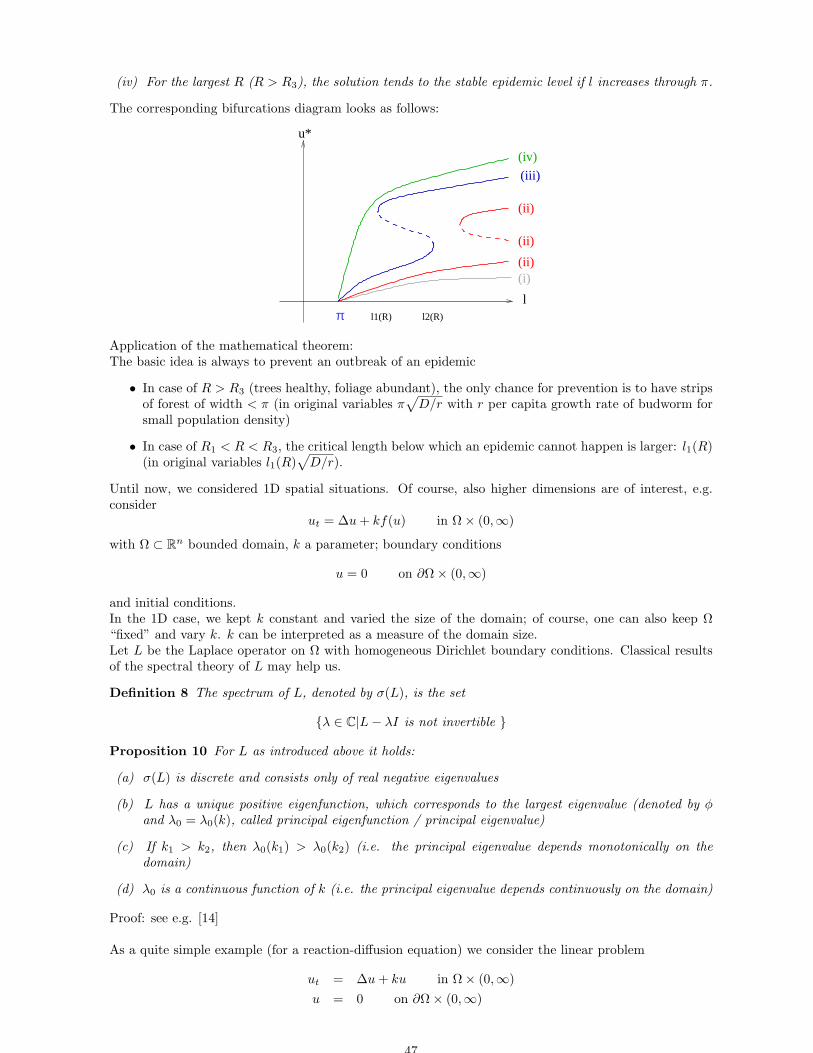
(iv) For the largest R (R > R3), the solution tends to the stable epidemic level if l increases through π.
The corresponding bifurcations diagram looks as follows:
l
u*
π
(iii)
(iv)
(ii)
(ii)
(ii)
(i)
l1(R) l2(R)
Application of the mathematical theorem:The basic idea is always to prevent an outbreak of an epidemic
• In case of R > R3 (trees healthy, foliage abundant), the only chance for prevention is to have stripsof forest of width < π (in original variables π
√
D/r with r per capita growth rate of budworm forsmall population density)
• In case of R1 < R < R3, the critical length below which an epidemic cannot happen is larger: l1(R)(in original variables l1(R)
√
D/r).
Until now, we considered 1D spatial situations. Of course, also higher dimensions are of interest, e.g.consider
ut = ∆u + kf(u) in Ω × (0,∞)
with Ω ⊂ Rn bounded domain, k a parameter; boundary conditions
u = 0 on ∂Ω × (0,∞)
and initial conditions.In the 1D case, we kept k constant and varied the size of the domain; of course, one can also keep Ω“fixed” and vary k. k can be interpreted as a measure of the domain size.Let L be the Laplace operator on Ω with homogeneous Dirichlet boundary conditions. Classical resultsof the spectral theory of L may help us.
Definition 8 The spectrum of L, denoted by σ(L), is the set
λ ∈ C|L − λI is not invertible
Proposition 10 For L as introduced above it holds:
(a) σ(L) is discrete and consists only of real negative eigenvalues
(b) L has a unique positive eigenfunction, which corresponds to the largest eigenvalue (denoted by φand λ0 = λ0(k), called principal eigenfunction / principal eigenvalue)
(c) If k1 > k2, then λ0(k1) > λ0(k2) (i.e. the principal eigenvalue depends monotonically on thedomain)
(d) λ0 is a continuous function of k (i.e. the principal eigenvalue depends continuously on the domain)
Proof: see e.g. [14]
As a quite simple example (for a reaction-diffusion equation) we consider the linear problem
ut = ∆u + ku in Ω × (0,∞)
u = 0 on ∂Ω × (0,∞)
47
Let λi be the eigenvalues of L, then the eigenvalues of the linear problem are given by µi = k + λi. Thenthe largest eigenvalue is k + λ0(k).Let’s have a short excurs to linear problems, written as
vt = Av,
where A is a linear differential operator defined on a suitable function space which satisfies the prescribedboundary conditions. As in the preceding chapter, the definition domain of A, D(A) can be extended toa dense subset of an Banach space X (e.g. L2(Ω)), which allows us to use the X-Norm. An steady stateu0 is asymptotically stable, if ‖v‖X → 0 for t → ∞. If the spectrum of A is contained completely in theleft half space of the complex plane (i.e. Re(λ) ≤ β for a β < 0 for all λ ∈ σ(A)). One can show that inthis case ‖v‖X decays like eβt. The idea behind is easy to see: For simple initial-boundary-value problemson compact domains, σ(A) consists of a sequence of eigenvalues λm, with corresponding eigenfunctionswhich satisfy
Aφm = λφm.
If there exists a m ∈ N such that Re(λm) ≥ 0, then we get for an initial condition of the form
v(x, 0) = const · φm(x)
the solutionv(x, t) = const · eλmtφm(x).
But such a v(x, t) does not approach zero for t → ∞, i.e. zero is unstable in this case.Vice versa: As already known, the function space which contains the solutions v is spanned by theeigenfunctions, any solution can be written in the following way:
v(x, t) =∞∑
m=1
am(t)φm(x).
This leads (via vt = Av) to the condition for the coefficients am(t):
dam
dt= λmam
Hence λm < 0 is needed for each m to get v → 0 for t → ∞.(Remark that similar considerations can be done in case of an unbounded Ω, but becomes more com-plicated due to a more complicated spectrum - not only with discrete eigenvalues, such a continuum iscalled “essential spectrum”, but the latter one depends essentially on the choice of function space forpossible initial values for v)
Back to our problem ut = ∆u + ku; now we know:If λ0(k) < −k (which corresponds to a sufficiently small domain Ω), then all eigenvalues µ are negative,resulting in a stable steady state 0.If λ0(k) > −k (which corresponds to a sufficiently large domain Ω), then µ0 = k + λ0(k) > 0 and thesteady state is unstable.
In the next step, we show that the stability of the trivial solution of a corresponding nonlinear problemcan be examined by a linear stability analysis (somehow analogous to Hartman-Grobman theorem forODEs).
Theorem 15 (Principle of Linearised Stability) Consider
ut = ∆u + ku + h(u) in Ω × (0,∞)
u = 0 on ∂Ω × (0,∞)
u(x, 0) = u0(x),
where h(0) = 0, h′(0) = 0. Let λ0 = λ0(k) be the principal eigenvalue in σ(L).If λ0 < −k, then the trivial steady state is stable.If λ0 > −k, then it is unstable.
48
Proof: Let λ0 < −k. We aim to find a supersolution of the problem which tends to zero for t → ∞.From Prop. 10 it is known: the principal eigenvalue of L depends continuously and monotonically on thedomain (k), so it is possible to find a k′ > k satisfying λ0(k) < λ0(k
′) < −k. Let u(x, t) be the solutionof
ut = ∆u + k′u in Ω × (0,∞)
u = 0 on ∂Ω × (0,∞)
u(x, 0) = u0(x)
Considering the eigenvalues of this problem yields that u is monotone decreasing and indeed tends tozero for t → ∞. Due to the definitions we find:
Nu = ut − ku − h(u) − ∆u = (k′ − k)u − h(u).
It is k′ > k, so there exists a ε > 0 such that
(k′ − k)u − h(u) ≥ 0 ∀u ∈ (0, ε)
If u0 satisfies the inequality u0(x) ≤ ε for all x ∈ Ω, then we get u(x, t) ≤ u0(x) ≤ ε (as u is monotonedecreasing) and
Nu ≥ 0
(due to (k′ − k)u − h(u) ≥ 0)Hence, u is a supersolution of the problem for u which tends to zero; we get that the trivial solution isindeed asymptotically stable.
The instability of the trivial solution in case of λ0 > −k can be shown in a similar way (left out here).
2
By such an approach, the existence of a non-trivial steady state solution for the logistic equation can beshown:
Theorem 16 If λ0 > −k, then
ut = ∆u + ku(1 − u) in Ω × (0,∞)
u = 0 on ∂Ω × (0,∞)
possesses at least one non-trivial nonnegative steady state solution.
Idea of the proof: Again we use sup- and supersolutions. Let δ > 0 and let φ be the principaleigenfunction of L, i.e. ∆φ = λ0φ with λ0 + k > 0 (according to the assumption), φ > 0 in Ω (accordingto Prop. 10) and φ = 0 on ∂Ω.Let u = δφ, then it satisfies
ut − ku(1 − u) − ∆u = −λ0δφ − kδφ(1 − δφ)
= −(λ0 + k)δφ + δ2kφ2
≤ 0
for a sufficiently small δ; of course u = 0 on ∂Ω × (0,∞), so u is a subsolution.For a supersolution we can take u = 1. Obviously it is
Nu = ut − ∆u − ku(1 − u) = 0 in Ω
and u ≥ 0 on ∂Ω × (0,∞) . Similar to Theorem 13, the existence of a steady-state solution v(x) withu(x) ≤ v(x) ≤ u(x) can be shown.
(2)
Remark: For the budworm equation, a similar statement can be shown.
49
Chapter 6
Reaction-diffusion systems
6.1 What can be expected from Reaction-diffusion systems?
Reference. [12]
In general, systems of reaction-diffusion equations allow for much more complex behaviour than a scalarreaction-diffusion equation does. Especially interacting reaction terms are of interest and lead to inter-esting behaviour. So, e.g. oscillating phenomena can evolve - as these oscillations can spread in spacevia diffusion and instabilities may develop spatial phenomena like pattern formation can be observed andobserved. We will see some of the typical examples below.Furthermore, the analysis and general statements become more difficult; not all properties which arewell-known from the scalar case can be directly transferred to systems.
6.2 Conservative systems
Reference: [1]
We start to consider a special kind of reaction-diffusion systems, the so-called conservative systems,which means: the reaction terms are “conservative”. Generally, for a conservative system, a functionof the dependent variables exists, which is a constant of the motion; it can be interpreted as a kind of“energy”. Mathematically formulated:System u = f(u) (m-dimensional) is conservative if a function G(u) exists with
G(u) =
m∑
i=1
∂G
∂uiui =
m∑
i=1
∂G
∂uifi(u) = 0.
Of course, such conservative systems have special properties; e.g. they often have oscillatory solutions.Often, they are “easy” to analyse, but from a modelling point of view, there are also disadvantages, ase.g. structural instability (as known from the classical predator-prey model).
6.2.1 Lotka-Volterra system
Nevertheless, we consider here the classical predator-prey model; let’s start with the non-dimensionalisedversion
u = u(1 − v) (6.1)
v = av(u − 1) (6.2)
Already known: stationary points are (0, 0) (saddle-point; via linearisation), (1, 1) (centre in the linearisedsystem, but as Hartman-Grobman is not applicable in that case, additional analysis needed). System(6.1), (6.2) can be separated for the variables, i.e. first we get
av(u − 1) du = u(1 − v) dv,
then
au − 1
udu =
v − 1
vdv,
50
which can be integrated and yields
G(u, v) = a(u − lnu) + v − ln v = A(const.)
This is already known (also that solutions curves are contained in level sets of G(u, v), and can beinterpreted in this context as “the quantity G(u, v) is conserved”, thus the Lotka-Volterra system is con-servative.A first interesting question concerns small perturbations of the system and how they influence the be-haviour of such a system. E.g. if we like to introduce a self-limitation of the prey population, the systemlooks as follows:
u = u(1 − v)εu2
v = av(u − 1)
Even though ε can be assumed very small, there is a significant effect on the behaviour of the system: thecoexistence point (now (1, 1− ε) becomes a stable spiral, and V (u, v) = a(u− lnu) + v − (1− ε) a globalLyapunov function, no periodic solutions present anymore. From a biological point of view this means:even a small perturbation could remove the oscillations, which isn’t too realistic. From a mathematicalpoint of view, such a behaviour is called “structural instability”. Remark, that all conservative systemsare structurally unstable. Nevertheless they are interesting to consider as they may teach us about theinfluences of simple interactions.Next we consider the Lotka-Volterra system including diffusion for both species (with equal diffusioncoefficients) and find some information about the long time behaviour of the solution.
Theorem 17 (Murray, 1975) The diffusional Lotka-Volterra system,
ut = u(1 − v) + D∆u
vt = av(u − 1) + D∆u
with equal diffusion coefficients and homogeneous Neumann boundary conditions
∂u
∂n(x, t) = 0 =
∂v
∂n(x, t) on x ∈ ∂Ω
(n the outward normal; Ω bounded subset of Rn) tends to a spatially uniform state for t → ∞.
Proof: Let the initial conditions be
u(x, 0) = u0(x), v(x, 0) = v0(x) for x ∈ Ω.
We define s(x, t), corresponding to the “energy” of the system without diffusion,
s = a(u − lnu) + v − ln v, (6.3)
i.e. for D = 0 it satisfies st = 0. Question: How does the corresponding differential equation for s looklike for D 6= 0?We take (6.3) and differentiate it:
st = a(
ut −ut
u
)
+ vt −vt
v
∆s = a
(
∆u − ∆u
u+
|∇u|2u2
)
+ ∆v − ∆v
v+
|∇v|2v2
,
this yields
st − D∆s = a(ut − D∆u)u − 1
u+ (vt − D∆v)
v − 1
v− aD|∇u|2/u2 − D|∇v|2/v2
= −aD|∇u|2/u2 − D|∇v|2/v2 ≤ 0.
using the system equations. This can be interpreted in such a way that the energy is dissipated by thediffusion terms.The boundary conditions for s are
∂s
∂n(x, t) = 0 for x ∈ ∂Ω
51
and the initial condition reads
s(x, 0) = a(u0 − lnu0) + v0 − ln v0 = s0(x).
(Both follow directly from the conditions for u and v) Via integration over Ω we can define the “totalamount of energy” in the system at time t:
S(t) =
∫
Ω
s(x, t) dx.
Using the Neumann boundary condition and Green formula yields
S(t) =
∫
Ω
D∆s dx
︸ ︷︷ ︸
=DR
∂Ω∂S∂n
ds=0
+
∫
Ω
−aD|∇u|2
u2− D
|∇v|2v2
dx
= −D
∫
Ω
a|∇u|2u2
+|∇v|2
v2dx.
Obviously, S is monotone non-increasing; there are two possibilities: it tends to a finite limit or it tendsto −∞ for t → ∞. By definition, s satisfies s(x, t) ≥ a + 1, from which we get directly
S(t) =
∫
Ω
s(x, t) dx ≥ (a + 1)|Ω|,
so S indeed tends to a finite limit, which requires
S = −D
∫
Ω
a|∇u|2u2
+|∇v|2
v2dx → 0.
The only possibility to satisfy this, is that also ∇u and ∇v tend to 0 for t → ∞, i.e. the system tends toa spatially uniform state.
2
Remark: The result can be also generalised to the case of two differential diffusion coefficients.
What does this theorem mean? The Lotka-Volterra system, even if including diffusion, cannot yieldecological patchiness; no spatial distribution of species in a environment in possible in the long time run.
6.3 Some more basics for Reaction-diffusion systems
Reference: [1]
We learnt already much about properties and useful theorems for (mainly scalar) reaction diffusionequations. Some results can be extended to reaction-diffusion systems, but one has to be careful aboutthe assumptions, and some statements are weaker.
Remark: In the following, order relations, operators like max,min, sup, inf and also the typical propertiesof solutions and inequalities are defined and interpreted component wise.To be able to formulate the results in a quite general way, we use the following definition for the boundaryconditions:
Definition 9 (Boundary operator) The boundary operator B is defined by
(Bu)i = ci(x, t)ui(x, t) + di(x, t)∂ui
∂νi(x, t),
where (Bu)i denotes component i of the vector Bu, ci ≥ 0, di ≥ 0, c2i + d2
1 > 0 and ∂∂νi
denotes anyoutward derivative. Remark: B is a diagonal operator, i.e. (Bu)i only depends on component i of u.
Now we can introduce an invariant set:
52
Definition 10 (Invariant set) An invariant set of the (spatially homogeneous) system ut = f(u) is aset Σ ⊂ R
m (m dimension of u), such that if u is a solution of ut = f(u) in 0 < t < T for an T ≤ ∞with initial conditions u(0) ∈ Σ, then the solution stays in Σ, i.e. u(t) ∈ Σ for 0 ≤ t ≤ T . In the sameway, an invariant set for the initial boundary value problem is a set Σ ⊂ R
m such that if u is a solutionof
ut = f(u) + ∆u in Ω × (0, T )
with all initial and boundary values in Σ, then also u(x, t) ∈ Σ is satisfied for all x ∈ Ω and 0 ≤ t < T .
Next, monotonicity is generalised for the higher-dimensional case:
Definition 11 A function f(u) is called quasi-monotone nondecreasing, if each component fi(u) is non-decreasing in uj for each j 6= i.f(u) is called to possess the mixed quasi-monotone property, if each component fi(u) is monotone in uj
for each j 6= i.
In the following, we consider system which can be written in the following form:
Nu = Lu − f(u) = ut − D∆u − f(u) = 0 in Ω × (0, T ] (6.4)
u(x, 0) = uo(x) on Ω × 0 (6.5)
Bu = b(x, t) on ∂Ω × (0, T ) (6.6)
Additional requirements:
• D is the so-called diagonal diffusion matrix (not all entries of the diagonal should be = 0)
• B is a diagonal boundary operator
This system (6.4)-(6.6) is called “problem (P)” in this section. The comparison theorem can also begeneralised for systems and formulated in the following way:
Theorem 18 (Comparison theorem) Let the following assumptions hold:
(i) u and u are sub- resp. supersolutions of problem (P)
(ii) f is uniformly Lipschitz continuous in u
(iii) Ω × (0, T ) satisfies the so-called “interior sphere property” (except for we deal with the Dirichletproblem); this means: a closed ball exists, which is contained in Ω × (0, T ) and only intersects theboundary at one single point
(iv) f is quasi-monotone non-decreasing
Then it is (according to the weak comparison theorem):
u ≤ u in Ω × [0, T ]
The strong comparison theorem yields:For each i one of the two following possibilities holds:
(a) ui < ui in Ω × (0, T ]
(b) ui = ui in Ω × (0, t∗] for a t∗ ≤ T .
Rough idea of the proof: The scalar maximum principle is applied to the function wi = ui − ui + y,by that one can show that wi > 0, where y (also a function) depends on a parameter ε and y → 0 forε → 0. For the necessary estimates, Lipschitz continuity and the restrictions for f are used. For thestrong comparison theorem, the scalar strong maximum principle is applied.
(2)
Remark that the possible interactions of the components via the reaction term f lead to these restrictionsfor f .
The following corollary gives information about invariant sets:
53
Corollary 2 Let assumptions (ii)-(iv) of Theorem 18 hold. Let a, b be constant vectors satisfying −∞ ≤a ≤ b ≤ ∞ and f(a) ≥ 0, f(b) ≤ 0. Then Σ = u|a ≤ u ≤ b is an invariant set for problem (P).
With these assumptions, it is quite easy to show global existence of a solution!
Theorem 19 (Global existence) Let assumptions (ii)-(iv) of Theorem 18 hold. If there exists aninvariant set Σ = u|a ≤ u ≤ b for problem (P), then Problem (P) has a solution for all times.
Proof: Let K be the Lipschitz constant for the reaction function f . Let Li denote the differentialoperator for component i, i.e.
Livi =∂vi
∂t− Di∆vi
Two sequences vn and wn are defined in the following way:
v0 = a, (Li + K)vni = fi(v
n−1) + Kvn−1i
w0 = b, (Li + K)wni = fi(w
n−1) + Kwn−1i
with the boundary and initial conditions (6.5) and (6.6). It is necessary that aA and b are finite!To show: vn+1 − vn ≥ 0 by inductionStart n = 0: There we find
(Li + K)(v1i − v0
i ) = fi(v0) + Kv0
i − Liv0i − Kv0
i
= −(Liv0i
︸︷︷︸
=0
−fi(v0)) = fi(a) ≥ 0.
The scalar maximum principle yields v1i − v0
i ≥ 0 (as the initial and boundary conditions have to besatisfied by both).Induction step: Assume that the statement is already shown for n − 1. We get
(Li + K)(vn+1i − vn
i ) = fi(vn) + Kvn
i − fi(vn−1) − Kvn−1
i
≥ −K(vni − vn−1
i ) + K(vni − vn−1
i ) = 0
(this is valid since f is Lipschitz continuous and quasi-monotone non-decreasing). Applying again thescalar maximum principle yields vn+1 − vn
i ≥ 0 as desired.Similarly, for wn can be shown: wn+1 − wn ≤ 0.Now we have a monotonic increasing vn and a monotonic decreasing wn, the limits v = limn→∞ vn
and w = limn→∞ wn exists. But as there is only a unique solution of the problem, it is v = w.
2
Remark: The required quasi-monotonicity is essential. As an example, we consider:
ut = u + uxx
vt = −u + v + vxx
in the area (x1, x2)× (0,∞), with the initial conditions u = u0, v = v0 (both constant) and homogeneousNeumann boundary conditions ux = vx = 0. The solution can be explicitely written as
u = u0et
v = −u0tet + v0e
t
Obviously, if we increase u0 (the initial condition), u is increased, but v is decreased - “impossible” forthe comparison theorem.
For the next step, we introduce another problem, called (P), defined similar to problem (P), but with areaction term f instead of f , which satisfies f(v) ≤ f(v). In the same way we can introduce a problem(P ) with a super-reaction function f .
Corollary 3 Let f : Rm → R
m be a quasi-monotone non-decreasing uniformly Lipschitz continuousfunction which satisfies f(v) ≤ f(v) for all v ∈ R
m. Let u be a subsolution of (P) and let u be asupersolution of (P). Then it is
u ≤ u in Ω × [0, T ]
54
Proof: According to the assumptions, u is a supersolution of (P), hence it is
Lu ≥ f(u) ≥ f(u),
and then u is a supersolution of (P). The function f has the monotonicity properties; so one can compareu and u and gets u ≤ u.
2
Remark: f itself does not need to have the monotonicity properties. So this is an advantage, comparedto the situation before.
Next question: How to find such a quasi-monotone bounding function f? The following lemma yields apossibility, using an infimum:
Lemma 6 f is defined as follows:
fi(u) = infv|u≤v≤u,vi=ui
fi(v),
where u is a supersolution (can be chosen). Then it is: f(u) ≥ f(u) for all u, the newly constructed fis quasi-monotone non-decreasing, and it is uniformly Lipschitz continuous, if f is Lipschitz continuous(with the same Lipschitz constant).
(without proof here)
Remark: In the same way one can construct f by
fi(u) = supv|u≤v≤u,vi=ui
fi(v)
for a subsolution u.
The next theorem (where we omit again the proof; it contains several sub- and supersolutions, andthe Lipschitz continuity for some estimates) gives a good possibility to get an invariant set; here theso-called invariant rectangles:
Theorem 20 (Invariant Rectangles) Let f be Lipschitz continuous, and Ω×(0, T ) satisfy the interiorsphere property (unless the Dirichlet problem is considered). If −∞ < a < b < ∞ are two constant vectorsin R
m such that
fi(v) ≥ 0 for vi = ai, a ≤ v ≤ b
fi(v) ≤ 0 for vi = bi, a ≤ v ≤ b,
then Σ = v|a ≤ v ≤ b ⊂ Rm is an invariant set for problem (P).
It is even possible to find a global solution with these assumptions:
Theorem 21 (Global existence) Let the assumptions for Theorem 20 be satisfied. Then problem (P)with initial conditions and boundary conditions which are in Σ has a unique global solution.
Proof: not shown here.
These theorems can be useful to show existence of solutions and even find bounds for the solution.
Example: A competition model for two species (Volterra) including diffusion for both species (the nondi-mensionalised version):
∂u1
∂t= u1(1 − u1 − αu2) + D1∆u1 = f1(u1, u2) + D1∆u1 (6.7)
∂u2
∂t= θu2(1 − βu1 − u2) + D2∆u2 = f2(u1, u2) + D2∆u2 (6.8)
in Ω × (0, T ]. homogeneous Neumann boundary conditions
∂u1
∂n(x, t) = 0 =
∂u2
∂n(x, t) on ∂Ω (6.9)
and initial conditions
u1(x, 0) = u1,0(x), u2(x, 0) = u2,0(x) on Ω × 0. (6.10)
55
Theorem 22 Let the initial data (6.10) be nonnegative and bounded, i.e.
0 ≤ (u1,0, u2,0) ≤ M = (M1,M2),
then the competition model with diffusion (6.7),(6.8) with homogeneous Neumann boundary conditions(6.9) has solutions which satisfy
0 ≤ (u1, u2) ≤ b = (b1, b2),
where b1 = max(N1, 1). b2 = max(M2, 1).
Proof: The given a = 0 and b satisfy the required conditions for f in Theorem 20, the invariantrectangles:
f1(a1, u2) = 0 ≥ 0 for a1 = 0
f2(u1, a2) = 0 ≥ 0 for a2 = 0
f1(b1, u2) = b1(1 − b1 − αu2) ≥ 0 since b1 ≥ 1
f2(u1, b2) = θb2(1 − βu1 − b2) ≤ 0 since b2 ≥ 1.
The boundary conditions and the initial conditions also satisfy the requirements, (for the boundaryconditions, we have ∂a
∂n = ∂u∂n = ∂b
∂n = 0 )so indeed Σ = v|a ≤ v ≤ b ⊂ R
2 is an invariant set for the given competition model.
2
56
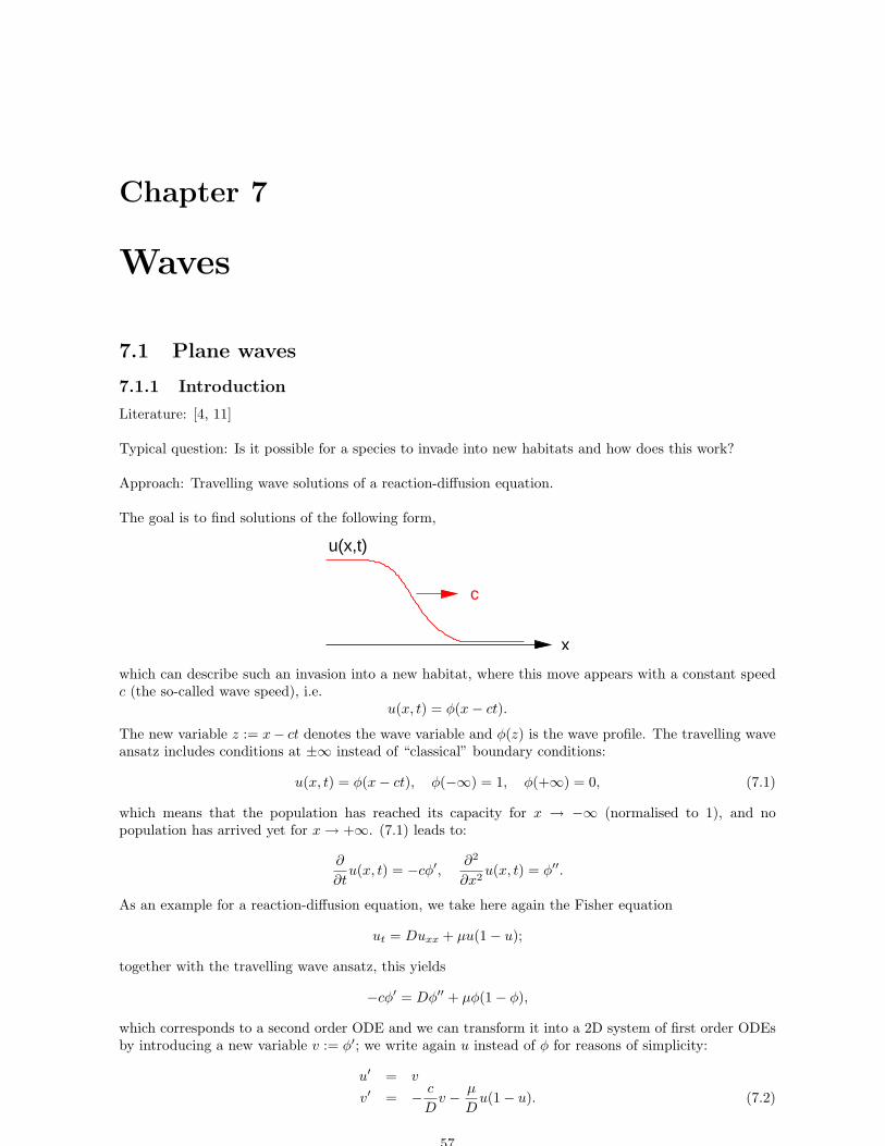
Chapter 7
Waves
7.1 Plane waves
7.1.1 Introduction
Literature: [4, 11]
Typical question: Is it possible for a species to invade into new habitats and how does this work?
Approach: Travelling wave solutions of a reaction-diffusion equation.
The goal is to find solutions of the following form,
u(x,t)
x
c
which can describe such an invasion into a new habitat, where this move appears with a constant speedc (the so-called wave speed), i.e.
u(x, t) = φ(x − ct).
The new variable z := x− ct denotes the wave variable and φ(z) is the wave profile. The travelling waveansatz includes conditions at ±∞ instead of “classical” boundary conditions:
u(x, t) = φ(x − ct), φ(−∞) = 1, φ(+∞) = 0, (7.1)
which means that the population has reached its capacity for x → −∞ (normalised to 1), and nopopulation has arrived yet for x → +∞. (7.1) leads to:
∂
∂tu(x, t) = −cφ′,
∂2
∂x2u(x, t) = φ′′.
As an example for a reaction-diffusion equation, we take here again the Fisher equation
ut = Duxx + µu(1 − u);
together with the travelling wave ansatz, this yields
−cφ′ = Dφ′′ + µφ(1 − φ),
which corresponds to a second order ODE and we can transform it into a 2D system of first order ODEsby introducing a new variable v := φ′; we write again u instead of φ for reasons of simplicity:
u′ = v
v′ = − c
Dv − µ
Du(1 − u). (7.2)
57
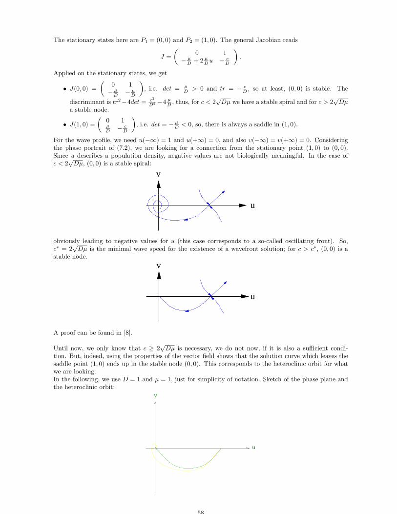
The stationary states here are P1 = (0, 0) and P2 = (1, 0). The general Jacobian reads
J =
(0 1
− µD + 2 µ
Du − cD
)
.
Applied on the stationary states, we get
• J(0, 0) =
(0 1
− µD − c
D
)
, i.e. det = µD > 0 and tr = − c
D , so at least, (0, 0) is stable. The
discriminant is tr2−4det = c2
D2 −4 µD , thus, for c < 2
√Dµ we have a stable spiral and for c > 2
√Dµ
a stable node.
• J(1, 0) =
(0 1µD − c
D
)
, i.e. det = − µD < 0, so, there is always a saddle in (1, 0).
For the wave profile, we need u(−∞) = 1 and u(+∞) = 0, and also v(−∞) = v(+∞) = 0. Consideringthe phase portrait of (7.2), we are looking for a connection from the stationary point (1, 0) to (0, 0).Since u describes a population density, negative values are not biologically meaningful. In the case ofc < 2
√Dµ, (0, 0) is a stable spiral:
v
u
obviously leading to negative values for u (this case corresponds to a so-called oscillating front). So,c∗ = 2
√Dµ is the minimal wave speed for the existence of a wavefront solution; for c > c∗, (0, 0) is a
stable node.
v
u
A proof can be found in [8].
Until now, we only know that c ≥ 2√
Dµ is necessary, we do not now, if it is also a sufficient condi-tion. But, indeed, using the properties of the vector field shows that the solution curve which leaves thesaddle point (1, 0) ends up in the stable node (0, 0). This corresponds to the heteroclinic orbit for whatwe are looking.In the following, we use D = 1 and µ = 1, just for simplicity of notation. Sketch of the phase plane andthe heteroclinic orbit:
u
v
58
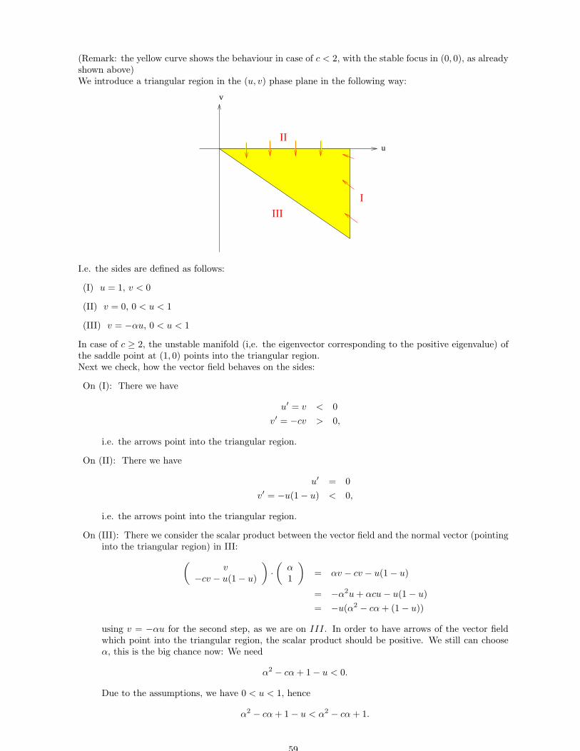
(Remark: the yellow curve shows the behaviour in case of c < 2, with the stable focus in (0, 0), as alreadyshown above)We introduce a triangular region in the (u, v) phase plane in the following way:
u
v
I
II
III
I.e. the sides are defined as follows:
(I) u = 1, v < 0
(II) v = 0, 0 < u < 1
(III) v = −αu, 0 < u < 1
In case of c ≥ 2, the unstable manifold (i,e. the eigenvector corresponding to the positive eigenvalue) ofthe saddle point at (1, 0) points into the triangular region.Next we check, how the vector field behaves on the sides:
On (I): There we have
u′ = v < 0
v′ = −cv > 0,
i.e. the arrows point into the triangular region.
On (II): There we have
u′ = 0
v′ = −u(1 − u) < 0,
i.e. the arrows point into the triangular region.
On (III): There we consider the scalar product between the vector field and the normal vector (pointinginto the triangular region) in III:
(v
−cv − u(1 − u)
)
·(
α1
)
= αv − cv − u(1 − u)
= −α2u + αcu − u(1 − u)
= −u(α2 − cα + (1 − u))
using v = −αu for the second step, as we are on III. In order to have arrows of the vector fieldwhich point into the triangular region, the scalar product should be positive. We still can chooseα, this is the big chance now: We need
α2 − cα + 1 − u < 0.
Due to the assumptions, we have 0 < u < 1, hence
α2 − cα + 1 − u < α2 − cα + 1.
59
So, it is sufficient to choose an α which satisfies
α2 − cα + 1 ≤ 0,
a parabola. To be able to find a positive α which satisfies this inequality, a parabola with twopositive real roots is useful. The roots of the parabola are
α =c ±
√c2 − 4
2,
they are positive and real for c ≥ 2. With these restrictions, we can choose an α, such that thevector fields points into the triangular region, also through III.What happens with the unstable manifold of the saddle point (1,0)? It enters the triangular regionand cannot leave it. There is no stationary point in the interior of the triangular region. A closedorbit can also be excluded, via the negative criterion of Bendixson-Dulac, as we find
div (u, v) =∂v
∂u+
∂(−cv − u(1 − u))
∂v= −c 6= 0.
The only chance is to tend to (0, 0) which corresponds to the heteroclinic orbit, i.e. the travellingwave solution.
Remark 3 For linear parabolic equations like the standard diffusion equation, there are no physicallyrealistic travelling wave solutions; for that purpose it is necessary to “add” a nonlinear term; e.g. theconsidered reaction-diffusion equations can exhibit such solutions. Of course, their form depends on theadditional term f(u).
Until now, we derived only a criterion which gives information about the possible wave speeds, butnothing about the appearance of propagation speeds in the reality. E.g. we can consider the dependencyof the wavespeed c on the initial conditions at infinity (Reference: [11]): When the leading edge of theevolving wave is considered, of course u is small there. An idea could be to neglect there u2 compared tou, so the linearised version of the Fisher equation reads
∂u
∂t=
∂2u
∂x2+ u.
We use an initial condition which behaves like
u(x, 0) ∼ Ae−ax as x → ∞,
a > 0 and A > 0 can be chosen arbitrarily. Now we look for travelling wave solutions for the linearisedequation of the following form:
u(x, t) = Ae−a(x−ct).
This can be interpreted as the leading edge form of the wavefront solution of the nonlinear Fisher equation.Inserting it into the linear equation yields
caAe−a(x−ct) = a2Ae−a(x−ct) + Ae−a(x−ct),
thus there is a relationship between c and a:
ca = a2 + 1 ; c = a +1
a.
If c is interpreted as function of a, it assumes its minimum at a = 1 with cmin = 2; for all other a > 0,the corresponding wave speed is c > 2.Indeed, the asymptotic wave speed for 0 < a ≤ 1 is c = a + 1
a .But for a > 1 something different happens: There it is e−ax < e−x (for positive x), thus also
u(x, t) = A−a(x−ct) < Ae−(x−ct)
According to above, Aex−ct has the wavespeed c = 2, so functions below that cannot spread out fasterthan the “upper bound”. Two cases have to be distinguished:
• 0 < a ≤ 1 ⇒ c = a + 1a
60
• a ≥ 1 ⇒ c = 2
(for more explanation and background see [10])
Next question: How to determine the profile of the travelling wave solution?From the ODE system we get directly: a solution v(u) satisfies
dv
du=
−cv − u(1 − u)
v, (7.3)
thus also the heteroclinic orbit.Let v = 1
cy, then we can rewrite equation (7.3):
εydy
du= −y + u(u − 1), (7.4)
where ε = 1c2 . At least we know that ε is not too big (due to c ≥ 2, so it might make sense to expand y
as a power series in ε:y(u, ε) = y0(u) + εy1(u) + ε2y2(u) + . . .
This is inserted into (7.4):
ε(y0(u) + εy1(u) + ε2y2(u) + . . .) · (dy0
du+ ε
dy1
du+ ε2 dy2
du+ . . .)
= −(y0(u) + εy1(u) + ε2y2(u) + . . .) + u(u − 1).
We split up that equation into the different orders (i.e. powers) in ε:
ε0: y0(u) = u(u − 1)
ε1: y1(u) = −y0(u) · dy0
du
ε2: y2(u) = −y1(u) · dy0
du − y0(u) · dy1
du ,
So, the heteroclinic orbit can be written as
y(u) = y0(u) − ε y0(u)dy0
du︸ ︷︷ ︸
y1(u)
−ε2 y1(u)dy0
du+ y0(u)
dy1
du)
︸ ︷︷ ︸
y2(u)
= u(u − 1) − εu(u − 1)(2u − 1) + . . .
Of course, this can be written also in the original variables u and v:
v(u) = ε1/2(u2 − u) − ε3/2(2u3 − 3u2 + u) + . . .
Now, we have a description in variables u and v. But of course, one is interested more in a solution foru dependent e.g. on z. We can use a similar idea:Let s = z
c , then the wave equation (the ODE of 2nd order) is transformed into
εu′′ + u′ + u(1 − u) = 0. (7.5)
Even though the ε appears in the term with the highest derivative, also for ε = 0 both “additional waveconditions” (u(−∞) = 1 and u(+∞) = 0) can be satisfied also for ε = 0, i.e. we really deal with a regularperturbation problem. Now we can expand u in terms (powers) of ε:
u(s, ε) = u0(s) + εu1(s) + . . . ,
this is substituted in (7.5), we split up the different powers of ε and get:
ε0: u′0 = −u0(1 − u0)
ε1: u′1 + (1 − 2u0)u1 = −u′′
0
61
s can be shifted arbitrarily, since the equation (7.5) and the travelling wave solution both are invariantto translations in s. Thus, we choose s = 0 as point where u = 1/2 for all ε, i.e.
u0 =1
2ui = 0 for i = 1, 2, 3, . . .
Hence, we can solve the equations for the single orders in ε step by step and get
u0(s) =1
1 + es
u1(s) =es
(1 + es)2ln
(4es
(1 + es)2
)
,
and rewritten in the original variable z:
u(z, ε) =1
1 + ez/c+
1
c2
ez/c
(1 + ez/c)2ln
(
4ez/c
(1 + ez/c)
2)
+ O(c−4)
Next step: One can also show that the travelling wave solution for the Fisher equation is stable! This isnot possible (and true) in general (e.g. not under perturbations in the far field, the limit |x| → ∞), bute.g. for the special case of small perturbations of compact support in the “moving coordinate” from ofthe wave.The Fisher equation can be written in the so-called moving coordinate frame; that means: we keep thedependency on t but replace dependency on the spatial variable x by the wave variable z = x − ct:
∂u
∂t= u(1 − u) + c
∂u
∂z+
∂2u
∂z2, (7.6)
i.e. we consider u(x, t) = u(z, t) as the dependent variable.Let c ≥ 2, we assume that there exists a travelling wave solution of the form
u(z, t) = uc(z)
(c arbitrary). As usual, for checking the stability we introduce a small perturbation v(z, t) to uc(z):
u(z, t) = uc(z) + v(z, t). (7.7)
For this perturbation it is assumed that it vanishes outside a finite interval L (in the moving frame), i.e.
v(z, t) = 0 for |z| ≥ L.
Approach (7.7) is inserted into the Fisher equation (in the moving coordinate frame, (7.6)) and yields
∂(uc(z) + v(z, t))
∂t= (uc(z) + v(z, t))(1 − uc(z) − v(z, t)) + c
∂(uc(z) + v(z, t))
∂z+
∂2(uc(z) + v(z, t))
∂z2
⇔ ∂v
∂t= (1 − 2uc(z))v(z, t) − v2(z, t) + c
∂v
∂z+
∂2v
∂z2
(using the fact that uc(z) is travelling wave solution)v(z, t), as a perturbation, is assumed to be small, so higher order terms in v can be neglected, resultingin
∂v
∂t= (1 − 2uc(z))v(z, t) + c
∂v
∂z+
∂2v
∂z2.
We try to find a solution of the following form:
v(z, t) = g(z)e−λt
Inserting this into the simplified equation yields
−λe−λtg(z) = (1 − 2uc(z))g(z)e−λt + cg′(z)e−λt + g′′(z)e−λt
⇔ 0 = g′′ + cg′ + (λ + 1 − 2uc(z))g. (7.8)
62
Idea: We can use the so-called “Liouville-Green transformation”, i.e. use the approach
g(z) = h(z)e−cz/2.
The derivatives thereof are
g′(z) = h′(z)e−cz/2 − h(z)c
2e−cz/2
g′′(z) = h′′(z)e−cz/2 − h′(z)c
2e−cz/2 − h′(z)
c
2e−cz/2 + h(z)
c2
4e−cz/2
= h′′(z)e−cz/2 − ch′(z)e−cz/2 + h(z)c2
4e−cz/2.
Insert this into (7.8), then we get:
0 = h′′(z)e−cz/2 − ch′(z)e−cz/2 + h(z)c2
4e−cz/2
+ch′(z)e−cz/2 − h(z)c2
2e−cz/2 + (λ + 1 − 2uc(z))h(z)e−cz/2 (7.9)
⇔ 0 = h′′ + h(λ − q(z)), (7.10)
where
q(z) = 2uc(z) − 1 +c2
4.
(Remark that the derivative of first order has vanished)From v(z, t) = 0 for |z| ≤ L we need j to satisfy
h(−L) = 0 = h(+L) (7.11)
(7.10) and (7.11) (similar to homogeneous Dirichlet conditions) form a so-called regular Sturm-Liouvilleproblem. Such a problem has nice properties, e.g. there exists a countable sequence of eigenvalues whichdiverges to +∞. Furthermore, the lowest eigenfunction can be chosen to be positive.Goal: Show that all eigenvalues of the problem are positive, then a positive function h can be assumed
in each case (if it is not identically zero), otherwise the perturbation couldn’t be displayed in the chosenway), but it is v(z, t) → 0 for t → 0 (due to v(z, t) = h(z)e−cz/2e−λt), i.e. the travelling wave isasymptotically stable.Assume that h(z) is an eigenfunction of (7.10) for the eigenvalue λ. We take (7.10), multiply it by h(z)and integrate over z:
∫ +L
−L
(hd2h
dz2− qh2) dz + λ
∫ +L
−L
h2 dz = 0.
Partial integration yields
∫ +L
−L
hd2h
dz2dz = [h(z)h′(z)]
+L−L
︸ ︷︷ ︸
=0
−∫ +L
−L
(h′(z))2, dz,
thus
λ =
∫ +L
−L((h′(z))2 + qh2) dz
∫ +L
−Lh2 dz
,
the so-called Rayleigh quotient.Remark that the eigenvalues here are formulated by using the eigenfunctions (for that the knowledge of
the eigenvalues would be necessary ...), so it is not useful for an explicit computation. Nevertheless, thisformula contains a useful information, as it is
q(z) = 2uc(z) +c2
4− 1 ≥ 2uc(z) > 0
(due to c ≥ 2). Hence we get all λ’s to be positive, as desired; thus the asymptotic stability of thetravelling wave solution.
63
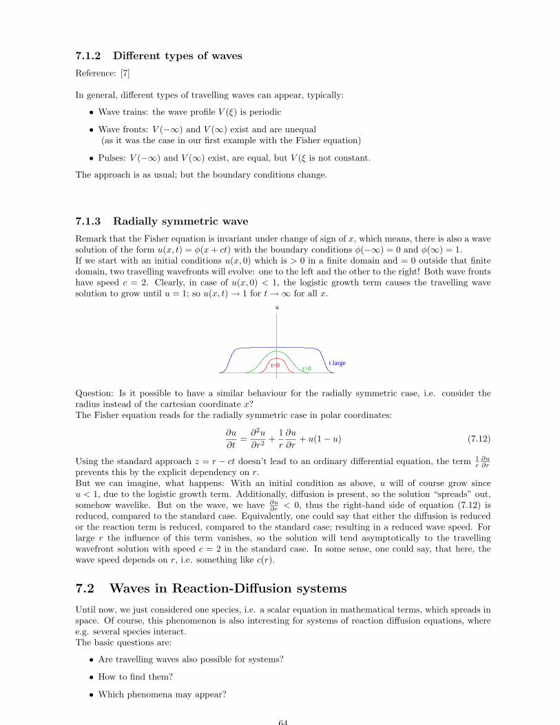
7.1.2 Different types of waves
Reference: [7]
In general, different types of travelling waves can appear, typically:
• Wave trains: the wave profile V (ξ) is periodic
• Wave fronts: V (−∞) and V (∞) exist and are unequal(as it was the case in our first example with the Fisher equation)
• Pulses: V (−∞) and V (∞) exist, are equal, but V (ξ is not constant.
The approach is as usual; but the boundary conditions change.
7.1.3 Radially symmetric wave
Remark that the Fisher equation is invariant under change of sign of x, which means, there is also a wavesolution of the form u(x, t) = φ(x + ct) with the boundary conditions φ(−∞) = 0 and φ(∞) = 1.If we start with an initial conditions u(x, 0) which is > 0 in a finite domain and = 0 outside that finitedomain, two travelling wavefronts will evolve: one to the left and the other to the right! Both wave frontshave speed c = 2. Clearly, in case of u(x, 0) < 1, the logistic growth term causes the travelling wavesolution to grow until u = 1; so u(x, t) → 1 for t → ∞ for all x.
u
t>0t=0 t large
Question: Is it possible to have a similar behaviour for the radially symmetric case, i.e. consider theradius instead of the cartesian coordinate x?The Fisher equation reads for the radially symmetric case in polar coordinates:
∂u
∂t=
∂2u
∂r2+
1
r
∂u
∂r+ u(1 − u) (7.12)
Using the standard approach z = r − ct doesn’t lead to an ordinary differential equation, the term 1r
∂u∂r
prevents this by the explicit dependency on r.But we can imagine, what happens: With an initial condition as above, u will of course grow sinceu < 1, due to the logistic growth term. Additionally, diffusion is present, so the solution “spreads” out,somehow wavelike. But on the wave, we have ∂u
∂r < 0, thus the right-hand side of equation (7.12) isreduced, compared to the standard case. Equivalently, one could say that either the diffusion is reducedor the reaction term is reduced, compared to the standard case; resulting in a reduced wave speed. Forlarge r the influence of this term vanishes, so the solution will tend asymptotically to the travellingwavefront solution with speed c = 2 in the standard case. In some sense, one could say, that here, thewave speed depends on r, i.e. something like c(r).
7.2 Waves in Reaction-Diffusion systems
Until now, we just considered one species, i.e. a scalar equation in mathematical terms, which spreads inspace. Of course, this phenomenon is also interesting for systems of reaction diffusion equations, wheree.g. several species interact.The basic questions are:
• Are travelling waves also possible for systems?
• How to find them?
• Which phenomena may appear?
64
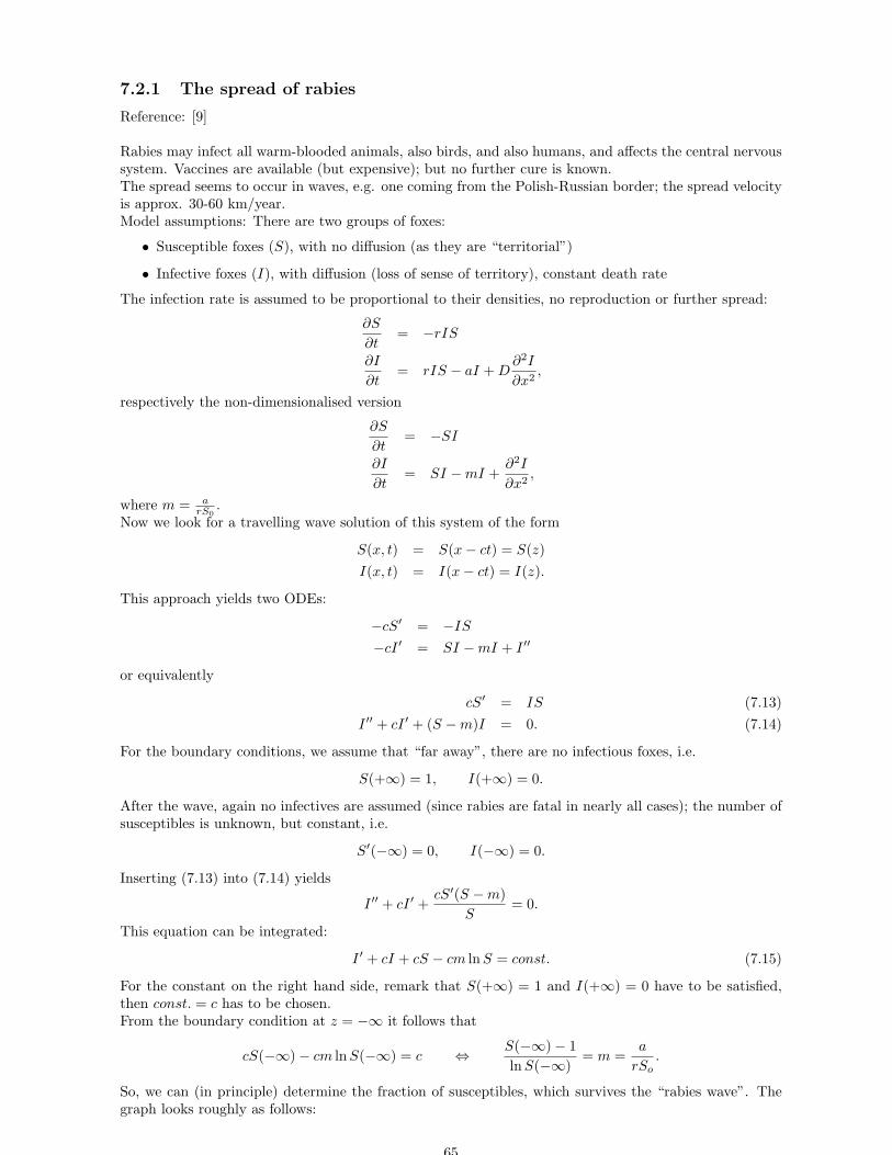
7.2.1 The spread of rabies
Reference: [9]
Rabies may infect all warm-blooded animals, also birds, and also humans, and affects the central nervoussystem. Vaccines are available (but expensive); but no further cure is known.The spread seems to occur in waves, e.g. one coming from the Polish-Russian border; the spread velocityis approx. 30-60 km/year.Model assumptions: There are two groups of foxes:
• Susceptible foxes (S), with no diffusion (as they are “territorial”)
• Infective foxes (I), with diffusion (loss of sense of territory), constant death rate
The infection rate is assumed to be proportional to their densities, no reproduction or further spread:
∂S
∂t= −rIS
∂I
∂t= rIS − aI + D
∂2I
∂x2,
respectively the non-dimensionalised version
∂S
∂t= −SI
∂I
∂t= SI − mI +
∂2I
∂x2,
where m = arS0
.Now we look for a travelling wave solution of this system of the form
S(x, t) = S(x − ct) = S(z)
I(x, t) = I(x − ct) = I(z).
This approach yields two ODEs:
−cS′ = −IS
−cI ′ = SI − mI + I ′′
or equivalently
cS′ = IS (7.13)
I ′′ + cI ′ + (S − m)I = 0. (7.14)
For the boundary conditions, we assume that “far away”, there are no infectious foxes, i.e.
S(+∞) = 1, I(+∞) = 0.
After the wave, again no infectives are assumed (since rabies are fatal in nearly all cases); the number ofsusceptibles is unknown, but constant, i.e.
S′(−∞) = 0, I(−∞) = 0.
Inserting (7.13) into (7.14) yields
I ′′ + cI ′ +cS′(S − m)
S= 0.
This equation can be integrated:
I ′ + cI + cS − cm ln S = const. (7.15)
For the constant on the right hand side, remark that S(+∞) = 1 and I(+∞) = 0 have to be satisfied,then const. = c has to be chosen.From the boundary condition at z = −∞ it follows that
cS(−∞) − cm lnS(−∞) = c ⇔ S(−∞) − 1
lnS(−∞)= m =
a
rSo.
So, we can (in principle) determine the fraction of susceptibles, which survives the “rabies wave”. Thegraph looks roughly as follows:
65
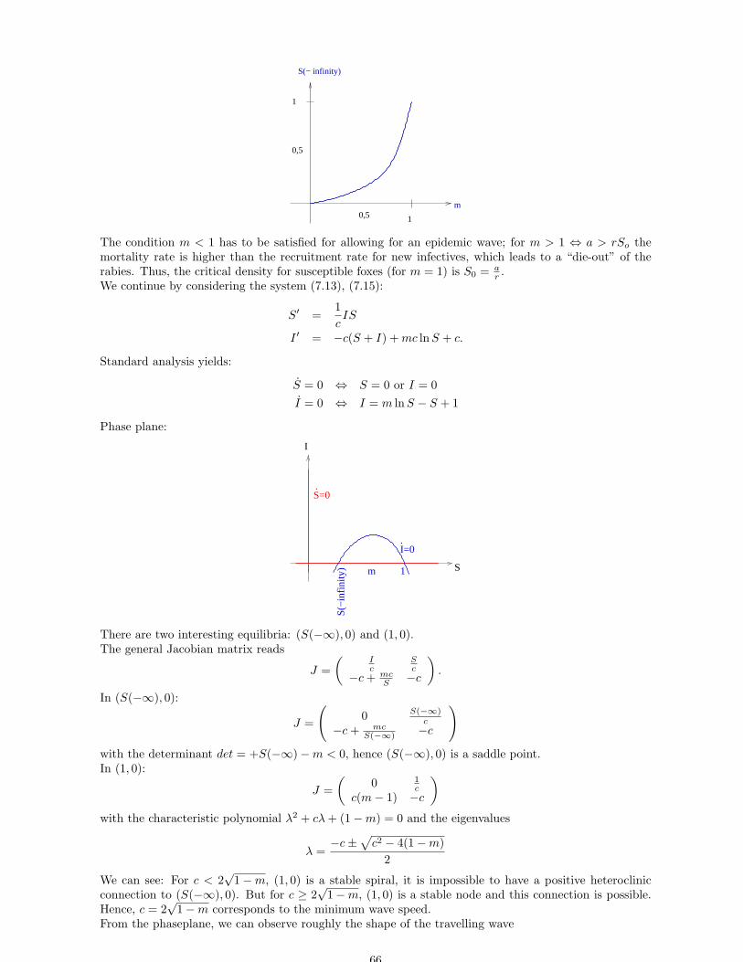
m
S(− infinity)
1
1
0,5
0,5
The condition m < 1 has to be satisfied for allowing for an epidemic wave; for m > 1 ⇔ a > rSo themortality rate is higher than the recruitment rate for new infectives, which leads to a “die-out” of therabies. Thus, the critical density for susceptible foxes (for m = 1) is S0 = a
r .We continue by considering the system (7.13), (7.15):
S′ =1
cIS
I ′ = −c(S + I) + mc lnS + c.
Standard analysis yields:
S = 0 ⇔ S = 0 or I = 0
I = 0 ⇔ I = m lnS − S + 1
Phase plane:
S
I
S=0.
I=0.
S(−
infin
ity) 1m
There are two interesting equilibria: (S(−∞), 0) and (1, 0).The general Jacobian matrix reads
J =
(Ic
Sc
−c + mcS −c
)
.
In (S(−∞), 0):
J =
(
0 S(−∞)c
−c + mcS(−∞) −c
)
with the determinant det = +S(−∞) − m < 0, hence (S(−∞), 0) is a saddle point.In (1, 0):
J =
(0 1
cc(m − 1) −c
)
with the characteristic polynomial λ2 + cλ + (1 − m) = 0 and the eigenvalues
λ =−c ±
√
c2 − 4(1 − m)
2
We can see: For c < 2√
1 − m, (1, 0) is a stable spiral, it is impossible to have a positive heteroclinicconnection to (S(−∞), 0). But for c ≥ 2
√1 − m, (1, 0) is a stable node and this connection is possible.
Hence, c = 2√
1 − m corresponds to the minimum wave speed.From the phaseplane, we can observe roughly the shape of the travelling wave
66
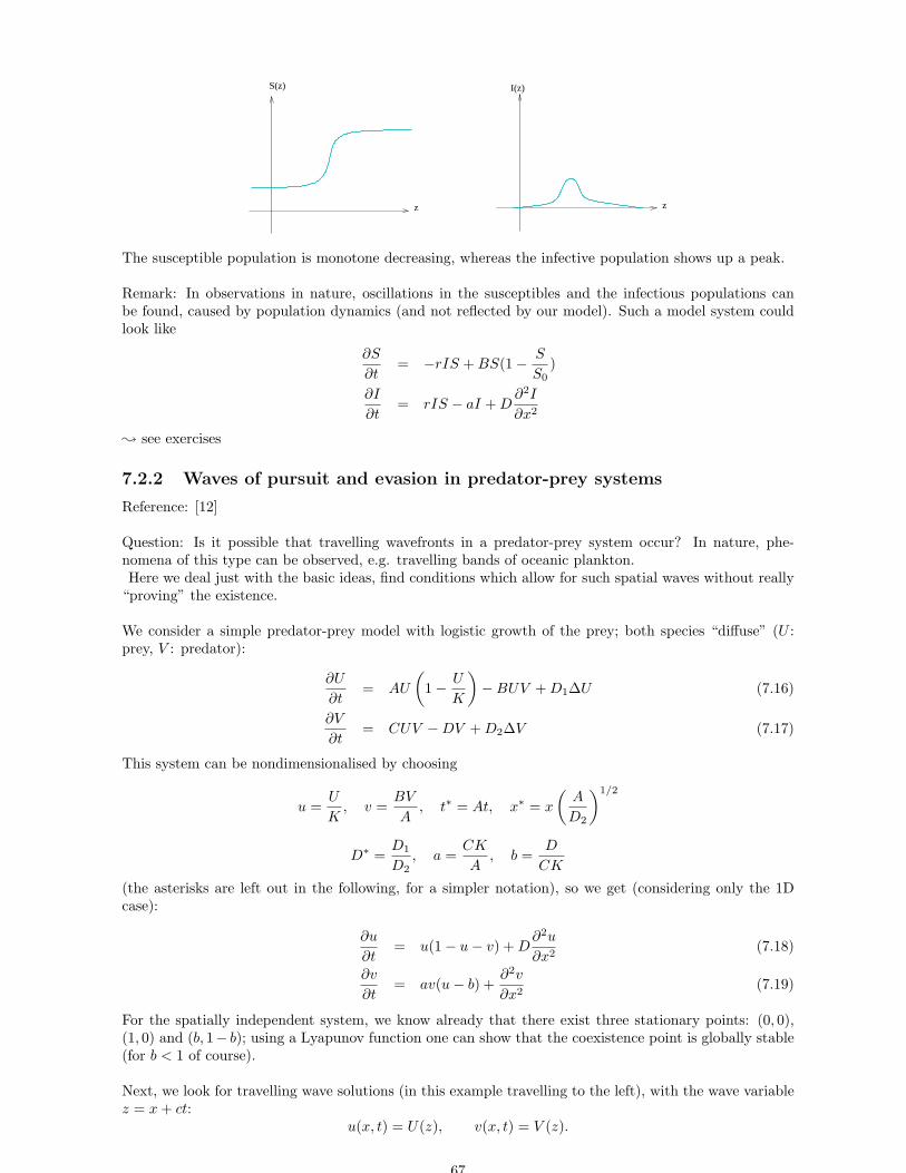
z z
S(z) I(z)
The susceptible population is monotone decreasing, whereas the infective population shows up a peak.
Remark: In observations in nature, oscillations in the susceptibles and the infectious populations canbe found, caused by population dynamics (and not reflected by our model). Such a model system couldlook like
∂S
∂t= −rIS + BS(1 − S
S0)
∂I
∂t= rIS − aI + D
∂2I
∂x2
; see exercises
7.2.2 Waves of pursuit and evasion in predator-prey systems
Reference: [12]
Question: Is it possible that travelling wavefronts in a predator-prey system occur? In nature, phe-nomena of this type can be observed, e.g. travelling bands of oceanic plankton.Here we deal just with the basic ideas, find conditions which allow for such spatial waves without really
“proving” the existence.
We consider a simple predator-prey model with logistic growth of the prey; both species “diffuse” (U :prey, V : predator):
∂U
∂t= AU
(
1 − U
K
)
− BUV + D1∆U (7.16)
∂V
∂t= CUV − DV + D2∆V (7.17)
This system can be nondimensionalised by choosing
u =U
K, v =
BV
A, t∗ = At, x∗ = x
(A
D2
)1/2
D∗ =D1
D2, a =
CK
A, b =
D
CK
(the asterisks are left out in the following, for a simpler notation), so we get (considering only the 1Dcase):
∂u
∂t= u(1 − u − v) + D
∂2u
∂x2(7.18)
∂v
∂t= av(u − b) +
∂2v
∂x2(7.19)
For the spatially independent system, we know already that there exist three stationary points: (0, 0),(1, 0) and (b, 1− b); using a Lyapunov function one can show that the coexistence point is globally stable(for b < 1 of course).
Next, we look for travelling wave solutions (in this example travelling to the left), with the wave variablez = x + ct:
u(x, t) = U(z), v(x, t) = V (z).
67
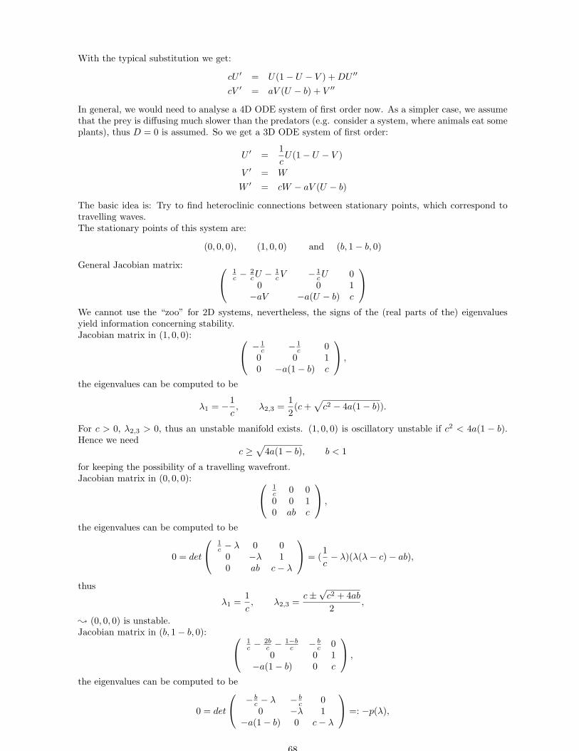
With the typical substitution we get:
cU ′ = U(1 − U − V ) + DU ′′
cV ′ = aV (U − b) + V ′′
In general, we would need to analyse a 4D ODE system of first order now. As a simpler case, we assumethat the prey is diffusing much slower than the predators (e.g. consider a system, where animals eat someplants), thus D = 0 is assumed. So we get a 3D ODE system of first order:
U ′ =1
cU(1 − U − V )
V ′ = W
W ′ = cW − aV (U − b)
The basic idea is: Try to find heteroclinic connections between stationary points, which correspond totravelling waves.The stationary points of this system are:
(0, 0, 0), (1, 0, 0) and (b, 1 − b, 0)
General Jacobian matrix:
1c − 2
cU − 1cV − 1
cU 00 0 1
−aV −a(U − b) c
We cannot use the “zoo” for 2D systems, nevertheless, the signs of the (real parts of the) eigenvaluesyield information concerning stability.Jacobian matrix in (1, 0, 0):
− 1c − 1
c 00 0 10 −a(1 − b) c
,
the eigenvalues can be computed to be
λ1 = −1
c, λ2,3 =
1
2(c +
√
c2 − 4a(1 − b)).
For c > 0, λ2,3 > 0, thus an unstable manifold exists. (1, 0, 0) is oscillatory unstable if c2 < 4a(1 − b).Hence we need
c ≥√
4a(1 − b), b < 1
for keeping the possibility of a travelling wavefront.Jacobian matrix in (0, 0, 0):
1c 0 00 0 10 ab c
,
the eigenvalues can be computed to be
0 = det
1c − λ 0 0
0 −λ 10 ab c − λ
= (1
c− λ)(λ(λ − c) − ab),
thus
λ1 =1
c, λ2,3 =
c ±√
c2 + 4ab
2,
; (0, 0, 0) is unstable.Jacobian matrix in (b, 1 − b, 0):
1c − 2b
c − 1−bc − b
c 00 0 1
−a(1 − b) 0 c
,
the eigenvalues can be computed to be
0 = det
− bc − λ − b
c 00 −λ 1
−a(1 − b) 0 c − λ
=: −p(λ),
68
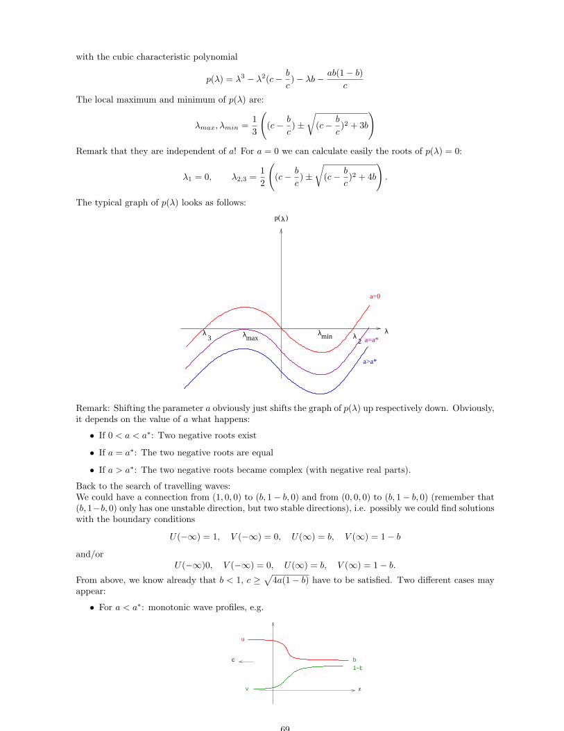
with the cubic characteristic polynomial
p(λ) = λ3 − λ2(c − b
c) − λb − ab(1 − b)
c
The local maximum and minimum of p(λ) are:
λmax, λmin =1
3
(
(c − b
c) ±
√
(c − b
c)2 + 3b
)
Remark that they are independent of a! For a = 0 we can calculate easily the roots of p(λ) = 0:
λ1 = 0, λ2,3 =1
2
(
(c − b
c) ±
√
(c − b
c)2 + 4b
)
.
The typical graph of p(λ) looks as follows:
λ
p( )λ
λ
a=0
λminλmaxλ
3 2 a=a*
a>a*
Remark: Shifting the parameter a obviously just shifts the graph of p(λ) up respectively down. Obviously,it depends on the value of a what happens:
• If 0 < a < a∗: Two negative roots exist
• If a = a∗: The two negative roots are equal
• If a > a∗: The two negative roots became complex (with negative real parts).
Back to the search of travelling waves:We could have a connection from (1, 0, 0) to (b, 1− b, 0) and from (0, 0, 0) to (b, 1− b, 0) (remember that(b, 1−b, 0) only has one unstable direction, but two stable directions), i.e. possibly we could find solutionswith the boundary conditions
U(−∞) = 1, V (−∞) = 0, U(∞) = b, V (∞) = 1 − b
and/orU(−∞)0, V (−∞) = 0, U(∞) = b, V (∞) = 1 − b.
From above, we know already that b < 1, c ≥√
4a(1 − b) have to be satisfied. Two different cases mayappear:
• For a < a∗: monotonic wave profiles, e.g.
z
1−bb
v
u
c
69
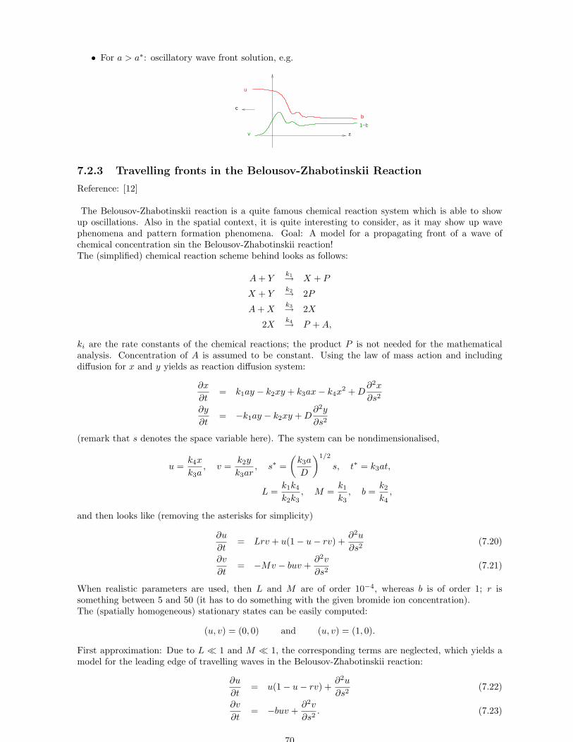
• For a > a∗: oscillatory wave front solution, e.g.
zv
u
c
b
1−b
7.2.3 Travelling fronts in the Belousov-Zhabotinskii Reaction
Reference: [12]
The Belousov-Zhabotinskii reaction is a quite famous chemical reaction system which is able to showup oscillations. Also in the spatial context, it is quite interesting to consider, as it may show up wavephenomena and pattern formation phenomena. Goal: A model for a propagating front of a wave ofchemical concentration sin the Belousov-Zhabotinskii reaction!The (simplified) chemical reaction scheme behind looks as follows:
A + Yk1→ X + P
X + Yk2→ 2P
A + Xk3→ 2X
2Xk4→ P + A,
ki are the rate constants of the chemical reactions; the product P is not needed for the mathematicalanalysis. Concentration of A is assumed to be constant. Using the law of mass action and includingdiffusion for x and y yields as reaction diffusion system:
∂x
∂t= k1ay − k2xy + k3ax − k4x
2 + D∂2x
∂s2
∂y
∂t= −k1ay − k2xy + D
∂2y
∂s2
(remark that s denotes the space variable here). The system can be nondimensionalised,
u =k4x
k3a, v =
k2y
k3ar, s∗ =
(k3a
D
)1/2
s, t∗ = k3at,
L =k1k4
k2k3, M =
k1
k3, b =
k2
k4,
and then looks like (removing the asterisks for simplicity)
∂u
∂t= Lrv + u(1 − u − rv) +
∂2u
∂s2(7.20)
∂v
∂t= −Mv − buv +
∂2v
∂s2(7.21)
When realistic parameters are used, then L and M are of order 10−4, whereas b is of order 1; r issomething between 5 and 50 (it has to do something with the given bromide ion concentration).The (spatially homogeneous) stationary states can be easily computed:
(u, v) = (0, 0) and (u, v) = (1, 0).
First approximation: Due to L ≪ 1 and M ≪ 1, the corresponding terms are neglected, which yields amodel for the leading edge of travelling waves in the Belousov-Zhabotinskii reaction:
∂u
∂t= u(1 − u − rv) +
∂2u
∂s2(7.22)
∂v
∂t= −buv +
∂2v
∂s2. (7.23)
70
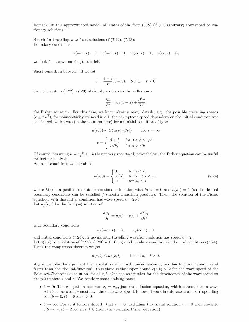
Remark: In this approximated model, all states of the form (0, S) (S > 0 arbitrary) correspond to sta-tionary solutions.
Search for travelling wavefront solutions of (7.22), (7.23):Boundary conditions:
u(−∞, t) = 0, v(−∞, t) = 1, u(∞, t) = 1, v(∞, t) = 0,
we look for a wave moving to the left.
Short remark in between: If we set
v =1 − b
r(1 − u), b 6= 1, r 6= 0,
then the system (7.22), (7.23) obviously reduces to the well-known
∂u
∂t= bu(1 − u) +
∂2u
∂s2,
the Fisher equation. For this case, we know already many details; e.g. the possible travelling speeds(c ≥ 2
√b), for nonnegativity we need b < 1; the asymptotic speed dependent on the initial condition was
considered, which was (in the notation here) for an initial condition of type
u(s, 0) ∼ O(exp(−βs)) for s → ∞
c =
β + bβ for 0 < β ≤
√b
2√
b, for β >√
b
Of course, assuming v = 1−br (1−u) is not very realistical; nevertheless, the Fisher equation can be useful
for further analysis.As intial conditions we introduce
u(s, 0) =
0 for s < s1
h(s) for s1 < s < s2
1 for s2 < s,(7.24)
where h(s) is a positive monotonic continuous function with h(s1) = 0 and h(s2) = 1 (so the desiredboundary conditions can be satisfied / smooth transition possible). Then, the solution of the Fisherequation with this initial condition has wave speed c = 2
√b.
Let uf (s, t) be the (unique) solution of
∂uf
∂t= uf (1 − uf ) +
∂2uf
∂s2
with boundary conditionsuf (−∞, t) = 0, uf (∞, t) = 1
and initial conditions (7.24); its asymptotic travelling wavefront solution has speed c = 2.Let u(s, t) be a solution of (7.22), (7.23) with the given boundary conditions and initial conditions (7.24).Using the comparison theorem we get
u(s, t) ≤ uf (s, t) for all s, t > 0.
Again, we take the argument that a solution which is bounded above by another function cannot travelfaster than the “bound-function”, thus there is the upper bound c(r, b) ≤ 2 for the wave speed of theBelousov-Zhabotinskii solution, for all r, b. One can ask further for the dependency of the wave speed onthe parameters b and r. We consider some limiting cases:
• b = 0: The v equation becomes vt = vss, just the diffusion equation, which cannot have a wavesolution. As u and v must have the same wave speed, it doesn’t work in this case at all, correspondingto c(b → 0, r) = 0 for r > 0.
• b → ∞: For v, it follows directly that v = 0; excluding the trivial solution u = 0 then leads toc(b → ∞, r) = 2 for all r ≥ 0 (from the standard Fisher equation)
71
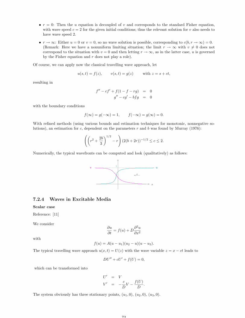
• r = 0: Then the u equation is decoupled of v and corresponds to the standard Fisher equation,with wave speed c = 2 for the given initial conditions; thus the relevant solution for v also needs tohave wave speed 2.
• r → ∞: Either u = 0 or v = 0, so no wave solution is possible, corresponding to c(b, r → ∞) = 0.(Remark: Here we have a nonuniform limiting situation; the limit r → ∞ with v 6= 0 does notcorrespond to the situation with v = 0 and then letting r → ∞, as in the latter case, u is governedby the Fisher equation and r does not play a role).
Of course, we can apply now the classical travelling wave approach, let
u(s, t) = f(z), v(s, t) = g(z) with z = s + ct,
resulting in
f ′′ − cf ′ + f(1 − f − rg) = 0
g′′ − cg′ − bfg = 0
with the boundary conditions
f(∞) = g(−∞) = 1, f(−∞) = g(∞) = 0.
With refined methods (using various bounds and estimation techniques for monotonic, nonnegative so-lutions), an estimation for c, dependent on the parameters r and b was found by Murray (1976):
((
r2 +2b
3
)1/2
− r
)
(2(b + 2r))−1/2 ≤ c ≤ 2.
Numerically, the typical wavefronts can be computed and look (qualitatively) as follows:
z
v 1 u
c
7.2.4 Waves in Excitable Media
Scalar case
Reference: [11]
We consider∂u
∂t= f(u) + D
∂2u
∂x2
withf(u) = A(u − u1)(u2 − u)(u − u3).
The typical travelling wave approach u(x, t) = U(z) with the wave variable z = x − ct leads to
DU ′′ + cU ′ + f(U) = 0,
which can be transformed into
U ′ = V
V ′ = − c
DV − f(U)
D.
The system obviously has three stationary points, (u1, 0), (u2, 0), (u3, 0).
72
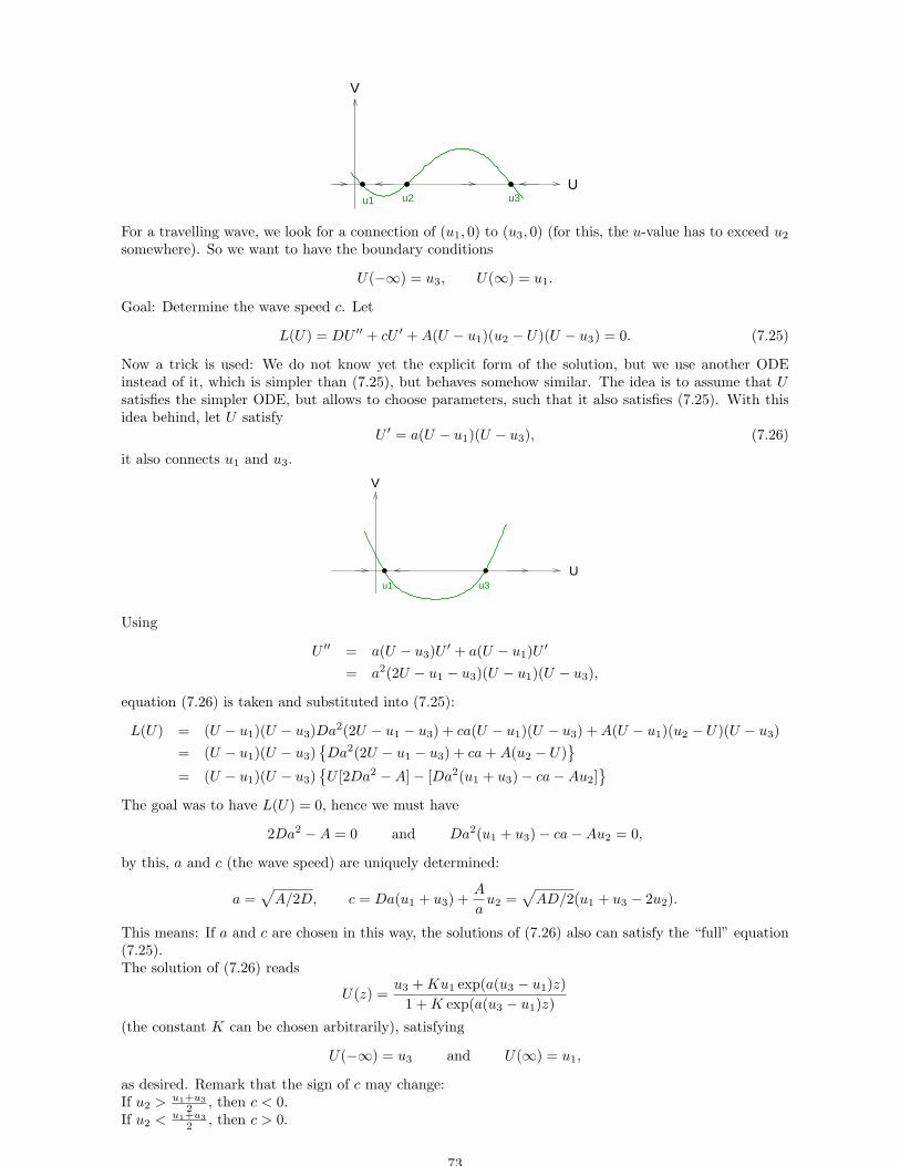
U
V
u1 u2 u3
For a travelling wave, we look for a connection of (u1, 0) to (u3, 0) (for this, the u-value has to exceed u2
somewhere). So we want to have the boundary conditions
U(−∞) = u3, U(∞) = u1.
Goal: Determine the wave speed c. Let
L(U) = DU ′′ + cU ′ + A(U − u1)(u2 − U)(U − u3) = 0. (7.25)
Now a trick is used: We do not know yet the explicit form of the solution, but we use another ODEinstead of it, which is simpler than (7.25), but behaves somehow similar. The idea is to assume that Usatisfies the simpler ODE, but allows to choose parameters, such that it also satisfies (7.25). With thisidea behind, let U satisfy
U ′ = a(U − u1)(U − u3), (7.26)
it also connects u1 and u3.
U
V
u1 u3
Using
U ′′ = a(U − u3)U′ + a(U − u1)U
′
= a2(2U − u1 − u3)(U − u1)(U − u3),
equation (7.26) is taken and substituted into (7.25):
L(U) = (U − u1)(U − u3)Da2(2U − u1 − u3) + ca(U − u1)(U − u3) + A(U − u1)(u2 − U)(U − u3)
= (U − u1)(U − u3)Da2(2U − u1 − u3) + ca + A(u2 − U)
= (U − u1)(U − u3)U [2Da2 − A] − [Da2(u1 + u3) − ca − Au2]
The goal was to have L(U) = 0, hence we must have
2Da2 − A = 0 and Da2(u1 + u3) − ca − Au2 = 0,
by this, a and c (the wave speed) are uniquely determined:
a =√
A/2D, c = Da(u1 + u3) +A
au2 =
√
AD/2(u1 + u3 − 2u2).
This means: If a and c are chosen in this way, the solutions of (7.26) also can satisfy the “full” equation(7.25).The solution of (7.26) reads
U(z) =u3 + Ku1 exp(a(u3 − u1)z)
1 + K exp(a(u3 − u1)z)
(the constant K can be chosen arbitrarily), satisfying
U(−∞) = u3 and U(∞) = u1,
as desired. Remark that the sign of c may change:If u2 > u1+u3
2 , then c < 0.If u2 < u1+u3
2 , then c > 0.
73
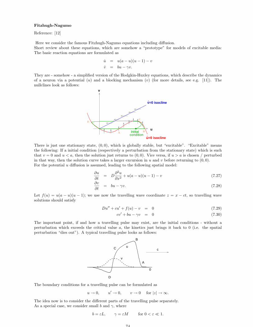
Fitzhugh-Nagumo
Reference: [12]
Here we consider the famous Fitzhugh-Nagumo equations including diffusion.Short review about these equations, which are somehow a “prototype” for models of excitable media:The basic reaction equations are formulated as
u = u(a − u)(u − 1) − v
v = bu − γv.
They are - somehow - a simplified version of the Hodgkin-Huxley equations, which describe the dynamicsof a neuron via a potential (u) and a blocking mechanism (v) (for more details, see e.g. [11]). Thenullclines look as follows:
u
v
v=0 isocline.
u=0 isocline.
Initialcondition
A B
CD
There is just one stationary state, (0, 0), which is globally stable, but “excitable”. “Excitable” meansthe following: If a initial condition (respectively a perturbation from the stationary state) which is suchthat v = 0 and u < a, then the solution just returns to (0, 0). Vice versa, if u > a is chosen / perturbedin that way, then the solution curve takes a larger excursion in u and v before returning to (0, 0).For the potential u diffusion is assumed, leading to the following spatial model:
∂u
∂t= D
∂2u
∂x2+ u(a − u)(u − 1) − v (7.27)
∂v
∂t= bu − γv. (7.28)
Let f(u) = u(a − u)(u − 1); we use now the travelling wave coordinate z = x − ct, so travelling wavesolutions should satisfy
Du′′ + cu′ + f(u) − v = 0 (7.29)
cv′ + bu − γv = 0 (7.30)
The important point, if and how a travelling pulse may exist, are the initial conditions - without aperturbation which exceeds the critical value a, the kinetics just brings it back to 0 (i.e. the spatialperturbation “dies out”). A typical travelling pulse looks as follows:
0
A
B
C
D
cu
v
The boundary conditions for a travelling pulse can be formulated as
u → 0, u′ → 0, v → 0 for |z| → ∞.
The idea now is to consider the different parts of the travelling pulse separately.As a special case, we consider small b and γ, where
b = εL, γ = εM for 0 < ε ≪ 1.
74
Then our system reads
ut = Duxx + f(u) − v
vt = ε(Lu − Mv).
If we consider the leading front of the wave pulse (0AB), then for ε → 0 we have v ≈ const. = 0, i.e. thesystem collapses to
ut = Duxx + f(u),
where f(u) = u(a − u)(u − 1). From the scalar excitable system above, we get immediately the wavespeed:
c =
(D
2
)1/2
(1 − 2a).
This is only positive, if a < 12 .
Next we consider the part BC; obviously there v changes - due to vt = O(ε) this takes a long time (O( 1ε )).
This can be done by a singular perturbation analysis (left out here).The next question arises: Where is C positioned on the phase trajectory? For this, it is important toremark that the wave speed of this so-called “trailing edge” has to be the same as for 0AB, as they haveto form one wave pulse. Due to the fast time scale, v doesn’t change (much), so we have on this part onthe trajectory approximately v ≈ vC and we get the equation
ut = Duxx + f(u) − vC
For the boundary conditions we need
u(−∞) = uD, u(∞) = uC .
Let uC , uD and uP be the roots of f(u) = vC , then we can use again the scalar example to get aninformation about the wave speed:
c =
√
D
2(uC − 2uP + uD).
If we express uC , uD and uP in terms of vC , then c(vC) is a function of vC . Hence, as the wave speedhas to be the same as for 0AB, c is fixed and by that vC can be uniquely determined (it is a polynomialwhich has to be solved).As a last step, one could consider the part D0, called the “refractory phase”. This is again a slow process,we leave it out now.
Such threshold waves are also obtained in many other examples, e.g. two-species systems where oneof the reactions is fast.
Poincare inequality
Reference: [7]
Often, one considers an ODE of the following form:
d2y
dx2+ λy = 0
with the boundary conditionsdy(0)
dx=
dy(1)
dx= 0.
So, we get an “eigenvalue problem” with the eigensolutions
φn(x) = cos nπx, n = 0, 1, 2
with λ = λn = n2π2. For any function w(x) which satisfies the boundary conditions and is twicedifferentiable, the second derivative can be written as
d2w
dx2=
∞∑
n=0
an cos nπx (7.31)
75
with the coefficients
a0 =
∫ 1
0
d2w
dx2dx =
[dw
dx
]1
0
= 0
an = 2
∫ 1
0
d2w
dx2cos nπx dx for n ≥ 1.
We take (7.31) and integrate it twice, with respect to the boundary condition, thus we get
w(x) =
∞∑
n=0
− an
n2π2cos nπx + C
Remark that ∫ 1
0
cos(kπx) · cos(lπx) dx =
0 for k 6= l12 for k = l
Furthermore we find:
∫ 1
0
(dw
dx
)2
dx =
[
wdw
dx
]1
0︸ ︷︷ ︸
=0
−∫ 1
0
wd2w
dx2dx
=
∫ 1
0
( ∞∑
n=0
an
n2π2cos nπx
) ( ∞∑
n=0
an cos nπx
)
dx − C
∫ 1
0
( ∞∑
n=0
an cos nπx
)
dx
︸ ︷︷ ︸
=0
=1
2
∞∑
n=0
a2n
n2π2
≤ 1
2π2
∞∑
n=0
a2n (7.32)
and (by taking (7.31), multiplying it by d2wdx2 and integrating)
∫ 1
0
(d2w
dx2
)2
dx =∞∑
n=0
an
∫ 1
0
d2w
dx2cos nπx dx =
1
2
∞∑
n=0
a2n
(this is the Parseval equality!)We insert this Parseval equality into (7.32) and get
∫ 1
0
(dw
dx
)2
dx ≤ 1
π2
∫ 1
0
(d2w
dx2
)
dx, (7.33)
which is called the “Poincare inequality”.
Criteria for a pulse
Reference: [7]
We can consider in greater detail the conditions how the threshold has to be exceeded to cause re-ally a peak, or - vice versa - which conditions still just lead to a decay effect. For that purpose weconsider the Fitzhugh-Nagumo equations (7.27), (7.28) with the following conditions for a stimulus atx = 0 which act over a finite time interval:
u(0, t) = P (t) u(x, 0) = 0 (7.34)
v(0, t) = b
∫ t
0
P (s)e−γsds v(x, 0) = 0 (7.35)
and, as the stimulus only should at during a finite time interval, P (t) = 0 for t ≥ T .Further assumptions: u(x, t), v(x, t) tend to 0 for x → ∞, such that
∫ ∞0
u2(x, t) dx,∫ ∞0
v2(x, t) dx exist
76
and are finite for all t. For simplicity, we assume D = 1 in the following.Next, (7.27) is multiplied by bu and (7.28) is multiplied by v; subtracting the resulting equations yields
bu∂2u
∂x2− v
∂v
∂t= bu
∂u
∂t− bu2(1 − u)(u − a) + buv − buv − γv2
⇔ bu∂u
∂t+ v
∂v
∂t= bu
∂2u
∂x2+ bu2(1 − u)(u − a) − γv2
⇔ 1
2
∂
∂t(bu2 + v2) = b
∂
∂x(u
∂u
∂x) − b(
∂u
∂x)2 + bu2(1 − u)(u − a) − γv2
This equation is integrated over x (apply the initial condition (7.34), then it follows for t ≥ T :
1
2
d
dt
∫ ∞
0
(bu2 + v2) dx =
∫ ∞
0
b∂
∂x(u
∂u
∂x) dx
︸ ︷︷ ︸
=0
−b
∫ ∞
0
(∂u
∂x
2
dx +
∫ ∞
0
(bu2(1 − u)(u − a) − γv2) dv
≤∫ ∞
0
(bu2(1 − u)(u − a) − γv2) dx
Let u(x, t) < a for all x, t > 0, then the following estimate can be used for a constant δ (δ depends on a):
u2(1 − u)(u − a) ≤ −δu2.
If we use this above, we get
1
2
d
dt
∫ ∞
0
(bu2 + v2) dx ≤ −∫ ∞
0
(bδu2 + γv2) dx.
Let C = minδ, γ, then it can be rewritten as
d
dt
∫ ∞
0
(bu2 + v2) dx ≤ −2C
∫ ∞
0
(bu2 + v2) dx,
which yields in the end the estimate
∫ ∞
0
(bu2 + v2) dx ≤ Ke−2Ct.
The result is: Starting with an action potential below the potential value a leads to an exponential decayin time for the mean square of u(x, t). One can show a more precise statement (without proof here):Let a > b
γ and P (t) bounded, continuous and satisfying the conditions
(i) P (t) = P (0) = 0 for all t ≥ T > 0
(ii) supt≥0 |P (t)| ≤ M .
Then
supx≥0
|u(x, t)| ≤ k
∫ t
0
|P (s)| ds for all t ≥ T
and there are constants C, k, λ such that if∫ T
0|P | dt < λ, then
supx≥0
|u(x, t)| ≤ k exp(−Ct), t ≥ 0.
Also possible to show: If M is sufficiently small, then
supx≥0
|u(x, t)| ≤ k exp(−Ct), t ≥ 0.
Now we consider a more realistic problem with finitely long nerves (length l). At x = 0 we start againwith
u(0, t) = P (t)
v(0, t) = b
∫ t
0
P (s)e−γs ds.
77
At x = l, one could assume either a Dirichlet condition
u(l, t) = 0 for t ≥ 0
or Robin condition∂u(l, t)
dx− αu(l, t) = 0, for t ≥ 0, α ≤ 0
For P (t) we assume that P (t) = 0 for t ≥ T .(7.27) is multiplied by u, (7.28) is multiplied by b−1v, subtracting yields
1
2
∂
∂t(u2 +
v2
b) = u
∂2u
∂x2+ u2(1 − u)(u − a) − γ
bv2,
integrating yields
1
2
∫ l
0
∂
∂t(u2 +
v2
b) dx =
∫ l
0
(u∂2u
∂x2+ u2(1 − u)(u − a) − γ
bv2) dx.
Remark that∫ l
0
u∂2u
∂x2dx =
[
u∂u
∂x
]l
0
−∫ l
0
(∂u
∂x
)2
dx,
taking into account the boundary condition u(0, t) = 0 = u(l, t), t ≥ T , results in
∫ l
0
u∂2u
∂x2dx = −
∫ l
0
(∂u
∂x
)2
dx.
Analogously, for the Robin condition u(0, t) = 0 = ∂∂xu(l, t) − αu(l, t), t ≥ T , we find
∫ l
0
u∂2u
∂x2dx =
[
u∂u
∂x
]l
0︸ ︷︷ ︸
=αu2(l,t)
−∫ l
0
(∂u
∂x)2 dx ≤ −
∫ l
0
(∂u
∂x)2 dx
due to α ≤ 0.For both cases we get
1
2
∂
∂t
∫ l
0
(u2 +v2
b) dx ≤
∫ l
0
(u2(1 − u)(u − a) − γ
bv2) dx −
∫ l
0
(∂u
∂x)2 dx.
Remark that the term (1 − u)(u − 1) has a maximum at u = (1−a)2 and assumes there the value (1−a)2
4 ,so we can use this estimate and get
1
2
∂
∂t
∫ l
0
(u2 +v2
b) dx ≤
∫ l
0
((1 − a)2
4u2 − γ
bv2 − (
∂u
∂x)2
)
dx.
For the Dirichlet boundary conditions u(0, t) = 0 = u(l, t), t ≥ T , we can directly apply the Poincareinequality (7.33), which reads in our case
∫ l
0
(∂u
∂x)2 dx ≥ (
π
l)2
∫ l
0
u2 dx
Remark that the conditions for the Poincare inequality are satisfied by using u = dwdt . This also works in
a similar way for the Robin boundary condition at x = l.So we get
1
2
∂
∂t
∫ l
0
(u2 +v2
b) dx ≤
∫ l
0
(
((1 − a)2
4− π2
l2)u2 − γ
bv2
)
dx.
Considering that case with l < 2π(1−a) ⇔ (1−a)2
4 − π2
l2 < 0, one can formulate
∂
∂t
∫ l
0
(u2 +v2
b) dx ≤ −2C
∫ l
0
(u2 +v2
b) dx,
78
where C is chosen as
C = max
π2
l2− (1 − a)2
4, γ
.
Using this formulation, it follows again, that
∫ l
0
(u2 +v2
b) dx
decays exponentially.What does this mean from a biological point of view? If l (the length of the axon) is not sufficientlylong, then all stimuli decay exponentially in time. Nevertheless, also an infinitely long axon may notpropagate a stimulus, but it is not completely clear until now, how P (t) really has to look like, such thata propagation of an action potential is possible.
For some more details concerning the influence of the axon length on the behaviour of possible solu-tions, see e.g. [2]
7.2.5 Travelling Wave Trains in Reaction Diffusion Systems with OscillatoryKinetics
Reference: [12]
In this subsection, we consider reaction diffusion systems with reaction terms that possess limit cycles;one can expect wavetrain solutions when including diffusion. In general such systems look like
∂u
∂t= f(u) +
∂2u
∂x2(7.36)
For the reaction term, i.e. the spatially homogeneous system, we assume a dependency on a parameter(which is used as bifurcation parameter later), so
du
dt= f(u, γ).
For γ < γc it is assumed to possess a stable stationary state, and a Hopf bifurcation appears at γ = γc,such that the stationary state looses its stability and a stable limit cycle solutions appears (at least forγ = γc + ε where 0 < ε ≪ 1).Now we look for a travelling plane wavetrain solution, thus we use the approach
u(x, t) = U(z), z = σt − kx,
where U is a 2π-periodic function of z, the so-called “phase”. (Remark that this is just a slight gen-eralisation of the former approach, using the frequency σ > 0 and the wavenumber k; resulting in thewavelength ω = 2π/k and the wavespeed c = σ/k). We insert this approach into (7.36): and get thefollowing ODE system:
k2U ′′ − σU ′ + f(U) = 0
How to choose σ and k such that this equation has a 2π periodic solution U?As a special case, we consider the so-called λ − ω system as a prototype for such a system. It includestwo reactants u and v and reads
∂
∂t
(uv
)
=
(λ(r) −ω(r)ω(r) λ(r)
)(uv
)
+∂2
∂x2
(uv
)
, (7.37)
where r2 = u2 + v2; λ(r) and ω(r) are real functions of r. For guaranteeing the limit cycle solution, weneed an isolated zero r0 > 0 of λ(r), λ′(r0) < 0 and ω(r0) 6= 0.Next we change the used variables (u, v) into polar coordinates (r, θ), via
u = r cos θ, v = r sin θ. (7.38)
The transformed system becomes
rt = rλ(r) + rxx − rθ2x (7.39)
θt = ω(r) +1
r2(r2θx)x. (7.40)
79
If the isolated zero r0 > 0 of λ(r) exists and the condition λ′(r0) is also satisfied, then we can seeimmediately the limit cycle solution of the kinetics:
r = r0 and θ = θ0 + ω(r0)t.
(θ0 is an arbitrary phase). Retransforming this result via (7.38) yields the limit cycle solution in theoriginal variables u and v:
u = r0 cos(ω(r0)t + θ0), v = r0 sin(ω(r0)t + θ0),
they also have frequency ω(r0) and amplitude r0.
If we now look for a travelling plane wave solution as introduced above, i.e. u(x, t) = U(z), v(x, t) = V (t)and z = σt − kx, then they read in the polar form
r = α, θ = σt − kx,
due to the claim that U , V are periodic (sin, cos with period 2π (thus the radius has to be constant andθ shows the desired behaviour). (Remark: Then u = r cos θ and v = r sin θ are periodic as desired)Inserting this approach into (7.39) yields
0 = αλ(α) − αk2
σ = ω(α) +1
α2(α2(−k))x,
thusσ = ω(α) and k2 = λ(α). (7.41)
Using α as the “relevant” parameter yields a one-parameter family of travelling wave train solutions ofthe two-reactants model which can be written as
u = α cos(ω(αt − xλ1/2(α))
v = α sin(ω(α)t − xλ1/2(α)).
The corresponding wave speed is
c =σ
k=
ω(α)
λ1/2(α).
Letting r = α tend to r0 with the conditions from above, this means that there is the limit cycle solution,where λ(r) → 0 by definition; correspondingly k → 0 (k was the wave number).
We consider an example:ω(r) = 1, λ(r) = γ − r2
The reaction dynamics,
∂u
∂t= λ(r)u − ω(r)v = (γ − (u2 + v2))u − v
∂v
∂t= ω(r)u + λ(r)v = u + (γ − (u2 + v2))v,
has a stationary point at (u, v) = (0, 0).The Jacobian matrix reads (
γ − 3u2 − v2 −11 γ − u2 − 3v2
)
,
i.e. in (0, 0):
(γ −11 γ
)
, the characteristic polynomial reads (γ − λ)2 + 1 = 0, thus
λ2 − 2γλ + γ2 + 1 = 0 ⇔ λ1,2 =2γ ±
√
4γ2 − 4(γ2 + 1)
2= γ ± i.
Hence, obviously (0, 0) is stable for γ < 0 and unstable for γ > 0. Using γ as bifurcation parameter forγc = 0, the eigenvalues are ±i, satisfying the standard Hopf bifurcation requirement. Thus, for γ = γc +ε
80
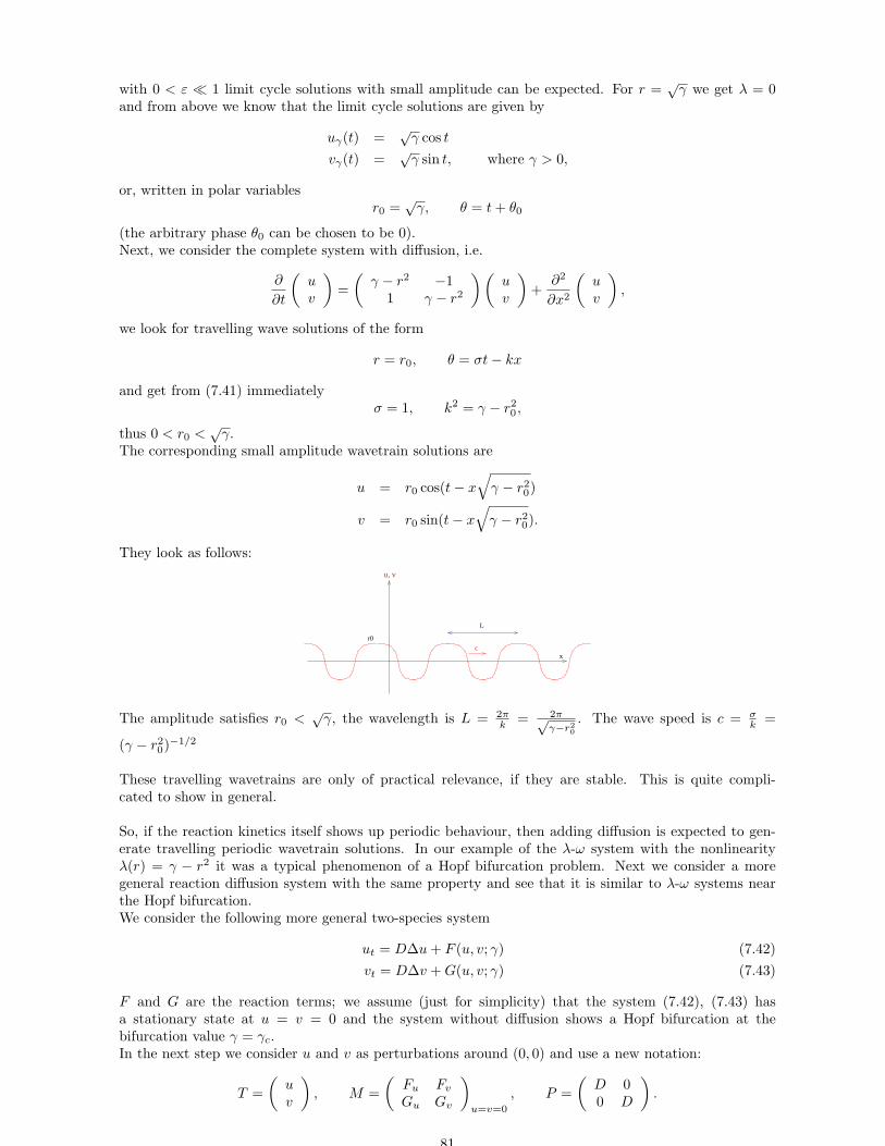
with 0 < ε ≪ 1 limit cycle solutions with small amplitude can be expected. For r =√
γ we get λ = 0and from above we know that the limit cycle solutions are given by
uγ(t) =√
γ cos t
vγ(t) =√
γ sin t, where γ > 0,
or, written in polar variablesr0 =
√γ, θ = t + θ0
(the arbitrary phase θ0 can be chosen to be 0).Next, we consider the complete system with diffusion, i.e.
∂
∂t
(uv
)
=
(γ − r2 −1
1 γ − r2
)(uv
)
+∂2
∂x2
(uv
)
,
we look for travelling wave solutions of the form
r = r0, θ = σt − kx
and get from (7.41) immediatelyσ = 1, k2 = γ − r2
0,
thus 0 < r0 <√
γ.The corresponding small amplitude wavetrain solutions are
u = r0 cos(t − x√
γ − r20)
v = r0 sin(t − x√
γ − r20).
They look as follows:
u, v
L
cx
r0
The amplitude satisfies r0 <√
γ, the wavelength is L = 2πk = 2π√
γ−r20
. The wave speed is c = σk =
(γ − r20)
−1/2
These travelling wavetrains are only of practical relevance, if they are stable. This is quite compli-cated to show in general.
So, if the reaction kinetics itself shows up periodic behaviour, then adding diffusion is expected to gen-erate travelling periodic wavetrain solutions. In our example of the λ-ω system with the nonlinearityλ(r) = γ − r2 it was a typical phenomenon of a Hopf bifurcation problem. Next we consider a moregeneral reaction diffusion system with the same property and see that it is similar to λ-ω systems nearthe Hopf bifurcation.We consider the following more general two-species system
ut = D∆u + F (u, v; γ) (7.42)
vt = D∆v + G(u, v; γ) (7.43)
F and G are the reaction terms; we assume (just for simplicity) that the system (7.42), (7.43) hasa stationary state at u = v = 0 and the system without diffusion shows a Hopf bifurcation at thebifurcation value γ = γc.In the next step we consider u and v as perturbations around (0, 0) and use a new notation:
T =
(uv
)
, M =
(Fu Fv
Gu Gv
)
u=v=0
, P =
(D 00 D
)
.
81
Using this notation we can write the full system as
Tt = MT + P∆T + H, where H =
(f(u, v; γ)g(u, v; γ)
)
,
then f and g denote the nonlinear contribution of F and G to u and v near u = v = 0; or the linearisedform is
Tt = MT + P∆T.
According to the assumption, the kinetics has a Hopf bifurcation at γ = γc. This means, in the newnotation, that the eigenvalues of the matrix M (denoted by σ) have the property that
Reσ(γ) < 0 for γ < γc
Reσ(γc) = 0, Imσ(γc) 6= 0
Reσ(γ) > 0 for γ > γc.
This means: at γ = γc we have
trM = 0, detM > 0, thus σ(γc) = ±i(detM)1/2.
We introduce a constant matrix N and a nonconstant matrix W which satisfy
T = NW.
Then it follows:Wt = N−1MNW + N−1PN∆W + N−1H (7.44)
(using the full system equation). We choose N in such a way that
N−1MN =
(0 −kk 0
)
at γ = γc, hence we get k2 = detM |γ=γc. So, in the linearised system we have the coefficients in the
linearised matrix:
N−1MN =
(α(γ) −β(γ)β(γ) δ(γ)
)
,
whereα(γc) = 0 = δ(γc), β(γc) 6= 0.
Remark: This corresponds to the λ-ω form near the bifurcation γc. Hence we have found: The generalsystem (7.42), (7.43) with a Hopf bifurcation at the stationary state can be transformed into a system inλ-ω form near γc. So many results for λ-ω systems can be carried over to other reaction diffusion system(which are e.g. more realistic).
One can show the same thing for different diffusion coefficients.
7.3 Spiral waves
Reference: [7, 12]
There are many applications which show up spiral waves, e.g. quite famous is the Belousov Zhabotinskiisystem exhibits spiral waves in 2D (or also in 3D, as “scroll waves”). But there are also other exampleslike the electrochemical waves through the cortex (brain tissue), or in the signalling pattern of the slimemould Dictyostelium discoideum. This means, there are time-periodic, rotating spatial structures of theconsidered densities / concentrations / potentials. If one considers such a situation at a fixed time point,one can see a typical spiral pattern; in time course the whole spiral pattern is rotating. Remark that thewavefronts correspond to isoconcentrations lines.What does it mean from a mathematical point of view? We consider a spiral wave which rotates aroundits centre. Choosing a fixed position in space, somehow a periodic wavetrain passes there. Let φ describethe concentration of a reactant, which is described by its phase. A simple spiral wave can be written asa periodic function of φ (using polar coordinates r and θ), and φ is defined by
φ = Ωt ± mθ + ψ(r). (7.45)
82
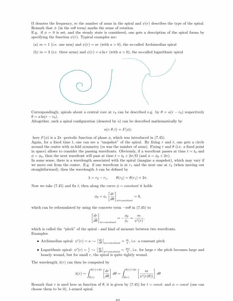
Ω denotes the frequency, m the number of arms in the spiral and ψ(r) describes the type of the spiral.Remark that ± (in the mθ term) marks the sense of rotation.E.g. if φ = 0 is set, and the steady state is considered, one gets a description of the spiral forms byspecifying the function ψ(r). Typical examples are:
(a) m = 1 (i.e. one arm) and ψ(r) = ar (with a > 0), the so-called Archimedian spiral
(b) m = 3 (i.e. three arms) and ψ(r) = a ln r (with a > 0), the so-called logarithmic spiral
Correspondingly, spirals about a central core at r0 can be described e.g. by θ = a(r − r0) respectivelyθ = a ln(r − r0).Altogether, such a spiral configuration (denoted by u) can be described mathematically by
u(r, θ, t) = F (φ);
here F (φ) is a 2π -periodic function of phase φ, which was introduced in (7.45).Again, for a fixed time t, one can see a “snapshot” of the spiral. By fixing r and t, one gets a circlearound the centre with m-fold symmetry (m was the number of arms). Fixing r and θ (i.e. a fixed pointin space) allows to consider the passing wavefronts. Obviously, if a wavefront passes at time t = t0 andφ = φ0, then the next wavefront will pass at time t = t0 + 2π/Ω (and φ = φ0 + 2π).In some sense, there is a wavelength associated with the spiral (imagine a snapshot), which may vary ifwe move out from the centre. E.g. if one wavefront is at r1 and the next one at r2 (when moving outstraightforward), then the wavelength λ can be defined by
λ = r2 − r1, θ(r2) = θ(r1) + 2π.
Now we take (7.45) and fix t, then along the curve φ = constant it holds
φθ + φr
[dr
dθ
]
φ=constant
= 0,
which can be reformulated by using the concrete term −mθ in (7.45) to
[dr
dθ
]
φ=constant
= −φθ
φr=
m
ψ′(r),
which is called the “pitch” of the spiral - and kind of measure between two wavefronts.Examples:
• Archimedian spiral: ψ′(r) = a ;
[drdθ
]
φ=constant= m
a , i.e. a constant pitch
• Logarithmic spiral: ψ′(r) = 1r ;
[drdθ
]
φ=constant= mr
a , i.e. for large r the pitch becomes large and
loosely wound, but for small r, the spiral is quite tightly wound.
The wavelength λ(r) can then be computed by
λ(r) =
∫ θ(r)+2π
θ(r)
[dr
dθ
]
dθ =
∫ θ(r)+2π
θ(r)
[m
ψ′(r(θ))
]
dθ
Remark that r is used here as function of θ, it is given by (7.45) for t = const. and φ = const (one canchoose them to be 0), 1-armed spiral.
83
As it is quite complicated to look for spiral wave solutions in general reaction diffusion systems andto analyse them, we consider here exemplarily the λ − ω system (which we know already a little bit, see(7.37)). It exhibits the main features and is still accessible by some analysis.
∂
∂t
(uv
)
=
(λ(a) −ω(a)ω(a) λ(a)
)(uv
)
+ D∆
(uv
)
, (7.46)
using here a2 = u2 + v2. u and v describe the reactant concentrations, ω(a) and λ(a) are real functionsof a, and ∆ denotes here the 2D Laplacian operator, i.e.
∆ =∂2
∂x2+
∂2
∂y2.
One important requirement is that in case of D = 0 (no diffusion) the remaining ODE system has a stablelimit cycle. For that, λ(a) needs an isolated zero (at a = a0 > 0) with dλ
da < 0 at a = 0 and ω(a0) 6= a0.Then, the limit cycle is u2 + v2 = a0 with the cycle frequency ω(a0).In the next step, we introduce the complex variable w = u + iv. The advantage is that we can write theλ-ω system (7.46) in a single complex equation:
∂w
∂t= (λ + iω)w + D∆w. (7.47)
For this system, we look for a solution of the form
w = A exp(iφ).
In this notation, A denotes the amplitude and φ the phase of the solution. As usual, this approach isinserted into (7.47) and we get:
∂A
∂texp(iφ) + iA exp(iφ)
∂φ
∂t= (λ + iω)A exp(iφ) + D∇ · (∇A · exp(iφ) + iA exp(iφ) · ∇φ)
= (λ + iω)A exp(iφ) + D∆A · exp(iφ) + D∇A · i exp(iφ)∇φ
+iD∇A · exp(iφ)∇φ + DAi2∇φ · ∇φ · exp(iφ) + DAi∆φ exp(iφ)
The term exp(iφ) can be cancelled out and we separate real and imaginary part:
∂A
∂t= λ(a)A + D∆A − DA|∇φ|2
A∂φ
∂t= ω(a)A + 2D(∇A · ∇φ) + DA∆φ
⇔ ∂φ
∂t= ω(a) + 2
D
A(∇A · ∇φ) + D∆φ.
Again we use polar coordinates as an appropriate coordinate system for spiral waves, i.e. we look forsolutions of the form
A = A(r), φ = Ωt + mθ + ψ(r).
Auxiliary reformulations (for the polar coordinates):
∆A =∂2A
∂r2+
1
r
∂A
∂r+
1
r2
∂2A
∂θ2︸ ︷︷ ︸
= 0 in our example
∆φ =∂2φ
∂r2+
1
r
∂φ
∂r+
1
r2
∂2φ
∂θ2=
d2ψ
dr2+
1
r
dψ
dr(in the example)
∇ =
(∂∂r
1r
∂∂θ
)
∇A =
(∂A∂r0
)
∇φ =
(∂φ∂r = dψ
dr1r m
)
.
84
(remark that ∂A∂t = 0 and ∂φ
∂t = Ω) .Using this approach and the polar coordinates we get as the two equations
0 = λ(a)A + D
(∂2A
∂r2+
1
r
∂A
∂r
)
− DA
(
(dψ
dr)2 +
m2
r2
)
Ω = ω(a) + 2D
A
(∂A
∂r· dψ
dr
)
+ D
(d2ψ
dr2+
1
r
dψ
dr
)
which can be rearranged to
Dd2A
dr2+
D
r
dA
dr+
(
λ(a) − D(dψ
dr)2 − Dm2
r2
)
A = 0 (7.48)
Dd2ψ
dr2+ D
(1
r+
”
A
dA
dr
)dψ
dr= Ω − ω(a) (7.49)
Equation (7.49) can be multiplied by rA2,
DrA2 d2ψ
dr2+ D(A2 + 2rA
dA
dr)dψ
dr︸ ︷︷ ︸
ddr
(DrA2 dψdr
)
= rA2(Ω − ω(a))
and integrated, this yields (have in mind that a corresponds to A)
dψ
dr=
1
DrA2(r)
∫ r
0
sA2(s)(Ω − ω(A(s))) ds
Next, we need BCs. Two main properties are required: The solutions have to be regular at r = 0 andbounded for r → ∞. For the regularity in (7.48) we have to get rid of the term −Dm2/r2 and with thisresult, the term with 2/A have to be brought to 0, thus
A(0) = 0,dψ
dr(0) = 0.
Assume that A → A∞ for r → ∞. From (7.49) we can use the asymptotic approximation
dψ
dr∼ 1
DrA2∞
∫ r
0
sA2∞(Ω − ω(A∞)) ds =
(Ω − ω(A∞))r
2D.
Obviously, dψdr is bounded if and only if Ω = ω(A∞); i.e. the amplitude of the spiral at infinity determines
the frequency).Letting r → ∞ in (7.48) it is
λ(A∞) − D
(dψ(∞)
dr
)2
= 0 ⇔ dψ(∞)
dr=
(λ(A∞)
D
)1/2
.
For considering the structure of the spiral near r = 0 we use a series of the following form:
A(r) = rc∞∑
n=0
anrn, a0 6= 0.
Auxiliary computations:
dA(r)
dr= crc−1
∞∑
n=0
anrn + rc∞∑
n=1
annrn−1
︸ ︷︷ ︸P
∞
n=0an+1(n+1)rn
d2A(r)
dr2= c(c − 1)rc−2
∞∑
n=0
anrn + 2crc−1∞∑
n=1
annrn−1
︸ ︷︷ ︸P
∞
n=0an+1(n+1)rn
+rc∞∑
n=1
an+1(n + 1)nrn−1
︸ ︷︷ ︸P
∞
n=0an+2(n+2)(n+1)rn
85
This is inserted into (7.48), compare the terms of the same power in r on both sides; for the lowest order(which is here rc−2) we find
D(c(c − 1)a0) + dCa0 − Dm2a0 = 0 ⇔ c(c − 1) + c − m2 = 0 ⇔ c2 − m2 = 0,
this condition has to be satisfied. We still want A to be regular at r = 0, thus we need c = m. Hence wefind (using w = A exp(iφ) and the spiral approach) for the structure of u and v near r = 0:
(uv
)
=
(rm cos(Ωt + mθ + ψ(0))rm sin(Ωt + mθ + ψ(0))
)
Remark that this is only a quite rough approximation. The correct analytic solutions of such systemsare quite difficult or even impossible to obtain; but of course it is possible to examine the structure bynumerical approaches. (Sometimes, one also uses such an approximate analysis for r → ∞).
Examples (taken from [12])):One example for a λ − ω system is
λ(a) = 1 − A2, ω(a) = −βA2
(a and A correspond to each other) with β > 0. E.g. 1-armed and 2-armed spirals can be computed ;
see Fig. 1.22 in [12]Another example for a λ − ω system:
λ(a) = ε − αA2, ω(a) = c − bA2,
with ε > 0 and α > 0. Using this example the w-equation (7.47) looks as follows (remark that A2 = |w|2):
wt = (λ + iω)w + D∆w
= (ε − αA2 + i(c − bA2))w + D∆w
= (ε + ic)w − (α + ib)|w|2w + D∆w.
Set w = weict (in some sense, this corresponds to setting c = 0), then we get (by wt = wteict + wiceict):
wteict + wiceict = (ε + ic)weict + (α + ib)|w|2weict + D∆weict
⇔ wt = εw + (α + ib)|w|2w + D∆w.
Next, we rescale w, t, and r according to
w =(α
ε
)1/2
w, t = εt, r =( ε
D
)1/2
r
and getwt = w − (1 + iβ)|w|2w + ∆w
(with β = b/α).Indeed, this system (the space-independent version of it, without ∆w) has a limit cycle solution whichreads
w = exp(−iβt).
Interestingly, for larger |β| the spiral waves become unstable (in a numerical investigation) and showsome chaotic behaviour, see e.g. Fig. 1.23 in [12].
86
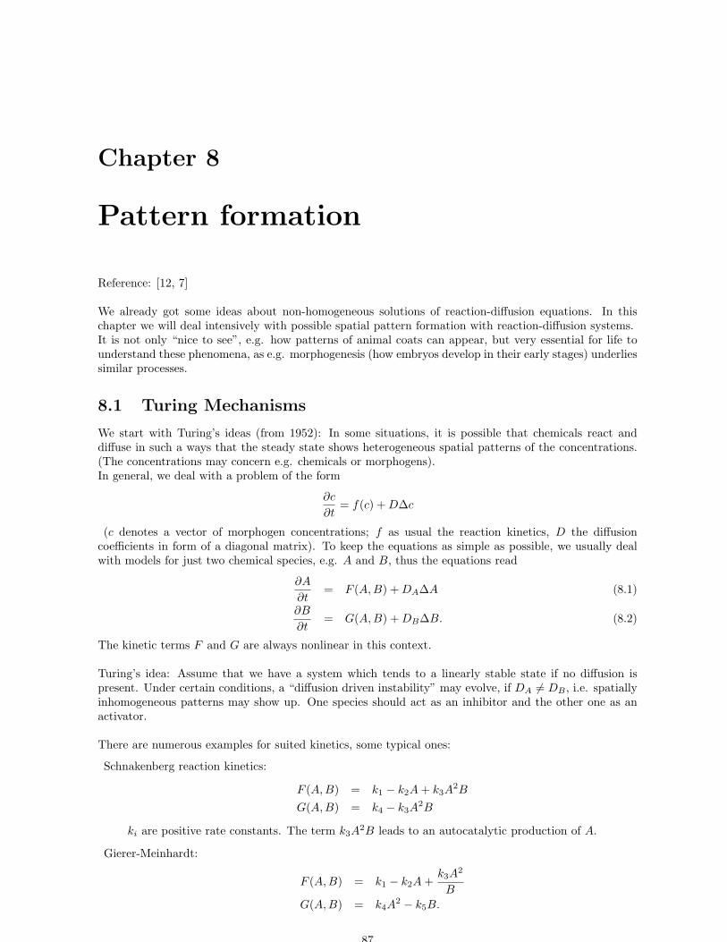
Chapter 8
Pattern formation
Reference: [12, 7]
We already got some ideas about non-homogeneous solutions of reaction-diffusion equations. In thischapter we will deal intensively with possible spatial pattern formation with reaction-diffusion systems.It is not only “nice to see”, e.g. how patterns of animal coats can appear, but very essential for life tounderstand these phenomena, as e.g. morphogenesis (how embryos develop in their early stages) underliessimilar processes.
8.1 Turing Mechanisms
We start with Turing’s ideas (from 1952): In some situations, it is possible that chemicals react anddiffuse in such a ways that the steady state shows heterogeneous spatial patterns of the concentrations.(The concentrations may concern e.g. chemicals or morphogens).In general, we deal with a problem of the form
∂c
∂t= f(c) + D∆c
(c denotes a vector of morphogen concentrations; f as usual the reaction kinetics, D the diffusioncoefficients in form of a diagonal matrix). To keep the equations as simple as possible, we usually dealwith models for just two chemical species, e.g. A and B, thus the equations read
∂A
∂t= F (A,B) + DA∆A (8.1)
∂B
∂t= G(A,B) + DB∆B. (8.2)
The kinetic terms F and G are always nonlinear in this context.
Turing’s idea: Assume that we have a system which tends to a linearly stable state if no diffusion ispresent. Under certain conditions, a “diffusion driven instability” may evolve, if DA 6= DB , i.e. spatiallyinhomogeneous patterns may show up. One species should act as an inhibitor and the other one as anactivator.
There are numerous examples for suited kinetics, some typical ones:
Schnakenberg reaction kinetics:
F (A,B) = k1 − k2A + k3A2B
G(A,B) = k4 − k3A2B
ki are positive rate constants. The term k3A2B leads to an autocatalytic production of A.
Gierer-Meinhardt:
F (A,B) = k1 − k2A +k3A
2
B
G(A,B) = k4A2 − k5B.
87
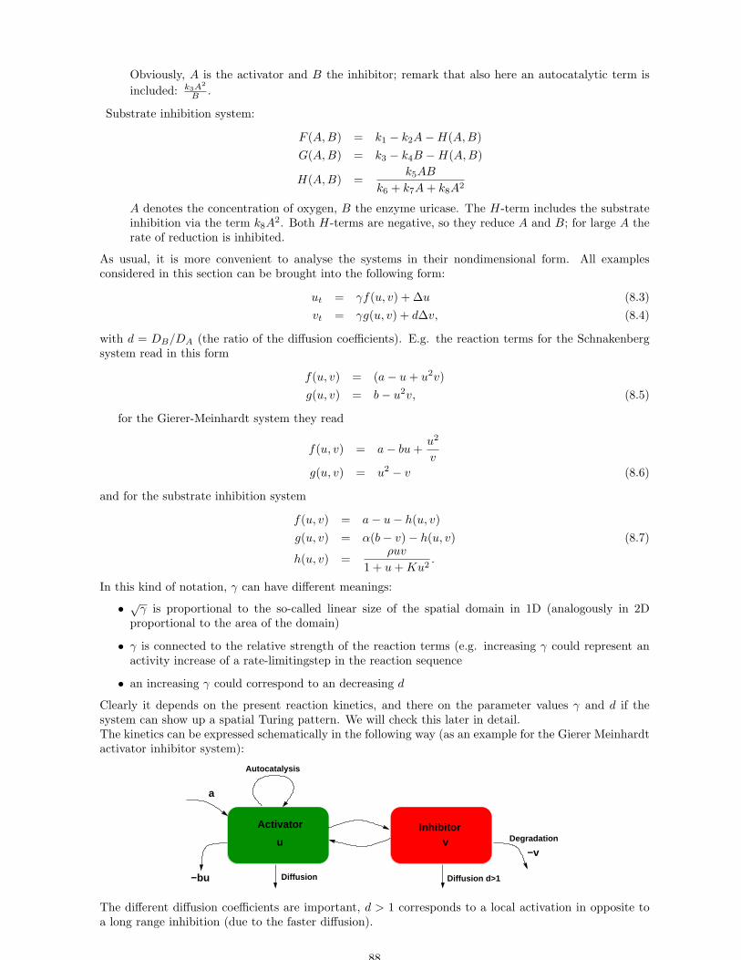
Obviously, A is the activator and B the inhibitor; remark that also here an autocatalytic term is
included: k3A2
B .
Substrate inhibition system:
F (A,B) = k1 − k2A − H(A,B)
G(A,B) = k3 − k4B − H(A,B)
H(A,B) =k5AB
k6 + k7A + k8A2
A denotes the concentration of oxygen, B the enzyme uricase. The H-term includes the substrateinhibition via the term k8A
2. Both H-terms are negative, so they reduce A and B; for large A therate of reduction is inhibited.
As usual, it is more convenient to analyse the systems in their nondimensional form. All examplesconsidered in this section can be brought into the following form:
ut = γf(u, v) + ∆u (8.3)
vt = γg(u, v) + d∆v, (8.4)
with d = DB/DA (the ratio of the diffusion coefficients). E.g. the reaction terms for the Schnakenbergsystem read in this form
f(u, v) = (a − u + u2v)
g(u, v) = b − u2v, (8.5)
for the Gierer-Meinhardt system they read
f(u, v) = a − bu +u2
v
g(u, v) = u2 − v (8.6)
and for the substrate inhibition system
f(u, v) = a − u − h(u, v)
g(u, v) = α(b − v) − h(u, v) (8.7)
h(u, v) =ρuv
1 + u + Ku2.
In this kind of notation, γ can have different meanings:
• √γ is proportional to the so-called linear size of the spatial domain in 1D (analogously in 2D
proportional to the area of the domain)
• γ is connected to the relative strength of the reaction terms (e.g. increasing γ could represent anactivity increase of a rate-limitingstep in the reaction sequence
• an increasing γ could correspond to an decreasing d
Clearly it depends on the present reaction kinetics, and there on the parameter values γ and d if thesystem can show up a spatial Turing pattern. We will check this later in detail.The kinetics can be expressed schematically in the following way (as an example for the Gierer Meinhardtactivator inhibitor system):
Diffusion Diffusion d>1
a
−bu
Degradation
−v
Autocatalysis
u v
Activator Inhibitor
The different diffusion coefficients are important, d > 1 corresponds to a local activation in opposite toa long range inhibition (due to the faster diffusion).
88
8.2 Linear stability analysis for Diffusion-driven instability
The aim of this section is to find necessary and sufficient conditions for the above-mentioned diffusion-driven instability of the homogeneous steady state and how a spatial pattern can be initiated. As usualwe need initial conditions (just assumed to be u(r, 0), v(r, 0)) and boundary conditions: We choose zeroflux boundary conditions, so patterns are not caused by external input, but by ”self-organisation”, i.e.
(n · ∇)
(uv
)
= 0
n denotes the outer normal to ∂B, the closed boundary of the considered domain B.The considered homogeneous steady state (u0, v0) corresponds to the positive solution of
f(u, v) = 0, g(u, v) = 0.
Goal is to find a linear instability of this steady state which is only spatially dependent. That means,as already mentioned that the homogeneous steady state must be linearly stable if diffusion (i.e. spatialvariation) is absent. The procedure for this is already well-known, the reaction equations (i.e. thespatially homogeneous problem) read
ut = γf(u, v), vt = γg(u, v).
We use the linearisation at (u0, v0): w =
(u − u0
v − v0
)
, which yields the linear system
wt = γAw, with A =
(fu fv
gu gv
)
u0,v0
and we look for solutions w which are proportional to eλt, λ eigenvalue of A. The eigenvalues here canbe computed in the standard way
λ2 − γ(fu + gv)λ + γ2(fugv)λ + γ2(fugv − fvgu) = 0 (8.8)
and readλ1, λ2 =
γ
2
(
(fu + gv) ±√
(fu + gv)2 − 4(fugv − fvgu))
.
Reλ < 0 guarantees stability, i.e.
trA = fu + gv < 0 and detA = fugv − fvgu > 0.
Of course, the coordinates of the steady state, (u0, v0) depend on the kinetic parameters, so the inequal-ities for the trace and the determinant imply constraints on the parameters. (Even the plots of isoclinesin the phase space can help here!)
In the next step, we use the whole system, including diffusion. Linearisation at the steady state (u0, v0)or in the w-coordinates w = 0 looks as follows:
wt = γAw + D∆w, with D =
(1 00 d
)
. (8.9)
As a first step, we consider the time-independent solution W (r) of the spatial eigenvalue problem
∆W + k2W = 0
(n · ∇)W = 0 for r on ∂B (boundary conditions)
k is the eigenvalue. For the 1D case (e.g. 0 ≤ x ≤ α) the eigenfunctions W = cos(nπx/a) (n integer)satisfy the zero flux conditions at x = 0 and x = a; the corresponding eigenvalues are k = nπ/a. Inthis context, k is called the wavenumber, vice versa 1
k = anπ is a measure of the wavelike pattern (and
proportional to the wavelength ω = 2πk = 2a
n . As long as we deal with finite domains, there is a discreteset of possible wavenumbers.So, let Wk(r) denote the eigenfunction which belongs to wavenumber k (it satisfies the zero flux boundarycondition!). We deal with a linear problem, so the solutions w(r, t) of (8.9) can be displayed as
w(r, t) =∑
k
ckeλtWk(r),
89
here, the constants ck can be determined by a Fourier expansion of the initial condition in terms of thetime-independent solutions Wk(r). Remark that λ denotes the eigenvalue for the temporal growth (notto mix it up with the “spatial eigenvalue problem”)!We take this approach and insert it into (8.9) and take into account the properties of Wk and get foreach k:
λWk = γAWk + D∆Wk
= γAWk − Dk2Wk.
(The term eλt appears in each term and can thus be cancelled out). Wk are required to be nontrivialsolutions, thus we determine λ as roots of the characteristic polynomial
det(λI − γA + Dk2) = 0.
Using the definitions of the matrices A and D from above, this corresponds to
λ2 + λ[k2(1 + d) − γ(fu + gv)] + h(k2) = 0, (8.10)
whereh(k2) = dk4 − γ(dfu + gv)k2 + γ2detA.
As usual, the steady state (u0, v0) is (linearly) stable if Reλ < 0 for both eigenvalues λ.Remark that we wanted to have a stable steady state in case of absent spatial effects, which correspondsto Reλ(k2 = 0) < 0, which again corresponds to (8.8) and leads to the conditions for the trace andthe determinant above. Second, we require Reλ(k) > 0 for a k 6= 0, i.e. such that the steady stateis unstable if spatial disturbances (i.e. the diffusion) are present. There are two possibilities for this:Either k2(1+d)−γ(fu + gv) is negative (which corresponds to the coefficient of λ in (8.10)) or h(k2) < 0for some k 6= 0. From the trace condition (for the case without diffusion) we have (fu + gv) < 0, andk2(1 + d) > 0 for all k 6= 0 (generally true), thus we find
(k2(1 + d) − γ(fu + gv)) > 0,
thus the coefficient for λ is always positive. The only remaining possibility for Reλ(k2) is hence h(k2) < 0for some k.It is useful to consider the explicit formula for λ (solution of (8.10)):
2λ = −(k2(1 + d) − γ(fu + gv)) ±√
(k2(1 + d) − γ(fu + gv))2 − 4h(k2).
h was defined as h(k2) = dk4 − γ(dfu + gv)k2 + γ2detA. The determinant of A was needed to be positive(for the stability of the non-spatial problem), so we need (dfu + gv) > 0. From the trace condition(fu + gv < 0) it implies that d 6= 1 and fu and gv need opposite signs to allow for this condition.Short excurs to the kinetics of the Schnakenberg system: the stationary state for the kinetics can beeasily computed via
f(u0, v0) = a − u0 + u20v0 = 0 and g(u0, v0) = b − u2
0v0 = 0
to be
u0 = b + a, v0 =b
(a + b)2
where b > 0 and a + b > 0. Hence, we find at the stationary point:
fu|(u0,v0) = −1 + 2u0v0 = −1 + 2(b + a) · b
(a + b)2=
b − a
a + b
gv = −u20 = −(b + a)2 < 0
For the linear stability of the non-diffusive model, we claimed that fu + gv < 0, so in this case we havefu > 0. In order to allow for dfu + gv > 0, then we need d > 1. What does this mean? The diffusion ofthe inhibitor must be faster than the diffusion of the activator!
Still we have not found a sufficient condition for Reλ > 0 (only a necessary condition). In order toget a negative h(k2) for some k, the minimum hmin must be negative. Setting the first derivative of h to0,
h′ = 2dk2 − γ(dfu + gv) = 0 ⇔ k2 = k2m =
γ(dfu + gv)
2d
90
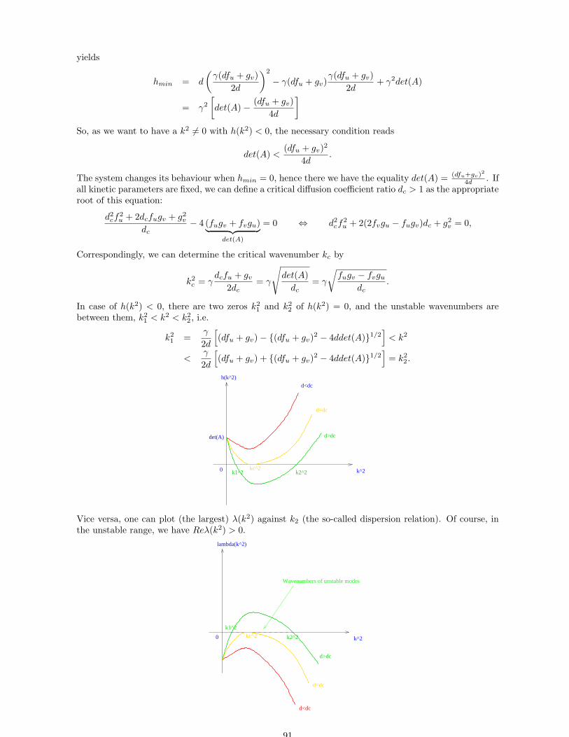
yields
hmin = d
(γ(dfu + gv)
2d
)2
− γ(dfu + gv)γ(dfu + gv)
2d+ γ2det(A)
= γ2
[
det(A) − (dfu + gv)
4d
]
So, as we want to have a k2 6= 0 with h(k2) < 0, the necessary condition reads
det(A) <(dfu + gv)2
4d.
The system changes its behaviour when hmin = 0, hence there we have the equality det(A) = (dfu+gv)2
4d . Ifall kinetic parameters are fixed, we can define a critical diffusion coefficient ratio dc > 1 as the appropriateroot of this equation:
d2cf
2u + 2dcfugv + g2
v
dc− 4 (fugv + fvgu)
︸ ︷︷ ︸
det(A)
= 0 ⇔ d2cf
2u + 2(2fvgu − fugv)dc + g2
v = 0,
Correspondingly, we can determine the critical wavenumber kc by
k2c = γ
dcfu + gv
2dc= γ
√
det(A)
dc= γ
√
fugv − fvgu
dc.
In case of h(k2) < 0, there are two zeros k21 and k2
2 of h(k2) = 0, and the unstable wavenumbers arebetween them, k2
1 < k2 < k22, i.e.
k21 =
γ
2d
[
(dfu + gv) − (dfu + gv)2 − 4ddet(A)1/2]
< k2
<γ
2d
[
(dfu + gv) + (dfu + gv)2 − 4ddet(A)1/2]
= k22.
d=dc
d>dc
d<dc
det(A)
0 k^2k1^2 k2^2
h(k^2)
kc^2
Vice versa, one can plot (the largest) λ(k2) against k2 (the so-called dispersion relation). Of course, inthe unstable range, we have Reλ(k2) > 0.
0 k^2kc^2
d>dc
k2^2
d=dc
d<dc
k1^2
lambda(k^2)
Wavenumbers of unstable modes
91
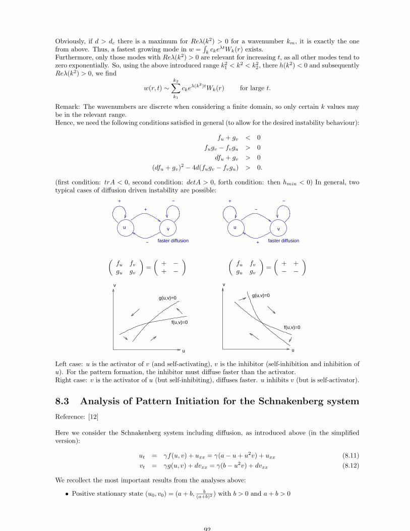
Obviously, if d > dc there is a maximum for Reλ(k2) > 0 for a wavenumber km, it is exactly the onefrom above. Thus, a fastest growing mode in w =
∫
kckeλtWk(r) exists.
Furthermore, only those modes with Reλ(k2) > 0 are relevant for increasing t, as all other modes tend tozero exponentially. So, using the above introduced range k2
1 < k2 < k22, there h(k2) < 0 and subsequently
Reλ(k2) > 0, we find
w(r, t) ∼k2∑
k1
ckeλ(k2)tWk(r) for large t.
Remark: The wavenumbers are discrete when considering a finite domain, so only certain k values maybe in the relevant range.Hence, we need the following conditions satisfied in general (to allow for the desired instability behaviour):
fu + gv < 0
fugv − fvgu > 0
dfu + gv > 0
(dfu + gv)2 − 4d(fugv − fvgu) > 0.
(first condition: trA < 0, second condition: detA > 0, forth condition: then hmin < 0) In general, twotypical cases of diffusion driven instability are possible:
u v
−
+
+ −
faster diffusion
u v
+ −
faster diffusion
−
+
(fu fv
gu gv
)
=
(+ −+ −
) (fu fv
gu gv
)
=
(+ +− −
)
u
v
f(u,v)=0
g(u,v)=0
u
v
f(u,v)=0
g(u,v)=0
Left case: u is the activator of v (and self-activating), v is the inhibitor (self-inhibition and inhibition ofu). For the pattern formation, the inhibitor must diffuse faster than the activator.Right case: v is the activator of u (but self-inhibiting), diffuses faster. u inhibits v (but is self-activator).
8.3 Analysis of Pattern Initiation for the Schnakenberg system
Reference: [12]
Here we consider the Schnakenberg system including diffusion, as introduced above (in the simplifiedversion):
ut = γf(u, v) + uxx = γ(a − u + u2v) + uxx (8.11)
vt = γg(u, v) + dvxx = γ(b − u2v) + dvxx (8.12)
We recollect the most important results from the analyses above:
• Positive stationary state (u0, v0) = (a + b, b(a+b)2 ) with b > 0 and a + b > 0
92
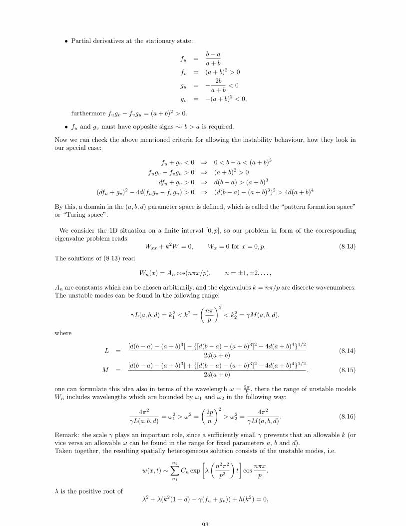
• Partial derivatives at the stationary state:
fu =b − a
a + b
fv = (a + b)2 > 0
gu = − 2b
a + b< 0
gv = −(a + b)2 < 0,
furthermore fugv − fvgu = (a + b)2 > 0.
• fu and gv must have opposite signs ; b > a is required.
Now we can check the above mentioned criteria for allowing the instability behaviour, how they look inour special case:
fu + gv < 0 ⇒ 0 < b − a < (a + b)3
fugv − fvgu > 0 ⇒ (a + b)2 > 0
dfu + gv > 0 ⇒ d(b − a) > (a + b)3
(dfu + gv)2 − 4d(fugv − fvgu) > 0 ⇒ (d(b − a) − (a + b)3)2 > 4d(a + b)4
By this, a domain in the (a, b, d) parameter space is defined, which is called the “pattern formation space”or “Turing space”.
We consider the 1D situation on a finite interval [0, p], so our problem in form of the correspondingeigenvalue problem reads
Wxx + k2W = 0, Wx = 0 for x = 0, p. (8.13)
The solutions of (8.13) read
Wn(x) = An cos(nπx/p), n = ±1,±2, . . . ,
An are constants which can be chosen arbitrarily, and the eigenvalues k = nπ/p are discrete wavenumbers.The unstable modes can be found in the following range:
γL(a, b, d) = k21 < k2 =
(nπ
p
)2
< k22 = γM(a, b, d),
where
L =[d(b − a) − (a + b)3] − [d(b − a) − (a + b)3]2 − 4d(a + b)41/2
2d(a + b)(8.14)
M =[d(b − a) − (a + b)3] + [d(b − a) − (a + b)3]2 − 4d(a + b)41/2
2d(a + b). (8.15)
one can formulate this idea also in terms of the wavelength ω = 2πk , there the range of unstable models
Wn includes wavelengths which are bounded by ω1 and ω2 in the following way:
4π2
γL(a, b, d)= ω2
1 > ω2 =
(2p
n
)2
> ω22 =
4π2
γM(a, b, d). (8.16)
Remark: the scale γ plays an important role, since a sufficiently small γ prevents that an allowable k (orvice versa an allowable ω can be found in the range for fixed parameters a, b and d).Taken together, the resulting spatially heterogeneous solution consists of the unstable modes, i.e.
w(x, t) ∼n2∑
n1
Cn exp
[
λ
(n2π2
p2
)
t
]
cosnπx
p.
λ is the positive root ofλ2 + λ(k2(1 + d) − γ(fu + gv)) + h(k2) = 0,
93
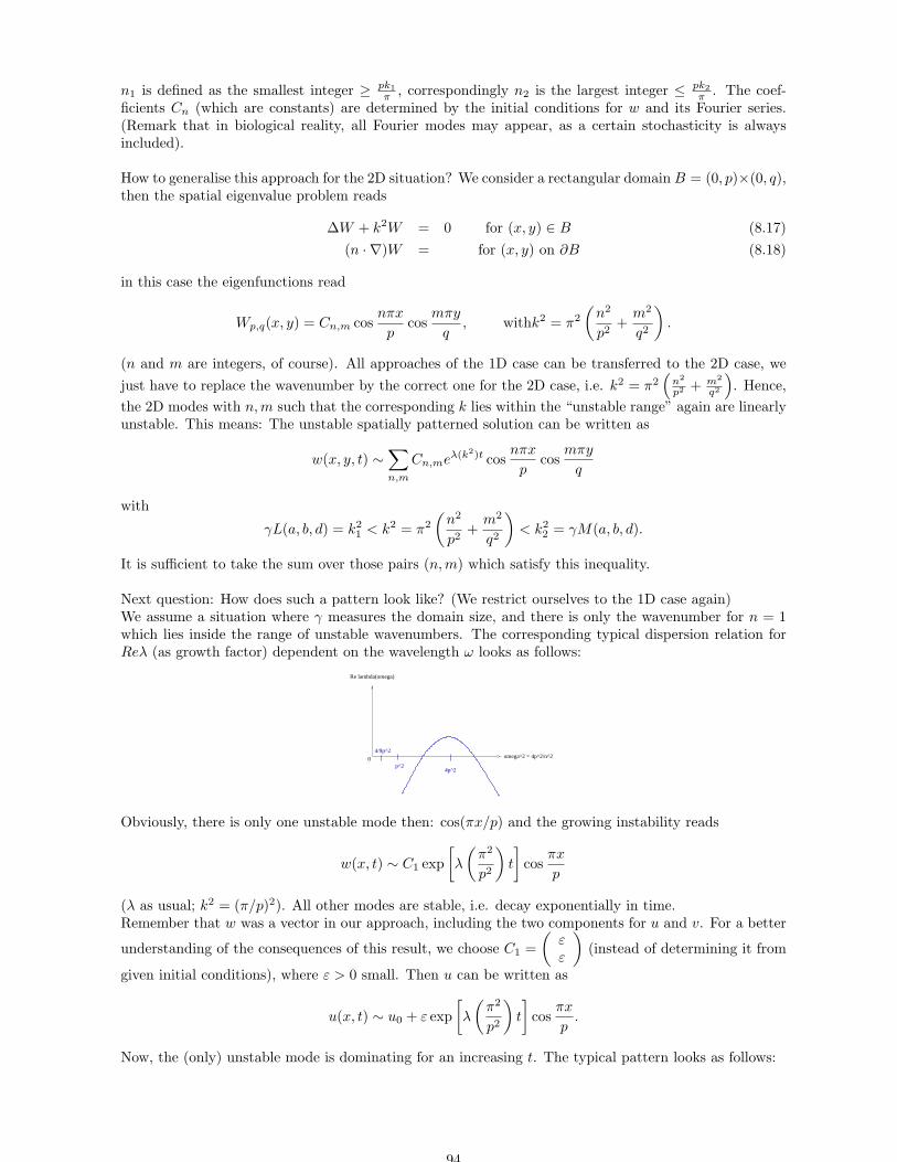
n1 is defined as the smallest integer ≥ pk1
π , correspondingly n2 is the largest integer ≤ pk2
π . The coef-ficients Cn (which are constants) are determined by the initial conditions for w and its Fourier series.(Remark that in biological reality, all Fourier modes may appear, as a certain stochasticity is alwaysincluded).
How to generalise this approach for the 2D situation? We consider a rectangular domain B = (0, p)×(0, q),then the spatial eigenvalue problem reads
∆W + k2W = 0 for (x, y) ∈ B (8.17)
(n · ∇)W = for (x, y) on ∂B (8.18)
in this case the eigenfunctions read
Wp,q(x, y) = Cn,m cosnπx
pcos
mπy
q, withk2 = π2
(n2
p2+
m2
q2
)
.
(n and m are integers, of course). All approaches of the 1D case can be transferred to the 2D case, we
just have to replace the wavenumber by the correct one for the 2D case, i.e. k2 = π2(
n2
p2 + m2
q2
)
. Hence,
the 2D modes with n,m such that the corresponding k lies within the “unstable range” again are linearlyunstable. This means: The unstable spatially patterned solution can be written as
w(x, y, t) ∼∑
n,m
Cn,meλ(k2)t cosnπx
pcos
mπy
q
with
γL(a, b, d) = k21 < k2 = π2
(n2
p2+
m2
q2
)
< k22 = γM(a, b, d).
It is sufficient to take the sum over those pairs (n,m) which satisfy this inequality.
Next question: How does such a pattern look like? (We restrict ourselves to the 1D case again)We assume a situation where γ measures the domain size, and there is only the wavenumber for n = 1which lies inside the range of unstable wavenumbers. The corresponding typical dispersion relation forReλ (as growth factor) dependent on the wavelength ω looks as follows:
0 omega^2 = 4p^2/n^2
4p^2p^2
4/9p^2
Re lambda(omega)
Obviously, there is only one unstable mode then: cos(πx/p) and the growing instability reads
w(x, t) ∼ C1 exp
[
λ
(π2
p2
)
t
]
cosπx
p
(λ as usual; k2 = (π/p)2). All other modes are stable, i.e. decay exponentially in time.Remember that w was a vector in our approach, including the two components for u and v. For a better
understanding of the consequences of this result, we choose C1 =
(εε
)
(instead of determining it from
given initial conditions), where ε > 0 small. Then u can be written as
u(x, t) ∼ u0 + ε exp
[
λ
(π2
p2
)
t
]
cosπx
p.
Now, the (only) unstable mode is dominating for an increasing t. The typical pattern looks as follows:
94
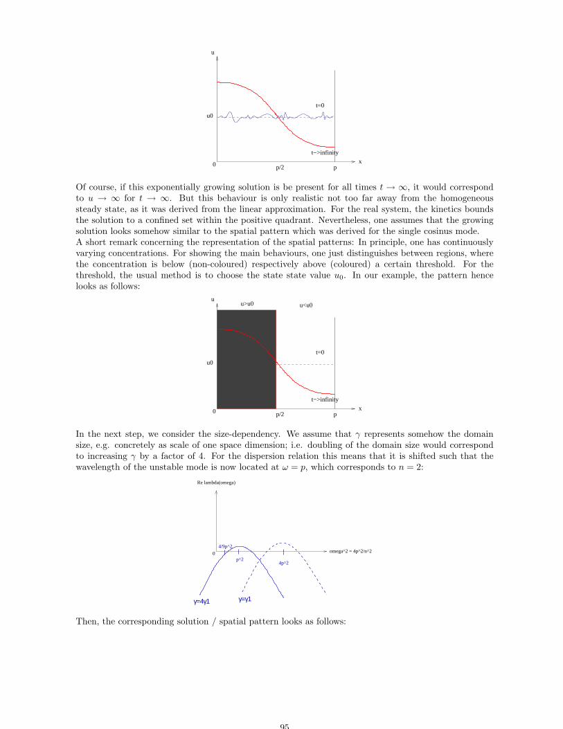
xpp/2
u0
t=0
t−>infinity
u
0
Of course, if this exponentially growing solution is be present for all times t → ∞, it would correspondto u → ∞ for t → ∞. But this behaviour is only realistic not too far away from the homogeneoussteady state, as it was derived from the linear approximation. For the real system, the kinetics boundsthe solution to a confined set within the positive quadrant. Nevertheless, one assumes that the growingsolution looks somehow similar to the spatial pattern which was derived for the single cosinus mode.A short remark concerning the representation of the spatial patterns: In principle, one has continuouslyvarying concentrations. For showing the main behaviours, one just distinguishes between regions, wherethe concentration is below (non-coloured) respectively above (coloured) a certain threshold. For thethreshold, the usual method is to choose the state state value u0. In our example, the pattern hencelooks as follows:
xpp/2
u0
t=0
t−>infinity
u
0
u>u0 u<u0
In the next step, we consider the size-dependency. We assume that γ represents somehow the domainsize, e.g. concretely as scale of one space dimension; i.e. doubling of the domain size would correspondto increasing γ by a factor of 4. For the dispersion relation this means that it is shifted such that thewavelength of the unstable mode is now located at ω = p, which corresponds to n = 2:
0 omega^2 = 4p^2/n^2
4p^2p^2
4/9p^2
Re lambda(omega)
γ=4γ1 γ=γ1
Then, the corresponding solution / spatial pattern looks as follows:
95
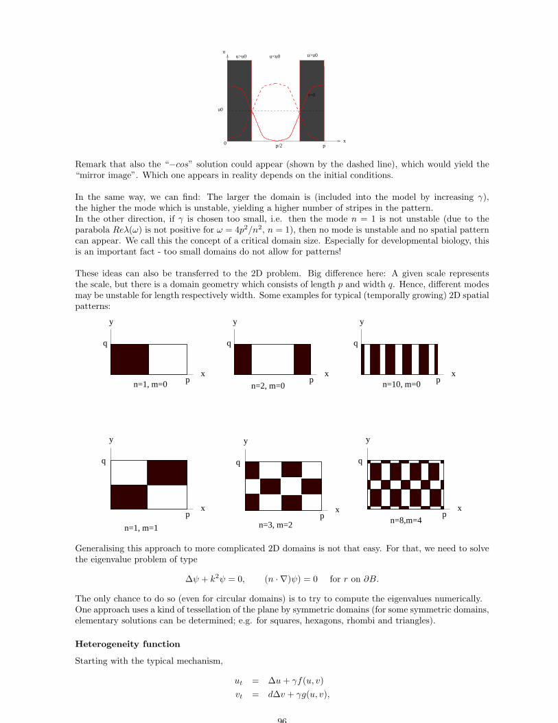
xpp/2
t=0
u
0
u0
u>u0 u<u0 u>u0
Remark that also the “−cos” solution could appear (shown by the dashed line), which would yield the“mirror image”. Which one appears in reality depends on the initial conditions.
In the same way, we can find: The larger the domain is (included into the model by increasing γ),the higher the mode which is unstable, yielding a higher number of stripes in the pattern.In the other direction, if γ is chosen too small, i.e. then the mode n = 1 is not unstable (due to theparabola Reλ(ω) is not positive for ω = 4p2/n2, n = 1), then no mode is unstable and no spatial patterncan appear. We call this the concept of a critical domain size. Especially for developmental biology, thisis an important fact - too small domains do not allow for patterns!
These ideas can also be transferred to the 2D problem. Big difference here: A given scale representsthe scale, but there is a domain geometry which consists of length p and width q. Hence, different modesmay be unstable for length respectively width. Some examples for typical (temporally growing) 2D spatialpatterns:
y
xp
q
y
xp
q
y
xp
q
xp
y
q
xp
y
q
xp
y
q
n=1, m=0 n=2, m=0 n=10, m=0
n=1, m=1 n=3, m=2 n=8,m=4
Generalising this approach to more complicated 2D domains is not that easy. For that, we need to solvethe eigenvalue problem of type
∆ψ + k2ψ = 0, (n · ∇)ψ) = 0 for r on ∂B.
The only chance to do so (even for circular domains) is to try to compute the eigenvalues numerically.One approach uses a kind of tessellation of the plane by symmetric domains (for some symmetric domains,elementary solutions can be determined; e.g. for squares, hexagons, rhombi and triangles).
Heterogeneity function
Starting with the typical mechanism,
ut = ∆u + γf(u, v)
vt = d∆v + γg(u, v),
96
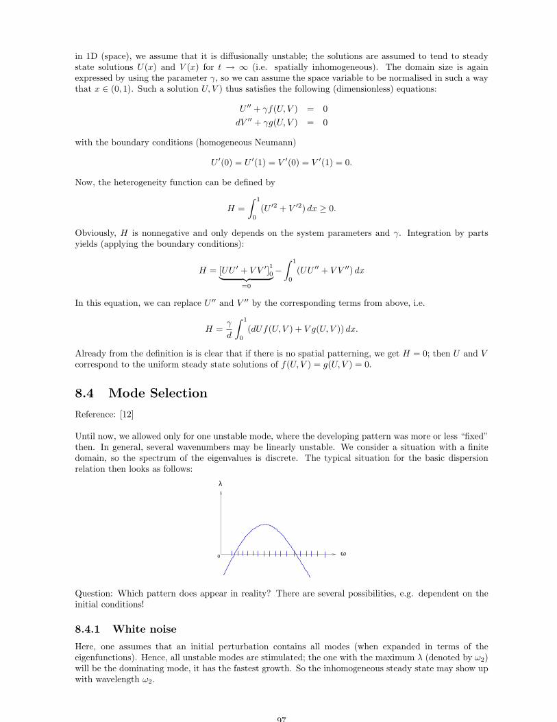
in 1D (space), we assume that it is diffusionally unstable; the solutions are assumed to tend to steadystate solutions U(x) and V (x) for t → ∞ (i.e. spatially inhomogeneous). The domain size is againexpressed by using the parameter γ, so we can assume the space variable to be normalised in such a waythat x ∈ (0, 1). Such a solution U, V ) thus satisfies the following (dimensionless) equations:
U ′′ + γf(U, V ) = 0
dV ′′ + γg(U, V ) = 0
with the boundary conditions (homogeneous Neumann)
U ′(0) = U ′(1) = V ′(0) = V ′(1) = 0.
Now, the heterogeneity function can be defined by
H =
∫ 1
0
(U ′2 + V ′2) dx ≥ 0.
Obviously, H is nonnegative and only depends on the system parameters and γ. Integration by partsyields (applying the boundary conditions):
H = [UU ′ + V V ′]10
︸ ︷︷ ︸
=0
−∫ 1
0
(UU ′′ + V V ′′) dx
In this equation, we can replace U ′′ and V ′′ by the corresponding terms from above, i.e.
H =γ
d
∫ 1
0
(dUf(U, V ) + V g(U, V )) dx.
Already from the definition is is clear that if there is no spatial patterning, we get H = 0; then U and Vcorrespond to the uniform steady state solutions of f(U, V ) = g(U, V ) = 0.
8.4 Mode Selection
Reference: [12]
Until now, we allowed only for one unstable mode, where the developing pattern was more or less “fixed”then. In general, several wavenumbers may be linearly unstable. We consider a situation with a finitedomain, so the spectrum of the eigenvalues is discrete. The typical situation for the basic dispersionrelation then looks as follows:
0 ω
λ
Question: Which pattern does appear in reality? There are several possibilities, e.g. dependent on theinitial conditions!
8.4.1 White noise
Here, one assumes that an initial perturbation contains all modes (when expanded in terms of theeigenfunctions). Hence, all unstable modes are stimulated; the one with the maximum λ (denoted by ω2)will be the dominating mode, it has the fastest growth. So the inhomogeneous steady state may show upwith wavelength ω2.
97
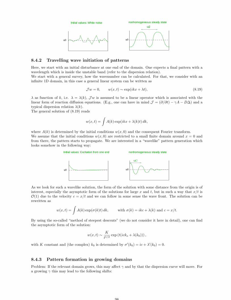
u0 u0
ω2Initial values: White noise nonhomogeneous steady state
8.4.2 Travelling wave initiation of patterns
Here, we start with an initial disturbance at one end of the domain. One expects a final pattern with awavelength which is inside the unstable band (refer to the dispersion relation).We start with a general survey, how the wavenumber can be calculated. For that, we consider with aninfinite 1D domain, in this case a general linear system can be written as
Jw = 0, w(x, t) ∼ exp(ikx + λt), (8.19)
λ as function of k, i.e. λ = λ(k), Jw is assumed to be a linear operator which is associated with thelinear form of reaction diffusion equations. (E.g., one can have in mind J = (∂/∂t) − γA − D∆) and atypical dispersion relation λ(k).The general solution of (8.19) reads
w(x, t) =
∫
A(k) exp(ikx + λ(k)t) dk,
where A(k) is determined by the initial conditions w(x, 0) and the consequent Fourier transform.We assume that the initial conditions w(x, 0) are restricted to a small finite domain around x = 0 andfrom there, the pattern starts to propagate. We are interested in a “wavelike” pattern generation whichlooks somehow in the following way:
u0 u0
nonhomogeneous steady state
ω∗
Initial values: Excitation from one end
As we look for such a wavelike solution, the form of the solution with some distance from the origin is ofinterest, especially the asymptotic form of the solutions for large x and t, but in such a way that x/t isO(1) due to the velocity c = x/t and we can follow in some sense the wave front. The solution can berewritten as
w(x, t) =
∫
A(k) exp(σ(k)t) dk, with σ(k) = ikc + λ(k) and c = x/t.
By using the so-called “method of steepest descents” (we do not consider it here in detail), one can findthe asymptotic form of the solution:
w(x, t) ∼ K
t1/2exp (t(icko + λ(k0))) ,
with K constant and (the complex) k0 is determined by σ′(k0) = ic + λ′(k0) = 0.
8.4.3 Pattern formation in growing domains
Problem: If the relevant domain grows, this may affect γ and by that the dispersion curve will move. Fora growing γ this may lead to the following shifts:
98
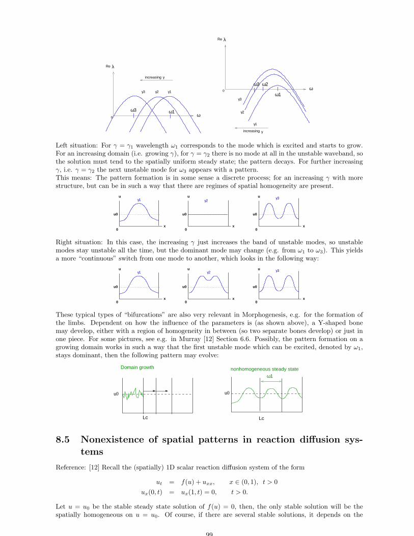
0 ω
λRe
ω1
increasing γ
γ1γ2γ3
ω3
0 ω
λRe
ω3 ω2
γincreasing
γ3
γ2
γ1
ω1
Left situation: For γ = γ1 wavelength ω1 corresponds to the mode which is excited and starts to grow.For an increasing domain (i.e. growing γ), for γ = γ2 there is no mode at all in the unstable waveband, sothe solution must tend to the spatially uniform steady state; the pattern decays. For further increasingγ, i.e. γ = γ2 the next unstable mode for ω3 appears with a pattern.This means: The pattern formation is in some sense a discrete process; for an increasing γ with morestructure, but can be in such a way that there are regimes of spatial homogeneity are present.
u
0x
u0
u
0x
u0
u
0x
u0
γ1 γ2γ3
Right situation: In this case, the increasing γ just increases the band of unstable modes, so unstablemodes stay unstable all the time, but the dominant mode may change (e.g. from ω1 to ω3). This yieldsa more “continuous” switch from one mode to another, which looks in the following way:
u
0x
u0
u
0x
u0
u
0x
u0
γ1 γ3γ2
These typical types of “bifurcations” are also very relevant in Morphogenesis, e.g. for the formation ofthe limbs. Dependent on how the influence of the parameters is (as shown above), a Y-shaped bonemay develop, either with a region of homogeneity in between (so two separate bones develop) or just inone piece. For some pictures, see e.g. in Murray [12] Section 6.6. Possibly, the pattern formation on agrowing domain works in such a way that the first unstable mode which can be excited, denoted by ω1,stays dominant, then the following pattern may evolve:
u0 u0
ω1
LcLc
Domain growth nonhomogeneous steady state
8.5 Nonexistence of spatial patterns in reaction diffusion sys-tems
Reference: [12] Recall the (spatially) 1D scalar reaction diffusion system of the form
ut = f(u) + uxx, x ∈ (0, 1), t > 0
ux(0, t) = ux(1, t) = 0, t > 0.
Let u = u0 be the stable steady state solution of f(u) = 0, then, the only stable solution will be thespatially homogeneous on u = u0. Of course, if there are several stable solutions, it depends on the
99

initial conditions, which one will be assumed. In the 1D case (spatial dimension) one can show that anyspatially nonhomogeneous steady state solution is unstable.In higher spatial dimensions this mustn’t be true, when f(u) has two linearly stable steady states. Apattern may evolve, it depends on the specific domain boundaries (e.g. nonconvex boundaries), howmuch “transport” is possible from one steady state to another an so on.
In this section, we consider shortly the case of large diffusion. Of course, for the pattern formationit was necessary to have different diffusion coefficients for different reactants in the reaction diffusionsystem. But what happens is the diffusion becomes very large? Will it destroy patterns?
We start with a two-species system:
ut = f(u, v) + D1uxx (8.20)
vt = g(u, v) + D2vxx (8.21)
and assume homogeneous Neumann boundary conditions and initial conditions as follows:
ux(0, t) = ux(1, t) = vx(0, t) = vx(1, t) = 0
u(x, 0) = u0(x)
v(x, 0) = v0(x).
For compatibility of the initial and the boundary conditions, we claim that u′0(x) = v′
0(x) = 0 on x = 0, 1.Next, a so-called energy integral E is defined as follows:
E(t) =1
2
∫ 1
0
(u2x + v2
x) dx.
(Remark that this corresponds exactly to the heterogeneity function, except for the factor 12 .)
The t-derivative readsdE
dt=
∫ 1
0
(uxuxt + vxvxt) dx
We can take (8.20) and (8.21), derive it with respect to x and insert it into this equation (use partialintegration and the zero flux boundary conditions):
dE
dt=
∫ 1
0
[ux(D1uxx)x + ux(fuux + fvvx) + vx(D2vxx)x + vx(guux + gvvx)] dx
= [uxD1uxx + vxD2vxx]10
︸ ︷︷ ︸
=0
−∫ 1
0
(D1u2xx + D2v
2xx) dx
+
∫ 1
0
[fuu2
X + gvv2x + (fv + gu)uxvx
]dx.
For simplification of the notation, we introduce
d = min(D1,D2), m = maxu,v
(f2
u + f2v + g2
u + g2v
)(1/2),
the maxu,v means that all possible solution values for u and v are taken and the maximum is deter-mined over these. Hence we can formulate the following estimate (remember the Poincare inequality:∫ 1
0u2
xx dx ≥ π2∫ 1
0u2
X dx):
dE
dt≤ −d
∫ 1
0
(u2xx + v2
xx) dx + 4m
∫ 1
0
(u2x + v2
X) dx
≤ (4m − 2π2d)E
This estimation has to be considered carefully: If d is so large that (4m − 2π2d) < 0, then we obviouslyget dE
dt < 0 and consequently E → 0 for t → ∞ (by definition it is E(t) ≥ 0). But, having in mind thedefinition of E, this implies that ux → 0 and vx → 0 which means spatial homogeneity in the solution.Remark that this is just an example, no “if and only if situation”, we have used estimations which canbe chosen differently.
100
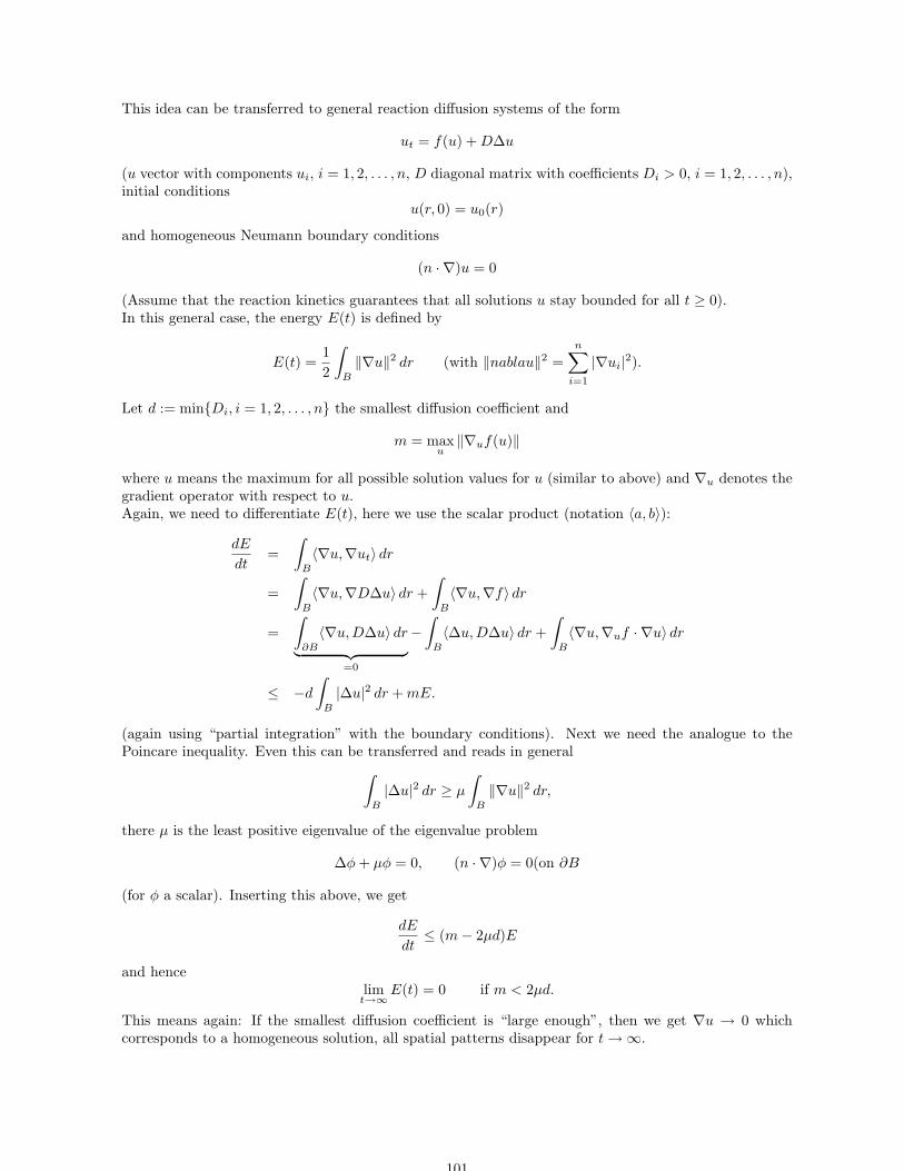
This idea can be transferred to general reaction diffusion systems of the form
ut = f(u) + D∆u
(u vector with components ui, i = 1, 2, . . . , n, D diagonal matrix with coefficients Di > 0, i = 1, 2, . . . , n),initial conditions
u(r, 0) = u0(r)
and homogeneous Neumann boundary conditions
(n · ∇)u = 0
(Assume that the reaction kinetics guarantees that all solutions u stay bounded for all t ≥ 0).In this general case, the energy E(t) is defined by
E(t) =1
2
∫
B
‖∇u‖2 dr (with ‖nablau‖2 =
n∑
i=1
|∇ui|2).
Let d := minDi, i = 1, 2, . . . , n the smallest diffusion coefficient and
m = maxu
‖∇uf(u)‖
where u means the maximum for all possible solution values for u (similar to above) and ∇u denotes thegradient operator with respect to u.Again, we need to differentiate E(t), here we use the scalar product (notation 〈a, b〉):
dE
dt=
∫
B
〈∇u,∇ut〉 dr
=
∫
B
〈∇u,∇D∆u〉 dr +
∫
B
〈∇u,∇f〉 dr
=
∫
∂B
〈∇u,D∆u〉 dr
︸ ︷︷ ︸
=0
−∫
B
〈∆u,D∆u〉 dr +
∫
B
〈∇u,∇uf · ∇u〉 dr
≤ −d
∫
B
|∆u|2 dr + mE.
(again using “partial integration” with the boundary conditions). Next we need the analogue to thePoincare inequality. Even this can be transferred and reads in general
∫
B
|∆u|2 dr ≥ µ
∫
B
‖∇u‖2 dr,
there µ is the least positive eigenvalue of the eigenvalue problem
∆φ + µφ = 0, (n · ∇)φ = 0(on ∂B
(for φ a scalar). Inserting this above, we get
dE
dt≤ (m − 2µd)E
and hencelim
t→∞E(t) = 0 if m < 2µd.
This means again: If the smallest diffusion coefficient is “large enough”, then we get ∇u → 0 whichcorresponds to a homogeneous solution, all spatial patterns disappear for t → ∞.
101
Bibliography
[1] N. Britton. Reaction-Diffusion Equations and Their Applications to Biology. Academic Press, 1986.
[2] C. Collins. Length dependence of solutions of fitzhugh-nagumo equations. Trans. Amer. Math. Soc.,280:809–832, 1983.
[3] G. de Vries, T. Hillen, M. Lewis, J. Muller, and B. Schonfisch. A Course in Mathematical Biology.SIAM, Philadelphia, 2006.
[4] L. Edelstein-Keshet. Mathematical models in biology. McGraw-Hill, 1997.
[5] P. Grindrod. The Theory and Applications of Reaction-Diffusion Equations. Oxford UniversityPress, 1996.
[6] W. Hundsdorfer and J. Verwer. Numerical Solution of Time-Dependent Advection-Diffusion-ReactionEquations. Springer, 2003.
[7] D. Jones, M. Plank, and B. Sleeman. Differential Equations and Mathematical Biology. CRC Press,2010.
[8] A. Kallen, P. Arcuri, and J. Murray. A simple model for the spatial spread and control of rabies. J.theor. Biol., 116:377–393, 1985.
[9] M. Kot. Elements of Mathematical Ecology. Cambridge University Press, 2001.
[10] D. Mollison. Spatial contact models for ecological and epidemic spread. J.R.Statist.Soc. B, 39:283–326, 1977.
[11] J. Murray. Mathematical Biology, I: An Introduction. Springer, 2002.
[12] J. Murray. Mathematical Biology, II: Spatial Models and Biomedical Applications. Springer, 2003.
[13] C. Schmeiser. Skriptum zur Vorlesung Reaktions-Diffusionsgleichungen. Universitat Wien, Fakultatfur Mathematik, ?
[14] J. Smoller. Shock Waves and Reaction-Diffusion Equations. Springer, 1994.
[15] E. Sontag. Lecture Notes on Mathematical Biology. Rutgers University, 2005.
[16] W. Strauss. Partielle Differentialgleichungen. Vieweg, Braunschweig, 1995.
[17] E. Zauderer. Partial Differential Equations of Applied Mathematics. Wiley, 1989.
102
Index
λ-ω system, 84
Abstract linear problem, 33Abstract semilinear problem, 34ACtivator, 87Allee effect, 4Archimedian spiral, 83Assumption NONLIN, 35Asymptotic stability, 20Autocatalytic term, 88
Belousov-Zhabotinskii reaction, 70Bifurcation diagram, 47Blow up, 26Bound function, 71Boundary operator, 52Briggs-Haldane situation, 6Brownian motion, 15
Classical solution, 33Closed linear operators, 33Comparison principle, 29Comparison theorem, 53Competition, 4, 55Conservative system, 50
Diagonal diffusion matrix, 53Diffusion coefficient, 3Diffusion driven instability, 87Diffusion equation, 16Diffusion inequality, 10Dirichlet boundary condition, 21
Eigenvalues, 32Energy integral, 100Energy integral method, 11Enzyme kinetics, 6Epidemic spread-out, 42Error function, 13Evasion, 67Excitable media, 72Exponential growth, 3
Fick’s law, 9Fisher equation, 41, 42, 57Fitzhugh-Nagumo, 74Fourier modes, 94Fundamental solution, 13, 17, 26
Gierer-Meinhardt kinetics, 87Global existence, 26, 54, 55
Global solution, 39Graph norm, 34Green function, 13Group of transformations, 25Growing domain, 98
Holder inequality, 27Hamiltonian function, 43Heterogeneity function, 100Hilbert space, 31Hopf bifurcation, 79
Inhibitor, 87Inhomogeneous pattern, 87Integrating factor, 14Invariance properties, 12Invariant rectangles, 55Invariant set, 53invasion, 57
Laplace operator, 3Law of mass action, 5leading edge, 70Lemma of Gronwall, 39Lienard system, 21Limit cycle solution, 79Linear operator, 33Logarithmic spiral, 83Logistic growth, 4Lotka-Volterra, 50Lyapunov function, 19
Mass action law, 5Maximum principle, 10Metabolic rate, 6Michaelis constant, 6Michaelis-Menten kinetics, 6Mild solution, 33Minimal interval size, 42minimal wave speed, 58Minimum principle, 11Mixed quasi-monotone property, 53Morphogen concentration, 87Moving coordinate, 62
Negative criterion of Bendixson-Dulac, 20Neumann boundary condition, 21Normal distribution, 17
Order relations, 52Orthonormal system of eigenfunctions, 32
103
Oscillatory kinetics, 79
Parseval equality, 32, 76Pattern formation space, 93Phase, 82Pitch of a spiral, 83Poincare inequality, 76Poincare-Bendixson, 20Polar coordinates, 84Predator-prey, 4Pseudo steady state, 8
Quasi-monotone property, 53Quasi-steady state approximation, 7
Radially symmetric wave, 64Random walk, 15Rayleigh quatient, 63reaction rate, 5Reaction-Diffusion equation, 3reaction-diffusion equation, 57Refractory phase, 75Reversible Reaction, 5Robin boundary condition, 21
Saturation, 6Schnakenberg reaction kinetics, 87Separation of variables, 22Similarity solutions, 24Singularity, 26Sobolev space, 38Source operator, 14Spectrum, 47Spiral configuration, 83Spiral wave, 82Spread of rabies, 65Spruce budworm, 41Spruce budworm model, 41Stoichiometric coefficients, 5Strong maximum principle, 29Sturm-Liouville problem, 63Substrate inhibition system, 88Symbiosis, 4
Theorem of Hanusse, 20Time of diffusion, 17Trailing edge, 75travelling wave, 57Travelling wave solution, 24Turing mechanims, 87Turing space, 93Turnover number, 6
Uniqueness, 11, 30Uniqueness of solution, 11
Variation of constant, 14
Wave front, 64Wave profile, 58Wave pulse, 64
wave speed, 57Wave train, 64Wavelength, 83Wavespeed, 60Weak derivative, 32Weak maximum principle, 29White noise, 97
104