On the Qualitative Theory of the Nonlinear Parabolic p-Laplacian Type

Reaction-Diffusion Equations

by

Roqia Abdullah Jeli

Master of ScienceDepartment of Mathematics

Florida Institute of Technology2013

Bachelor of Science and EducationDepartment of Mathematics

Jazan University2009

A dissertationsubmitted to Florida Institute of Technology

in partial fulfillment of the requirementsfor the degree of

Doctorate of Philosophyin

Applied Mathematics

Melbourne, FloridaNovember, 2018

c⃝ Copyright 2018 Roqia Abdullah Jeli

All Rights Reserved

The author grants permission to make single copies.

We the undersigned committeehereby approve the attached dissertation

On the Qualitative Theory of the Nonlinear Parabolic p-Laplacian TypeReaction-Diffusion Equations by

Roqia Abdullah Jeli

Ugur Abdulla, Ph.D. Dr.Sci. Dr.rer.nat.habil.Professor and Department HeadDepartment of MathematicsCommittee Chair

Ming Zhang, Ph.D.ProfessorDepartment of Physics and Space SciencesOutside Committee Member

Kanishka Perera, Ph.D.ProfessorDepartment of MathematicsCommittee Member

Jay Kovats, Ph.D.Associate ProfessorDepartment of MathematicsCommittee Member

ABSTRACT

Title:

On the Qualitative Theory of the Nonlinear Parabolic p-Laplacian Type

Reaction-Diffusion Equations

Author:

Roqia Abdullah Jeli

Major Advisor:

Ugur Abdulla, Ph.D. Dr.Sci. Dr.rer.nat.habil.

This dissertation presents full classification of the evolution of the interfaces and asymp-

totics of the local solution near the interfaces and at infinity for the nonlinear second

order parabolic p-Laplacian type reaction-diffusion equation of non-Newtonian elastic

filtration

ut −(|ux|

p−2ux)

x+buβ = 0, p > 1,β > 0. (1)

Nonlinear partial differential equation (1) is a key model example expressing compe-

tition between nonlinear diffusion with gradient dependent diffusivity in either slow

(p > 2) or fast (1 < p < 2) regime and nonlinear state dependent reaction (b > 0) or

absorption (b < 0) forces. If interface is finite, it may expand, shrink, or remain station-

ary as a result of the competition of the diffusion and reaction terms near the interface,

expressed in terms of the parameters p,β, sign b, and asymptotics of the initial function

near its support. In the fast diffusion regime strong domination of the diffusion causes

infinite speed of propagation and interfaces are absent. In all cases with finite interfaces

we prove the explicit formula for the interface and the local solution with accuracy up

to constant coefficients. We prove explicit asymptotics of the local solution at infinity

in all cases with infinite speed of propagation. The methods of the proof are general-

iii

ization of the methods developed in U.G. Abdulla & J. King, SIAM J. Math. Anal., 32,

2(2000), 235-260; U.G. Abdulla, Nonlinear Analysis, 50, 4(2002), 541-560 and based

on rescaling laws for the nonlinear PDE and blow-up techniques for the identification of

the asymptotics of the solution near the interfaces, construction of barriers using special

comparison theorems in irregular domains with characteristic boundary curves.

iv

Table of Contents

Abstract iii

List of Figures viii

Acknowledgments ix

Dedication x

1 Introduction 1

1.1 Physical Motivation . . . . . . . . . . . . . . . . . . . . . . . . . . . . 1

1.1.1 Instantaneous Point-Source Solution . . . . . . . . . . . . . . . 2

1.2 Historical Review . . . . . . . . . . . . . . . . . . . . . . . . . . . . . 4

1.3 Formulation of the open problems . . . . . . . . . . . . . . . . . . . . 6

2 Evolution of Interface for the Nonlinear p-Laplacian type Reaction-Diffusion

Equations with Slow Diffusion 11

2.1 Description of Main Results . . . . . . . . . . . . . . . . . . . . . . . 11

2.2 Preliminary results . . . . . . . . . . . . . . . . . . . . . . . . . . . . 22

2.2.1 Traveling wave solutions . . . . . . . . . . . . . . . . . . . . . 25

2.3 Asymptotic Properties of solutions based on scaling laws . . . . . . . . 31

v

2.3.1 Proof of Lemma 2.3.1 & Lemma 2.3.2: Diffusion dominates

over the reaction . . . . . . . . . . . . . . . . . . . . . . . . . 32

2.3.2 Proof of Lemma 2.3.3 : Diffusion & Reaction are in balance . . 39

2.3.3 Proof of Lemma 2.3.4 : Absorption dominates over the diffusion 40

2.4 Proofs of the main results . . . . . . . . . . . . . . . . . . . . . . . . . 43

2.4.1 Domination by diffusion: Interface expands . . . . . . . . . . . 43

2.4.2 Borderline case: Diffusion & Reaction are in balance . . . . . . 44

2.4.3 Domination by absorption: Interface shrinks . . . . . . . . . . 52

2.4.4 Waiting time phenomena . . . . . . . . . . . . . . . . . . . . . 56

vi

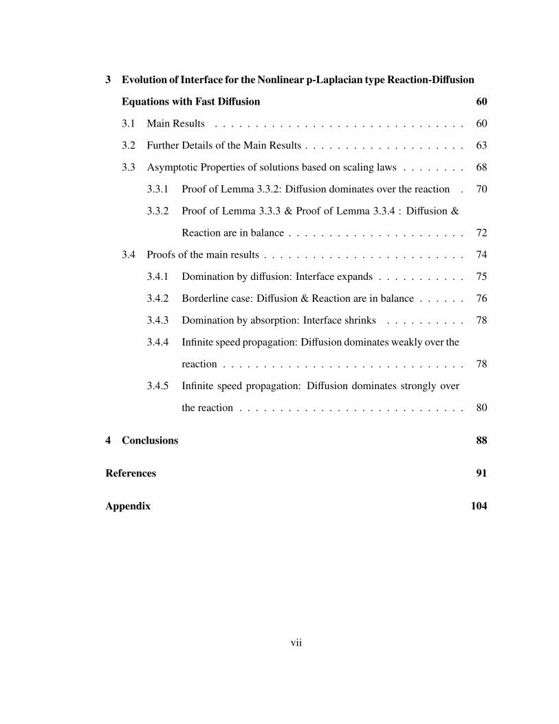
3 Evolution of Interface for the Nonlinear p-Laplacian type Reaction-Diffusion

Equations with Fast Diffusion 60

3.1 Main Results . . . . . . . . . . . . . . . . . . . . . . . . . . . . . . . 60

3.2 Further Details of the Main Results . . . . . . . . . . . . . . . . . . . . 63

3.3 Asymptotic Properties of solutions based on scaling laws . . . . . . . . 68

3.3.1 Proof of Lemma 3.3.2: Diffusion dominates over the reaction . 70

3.3.2 Proof of Lemma 3.3.3 & Proof of Lemma 3.3.4 : Diffusion &

Reaction are in balance . . . . . . . . . . . . . . . . . . . . . . 72

3.4 Proofs of the main results . . . . . . . . . . . . . . . . . . . . . . . . . 74

3.4.1 Domination by diffusion: Interface expands . . . . . . . . . . . 75

3.4.2 Borderline case: Diffusion & Reaction are in balance . . . . . . 76

3.4.3 Domination by absorption: Interface shrinks . . . . . . . . . . 78

3.4.4 Infinite speed propagation: Diffusion dominates weakly over the

reaction . . . . . . . . . . . . . . . . . . . . . . . . . . . . . . 78

3.4.5 Infinite speed propagation: Diffusion dominates strongly over

the reaction . . . . . . . . . . . . . . . . . . . . . . . . . . . . 80

4 Conclusions 88

References 91

Appendix 104

vii

List of Figures

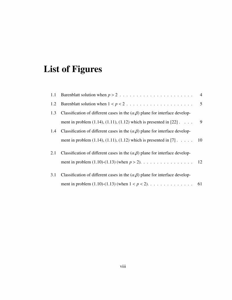
1.1 Barenblatt solution when p > 2 . . . . . . . . . . . . . . . . . . . . . . 4

1.2 Barenblatt solution when 1 < p < 2 . . . . . . . . . . . . . . . . . . . . 5

1.3 Classification of different cases in the (α,β) plane for interface develop-

ment in problem (1.14), (1.11), (1.12) which is presented in [22] . . . . 9

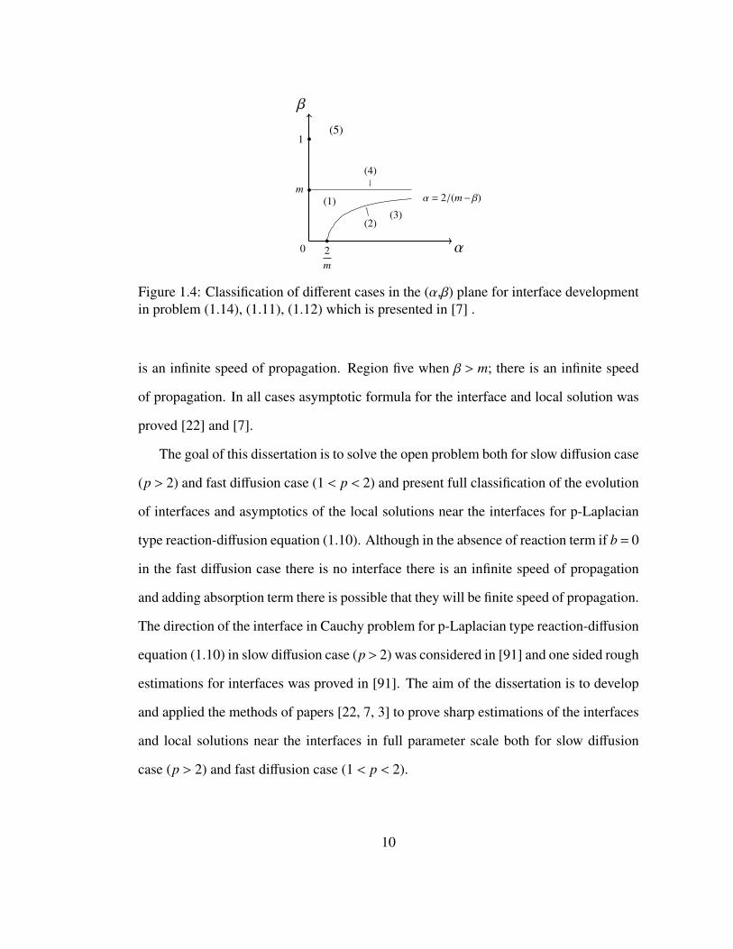
1.4 Classification of different cases in the (α,β) plane for interface develop-

ment in problem (1.14), (1.11), (1.12) which is presented in [7] . . . . . 10

2.1 Classification of different cases in the (α,β) plane for interface develop-

ment in problem (1.10)-(1.13) (when p > 2). . . . . . . . . . . . . . . . 12

3.1 Classification of different cases in the (α,β) plane for interface develop-

ment in problem (1.10)-(1.13) (when 1 < p < 2). . . . . . . . . . . . . . 61

viii

Acknowledgements

First of all, I would like to thanks and express my deepest appreciation to my degree

advisor Professor Dr. Ugur G. Abdulla, Ph.D., Dr. Sci., who has the attitude and the

substance of genius: he taught me well and has been kindly advising me until I became

a mathematician. I am so lucky to have him as a supervisor, without his guidance and

persistent help this dissertation would not have been possible.

I would like to extend my sincere thanks to the committee members Professor Dr.

Kanishka Perera, Ph.D., Professor Dr. Jay Kovats, Ph.D. and Professor Dr. Ming Zhang,

Ph.D. for their valuable guidance. I am grateful for their support.

I would also like to thanks all faculty members and staff in FIT who taught and

helped me.

ix

Dedication

I am very thankful to my parents; whose love and guidance are with me in whatever I

pursue. They are the ultimate role models. I wish to thank my supportive husband, and

my three wonderful children, Samar, Ali and Sama, who provide unending inspiration.

x

Chapter 1

Introduction

1.1 Physical Motivation

Consider the one-dimensional, turbulent, poly-tropic flow of a gas in a porous medium

[60].This flow can be mathematically described by the following laws.

• A poly-tropic equation of state

P = cγn (1.1)

where γ is a density of the gas, P is the pressure.

• The continuity equation

kγt + (γV)x = 0 (1.2)

where V is the velocity of the gas at the space point x at the time instant t.

• The flux under turbulent condition

γV = −M|Φx|p−2Φx (1.3)

1

where c,k,M are positive physical constants. n ≥ 1, p ≥ 3/2 and

Φ = P(n+1)/n. (1.4)

Combining (1.1)-(1.4), we get

kγt = Mc(p−1)(n+1)/n ∂

∂x

(∂(γn+1)∂x

p−2∂(γn+1)∂x

). (1.5)

Scaling the constants in (1.5) we obtain the nonlinear diffusion equation

ut =∂

∂x

(∂um

∂x

p−2∂um

∂x

)where m = n+ 1, m(p− 1) > 1. If m = 1, then we have non-Newtonian elastic filtration

equation

ut =∂

∂x

(∂u∂x

p−2∂u∂x

)where p > 1. The case p > 2 is called slow diffusion case and the case 1 < p < 2 is called

fast diffusion case [85]. In the case p = 2 we have a classical linear heat equation.

1.1.1 Instantaneous Point-Source Solution

The prelude of the mathematical theory of the nonlinear degenerate parabolic equations

is the papers [42, 105](see also [43]), where instantaneous point source type particular

solutions were constructed and analyzed. The property of finite speed of propagation

and the existence of compactly supported nonclassical solutions and interfaces became a

motivating force of the general theory. Consider the instantaneous point-source problem

2

for the nonlinear p-Laplacian equation

⎧⎪⎪⎪⎪⎪⎪⎪⎪⎪⎪⎪⎪⎪⎪⎪⎪⎨⎪⎪⎪⎪⎪⎪⎪⎪⎪⎪⎪⎪⎪⎪⎪⎪⎩

ut =(|ux|

p−2 ux)

x, x ∈ R, t > 0

u(x,0) = δ(x), x ∈ R∫R

u(x, t)dx = 1, t ≥ 0

u(x, t) ≥ 0

(1.6)

where δ(·) is Dirac’s point mass with support at the origin. The solution of this problem

(1.6) is given by

u∗(x, t) = t−1

2(p−1)C− k(p)

( |x|t1/2(p−1)

)p/(p−1) p−1p−2

where k(p) = p−2p (2(p − 1))−1/(p−1). In the slow diffusion case (p > 2) [42, 43]. In

the fast diffusion case (1 < p < 2), solution of this problem (1.6) has an infinite speed

of propagation. Meaning that the solution is instantaneously positive everywhere in

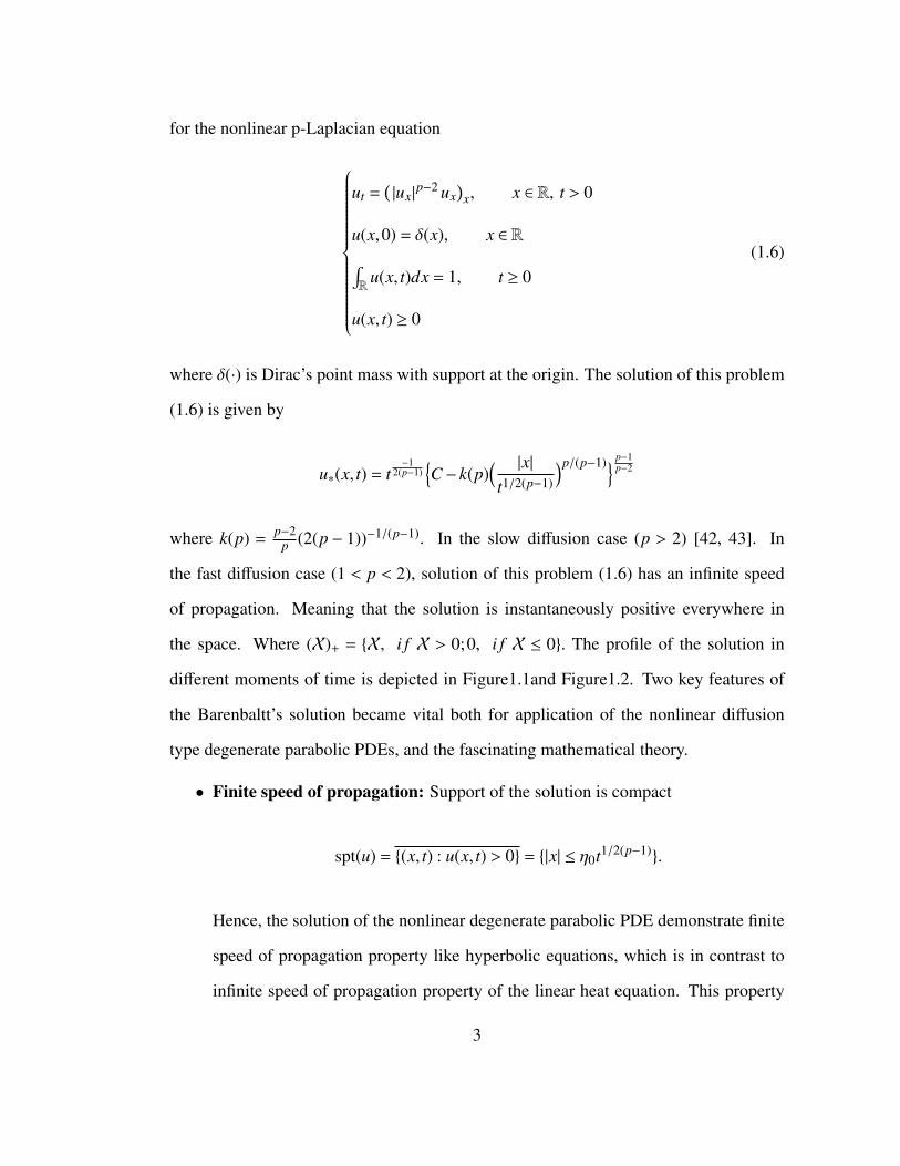
the space. Where (X)+ = X, i f X > 0;0, i f X ≤ 0. The profile of the solution in

different moments of time is depicted in Figure1.1and Figure1.2. Two key features of

the Barenbaltt’s solution became vital both for application of the nonlinear diffusion

type degenerate parabolic PDEs, and the fascinating mathematical theory.

• Finite speed of propagation: Support of the solution is compact

spt(u) = (x, t) : u(x, t) > 0 = |x| ≤ η0t1/2(p−1).

Hence, the solution of the nonlinear degenerate parabolic PDE demonstrate finite

speed of propagation property like hyperbolic equations, which is in contrast to

infinite speed of propagation property of the linear heat equation. This property

3

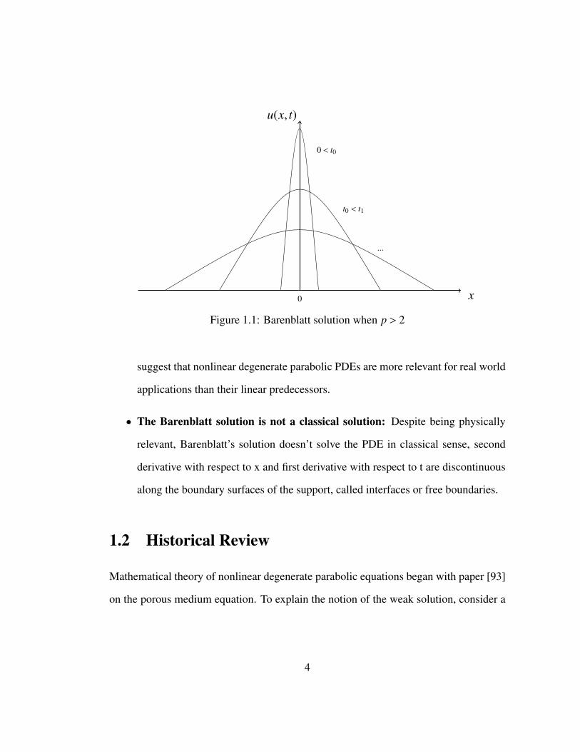
u(x, t)

x

0 < t0

t0 < t1

...

0

Figure 1.1: Barenblatt solution when p > 2

suggest that nonlinear degenerate parabolic PDEs are more relevant for real world

applications than their linear predecessors.

• The Barenblatt solution is not a classical solution: Despite being physically

relevant, Barenblatt’s solution doesn’t solve the PDE in classical sense, second

derivative with respect to x and first derivative with respect to t are discontinuous

along the boundary surfaces of the support, called interfaces or free boundaries.

1.2 Historical Review

Mathematical theory of nonlinear degenerate parabolic equations began with paper [93]

on the porous medium equation. To explain the notion of the weak solution, consider a

4

u(x, t)

0 < t0

t0 < t1

...

0x

Figure 1.2: Barenblatt solution when 1 < p < 2

Dirichlet problem for PDE

ut = um in Q = D× (0,T ] (1.7)

where D ⊂ RN be open domain, under the initial-boundary conditions

u(x,0) = u0(x), x ∈ Q (1.8)

u(x, t) = 0, (x, t) ∈ S = ∂D× (0,T ) (1.9)

Definition 1.2.1. We say that a non-negative function u = u(x, t) is a weak solution of

the Dirichlet problem(1.7)-(1.9) if

5

• um ∈ L2(0,T ; H10(D))

• u satisfies the integral identity

"QT

(∇um · ∇φ−uφt)dxdt =∫

Du0(x)φ(x,0)dx

for any φ ∈C1(QT ) satisfying φ(x,T ) = φ|S T = 0, where,

L2(0,T ; H10(D)) = u = u(t) : [0,T ]→ H1

0(D)

is a Hilbert space with the norm

||u||L2(0,T ;H1

0 (D)) = (∫ T

0||u||2

H10 (D)

dt)1/2=(∫ T

0

∫D

(|u|2+ |∇u|2)dxdt)1/2

In fact, instantaneous point-source solution is a weak solution in the sense of the

Definition 1.2.1. Currently there is a well established general theory of the nonlinear

degenerate parabolic equations (see [104, 58]). The questions of existence, uniqueness

of solutions to Cauchy problem and other initial-boundary value problems, comparison

theorems, regularity of weak solutions are analyzed in [19]-[105]. The general theory

of nonlinear degenerate second order parabolic PDEs in non-cylinrical non-smooth do-

mains was developed in [3, 14, 6, 12, 4]

1.3 Formulation of the open problems

We consider the Cauchy problem(CP) for the nonlinear degenerate parabolic equation:

Lu ≡ ut −(|ux|

p−2ux)

x+buβ = 0, x ∈ R,0 < t < T, (1.10)

6

with

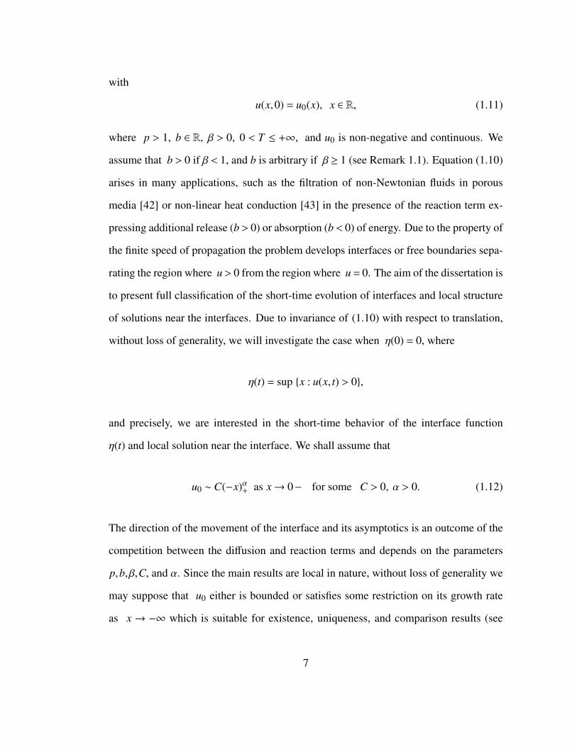
u(x,0) = u0(x), x ∈ R, (1.11)

where p > 1, b ∈ R, β > 0, 0 < T ≤ +∞, and u0 is non-negative and continuous. We

assume that b > 0 if β < 1, and b is arbitrary if β ≥ 1 (see Remark 1.1). Equation (1.10)

arises in many applications, such as the filtration of non-Newtonian fluids in porous

media [42] or non-linear heat conduction [43] in the presence of the reaction term ex-

pressing additional release (b> 0) or absorption (b< 0) of energy. Due to the property of

the finite speed of propagation the problem develops interfaces or free boundaries sepa-

rating the region where u> 0 from the region where u= 0. The aim of the dissertation is

to present full classification of the short-time evolution of interfaces and local structure

of solutions near the interfaces. Due to invariance of (1.10) with respect to translation,

without loss of generality, we will investigate the case when η(0) = 0, where

η(t) = sup x : u(x, t) > 0,

and precisely, we are interested in the short-time behavior of the interface function

η(t) and local solution near the interface. We shall assume that

u0 ∼C(−x)α+ as x→ 0− for some C > 0, α > 0. (1.12)

The direction of the movement of the interface and its asymptotics is an outcome of the

competition between the diffusion and reaction terms and depends on the parameters

p,b,β,C, and α. Since the main results are local in nature, without loss of generality we

may suppose that u0 either is bounded or satisfies some restriction on its growth rate

as x→ −∞ which is suitable for existence, uniqueness, and comparison results (see

7

Section 2.2). The special global case

u0(x) =C(−x)α+, x ∈ R, (1.13)

will be considered when the solution to the problem (1.10), (1.13) is of self-similar form.

Our estimations are global in time in these special cases.

Initial development of interfaces and structure of local solution near the interfaces is

very well understood in the case of the reaction-diffusion equations with porous medium

type diffusion term:

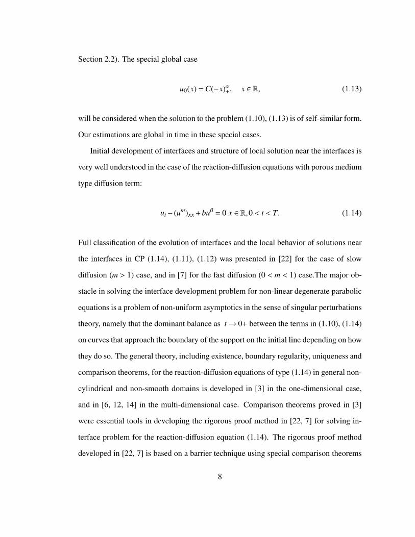
ut − (um)xx+buβ = 0 x ∈ R,0 < t < T. (1.14)

Full classification of the evolution of interfaces and the local behavior of solutions near

the interfaces in CP (1.14), (1.11), (1.12) was presented in [22] for the case of slow

diffusion (m > 1) case, and in [7] for the fast diffusion (0 < m < 1) case.The major ob-

stacle in solving the interface development problem for non-linear degenerate parabolic

equations is a problem of non-uniform asymptotics in the sense of singular perturbations

theory, namely that the dominant balance as t→ 0+ between the terms in (1.10), (1.14)

on curves that approach the boundary of the support on the initial line depending on how

they do so. The general theory, including existence, boundary regularity, uniqueness and

comparison theorems, for the reaction-diffusion equations of type (1.14) in general non-

cylindrical and non-smooth domains is developed in [3] in the one-dimensional case,

and in [6, 12, 14] in the multi-dimensional case. Comparison theorems proved in [3]

were essential tools in developing the rigorous proof method in [22, 7] for solving in-

terface problem for the reaction-diffusion equation (1.14). The rigorous proof method

developed in [22, 7] is based on a barrier technique using special comparison theorems

8

0

1

m

2m−1

β

α

α = 2/(m−β)

(1)

(2)

(3)

(4a)

(4b)

(4c)

(4d)

Figure 1.3: Classification of different cases in the (α,β) plane for interface developmentin problem (1.14), (1.11), (1.12) which is presented in [22] .

in irregular domains with characteristic boundary curves. Evolution of interfaces on lo-

cal solutions for reaction-diffusion (1.14) in the slow diffusion case was solved in [22]

and Figure 1.3 demonstrates the following classification:

Region one when α < 2/(m−min1,β); diffusion dominates and interface expands. Re-

gion two when α = 2/(m−β),0 < β < 1; diffusion and absorption are in balance in this

borderline case. There is a critical constant C∗ such that interface expands for C > C∗,

and shrinks for C < C∗. Region three when α > 2/(m− β),0 < β < 1; absorption term

dominates and interface shrinks. Region four when α ≥ 2/(m− 1),β ≥ 1; interface has

initial ’waiting time’.

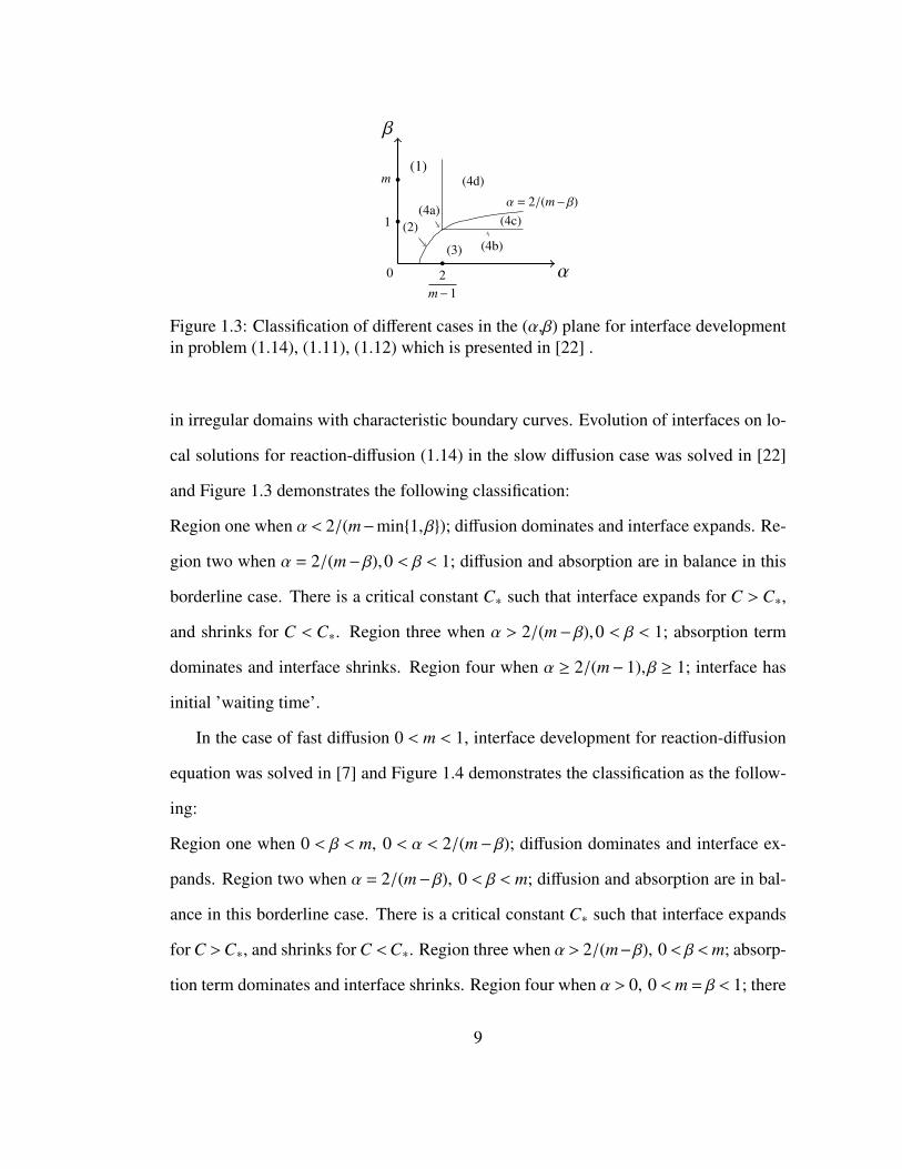
In the case of fast diffusion 0 < m < 1, interface development for reaction-diffusion

equation was solved in [7] and Figure 1.4 demonstrates the classification as the follow-

ing:

Region one when 0 < β < m, 0 < α < 2/(m− β); diffusion dominates and interface ex-

pands. Region two when α = 2/(m−β), 0 < β < m; diffusion and absorption are in bal-

ance in this borderline case. There is a critical constant C∗ such that interface expands

for C >C∗, and shrinks for C <C∗. Region three when α > 2/(m−β), 0 < β <m; absorp-

tion term dominates and interface shrinks. Region four when α > 0, 0 <m = β < 1; there

9

0

m

1

2m

β

α

α = 2/(m−β)

(5)

(1)

(2)(3)

(4)

Figure 1.4: Classification of different cases in the (α,β) plane for interface developmentin problem (1.14), (1.11), (1.12) which is presented in [7] .

is an infinite speed of propagation. Region five when β > m; there is an infinite speed

of propagation. In all cases asymptotic formula for the interface and local solution was

proved [22] and [7].

The goal of this dissertation is to solve the open problem both for slow diffusion case

(p > 2) and fast diffusion case (1 < p < 2) and present full classification of the evolution

of interfaces and asymptotics of the local solutions near the interfaces for p-Laplacian

type reaction-diffusion equation (1.10). Although in the absence of reaction term if b= 0

in the fast diffusion case there is no interface there is an infinite speed of propagation

and adding absorption term there is possible that they will be finite speed of propagation.

The direction of the interface in Cauchy problem for p-Laplacian type reaction-diffusion

equation (1.10) in slow diffusion case (p> 2) was considered in [91] and one sided rough

estimations for interfaces was proved in [91]. The aim of the dissertation is to develop

and applied the methods of papers [22, 7, 3] to prove sharp estimations of the interfaces

and local solutions near the interfaces in full parameter scale both for slow diffusion

case (p > 2) and fast diffusion case (1 < p < 2).

10

Chapter 2

Evolution of Interface for the

Nonlinear p-Laplacian type

Reaction-Diffusion Equations with

Slow Diffusion

In this chapter we present full classification of the evolution of interfaces and local struc-

ture of solution near the interfaces of the problem (1.10) -(1.13) in the slow diffusion

case (p > 2). The results of Chapter 2 are published in [20]

2.1 Description of Main Results

In Figure 2.1 we present classification diagram in (α,β)-plane for the initial interface

development in CP (1.10) -(1.12) if b > 0.

11

0

1

p−1

pp−2

β

α

α = p/(p−1−β)

(1)

(2)

(3)

(4a)

(4b)

(4c)

(4d)

Figure 2.1: Classification of different cases in the (α,β) plane for interface developmentin problem (1.10)-(1.13) (when p > 2).

• Region (1): α < p/(p−1−min1,β); diffusion dominates and interface expands.

• Region (2): α = p/(p− 1− β),0 < β < 1; diffusion and absorption are in balance

in this borderline case. There is a critical constant C∗ such that interface expands

for C >C∗, and shrinks for C <C∗.

• Region (3): α > p/(p−1−β),0 < β < 1; absorption term dominates and interface

shrinks.

• Region (4): α ≥ p/(p−2),β ≥ 1; interface has initial ’waiting time’.

To describe the asymptotic properties of the interface and local solution near the inter-

face, we divide the results into the two different subcases:

(I) b , 0 (either b > 0,β > 0 or b < 0,β ≥ 1) and p > 2; and (II) b = 0.

(I) In this case there are four different subcases, as shown in Figure 2.1 and itemized

above. (In view of our assumptions, the case b < 0 relates to the part of the (α,β) plane

with β ≥ 1.)

Region (1)

12

Theorem 2.1.1. Let u0 satisfies (1.12) with α < pp−1−min1,β . Then, interface initially

expands and

η(t) ∼ ξ∗t1/(p−α(p−2)) as t→ 0+, (2.1)

where

ξ∗ =Cp−2

p−α(p−2) ξ′∗ (2.2)

and ξ′∗ > 0 depends on p and α only (see Lemma 2.3.1). For arbitrary ρ < ξ∗ there

exists f (ρ) > 0 depending on C, p, and α such that

u(x, t) ∼ f (ρ)t(α/p−α(p−2)) as t→ 0+ (2.3)

along the curve x = ξρ(t) = ρt1/(p−α(p−2)).

A function f is a shape function of the self-similar solution of (1.10),(1.13) with b =

0 (see Lemma 2.3.1):

u∗(x, t) = tα

p−α(p−2) f (ξ), ξ = xt−1

p−α(p−2) , (2.4)

In fact, f is a unique solution of the following nonlinear ODE problem:

⎧⎪⎪⎪⎪⎪⎪⎨⎪⎪⎪⎪⎪⎪⎩(| f ′(ξ)|p−2 f ′(ξ)

)′+ 1

p−α(p−2)ξ f ′(ξ)− αp−α(p−2) f (ξ) = 0, −∞ < ξ < ξ∗

f (−∞) ∼C(−ξ)α, f (ξ∗) = 0, f (ξ) ≡ 0, ξ ≥ ξ∗.(2.5)

Its dependence on C is given through the following relation:

f (ρ) =Cp/(p−α(p−2)) f0(C(p−2)/(α(p−2)−p)ρ

), (2.6a)

13

f0(ρ) = w(ρ,1), ξ′∗ = supρ : f0(ρ) > 0 > 0, (2.6b)

where w is a solution of (1.10), (1.13) with b = 0,C = 1. Lower and upper estimations

for f are given in (2.31). Moreover,

ξ′∗ = Ap−2

p0

[ (p−1)p−1(p−α(p−2))(p−2)p−1

] 1p ξ′′∗ , (2.7)

where A0 = w(0,1) and ξ′′∗ is some number in [ξ1, ξ2], where

ξ1 = (p−1)1p(α(p−2)

)− 1p , ξ2 = 1 if (p−1)(p−2)−1 ≤ α < p(p−2)−1,

ξ1 = 1, ξ2 = (p−1)1p(α(p−2)

)− 1p , if 0 < α ≤ (p−1)(p−2)−1. (2.8)

In particular, if α = (p−1)(p−2)−1and p > 1+ (min1,β)−1, then the explicit solution

of the problem (1.10), (1.13) with b = 0 is given by (2.29), and we have

ξ1 = ξ2, ξ′∗ = (p−1)p−1(p−2)1−p, f0(x) =

(ξ′∗− x

)(p−1)/(p−2)+ . (2.9)

The explicit formulae (2.1) and (2.3) mean that the local behavior of the interface and

solution along x = ξρ(t) coincide with that of the problem (1.10), (1.13) with b = 0.

Region (2)

14

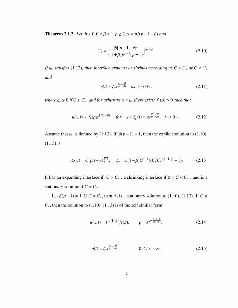
Theorem 2.1.2. Let b > 0,0 < β < 1, p ≥ 2,α = p/(p−1−β) and

C∗ =[ |b| |p−1−β|p

(1+β)pp−1(p−1)

] 1p−1−β . (2.10)

If u0 satisfies (1.12), then interface expands or shrinks according as C > C∗ or C < C∗

and

η(t) ∼ ζ∗tp−1−βp(1−β) as t→ 0+, (2.11)

where ζ∗ ≶ 0 if C ≶C∗, and for arbitrary ρ < ζ∗ there exists f1(ρ) > 0 such that

u(x, t) ∼ f1(ρ)t1/(1−β) for x = ζρ(t) = ρtp−1−βp(1−β) , t→ 0+ . (2.12)

Assume that u0 is defined by (1.13). If β(p−1) = 1, then the explicit solution to (1.10),

(1.13) is

u(x, t) =C(ζ∗t− x)1

1−β+ , ζ∗ = b(1−β)Cβ−1((C/C∗)p−1−β−1). (2.13)

It has an expanding interface if C > C∗ , a shrinking interface if 0 < C < C∗ , and is a

stationary solution if C =C∗.

Let β(p−1) , 1. If C = C∗, then u0 is a stationary solution to (1.10), (1.13). If C ,

C∗, then the solution to (1.10), (1.13) is of the self similar form:

u(x, t) = t1/(1−β) f1(ζ), ζ = xt−p−1−βp(1−β) , (2.14)

η(t) = ζ∗tp−1−βp(1−β) , 0 ≤ t < +∞. (2.15)

15

If C >C∗ then the interface expands, f1(0) = A1 > 0 (see Lemma 2.3.3), and

C1t1

1−β(ζ1− ζ

)µ+≤ u ≤C2t

11−β(ζ2− ζ

) pp−1−β

+, 0 ≤ x < +∞, 0 < t < +∞, (2.16)

where

µ = (p−1)(p−2)−1 if β(p−1) > 1; µ = p(p−1−β)−1 if β(p−1) < 1

which implies

ζ1 ≤ ζ∗ ≤ ζ2. (2.17)

The right-hand side of (2.16) ((2.17), respectively) may be replaced by C2t1

1−β (ζ2 −

ζ)p−1p−2+ (ζ2, respectively); see the Appendix Part A for the description of all the rele-

vant constants. Let β(p− 1) , 1 and 0 < C < C∗. Then, the interface shrinks and if

β(p−1) > 1, then [C1−β(−x)

p(1−β)p−1−β+ −b(1−β)t

] 11−β+ ≤ u

≤[C1−β(−x)

p(1−β)p−1−β+ −b(1−β)(1−

( CC∗

)p−1−β)t] 1

1−β+ , x ∈ R, 0 ≤ t < +∞, (2.18)

which again implies (2.17), where ζ1(ζ2, respectively) is replaced with

−C−p−1−β

p(b(1−β)

) p−1−βp(1−β)

(respectively,−C−

p−1−βp (b(1−β)

(1− (C/C∗)p−1−β) p−1−β

p(1−β)).

16

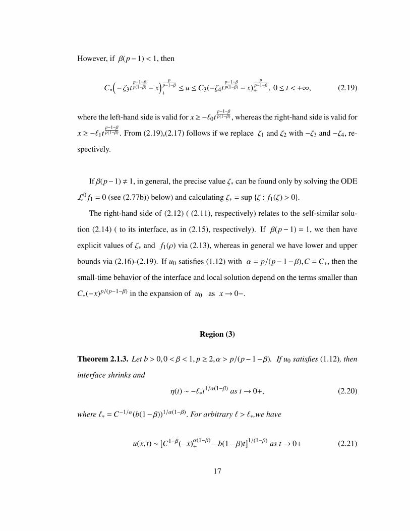
However, if β(p−1) < 1, then

C∗(− ζ3t

p−1−βp(1−β) − x

) pp−1−β

+≤ u ≤C3(−ζ4t

p−1−βp(1−β) − x)

pp−1−β+ , 0 ≤ t < +∞, (2.19)

where the left-hand side is valid for x≥−ℓ0tp−1−βp(1−β) ,whereas the right-hand side is valid for

x ≥ −ℓ1tp−1−βp(1−β) . From (2.19),(2.17) follows if we replace ζ1 and ζ2 with −ζ3 and −ζ4, re-

spectively.

If β(p−1) , 1, in general, the precise value ζ∗ can be found only by solving the ODE

L0 f1 = 0 (see (2.77b)) below) and calculating ζ∗ = sup ζ : f1(ζ) > 0.

The right-hand side of (2.12) ( (2.11), respectively) relates to the self-similar solu-

tion (2.14) ( to its interface, as in (2.15), respectively). If β(p− 1) = 1, we then have

explicit values of ζ∗ and f1(ρ) via (2.13), whereas in general we have lower and upper

bounds via (2.16)-(2.19). If u0 satisfies (1.12) with α = p/(p−1−β),C = C∗, then the

small-time behavior of the interface and local solution depend on the terms smaller than

C∗(−x)p/(p−1−β) in the expansion of u0 as x→ 0−.

Region (3)

Theorem 2.1.3. Let b > 0,0 < β < 1, p ≥ 2,α > p/(p−1−β). If u0 satisfies (1.12), then

interface shrinks and

η(t) ∼ −ℓ∗t1/α(1−β) as t→ 0+, (2.20)

where ℓ∗ =C−1/α(b(1−β))1/α(1−β). For arbitrary ℓ > ℓ∗,we have

u(x, t) ∼[C1−β(−x)α(1−β)

+ −b(1−β)t]1/(1−β) as t→ 0+ (2.21)

17

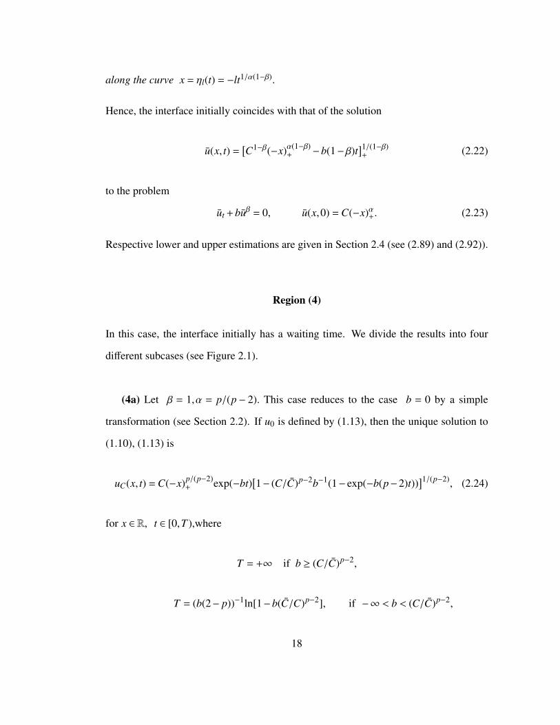
along the curve x = ηl(t) = −lt1/α(1−β).

Hence, the interface initially coincides with that of the solution

u(x, t) =[C1−β(−x)α(1−β)

+ −b(1−β)t]1/(1−β)+ (2.22)

to the problem

ut +buβ = 0, u(x,0) =C(−x)α+. (2.23)

Respective lower and upper estimations are given in Section 2.4 (see (2.89) and (2.92)).

Region (4)

In this case, the interface initially has a waiting time. We divide the results into four

different subcases (see Figure 2.1).

(4a) Let β = 1,α = p/(p− 2). This case reduces to the case b = 0 by a simple

transformation (see Section 2.2). If u0 is defined by (1.13), then the unique solution to

(1.10), (1.13) is

uC(x, t) =C(−x)p/(p−2)+ exp(−bt)

[1− (C/C)p−2b−1(1− exp(−b(p−2)t))

]1/(p−2), (2.24)

for x ∈ R, t ∈ [0,T ),where

T = +∞ if b ≥ (C/C)p−2,

T = (b(2− p))−1ln[1−b(C/C)p−2], if −∞ < b < (C/C)p−2,

18

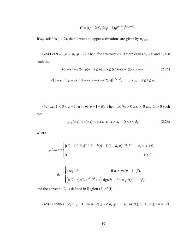
C =[(p−2)p/(2(p−1)pp−1)

]1/(p−2).

If u0 satisfies (1.12), then lower and upper estimations are given by uC±ϵ .

(4b) Let β = 1,α > p/(p−2). Then, for arbitrary ϵ > 0 there exists xϵ < 0 and δϵ > 0

such that

(C− ϵ)(−x)α+exp(−bt) ≤ u(x, t) ≤ (C+ ϵ)(−x)α+exp(−bt) (2.25)

×[1− ϵb−1(p−2)−p(1− exp(−b(p−2)t)

)]1/2−p, x > xϵ , 0 ≤ t ≤ δϵ .

(4c) Let 1 < β < p−1, α ≥ p/(p−1−β). Then, for ∀ϵ > 0 ∃xϵ < 0 and δϵ > 0 such

that

g−ϵ(x, t) ≤ u(x, t) ≤ gϵ(x, t), x ≥ xϵ , 0 ≤ t ≤ δϵ , (2.26)

where

gϵ(x, t) =

⎧⎪⎪⎪⎪⎪⎪⎨⎪⎪⎪⎪⎪⎪⎩[(C+ ϵ)1−β|x|α(1−β)+b(β−1)(1−dϵ)t]1/(1−β), xϵ ≤ x < 0,

0, x ≥ 0,

dϵ =

⎧⎪⎪⎪⎪⎪⎪⎨⎪⎪⎪⎪⎪⎪⎩ϵ sign b if α > p/(p−1−β),((

(C+ ϵ)/C∗)p−1−β

+ ϵ)

sign b if α = p/(p−1−β),

and the constant C∗ is defined in Region (2) of (I).

(4d) Let either 1<β< p−1, p/(p−2)≤α< p/(p−1−β), or β≥ p−1, α≥ p/(p−2).

19

If α = p/(p−2) then for arbitrary ϵ > 0 there exists xϵ < 0 and δϵ > 0 such that

(C− ϵ)(−x)p/(p−2)+ (1−γ−ϵ t)1/(2−p) ≤ u ≤ (C+ ϵ)(−x)p/(p−2)

+ (1−γϵ t)1/(2−p), (2.27)

where

γϵ =[2(p−1)pp−1(C+ ϵ)p−2/(p−2)1−p]+ ϵ.

However, if α > p/(p− 2), then for arbitrary ϵ > 0 there exists xϵ < 0 and δϵ > 0 such

that

(C− ϵ)(−x)α+ ≤ u ≤ (C+ ϵ)(−x)α+(1− ϵt)1/2−p), x ≥ xϵ , 0 ≤ t ≤ δϵ . (2.28)

(II) b = 0. We divide this case into three subcases.

(1) Let p > 2, 0 < α < p/(p− 2). In this case, the interface expands. First, assume

that u0 is defined by (1.13). Then, if α = (p− 1)/(p− 2), the explicit solution to the

problem (1.10), (1.13) is

u(x, t) =C(ξ∗t− x)(p−1)/(p−2)+ , ξ∗ =Cp−2

( p−1p−2

)p−1. (2.29)

If 0 < α < p/(p−2), then the solution to (1.10), (1.13) has the self-similar form (2.4)

η(t) = ξ∗t1

p−α(p−2) , 0 ≤ t < +∞, (2.30)

where ξ∗ and f satisfy (2.2), (2.5)-(2.8). Moreover, we have

C4tα

p−α(p−2) (ξ3− ξ)p−1p−2+ ≤ u ≤C5t

αp−α(p−2) (ξ4− ξ)

p−1p−2+ , (2.31)

20

0 ≤ x < +∞, 0 < t < +∞,

where ξ3 (ξ4, respectively) is defined by the right-hand side of (2.7), where we replace

ξ′′∗ with Cp−2

p−α(p−2) ξ1 ( with Cp−2

p−α(p−2) ξ2, respectively) and

C4 =Cp/(p−α(p−2))A0ξ(p−1)/(2−p)3 , C5 =Cp/(p−α(p−2))A0ξ

−(p−1)/(p−2)4 .

In the particular case α = (p−1)(p−2)−1, when an explicit solution is given by (2.29),

we have ξ3 = ξ4 = ξ∗ and both lower and upper estimations in (2.31) lead to the explicit

solution (2.29). In general, when α , (p−1)(p−2)−1 the precise value ξ∗ relates to the

similarity ODE for f (ξ) from (2.5), namely, ξ∗ = supξ : f (ξ) > 0. If u0 satsfies (1.12)

with (0 < α < p/(p−2)), then (2.1) and (2.3) are valid. Lower and upper bounds for f (ρ)

follow from (2.31).

(2) Let p > 2,α = p/(p−2). In this case, the interface initially has a waiting time. If

u0 is defined by (1.13), then the explicit solution to (1.10), (1.13) is

uC(x, t) =C(−x)α+[1− (C/C)p−2(p−2)t

]1/(2−p) x ∈ R, 0 ≤ t < T, (2.32)

where

T = (C/C)p−2(p−2)−1

and the constant C is defined in Region (4) of (I).

If u0 satisfies (1.12) with α = p/(p−2), then lower and upper estimations are given by

uC±ϵ .

(3) Let p> 2,α > p/(p−2). In this case also the interface initially remains stationary

21

and for arbitrary ϵ > 0 there exists xϵ < 0 and δϵ > 0 such that

(C− ϵ)(−x)α+ ≤ u ≤ (C+ ϵ)(−x)α+(1− ϵt)1/2−p), xϵ ≤ x, 0 ≤ t ≤ δϵ . (2.33)

Remark 1.1. We are not interested in the special case p= 2 of semi-linear heat equation.

This case was completed in [74, 75] (see also [22]). However, we will mention when

our results extend to the limit case p = 2. In general, the case p = 2 is in some sense a

singular limit. For example, if b > 0,0 < β < 1, p− 1 > β,α < pp−1−β , then the interface

initially expands and if p > 2, then we prove in this chapter that

η(t) ∼C1t1/(p−α(p−2)) as t→ 0+,

while if 1 < p < 2, we prove in Chapter 3 that

η(t) ∼C2t(p−1−β)/p(1−β) as t→ 0+ .

Formally, as p→ 2 both estimates yield a false result, and from [75] it follows that if

p = 2, then

η(t) ∼C3(t log 1/t)12

(Ci, i = 1,3 are positive constants).

2.2 Preliminary results

The mathematical theory of non-linear p-Laplacian type degenerate parabolic equations

is well developed. We shall follow the definition of weak solutions and of supersolutions

(or subsolutions) of the equation (1.10) in the following sense:

22

Definition 2.2.1. A measurable function u≥ 0 is a local weak solution (respectively sub-

or supersolution) of (1.10) in R× (0,T ] if

• u ∈Cloc(0,T ; L2loc(R)∩Lp

loc(0,T ;W1,ploc (R)∩L1+β

loc (R));

• For ∀ subinterval [t0, t1] ⊂ (0,T ] and for ∀µi ∈ C1[t0, t1], i = 1,2 such that µ1(t) <

µ2(t) for t ∈ [t0, t1]

∫ µ2(t)

µ1(t)uφdx

t1t0+

∫ t1

t0

∫ µ2(t)

µ1(t)(−uφt + |ux|

p−2uxφx+buβφ)dxdt = 0 (resp. ≤ or ≥ 0),

(2.34)

where φ ∈C2,1x,t (D) is an arbitrary function that equals zero when x = µi(t), t0 ≤ t ≤

t1, i = 1,2, and

D = (x, t) : µ1(t) < x < µ2(t), t0 < t < t1.

The questions of existence and uniqueness of initial boundary value problems for

(1.10), comparison theorems, and regularity of weak solutions are known due to [58,

57, 59, 53, 60, 82, 83, 99] etc. Qualitative properties of free boundaries for the quasi-

linear degenerate parabolic equations were studied via energy methods in [38]. The

proof of the following typical comparison result is standard.

Lemma 2.2.2. Let g be a non-negative and continuous function in Q, where

Q = (x, t) : η0(t) < x < +∞,0 < t < T ≤ +∞,

f is in C2,1x,t in Q outside a finite number of curves x = η j(t), which divide Q into a finite

number of subdomains Q j, where η j ∈ C[0,T ]; for arbitrary δ > 0 and finite ∆ ∈ (δ,T ]

23

the function η j is absolutely continuous in [δ,∆]. Let g satisfy the inequality

Lg ≡ gt −(|gx|

p−2gx)

x+bgβ ≥ 0, (≤ 0)

at the points of Q, where g ∈C2,1x,t . Assume also that the function |gx|

p−2gx is continuous

in Q and g ∈ L∞(Q∩ (t ≤ T1)) for any finite T1 ∈ (0,T ]. Then, g is a supersolution

(subsolution) of (1.10). If, in addition we have

gx=η0(t)

≥ (≤) ux=η0(t)

, gt=0≥ (≤) u

t=0,

then

g ≥ (≤) u, in Q.

Suppose that b ≥ 0 and that u0 may have unbounded growth as |x| → +∞. It is

well known that in this case some restriction must be imposed on the growth rate for

existence, uniqueness and comparison results in the CP (1.10), (1.11). Optimal growth

condition for the equation (1.10) with b = 0, p > 2 was derived in [57, 59]. If initial data

may be majorised by power law function (1.13), then there exists a unique solution (with

T = +∞) and a comparison principle is valid if 0 < α < p/(p− 2). If α = p/(p− 2),

then existence, uniqueness, and comparison results are valid only locally in time. In

particular, from [57, 59] it follows that the unique explicit solution to (1.10), (1.13) with

b = 0,α = p/(p−2),T = (C/C)p−2(p−2)−1 is uC(x, t) from (2.32).

If the function u(x, t) is a solution to CP (1.10), (1.13) with b = 0, then the function

u(x, t) = exp(−bt)u(x, (b(2− p))−1(exp(b(2− p)t)−1))

is a solution to (1.10) with b , 0,β = 1. Hence, from the above mentioned result it

24

follows that the unique solution to CP (1.10), (1.13) with p> 2,b, 0,β= 1,α= p/(p−2)

is the function uC(x, t) from (2.24).

It is proved in [53] that existence, uniqueness and comparison theorems are valid for

the CP (1.10),(1.11) with b = 0, 1 < p < 2 without any growth condition on the initial

function u0 at infinity. In particular, α > 0 is arbitrary in (1.13).

We are not interested in necessary and sufficient conditions on the growth rate at

infinity for existence, uniqueness, and comparison results for the CP (1.10), (1.11) with

b > 0, p > 2,β > 0; for our purposes, it is enough to mention that if u0 may be majorised

by the function (1.13) with α satisfying 0 < α < p/(p− 2), then the CP (1.10), (1.11)

with b > 0, p > 2,β > 0,T = +∞ has a unique solution and for this class of initial data

a comparison principle is valid. This easily follows from the fact that the solution of

the CP (1.10), (1.11) with b = 0 is a supersolution of the CP with b > 0, and hence it

becomes a global locally bounded uniform upper bound for the increasing sequence of

approximating bounded solutions of the CP with b > 0. Similarly, if b > 0,1 < p < 2 due

to above mentioned result of [53], existence, uniqueness and comparison theorems are

valid for the CP (1.10),(1.11), and for the respective boundary value problems without

any growth condition on the continuous initial function at infinity. In particular, α > 0

could be arbitrary in (1.13).

2.2.1 Traveling wave solutions

Traveling wave solution for equation(1.10) is investigated in [91]. We consider the

parabolic p-Laplacian equation with strong absorption (1.10) with p > 2, 0 < β < 1, b >

0, x ∈ R, t ≥ 0 and equation (1.11), where u0(x) is a continuous and non-negative func-

tion with compact support. We seek solutions of the form:

u(x, t) = φ((kt− x)),

25

such that 0 , k ∈ R, φ(η) ≥ 0, φ . 0, and φ→ 0 as η→ −∞. In the case φ(η) = 0 for

η ≤ η0 ∈ R. Without loss of generality we can assume that η0 = 0. Plugging u(x, t) =

φ((kt− x)) into (1.10), we have

⎧⎪⎪⎪⎪⎪⎪⎨⎪⎪⎪⎪⎪⎪⎩(|φ′|p−2φ′)′− kφ′−bφβ = 0, φ = φ(η), η > 0,

φ(0) = φ′(0) = 0.(2.35)

If we can find a positive solution, φ, to the problem above in R+, then (1.10) ad-

mits a finite traveling-wave solution. Note that the solution to the problem (2.35) is

understood in the weak sense. In [91] it is proven that there exists a unique posi-

tive and monotonically increasing solution φ(η) : R+ → R+ of the problem (2.35) with

k , 0, p > 2,b > 0,0 < β < 1. By introducing the variables

X = φ, Y = (φ′)p−1

the problem can be reformulated as finding the nontrivial trajectories of the dynamical

system

X′ = φ′ = Y1/(p−1), Y′ = ((φ′)p−1)′ = (|φ′|p−2φ′)′ = kφ′+bφβ = kY1/(p−1)+bXβ

which start from (0,0) at η = 0, and stay in the first quadrant Ω1 = (X,Y) : X > 0, Y > 0

for 0 < η < +∞. We write the system as an O.D.E problem

⎧⎪⎪⎪⎪⎪⎪⎨⎪⎪⎪⎪⎪⎪⎩dYdX = f (X,Y) = k+bXβY−

1p−1 ,

Y(0) = 0.(2.36)

26

The problem (2.36) has a unique global solution [91]. Having global solution Y , con-

sider the problem ⎧⎪⎪⎪⎪⎪⎪⎨⎪⎪⎪⎪⎪⎪⎩dφdη = Y1/(p−1)(φ(η)),φ(0) = 0.

(2.37)

There exists a unique maximal solution defined in (−∞,β′) such that

limη→β′−

φ(η) = +∞

if β′ is finite. In fact, it easily follows from (2.37) that the same is true if β′ = +∞ [91].

It follows that the solution of (2.37) defined in (−∞,β′) and satisfies

⎧⎪⎪⎪⎪⎪⎪⎨⎪⎪⎪⎪⎪⎪⎩(|φ′|p−2φ′)′− kφ′−λφq = 0 in (−∞,β′),

φ(0) = 0, φ′(0) = 0.

(2.38)

It remains to prove that β′ = +∞. In [91] it is demonstrated that this follows from the

following lemma on the asymptotic properties of the solution to the problem (2.36).

Lemma 2.2.3. [91] Let Y be a solution of (2.36). Then we have

(i) Y(X) ∼ [ bp(p−1)(β+1) ]

(p−1)/pX(p−1)(β+1)

p as X→ +∞ if β(p−1) > 1;

(ii) Y(X) ∼ [ p(p−1)(β+1) ]

(p−1)/pX(p−1)(β+1)

p as X→ 0 if β(p−1) < 1;

(iii) Y(X) ∼ kX as X→ +∞ if k > 0, β(p−1) < 1;

(iv) Y(X) ∼ kX as X→ 0 if k > 0, (p−1)β > 1;

(v) Y(X) ∼ (− kb )1−pXβ(p−1) as X→ +∞ if k < 0, β(p−1) < 1;

(vi) Y(X) ∼ (− kb )1−pXβ(p−1) as X→ 0 if k < 0, β(p−1) > 1.

In particular, Lemma 2.2.3 is equivalent to the following key lemma on the asymp-

27

totic properties of the traveling wave solutions of the PDE (1.10).

Lemma 2.2.4. [91] The equation (1.10) admits a finite traveling-wave solution u(x, t) =

φ(kt− x) with φ(0) = 0 if k , 0. Moreover,

(i) limη→+∞ η−

pp−1−βφ(η) =

[ b(p−1−β)p

pp−1(p−1)(β+1)]1/(p−1−β) if β(p−1) > 1;

(ii) limη→0 η−

pp−1−βφ(η) =

[ b(p−1−β)p

pp−1(p−1)(β+1)]1/(p−1−β) if β(p−1) < 1;

(iii) limη→+∞ η−

p−1p−2φ(η) =

( p−2p−1) p−1

p−2 k1/(p−2) if k > 0, β(p−1) < 1;

(iv) limη→0 η−

p−1p−2φ(η) =

( p−2p−1) p−1

p−2 k1/(p−2) if k > 0, β(p−1) > 1;

(v) limη→+∞ η− 1

1−βφ(η) =[(1−β)

(− b

k)] 1

1−β if k < 0, β(p−1) < 1;

(vi) limη→0 η− 1

1−βφ(η) =[(1−β)

(− b

k)] 1

1−β if k < 0, β(p−1) > 1.

Both Lemma 2.2.3 and Lemma 2.2.4 were proved in [91]. Below we sketch simple

proof of the Lemma 2.2.3 based on the scaling method.

Proof of Lemma 2.2.3. • proof of (i): Consider equation (2.36). Rescaled solution

Ym(X) = mY(mγX), Y(X) = m−1Ym(m−γX) (2.39)

with γ = −p(p−1)(β+1) satisfies

⎧⎪⎪⎪⎪⎪⎪⎨⎪⎪⎪⎪⎪⎪⎩dYmdX = m

β(p−1)−1(p−1)(β+1) k+bXβY

− 1p−1

m , 0 < X < +∞,

Ym(0) = 0.

(2.40)

One can easily prove that the sequence Ym is uniformly bounded, and mono-

tonically decreasing if k > 0, and monotonically increasing if k < 0. Therefore,

limm→0

Ym(X) = Y(X) (2.41)

28

exists. Since β(p− 1) > 1, passing to the limit as m → 0 from (2.40) it easily

follows that Y satisfies the ODE problem

dYdX= bXβY−

1p−1 ,0 < X < +∞; Y(0) = 0,

that is to say

Y(X) =[ bp(β+1)(p−1)

] p−1p X

(p−1)(β+1)p .

Changing variable in (2.41) as Z = mγX, we easily deduce claim (i) in Lemma

2.2.3.

• proof of (ii): Since β(p− 1) < 1, the exponent of m in (2.40) is negative. In a

similar way one can prove that the limit

limm→+∞

Ym(X) =[ bp(β+1)(p−1)

] p−1p X

(p−1)(β+1)p (2.42)

exists. By changing variable in (2.42), claim (ii) follows.

• proof of (iii): Rescaled solution of (2.36)

Ym = mY(m−1X)

satisfies ⎧⎪⎪⎪⎪⎪⎪⎨⎪⎪⎪⎪⎪⎪⎩dYmdX = k+m

1−β(p−1)p−1 bXβY

− 1p−1

m , 0 < X < +∞,

Ym(0) = 0.(2.43)

Standard comparison lemma implies that

Ym(X) ≥ kX, 0 < X < +∞. (2.44)

29

Similarly, as in the case (i), it is proved that the sequence Ym is uniformly

bounded and equicontinuous on compact subsets of (0,+∞) as m→ 0. Arzela-

Ascoli theorem implies the existence of the convergent subsequence of Ym on

every compact subset of R+. By selecting expanding sequence of compact sub-

sets and Cantor’s diagonalization one can deduce the existence of the limit

limm′→0

Ym′(X) = kX, 0 < X < +∞,

for some subsequence m′, and convergence being uniform on compact subsets.

By changing the variable under the limit sign, the claim (iii) follows. The proof

of (iv) is similar as the proof of (iii).

• proof of (v) and (vi) can be pursued similarly by rescaling solution of (2.36) as

Ym = mY(m−1

β(p−1) X)

which solves the problem

⎧⎪⎪⎪⎪⎪⎪⎨⎪⎪⎪⎪⎪⎪⎩m

1−β(p−1)β(p−1) dYm

dX = k+bXβY− 1

p−1m , 0 < X < +∞,

Ym(0) = 0.

(2.45)

Similar analysis as in the case (iii) implies the limit relation

limm→0

Ym =(−k

b

)1−pXβ(p−1),0 < X < +∞

By changing variable under the limit sign, claim (v) follows. The proof of (vi) is

similar.

30

2.3 Asymptotic Properties of solutions based on scaling

laws

In the next four lemmas, we apply rescaling to establish some preliminary estimations

of the solution to CP.

Lemma 2.3.1. If b = 0 and p > 2,0 < α < p/(p−2), then the solution u of the CP (1.10),

(1.13) has a self-similar form (2.4), where the self-similarity function f satisfies (2.6).

If u0 satisfies (1.12), then the solution to CP (1.10), (1.11) satisfies (2.1)-(2.3)

Lemma 2.3.2. Let u be a solution to the CP(1.10), (1.11) and u0 satisfy (1.12). Let one

of the following conditions be valid:

(a) b > 0, 0 < β < 1 < p, 0 < α < p/(p−1−β);

(b) b , 0, β ≥ 1, p > 2, 0 < α < p/(p−2).

Then, u satisfies (2.3).

Lemma 2.3.3. Let u be a solution to the CP(1.10), (1.13) with b > 0, 0 < β < 1, p >

2, α = p/(p − 1 − β). Then, the solution u has the self-similar form (2.14). If C >

C∗, then f1(0)= A1, where A1 is a positive number depending on p,β,C, and b. If u0 sat-

isfies (1.12) with α = p/(p−1−β),C >C∗, then u satisfies

u(0, t) ∼ A1t1/(1−β) as t→ 0+ . (2.46)

Lemma 2.3.4. Let u be a solution to the CP (1.10)-(1.12) with b > 0,0 < β < 1,α >

p/(p− 1− β). Then, for arbitrary ℓ > ℓ∗ (see (2.20)) the asymptotic formula (2.21) is

valid with x = ηℓ(t) = −ℓt1/α(1−β).

31

2.3.1 Proof of Lemma 2.3.1 & Lemma 2.3.2: Diffusion dominates

over the reaction

Proof of Lemma 2.3.1. If we consider a function

uk(x, t) = ku(k−1α x,k

α(p−2)−pα t) k > 0,

it may easily be checked that this satisfies (1.10), (1.13). From [57, 59], it follows that

under the condition of the lemma there exists a unique global solution to (1.10), (1.13).

Therefore, we have

u(x, t) = ku(k−1/αx,k(α(p−2)−p)/α), k > 0. (2.47)

If we choose k = tα/(p−α(p−2)), then (2.47) implies (2.4) for u with f (ξ)= u(ξ,1). In fact, f

is a unique non-negative and differentiable weak solution of the boundary value problem

(2.5) and there exists an ξ∗ > 0 such that f satisfies (2.5): it is positive and smooth

for ξ < ξ∗ and f = 0 for ξ ≥ ξ∗([42]). Thus, (2.30) is valid. To find the dependence

of f on C, we can again use scaling. Let

v(x, t) =C−1u(x, t).

Plugging it into (1.10) with b = 0 such that

vt(x, t) =C−1ut(x, t)

(|vx(x, t)|p−2vx(x, t)

)x=C1−p

(|ux(x, t)|p−2ux(x, t)

)x.

32

We have ⎧⎪⎪⎪⎪⎪⎪⎨⎪⎪⎪⎪⎪⎪⎩C2−pvt(x, t) =

(|vx(x, t)|p−2vx(x, t)

)x; x ∈ R, t > 0

v(x,0) =C−1u(x,0) =C−1C(−x)α+ = (−x)α+; x ∈ R.

Choose time variable τ =Cp−2t, we have

w(x, τ) = v(x,c2−pτ)

which solves CP (1.10), (1.13) with C = 1. Then, it may be easily checked that for

arbitrary k > 0

u(x, t) = kw(C1/αk−1/αx,Cp/αk(α(p−2)−p)/αt).

By choosing k = (Cp/αt)α/(p−α(p−2)), we then have

u(x, t) =Cp

p−α(p−2) w(Cp−2

α(p−2)−p ξ,1)tα/(p−α(p−2)). (2.48)

Formulae (2.6) and (2.2) follow from (2.48) and (2.4).

Now assume that u0 satisfies (1.12). Then, for arbitrary sufficiently small ϵ > 0 there

exists xϵ < 0, such that

(C− ϵ/2)(−x)α+ ≤ u0(x) ≤ (C+ ϵ/2)(−x)α+, x ≥ xϵ . (2.49)

Let uϵ(x, t) (u−ϵ(x, t), respectively) be a solution to the CP (1.10), (1.11) with initial

data (C+ϵ)(−x)α+ ((C−ϵ)(−x)α+, respectively). Since the solution to the CP (1.10), (1.11)

is continuous, there exists a number δ = δ(ϵ) > 0 such that

uϵ(xϵ , t) ≥ u(xϵ , t), u−ϵ(xϵ , t) ≤ u(xϵ , t) for 0 ≤ t ≤ δ. (2.50)

33

From (2.49), (2.50), and a comparison principle, it follows that

u−ϵ ≤ u ≤ uϵ for x ≥ xϵ , 0 ≤ t ≤ δ. (2.51)

Obviously

u±ϵ(ξρ(t), t) = f (ρ;C± ϵ)tα/(p−α(p−2)), t ≥ 0. (2.52)

(Furthermore, we denote the right-hand side of(2.6a) by f (ρ,C).) Now taking x= ξρ(t) in

(2.51), after multiplying to t−α/(p−α(p−2)) and passing to the limit, first as t→ 0 and then

as ϵ → 0, we can easily derive (2.3). Similarly, from (2.51), (2.30), and (2.2), (2.1)

easily follows.

Proof of Lemma 2.3.2. As in the previous proof, (2.49)-(2.51) follow from (1.12). Let

the conditions of one of the cases (a) or (b) with b > 0 be valid. Then, from the results

mentioned earlier it follows that the existence, uniqueness, and comparison results of

the CP (1.10), (1.11) with u0 = (C± ϵ)(−x)α+, T = +∞ hold. Now, if we rescale

u±ϵk (x, t) = ku±ϵ(k−1/αx,k(α(p−2)−p)/αt

), k > 0, (2.53)

then u±ϵk (x, t) satisfies the following problem:

ut − (|ux|p−2ux)x+bk(α(p−1−β)−p)/αuβ = 0, x ∈ R, t > 0, (2.54a)

u(x,0) = (C± ϵ)(−x)α+, x ∈ R. (2.54b)

There exists a unique solution to CP (2.54), which also obeys a comparison principle.

Since α(p− 1− β)− p < 0, by using a comparison principle in Lemma 2.3.1 it follows

34

that

u±ϵk1(x, t) ≤ u±ϵk2

(x, t) ≤ · · · ≤ v±(x, t), x ∈ R, t ≥ 0; if k1 < k2, (2.55)

where v±ϵ is a solution to CP (1.10), (1.11) with b= 0, u0 = (C±ϵ)(−x)α+, T =+∞. From

the results of [57, 99], it follows that the sequence of non-negative and locally bounded

solutions u±ϵk is locally uniformly Holder continuous, and weakly pre-compact in

W1,ploc (R× (0,T )). Since α(p− 1− β)− p < 0, passing to limit as k→ +∞, from (2.34)

it follows that the limit function is a solution of the CP (1.10), (1.11) with b = 0, u0 =

(C± ϵ)(−x)α+, T = +∞. Due to uniqueness we have

limk→+∞

u±ϵk (x, t) = v±(x, t), x ∈ R, t ≥ 0. (2.56)

Hence, v±ϵ satisfies (2.52). If we now take x= ξρ(t),where ρ is an arbitrary fixed number

satisfying ρ < ξ∗, then from (2.56) it follows that

limk→+∞

ku±ϵ(k−1/αξρ(t),k(α(p−2)−p)/αt

)= f (ρ;C± ϵ)tα(p−α(p−2)), t > 0. (2.57)

If we take τ = k(α(p−2)−p)/αt, then (2.57) implies

u±ϵ(ξρ(τ), τ) ∼ f (ρ;C± ϵ)τα(p−α(p−2)), as τ→ 0+ . (2.58)

As before, (2.3) follows from (2.51), (2.58).

Now consider the case (b) with b < 0. Suppose that u±ϵ is a solution of the Dirichlet

problem

ut − (|ux|p−2ux)x+buβ = 0, |x| < |xϵ |, 0 < t < δ, (2.59a)

35

u(x,0) = (C± ϵ)(−x)α+, |x| ≤ |xϵ |, (2.59b)

u(xϵ , t) = (C± ϵ)(−xϵ)α, u(−xϵ , t) = 0, 0 ≤ t ≤ δ. (2.59c)

The function u±ϵk is defined as in (2.53), satisfies the Dirichlet problem:

ut − (|ux|p−2ux)x+bk(α(p−1−β)−p)/αuβ = 0 in Dk

ϵ , (2.60a)

u(k1/αxϵ , t) = k(C± ϵ)(−xϵ)α, u(−k1/αxϵ , t) = 0, 0 ≤ t ≤ k(p−α(p−2))/αδ (2.60b)

u(x,0) = (C± ϵ)(−x)α+, |x| ≤ k1/α|xϵ |, (2.60c)

where

Dkϵ = (x, t) : |x| < k1/α|xϵ |, 0 < t ≤ k(p−α(p−2))/αδ.

There exists a number δ > 0 (which does not depend on k) such that both (2.59a)-(2.59c)

and (2.60a)-(2.60c) have a unique solution (see discussion preceding Lemma 2.3.1). In

view of finite speed of propagation, δ = δ(ϵ) > 0 may be chosen such that

u(−xϵ , t) = 0, 0 ≤ t ≤ δ. (2.61)

Applying the comparison theorem, from (2.49), (2.50) and (2.61),(2.51) follows for |x| ≤

|xϵ |, 0 ≤ t ≤ δ.

36

To prove the convergence of the sequences u±ϵk as k → +∞, we need to prove

uniform boundedness. Consider a function

g(x, t) = (C+1)(1+ x2)α2 (1− νt)

12−p , x ∈ R, 0 ≤ t ≤ t0 =

ν−1

2,

where

ν = h∗+1, h∗ = h∗(α; p) =maxx∈R

h(x), (2.62)

h(x) = (p−2)αp−1(C+1)p−2(1+ x2)(α−2)(p−1)−2−α

2 x2|x|p−2

×(1+ x2

x2 + (p−2)1+ x2

|x|2+ (α−2)(p−1)

).

Then, we have

Lkg ≡ gt −(|gx|

p−2gx)

x+bkα(p−β−1)−p

α gβ = (C+1)(p−2)−1(1+ x2)α2 (1− νt)

p−12−p S in Dk

ϵ ,

S = ν−h(x)+b(p−2)(C+1)β−1kα(p−β−1)−p

α (1+ x2)α(β−1)

2 (1− νt)β+1−p

2−p ,

and hence

S ≥ 1+R in Dk0ϵ = Dk

ϵ ∩0 < t ≤ t0, (2.63)

where

R = O(kp−2−p/α

)uniformly for (x, t) ∈ Dk

0ϵ as k→ +∞.

Moreover, we have for 0 < ϵ ≪ 1

g(x,0) ≥ u±ϵk (x,0) for |x| ≤ k1/α|xϵ |, (2.64a)

37

g(±k1/αxϵ , t) ≥ u±ϵk (±k1/αxϵ , t) for 0 ≤ t ≤ t0. (2.64b)

Hence, ∃ k0 = k0(α; p) such that for ∀k ≥ k0 the comparison theorem implies

0 ≤ u±ϵk (x, t) ≤ g(x, t) in Dk0ϵ . (2.65)

Let G be an arbitrary fixed compact subset of

P =(x, t) : x ∈ R, 0 < t ≤ t0

.

We take k0 so large that G ⊂ Dk0ϵ for k ≥ k0. From (2.65), it follows that the sequences

u±ϵk , k ≥ k0, are uniformly bounded in G. As before, from the results of [57, 99] it

follows that the sequence of non-negative and locally bounded solutions u±ϵk is locally

uniformly Holder continuous, and weakly pre-compact in W1,ploc (R× (0,T )). It follows

that for some subsequence k′

limk′→+∞

u±ϵk′ (x, t) = v±ϵ(x, t), (x, t) ∈ P. (2.66)

Since α(p− 1− β)− p < 0, passing to limit as k′ → +∞, from (2.34) for u±ϵk′ it follows

that v±ϵ is a solution to the CP (1.10), (1.11) with b = 0,T = t0,u0 = (C ± ϵ)(−x)α+. As

before, from (2.52), (2.57), (2.58) and (2.51), the required estimation (2.3) follows.

38

2.3.2 Proof of Lemma 2.3.3 : Diffusion & Reaction are in balance

Proof of Lemma 2.3.3. If we consider a function

uk(x, t) = ku(k−p−1−β

p x,kβ−1t), k > 0, (2.67)

it may easily be checked that this satisfies (1.10), (1.13). From [57, 59], it follows that

under the condition of the lemma there exists a unique global solution to (1.10), (1.13).

In [57, 59] growth rate is necessarily and sufficient condition for existing and unique

solution to diffusion equation (1.10) with b = 0 and sufficient condition for reaction-

diffusion equation (1.10) since b > 0. Also from [91] we have

u(x, t) = ku(k−p−1−β

p x,kβ−1t), k > 0, (2.68)

If we choose k = t1/(1−β), then (2.68) implies (2.14) for u with f1(ζ) = u(ζ,1). In fact, f is

a unique non-negative and differentiable weak solution of the boundary value problem:

⎧⎪⎪⎪⎪⎪⎪⎨⎪⎪⎪⎪⎪⎪⎩(| f ′(ζ)|p−2 f ′(ζ)

)′+ f β+ 1

β−1 f (ζ)+ p−1−βp(1−β)ζ f ′(ζ) = 0, ζ ∈ R

f (ζ) ∼C(−ζ)p

p−1−β+ as ζ ↓ −∞, f (ζ) ∼ o(ζ

pp−1−β ) as ζ ↑ +∞

(2.69)

and there exists a ζ∗ > 0 such that f is positive and smooth for ζ < ζ∗ and f = 0 for ζ ≥

ζ∗([42]). Thus, (2.15) is valid. If C > C∗,α = p/(p−1−β), then [91] and Lemma 2.2.3

implies that f1(0)= A1 > 0. Therefore we have u(0, t)= A1t1

1−β . If u0 satisfies (1.12), then

it implies (2.49). Let u+ϵ(0, t) (u−ϵ(0, t), respectively) be a solution to the CP (1.10),

(1.11) with initial data (C + ϵ)(−x)α+ ((C − ϵ)(−x)α+, respectively). From (2.49), there

39

exists a number δ = δ(ϵ) > 0 such that

u−ϵ(0, t) ≤ u(0, t) ≤ u+ϵ(0, t) for 0 ≤ t ≤ δ. (2.70)

Obviously

u±ϵ(0, t) = (A1± ϵ)t1/(1−β), t ≥ 0. (2.71)

After multiplying to t−1/(1−β)) and passing to the limit, first as t→ 0+ and then as ϵ →

0, we can easily derive (2.46).

2.3.3 Proof of Lemma 2.3.4 : Absorption dominates over the diffu-

sion

Proof of Lemma 2.3.4. Asymptotic behavior (1.12) imply (2.49) and (2.50). Assume

that that v±ϵ solves the problem:

vt − (|vx|p−2vx)x+bvβ = 0, |x| < |xϵ |, 0 < t ≤ δ,

v(x,0) = (C± ϵ)(−x)α+, |x| ≤ |xϵ |,

v(xϵ , t) = (C± ϵ)(−xϵ)α+, v(−xϵ , t) = u(−xϵ , t), 0 ≤ t ≤ δ.

According to comparison result from (2.49) and (2.50), (2.51) follows for |x| ≤ |xϵ |, 0 ≤

t ≤ δ. If we rescale

u±ϵk (x, t) = ku±ϵ(k−1α x,kβ−1t), k > 0,

then u±ϵk satisfies the Dirichlet problem

vt − kp−α(p−1−β)

α(|vx|

p−2vx)

x+bvβ = 0 in Ekϵ ,

40

v(x,0) = (C± ϵ)(−x)α+, |x| ≤ k1α |xϵ |,

v(k1α xϵ , t) = k(C± ϵ)(−xϵ)α+, v(−k

1α xϵ , t) = ku(−xϵ ,kβ−1t), 0 ≤ t ≤ k1−βδ,

where

Ekϵ =|x| < k

1α |xϵ |, 0 < t ≤ k1−βδ

.

The goal is to in prove the convergence of the sequence u±ϵk as k→ +∞. To establish

uniform bound consider g(x, t) = (C+1)(1+ x2)α/2 exp t. We have

Lkg ≡ gt − kp−α(p−1−β)

α(|gx|

p−2gx)

x+bgβ ≥ g[1− k

p−α(p−−1−β)α αp−1(C+1)p−2et(p−2) (2.72)

×(1+ x2)(α−2)(p−1)−2−α

2 x2|x|p−2(1+ x2

x2 + (p−2)1+ x2

|x|2+ (α−2)(p−1)

)]in Ek

ϵ .

Let t0 > 0 be fixed and let Ek0ϵ = Ek

ϵ ∩(x, t) : 0 < t ≤ t0. From (2.72), it follows that

Lkg ≥ (1+R) in Ek0,

where

R = O(kθ) uniformly for (x, t) ∈ Ek0ϵ as k→ +∞

θ =(p−α(p−1−β)/α

)if α < p/(p−2),

θ = β−1, if α ≥ p/(p−2).

We have for 0 < ϵ ≪ 1 that

g(x,0) = u±ϵk (x,0), for |x| ≤ k1/α|xϵ |,

41

and

u±ϵk (−k1α xϵ , t) = o(k), 0 ≤ t ≤ t0 as k→∞,

g(±k1α xϵ , t) ≥ u±ϵk (±k

1α xϵ , t), for 0 ≤ t ≤ t0,

if k is chosen large enough. Therefore, the comparison principle implies (2.65) in Ek0ϵ ,

where the respective functions u±ϵk and g apply in the context of the this proof. As before,

from the interior regularity results [57, 99], it follows that the sequence of non-negative

and locally bounded solutions u±ϵk is locally uniformly Holder continuous, and weakly

pre-compact in W1,ploc (R× (0,T )). It follows that for some subsequence k′ , (2.66) is

valid. Since α > p/(p−1−β), it follows that the limit functions v±ϵ are solutions to the

problem:

vt +bvβ = 0, x ∈ R, 0 < t ≤ t0; v(x,0) = (C± ϵ)(−x)α+, x ∈ R,

i.e.,

v±ϵ(x, t) =[(C± ϵ)1−β(−x)α(1−β)

+ −b(1−β)t] 1

1−β

+.

Let l > l∗ be an arbitrary number and ϵ > 0 be chosen such that

(C− ϵ)1−βℓα(1−β) > b(1−β).

If we now take x = ηℓ(t) and τ = kβ−1t, it follows from (2.66) that

u±ϵ(ηℓ(τ), τ) ∼[(C± ϵ)1−βℓα(1−β)−b(1−β)

] 11−βτ

11−β f as τ→ 0+ . (2.73)

Since ϵ > 0 is arbitrary, from (2.51) and (2.73), (2.21) follows.

42

2.4 Proofs of the main results

In this section, we prove the main results for slow diffusion case.

(I) b , 0 and p > 2.

2.4.1 Domination by diffusion: Interface expands

Region (1)

Proof of Theorem 2.1.1. Assume α < p/(p− 1−min1,β). The formula (2.3) follows

from Lemma 2.3.1. Since ρ is arbitrary, we take ρ = ξ∗− ϵ for ϵ > 0,

limt↓0

u((ξ∗− ϵ)t1

p−α(p−2) , t)

tα

p−α(p−2)= f (ξ∗− ϵ) > 0

∃δ > 0 ∀t ∈(0, δ]

such that

limt↓0

inf η(t)t1

α(p−2)−p ≥ (ξ∗− ϵ).

Let ϵ ↓ 0 ⇒

limt↓0

inf η(t)t1

α(p−2)−p ≥ ξ∗ (2.74)

Take an arbitrary sufficiently small number ϵ > 0. Let uϵ be a solution of the(1.10), (1.13)

with b = 0 and with C replaced by C+ ϵ. As before, the second inequality of (2.49) and

the first inequality of (2.50) follow from (1.12). Suppose that b > 0. In this case, uϵ is

a supersolution of (1.10). From (2.49), (2.50), and a comparison principle, the second

inequality of (2.51) follows. By Lemma 2.3.1, we then have

η(t) ≤ (C+ ϵ)2−p

α(p−2)−p ξ′∗t1/(p−α(p−2)), 0 ≤ t ≤ δ,

43

and

limt↓0

sup η(t)t1

α(p−2)−p ≤ ξ∗. (2.75)

Assume now that b < 0 and β ≥ 1. The function

uϵ(x, t) = exp(−bt)uϵ(x,

1b(2− p)

[exp(b(2− p)t)−1

])is a solution to the (1.10), (1.13) with β = 1 and with C replaced by C + ϵ. As before,

from (1.12) the first inequality of (2.50) follows, where we replace uϵ with uϵ . Choose

|xϵ | and δ so small that

uϵ < 1 in B =(x, t) : x ≥ xϵ , 0 < t ≤ δ

.

Obviously, uϵ is a supersolution of (1.10) in B. From (2.49), (2.50), and a comparison

principle, the second inequality of (2.51), with uϵ replaced by uϵ , follows. Thus, we

have

η(t) ≤ (C+ ϵ)2−p

α(p−2)−p ξ′∗(

b(2− p))−1[exp(b(2− p)t)−1

]1/(p−α(p−2)), 0 ≤ t ≤ δ,

which again implies (2.75). From (2.74) and (2.75), (2.1) follows. Finally, (2.7), (2.8),

(2.9) follow from (2.31), which will be proved later in this section.

2.4.2 Borderline case: Diffusion & Reaction are in balance

Region (2)

Proof of Theorem 2.1.2. First, consider the global case of (1.13). The problem (1.10),

(1.13) has a unique global solution and for this class of initial data a comparison princi-

44

ple is valid [57, 59].

If β(p−1) = 1, it may be easily checked that the explicit solution to (1.10), (1.13) is

given by (2.13).

Let β(p−1), 1. The self-similar form (2.14) follows from Lemma 2.3.3. Let C >C∗.

Consider a function

g(x, t) = t1/(1−β) f1(ζ), ζ = xt−p−1−βp(1−β) . (2.76)

We then have

Lg = tβ

1−βL0 f1, (2.77a)

L0 f1 =1

1−βf1−(| f ′1 |

p−2 f ′1)′−

p−1−βp(1−β)

ζ f ′1 +b f β1 . (2.77b)

Choose as a function f1

f1(ζ) =C0(ζ0− ζ)γ0+ , 0 < ζ < +∞,

where C0, ζ0,γ0 are some positive constants. Taking γ0 = p/(p− 1− β), from (2.77b)

we have

L0 f1 = bCβ0(ζ0− ζ)pβ

p−1−β+

1−(C0

C∗

)p−1−β+

C1−β0

b(1−β)ζ0(ζ0− ζ)

β(1−p)+1p−1−β+

. (2.78)

To prove an upper estimation, we take C0 = C2, ζ0 = ζ2 (see the Appendix Part A).

45

If β(p−1) > 1, then we have

L0 f1 ≥ bCβ2(ζ2− ζ)pβ

p−1−β+

1−(C2

C∗

)p−1−β+

C1−β2

b(1−β)ζ

p(1−β)p−1−β

2

= 0, for 0 ≤ ζ ≤ ζ2,

whereas if β(p−1) < 1, we have

L0 f1 ≥ bCβ2(ζ2− ζ)pβ

p−1−β+

1−(C2

C∗

)p−1−β= 0, for 0 ≤ ζ ≤ ζ2.

From (2.77a), it follows that

Lg ≥ 0 for 0 < x < ζ2tp−1−βp(1−β) , 0 < t < +∞, (2.79a)

Lg = 0 for x > ζ2tp−1−βp(1−β) , 0 < t < +∞. (2.79b)

Lemma 2.2.2 implies that g is a supersolution of (1.10) in(x, t) : x > 0, t > 0. Since

g(x,0) = u(x,0) = 0 for 0 ≤ x < +∞, (2.80a)

g(0, t) = u(0, t) for 0 ≤ t < +∞, (2.80b)

the right-hand side of (2.16) follows. If β(p−1) < 1, then to prove the lower estimation

we take C0 =C1, ζ0 = ζ1, γ0 = p/(p−1−β). Then, from (2.78) we derive

L0 f1 ≤ bCβ1(ζ1− ζ)pβ

p−1−β1−(C1

C∗

)p−1−β+

C1−β1

b(1−β)ζ

p(1−β)p−1−β

1

= 0 for 0 ≤ ζ ≤ ζ1,

46

and from (2.77a) it follows that

Lg ≤ 0 for 0 < x < ζ1tp−1−βp(1−β) , 0 < t < +∞, (2.81a)

Lg = 0 for x > ζ1tp−1−βp(1−β) , 0 < t < +∞. (2.81b)

As before, from Lemma 2.2.2 and (2.80a),(2.80b), the left-hand side of (2.16) follows.

If β(p− 1) > 1, then to prove the lower estimation we take C0 = C1, ζ0 = ζ1, γ0 =

(p−1)/(p−2). Then, from (2.77b) we have

L0 f1 =C1(1−β)−1(ζ1− ζ)1

p−2ζ1−(β(p−1)−1

p(p−2)

)ζ − (1−β)Cp−2

1( p−1

p−2)p

+b(1−β)Cβ−11 (ζ1− ζ)

β(p−1)−1p−2≤C1(1−β)−1(ζ1− ζ)

1p−2

×ζ1−Cp−2

1(1−β)(p−1)p

(p−2)p +b(1−β)Cβ−11 ζ

β(p−1)−1p−2

1

= 0, for 0 < ζ < ζ1

which again implies (2.81a),(2.81b). From Lemma 2.2.2, the left-hand side of (2.16)

follows.

By applying the same analysis, it may easily be checked that the alternative upper

estimation is valid if C0 = C2, ζ0 = ζ2,γ0 = (p−1)/(p−2).

Let β(p−1) > 1 and 0 <C <C∗. Consider a function

g(x, t) =[C1−β(−x)

p(1−β)p−1−β+ −b(1−β)(1−γ)t

] 11−β+ , x ∈ R, t > 0,

47

where γ ∈ [0,1). Let us estimate Lg in

M = (x, t) : −∞ < x < µγ(t), t > 0, µγ(t) = −[b(1−β)(1−γ)Cβ−1t]p−1−βp(1−β) .

We have

Lg = bgβS ,

where

S = γ− pp−1(β(1− p)+1)(p−1)b−1(p−1−β)−pCp−1−β[1−

b(1−β)(1−γ)t

C1−β(−x)p(1−β)p−1−β+

)] β(p−2)1−β

−ppβ(p−1)b−1(p−1−β)−pCp−1−β[1−

b(1−β)(1−γ)t

C1−β(−x)p(1−β)p−1−β+

] β(p−1)−11−β . (2.82a)

Hence

S |t=0 = γ−( CC∗

)p−1−β, S |x=µγ(t) = γ. (2.82b)

Moreover,

S t =pp−1(p−1)(1−γ)Cp−2

(p−1−β)p (−x)p(β−1)p−1−β+

[1−Cβ−1(−x)

p(β−1)p−1−β+ b(1−β)(1−γ)t

] pβ−21−β

×[(β(p−1)−1)β(p−2)Cβ−1b(1−β)(−x)

−p(1−β)p−1−β+ (1−γ)t+ (β(p−1)−1)(2β)

]≥ 0 in M.

Thus,

γ−( CC∗

)p−1−β≤ S ≤ γ in M.

48

If we take γ =(

CC∗

)p−1−β(γ = 0, respectively), then we have

Lg ≥ 0(respectively,Lg ≤ 0) in M, (2.83a)

Lg = 0 for x > µγ(t), t > 0, (2.83b)

and the estimation (2.18) follows from the Lemma 2.2.2.

Let β(p−1) < 1 and 0 <C <C∗. First, we can establish the following rough estima-

tion:

[C1−β(−x)

p(1−β)p−1−β+ −b(1−β)

(1−( CC∗

)p−1−β)t] 1

1−β

+≤ u(x, t) ≤C(−x)

pp−1−β+ x ∈ R,0 ≤ t < +∞.

(2.84)

To prove the left-hand side, we consider the function g as in the case when β(p− 1) >

1 with γ =(C/C∗

)p−1−β. As before, we then derive (2.82a) and, since

S t =pp−1(p−1)(1−γ)Cp−2(−x)

−p(1−β)p−1−β+

(p−1−β)p

[1−(−µγ(t)

(−x)+

) p(1−β)p−1−β)] pβ−2

1−β(β(p−1)−1)(2β)+

+(β(p−1)−1)β(p−2)b(1−β)(1−γ)Cβ−1(−x)−

p(1−β)p−1−β+ t

≤ 0 in M,

we have S ≤ 0 in M.Hence, (2.83a),(2.83b) are valid with reversed inequality. As before,

from Lemma 2.2.2 the left-hand side of (2.84) follows. Since

Lu0 = buβ0(1−(C/C∗

)p−1−β)≥ 0 for x ∈ R, t ≥ 0,

the second inequality in (2.84) follows. Using (2.84), we can now establish a more

49

accurate estimation (2.19). Consider a function

g(x, t) =C0(−ζ0tp−1−βp(1−β) − x)

pp−1−β+ in Gℓ,

Gℓ = (x, t) : ζ(t) = −ℓtp−1−βp(1−β) < x < +∞, 0 < t < +∞,

where, C0 > 0, ζ0 > 0, ℓ > ζ0 are some constants. Calculating Lg in

G+ℓ = (x, t);ζ(t) < x < −ζ0tp−1−βp(1−β) , 0 < t < +∞,

we have

Lg = bgβS , S = 1−(C0/C∗

)p−1−β− (b(1−β))−1C1−β

0 ζ0tβ(p−1)−1

p(1−β)

×(−ζ0tp−1−βp(1−β) − x)

β(1−p)+1p−1−β . (2.85)

Hence, if we take C0 =C∗, then

Lg ≤ 0 in G+ℓ ; Lg = 0 in Gℓ\G+ℓ . (2.86)

To obtain a lower estimation, we now choose ζ0 = ζ3, ℓ = ℓ0 (see the Appendix Part A).

Using (2.84), we have

g(ζ(t), t) =C∗(ℓ0− ζ3)p

p−1−β t1

1−β =(b(1−β)θ∗t

) 11−β

=[C1−βℓ

p(1−β)p−1−β0 −b(1−β)

(1−(C/C∗

)p−1−β)] 11−β t

11−β ≤ u(ζ(t), t), t ≥ 0, (2.87a)

50

g(x,0) = u(x,0) = 0, 0 ≤ x ≤ x0, (2.87b)

g(x0, t) = u(x0, t) = 0, t ≥ 0, (2.87c)

where x0 > 0 is an arbitrary fixed number. By using (2.86), (2.87a)-(2.87c), we can

apply Lemma 2.2.2 in

G′ℓ0 =Gℓ0 ∩x < x0

.

Since x0 > 0 is arbitrary number, the desired lower estimation from (2.19) follows.

Let us now prove the right-hand side of (2.19). Since

S x =(b(1−β)

)−1C1−β0 ζ0t

β(p−1)−1p(1−β)

(β(1− p)+1p−1−β

)(− ζ0t

p−1−βp(1−β) − x

) β(2−p)−p+2p−1−β

≥ 0,

for ζ(t) < x < −ζ0tp−1−βp(1−β) , t > 0,

from (2.85) it follows that

S ≥ S |x=ζ((t) = 1−(C0/C∗

)p−1−β−(b(1−β)

)−1C1−β0 ζ0(ℓ− ζ0)

β(1−p)+1p−1−β .

Taking now C0 =C3, ζ0 = ζ4, ℓ = ℓ1 (see the Appendix Part A), we have

S |x=ζ(t) = 0;

hence (by using (2.84))

Lg ≥ 0 in G+ℓ1 , Lg = 0 in Gℓ1\G+ℓ1,

51

u(ζ(t), t) ≤Cℓp

p−1−β1 t

11−β =C3(ℓ1− ζ4)

pp−1−β t

11−β = g(ζ(t), t), t ≥ 0,

and, for arbitrary x0 > 0, (2.87b) and (2.87c) are valid. As before, applying Lemma 2.2.2

in G′ℓ1,we then derive the right-hand side of (2.19), since x0 > 0 is arbitrary. From (2.16),

(2.18), and (2.19), it follows that

ζ1tp−1−βp(1−β) ≤ η(t) ≤ ζ2t

p−1−βp(1−β) , 0 ≤ t < +∞,

where the constants ζ1 and ζ2 are chosen according to relevant estimations for u. If u0 sat-

isfies (1.12) with α = p/(p−1−β) and with C ,C∗, then the asymptotic formulae (2.11)

and (2.12)may be proved as the similar estimations (2.1) and (2.3) were in Lemma 2.3.1.

2.4.3 Domination by absorption: Interface shrinks

Region (3)

Proof of Theorem 2.1.3. Take an arbitrary sufficiently small number ϵ > 0. From (1.12),

(2.49) follows. Then, consider a function

gϵ(x, t) =[(C+ ϵ)1−β(−x)α(1−β)

+ −b(1−β)(1− ϵ)t]1/(1−β)+ . (2.88)

We estimate Lg in

M1 =(x, t) : xϵ < x < ηℓ(t), 0 < t < δ1

,

ηℓ(t) = −ℓt1/(α(1−β), ℓ(ϵ) = (C+ ϵ)−1/α[b(1−β)(1− ϵ)]1/α(1−β),

52

where δ1 > 0 is chosen such that ηℓ(ϵ)(δ1) = xϵ .We have

Lgϵ = bgβϵ ϵ +S ,

S = −b−1(p−1)αp−1(α(1−β)−1)(C+ ϵ)p−1−β(−x)α(p−1−β)−p+

gϵ |x|−α

/(C+ ϵ)

β(p−2)

−b−1β(p−1)αp(C+ ϵ)p−1−β(−x)α(p−1−β)−p+

gϵ |x|−α

/(C+ ϵ)

β(p−1)−1

= −b−1αp−1(C+ ϵ)p−1−β(−x)α(p−1−β)−p+

gϵ |x|−α

/(C+ ϵ)

β(p−1)−1S 1,

S 1 =(α(1−β)−1)(p−1)

[gϵ |x|−α

/(C+ ϵ)

]1−β+αβ(p−1)

.

If β(p−1) ≥ 1, then we can choose xϵ < 0 such that (with sufficiently small |xϵ |)

|S | <ϵ

2in M1.

Thus ,we have

Lgϵ > b(ϵ/2)(gϵ)β(Lg−ϵ < −b

(ϵ/2)(g−ϵ)β, respectively

)in M1,

Lg±ϵ = 0 for x > ηℓ(±ϵ)(t), 0 < t ≤ δ1,

gϵ(x,0) ≥ u0(x)(g−ϵ(x,0) ≤ u0(x), respectively

), x ≥ xϵ .

Since u and g are continuous functions, δ = δ(ϵ) ∈ (0, δ1] may be chosen such that

gϵ(xϵ , t) ≥ u(xϵ , t)(g−ϵ(xϵ , t) ≤ u(xϵ , t), respectively

), 0 ≤ t ≤ δ.

53

From comparison Lemma 2.3.1, it follows that

g−ϵ ≤ u ≤ gϵ x ≥ xϵ , 0 ≤ t ≤ δ, (2.89a)

ηℓ(−ϵ)(t) ≤ η(t) ≤ ηℓ(ϵ), 0 ≤ t ≤ δ, (2.89b)

which imply (2.20) and (2.21).

Let β(p− 1) < 1. In this case the left-hand side of (2.89a), (2.89b) may be proved

similarly. Moreover, we can replace 1+ ϵ with 1 in g−ϵ and ηℓ(−ϵ).

To prove a relevant upper estimation, consider a function

g(x, t) =C6(− ζ5t

1α(1−β) − x

)α+ in Gℓ,δ,

Gℓ,δ = (x, t) : ηℓ(t) < x < +∞, 0 < t < δ,

where ℓ ∈ (ℓ∗,+∞) and

ζ5 = (ℓ∗/ℓ)α(1−β)(1− ϵ)ℓ,

C6 =[1− (ℓ∗/ℓ)α(1−β)(1− ϵ)

]−α[C1−β− ℓ−α(1−β)b(1−β)(1− ϵ))]1/(1−β).

From (2.21), it follows that for arbitrary ℓ > ℓ∗ and ϵ > 0 there exists a δ= δ(ϵ, ℓ)> 0 such

that

u(ηℓ(t), t) ≤ [C1−βℓα(1−β)−b(1−β)(1− ϵ)]1

1−β t1

1−β , 0 ≤ t ≤ δ. (2.90)

Calculating Lg in

G+ℓ,δ = (x, t) : ηℓ(t) < x < −ζ5t1

α(1−β) , 0 < t < δ,

54

we have

Lg = bgβS ,

S = 1− (b(1−β))−1ζ5C1/α6 gt1/(β−1)1−β−1/α−b−1(α−1)(p−1)αp−1Cp/α

6 gp−1−β−(p/α).

Since

S x = α(1−β−1α

)(b(1−β))−1ζ5C1α

6 g−β−1α t

1−α(1−β)α(1−β) C6(−ζ5t

1α(1−β) − x)α−1

+ +

+αb−1(α−1)(p−1)αp−1(p−1−β−pα

)Cpα

6 gp−β−2− pαC6(−ζ5t

1α(1−β) − x)α−1

+ ≥ 0 in G+l,δ,

S ≥ S |x=ηℓ(t) = 1− (b(1−β))−1ζ5C1−β6 (ℓ− ζ5)α(1−β)−1

−b−1(α−1)(p−1)αp−1Cp−1−β6 (ℓ− ζ5)t1/α(1−β)α(p−1−β)−p.

Then, we have

S ≥ ϵ −b−1Cp−1−β6 (α−1)(p−1)αp−1(ℓ− ζ5)t1/α(1−β)α(p−1−β)−p in G+ℓ,δ.

Hence, we can choose δ = δ(ϵ) > 0 so small that

Lg ≥ b(ϵ/2)gβ in G+ℓ,δ. (2.91a)

Using (2.90), we can apply Lemma 2.2.2 in G′ℓ,δ=Gℓ,δ∩x < x0, for ∀x0 > 0. We have

Lg = 0 in G′ℓ,δ\G+ℓ,δ, (2.91b)

55

u(ηℓ(t), t)≤[C1−βℓα(1−β)−b(1−β)(1−ϵ)

] 11−β t

11−β =C6(ℓ−ζ5)αt

1(1−β) = g(ηℓ(t), t), 0≤ t ≤ δ.

(2.91c)

u(x0, t) = g(x0, t) = 0, 0 ≤ t ≤ δ, u(x,0) = g(x,0) = 0, 0 ≤ x ≤ x0. (2.91d)

Since x0 > 0 is arbitrary, from (2.91a)-(2.91d) and comparison principle it follows that

for all ℓ > ℓ∗ and ϵ > 0 there exists δ = δ(ϵ, ℓ) > 0 such that

u(x, t) ≤C6(−ζ5t1

α(1−β) − x)α+ in Gℓ,δ. (2.92)

Since (2.21) is valid along x = ηℓ(t), δ may be chosen so small that

−ℓt1/α(1−β) ≤ η(t) ≤ −ζ5t1/α(1−β), 0 ≤ t ≤ δ. (2.93)

Since ℓ > ℓ∗ and ϵ > 0 are arbitrary numbers, (2.20) follows from (2.93).

2.4.4 Waiting time phenomena

Region (4)

(4a) This case is immediate.

(4b) Let β = 1, α > p/(p−2) . As before, from (1.12), (2.49) follows. Then, consider a

function

g(x, t) = (C− ϵ)(−x)α+exp(−bt),

56

which satisfies

Lg ≤ 0 for xϵ < x < 0, t > 0; Lg = 0 for x > 0, t > 0.

We can choose δ = δ(ϵ) > 0 such that

g(xϵ , t) ≤ u(xϵ , t), 0 ≤ t ≤ δϵ ,

and from a comparison principle, the left-hand side of (2.25) follows. To prove the

right-hand side, consider

g(x, t) = (C+ ϵ)(−x)α+exp(−bt)[1− ϵ(b(p−2))−1(1− exp(−b(p−2)t)

)]1/2−p.

We have

Lg = (p−2)−1(C+ ϵ)(−x)α+exp(−b(p−1)t)gp−1

×ϵ − (p−2)αp−1(α−1)(p−1)(C+ ϵ)p−2(−x)α(p−2)−p

+

, x < 0, t > 0,

and hence, if |xϵ | is small enough,

Lg ≥ 0 for xϵ < x < 0, t > 0; Lg = 0 for x > 0, t > 0.

As before, a comparison principle implies the right-hand side of (2.25). The estimations

(2.26)-(2.28) in the cases (4c) and (4d) may be proved similarly.

(II) b = 0.

(1) Let p > 2, 0 < α < p/(p−2).

First assume that u0 is defined by (1.13). The self-similar form (2.4) and the for-

57

mula(2.30) are well-known results (see Lemma 2.3.1). To prove (2.31), consider a

function

g(x, t) = tα/(p−α(p−2)) f (ξ).

We have

Lg = t(α(p−1)−p)/(p−α(p−2))Lt f ,

Lt f =α

p−α(p−2)f −

1p−α(p−2)

ξ f ′−(| f ′|p−2 f ′

)′.Choose

f (ξ) =C0(ξ0− ξ)(p−1)/(p−2)+ , 0 < ξ < +∞,

where C0 and ξ0 are some positive constants. Then, we have

Lt f = (p−α(p−2))−1(p−1)(p−2)−1C0(ξ0− ξ)1/p−2R(ξ) for 0 ≤ ξ ≤ ξ0, t > 0

R(ξ) = α(p−2)(p−1)−1ξ0+ (1−α(p−2)(p−1)−1)ξ− (p−1)p−1(p−2)−(p−1)

×(p−α(p−2))Cp−20

To prove an upper estimation, we take C0 =C5, ξ0 = ξ4. Then, we have

R(ξ) ≥ ναξ4− (p−1)p−1(p−2)−(p−1)(p−α(p−2))Cp−25 = 0 for 0 ≤ ξ ≤ ξ4,

where

να = 1 if α ≥ (p−1)(p−2)−1; α(p−2)(p−1)−1 if α < (p−1)(p−2)−1.

58

Hence,

Lg ≥ 0 for 0 < x < ξ4t1/p−α(p−2), t > 0,

Lg = 0 for 0 > ξ4t1/p−α(p−2), t > 0,

u(0, t) = g(0, t), t ≥ 0; u(x,0) = g(x,0), x ≥ 0,

and a comparison principle imply the right-hand side of (2.31). The left-hand side of

(2.31) may be established similarly if we take C0 = C4, ξ0 = ξ3. Equations (2.2) and

(2.6) follow from Lemma 2.3.1. Finally, (2.7)-(2.9) easily follow from (2.30) and (2.31).

If u0 satisfies (1.12) with 0 < α < p/(p−2), then (2.1)-(2.3) follow from Lemma 2.3.1.

The cases (2) and (3) are immediate.

59

Chapter 3

Evolution of Interface for the

Nonlinear p-Laplacian type

Reaction-Diffusion Equations with Fast

Diffusion

In this chapter we present full classification of the evolution of interfaces and local

structure of solution near the interfaces and at infinity for the problem (1.10) -(1.13) in

the fast diffusion case (1 < p < 2). The results of this chapter are contained in the paper

[21]

3.1 Main Results

Throughout this section we assume that u is a unique weak solution of the CP (1.10)-

(1.12). There are five different subcases, as shown in Fig. 3.1. The main results are

60

0

p−1

1

pp−1

β

α

α = p/(p−1−β)

(5)

(1)

(2)(3)

(4)

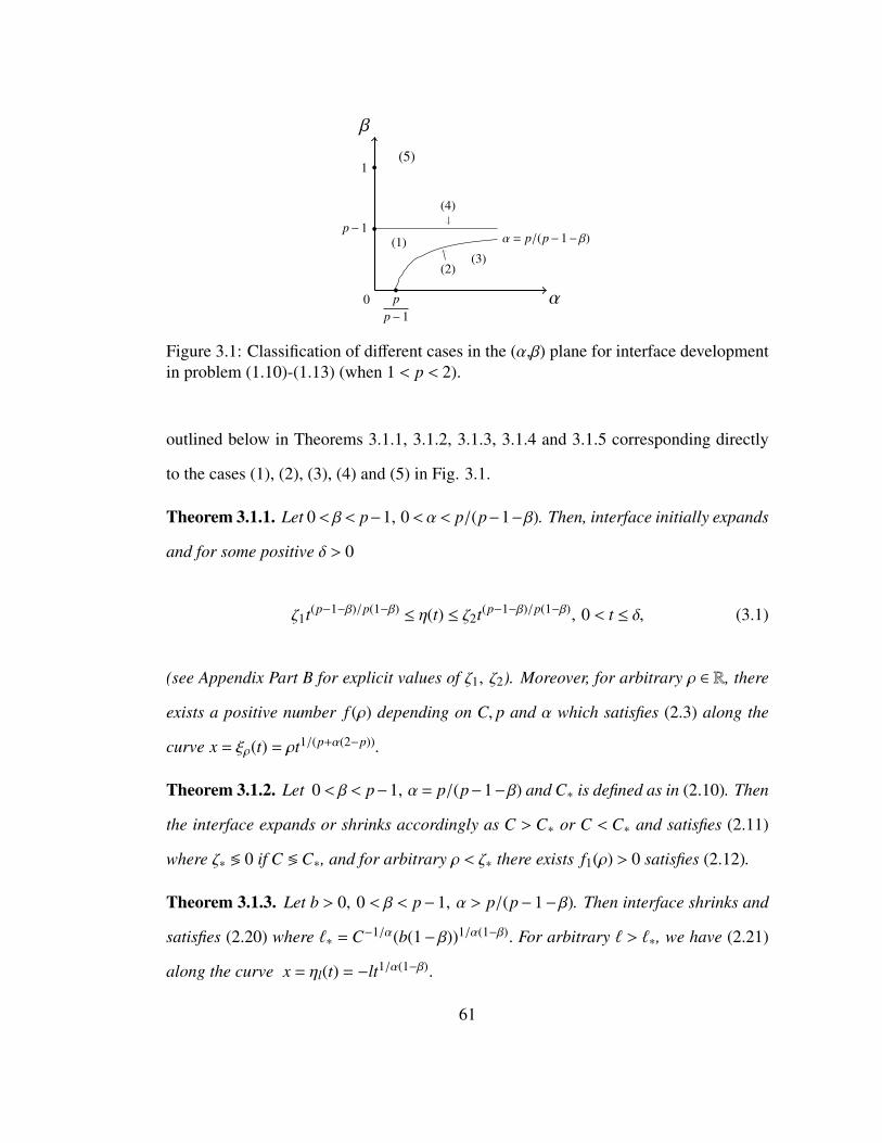
Figure 3.1: Classification of different cases in the (α,β) plane for interface developmentin problem (1.10)-(1.13) (when 1 < p < 2).

outlined below in Theorems 3.1.1, 3.1.2, 3.1.3, 3.1.4 and 3.1.5 corresponding directly

to the cases (1), (2), (3), (4) and (5) in Fig. 3.1.

Theorem 3.1.1. Let 0< β< p−1, 0<α< p/(p−1−β). Then, interface initially expands

and for some positive δ > 0

ζ1t(p−1−β)/p(1−β) ≤ η(t) ≤ ζ2t(p−1−β)/p(1−β), 0 < t ≤ δ, (3.1)

(see Appendix Part B for explicit values of ζ1, ζ2). Moreover, for arbitrary ρ ∈ R, there

exists a positive number f (ρ) depending on C, p and α which satisfies (2.3) along the

curve x = ξρ(t) = ρt1/(p+α(2−p)).

Theorem 3.1.2. Let 0 < β < p−1, α = p/(p−1−β) and C∗ is defined as in (2.10). Then

the interface expands or shrinks accordingly as C > C∗ or C < C∗ and satisfies (2.11)

where ζ∗ ≶ 0 if C ≶C∗, and for arbitrary ρ < ζ∗ there exists f1(ρ) > 0 satisfies (2.12).

Theorem 3.1.3. Let b > 0, 0 < β < p−1, α > p/(p−1−β). Then interface shrinks and

satisfies (2.20) where ℓ∗ = C−1/α(b(1− β))1/α(1−β). For arbitrary ℓ > ℓ∗, we have (2.21)

along the curve x = ηl(t) = −lt1/α(1−β).

61

Theorem 3.1.4. Let b > 0, 0 < β = p− 1 < 1, α > 0. Then there is an infinite speed of

propagation and ∀ ϵ > 0, ∃ δ = δ(ϵ) > 0 such that

t1/(2−p)φ(x) ≤ u(x, t) ≤ (t+ ϵ)1/(2−p)φ(x) for 0 < x <∞, 0 ≤ t ≤ δϵ , (3.2)

where φ(x) solves ODE problem

(|φ′(x)|p−2φ′(x))′ =1

2− pφ(x)+bφp−1(x) (3.3a)

φ(0) = 1, φ(∞) = 0. (3.3b)

Solution u satisfies asymptotic formula

logu(x, t) ∼ −( b

p−1)1/px as x→ +∞. (3.4)

Theorem 3.1.5. Let either b > 0, β > p−1 or b < 0, β ≥ 1 and

D =(2(p−1)pp−1(2− p)1−p

)1/(2−p). (3.5)

Then there is an infinite speed of propagation and (2.3) is valid. If either b > 0, β ≥ 2/p

or b < 0, β ≥ 1 then ∃δ > 0 such that for ∀ fixed t ∈ (0, δ]

u(x, t) ∼ Dt1/(2−p)xp/(p−2) as x→ +∞. (3.6)

62

If b > 0,1 ≤ β < 2/p, then

limt→0+

limx→+∞

ut1/(p−2)xp

2−p = D. (3.7)

If b > 0, p−1 < β < 1 then ∃δ > 0 such that for arbitrary fixed t ∈ (0, δ]

u(x, t) ∼C∗xp/(p−1−β) as x→ +∞. (3.8)

3.2 Further Details of the Main Results

In this section we outline some essential details of the main results described in Theo-

rems 3.1.1 - 3.1.5.

Further details of Theorem 3.1.1. Solution u satisfies the estimation

C1t1/(1−β)(ζ1− ζ)p/(p−1−β)+ ≤ u ≤C∗t1/(1−β)(ζ2− ζ)

p/(p−1−β)+ , 0 < t ≤ δ, (3.9)

where ζ = xt−(p−1−β)/p(1−β) and the left-hand side of (3.9) is valid for 0 ≤ x < +∞, while

the right-hand side is valid for x ≥ ℓ0t(p−1−β)/p(1−β) and the constants C∗, C1, ζ1, ζ2 and

ℓ0 are positive and depend only on p, β and b (see Appendix Part B).

A function f is a shape function of the self-similar solution of (1.10),(1.13) with

b = 0 (see Lemma 3.3.1) and satisfies (2.6) where w is a solution of (1.10), (1.13)

with b = 0, C = 1. Lower and upper estimations for f are given in (2.4), (3.23). If u0 is

defined as in (1.13), then the right-hand sides of (3.9), (3.1) are valid for 0< t <+∞. The

explicit formula (2.3) means that the local behavior of solution along the curves x= ξρ(t)

approaching the origin coincides with that of the problem (1.10), (1.13) with b = 0.

In other words, diffusion completely dominates in this region. However, domination

63

of diffusion over the reaction fails along the curves x = ζρ(t) = ρt(p−1−β)/p(1−β), ρ > 0

approaching the origin and the balance between diffusion and reaction in this region

governs the interface, as expressed in estimations (3.9), (3.1). We stress the fact that the

constants C1, ζ1, ζ2 and ℓ0 in (3.9), (3.1) do not depend on C and α.

Further details of Theorem 3.1.2. Assume that u0 is defined by (1.13). If C = C∗

then u0 is a stationary solution to (1.10),(1.13). If C , C∗ the solution to (1.10),(1.13)

is of self-similar form as in (2.14) and (2.15). If C > C∗ then the interface expands,

f1(0) = A1 > 0 (see Lemma 3.3.3) and

C′(ζ′t(p−1−β)/p(1−β)− x)p/(p−1−β)+ ≤ u(x, t) ≤C′′(ζ′′t(p−1−β)/p(1−β)− x)p/(p−1−β)

+ , (3.10a)

ζ′ ≤ ζ∗ ≤ ζ′′, (3.10b)

where 0 ≤ x < +∞, 0 < t < +∞ and C′ = C2, C′′ = C∗, ζ′ = ζ3, ζ′′ = ζ4 (see Appendix

Part B).

If 0 < C < C∗ then the interface shrinks. There exists a constant ℓ1 > 0 such that for

arbitrary ℓ ≤ −ℓ1, there exists a λ > 0 such that

u(ℓtp−1−βp(1−β) , t) = λt1/(1−β), t ≥ 0. (3.11)

Moreover, u and ζ∗ satisfy (3.10) with C′ =C∗, C′′ =C3, ζ′ = −ζ5 = −ℓ1+ (λ/C∗)

p−1−βp <

0, ζ′′ = −ζ6 and the left-hand side of (3.10a) is valid for x ≥ −ℓ1t(p−1−β)/p(1−β), while the

right-hand side is valid for x ≥ −ℓ2t(p−1−β)/p(1−β) (see Appendix Part B, Lemma 3.3.3

and (3.24)).

In general the precise value ζ∗ can be found only by solving the similarity ODE

64

L0 f1 = 0 (see (2.77b) ) and by calculating ζ∗ = supζ : f1(ζ) > 0.

The right-hand side of (2.11) (respectively (2.12)) relates to the self-similar solution

(2.14), for which we have lower and upper bounds via (3.10). If u0 satisfies (1.12) with

α = p/(p− 1− β),C = C∗ then the small-time behavior of the interface and the local

solution depends on the terms smaller than C∗(−x)p/(p−1−β) in the expansion of u0 as

x→ 0−.

It should be noted that if C > C∗ then the estimation (3.10) coincides with the esti-

mation (2.19), proved for the case β(p−1) < 1, p > 2. If 0 <C <C∗ then the right-hand

side of estimation (3.10) coincides with (2.19) proved for the case β(p− 1) < 1, p > 2,

while the left-hand side of (3.10) is new. It should also be noted that the left-hand side

of the estimation (2.19) proved above for the case β(p− 1) < 1, p > 2, is still valid if

p ≥ 2−β.

Further details of Theorem 3.1.3. The interface initially coincides with that of the

solution (2.22) to the problem (2.23)

Further details of Theorem 3.1.4. The solution of (3.3) is

φ(x) = F−1(x), 0 ≤ x < +∞, (3.12)

where F−1(x) is an inverse function of

F(z) =∫ 1

z

dy

y[ b

p−1 +p

2(p−1)(2−p)y2−p]1/p , 0 < z ≤ 1. (3.13)

φ satisfies

logφ(x) ∼ −( b

p−1

)1/px as x→ +∞. (3.14)

65

and the global estimation

0 < φ(x) ≤ e−(

bp−1

)1/px, 0 ≤ x < +∞. (3.15)

Therefore, for any γ >( b

p−1)1/p we have

limx→+∞

φ(x)e−γx = +∞. (3.16)

Respectively, the solution u satisfies

limt→0+

limx→+∞

u(x, t)e(

bp−1

)1/px= 0, (3.17)

and for any γ >( b

p−1)1/p

limx→+∞

u(x, t)e−γx = +∞, 0 < t ≤ δ. (3.18)

Further details of Theorem 3.1.5. Let β ≥ 1. Then for arbitrary sufficiently small

ϵ > 0 there exists a δ = δ(ϵ) > 0 such that

C5tα/(p+α(2−p))(ξ1+ ξ)p

p−2 ≤ u ≤C6tα/(p+α(2−p))(ξ2+ ξ)p

p−2 x ≥ 0, 0 ≤ t ≤ δ, (3.19)

where ξ = xt−1/(p+α(2−p)) (see Appendix Part B for the relevant constants). If b> 0, β≥ 1,

then the following upper estimation is also valid

u(x, t) ≤ Dt1/(2−p)xp/(p−2) 0 < x < +∞, 0 < t < +∞, (3.20)

Let b < 0, β ≥ 1. Then for arbitrary sufficiently small ϵ > 0 there exists δ = δ(ϵ) > 0

66

such that

u(x, t) ≤ D(1− ϵ)1/(2−p)t1/(2−p)xp/(p−2) for µt1/(p+α(2−p)) < x < +∞, 0 < t ≤ δ,

(3.21)

with

µ =(D−1(A0+ ϵ)

)(p−2)/p(1− ϵ)−1/p.

From (3.19) and (3.21), (3.6) again follows.

Let b > 0, p−1 < β < 1. Then there exists a number δ > 0 such that

C∗(1− ϵ)t1(1−β)(ζ8+ ζ)p/(p−1−β)+ ≤ u(x, t) ≤C∗xp/(p−1−β) 0 < x < +∞, 0 < t ≤ δ.

(3.22)

where ϵ > 0 is an arbitrary sufficiently small number

As in the case I(1), the explicit formulae (2.3) expresses the domination of diffusion

over the reaction. If β ≥ 1, then from (3.19), (3.6), (3.7) it follows that domination of

diffusion is the case for x≫ 1 as well, and the asymptotic behavior as x→ +∞ coincides

with that of the solution to problem (1.10), (1.13) with b = 0 (see the case II below).

However, if p− 1 < β < 1 then domination of the diffusion fails for x≫ 1 and there is

solution of Eq. (1.10) on the right-hand side of (3.8).

(II) b = 0, 1 < p < 2, α > 0.

In the case there is an infinite speed of propagation. First, assume that u0 is defined

by (1.13). Then the solution to (1.10), (1.13) has the self-similar form (2.4) where f

satisfies (2.6). Moreover, we have

Dtα/(p+α(2−p))(ξ3+ξ)p/(p−2) ≤ u ≤C7tα/(p+α(2−p))(ξ4+ξ)p/(p−2), 0 ≤ x, t < +∞ (3.23)

67

(see Appendix Part B). The right-hand side of (3.23) is not in fact sharp enough as

x→ +∞ and the required upper estimation is provided by an explicit solution to (1.10),

as in (3.20). From (3.23) and (3.20) it follows that, for arbitrary fixed 0 < t < +∞, the

asymptotic result (3.6) is valid.

Now assume that u0 satisfies (1.12) with α > 0. Then (2.3) is valid and for arbitrary

sufficiently small ϵ > 0 there exists a δ = δ(ϵ) > 0 such that the estimation (3.23) is valid

for 0 < t ≤ δ, except that in the left- hand side (respectively in the right-hand side ) of

(3.23) the constant A0 should be replaced by A0−ϵ (respectively A0+ϵ). Moreover, there

exists a number δ > 0 (which does not depend on ϵ) such that, for arbitrary t ∈ (0, δ], the

asymptotic result (3.6) is valid.

3.3 Asymptotic Properties of solutions based on scaling

laws

In the next two lemmas, we establish some preliminary estimations of the solution to

CP, the proof of these estimations begin based on scale of variables.

Lemma 3.3.1. If b = 0 and 1 < p < 2, α > 0, then the solution u of the CP (1.10), (1.13)

has the self-similar form (2.4), where the self-similarity function f satisfies (2.6). If u0

satisfies (1.12) then the solution to the CP (1.10), (1.11) satisfies (2.3).

The proof of the lemma coincides with the proof of Lemma 2.3.1.

Lemma 3.3.2. Let u be a solution of the (1.10), (1.11) and let u0 satisfy (1.12). Let one

of the following conditions be valid:

(a) b > 0, 0 < β < p−1 < 1, 0 < α < pp−1−β ;

(b) b > 0, 0 < p−1 < 1, β ≥ p−1, α > 0;

68

(c) b < 0, β ≥ 1, 0 < p−1 < 1, α > 0.

Then u satisfies (2.3) with the same function f as in Lemma 3.3.1.

Lemma 3.3.3. Let u be a solution to the CP (1.10), (1.13) with b > 0, 0 < β < 1, p−1 >

β, α = p/(p−1−β), C > 0. Then the solution u has the self-similar form (2.14). There is

a constant ℓ1 > 0 such that for arbitrary ℓ ∈ (−∞,−ℓ1] there exists λ > 0 such that (3.11)

is valid. If 0 <C <C∗ then

0 < λ <C∗(−ℓ)p/(p−1−β). (3.24)

If C >C∗ then f1(0) = A1 > 0 where A1 depends on p, β, C and b.

Lemma 3.3.4. Let u be a solution to the CP (1.10), (1.12) with b > 0, 0 < β < 1, p−1 >

β, α = p/(p−1−β), C > 0. Then for arbitrary ℓ ∈ (−∞,−ℓ1] we have

u(ℓt(p−1−β)/(p(1−β)), t) ∼ λt1/(1−β) as t→ 0+, (3.25)

where ℓ1 > 0, λ > 0 are the same as in Lemma 3.3.3 and if 0 <C <C∗ then (3.24) is also

valid. If C >C∗ then u satisfies

u(0, t) ∼ A1t1/(1−β) as t→ 0+, (3.26)

where A1 = f1(0) > 0 (see Lemma 3.3.3).

Lemma 3.3.5. Let u be a solution to the CP (1.10)-(1.12) with b > 0, 0 < β < 1, p−1 >

β, α > p/(p−1−β), C > 0. Then for arbitrary ℓ > ℓ∗ (see (2.20)), the asymptotic formula

(2.21) is valid, with x = ηℓ(t) = −ℓt1/α(1−β).

69

3.3.1 Proof of Lemma 3.3.2: Diffusion dominates over the reaction

Proof of Lemma 3.3.2. The proof for cases (a) and (b) coincides with the proof for

case (a) and (b) with b > 0 in Lemma 2.3.2. The proof for (c) coincides (with some

modifications) with the proof for case (b) with b< 0 in the Lemma 2.3.2; namely, instead

of zero boundary condition on the line x = −xϵ and x = −k1/αxϵ (see (2.59) and (2.60)).

we take

u±ϵ(−xϵ , t) = u(−xϵ , t), 0 ≤ t ≤ δ

u±ϵk (−k1α xϵ , t) = ku(−xϵ ,k(α(p−2)−p)/αt), 0 ≤ t ≤ k

p−α(p−2)α δ,

which are used to imply (2.52). Moreover, if β > 1 then to prove uniform boundedness

of the sequence u±ϵk we choose

g(x, t) = (C+1)(1+ x2)α2 (1− νt)

11−β , x ∈ R, 0 ≤ t ≤ t0 =

ν−1

2,

where ν,h∗ are choosen as in (2.62) and

h(x) = (β−1)αp−1(C+1)p−2(1− νt)p−1−β

1−β (1+ x2)(α−2)(p−1)−2−α

2 x2|x|p−2

×(1+ x2

x2 + (p−2)1+ x2

|x|2+ (α−2)(p−1)

)Then, we have

Lkg ≡ gt −(|gx|

p−2gx)

x+bkα(p−β−1)−p

α gβ = (C+1)(β−1)−1(1+ x2)α2 (1− νt)

β1−βS ,

where

S = ν−h(x)+b(β−1)(C+1)β−1kα(p−β−1)−p

α (1+ x2)α(β−1)

2 .

70

Let R = b(β−1)(C+1)β−1kα(p−β−1)−p

α (1+ x2)α(β−1)

2 . Therefore it follows (2.63), where

R = O(kp−2−p/α

)uniformly for (x, t) ∈ Dk

0ϵ as k→ +∞.

Now if β = 1 we take

g = (C+1)exp(νt)(1+ x2)α2

where

ν = 1+maxx∈R

h†(x).

h†(x) = αp−1(C+1)p−2 exp(νt(p−2))(1+ x2)(α−2)(p−1)−2−α

2 x2|x|p−2

×(1+ x2

x2 + (p−2)1+ x2

|x|2+ (α−2)(p−1)

).

Then, we have

Lkg ≡ gt −(|gx|

p−2gx)

x+bkα(p−2)−pα g = (C+1)(1+ x2)

α2 exp(νt)S ,

where

S = ν−h†(x)+bkα(p−2)−pα .

Let R = bkα(p−2)−pα . Since α(p−2)− p < 0, then R→ 0 as k→ +∞.

R = O(kα(p−2)−pα

)uniformly for (x, t) ∈ Dk

0ϵ as k→ +∞.

Moreover, we have for 0 < ϵ≪ 1 which implies (2.64). Hence, ∃ k0 = k0(α; p) such that

for ∀k ≥ k0 the Comparison Theorem 2.4 of [3] implies (2.65). Let G be an arbitrary

71

fixed compact subset of

P =(x, t) : x ∈ R, 0 < t ≤ t0

.

We take k0 so large that G ⊂ Dk0ϵ for k ≥ k0. From (2.65), it follows that the sequences

u±ϵk ,k ≥ k0, are uniformly bounded in G. As before, from the results of [57, 99] it

follows that the sequence of non-negative and locally bounded solutions u±ϵk is locally

uniformly Holder continuous and weakly pre-compact in W1,ploc (R× (0,T )). It follows for

some subsequence k′ (2.66). Since α(p− 1− β)− p < 0, passing to limit as k′ → +∞,

from (2.34) for u±ϵk′ it follows that v±ϵ is a solution to the CP (1.10), (1.11) with b= 0,T =

t0,u0 = (C± ϵ)(−x)α+. From Lemma 3.3.1, the required estimation (2.3) follows.

3.3.2 Proof of Lemma 3.3.3 & Proof of Lemma 3.3.4 : Diffusion &

Reaction are in balance

Proof of Lemma 3.3.3. The first assertion of the lemma is known when p− 1 ≥ 1 (see

Lemma 2.3.3). The proof is similar if β < p− 1 < 1. If we consider a function uk(x, t)

defined as in (2.67). It may easily be checked that (2.67) satisfies (1.10), (1.13). Since

under the conditions of the lemma there exists a unique global solution to (1.10), (1.13)

we have equation (2.68). If we choose k = t1/(1−β) in (2.68), then (2.68) implies (2.14)

with f1(ζ) = u(ζ,1).

To prove the second assertion of the lemma, Take an arbitrary x1 < 0. Since u is contin-

uous, there exists δ1 > 0 such that

(C/2)(−x1)p/(p−1−β) ≤ u(x1, δ) for δ ∈ [0, δ1] (3.27a)

72

If C ∈ (0,C∗) then we also choose δ1 > 0 such that

u(x1, δ) <C∗(−x1)p/(p−1−β) for δ ∈ [0, δ1] (3.27b)

Choose k = (t/δ)1/(1−β) in (2.68) and then taking

x = −ℓt(p−1−β)/p(1−β), ℓ = ℓ(δ) = x1δ−(p−1−β)/p(1−β), δ ∈ (0, δ1]

we obtain (3.11) with

ℓ1 = −x1δ−(p−1−β)/p(1−β)1 , λ = λ(δ) = δ1/(β−1)u(x1, δ), δ ∈ (0, δ1].

If 0 <C <C∗, then (3.24) follows from (3.27b). Let C >C∗, to prove that f1(0) = A1 > 0

it is enough to prove that there exists a t0 > 0 such that

u(0, t0) > 0. (3.28)

If p ≥ 2, (3.28) is a known result (see Lemma 2.3.3). To prove (3.28) when β < p−1 < 1,

Consider the function

g(x, t) =C1(−x+ t)p/(p−1−β)+

where C1 ∈ (C∗,C). If x < t we have

Lg = bgβS , S = 1−(C1

C∗

)p−1−β+

pb(p−1−β)

C1−β1 (−x+ t)(β(1−p)+1)/(p−1−β).

73

we can choose x1 < 0 and t1 > 0 such that

S ≤ 0 if x1 ≤ x ≤ t, 0 ≤ t ≤ t1.

Since u is continuous, we can also choose t1 > 0 sufficiently small that

g(x1, t) ≤ u(x1, t) for 0 ≤ t ≤ t1.

Moreover

g(x,0) ≤ u0(x) for x ≥ x1

Applying Lemma 2.1 of [3] we have

u(x, t) ≥ g(x, t) for x ≥ x1, 0 ≤ t ≤ t1,

which implies (3.28). The lemma is proved.

Lemma 3.3.4 may be proved by localization of the proof given in Lemma 3.3.3.The

proof of Lemma 3.3.5 coincides with the proof of Lemma 2.3.4.

3.4 Proofs of the main results

In this section, we prove the main results for fast diffusion case.

(I) b , 0 and p < 2.

74

3.4.1 Domination by diffusion: Interface expands

Proof of Theorem 3.1.1. The asymptotic estimations(2.3) and(2.6) follow from Lemma

3.3.2. Take an arbitrary sufficiently small number ϵ > 0; from (2.3) it follows that there

exists a number δ1 = δ1(ϵ) > 0 such that

(A0− ϵ)tα

p−α(p−2) ≤ u(0, t) ≤ (A0+ ϵ)tα

p−α(p−2) , 0 ≤ t ≤ δ1, (3.29)

where A0 = f (0) > 0. Consider a function g(x, t) as given in (2.76), then we obtain(2.77).

For the function f1, we take

f1(ζ) =C0(ζ0− ζ)p/(p−1−β)+ , 0 < ζ < +∞

where C0, ζ0 are some positive constants. From (2.77b), we have (2.78). To prove a

lower estimation, we take C0 =C1, ζ0 = ζ1 (see Appendix Part B). Then we have

L0 f1 ≤ bCβ1(ζ1− ζ)pβ

p−1−β+

1−(C1

C∗

)p−1−β+

C1−β1

b(1−β)ζ

p(1−β)p−1−β

1

= 0. (3.30)

From (2.77), it follows that (2.81). Lemma 2.1 of [3] implies that g is a sub-solution of

equation (1.10) in (x, t) : x > 0, t > 0. Since 1/(1−β) > α/(p−α(p−2)), it follows from

(3.29) that there exists a δ2 > 0, which does not depend on ϵ, such that

g(0, t) ≤ u(0, t) for 0 ≤ t < δ2. (3.31)

we also have (2.80a). Now we can fix a particular value of ϵ = ϵ0 and take δ=min(δ1, δ2).

From (2.81), (3.31), (2.80a) and Lemma 2.1 of [3], the left-hand side of (3.9), (3.1)

follow. To prove an upper estimation, first we use the rough estimation (3.20). The

75

estimation (3.20) is obvious, since by Comparison Theorem 2.4 of [3] u(x, t) may be

upper estimated by the solution of equation (1.10) with b = 0. Using (3.20), we can now

establish a more accurate estimation. For that, consider a function g with C0 =C∗, ζ0 =

ζ2 in Gℓ0,δ, where

Gℓ0,δ = (x, t) : ζℓ0(t) = ℓ0t(p−1−β)/p(1−β) < x < +∞, 0 < t ≤ δ.

From (2.77),(2.78) it follows (2.79). Moreover, from (3.20) we have

u(ζℓ0(t), t) ≤ Dℓp/(p−2)0 t1/(1−β) =C∗(ζ2− ℓ0)p/(p−1−β)

+ t1/(1−β) = g(ζℓ0(t), t) for 0 ≤ t ≤ δ.

(3.32)

By applying the Lemma 2.1 of [3] in Gℓ0,δ, the right hand side of (3.9), (3.1) follow

from (2.79), (3.32) and (2.80a).

If u0 is defined as in (1.13), then the CP (1.10), (1.13) has a global solution and from

a Comparison Theorem 2.4 of [3] it follows that the solution may be globally upper

estimated by the solution to the CP (1.10), (1.13) with b = 0. Hence (3.20), (3.32) and

the right-hand side of (3.9) is valid for 0 < t < +∞.

3.4.2 Borderline case: Diffusion & Reaction are in balance

Proof of Theorem 3.1.2. First, assume that u0 is defined by (1.13). The self-similar

form (2.14) follows from Lemma 3.3.3. The proof of the estimation (3.10a) when C >C∗

and the proof of the right-hand side of (3.10a) when 0 <C <C∗ (and of the correspond-

ing local ones when u0 satisfies (1.12)) fully coincides with the proof given in Theorem

2.1.2 for the case 1 < (p−1) < β−1, p > 2 (see (2.16) and (2.19)). To prove the left-hand

76

side of (3.10a), consider a function g from (2.76) with

f1(ζ) =C∗(−ζ5− ζ)p/(p−1−β)+ , −∞ < ζ < +∞

From (2.77),(2.78) it follows that

Lg ≤ 0 in G−ℓ1,∞ (3.33)

Moreover, we have

u(−ℓ1t(p−1−β)/(p(1−β)), t) = λt1/(1−β) =C∗(ℓ1− ζ5)p/(p−1−β)+ t1/(1−β)

= g(−ℓ1t(p−1−β)/p(1−β), t), 0 ≤ t < +∞, (3.34)

(2.87b) and (2.87c), where x0 > 0 is an arbitrary fixed number. By using (3.33), (3.34),

(2.87b) and (2.87c), we can apply Lemma 2.1 of [3] in

G′−ℓ1,∞

=G−ℓ1,∞∩x < x0.

Since x0 > 0 is an arbitrary number the desired lower estimation from (3.10a) follows .

Suppose that u0 satisfies (1.12) with α = p/(p−1−β), 0 <C <C∗. Then from (3.25)

it follows that for arbitrary sufficiently small ϵ > 0 there exists a number δ = δ(ϵ) > 0

such that

(λ− ϵ)t1/(1−β) ≤ u(−ℓ1t(p−1−β)/(p(1−β)), t) ≤ (λ+ ϵ)t1/(1−β), 0 ≤ t ≤ δ.

77

Using this estimation, the left-hand side of (3.10a) may be established locally in time.

The proof completely coincides with the proof given above for the global estimations,

except that λ should be replaced by λ− ϵ. (2.14) and (3.10a) easily imply (2.15) and

(3.10b).

3.4.3 Domination by absorption: Interface shrinks

Proof of Theorem 3.1.3. The asymptotic estimation (2.21) follows from Lemma 3.3.5.

The proof of the asymptotic estimation (2.20) coincides with the proof given in Theorem

2.1.3. In particular, the estimation (2.92) and (2.93) are true in this case as well.

3.4.4 Infinite speed propagation: Diffusion dominates weakly over

the reaction

Proof of Theorem 3.1.4. The asymptotic estimations (2.3) and (2.6) follow from Lemma

3.3.2. From (2.3), (3.29) follows, where we fix a particular value of ϵ = ϵ0. The function

g(x, t) = t1/(2−p)φ(x) is a solution of (1.10). Since 1/(2− p) > α/(p+α(2− p)), there

exists δ > 0 such that

u(0, t) = A0tα

p+α(2−p) ≥ t1

2−p = φ(0)t1

2−p = g(0, t), 0 ≤ t ≤ δ.

u(x,0) = g(x,0) = 0, 0 ≤ x <∞

Therefore, from Lemma 2.1 of [3], the left-hand side of (3.2) follows. Let us prove the

right-hand side of (3.2). As it was mentioned in Section 3.1, the right-hand side of (3.2)

is valid for 0 < t < +∞ if the initial data u0 from (1.11) vanishes for x ≥ 0. For all ϵ > 0

78

and consider a function

gϵ(x, t) = (t+ ϵ)1/(2−p)φ(x),

gϵ(0, t) = (t+ ϵ)1/(2−p)φ(0) = (t+ ϵ)1/(2−p) ≥ ϵ1/(2−p) ≥

≥(A0+ ϵ

)t

αp+α(2−p) = u(0, t), for 0 ≤ t ≤ δϵ =

[(A0+ ϵ

)−1ϵ1/(2−p)] p+α(2−p)α ,

Due to continuity of gϵ and u, ∃ δ1ϵ > 0 such that gϵ(0, t) ≥ u(0, t). Since gϵ is a solution

of (1.10), from the Lemma 2.1 of [3] it follows that

u(x, t) ≤ gϵ(x, t) = (t+ ϵ)1/(2−p)φ(x), for 0 ≤ x < +∞, 0 ≤ t ≤ δϵ . (3.35)

Integration of (3.3) implies (3.12). Global estimation (3.15) (3.16) (3.17) (3.18). By

rescaling x→ ϵ−1x, ϵ > 0 from (3.12) we have

xϵ=

∫ 1

φ( xϵ )

y−1[ bp−1

+p

2(p−1)(2− p)y2−p]−1/pdy.

Change of variable z = −ϵ logy implies

x = F [Φϵ(x)], (3.36)

where

F (y) =∫ y

0

[ bp−1

+p

2(p−1)(2− p)e

(p−2)ϵ z]−1/pdz,

Φϵ(x) = −ϵ logφ(xϵ

).

From (3.36) it follows that

Φϵ(x) = F −1(x), (3.37)

79

where F −1 is an inverse function of F . Since 1 < p < 2 it easily follows that

limϵ→0F (y) =

( bp−1

)−1/py, limϵ→0F −1(y) =

( bp−1

)1/py, (3.38)

for y ≥ 0 and convergence is uniform in bounded subsets of R+. From (3.37), (3.38) it

follows that

− limϵ→0ϵ logφ

( xϵ

)=( b

p−1

)1/px, 0 < x < +∞. (3.39)

By letting y= x/ϵ from (3.39), (3.14) follows. Global estimation (3.15), and accordingly

also (3.17) (3.18) easily follow from (3.12), (3.13).

3.4.5 Infinite speed propagation: Diffusion dominates strongly over

the reaction

Proof of Theorem 3.1.5. Let either b > 0, β > p− 1 or b < 0, β ≥ 1. The asymptotic

estimations (2.3) and (2.6) follow from Lemma 3.3.2. Take an arbitrary sufficiently

small number ϵ > 0. From (2.3), it follows that there exists a number δ1 = δ1(ϵ) > 0 such

that (3.29) is valid. Let β ≥ 1.

Consider a function

g(x, t) = tα/(p+α(2−p)) f (ξ), ξ = xt−1/(p+α(2−p)). (3.40)

We have

Lg = t(α(p−1)−p)/(p+α(2−p))Lt f (3.41a)

80

Lt f =α

p+α(2− p)f −

1p+α(2− p)

ξ f ′−(| f ′|p−2 f ′

)′+bt(p−α(p−1−β))/(p−α(p−2)) f β.

(3.41b)

As a function f we take

f (ξ) =C0(ξ0+ ξ)−γ0 , 0 ≤ ξ < +∞ (3.42)

where C0, ξ0, γ0 are some positive constants. Taking γ0 = p/(2− p) from (3.41b) we

have

Lt f = (p+α(2− p))−1C0(ξ0+ ξ)p

p−2

×[R(ξ)+bt(p−α(p−1−β))/(p−α(p−2))(p+α(2− p))Cβ−1

0 (ξ0+ ξ)p(1−β)

2−p]

(3.43a)

R(ξ) = [α−2(p−1)pp−1(p+α(2− p))(2− p)−pCp−20 + p(2− p)−1ξ(ξ0+ ξ)−1]. (3.43b)

To prove an upper estimation we take C0 =C6, ξ0 = ξ2 (see Appendix Part B). Then we

have

R(ξ) ≥ α(µb−1)µ−1b (3.44)

From (3.43), (3.44) it follows that

Lt f ≥ 0 for ξ ≥ 0, 0 ≤ t ≤ δ2,

81

where

δ2 = δ1 if b > 0, δ2 =min(δ1, δ3) if b < 0

and

δ3 =[αϵ(A0+ ϵ)1−β(−b(p+α(2− p))(1+ ϵ)

)−1](p+α(2−p))/(p+α(β+1−p))

Hence , from (3.41) we have

Lg ≥ 0 for 0 ≤ x < +∞, 0 < t ≤ δ2. (3.45)

From (3.29) and Lemma 2.1 of [3], the right-hand side of (3.19) follows with δ = δ2. To

prove a lower estimation in this case we take C0 = C5, ξ0 = ξ1. If b > 0 and β < 2/p we

derive from (3.43) that

R(ξ) ≤ α+ p(2− p)−1−2(p−1)pp−1(p+α(2− p))(p−2)−pCp−25

= −(p+α(2− p))((2− p)(1− ϵ)

)−1ϵ (3.46a)

Lt f ≤ 0 for ξ ≥ 0, 0 ≤ t ≤ δ4, (3.46b)

where δ4 =min(δ1, δ5) and

δ5 =[(A0− ϵ)1−β(b(2− p)(1− ϵ)

)−1ϵ](p+α(2−p))/(p+α(β+1−p))

.

82

From (3.46) it follows that

Lg ≤ 0 for 0 ≤ x < +∞, 0 < t ≤ δ4. (3.47)

If either b > 0, β ≥ 2/p or b < 0, β ≥ 1, from (3.43) we have

Lt f = (p+α(2− p))−1C5(ξ1+ ξ)2

p−2

×[R1(ξ)+bt(p−α(p−1−β))/(p−α(p−2))(p+α(2− p))Cβ−1

5 (ξ1+ ξ)(2−pβ)

2−p]

(3.48a)

R1(ξ) = [α−2(p−1)pp−1(p+α(2− p))(2− p)−pCp−25 ](ξ1+ ξ)+ p(2− p)−1ξ

= −p(2− p)−1ξ1, (3.48b)

which again imply (3.46b), where δ4 = δ1 if b < 0, δ4 =min(δ1, δ5) if b > 0 and

δ5 = [p(b(p+α(2− p))(2− p)

)−1(A0− ϵ)1−β](p+α(2−p))/(p+α(β+1−p)).

As before (3.47) follows from (3.48b). From (3.29), and Lemma 2.1 of [3], the left-hand

side of (3.19) follows with δ = δ4. Thus we have proved (3.19) with δ =min(δ2, δ4).

Let b > 0, β ≥ 1. The upper estimation of (3.20) is an easy consequence of Lemma

2.1 of [3], since the right-hand side of it is a solution of (1.10) with b = 0. Let b > 0

and β ≥ 2/p. Now we can fix a particular value of ϵ = ϵ0 and take δ = δ(ϵ0) > 0 in

83

(3.19). Then from the left-hand side of (3.19) and (3.20), the asymptotic result (3.6)

follows. However, if b > 0, 1 ≤ β < 2/p, from (3.19) and (3.20) it follows that for ∀

fixed t ∈ (0, δ(ϵ)]

D(1− ϵ)1/(2−p) ≤ liminfx→+∞

ut1/(p−2)xp

2−p ≤ limsupx→+∞

ut1/(p−2)xp

2−p ≤ D,

which easily implies (3.7) in view of arbitrariness of ϵ.

We now let b < 0, β ≥ 1 and prove (3.21). Consider a function

g(x, t) = D(1− ϵ)1/(p−2)t1/(2−p)xp/(p−2)

in G = (x, t) : µt1/(p+α(2−p)) < x < +∞, 0 < t ≤ δ, where µ is defined as in (3.21). Let

g(x, t) = g(x, t) for (x, t) ∈ G\(0,0) and g(0,0) = 0. We have

Lg = D(2− p)−1(1− ϵ)(1/(p−2)t(p−1)/(2−p)xp/(p−2)G in G

G = ϵ +b(2− p)Dβ−1(1− ϵ)(β−1)/(p−2)t(β+1−p)/(2−p)xp(β−1)/(p−2).

We then derive

G ≥ ϵ +b(2− p)Dβ−1(1− ϵ)(β−1)/(p−2)µp(β−1)/(p−2)t(p+α(β+1−p))/(p+α(2−p)) in G.

Hence,

G ≥ 0 in G, for δ ∈ (0, δ0]

δ0 =[(−b(2− p)

)−1D1−β(1− ϵ)(1−β)/(p−2)µp(1−β)/(p−2)ϵ](p+α(2−p))/(p+α(β+1−p))

,

84

which implies

Lg ≥ 0 in G. (3.49a)

Moreover, we have

g|x=µt1/(p+α(2−p)) = (A0+ ϵ)tα/(p+α(2−p) for 0 ≤ t ≤ δ.

From(3.19), it follows that

u|x=µt1/(p+α(2−p)) ≤C6(ξ2+µ)p

p−2 tα/(p+α(2−p))

≤ (A0+ ϵ)tα/(p+α(2−p) for 0 ≤ t ≤ δ.

Therefore, we have

g ≥ u on G \ G, (3.49b)

From (3.49), and Lemma 2.1 of [3], the desired estimation (3.21) follows. Since ϵ > 0 is

arbitrary, from the left-hand side of (3.19) and (3.21) the asymptotic result (3.6) follows

as before.

Let b > 0, p− 1 < β < 1. The left-hand side of (3.22) may be proved as the left-

hand side of (3.9) was earlier. The only difference is that we take f1(ζ) = C∗(1 −

ϵ)(ζ8+ ζ)p/(p−1−β)+ in (2.76), (2.77). The right-hand side of (3.22) is almost trivial, since

C∗xp/(p−1−β) is a stationary solution of (1.10). The important point in (3.22) is that δ > 0

does not depend on ϵ > 0. This is clear from the analysis involved in the proof of the

similar estimation (3.9). From (3.22), it follows that ∀ fixed t ∈ (0, δ], we have

C∗(1− ϵ) ≤ liminfx→+∞

uxp/(β+1−p) ≤ limsupx→+∞

uxp/(β+1−p) ≤C∗.

85

Since ϵ > 0 is arbitrary, (3.8) easily follows.

II. b = 0

First assume that u0 is defined by (1.13). The self-similar form (2.4) and the formula

(2.6) follow from Lemma 3.3.1. To prove (3.23), consider a function g from (3.40),

which satisfies (3.41) with b = 0. As a function f we take (3.42) with γ0 = p/(2− p).

Then we drive (3.43) with b = 0. To prove an upper estimation we take C0 =C7, ξ0 = ξ4

and from (3.43b) we have

R(ξ) ≥[α−2pp−1(p−1)(p+α(2− p))(2− p)−pCp−2

7]= 0,

which implies (3.45) with δ2 = +∞. As before, from (3.45) and Lemma 2.1 of [3],

the right-hand side of (3.23) follows. The left-hand side of (3.23) may be established

similarly if we take C0 = D, ξ0 = ξ3. To prove the estimation (3.20), consider

gµ(x, t) = D(t+µ)1/(2−p)(x+µ)p/(p−2), µ > 0,

which is a solution of (1.10) for x > 0, t > 0. Since

gµ(0, t) ≥ Dµ(p−1)/(p−2) ≥ u(0, t) for 0 ≤ t ≤ T (µ) = [DA−10 µ

(p−1)/(p−2)](p+α(2−p))/α,

the Lemma 2.1 of [3] implies

u(x, t) ≤ gµ(x, t) for 0 < x < +∞, 0 ≤ t ≤ T (µ).

In the limit as µ→ 0+, we can easily derive (3.20). Finally, from (3.23) and (3.20) it

easily follows that for arbitrary fixed 0 < t < +∞ the asymptotic formula (3.6) is valid. If

86

u0 satisfies (1.12) with α > 0, then (2.3) and (3.29) follow from Lemma 3.3.1. Similarly,

we can then prove that for arbitrary sufficiently small ϵ > 0 there exists a δ = δ(ϵ) > 0

such that (3.23) is valid for 0 ≤ t ≤ δ(ϵ), except that in the left-hand side (respectively

in the right-hand side) of (3.23) the constant A0 is replaced by A0 − ϵ (respectively by

A0 + ϵ ). Then we can fix a particular value of ϵ = ϵ0 and let δ = δ(ϵ0) > 0. Obviously,

from the local analog of (3.23) and (3.20) it follows that, for arbitrary fixed t ∈ (0, δ], the

asymptotic formula (3.6) is valid.

87

Chapter 4

Conclusions

The dissertation presents full classification of the short-time behavior of the interfaces

and local solution near the interfaces or at infinity in the Cauchy problem for the non-

linear parabolic p-Laplacian type reaction-diffusion equation of non-Newtonian elastic

filtration in both slow and fast diffusion regimes:

ut =(|ux|

p−2ux)

x−buβ = 0, x ∈R,0< t < T, p> 1,b,β > 0; u(x,0)∼C(−x)α+, as x→ 0− .

The classification is based on the relative strength of the diffusion and absorption forces.

The following are the main results:

• If p > 2,α < pp−1−min1,β , then slow diffusion dominates over the absorption, and

interface expands with asymptotics

η(t) ∼ ξ∗(C, p,α)t1/(p−α(p−2)) as t→ 0+

• If p ≥ 2,0 < β < 1,α = p/(p−1−β) then diffusion and absorption are in balance,

88

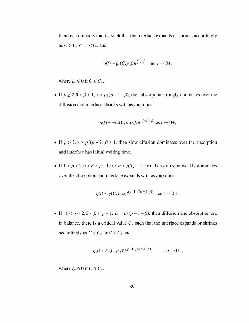
there is a critical value C∗ such that the interface expands or shrinks accordingly

as C >C∗ or C <C∗ and

η(t) ∼ ζ∗(C, p,β)tp−1−βp(1−β) as t→ 0+,

where ζ∗ ≶ 0 if C ≶C∗.

• If p ≥ 2,0 < β < 1,α > p/(p−1−β), then absorption strongly dominates over the

diffusion and interface shrinks with asymptotics

η(t) ∼ −ℓ∗(C, p,α,β)t1/α(1−β) as t→ 0+,

• If p > 2,α ≥ p/(p− 2),β ≥ 1, then slow difusion dominates over the absorption

and interface has initial waiting time.

• If 1 < p < 2,0 < β < p−1,0 < α < p/(p−1−β), then diffusion weakly dominates

over the absorption and interface expands with asymptotics

η(t) ∼ γ(C, p,α)t(p−1−β)/p(1−β) as t→ 0+ .

• If 1 < p < 2,0 < β < p− 1, α = p/(p− 1− β), then diffusion and absorption are

in balance, there is a critical value C∗ such that the interface expands or shrinks

accordingly as C >C∗ or C <C∗ and

η(t) ∼ ζ∗(C, p,β)t(p−1−β)/p(1−β), as t→ 0+,

where ζ∗ ≶ 0 if C ≶C∗.

89

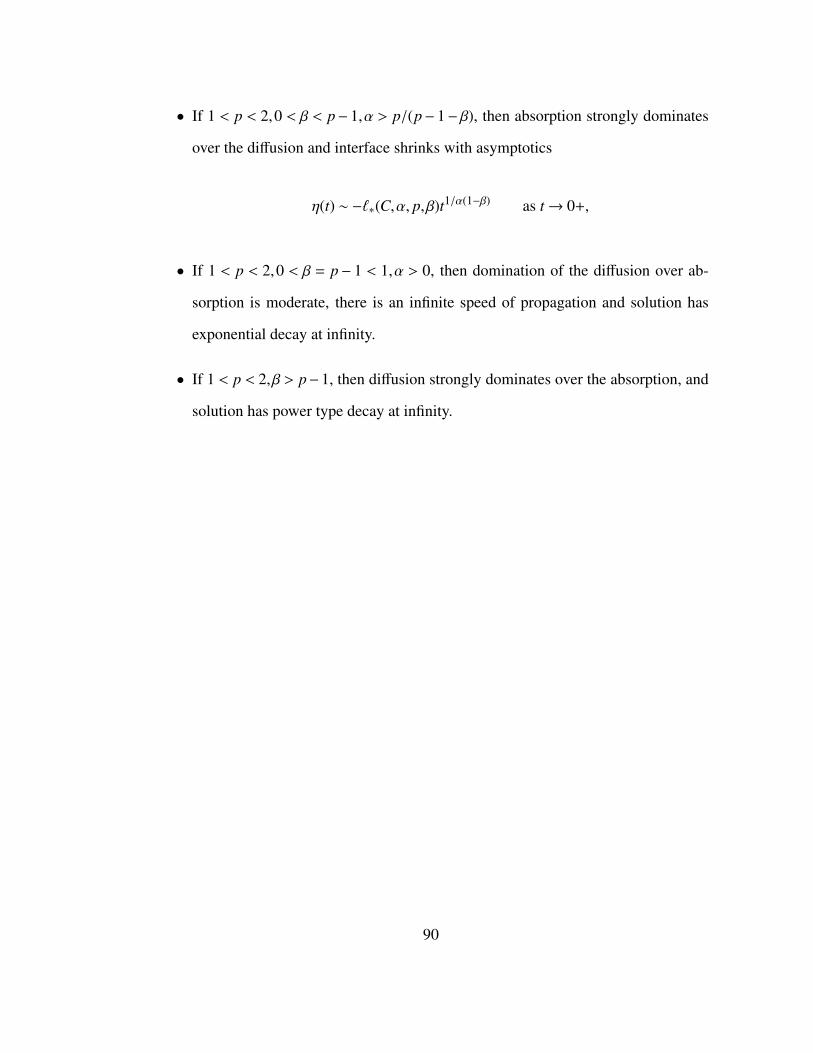
• If 1 < p < 2,0 < β < p− 1,α > p/(p− 1− β), then absorption strongly dominates

over the diffusion and interface shrinks with asymptotics

η(t) ∼ −ℓ∗(C,α, p,β)t1/α(1−β) as t→ 0+,

• If 1 < p < 2,0 < β = p− 1 < 1,α > 0, then domination of the diffusion over ab-

sorption is moderate, there is an infinite speed of propagation and solution has

exponential decay at infinity.

• If 1 < p < 2,β > p−1, then diffusion strongly dominates over the absorption, and

solution has power type decay at infinity.

90

Bibliography

[1] U. G. Abdulla. Local structure of solutions of the Dirichlet problem for N-

dimensional reaction-diffusion equations in bounded domains. Adv. Differential

Equations, 4(2):197–224, 1999.

[2] U. G. Abdulla. On the Dirichlet problem for the nonlinear parabolic equations in

non-smooth domains. In International Conference on Differential Equations, Vol.

1, 2 (Berlin, 1999), pages 729–731. World Sci. Publ., River Edge, NJ, 2000.

[3] U. G. Abdulla. Reaction–diffusion in irregular domains. Journal of Differential

Equations, 164(2):321–354, 2000.

[4] U. G. Abdulla. Reaction-diffusion in a closed domain formed by irregular curves.

J. Math. Anal. Appl., 246(2):480–492, 2000.

[5] U. G. Abdulla. On the Dirichlet problem for reaction-diffusion equations in non-

smooth domains. In Proceedings of the Third World Congress of Nonlinear Ana-

lysts, Part 2 (Catania, 2000), volume 47, pages 765–776, 2001.

[6] U. G. Abdulla. On the dirichlet problem for the nonlinear diffusion equation in non-

smooth domains. Journal of Mathematical Analysis and Applications, 260(2):384–

403, 2001.

91

[7] U. G. Abdulla. Evolution of interfaces and explicit asymptotics at infinity for the

fast diffusion equation with absorption. Nonlinear Analysis: Theory, Methods &

Applications, 50(4):541–560, 2002.

[8] U. G. Abdulla. Nonlinear diffusion in irregular domains. In Elliptic and parabolic

problems (Rolduc/Gaeta, 2001), pages 302–310. World Sci. Publ., River Edge, NJ,

2002.

[9] U. G. Abdulla. First boundary value problem for the diffusion equation. I. Iterated

logarithm test for the boundary regularity and solvability. SIAM J. Math. Anal.,

34(6):1422–1434, 2003.

[10] U. G. Abdulla. Kolmogorov problem for the heat equation and its probabilistic

counterpart. Nonlinear Anal., 63(5-7):712–724, 2005.

[11] U. G. Abdulla. Multidimensional Kolmogorov-Petrovsky test for the boundary

regularity and irregularity of solutions to the heat equation. Bound. Value Probl.,

(2):181–199, 2005.

[12] U. G. Abdulla. Well-posedness of the Dirichlet problem for the non-linear diffu-

sion equation in non-smooth domains. Trans. Amer. Math. Soc., 357(1):247–265,

2005.

[13] U. G. Abdulla. Necessary and sufficient condition for uniqueness of solution to

the first boundary value problem for the diffusion equation in unbounded domains.

Nonlinear Anal., 64(5):1012–1017, 2006.

[14] U. G. Abdulla. Reaction-diffusion in nonsmooth and closed domains. Boundary

Value Problems, 2007(1):031261, 2006.

92

[15] U. G. Abdulla. Wiener’s criterion for the unique solvability of the dirichlet prob-

lem in arbitrary open sets with non-compact boundaries. Nonlinear Analysis: The-

ory, Methods & Applications, 67(2):563–578, 2007.

[16] U. G. Abdulla. Wiener’s criterion at ∞ for the heat equation. Adv. Differential

Equations, 13(5-6):457–488, 2008.

[17] U. G. Abdulla. Wiener’s criterion at ∞ for the heat equation and its measure-

theoretical counterpart. Electron. Res. Announc. Math. Sci., 15:44–51, 2008.

[18] U. G. Abdulla. Regularity of ∞ for the heat equation and the well-posedness of

the Dirichlet problem. In Advances in nonlinear analysis: theory methods and

applications, volume 3 of Math. Probl. Eng. Aerosp. Sci., pages 173–180. Camb.

Sci. Publ., Cambridge, 2009.

[19] U. G Abdulla, J. Du, A. Prinkey, Ch. Ondracek, and S. Parimoo. Evolution of inter-

faces for the nonlinear double degenerate parabolic equation of turbulent filtration

with absorption. Mathematics and Computers in Simulation, 153:59–82, 2018.

[20] U. G. Abdulla and R. Jeli. Evolution of interfaces for the non-linear parabolic p-

Laplacian type reaction-diffusion equations. European J. Appl. Math., 28(5):827–

853, 2017.

[21] U. G. Abdulla and R. Jeli. Evolution of interfaces for the non-linear parabolic

p-Laplacian type diffusion equation of non-Newtonian elastic filtration with strong

absorption. submitted, math arXiv#1811.07278, 2018.

[22] U. G. Abdulla and J. R. King. Interface development and local solutions to

reaction-diffusion equations. SIAM Journal on Mathematical Analysis, 32(2):235–

260, 2000.

93

[23] U. G. Abdullaev. Unbounded solutions of a nonlinear heat equation with a sink.

Zh. Vychisl. Mat. i Mat. Fiz., 32(8):1244–1257, 1992.

[24] U. G. Abdullaev. Existence of unbounded solutions of a nonlinear heat equation

with a sink. Zh. Vychisl. Mat. i Mat. Fiz., 33(2):232–245, 1993.

[25] U. G. Abdullaev. On the localization of unbounded solutions of the nonlinear heat

equation with transfer. Dokl. Akad. Nauk, 329(5):535–537, 1993.

[26] U. G. Abdullaev. Large-time behaviour of solutions of the nonlinear infiltration

equation. Nonlinear Anal., 23(10):1353–1364, 1994.

[27] U. G. Abdullaev. The space localization of unbounded boundary perturbations in

nonlinear heat conduction with transfer. Appl. Math. Lett., 7(6):91–95, 1994.

[28] U. G. Abdullaev. On asymptotically sharp local estimates for finite solutions of a

nonlinear parabolic equation with absorption. Sibirsk. Mat. Zh., 36(5):975–991, i,

1995.

[29] U. G. Abdullaev. On sharp local estimates for the support of solutions in problems

for nonlinear parabolic equations. Mat. Sb., 186(8):3–24, 1995.

[30] U. G. Abdullaev. Local structure of solutions of the reaction-diffusion equations. In

Proceedings of the Second World Congress of Nonlinear Analysts, Part 5 (Athens,

1996), volume 30, pages 3153–3163, 1997.

[31] U. G. Abdullaev. Instantaneous shrinking and exact local estimations of solutions

in nonlinear diffusion absorption. Adv. Math. Sci. Appl., 8(1):483–503, 1998.

[32] U. G. Abdullaev. Instantaneous shrinking of the support of a solution of a nonlinear

degenerate parabolic equation. Mat. Zametki, 63(3):323–331, 1998.

94

[33] R. A. Adams. Sobolev spaces. Academic Press [A subsidiary of Harcourt Brace

Jovanovich, Publishers], New York-London, 1975. Pure and Applied Mathematics,

Vol. 65.

[34] L. Alvarez and J. I. Diaz. Sufficient and necessary initial mass conditions for the

existence of a waiting time in nonlinear-convection processes. Journal of mathe-

matical analysis and applications, 155(2):378–392, 1991.

[35] L. Alvarez, J. I. Diaz, and R. Kersner. On the initial growth of the interfaces in

nonlinear diffusion-convection processes. In Nonlinear Diffusion Equations and

Their Equilibrium States I, pages 1–20. Springer, 1988.

[36] S. Angenent. Analyticity of the interface of the porous media equation after the

waiting time. Proceedings of the American Mathematical Society, 102(2):329–336,

1988.

[37] S. N. Antontsev. The localization of solutions to non-linear degenerating elliptic

and parabolic equations. DOKLADY AKADEMII NAUK SSSR, 260(6):1289–1293,

1981.

[38] S. N. Antontsev, J. I. Dıaz, and S. Shmarev. Energy methods for free bound-

ary problems: Applications to nonlinear PDEs and fluid mechanics, volume 48.

Springer Science & Business Media, 2012.

[39] D. G. Aronson. The porous medium equation, in” nomlinear diffusion

problems”.(a. fasano and m. primicerio, eds.) p. 1–46. Lecture Notes in

Mathematics,//Springer-Verlad, Berlin, page 1224, 1986.

95

[40] D. G. Aronson, L. A. Caffarelli, and J. L. Vazquez. Interfaces with a corner point

in one-dimensional porous medium flow. Communications on pure and applied

mathematics, 38(4):375–404, 1985.

[41] D. G. Aronson and J. L. Vazquez. Eventual c-regularity and concavity for flows

in one-dimensional porous media. Archive for Rational Mechanics and Analysis,

99(4):329–348, 1987.

[42] G. I. Barenblatt. On some unsteady motions of a liquid and gas in a porous

medium. Prikl. Mat. Mekh, 16(1):67–78, 1952.

[43] G. I. Barenblatt. Scaling, self-similarity, and intermediate asymptotics, volume 14

of Cambridge Texts in Applied Mathematics. Cambridge University Press, Cam-

bridge, 1996. With a foreword by Ya. B. Zeldovich.

[44] J. Bear. Dynamics of fluids in porous media. Courier Corporation, 2013.

[45] P. Benilan. Evolution equations and accretive operators. Lecture Notes, Univ. of

Kentucky, 1981.

[46] P. Benilan and H. Toure. Sur l’equation generale ut. Comptes rendus des seances

de l’Academie des sciences. Serie 1, Mathematique, 299(18):919–922, 1984.

[47] P. Benilan and J. L. Vazquez. Concavity of solutions of the porous medium equa-

tion. Transactions of the American Mathematical Society, pages 81–93, 1987.

[48] J. Buckmaster. Viscous sheets advancing over dry beds. Journal of Fluid Mechan-

ics, 81(4):735–756, 1977.

96

[49] L. A. Caffarelli and A. Friedman. Regularity of the free boundary for the one-

dimensional flow of gas in a porous medium. American Journal of Mathematics,

101(6):1193–1218, 1979.

[50] S. Chandrasekhar. Stochastic problems in physics and astronomy. Reviews of

modern physics, 15(1):1, 1943.

[51] E. C. Childs. An introduction to the physical basis of soil water phenomena. A Wi-

ley Intercience Publication John Wiley And Sons Ltd,; London; New York; Sydney;

Toronto, 1969.

[52] S. P. Degtyarev and A. F. Tedeev. On the solvability of the cauchy problem with

growing initial data for a class of anisotropic parabolic equations. Journal of Math-

ematical Sciences, 181(1):28–46, 2012.

[53] E Di Benedetto and MA Herrero. Non-negative solutions of the evolution p-

laplacian equation. initial traces and cauchy problem when 1 < p < 2. Archive for

Rational Mechanics and Analysis, 111(3):225–290, 1990.

[54] J. I. Diaz and R. Kersner. On a nonlinear degenerate parabolic equation in infil-

tration or evaporation through a porous medium. Journal of Differential Equations,

69(3):368–403, 1987.

[55] J. I. Dıaz and L. Veron. Compacite du support des solutions dequations quasi

lineaires elliptiques ou paraboliques. CR Acad. Sci. Paris, 297:149–152, 1983.

[56] J I. Dıaz and L. Veron. Local vanishing properties of solutions of elliptic and

parabolic quasilinear equations. Transactions of the American Mathematical Soci-

ety, 290(2):787–814, 1985.

97

[57] E. DiBenedetto. On the local behaviour of solutions of degenerate parabolic

equations with measurable coefficients. Ann. Scuola Norm. Sup. Pisa Cl. Sci. (4),

13(3):487–535, 1986.

[58] E. DiBenedetto. Degenerate parabolic equations. Universitext. Springer-Verlag,

New York, 1993.

[59] E. DiBenedetto and M. A. Herrero. On the cauchy problem and initial traces for a

degenerate parabolic equation. Transactions of the American Mathematical Society,

314(1):187–224, 1989.

[60] J. R. Esteban and J. L. Vazquez. On the equation of turbulent filtration in one-

dimensional porous media. Nonlinear Analysis: Theory, Methods & Applications,

10(11):1303–1325, 1986.

[61] L. C Evans, B. F. Knerr, et al. Instantaneous shrinking of the support of nonneg-

ative solutions to certain nonlinear parabolic equations and variational inequalities.

Illinois Journal of Mathematics, 23(1):153–166, 1979.

[62] G. Francsics. On the porous medium equations with lower order singular nonlinear

terms. Acta Mathematica Hungarica, 45(3-4):425–436, 1985.

[63] A. Friedman. Partial differential equations of parabolic type. 1964. Holt, Reinhart,

and Winston Inc., New York, 1964.

[64] M. Ganesh and M. C. Joshi. Optimality of nonlinear control systems. Nonlinear

Analysis: Theory, Methods & Applications, 16(6):553–566, 1991.

[65] B. H. Gilding. Holder continuity of solutions of parabolic equations. Journal of

the London Mathematical Society, 2(1):103–106, 1976.

98

[66] B. H. Gilding. A nonlinear degenerate parabolic equation. Annali della Scuola

Normale Superiore di Pisa-Classe di Scienze, 4(3):393–432, 1977.

[67] B. H. Gilding. Properties of solutions of an equation in the theory of infiltration.

Archive for Rational Mechanics and Analysis, 65(3):203–225, 1977.

[68] B. H. Gilding. The occurrence of interfaces in nonlinear diffusion-advection pro-

cesses. Archive for rational mechanics and analysis, 100(3):243–263, 1988.

[69] B. H. Gilding. Improved theory for a nonlinear degenerate parabolic equation.

Annali della Scuola Normale Superiore di Pisa-Classe di Scienze, 16(2):165–224,

1989.

[70] B. H. Gilding. Localization of solutions of a nonlinear fokker–planck equation

with dirichlet boundary conditions. Nonlinear Analysis: Theory, Methods & Appli-

cations, 13(10):1215–1240, 1989.

[71] B. H. Gilding and R. Kersner. Instantaneous shrinking in nonlinear diffusion-

convection. Proceedings of the American Mathematical Society, 109(2):385–394,

1990.

[72] B. H. Gilding and L. A. Peletier. On a class of similarity solutions of the porous

media equation. J. Math. Anal. Appl., 55(2):351–364, 1976.

[73] R. E. Grundy. Asymptotic solution of a model non-linear convective diffusion

equation. IMA journal of applied mathematics, 31(2):121–137, 1983.

[74] R. E. Grundy and L. A. Peletier. Short time behaviour of a singular solution to

the heat equation with absorption. Proc. Roy. Soc. Edinburgh Sect. A, 107:271–288,

1987.

99

[75] R. E. Grundy and L. A. Peletier. The initial interface development for a reaction-

diffusion equation with power-law initial data. Quarterly journal of mechanics and

applied mathematics, 43:535–559, 1990.

[76] M. A. Herrero and M. Pierre. The cauchy problem for ut = um when 0 < m < 1.

Transactions of the american mathematical society, 291(1):145–158, 1985.

[77] M. A. Herrero and J. L. Vazquez. On the propagation properties of a nonlinear

degenerate parabolic equation. Communications in Partial Differential Equations,

7(12):1381–1402, 1982.

[78] K. Hollig and H. O. Kreiss. C∞-regularity for the porous medium equation. Math.

Z., 192(2):217–224, 1986.

[79] K. Ishige. On the existence of solutions of the cauchy problem for a doubly nonlin-

ear parabolic equation. SIAM Journal on Mathematical Analysis, 27(5):1235–1260,

1996.

[80] A. S. Kalashnikov. The occurrence of singularities in solutions of the non-steady

seepage equation. USSR Computational Mathematics and Mathematical Physics,

7(2):269–275, 1967.

[81] A. S. Kalashnikov. The nature of the propagation of perturbations in processes

that can be described by quasilinear degenerate parabolic equations. Trudy S. P.,

1:135–144, 1975.

[82] A. S. Kalashnikov. On a nonlinear equation appearing in the theory of non-

stationary filtration. Trudy. Sem. Petrovsk, 5:60–68, 1978.

100

[83] A. S. Kalashnikov. Propagation of perturbations in the first boundary value prob-

lem for a degenerate parabolic equation with a double nonlinearity. Trudy Sem.

Petrovsk., 8, 1982.

[84] A. S. Kalashnikov. On the dependence of properties of solutions of parabolic equa-

tions in unbounded domains on the behavior of the coefficients at infinity. Sbornik:

Mathematics, 53(2):399–410, 1986.

[85] A. S. Kalashnikov. Some problems of the qualitative theory of non-linear degen-

erate second-order parabolic equations. Russian Mathematical Surveys, 42(2):169,

1987.

[86] R. Kershner. Localization conditions for thermal perturbations in a semibounded

moving medium with absorption. Moscow Univ. Math. Bull, 31(4):52–58, 1976.

[87] R. Kersner. Filtration with absorption: necessary and sufficient condition for the

propagation of perturbations to have finite velocity. Journal of Mathematical Anal-

ysis and Applications, 90(2):463–479, 1982.

[88] J. R. King. Development of singularities in some moving boundary problems.

European Journal of Applied Mathematics, 6(5):491–507, 1995.

[89] B. F. Knerr. The porous medium equation in one dimension. Transactions of the

American Mathematical Society, 234(2):381–415, 1977.

[90] O. A. Ladyzhenskaia, V. A. Solonnikov, and N. N. Ural’tseva. Linear and quasi-

linear equations of parabolic type, volume 23. American Mathematical Soc., 1988.

101

[91] Z. LI, W. DU, and C. MU. Travelling-wave solutions and interfaces for non-

newtonian diffusion equations with strong absorption. Journal of Mathematical

Research with Applications, 33(4):451–462, 2013.

[92] F. Nicolosi. Un principio di massimo generalizzato per le sottosoluzioni deboli

delle equazioni paraboliche lineari del secondo ordine. BUMI (4), 11:354–358,

1975.

[93] O. A. Oleinik, A. S. Kalashnikov, and C. Juj-lin. The cauchy problem and bound-

ary problems for equations of the type of non-stationary filtration. Izvestiya Rossi-

iskoi Akademii Nauk. Seriya Matematicheskaya, 22(5):667–704, 1958.

[94] L. A. Peletier. A necessary and sufficient condition for the existence of an inter-

face in flows through porous media. Archive for Rational Mechanics and Analysis,

56(2):183–190, 1974.

[95] L. A. Peletier. On the existence of an interface in nonlinear diffusion processes.

pages 412–416. Lecture notes in Math., Vol. 415, 1974.

[96] M. H. Protter and H. F. Weinberger. Maximum principles in differential equations.

Prentice-Hall, Inc., Englewood Cliffs, N.J., 1967.

[97] S. Shmarev, V. Vdovin, and A. Vlasov. Interfaces in diffusion–absorption pro-

cesses in nonhomogeneous media. Mathematics and Computers in Simulation,

118:360–378, 2015.

[98] K. Tso. On the existence of convex hypersurfaces with prescribed mean curvature.

Annali della Scuola Normale Superiore di Pisa-Classe di Scienze, 16(2):225–243,

1989.

102

[99] M. Tsutsumi. On solutions of some doubly nonlinear degenerate parabolic

equations with absorption. Journal of mathematical analysis and applications,

132(1):187–212, 1988.

[100] C. J. van Duyn and L. A. Peletier. Nonstationary filtration in partially saturated

porous media. Arch. Rational Mech. Anal., 78(2):173–198, 1982.

[101] J. L. Vazquez. Behaviour of the velocity of one-dimensional flows in porous

media. Trans. Amer. Math. Soc., 286(2):787–802, 1984.

[102] J. L. Vazquez. The interfaces of one-dimensional flows in porous media. Trans.

Amer. Math. Soc., 285(2):717–737, 1984.

[103] J. L. Vazquez. Regularity of solutions and interfaces of the porous medium equa-

tion via local estimates. Proc. Roy. Soc. Edinburgh Sect. A, 112(1-2):1–13, 1989.

[104] J. L. Vazquez. The porous medium equation. Oxford Mathematical Monographs.

The Clarendon Press, Oxford University Press, Oxford, 2007. Mathematical theory.

[105] Y. B. Zeldovich and A. S. Kompaneets. On the theory of propagation of heat with

the heat conductivity depending upon the temperature. Collection in honor of the

seventieth birthday of academician AF Ioffe, pages 61–71, 1950.

103

Appendix

Part A: We give here explicit values of the constants used in section 2.1 in the outline

of the results for Case (I(2)) and later in section 2.4 during the proof of these results.

ζ1 = Ap−2

p (1−β)1p (p−1)

(1+b(1−β)Aβ−1

1)− 1

p (p−2)−1,

C1 = A1ζ−µ1 if β(p−1) > 1,

ζ1 = Ap−2

p1((1−β)(1+β)pp−1(p−1)

) 1p(1+b(1−β)Aβ−1

1)− 1

p (p−1−β)−1,

C1 = A1ζ−

pp−1−β

1 , if β(p−1) < 1,

ζ2 = Ap−2

p1((1−β)(1+β)pp−1(p−1)

) 1p(1+b(1−β)Aβ−1

1)− 1

p (p−1−β)−1,

C2 = A1ζ−

pp−1−β

2 , if β(p−1) > 1,

ζ2 =(A1/C∗

) p−1−βp , C2 =C∗, if β(p−1) < 1,

ζ2 = Ap−2

p1

( p(p−1)p(p−2)1−p(1−β)p(p−2)−β(p−1)+1

) 1p , C2 = A1ζ

−(p−1)(p−2)

2 , if β(p−1) > 1,

ζ2 = Ap−2

p (1−β)1p (p−1)

(1+b(1−β)Aβ−1

1)− 1

p (p−2)−1,

C2 = A1ζ−

(p−1)(p−2)

2 , if β(p−1) < 1,

ℓ0 =C1+β−p

p∗ (C∗/C

) (1−β)(p−1−β)1−β(p−1) (b(1−β)θ∗)

p−1−βp(1−β) ,

ζ3 =C1+β−p

p∗

[(C∗/C

) (1−β)(p−1−β)1−β(p−1)

−1](b(1−β)θ∗)

p−1−βp(1−β) ,

θ∗ =[1−(C/C∗

)p−1−β][(C∗/C

) (1−β)(p−1−β)1−β(p−1)

−1]−1,

ℓ1 =C1+β−p

p[b(1−β)(δ∗Γ)−1

((1−δ∗Γ)−

(1−δ∗Γ

)1−p(C/C∗

)p−1−β)] p−1−βp(1−β) ,

ζ4 = δ∗Γℓ1, Γ = 1− (C/C∗)p−1−β

p , C3 =C(1−δ∗Γ

) p1+β−p ,

where δ∗ ∈ (0,1) satisfies

104

g(δ∗) =max[0;1]

g(δ), g(δ) = δ1+β(1−p)

p(1−β)[(1−δΓ)−

(C/C∗

)p−1−β(1−δΓ

)1−p)],

ℓ∗ =C−1α(b(1−β)

)1/(α(1−β))

ζ5 = ( ℓ∗ℓ )α(1−β)(1− ϵ)ℓ, if β(p−1) < 1,

C6 =(1− ( ℓ∗ℓ )α(1−β)(1− ϵ)

)−α[C1−β− ℓ−α(1−β)b(1−β)(1− ϵ))] 1

1−β .

Part B: We given here explicit values of the constants used in Section 2 in the outline

of the results and later in section 4 during the proof of these results.

(1) when 0 < β < p−1, 0 < α < p/(p−1−β)

C∗ =[(b |p−1−β|p)/((1+β)(p−1)pp−1)

]1/(p−1−β), C1 =

((1−β)/(2− p)

)1/(p−1−β)C∗

ζ1 = bp−2

p(1−β)(pp−1(p−1)

)1/p(1+β)1/p(p−1−β) β(p−1)−1

p(1−β)((2− p)/(1−β)

)(2−p)/p(1−β),

ζ2 = b(p−2)/p(1−β)(p−1)1/p p(p−1)/p(1+β)(2−p)/p(1−β)2(p−1−β)/p(1−β)(2− p)β(p−1)−1

p(1−β (1−β)(p−

1−β)−1,

ℓ0 =p−1−β

1−β ζ2,

(2) when b > 0, 0 < β < 1, β < p−1 < β−1, α = p(p−1−β)−1

ζ3 = Ap−2

p1((1−β)(1+β)pp−1(p−1)

) 1p(1+b(1−β)Aβ−1

1)− 1

p (p−1−β)−1,

ζ4 =(A1/C∗

) p−1−βp , C2 = A1ζ

−p

p−1−β3 ,

ζ5 = ℓ1− (λ/C∗)(p−1−β)/p > 0 (see Lemma 3.3 and (2.51))

ℓ2 =C1+β−p

p[b(1−β)(δ∗Γ)−1

((1−δ∗Γ)−

(1−δ∗Γ

)1−p(C/C∗

)p−1−β)] p−1−βp(1−β) ,

ζ6 = δ∗Γℓ2, Γ = 1− (C/C∗)p−1−β

p , C3 =C(1−δ∗Γ

) p1+β−p , where δ∗ ∈ (0,1) satisfies

g(δ∗) =max[0;1]

g(δ), g(δ) = δ1+β(1−p)

p(1−β)[(1−δΓ)−

(C/C∗

)p−1−β(1−δΓ

)1−p)],

(5) when β > p−1

D =[2(p−1)pp−1

(2−p)p−1

]1/(2−p)

ξ1 = (A0− ϵ)(p−2)/p(1− ϵ)1/pD(2−p)/p if b > 0, 1 ≤ β < (4− p)/p,

ξ1 = (A0− ϵ)(p−2)/pD(2−p)/p if either b > 0, β ≥ (4− p)/p or b < 0, β ≥ 1,

105

C5 = (A0− ϵ)ξp/(2−p)1

A0 = f (0) > 0 (see (2.2) and lemma 3.1)

ξ2 = (A0+ ϵ)(p−2)/p[2(p−1)pp−1(p+α(2−p))µbα(2−p)p

]1/pC6 =

[2(p−1)pp−1(p+α(2−p))µbα(2−p)p

]1/(2−p)

µb = 1 if b > 0, µb = 1+ ϵ if b < 0,

ζ8 =[b(1−β)Cβ−1

∗ (1− ϵ)β−1((1− ϵ)p−1−β−1)](p−1−β)/p(1−β)

II b = 0

ξ3 = (A0/D)(p−2)/p, ξ4 = ξ3(1+ p/α(2− p)

)1/pC7 = D

[1+ p/α(2− p)

]1/(2−p)

106