Face Detection and RecognitionReadings: Ch 8: Sec 4.4, Ch 14: Sec 4.4

• Bakic flesh finder using color (HW4)• Fleck, Forsyth, Bregler flesh finder using color/texture and body parts (the naked people paper)• Rowley & Kanade face detector using neural nets to recognize patterns in grayscale• Eigenfaces: the first “appearance-based” recognition

Object Detection• Example: Face Detection

• Example: Skin Detection

(Rowley, Baluja & Kanade, 1998)

(Jones & Rehg, 1999)

3

Fleck and Forsyth’s Flesh Detector

• Convert RGB to HSI• Use the intensity component to compute a texture map texture = med2 ( | I - med1(I) | )• If a pixel falls into either of the following ranges, it’s a potential skin pixel

texture < 5, 110 < hue < 150, 20 < saturation < 60 texture < 5, 130 < hue < 170, 30 < saturation < 130

median filters of radii 4 and 6

* Margaret Fleck, David Forsyth, and Chris Bregler (1996) “Finding Naked People,” 1996 European Conference on Computer Vision , Volume II, pp. 592-602.

Algorithm 1. Skin Filter: The algorithm first locates images containing large areas whose color and texture is appropriate for skin.

2. Grouper: Within these areas, the algorithm finds elongated regions and groups them into possible human limbs and connected groups of limbs, using specialized groupers which incorporate substantial amounts of information about object structure.

3. Images containing sufficiently large skin-colored groups of possible limbs are reported as potentially containing naked people.

This algorithm was tested on a database of 4854 images: 565 images of naked people and 4289 control images from a variety of sources. The skin filter identified 448 test images and 485 control images as containing substantial areas of skin. Of these, the grouper identified 241 test images and 182 control images as containing people-like shapes.

Grouping

Some True Positives

False Negatives True Negative

Results

7

Object Detection: Rowley’s Face Finder

1. convert to gray scale2. normalize for lighting*3. histogram equalization4. apply neural net(s) trained on 16K images

What data is fed tothe classifier?

20 x 20 windows ina pyramid structure * Like first step in Laws algorithm, p. 220

Preprocessing

Image Pyramid Idea

original image (full size)

lower resolution image (1/4 of original)

even lower resolution (1/16 of original)

Training the Neural Network

• Nearly 1051 face examples collected from face databases at CMU, Harvard, and WWW

• Faces of various sizes, positions, orientations, intensities

• Eyes, tip of nose, corners and center of mouth labeled manually and used to normalize each face to the same scale, orientation, and position

Result: set of 20 X 20 face training samples

Positive Face Examples

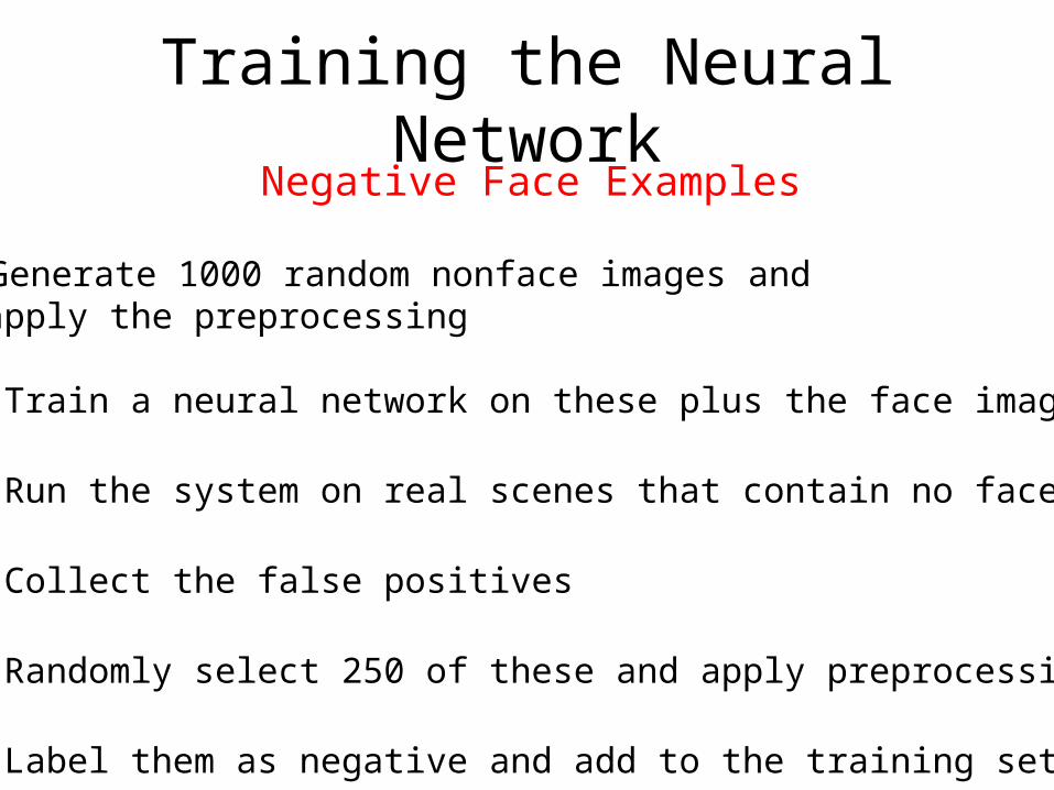
Training the Neural NetworkNegative Face Examples

• Generate 1000 random nonface images and apply the preprocessing

• Train a neural network on these plus the face images

• Run the system on real scenes that contain no faces

• Collect the false positives

• Randomly select 250 of these and apply preprocessing

• Label them as negative and add to the training set

Overall Algorithm

More Pictures

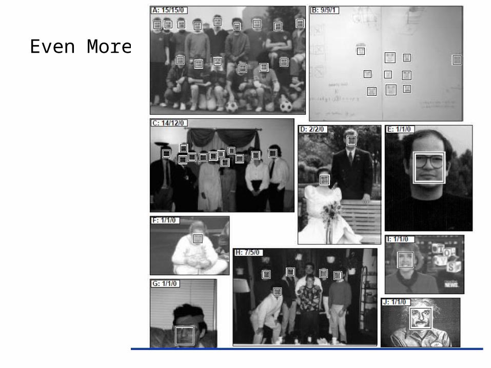
Even More

And More

Accuracy: detected80-90% on differentimage sets with an“acceptable number” offalse positives

Fast Version: 2-4 secondsper image (in 1998)

Object Identification• Whose face is it?

• We will explore one approach, based on statistics of pixel values, called eigenfaces

• Starting point: Treat N x M image as a vector in NM-dimensional space (form vector by collapsing rows from top to bottom into one long vector)

Linear subspaces

• Classification (to what class does x belong) can be expensive– Big search problem

Suppose the data points are arranged as above• Idea—fit a line, classifier measures distance to line

v1 is the major direction of the orangepoints and v2 is perpendicular to v1.

Convert x into v1, v2 coordinates

What does the v2 coordinate measure?

What does the v1 coordinate measure?

- distance to line- use it for classification—near 0 for orange pts

- position along line- use it to specify which orange point it is

Selected slides adapted from Steve Seitz, Linda Shapiro, Raj Rao

Pixel 1

Pixel 2

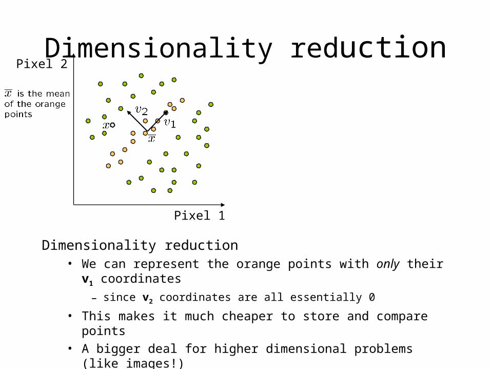
Dimensionality reduction

Dimensionality reduction• We can represent the orange points with only their v1 coordinates

– since v2 coordinates are all essentially 0

• This makes it much cheaper to store and compare points

• A bigger deal for higher dimensional problems (like images!)

Pixel 1

Pixel 2

Eigenvectors and EigenvaluesConsider the variation along a direction v among all of the orange points:

What unit vector v minimizes var?

What unit vector v maximizes var?

Solution: v1 is eigenvector of A with largest eigenvalue v2 is eigenvector of A with smallest eigenvalue

Pixel 1

Pixel 2

A = Covariance matrix of data points (if divided by no. of points)

2

Principal component analysis• Suppose each data point is N-dimensional

– Same procedure applies:

– The eigenvectors of A define a new coordinate system• eigenvector with largest eigenvalue captures the most variation

among training vectors x• eigenvector with smallest eigenvalue has least variation

– We can compress the data by only using the top few eigenvectors• corresponds to choosing a “linear subspace”

– represent points on a line, plane, or “hyper-plane”• these eigenvectors are known as principal component vectors• procedure is known as Principal Component Analysis (PCA)

The space of faces

• An image is a point in a high dimensional space– An N x M image is a point in RNM

– We can define vectors in this space as we did in the 2D case

Dimensionality reduction

• The space of all faces is a “subspace” of the space of all images– Suppose it is K dimensional– We can find the best subspace using PCA– This is like fitting a “hyper-plane” to the set of faces

• spanned by vectors v1, v2, ..., vK

• any face

Turk and Pentland’s Eigenfaces: Training

• Let F1, F2,…, FM be a set of training face images. Let F be their mean and i = Fi – F.

• Use principal components to compute the eigenvectors and eigenvalues of the covariance matrix. M

C = (1/M) ∑iiT

i=1

• Choose the vector u of most significant M eigenvectors to use as the basis.

• Each face is represented as a linear combination of eigenfaces

u = (u1, u2, u3, u4, u5); F27 = a1*u1 + a2*u2 + … + a5*u5

Matching

unknownface image

I

convert to itseigenface representation

= (1, 2, …, m)

Find the face class k that minimizes

k = || - k ||

Eigenfaces• PCA extracts the eigenvectors of covariance matrix A

– Gives a set of vectors v1, v2, v3, ...

– Each one of these vectors is a direction in face space• what do these look like?

Projecting onto the eigenfaces• The eigenfaces v1, ..., vK span the space of faces

– A face is converted to eigenface coordinates using dot products:

Reconstructed face

(Compressed representation of face, K usually much smaller than NM)

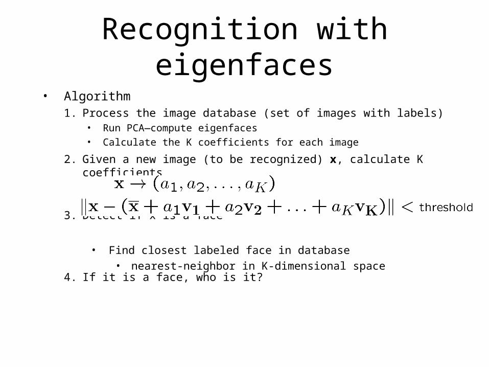
Recognition with eigenfaces

• Algorithm1. Process the image database (set of images with labels)

• Run PCA—compute eigenfaces• Calculate the K coefficients for each image

2. Given a new image (to be recognized) x, calculate K coefficients

3. Detect if x is a face

4. If it is a face, who is it?

• Find closest labeled face in database• nearest-neighbor in K-dimensional space

3 eigen-images

meanimage

trainingimages

linearapproxi-mations

Example

Extension to 3D Objects

• Murase and Nayar (1994, 1995) extended this idea to 3D objects.

• The training set had multiple views of each object, on a dark background.

• The views included multiple (discrete) rotations of the object on a turntable and also multiple (discrete) illuminations.

• The system could be used first to identify the object and then to determine its (approximate) pose and illumination.

Sample ObjectsColumbia Object Recognition Database

Significance of this work

• The extension to 3D objects was an important contribution.

• Instead of using brute force search, the authors observed that

All the views of a single object, when transformed into the eigenvector space became points on a manifold in that space.

• Using this, they developed fast algorithms to find the closest object manifold to an unknown input image.

• Recognition with pose finding took less than a second.

Appearance-Based Recognition• Training images must be representative of the instances of objects to be recognized.

• The object must be well-framed.

• Positions and sizes must be controlled.

• Dimensionality reduction is needed.

• It is not powerful enough to handle general scenes without prior segmentation into relevant objects.

* The newer systems that use “parts” from interest operators are an answer to these restrictions.