Extra, Extra! Read all about it:

The impact of crime reporting by community newspapers

Senior Thesis

Presented to

The Faculty of the School of Arts and Sciences

Brandeis University

Undergraduate Program in Economics

Professor Davide Pettenuzzo, Advisor

In partial fulfillment of the requirements for the degree of Bachelor of Arts

by

Yosef Gabriel Schaffel

May 2013

Copyright by

Yosef Gabriel Schaffel

Committee members (if applicable):

Name: _____________________________ Signature: _____________________________

Name: _____________________________ Signature: _____________________________

Name: _____________________________ Signature: _____________________________

2

Extra, Extra! Read all about it:

The impact of crime reporting by

community newspapers

Yosef Gabriel Schaffel B.A. in Economics and Business, minor in Journalism

Brandeis University, class of 2013

Senior Honors Thesis in Economics

Final Draft – May, 2013

3

I. Introduction

Open up the newspaper. What do you see? If it’s near the front of the issue it’s probably

something you heard on the radio earlier this morning, saw on T.V. last night, or read on the

Internet as soon as the report broke. Most important news is reported far before it is printed in

any daily newspaper, much less a weekly edition. How can print papers report news, often hours

or days after the story has been reported elsewhere, and still remain in business? Yet newspapers

remain a solid, if fading, staple of news distribution.

The Boston Globe is the largest newspaper in Massachusetts and one of the most

recognizable print media outlets in the state. Many other newspapers are also distributed

throughout the region, ranging from huge daily operations such as the Boston Herald to smaller

weekly newspapers. Popular large daily papers tend to cover broad issues, while local papers

focus more on neighborhood stories. There is however an inevitable overlap between local and

state-wide newspapers, such as in crime reporting. Both daily and local papers cover crime news,

especially larger, more attention grabbing crimes. Daily papers and other media outlets often

publish their stories prior to local newspapers, as weekly newspapers are restricted to only

printing news on a set day each week. As a result, local newspapers often repeat crime news

already reported, sometimes up to six days earlier, in daily papers. Further, internet and T.V. are

able to cover crime news before even daily newspapers. The question this project attempts to

address is, if other methods are far quicker and more efficient at reporting on crimes, what is the

impact of crime reporting by small community newspapers?

This question will be addressed through a regression analysis framework. A regression

analysis intends to control numerous factors in order to isolate the effect of one particular aspect

on another. In this study, characteristics of different towns will be held constant while allowing

4

local newspaper circulation to vary, in order to identify only the effects of reporting by local

papers. For example, consider two particular towns that are identical in every way except for

circulation rates. If newspaper reporting has some type of impact on the housing choices of

residents within the towns, one would expect that housing prices would also differ between the

two towns. However, if the house prices are not different between the two towns, this implies

circulation rates of local newspapers have no impact on housing prices.

Specifically, this study will use a regression framework to identify the impact of crime

reporting on an area’s housing prices. For this analysis, an interaction term between crime and

circulation rates will measure any additional effect on real estate prices coming from reading

about crime in a community newspaper. An interaction term is an econometric method of

demonstrating the added benefit of two distinct variables when they are combined.

An example of an interaction term can be seen in oceanfront properties. Owning a house

near the ocean adds value to it. A house with floor-to-ceiling windows also adds value.

However, having a house near the ocean and floor-to-ceiling windows adds another aspect,

distinct from the other two: oceanfront views. This combined effect is captured in a regression

analysis by introducing an interaction term to the regression, which combines these two factors

to track the added effect of both being near the ocean and having floor-to-ceiling windows. The

regression analysis would report distinct impacts for each of the three variables: value added

from being an oceanfront property, value added from large windows, and value added on top of

each of the two if both occur at once.

Following the logic of the above example, crime has been shown in recent works to have

a negative effect on housing prices. (Schwartz et al, 2003), (Linden & Rockoff, 2003), (Ihlanfeldt

& Mayock, 2009) Another main factor is the circulation rate of the papers. A larger readership

5

should result in higher overall awareness and/or a fuller comprehension of issues by a

newspaper’s readership base. Much like combining windows and an ocean view, having more

crime within a particular area and having more readership of a newspaper within that area should

result in a higher overall awareness of crime news, if the crime reporting is having some impact

on its readers. The logic of using this interaction term here has three main assumptions:

1. More crime in an area will result in more crime stories being reported by local

newspapers.

2. Reading about nearby crime in local newspapers will boost perception of crime

in the area, and a higher circulation rate will result in more awareness of crime

stories, further increasing perception.

3. A higher perception of crime will negatively impact neighborhood real estate

prices.

As crime rises within a town, it seems reasonable to assume that a newspaper will report

more crime stories both in raw numbers and as a percentage of all stories. Further, effective

reporting on crime by community newspapers should augment crime perception by potential or

current residents and reduce housing prices. Accordingly, the interaction term of circulation and

crime is, in effect, measuring the increased perception of crime as a result of the newspaper’s

reporting, which is the true factor of interest in my study. This higher awareness should produce

some extra drop in housing prices because perception of crime, as opposed to reported crime,

acting as the true vehicle in which individuals make housing price determinations (Petras, 2003).

If this interaction term of crime and circulation rate is found to be statistically

significant, I can begin to state that community newspapers have at least some degree of

effectiveness in conveying crime news. If not, there is a degree of evidence that community

6

newspapers are partially ineffective in relaying crime information. It is likely that individuals

will learn about neighborhood crime through word of mouth, through a published crime rate, or

other media outlets. If they are finding out about these crimes through other vehicles, why

publish crime stories in a community newspaper at all? If there is no added benefit or no

statistical significance in the interaction term, it begs the question of why this type of reporting is

being performed if individuals are being impacted mainly from other sources.

Finding community newspapers are ineffective in delivering crime news could be a first

step in claiming that community newspapers are an outdated medium. If a population is no better

informed about crime after reading a community newspaper, perhaps it is no better informed

about any issue within the paper. It will be impossible to definitively prove either of these

aspects from just one study, but I hope that this research will serve as springboard for future

projects in which the true value of community newspapers are ascertained.

It must be emphasized again that there are clearly many ways to receive news before

seeing it in a weekly newspaper, such as through internet reporting. In this study, internet

reporting is treated just like large newspapers or like any other competition that community

newspapers face (including the internet iterations of community newspapers themselves). The

amount of media competition facing local newspapers is largely held constant in Massachusetts

towns, either innately or through statistical methods. For example, towns on average have equal

access to internet reports, especially after controlling for median incomes within the towns.

Controlling for these differences between towns is a key part of this analysis. The existence of

internet reporting or other media outlets does not invalidate this study, because it is possible to

track the impact of local newspapers as an isolated entity, distinct from competition, through

regression techniques.

7

In Section II, I will detail the method in which I attempt to ascertain community

newspaper effectiveness in crime reporting. Section III describes the sources of data used, its

qualities, and its limitations. Section IV goes into detail about past literature on crime, housing

prices, and newspaper circulation. Sections V delves into technical questions about the

regression specifications and presents the results and section VI presents a conclusion.

II. Methodology

If community newspapers are effectively transmitting news to their readers, it should be

possible to track how residents react to this news. For example, since crime reduces housing

prices in a neighborhood through less demand to live in the area or more desire to move out,

being more informed about crime should have some further impact on real estate prices. At first

glance, using circulation data within a given town might seem like only residents within the town

are reading about crime news in the local newspaper. Yet, they are not the only potential buyers

of the homes within the town, so it would appear that this data is mostly measuring supply of

homes for sale in the area.

This is not necessarily the case, as it may also measure other factors that impact demand

as well. For example, if a townsperson read a news report and then is asked about crime by an

outside party interested in moving to the town, the community newspaper has potentially

influenced his or her word-of-mouth referral. Because of this, the interaction term described

above may actually capture forces of both demand and supply resulting from a change in

perception due to crime stories in local newspapers. Nonetheless, it should be noted that the most

obvious aspect being measured here is supply side, with peripheral demand-side aspects.

The general regression technique used in this study is an interaction term between the

crime rate and community newspaper circulation in the town, with the dependent variable being

8

housing prices in the area. The logic of using this method has three main assumptions, as

described above:

1. More crime in an area will result in more crime stories being reported by local

newspapers.

2. Reading about nearby crime in local newspapers will boost perception of crime in the

area, and a higher circulation rate will result in more awareness of crime stories,

further increasing perception.

3. A higher perception of crime will negatively impact neighborhood real estate prices.

If these three points hold true, the interaction term measuring the crime and circulation rates

should be a statistically significant and negative, as the extra impact should further decrease real

estate prices. The baseline regression equation is the following:

REPit = β0 +β1CRIit+ β2CIRCit+ β3 (CRIit*CIRCit) +ɣ’Xit+eit

Where REPit= Real estate prices in ith zip code, in year t. CRIit= crime rate in ith zip code, in

year t. CIRCit= circulation density in ith zip code, in year t. Crime data was chosen because it has

been shown to have a clear relationship with real estate prices and it is not difficult to track and

gather crime rates. Circulation numbers are included because they are the best way to quantify a

newspaper’s readership. Finally, as mentioned above, the interaction term is the most important

variable of this study, and is attempting to identify the impact of local reporting on crime.

Crime data is reported as the crime rate, or number of crimes within the population of a

specific zip code. The relationship between crime and real estate prices can also take on other

forms. As the crime rate may be non-linearly related to real estate pricing (Petras, 2003), a non-

linear method was tested, in which a squared variable is introduced. Future works should

9

consider using a crime rate change variable, where crime in the past year is subtracted from the

current year will be tested as well, as per the suggestion of Ihlanfeldt and Mayock in their 2009

paper. They claim that using a change variable instead of a level variable greatly reduces

collinearity between different crime types when using many different crime types. However, my

work uses only two main crime types: property and violent crime. Lagged crime variables should

also be tested, as crime likely does not have an instantaneous effect on housing prices (Ihlanfeldt

and Mayock, 2009), but was not tested here due to time and data constraints.

Finally, a newspaper circulation variable is included in the form of “coverage density,” or

circulation amount per population. This variable, as described above, stands alone in the

regression as well as being included in the interaction term with crime. It is important to note

circulation variables in past research indicated purchase of one newspaper on average was read

by two individuals. (Gentzkow et al., 2006) This finding was carefully considered, as it may

impact crime perception: if two individuals read about a crime event as opposed to one, there

should be some additional effect. However, this previous research was done on larger daily

newspapers and would be too large of an assumption to apply to the drastically different weekly

community papers, so the raw circulation numbers were not manipulated in this study.

Circulation data will be reported on an individual basis as opposed to household basis due to data

constraints.

Another concern is if circulation numbers only track one newspaper per town, while a

town actually has multiple papers, there would be a lower circulation rate that does not

accurately reflect true local newspaper circulation. Local newspaper competition can be

evaluated in a systematic way, as reported household coverage ratios of community newspapers

without competition are far higher than those with similar competition. Further, most towns can

10

only support one local newspaper, as observed from personal research and experience. As a

result, the majority of towns in this study include only one notable community newspaper, so

there is a decreased necessity to consider the impact of direct competitors or market share

dilution. Zip codes with trivial coverage percentages were dropped from the analysis as outliers,

as discussed in the data section.

Endogeneity is a very important concern when considering this methodology.

Specifically, crime is certainly an endogenous variable in the equation. There are countless

observable and unobserved variables that impact crime and also affect real estate prices. For

instance, the median income in a town is usually correlated with both the crime rate as well as

the real estate prices in the area. An unobserved endogenous variable could be a town’s attitude

toward education. If the residents place a very high value on its education system, this could be

correlated with both crime and the overall housing market in the area. With this unobservable

result, other methods must be employed to attempt to avoid problems with internal validity

besides control variables such as median income and education levels. A typical way to control

for unobserved variables is through instrumentation.

Instrumentation, or a two-stage least-squares (2SLS) regression, would be ideal for this

project, as it would allow for elimination of the endogeneity problems mentioned above. A

possible instrument includes the change in police officers in a particular town, along with

controls such as property tax revenue. This should result in a variable that is correlated with

crime, but on a marginal level, may not be correlated with housing prices. Marginal effect

instruments have been notably used by Ihlanfeldt and Mayock (2009). The logic here is a

housing market may not be able to distinguish the added value of one additional police officer in

any way, except through a falling crime rate. Finding an instrument for crime has long been a

11

problem in studies, and will be described in depth in the Literature Review section. Accordingly,

the scope and time limitations of this study ultimately resulted in no instrument being used, as

the change in police officers may prove to not be truly exogenous. Further research is needed to

identify a proper instrument. Other methods will be used in place of instruments, as described

below.

The hedonic method is one such way to reduce problems with endogeneity. A hedonic

method entails decomposing the item being analyzed into particular characteristics, and estimates

the contribution of each individual characteristic towards the whole. Using a hedonic regression

with housing data would mean estimating coefficients for distinct characteristics that comprise

the house. Instead of simply observing average prices of homes in a particular neighborhood, a

hedonic method includes a control variable for bedroom, bathroom, square foot, and so on.

Breaking down the data to such specifics is valuable in controlling for numerous observed

characteristics across houses. It allows for a level of much higher level specificity that may

reduce omitted variable bias. For example, without using a hedonic method, there would be no

distinction between a tiny house in an awful area of town versus a 15 bedroom mansion in a

better area of the same town.

The main benefit in using hedonic regressions is to account for heterogeneity within

homes. It is very difficult to compare buildings based strictly on sales price. By breaking down

the sales price into segmented characteristics of each house, a more specified model is

developed. This can solve for potential endogeneity resulting from correlation of crime with any

specific housing characteristics. For example, if robberies are more likely to occur in larger

homes, including a square feet or bedroom variable in the regression will help reduce this

endogeneity. Though this is just one example, the overarching benefit of using a hedonic model

12

is a higher overall level of specification in the model, resulting in either a better fit, potential

reduction of endogeniety, or both. The issue with the hedonic method is it requires an extremely

rich and detailed dataset that includes all of these specific variables, and this type of data is

difficult to obtain. Fortunately, with access to very rich real estate data, the hedonic method

described above was employed in this study.

The hedonic method is important in crime data as well, as explained by Ihlanfeldt and

Mayock (2009) below. Not using a hedonic method and simply reporting on “crimes” creates no

distinction or weights between differing crime types. As murder has a different impact than auto

theft, this can result in a bias if the two are treated equally. To address this bias, crime will be

segmented from the raw crime rate data, with each crime sorted into being either a violent or a

property crime. While ideally the crimes could be disconnected even further into specific type of

crime, for this study it was unfeasible to do. The reported amounts of particular crimes, such as

arson, larceny, and so on were too small to be considered reliable estimates. It was more reliable

to aggregate these into simply violent or property crimes, as defined by the FBI’s Uniform Crime

Report. Further, it is much more difficult to measure a newspaper’s reporting ability on murder,

versus theft, versus rape, as opposed to a newspaper reporting on violent crimes in general, for

example. Looking at two interaction term variables and deeming the effects of each is simpler

than attempting to explain the interaction between circulation and eight distinct crime types.

Thus it is more sensible to simply aggregate property and violent crimes for the purposes of this

study.

Zip code specific fixed effects will be used to control for unobservable characteristics

across neighborhoods that do not change over time, such as the zip code’s attitude towards

education. Time fixed effects will be included to control for variables that vary over time but are

13

constant across towns in the sample, such as overall changes in the housing market economy.

These fixed effects are critical in reducing omitted variable bias.

There are serious potential issues with this methodology, and most involve omitted

variable bias or endogeneity. As mentioned, there are likely many variables that are correlated

with both crime and the error term not included within the regression. Further, there are also

many variables correlated with the circulation rate and the error. Despite including fixed effects,

some of these variables may vary over both time and place, and may not be captured. This

variation results in omitted variable bias and faulty internal validity, compromising result

findings.

Another common limitation when analyzing crime and real estate interactions is the idea

of simultaneous causality. When looking at the impact of crime on real estate, it is often

impossible to know if rising crime is decreasing real estate prices, or instead if decreasing real

estate prices attract more crime to the area. This is also known as the Granger causality. This

cannot be controlled for in this study and is accepted as a limitation of results.

A last issue to consider is external validity. Due to data limitations, newspaper circulation

data is only available on community newspapers owned by Gatehouse Media. Newspaper

circulation data from entities owned by Gatehouse may act as a proxy for all community

newspapers. However, this study may not be applicable to other locations if it can be shown that

community newspapers owned by Gatehouse Media differ in a systematic way in terms of

location characteristics, reporting style, coverage, or other significant factors. As is shown in the

data section, the distribution of the subsection being used is significantly different than the entire

dataset. This limitation will be discussed further below. Further, this study examines only

14

community newspapers in Massachusetts, specifically those that are without similar competition

in the area. This may limit external validity.

While this methodology is not perfect, and validity problems certainly may exist, issues

with data selection, endogeneity, and assumptions taken are clearly outlined. Problems that

cannot be adequately addressed in any way are recognized in the body of research. However,

potential validity problems occur in any research paper. The goal is to take a realistic view of

data and time available to minimize these problems while still producing a result that the

researcher can stand behind.

III. Data

The main three datasets used in this research are real estate data, crime data, and

circulation data. Other important control variables used are town income and education level

information obtained from the U.S. census.

Real estate data has been obtained from the Multi-Listing Service (MLS) of

Massachusetts web database. This includes individual sales data on the vast majority of home

sold in the state from 2002-2012. Around 10-20% of homes are sold privately, but the remainder

is recorded in MLS. This is roughly 600,000 observations throughout the period. For each

observation, the following data is recorded: List date, sales date, list price, sales price, days on

market, street and number specific address, zip code, area of city, # bedrooms, # bathrooms,

square feet, age of home, size of lot, heating and cooling type, a condo/single family/multifamily

distinction, # fireplaces, among many others. Clearly, this is an extremely comprehensive and

detailed data set which is very important as it allows for the hedonic method previously

described. The range of years allows for a panel data approach. As the data is recorded per

transaction, this allows use of zip code level analysis.

15

This data, unfortunately, was corrupted in places due to human error. All of the

transaction data are entered by hand, so certainly mistakes will be made over the course of

600,000 observations. The hope is that these errors are randomly distributed and have no effect.

Some mistakes, however, were so glaring that it was simple to determine that they were in fact

mistakes and remove them from the data. An entry for a 99 bedroom home is clearly impossible

in all but the rarest of cases, and is likely just code of a missing value. As a result, these obvious

mistakes were detected and dropped from the dataset. The amount of data loss was about 2-3%

of total observations.

Crime data has been gathered from the FBI’s Universal Crime Reports (UCR) for the

state of Massachusetts, on a yearly basis from 2004-2012. The data begins in 2004 because in

2003 and 2002 the UCR uses a different format in which the crime data is less precise. The data

from 2004 and onwards is specified to a city level.

In order to take advantage of zip code level variation in real estate and circulation data,

an assumption has been made to impute crime data across zip codes in the same town. This

assumption follows the logic that by definition, the city crime rate is an average of the crime

rates within the city, so this imputation simply is applying the average crime to each missing zip

code. However, it must be acknowledged that zip code crime levels can vary dramatically, even

within a town. Another option is to aggregate circulation data to the city level, but there would

be a similar issue in which the circulation rate across the entire town would be assumed to be the

aggregate, despite the fact that there is known variation within the zip code. As there are

drawbacks to each method, imputing crime data to the zip code level was deemed the most

efficient and appropriate way to handle the discrepancy in a manner that allowed for maximum

specificity and variation.

16

Another issue with the crime data was missing values across the dataset. This most often

took the form of a town simply being missing from the report for a particular year, likely because

the amount of crime or population was too low to register, but also could be due to bureaucratic

reasons. To address this, the change in crime in surrounding areas was measured, and this

average change was applied to the missing town’s crime value. In this way, all the missing

crime values were imputed. Again, this is an assumption that a particular city’s crime is changing

at the same rate as the towns it is surrounded by, which may or may not always be the case, but

due to restraints was employed here. An alternative was to simply drop towns with missing crime

values, but this would result in a major loss of data of almost 15%, so imputing was judged to be

the more reasonable.

The crime dataset includes total number of property and violent crime, with specific

categories for each, including: murder and manslaughter, rape, robbery, aggravated assault,

burglary, larceny-theft, motor vehicle theft, and arson. It includes population numbers as well,

allowing for a simple conversion to crime rates. The specified types of crimes allow for further

utilization of the hedonic method. The range of years allows for a panel data approach.

Circulation data has been purchased from the Audit Bureau of Circulation (ABC).

However, the circulation numbers required are only the smaller, community newspapers, which

are very difficult to locate, even for the ABC. As a solution to this problem, the ABC has

provided zip code specific circulation numbers of newspapers owned by Gatehouse Media, a

media conglomerate. As mentioned above, this develops a serious concern of sample selection

bias. If Gatehouse Media selects their towns of operation in a systematic way, using only this

subsection of towns certainly could result in sample selection bias. This concern proves to be

true, as can be seen below in Exhibit I. Clearly, the selling prices of houses in the subsection are

17

higher than the entire dataset. Likewise, there is a far higher concentration of lower crime areas

when compared to the complete dataset. These two factors imply that the cities in which

Gatehouse Media is operating do indeed systematically differ.

However, this data may still serve as a suitable proxy for community newspapers, if the

scope of the project is narrowed. By applying the findings to more suburban, upper class areas,

which generally have higher housing prices and lower crime, one is able to compare similar

settings and can justify the data findings, despite the sample selection problem. Further, these

types of areas are most likely to have their own robust community newspapers. Though the areas

of circulation data gathered certainly pose a problem, this data is extremely hard to obtain and as

a result the best way to approach the issue is to reduce the external validity of this project to only

similar communities.

The circulation data ranges from 2004-2012, much like the crime data. The data includes

around 160 distinct zip codes. However, the circulation rates in some zip codes were too low to

be considered realistic and are simply a result of a spillover effect from nearby towns (see

Exhibit II). Towns with circulation rates of less than .01 copies per person were dropped, as it

seems that selling .01 copies per person each week is an unrealistic amount if the newspaper was

truly distributing within the town. For example, the mean population in this study was around

43,500. This circulation figure would mean that only 43 newspapers were sold in the entire

town. It is far more likely that there was spillover of 43 newspapers from a nearby town’s

newspaper as opposed to saying that the town’s own paper sold only 43 copies.

After filtering out these outlying areas, there are around 120 unique zip codes. Using this

subsection of zip code as opposed to the entire MLS real estate database’s zip code set reduces

the sample size to around 140,000 observations. Though this is definitely a large decrease, it

18

should still be a satisfactory sample for a solid analysis as well as statistical relevancy. The

circulation data includes the following variables: zip code, town name, occupied households,

paid newspaper circulation, projected newspaper circulation, and household coverage ratio.

However, the main variables used are simply the zip code and the paid circulation, of which a

circulation rate is then calculated though the crime dataset’s population numbers, to keep a

constant standard of measurement.

Control variables of town income as well as education levels were obtained from the U.S.

Census. Income variables include median income on the zip code level, as well as income

distributions for each zip code. For example, there is a variable for the percentage of town

population earning less than $10,000, making between $10,000 and $15,000, increasing up to

more than $200,000. Education variables include a distribution of education levels within the

town, similar to the income distribution variables. There are variables for the percentage of a

town with less than a high school degree, finished high school, and so on.

Two sets of these variables were obtained, one from the 2000 Census and from the 2011

American Community Survey (5 year). According to the U.S. Census, these two databases are

directly comparable. However, for the purposes of the project, the data is not sufficient, as the

years included are 2004-2011, so the Census data only has information for 2011. To address the

data gap, steps needed to be taken to fill in data for years 2004-2010. By assuming a constant

growth factor from 2000 to 2011, this project attempts to fill in the gaps. For example if income

grew at 10% for a particular zip code from 2000-2011, the growth factor would then be 10%/10

= 1% per year. This growth was applied in reverse to the 2011 variable of that growth category

to fill in data for the missing years. Again, this is a strong assumption that the growth of

particular variables was constant throughout the period, but given the data and time restrictions it

19

was a necessity when using zip code level variables at frequent intervals. This assumption may

prove to be too strong, as seen in the results section. Finally, inflation must be acknowledged.

The income data is in nominal terms for 2000 and 2011. Time fixed effects control for the

majority of inflation, as economy wide inflation likely effects zip codes similarly. Using a simple

linear application of country-wide inflation would not fix anything that time fixed effects do not

capture. However, a way to transform data into real terms should be considered by future

researchers, and is a potential limitation here.

Zip code fixed effects were generated from each zip code in the regression, and time

fixed effects were created for years 2004-2011, with year 2004 being excluded as the baseline.

20

IV. Literature Review

An important aspect in answering the question of effectiveness of community newspapers

is to understand relationship between crime rates and housing prices. Though logic would

suggest that higher crime would lead to less neighborhood desirability and lower housing prices,

this finding has been difficult to conclude in past work. In fact, in 18 recent papers, 14 have

found the expected negative correlation, 3 have been unable to find any statistically significant

effect, and one actually found a positive effect. (Ihlanfeldt and Mayock, 5) This apparent

contradiction can be explained due to the fact that only 6 of the 18 studies [(Rizzo 1979), (Naroff

et al. 1980), (Burnell 1988), (Buck et al. 1993), (Gibbons 2004), (Tita et al. 2006)] treat crime as

endogenous. As there are numerous possible factors that impact both crime and housing prices,

treating crime as exogenous can clearly lead to omitted variable bias. Further, treating crime as

exogenous does not account for simultaneous causality, in which, for example, lower

neighborhood prices attract a higher amount of criminal activity.

This research paper must not only consider the implications of the interaction between

real estate and crime, but it must also inspect the characteristics of real estate pricing on its own,

as well as aspects regarding newspaper, news media and reporting techniques. The following

section will attempt to forward a small number of sources for each subject, to attempt to learn

from their past challenges and successes.

21

i. Housing Prices

David R. Bowes and Keith R. Ihlanfeldt “Identifying the Impacts of Rail Transit

Stations on Residential Property Value” (2001)

Property values have countless inputs and it can be extremely complex to try and price

specific factors that impact the housing price. An example of this is an attempt by Bowes and

Ihlanfeldt to isolate the impact of having a nearby rail station on housing prices. To try and do

so, they use a hedonic model, utilizing single family home sales data in the Atlanta area, as well

as crime data from the FBI and rail station location data from the MARTA (Metropolitan Atlanta

Rapid Transit Authority). As described above, hedonic studies are critical for analysis of

housing prices, as they allows for a more nuanced and intricate analysis, and a hedonic method is

used in my study as well.

The findings of Bowes and Ihlanfeldt imply that different neighborhood characteristics

interact with the same inputs in distinct ways. For example, in a higher crime neighborhood,

being closer to railway station causes a decrease in housing prices. However, in a lower crime

neighborhood, this causes an increase in home value. This finding is troubling, but significant. It

very clearly implies endogeneity, and that the variables which impact housing prices are also

impacted by numerous secondary variables. To explain this through Bowes and Ihlanfeldt’s

study, being between ¼ mile and 3 miles from a rail station in a high income neighborhood

carries a large premium, as it allows higher income residents to have easier commuting access to

their jobs. However, in lower income areas, this premium is apparently outweighed by negative

effects of rail stations, such as pollution, noise, and potential transfer of criminal activity into the

neighborhood. What one can take from their findings is that there are countless unobserved

22

variables that impact housing prices in different ways, and these unobserved variables may even

interact with each other for further impacts on crime.

The implication for my study is that variables cannot simply be observed and linear

housing price conclusions drawn. The control variables such as education level and level of

income are not simple exogenous influences on real estate prices. Rather, the interactions of

observed countless unobserved variables must be accounted for through a variety of methods,

which I attempt to address through neighborhood fixed effects and a hedonic approach, with the

potential for instrumentation.

Karl E. Case and Christopher J. Mayer “Housing Price Dynamics within a

Metropolitan Area” (2001)

When observing changes in real estate prices, it is difficult to isolate the effect of one

particular factor because as mentioned, property pricing is an endogenous subject. Not only can

town specific factors such as median town income influence real estate prices, but statewide

changes also have an impact. For example, a statewide decline in the housing market will

certainly impact most if not all houses throughout the state. Case and Mayer observe particular

wide-reaching variables throughout Massachusetts, such as employment, immigration, school

quality, and housing supply shocks and attempt to define their influences on housing prices.

The Massachusetts home sales data that Case and Mayer use is similar to my own, which

is why their methodology is potentially valuable. Like Case and Mayer, I analyzed a number of

distinct Massachusetts jurisdictions, at the zip code level. One particular aspect of relevance that

Case and Mayer discuss is how the distance to Boston influences both prices and characteristic

makeup of towns.

23

According to Case and Mayer, towns such as Brockton or Leominster, which are

removed from Boston, have concentrations of manufacturing employment, but areas closer to

Boston and downtown Boston itself have more employment based on services and FIRE(finance,

insurance, and real estate.) This is significant because it results in employment of particular

sectors having varying effects on different towns, especially as these levels fluctuate. As workers

tend to live near their jobs, swings in employment in various fields will, as a result, have an

impact on the housing composition of a particular town, as well as its housing supply and

demand. As a result, time fixed effects aiming at controlling for employment rates may not be

successful, as the impact of unemployment can differ radically between different types of towns,

especially those near Boston.

Other findings include that the price premium of a quality public school fell as number of

children who attended public school per family fell, and towns which allowed more construction

had property values rise at a slower rate.

These findings show that such variables as sector-specific employment rates, population

growth, construction rate, and overall shocks to housing supply or demand are clearly correlated

with housing prices. Time fixed effects should control for overall supply or demand shocks to the

entire state, as well as statewide factors such as overall employment level or birth rates because

they likely do not vary to a large degree across towns. Zip code fixed effects will capture such

variation such as the construction rate, as long as this rate is generally constant over time. Most

importantly, however, variables like sector-specific employment may not be captured be either

of these control methods. If one accepts that variation in employment of specific fields affects

towns in differing ways, this may result in variation that changes both over time, and location.

This would render even time and fixed effects useless.

24

The impact for this research is to carefully consider which towns to compare against each

other. Clearly, the makeup of particular characteristics of towns in close proximity to Boston

differ radically from suburban towns, and as the control variables at my disposal may not be

enough to control for differences, a possible approach for my study is to simply exclude those

zip codes near Boston. This largely reduces the issue of comparing drastically different types of

towns, and instead the towns become slightly more uniform. I tested both options of including

these towns as well as excluding them, and figures can be found below in the results section.

ii. Crime and Real Estate Prices

Schwartz et al, “Has Falling Crime Driven New York City’s Real Estate

Prices?”(2003)

As mentioned above, crime has been assumed to have a negative effect on real estate

prices by many researchers, but due to issues that bias results such as treating crime as

exogenous, definitive work has been lacking. Schwartz et al. do not attempt to treat crime as

exogenous, and utilize a hedonic and repeat-sales model, as well as fixed-effects. By doing so,

they are able to begin mitigate the crippling biases of other studies that treat crime as strictly

exogenous.

In the study, Schwartz et al. examine whether a falling crime rate in New York after 1994

was a driving, causal force of the increase in real estate prices. Schwartz et al. obtained crime

data from the New York City Police Department (NYPD) on a precinct level. This data included

breakdowns for specific types of crimes, allowing the researchers to separate effects of violent

and property crime. Having the data at a precinct level is important: The less generalized the

coverage area of crime data is, the further reduced problems of omitted variables becomes.

25

Schwartz et al found a significant impact of crime on real estate prices. Their research

concluded that the drop in violent crime in New York City largely from 1994-1998 accounted for

one-third of the increase in real estate prices in that period. The effect of property crime on real

estate prices was not found to be large.

The main limitations of their findings involve external validity. The research is highly

specific as to reduce omitted variable bias, but the result of this is that the data is not

generalizable. In other words, Schwartz et al. found that in densely populated New York City,

from 1988 to 1998, there was a significant link between violent crime and real estate prices.

However, their work does not apply this finding to less dense cities, or to suburban settings, or to

different periods of time. Their findings are difficult to generalize into an overall statement about

the impact of crime on real estate prices.

Nonetheless, the hedonic and repeat sales methods they utilize go a long way in

controlling for both measured and unmeasured variables, as does using panel data to include

fixed effects in the regression. My study utilizes hedonic and panel data, however repeat-sales

analysis was not feasible. Further studies should attempt to utilize these methods while realizing

that this does not completely solve validity problems.

Linden and Rockoff, “Estimates of the Impact of Crime Risk on Property Values

from Megan’s Laws” (2003)

Linden and Rockoff also grapple with issues of trying to isolate the effect of crime on

real estate. They focus on the impact of convicted sex offenders living in nearby properties.

Having access to the actual location of convicted sex offenders allows Linden and Rockoff to

measure crime much more precisely. As opposed to using a generalized precinct level of crime,

they are able to pinpoint exactly where the “crime” (in this case the previous crime or threat of

26

future crime) is occurring. This accuracy of crime measurement greatly reduces potential

unmeasured variables. For example, instead of generalizing the entire precinct’s attitude towards

crime, Linden and Rockoff can break the segmentation down into block radiuses.

Linden and Rockoff use a hedonic method as well; however, as mentioned above, they

also have extremely detailed geographic locations. By using the introduction of a sex offender to

the neighborhood, Linden and Rockoff are actually able to achieve a quasi-random experiment:

Since in their study the living location of a sex offender is assigned by a mostly random process,

one can observe the specific area within a neighborhood with a sex offender, and compare it to

another area without an offender. This quasi-random experiment removes a multitude of the

problems of validity. It also reduces the problem of simultaneous causality because the sex

offender is an event with a set start date. As opposed to measuring a continuous crime rate, there

is a distinct “before” and “after” period for when a sex offender moves into an area. Because of

this quasi-random experiment, Linden and Rockoff believe they are able to reduce omitted

variable biases significantly, and move closer to establishing a causal relationship.

Linden and Rockoff find that homes within 0.1 miles of the sex offender drop in value by

4%. They find no significant effect for homes further than 0.1 miles. They estimate that a single

sex offender reduces home prices by $4,400, on average.

A main problem with this study is its scope. If one is looking to establish the effect of the

overall crime rate on real estate prices, this study is too specific. The aspect that makes it much

more precise in its measurement also greatly hinders its external validity. It only addresses the

change in real estate prices due to being near a sex offender, rather than per actual crime.

While the study analyzes a sex offense that has already occurred, it simply addresses the

individual preference to not live near a sex offender. Linden and Rockoff claim that the drop in

27

price is because “…estimates suggest that individuals have a strong distaste for living in close

proximity to a sex offender.” (Linden and Rockoff, 1121) However, the “distaste” of living near

a sex offender may not necessarily translate into hesitance of living in a crime ridden area.

Residents certainly may be wary of living near a sex offender, but not necessarily because they

suddenly view the area as having a higher crime rate. Rather, they could see the neighborhood as

“tainted” and prefer to live elsewhere for personal reasons.

Unfortunately, my study does not have access to location based data, rather it is forced to

rely on city crime rates and impute down to a zip code level. Nonetheless, the specificity of

crime data that Linden and Rockoff achieve is certainly the goal of any analysis attempting to

establish a causal relationship between crime and real estate prices.

Tricia L. Petras, “Measuring the Effects of Perceptions of Crime on

Neighborhood Quality and Housing Markets” (2003)

An aspect of determining the relationship between crime and property values is making

the distinction between the reported crime rate and the true crime rate. While the Federal Bureau

of Investigation (FBI) reports a crime rate for each town, this crime rate may not accurately

reflect the true impact on citizens. Residents may disregard certain types of crimes in their

housing market valuation that the FBI chooses to include. Crimes may go unreported that

residents are aware of. Either of these cases would result in the reported crime rate differing from

the “true” crime rate.

Petras addresses the fact that the impact of crime on the housing market is not in fact the

reported crime rate. Rather, housing valuations are mainly dependent on the market’s

“perception” of crime in the area. This perception can be influenced by the reported crime rate,

but the final determination is based on the aggregated individual perception of crime occurring in

28

the market area. As research suggests that the decision to report crime is correlated with the

“socioeconomic characteristics of the neighborhood and the type of crime in question” (Petras

99), the reported crime rate may include unobservable variables that are correlated with

particular neighborhood characteristics, creating a bias. Petras also claims that crime may be

asymmetric in nature, as the pricing reduction from fear of new crime may outweigh gain from

the relief of less crime.

Petras finds no significant differences between using a surveyed crime rate and the

reported crime rate. Petras was also unable to find significant findings to imply that crime is

asymmetric in nature.

Possible reasons for the lack of findings are due to the survey system Petras uses to

measure perception of crime. Questions on the survey were imprecise, and the nature of the

survey was that those answering it were already within the market, while those wishing to buy

homes likely were dependent on word of mouth or published statistics. While a survey system is

a potential way to address perception versus reported crime, the scarcity of quality survey results,

as well as their inherent problems, makes this a daunting task. The reported crime rate remains

the most effective way to measure crime on a large scale, with reservations held as to the

completeness of its reporting. Measured crime statistics may serve as an acceptable proxy for the

perception of crime within a market, with the notable disclaimer that some biases may still exist.

My research uses the published crime rate, while taking these limitations into account.

However, it should again be emphasized that the published crime rate is simply a proxy for the

perception of crime. As crime rises within a town, it is a reasonable assumption that a newspaper

will report more on this crime. As mentioned above, the interaction term of circulation and crime

29

is effectively measuring the increased perception of crime as a result of the newspaper’s

reporting.

Keith Ihlanfeldt and Tom Mayock, “Crime and Housing Prices.” (2009)

As described above, there is serious concern about treating crime as exogenous.

Ihlanfeldt and Mayock go into great detail about previous efforts to describe the relationship

between crime and housing prices. As they write, “Undoubtedly, the endogeneity of crime has

been skirted in the literature for but one reason – it is extremely difficult to identify variables that

satisfy the conditions required of a valid instrument.” (Ihlanfeldt and Mayock, 1) The reasons

they claim that crime cannot be seen as exogenous are threefold. The first is simultaneous

causality, in which an increase or decrease may in real estate prices may actually be causing a

resulting effect in the crime rate. The second reason is potential omitted variable bias, in which

there are factors that affect crime and the housing market that are immeasurable. The final reason

is measurement error, perhaps due to the fact, as stated above, that the reported crime rate does

not equal the actual crime rate.

As Ihlanfeldt and Mayock view crime as endogenous, the majority of their research is

based on finding a suitable instrument to address this problem. The instrument they choose is the

first differenced data for each commercial land use category in each land tract. There are 25

commercial land uses, and as a result, 25 instrumental variables. An expansion or contraction

within these types should be correlated with an expansion or contraction in crime. The logic

behind the instrument is that different types of commercial land will be highly correlated with

specific crime types. As they write, “A new convenience store provides an opportunity to

commit a robbery (a violent crime), while more offices create more locations that can be

burglarized.” (Ihlanfeldt and Mayock, 12) This would show correlation between the instruments

30

and specific types of crime. However, they believe marginal effects of businesses being opened

should not be correlated with housing prices, and this is proved correct in their instrument tests.

Ihlanfeldt and Mayock use panel data of repeat individual home sales with fixed effects.

They also measure the change in crime rate instead of level of crime rate. Doing so results in

lower collinearity, as “crimes by type are far less collinear in changes than in levels.” (Ihlanfeldt

and Mayock, 4)

They find statistically significant data showing that their instruments’ exogeneity could

not be rejected and that a 10% increase in violent crime decreases housing values by 6%. They

find no statistically significant reduction based on an increase in property crime. An explanation

they forward for this is that the mental impact of property crime is far less than violent crime.

Further, the main way to protect against violent crime remains a self-selection towards peaceful

neighborhoods for those who can afford it, as opposed to alarm systems or gates, which can

protect against property crime. This results in heavily reduced demand for violent

neighborhoods, and the corresponding reduction in housing values.

To sum, Ihlanfeldt and Mayock forward very important ideas when analyzing the

relationship between crime and real estate, most importantly the need to use a change variable as

opposed to a levels variable, the need for valid instrumentation, the advantage of panel data,

fixed effects and first-difference equations, as well as the necessity of a hedonic regression. My

work is limited in its scope and resources, but a fuller study will utilize all of these approaches.

Laura Dugan. “The Effect of Criminal Victimization on a Household’s Moving

Decision.” (1999)

The idea of housing neighborhood self-selection that Ihlanfeldt and Mayock forward has

been confirmed in past literature. In her research, Dugan attempts to prove that individuals move

31

out of areas with higher crime. The impact on this towards our research is as mentioned above:

First, if crime occurs, it creates a negative neighborhood characteristic that the population

dislikes. To avoid this characteristic, there is incentive to move. This incentive to move is most

easily accessed by those with higher income, resulting in a transfer of wealth outside of the

crime-ridden neighborhood, and creating an excess supply in the neighborhood. This finally

brings down prices. To sum, if it is accepted that crime causes self-selection out of a

neighborhood, there is a very reasonable explanation and belief as to why the crime rate should

have a negative correlation with real estate prices.

Dugan uses a longitudinal study of crime data from the National Crime Survey, and finds

statistically significant and substantial evidence that following a violent crime in the area or to a

household member, a household is far more likely to move out of the area. For example, after a

nearby crime, Dugan finds that a household is 10% more likely to move. However, she does not

find a distinction between likelihood of moving after property crime versus after violent crime.

While this finding would seem to contradict the explanations of Ihlanfeldt and Mayock in which

only violent crime had a decreasing effect on real estate, there are some issues with Dugan’s

study in this regard. She collected crime data in survey form in which the respondent would

potentially have the ability to report a crime significantly after the crime occurred. As a result of

the vague or possibly inaccurate survey questions, potential measurement error can explain the

seeming contradiction. This leaves room for Dugan’s hypothesis that violent crimes have a

larger impact on an individual’s psyche, and for Ihlanfeldt and Mayock’s conclusion, that violent

crimes have a larger impact on real estate prices. While Dugan’s data was inconclusive in this

regard, it certainly is important to note the significant finding of overall crime being related to

likelihood to relocate, as this justifies a central theory of this paper.

32

iii. Newspapers

Lisa M. George and Joel Waldfogel. “The New York Times and the

Market for Local Newspapers.” (2006)

The particular characteristics of newspapers and print media are important to understand

for my research, as there are significant differences between different types of newspapers, such

as between daily and weekly newspapers, or local versus regional. In their research, George and

Waldfogel attempt to investigate the way in which local newspapers adapted to change when the

New York Times moved into their markets, from 1996-2000. Using data from the Audit Bureau

of Circulations, they transform the zip code based circulation numbers into circulation per capita,

or circulation density. They then examine the impact that the New York Times has after entering

a particular zip code.

George and Waldfogel find that the markets with the highest penetration of New York

Times circulation had a 16 percent lower local newspaper circulation rate among highly educated

readers. However, the local newspaper circulation rate among less educated readers was actually

7 percent higher. George and Waldfogel claim that local newspapers are flexible and are able to

adjust their coverage significantly when faced with competition. As the New York Times is a

publication targeted at the higher educated population segment, George and Waldfogel believe

that local newspapers tweaked their coverage and even writing style to attempt to gain market

share in the lower educated segment.

An important point of George and Waldfogel is the ease with which local newspapers can

adjust their coverage and style. This adaptability of local newspapers has potential implications

for this project. If a local newspaper believes its best competitive interest is to, for example,

cover more graphic crime, and by doing so can influence the public perception of crime, we may

33

encounter a bias. Differing attitude towards reporting on crime can, become an unmeasured

variable, resulting in omitted variable bias.

To address this potential bias in this project, I used panel data with town fixed effects, to

control for unmeasured variables that differ between towns but not over time. This will solve

issues of different editorial and population attitudes towards crime reporting across towns. These

attitudes should not be expected to drastically change over time; there is no reason to believe that

a town population will suddenly clamor for more crime reporting. Even with my dataset using an

umbrella corporation of Gatehouse Media, the individual newspapers are governed town specific

employees in most cases. Accordingly, even in my dataset, the attitude of the editorial staff can

be assumed to remain generally constant over time given the absence of outside interference. My

project begins in 2004, so any coverage adjustments resulting from the entry of the New York

Times should already have taken effect. Because of this, using town fixed effects should solve

most of the issues of varying attitudes towards crime coverage, and as a result, variances in

actual coverage of crime reporting across towns.

Matthew Gentzkow, Jesse M. Shapiro, and Michael Sinkinson. “The Effect of

Newspaper Entry and Exit on Electoral Politics.” (2006)

Newspapers can carry the potential to not only spread news that impacts property values,

but the newspaper itself can even be innately valuable to a city. Gentzkow et al. find in their

research that for each additional daily newspaper in an area, the voting turnout for both

presidential and congressional races was increased by 0.3%. If, as is widely accepted, voting

turnout is viewed as a positive element in society, it would follow that more newspapers would

carry with them positive externalities that may or may not be captured by the real estate market.

34

Gentzkow et al. collected newspaper data for daily newspapers. As our research is more

focused on local town newspapers, which are most often weekly based, their findings cannot

translate exactly. However, the crux of their findings, that having a newspaper in a location may

carry positive externalities, is worth considering for this research.

The complex issue of unmeasured positive or negative externalities associated with

newspapers is difficult to address. However, using panel data with town fixed effects would

hopefully capture the differences in positive and negative externalities from newspapers across

towns, as it is unlikely that these externalities would change drastically over time. Further, the

pure variable of increasing local readership seemed to have a direct, statistically significant

impact on real estate prices, which will be discussed in the results section.

Ying Fan. “Ownership Consolidation and Product Characteristics: A Study of the

U.S. Daily Newspaper Market.” (2006)

Considering how to treat the different types of coverage and the overall amount of

coverage in newspapers is central to my work, as it allows me to better understand the way that

newspapers deliver news. Ying Fan addresses the impact of merges between larger daily

newspapers. Fan creates a model that attempts to measure the impact on utility before and after a

merge. She uses county level circulation data from the Audit Bureau of Circulation and specific

newspaper characteristics. Fan finds, in her particular case study, that a merger would be

responsible for a decrease in welfare of $-3.28 million. She also finds that the change in

characteristics of the newspaper after the merger, such as local news ratio or variety of coverage,

accounts for a welfare loss to readers of $1.05 million.

The aspect of Fan’s work that is important for my methodology is her claim that covering

more local news adds utility to the consumer in some way. In my case, it would be through a

35

more detailed crime report or a report on crime not covered by other avenues. However, it is

important to note past works in which a local reporting element is seen as a positive impact.

36

V. Results

As described, the main variable for this project is the interaction term between crime rate

and circulation rate. However, many other variables must be included as controls to achieve a

valid result. Running a simple OLS regression with strictly both crime types, their nonlinear

components, interaction terms, and controls resulted in curious coefficients. For example, the

regression implies that an increase from the median of 1 violent crime per 1,000 (See Table 1,

regression 1 below) results in an increase in real estate prices in the zip code of 0.5%.1 Though

the value eventually becomes negative at higher crime levels, the fact that the result is implying a

positive correlation of crime and real estate prices at the median level is puzzling. It appears as

though this coefficient is being influenced by other factors. More controls are needed to reduce

omitted variable bias, and these coefficients should not be interpreted as causal.

Hedonic controls, linear income and education controls, as well as fixed effects were

added in regression 2. (See Table 1, regression 2) In this model, the added controls flip the sign

on crime to have the linear term become negative, but the squared term as positive. It should be

noted that only the property crime squared term was statistically significant in a t-test, while the

violent crime squared term was not.2 This regression suggests that violent crime is linear, but

property crime is not. It suggests that every additional violent crime per 1,000 decreases housing

prices in the zip code by 1.94%. It also implies that moving from the median value of property

crime by 1 crime per 1,000 decreases real estate prices by .9%. These results seem reasonable.

Though the violent crime coefficients may be sensible, the main variables of note are the

interaction terms. Thinking logically, the interaction terms should be negative. If newspapers are

1 The nonlinear terms for both violent crime and property crime were jointly significant in F-tests at the 5% level in both this regression and in

every following listed regression. 2 The nonlinear terms for both violent crime and property crime were jointly significant in F-tests at the 5% level in both this regression and in

every following listed regression.

37

spreading awareness of crime, it would not be sensible for this spreading of news to increase the

desire to buy a house or live in the neighborhood. However, in regression 2, this is exactly what

we see. At median levels of crime and circulation, the property crime coefficient implies a

statistically significant increase in housing prices of 2.1% due to crime reporting. Further, this

effect rises as both property crime and circulation rise. If each increases from the median by 1

per 1,000, real estate prices rise a further 0.8%. A similar situation emerges with the violent

crime interaction. At the medians of violent crime and circulation per 1,000, the interaction

effect reports a positive impact on real estate prices of 1.4%. Again, an increase of 1 per 1,000

from the median of both circulation and violent crime results in an increase of real estate prices

of 0.45%. Since it is difficult to accept the interaction terms as significantly positive, more work

was required to refine the regression.

A possible reason for the unforeseen result of the interaction terms in regression 2 is that

income and education are being treated linearly. Reason dictates that as your income rises, the

amount of that income you will be using on a house will not stay the same. For example,

increasing your income by $10,000 when you have $50 million likely will not have the same

effect on your housing preferences compared to if you have $45,000. The following regressions

were attempts to find the proper way to treat the nonlinearity in income.

i. Non-linear Income: Squared and Log forms

Regressions 3 and 4 (See Table 1, regressions 3 and 4) treat income as nonlinear by

squaring it or converting it into a natural log, respectively. 3 An issue is discovered in the results.

The coefficient on the linear median income variable is flipped to a negative by adding its square

3 Median income per 1000 and Median Income per 1000^2 were jointly significant in an F-test at the 5% level.

38

as seen in regression 3. This implies that at lower levels of income, increasing median income

actually reduces real estate prices in a town. For example, the average median income of towns

in this study is almost $70,000.4 The coefficients of median income in regression 3 imply that

moving from a $70,000 to an $80,000 town actually decreases average real estate prices in the

zip code by 1%. This seems to be a counterfactual coefficient. It implies that the higher income

is in a zip code, the less money houses sell for, holding everything else constant. Still, as income

is a control variable, it does not necessarily bias the results of the variables of note, in the

interaction terms. In fact, it is controlling for irregularities in income; that is the point of

including the control. However, more importantly, a significant positive interaction term

remained in regression 3, specifically with violent crime. This is an issue with using regression 3

for reasons outlined above.

The attempt to use log of median income in regression 4 did not fare better. The

coefficient suggests that for every percent that median income increases, housing prices drop by

11%. Further, both interaction terms are positive and statistically significant here as well.

ii. Non-linear Income: An imputation issue?

After extensive work and transformation of variables between logs, squared terms, and

income dummy variable buckets, I believe the regressions issues are not strictly due to incorrect

functional form. Rather, they may be linked to the assumption stated above in the data section

when imputing income levels across the 10 year period. As mentioned, median income data is

only available for 2011 and 2000. To fill in the years in between, a linear growth rate was

assumed. However, this is a very problematic assumption, especially considering the reality of

4 While this may seem high, recall that the data being analyzed is only a subsection of the entire state of Massachusetts; specifically, it is more

suburban and upper class. With that being said, the average median income in a zip code within the entire dataset was $68,755.

39

economic movements. The economy has clearly not been constantly growing, or shrinking, at a

certain percent every year. In fact, it had a large crash right in the middle of this dataset, between

2007 and 2009. One easy outside reference of this is seen very clearly by looking at stock prices.

From October 2007 to March 2009, the S&P 500 decreased by 56.6%. Though a stock index

does not directly mirror changes in income, at the very least the huge drop suggests that

economic changes were not moving in a linear direction within the dataset time period.

Though overall moments in the economy are captured by time fixed effects, the zip code

specific moments are not. If income within a particular zip code changes in a way that is not the

overall effect, these changes will not be absorbed. The effects of the recession or other economy-

wide changes are not constant over zip code, and affect different zip codes in different ways. In

other words, income levels vary over both time and zip code, and as a result are not captured by

either fixed effect. The reason behind including median income variables is to control for these

income deviations over time from the general economy. However, if as mentioned above they

are imputed incorrectly, median income controls may not be controlling the variances

successfully.

A simple example to demonstrate this is by looking at Newton, MA. Median income in

Newton in 2000 was $99,076, and through 2010 rose to $130,313. A linear growth in median

income would show an overall increase of 31.5%, or 3.15% per year. However, this constant

3.15% yearly growth seems unlikely. Particularly, income was likely rising at a higher rate than

this from 2000-2006, and then had a period of much lower growth or even negative growth

during the crash in 2007-2009. Accordingly, median house selling prices in Newton from 2004-

2006 (the earliest the data begins) were $750,000. During the crash in 2007-2009 the median

sales price was $275,000, a staggering drop of $475,000 or 63%. However, due to the

40

imputation method, the regression will register an income level that rose at 3%, but housing

prices that fell 63%. This will appear as a negative impact of income on housing prices. Though

the bulk of economy wide effects may be controlled for by time effects holding constant overall

crash, Newton may have been affected particularly harshly or less severely by the recession. In

fact, it is likely that many towns differed significantly that the effect controlled for by time fixed

effects. In terms of housing prices or median income, this will be an omitted variable, and may

explain the negative income coefficients.

The unreliable imputation of median income is certainly a limitation. Time and data

restraints were too large to replace the data or attempt other solutions to solve it directly. The

issue is clearly demonstrated in Table III, in which a cross-sectional regression was run for only

the year 2011. This year had original, non-imputed data. The results show that median income

has a positive, statistically significant effect. It is only when the income number becomes

imputed across time that income turns negative.

iii. Non-linear Income: Income distribution approach

Numerous attempts were made to work around the income problem. No solutions solved

it directly. Clearly, the best way to address this is to just obtain new income data that does not

have to be imputed. Due to time and data restraints, this was not possible. However, a future goal

of this project is to purchase IRS tax datasets that contain this level of information. This data or

other income measures could improve on the income coefficients.

One method did allow for a more logical finding in the variables of note, in the

interaction terms. Controlling for income distributions within towns resulted in a very sensible

regression output (Table 1, regression 5). The log of income is no longer negative, but is

statistically insignificant. A possible explanation is the imputation was so incorrect that income

41

became difficult to attach to real estate prices and instead was seen as insignificant. The fact that

it is not significant is still troubling, but less so than being negative. More importantly, the

interaction terms of property and violent crime are not significant at the 5% level.5 A finding of

no significance is an improvement over a positive finding due to the issues with a positive

coefficient described above. It should be noted that this is not the only sensible outcome. Any

result where these interactions have a negative outcome on housing prices is certainly acceptable.

However, between having a positive impact on prices and being insignificant, the preferred

specification is they are insignificant.

A final interesting finding is that the circulation rate per 1000 was not statistically

significant. This implies that community newspapers cannot be proven to have an impact on

housing prices based on their circulation rate, as will be discussed below.

The buckets of income distribution included a range from $35,000 to more than

$150,000, with less than $35,000 being omitted. The buckets all sum to 1, so any addition to one

bucket is a subtraction from another, resulting in a zero sum change.

The bucket of those earning between $50,000 and $75,000 is statistically significant and

positive which is sensible when compared to the omitted bucket, which accounts for the

percentage earning less than $35,000. However, a problem remains in that those earning between

$75,000 and $150,000 is significant and is heavily negative. The interpretation on this coefficient

is that for every additional percent earning between $75,000 and $150,000, housing prices

actually drop by 1.57%. This finding, again, seems to be counterfactual. The percentage earning

more than $150,000 was not statistically significant.

5 The interaction terms of (violent crime per 1000 * circulation per 1000) and of (violent crime^2 per 1000 * circulation per 1000) were not jointly

significant in an F-test at the 5% level.

The interaction terms of (property crime per 1000 * circulation per 1000) and of (property crime^2 per 1000 * circulation per 1000) were not

jointly significant in an F-test at the 5% level.

42

One possible explanation is that zero sum coefficients are very hard to interpret. Perhaps

when those earning between $75,000 and $150,000 decreased in percentage, the change was

added to those making more than $150,000. This would potentially result in an increase in

housing prices, as the individuals are making more money, but would show that specifically the

bracket of 75-150 was negatively correlated with housing prices.

The more likely explanation is the negative income imputation problem was not fixed by

adding in buckets, only isolated to the main problem area: Those with towns that have a high

percentage of individuals earning between $75,000 and $150,000.

This specification was used to test for non-linearity in education levels, but results were

very similar. The violent crime coefficient dropped only .001%, from .0134 to .0124. The

interaction terms remain consistent. As a result, the regression used was regression 5. Though

this regression has a troubling coefficient for income distributions between $75,000 and

$150,000, regression 5 produced the most accurate results after taking all factors into account.

iv. Internal Validity

Though this specification has flaws, it was determined to be the best option to use. As a

result, this regression format will be used to convey results. Though income figures seem

compromised, income is being controlled for and may not bias overall findings, but instead

implies issues with income data. Results are, however, impacted by endogeneities that are

present within the regression, such as those that are correlated with crime and real estate prices,

are unobserved, and vary over both time and zip code. Generally, issues with internal validity

here include endogeneity, incorrect functional form, and sample selection bias. These issues can

be solved through a better income variable, instrumenting for crime, and obtaining a richer

circulation dataset to reduce sample selection.

43

v. External Validity

External validity is debatable because this data comes from a subsection of Massachusetts

in two ways. First, it is only covering newspapers and zip codes in which Gatehouse Media

operates. As seen in Exhibit I, the subsection does differ significantly from the entire sample.

Because of this, findings cannot be applied generically to every town in the country, or even the

state. Rather, they should be applied to more suburban towns, with lower crime rates and higher

home values.

Second, the sample excluded Boston area zip codes. An ideal regression would have a

variable on population density. This draft did not have time to acquire that variable, so an

alternative method was used instead. Two separate regressions were run with the same fixed

effects specification as above (See Table II) however one did not include zip codes of the

Boston area or close proximity. The goal of this was to try to homogenize the types of towns

being analyzed, in lieu of controlling for density directly with a variable. Towns nearest Boston

are the most likely to have systematic differences from the more suburban towns in the rest of

the sample. The zip codes being excluded were made on a judgment basis, after analyzing a map

of zip codes in the area. A more systematic method could prove effective as well, however the

preferred method remains to control for population density directly. See Exhibit III for the

boundary line of zip code excluded in this regression. The result of omitting Boston area towns

was a reduction of around 7,000 observations. After doing so, the coefficient on linear violent

crime per 1,000 decreased only slightly. However, a key difference was the log of income

became statistically significant and positive, while the distribution of earning more than

$150,000 became significant and negative. Meanwhile, the interaction terms remained

statistically insignificant.

44

While these two regressions are clearly different, omitting Boston area from the overall

regression allowed for a more similar comparison of communities while concurrently limiting

external validity to these types of suburban communities. Regression 5, excluding the Boston

area, will ultimately be used to derive and discuss results.

vi. Discussion

When using regression 5, the interaction of circulation with violent crime was not

significant in either a t-test or jointly in an F-test with its squared term. The same applies for the

interaction of property crime and circulation.6

The implication of finding no significance on these terms is we cannot reject that the

impact of crime reporting by community papers is zero. This is an important distinction: this

finding does not imply that the effect of crime reporting by community newspapers is zero.

Rather, we cannot prove from this study that community newspapers are effective at delivering

crime news. We fail to reject the idea that community newspapers are partially ineffective in

relaying crime information as it relates to the impact of crime perception on real estate prices.

So, we cannot prove from these results that community newspapers are effective at reporting

crime, taking into account all of the assumptions describing in the methodology section. While

community newspapers may have numerous other benefits, the main finding of this study is that

the effectiveness of their crime reporting cannot be proven at the 5% significance level to have

an impact on its readership in such a way that impacts housing decisions in the same zip code.

6 The interaction terms of (violent crime per 1000 * circulation per 1000) and of (violent crime^2 per 1000 * circulation per 1000) were not jointly significant in an F-test at the 5% level.

The interaction terms of (property crime per 1000 * circulation per 1000) and of (property crime^2 per 1000 * circulation per 1000) were not

jointly significant in an F-test at the 5% level.

45

It should be mentioned that confirmation bias may be present here to some degree.

However, it may not apply because the regression selected was not picked among many possible

alternatives. Due to the difficulty in using a regression with positive interaction terms, there was

no true alternative to using regression 5. Work was continued until any sensible result was

found. The goal here was not to find that the interactions were insignificant. The goal, instead,

was to find any acceptable regression with the variables of note, which here would be either

insignificant or significantly negative. Because the findings of insignificant interactions were not

purposely selected, confirmation bias may not apply. Still, it is something to consider, as to why

so many regressions showed the interactions as significantly positive.

Another interesting result is in the coefficient of the circulation rate per 1,000 alone,

isolated from of the interaction term. While the coefficient here was not statistically significant,

it was negative across every other specification using fixed effects (Table I). The negative

coefficient might be theoretically linked to the idea that lower income individuals are more likely

to read local newspapers, while higher income individuals may rely more on the Internet or other

sources for their news.

The negative coefficient implies that omitted variable bias is present in the other

specifications, because justifying community newspapers having a direct, negative, and causal

effect on real estate prices is difficult. The statistical insignificance of the circulation ratio is

another reason why selecting regression 5 is the most reasonable option. While newspapers

certainly can have a direct impact on real estate prices, as found by Gentzkow et al., they are

discussing large daily newspapers and they are examining a period before the strong emergence

of online news. Further, they find a positive effect. It is difficult to apply their findings to weekly

46

community newspapers in this day and age, with a negative impact. A finding of no statistical

significance is preferred to a negative coefficient, which would imply omitted variable bias.

It must again be stated that a weakness of the findings here is linked to the issues with

median income and other controls. They are further questionable due to lack of instrumentation

for crime. Nonetheless, from these results it appears that crime reporting by community

newspapers cannot be proven to be effective at a 5% significance level. The logic behind this

finding comes from many angles. Community newspapers may have too small a readership to

truly impact housing prices. These papers may not cover crime in a way that adds anything to the

crime perception of the reader. Community newspapers may simply report on crime too late, far

after other media competitors. Whatever the reason might be, community papers cannot be found

at the 5% level to have a statistically significant impact on housing prices as a result of their

crime reporting.

VI. Conclusion

The objective of this research was to determine if community newspapers have any

intrinsic value, or if they are simply noise in the vast sea of news media. To determine this, a

regression analysis was conducted, with the goal of holding constant numerous variables

between towns in order to ascertain the impact of crime reporting on housing prices.

Effectiveness in crime reporting was defined as the interaction term between the circulation rate

and the crime rate for this study, based off logic and assumptions outlined previously.

We cannot prove from this study that community newspapers are effective in delivering

crime news. The interaction term for both property crime and violent crime reporting was found

to be statistically insignificant at the 5% level. We fail to reject the idea that community

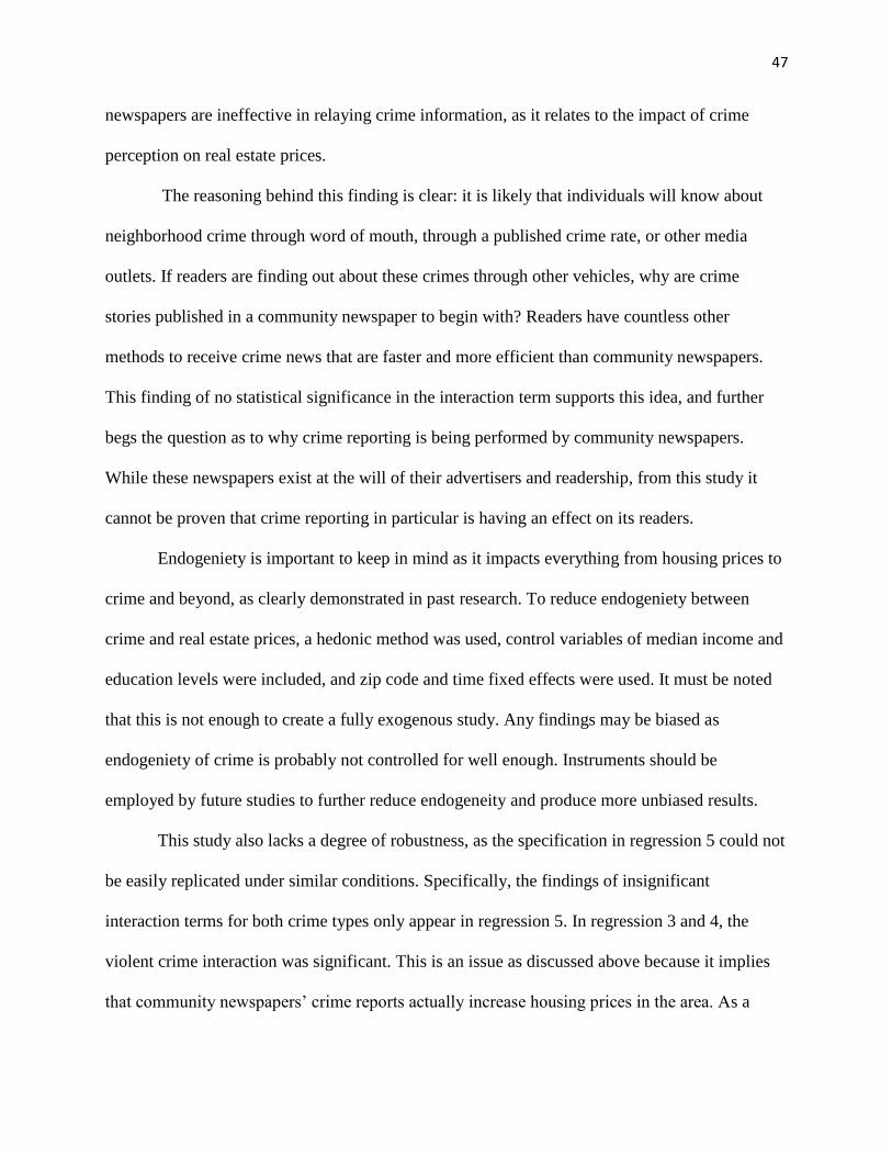
47

newspapers are ineffective in relaying crime information, as it relates to the impact of crime

perception on real estate prices.

The reasoning behind this finding is clear: it is likely that individuals will know about

neighborhood crime through word of mouth, through a published crime rate, or other media

outlets. If readers are finding out about these crimes through other vehicles, why are crime

stories published in a community newspaper to begin with? Readers have countless other

methods to receive crime news that are faster and more efficient than community newspapers.

This finding of no statistical significance in the interaction term supports this idea, and further

begs the question as to why crime reporting is being performed by community newspapers.

While these newspapers exist at the will of their advertisers and readership, from this study it

cannot be proven that crime reporting in particular is having an effect on its readers.

Endogeniety is important to keep in mind as it impacts everything from housing prices to

crime and beyond, as clearly demonstrated in past research. To reduce endogeniety between

crime and real estate prices, a hedonic method was used, control variables of median income and

education levels were included, and zip code and time fixed effects were used. It must be noted

that this is not enough to create a fully exogenous study. Any findings may be biased as

endogeniety of crime is probably not controlled for well enough. Instruments should be

employed by future studies to further reduce endogeneity and produce more unbiased results.

This study also lacks a degree of robustness, as the specification in regression 5 could not

be easily replicated under similar conditions. Specifically, the findings of insignificant

interaction terms for both crime types only appear in regression 5. In regression 3 and 4, the

violent crime interaction was significant. This is an issue as discussed above because it implies

that community newspapers’ crime reports actually increase housing prices in the area. As a

48

result, regression 5 was the most sensible to use in terms of the variables of note. Though this

non-significant interaction finding was not able to be replicated consistently, regression 5 still

results in the most believable of any alternative, as it removed issues with the variables of note

and produced logical and believable results.

An easy way to improve robustness for future studies is to refine the income control

variable. Findings in this project were questionable due to imputation methods. IRS tax income

information may improve specification robustness. Increasing robustness through income and

using an instrument would go a long way towards increasing this study’s reliability of results,

and hopefully would result in regressions that display sensible interaction term coefficients.

As mentioned above, confirmation bias is a worry here. However, it is mitigated because

the regression selected is simply the only one with sensible coefficients on the variables of note.

This study was not rejecting regressions out of hand because they did not agree with a

hypothesis. Rather, it rejected results if they did not align with common sense. While the

regressions rejected certainly may have some merit, a positive sign on the interaction terms

implies some type of bias in the results. Because of this lack of reasonable alternatives,

regression 5 was selected.

An accurate, unbiased finding that community newspapers are ineffective in delivering

crime news raises the question as to why these papers are reporting on crime. It cannot be proven

here that this type of reporting is successfully increasing individuals’ perception of crime in their

neighborhood as this perception relates to housing prices. The question, then, is why community

newspapers are printing crime news at all. Their delivery is slower, their resources are fewer, and

the platform is far more rigid than online competitors. Why print a crime story in a local paper at

all if it is not impacting the readership's awareness of crime?

49

Community newspapers may have some other benefits besides raising awareness of

crime, and these aspects are not able to be estimated in this study. For example, community

papers may prevent corruption in local politics due to the threat that this corruption would be

reported. This preventative type of benefit is not tracked through the regression study used here.

Still, if an increase in crime perception is not resulting from reading a community newspaper,

regardless of who is doing the reading, it must be asked why these stories are printed in the first

place. I hope that this research will serve as springboard for future projects in which the true

value of crime reporting, and community newspapers in general, is ascertained.

While it is impossible to make sweeping findings from just one study, I hope to be able to

begin an ongoing discussion as to the true reasoning behind the existence of community

newspapers. Community newspapers are a conundrum as they are an expensive, glacially paced

reporting method in our high-strung instant gratification lifestyle. This preliminary study shows

that crime reporting by community newspapers cannot be proven effective. Building on the

research I have done into the effectiveness of reporting on crime news will lead to more

complete conclusions on the overall purpose of community newspapers. I hope starting this

conversation will lead to more attention to the issue and conclusive results in the near future.

50

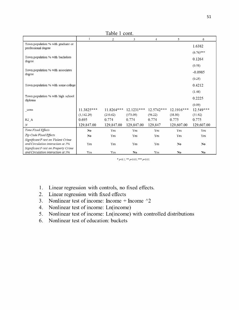
51

52

53

54

55

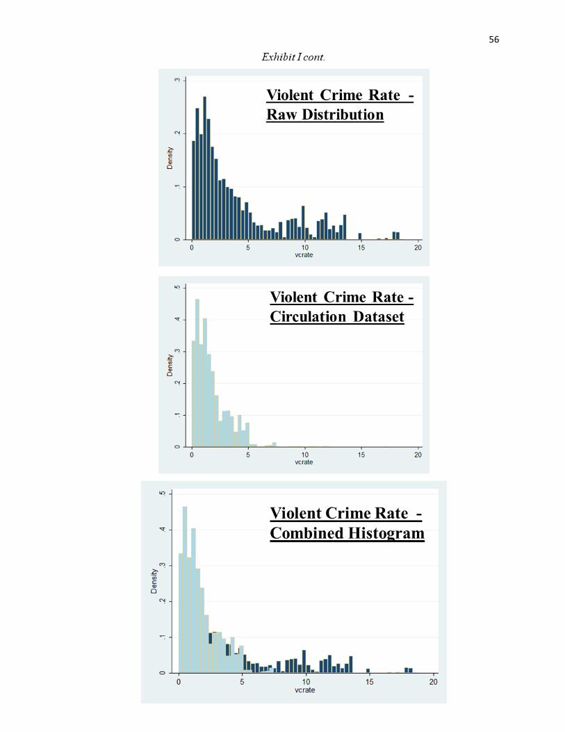
56

57

58

59

References

Bowes, David R. & Ihlanfeldt, Keith R., 2001. "Identifying the Impacts of Rail Transit Stations

on Residential Property Values," Journal of Urban Economics, Elsevier, vol. 50(1), pages 1-25,

July.

Karl E. Case & Christopher J. Mayer, 1995. "Housing price dynamics within a metropolitan

area," Working Papers 95-3, Federal Reserve Bank of Boston.

Schwartz, Amy Ellen, Scott Susin, and Ioan Voicu. "Has falling crime driven New York City's

real estate boom?." Journal of Housing Research 14.1 (2003): 101-136.

Linden, Leigh, and Jonah E. Rockoff. "Estimates of the Impact of Crime Risk on Property

Values from Megan's Laws." The American Economic Review 98.3 (2008): 1103-1127.

Petras, Tricia L. Measuring the effects of perceptions of crime on neighborhood quality and

housing markets. Diss. The Ohio State University, 2007.

Keith Ihlanfeldt &Tom Mayock. Crime and Housing Prices Department of Economics and

DeVoe Moore Center. Florida State University, 2009.

Dugan, Laura. "THE EFFECT OF CRIMINAL VICTIMIZATION ON A HOUSEHOLD'S

MOVING DECISION*." Criminology 37.4 (1999): 903-930.

George, Lisa M., and Joel Waldfogel. "The New York Times and the market for local

newspapers." The American economic review 96.1 (2006): 435-447.

Gentzkow, Matthew, Jesse M. Shapiro, and Michael Sinkinson. The effect of newspaper entry

and exit on electoral politics. No. w15544. National Bureau of Economic Research, 2009.

Fan, Ying. "Ownership Consolidation and Product Characteristics: A Study of the U.S. Daily

Newspaper Market", American Economic Review, forthcoming, 2012.

Hendel, John H, and David N. Atkinson. The Birth of Freedom of the Press in America. , 1999.

Print.

Acknowledgements

60

I would like to profusely thank my primary advisor, Professor Davide Pettenuzzo.

Without his (sometimes more than) weekly guidance, this project would never have

gotten off the ground and certainly would not be what it is today.

I would like to thank my secondary advisor, Professor Benjamin Shiller. His expertise

and creative suggestions take this thesis to the next level, both intuitively and creatively.

I would like to thank my outside reader, Professor Maura Jane Farrelly. Her agreement to

be my reader and journalistic advice convinced me to write on this topic.

I would like to thank Roxanne Pacella for her preposterous patience and helpfulness in

guiding me on how to obtain real estate data.

I would definitely like to thank my team of arduous proofreaders, in order of first name,

without whom this thesis would be filled with words like arduous:

o Gabrielle Katz

o Madeline Katz

o Nina Godles

o Natalie Light

Finally, a big thank you to the Economics department and faculty. Particularly, to the

thesis program coordinator, Professor Brainerd, the Economics department chair,

Professor Graddy, for their early and ongoing advice. Also, thank you to Meredith

Robitaille for answering all of my scheduling questions and being generally great.