Expository Notes on Introduction to Harmonic

Analysis

Matthew Begue

December 18, 2012

The following contains results with explanations from Yitzhak Katznelson’sAn Introduction to Harmonic Analysis [Katz]. I present some of the results withKatznelson’s proof often with expanded details. In some cases, I even providealternate proofs to some of the results.

1 Fourier Analysis on T1.1 Preliminaries

The group T is defined as the quotient R/2πZ. There is a clear identificationbetween functions on T and 2π-periodic functions on R. This periodicity prop-erty gives us translation invariance of the integral. That is, for every t0 ∈ T andf defined on T we have ∫

Tf(t− t0) dt =

∫Tf(t) dt.

We denote the L1 norm on T as follows: for f ∈ L1(T) we let

||f ||L1(T) =1

2π

∫T|f(t)| dt.

It is well-known that L1(T) is a Banach space.Let f ∈ L1(T). We define the nth Fourier coefficient by

f(n) =1

2π

∫Tf(t)e−int dt.

The following are some elementary properties of Fourier coefficients:

Theorem 1.1. For f, g ∈ L1T then

1. (f + g)(n) = f(n) + g(n).

2. For any α ∈ C, (αf)(n) = αf(n).

3. Let f denote the complex conjugate of f . Then ˆf(n) = f(n).

4. For x ∈ T let (τxf)(t) = f(t− x). Then τxf(n) = f(n)e−inx.

1

5.

(1.1) |f(n)| ≤ ‖f‖L1T .

6. Assume f, f ′ ∈ L1(T) and f(0) = 0. Then for n 6= 0, f(n) = 1in f′(n).

Proof. Parts 1 and 2 follow immediately from linearity and homogeneity of theintegral. Parts 3 and 4 follow from the definition of the Fourier coefficients off . Part 5 follows since

|f(n)| = | 1

2π

∫Tf(t)e−int dt| ≤ 1

2π

∫T|f(t)e−int| dt = ‖f‖L1(T) .

For Part 6 we take the definition of f(n) and integrate by parts to obtain

2πf(n) =

∫ 2π

0

f(t)e−int dt = f(t)e−int

−in

∣∣∣∣2π0

−∫ 2π

0

f ′(t)e−int

−indt =

2π

inf ′(n).

Notice that the periodicity of f ∈ L1(T) was explicitly used to make boundaryterms vanish.

Theorem 1.2. [The Riemann-Lebesgue Lemma] Let f ∈ L1(T), then lim|n|→∞ f(n) =0.

Lebesgue-Riemann Theorem Proof 1. This is the proof given in [Katz]. First,recall that trigonometric polynomials on T are dense in L1(T). That is, forε > 0 there exists a trigonometric polynomial P such that ‖f − P‖L1(T) < ε. If

|n| > degP then

|f(n)| = |f(n)− 1

2π

∫TP (t)e−int dt| = | (f − P )(n)|

The integral above is equal to 0 since |n| > degP and∫T e−ikt dt = 0 for any

k 6= 0. This gives |f(n)| = | (f − P )(n)| ≤ ‖f − P‖L1(T) < ε by (1.1).

Lebesgue-Riemann Theorem Proof 2. Let 1A denote the indicator function ofthe Lebesgue measurable set A. Suppose A = [−c, c] is a closed interval sym-metric about the origin. Then the Fourier coefficients of 1[−c,c] are:

1[−c,c] =1

2π

∫T1[−c,c]e

−int dt =1

2π

∫ c

−ce−int dt

=e−int

−2πin

∣∣∣∣c−c

=1

−πne−inc − einc

2i=

sin(−nc)−πn

=sin(nc)

πn.

Then by Theorem 1.1, we can write the Fourier coefficients of the indicatoron any interval as:

1[a,b](n) =(

τ b+a21[− b−a2 , b−a2 ]

)(n) = e(−in

b+a2 ) sin(n b−a2 )

πn.

Then for any α ∈ R we see that

lim|n|→∞

∣∣∣ (α1[a,b])(n)∣∣∣ ≤ lim

|n|→∞

α

πn= 0.

2

Then for any simple function (i.e. finite linear combination of indicator

functions), ϕ(t) =

N∑i=1

αi1Ii(t) then ϕ(n)→ 0 as |n| → ∞.

Simple functions are dense in L1(T); that is, given f ∈ L1T and ε > 0 thereexists a simple ϕ(t) such that ‖f − ϕ‖L1(T) < ε. Then by the triangle inequalityand Theorem 1.1 we have∣∣∣|f(n)| − |ϕ(n)|

∣∣∣ ≤ |f − ϕ(n)| ≤ ‖f − ϕ‖L1(T) < ε.

This implies that lim|n|→∞ |f(n)| < ε which proves the theorem.

Lebesgue-Riemann Theorem Proof 3. Yet another way to prove the Lebesge-Riemann Theorem is to study functions in C1

C(T), that is, functions on T witha continuous first derivative and that vanish at zero. Let g ∈ C1

C(T). Then wecan integrate by parts to obtain

g(n) =1

2π

∫Tg(t)e−int dt

=1

2π

[0 +

∫Tg′(t)

eint

indt

].

There are no boundary terms since we chose g to vanish at 0. Then we canestimate

|g(n)| ≤[∫

T

∣∣∣∣g′(t)eintin∣∣∣∣ dt]

≤ maxt∈[0,2π)

|g′(t)| 1

|n|→ 0 as |n| → ∞.

Note that C1c (T) is also dense in L1(T). Therefore, for any f ∈ L1T and

ε > 0 there exists a g(t) ∈ C1c (T) such that ‖f − g‖L1(T) < ε. Then by the

triangle inequality and Theorem 1.1 we have∣∣∣|f(n)| − |g(n)|∣∣∣ ≤ |f − g(n)| ≤ ‖f − g‖L1(T) < ε.

This implies that lim|n|→∞ |f(n)| < ε which proves the theorem.

Definition 1.3. For f, g ∈ L1(T) we define the convolution f ∗ g as f ∗ g(t) =12π

∫T f(t− x)g(x) dx.

The following theorem contains standard properties about the convolutionwhich we provide without proof at this time:

Theorem 1.4. For f, g ∈ L1(T), then the following properties hold:

(a) f(t− τ)g(τ) is integrable as a function of τ ∈ T.

(b) ‖f ∗ g‖L1(T) ≤ ‖f‖L1(T) ‖g‖L1(T).

(c) The convolution operation in L1(T) is commutative (i.e. f ∗ g = g ∗ f).

(d) f ∗ g(n) = f(n)g(n) for all integers n.

3

1.2 Summability Kernels

Definition 1.5. A summability kernel is a sequence {kn} of continuous func-tions on T (hence 2π-periodic) satisfying:

1. 12π

∫T kn(t) dt = 1

2. 12π

∫T |kn(t)| dt ≤ C

3. For all 0 < δ < π, limn→∞∫ 2π−δδ

|kn(t)| dt = 0.

That is, a summability kernel is a sequence of functions that integrate to one,are uniformly bounded in the L1 norm, and integrate to 0 off of a neighborhoodabout 0.

The following is of great importance and makes summability kernels ex-tremely useful to study:

Theorem 1.6. For f ∈ L1(T) and {kn} any summability kernel, then

limn→∞

‖f − kn ∗ f‖L1(T) = 0.

1.2.1 Fejer Kernel

One of the best known summability kernels is the Fejer kernel defined by

(1.2) Kn(t) =

n∑j=−n

(1− |j|

n+ 1

)eijt.

Before we show that {Kn(t)} is a summability kernel, the following Lemmais useful.

Lemma 1.7. Kn(t) = 1n+1

[sin(n+1

2 t)sin(t/2)

]2.

Proof. Recall the following trigonometric identity: sin2(t/2) = 1/2(1−cos(t)) =

1/2 − e−it+eit

4 (where the last equality comes from Euler’s formula cos(t) =1/2(eit + e−it)).

Then

sin2(t/2)Kn(t) =

(1/2− e−it + eit

4

) n∑j=−n

(1− |j|

n+ 1

)eijt

=1

n+ 1

(1/2− e−i(n+1)t + ei(n+1)t

4

)=

1

n+ 1sin2

(n+ 1

2t

)which proves the desired equality.

Notice that one result of Lemma 1.7 is that Kn(t) is a positive summabilitykernel (i.e. Kn(t) ≥ 0 for all n and for all t ∈ T).

Theorem 1.8. The Fejer kernel {Kn} is a summability kernel.

4

Proof. We need to verify the three conditions given in Definition 1.5. Firstly,

1

2π

∫TKn(t) dt =

1

2π

∫T

n∑j=−n

(1− |j|

n+ 1

)eijt dt

=1

2π

n∑j=−n

(1− |j|

n+ 1

)∫Teijt dt

This integral is zero for all values of j except for j = 0. Thus

1

2π

∫TKn(t) dt =

1

2π

(1− |0|

n+ 1

)∫T

1 dt = 1.

The second property follows immediately from the first since Lemma 1.7tells us that {Kn(t)} is a positive summability kernel (i.e. |Kn(t)| = Kn(t) forall t ∈ T and for all n). Moreover, this tells us that ‖Kn‖L1(T) = 1 for all n.

The third condition also follows from Lemma 1.7 since∫ 2π−δ

δ

|Kn(t)| dt =

∫ 2π−δ

δ

∣∣∣∣∣∣ 1

n+ 1

[sin(n+12 t)

sin(t/2)

]2∣∣∣∣∣∣ dt≤ 1

n+ 1

∫ 2π−δ

δ

[1

sin(δ/2)

]2dt→ 0 as n→∞.

Figure 1 shows the graphs of Kn(t) for a few choices of n. The figures clearlyexhibit the positivity and delta-like behavior as n grows.

We will need the Fourier coefficients of the Fejer kernel for proofs in thesubsequent sections.

Proposition 1.9.

Kn(m) =

{ (1− |m|

n+1

)if n ≥ |m|

0 otherwise

Proof. By definition of Fourier coefficients, we have

Kn(m) =1

2π

∫T

n∑j=−n

(1− |m|

n+ 1

)ei(j−m)t dt

=1

2π

n∑j=−n

(1− |m|

n+ 1

)∫Tei(j−m)t dt.

The integral∫T e

i(j−m)t dt equals 0 if j 6= m and equals 2π only if j = m. Thus

Kn(m) =

(1− |m|

n+ 1

)provided n ≥ |m|.

5

Figure 1: Plots of the Fejer kernel Kn(t) on t ∈ [−π, π] for n = 1, 5, 10, 50.

1.2.2 Dirichlet Kernel

Another important function is the Dirichlet kernel defined by

(1.3) Dn(t) =

n∑j=−n

eijt =sin((n+ 1/2)t)

sin(t/2).

Figure 2 shows the graphs of Dn(t) for a few choices of n. The figures clearlyexhibit the positivity and delta-like behavior as n grows.

Remark 1.10. It is important to note that the Dirichlet kernel is not a summa-bility kernel.

Proof. The Dirichlet kernel does satisfy condition 1 in Definition 1.5; that is,

1

2π

∫T

n∑j=−n

eijt dt = 1

since each of the 2n+ 1 integrals equal zero except when j = 0.However Dn(t) does not satisfy condition number 2 or 3. · · ·

1.2.3 Homogeneous Banach Spaces

Definition 1.11. A homogeneous Banach space on T is a linear subspace B ofL1(T) that is Banach under the norm ‖·‖B ≥ ‖·‖L1(T) with the following twoproperties:

6

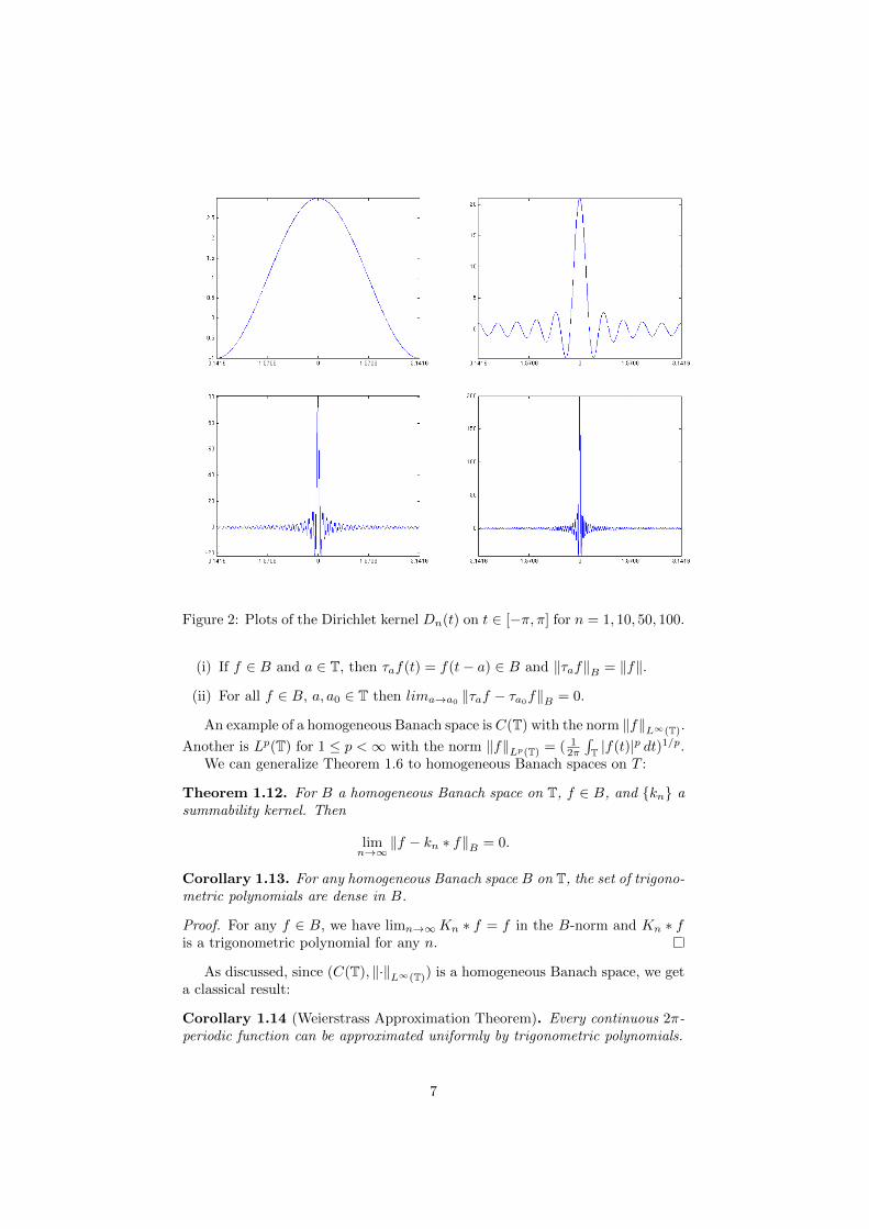
Figure 2: Plots of the Dirichlet kernel Dn(t) on t ∈ [−π, π] for n = 1, 10, 50, 100.

(i) If f ∈ B and a ∈ T, then τaf(t) = f(t− a) ∈ B and ‖τaf‖B = ‖f‖.

(ii) For all f ∈ B, a, a0 ∈ T then lima→a0 ‖τaf − τa0f‖B = 0.

An example of a homogeneous Banach space is C(T) with the norm ‖f‖L∞(T).

Another is Lp(T) for 1 ≤ p <∞ with the norm ‖f‖Lp(T) = ( 12π

∫T |f(t)|p dt)1/p.

We can generalize Theorem 1.6 to homogeneous Banach spaces on T :

Theorem 1.12. For B a homogeneous Banach space on T, f ∈ B, and {kn} asummability kernel. Then

limn→∞

‖f − kn ∗ f‖B = 0.

Corollary 1.13. For any homogeneous Banach space B on T, the set of trigono-metric polynomials are dense in B.

Proof. For any f ∈ B, we have limn→∞Kn ∗ f = f in the B-norm and Kn ∗ fis a trigonometric polynomial for any n.

As discussed, since (C(T), ‖·‖L∞(T)) is a homogeneous Banach space, we geta classical result:

Corollary 1.14 (Weierstrass Approximation Theorem). Every continuous 2π-periodic function can be approximated uniformly by trigonometric polynomials.

7

Exercise 1.15 (Katznelson 1.2.13). Let B be a homogeneous Banach space onT. Show that if g ∈ L1(T) and f ∈ B then g ∗ f ∈ B and

(1.4) ‖g ∗ f‖B ≤ ‖g‖L1(T) ‖f‖BSolution. Suppose first, that g is continuous on T. Then

‖g ∗ f‖B =1

2π

∥∥∥∥∫Tg(τ)f(t− τ) dτ

∥∥∥∥B

≤ 1

2π

∫T‖g(τ)f(t− τ)‖B dτ

=1

2π

∫T|g(τ)| ‖f(t− τ)‖B dτ =

1

2π

∫T|g(τ)| ‖f(t)‖B dτ

= ‖g‖L1(T) ‖f‖B .

In the case where g is not continuous, we use Theorem 1.12 and its corollariesto approximate g by Kn ∗ g.

1.3 Order of Magnitude of Fourier Coefficients

Thus far we’ve established two immediate facts about the magnitude of f(n).

Given f ∈ L1(T) we have |f(n)| ≤ ‖f‖L1(T) for all n and lim|n|→∞ |f(n)| = 0by the Riemann-Lebesgue Theorem.

Some natural questions arise. The first question is: Can we get an estimateof the rate of vanishing of |f(n)|? The answer to this is no. In the followingtheorem, we show that there exist functions whose Fourier coefficients decay tozero arbitrarily slow.

Theorem 1.16. Let {an}n∈N be an even sequence of nonnegative numbers tend-ing to 0. Assume that {an} is a convex sequence (i.e. an−1 + an+1 − 2an ≥ 0

for all n). Then there exists a nonnegative f ∈ L1(T) such that f(n) = an.

Proof. The convexity condition gives us that an−1 − an ≥ an − an+1, that is,{an − an+1} is a sequence of positive numbers monotonically decreasing to 0.

We claim, next, that limn→∞ n(an − an+1) = 0. To see this, observe firstthat since limn→∞ an = 0, given any ε > 0 there exists some N > 0 such that forall n > N we have an < ε. Since the sequence {an} is positive and decreasing,then an − an+k < ε/2 for any n > N and k ∈ N. We can write this quantity asthe telescoping sum

an − an+k =

k∑i=1

an+i−1 − an+i ≤ k(an+k−1 − an+k)

since (an+k−1 − an+k) ≤ (an+i−1 − an+i) for every i = 1, ..., k. Now let n > Nbe fixed and perform a change of variables; let m = n+ k − 1. Then we have

(m+ (−n+ 1))(am − am+1) < ε/2.

Rearranging gives

m(am − am+1) < ε/2 + (n− 1)(am − am+1).

Since {am−am+1} → 0 there exists an M > 0 such that for all m > M we have(n− 1)(am − am+1) < ε/2. Thus for picking n > N and then m > M we havem(am − am+1) < ε. Hence

(1.5) limn→∞

n(an − an+1) = 0

8

as desired.Now consider the following series:

N∑n=1

n(an−1 + an+1 − 2an)

= a0 + a2 − 2a1 + 2a1 + 2a3 − 4a2 + 3a2 + 3a4 − 6a3 + · · ·+(N − 1)(aN−2 + aN − 2aN−1) +N(aN−1 + aN+1 − 2aN )

= a0 + (N − 1)aN +N(aN+1 − 2aN )

= a0 − aN +N(aN+1 − aN )

As we letN →∞, the second and third terms vanish by (1.5). Thus limN→∞

N∑n=1

n(an−1+

an+1 − 2an) = a0.Now consider the function

f(t) =

∞∑n=1

n(an−1 + an+1 − 2an)Kn−1(t)

where Kn(t) =

n∑j=−n

(1− |j|n+ 1

)eijt is the Fejer kernel.

We claim that f ∈ L1(T). To see this, consider the sequence of functions

fN (t) =

N∑n=1

n(an−1 + an+1 − 2an)Kn−1(t). Each fN ∈ L1(T) since

‖fN‖L1(T) =

N∑n=1

n(an−1 +an+1−2an) ‖Kn−1‖L1(T) =

N∑n=1

n(an−1 +an+1−2an)

since ‖Kn‖L1(T) = 1 for all n by 1.8. Furthermore, each fN converges pointwise

to some function f . To see this we use the form of Kn(t) given by Lemma 1.7to get:

limN→∞

fN (t) = limN→∞

N∑n=1

n(an−1 + an+1 − 2an)1

n

1

sin(1/2t)2sin

(nt

2

)2

≤ limN→∞

N∑n=1

n(an−1 + an+1 − 2an)1

sin(1/2t)2= a0

1

sin(1/2t)2

which is finite a.e. on T.In addition, by Lemma 1.7 we see that Kn(t) is a positive kernel. Thus,fN ≤

fN+1 for all N . Then we can apply the Lebesgue Monotone Convergence The-orem (Beppo Levi) to conclude that limN→∞

∫fN =

∫f . Thus, ‖f‖L1(T) =

∞∑n=1

n(an−1 + an+1 − 2an) = a0 <∞.

Since f ∈ L1(T), we can now compute its Fourier coefficients (using Propo-

9

sition 1.9):

f(j) =

∞∑n=1

n(an−1 + an+1 − 2an)Kn−1(j)

=

∞∑n=|j|+1

n(an−1 + an+1 − 2an)(1− |j|n

)

=

∞∑n=|j|+1

(n− |j|)(an−1 + an+1 − 2an).

Every term in this series cancels except for the first, a|j|.Thus, given any even convex sequence {an}n∈N that tends to zero (arbitrarily

slowly), we can construct a function f ∈ L1(T) such that f(j) = aj for everyinteger j.

We will show (in Proposition 1.32) that a sequence {bn} ∈ `1(R) is theFourier coefficients of a function in L1(T). Sequences in `1(R) necesarilly tendto zero and can do so arbitrarily slowly. This provides an alternate proof showingthat we cannot estimate the rate of vanishing of Fourier coefficients. Howeverthe proof given is stronger since the set of convex sequences vanishing are propersubset of `1

Example 1.17. Show a convex sequence of numbers that is not in `1. Considerthe real function f(x) = 1

log(|x|+2) . Clearly f(x) is positive and tends to infinity

as |x| → ∞. This function is also convex (since f ′′(x) = 2(2+x)2 log(2+x)3 +

1(2+x)2 log(2+x)2 ≥ 0) but is not in L1(R), i.e.

∫R

1log(|x|+2) dx diverges. Now

consider the sequence of real numbers {an}n∈N defined by an = f(n). Thesequence clearly tends to 0 as |n| → ∞ and the convexity follows from theconvexity of f . But by the integral convergence test for series, {an} /∈ `1.

Thus far, we have demonstrated that convex sequences that tend to zero arethe Fourier coefficients of some function f ∈ L1(T) (We also mentioned that thesame is true for equences in `1). But is it true that any sequence {an} whichtends to zero is the Fourier coeffieicents of some f ∈ L1(T)? The answer tothis question is no. This can be proved with the contrapositive of the followingtheorem:

Theorem 1.18. Assume f ∈ L1(T) and f(|n|) = −f(−|n|) ≥ 0. Then∑n 6=0

1

nf(n) <∞.

Proof. Define the function F (t) =∫ t0f(τ) dτ . By construction, F (t) is (abso-

lutely) continuous. Then by Theorem 1.1 F (n) = 1in f(n) for any n 6= 0. Since

F is continuous, then by Fejer’s Theorem ?? at t = 0,

limN→∞

KN ∗ F (0) =

N∑j=−N

(1− |j|

N + 1

)F (j)eij0

= limN→∞

F (0) + 2

N∑j=1

(1− |j|

N + 1

)1

ijf(j) = F (0)

10

This gives ∑j 6=0

f(j)

j= i(F (0)− F (0)).

which proves the theorem.

The answer to our question is the contrapositive of the above theorem. Thatis,

Corollary 1.19. If an > 0 and∑n 6=0

ann = ∞. Then

∞∑n=1

an sin(nt) is not a

Fourier series.

In other words, arbitrary sequences that decay to zero are not necessarilythe Fourier coeffieicents of an L1 function.

A third natural question to ask is: How does smoothness affect the decay off(n)?

Theorem 1.20. If f ∈ L1(T) is absolutely continuous, then f(n) = o(1/n).

Proof. Again, by Theorem 1.1 we have f(n) = 1in f′(n). The Riemann-Lebesgue

lemma (Theorem 1.2) says that f ′(n) → 0 as n → ∞. This tells us that

f(n) = o(1/n).

Suppose instead f ∈ Ck(T) and f (k) ∈ L1(T) then we can conclude that

f(n) = o(1/nk) by following the proof above with repeated integration by parts.

Theorem 1.21. If f ∈ BV (T), then f(n) ≤ Var(f)2π|n| .

Proof. We have |f(n)| =∣∣ 12π

∫T f(t)e−int dt

∣∣ and integrating by parts gives

|f(n)| =∣∣∣∣ 1

2πin

∫Te−intf ′(t) dt

∣∣∣∣ ≤ 1

2π|n|

∫T|f ′(t) dt| = Var(f)

2π|n|.

11

1.4 Fourier Series of Square Summable Functions

This section corresponds to Section 1.5 of [Katz].Let H be a complex Hilbert space, i.e. a complex inner product space that

is complete with respect to the norm induced by the inner product. The normof f ∈ H is defined as ‖f‖ = (〈f, f〉)1/2. We say that f, g ∈ H are orthogonalif the inner product 〈f, g〉 = 0. The function f ∈ H is orthogonal to the setE ⊆ H if f is orthogonal to each element of E. The set E ⊆ H is orthogonal ifany two elements of E are orthogonal. The set E ⊆ H is orthogonormal if it isorthogonal and the norm of each vector is 1.

Theorem 1.22. Let {ϕn}∞n=1 be an orthonormal system in H and let {an}∞n=1 ∈`2, i.e.

∑∞n=1 |an|2 <∞. Then

∑∞n=1 anϕn converges in H.

Proof. First notice that for any finite subset of {ϕn} we have∥∥∥∥∥N∑n=1

anϕn

∥∥∥∥∥2

=

⟨N∑n=1

anϕn,

N∑j=1

ajϕj

⟩, by definition of norm on H

=

N∑n=1

an

⟨ϕn,

N∑j=1

ajϕj

⟩, by linearity of the inner product

=

N∑n=1

N∑j=1

anaj 〈ϕn, ϕj〉 , also by linearity of the inner product

=

N∑n=1

anan =

N∑n=1

|an|2 by the orthogonality of{ϕn}Nn=1.

Because Hilbert spaces are complete, it suffices to show that the partial sumsSN =

∑Nn=1 anϕn form a Cauchy sequence in H. For any N,M > 0 we have

‖SN − SM‖2 =

N∑n=M+1

|an|2.

Since {an} ∈ `2, for any ε > 0 we can select Nε > 0 so that∑∞n=Nε

|an|2 < εwhich gives us that the above equation is also less than epsilon for N,M > Nε.Thus SN is Cauchy in H and thus converges in H by completeness.

Lemma 1.23 (Bessel’s Inequality). Let {ϕα} be an orthonormal system inHilbert space H. For f ∈ H define aα = 〈f, ϕα〉. Then

(1.6)∑α

|aα|2 ≤ ‖f‖2 .

Proof. First, suppose that {ϕn}Nn=1 is a finite orthonormal system. Then by the

12

definition of the H-norm and linearity of the inner product:

0 ≤

∥∥∥∥∥f −N∑n=1

anϕn

∥∥∥∥∥2

=

⟨f −

N∑n=1

anϕn, f −N∑j=1

ajϕj

⟩

=

⟨f, f −

N∑j=1

ajϕj

⟩+

N∑n=1

an

⟨ϕn, f −

N∑j=1

ajϕj

⟩

= 〈f, f〉 −N∑j=1

aj〈f, ϕj〉+

N∑n=1

an〈ϕn, f〉 −N∑n=1

N∑j=1

anaj〈ϕn, ϕj〉

= 〈f, f〉 −N∑j=1

ajaj +

N∑n=1

anan −N∑n=1

anan

= ‖f‖2 −N∑n=1

|an|2

which proves (1.6) for the case where our orthonormal system is finite. Sup-pose now that {ϕα} is infinite (countable or uncountable) and that (1.6) doesnot hold. Then there must exist some finite subcollection of {ϕα} for which∑α

|aα|2 > ‖f‖2, which is a clear contradiction.

Definition 1.24. An orthonormal system {ϕα} in H is said to be completeprovided that the only vector in H orthogonal to it is the zero vector.

Lemma 1.25. Let {ϕn} be an orthonormal system in H. Then the followingare equivalent:

(a) {ϕn} is complete.

(b) For every f ∈ H we have ‖f‖2 =∑n

|〈f, ϕn〉|2 .

(c) For every f ∈ H we have f =∑n

〈f, ϕn〉ϕn.

Proof. (a ⇒ c): Let {ϕn} be an orthonormal complete system and let f ∈ H.

By Bessel’s Inequality,∑n |〈f, ϕn〉|2 ≤ ‖f‖

2< ∞. Then by Theorem 1.22,∑

n〈f, ϕn〉ϕn converges in H to some function g ∈ H. Notice now that

〈g, ϕn〉 =

⟨∑j

〈f, ϕj〉ϕj , ϕn

⟩=∑j

〈f, ϕj〉〈ϕj , ϕn〉 = 〈f, ϕn〉.

Thus, by linearity, f − g ∈ H is orthogonal to ϕn. Since {ϕn} is complete, thismeans that f − g = 0. That is, f =

∑n〈f, ϕn〉ϕn.

13

(c⇒ b): Assume f =∑n〈f, ϕn〉ϕn. Then

‖f‖2 = 〈f, f〉 =

⟨∑n

〈f, ϕn〉ϕn,∑j

〈f, ϕj〉ϕj

⟩=

∑n

∑j

〈f, ϕn〉〈f, ϕj〉〈ϕn, ϕj〉

=∑n

〈f, ϕn〉〈f, ϕn〉 =∑n

|〈f, ϕn〉|2.

(b ⇒ a): If f is orthogonal to all of {ϕn}, i.e. if 〈f, ϕn〉 = 0 for all n, thenby assumption (b),

‖f‖2 =∑n

|〈f, ϕn〉|2 = 0.

Since ‖ · ‖ is a norm on H, then ‖f‖ = 0 if and only if f = 0. Thus, {ϕn} iscomplete.

Exercise 1.26 (Katznelson 1.5.1). Let {ϕn} be an orthogonal system in a

Hilbert space H. Let f ∈ H. Show that

∥∥∥∥∥∥f −N∑j=1

ajϕj

∥∥∥∥∥∥ achieves a minimum at

the point aj = 〈f, ϕj〉 for j = 1, 2, ..., N and only there.

Solution. : We can write

f −N∑j=1

ajϕj = f −N∑j=1

〈f, ϕj〉ϕj +

N∑j=1

cjϕj

where cj = 〈f, ϕj〉 − aj . Then by the triangle inequality,∥∥∥∥∥∥f −N∑j=1

ajϕj

∥∥∥∥∥∥ ≤∥∥∥∥∥∥f −

N∑j=1

〈f, ϕj〉ϕj

∥∥∥∥∥∥+

∥∥∥∥∥∥N∑j=1

cjϕj

∥∥∥∥∥∥ .Then, since {ϕ} is an orthogonal system, the last norm will equal zero if andonly if cj = 0 for all j = 1, 2, ..., N .

1.4.1 The Hilbert space L2(T)

It is known that Lp(T) are complete for all 1 ≤ p ≤ ∞ (by the Riesz-FischerTheorem). However, only L2(T) is a Hilbert space because it is equipped withthe inner product 〈f, g〉 = 1

2π

∫T f(t)g(t) dt.

Proposition 1.27. For H = L2(T), the exponentials {eint}∞n=−∞ form a com-plete orthonormal system.

Proof. Orthonormality follows easily since

〈eint, eimt〉 =1

2π

∫Tei(n−m)t dt = δn,m.

If f is continuous, then we can approximate f in L2 by trigonometric poly-nomials. That is, for any small ε > 0 there exists a trigonometric polynomial

14

P of degree N such that ‖f − P‖L2(T) < ε. Then by Exercise 1.26 we also get∥∥∥f −∑Nn=−N f(n)eint

∥∥∥L2(T)

< ε. This verifies condition (b) of Lemma 1.25.

Suppose f ∈ L2(T) is not continuous. We can approximate f in the L2 normby a continuous function. That is, for ε > 0 there exists a g ∈ C(T) such that

‖f − g‖L2(T) < ε/3. (For sake of notation let SN (f) =

N∑n=−N

f(n)eint) Then

‖f − SN (f)‖L2(T) ≤ ‖f − g‖L2(T) + ‖g − SN (g)‖L2(T) + ‖SN (g)− SN (f)‖L2(T) .

Look at the three terms on the left hand side. By our choice of g, the first termis less than ε/3. By the previous argument, the second term is less than ε/3 forN sufficiently large. As for the third term,

‖SN (g)− SN (f)‖L2(T) = ‖SN (g − f)‖L2(T)

=

(1

2π

∫T|

N∑n=−N

(g − f)(n)eint|2 dt

)1/2

=

N∑n=−N

| (g − f)(n)|2

≤ ‖f − g‖2L2(T) < ε2/9

where the last inequality follows from Bessel’s inequality. Therefore we’ve shown

that

∥∥∥∥∥f −N∑

n=−Nf(n)eint

∥∥∥∥∥L2(T)

≤ ε/3 + ε/3 + ε2/9 < ε which verifies condition

(b) in Lemma 1.25.

Theorem 1.28. Let f ∈ L2(T). Then

(a)∑n

|f(n)|2 =1

2π

∫|f(t)|2 dt.

(b) f = limN→∞

N∑n=−N

f(n)eint in the L2(T) norm.

(c) Given any complex sequence {an}∞n=−∞ ⊂ `2(C), there exists a unique f ∈L2(T) such that an = f(n).

(d) Let f, g ∈ L2(T). Then

1

2π

∫f(t)g(t) dt =

∞∑n=−∞

f(n)g(n).

Proof. (a): We have just shown that {eint} is a complete orthonormal systemin L2(T). Then the statement (a) of Theorem 1.28 is precisely statement (b)of Lemma 1.27 and statement (b) of Theorem 1.28 is precisely statement (c) ofLemma 1.27.

15

(c): Take {an} ∈ `2. Define the function fN (t) =

N∑n=−N

1√2πane

int. . Then

for any N > M > 0,

‖fN − fM‖L2(T) =

(1

2π

∫T

−M−1∑−N

+

N∑M+1

|an|2|eint|2 dt

)1/2

=

(−M−1∑−N

+

N∑M+1

|an|2).

Since {an} ∈ `2 then for any ε > 0 there exists some Nε such that for allN > M > Nε, ‖fN − fM‖L2(T) < ε. Thus, {fN} is Cauchy in L2(T). Since

L2(T) is a Banach space, {fN} converges in L2 to a function f and we necessarilyhave

f(n) =1

2π

∫T

∑m

ameimte−int dt = an.

Remark 1.29. Theorem 1.28 says that L2(T) is isometric to `2. We know that

any function in f ∈ L2(T) has Fourier coefficients and by part (a), {f(n)}∞n=−∞ ∈`2. By the uniqueness theorem, the Fourier coefficients are unique to f . Simi-larly, by part (c) any `2 sequence is precisely the Fourier coeffieicents of some

f ∈ L2(T). Finally, part (a) tells us that∥∥∥f(n)

∥∥∥`2

= ‖f‖L2(T), so norm is

preserved. Therefore, L2 is isometric to `2.

Exercise 1.30 (Katznelson 1.5.5). Let f be absolutely continuous on T andassume f ′ ∈ L2(T). Prove that∑

n∈Z|f(n)| ≤ ‖f‖L1(T) +

π√3‖f ′‖L2(T) .

Solution. By the Differentiation Theorem, Part 6 of Theorem 1.1, for n 6= 0

we have f ′(n) = inf(n). So then∑n∈Z|nf(n)|2 =

∑n∈Z|f ′(n)|2 = ‖f ′‖2L2(T) by

Theorem 1.28. We next break up the sum and use the estimate |f(0)| ≤ ‖f‖L1(T)to get:

∑n∈Z|f(n)| = |f(0)|+

∞∑n=1

(|f(n)|+ |f(−n)|)

≤ ‖f‖L1(T) +

∞∑n=1

(|f(n)|+ |f(−n)|).

We next apply the Cauchy-Schwarz inequality to the above sum. We use

16

the form of Cauchy-Schwarz that says∑|an| ≤

√∑∣∣ 1n2

∣∣√∑ |nan|2 to get:

∑n∈Z|f(n)| ≤ ‖f‖L1(T) +

√√√√ ∞∑n=1

∣∣n−2∣∣√√√√ ∞∑n=1

(n(|f(n)|+ |f(−n)|)

)2

≤ ‖f‖L1(T) +

√√√√ ∞∑n=1

∣∣n−2∣∣√√√√ ∞∑n=1

∣∣∣nf(n)∣∣∣2 +

∣∣∣nf(−n)∣∣∣2

≤ ‖f‖L1(T) +

√√√√ ∞∑n=1

∣∣n−2∣∣√2 ‖f ′‖2L2(T)

= ‖f‖L1(T) +

√√√√2

∞∑n=1

∣∣n−2∣∣ ‖f ′‖L2(T)

Finally, since∑∞n=1 n

−2 = π2/6 we the above expression simplifies to:∑n∈Z|f(n)| ≤ ‖f‖L1(T) +

π√3‖f ′‖L2(T) .

1.5 Absolutely Convergent Fourier Series

Definition 1.31. Let A(T) denote the space of continuous functions on T with

absolutely convergent Fourier series. That is,

∞∑n=−∞

∣∣∣f(n)eint∣∣∣ =

∞∑n=−∞

∣∣∣f(n)∣∣∣ <

∞. We induce the norm on A(T) by

‖f‖A(T) =

∞∑n=−∞

∣∣∣f(n)∣∣∣ .

Proposition 1.32. The space A(T) is isomorphic to `1.

Proof. Consider the mapping f → {f(n)}n∈Z. This mapping is linear (by lin-earity of Fourier coefficients) and one-to-one (by the Uniqueness Theorem).By a similar argument in Theorem 1.28, if

∑∞n=−∞ |an| < ∞ then the series∑∞

n=−∞ aneint converges on T to, say, g and g(n) = an. This shows that the

above mapping is an isomorphism of A(T) onto `1.

Since `1 is a Banach space, then the above proposition tells us that A(T) isas well. The following Lemma asserts that A(T) is also an algebra.

Lemma 1.33. Assume that f, g ∈ A(T). Then fg ∈ A(T) and ‖fg‖A(T) ≤‖f‖A(T) ‖g‖A(T) .

Proof. We have f(t) =∑n∈Z f(n)eint and g(t) =

∑n∈Z g(n)eint and both

converge absolutely. Therefore,

fg(t) =∑n∈Z

∑k∈Z

f(n)g(k)ei(n+k)t

17

also converges absolutely. Collect all terms in which n+ k = m to obtain

fg(t) =∑m∈Z

∑n∈Z

f(n)g(m− n)eimt.

This gives fg(l) =∑n

f(n)g(l − n). Therefore,

∑l∈Z

∣∣∣fg(l)∣∣∣ ≤∑

l∈Z

∑n∈Z|f(n)||g(l − n)| =

∑n∈Z|f(k)|

∑l∈Z|g(l)| <∞.

Definition 1.34. We denote by C0,α(T) the space of all Holder continuous

functions. That is f ∈ C0,α(T) if supx,h∈T,h6=0|f(t+h)−f(t)|

|h|α < ∞. Equivalently,

we say f ∈ C0,α(T) if |f(x)− f(y)| ≤ C|x− y|α for some finite constant C. Wecall the smallest such constant C the Holder coefficient of f , denoted |f |C0,α(T) =

supx,h∈T,h 6=0|f(t+h)−f(t)|

|h|α . If f ∈ C0,α(T), we define the Holder norm of f as

‖f‖C0,α(T) = ‖f‖L∞(T) + |f |C0,α(T).

The following theorem is due to Bernstein:

Theorem 1.35 (Bernstein). Assume f ∈ C0,α(T) for some α > 1/2. Thenf ∈ A(T) and ‖f‖A(T) ≤ cα ‖f‖C0,α(T)

Proof. If f ∈ C0,α(T) then f is certainly continuous and hence in L2(T). Then

by Theorem 1.28 we can write f =∑n∈Z〈f, eint〉eint =

∑n∈Z

f(n)eint. Then using

the notation and results from Theorem 1.1, we have

f(t− h)− f(t) =∑n∈Z

τhf(n)eint −∑n∈Z

f(n)eint

=∑n∈Z

(e−ihn − 1)f(n)eint.

Let h = 2π3·2m . Then if n is such that 2m ≤ n ≤ 2m+1 then inh ∈ [ 2πi3 , 4πi3 ].

Then

|e−inh − 1| ≥

((1 + cos

(2π

3

))2

+

(sin

(2π

3

))2)1/2

=√

3.

Therefore,∑2m≤|n|≤2m+1

|f(n)|2 ≤∑n∈Z|(e−inh − 1)f(n)|2

= ‖τhf − f‖2L2(T) by Lemma 1.25

≤ ‖τhf − f‖L∞(T) ≤ |h|2α|f |2C0,α(T) by Holder continuity

=(

2π3·2m

)2α |f |2C0,α(T).

18

Figure 3: The real and imaginary parts and the magnitude on T of the Hardy-

Littlewood series f1/2(t) =

∞∑n=1

ein logn

neint (pictured is the 2000th partial sum).

The sum on the left-hand side has at most 2(2m+1−2m) = 2m+1 positive terms.Therefore, by Cauchy-Schwarz,

∑2m≤|n|≤2m+1

|f(n)| ≤

∑2m≤|n|≤2m+1

1

1/2 ∑2m≤|n|≤2m+1

|f |21/2

≤ 2(m+1)

2

(2π

3 · 2m

)α|f |C0,α(T)

≤ 2m(1/2−α)√2

(2π

3

)α|f |C0,α(T)

We cam sum the above inequality over m = 0, 1, 2, ... and the sum remains finitesince α > 1/2.

Finally, we observe that by definition |f |C0,α(T) ≤ ‖f‖C0,α(T) and that |f(0)| ≤‖f‖L1(T) ≤ ‖f‖L∞(T) ≤ ‖f‖C0,α(T) and the theorem is proved.

Corollary 1.36. If f ∈ C0,α(T) for some α > 1/2 and f(0) = 0, then f ∈ A(T)and we obtain the stricter estimate ‖f‖A(T) ≤ cα|f |C0,α(T)

Proof. Follow the entire proof of Theorem 1.35 omitting the last paragraph.

This proof of Bernstein’s theorem relies on the fact that α > 1/2. The resultfails to hold when α = 1/2. One example of a function in C0,1/2(T)\A(T) is the

Hardy-Littlewood series f1/2(t) =

∞∑n=1

ein logn

neint. It takes three pages and 4

lemmas in [Zyg] to prove that f1/2(t) is Holder continuous with coefficient 1/2.

19

We are capable of calculating the Fourier coeffieicents though. By applying thedefinition directly, we see that

f1/2(n) = ein logn/n =|n|in

n.

So then ∑n∈Z|f(n)| = 1 + 2

∞∑n=1

∣∣|n|in−1∣∣ = 1 + 2

∞∑n=1

n−1 =∞.

Therefore, f1/2(t) /∈ A(T) despite being in C0,1/2(T).The Hardy-Littlewood series is quite an exotic looking function. We show

plots of its real and imaginary parts in Figure 3.

2 Fourier Coefficients of Linear Functionals

This corresponds to Section 1.7 of [Katz].Let B be a homogeneous Banach space on T. For simplicity, assume that

eint ∈ B for all n. We denote the dual space of B by B∗. We differ from[Katz] in that we denote the evaluation of a fucntional µ ∈ B∗ at f ∈ B by µ[f ]instead of 〈f, µ〉 to avoid confusion with the inner product notation introducedin Section 1.4.

Definition 2.1. The Fourier coefficients for n ∈ Z of a linear functional µ ∈ B∗are defined as

(2.1) µ(n) = µ[eint].

We define the Fourier series of µ as the trigonometric series S[µ](t) ∼∑∞n=−∞ µ(n)eint.

An immediate consequence of (2.1) is |µ(n)| ≤ ‖µ‖B∗∥∥eint∥∥

B.

Example 2.2. For 1 < p < ∞, let B = Lp(T). It is known that B∗ isisomorphic to Lq(T) for 1

p + 1q = 1. For g ∈ Lq(T) the linear functional Tg :

Lp(T)→ R defined by Tg(f) = 12π

∫T f(t)g(t) dt. Thus

Tg(n) = Tg[eint] =1

2π

∫Teintg(t) dt =

1

2π

∫Tg(t)e−int dt = g(n).

Thus, the nth Fourier coefficient of the functional Tg coincides with the nthFourier coefficient of the function g ∈ Lq(T).

It is clear that for any g ∈ Lq(T), the functional Tg : Lp(T)→ R is a contin-uous linear functional (Tg is bounded, hence continuous by Holder’s inequality),thus Tg ∈ (Lp(T))∗. Moreover, for all 1 < p <∞, this is precisely all of the lin-ear functionals as a result of the Hahn-Banach Theorem. Specifically, it is dueto the fact that the Banach space Lp is reflexive for 1 < p < ∞. For p = 1,∞these results are not true. The reader is turned to books on functional analysis([Lax, R-F]) for more on this.

Theorem 2.3 (Parseval’s formula:). For f ∈ B, µ ∈ B∗ we have

(2.2) µ[f ] = limN→∞

N∑n=−N

(1− |n|

N + 1

)f(n)µ(n).

20

Proof. First notice that for any trigonometric polynomial, P (t) =∑Mn=−M P (n)eint

then we have

µ[P ] = µ

[M∑

n=−MP (n)eint

]=

M∑n=−M

P (n)µ[eint] =

M∑n=−M

P (n)µ(n).

Then by Theorem 1.12 we have f = limN→∞KN ∗ f in the B norm. There-fore µ[f ] = limN→∞ µ[KN ∗f ] since µ in the dual space of B is continuous. Thisgives

µ[f ] = limN→∞

µ

[N∑

n=−N

(1− |n|

N + 1

)f(n)eint

]

= limN→∞

N∑n=−N

(1− |n|

N + 1

)f(n)µ(n).

For µ ∈ B∗ we define the partial sums in the natural way as we did forfunctions in B. That is, we define

Sn(µ, t) =

n∑j=−n

µ(j)eijt

and let

σn(µ, t) =

n∑j=−n

(1− |j|

n+ 1

)µ(j)eijt.

Both Sn(µ, t) and σn(µ, t) are fucntions with domain T and codomain C.Let us return to Example 2.2. If B = Lp for 1 < p < ∞ then the dual

space B∗ is identified with Lq. The functionals Tg ∈ (Lp)∗ are defined by

Tg(f) = 12π

∫f(t)g(t) dt for g ∈ Lq. As an abuse in notation, it is sometimes

written g ∈ B∗ when we actually mean Tg. We make precisely the same abusein notation to define Sn(µ), σn(µ) as elements in B∗. We define, as elements inB∗,

Sn(µ) =

n∑j=−n

µ(j)eijt

and

σn(µ) =

n∑j=−n

(1− |j|

n+ 1

)µ(j)eijt.

As functionals in B∗, the evaluations of Sn(µ) and σn(µ) with function f ∈ Bare defined by:

Sn(µ)[f ] =1

2π

∫Tf(t)Sn(µ, t) dt =

1

2π

∫T

n∑j=−n

f(t)µ(j)e−ijt dt

=

n∑j=−n

f(j)µ(j)(2.3)

21

and

σn(µ)[f ] =1

2π

∫Tf(t)σn(µ, t) dt

=1

2π

∫T

n∑j=−n

f(t)

(1− |j|

n+ 1

)µ(n)e−ijt dt

=

n∑j=−n

(1− |j|

n+ 1

)f(j)µ(j).(2.4)

Consider the mapping Sn : B∗ → R defined by Sn(µ) = Sn(µ). Linearityfollows immediately from the definition. Also by definition, we have

|Sn(µ)| = |n∑

j=−nµ(j)eijt| ≤ (2n+ 1) max

−n≤j≤n

∥∥eijt∥∥B‖µ‖B∗ .

Therefore Sn is a bounded, hence continuous, functional on B∗ (i.e. (Sn : B∗ →R) ∈ (B∗)∗).

Theorem 2.4. Let B be a homogeneous Banach space on T. Assume thateint ∈ B for all n. Let {an}∞n=−∞ be a sequence of complex numbers. Then thefollowing are equivalent:

(i) There exists µ ∈ B∗ with ‖µ‖ ≤ C such that µ(n) = an for all n.

(ii) For all trigonometric polynomials PM (where the subscript M = deg(P )),we have ∣∣∣∣∣

M∑n=−M

PM (n)an

∣∣∣∣∣ ≤ C ‖PM‖B .Proof. ((i) ⇒ (ii)): Assuming ‖µ‖ ≤ C such that µ(n) = an, for any trigono-metric polynomial, PM , we have∣∣∣∣∣

M∑n=−M

PM (n)an

∣∣∣∣∣ =

∣∣∣∣∣M∑

n=−MPM (n)µ(n)

∣∣∣∣∣ (by hypothesis)

= |µ[PM ]| (by Parseval, Thereom 2.3 )

≤ ‖µ‖B∗ ‖PM‖B (since µ ∈ B∗)

and the desired result is obtained.

((i) ⇐ (ii)): Conversely, if we assume

∣∣∣∣∣M∑

n=−MPM (n)an

∣∣∣∣∣ ≤ C ‖PM‖B then

the linear functional

(2.5) PM 7→M∑

n=−MPM (n)an

is bounded in the B norm over all trigonometric polynomials. The space oftrigonometric polynomials is a linear subspace of B. Therefore by the Hahn-Banach Theorem (see Functional Analysis or [Lax, R-F]) then the bounded

22

linear functional on the subspace of polynomials extends to a linear functional,µ on all of B with the same norm, C. This gives us the norm estimate in part(i); now to show that µ(n) = an for all n. Since eint is a polynomial, then by(2.5) we have

µ(n) = µ[eint] =

|n|∑j=−|n|

eijt(n)aj =

|n|∑j=−|n|

δnaj = an.

An immediate result of this theorem is:

Corollary 2.5. A trigonometric series S =

∞∑n=−∞

aneint is the Fourier series

of some µ ∈ B∗ with ‖µ‖B∗ ≤ C iff ‖σN (S)‖B∗ ≤ C for all N (where σN (S) de-

notes the element of B∗ the Fourier series of which is

N∑j=−N

(1− |j|

N + 1

)aje

ijt).

Proof. (⇒): Suppose S =

∞∑n=−∞

µ(n)eint and ‖µ‖B∗ ≤ C. Then by (2.4) and

(1.4), for any f ∈ B

|σN (S)[f ]| =

∣∣∣∣∣N∑

n=−N

(1− |n|

N + 1

)f(n)µ(n)

∣∣∣∣∣= |µ[KN ∗ f ]| ≤ ‖µ‖B∗ ‖KN ∗ f‖B≤ C ‖KN‖L1(T) ‖f‖B = C ‖f‖B .

(⇐): Now suppose ‖σN (S)‖B∗ ≤ C. Then for any trigonometric polynomialPM (of degree M), by (2.4)

limN→∞

|σN (S)[PM ]| = limN→∞

∣∣∣∣∣M∑

n=−MPM (n)

(1− |n|

N + 1

)an

∣∣∣∣∣=

∣∣∣∣∣M∑

n=−MPM (n)an

∣∣∣∣∣ ≤ C ‖PM‖BWe are now in the situation where we can apply Theorem 2.4 directly, thusguaranteeing the existence of a µ with ‖µ‖B∗ ≤ C such that µ(n) = an whichproves the theorem.

Example 2.6. In the case B = C(T) the dual space B∗ is identified with M(T),the space of Borel measures on T. We shall refer to the Fourier coefficients (andseries) of measures as Fourier-Stieltjes coefficients (and series, respectively).The mapping f 7→ 1

2πf(t) dt is an isometric embedding of L1(T) to M(T).This map is surely injective since if 1

2πf(t) dt, 12π g(t) dt are equal as measures in

M(T) then we necessarily must have f(t) = g(t) a.e. on T. Furthermore, normis preserved since

∥∥ 12π g(t) dt

∥∥1

=∫T

12π |g(t)| dt = ‖g‖L1(T).

However, an example of a measure not obtained this way is the Dirac measureδ defined by 〈f, δ〉 = f(0). Then by definition we have δ(n) = 1 for all n.

23

Recall that a measure µ is positive if µ(E) ≥ 0 for every measurable set E.If µ is absolutely continuous, i.e. µ = 1

2π g(t) dt for g ∈ L1(T), then µ is positiveiff g(t) ≥ 0 a.e.

We will need the following Lemma to prove Herglotz’s theorem:

Lemma 2.7. S =

∞∑n=−∞

aneint is the Fourier-Stiltjes series of a positive mea-

sure µ iff for all n, σn(S, t) =

n∑j=−n

(1− |j|

n+ 1

)aje

ijt ≥ 0 on T.

Proof. (⇒): Suppose S = S[µ] for a positive measure µ ∈ M(T). Let f be anonnegative continuous function on T. Then

σn(S)[f ] =1

2π

∫Tf(t)σn(S, t) dt =

1

2π

∫T

n∑j=−n

f(t)

(1− |j|

n+ 1

)µ(j)e−ijt dt

=

n∑j=−n

f(j)

(1− |j|

n+ 1

)µ(j).

We claim that σn(S)[f ] = µ[Kn ∗ f ]. To see this, we use Parseval’s formula(2.2):

µ[Kn ∗ f ] = limN→∞

N∑j=−N

(1− |j|

N + 1

)Kn ∗ f(j)µ(n)

= limN→∞

n∑j=−n

(1− |j|

N + 1

)(1− |j|

n+ 1

)f(j)µ(n).

where the limits in the sum changed since Kn ∗ f(j) = 0 for all |j| > n. This

gives µ[Kn ∗ f ] =

n∑j=−n

(1− |j|

n+ 1

)f(j)µ(n) and the claim is proved.

Thus we have

σn(S)[f ] =1

2π

∫Tf(t)σn(S, t) dt = µ[Kn ∗ f ] ≥ 0

Since f was an arbitrary nonnegative continuous function on T, this guaranteesthat σn(S, t) ≥ 0 on T.

(⇐): Assume now that σn(S, t) ≥ 0. Recall from Corollary 2.5 that σn(S) is

the element in B∗ = M(T) with Fourier Series

N∑j=−N

(1− |j|

N + 1

)aje

ijt. Since

|σn(S)[f ]| =∣∣∣∣ 1

2π

∫Tf(t)σn(S, t) dt

∣∣∣∣ ≤ ‖f‖∞ ∣∣∣∣ 1

2π

∫Tσn(S, t) dt

∣∣∣∣which gives us that the norm of the functional σn(S) is

‖σn(S)‖M(T) =1

2π

∫Tσn(S, t) dt =

1

2π

∫T

n∑j=−n

(1− |j|

n+ 1

)aje

ijt dt = a0.

24

This allows us to apply Corollary 2.5 to conclude that there exists some µsuch that S = S[µ]. To check that µ is a positive measure, observe that byParseval, for any continuous nonnegative function f ,∫

Tf dµ = µ[f ] = lim

N→∞

N∑n=−N

(1− |n|

N + 1

)f(n)µ(n)

= limN→∞

σN (µ)[f ] = limN→∞

∫Tf(t)σn(µ, t) dt ≥ 0.

Since f was an arbitrary nonnegative continuous function, this give µ is a posi-tive measure.

Notice that in the proof above we did not use the fact that σn(S, t) ≥ 0 forall n. It would suffice to have σn(S, t) ≥ 0 for infinitely many n and the resultwould still hold.

Definition 2.8. A sequence of numbers {an}∞n=−∞ is positive definite if for anysequence {zn} having only a finite number of nonzero terms we have∑

n,m

an−mznzm ≥ 0.

Theorem 2.9 (Herglotz). A sequence {an}∞n=−∞ is positive definite iff thereexists a positive measure µ such that an = µ(n) for all n.

Proof. (⇐) : Assume µ a positive measure with an = µ(n) for all n. Then∑n,m

an−mznzm =∑n,m

1

2π

∫Te−i(n−m)tznzm dµ =

∑n

|zn|2 ≥ 0.

(⇒): Assume {an} is a positive definite sequence. Let S ∼∞∑

n=−∞ane

int.

Fix some N > 0 and let

zn =

{eint |n| ≤ N0 |n| > N

Then ∑n,m

an−mznzm =

∞∑j=−∞

Cj,Najeijt

where Cj,N denotes the number of way to write j = n−m for |n|, |m| ≤ N . Itis easy to show that Cj,N = max{0, 2N + 1− |j|}. Then

σ2N (S, t) =

2N∑j=−2N

(1− |j|

2N + 1

)S(j)eijt

=1

2N + 1

2N∑j=−2N

(2N + 1− |j|)ajeijt

=1

2N + 1

∞∑j=−∞

Cj,Najeijt =

∑n,m

an−mznzm ≥ 0.

25

Then by Lemma 2.7, there exists a positive measure µ such that S = S[µ] whichgives the theorem.

Theorem 2.10. Let B be a homogeneous Banach space on T and µ ∈ M(T).Then there exists a unique linear operator T on B with the following two prop-erties:

(i) ‖T‖ ≤ ‖µ‖M(T).

(ii) T [f ](n) = µ(n)f(n) for all f ∈ B.

Proof. We begin first by showing uniqueness of T assuming that such a T ex-

ists. For any polynomial PM =

M∑n=−M

P (n)eint then by condition (ii) we must

have T [PM ] =

M∑n=−M

µ(n)PM (n)eint. Therefore, T is completely determined

for polynomials on B. By condition (i), T is a bounded (hence continuous)linear operator. Therefore T must be determined on all of B by the density ofpolynomials.

Now to show existence: It suffices to show that if we define T [PM ] =M∑

n=−Mµ(n)PM (n)eint on the space of polynomials of B then we get the esti-

mate ‖T‖B∗ ≤ ‖µ‖M(T). This estimate is exactly condition (i) and then by

construction T will satisfy condition (ii) on the space of polynomials, and thenby the previous argument, for all of B. Then, by the Hahn-Banach Theorem[Lax, R-F], T can be extended to all of B with the same norm.

Case 1: Suppose µ is absolutely continuous with respect to the Lebesguemeasure; that is, µ = 1

2π g(t) dt for some g ∈ C(T). Then

T [PM ] =

M∑n=−M

µ(n)PM (n)eint =

M∑n=−M

g ∗ PM (n)eint = g ∗ PM (t)

Then by (1.4), we have the estimate

‖T [PM ]‖B = ‖g ∗ PM‖B ≤ ‖g‖L1(T) ‖PM‖B = ‖µ‖M(T) ‖PM‖B .

This gives the desired result.Case 2: µ ∈M(T) is arbitrary. Notice that for each n, σn(µ) is of the form

12π gn(t) dt where gn(t) =

n∑j=−n

(1− |j|

n+ 1

)µ(j)eijt. Furthermore, 1

2π

∫|gn(t)| dt =

‖σn(µ)‖M(T) ≤ ‖µ‖M(T). Then by the argument in Case 1, we have

‖T [Kn ∗ PM ]‖B = ‖gn ∗ PM‖B ≤ ‖µ‖M(T) ‖PM‖B .

This gives us the norm estimate (i) on the space of trigonometric polynomials.Then since PM is a trigonometric polynomial and T is now continous, we haveT [PM ] = limn→∞ T [Kn∗PM ] ≤ ‖µ‖M(T) ‖PM‖B and the theorem is proved.

26

Corollary 2.11. Let f ∈ B and µ ∈ M(T ). Then {µ(n)f(n)} is the sequenceof Fourier coefficients of some function in B.

In the proof of Theorem 2.10 we saw (when µ is absolutely continuous) thatT [f ] = g ∗ P . Then adapting this notation, we define the convolution of µ andf as µ ∗ f = T [f ] where T is exactly the operator established in Theorem 2.10.

Definition 2.12. For µ ∈ M(T) we define µ# ∈ M(T) by µ#(E) = µ(−E)for every Borel set E, or equivalently by

∫f(t) dµ# =

∫f(−t) dµ for every

f ∈ C(T).

It follows from this definition that

(2.6) µ#(n) =

∫Teint dµ# =

∫Te−int dµ# =

∫Teint dµ = µ(n).

Corollary 2.13. Let B be a homogeneous Banach space on T and B∗ be its dualspace. Let µ ∈ M(T) and v ∈ B∗. Then

∑∞n=−∞ µ(n)v(n)eint is the Fourier

series of an element µ ∗ v ∈ B∗ with the estimate ‖µ ∗ v‖B∗ ≤ ‖µ‖M(T) ‖v‖B∗ .

Proof. As we saw in the proof of Theorem 2.10, there exists an operator T which

sends v ∈ B∗ to the element in B∗ with Fourier series

∞∑n=−∞

v(n)µ(n)eint =

∞∑n=−∞

v(n)µ#(n)eint. As discussed, we call this element µ# ∗ v ∈ B∗.

With this knowledge, the the corollary follows immediately from Theorem2.10 and the fact that

∥∥µ#∥∥M(T) = ‖µ‖M(T). In particular, we have that for

any µ, v ∈ M(T), then

∞∑n=−∞

µ(n)v(n)eint is the Fourier-Stieltjes series of the

measure µ ∗ v ∈ B∗.

Thus far, we’ve defined the convolution of two measures in terms of itsFourier-Stieltjes series. It is worth noting that the convolution can be donedirectly as well. Given µ, v ∈ M(T), f ∈ C(T), the double integral I(f) =∫ ∫

f(t + τ) dµ(t) dv(τ) is well defined. By linearity of the integral, I is linearand continuous since |I(f)| ≤ ‖f‖L∞(T) ‖µ‖M(T) ‖v‖M(T) < ∞. Since M(T) is

the dual of C(T), then by the Riesz Representation Theorem, there exists someλ ∈M(T) such that I(f) =

∫T f(t) dλ. If we let f(t) = eint we see that

λ(n) = I(eint) =

∫ ∫ein(t+τ) dµ(t) dv(τ) =

∫einτ µ(n) = µ(n)v(n).

That is to say, λ = µ ∗ v. This gives∫Tf d(µ ∗ v) =

∫ ∫f(t+ τ) dµ(t) dv(τ).

If we let fn be a sequence of continuous functions which converge to 1E forE ∈ T measurable. Then by the Lebesgue Dominated Convergence Theorem(WLOG each fn ≤ 1) then this definition becomes equivalent to

(µ ∗ v)(E) =

∫Tµ(E − τ) dv(τ).

These can be taken to be alternate definitions of the convolution µ ∗ v.

27

Definition 2.14. A measure µ ∈ M(T) is said to be discrete if µ =∑ajδτj

where aj ∈ C. In this case ‖µ‖M(T) =∑|aj |.

A measure µ ∈M(T) is said to be continuous if every singleton has measure

zero, i.e. µ({t}) = 0 for every t ∈ T. An equivalent definition is limη→0

∫ t+ηt−η |dµ| =

0 for all t ∈ T. Every measure µ ∈ M(T) can be decomposed into a sum of acontinuous and discrete measure.

From the alternate definition of convolution of measures, if µ is continuousand v is bounded, then µ ∗ v is a continuous measure since µ ∗ v({t}) =

∫T µ(t−

τ) dv(τ) = 0. Also

(δt ∗ δt′)(E) =

∫Tδt(E − τ) dδt′(τ) = δt(E − t′) = δt+t′(E).

Thus if µ =∑j

ajδtj and v =∑k

bkδt′k then µ∗v =∑j,k

ajbkδtj+t′k . If µ = µc+µd

(the continuous and discrete parts, respectively), then by symmetry arguments,

µ#c is the continuous part of µ# and µ#

d is the discrete part of µ#.Therefore by linearity we have

µ ∗ µ# = (µc + µd) ∗ (µ#c + µ#

d )

= (µc ∗ µ#c + µc ∗ µ#

d + µd ∗ µ#c ) + µd ∗ µ#

d

where the first three terms are continuous and the last is discrete.If µd =

∑ajδtj then µ#

d =∑j ajδ−tj since µ#

d (E) = µd(−E) =∑j ajδtj (−E) =∑

j ajδ−tj (E).Putting this all together, we have

µd ∗ µ#d ({0}) =

∑j

ajajδ0 =∑j

|aj |2δ0.

The same result holds for any bounded measure µ ∈M(T) since the measure ofthe continuous part of a singleton vanishes.

This gives the following Lemma:

Lemma 2.15. Let µ ∈M(T). Then (µ ∗ µ#)({0}) =∑t∈T|µ({t})|2. In particu-

lar, µ is continuous iff (µ ∗ µ#)({0}) = 0.

Proof. The necessity follows from the definitions and the discussion above. Con-versely, if (µ ∗ µ#)({0}) = 0, then the discrete part, µd =

∑ajδtj , must have

coefficients aj = 0 for all j. That is to say, µ is continuous.

This allows us to “recover” the discrete part of a measure from its Fourier-Stieltjes series.

Theorem 2.16. Let µ ∈M(T), t ∈ T. Then

µ({t}) = limN→∞

1

2N + 1

N∑n=−N

µ(n)einτ .

28

Proof. Consider the functions ϕN (t) = 12N+1DN (t− τ) = 1

2N+1

N∑n=−N

e−inτeint.

We have |ϕN | ≤ 1 for all N . Furthermore, off a δ-neighborhood of τ we have

|ϕN (t)| =∣∣∣∣ 1

2N + 1

sin ((N + 1/2)(t− τ))

sin(1/2(t− τ))

∣∣∣∣ ≤ 1

2N + 1

1

sin(δ/2)

which tends to zero uniformly.For sake of notation, let ν = µ− µ({τ})δτ . Notice that ν({τ}) = 0; hence ν

is continuous at τ and thus limδ→0

∫ τ+δτ−δ |dν| = 0. This gives

limN→∞

ν[ϕN ] = limN→∞

∫TϕN dν = 0.

But

ν[ϕN ] =1

2N + 1

N∑n=−N

∫Teinτe−int dν

=1

2N + 1

N∑n=−N

einτ ν(n)

=

(1

2N + 1

N∑n=−N

µ(n)einτ

)− µ({τ}).

Sending N →∞ gives us the desired result.

Corollary 2.17 (Wiener). Let µ ∈M(T). Then

∑τ

|µ({τ})|2 = limN→∞

1

2N + 1

N∑j=−N

|µ(n)|2.

In particular µ is continuous iff 12N+1

N∑n=−N

|µ(n)|2 = 0.

Proof. In Lemma 2.15 we saw that∑τ

|µ({τ})|2 = (µ ∗ µ#)({0}). Then by

Theorem 2.16 and (2.6):

∑τ

|µ({τ})|2 = (µ ∗ µ#)({0}) = limN→∞

1

2N + 1

N∑n=−N

µ ∗ µ#(n)ein0

= limN→∞

1

2N + 1

N∑n=−N

µ(n)µ(n)(n) = limN→∞

1

2N + 1

N∑j=−N

|µ(n)|2.

29

3 Fourier Transforms on R3.1 Fourier Transforms for L1(R)

The space of Lebesgue integrable functions on the real line is denoted by L1(R).For f ∈ L1(R) we define the norm ‖f‖L1(R) =

∫R |f(x)| dx. For sake of notation,

we will sometimes write ‖f‖L1(R) = ‖f‖L1 .

Definition 3.1. The Fourier Transform, f , of f is defined by

(3.1) f(ξ) =

∫Rf(x)e−2πiξx dx

for all real-valued ξ.

(Note: we deviate from the definition of f in [Katz] and use the more con-

ventional definition above). Notice that f(x) is defined for all x ∈ R and f(ξ) isdefined for all ξ ∈ R. Therefore it is helpful to distinguish these two domains.We say x ∈ R and ξ ∈ R.

Most of the properties of Fourier coefficients from Theorem 1.1 are valid forFourier transforms:

Theorem 3.2. For f, g ∈ L1(R) then

1. (f + g)(ξ) = f(ξ) + g(ξ).

2. For any α ∈ C, (αf)(ξ) = αf(ξ).

3. Let f denote the complex conjugate of f . Then ˆf(ξ) = f(ξ).

4. For y ∈ R let (τyf)(t) = f(t− y). Then τyf(ξ) = f(ξ)e−2πiξy.

5. |f(ξ)| ≤ ‖f‖L1(R).

6. For λ ∈ R \ {0}, denote fλ(x) = λf(λx). Then fλ(ξ) = f( ξλ ).

Proof. For parts 1-5, the proofs are exactly as in Theorem 1.1. Part 6 comesfrom a change of variables y = λx:

fλ(ξ) =

∫Rλf(λx)e−2πiξx dx =

∫Rf(y)e−2πi(ξ/λ)y dy = f(

ξ

λ).

Theorem 3.3. Suppose F ∈ L1(R) ∩ AC(R); that is, F (x) =∫ x−∞ f(y) dy for

some f ∈ L1(R). Then F (ξ) = 12πiξ f(ξ).

Proof. We integrate by parts to obtain:

F (ξ) =

∫RF (x)e−2πiξx dx =

1

2πiξ

∫Rf(x)e−2πiξx dx =

1

2πiξf(ξ)

where the boundary terms vanish since F ∈ L1(R)∩AC(R); that is, lim|x|→∞ F (x) =0.

30

Theorem 3.4. Let f ∈ L1(R). Then f is uniformly continous in R.

Proof.

|f(ξ−η)− f(ξ)| =∣∣∣∣∫

Rf(x)(e−2πi(ξ−η)x − e−2πiξx) dx

∣∣∣∣ ≤ ∫R|f(x)||e2πiηx−1| dx.

Notice that the integral on the right-hand-side is independent of ξ and is boundedby 2|f(x)| everywhere in R. Then by Lebesgue dominated convergence, limη→0 |f(ξ−η)− f(ξ)| = 0 independent of ξ.

Theorem 3.5. Let f ∈ L1(R) and xf(x) ∈ L1(R). Then f is differentiable in

R and ddξ f(ξ) = (−ixf)(ξ).

Proof. Consider the Newton quotient:

f(ξ + h)− f(ξ)

h=

∫Rf(x)e−2πiξx

1

h(e2πihx − 1) dx.

Notice that ∣∣∣∣e−2πihx − 1

h

∣∣∣∣ =

∣∣∣∣cos(−2πhx)− 1

h

∣∣∣∣ ≤ xfor all real h. Therefore, the integrand on the right-hand side of the Newton quo-tient is bounded in norm by xf(x) ∈ L1(R). Therefore, by Lebesgue DominatedConvergence, we have:

limh→∞

f(ξ + h)− f(ξ)

h= lim

h→∞

∫Rf(x)e−2πiξx

1

h(e2πihx − 1) dx.

=

∫R

limh→∞

f(x)e−2πiξx((

cos(−2πhx)− 1

h

)+ i

(sin(−2πhx)

h

))dx.

=

∫Rf(x)e−2πiξx(−ix) = (−ixf)(ξ).

Theorem 3.6 (Riemann-Lebesgue Lemma). If f ∈ L1(R), then limξ→∞

f(ξ) = 0.

Proof. Let g ∈ C∞c (R). Then by Theorem 3.5 and 3.2 then for all ξ ∈ R,|ξg(ξ)| < ‖g′‖L1(R) <∞. This gives lim|ξ|→∞ |g(ξ)| = 0 and the result hold for

g ∈ C∞c (R).Now suppose f ∈ L1(R) is arbitrary. Fix ε > 0. Since C∞c (R) is dense in

L1, then there exists some g ∈ C∞c (R) such that ‖f − g‖L1(R) < ε. Then by

Theorem 3.2, |f(ξ)− g(ξ)| < ‖f − g‖L1 < ε. Since lim|ξ|→∞ |g(ξ)| = 0 this gives

lim sup|ξ|→∞

|f(ξ)| < ε. Since this hold for all ε > 0, we have limξ→∞

f(ξ) = 0.

Just as on the torus, we define the convolution on the real line:

Definition 3.7. For f, g ∈ L1(R) we define the convolution f ∗ g as f ∗ g(x) =∫R f(x− y)g(y) dy.

31

The properties of the convolution from the torus also carry over to the realline:

Theorem 3.8. For f, g ∈ L1(R), then the following properties hold:

(a) f(x− y)g(y) is integrable as a function of y ∈ R.

(b) ‖f ∗ g‖L1(R) ≤ ‖f‖L1(R) ‖g‖L1(R).

(c) The convolution operation in L1(T) is commutative (i.e. f ∗ g = g ∗ f).

(d) f ∗ g(ξ) = f(ξ)g(ξ) for all ξ ∈ R.

Definition 3.9. We denote by A(R) the space of all functions ϕ on R which are

the Fourier transforms of functions in L1(R). We define the norm∥∥∥f∥∥∥

A(R)=

‖f‖L1(R)

3.1.1 Summability kernels

Definition 3.10. A summability kernel on the real line is a family of continuousfunctions {kλ} defined on R (with continuous or discrete parameter λ) satisfyingthe following conditions:

1.∫R kλ(x) dx = 1.

2. ‖kλ‖L1 = O(1) as λ→∞.

3. For all δ > 0, limλ→∞

∫|x|>δ

|kλ(x)| dx = 0.

The following proposition shows one way to construct summability kernels:

Proposition 3.11. For any f ∈ L1(R) with∫R f(x) dx = 1 then kλ(x) =

λf(λx) is a summability kernel.

Proof. By a change of variables u = λx, condition 1 is satisfied since∫Rkλ(x) dx =

∫Rf(u) du = 1.

Condition 2 is satisfied by the same change of variables since for any λ,

‖kλ‖L1 =

∫R|f(u)| du = ‖f‖L1 .

Finally condition 3 is also satisfied by the same change of variables and the factthat f ∈ L1(R):

limλ→∞

∫|x|>δ

|λf(λx)| dx = limλ→∞

∫|u|>λδ

|f(u)| du = 0.

Definition 3.12. The Fejer kernel on R is defined by Kλ(x) = λK(λx) where

K(x) =1

2π

(sin(x/2)

x/2

)2

32

By the previous proposition, to show that the Fejer kernel defined in Defini-tion 3.12 is indeed a summability kernel, it suffices to show that

∫K(x) dx = 1.

This follows from a change of variables, trigonometric identity, and the followinglemma:

Lemma 3.13. ∫R

1− cos(x)

x2= π

Proof. We evaluate the integral by means of complex contour integration. Con-

sider the complex function f(z) = 1−eizz2 . For real numbers, 0 < r < R we look

to examine the integral of f(z) along the contour C where∫C

f(z) dz =

∫CR

+

∫[−R,−r]

+

∫Cr

+

∫[r,R]

f(z) dz

where CR is the half circle centered at the origin with radius R traversed in thecounter-clockwise direction and Cr is the half circle centered at the origin withradius r traversed in the clockwise direction.

The function f(z) has a singularity at z = 0 which is not contained in thecontour C, therefore we must have

∫Cf(z) dz = 0 since f is analytic away from

0.We first estimate the integral of f(z) along the outer loop, CR. We parametrize

the curve by z = Reiθ, dz = Rieiθ dθ where θ ∈ [0, π]. Thus∣∣∣∣∫CR

f(z) dz

∣∣∣∣ ≤ ∫ π

0

∣∣∣∣1− exp(iReiθ)

R2ei2θiReiθ

∣∣∣∣ dθ=

∫ π

0

∣∣∣∣1− exp(iR(cos(θ) + i sin(θ)))

R

∣∣∣∣ dθ=

∫ π

0

∣∣∣∣1− exp(−R sin(θ))

R

∣∣∣∣ dθ ≤ π

R

which tends to 0 as R→∞. Thus, limR→∞∫CR

f(z) dz = 0.

To estimate∫Crf(z) dz, we consider the power series of f :

f(z) =1− eiz

z2=−1

z2

∞∑n=1

(iz)n

n!=−iz

+1

2+iz

6− −z

2

24− · · · .

Each term will vanish as r → 0 except for the first term. Therefore, we have

limr→0+

∫Cr

f(z) dz = limr→0+

∫Cr

−izdz = lim

r→0+

∫ 0

π

−ireiθ

rieiθ dθ = −π

Finally, if we restrict to the real axis and consider z = x + 0i then f(z) =1−cos(x)

x2

So sending r → 0,R→∞ gives∫R

1−cos(x)x2 dx = π as desired.

We now show some additional examples of summability kernels:

33

Example 3.14. The De la Vallee Poussin kernel is given by:

(3.2) Vλ(x) = 2K2λ(x)−Kλ(x)

with the property

Vλ(ξ) =

1, |ξ| ≤ λ2− |ξ|λ , λ ≤ |ξ| ≤ λ0, 2λ ≤ |ξ|.

Example 3.15. Poisson’s kernel is given by Pλ(x) = λP (λx), where

(3.3) P (x) =1

π(1 + x2)

andP (ξ) = e−|ξ|.

Example 3.16. Gauss’ kernel is given by Gλ(x) = λG(λx) where

(3.4) G(x) = π−1/2e−x2

andG(ξ) = e−ξ

2/4.

Figure 4 shows plots of these four real summability kernels.By following the proof methods on T we get an analogous result of summa-

bility kernels on the real line:

Theorem 3.17. Let f ∈ L1(R) and {kλ} a summability kernel on R, then

limλ→∞

‖f − kλ ∗ f‖L1(R) = 0.

Then, since the Fejer kernel is a summability kernel, we immediatelly getthe following result:

Corollary 3.18. If f ∈ L1(R) then

(3.5) f = limλ→∞

∫ λ/2π

−λ/2π

(1− 2π|ξ|

λ

)f(ξ)e2πiξx dξ

in the L1(R) norm.

Proof. First notice that if g(x) = e2πiαx, then

g ∗ f(x) =

∫Re2πiα(x−z)f(z) dz = e2πiαxf(α).

This gives that the right hand side of (3.5) is indeed Kλ∗f . Then since the Fejerkernel is a summability kernel, the corollary follows directly from the previoustheorem.

Theorem 3.19 (Uniqueness Theorem). If f ∈ L1(R) and f(ξ) = 0 for all

ξ ∈ R, then f ≡ 0 a.e.

34

Figure 4: Plots of the Fejer kernel, De la Vallee Poussin kernel, Poisson kernel,and Gauss kernel (respectively)

Proof. This theorem follows immediately from the previous corollary. If f(ξ) =0 for all ξ then the right hand side of (3.5), then f = 0 in the L1(R) norm.That is, f = 0 a.e.

Suppose that f ∈ L1(R). Then |(

1− |ξ|λ)f(ξ)e2πiξx| ≤ |f(ξ)|. This al-

lows us to apply Lebesgue Dominated Convergence to (3.5) which converges(uniformly in x ∈ R) to give us an inversion formula:

(3.6) f(x) =

∫Rf(ξ)e2πiξx dξ.

By applying (3.6) to the Fejer kernel, we get

Kλ(x) =

∫ λ

−λ

(1− |ξ|

λ

)e2πiξx dξ =

∫RKλ(ξ)e2πiξx dξ

which gives Kλ(ξ) =

{1− |ξ|λ , |ξ| ≤ λ0, |ξ| > λ

. Then since Kλ ∗ f(ξ) = Kλf(ξ) we

have Kλ ∗ f(ξ) =

{ (1− |ξ|λ

)f(ξ), |ξ| ≤ λ

0, |ξ| > λ. Combining this with Theorem

3.17 gives us the following result:

35

Theorem 3.20. The space of functions with compactly supported Fourier trans-forms (i.e. f ⊆ [−Λ,Λ] for some finite Λ ∈ R) is a dense subspace of L1(R).

3.2 L2(R) Theory

On the torus, T, there was no problem taking the Fourier coefficients of functionsin L2(T) because Lp(T) ⊆ L1(T) for p > 1 since T is finite. However, on the realline, Lp(T) * L1(T) and we need a new way to define the Fourier transform onthese spaces. We focus first on functions in L2(R) and then turn our attentionto functions on Lp(R) for 1 < p < 2.

Lemma 3.21. Let f be a continuous function with compact support on R. Then∫R|f(x)|2 dx =

∫R|f(ξ)|2 dξ.

Proof. Suppose first that supp(f) ⊆ (−π, π). Then by the L2 theory on Testablished in Theorem 1.28, ‖f‖2L2(R) =

∫R |f(x)|2 dx =

∑n∈Z|f(n)|2. Replacing

f(x) with e−2πiαxf(x) gives∫R|e−2πiαxf(x)|2 dx =

∫R|f(x)|2 dx =

∑n∈Z|f(n+ α)|2.

Integrating both sides with respect to α from 0 to 1 gives the desired result∫R |f(x)|2 dx =

∫R |f(ξ)|2 dξ.

Suppose now that supp(f) * (−π, π). Consider g(x) =√λf(λx). For λ

sufficiently large then supp(g) ⊆ (−π, π). Furthermore, by elementary changesof variables, we can discover

‖g‖2L2(R) =

∫Rλ|f(λx)|2 dx =

∫R|f(x)|2 dx = ‖f‖2L2(R)

and

‖g‖2L2(R) =

∫R

∣∣∣∣∫R

√λf(λx)e−2πixξ dx

∣∣∣∣2 dξ =

∫R

∣∣∣∣ 1√λf(ξ

λ)

∣∣∣∣2 dξ =

∫R|f(ξ)|2 dξ =

∥∥∥f∥∥∥2L2(R)

.

By the argument above, we know ‖g‖2L2(R) = ‖g‖2L2(R) which gives the desiredresult of

‖f‖2L2(R) ‖g‖2L2(R) = ‖g‖2L2(R) =

∥∥∥f∥∥∥2L2(R)

.

Theorem 3.22 (Plancherel). There exists a unique surjective operator F :

L2(R)→ L2(R) satisfying the following two properties:

• ‖Ff‖L2(R) = ‖f‖L2(R)

• Ff = f for f ∈ L1 ∩ L2(R).

36

Proof. By the previous lemma, the first condition is satisfied for continuousfunctions with compact support. Such functions are dense in L1 ∩L2(R). Thus‖Ff‖L2(R) = ‖f‖L2(R) holds for f ∈ L1 ∩ L2(R). Furthermore, this tells us

that F is a continuous operator on a dense subspace of L2(R). Then by theHahn-Banach Theorem, F extends to all of L2(R) with the same norm. Thisgives the uniqueness and both properties. To show that F is onto, we knowfrom Theorem 3.20 that every C2 compactly supported function on R is theFourier transform of a bounded function in L1(R). This gives that the image of

F is dense in L2(R). Then by continuity of F , it coincides with all of L2(R)

We will give an alternate proof of the Plancherel Theorem in L2, but firstwe make a remark with some functional analysis results that will be required.

Remark 3.23. It is well known that L2(R) is reflexive. That is, every ele-

ment in the dual space L2(R)∗ acting on f ∈ L2(R) can be written as 〈f, g〉 =∫R f(ξ)g(ξ) dξ for some g ∈ L2(R).

Suppose V is a closed (proper) subspace of L2(R). As a corollary of the

Hahn-Banach Theorem, for y ∈ L2(R) \ V , there exists a T ∈ L2(R)∗ such thatT (y) = 1 and T (x) = 0 for all x ∈ V .

Alternate proof. Claim 1 : ‖f‖L2(R) =∥∥∥f∥∥∥

L2(R)for f ∈ Cc(R).

We first must show that for such an f ∈ Cc(R), we have f ∈ L2(R).Define

g(x) = f ∗ f(x) =

∫Rf(x− t)f(−t) dt

where f(x) = f(−x). By the properties of convolutions, Theorem 3.8, g iscontinuous and integrable. By construction of g, we have

g(0) =

∫Rf(−t)f(−t) dt =

∫R|f(t)|2 dt = ‖f‖2L2(R)

and for all ξ ∈ R,

g(ξ) = f(ξ)ˆf(ξ) = f(ξ) ·

∫Rf(−t)e−2πitξ dt = f(ξ)f(ξ) = |f(ξ)|2.

By Corollary 3.18,

g(0) = limλ→∞

∫ λ/2π

−λ/2π

(1− 2π|ξ|

λ

)|f(ξ)|2 dξ a.e.

Since{1[− λ

2π ,λ2π ]

(ξ)(

1− 2π|ξ|λ

)|f(ξ)|2

}λ

is a monotone increasing sequence of

integrable functions that converge pointwise a.e., then by the Beppo-Levy (Mono-

tone Convergence) Theorem, ‖f‖2L2(R) = g(0) =∥∥∥f∥∥∥2

L2(R)and the claim is

proved.We know that Cc(R) is dense in L1∩L2(R) which is dense in L2(R) (we take

this for granted in this document but the details are given in full on page 52 of[Ben]).

37

Claim 2 : Cc(R)∧ is dense in L2(R).

Suppose there exists some g ∈ L2(R) such that for all f ∈ Cc(R),

(3.7)

∫Rf(ξ)g(ξ) dξ = 0.

If f ∈ Cc(R), then τuf ∈ Cc(R) as well. So then by Theorem 3.2 and (3.7) wehave

(3.8)

∫Rf(ξ)g(ξ)e−2πiuξ dξ = 0

for all f ∈ Cc(R) and u ∈ R.

We know that f g is integrable, by Holder’s Inequality. So (3.8) tells us that

f(ξ)g(ξ) = 0 a.e. in R. We wish to show that this implies that g ≡ 0. Notice

that for any f ∈ Cc(R) and ξ ∈ R, we have e2πixξf(x) ∈ Cc(R). Therefore,

(Fe2πixξf(x))(ξ) = τξ f(ξ), that is, Cc(R)∧ is translation invariant.We now claim that since Cc(R)∧ is translation invariant, if (3.7) holds, then

necessarily g ≡ 0. To see this, consider the function in R, given by

f(x) = 1[0,1/2] ∗ 1[0,1/2](x) =

{1 + x, −1 < x < 01− x, 0 < x < 1

.

Certainly, f(x) ∈ Cc(R) and we can calculate f(ξ) =∫ 1

−1(1 − |x|)e−2πixξ dx.But this is precisely the Fejer kernel, which we have shown before is positivea.e. Furthermore, by (3.8), every translate of f in R also satisfies (3.7). Theonly way (3.7) holds for the Fejer kernel, and every translate, is if g ≡ 0.

Then if g ≡ 0, then by Remark 3.23 and the Hahn-Banach Theorem, Cc(R)∧

must be dense in L2(R).Claim 3 : F is surjective.We’ve already shown that F : Cc(R) → L2(R) is an injective bounded

linear map (where Cc(R) is equipped with the L2(R) norm). So by the Hahn-Banach Theorem, F has an injective extension to all of L2(R) and the operatornorm ‖F‖ is preserved. By the previous claim, we have shown that the image,F(Cc(R)) is closed and dense in L2(R). Thus, the extended map, F : L2(R)→L2(R) is surjective.

Remark 3.24. We’ve shown that the mapping f → Ff is an isometry of L2(R)

onto L2(R); therefore, there exists an inverse. We use the inversion formula fromTheorem 3.18 and a limiting argument as done in the previous remark to obtainf from f ∈ L2(R).

Define fn =∫ n−n f(ξ)e2πiξx dξ = limλ→∞

∫ λ−λ

(1− |ξ|λ

)f(ξ)1|ξ|<n(ξ)e2πiξx dξ.

Then for m > n,

‖fm − fn‖L2(R) =∥∥∥fm − fn∥∥∥

L2(R)=∥∥∥ f1n≤|ξ|<m

∥∥∥L2(R)

≤∥∥∥ f1|xi|≥n

∥∥∥L2(R)

.

Again, for n sufficiently large, the right hand side can be made smaller thanε > 0. Then {fn} is a Cauchy sequence in L2(R), which is complete, henceconverges (in the L2 norm) to a function that we call f .

38

Theorem 3.25. For f, g ∈ L2(R) we have:∫Rf(t)g(t) dt =

∫Rf(ξ)g(ξ) dξ.

Proof. For complex numbers z = a+ bi and y = c− di, then 4zw = |z + w|2 −|z−w|2 + i|z+ iw|2− i|z− iw|2. This result is from basic calculations using thedefinition |x+ iy|2 = x2 − y2. Apply this to the functions f and g. That is,∫R

4f(x)g(x) dx =

∫R|f + g|2 − |f − g|2 + i|f + ig|2 − i|f − ig|2 dx

= ‖f + g‖2L2(R) − ‖f − g‖2L2(R) + i ‖f + ig‖2L2(R) − i ‖f − ig‖

2L2(R)

=∥∥∥f + g

∥∥∥2L2(R)

−∥∥∥f − g∥∥∥2

L2(R)+ i∥∥∥f + ig

∥∥∥2L2(R)

− i∥∥∥f − ig∥∥∥2

L2(R)

=

∫R

4f(ξ)g(ξ) dξ.

where the third equality is due to Plancherel (Theorem 3.22).

Definition 3.26. The Schwartz space is the space of C∞ functions that arerapidly decreasing, in the sense that

supx∈R|x|k|f (l)(x)| <∞, for integers k, l ≥ 0.

We present some basic properties of the Schwartz space. If f ∈ S(R) thenf ∈ Lp(R) for all 1 ≤ p ≤ ∞ and is uniformly continuous.

We now have the tools to give a modified version of Lemma 3.21 which wenow present.

Lemma 3.27. Let f be a function in the Schwartz space S(R). Then∫R|f(x)|2 dx =

∫R|f(ξ)|2 dξ.

Proof. For f ∈ S(R), define f [(x) = f(−x). Then a simple calculation showsthat

f [(ξ) =

∫Rf(−x)e−2πixξ dx =

∫Rf(x)e2πixξ dx = f(ξ).

Now define h = f ∗ f [. Then h(ξ) = f(ξ)f(ξ) = |f(ξ)|2 and

h(0) =

∫Rf(0− x)f(−x) dx =

∫R|f(x)|2 dx.

Then by the inversion formula and Remark 3.24 we can say that h(0) =∫R h(ξ)e0 dξ which gives ∫

R|f(x)|2 dx =

∫R|f(ξ)|2 dξ.

39

We look now to define the Fourier transform for functions in Lp(R) for1 < p < 2.

Theorem 3.28 (Hausdorff-Young). Let 1 < p < 2, q = p/(p − 1) and f ∈L1 ∩ L2(R). Then

‖f‖Lq(R) ≤ ‖f‖Lp(R) .

Proof. First consider our operator F : L2(R) → L2(R). Then by Plancherel,

‖F‖ = 1 in the operator norm. In addition, F : L1(R)→ L∞(R) also has norm1. Therefore, by the Riesz-Thorin theorem F has norm 1 as an operator fromLp(R) to Lq(R) for 1 < p < 2. This means ‖Ff‖Lq(R) ≤ ‖f‖Lp(R) which provesthe theorem.

When p < 2, then F : Lp(R) → Lq(R) is not an invertible operator whichmakes the inversion problem more delicate.

3.3 Poisson Summation Formula

We now explore the relation between Fourier coefficients and Fourier transforms:For f ∈ L1(R) we define the periodization of f , f , by

(3.9) f(t) =

∞∑j=−∞

f(t+ 2πj).

Observe that by construction f is 2π-periodic and integrable since

∥∥∥f∥∥∥L1(T)

≤∫T

∣∣∣∣∣∣∞∑

j=−∞f(t+ 2πj)

∣∣∣∣∣∣ dt ≤∫T

∞∑j=−∞

|f(t+ 2πj)| dt = ‖f‖L1(R) .

Furthermore, for integer n,

ˆf(n) =

∫T

∞∑j=−∞

f(t+ 2πj)e−2πint dt

=

∞∑j=−∞

∫ 2π

0

f(t+ 2πj)e−2πint dt = f(n)

where the switching of the sum and integral are valid by Fubini.

Thus,ˆf(n) is simply the restriction of f(ξ) to the integers.

Remark 3.29. From here on out, we will denote f(ξ) to be the Fourier trans-

form of f at ξ ∈ R and f [n] to denote the n’th Fourier coefficient of f . It should

be clear when f is the transform vs. coefficient based on the variable name, butwe will adopt this change in brackets to emphasize this distinction.

In general, we can periodize f by any scale T and we write it as

fT (t) =

∞∑n=−∞

f(t+ Tn).

40

By Theorem 3.2, we can obtain

ˆfT [n] =

1

T

∫ T

0

∑j∈Z

f(x+ kT )e−2πixn/T dx

=1

T

∫Rf(x)e−2πixn/T dx =

1

Tf( nT

).

Moreover, if we assume thatˆfT ∈ A(T) (i.e. if fT equals its Fourier series)

then we can make a rather remarkable connection between the Fourier transformand Fourier coefficients.

fT (t) =∑n∈Z

f(t+ Tn) =∑n∈Z

ˆf [n]e2πint =

∑n∈Z

1

Tf(n

T)e2πint.

Substituting t = 0 gives the Poisson Summation Formula:

Theorem 3.30 (Poisson Summation Formula). Supposeˆf ∈ A(T). Then

(3.10) T∑n∈Z

f(Tn) =∑n∈Z

f(n

T).

Remark 3.31. Some notes on when the Poisson Summation Formula holds:The hypotheses in Theorem 3.30 are valid for any f ∈ S(R). They will alsohold for f ∈ C2(R) ∩ L1(R) with some mild decay properties. On the otherhand, these decay conditions are necessary since there exist continuous functionsf ∈ L1(R) for which f ∈ L1(R), f(n) = 0 for all n ∈ Z, f(0) = 1, and f(n) = 0for all n ∈ Z \ {0}.

The question of when the Poisson Summation Formula holds is explored indepth in [BZ].

3.4 Fourier-Stieltjes Transforms

We denote by M(R) the space of all finite Borel measures on R. The dual spaceof M(R) is identified with C0(R), the space of continuous functions on R (withthe sup-norm) that vanish at infinity. The for µ ∈ M(R), f ∈ C0(R), we definethe action as µ[f ] =

∫f dµ. By definition of the dual space norm, we have

‖µ‖M(R) = sup‖f‖C0(R)≤1

|µ[f ]| =∫|dµ|.

We define the convolution of a measure µ ∈M(R) and a function ϕ ∈ C0(R)by (µ ∗ ϕ)(x) =

∫ϕ(x− y) dµ(y). By construction, we necessarily have µ ∗ ϕ ∈

C0(R) and ‖µ ∗ ϕ‖∞ ≤ ‖µ‖M(R) ‖ϕ‖∞.

We define the convolution of two measure µ, ν ∈M(R) for a Borel-measureableset E by (µ ∗ ν)(E) =

∫µ(E − y) dν(y).

Definition 3.32. The Fourier-Stieltjes transform of a measure µ ∈ M(R) isdefined by

(3.11) µ(ξ) =

∫Re2πiξx dµ(x) =

∫Re−2πiξx dµ(x), ξ ∈ R.

41

From this defintion, if µ is absolutely continuous with respect to Lebesguemeasure (i.e. if dµ = f(x) dx) then µ(ξ) = f(ξ).

Theorem 3.33 (Parseval’s formula). Let µ ∈ M(R) and f be a continuous

L1(R) function such that f ∈ L1(R). Then∫Rf(x) dµ(x) =

∫Rf(ξ)µ(−ξ) dξ.

Proof. Since we assume f ∈ L1(R), then we have the inversion formula: f(x) =∫R f(ξ)e2πiξx dξ. Thus∫

Rf(x) dµ(x) =

∫R

∫Rf(ξ)e2πiξx dξ dµ(x)

=

∫R

∫Rf(ξ)e2πiξx dµ(x) dξ

=

∫f(ξ)µ(−ξ) dξ.

The switching of the order of integrals is justified by Fubini’s theorem sincef ∈ L1(R).

Corollary 3.34 (Uniqueness theorem). If µ(ξ) = 0 for all ξ ∈ R, then µ = 0.

References

[Ben] Benedetto, J.J. (1997) Harmonic Analysis and Applications CRC Press,Inc. Boca Raton, FL.

[BZ] Benedetto, J.J. and Zimmerman, (1997) G. Sampling Multipliers and thePoisson Summation Formula, J. Fourier Anal. and Appl., 3 (5), 505-523.

[Katz] Katznelson, Yitzhak. An Introduction to Harmonic Analysis. John Wiley& Sons, Inc. 1968

[Lax] Lax, Peter Functional Analysis Wiley, (2002).

[R-F] Royden, Halsey & Fitzpatrick, Patrick. Real Analysis. Pearson, 4th Edi-tion. (2010).

[Zyg] Zygmund, A. Trigonometric Series, Volume 1 Cambridge UniversityPress, (1968).

42