exploration & production geophysics deep learning seismic
TRANSCRIPT

30 DEW JOURNAL - CELEBRATING 30 YEARS July 2021
dewjournal.com
31DEW JOURNAL - CELEBRATING 30 YEARSJuly 2021
dewjournal.com
com/our-business/ where-we-
operate/los-angeles-basin)
Campbell, C.J. and J.H. Laherrère,
1996, The World’s Supply of Oil,
1 9 3 0 – 2 0 5 0 R e p o r t :
Petroconsultants S.A., Geneva,
1995. [This report was reviewed by
R. Mabro in: The World’s Oil Supply
1930- 2050 – A Review Article.
Journal of Energy Literature. II. No.
1, 1996, pp 25-34.
Chowdhary, L.R., 2004, Petroleum
Geology of the Cambay Basin,
Gujarat, India. Indian Petroleum
Publishers, Dehradun, India, 179p.
DGH, 2018, India’s Hydrocarbon
Outlook (http://dghindia.gov.in/
assets/downloads/ar/2017-18.pdf)
DGH, 2019, DGH Overview of OALP
B l o c k O ff e r B i d R o u n d 1
(http://O3_oalp_blocks_on_offer_
210318_workshopHyderabad.pdf)
Hall, M., 2019, Gas Production
from UK Continental Shelf, An
assessmen t o f Resou rces ,
Economics & Regulatory Reform:
Oxford Institute of Energy Studies.
OIES paper NG 148,p.1-50.
(https://www.oxfordenergy.org/public
ations/gas-production-from-the-uk-
continental-shelf-an-assessment-
of-resources-economics-and-
regulatory-reform/)
Indian Petroleum and Natural Gas
Statistics, 2010-2011, Ministry of
Petroleum and Natural Gas,
Economics and Statistics Division.
(http://www.petroleum.nic.in/more/i
ndian-png-statistics).
Indian Petroleum and Natural Gas
Statistics, 2017-2018, Ministry of
Petroleum and Natural Gas,
Economics and S ta t i s t i cs
Division.
(http://petroleum.nic.in/sites/default
/files/ipngstat_0.pdf)
H o o k , M . , S . D a v i d s o n , S .
Johansson and Xu Tang, 2014,
Decline and Depletion Curves of
Oil Production: A comprehensive
investigation. Philosophical
Transactions of Royal Society A.
(https://doi.org/10.1098/rsta.201
2.0448)
Ministry of Petroleum and Natural
Gas, Indian Petroleum & Natural
Gas Statistics published by
Economics and S ta t i s t i cs
Division, Ministry of Petroleum and
N a t u r a l G a s ( h t t p : / / w w w.
petroleum. nic.in/more/indian-png-
statistics).
Morton, G.R., 2004, An Analysis of
the UK North Sea Production.
(http::/home.entouch.net/dmd.nort
hsea.htm)
Singh, L., 2008, Oil and Gas fields of
I n d i a . I n d i a n P e t r o l e u m
Publishers, Dehradun, India, 495p.
Sorrell, S., R.H. Booth, J.D. Burton,
and R. Miller, 2009, Global Oil
depletion: An assessment of
evidence for a near term peak in
global oil production, UK Energy
Research Centre, p. 228 (ISBN
Number 1-904144-0-35).
Wikipedia, 2020, Los Angeles Basin.
(https://en.wikipedia.org/wiki/Los_
Angeles_Basin)
about the author
L.R. Chowdhary earned his masters’ degree in geology from Rajasthan
University, Jaipur in 1958. He has since worked for Oil and Natural Gas
Commission and Deminex in exploration and basin analysis and since 1987
as a consultant providing consulting services to various oil companies and
consulting companies. He has authored and co-authored multiple papers in
Indian and International magazines.
Khaled Hashmy holds a Master's Degree in Exploration Geophysics from the
Banaras Hindu University. His 57 years in the industry includes work in India,
USA and Russia divided between service and operating companies.
Khaled's experience covers well log acquisition, petrophysical research,
teaching, software development and marketing and finally, software
development for petrophysical analysis of shale oil and gas. Khaled passed
away peacefully on August, 26, 2019.
dewjournal.com
Books on GEOLOGY & GEOPHYSICS OF OIL & GAS
To procure the books email : [email protected]
Hydrocarbon Potential & Exploration Strategy: Cauvery Basin, East Coast, India
Dr. J.N. Sahu
Hydrocarbon Exploration Opportunities in Krishna Godavari Basin, India
Dr. J.N. Sahu
Geologic Settings & Petroleum Systems of India's East Coast Offshore Basins
Dr. Rabi Bastia
Delta SedimentationEast Coast of India
Prof. Indra Bir Singh & Prof. ASR Swamy
Petroleum Geology and Geophysics in the 21st Century
Prof. Nilkolay P. Zapivalov
Deep Learning Seismic Object Detection Examples
Paul de Groot Mike Pelissier Hesham Refayee Marieke van Hout
Here we show examples of two distinctly different supervised learning methods for seismic
object detection. Both methods use deep learning graphs to classify known examples into two
or more classes. In Image-to-Point methods the training set consists of seismic images (2D or
3D) and corresponding labels (class numbers) assigned to the center location. Image-to-Point
methods are typically trained on real data examples wherein the interpreter creates labeled
inputs for each of the classes. In Image-to-Image methods the examples are seismic images
(2D or 3D) and corresponding segmentation masks of equal size. Segmentation masks are
images with binary values representing class numbers. Training examples are either
interpreted real data, or simulated synthetic data. For Image-to-Point methods we show a
seismic facies classification example and a turbidite channel detection example. For Image-to-
Image methods we present a salt dome example (trained on real data) and a fault prediction
example (trained on simulated data).
upervised learning for seismic So b j e c t d e t e c t i o n i s a n
established seismic interpretation
method. Meldahl et al. (1999a and b)
introduced this method to detect
objects such as chimneys, faults, salt
and so forth. Their model is a fully-
connected Multi-Layer-Perceptron
( M L P ) n e u r a l n e t w o r k . T h e
t ra in ing/ test sets are seismic
attributes extracted at locations that
are manually picked by the user and
labeled as “object” and “not-object”.
MLP networks are nowadays
considered shallow neural networks.
Typically, the size of the training set
for a chimney cube is a few thousand
manually picked positions. Although
large, this is considered do-able.
Using the same workflow to create a
labeled set with tens of thousands of
examples for training a deep
learning model is, however, not
feasible. Instead of manually
picking, we can use a paint-brush to
create thousands of examples with
a few simple strokes of the brush.
However, paint brushing is only
really feasible for large-scale
objects. For smaller scale objects
we need a different approach. In the
two Image-to-Point examples
shown in this paper we use a
Thalweg tracker (Pelissier et al.,
2016) to create the labeled sets in a
semi-automated way.
A Thalweg tracker is a special
kind of voxel-connectivity tracker. In
a conventional voxel-connectivity
tracker, a 3D geo-body grows from a
single seed position. With each
i te ra t ion , the body grows by
progressively coating its outer shell
(hull) with a layer of voxels. The
outward progression of the hull can
be thought of as a geo-body “front”.
In a Thalweg tracker, we control the
evolution of this front by setting a
constraint on how many cells we add
with each iteration. If we add only one
cell per iteration, the tracker is a
Thalweg tracker. If we accept more
than one cell, we call it a margin
tracker and if we accept all candidate
cells, the tracker is a conventional
voxel connectivity tracker. In Thalweg
tracking mode we only add the best
Exploration & Production Geophysics
32 DEW JOURNAL - CELEBRATING 30 YEARS July 2021
dewjournal.com
33DEW JOURNAL - CELEBRATING 30 YEARSJuly 2021
dewjournal.com
matching cell to the growing body. If
we start tracking from a negative
amplitude, the best matching cell is
defined as the cell with the largest
negative amplitude of all candidate
cells. Similarly, if we start from a
positive amplitude, we add, per
iteration, only the most positive
amplitude of all candidate cells. A
Thalweg tracker therefore, always
tracks only negative amplitudes, or
only positive amplitudes.
The constraint of adding only the
best matching cell gives the tracker
two very interesting properties: 1) the
tracker follows the path of least
resistance, and 2) the tracker records
the history of the growth. In a river
streaming down a valley, the water
follows the path of least resistance.
This path is called the Thalweg after
the German words for valley (Thal)
and path (Weg). In seismic data,
amplitudes are organized in patterns
that are related to the depositional
environment. When we follow the
path of least resistance in seismic
amplitudes, we tend to follow paths
i m p r i n t e d b y s e d i m e n t a t i o n
processes. As we also record the
tracking history, we see from the
shape of the growing body where the
tracker spills from one setting into
another. We can thus easily dial back
to a smaller number of cells to track,
and then re-track the body from the
same seed position without spilling
into other facies.
The labeled point locations
created in this way are subsequently
used to extract seismic images for the
training set. The Deep Learning
mode l i n ou r Image- to -Po in t
examples is a Convolutional Neural
Net with a LeNet type architecture
(LeCun, 1998). The network has five
convolutional layers with dropout,
batch normalization and ‘relu’
activation functions, two dense layers
with dropout and ‘relu’ activation, and
one dense layer with dropout and
‘softmax’ activation function.
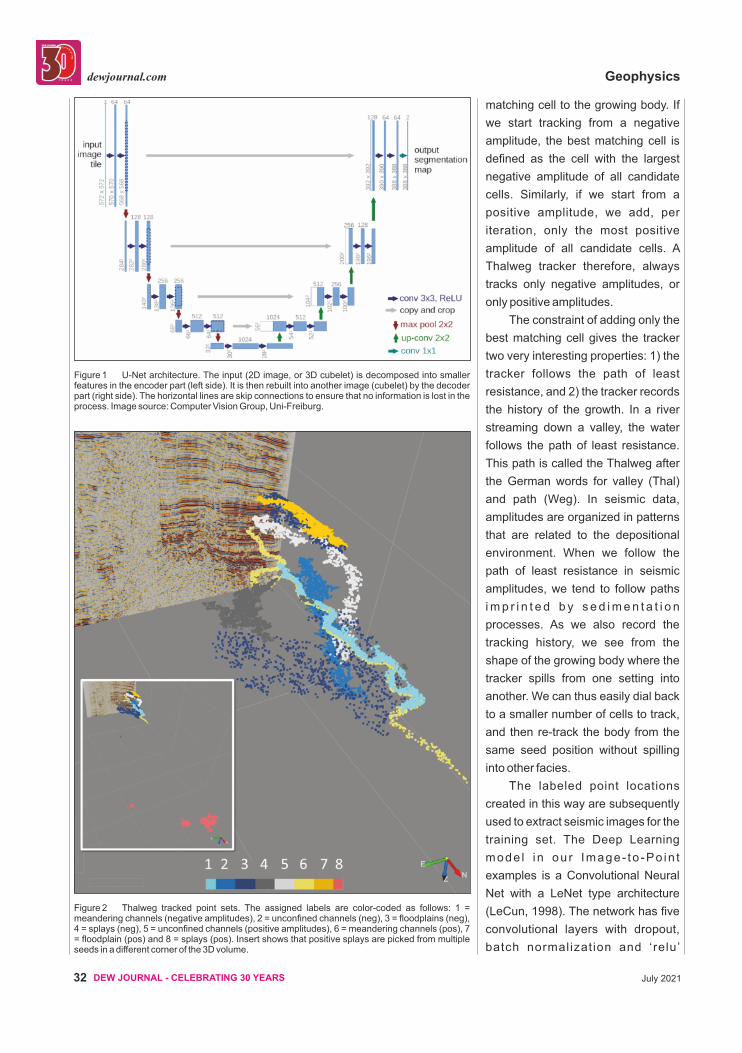
In the Image-to-Image examples
we use a U-Net type of Deep
Learning graph. A U-Net is a
Convolutional type Neural Network
that is known as an auto-encoder
(Ronneberger et.al . , 2015). I t
consists of an encoder part and a
decoder part (Fig. 1). The encoder
decomposes the input image
sequent ia l ly in to smal ler-s ize
features. The decoder recombines
the features sequentially into larger-
size components until the target
image emerges. In other words, a U-
Net transforms an image to another
image of exactly the same size.
U-Nets can be used to solve
s e g m e n t a t i o n p r o b l e m s a n d
regression problems. In the case of
segmentation, the target output is a
binary mask, e.g., an image (cubelet)
with 0’s and 1’s as in our fault imaging
example, or values with 1, 2, …, N, as
in the seismic facies segmentation
example.
IMAGE-TO-POINT EXAMPLES
The first example is from a 3D dataset
covering the Maui Gas Field in the
Taranaki Basin, offshore New
Zealand. Our target is an interval with
stacked meandering channels
deposited during the Miocene. The
channels are easily recognizable on
horizon / time-slices with a Similarity
attribute or with RGB blended
spectral components. Such attribute
displays are helpful when picking
Thalweg tracker seed positions for
the following geomorphological
features: meandering channels,
unconfined channels, floodplains and
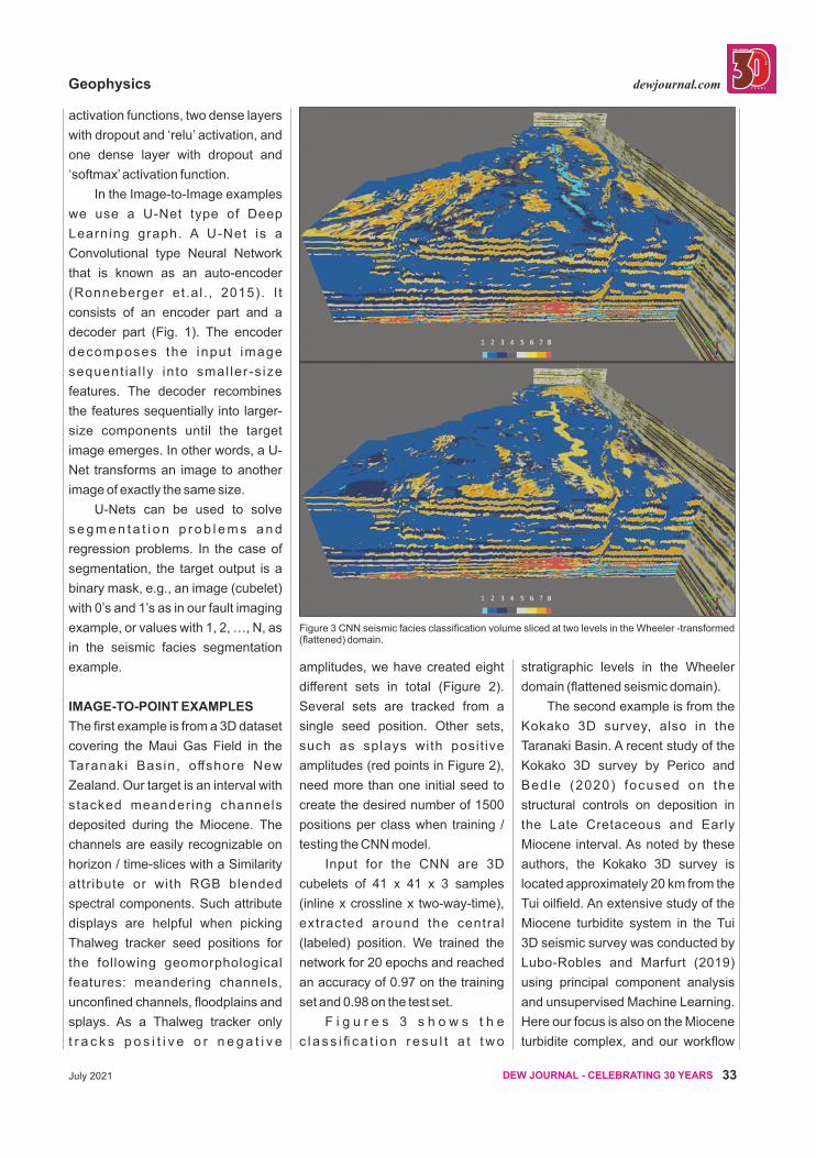
splays. As a Thalweg tracker only
t r a c k s p o s i t i v e o r n e g a t i v e
amplitudes, we have created eight
different sets in total (Figure 2).
Several sets are tracked from a
single seed position. Other sets,
such as splays with posit ive
amplitudes (red points in Figure 2),
need more than one initial seed to
create the desired number of 1500
positions per class when training /
testing the CNN model.
Input for the CNN are 3D
cubelets of 41 x 41 x 3 samples
(inline x crossline x two-way-time),
extracted around the central
(labeled) position. We trained the
network for 20 epochs and reached
an accuracy of 0.97 on the training
set and 0.98 on the test set.
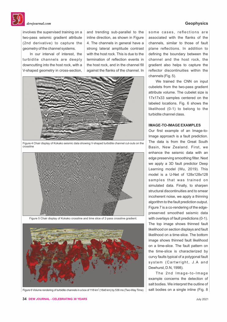
F i g u r e s 3 s h o w s t h e
c l a s s i fi c a t i o n r e s u l t a t t w o
stratigraphic levels in the Wheeler
domain (flattened seismic domain).
The second example is from the
Kokako 3D survey, also in the
Taranaki Basin. A recent study of the
Kokako 3D survey by Perico and
Bedle (2020) focused on the
structural controls on deposition in
the Late Cretaceous and Early
Miocene interval. As noted by these
authors, the Kokako 3D survey is
located approximately 20 km from the
Tui oilfield. An extensive study of the
Miocene turbidite system in the Tui
3D seismic survey was conducted by
Lubo-Robles and Marfurt (2019)
using principal component analysis
and unsupervised Machine Learning.
Here our focus is also on the Miocene
turbidite complex, and our workflow
Figure 1 U-Net architecture. The input (2D image, or 3D cubelet) is decomposed into smaller features in the encoder part (left side). It is then rebuilt into another image (cubelet) by the decoder part (right side). The horizontal lines are skip connections to ensure that no information is lost in the process. Image source: Computer Vision Group, Uni-Freiburg.
Figure 2 Thalweg tracked point sets. The assigned labels are color-coded as follows: 1 = meandering channels (negative amplitudes), 2 = unconfined channels (neg), 3 = floodplains (neg), 4 = splays (neg), 5 = unconfined channels (positive amplitudes), 6 = meandering channels (pos), 7 = floodplain (pos) and 8 = splays (pos). Insert shows that positive splays are picked from multiple seeds in a different corner of the 3D volume.
Figure 3 CNN seismic facies classification volume sliced at two levels in the Wheeler -transformed (flattened) domain.
GeophysicsGeophysics
32 DEW JOURNAL - CELEBRATING 30 YEARS July 2021
dewjournal.com
33DEW JOURNAL - CELEBRATING 30 YEARSJuly 2021
dewjournal.com
matching cell to the growing body. If
we start tracking from a negative
amplitude, the best matching cell is
defined as the cell with the largest
negative amplitude of all candidate
cells. Similarly, if we start from a
positive amplitude, we add, per
iteration, only the most positive
amplitude of all candidate cells. A
Thalweg tracker therefore, always
tracks only negative amplitudes, or
only positive amplitudes.
The constraint of adding only the
best matching cell gives the tracker
two very interesting properties: 1) the
tracker follows the path of least
resistance, and 2) the tracker records
the history of the growth. In a river
streaming down a valley, the water
follows the path of least resistance.
This path is called the Thalweg after
the German words for valley (Thal)
and path (Weg). In seismic data,
amplitudes are organized in patterns
that are related to the depositional
environment. When we follow the
path of least resistance in seismic
amplitudes, we tend to follow paths
i m p r i n t e d b y s e d i m e n t a t i o n
processes. As we also record the
tracking history, we see from the
shape of the growing body where the
tracker spills from one setting into
another. We can thus easily dial back
to a smaller number of cells to track,
and then re-track the body from the
same seed position without spilling
into other facies.
The labeled point locations
created in this way are subsequently
used to extract seismic images for the
training set. The Deep Learning
mode l i n ou r Image- to -Po in t
examples is a Convolutional Neural
Net with a LeNet type architecture
(LeCun, 1998). The network has five
convolutional layers with dropout,
batch normalization and ‘relu’
activation functions, two dense layers
with dropout and ‘relu’ activation, and
one dense layer with dropout and
‘softmax’ activation function.
In the Image-to-Image examples
we use a U-Net type of Deep
Learning graph. A U-Net is a
Convolutional type Neural Network
that is known as an auto-encoder
(Ronneberger et.al . , 2015). I t
consists of an encoder part and a
decoder part (Fig. 1). The encoder
decomposes the input image
sequent ia l ly in to smal ler-s ize
features. The decoder recombines
the features sequentially into larger-
size components until the target
image emerges. In other words, a U-
Net transforms an image to another
image of exactly the same size.
U-Nets can be used to solve
s e g m e n t a t i o n p r o b l e m s a n d
regression problems. In the case of
segmentation, the target output is a
binary mask, e.g., an image (cubelet)
with 0’s and 1’s as in our fault imaging
example, or values with 1, 2, …, N, as
in the seismic facies segmentation
example.
IMAGE-TO-POINT EXAMPLES
The first example is from a 3D dataset
covering the Maui Gas Field in the
Taranaki Basin, offshore New
Zealand. Our target is an interval with
stacked meandering channels
deposited during the Miocene. The
channels are easily recognizable on
horizon / time-slices with a Similarity
attribute or with RGB blended
spectral components. Such attribute
displays are helpful when picking
Thalweg tracker seed positions for
the following geomorphological
features: meandering channels,
unconfined channels, floodplains and
splays. As a Thalweg tracker only
t r a c k s p o s i t i v e o r n e g a t i v e
amplitudes, we have created eight
different sets in total (Figure 2).
Several sets are tracked from a
single seed position. Other sets,
such as splays with posit ive
amplitudes (red points in Figure 2),
need more than one initial seed to
create the desired number of 1500
positions per class when training /
testing the CNN model.
Input for the CNN are 3D
cubelets of 41 x 41 x 3 samples
(inline x crossline x two-way-time),
extracted around the central
(labeled) position. We trained the
network for 20 epochs and reached
an accuracy of 0.97 on the training
set and 0.98 on the test set.
F i g u r e s 3 s h o w s t h e
c l a s s i fi c a t i o n r e s u l t a t t w o
stratigraphic levels in the Wheeler
domain (flattened seismic domain).
The second example is from the
Kokako 3D survey, also in the
Taranaki Basin. A recent study of the
Kokako 3D survey by Perico and
Bedle (2020) focused on the
structural controls on deposition in
the Late Cretaceous and Early
Miocene interval. As noted by these
authors, the Kokako 3D survey is
located approximately 20 km from the
Tui oilfield. An extensive study of the
Miocene turbidite system in the Tui
3D seismic survey was conducted by
Lubo-Robles and Marfurt (2019)
using principal component analysis
and unsupervised Machine Learning.
Here our focus is also on the Miocene
turbidite complex, and our workflow
Figure 1 U-Net architecture. The input (2D image, or 3D cubelet) is decomposed into smaller features in the encoder part (left side). It is then rebuilt into another image (cubelet) by the decoder part (right side). The horizontal lines are skip connections to ensure that no information is lost in the process. Image source: Computer Vision Group, Uni-Freiburg.
Figure 2 Thalweg tracked point sets. The assigned labels are color-coded as follows: 1 = meandering channels (negative amplitudes), 2 = unconfined channels (neg), 3 = floodplains (neg), 4 = splays (neg), 5 = unconfined channels (positive amplitudes), 6 = meandering channels (pos), 7 = floodplain (pos) and 8 = splays (pos). Insert shows that positive splays are picked from multiple seeds in a different corner of the 3D volume.
Figure 3 CNN seismic facies classification volume sliced at two levels in the Wheeler -transformed (flattened) domain.
GeophysicsGeophysics
34 DEW JOURNAL - CELEBRATING 30 YEARS July 2021
dewjournal.com
35DEW JOURNAL - CELEBRATING 30 YEARSJuly 2021
dewjournal.com
involves the supervised training on a
two-pass seismic gradient attribute
(2nd derivative) to capture the
geometry of the channel systems.
In our interval of interest, the
turbidi te channels are deeply
downcutting into the host rock, with a
V-shaped geometry in cross-section,
and trending sub-parallel to the
inline direction, as shown in Figure
4. The channels in general have a
strong lateral amplitude contrast
with the host rock. This is due to the
termination of reflection events in
the host rock, and in the channel fill
against the flanks of the channel. In
s o m e c a s e s , r e fl e c t i o n s a r e
associated with the flanks of the
channels, similar to those of fault
plane reflections. In addition to
defining the boundary between the
channel and the host rock, the
gradient also helps to capture the
reflector discontinuities within the
channels (Fig. 5).
We trained the CNN on input
cubelets from the two-pass gradient
attribute volume. The cubelet size is
17x17x33 samples centered on the
labeled locations. Fig. 6 shows the
likelihood (0-1) to belong to the
turbidite channel class.
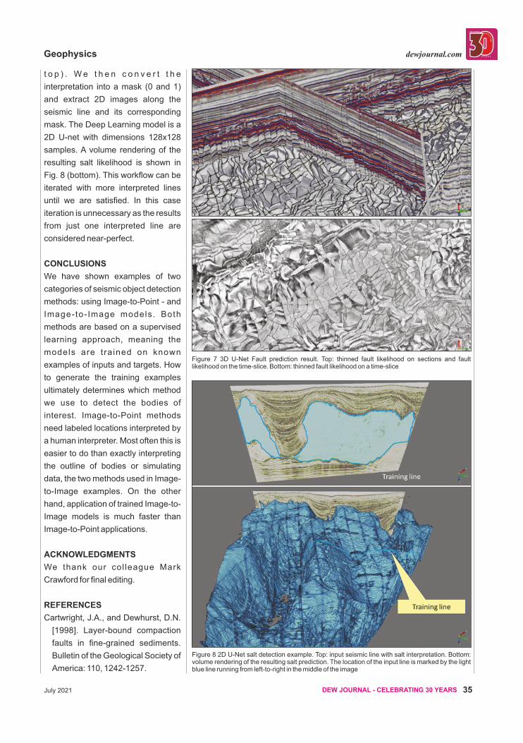
IMAGE-TO-IMAGE EXAMPLES
Our first example of an Image-to-
Image approach is a fault prediction.
The data is from the Great South
Basin, New Zealand. First, we
enhance the seismic data with an
edge preserving smoothing filter. Next
we apply a 3D fault predictor Deep
Learning model (Wu, 2019). This
model is a U-Net of 128x128x128
samples that was t ra ined on
simulated data. Finally, to sharpen
structural discontinuities and to smear
incoherent noise, we apply a thinning
algorithm to the fault prediction output.
Figure 7 is a co-rendering of the edge-
preserved smoothed seismic data
with overlays of fault predictions (0-1).
The top image shows thinned fault
likelihood on section displays and fault
likelihood on a time-slice. The bottom
image shows thinned fault likelihood
on a time-slice. The fault pattern on
the time-slice is characterized by
curvy faults typical of a polygonal fault
sys tem (Car tw r igh t , J .A and
Dewhurst, D.N, 1998).
Th e 2 n d Ima g e - t o - Ima g e
example concerns the detection of
salt bodies. We interpret the outline of
salt bodies on a single inline (Fig. 8 2Figure 6 Volume rendering of turbidite channels in a box of 118 km (18x6 km) by 536 ms (Two-Way Time)
Figure 5 Chair display of Kokako crossline and time slice of 2-pass crossline gradient.
Figure 4 Chair display of Kokako seismic data showing V-shaped turbidite channel cut-outs on the crossline
t o p ) . W e t h e n c o n v e r t t h e
interpretation into a mask (0 and 1)
and extract 2D images along the
seismic line and its corresponding
mask. The Deep Learning model is a
2D U-net with dimensions 128x128
samples. A volume rendering of the
resulting salt likelihood is shown in
Fig. 8 (bottom). This workflow can be
iterated with more interpreted lines
until we are satisfied. In this case
iteration is unnecessary as the results
from just one interpreted line are
considered near-perfect.
CONCLUSIONS
We have shown examples of two
categories of seismic object detection
methods: using Image-to-Point - and
Image-to- Image models. Both
methods are based on a supervised
learning approach, meaning the
models are trained on known
examples of inputs and targets. How
to generate the training examples
ultimately determines which method
we use to detect the bodies of
interest. Image-to-Point methods
need labeled locations interpreted by
a human interpreter. Most often this is
easier to do than exactly interpreting
the outline of bodies or simulating
data, the two methods used in Image-
to-Image examples. On the other
hand, application of trained Image-to-
Image models is much faster than
Image-to-Point applications.
ACKNOWLEDGMENTS
We thank our col league Mark
Crawford for final editing.
REFERENCES
Cartwright, J.A., and Dewhurst, D.N.
[1998]. Layer-bound compaction
faults in fine-grained sediments.
Bulletin of the Geological Society of
America: 110, 1242-1257.
Figure 7 3D U-Net Fault prediction result. Top: thinned fault likelihood on sections and fault likelihood on the time-slice. Bottom: thinned fault likelihood on a time-slice
Figure 8 2D U-Net salt detection example. Top: input seismic line with salt interpretation. Bottom: volume rendering of the resulting salt prediction. The location of the input line is marked by the light blue line running from left-to-right in the middle of the image
GeophysicsGeophysics
34 DEW JOURNAL - CELEBRATING 30 YEARS July 2021
dewjournal.com
35DEW JOURNAL - CELEBRATING 30 YEARSJuly 2021
dewjournal.com
involves the supervised training on a
two-pass seismic gradient attribute
(2nd derivative) to capture the
geometry of the channel systems.
In our interval of interest, the
turbidi te channels are deeply
downcutting into the host rock, with a
V-shaped geometry in cross-section,
and trending sub-parallel to the
inline direction, as shown in Figure
4. The channels in general have a
strong lateral amplitude contrast
with the host rock. This is due to the
termination of reflection events in
the host rock, and in the channel fill
against the flanks of the channel. In
s o m e c a s e s , r e fl e c t i o n s a r e
associated with the flanks of the
channels, similar to those of fault
plane reflections. In addition to
defining the boundary between the
channel and the host rock, the
gradient also helps to capture the
reflector discontinuities within the
channels (Fig. 5).
We trained the CNN on input
cubelets from the two-pass gradient
attribute volume. The cubelet size is
17x17x33 samples centered on the
labeled locations. Fig. 6 shows the
likelihood (0-1) to belong to the
turbidite channel class.
IMAGE-TO-IMAGE EXAMPLES
Our first example of an Image-to-
Image approach is a fault prediction.
The data is from the Great South
Basin, New Zealand. First, we
enhance the seismic data with an
edge preserving smoothing filter. Next
we apply a 3D fault predictor Deep
Learning model (Wu, 2019). This
model is a U-Net of 128x128x128
samples that was t ra ined on
simulated data. Finally, to sharpen
structural discontinuities and to smear
incoherent noise, we apply a thinning
algorithm to the fault prediction output.
Figure 7 is a co-rendering of the edge-
preserved smoothed seismic data
with overlays of fault predictions (0-1).
The top image shows thinned fault
likelihood on section displays and fault
likelihood on a time-slice. The bottom
image shows thinned fault likelihood
on a time-slice. The fault pattern on
the time-slice is characterized by
curvy faults typical of a polygonal fault
sys tem (Car tw r igh t , J .A and
Dewhurst, D.N, 1998).
Th e 2 n d Ima g e - t o - Ima g e
example concerns the detection of
salt bodies. We interpret the outline of
salt bodies on a single inline (Fig. 8 2Figure 6 Volume rendering of turbidite channels in a box of 118 km (18x6 km) by 536 ms (Two-Way Time)
Figure 5 Chair display of Kokako crossline and time slice of 2-pass crossline gradient.
Figure 4 Chair display of Kokako seismic data showing V-shaped turbidite channel cut-outs on the crossline
t o p ) . W e t h e n c o n v e r t t h e
interpretation into a mask (0 and 1)
and extract 2D images along the
seismic line and its corresponding
mask. The Deep Learning model is a
2D U-net with dimensions 128x128
samples. A volume rendering of the
resulting salt likelihood is shown in
Fig. 8 (bottom). This workflow can be
iterated with more interpreted lines
until we are satisfied. In this case
iteration is unnecessary as the results
from just one interpreted line are
considered near-perfect.
CONCLUSIONS
We have shown examples of two
categories of seismic object detection
methods: using Image-to-Point - and
Image-to- Image models. Both
methods are based on a supervised
learning approach, meaning the
models are trained on known
examples of inputs and targets. How
to generate the training examples
ultimately determines which method
we use to detect the bodies of
interest. Image-to-Point methods
need labeled locations interpreted by
a human interpreter. Most often this is
easier to do than exactly interpreting
the outline of bodies or simulating
data, the two methods used in Image-
to-Image examples. On the other
hand, application of trained Image-to-
Image models is much faster than
Image-to-Point applications.
ACKNOWLEDGMENTS
We thank our col league Mark
Crawford for final editing.
REFERENCES
Cartwright, J.A., and Dewhurst, D.N.
[1998]. Layer-bound compaction
faults in fine-grained sediments.
Bulletin of the Geological Society of
America: 110, 1242-1257.
Figure 7 3D U-Net Fault prediction result. Top: thinned fault likelihood on sections and fault likelihood on the time-slice. Bottom: thinned fault likelihood on a time-slice
Figure 8 2D U-Net salt detection example. Top: input seismic line with salt interpretation. Bottom: volume rendering of the resulting salt prediction. The location of the input line is marked by the light blue line running from left-to-right in the middle of the image
GeophysicsGeophysics
36 DEW JOURNAL - CELEBRATING 30 YEARS July 2021
dewjournal.com
LeCun, Y., Bottau, L., Bengio, Y., and
Haffner, P. [1998]. Gradient-based
Learning Applied to Document
Recognition. Proc. of the IEEE,
November 1998.
De Groot, P., Pelissier, M., and van
H o u t , M . [ 2 0 2 1 ] . S e i s m i c
classification: A Thalweg tracking/
ML approach. First Break, Vol. 39,
March 2021, pg. 59-64.
Lubo-Robles, D., and Marfurt, K. J.,
[2019]. Independent component
a n a l y s i s f o r r e s e r v o i r
geomorphology and unsupervised
seismic facies classification in the
Taranaki Basin, New Zealand,
Interpretation, 7:3, SE19-SE42.
Meldahl, P., Heggland, R., De Groot,
P. and Bril, A. [1999]. The chimney
cube, an example o f semi-
automated detection of seismic
objects by directive attributes and
n e u r a l n e t w o r k s : P a r t 1 ;
M e t h o d o l o g y . 6 9 t h S E G
conference, Houston.
Meldahl, P., Heggland, R., De Groot,
P. and Bril, A. [1999]. The chimney
cube, an example o f semi-
automated detection of seismic
objects by directive attributes and
n e u r a l n e t w o r k s : P a r t 2 ;
I n t e r p r e t a t i o n . 6 9 t h S E G
conference, Houston.
Pelissier, M., Singh, R., Qayyum, F.,
de Groot, P., and Romanova, V.
[2016] Guided Voxels for Mapping
Thalweg and Associated Margins.
7 8 t h E A G E C o n f e r e n c e &
Exhibition 2016, Vienna, Austria,
30 May – 2 June 2016.
Perico, E, and Bedle, H., [2020].,
Seismic interpretation of structural
features in the Kokako 3D seismic
a rea , Taranak i Bas in (New
Zealand, SEG Technical Program
Expanded Abstracts 2020, SP
1130-1134.
Ronneberger, O., Fischer, P. and
B r o x , T . , 2 0 1 5 . U - N e t :
Convolutional Networks for
Biomedical Image Segmentation.
Medical Image Computing and
Computer-Assisted Intervention
(MICCAI), Springer, LNCS,
Vol.9351: 234--241, 2015.
Wu, X, Liang, L., Shi, Y. and Fomel,
S. [2019] FaultSeg3D: Using
synthetic data sets to train an end-
to-end convolut ional neura l
network for 3D seismic fault
segmentation. GEOPHYSICS, Vol.
84, No. 3 (May-June 2019); P.
IM35–IM45, 11 FIGS. 10.1190/
GEO2018-0646.1 dewjournal.com
about the authors
Paul de Groot holds M.Sc. (1981) and Ph.D. (1995) degrees in geophysics
from Delft University of Technology. From 1981 to 1990 Paul worked for Shell
in research, seismic processing, quantitative data analysis, seismic
interpretation and E&P software support. From 1991 to 1995 Paul was a
research geophysicist at TNO Institute of Applied Geosciences. In 1995 he
co-founded dGB Earth Sciences, the company behind OpendTect, the
world’s only open source seismic interpretation system. He was the
company’s CEO until 2019 and currently serves as Geoscience Manager.
He is a member of SEG, EAGE, KNGMG and PGK.
Mike Pelissier received a B.Sc. in geophysics from the State University of
New York at Binghamton, an M.Sc. in geophysics from the Colorado School
of Mines, and a Ph.D. in geophysics from the University of London. He joined
the industry in 1979 and has held various positions focused on technology
development, seismic interpretation and reservoir characterization with
Phillips Petroleum Company, Marathon Oil Company, CGG, Roc Oil and
PetroChina. He is Principal QI Geophysicist for GGRE Asia, and an associate
of dGB Earth Sciences and SGS. His interests include the application of
advanced interpretation technologies to both seismic reflection and
diffraction data for field development and reservoir management. Mike is a
member of GSL, EAGE and SEG.
Hesham Refayee earned his master and PhD from Missouri University of
Science and Technology (MS&T), USA in geology and geophysics in 2008,
2012 respectively and his BSc in geology from Tripoli University in 1998. With
+10 years of experience in oil and gas industry, Hesham, a senior geoscientist
with dGB Earth Sciences, specializes in seismic data interpretation; conventional
and unconventional assets, attribute analysis, ML, and petrophysics.
Marieke van Hout- de Groot holds a M.Sc. (2010) from the Behavioral
Science Faculty of the Technical University of Twente, where she mainly
focused on statistical research. Next to this she successfully completed the
course: ‘Geologic Interpretation of seismic data’, which is part of the Master
Petroleum Geophysics at the Technical University of Delft. Marieke started
her career at the geoscience department of TNO, the Dutch Technical
Research Institution, she is now the Executive Vice President of the Asia
Pacific region and the Chief Marketing Officer. Marieke is especially
interested in Machine Learning and Geothermal Energy.
Geophysics