subsurface exploration: engineering geophysics
TRANSCRIPT
Chapter 4
Subsurface exploration: engineering geophysics
INTRODUCTION The most widespread site investigation techniques, such as those described in Chapters 5, 7, 8 and 9, involve the drilling of holes in the ground, sampling at discrete points, and in situ or laboratory testing. Given the relatively small sums of money involved in ground investigations of this type, only a very small proportion of the volume of soil and rock that will affect construction can be sampled and tested. Geophysical techniques offer the chance to overcome some of the problems inherent in more conventional ground investigation techniques. Many methods exist with the potential of providing profiles and sections, so that (for example) the ground between boreholes can be checked to see whether ground conditions at the boreholes are representative of those elsewhere. Geophysical techniques also exist which can be of help in locating cavities, backfilled mineshafts, and dissolution features in carbonate rocks, and there are other techniques which can be extremely useful in determining the stiffness properties of the ground. Yet, at the time of writing, geophysics is only rarely used in ground investigations. Various reasons have been put forward to explain this fact, including:
1. poor planning of geophysical surveys (see Chapter 1), by engineers ignorant of the techniques; and
2. overoptimism by geophysicists, leading to a poor reputation for the available techniques.
Most geophysics carried out during ground investigations is controlled by geologists or physicists. Generally, their educational background is either a geology or physics first degree, with a Masters postgraduate degree in geophysics. Such people often have considerable expertise in the geophysical techniques they offer, but they have very little idea of the contractual constraints within which civil and construction engineers must work. The writers’ view is that an understanding of geophysics is not beyond the capabilities of most civil engineers, who generally have a good education in physics. This chapter therefore provides an engineer’s view of engineering geophysics. It does not provide the conventional views of engineering geophysics, but deliberately concentrates on identifying those situations where geophysical techniques are likely to be of most help to engineers.
Engineering needs Most geophysical techniques have as their origin the oil and mining industries. In such industries the primary need of a developer is to identify the locations of minerals for exploitation, against a background of relatively large financial rewards once such deposits are found. Geophysics plays a vital role intermediate between geological interpretation of the ground and its structure, and the drilling of exploratory holes to confirm the presence of ores, oil or gas. In most cases the minerals are deep, and drilling is very expensive — geophysics
Site Investigation
2
allows optimization of the drilling investigation, amongst other things. Many mineral explorations will be centred upon deep deposits, where ground conditions are spatially relatively uniform, and geological structures are large. Geophysical techniques are relatively cheap, and are highly regarded in such a speculative environment, even though they may not always be successful. In contrast, ground investigations are carried out against a professional, contractual and legal background which often demands relatively fine resolution and certainty of result. The idea that a test or method will be successful and yield useful data only in a proportion of the cases in which it is used is unacceptable. As was noted in Chapter 1, it is necessary for a geotechnical engineer to weigh carefully the need for each element of his ground investigation. He will often have to persuade his client to provide additional funds for non-standard techniques, and if these are unsuccessful the client may not be convinced of his competence. Therefore, when using geophysical techniques during ground investigation, as part of the engineering design process, great care is needed. The engineer should convince himself of the need for such a survey, and should take care of ensure that only appropriate and properly designed surveys are carried out. Unfortunately, there has been a widespread failure of geophysical techniques to perform as expected during ground investigations. So far as geophysical methods of subsoil exploration are concerned, there can be no doubt about their desirability and merits, because they are extremely cheap: they are even cheaper than geologists. They have only one disadvantage, and that is we never know in advance whether they are going to work or not! During my professional career, I have been intimately connected with seven geophysical surveys. In every case the physicists in charge of the exploration anticipated and promised satisfactory results. Yet only the first one was a success; the six others were rather dismal failures.
Terzaghi, 1957 More recently, the view has emerged that it is the planning of the surveys which has been at fault, and that if proper geological advice is sought then all will be well. Too often in the past geophysical methods have been used without due reference to the geological situation, and consequently the results have been disappointing. These failures always appear to be blamed on the method rather than on the misapplication of the method, and this is why many engineers mistrust geophysical methods. The solution to this difficulty is to take better geological advice during the planning of the investigation, and to maintain close geological supervision during its execution.
Burton, 1975
It is our belief that both of these attitudes are over-simplistic. Whilst it is true that most professionals will be overoptimistic in their attempts to gain work, experience of the application of certain techniques during ground investigation is now sufficient to give guidance on techniques which will have a much better than one in seven chance of success. On the other hand, there is a growing trend for geophysical techniques to be integrated into ground investigations in a way which is difficult for a geophysicist to understand — the geophysicist cannot readily appreciate the engineer’s priorities and requirements, and may not be sufficiently familiar with the science of soil mechanics. In summary, the majority of problems arise because of:
1. the expectations of engineers that all techniques will be 100% successful;
Subsurface Exploration: Engineering Geophysics
3
2. poor inter-disciplinary understanding between engineers, engineering geologists and geophysicists;
3. a lack of communication, particularly with respect to the objectives of ground investigation;
4. a lack of objective appraisal of the previous success of geophysical techniques in the particular geological setting, given the objectives of the survey;
5. poor planning of the execution of the survey; and 6. the use of inappropriate science (for example, measurements of compressional wave
velocities).
It is important to be clear as to the reason for using geophysics in ground investigations. In practice there are at least five different functions which can be fulfilled. The variability of natural near-surface ground has already been noted, as has the limited finance available to make boreholes. Geophysical techniques can contribute very greatly to the process of ground investigation by allowing an assessment, in qualitative terms, of the lateral variability of the near-surface materials beneath a site. Non-contacting techniques such as ground conductivity, magnetometry, and gravity surveying are very useful, as are some surface techniques (for example, electrical resistivity traversing). Geophysical techniques can also be used for vertical profiling. Here the objective is to determine the junctions between the different beds of soil or rock, in order either to correlate among boreholes or to infill between them. Techniques used for this purpose include electrical resistivity depth profiling, seismic methods, the surface wave technique, and geophysical borehole logging. Some are surface techniques, but the majority are carried out down-hole. Sectioning is carried out to provide cross-sections of the ground, generally to give details of beds and layers. It is potentially useful when there are marked contrasts in the properties of the ground (as between the stiffness and strength of clay and rock), and the investigation is targeted at finding the position of a geometrically complex interface, or when there is a need to find hard inclusions or cavities. In addition, as with vertical profiling, these techniques can allow extrapolation of borehole data to areas of the site which have not been the subject of borehole investigation. Examples of such techniques are seismic tomography, ground probing radar, and seismic reflection. One of the major needs of any ground investigation is the classification of the subsoil into groups with similar geotechnical characteristics. Geophysical techniques are not generally of great use in this respect, except in limited circumstances. An example occurs where there is a need to distinguish between cohesive and noncohesive soils. Provided that the salinity of the groundwater is low, it is normally possible to distinguish between these two groups of materials using either electrical resistivity or ground conductivity. Finally, almost all geotechnical ground investigations aim to determine stiffness, strength, and other parameters in order to allow design calculations to be carried out. Traditionally, geotechnical engineers felt that the determination of geotechnical parameters from geophysical tests was impossible. The acceptance, within the last decade or so, that the small strain stiffnesses relevant to the design of civil engineering and building works may, in many circumstances be quite similar to the very small strain stiffness (Go or Gmax) that can be determined from seismic methods has led to a worldwide reawakening of interest in this type of method. In selecting a particular geophysical technique for use on a given site, it is essential that the following questions are asked.
Site Investigation
4
1. What is the objective of the survey? It is generally true that users of geophysics expect the survey to provide a number of types of information. In fact, the converse is true. The survey should normally be designed to provide information on a single aspect of the site. A number of examples are given below:
• depth to rockhead; • position of old mineshafts; • corrosivity of the ground; • very small strain stiffness of the ground; • extent of saline intrusion of groundwater; • position of cohesive and granular deposits along a pipeline route.
2. What is the physical property to be measured? Given the ‘target’ of the geophysical investigation, the physical property that is to be measured may be obvious. For example, if the target is to be the determination of the very small strain stiffness of the ground, then it follows that the property that must be measured is the seismic shear wave velocity. But in many cases the success of a geophysical survey will depend upon the choice of the best geophysical method, and the best geophysical method is likely to be the one which is most sensitive to the variations in the ground properties associated with the target. For example, in trying to locate a mineshaft it might be relevant to consider whether metallic debris (for example, winding gear) has been left at the location (making magnetic methods likely to be successful) or whether the shaft is empty and relatively close to the ground (making gravity methods attractive).
3. Which method is most suited to the geometry of the target?
Geophysical targets range from cavities to boundaries between rock types, and from measurements of stiffness to the location of geological marker beds. The particular geometry of the target may make one particular technique very favourable (for example, the determination of the position of rockhead (i.e. the junction between rock and the overlying soil) or gassy sediments beneath the sea is often carried out using seismic reflection techniques.
4. Is there previous published experience of the use of this method for this purpose?
Unfortunately it is unusual for engineers and geophysicists to publish their failures, so that the reporting of the successful use of a particular technique for a given target cannot be taken as a guarantee that it will work in a given situation. Conversely, however, the lack of evidence of success in the past should act as a warning. In assessing the likely success of a geophysical method, it will be helpful to consult as widely as possible with specialists and academic researchers.
Some geophysical methods have a very high rate of success, provided that the work is carried out by experienced personnel. Others will have very little chance of success, however well the work is executed.
5. Is the site ‘noisy’? Geophysical methods require the acquisition of data in the field, and that data may be overwhelmed by the presence of interference. The interference will be specific to the chosen geophysical method; seismic surveys may be rendered impractical by the ground-borne noise from nearby roads, or from construction plant; resistivity and conductivity surveys may be interfered with by electrical cables, and gravity surveys will need to be corrected for the effects of nearby buildings, known basements, and embankments.
Subsurface Exploration: Engineering Geophysics
5
6. Are there any records of the ground conditions available? If borehole or other records are available then two approaches are possible. The information can be used to refine the interpretation of the geophysical output, or the geophysical method can be tested blind. The latter method is really only suitable in instances where the geophysical method is claimed to work with great certainty, for example when testing a contractor’s ability to detect voids. In most cases geophysicists will require a reasonable knowledge of the ground conditions in order to optimize the geophysical test method, and the withholding of available data will only jeopardize the success of a survey.
7. Is the sub-soil geometry sufficiently simple to allow interpretation? Some methods of interpretation rely on there being a relatively simple sub-soil geometry, and one which is sufficiently similar to simple physical models used in forward modelling, to provide ‘master curves’. Most models will assume that there is no out-of-plane variability, and that the ground is layered, with each layer being isotropic and homogeneous. Complex three-dimensional structure cannot be interpreted.
8. Is the target too small or too deep to be detected? 9. Is it necessary to use more than one geophysical method for a given site?
Classification of geophysical techniques There are many geophysical techniques available during ground investigation. In this section we attempt to classify them in different ways, to allow the reader to develop a framework within which to select the most appropriate technique(s) for his job. Geophysical techniques may be categorized by the following: Control of input Geophysical methods may be divided into two groups.
1. Passive techniques. The anomalies measured by the technique pre-exist. They cannot be varied by the investigator. Repeat surveys can be carried out to investigate the effects of variations of background ‘noise’, but apart from varying the time of the survey, and the equipment used, no refinement is possible. In using passive techniques, the choice of the precise technique and the equipment to be used are very important. Generally these techniques involve measurements of local variations in the Earth’s natural force fields (for example, gravity and magnetic fields).
2. Active techniques. These techniques measure perturbations created by an input, such
as seismic energy or nuclear radiation. Signal-to-noise ratio can be improved by adding together the results of several surveys (stacking), or by altering the input geometry.
In general, interpretation is more positive for active than for passive techniques, but the cost of active techniques tends to be greater than for passive techniques. Types of measurement Some geophysical techniques detect the spatial difference in the properties of the ground. Such differences (for example, the difference between the density of the ground and that of a water-filled cavity) lead to perturbations of the background level of a particular measurement
Site Investigation
6
(in this case, gravitational pull) which are measured, and must then be interpreted. These perturbations are termed ‘anomalies’. Other geophysical techniques measure particular events (for example, seismic shear wave arrivals, as a function of time), and during interpretation these measurements are converted into properties (in this case, seismic shear wave velocity). A particular geophysical technique will make measurements of only a single type. Techniques that are commonly available measure:
• seismic wave amplitude, as a function of time; • electrical resistivity or conductivity; • electromagnetic radiation; • radioactive radiation; • magnetic flux density; and • gravitational pull.
From a geotechnical point of view, passive techniques require relatively little explanation. The apparatus associated with them can often be regarded as ‘black boxes’. It is sufficient, for example, to note that:
1. gravity methods respond to differences in the mass of their surroundings, which results either from contrasts in the density of the ground, or from variations in geometry (cavities and voids, embankments, hills, etc.);
2. magnetic methods detect differences in the Earth’s magnetic field, which are produced locally by the degree of the magnetic susceptibility (the degree to which a body can be magnetized) of the surroundings. Such methods will primarily detect the differences in the iron content of the ground, whether natural or artificial;
3. Natural gamma logging detects the very small background radiation emitted by certain layers in the ground.
Active methods require more consideration, because surveys using these methods can often be optimized if the principles of the methods are understood. The seismic method is rapidly becoming more popular in geotechnical investigations because of its ability to give valuable information on the stiffness variations in the ground. The seismic method relies on the differences in velocity of elastic or seismic waves through different geological or man-made materials. An elastic wave is generated in the ground by impactive force (a falling weight or hammer blow) or explosive charge. The resulting ground motion is detected at the surface by vibration detectors (geophones). Measurements of time intervals between the generation of the wave and its reception at the geophones enable the velocity of the elastic wave through different media in the ground to be determined. A seismic disturbance in elastically homogenous ground, whether natural or artificially induced, will cause the propagation of four types of elastic wave, which travel at different velocities. These waves are as follows.
1. Longitudinal waves (‘P’ waves). These are propagated as spherical fronts from the source of the seismic disturbance. The motion of the ground is in the direction of propagation. These waves travel faster than any other type of wave generated by the seismic disturbance.
2. Transverse or shear waves (‘S’ waves). Transverse waves, like longitudinal waves, are propagated as spherical fronts. The ground motion, however, is perpendicular to the direction of propagation in this case. S waves have two degrees of freedom unlike P waves which only have one. In practice, the S wave motion is resolved into
Subsurface Exploration: Engineering Geophysics
7
components parallel and perpendicular to the surface of the ground, which are known respectively as SH and SV waves. The maximum velocity of an S wave is about 70% of the P wave velocity through the same medium.
3. Rayleigh waves. These waves travel only along the ground surface. The particle motion associated with these waves is elliptical (in the vertical plane). Rayleigh waves generally attenuate rapidly with distance. The velocity of these waves depends on wavelength and the thickness of the surface layer. In general, Rayleigh waves travel slower than P or S waves.
4. Love waves. These are surface waves which occur only when the surface layer has a low P wave velocity with respect to the underlying layer. The wave motion is horizontal and transverse. The velocity of these waves may be equal to the S wave velocity of the surface layer or the underlying layer depending on the wavelength of the Love wave. Energy sources used in seismic work do not generate Love waves to a significant degree. Love waves are therefore generally considered unimportant in seismic investigation.
Soils generally comprise two phases (the soil skeleton and its interstitial water) and may have three phases (soil, water and air). P-wave energy travels through both the skeleton and the pore fluid, whilst S-wave energy travels only through the skeleton, because the pore fluid has no shear resistance. Traditionally, the geophysical industry has made almost exclusive use of P waves. These are easy to detect, since they are the first arrivals on the seismic record. However, in relative soft saturated near-surface sediments, such as are typically encountered in the temperate regions of the world, the P-wave velocity is dominated by the bulk modulus of the pore fluid. If the ground is saturated, and the skeleton relatively compressible (i.e. B = 1 (Skempton 1954)), the P-wave velocity will not be much different from that of water (about 1500 m/s). Therefore it is not possible to distinguish between different types of ground on the basis of P-wave velocities until the bulk modulus of the skeleton of the soil or rock is substantially greater than that of water. This is only the case for relatively unweathered and unfractured rocks, for which the P-wave velocity may rise to as much as 7000 m/s. Shear wave energy travels at a speed which is determined primarily by the shear modulus of the soil or rock skeleton, modified by its state of fracturing:
���
����
�=
ρ�
GVs (4.1)
where V, = shear wave velocity, G0 = shear modulus at very small strain and P = bulk density. Since the bulk density of soil is not very variable, typically ranging from 1.6 Mg/rn3 for a soft soil to 3.0Mg/rn3 for a dense rock, the variation of S-wave velocity gives a good guide to the very small strain stiffness variations of the ground. Further, the last decade has brought a realization that (except at very small strain levels) soil does not behave in a linear-elastic manner, and that the strains around engineering works are typically very small. Thus it is now realized that stiffnesses obtained from geophysical methods may be acceptably close to those required for design. For rocks the operational stiffness may be very similar to that obtained from field geophysics, while for soils it is likely to be of the order of two or three times lower. Given the uncertainties of many methods available for determining ground stiffnesses, seismic geophysical methods of determining S-wave velocities are becoming increasingly important in geotechnical site investigations.
Site Investigation
8
Whereas the determination of seismic shear wave velocity has gained increased prominence in site investigations, the use of seismic methods to determine the geometry of the sub-soil appears to have undergone a general decline. This is probably associated with a low level of success of these techniques in shallow investigations. The propagation of seismic waves through near-surface deposits is extremely complex. The particulate, layered and fractured nature of the ground means that waves undergo not only reflection and refraction but also diffraction, thus making modelling of seismic energy transmission impractical. Anisotropy, and complex and gradational soil boundaries often make interpretation impossible. Electrical resistivity and conductivity methods rely on measuring subsurface variations of electrical current flow which are manifest by an increase or decrease in electrical potential between two electrodes. This is represented in terms of electrical resistivity which may be related to changes in rock or soil types. The electrical resistivity methods is commonly used therefore to map lateral and vertical changes in geological (or man-made) materials. The method may also used to:
1. assess the quality of rock/soil masses in engineering terms; 2. determine the depth to the water table (normally in arid or semi-arid areas); 3. map the saline/fresh water interface in coastal regions; 4. locate economic deposits of sand and gravel; and 5. locate buried features such as cavities, pipelines, clay-filled sink holes and buried
channels. The electrical resistivity of a material is defined as the resistance offered by a unit cube of that material to the flow of electrical current between two opposite faces. Most common rock-forming minerals are insulators, with the exception of metalliferous minerals which are usually good conductors. In general, therefore, rocks and soils conduct electricity by electrolytic conduction within the water contained in their pores, fissures, or joints. It follows that the conductivity of rocks and soils is largely dependent upon the amount of water present, the conductivity of the water, and the manner in which the water is distributed within the material (i.e., the porosity, degree of saturation, degree of cementation, and fracture state). These factors are related by Archie’s empirical equation (Archie 1942):
lmw snaρρ = (4.2)
where � = resistivity of the rock or soil, �w = resistivity of the pore water, n = porosity, s degree of saturation, 1=2, m = 1.3-2.5, and a = 0.5-2.5. The manner in which the water is distributed in the rock determines the factor m (cementation factor) which for loose (uncemented sands) is about 1.3 (Van Zijl 1978). The validity of Archie’s equation is, however, dependent on various factors such as the presence or absence of clay minerals (Griffiths 1946). Guyod (1964) gives a simplified version of Archie’s equation:
2nwρρ = (4.3)
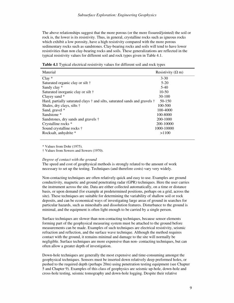
where � = resistivity of the rock/soil, �w = resistivity of the pore water, and n = porosity. Because the conduction of electrical current through the pore water is essentially electrolytic, the conductivity of the pore water must be related to the amount and type of electrolyte within it. Figure 4.1 shows the relation between the salinity of the pore water and the measured resistivity for materials with different porosities. As the salinity of the pore water increases, there is a significant decrease in measured resistivity.
Subsurface Exploration: Engineering Geophysics
9
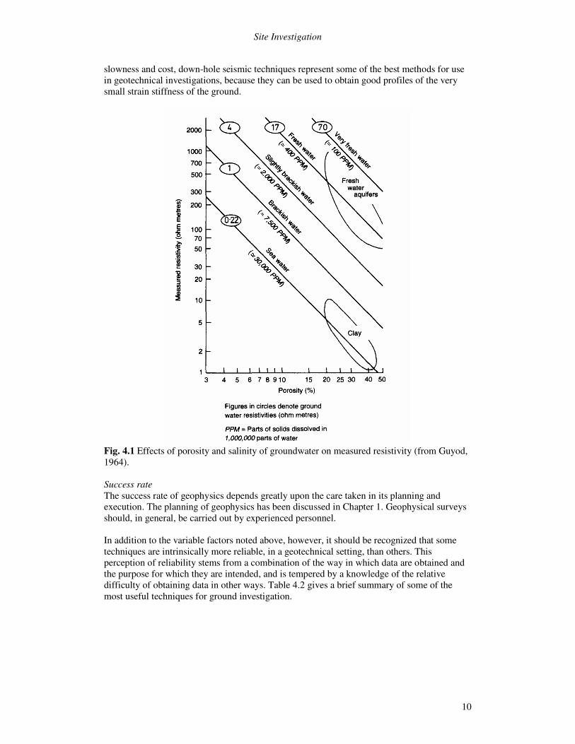
The above relationships suggest that the more porous (or the more fissured/jointed) the soil or rock is, the lower is its resistivity. Thus, in general, crystalline rocks such as igneous rocks which exhibit a low porosity, have a high resistivity compared with the more porous sedimentary rocks such as sandstones. Clay-bearing rocks and soils will tend to have lower resistivities than non clay-bearing rocks and soils. These generalizations are reflected in the typical resistivity values for different soil and rock types given in Table 4.1. Table 4.1 Typical electrical resistivity values for different soil and rock types
* Values from Dohr (1975). † Values from Sowers and Sowers (1970). Degree of contact with the ground The speed and cost of geophysical methods is strongly related to the amount of work necessary to set up the testing. Techniques (and therefore costs) vary very widely. Non-contacting techniques are often relatively quick and easy to use. Examples are ground conductivity, magnetic and ground penetrating radar (GPR) techniques. Here the user carries the instrument across the site. Data are either collected automatically, on a time or distance basis, or upon demand (for example at predetermined positions, perhaps on a grid, across the site). These techniques are suitable for determining the variability of shallow soil or rock deposits, and can be economical ways of investigating large areas of ground in searches for particular hazards, such as mineshafts and dissolution features. Disturbance to the ground is minimal, and the equipment is often light enough to be carried by a single person. Surface techniques are slower than non-contacting techniques, because sensor elements forming part of the geophysical measuring system must be attached to the ground before measurements can be made. Examples of such techniques are electrical resistivity, seismic refraction and reflection, and the surface wave technique. Although the method requires contact with the ground, it remains minimal and damage to the site will normally be negligible. Surface techniques are more expensive than non- contacting techniques, but can often allow a greater depth of investigation. Down-hole techniques are generally the most expensive and time-consuming amongst the geophysical techniques. Sensors must be inserted down relatively deep preformed holes, or pushed to the required depth (perhaps 20m) using penetration testing equipment (see Chapter 5 and Chapter 9). Examples of this class of geophysics are seismic up-hole, down-hole and cross-hole testing, seismic tomography and down-hole logging. Despite their relative
Material Resistivity (� m) Clay * 3-30 Saturated organic clay or silt † 5-20 Sandy clay * 5-40 Saturated inorganic clay or silt † 10-50 Clayey sand * 30-100 Hard, partially saturated clays † and silts, saturated sands and gravels † 50-150 Shales, dry clays, silts † 100-500 Sand, gravel * 100-4000 Sandstone * 100-8000 Sandstones, dry sands and gravels † 200-1000 Crystalline rocks * 200-10000 Sound crystalline rocks † 1000-10000 Rocksalt, anhydrite * >1100
Site Investigation
10
slowness and cost, down-hole seismic techniques represent some of the best methods for use in geotechnical investigations, because they can be used to obtain good profiles of the very small strain stiffness of the ground.
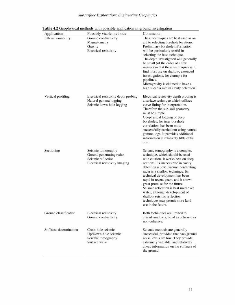
Fig. 4.1 Effects of porosity and salinity of groundwater on measured resistivity (from Guyod, 1964). Success rate The success rate of geophysics depends greatly upon the care taken in its planning and execution. The planning of geophysics has been discussed in Chapter 1. Geophysical surveys should, in general, be carried out by experienced personnel. In addition to the variable factors noted above, however, it should be recognized that some techniques are intrinsically more reliable, in a geotechnical setting, than others. This perception of reliability stems from a combination of the way in which data are obtained and the purpose for which they are intended, and is tempered by a knowledge of the relative difficulty of obtaining data in other ways. Table 4.2 gives a brief summary of some of the most useful techniques for ground investigation.
Subsurface Exploration: Engineering Geophysics
11
Table 4.2 Geophysical methods with possible application in ground investigation Application Possibly viable methods Comments Lateral variability Ground conductivity
Magnetometry Gravity Electrical resistivity
These techniques are best used as an aid to selecting borehole locations. Preliminary borehole information will be particularly useful in selecting the best technique. The depth investigated will generally be small (of the order of a few metres) so that these techniques will find most use on shallow, extended investigations, for example for pipelines. Microgravity is claimed to have a high success rate in cavity detection.
Vertical profiling Electrical resistivity depth probing Natural gamma logging Seismic down-hole logging
Electrical resistivity depth probing is a surface technique which utilizes curve fitting for interpretation. Therefore the sub-soil geometry must be simple. Geophysical logging of deep boreholes, for inter-borehole correlation, has been most successfully carried out using natural gamma logs. It provides additional information at relatively little extra cost.
Sectioning Seismic tomography Ground penetrating radar Seismic reflection Electrical resistivity imaging
Seismic tomography is a complex technique, which should be used with caution. It works best on deep sections. Its success rate in cavity detection is low. Ground penetrating radar is a shallow technique. Its technical development has been rapid in recent years, and it shows great promise for the future. Seismic reflection is best used over water, although development of shallow seismic reflection techniques may permit more land use in the future.
Ground classification Electrical resistivity Ground conductivity
Both techniques are limited to classifying the ground as cohesive or non-cohesive.
Stiffness determination Cross-hole seismic Up/Down-hole seismic Seismic tomography Surface wave
Seismic methods are generally successful, provided that background noise levels are low. They provide extremely valuable, and relatively cheap information on the stiffness of the ground.
Site Investigation
12
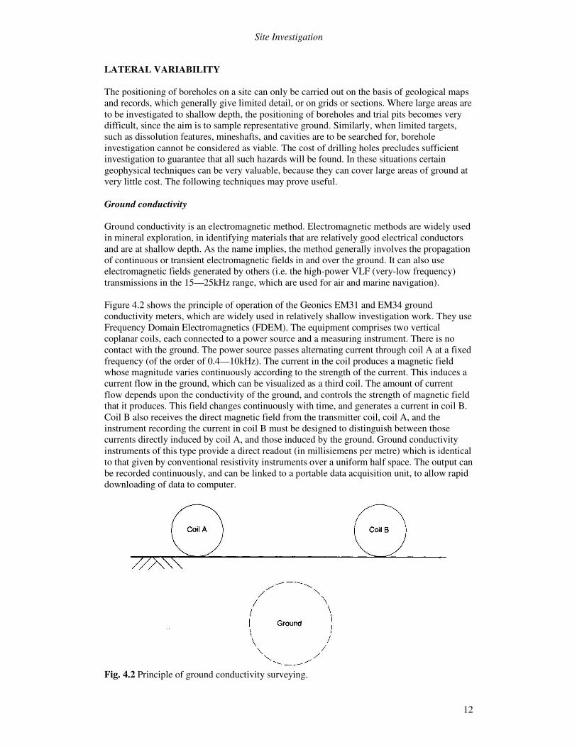
LATERAL VARIABILITY The positioning of boreholes on a site can only be carried out on the basis of geological maps and records, which generally give limited detail, or on grids or sections. Where large areas are to be investigated to shallow depth, the positioning of boreholes and trial pits becomes very difficult, since the aim is to sample representative ground. Similarly, when limited targets, such as dissolution features, mineshafts, and cavities are to be searched for, borehole investigation cannot be considered as viable. The cost of drilling holes precludes sufficient investigation to guarantee that all such hazards will be found. In these situations certain geophysical techniques can be very valuable, because they can cover large areas of ground at very little cost. The following techniques may prove useful. Ground conductivity Ground conductivity is an electromagnetic method. Electromagnetic methods are widely used in mineral exploration, in identifying materials that are relatively good electrical conductors and are at shallow depth. As the name implies, the method generally involves the propagation of continuous or transient electromagnetic fields in and over the ground. It can also use electromagnetic fields generated by others (i.e. the high-power VLF (very-low frequency) transmissions in the 15—25kHz range, which are used for air and marine navigation). Figure 4.2 shows the principle of operation of the Geonics EM31 and EM34 ground conductivity meters, which are widely used in relatively shallow investigation work. They use Frequency Domain Electromagnetics (FDEM). The equipment comprises two vertical coplanar coils, each connected to a power source and a measuring instrument. There is no contact with the ground. The power source passes alternating current through coil A at a fixed frequency (of the order of 0.4—10kHz). The current in the coil produces a magnetic field whose magnitude varies continuously according to the strength of the current. This induces a current flow in the ground, which can be visualized as a third coil. The amount of current flow depends upon the conductivity of the ground, and controls the strength of magnetic field that it produces. This field changes continuously with time, and generates a current in coil B. Coil B also receives the direct magnetic field from the transmitter coil, coil A, and the instrument recording the current in coil B must be designed to distinguish between those currents directly induced by coil A, and those induced by the ground. Ground conductivity instruments of this type provide a direct readout (in millisiemens per metre) which is identical to that given by conventional resistivity instruments over a uniform half space. The output can be recorded continuously, and can be linked to a portable data acquisition unit, to allow rapid downloading of data to computer.
Fig. 4.2 Principle of ground conductivity surveying.
Subsurface Exploration: Engineering Geophysics
13
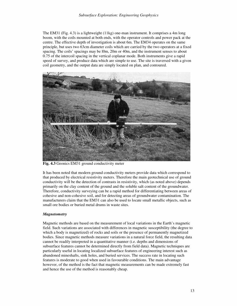
The EM31 (Fig. 4.3) is a lightweight (11kg) one-man instrument. It comprises a 4m long boom, with the coils mounted at both ends, with the operator controls and power pack at the centre. The effective depth of investigation is about 6m. The EM34 operates on the same principle, but uses two 63cm diameter coils which are carried by the two operators at a fixed spacing. The coils’ spacings may be l0m, 20m or 40m, and the instrument senses to about 0.75 of the intercoil spacing in the vertical coplanar mode. Both instruments give a rapid speed of survey, and produce data which are simple to use. The site is traversed with a given coil geometry, and the output data are simply located on plan, and contoured.
Fig. 4.3 Geonics EM31 ground conductivity meter It has been noted that modern ground conductivity meters provide data which correspond to that produced by electrical resistivity meters. Therefore the main geotechnical use of ground conductivity will be the detection of contrasts in resistivity, which (as noted above) depends primarily on the clay content of the ground and the soluble salt content of the groundwater. Therefore, conductivity surveying can be a rapid method for differentiating between areas of cohesive and non-cohesive soil, and for detecting areas of groundwater contamination. The manufacturers claim that the EM31 can also be used to locate small metallic objects, such as small ore bodies or buried metal drums in waste sites. Magnetometry Magnetic methods are based on the measurement of local variations in the Earth’s magnetic field. Such variations are associated with differences in magnetic susceptibility (the degree to which a body is magnetized) of rocks and soils or the presence of permanently magnetized bodies. Since magnetic methods measure variations in a natural force field, the resulting data cannot be readily interpreted in a quantitative manner (i.e. depths and dimensions of subsurface features cannot be determined directly from field data). Magnetic techniques are particularly useful in locating localized subsurface features of engineering interest such as abandoned mineshafts, sink holes, and buried services. The success rate in locating such features is moderate to good when used in favourable conditions. The main advantage however, of the method is the fact that magnetic measurements can be made extremely fast and hence the use of the method is reasonably cheap.
Site Investigation
14
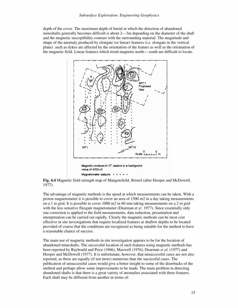
The measurements made in magnetic surveying may be of the vertical component of the Earth’s magnetic field or of the Earth’s total magnetic field strength. Measurements of the vertical component of the Earth’s magnetic field are made mechanically using magnetic balances. The total field strength is measured using fluxgate or proton instruments. For most engineering investigations the proton precession magnetometer is used. Extremely fast magnetic measurements can be made (usually less than 30s are spent at each station) using this instrument because it employs a remote sensing head which requires no levelling. The proton magnetometer is accurate to ± 1 nT1, compared with ±5 nT for the fluxgate instrument. The strength of the Earth’s magnetic field varies between 47000 nT to about 49000 nT from south to north across the British Isles. Observations are normally made on a grid. The station interval along each traverse line forming the grid should not exceed the expected dimensions of the feature to be located. A station interval of between 1 and 2m is normally used for the location of abandoned mineshafts. For the location of clay filled sink holes in chalk McDowell (1975) suggests a station interval (and distance between traverses) of less than half the expected lateral extent of the feature. The field data must be corrected for diurnal and secular variations in the Earth’s magnetic field. Diurnal variation is measured throughout the survey by periodically returning to a base station and measuring the field strength. The field data once corrected for these variations are normally presented in the form of a contoured magnetic map. Figure 4.4 shows a magnetic map for a site at Mangotsfield, Bristol. The contour values are relative to the regional magnetic field strength. Characteristic shapes may be recognized from magnetic maps and related to subsurface bodies in terms of general geometry and orientation (if they are not equidimensional) magnetic profiles are often drawn across anomalies to aid interpretation. Interpretation of magnetic data is qualitative. Detailed analysis of the data may be carried out by comparing field data with theoretical anomalies produced by physical models. These models are altered to produce a best fit with the field data. The field data, however, can be highly ambiguous and a unique relationship between the anomalies produced by a single physical model and the field prototype rarely exists. In some cases the depth of a subsurface feature may be estimated from the width of the anomaly produced. Measured field strengths are seriously affected by interference from electrical cables, electric railways, moving vehicles and highly heterogeneous ground. The latter is a common feature of urban areas in which the abundance of old foundations, buried services, and waste material gives rise to complex anomalies which can easily mask anomalies produced by singular features of engineering interest. Ideal sites for the use of magnetic methods are on open little-developed land, free from extraneous interference. The method may be used successfully in developed areas, but care should be taken in choosing the magnetic method. Moreover, the engineering geophysicist should be presented with all the available data concerning the history of the site, which may have been obtained during the preliminary desk study. The magnitude of magnetic anomalies associated with localized features will depend on the depth of the feature and the height of the sensor above the ground. A sensor height of 1 m above ground level has proved convenient and adequately free from magnetic variations of the top soil (Hooper and McDowell 1977). In general, the magnetic anomaly produced by a subsurface feature decreases rapidly as the depth of overburden increases. This can make detection of deep features difficult, particularly if they are of limited extent and do not show a very high susceptibility contrast with the surrounding ground. Anomalies produced by local features generally become difficult to identify when the lateral dimensions are less than the 1 A nanotesla (nT) is a unit of magnetic field strength (1�= 10 T= inT)
Subsurface Exploration: Engineering Geophysics
15
depth of the cover. The maximum depth of burial at which the detection of abandoned mineshafts generally becomes difficult is about 2—3m depending on the diameter of the shaft and the magnetic susceptibility contrast with the surrounding material. The magnitude and shape of the anomaly produced by elongate (or linear) features (i.e. elongate in the vertical plane) .such as dykes are affected by the orientation of the feature as well as the orientation of the magnetic field. Linear features which trend magnetic north— south are difficult to locate.
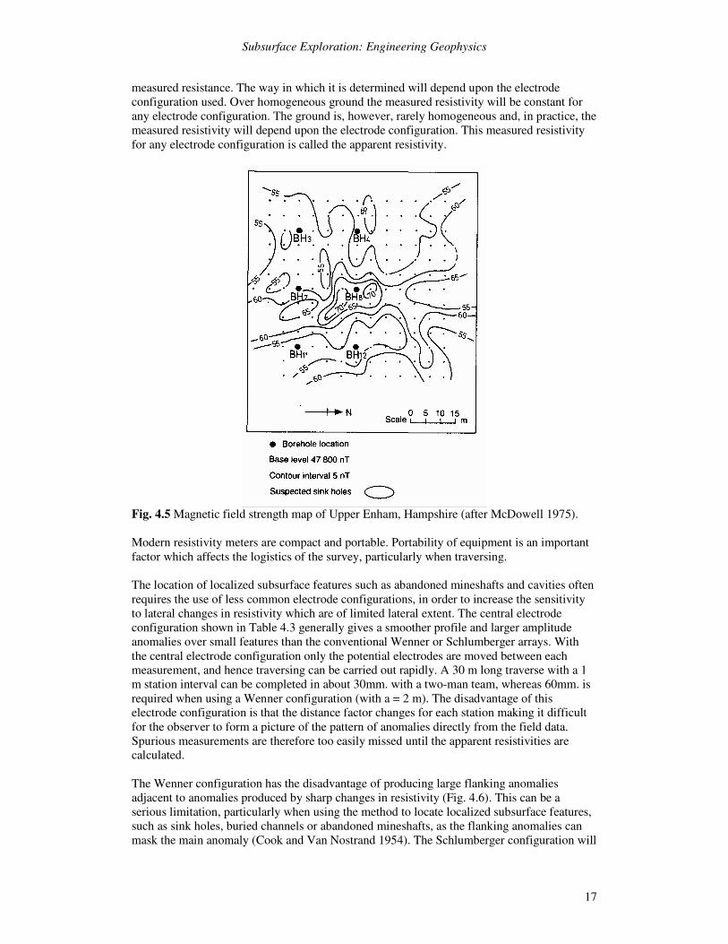
Fig. 4.4 Magnetic field strength map of Mangotsfield, Bristol (after Hooper and McDowell, 1977). The advantage of magnetic methods is the speed at which measurements can be taken. With a proton magnetometer it is possible to cover an area of 1500 m2 in a day taking measurements on a 1 m grid. It is possible to cover 1000 m2 in 60 mm taking measurements on a 2 m grid with the less sensitive fluxgate magnetometer (Dearman et a!. 1977). Since essentially only one correction is applied to the field measurements, data reduction, presentation and interpretation can be carried out rapidly. Clearly the magnetic methods can be most cost effective in site investigations that require localized features at shallow depths to be located provided of course that the conditions are recognized as being suitable for the method to have a reasonable chance of success. The main use of magnetic methods in site investigation appears to be for the location of abandoned mineshafts. The successful location of such features using magnetic methods has been reported by Raybould and Price (1966), Maxwell (1976), Dearman et al. (1977) and Hooper and McDowell (1977). It is unfortunate, however, that unsuccessful cases are not also reported, as these are equally (if not more) numerous than the successful cases. The publication of unsuccessful cases would give a better insight to some of the drawbacks of the method and perhaps allow some improvements to be made. The main problem in detecting abandoned shafts is that there is a great variety of anomalies associated with these features. Each shaft may be different from another in terms of:
Site Investigation
16
1. whether it is capped or uncapped: 2. the type of capping material; 3. the type of shaft lining; 4. the type of shaft infilling material (if present); 5. groundwater table; and 6. the nature of the surrounding debris.
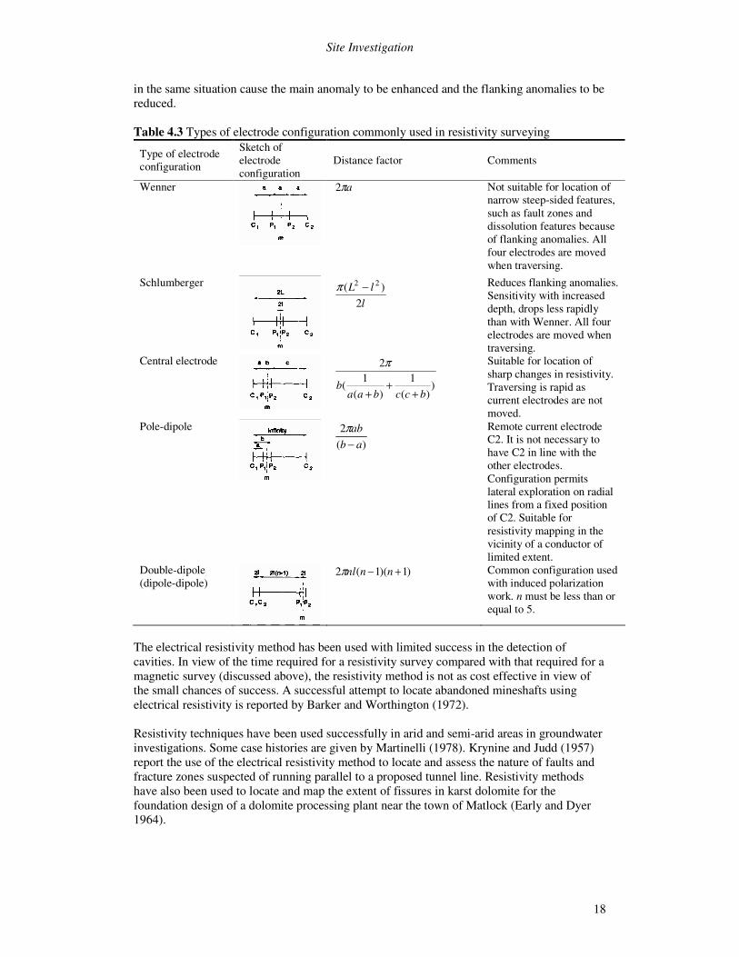
Thus all anomalies must be investigated by direct methods. Often the method is used in the wrong conditions, such as areas where the ground is particularly heterogeneous (which is not unusual in mining areas) or areas where there is likelihood of extraneous interference. The chances of success in such cases are minimal. The limitations of the method mentioned earlier clearly reduce the number of situations where success is possible. When using the magnetic methods to locate geological features it should be borne in mind that the method was initially developed for prospecting and was used to locate large-scale geological features. If the geology beneath a site is particularly complex, interpretation of magnetic data will be difficult, if not impossible, in extreme cases. Locally complex geology will also present problems in locating man-made features. McDowell (1975) discusses the use of magnetic methods in the detection of clay- filled sink holes in chalk. In favourable circumstances the proton precession magnetometer can be used to locate these features very rapidly and at little cost compared with employing direct methods of investigation, or other geophysical methods. A magnetic map for a test site in Upper Enham, Hampshire, is shown in Fig. 4.5. The magnetic method may also be used to locate basic igneous dykes below a cover of superficial deposits (Higginbottom 1976) and buried services such as clay or metal pipes. Electrical resistivity traversing Resistivity traversing is normally carried out to map horizontal changes in resistivity across a site. Lateral changes in resistivity are detected by using a fixed electrode separation and moving the whole electrode array between each resistivity. The interpretation of resistivity traverses is generally qualitative unless it is carried out in conjunction with sounding techniques. The use of traversing and sounding together is quite common in resistivity surveying (for example, see McDowell (1971)). The electrode configurations normally used in electrical traversing are the Wenner configuration and the Schlumberger configuration, Table 4.3. The Wenner configuration has the simplest geometry and is therefore easier to use and quicker than employing a Schlumberger configuration. If the resistivity station interval is the same as the electrode spacing it is possible to move from station to station along a traverse line by moving only one electrode each time. This is not possible with a Schlumberger configuration as the potential electrode spacing is not one-third of the current electrode spacing. Resistivity equipment passes a small low-frequency a.c. current (of up to 100 mA) to the ground via the current electrodes (C1 and C2). The resistance between the potential electrodes (P1 and P2) is determined by measuring the voltage between them. This voltage is normally amplified by the measuring device. The current source is then switched to an internal bridge circuit (via the amplifier) in which a resistance is altered using a potentiometer to give the same output voltage as measured between the potential electrodes. In general, as the electrode spacing is increased the measured resistance decreases. It is therefore necessary for the equipment to be capable of measuring small resistances. The resistances that may be measured with some a.c. devices are in the range 0.0003 � to 10 k� (ABEM Terrameter). The resistivity of the ground between the potential electrodes is determined from the
Subsurface Exploration: Engineering Geophysics
17
measured resistance. The way in which it is determined will depend upon the electrode configuration used. Over homogeneous ground the measured resistivity will be constant for any electrode configuration. The ground is, however, rarely homogeneous and, in practice, the measured resistivity will depend upon the electrode configuration. This measured resistivity for any electrode configuration is called the apparent resistivity.
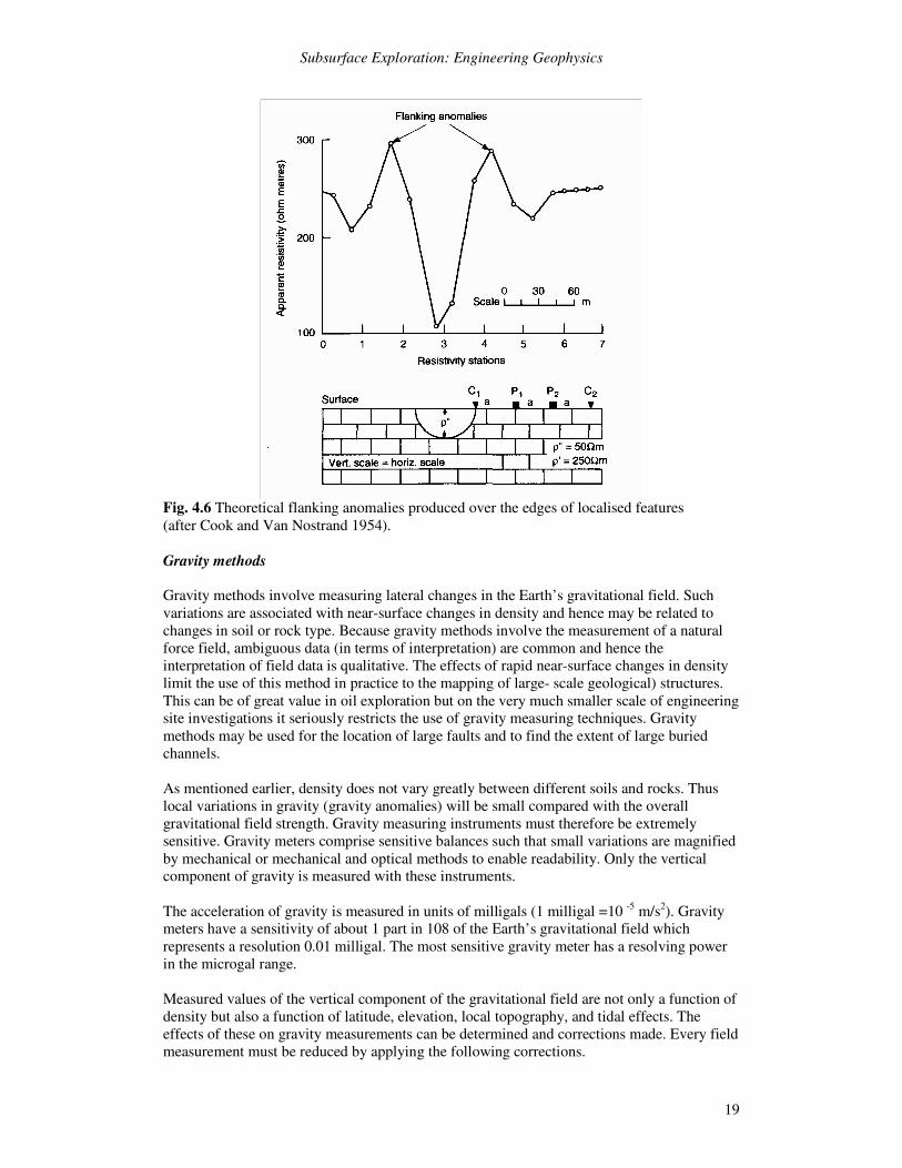
Fig. 4.5 Magnetic field strength map of Upper Enham, Hampshire (after McDowell 1975). Modern resistivity meters are compact and portable. Portability of equipment is an important factor which affects the logistics of the survey, particularly when traversing. The location of localized subsurface features such as abandoned mineshafts and cavities often requires the use of less common electrode configurations, in order to increase the sensitivity to lateral changes in resistivity which are of limited lateral extent. The central electrode configuration shown in Table 4.3 generally gives a smoother profile and larger amplitude anomalies over small features than the conventional Wenner or Schlumberger arrays. With the central electrode configuration only the potential electrodes are moved between each measurement, and hence traversing can be carried out rapidly. A 30 m long traverse with a 1 m station interval can be completed in about 30mm. with a two-man team, whereas 60mm. is required when using a Wenner configuration (with a = 2 m). The disadvantage of this electrode configuration is that the distance factor changes for each station making it difficult for the observer to form a picture of the pattern of anomalies directly from the field data. Spurious measurements are therefore too easily missed until the apparent resistivities are calculated. The Wenner configuration has the disadvantage of producing large flanking anomalies adjacent to anomalies produced by sharp changes in resistivity (Fig. 4.6). This can be a serious limitation, particularly when using the method to locate localized subsurface features, such as sink holes, buried channels or abandoned mineshafts, as the flanking anomalies can mask the main anomaly (Cook and Van Nostrand 1954). The Schlumberger configuration will
Site Investigation
18
in the same situation cause the main anomaly to be enhanced and the flanking anomalies to be reduced. Table 4.3 Types of electrode configuration commonly used in resistivity surveying
Type of electrode configuration
Sketch of electrode configuration
Distance factor Comments
Wenner
aπ2 Not suitable for location of narrow steep-sided features, such as fault zones and dissolution features because of flanking anomalies. All four electrodes are moved when traversing.
Schlumberger
llL
2)( 22 −π
Reduces flanking anomalies. Sensitivity with increased depth, drops less rapidly than with Wenner. All four electrodes are moved when traversing.
Central electrode
))(
1)(
1(
2
bccbaab
++
+
π
Suitable for location of sharp changes in resistivity. Traversing is rapid as current electrodes are not moved.
Pole-dipole
)(2
abab
−π
Remote current electrode C2. It is not necessary to have C2 in line with the other electrodes. Configuration permits lateral exploration on radial lines from a fixed position of C2. Suitable for resistivity mapping in the vicinity of a conductor of limited extent.
Double-dipole (dipole-dipole)
)1)(1(2 +− nnnlπ Common configuration used with induced polarization work. n must be less than or equal to 5.
The electrical resistivity method has been used with limited success in the detection of cavities. In view of the time required for a resistivity survey compared with that required for a magnetic survey (discussed above), the resistivity method is not as cost effective in view of the small chances of success. A successful attempt to locate abandoned mineshafts using electrical resistivity is reported by Barker and Worthington (1972). Resistivity techniques have been used successfully in arid and semi-arid areas in groundwater investigations. Some case histories are given by Martinelli (1978). Krynine and Judd (1957) report the use of the electrical resistivity method to locate and assess the nature of faults and fracture zones suspected of running parallel to a proposed tunnel line. Resistivity methods have also been used to locate and map the extent of fissures in karst dolomite for the foundation design of a dolomite processing plant near the town of Matlock (Early and Dyer 1964).
Subsurface Exploration: Engineering Geophysics
19
Fig. 4.6 Theoretical flanking anomalies produced over the edges of localised features (after Cook and Van Nostrand 1954). Gravity methods Gravity methods involve measuring lateral changes in the Earth’s gravitational field. Such variations are associated with near-surface changes in density and hence may be related to changes in soil or rock type. Because gravity methods involve the measurement of a natural force field, ambiguous data (in terms of interpretation) are common and hence the interpretation of field data is qualitative. The effects of rapid near-surface changes in density limit the use of this method in practice to the mapping of large- scale geological) structures. This can be of great value in oil exploration but on the very much smaller scale of engineering site investigations it seriously restricts the use of gravity measuring techniques. Gravity methods may be used for the location of large faults and to find the extent of large buried channels. As mentioned earlier, density does not vary greatly between different soils and rocks. Thus local variations in gravity (gravity anomalies) will be small compared with the overall gravitational field strength. Gravity measuring instruments must therefore be extremely sensitive. Gravity meters comprise sensitive balances such that small variations are magnified by mechanical or mechanical and optical methods to enable readability. Only the vertical component of gravity is measured with these instruments. The acceleration of gravity is measured in units of milligals (1 milligal =10 -5 m/s2). Gravity meters have a sensitivity of about 1 part in 108 of the Earth’s gravitational field which represents a resolution 0.01 milligal. The most sensitive gravity meter has a resolving power in the microgal range. Measured values of the vertical component of the gravitational field are not only a function of density but also a function of latitude, elevation, local topography, and tidal effects. The effects of these on gravity measurements can be determined and corrections made. Every field measurement must be reduced by applying the following corrections.
Site Investigation
20
1. Latitude correction. This is applied because the Earth is not a perfect sphere and
hence the gravitational force varies between the poles and the equator. 2. Elevation correction. This is applied to reduce all gravity measurements to a common
elevation. The correction is in two parts. (i) Free air correction. This is made for the displacement of the point of
observation above the reference level (usually ordnance datum O.D.). This requires the levelling of the gravity meter to within 0.05 m.
(ii) Bouguer correction. This is applied to remove the effect of the material between the gravity meter and the datum level. This requires the density of the material to be known (usually it is estimated).
3. Terrain correction. This is applied to remove the effects of the surrounding topography. The correction is obtained from a graphical determination of the gravity effect at the observation point of all hills and valleys. The correction is usually calculated to about 20km out from the station but where relief is low the survey area considered for this correction is reduced (Higginbottom 1976).
4. Instrument drift and tidal correction. These corrections are made by returning to a base station and measuring the field strength at frequent intervals during the survey.
The corrected gravity measurements are known collectively as Bouguer anomalies. A gravity survey requires an accurate topographic survey of the site and surrounding area to be carried out to enable some of the corrections to be applied to the field data. In the British Isles most of the topographic data necessary may be obtained from Ordnance Survey maps and plans. Each observation point must however be accurately levelled. Clearly the acquisition and reduction of gravity data are extremely time- consuming and hence expensive. The corrected gravity data are normally presented as a contoured gravity map (Isogal map). The contour values may represent Bouguer anomalies or residual gravity values. Residual gravity values are derived from the difference between the regional Bouguer anomaly and the local Bouguer anomaly. These gravity maps allow anomalies to be readily identified (if of sufficient magnitude) and thus target areas are defined for direct investigation. Figure 4.7 shows examples of the different forms of gravity maps. To enable detection of subsurface features the amplitude of the gravity anomaly produced must be at least 0.2 mgal. Most features of engineering interest produce anomalies which are much smaller than this and in most cases may be detected more efficiently by other geophysical methods. The main exception according to Higginbottom (1976) is the case of faults with displacements large enough to introduce materials of different density across the fault plane, but where the contrast between other physical properties is slight. A density contrast may also give rise to a P-wave velocity contrast. It would be easier therefore to use a seismic method such as seismic refraction if this were the case. The gravity method has been used to aid determination of the cross-section of an alluvium filled valley in North Wales (Fig. 4.7, see Griffiths and King (1965), for discussion) and the location of cavities (Colley 1963). In general, gravity methods are too slow and expensive to be cost effective in conventional site investigations. Only in rare circumstances are the use of gravity methods justified particularly as justification must normally be based on the limited information available at an early stage of the investigation.
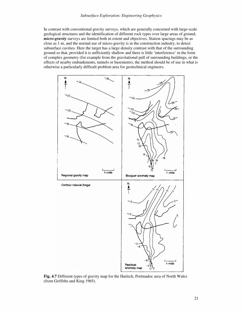
Subsurface Exploration: Engineering Geophysics
21
In contrast with conventional gravity surveys, which are generally concerned with large-scale geological structures and the identification of different rock types over large areas of ground, micro-gravity surveys are limited both in extent and objectives. Station spacings may be as close as 1 m, and the normal use of micro-gravity is in the construction industry, to detect subsurface cavities. Here the target has a large density contrast with that of the surrounding ground so that, provided it is sufficiently shallow and there is little ‘interference’ in the form of complex geometry (for example from the gravitational pull of surrounding buildings, or the effects of nearby embankments, tunnels or basements), the method should be of use in what is otherwise a particularly difficult problem area for geotechnical engineers.
Fig. 4.7 Different types of gravity map for the Harlech, Portmadoc area of North Wales (from Griffiths and King 1965).
Site Investigation
22
Typically, microgravity surveys may involve between 100 and 400 gravity stations with spacings as close as 1 m. The stations are levelled (using precise levelling equipment) and gravity measurements made to a resolution of 1 gal. Typical anomalies associated with shallow (0—l0m) features (e.g. voids, dissolution features and disturbed ground) are between 20 and 100 �gal. Using a portable PC, preliminary data processing may be carried out on site in order to confirm adequate definition of anomalies. PROFILING Most ground investigations will not make use of geophysical methods for profiling. This will normally be done by describing the material arising from boreholes, or by carrying out probing tests (Chapter 5). Exceptions may occur when there is need for information from areas between boreholes, or where boreholes are deep, and there is a need to correlate between them. Profiling can be carried out by identifying the characteristics of the material within each bed, or by identifying marker beds which are common to all boreholes. Whilst electrical resistivity can be used for this purpose, it is not common. Seismic probing is on the increase, and natural-gamma logging has long been used for inter- borehole correlations when deep investigations are being carried out. Electrical resistivity sounding Vertical changes in electrical resistivity are measured by progressively moving the electrodes outwards with respect to a fixed central point. The depth of current penetration is thus increased. Any variations in electrical resistivity with depth will be reflected in variations in measured potential difference. Electrical sounding involves investigating a progressively increasing volume of ground. As the vertical extent of this volume increases so will the lateral extent. Lateral variations in electrical resistivity will therefore introduce errors when determining variations of resistivity with depth. Ideally the lateral dimensions of the volume of ground under consideration should be kept relatively small compared with the vertical dimension. Electrical sounding using the Wenner configuration (Table 4.3) requires that both the current and potential electrode separations are increased between each resistivity measurement. The lateral dimensions are therefore allowed to become large. Thus Wenner sounding is likely to produce an erroneous resistivity/depth relationship because of lateral variations in resistivity. When electrical sounding with a Schlumberger configuration is used the potential electrode spacing is kept small (potential electrode spacing 0.2 current electrode spacing) and only the current electrode spacing is increased between each resistivity measurement. The potential electrode spacing is only increased when A V becomes very small and in this way the minimum lateral dimension condition is more-or-less satisfied. Thus the results of Schlumberger sounding are less prone to error due to lateral changes in resistivity. Figure 4.8 shows the effect of a lateral change in resistivity on the results of electrical sounding using Wenner and Schlumberger configurations. When using the Wenner array the errors due to lateral changes in resistivity may be greatly reduced and often eliminated by the use of the Offset Wenner system. The principles of this system may be summarized by considering the ‘signal contributions section’ for a Wenner array shown in Fig. 4.9. For homogeneous ground the positive and negative contributions of high magnitude cancel each other out and the resultant signal originates mainly from depth and not from the region around the electrodes. If, however, a high resistivity body (for example, a boulder) is located in the positive zone, the measured resistance will be greater than would have been measured in the absence of the body; if it is located in a negatively
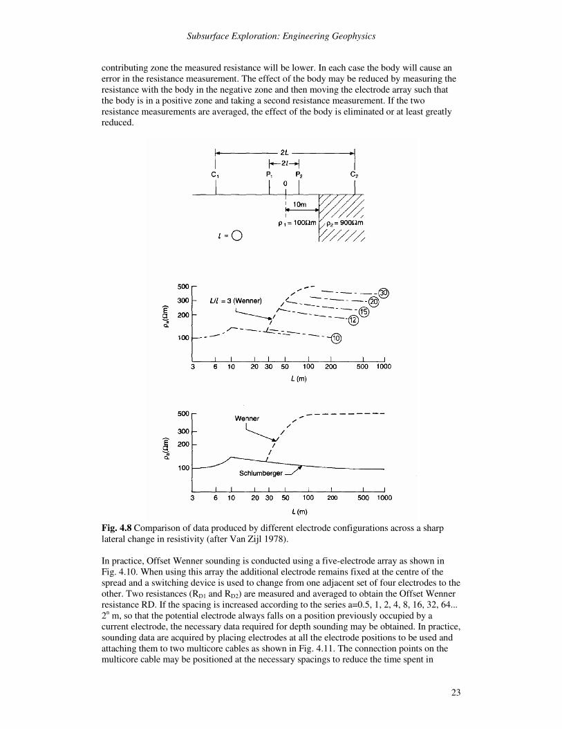
Subsurface Exploration: Engineering Geophysics
23
contributing zone the measured resistance will be lower. In each case the body will cause an error in the resistance measurement. The effect of the body may be reduced by measuring the resistance with the body in the negative zone and then moving the electrode array such that the body is in a positive zone and taking a second resistance measurement. If the two resistance measurements are averaged, the effect of the body is eliminated or at least greatly reduced.
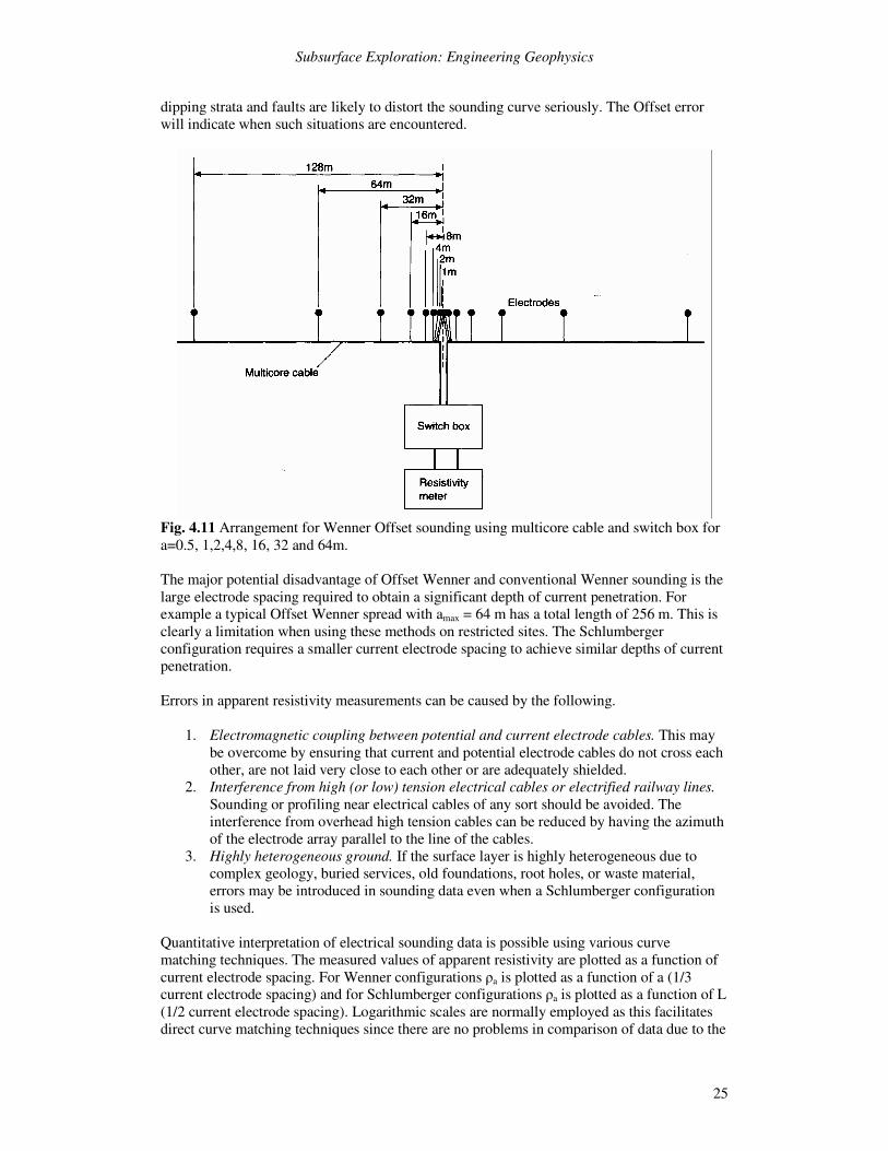
Fig. 4.8 Comparison of data produced by different electrode configurations across a sharp lateral change in resistivity (after Van Zijl 1978). In practice, Offset Wenner sounding is conducted using a five-electrode array as shown in Fig. 4.10. When using this array the additional electrode remains fixed at the centre of the spread and a switching device is used to change from one adjacent set of four electrodes to the other. Two resistances (RD1 and RD2) are measured and averaged to obtain the Offset Wenner resistance RD. If the spacing is increased according to the series a=0.5, 1, 2, 4, 8, 16, 32, 64... 2n m, so that the potential electrode always falls on a position previously occupied by a current electrode, the necessary data required for depth sounding may be obtained. In practice, sounding data are acquired by placing electrodes at all the electrode positions to be used and attaching them to two multicore cables as shown in Fig. 4.11. The connection points on the multicore cable may be positioned at the necessary spacings to reduce the time spent in
Site Investigation
24
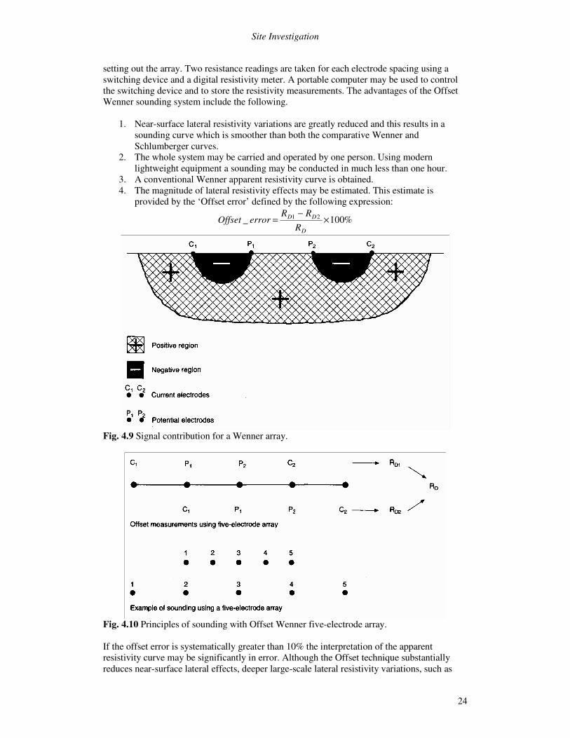
setting out the array. Two resistance readings are taken for each electrode spacing using a switching device and a digital resistivity meter. A portable computer may be used to control the switching device and to store the resistivity measurements. The advantages of the Offset Wenner sounding system include the following.
1. Near-surface lateral resistivity variations are greatly reduced and this results in a sounding curve which is smoother than both the comparative Wenner and Schlumberger curves.
2. The whole system may be carried and operated by one person. Using modern lightweight equipment a sounding may be conducted in much less than one hour.
3. A conventional Wenner apparent resistivity curve is obtained. 4. The magnitude of lateral resistivity effects may be estimated. This estimate is
provided by the ‘Offset error’ defined by the following expression:
%100_ 21 ×−
=D
DD
RRR
errorOffset
Fig. 4.9 Signal contribution for a Wenner array.
Fig. 4.10 Principles of sounding with Offset Wenner five-electrode array. If the offset error is systematically greater than 10% the interpretation of the apparent resistivity curve may be significantly in error. Although the Offset technique substantially reduces near-surface lateral effects, deeper large-scale lateral resistivity variations, such as
Subsurface Exploration: Engineering Geophysics
25
dipping strata and faults are likely to distort the sounding curve seriously. The Offset error will indicate when such situations are encountered.
Fig. 4.11 Arrangement for Wenner Offset sounding using multicore cable and switch box for a=0.5, 1,2,4,8, 16, 32 and 64m. The major potential disadvantage of Offset Wenner and conventional Wenner sounding is the large electrode spacing required to obtain a significant depth of current penetration. For example a typical Offset Wenner spread with amax = 64 m has a total length of 256 m. This is clearly a limitation when using these methods on restricted sites. The Schlumberger configuration requires a smaller current electrode spacing to achieve similar depths of current penetration. Errors in apparent resistivity measurements can be caused by the following.
1. Electromagnetic coupling between potential and current electrode cables. This may be overcome by ensuring that current and potential electrode cables do not cross each other, are not laid very close to each other or are adequately shielded.
2. Interference from high (or low) tension electrical cables or electrified railway lines. Sounding or profiling near electrical cables of any sort should be avoided. The interference from overhead high tension cables can be reduced by having the azimuth of the electrode array parallel to the line of the cables.
3. Highly heterogeneous ground. If the surface layer is highly heterogeneous due to complex geology, buried services, old foundations, root holes, or waste material, errors may be introduced in sounding data even when a Schlumberger configuration is used.
Quantitative interpretation of electrical sounding data is possible using various curve matching techniques. The measured values of apparent resistivity are plotted as a function of current electrode spacing. For Wenner configurations �a is plotted as a function of a (1/3 current electrode spacing) and for Schlumberger configurations �a is plotted as a function of L (1/2 current electrode spacing). Logarithmic scales are normally employed as this facilitates direct curve matching techniques since there are no problems in comparison of data due to the
Site Investigation
26
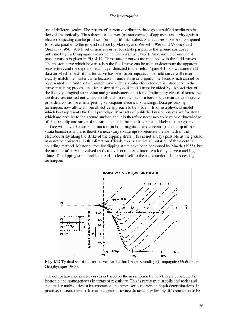
use of different scales. The pattern of current distribution through a stratified media can be derived theoretically. Thus theoretical curves (master curves) of apparent resistivity against electrode spacing can be produced (on logarithmic scales). Such curves have been computed for strata parallel to the ground surface by Mooney and Wetzel (1956) and Mooney and Orellana (1966). A full set of master curves for strata parallel to the ground surface is published by La Compagnie Générale de Géophysique (1963). An example of one set of master curves is given in Fig. 4.12. These master curves are matched with the field curves. The master curve which best matches the field curve can be used to determine the apparent resistivities and the depths of each layer detected in the field. Figure 4.13 shows some field data on which a best-fit master curve has been superimposed. The field curve will never exactly match the master curve because of undulating or dipping interfaces which cannot be represented in a finite set of master curves. Thus a subjective element is introduced in the curve matching process and the choice of physical model must be aided by a knowledge of the likely geological succession and groundwater conditions. Preliminary electrical soundings are therefore carried out where possible close to the site of a borehole or near an exposure to provide a control over interpreting subsequent electrical soundings. Data processing techniques now allow a more objective approach to be made in finding a physical model which best represents the field prototype. Most sets of published master curves are for strata which are parallel to the ground surface and it is therefore necessary to have prior knowledge of the local dip and strike of the strata beneath the site. It is most unlikely that the ground surface will have the same inclination (in both magnitude and direction) as the dip of the strata beneath it and it is therefore necessary to attempt to orientate the azimuth of the electrode array along the strike of the dipping strata. This is not always possible as the ground may not be horizontal in this direction. Clearly this is a serious limitation of the electrical sounding method. Master curves for dipping strata have been computed by Maeda (1955), but the number of curves involved tends to over-complicate interpretation by curve matching alone. The dipping strata problem tends to lend itself to the more modern data processing techniques.
Fig. 4.12 Typical set of master curves for Schlumberger sounding (Compagnie Générale de Géophysique 1963). The computation of master curves is based on the assumption that each layer considered is isotropic and homogeneous in terms of resistivity. This is rarely true in soils and rocks and can lead to ambiguities in interpretation and hence serious errors in depth determinations. In practice, measurements taken at the ground surface do not allow for any differentiation to be
Subsurface Exploration: Engineering Geophysics
27
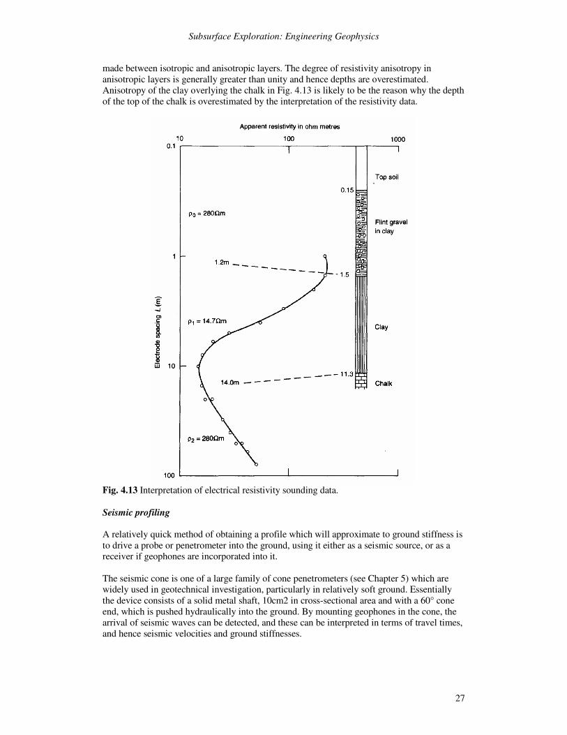
made between isotropic and anisotropic layers. The degree of resistivity anisotropy in anisotropic layers is generally greater than unity and hence depths are overestimated. Anisotropy of the clay overlying the chalk in Fig. 4.13 is likely to be the reason why the depth of the top of the chalk is overestimated by the interpretation of the resistivity data.
Fig. 4.13 Interpretation of electrical resistivity sounding data. Seismic profiling A relatively quick method of obtaining a profile which will approximate to ground stiffness is to drive a probe or penetrometer into the ground, using it either as a seismic source, or as a receiver if geophones are incorporated into it. The seismic cone is one of a large family of cone penetrometers (see Chapter 5) which are widely used in geotechnical investigation, particularly in relatively soft ground. Essentially the device consists of a solid metal shaft, 10cm2 in cross-sectional area and with a 60° cone end, which is pushed hydraulically into the ground. By mounting geophones in the cone, the arrival of seismic waves can be detected, and these can be interpreted in terms of travel times, and hence seismic velocities and ground stiffnesses.

Site Investigation
28
Figure 4.14 shows the principle of the test method. A seismic piezocone is pushed progressively into the ground. Each metre or so it is stopped. A hammer is used at the surface, to produce seismic waves. For shallow saturated soil the compressional (P) wave velocity is normally primarily a function of the bulk modulus of the pore water, and is not sensitive to changes in the stiffness of the soil skeleton. Shear waves are usually used, and are typically generated by placing a wooden sleeper under the wheel of the penetrometer truck and striking it horizontally with a large hammer.
Fig. 4.14 Principle of seismic shear wave profiling using the cone penetrometer (courtesy Fugro). The striking of the block with the hammer triggers an armed seismograph, and this records the arrival of the seismic waves at the cone tip. If the site is noisy, the signal- to-noise ratio can be improved by repeating the process and stacking the signals. The travel time from the surface to each cone position is determined from the seismograph traces, and the time taken for the wave to travel between each cone position is determined by subtraction. The so-called ‘interval velocity’ is then determined by dividing this difference in travel time by the distance between the two cone positions. Better results can be obtained by using a cone with two sets of geophones, mounted a metre or so apart, in it. Finally, the very small strain shear modulus of the soil can be determined from the equation:
2sVG ρ=
� (4.5)
where � = soil density, which can either be estimated or determined from samples, and Vs = seismic shear wave velocity. Figure 4.15 shows a comparison of shear wave velocities determined both by the seismic cone and by a cross-hole test (see later), compared with the cone resistance itself.
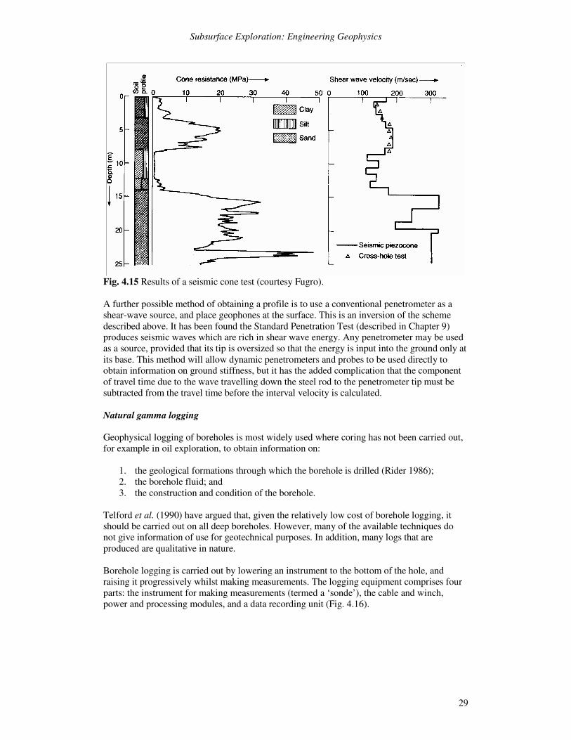
Subsurface Exploration: Engineering Geophysics
29
Fig. 4.15 Results of a seismic cone test (courtesy Fugro). A further possible method of obtaining a profile is to use a conventional penetrometer as a shear-wave source, and place geophones at the surface. This is an inversion of the scheme described above. It has been found the Standard Penetration Test (described in Chapter 9) produces seismic waves which are rich in shear wave energy. Any penetrometer may be used as a source, provided that its tip is oversized so that the energy is input into the ground only at its base. This method will allow dynamic penetrometers and probes to be used directly to obtain information on ground stiffness, but it has the added complication that the component of travel time due to the wave travelling down the steel rod to the penetrometer tip must be subtracted from the travel time before the interval velocity is calculated. Natural gamma logging Geophysical logging of boreholes is most widely used where coring has not been carried out, for example in oil exploration, to obtain information on:
1. the geological formations through which the borehole is drilled (Rider 1986); 2. the borehole fluid; and 3. the construction and condition of the borehole.
Telford et al. (1990) have argued that, given the relatively low cost of borehole logging, it should be carried out on all deep boreholes. However, many of the available techniques do not give information of use for geotechnical purposes. In addition, many logs that are produced are qualitative in nature. Borehole logging is carried out by lowering an instrument to the bottom of the hole, and raising it progressively whilst making measurements. The logging equipment comprises four parts: the instrument for making measurements (termed a ‘sonde’), the cable and winch, power and processing modules, and a data recording unit (Fig. 4.16).
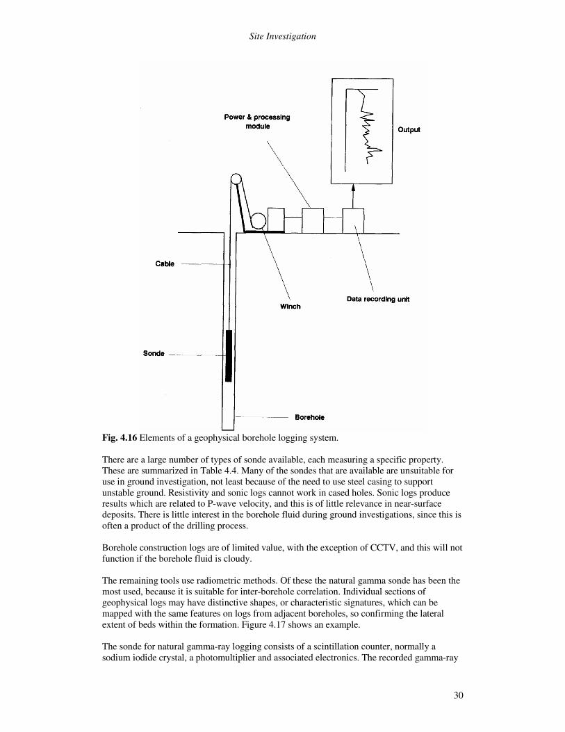
Site Investigation
30
Fig. 4.16 Elements of a geophysical borehole logging system. There are a large number of types of sonde available, each measuring a specific property. These are summarized in Table 4.4. Many of the sondes that are available are unsuitable for use in ground investigation, not least because of the need to use steel casing to support unstable ground. Resistivity and sonic logs cannot work in cased holes. Sonic logs produce results which are related to P-wave velocity, and this is of little relevance in near-surface deposits. There is little interest in the borehole fluid during ground investigations, since this is often a product of the drilling process. Borehole construction logs are of limited value, with the exception of CCTV, and this will not function if the borehole fluid is cloudy. The remaining tools use radiometric methods. Of these the natural gamma sonde has been the most used, because it is suitable for inter-borehole correlation. Individual sections of geophysical logs may have distinctive shapes, or characteristic signatures, which can be mapped with the same features on logs from adjacent boreholes, so confirming the lateral extent of beds within the formation. Figure 4.17 shows an example. The sonde for natural gamma-ray logging consists of a scintillation counter, normally a sodium iodide crystal, a photomultiplier and associated electronics. The recorded gamma-ray
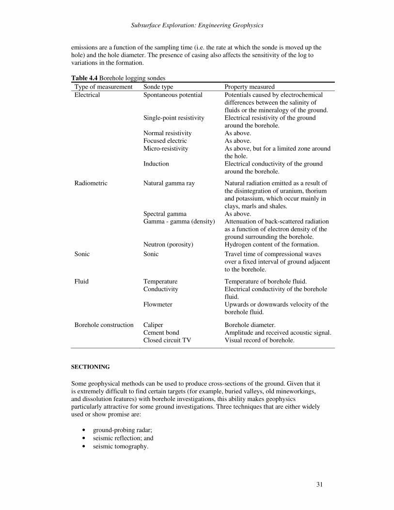
Subsurface Exploration: Engineering Geophysics
31
emissions are a function of the sampling time (i.e. the rate at which the sonde is moved up the hole) and the hole diameter. The presence of casing also affects the sensitivity of the log to variations in the formation. Table 4.4 Borehole logging sondes Type of measurement Sonde type Property measured Electrical Spontaneous potential
Single-point resistivity Normal resistivity Focused electric Micro-resistivity Induction
Potentials caused by electrochemical differences between the salinity of fluids or the mineralogy of the ground. Electrical resistivity of the ground around the borehole. As above. As above. As above, but for a limited zone around the hole. Electrical conductivity of the ground around the borehole.
Radiometric Natural gamma ray Spectral gamma Gamma - gamma (density) Neutron (porosity)
Natural radiation emitted as a result of the disintegration of uranium, thorium and potassium, which occur mainly in clays, marls and shales. As above. Attenuation of back-scattered radiation as a function of electron density of the ground surrounding the borehole. Hydrogen content of the formation.
Sonic Sonic Travel time of compressional waves over a fixed interval of ground adjacent to the borehole.
Fluid Temperature Conductivity Flowmeter
Temperature of borehole fluid. Electrical conductivity of the borehole fluid. Upwards or downwards velocity of the borehole fluid.
Borehole construction Caliper Cement bond Closed circuit TV
Borehole diameter. Amplitude and received acoustic signal. Visual record of borehole.
SECTIONING Some geophysical methods can be used to produce cross-sections of the ground. Given that it is extremely difficult to find certain targets (for example, buried valleys, old mineworkings, and dissolution features) with borehole investigations, this ability makes geophysics particularly attractive for some ground investigations. Three techniques that are either widely used or show promise are:
• ground-probing radar; • seismic reflection; and • seismic tomography.
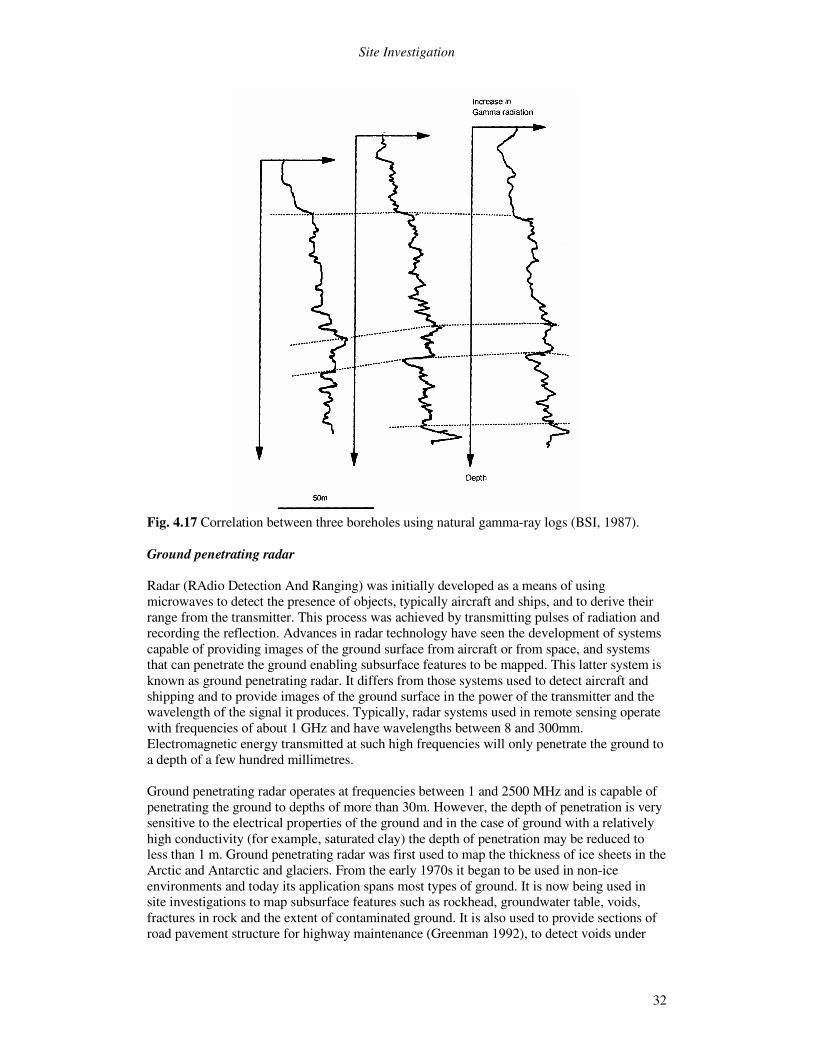
Site Investigation
32
Fig. 4.17 Correlation between three boreholes using natural gamma-ray logs (BSI, 1987). Ground penetrating radar Radar (RAdio Detection And Ranging) was initially developed as a means of using microwaves to detect the presence of objects, typically aircraft and ships, and to derive their range from the transmitter. This process was achieved by transmitting pulses of radiation and recording the reflection. Advances in radar technology have seen the development of systems capable of providing images of the ground surface from aircraft or from space, and systems that can penetrate the ground enabling subsurface features to be mapped. This latter system is known as ground penetrating radar. It differs from those systems used to detect aircraft and shipping and to provide images of the ground surface in the power of the transmitter and the wavelength of the signal it produces. Typically, radar systems used in remote sensing operate with frequencies of about 1 GHz and have wavelengths between 8 and 300mm. Electromagnetic energy transmitted at such high frequencies will only penetrate the ground to a depth of a few hundred millimetres. Ground penetrating radar operates at frequencies between 1 and 2500 MHz and is capable of penetrating the ground to depths of more than 30m. However, the depth of penetration is very sensitive to the electrical properties of the ground and in the case of ground with a relatively high conductivity (for example, saturated clay) the depth of penetration may be reduced to less than 1 m. Ground penetrating radar was first used to map the thickness of ice sheets in the Arctic and Antarctic and glaciers. From the early 1970s it began to be used in non-ice environments and today its application spans most types of ground. It is now being used in site investigations to map subsurface features such as rockhead, groundwater table, voids, fractures in rock and the extent of contaminated ground. It is also used to provide sections of road pavement structure for highway maintenance (Greenman 1992), to detect voids under
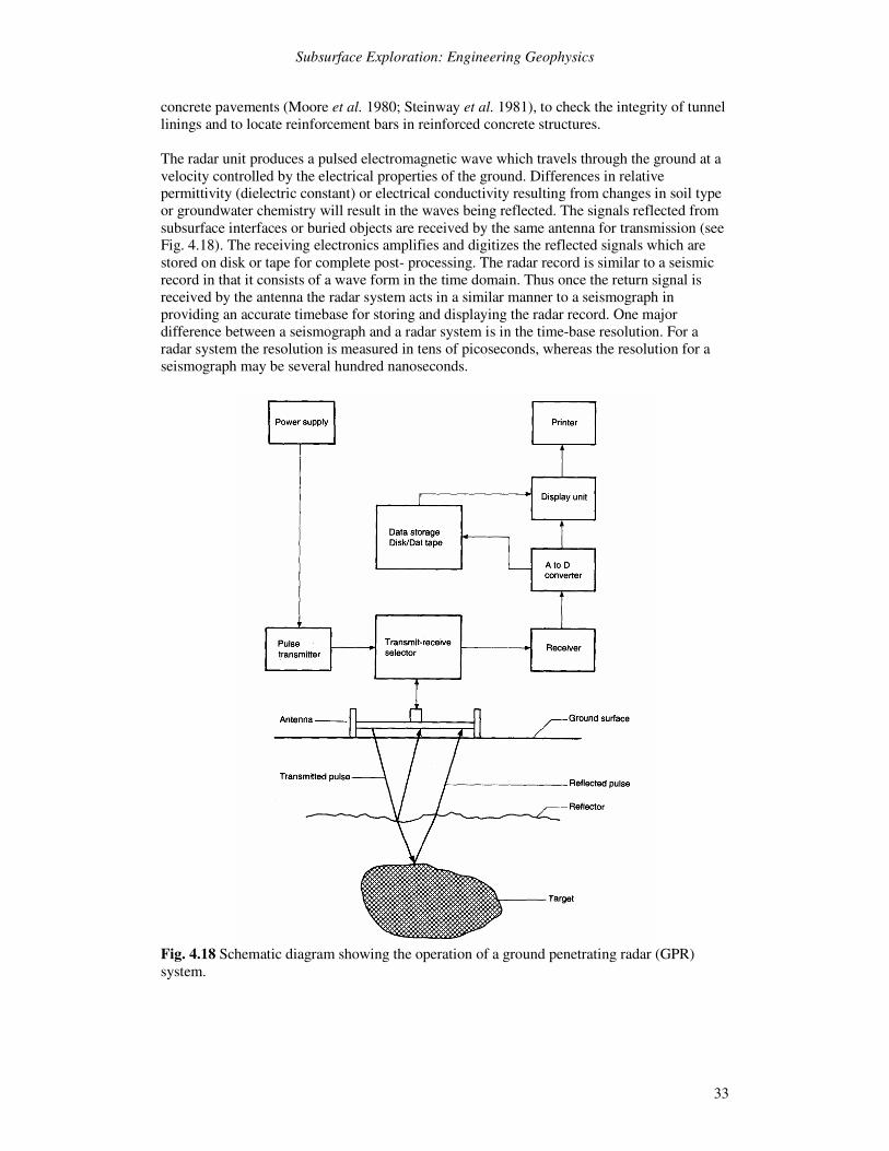
Subsurface Exploration: Engineering Geophysics
33
concrete pavements (Moore et al. 1980; Steinway et al. 1981), to check the integrity of tunnel linings and to locate reinforcement bars in reinforced concrete structures. The radar unit produces a pulsed electromagnetic wave which travels through the ground at a velocity controlled by the electrical properties of the ground. Differences in relative permittivity (dielectric constant) or electrical conductivity resulting from changes in soil type or groundwater chemistry will result in the waves being reflected. The signals reflected from subsurface interfaces or buried objects are received by the same antenna for transmission (see Fig. 4.18). The receiving electronics amplifies and digitizes the reflected signals which are stored on disk or tape for complete post- processing. The radar record is similar to a seismic record in that it consists of a wave form in the time domain. Thus once the return signal is received by the antenna the radar system acts in a similar manner to a seismograph in providing an accurate timebase for storing and displaying the radar record. One major difference between a seismograph and a radar system is in the time-base resolution. For a radar system the resolution is measured in tens of picoseconds, whereas the resolution for a seismograph may be several hundred nanoseconds.
Fig. 4.18 Schematic diagram showing the operation of a ground penetrating radar (GPR) system.
Site Investigation
34
Immediate on-site results may be viewed on a graphics display. Modern radar systems such as the SIR System-10 manufactured by GSSI (Geophysical Survey Systems Inc.) may be controlled from a PC and have a colour display which aids interpretation. Such systems also allow signal enhancement by algebraic addition of successive records taken at the same location. This process, known as stacking, improves the signal-to-noise ratio. It is a feature that is also found on most modern seismographs. By moving the radar antenna over the ground surface a continuous real-time geological section (pseudo-section) is built up by arranging each radar record next to each other. A typical pseudo-section is shown in Fig. 4.19. The horizontal axis of the section represents distance and the vertical axis represents the two-way travel times of reflections in nanoseconds. In order to transform this into distance the velocity must be known. The lines shown on the pseudo-section represent reflectors and are made up from coalescing wiggle traces from individual radar records.
Fig. 4.19 Radar pseudo-section showing sands overlying limestone (after Ulriksen 1983). The section shown in Fig. 4.19 depicts sands overlying limestone. The diagram shows the unique capacity of the radar to display the stratification in soils. The upper part of the section consists of wind-blown sands which are characterized by some disorder. The underlying sand is more regularly stratified indicating deposition under water. The limestone in the bottom of the section appears dark. In order to interpret a radar pseudo-section it is necessary to know how the section is derived. Figure 4.20 illustrates schematically the typical format of a radar reflection section. The physical model used in Fig. 4.20 depicts a horizontal reflector overlying an isolated target. Such a model may be represented in the field by a cavity in, say, limestone which is overlain by soil. The transmitted pulse from the radar antenna does not travel vertically downward but spreads out in a cone. This means that the isolated target is ‘seen’ before the antenna is directly over it. A relatively small void or isolated reflector will act like a point target which produces a characteristic hyperbolic anomaly. Measurements of travel time on the hyperbolic tails of this anomaly may be used to calculate the depth of the feature at the point when the antenna is vertically above it. Unless the buried feature is made of conducting material, such as metal the electromagnetic waves will pass
Subsurface Exploration: Engineering Geophysics
35
through the feature and be reflected from the bottom as well as the top as shown in Fig. 4.20. These reflections may permit the size of the buried feature to be determined. Figure 4.21 shows a radar pseudo-section of cavities in limestone.
Fig. 4.20 Schematic illustration of the format of a GPR reflection section. The horizontal reflector shown in Fig. 4.20 appears as a linear anomaly in the pseudo-section. The depth of this reflector can only be determined if the velocity of the material above it is known. Velocity analysis can be done by physically sampling the material and performing the appropriate laboratory tests. However, this approach is time consuming and expensive. One of the simplest and most common methods used for velocity determination is common-mid-point (CMP) sounding which is used in reflection seismic. There are two requirements for this method to be applicable:
1. there must be a planar reflector extended for some distance along the profile; 2. there must be two antennas, one transmitting and one receiving.
The arrangement is shown in Fig. 4.22. By moving both antennas equal distances away from the initial centre point the same reflection point will be maintained. The depth to the reflector can now be calculated using the expression:
Site Investigation
36
���
�
�
−−
=)(4 2
22
1
22
21
21
22
tt
xtxtz (4.6)
With the depth known, the average velocity in the material is calculated using the travel time when the antenna separation was zero.
Fig. 4.21 Radar profile showing cavities in limestone (after Ulriksen 1983). The radar pseudo-sections have a compressed x-axis, which makes them look more dramatic than the recorded structures actually are. Some inclined reflectors may be lost from the section as the dip exceeds a critical value. The maximum recordable slope is identical to the radiation angle of the antenna. This is not a fixed measure but rather a matter of detection level in the receiver. For practical purposes it may be regarded as an angle. Ulriksen (1983) found the maximum recordable slope angle for an 80 MHz antenna (used as both transmitter and receiver) in peat was 36°. Near-surface soil may contain a great number of minor reflectors which cause scattering of the return signal and makes the sections difficult to-interpret. This problem is overcome by using two separated antennas. One antenna is used as a transmitter and the other is used as a receiver. The near-surface echoes will be returned to the transmitter rather than to the receiver antenna. Echoes from greater depths will thus be enhanced. There are a number of similarities between the theory of electromagnetic and elastic body (seismic) wave propagation (Ursin 1983). Both radar and acoustic pulses propagate with finite velocities that depend on the material properties and each are reflected and diffracted by local changes in the medium. The dynamic behaviours are different (with regard to amplitude and dispersion), but the kinematic behaviours are the same. This similarity results from the fact that displacement currents dominate conductive currents at frequencies where GPR is effective. Under these conditions, an electromagnetic pulse propagates with virtually no dispersion and has a velocity controlled by the dielectric properties of the material alone. For equal wavelengths there is considerably less attenuation of electromagnetic energy than of mechanical energy. At low frequencies or in high conductivity environments (for example, sand saturated with saline water) where conductivity currents dominate, GPR cannot be used
Subsurface Exploration: Engineering Geophysics
37
effectively. In such cases electromagnetic fields diffuse into the ground and electromagnetic induction methods (for example, transient EM) are more appropriate as a means of investigation.
Fig. 4.22 Illustration of CMP sounding. The similarities between radar and reflection seismics have resulted in data-processing techniques that were developed for the latter (such as convolution and migration) being used for processing radar data. The major factors that affect the performance of ground penetrating radar are: 1. the contrast in relative permittivity (dialectric constant) between the target and the
surrounding ground; 2. the conductivity of the ground; 3. the shape of the target and its orientation with respect to the radar antenna; and 4. the density of scattering bodies within the ground that produce reflection similar to those
from the target.
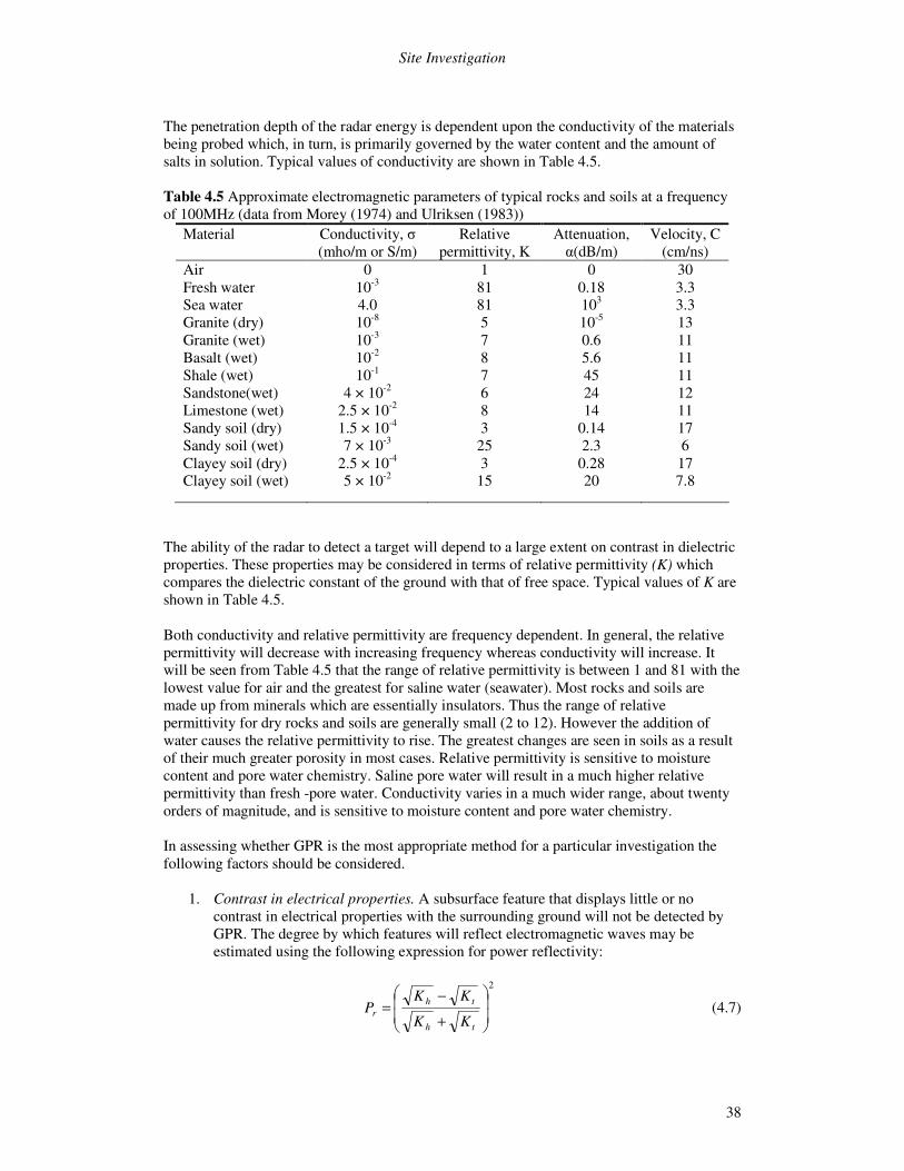
Site Investigation
38
The penetration depth of the radar energy is dependent upon the conductivity of the materials being probed which, in turn, is primarily governed by the water content and the amount of salts in solution. Typical values of conductivity are shown in Table 4.5. Table 4.5 Approximate electromagnetic parameters of typical rocks and soils at a frequency of 100MHz (data from Morey (1974) and Ulriksen (1983))
Material Conductivity, � (mho/m or S/m)
Relative permittivity, K
Attenuation, �(dB/m)
Velocity, C (cm/ns)
Air Fresh water Sea water Granite (dry) Granite (wet) Basalt (wet) Shale (wet) Sandstone(wet) Limestone (wet) Sandy soil (dry) Sandy soil (wet) Clayey soil (dry) Clayey soil (wet)
0 10-3 4.0 10-8 10-3 10-2 10-1
4 × 10⁻² 2.5 × 10⁻² 1.5 × 10⁻⁴ 7 × 10⁻³
2.5 × 10⁻⁴ 5 × 10⁻²
1 81 81 5 7 8 7 6 8 3
25 3
15
0 0.18 103 10-5 0.6 5.6 45 24 14
0.14 2.3
0.28 20
30 3.3 3.3 13 11 11 11 12 11 17 6
17 7.8
The ability of the radar to detect a target will depend to a large extent on contrast in dielectric properties. These properties may be considered in terms of relative permittivity (K) which compares the dielectric constant of the ground with that of free space. Typical values of K are shown in Table 4.5. Both conductivity and relative permittivity are frequency dependent. In general, the relative permittivity will decrease with increasing frequency whereas conductivity will increase. It will be seen from Table 4.5 that the range of relative permittivity is between 1 and 81 with the lowest value for air and the greatest for saline water (seawater). Most rocks and soils are made up from minerals which are essentially insulators. Thus the range of relative permittivity for dry rocks and soils are generally small (2 to 12). However the addition of water causes the relative permittivity to rise. The greatest changes are seen in soils as a result of their much greater porosity in most cases. Relative permittivity is sensitive to moisture content and pore water chemistry. Saline pore water will result in a much higher relative permittivity than fresh -pore water. Conductivity varies in a much wider range, about twenty orders of magnitude, and is sensitive to moisture content and pore water chemistry. In assessing whether GPR is the most appropriate method for a particular investigation the following factors should be considered.
1. Contrast in electrical properties. A subsurface feature that displays little or no contrast in electrical properties with the surrounding ground will not be detected by GPR. The degree by which features will reflect electromagnetic waves may be estimated using the following expression for power reflectivity:
2
��
�
�
��
�
�
+
−=
th
thr
KK
KKP (4.7)
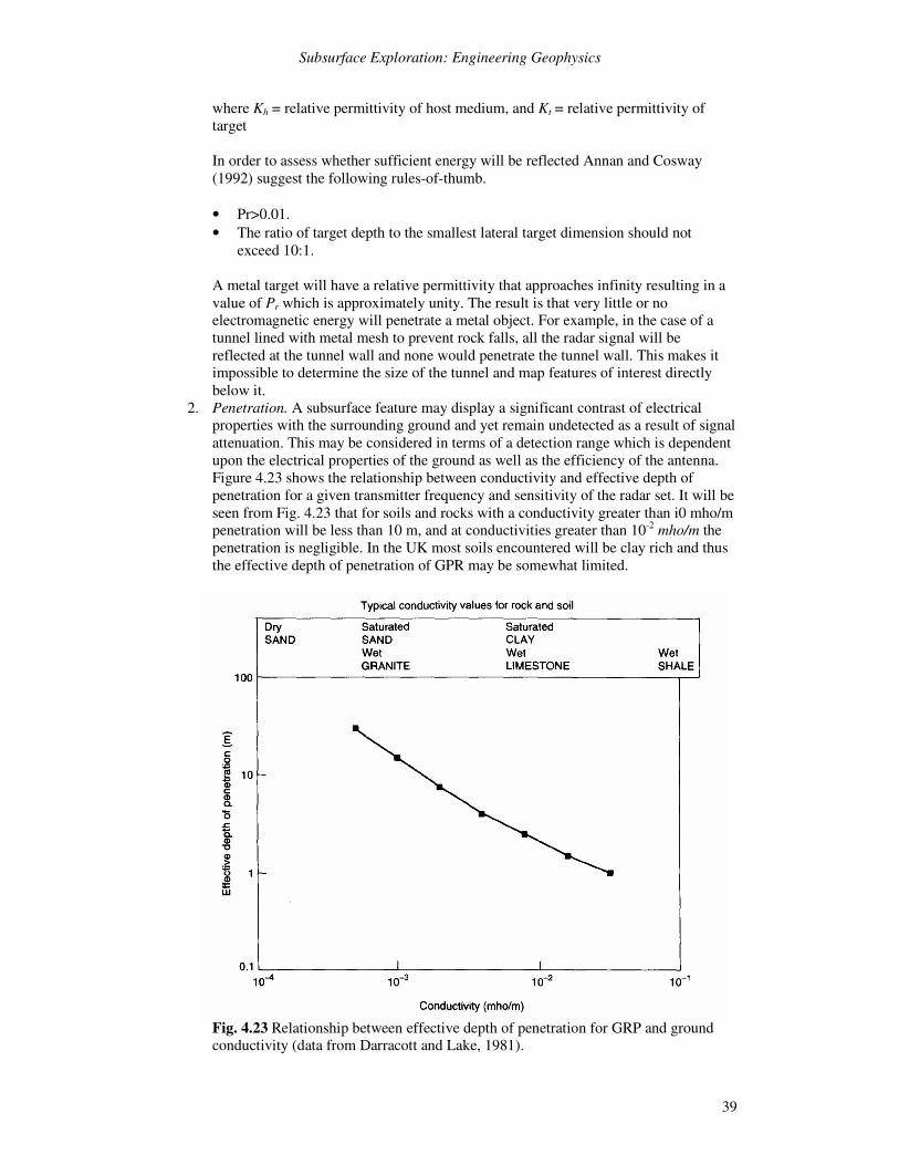
Subsurface Exploration: Engineering Geophysics
39
where Kh = relative permittivity of host medium, and Kt = relative permittivity of target
In order to assess whether sufficient energy will be reflected Annan and Cosway (1992) suggest the following rules-of-thumb.
• Pr>0.01. • The ratio of target depth to the smallest lateral target dimension should not
exceed 10:1.
A metal target will have a relative permittivity that approaches infinity resulting in a value of Pr which is approximately unity. The result is that very little or no electromagnetic energy will penetrate a metal object. For example, in the case of a tunnel lined with metal mesh to prevent rock falls, all the radar signal will be reflected at the tunnel wall and none would penetrate the tunnel wall. This makes it impossible to determine the size of the tunnel and map features of interest directly below it.
2. Penetration. A subsurface feature may display a significant contrast of electrical properties with the surrounding ground and yet remain undetected as a result of signal attenuation. This may be considered in terms of a detection range which is dependent upon the electrical properties of the ground as well as the efficiency of the antenna. Figure 4.23 shows the relationship between conductivity and effective depth of penetration for a given transmitter frequency and sensitivity of the radar set. It will be seen from Fig. 4.23 that for soils and rocks with a conductivity greater than i0 mho/m penetration will be less than 10 m, and at conductivities greater than 10-2 mho/m the penetration is negligible. In the UK most soils encountered will be clay rich and thus the effective depth of penetration of GPR may be somewhat limited.
Fig. 4.23 Relationship between effective depth of penetration for GRP and ground conductivity (data from Darracott and Lake, 1981).
Site Investigation
40
As a rough guide to estimating the effective penetration depth (Lmax) Annan and Cosway (1992) suggest the following rule-of-thumb:
σα3530
maxmax << orLL (4.8)
where �= attenuation in dB/m, and � = conductivity in mS/m. These equations are generally applicable where attenuation is moderate to high (>0.1 dB/m) which is typical of most geological settings. The values of Lmax vary according to whether conductivity or attenuation is used in the calculation. For example Lmax for a wet clayey soil will be 0.7m based on conductivity, and 1.5m based on attenuation.
3. Resolution. The spatial resolution of GPR is related to the wavelength of the electromagnetic waves it produces. As the wavelength is increased, the resolution of the radar is reduced. Ideally the wavelength should be short in relation to the illuminated objects. The operating frequency of radar together with the electrical properties of the ground will determine the wavelength of electromagnetic waves passing through it. For example, an 80MHz antenna has a wavelength of 3.45m in air and 0.42m in freshwater. For a given transmitter power rating the depth of penetration will be influenced by the operating frequency of the radar. The depth of penetration may be increased by reducing the operational frequency at the expense of resolution. Annan and Cosway (1992) provide a simple guide for determining penetration depth for a given frequency based on the assumption that the spatial resolution required is about 25% of the target depth. This guide is shown in Table 4.6. In cases where maximum resolution is required near the ground surface as well as at depth it will be necessary to carry out separate surveys using antennas with different operating frequencies.
4. Signal-to-noise ratio. The GPR method is sensitive to the environment in which the survey is carried out. Metal structures, radio transmitters, overhead or underground electrical power lines may all produce sufficient noise to saturate a sensitive receiver.
Table 4.6 Guide for determining
penetration depth for a given frequency
Depth (m)
Centre frequency (MHz)
0.5 1000 1.0 500 2.0 200 5.0 100 10.0 50 30.0 25 50.0 10
In general, GPR methods can be used more cost effectively in situations when searching for a known target (for example, buried pipe, subsurface cavities, rock ledge, buried valley, etc.) rather than as a general reconnaissance tool, where broad conclusions about subsurface conditions are sought. A comprehensive review of the application of ground penetrating radar to civil engineering is given by Ulriksen (1983). Case histories illustrating the use of GPR in the UK are given by Darracot and Lake (1981) and Leggo and Leech (1983).
Subsurface Exploration: Engineering Geophysics
41
Seismic reflection Seismic reflection methods have been used on offshore site investigations since the 1950s. Traditionally this method has not been used for conventional, onshore investigations because of the relatively low cost of boreholes compared with those offshore, and because the method has in the past been difficult to apply to shallow investigations. Recent research has extended the method to shallow depths, but it has yet to find application in onshore civil engineering ground investigations. The seismic reflection method is used in engineering investigations primarily for accurate profiling of geological structures. The method has the unique advantage of permitting mapping of many horizons from a single shot, and the precision of mapping does not decrease significantly with depth in favourable conditions. This is not the case with other geophysical methods. Both quantitative and qualitative interpretations of reflection data are possible. The seismic reflection method relies on measuring travel times of P waves which have been reflected back to the surface by boundaries separating materials with different characteristic P-wave velocities. The proportion of energy reflected by a velocity interface is defined by the reflection coefficient of that interface. According to Dohr (1975) the reflection coefficient of an interface for a normally incident (i.e. the angle of incidence is zero) wave is:
0011
00111,0 VV
VVAA
Rd
r
ρρρρ
+−
== (4.9)
where Ar = amplitude of the reflected wave, Ad = amplitude of the normally incident wave, �o = density of upper layer, �1 = density of lower layer, V0= P-wave velocity of upper layer, and V1 = P-wave velocity of lower layer. Clearly the greater the reflection coefficient, the stronger the reflections are from the interface and hence more easily identified from the seismic record. As the density of rocks and soils is not very variable, velocity contrast must be the controlling factor with respect to the amplitude of reflected events. Telford et al. (1990) give the following values of R:
Interface R Sandstone on limestone 0.040 Soft ocean bottom 0.11 Base of weathering 0.46
Velocity inversions give rise to a negative reflection coefficient. This means that reflected waves will be 1800 out of phase with the incident waves. Complete phase reversals of this kind can be detected on the seismic record. Theoretically, therefore, it is possible to overcome the blind-zone problem in refraction surveying by careful examination of reflected events on the seismic record. In practice, however, such events may be difficult to identify at shallow depths. Interpretation of seismic reflection data can lead to accurate determinations of the depth and dip of the strata identified from the seismic record. This is only possible if the P-wave velocity of each layer is known. The P-wave velocity for each layer encountered may be determined by borehole methods or by analytical methods using travel-time data from the survey itself.
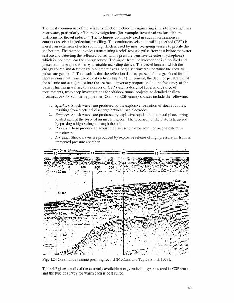
Site Investigation
42
The most common use of the seismic reflection method in engineering is in site investigations over water, particularly offshore investigations (for example, investigations for offshore platforms for the oil industry). The technique commonly used in such investigations is continuous seismic (reflection) profiling. The continuous seismic profiling method (CSP) is merely an extension of echo sounding which is used by most sea-going vessels to profile the sea bottom. The method involves transmitting a brief acoustic pulse from just below the water surface and detecting the reflected pulses with a pressure-sensitive detector (hydrophone) which is mounted near the energy source. The signal from the hydrophone is amplified and presented in a graphic form by a suitable recording device. The vessel beneath which the energy source and detector are mounted moves along a set traverse line while the acoustic pulses are generated. The result is that the reflection data are presented in a graphical format representing a real time geological section (Fig. 4.24). In general, the depth of penetration of the seismic (acoustic) pulse into the sea bed is inversely proportional to the frequency of the pulse. This has given rise to a number of CSP systems designed for a whole range of requirements, from deep investigations for offshore tunnel projects, to detailed shallow investigations for submarine pipelines. Common CSP energy sources include the following.
1. Sparkers. Shock waves are produced by the explosive formation of steam bubbles, resulting from electrical discharge between two electrodes.
2. Boomers. Shock waves are produced by explosive repulsion of a metal plate, spring loaded against the force of an insulating coil. The repulsion of the plate is triggered by passing a high voltage through the coil.
3. Pingers. These produce an acoustic pulse using piezoelectric or magnetostrictive transducers.
4. Air guns. Shock waves are produced by explosive release of high pressure air from an immersed pressure chamber.
Fig. 4.24 Continuous seismic profiling record (McCann and Taylor-Smith 1973). Table 4.7 gives details of the currently available energy emission systems used in CSP work, and the type of survey for which each is best suited.
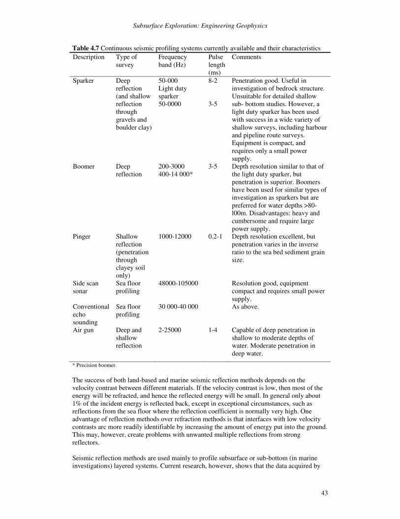
Subsurface Exploration: Engineering Geophysics
43
Table 4.7 Continuous seismic profiling systems currently available and their characteristics Description Type of
survey Frequency band (Hz)
Pulse length (ms)
Comments
Sparker Deep reflection (and shallow reflection through gravels and boulder clay)
50-000 Light duty sparker 50-0000
8-2 3-5
Penetration good. Useful in investigation of bedrock structure. Unsuitable for detailed shallow sub- bottom studies. However, a light duty sparker has been used with success in a wide variety of shallow surveys, including harbour and pipeline route surveys. Equipment is compact, and requires only a small power supply.
Boomer Deep reflection
200-3000 400-14 000*
3-5 Depth resolution similar to that of the light duty sparker, but penetration is superior. Boomers have been used for similar types of investigation as sparkers but are preferred for water depths >80-l00m. Disadvantages: heavy and cumbersome and require large power supply.
Pinger Shallow reflection (penetration through clayey soil only)
1000-12000 0.2-1 Depth resolution excellent, but penetration varies in the inverse ratio to the sea bed sediment grain size.
Side scan sonar
Sea floor profiling
48000-105000 Resolution good, equipment compact and requires small power supply.
Conventional echo sounding
Sea floor profiling
30 000-40 000 As above.
Air gun Deep and shallow reflection
2-25000 1-4 Capable of deep penetration in shallow to moderate depths of water. Moderate penetration in deep water.
* Precision boomer. The success of both land-based and marine seismic reflection methods depends on the velocity contrast between different materials. If the velocity contrast is low, then most of the energy will be refracted, and hence the reflected energy will be small. In general only about 1% of the incident energy is reflected back, except in exceptional circumstances, such as reflections from the sea floor where the reflection coefficient is normally very high. One advantage of reflection methods over refraction methods is that interfaces with low velocity contrasts arc more readily identifiable by increasing the amount of energy put into the ground. This may, however, create problems with unwanted multiple reflections from strong reflectors. Seismic reflection methods are used mainly to profile subsurface or sub-bottom (in marine investigations) layered systems. Current research, however, shows that the data acquired by
Site Investigation
44
such methods are capable of a more detailed interpretation to obtain geotechnical parameters. McCann and Taylor-Smith (1973) review the application of seismic reflection together with other geophysical techniques in the determination of geotechnical parameters of sea-floor sediments. Seismic tomography Tomography (from the Greek, tomos: a slice or section) is a method whereby an image of the distribution of a physical property within an enclosed region is produced without direct access to the zone. Seismic velocity tomography is a geophysical sectioning technique which determines the spatial seismic velocity distribution within a given area of interest. Seismic velocity tomography is potentially extremely useful in geotechnical ground investigations, for two reasons. First, tomography can give information on the general variability (i.e. of seismic velocity) beneath a site, and by inference allow a qualitative assessment of the variability of properties such as stiffness and strength. Features such as voids, fractures, rock layers and soft spots are often difficult to detect using more conventional (boring and drilling) techniques, because only a minute proportion of the sub-soil is sampled and tested by direct methods of ground investigation. Geophysical techniques may be helpful in detecting such features. Secondly, the technique can be used to provide values of the ‘very small strain’ stiffness (Go, or Gmax) of the ground, since this is uniquely linked to seismic shear wave velocity (Vs) through the equation:
ρ2sVG =
� (4.10)
where � = bulk density of the soil. Depending upon the ground conditions and the strain levels imposed by construction, this stiffness may be more or less relevant to the operational stiffness required for the analysis of geotechnical displacement problems. In many ground conditions (for example fractured rock or granular soils) the alternative methods of estimating stiffness may be sufficiently expensive or inaccurate as to make seismic methods attractive. The form of tomography that is, perhaps, most familiar is the technique of computer assisted tomography (CAT), as used in diagnostic medicine. The method of seismic tomography has been in use for some years: amongst the first applications of geotomography was a survey by Bois et al. (1971) in an oil field. In seismic velocity tomography, an image of the distribution of the seismic propagation velocity properties within a region of the ground is deduced from measurements of the transit times of artificially induced seismic waves crossing the zone. The process can be divided into a number of activities, each of which requires careful attention if useful results are to be achieved:
• data acquisition and reduction; • reconstruction of velocities; and • interpretation.
The field geophysical method involves the input of seismic energy (from mechanical hammers, or sparkers) at discrete points down boreholes, and possibly along the ground surface, and the acquisition of seismic records of the incoming wave energy (via geophones or hydrophones) at as many other discrete points around the area of interest as is feasible. The seismic traces are then inspected to determine the first arrival of the wave type of interest. In many rock investigations this may be the onset of primary, compressional (P) waves, but in weaker sediments such as saturated soils, it may be necessary to determine the arrival time of secondary, shear (S) waves. The data required from the field, before reconstruction processing can commence, are the travel times from each source to every receiver, and the co-ordinates of the source and receiver positions.
Subsurface Exploration: Engineering Geophysics
45
Tomographic reconstruction (as applied here) is the mathematical process by which velocities at different points within the ground are calculated. The principles of tomographic reconstruction are well-established (Radon 1917). In general, the region to be imaged is divided into discrete rectangular areas or cells (Fig. 4.25). Let �j be the seismic propagation velocity within the jth of n reconstruction cells. This velocity value applies uniformly across the full area of the cell. The travel time, ti for the ith ray across the grid of cells is given by:
=
��
�
�
��
�
�=
n
j j
iji v
dt
1
(4.11)
where dij = length of the ith ray within the jth cell. In a survey which incorporates m travel times, acquired for rays at various positions and orientations across the region, there will be m such summations. These can be expressed in matrix form as:
Dwt = (4.12) where D is an m × n array having elements of the form dij; w is an n-element column vector containing the current estimate of the reciprocal velocities (‘slownesses’); and t is a column vector of the m travel times calculated across the discretized velocity field. Let p be the column vector of the m observed travel times from a field survey. For reasons to be discussed in detail later, it is usually not possible to find a velocity field which is exactly consistent with the measured travel times. Thus the process of reconstructing a velocity field is equivalent to the minimization of a residual vector, e, defined by the equation:
Dwpe −= (4.13) Commonly used strategies for computerized geotomographic reconstruction include the damped least squares method (Bois et at. 1971), the Back Projection Technique, BPT (Kuhl and Edwards 1963; Neumann-Denzau 1984), the Algebraic Reconstruction Technique, ART (Kaczmarz 1934; Peterson et al. 1985), and the Simultaneous Iterative Reconstruction Technique, SIRT (Dines and Lytle 1979; Gilbert 1972), although many others are available (for example, Gordon and Herman (1974)). The acquisition diagram in Fig. 4.25 shows straight rays. In practice, rays may deviate from straight paths as waves undergo, for example, refraction in an heterogeneous velocity field. Therefore the path followed by a ray, between a source and receiver, is not known. D is a function of w: the elements of w and D are unknown. Thus reconstruction involves not only the distribution of errors along ray paths, but also the determination of an appropriate position for that ray path. The product of reconstruction is a single velocity for each cell. These velocities may be contoured and displayed as colour or grey scales in a tomogram. A seismic velocity tomogram is, necessarily, an approximation. It is a two-dimensional, discrete estimate of a continuously varying, three-dimensional function — that is, the distribution of the seismic velocity properties of the ground. The accuracy of a tomographic estimate of the subsurface and, hence, its usefulness as a predictive tool is influenced by many diverse factors. These affect the ability of the technique to determine the size, form and seismic velocity (and hence stiffness) of features in the ground. Idealizations of wave behaviour Seismic energy travels through the ground as waves. There are a number of different physical theories associated with the description of wave behaviour. Each particular theory or idealization may be useful in one context, but it is often necessary to appeal to more than one theory to understand fully how seismic energy can be transmitted through the ground. For example, a source of seismic energy at a point in a homogeneous isotropic medium will produce a set of spherical wavefronts and these can, as a simplification, be represented as a set of rays emanating from the source (Fig. 4.26a). The ray approximation is convenient for
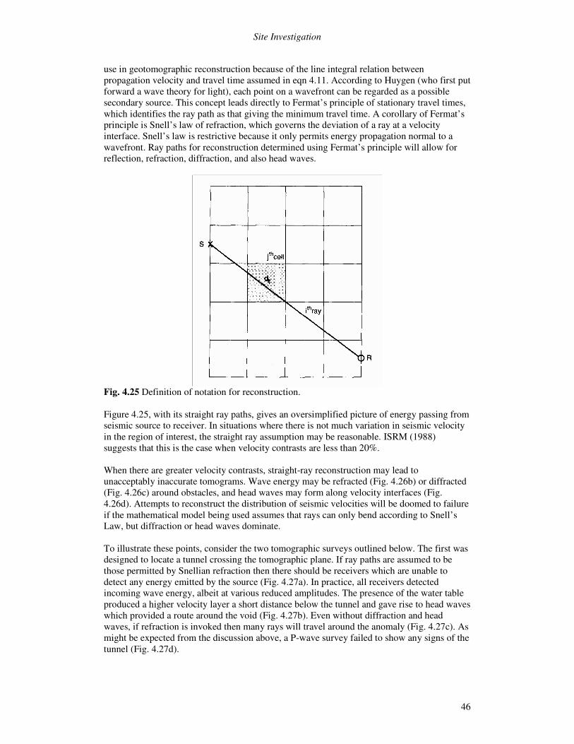
Site Investigation
46
use in geotomographic reconstruction because of the line integral relation between propagation velocity and travel time assumed in eqn 4.11. According to Huygen (who first put forward a wave theory for light), each point on a wavefront can be regarded as a possible secondary source. This concept leads directly to Fermat’s principle of stationary travel times, which identifies the ray path as that giving the minimum travel time. A corollary of Fermat’s principle is Snell’s law of refraction, which governs the deviation of a ray at a velocity interface. Snell’s law is restrictive because it only permits energy propagation normal to a wavefront. Ray paths for reconstruction determined using Fermat’s principle will allow for reflection, refraction, diffraction, and also head waves.
Fig. 4.25 Definition of notation for reconstruction. Figure 4.25, with its straight ray paths, gives an oversimplified picture of energy passing from seismic source to receiver. In situations where there is not much variation in seismic velocity in the region of interest, the straight ray assumption may be reasonable. ISRM (1988) suggests that this is the case when velocity contrasts are less than 20%. When there are greater velocity contrasts, straight-ray reconstruction may lead to unacceptably inaccurate tomograms. Wave energy may be refracted (Fig. 4.26b) or diffracted (Fig. 4.26c) around obstacles, and head waves may form along velocity interfaces (Fig. 4.26d). Attempts to reconstruct the distribution of seismic velocities will be doomed to failure if the mathematical model being used assumes that rays can only bend according to Snell’s Law, but diffraction or head waves dominate. To illustrate these points, consider the two tomographic surveys outlined below. The first was designed to locate a tunnel crossing the tomographic plane. If ray paths are assumed to be those permitted by Snellian refraction then there should be receivers which are unable to detect any energy emitted by the source (Fig. 4.27a). In practice, all receivers detected incoming wave energy, albeit at various reduced amplitudes. The presence of the water table produced a higher velocity layer a short distance below the tunnel and gave rise to head waves which provided a route around the void (Fig. 4.27b). Even without diffraction and head waves, if refraction is invoked then many rays will travel around the anomaly (Fig. 4.27c). As might be expected from the discussion above, a P-wave survey failed to show any signs of the tunnel (Fig. 4.27d).
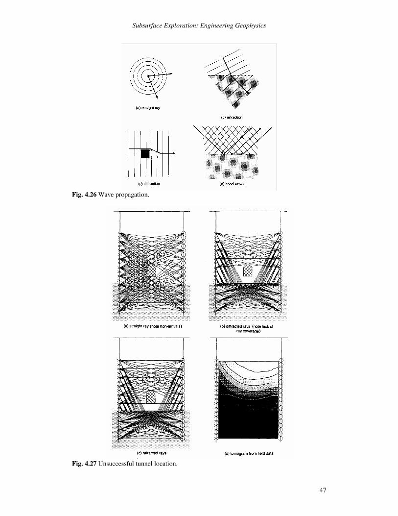
Subsurface Exploration: Engineering Geophysics
47
Fig. 4.26 Wave propagation.
Fig. 4.27 Unsuccessful tunnel location.
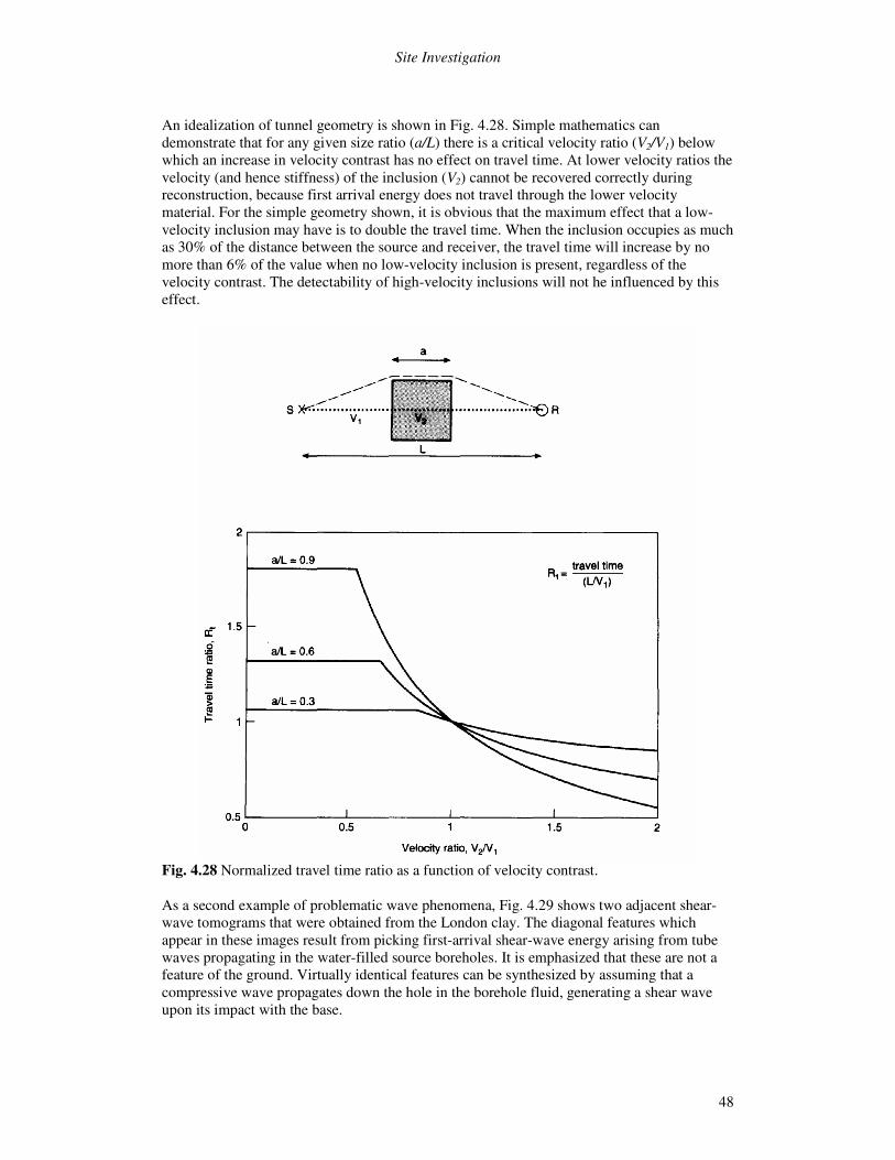
Site Investigation
48
An idealization of tunnel geometry is shown in Fig. 4.28. Simple mathematics can demonstrate that for any given size ratio (a/L) there is a critical velocity ratio (V2/V1) below which an increase in velocity contrast has no effect on travel time. At lower velocity ratios the velocity (and hence stiffness) of the inclusion (V2) cannot be recovered correctly during reconstruction, because first arrival energy does not travel through the lower velocity material. For the simple geometry shown, it is obvious that the maximum effect that a low-velocity inclusion may have is to double the travel time. When the inclusion occupies as much as 30% of the distance between the source and receiver, the travel time will increase by no more than 6% of the value when no low-velocity inclusion is present, regardless of the velocity contrast. The detectability of high-velocity inclusions will not he influenced by this effect.
Fig. 4.28 Normalized travel time ratio as a function of velocity contrast. As a second example of problematic wave phenomena, Fig. 4.29 shows two adjacent shear-wave tomograms that were obtained from the London clay. The diagonal features which appear in these images result from picking first-arrival shear-wave energy arising from tube waves propagating in the water-filled source boreholes. It is emphasized that these are not a feature of the ground. Virtually identical features can be synthesized by assuming that a compressive wave propagates down the hole in the borehole fluid, generating a shear wave upon its impact with the base.
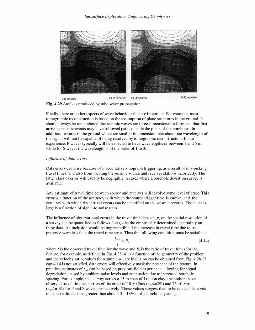
Subsurface Exploration: Engineering Geophysics
49
Fig. 4.29 Atefacts produced by tube-wave propagation. Finally, there are other aspects of wave behaviour that are important. For example, most tomographic reconstruction is based on the assumption of plane structures in the ground. It should always be remembered that seismic waves are three-dimensional in form and that first arriving seismic events may have followed paths outside the plane of the boreholes. In addition, features in the ground which are smaller in dimension than about one wavelength of the signal will not be capable of being resolved by tomographic reconstruction. In our experience, P waves typically will be expected to have wavelengths of between 1 and 5 m, while for S waves the wavelength is of the order of 1 to 3m. Influence of data errors Data errors can arise because of inaccurate seismograph triggering, as a result of mis-picking travel times, and also from locating the seismic source and receiver stations incorrectly. The latter class of error will usually be negligible in cases where a borehole deviation survey is available. Any estimate of travel time between source and receiver will involve some level of error. This error is a function of the accuracy with which the source trigger time is known, and. the certainty with which first arrival events can be identified on the seismic records. The latter is largely a function of signal-to-noise ratio. The influence of observational errors in the travel time data set, p, on the spatial resolution of a survey can be quantified as follows. Let terr be the empirically determined uncertainty on these data. An inclusion would be imperceptible if the increase in travel time due to its presence were less than the travel time error. Thus the following condition must be satisfied:
terr Rt
t< (4.14)
where t is the observed travel time for the wave and Rt is the ratio of travel times for the feature, for example, as defined in Fig. 4.28. Rt is a function of the geometry of the problem and the velocity ratio; values for a simple square inclusion can be obtained from Fig. 4.28. If eqn 4.14 is not satisfied, data errors will effectively mask the presence of the feature. In practice, estimates of terr can be based on previous field experience, allowing for signal degradation caused by ambient noise levels and attenuation due to increased borehole spacing. For example, in a survey across a 15 m span of London clay, the authors have observed travel time and errors of the order of 10 ±0.2ms (terr/t=2%) and 75 ±0.8ms (terr/t=1%) for P and S waves, respectively. These values suggest that, to be detectable, a void must have dimensions greater than about 13—18% of the borehole spacing.
Site Investigation
50
As has been indicated, in a typical geotomographic survey, the matrix D does not have full rank. Furthermore, D is ill-conditioned. Ill-conditioned systems tend to magnify the effects of data errors (Jackson 1972). This problem can be reduced by identifying and excluding outliers from the data set and also by ‘damping out’ the influence of the smaller eigenvalues in the tomographic system. Nevertheless, to some degree, observational errors will, unavoidably, affect a tomogram that is derived from field data. An effective empirical method of assessing the influence of travel time errors on a reconstructed image is given by the following procedure. A numerical model of the suspected velocity field is simulated. Using a suitable ray-tracing algorithm, a set of travel times for theoretical rays across the field are calculated. A second data set is generated by adding random ‘error’ values, limited in magnitude by terr, to the travel times in the first set. Tomograms are reconstructed from both data sets. Subtracting, cell by cell, the reconstructed velocity values in each image will result in a ‘difference’ tomogram. This image indicates the effect of data errors in a particular tomographic system, as processed by the chosen reconstruction algorithm. The image can be interpreted thus: if cell velocities in the difference tomogram show a deviation of, say, 5% from the velocities within adjacent cells, then such fluctuations in a field tomogram should, perhaps, be attributed to observational error rather than genuine variations in the properties of the surveyed region. As with many new and complex techniques, there is a danger that tomography will become discredited as a result of thoughtless misuse. As we have demonstrated above, there are potentially many reasons why the technique might be expected not to succeed, given particular site conditions. If tomography is to be successful then a number of basic criteria should be applied during the planning and design of the work. The preliminary design of a tomographic survey should consider:
1. the type of wave to be used (i.e. P or S). This decision should be made on the basis of the expected velocity contrasts in each case, and the predicted wavelength in relation to any target;
2. the expected signal-to-noise ratio, and the repeatability with which the seismograph can be triggered by the source; these will influence the travel time errors; and
3. the size and geometry of the required tomogram, based on the amount of ground to be investigated, and the expected size of the target.
It is essential that shallow tomographic surveys are planned on the basis of a reasonable knowledge of the likely range of ground stiffnesses (and hence seismic velocities), and the information required from the survey. If tomography is intended to detect a ‘target’ (for example, a fault or a cavity) then the possible orientations and sizes of the target should be estimated. Following this, synthetic travel times should be generated for a number of possible survey geometries (i.e. borehole separation, and the down-hole source and receiver spacings) and processed using a range of reconstruction techniques. In this way, the design of the survey may be optimized and the viability of the technique assessed. On the basis of our experience to date, the following may be stated.
1. Low-velocity anomalies (such as cavities) appear more difficult to detect than high-velocity anomalies (for example, hard inclusions).
2. The absolute values of seismic velocity recovered from a survey may be regarded as indicative of ground stiffness variations, but should not be used in an absolute way in engineering calculations.
3. Velocity variations are likely to be most reliably reconstructed when velocity contrasts are low.
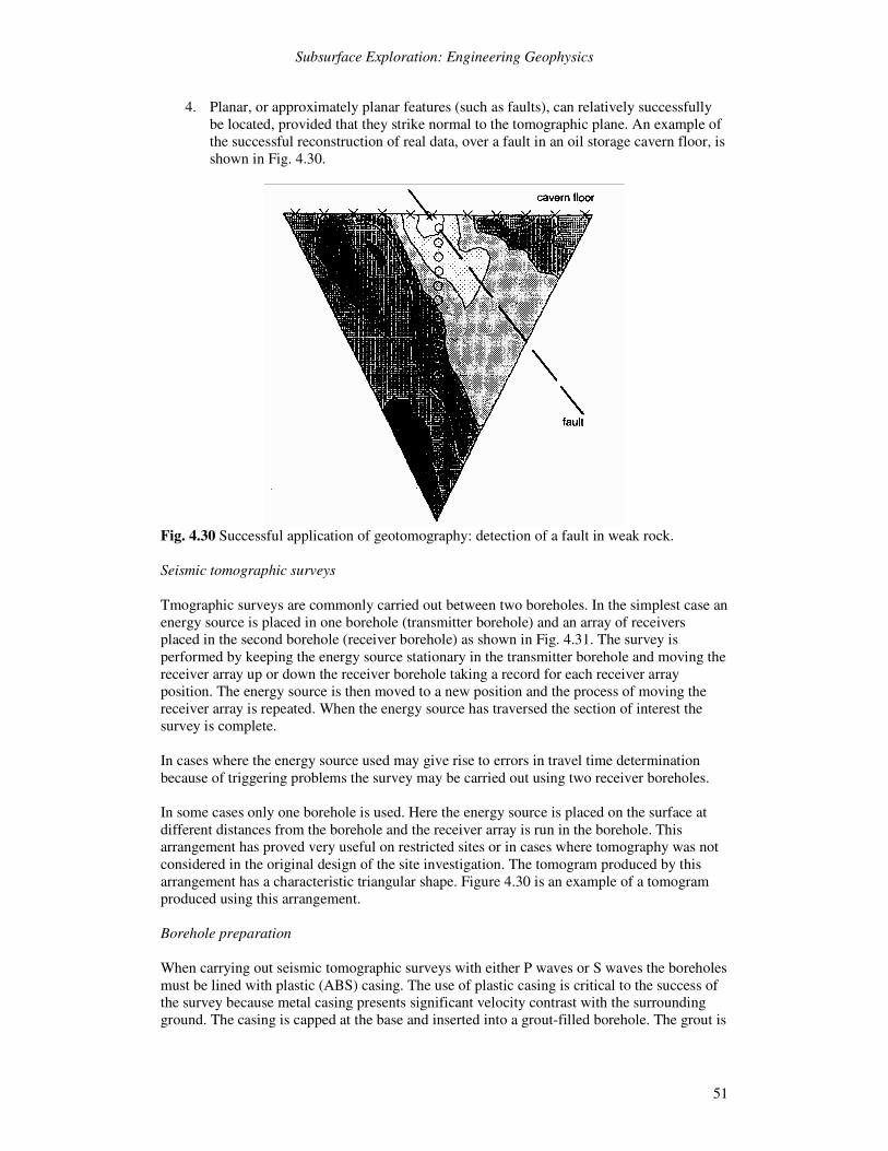
Subsurface Exploration: Engineering Geophysics
51
4. Planar, or approximately planar features (such as faults), can relatively successfully be located, provided that they strike normal to the tomographic plane. An example of the successful reconstruction of real data, over a fault in an oil storage cavern floor, is shown in Fig. 4.30.
Fig. 4.30 Successful application of geotomography: detection of a fault in weak rock. Seismic tomographic surveys Tmographic surveys are commonly carried out between two boreholes. In the simplest case an energy source is placed in one borehole (transmitter borehole) and an array of receivers placed in the second borehole (receiver borehole) as shown in Fig. 4.31. The survey is performed by keeping the energy source stationary in the transmitter borehole and moving the receiver array up or down the receiver borehole taking a record for each receiver array position. The energy source is then moved to a new position and the process of moving the receiver array is repeated. When the energy source has traversed the section of interest the survey is complete. In cases where the energy source used may give rise to errors in travel time determination because of triggering problems the survey may be carried out using two receiver boreholes. In some cases only one borehole is used. Here the energy source is placed on the surface at different distances from the borehole and the receiver array is run in the borehole. This arrangement has proved very useful on restricted sites or in cases where tomography was not considered in the original design of the site investigation. The tomogram produced by this arrangement has a characteristic triangular shape. Figure 4.30 is an example of a tomogram produced using this arrangement. Borehole preparation When carrying out seismic tomographic surveys with either P waves or S waves the boreholes must be lined with plastic (ABS) casing. The use of plastic casing is critical to the success of the survey because metal casing presents significant velocity contrast with the surrounding ground. The casing is capped at the base and inserted into a grout-filled borehole. The grout is
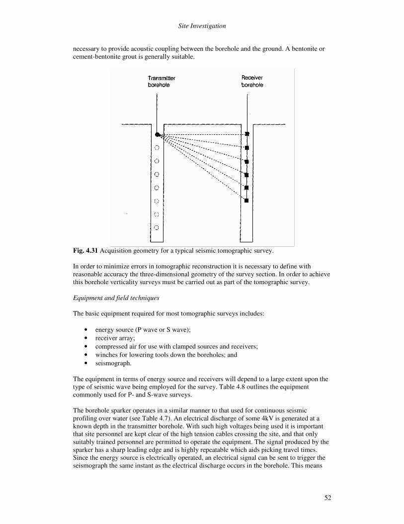
Site Investigation
52
necessary to provide acoustic coupling between the borehole and the ground. A bentonite or cement-bentonite grout is generally suitable.
Fig. 4.31 Acquisition geometry for a typical seismic tomographic survey. In order to minimize errors in tomographic reconstruction it is necessary to define with reasonable accuracy the three-dimensional geometry of the survey section. In order to achieve this borehole verticality surveys must be carried out as part of the tomographic survey. Equipment and field techniques The basic equipment required for most tomographic surveys includes:
• energy source (P wave or S wave); • receiver array; • compressed air for use with clamped sources and receivers; • winches for lowering tools down the boreholes; and • seismograph.
The equipment in terms of energy source and receivers will depend to a large extent upon the type of seismic wave being employed for the survey. Table 4.8 outlines the equipment commonly used for P- and S-wave surveys. The borehole sparker operates in a similar manner to that used for continuous seismic profiling over water (see Table 4.7). An electrical discharge of some 4kV is generated at a known depth in the transmitter borehole. With such high voltages being used it is important that site personnel are kept clear of the high tension cables crossing the site, and that only suitably trained personnel are permitted to operate the equipment. The signal produced by the sparker has a sharp leading edge and is highly repeatable which aids picking travel times. Since the energy source is electrically operated, an electrical signal can be sent to trigger the seismograph the same instant as the electrical discharge occurs in the borehole. This means
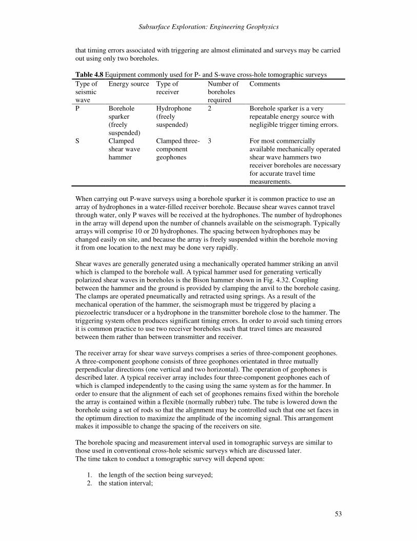
Subsurface Exploration: Engineering Geophysics
53
that timing errors associated with triggering are almost eliminated and surveys may be carried out using only two boreholes. Table 4.8 Equipment commonly used for P- and S-wave cross-hole tomographic surveys Type of seismic wave
Energy source Type of receiver
Number of boreholes required
Comments
P Borehole sparker (freely suspended)
Hydrophone (freely suspended)
2 Borehole sparker is a very repeatable energy source with negligible trigger timing errors.
S Clamped shear wave hammer
Clamped three- component geophones
3 For most commercially available mechanically operated shear wave hammers two receiver boreholes are necessary for accurate travel time measurements.
When carrying out P-wave surveys using a borehole sparker it is common practice to use an array of hydrophones in a water-filled receiver borehole. Because shear waves cannot travel through water, only P waves will be received at the hydrophones. The number of hydrophones in the array will depend upon the number of channels available on the seismograph. Typically arrays will comprise 10 or 20 hydrophones. The spacing between hydrophones may be changed easily on site, and because the array is freely suspended within the borehole moving it from one location to the next may be done very rapidly. Shear waves are generally generated using a mechanically operated hammer striking an anvil which is clamped to the borehole wall. A typical hammer used for generating vertically polarized shear waves in boreholes is the Bison hammer shown in Fig. 4.32. Coupling between the hammer and the ground is provided by clamping the anvil to the borehole casing. The clamps are operated pneumatically and retracted using springs. As a result of the mechanical operation of the hammer, the seismograph must be triggered by placing a piezoelectric transducer or a hydrophone in the transmitter borehole close to the hammer. The triggering system often produces significant timing errors. In order to avoid such timing errors it is common practice to use two receiver boreholes such that travel times are measured between them rather than between transmitter and receiver. The receiver array for shear wave surveys comprises a series of three-component geophones. A three-component geophone consists of three geophones orientated in three mutually perpendicular directions (one vertical and two horizontal). The operation of geophones is described later. A typical receiver array includes four three-component geophones each of which is clamped independently to the casing using the same system as for the hammer. In order to ensure that the alignment of each set of geophones remains fixed within the borehole the array is contained within a flexible (normally rubber) tube. The tube is lowered down the borehole using a set of rods so that the alignment may be controlled such that one set faces in the optimum direction to maximize the amplitude of the incoming signal. This arrangement makes it impossible to change the spacing of the receivers on site. The borehole spacing and measurement interval used in tomographic surveys are similar to those used in conventional cross-hole seismic surveys which are discussed later. The time taken to conduct a tomographic survey will depend upon:
1. the length of the section being surveyed; 2. the station interval;
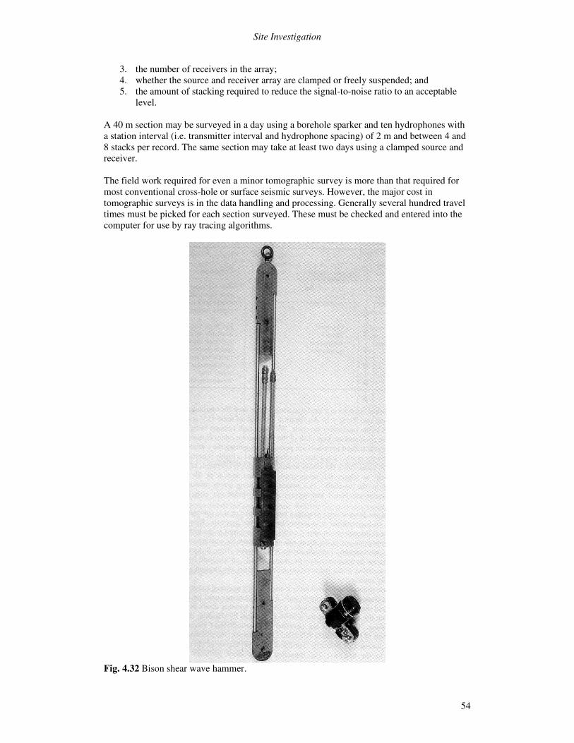
Site Investigation
54
3. the number of receivers in the array; 4. whether the source and receiver array are clamped or freely suspended; and 5. the amount of stacking required to reduce the signal-to-noise ratio to an acceptable
level. A 40 m section may be surveyed in a day using a borehole sparker and ten hydrophones with a station interval (i.e. transmitter interval and hydrophone spacing) of 2 m and between 4 and 8 stacks per record. The same section may take at least two days using a clamped source and receiver. The field work required for even a minor tomographic survey is more than that required for most conventional cross-hole or surface seismic surveys. However, the major cost in tomographic surveys is in the data handling and processing. Generally several hundred travel times must be picked for each section surveyed. These must be checked and entered into the computer for use by ray tracing algorithms.
Fig. 4.32 Bison shear wave hammer.
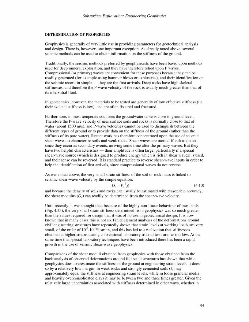
Subsurface Exploration: Engineering Geophysics
55
DETERMINATION OF PROPERTIES Geophysics is generally of very little use in providing parameters for geotechnical analysis and design. There is, however, one important exception. As already noted above, several seismic methods can be used to obtain information on the stiffness of the ground. Traditionally, the seismic methods preferred by geophysicists have been based upon methods used for deep mineral exploration, and they have therefore relied upon P waves. Compressional (or primary) waves are convenient for these purposes because they can be readily generated (for example using hammer blows or explosives), and their identification on the seismic record in simple — they are the first arrivals. Deep rocks have high skeletal stiffnesses, and therefore the P-wave velocity of the rock is usually much greater than that of its interstitial fluid. In geotechnics, however, the materials to be tested are generally of low effective stiffness (i.e. their skeletal stiffness is low), and are often fissured and fractured. Furthermore, in most temperate countries the groundwater table is close to ground level. Therefore the P-wave velocity of near surface soils and rocks is normally close to that of water (about 1500 m/s), and P-wave velocities cannot be used to distinguish between the different types of ground or to provide data on the stiffness of the ground (rather than the stiffness of its pore water). Recent work has therefore concentrated upon the use of seismic shear waves to characterize soils and weak rocks. Shear waves are more difficult to detect, since they occur as secondary events, arriving some time after the primary waves. But they have two helpful characteristics — their amplitude is often large, particularly if a special shear-wave source (which is designed to produce energy which is rich in shear waves) is used, and their sense can be reversed. It is standard practice to reverse shear-wave inputs in order to help the identification of first arrivals, since compressional waves do not reverse. As was noted above, the very small strain stiffness of the soil or rock mass is linked to seismic shear-wave velocity by the simple equation:
ρ2sVG =
� (4.10)
and because the density of soils and rocks can usually be estimated with reasonable accuracy, the shear modulus (Go) can readily be determined from the shear-wave velocity. Until recently, it was thought that, because of the highly non-linear behaviour of most soils (Fig. 4.33), the very small strain stiffness determined from geophysics was so much greater than the values required for design that it was of no use in geotechnical design. It is now known that in many cases this is not so. Finite element analyses of the deformations around civil engineering structures have repeatedly shown that strain levels at working loads are very small, of the order of 10-2-10-1% strain, and this has led to a realization that stiffnesses obtained at higher strains during conventional laboratory triaxial tests are far too low. At the same time that special laboratory techniques have been introduced there has been a rapid growth in the use of seismic shear-wave geophysics. Comparisons of the shear moduli obtained from geophysics with those obtained from the back-analysis of observed deformations around full-scale structures has shown that while geophysics does overestimate the stiffness of the ground at engineering strain levels, it does so by a relatively low margin. In weak rocks and strongly cemented soils Go may approximately equal the stiffness at engineering strain levels, while in loose granular media and heavily overconsolidated clays it may be between two and three times greater. Given the relatively large uncertainties associated with stiffness determined in other ways, whether in
Site Investigation
56
the laboratory or using in situ testing, shear-wave geophysics must be regarded as a very useful site investigation technique.
Fig. 4.33 Stiffness degradation curve for stiff clay from Tokyo Bay (Mukabi et al. 1991). Laboratory measurements of small-strain stiffness have frequently been reported in the literature, and are now commonplace in UK site investigation practice, and there are also well-established more conventional in situ testing techniques which can be used to determine the stiffness of the ground (for example, plate tests and pressuremeter tests), so that it might be thought that there is little point in carrying out further (very small strain) stiffness measurements by geophysics. However, laboratory tests are subject to sample disturbance, and may not be possible in some soils, because sampling is impossible. And both laboratory and in situ tests are generally carried out on small elements of soil, and may not give stiffnesses which are representative of the mass, inclusive of fracturing and the full range of particle sizes present. Below we describe three techniques which are relatively well established, and under normal circumstances (in the absence of severe background noise) can be expected to yield good results.
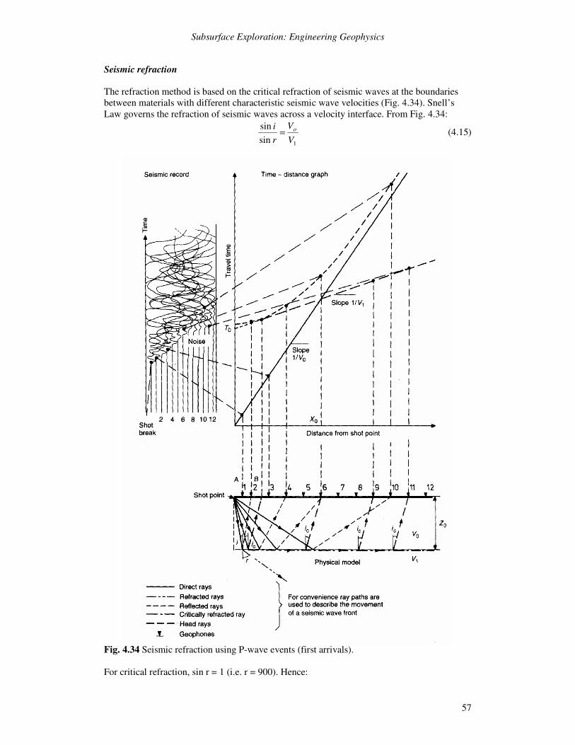
Subsurface Exploration: Engineering Geophysics
57
Seismic refraction The refraction method is based on the critical refraction of seismic waves at the boundaries between materials with different characteristic seismic wave velocities (Fig. 4.34). Snell’s Law governs the refraction of seismic waves across a velocity interface. From Fig. 4.34:
1sinsin
VV
ri o= (4.15)
Fig. 4.34 Seismic refraction using P-wave events (first arrivals). For critical refraction, sin r = 1 (i.e. r = 900). Hence:
Site Investigation
58
1
sinVV
i oc = (4.16)
Critical refraction therefore will only occur if V1> V0, and the rays meet the interface at the critical angle of incidence, ic. If V1 < V0, rays will be refracted towards the normal to the interface making critical refraction impossible. This imposes a limitation on the method and is discussed in more detail later. If a ray meets the interface at an angle less than the critical angle, refraction takes place and the ray continues downwards (Fig. 4.34). Also some of the energy is reflected at the interface. If the angle of incidence exceeds the critical angle, total reflection occurs. The critically refracted ray travels along the interface in the lower (higher velocity) medium. This produces an oscillatory motion parallel to, and immediately below, the interface. Because there is no slippage along the interface, the upper medium is forced to move with the lower medium in a zone adjacent to the interface. This causes the generation of continuous new disturbances which are analogous to sonic booms produced by aircraft flying at supersonic speeds. The shock waves produced are known as head waves. It can be shown that the resultant head wave fronts emerge at the critical angle 4, (Dix 1939). It is the detection of the head wave by the geophones that enables data to be obtained for layers other than the surface layer. The seismic record produced by a geophone placed at a given distance from the energy source will show a combination of direct events,2 refracted events (head waves), reflected events and ‘ground roll’ (surface waves). The reflected waves will always arrive later than the direct waves or the refracted waves. In one special case, the refracted wave and the reflected wave arrive simultaneously. The energy source to geophone distance at which this occurs for a simple two layer case (Fig. 4.34) is given by:
ciZx tan2 0= (4.17) where x = distance between energy source and geophone, Z0 = depth to first refractor and ic = critical angle. At distances less than 2Z0 tan ic the head wave does not exist and hence no refracted events appear on the seismic record. In Fig. 4.34 the geophones nearest the energy source (shot point) will record the direct wave as a first arrival event. However, because the critically refracted wave travels at a greater velocity than the direct wave, eventually the head wave produced at the interface will arrive at the geophones before the direct wave. The distance from the shot point at which the direct wave and the head wave arrive at the ground surface simultaneously is termed the critical distance X0. The critical distance is used in the interpretation of seismic refraction data. Other critical distances may be defined for multilayer systems for the simultaneous arrival of refracted waves from different layers. The equipment required for refraction surveying includes an energy source, geophones, a take-out cable, and a signal-enhancement seismograph. The fundamental requirement for an energy source for seismic surveying is that it should be capable of delivering to the ground an impulse which has a sharp leading edge, so that first-arrival events can be accurately picked from the geophysical records. Traditionally seismic refraction has been used primarily to determine sub-soil geometry, and has used compressional wave arrivals. For this purpose, and for investigation of shallow depths, it has been sufficient to use a sledge hammer striking a metal plate placed on the ground or, for greater depths of penetration, detonators placed in shallow holes. Figure 4.35 contrasts this
2 The signal produced by a geophone in response to a wave front is termed an event.
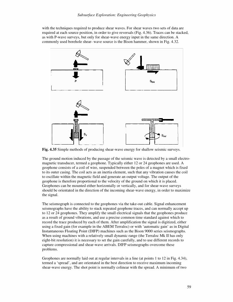
Subsurface Exploration: Engineering Geophysics
59
with the techniques required to produce shear waves. For shear waves two sets of data are required at each source position, in order to give reversals (Fig. 4.36). Traces can be stacked, as with P-wave surveys, but only for shear-wave energy input in the same direction. A commonly used borehole shear- wave source is the Bison hammer, shown in Fig. 4.32.
Fig. 4.35 Simple methods of producing shear-wave energy for shallow seismic surveys. The ground motion induced by the passage of the seismic wave is detected by a small electro-magnetic transducer, termed a geophone. Typically either 12 or 24 geophones are used. A geophone consists of a coil of wire, suspended between the poles of a magnet which is fixed to its outer casing. The coil acts as an inertia element, such that any vibration causes the coil to oscillate within the magnetic field and generate an output voltage. The output of the geophone is therefore proportional to the velocity of the ground on which it is placed. Geophones can be mounted either horizontally or vertically, and for shear-wave surveys should be orientated in the direction of the incoming shear-wave energy, in order to maximize the signal. The seismograph is connected to the geophones via the take-out cable. Signal enhancement seismographs have the ability to stack repeated geophone traces, and can normally accept up to 12 or 24 geophones. They amplify the small electrical signals that the geophones produce as a result of ground vibrations, and use a precise common time standard against which to record the trace produced by each of them. After amplification the signal is digitized, either using a fixed gain (for example in the ABEM Terraloc) or with ‘automatic gain’ as in Digital Instantaneous Floating Point (DIFP) machines such as the Bison 9000 series seismographs. When using machines with a relatively small dynamic range (the Terraloc Mk II has only eight-bit resolution) it is necessary to set the gain carefully, and to use different records to capture compressional and shear-wave arrivals. DIFP seismographs overcome these problems. Geophones are normally laid out at regular intervals in a line (at points 1 to 12 in Fig. 4.34), termed a ‘spread’, and are orientated in the best direction to receive maximum incoming shear-wave energy. The shot point is normally colinear with the spread. A minimum of two
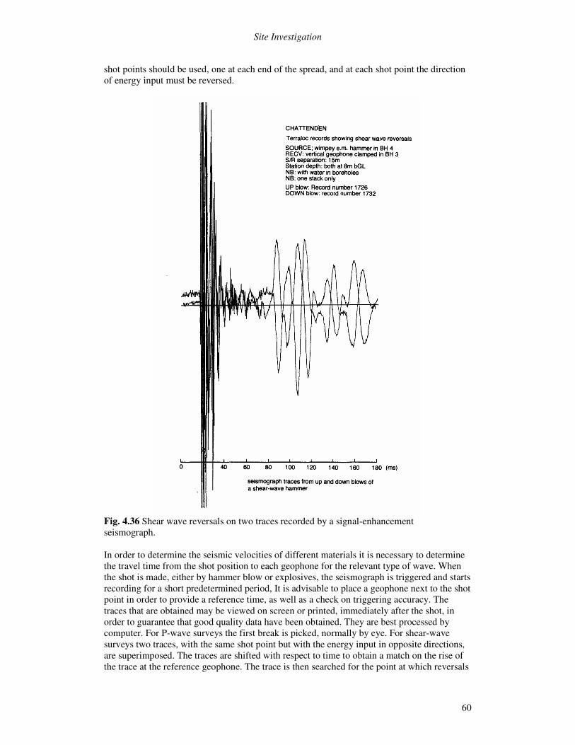
Site Investigation
60
shot points should be used, one at each end of the spread, and at each shot point the direction of energy input must be reversed.
Fig. 4.36 Shear wave reversals on two traces recorded by a signal-enhancement seismograph. In order to determine the seismic velocities of different materials it is necessary to determine the travel time from the shot position to each geophone for the relevant type of wave. When the shot is made, either by hammer blow or explosives, the seismograph is triggered and starts recording for a short predetermined period, It is advisable to place a geophone next to the shot point in order to provide a reference time, as well as a check on triggering accuracy. The traces that are obtained may be viewed on screen or printed, immediately after the shot, in order to guarantee that good quality data have been obtained. They are best processed by computer. For P-wave surveys the first break is picked, normally by eye. For shear-wave surveys two traces, with the same shot point but with the energy input in opposite directions, are superimposed. The traces are shifted with respect to time to obtain a match on the rise of the trace at the reference geophone. The trace is then searched for the point at which reversals
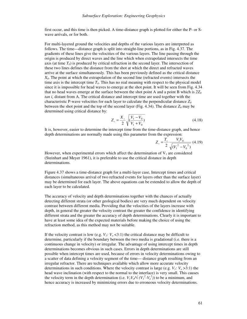
Subsurface Exploration: Engineering Geophysics
61
first occur, and this time is then picked. A time-distance graph is plotted for either the P- or S-wave arrivals, or for both. For multi-layered ground the velocities and depths of the various layers are interpreted as follows. The time—distance graph is split into straight-line portions, as in Fig. 4.37. The gradients of these lines give the velocities of the various layers. The line passing through the origin is produced by direct waves and the line which when extrapolated intersects the time axis (at time T0) is produced by critical refraction in the second layer. The intersection of these two lines defines the distance from the shot at which the direct and refracted waves arrive at the surface simultaneously. This has been previously defined as the critical distance X0. The point at which the extrapolation of the second line (refracted events) intersects the time axis is the intercept time T0. This has no real meaning with respect to the physical model since it is impossible for head waves to emerge at the shot point. It will be seen from Fig. 4.34 that no head waves emerge at the surface between the shot point A and a point B which is 2Z0 tan ic distant from A. The critical distance and intercept time are used together with the characteristic P-wave velocities for each layer to calculate the perpendicular distance Z0 between the shot point and the top of the second layer (Fig. 4.34). The distance Z0 may be determined using critical distance by:
)(2 01
01
VVVVX
Z+−
= �
� (4.18)
It is, however, easier to determine the intercept time from the time-distance graph, and hence depth determinations are normally made using this parameter from the expression:
)(2 2
02
1
01
VV
VVTZ
−= �
�(4.19)
However, when experimental errors which affect the determination of V1 are considered (Steinhart and Meyer 1961), it is preferable to use the critical distance in depth determinations. Figure 4.37 shows a time-distance graph for a multi-layer case, Intercept times and critical distances (simultaneous arrival of two refracted events for layers other than the surface layer) may be determined for each layer. The above equations can be extended to allow the depth of each layer to be calculated. The accuracy of velocity and depth determinations together with the chances of actually detecting different strata (or other geological bodies) are very much dependent on velocity contrast between different media. Providing that the velocities of the layers increase with depth, in general the greater the velocity contrast the greater the confidence in identifying different strata and the greater the accuracy of depth determinations. Clearly it is important to have at least some idea of the expected materials before making the choice of using the refraction method, as this method may not be suitable. If the velocity contrast is low (e.g. V1: Vo <3:1) the critical distance may be difficult to determine, particularly if the boundary between the two media is gradational (i.e. there is a continuous change in velocity) or irregular. The advantage of using intercept times in depth determinations becomes obvious in such cases. Errors in depth determinations are still possible when intercept times are used, because of errors in velocity determinations owing to a scatter of data defining a velocity segment of the time— distance graph resulting from an irregular refractor. There are techniques available which allow more accurate velocity determinations in such conditions. Where the velocity contrast is large (e.g. V1: Vo >3:1) the head wave inclination (with respect to the normal to the interface) is very small. This causes the velocity term in the depth determination (i.e. V1Vo/� (V1
2-Vo2)) to be a minimum, and
hence accuracy is increased by minimizing errors due to erroneous velocity determinations.
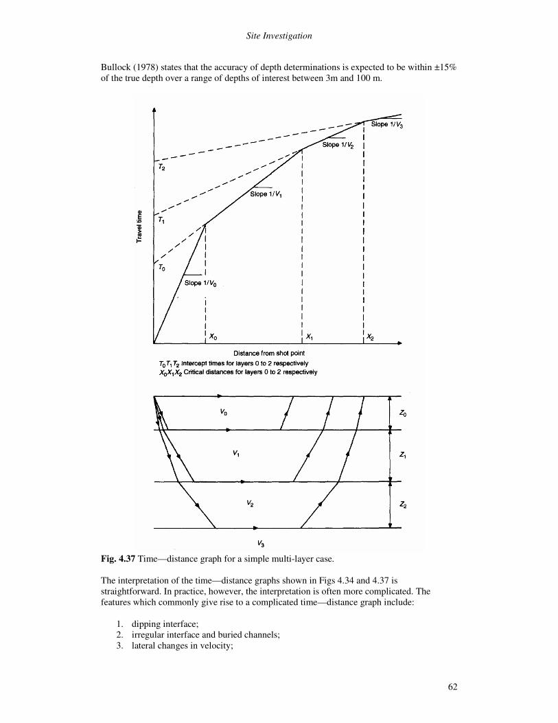
Site Investigation
62
Bullock (1978) states that the accuracy of depth determinations is expected to be within ±15% of the true depth over a range of depths of interest between 3m and 100 m.
Fig. 4.37 Time—distance graph for a simple multi-layer case. The interpretation of the time—distance graphs shown in Figs 4.34 and 4.37 is straightforward. In practice, however, the interpretation is often more complicated. The features which commonly give rise to a complicated time—distance graph include:
1. dipping interface; 2. irregular interface and buried channels; 3. lateral changes in velocity;
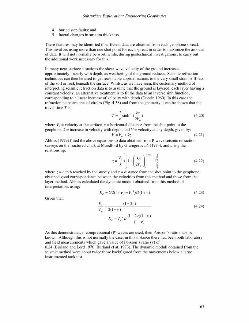
Subsurface Exploration: Engineering Geophysics
63
4. buried step faults; and 5. lateral changes in stratum thickness.
These features may be identified if sufficient data are obtained from each geophone spread. This involves using more than one shot point for each spread in order to maximize the amount of data. It will not normally be worthwhile, during geotechnical investigations, to carry out the additional work necessary for this. In many near-surface situations the shear-wave velocity of the ground increases approximately linearly with depth, as weathering of the ground reduces. Seismic refraction techniques can then be used to get reasonable approximations to the very small strain stiffness of the soil or rock beneath the surface. Whilst, as we have seen, the customary method of interpreting seismic refraction data is to assume that the ground is layered, each layer having a constant velocity, an alternative treatment is to fit the data to an inverse sinh function, corresponding to a linear increase of velocity with depth (Dobrin 1960). In this case the refraction paths are arcs of circles (Fig. 4.38) and from the geometry it can be shown that the travel time T is:
)2
(sinh2 1
oVkx
kT −= (4.20)
where V0 = velocity at the surface, x = horizontal distance from the shot point to the geophone, k = increase in velocity with depth, and V = velocity at any depth, given by:
kzVV o += (4.21) Abbiss (1979) fitted the above equations to data obtained from P-wave seismic refraction surveys on the fractured chalk at Mundford by Grainger et al. (1973), and using the relationship:
��
��
�
��
��
�−
���
�
����
����
�+= 1
21
2/1
o
o
Vkx
kV
z (4.22)
where z = depth reached by the survey and x = distance from the shot point to the geophone, obtained good correspondence between the velocities from this method and those from the layer method. Abbiss calculated the dynamic moduli obtained from this method of interpretation, using:
)1(2)1(2 2 νρν +=+= sd VGE (4.23) Given that:
)1()1)(21(
)1(2)21(
2
νννρ
νν
−+−=
−−=
pd
p
s
VE
VV
(4.24)
As this demonstrates, if compressional (P) waves are used, then Poisson’s ratio must be known. Although this is not normally the case, in this instance there had been both laboratory and field measurements which gave a value of Poisson’s ratio (v) of 0.24 (Burland and Lord 1970; Burland et at. 1973). The dynamic moduli obtained from the seismic method were about twice those backfigured from the movements below a large instrumented tank test.
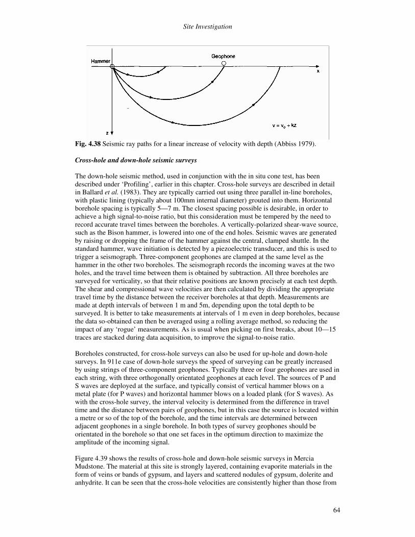
Site Investigation
64
Fig. 4.38 Seismic ray paths for a linear increase of velocity with depth (Abbiss 1979). Cross-hole and down-hole seismic surveys The down-hole seismic method, used in conjunction with the in situ cone test, has been described under ‘Profiling’, earlier in this chapter. Cross-hole surveys are described in detail in Ballard et al. (1983). They are typically carried out using three parallel in-line boreholes, with plastic lining (typically about 100mm internal diameter) grouted into them. Horizontal borehole spacing is typically 5—7 m. The closest spacing possible is desirable, in order to achieve a high signal-to-noise ratio, but this consideration must be tempered by the need to record accurate travel times between the boreholes. A vertically-polarized shear-wave source, such as the Bison hammer, is lowered into one of the end holes. Seismic waves are generated by raising or dropping the frame of the hammer against the central, clamped shuttle. In the standard hammer, wave initiation is detected by a piezoelectric transducer, and this is used to trigger a seismograph. Three-component geophones are clamped at the same level as the hammer in the other two boreholes. The seismograph records the incoming waves at the two holes, and the travel time between them is obtained by subtraction. All three boreholes are surveyed for verticality, so that their relative positions are known precisely at each test depth. The shear and compressional wave velocities are then calculated by dividing the appropriate travel time by the distance between the receiver boreholes at that depth. Measurements are made at depth intervals of between 1 m and 5m, depending upon the total depth to be surveyed. It is better to take measurements at intervals of 1 m even in deep boreholes, because the data so-obtained can then be averaged using a rolling average method, so reducing the impact of any ‘rogue’ measurements. As is usual when picking on first breaks, about 10—15 traces are stacked during data acquisition, to improve the signal-to-noise ratio. Boreholes constructed, for cross-hole surveys can also be used for up-hole and down-hole surveys. In 911e case of down-hole surveys the speed of surveying can be greatly increased by using strings of three-component geophones. Typically three or four geophones are used in each string, with three orthogonally orientated geophones at each level. The sources of P and S waves are deployed at the surface, and typically consist of vertical hammer blows on a metal plate (for P waves) and horizontal hammer blows on a loaded plank (for S waves). As with the cross-hole survey, the interval velocity is determined from the difference in travel time and the distance between pairs of geophones, but in this case the source is located within a metre or so of the top of the borehole, and the time intervals are determined between adjacent geophones in a single borehole. In both types of survey geophones should be orientated in the borehole so that one set faces in the optimum direction to maximize the amplitude of the incoming signal. Figure 4.39 shows the results of cross-hole and down-hole seismic surveys in Mercia Mudstone. The material at this site is strongly layered, containing evaporite materials in the form of veins or bands of gypsum, and layers and scattered nodules of gypsum, dolerite and anhydrite. It can be seen that the cross-hole velocities are consistently higher than those from
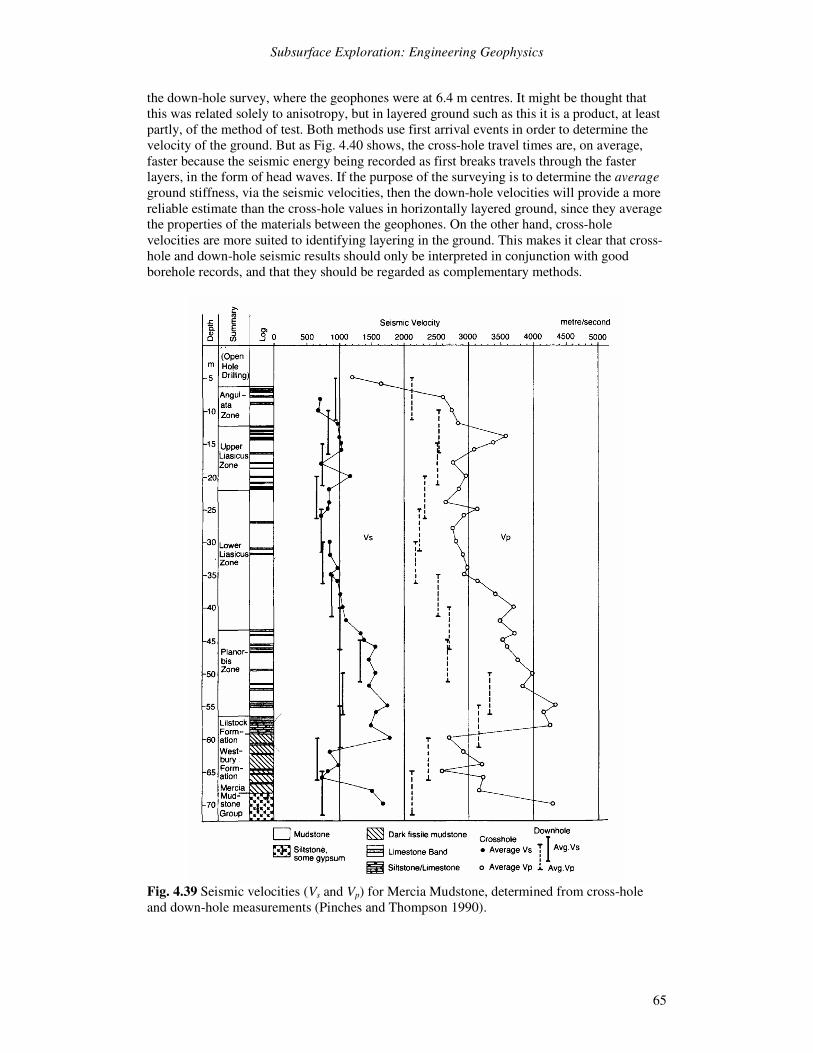
Subsurface Exploration: Engineering Geophysics
65
the down-hole survey, where the geophones were at 6.4 m centres. It might be thought that this was related solely to anisotropy, but in layered ground such as this it is a product, at least partly, of the method of test. Both methods use first arrival events in order to determine the velocity of the ground. But as Fig. 4.40 shows, the cross-hole travel times are, on average, faster because the seismic energy being recorded as first breaks travels through the faster layers, in the form of head waves. If the purpose of the surveying is to determine the average ground stiffness, via the seismic velocities, then the down-hole velocities will provide a more reliable estimate than the cross-hole values in horizontally layered ground, since they average the properties of the materials between the geophones. On the other hand, cross-hole velocities are more suited to identifying layering in the ground. This makes it clear that cross-hole and down-hole seismic results should only be interpreted in conjunction with good borehole records, and that they should be regarded as complementary methods.
Fig. 4.39 Seismic velocities (Vs and Vp) for Mercia Mudstone, determined from cross-hole and down-hole measurements (Pinches and Thompson 1990).
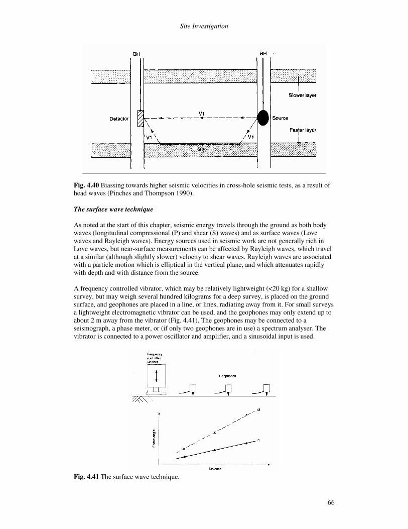
Site Investigation
66
Fig. 4.40 Biassing towards higher seismic velocities in cross-hole seismic tests, as a result of head waves (Pinches and Thompson 1990). The surface wave technique As noted at the start of this chapter, seismic energy travels through the ground as both body waves (longitudinal compressional (P) and shear (S) waves) and as surface waves (Love waves and Rayleigh waves). Energy sources used in seismic work are not generally rich in Love waves, but near-surface measurements can be affected by Rayleigh waves, which travel at a similar (although slightly slower) velocity to shear waves. Rayleigh waves are associated with a particle motion which is elliptical in the vertical plane, and which attenuates rapidly with depth and with distance from the source. A frequency controlled vibrator, which may be relatively lightweight (<20 kg) for a shallow survey, but may weigh several hundred kilograms for a deep survey, is placed on the ground surface, and geophones are placed in a line, or lines, radiating away from it. For small surveys a lightweight electromagnetic vibrator can be used, and the geophones may only extend up to about 2 m away from the vibrator (Fig. 4.41). The geophones may be connected to a seismograph, a phase meter, or (if only two geophones are in use) a spectrum analyser. The vibrator is connected to a power oscillator and amplifier, and a sinusoidal input is used.
Fig. 4.41 The surface wave technique.
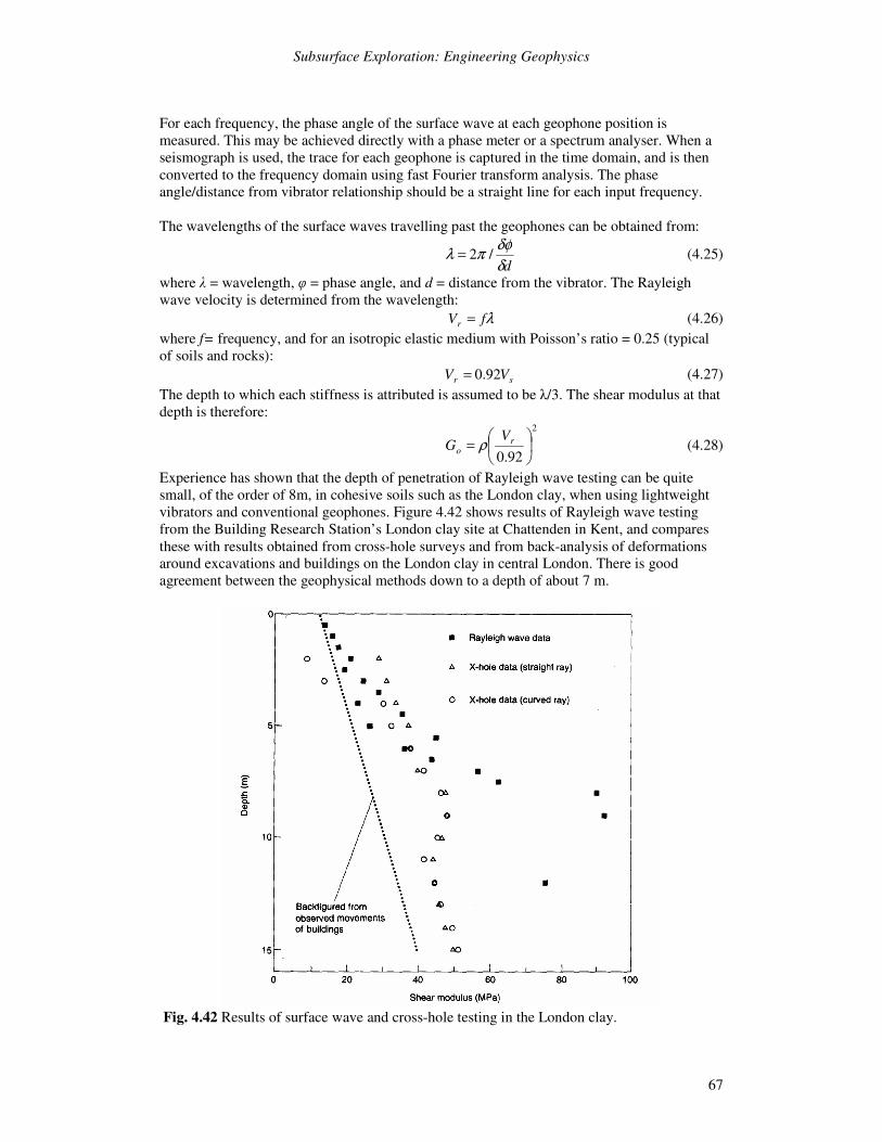
Subsurface Exploration: Engineering Geophysics
67
For each frequency, the phase angle of the surface wave at each geophone position is measured. This may be achieved directly with a phase meter or a spectrum analyser. When a seismograph is used, the trace for each geophone is captured in the time domain, and is then converted to the frequency domain using fast Fourier transform analysis. The phase angle/distance from vibrator relationship should be a straight line for each input frequency. The wavelengths of the surface waves travelling past the geophones can be obtained from:
dδδφπλ /2= (4.25)
where � = wavelength, � = phase angle, and d = distance from the vibrator. The Rayleigh wave velocity is determined from the wavelength:
λfVr = (4.26) where f= frequency, and for an isotropic elastic medium with Poisson’s ratio = 0.25 (typical of soils and rocks):
sr VV 92.0= (4.27) The depth to which each stiffness is attributed is assumed to be �/3. The shear modulus at that depth is therefore:
2
92.0��
���
�= ro
VG ρ (4.28)
Experience has shown that the depth of penetration of Rayleigh wave testing can be quite small, of the order of 8m, in cohesive soils such as the London clay, when using lightweight vibrators and conventional geophones. Figure 4.42 shows results of Rayleigh wave testing from the Building Research Station’s London clay site at Chattenden in Kent, and compares these with results obtained from cross-hole surveys and from back-analysis of deformations around excavations and buildings on the London clay in central London. There is good agreement between the geophysical methods down to a depth of about 7 m.
Fig. 4.42 Results of surface wave and cross-hole testing in the London clay.
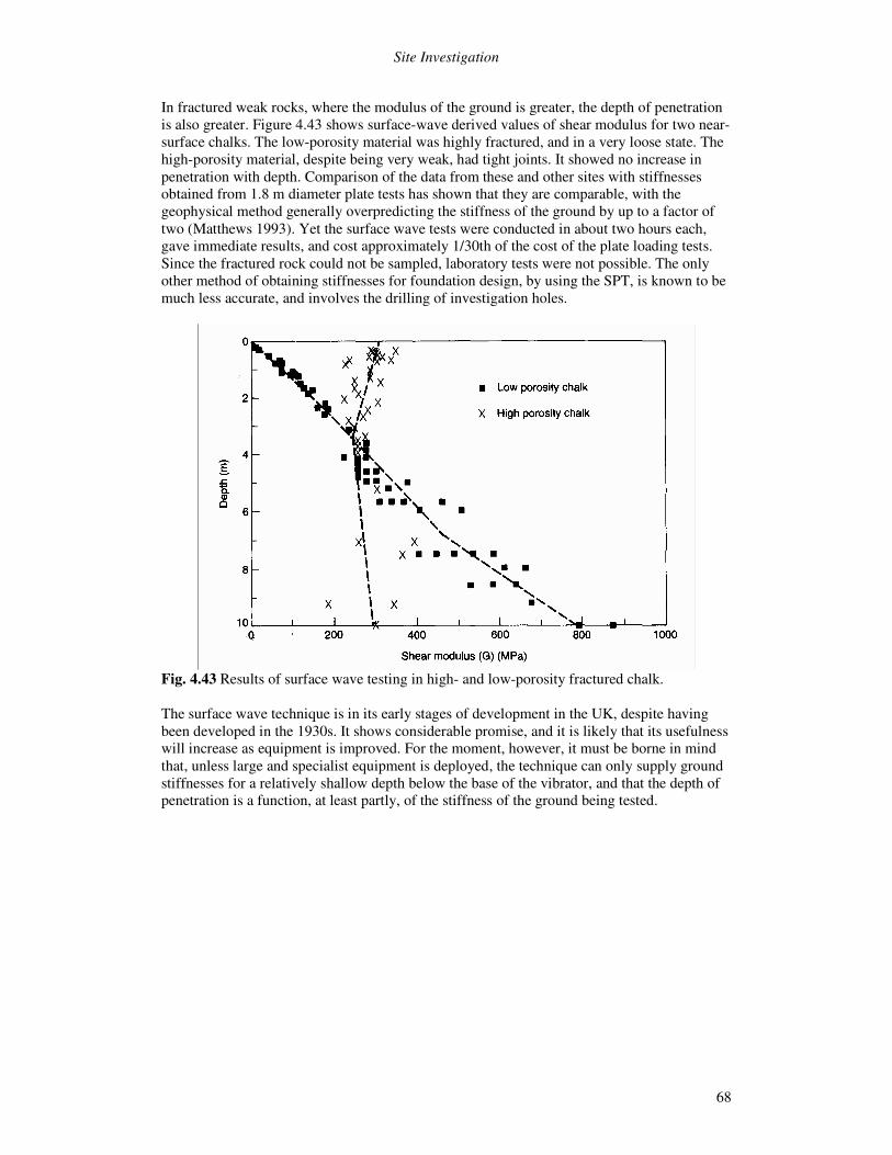
Site Investigation
68
In fractured weak rocks, where the modulus of the ground is greater, the depth of penetration is also greater. Figure 4.43 shows surface-wave derived values of shear modulus for two near-surface chalks. The low-porosity material was highly fractured, and in a very loose state. The high-porosity material, despite being very weak, had tight joints. It showed no increase in penetration with depth. Comparison of the data from these and other sites with stiffnesses obtained from 1.8 m diameter plate tests has shown that they are comparable, with the geophysical method generally overpredicting the stiffness of the ground by up to a factor of two (Matthews 1993). Yet the surface wave tests were conducted in about two hours each, gave immediate results, and cost approximately 1/30th of the cost of the plate loading tests. Since the fractured rock could not be sampled, laboratory tests were not possible. The only other method of obtaining stiffnesses for foundation design, by using the SPT, is known to be much less accurate, and involves the drilling of investigation holes.
Fig. 4.43 Results of surface wave testing in high- and low-porosity fractured chalk. The surface wave technique is in its early stages of development in the UK, despite having been developed in the 1930s. It shows considerable promise, and it is likely that its usefulness will increase as equipment is improved. For the moment, however, it must be borne in mind that, unless large and specialist equipment is deployed, the technique can only supply ground stiffnesses for a relatively shallow depth below the base of the vibrator, and that the depth of penetration is a function, at least partly, of the stiffness of the ground being tested.