Imaging passive seismic data

Brad Artmanbrad@sep.stanford.edu

Submitted toGeophysicsMarch 2005Stanford Exploration Project, Mitchell Building, Department of Geophysics,

Stanford University, Stanford, CA 94305-2215

ABSTRACT

Passive seismic imaging is the process of synthesizing the wealth of subsurface informa-tion available from reflection seismic experiments by recording ambient sound with anarray of geophones distributed at the surface. Cross-correlating the traces of such a pas-sive experiment can synthesize data that is immediately useful for analysis by the varioustechniques that have been developed for the manipulation ofreflection seismic data.With a correlation-based imaging condition, wave-equation shot-profile depth migrationcan use raw transmission wavefields as input to produce a subsurface image. For passivelyacquired data, migration is even more important than for active data because the sourcewavefields are likely weak and complex which leads to a low signal-to-noise ratio.Fourier analysis of correlating long field records shows that aliasing of the wavefields fromdistinct shots is unavoidable. While this reduces the orderof computations for correlationby the length of the original trace, the aliasing produces anoutput volume that may not besubstantially more useful than the raw data due to the introduction of cross talk betweenmultiple sources. Direct migration of raw field data can still produce an accurate imageeven when the transmission wavefields from individual sources are not separated.I illustrate the method with images from a shallow passive investigation targeting a buriedhollow pipe and the water table reflection. The images show a strong anomaly at the 1 mdepth of the pipe and faint events that could be the water table around 3 m. The imagesare not so clear as to be irrefutable. A number of deficienciesin the survey design andexecution are identified for future efforts.

INTRODUCTION

Passive seismic imaging is an example of wavefield interferometric imaging. In this case, thegoal is the production of subsurface structural images by recording the ambient noisefield ofthe Earth with surface arrays of seismometers or geophones.The images produced with thistechnique are directly analogous to those produced with thefamiliar conventional reflectionseismic experiment. Within the exploration seismic community, the words imaging and mi-gration are often used synonymously. Likewise, this paper presents the processing of passiveseismic data as a migration operation.

2

The idea of imaging the subsurface using subsurface sourceswas first introduced by Claer-bout (1968). That work provides a one-dimensional proof that the auto-correlation of timeseries collected on the surface of the Earth can produce the equivalent to a zero-offset timesection. Subsequently, Zhang (1989), used planewave decomposition to prove the result in 3Dover a homogeneous medium. Derode et al. (2003) develop the Green’s function of a heteroge-neous medium with acoustic waves via correlation and validates the theory with an ultrasonicexperiment. Wapenaar et al. (2004), through one-way reciprocity, prove that cross-correlatingtraces of the transmission response of an arbitrary medium synthesizes the complete reflectionresponse, i.e. shot-gathers, collected in a conventional active source experiment. Schuster etal. (2004) show that the Kirchhoff migration kernel to imagecorrelated gathers is identical tothat used to migrate prestack active data when one assumes that impulsive virtual sources arelocated at all receiver locations. In summary, it is now wellestablished that time differencescalculated by correlation are informative about the mediumbetween and below the receivers.

To distinguish data collected due to subsurface sources from conventional reflection seis-mic, the former are named transmission wavefields,T , and the latter reflection wavefields,R.The first section of this paper explains the basic kinematicsof extractingR from T . Next, I in-troduce the use of shot-profile wave-equation depth migration to create a subsurface structuralimage without first correlating the traces from the transmission wavefields.

One important attribute of truly passive data, is that the bulk of the raw data is likelyworthless. Useful seismic energy captured in the transmission wavefield could include randomdistributions of subsurface noise, down-hole sources, or earthquake arrivals. Assuming theyare not happening continuously, and not knowing when they occur, the passive seismologistmust continuously record. The ramifications of processing an entire passively recorded datavolume rather than individual wavefields from separate sources is explored through Fourieranalysis.

Finally, results from a small field experiment are presented. Passive data were recordedover several days on clean beach sand with a 2x2 meter array of72 geophones. A hollowpipe was buried beneath the array to provide an imaging target. Several data volumes fromdifferent times of the day and various pre-processing strategies were imaged to compare to anactive survey collected at the same location.

TRANSMISSION TO REFLECTION WAVEFIELDS

Figure 1, simplified for clarity, shows the basic kinematicsexploited in processing transmis-sion data. The figure includes two recording stations capturing an approximately planar wave-front emerging from a two-layer subsurface. Panel (a) shows the raypaths associated with thedirect arrival and one reflected both at the free surface and asubsurface interface. The secondtravel path (labeled reflection ray) has the familiar kinematics of the reflection seismic experi-ment if a source were excited at receiver one. The transmission wavefield is depicted in panel(b). Wavelet polarity is appropriate for direct arrivals and reflection. The three main featuresof transmission wavefields can be appreciated here. First, the exact timing of the arrival isunknown. Second, the phase and duration of transmitted energy are unknown and likely com-

3

plicated. Third, if the incident wavetrain coda is long, arrivals in the transmission record caninterfere.

Figure 1: (a) Approximately planararrival with rays showing importantpropagation paths for passive imag-ing. (b) Idealized traces from a trans-mission wavefield. (c) Shot-gather(reflection wavefield) synthesized us-ing trace r1 as the source. Manydetails are neglected for simplicity.Hopefully, these are explained satis-factorily in the text. sketch [NR]

r1 r1 r1 r2

(c)(b)sourc

e r

ay

reflection r

ay

time

lag

/twt

r1 r2r2r1

(a)

Choosing tracer1 as the comparison trace, panel (c) depicts the correlation spikes as-sociated with the arrivals in the data panel (b), where⊗ is correlation. A solid line withlinear move-out is super-imposed across the correlated traces corresponding to the direct ar-rival recorded at each receiver location. The dashed line onpanel (c) has hyperbolic moveout.However, no correlation peak exists on ther1⊗ r1 trace under the hyperbola. Not drawn, thesecond arrival onr2 will have a counterpart onr1 from a ray reaching the free surface farther tothe left of the model. In fact, the correlations produced from a single planewave will produceanother planewave.

However, each planar reflection is moved to the lag-time associated with a two-way tripfrom the surface to the reflector. Correlation removes the wait time for the initial arrivaland maintains the time differences between the direct arrival and reflections. Summing thecorrelations from a full suite of planewaves builds hyperbolic events through constructiveand destructive interference. Analyzing seismic data in terms of planewave constituents isa commonly invoked tool in seismic processing. Summing the correlations from incidentplanewaves is a planewave superposition process.

Passive seismic imaging is predicated on raypaths bouncingevery which-way from everydirection. Cartoons depicting the transmission experiment always leave something out thatcauses an inconsistency that needs more raypaths and receivers to explain. Unfortunately thetrend continues nearly forever. Such a complication ariseswith the inclusion of a second re-flector. The two reflection rays correlate with each other with a positive coefficient. The twotravel paths share the time through the shallow layer, so they correlate at a lag (or time dif-ference), equal to the two-way travel time through the deep layer. This correlation is not aproblem however. Part of the energy of the direct arrival will have made an intrabed multiplewithin the deep layer. This event has the opposite polarity compared to the direct arrival afteronce changing its propagation direction from↑ to ↓. The delay of its arrival at receiverr2compared to the direct arrival at receiverr1 is also the two-way travel time within the deeplayer. This correlation thus has the same lag as the one between the reflectors and oppo-site sign. Therefore, the internal multiple cancels potential artifacts of the correlation. This

4

shows the importance of modeling transmission data with a two-way extrapolator. Without allpossible multiples, correlation artifacts will quickly overwhelm the Earth structure within thecorrelated output.

Cross-correlation of each trace with every other trace handles the three main difficultiesof transmission data: timing, waveform, and interference.First, the output of the correlationis in lag units, that when multiplied by the time sampling interval, provide the time delaysbetween like events on different traces. The zero lag of the correlation is the zero time forthe synthesized shot-gathers. Second, each trace records the character and duration of theincident energy as it is reflected at the surface. This becomes the source wavelet analogous toa recorded vibrator sweep. Third, overlapping wavelets areseparated by correlation.

To calculate the Fourier transform of the reflection response of the subsurface,R(xr ,xs,ω),Wapenaar et al. (2004), proves

2ℜ[ R(xr ,xs,ω)] = δ(xs −xr )−∫

∂Dm

T (xr ,ξ ,ω)T ∗(xs ,ξ ,ω) d2ξ , (1)

where∗ represents conjugation. The vectorx will correspond herein to horizontal coordinates,where subscriptsr and s indicate different station locations from a transmission wavefield.After correlationr ands acquire the meaning of receiver and source locations, respectively,associated with an active survey. The RHS represents summing correlations of windows ofpassive data around the occurrence of individual sources from locationsξ . The symbol∂Dm

represents the domain boundary that surrounds the subsurface region of interest on which thesources are located. The transmission wavefieldsT (ξ ) contain the arrival and reverberationsdue to only one subsurface source. To synthesize the reflection experiment exactly, impulsivesources should completely surround the volume of the subsurface one is trying to image. Al-ternatively, many impulses can be substituted with a full suite of planewaves emerging fromall angles and azimuths as in the kinematic explanation above.

DIRECT MIGRATION

Artman and Shragge (2003) show the applicability of direct migration for transmission wave-fields. Artman et al. (2004) provide the mathematical justification for zero-phase source func-tions. Shragge et al. (2005) show results for the special case of imaging with teleseisms.Direct migration of transmission wavefields requires an imaging algorithm composed of wave-field extrapolation and a correlation based imaging condition. Shot-profile (Claerbout, 1971)wave-equation depth migration, described in Appendix A, fulfills these requirements.

Shot-profile migration uses one-way extrapolators to independently extrapolate up-going,U , and down-going,D, energy through the subsurface velocity model.U , extrapolated acausally,is a single shot-gather.D, extrapolated causally, is a wavefield modeled to mimic the sourceused in the experiment. I will define the causal extrapolation operator,E+, and the acausaloperator,E−. Wavefields are extrapolated to progressively deeper levels, z, by recursive ap-

5

plication of E±

Uz+1(kr ;xs,ω) = E−Uz(kr ;xs,ω) (2)

Dz+1(kr ;xs,ω) = E+Dz(kr ;xs,ω). (3)

wherekr is the wavenumber dual variable for receiver locationxr .

The imaging condition combines the two wavefields to output the subsurface image. Theimaging condition for shot-profile migration is defined as the zero lag of the cross-correlationof the two wavefields

iz(xr ) =∑

xs

∑

ω

Uz(xr ;xs,ω)D∗z (xr ;xs ,ω) . (4)

The sum over frequency extracts the zero lag of the correlation. The sum over shots,xs, stacksthe overlapping images from all the individual shot-gathers.

Extrapolation in the Fourier domain across a depth intervalis a diagonal matrix whose val-ues are phase shifts for each frequency-wavenumber component in the wavefield. Correlationof two equilength signals in the Fourier domain has one signal along the diagonal of a squarematrix multiplied by the second signal vector. As such, the two diagonal square operationsare commutable. This means that the correlation required tocalculate the Earth’s reflectionresponse from transmission wavefields can be performed after extrapolation as well as at theacquisition surface.

Table 1 pictorially demonstrates how direct migration of transmission wavefields fits intothe framework of shot-profile migration to produce the 0th and 1st depth levels of the zero-offset image. The correlation in the imaging condition takes the place of preprocessing thetransmission wavefield. The summations over shot locationsand frequency in equation 4 areomitted to reduce complexity. Note however, that the sum over shot locations is the same asthe integral over source locations in equation 1. Also, after the first extrapolation step, usingthe two different phase-shift operators, the two transmission wavefields are no longer identical,and can be redefinedU andD. This is noted with superscripts on theT wavefields at depth.The depth axis of the image is filled by recursive extrapolation of the wavefields followed byextracting the zero lag of the correlation.

Figure 2 compares the image produced by migrating raw transmission wavefields to onewhere synthesized shot-gathers by correlation were migrated. Transmission wavefields from225 impulsive sources across the bottom of the velocity model, Panel (c), were modeled witha two-way time-domain extrapolation program. The time sampling rate was 0.004 s, andthe source functions were Ricker wavelets with dominant frequency of 25 Hz. Panel (a) isthe image created by correlating each transmission wavefield (implementing equation 1) andmigrating the shot gathers by the algorithm described by theleft column of Table 1. Panel (b)was produced by migrating each transmission wavefield directly and summing the images asdescribed by the right column of Table 1. They are identical to machine precision.

T is the superposition ofU andD. Extrapolating the transmission wavefield with a causalphase-shift operator propagates energy recorded at the free surface which reflects downward

6

shot-profile migration transmission imagingUz=0(xr ;xs,ω) ⊗ Dz=0(xr ;xs,ω) = Tz=0(xr ;ξ ,ω) ⊗ Tz=0(xr ;ξ ,ω)

| | | |E− E+ E− E+

↓ ↓ ↓ ↓Uz=1(xr ;xs,ω) ⊗ Dz=1(xr ;xs,ω) = T −

z=1(xr ;ξ ,ω) ⊗ T +z=1(xr ;ξ ,ω)

Table 1: Equivalence of shot-profile migration of reflectiondata and direct migration of trans-mission wavefields.T (xr ,ξ , t) are the wavefields of equation 1.xs has a similar meaning toξ .∑

xs ,ξ and∑

ω produces the imageiz(xr ) for both methods. Only first and second levels of therecursive process are depicted.

Figure 2: (a) Correlation followed by migration. (b) Sum of all directly migrated transmissionwavefields. (c) Velocity model used for modeling and migration.dirmig [NR]

7

to become the source function for later reflections. This allows the use ofT in place ofD inshot-profile migration. Extrapolating the transmission wavefield with an acausal phase-shiftoperator reverse-propagates the upcoming events reflectedfrom subsurface structure. Thisallows the use ofT in place ofU in shot-profile migration.

In effect, the extrapolations re-datum the experiment to successively deeper levels in thesubsurface at which the wavefields are correlated in accordance with the general theory ofequation 1. The physics captured in the formulation of shot-profile migration remains the sameregardless of the temporal or areal characteristics of the initial conditions in the wavefields.

The extraction of only the zero lag of the correlation for theimage discards energy inthe two wavefields that is not collocated. This includes energy that has been extrapolatedin the wrong direction (since the same data is used initiallyfor both U and D wavefields).Conveniently, the only modification needed to make a conventional shot-profile migrationprogram into a transmission imaging program is to useT asD instead of a modeled wavefield.

Very important among the motivations for migrating transmission wavefields is the needto increase the signal-to-noise ratio of the output. If the experiment records only a smallamount of energy, the synthesized gathers from correlationcan be completely uninterpretable.The synthesized gather in the left panel of Figure 3 was produced the same 225 transmissionwavefields used in Figure 2, though each was convolved with a random source function. Thewavefields were individually correlated and summed. A few events centered around 4000 m,can be seen, but the gather is dominated by noise. In fact, this gather is full of useful energyhidden by the random source functions that the transmissionwavefields were convolved with.

The right panel of Figure 3 shows an image produced by direct migration of the transmis-sion wavefields followed by stacking the 225 images. An identical image, not shown, wasproduced by first correlating then migrating the synthesized gathers. Combining the weakredundant signal within each shot-gather with all of the others through migration produces avery good result despite the low quality of the shot-gather produced with the same data.

TRULY PASSIVE DATA

I differentiate passive seismic data from transmission wavefields when the timing of individ-ual sources are unknowable and possibly overlapping. For passively collected transmissionwavefields, the time axis and the shot axis are naturally combined. Field data can only beparameterizedTf (xr ,τ ) rather thanT (xr ,ξ , t) as dictated in equation 1. Withinτ , many in-dividual sources, and the reflections that occurt seconds afterward, are distributed randomlyacross the total recording time. Botht andτ represent the real time axis, though I will pa-rameterize wavefields with the understanding that max(t) is the two-way time to the deepestreflector of interest andτ is the time axis from the beginning to the end of the total recordingtime. The difficulty in separating the data into constituentwavefields from a single source,paramaterizing as function ofξ , comes from not knowing the time separation between eventsand the possibility that they may overlap.

If it is impossible to separate field data into individual wavefields, transforming the long

8

Figure 3: Left: Correlated gather synthesized from a passive data set over the syncline modelwith random source functions of various lengths. Right: Zero-offset migration of the datafrom the left panel produced by direct migration.migcor [NR]

data to the frequency domain has important ramifications on further processing. The definitionof the discrete Fourier transform (DFT) for an arbitrary signal f (τ ) can be evaluated for aparticular frequency ,

F| = DFT[ f (τ )]| =1

√nτ

nτ∑

τ

f (τ )e−iτ . (5)

wherenτ is the number of samples inf . The frequency domain dual variable ofτ is , andI will use ω for the frequency domain dual variable oft . If the long function f (τ ) is brokeninto N sections,gn(t), of length max(t), the amplitude of the same frequencycan also becalculated

F| =1

√N

N∑

n=1

DFT[gn(t)]|ω =1

√N

DFT[N

∑

n=1

gn(t)]|ω (6)

by simply changing the order of summation for convenience and scaling the result.

The only requirement for the equation above is that the two different length transformscontain the particular frequency being calculated (i.e. a frequency where = ω is possibleas dictated by the Fourier sampling theorem). The center equality of equation 6 (the sum ofshort transforms), shows that frequencies common to the twotransforms are identical aftera simple amplitude scaling. The right equality (the sum of time windows) shows that thelong transform stacks the constituent windows at common frequencies. The two alternativesinterpreted together show that subsampling the long transform aliases the time domain. Thisrelationship between sampling and aliasing between a signal’s representation in two domains

9

is the Fourier dual to subsampling a time signal in order to reduce its Nyquist frequency at therisk of aliasing high frequencies.

Passive seismic field data,Tf (τ ), takes the role of the general signalf (τ ), and thegn(t)are T (xr ,ξ , t)|ξ=n (as well as background noise between sources). The center equality ofequation 6 states thatTf (xr ,ω) is a subset fromTf (xr , ). The right equality states that

Tf (xr , t) =∑

ξ

T (xr ,ξ , t) . (7)

With the relationships in equation 6, implementing a singlecorrelation of passive field datadoes not produceR, but some unknown quantityR

R(xr ,xs , ) =1

NTf (xr ,ω)T ∗

f (xs ,ω) (8)

whereN is the number of lengtht time windows into which the total recording time can bedivided, andTf can be calculated with equation 7. The relationship is undefined at frequencies 6= ω.

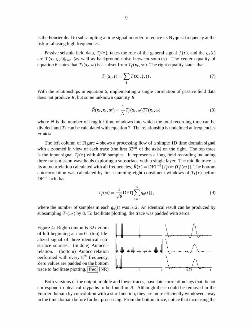
The left column of Figure 4 shows a processing flow of a simple 1D time domain signalwith a zoomed in view of each trace (the first 32nd of the axis) on the right. The top traceis the input signalTf (τ ) with 4096 samples. It represents a long field recording includingthree transmission wavefields exploring a subsurface with asingle layer. The middle trace isits autocorrelation calculated with all frequencies,R(τ ) = DFT−1[Tf ( )T ∗

f ( )]. The bottomautocorrelation was calculated by first summing eight constituent windows ofTf (τ ) beforeDFT such that

Tf (ω) =1

√8

DFT[8

∑

n=1

gn(t)] , (9)

where the number of samples in eachgn(t) was 512. An identical result can be produced bysubsamplingTf ( ) by 8. To facilitate plotting, the trace was padded with zeros.

Figure 4: Right column is 32x zoomof left beginning att = 0. (top) Ide-alized signal of three identical sub-surface sources. (middle) Autocor-relation. (bottom) Autocorrelationperformed with every 8th frequency.Zero values are padded on the bottomtrace to facilitate plotting.freq [NR]

Both versions of the output, middle and lower traces, have late correlation lags that do notcorrespond to physical raypaths to be found inR. Although these could be removed in theFourier domain by convolution with a sinc function, they aremore efficiently windowed awayin the time domain before further processing. From the bottom trace, notice that increasing the

10

decimation factor to 16 would alias the symmetric, acausal lags into the reflection response.To avoid this problem, the short time windows need to be more than twice as long as the timeto the deepest reflection of interest. In this example the first two correlations ofR equalR.Producing the bottom trace involvesO(10) less computations than the middle trace.

Wavefield summation

Unfortunately, the beginning ofR is not alwaysR. The stacking of wavefields implicit inprocessing field data can be explored by considering field data composed of transmissionwavefieldsa(xr , t) andb(xr , t) from individual sources. Like the input trace of Figure 4, theyare placed on the field record at unknown timesτa andτb such that

Tf (τ ) = a ∗ δ(t − τa)+b ∗ δ(t − τb). (10)

Correlation in the Fourier domain to implement equation 8 yields

Tf T ∗f = AA∗ + B B∗ + AB∗e−iω(τa−τb) + B A∗e−iω(τb−τa ) . (11)

The sum of the first two terms is the result dictated by equation 1. The last two terms arecross talk. If|τb − τa| > max(t), one term is acausal, and the other is at late lags that canbe windowed away in the time domain. This was the case in the middle trace of Figure 4.If |τb − τa| < max(t), the cross terms are included in the correlated gathers. Inlight of theprevious section, the last scenario will be the predominantsituation if the source delaysτa andτb are truly random. Figure 4, however, is not a fair representation of field data because valuesfor τa,b were very carefully selected.

RedefineA and B as the impulse response of the Earth,Ie, convolved with source func-tions,F , which now contain their phase delays. As such, the cross terms of equation 11 are

AB∗ = (Fa Ie)(Fb Ie)∗ = Fa F∗b I 2

e = Fc I 2e . (12)

Like the first two terms in equation 11, the cross terms contain the desired information aboutthe Earth. However, the source functionfc included is not zero phase. These terms may be theother-terms or virtual multiples mentioned in Schuster et al. (2004). Ifthe source functionsare random series, terms with residual phase (Fc I 2

e ) within the gathers will decorrelate anddiminish in strength as the length off and the number of cross terms increases. While wemay hope to collect a large number of sources, it is probably unreasonable to expect many ofthem to be random series of great length. This is not probableif the noise sources have similarsource mechanisms.

The inclusion of these cross terms in the correlation explains why R produced with equa-tion 8 is not equivalent toR from equation 1. Virtual multiple events due tons sources willlikely be more problematic than conventional multiples as every reflector can be repeatedns !/(ns −2)! times. The ratio of desirable zero phase terms,Ie, to cross terms,Fj I 2

e , decreasesas 1/(ns −1) if the source terms contain the same wavelet.

Figure 5 shows the effect of the cross terms when calculatingcorrelations. The figureis directly analogous to Figure 4, though with a more realistic input trace. First, there are

11

overlapping source-reflection pairs: the second source arrives at the receiver before the re-flection from the first source. Second, the direct arrivals are spaced randomly along the timeaxis in contrast to Figure 4 where the direct arrivals were placed at samples 1, 513, and 2049.That contrivance allowed the summing of constituent time windows 256 or 512 samples longwithout introducing residual phase functions as describedin equation 12.

Figure 5: Right column is 32x zoomof left beginning att = 0. (top) Ide-alized signal of three identical sub-surface sources. First two source-reflection pairs overlap. (middle) Au-tocorrelation. (bottom) Autocorrela-tion performed after stacking 8 con-stituent windows. Zero values arepadded on the bottom trace to facil-itate plotting. freq2 [NR]

The result desired by a passive seismologist trying to produce a zero-offset trace fromR,bottom trace Figure 4, can not be produced from the top trace in Figure 5. The middle tracewas correlated with inputT ( ). The bottom autocorrelation was computed after first stackingeight constituent windows. In contrast to the two autocorrelations in Figure 4, not even theearly lags are the same. The presence of more aphysical correlations in the middle trace forthis example has caused the symmetric peaks at late lags to bealiased into the early lags of thebottom result at this level of decimation. Both methods produce the wrong result at almost alltimes. They are however correct and identical at zero lag.

This analysis shows that without invoking long, purely random source functions, a singlecorrelation of passive data will not model shot-gathers from a reflection survey. In the nextsection, 2D synthetic data are used to show the extent of the problem and the ability of directmigration to produce a correct subsurface image despite thesummation of wavefields.

Examples with synthetic data

To demonstrate the effects of wavefield summation, two synthetic acoustic passive data sets areused. Transmission wavefields from 225 impulsive sources across the bottom of the velocitymodels were propagated with a two-way extrapolation program as before. To then simulatea passive recording campaign, a unique source function was convolved with each wavefieldbefore summing all of them together. The total length of the source function trace mimics theduration of the recording campaign. The shape, time location, and length of the wavelet usedwithin the source function trace, otherwise zero, embodiesmy assumptions on the nature ofthe ambient subsurface noisefield. The source functions incorporate many of the features ofthe toy example in Figures 4 & 5.

Figure 6 shows synthetic data from a model containing two diffractors in a constant ve-locity medium. Panel (a) is a transmission wavefield from a subsurface source below the far

12

left of the model, while the source in panel (b) was belowx = 5000 m. Source wavelets were50 ms long, with dominant frequency of 25 Hz, and placed on thetime axis to align theirdirect arrivals. This experiment is the 2D analog to Figure 4. The total length of the sourcefunctions were the same as the modeled time axis. Panel (c) is the sum of all 225 similarwavefields from shots below the entire width of the acquisition. The coherent summation ofthe direct arrivals makes a strong planewave att ∼ 0.6 s, and the diffractors are well cap-tured through constructive interference. Cross talk between the wavefields has been canceledthrough destructive interference. The summed wavefield below the strong planewave is thesame as would be collected from a zero-offset reflection experiment. Correlation of the tracesin panel (c) does not produce shot-gathers. Instead, eachxs plane fromR contains a series ofplanewaves that completely mask the diffractors. The slicefrom the correlated volumexs = xr

is however interpretable. The autocorrelation produces a result similar to panel (c) where theplanewave is moved fromt ∼ 0.6 s to zero lag.

Figure 6: (a) Transmission wavefield from a source below 1200 m in a model containing twodiffractors. (b) Transmission wavefield from source below 5000 m. (c) Sum of 225 modeledwavefields.diff.noshift [NR]

In contrast, Figure 7 shows synthetic data from the the same model with the additionof random phase delays for the source functions throughout the experiment. Panels (a)-(c)correspond to the same panels in the previous figure. The strong planewave and coherentdiffractors from Figure 6 have been replaced by an uninterpretable superposition. Correlatingtraces from this wavefield returnsR that is completely unusable rather than the reflectionwavefieldR. This is the 2D equivalent to Figure 5.

Data was also synthesized through a model containing two synclines. Source functionswere identical to those used for the diffractor exercise above. Figure 8 shows summed wave-fields with, panel (a), and without, panel (b), correcting for the onset time of the 225 subsur-face sources. Again, correlating the superposition of wavefields, from either panel, returns anunusable data volume rather than shot-gathers fromR.

13

Figure 7: (a) Transmission wavefield from a source below 1200 m in a model containing twodiffractors. (b) Transmission wavefield from source below 5000 m. (c) Sum of all wavefields.diff.shift [NR]

Figure 8: (a) Perfectly stacked shots from a double syncline model. (b) Stack of wavefieldswith random onset times.dat.syn [NR]

14

plane-wave migration wavefront imaging(∑

xsUz=0(xr ;xs,ω)

)

⊗(∑

xsDz=0(xr ;xs,ω)

)

= Tz=0(xr ,ω) ⊗ Tz=0(xr ,ω)| | | |

E− E+ E− E+

↓ ↓ ↓ ↓Uz=1(xr ,ω) ⊗ Dz=1(xr ,ω) = T −

z=1(xr ,ω) ⊗ T +z=1(xr ,ω)

Table 2: Equivalence between direct migration of passive field data and simultaneous migra-tion of all shots in a reflection survey. Only first and second levels of the iterative process aredepicted.

∑

ω produces the imageiz for both methods.

DIRECT MIGRATION OF PASSIVE DATA

Using equation 8 to correlate field data (not being able to collect T as a function of individualsource functions), we cannot process the result of the correlation with conventional reflectiondata tools. Without knowing the exact timing of all the source functions, it is not possible tocompletely eliminate all time delays as shown in equation 11. However, the field data can stillbe migrated with a scheme that includes extrapolation and a correlation imaging condition.

Shot-profile depth migration produces the correct image if the source wavefield,D, iscorrect for the data wavefield,U . Shot-profile migration becomes planewave migration ifall shot-gathers are summed for wavefieldU , and a horizontal planar source is modeled forwavefieldD. The wavefield in Figure 6c could be successfully imaged witha planewave att = 0.6s modeled for the wavefieldD.

This method can introduce cross talk between the individualexperiments while attemptingto process them all together. Complete areal distribution of sources will cancel the cross talkthrough destructive interference and synthesize a zero-offset data acquisition. The informationlost in this sum is the redundancy across the offset axis. Forsimple structural imaging, thezero-offset image is satisfactory, though for more complicated mediums and further processinga full plane-wave migration can be implemented (Sun et al., 2001; Liu et al., 2002).

Table 2 pictorially demonstrates how direct migration of field passive data fits into theframework of plane-wave migration analogous to Table 1. Moving the sum over shots inthe imaging condition, equation 4, to operate on the wavefields rather than their correlation,changes shot-profile migration to planewave migration where a horizontal planar source ismodeled for wavefieldD. As shown above, the Fourier transform of passive field data sim-ilarly sums the shot axis. The source function built by this action will have some temporaltopography in this case as compared to planewave migration for the controlled experiments.

Figure 9 shows zero-offset images produced by direct migration of the data shown in Fig-ure 8 respectively. The quality of panel (a) is equivalent to a zero-offset reflection migration.Dipping reflectors and sharp changes in slope produce migration tails. Panel (b) is a remark-ably clean image given the appearance of the input data, though not as high quality as itscounterpart. A faint virtual multiple mimicking the first event can be seen atz = 350 m. The

15

physical multiple from the first reflector atz = 485 m is very dim (which actually highlightsthe second reflector that gets masked in the previous panel).

Figure 9: (a) Zero-offset image produced by direct migration of data in Figure 8a. (b) Zero-offset image produced by direct migration of data in Figure 8b. mig.syn.norand2[NR]

The length of the source functions used to synthesize the data were equal to the modelingtime of the transmission wavefield. Thus, summing the wavefields as dictated by equation 7does not allow for the requirement that the wavefields shouldbe at least twice as long as max(t)to avoid aliasing the symmetric acausal lags. The short timeaxis also allows late time eventsto wrap around the time axis when applying the random phase delays. For these reasons, theimage in Figure 9b represents a worst-case scenario of careless data preparation.

FIELD EXPERIMENT

Cross-correlating seismic traces of passively collected wavefields has a rich history pertainingto the study of the sun (Duvall et al., 1993). On Earth thus far, only two dedicated field cam-paigns to test the practicality of passive seismic imaging can be found in the literature: Baskirand Weller (1975), and Cole (1995). Neither experiment produced convincing results. Withthe hope that hardware limitations or locality could explain their lack of success, I conducteda shallow, meter(s) scale, passive seismic experiment in the summer of 2002. Seventy-two40 Hz geophones were deployed on a 25 cm grid on the beach of Monterey Bay, Californialinked to a Geometrics seismograph. The experiment was combined with an active investiga-tion of the same site using the same recording equipment and asmall hammer (Bachrach andMukerji, 2002). A short length of 15 cm diameter plastic pipewas buried a bit less than onemeter below the surface. The array was approximately 100 meters from the water’s edge. Thewater table is approximately three meters deep. The velocity of the sand, derived from theactive survey, was a simple gradient of 180 to 290 m/s from thesurface to the water table, andthen 1500 m/s.

16

Figure 10 shows the time-migrated active source image with aclear anomaly associatedwith the hollow pipe and the water table. A simple RMS gradient velocity to the water tablewas used for imaging. The high quality of the beach sand allowed usable signal to as high as1200 Hz for that survey.

Figure 10: In-line, x, and crossline, y, time migrated active seismic image. The hollow pipecauses an over-migrated anomaly at 12ms, 19m in the inline (X) direction. A strong watertable reflection is imaged at 28ms. After Bachrach, 2003.active [NR]

Passive data was collected over the course of two days two weeks later. Due to the lim-itations of the recording equipment, only one hour of data exist from the campaign. Theseismograph was only able to buffer several seconds of data in memory before writing to afile. The time required to write, reset and re-trigger happened to be about 5 times greater thanthe length of data captured depending on sample rates. Data was collected at several samplingrates. Through the course of the experiment, we found it possible to fly a small kite (plasticgrocery bag) that would continuously move the triggering wire over the hammer plate to trig-ger the system automatically as soon as it was ready to record. The individual records werethen spliced together along the time axis to produce long traces. The gaps in the traces do notinvalidate the assumptions of the experiment as long as the individual recordings are at leastas long as the longest two-way travel time to the deepest reflector.

Because the array was only eight by nine stations, shot-gathers produced by correlation,even when resampled as a function of radial distance from thecenter trace, had too few tracesto find consistent events. Migrating the data, as described above, provides both signal to noiseenhancement, as well as interpolation. In this case, five empty traces were inserted betweenthe geophone locations for processing, as shown in Figure 11. As the data are extrapolatedthrough the velocity model, the energy on the live traces moves laterally across to fill theempty traces. After the distance propagated is approximately equal to the separation betweenlive traces, wavefronts have coalesced into close approximations to their expression if the data

17

were first interpolated.

Figure 11: A small time window of in-line and crossline sections of a raw passive transmissionwavefield inserted on a five times finer grid for migration.raw [NR]

Data were collected to correspond to distinct environmental conditions through the courseof the experiment. Afternoon data was collected during highlevels of cultural activity andwind action. Night data had neither of these features, whilemorning data had no appreciablewind noise. In all cases the pounding of the surf remained mostly consistent. By processingdata within various time windows, it was hoped that images ofthe water table at differentdepths could be produced. However, given the 2 m maximum offset of the array, ray parame-ters less than 17o from the vertical would be required to image a 3 m table reflector at the verycenter of the array. Very little energy was captured at such steep incidence angles. Had we notbeen so careful not to walk around the array during recording, this might not have been thecase.

Figures 12-14 show the images produced during the differenttimes of the day. Approxi-mately five minutes of 0.001 seconds/sample data were used toproduce each image by directmigration. Usable energy out to 450 Hz is contained in all thedata collected. Abiding bythe 1/4 wavelength rule, and using 200 m/s with 400 Hz, the data should resolve targets to∼ 0.125 m. Other data volumes corresponding to various fasterand slower sampling rateswere processed, though these results are the most pleasing.

Pre-processing in most cases consisted of a simple bandpassto eliminate electrical gridharmonics, as the higher octaves carry the only useful signal considering the low velocityof the beach sand and the small areal extent of the array. Figure 12 is the image producedmid-day. The two panels are thex and y sections corresponding to the center of the buriedpipe. Figure 13 was produced with data from around midnight.The image planes are thesame as for the previous figure. One dimensional spectral whitening was also tried, though thesimple application remained stable only during the night acquisition. Figure 14 was produced

18

with the whitened version of the data used for the previous figure. Notice the instability atshallow depths before the wavefront healing has interpolated across the empty traces. Datacollected in the morning did not yield appreciably different images from the night data towarrant inclusion.

Figure 12: Migrated image from passive data collected during the windy afternoon. In-lineand crossline depth section extracted at the coordinates ofthe buried pipe.daybp [NR]

All output images contain an appreciable anomaly at the location of the buried pipe. Com-plicating the interpretation of the results, the ends of thepipe were not sealed before burial.After two weeks under the beach, it is impossible to know how much of the pipe was filled,which would destroy the slow, air-filled target. Future experiments would also incorporatetarget with a severe angle that could clearly stand out.

In the whitened night data image and the bandpassed day data image, there is hint of areflector at depth that could be the water table. High tide on that day was at 4:30 in theafternoon, and fell to low tide at about 8:30pm, and thus the relative change of this hint of areflector is consistent. However, due to the limitations of the array discussed above, and thelack of strength and continuity along the crossline direction, I do not hold this to be a veryreliable interpretation.

Discussion

Draganov et al. (2004) systematically explores the qualityof a passive seismic processing ef-fort as a function of the number of subsurface sources, the length of assumed source functions,and migration. Rickett and Claerbout (1996) identify increasing the signal-to-noise ratio bythe familiar 1/

√n factor wheren can be time samples in the source function, or number of

subsurface sources captured in the records. Migration sumsthe information each shot-gathercontains about a specific subsurface location to the same point in the image. Therefore, while

19

Figure 13: Migrated image from passive data collected during the night. In-line and crosslinedepth section extracted at the coordinates of the buried pipe. nightbp [NR]

Figure 14: Migrated image from passive data collected during the night. One dimensionalspectral whitening applied before migration to the same rawdata used in Figure 13. In-lineand crossline depth section extracted at the coordinates ofthe buried pipe.nightd [NR]

20

a correlated gather may not look like it contains useful information, migrating that data canproduce interpretable results.

The direct controls available to increase quality of passive seismic effort are the length oftime data is collected, and the number of receivers fielded for the experiment. If the naturalrate of seismicity within a field area is constant, accumulation of sufficient signal dictates howlong to record. Not surprisingly, increasing the total length of time of the source traces for thesynthetic data described above does not change the quality of the output. If all the sources areused with the same source functions, this only adds quiet waiting time between the events thatcontributes neither positively nor negatively to the output. This experiment implies a changingrate of seismicity. When interpreting the increase in signal by factor 1/

√t with application to

short subsurface sources,t represents the mean length of the source functions rather than totalrecording time. Assuming some rate of subsurface sources associated with each field site, thetotal recording time will control the quality of the output by 1/

√ns wherens is the number of

sources captured.

Another method to increase the quality of the experiment is to migrate more traces. Mi-gration facilitates the constructive summation of information captured by each receiver in thesurvey. Therefore, more receivers sampling the ambient noisefield results in more constructivesummation to each image location in the migrated image. In this manner migration increasesthe signal-to-noise ratio of a subsurface reflection by the ratio 1/

√r , wherer is the number of

receivers that contain the reflection. This allows the production of very interpretable imagesdespite the raw data or correlated gathers showing little promise.

Definitive parameters for the numbers of geophones required, and sufficient length of timeto assure quality results for a passive seismic experiment are ongoing research topics as fewfield experiments have yet been analyzed. It is clear however, that an over-complete samplingof the surficial wavefield is required, and that the length of time required will be dictated on theactivity of the local ambient noisefield. Considering the layout of equipment, over-completesampling means that more receivers are better, and areal arrays are much better than linearones. This can be understood by considering a planewave propagating along an azimuth otherthan that of a linear array. After the direct arrival is captured, the subsequent reflection pathpierces the Earth’s surface again in the crossline direction away from the array. With a 2.5Dapproximation, the apparent ray parameter of the arrival will suffice given an areally consistentand planar source wave. Because the true direct arrival associated with a reflection travel-pathwas not recorded, the possibility of erroneous phase delaysand wavelets could distort theresult.

CONCLUSION

If time-localized events are present, such as teleseismic arrivals, one can process small timewindows when sure of significant contribution to the image. Without knowledge of if or howmany sources are active within the bulk of passive data, longcorrelations of the raw data arean inevitable approximation, equation 8, to the rigorous derivation, equation 1. Fortunately,first aliasing the short time records reduces the computation cost for a DFT by 1/nτ wherenτ

21

is the number of samples in the long input trace. The trace length will be O(107) for just oneday of data collected at 0.004 s sampling rate.

The aliasing implicit in not separating individual wavefields for processing sums the sourcefunctions within the output. This superposition does not produceR(xr ,xs,ω) by correlation ifsource functions are not random. Instead, passive data can only be processed by direct migra-tion with an algorithm that can accept generalized source functions (parameterized by spaceand time), and uses a correlation imaging condition. Both ofthese conditions are enjoyed byshot-profile migration. Direct migration also saves substantial computation cost sinceO(n2)traces are produced by cross-correlatingn receivers from a passive array.

Migrating all sources at the same time removes the redundantinformation from a reflectoras a function of incidence angle. This makes velocity updating after migration impossible.At this early stage, I contend that passive surveys will onlybe conducted in actively studiedregions where very good velocity models are already available. If this becomes a severe limit,the incorporation of plane-wave migration strategies can fill the offset dimension of the image.

Finally, moving the extraction of the reflection response from the transmission wavefielddown to the image point during migration also introduces thepossibility for more advancedimaging conditions, such as deconvolution, and other migration strategies, such as convertedmode imaging.

Acknowledgments

Thanks to my colleagues and advisors at Stanford Universityfor insightful discussions anddevelopment of the infrastructure to perform these experiments. I thank Deyan Draganov ofDelft University for successful collaboration and his modeling efforts. Ran Bachrach pro-vided the Michigan State shallow seismic acquisition equipment for the beach experiment aswell as his image from his active seismic experiment. Emily Chetwin and Daniel Rosaleshelped collect data on the beach. Partial funding for this research was enjoyed from PetroleumResearch Fund grant ACS PRF#37141-AC 2, the Stanford Exploration Project and NationalScience Foundation grant number 0106693 to S.L. Klemperer and J. Claerbout. Many thanksto my patient reviewers whose constructive comments greatly improved the quality of thismanuscript.

REFERENCES

Artman, B., and Shragge, J., 2003, Passive seismic imaging:AGU Fall Meeting, Eos Trans-actions of the American Geophysical Union, Abstract S11E–0334.

Artman, B., Draganov, D., Wapenaar, C., and Biondi, B., 2004, Direct migration of passiveseismic data: 66th Conferance and Exhibition, EAGE, Extended abstracts, P075.

Bachrach, R., and Mukerji, T., 2002, The physics of seismic reflections within unconsolidatedsediments: Technology for near surface 3D imaging using dense receiver array: AGU FallMeeting, Eos Transactions of the American Geophysical Union, Abstract T22B–1141.

22

Baskir, C., and Weller, C., 1975, Sourceless reflection seismic exploration: Geophysics,40,158.

Claerbout, J. F., 1968, Synthesis of a layered medium from its acoustic transmission response:Geophysics,33, no. 2, 264–269.

Claerbout, J. F., 1971, Toward a unified theory of reflector mapping: Geophysics,36, no. 03,467–481.

Claerbout, J. F., 1985, Migration:,in Imaging the Earth’s Interior Blackwell Scientific Publi-cations, 1–74.

Cole, S. P., 1995, Passive seismic and drill-bit experiments using 2-D arrays: Ph.D. thesis,Stanford University.

Derode, A., Larose, E., Campillo, M., and Fink, M., 2003, Howto estimate the Green’s func-tion of a heterogeneous medium between two passive sensors?Application to acousticwaves: Applied Physics Letters,83, no. 15, 3054–3056.

Draganov, D., Wapenaar, K., and Thorbecke, J., 2004, Passive seismic imaging in the presenceof white noise sources: The Leading Edge,23, no. 9, 889–892.

Duvall, T., Jefferies, S., Harvey, J., and Pomerantz, M., 1993, Time-distance helioseismology:Nature,362, 430–432.

Gazdag, J., and Sguazzero, P., 1984, Migration of seismic data by phase-shift plus interpola-tion: Geophysics,49, no. 02, 124–131.

Liu, F., Stolt, R., Hanson, D., and Day, R., 2002, Plane wave source composition: An accuratephase encoding scheme for prestack migration: SEG, 72nd Annual International Meeting,1156–1159.

Rickett, J., and Claerbout, J., 1996, Passive seismic imaging applied to synthetic data: StanfordExploration Project - Annual Report,92, 83–90.

Rickett, J. E., and Sava, P. C., 2002, Offset and angle-domain common image-point gathersfor shot-profile migration: Geophysics,67, no. 03, 883–889.

Schuster, G., Yu, J., Sheng, J., and Rickett, J., 2004, Interferometric/daylight seismic imaging:Geophysics Journal International,157, 838–852.

Shragge, J. C., Artman, B., and Wilson, C., 2005, Teleseismic shot-profile migration: Geo-physics,accepted for this issue.

Sun, P., Zhang, S., and Zhao, J., 2001, An improved plane waveprestack depth migrationmethod: SEG, 71st Annual International Meeting, 1005–1008.

Wapenaar, K., Thorbecke, J., and Draganov, D., 2004, Relations between reflection and trans-mission responses of three-dimensional inhomogeneous media: Geophysical Journal Inter-national,156, 179–194.

23

Zhang, L., 1989, Reflectivity estimation from passive seismic data: Stanford ExplorationProject- Annual Report,60, 85–96.

24

APPENDIX A

MIGRATION

Migration produces a subsurface image from many seismic experiments collected on a conve-nient datum (usually the surface of the Earth). Each shot collected in a survey carries redun-dant information about subsurface reflectors. Collapsing this redundancy to specific locationsin the subsurface by migration makes a structural image beneath the survey. For this reason,the words imaging and migration are used interchangeably. Of the many migration strategiesavailable, this discussion centers on shot-profile depth migration. Depth migration is a cascadeof extrapolation and imaging.

Extrapolation

The wave equation describes the propagation of seismic energy through a medium. The scalarsimplification of the equation describes the propagation ofcompressional waves through anacoustic medium. While this simplification is not necessary, it is an established, robust, andconvenient framework for this discussion. A wavefield is extrapolated from an initial conditionto a close approximation of its state at a different locationor time using a one-way propagatorderived in Claerbout (1985).

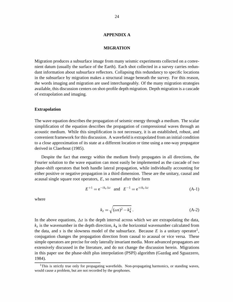
Despite the fact that energy within the medium freely propagates in all directions, theFourier solution to the wave equation can most easily be implemented as the cascade of twophase-shift operators that both handle lateral propagation, while individually accounting foreither positive or negative propagation in a third dimension. These are the unitary, causal andacausal single square root operators,E , so named after their form

E+1 = e−ikz1z and E−1 = e+ikz1z (A-1)

where

kz =√

(ωs)2 − k2x . (A-2)

In the above equations,1z is the depth interval across which we are extrapolating the data,kz is the wavenumber in the depth direction,kx is the horizontal wavenumber calculated fromthe data, ands is the slowness model of the subsurface. BecauseE is a unitary operator1,conjugation changes the propagation direction from causalto acausal or vice versa. Thesesimple operators are precise for only laterally invariant media. More advanced propagators areextensively discussed in the literature, and do not change the discussion herein. Migrationsin this paper use the phase-shift plus interpolation (PSPI)algorithm (Gazdag and Sguazzero,1984).

1This is strictly true only for propagating wavefields. Non-propagating harmonics, or standing waves,would cause a problem, but are not recorded by the geophones.

25

The goal of migration is to approximately reverse the seismic experiment with a doubleextrapolation process. The up-coming energy of a single shot-gather,Uz=0, is the jth shot-gather from the total reflection experiment located atxsj transformed to wavenumber,kr :

Uz=0(kr ;xsj ,ω) = R(kr ,xs = xsj ,ω). (A-3)

Each gather is iteratively extrapolated byE−1 to all desired depth levelsz > 0

Uz+1(kr ;xsj ,ω) = E−Uz(kr ;xsj ,ω). (A-4)

The phase-shift ofE−1 subtracts time from the beginning of the experiment and collapsescurvilinear wavefronts in order to model the wavefield as if it were collected at a deeper level.

The down-going energy for a particular shot is a modeled wavefield, Dz=0(xr ;xsj ,ω), ofzeros with a single trace source wavelet (at time zero) at thesource locationxsj . This wavefieldis transformed to wavenumber and extrapolated with the causal phase-shift operatorE+ to alldesired levelsz > 0

Dz+1(kr ;xsj ,ω) = E+Dz(kr ;xsj ,ω). (A-5)

The phase-shift adds time to the onset of experiment corresponding to the travel time requiredfor the energy of the source to reach progressively deeper levels of the Earth across allxr

locations. If an areal source, such as a length of primachordor 30 Vibroseis trucks, were usedinstead of a point source,Dz=0 should be modeled to reflect the appropriate source function.

This double extrapolation process is performed for each individual shot experiment to alldepth levels of interest. Instead of reducing the complexity and volume of the original data, theprocess greatly increases the volume by maintaining the separation of up-coming and down-going energy through all depth levels for all time for all thereceivers recording each shot.

Imaging

The imaging aspect of migration compares the energy in theD andU wavefields at each sub-surface location to output a single subsurface model (Claerbout, 1971). The operator used toaccomplish this goal is called the imaging condition. Whiledifferent migration schemes re-quire subtly different imaging conditions, the following discussion focuses on the one requiredfor shot-profile depth migration.

Reflectors are correctly located in the image,iz(x,h), at every depth levelz as a functionof horizontal position,x, and offset,h, when energy in the two wavefields is collocated. Thiscondition maps energy to the image when the source has reached the location where a reflec-tion was produced. Last, the entire model space is populatedby summing the results of all theimages produced in this manner by each shot collected in the survey (Rickett and Sava, 2002)

iz(x,h) = δx,xr

∑

xsk

∑

ω

Uz(xr +h;xsk ,ω)D∗z (xr −h;xsk ,ω) . (A-6)

26

The Kronecker delta function indicates that the surface coordinates of the wavefields,xr , arealso used for the image. Notice that the zero lag of the correlation is calculated by summingover frequency. Evaluating the imaging condition at each depth to which the data and sourcewavefields have been extrapolated produces a structural image of the subsurface correspondingto changes in material properties.