essays on dynamic pricing

Washington University in St. LouisWashington University Open Scholarship

Arts & Sciences Electronic Theses and Dissertations Arts & Sciences

Summer 8-15-2013

Essays on Dynamic PricingKoray CosgunerWashington University in St. Louis

Follow this and additional works at: https://openscholarship.wustl.edu/art_sci_etds

Part of the Business Commons

This Dissertation is brought to you for free and open access by the Arts & Sciences at Washington University Open Scholarship. It has been acceptedfor inclusion in Arts & Sciences Electronic Theses and Dissertations by an authorized administrator of Washington University Open Scholarship. Formore information, please contact [email protected].

Recommended CitationCosguner, Koray, "Essays on Dynamic Pricing" (2013). Arts & Sciences Electronic Theses and Dissertations. 1046.https://openscholarship.wustl.edu/art_sci_etds/1046

https://openscholarship.wustl.edu?utm_source=openscholarship.wustl.edu%2Fart_sci_etds%2F1046&utm_medium=PDF&utm_campaign=PDFCoverPages

https://openscholarship.wustl.edu/art_sci_etds?utm_source=openscholarship.wustl.edu%2Fart_sci_etds%2F1046&utm_medium=PDF&utm_campaign=PDFCoverPages

https://openscholarship.wustl.edu/art_sci?utm_source=openscholarship.wustl.edu%2Fart_sci_etds%2F1046&utm_medium=PDF&utm_campaign=PDFCoverPages

https://openscholarship.wustl.edu/art_sci_etds?utm_source=openscholarship.wustl.edu%2Fart_sci_etds%2F1046&utm_medium=PDF&utm_campaign=PDFCoverPages

http://network.bepress.com/hgg/discipline/622?utm_source=openscholarship.wustl.edu%2Fart_sci_etds%2F1046&utm_medium=PDF&utm_campaign=PDFCoverPages

https://openscholarship.wustl.edu/art_sci_etds/1046?utm_source=openscholarship.wustl.edu%2Fart_sci_etds%2F1046&utm_medium=PDF&utm_campaign=PDFCoverPages

mailto:[email protected]

WASHINGTON UNIVERSITY IN ST. LOUIS

Olin Business School

Dissertation Examination Committee: Tat Y. Chan, Chair

P.B. Seetharaman, Co-Chair Selin Malkoc Alvin Murphy John Nachbar

Chakravarthi Narasimhan

Essays on Dynamic Pricing

by

Koray Cosguner

A dissertation presented to the Graduate School of Arts and Sciences

of Washington University in partial fulfillment of the requirements for the degree

of Doctor of Philosophy

August 2013

St. Louis, Missouri

ii

Contents

List of Figures ................................................................................................................................. v

List of Tables ................................................................................................................................. vi

Acknowledgements ....................................................................................................................... vii

Abstract of the Dissertation ......................................................................................................... viii

Introduction ..................................................................................................................................... 1

1 A Structural Econometric Model of Dynamic Manufacturer Pricing: A Case Study of the

Cola Market .................................................................................................................................... 6

1.1 Introduction ...................................................................................................................... 6

1.2 Literature Review ............................................................................................................. 9

1.2.1 Statistical and Econometric Models of Inertial Demand .......................................... 9

1.2.2 Game-Theoretic Models of Dynamic Pricing in the Presence of Inertial Demand 10

1.2.3 Structural Econometric Models of Dynamic Pricing in the Presence of Inertial

Demand 14

1.3 Structural Econometric Model of Inertial Demand ........................................................ 18

1.4 Structural Econometric Model of Dynamic Manufacturer Pricing in the Presence of

Inertial Demand ......................................................................................................................... 22

iii

1.4.1 Predictive Model of Aggregate-Level Brand Demand ........................................... 22

1.4.2 Markov-Perfect Equilibrium of the Dynamic Pricing Game .................................. 24

1.4.3 Estimation of the Dynamic Pricing Game .............................................................. 26

1.5 Empirical Results ........................................................................................................... 34

1.5.1 Estimation Results for the Inertial Demand Model ................................................ 34

1.5.2 Estimation Results for the Structural Econometric Model of Dynamic

Manufacturer Pricing in the Presence of Inertial Demand .................................................... 37

1.6 Managerial Implications ................................................................................................. 41

1.6.1 Counterfactual Simulation 1: Effects of Discount Factors ..................................... 42

1.6.2 Counterfactual Simulation 2: Effects of Discount Factor Combinations ............... 44

1.6.3 Counterfactual Simulation 3: Effects of Increasing Inertia .................................... 45

1.7 Conclusions .................................................................................................................... 48

1.8 Technical Appendices .................................................................................................... 51

1.8.1 Appendix 1: Forward Simulation: .......................................................................... 51

1.8.2 Appendix 2: Multi-Agent NFXP Algorithms for the Counterfactual Studies: ....... 52

1.8.3 Appendix 3: Stockpiling Behavior of Consumers .................................................. 55

2 Implications of Inertial Demand for Prices in the Distribution Channel: A Structural

Econometric Approach ................................................................................................................. 66

2.1 Introduction .................................................................................................................... 66

2.2 Literature Review ........................................................................................................... 71

iv

2.3 Structural Econometric Model of Inertial Demand ........................................................ 76

2.4 Structural Econometric Model of Dynamic Distribution Channel Pricing in the Presence

of Inertial Demand .................................................................................................................... 79

2.4.1 Predictive Model of Aggregate-Level Brand Demand ........................................... 79

2.4.2 Markov-Perfect Equilibrium of the Dynamic Pricing Game .................................. 81

2.4.3 Estimation Challenges ............................................................................................ 84

2.4.4 Proposed Estimation Method for the Dynamic Pricing Game ................................ 87

2.5 Empirical Results ........................................................................................................... 96

2.5.1 Estimation Results for the Inertial Demand Model ................................................ 96

2.5.2 Estimation Results for the Structural Econometric Model of Dynamic Pricing in the

Distribution Channel in the Presence of Inertial Demand ..................................................... 98

2.6 Managerial Implications ................................................................................................. 99

2.6.1 Counterfactual Simulation 1: Effects of Increasing Inertia .................................. 101

2.6.2 Counterfactual Simulation 2: Behavioral Price Discrimination ........................... 104

2.7 Conclusions .................................................................................................................. 107

2.8 Technical Appendices .................................................................................................. 111

2.8.1 Appendix 1: Forward Simulation .......................................................................... 111

2.8.2 Appendix 2: Multi-Agent NFXP Algorithms for Counterfactual Studies ............ 112

2.8.3 Appendix 3: Monte Carlo Simulations to Test Our Proposed Algorithm ............ 130

References ................................................................................................................................... 138

v

List of Figures

Figure 1.1: Steady-State Profits as a Function of Discount Factor ............................................... 59

Figure 1.2: Steady-State Prices as a Function of Discount Factor ................................................ 59

Figure 1.3: Steady-State Profits versus Discount Factor Combinations ....................................... 60

Figure 1.4: Steady-State Profits as a Function of Segment 1 Inertia ............................................ 62

Figure 1.5: Steady-State Profits as a Function of Segment 2 Inertia ............................................ 62

Figure 1.6: Steady-State Prices as a Function of Segment 1 Inertia ............................................. 63

Figure 1.7: Steady-State Prices as a Function of Segment 2 Inertia ............................................. 63

Figure 1.8: Steady-State Demands as a Function of Segment 1 Inertia ........................................ 64

Figure 1.9: Steady-State Demands as a Function Segment 2 Inertia ............................................ 65

Figure 2.1: Steady-State Profits as a Function of Segment 1 Inertia .......................................... 134

Figure 2.2: Steady-State Profits as a Function of Segment 2 Inertia .......................................... 134

Figure 2.3: Steady-State Prices as a Function of Segment 1 Inertia ........................................... 135

Figure 2.4: Steady-State Prices as a Function of Segment 2 Inertia ........................................... 135

Figure 2.5: Demands as a Function of Segment 1 Inertia ........................................................... 136

Figure 2.6: Demands as a Function of Segment 2 Inertia ........................................................... 137

vi

List of Tables

Table 1.1: Descriptive Statistics on Cola Dataset (June 1991-June 1993) ................................... 56

Table 1.2: Estimation Results – Inertial Demand Model (2-Support Heterogeneity) .................. 57

Table 1.3: Estimation Results –Demand Model without Inertia (2-Support Heterogeneity) ....... 57

Table 1.4: Estimation Results – Manufacturer Pricing Model ..................................................... 58

Table 1.5: Equilibrium Prices and Profits ..................................................................................... 58

Table 2.1: Estimation Results – Distribution Channel Pricing Model ........................................ 132

Table 2.2: Equilibrium Profit Margins........................................................................................ 132

Table 2.3: Manufacturers’ Incentives with and without the Retailer .......................................... 132

Table 2.4: Counterfactual Simulation On Behavioral Price Discrimination .............................. 133

vii

Acknowledgements

Firstly, I would like to express my sincere gratitude to my co-advisers Professor Tat Chan and

Professor Seethu Seetharaman. I would like to thank them for their kind and unconditional

support to me throughout my Ph.D. studies. This dissertation project would not have been

possible without them. Their guidance and extensive discussions helped me significantly to

design and position this research work. I would also like to thank them for believing in me and

pushing me hard to think critically about modeling, overcoming modeling challenges, and

encouraging me to propose my own methodology for this thesis work. In addition to my co-

advisers, I would like to thank my committee members Professor Chakravarthi Narasimhan,

Professor Selin Malkoc, Professor Alvin Murphy and Professor John Nachbar for their guidance

and support throughout this process. My sincere thanks to Professor Sherif Nasser for his

encouragement and caring friendship during the time I have spent at Olin. I would like to thank

Dean Mahendra Gupta and the marketing faculty members past and present at Olin for their

support. Many thanks to my friends and fellow Ph.D. students at Olin for their friendship and

camaraderie throughout my five years of study; your friendship has meant a great deal to me and

my wife. You made us feel welcome at Washington University and at Olin and I hope our

friendships can continue for many years to come.

Finally, I would like to thank my parents Enver and Elife, my sister Incinur and my brother

Kenan for their constant support and encouragement. Special thanks to my wife Angela Layton

who motivates me with her continuous support, friendship and love.

viii

ABSTRACT OF THE DISSERTATION

Essays on Dynamic Pricing

by

Koray Cosguner

Doctor of Philosophy in Business Administration

Washington University in St. Louis, 2013

Professor Tat Y. Chan, Chair

Professor P. B. Seetharaman, Co-Chair

In empirical marketing literature, it is well documented that most of the frequently

consumed packaged good categories are governed by inertia that is the phenomenon of

consumers often repeat-purchasing the same brand on successive purchase occasions. Under

such inertial behavior, market-level demand becomes to be correlated over time, i.e., if the

demand of a brand is high in a given week, it is likely to remain high in the ensuing weeks. The

pricing implication of such inertia is, for instance, a current retail price cut for a brand not only

increase its demand in the current week, but also increase its demand in the ensuing weeks

(given that there is no price response from the competitors). Therefore, pricing decisions become

dynamic under inertial demand. Even though the phenomenon of inertia has been widely

documented at the empirical choice domain, the pricing implications of such inertia have been

mostly limited to the analytical area. Therefore, the objective of my dissertation work is to fill

this gap in the dynamic empirical pricing domain.

Normative analytical models of oligopolistic pricing account for the fact that in such

inertial markets, competing manufacturers have, on the one hand, an incentive to price low in

order to invest in building consumer demand for the future, but, on the other hand, an incentive

ix

to price high in order to harvest the reduced price-sensitivity of its existing inertial customers. In

Essay 1 of this dissertation, I estimate a structural econometric model of oligopolistic pricing

and, on that basis, explicitly disentangle the relative impacts of the two opposing, i.e., investing

versus harvesting, incentives on the pricing decisions of cola manufacturers. From our analysis,

we find that the net impact of the harvesting and investing incentives in our data is that the

equilibrium prices of both brands are lower than those in the absence of inertia (by 4.6% and

3.1% of costs, for Coke and Pepsi, respectively).

Over the past decade, the marketing literature has been enriched by the development of

structural econometric models of prices in the distribution channel (Kadiyali, Chintagunta and

Vilcassim (2000), Sudhir (2001), Villas-Boas and Zhao (2005), Villas-Boas (2007), Che, Sudhir

and Seetharaman (2007), Draganska, Klapper and Villas-Boas (2010)). These models, which

derive the wholesale pricing incentives for brand manufacturers, together with the retail pricing

incentives for retailers, have typically ignored the existence of inertial demand. In Essay 2 of this

dissertation, I advance the literature by developing a structural econometric model of prices in

the distribution channel in the presence of inertial demand. From our analysis, we find that the

net impact of the harvesting and investing incentives in our data is that the channel profit margin

of Coke is lower by 3c, while the channel profit of Pepsi is the same as, the corresponding

margin in the absence of inertia. We also find the retailer effectively free rides on the

manufacturers’ efforts by taking a lion’s share of the additional profits that accrue to the channel

from the existence of inertial demand.

1

Introduction

Consumers’ brand choice behaviors have been widely studied by marketing researchers

with respect to frequently consumed packaged good products. Within the choice context,

marketing researchers also study the effects of consumers’ current choices on their future

choices. These studies documented that most of the packaged good categories are governed by

inertia that is the phenomenon of consumers often repeat-purchasing the same brand on

successive purchase occasions (Allenby and Lenk (1995), Erdem (1996), Roy, Chintagunta and

Haldar (1996), Keane (1997), Seetharaman, Ainslie and Chintagunta (1999), Ailawadi, Gedenk

and Neslin (1999), Erdem and Sun (2001), Moshkin and Shachar (2002), Seetharaman (2004),

Shum (2004), Dube, Hitsch, Rossi and Vitorino (2006)). Such inertial behavior leads to market-

level demand to be correlated over time, i.e., if the demand of a brand is high in a given week, it

is likely to remain high in the ensuing weeks. The pricing implication of such inertia is, for

example, a current retail price cut for a brand not only increase its demand in the current week,

but also increase its demand in the ensuing weeks (given that no price response from the

competitors). This means the pricing decisions become dynamic once the consumer inertia

exists.

Even though the phenomenon of inertia has been widely documented at the empirical

choice domain, the pricing implications of such inertia have been mostly limited to the analytical

domain. Thus, the objective of this dissertation work is to fill this gap in the empirical pricing

domain.

In the analytical domain, there are many studies modeling the pricing decisions of

manufacturers under inertial demand (Klemperer (1987a, 1987b), Wernerfelt (1991), Beggs and

2

Klemperer (1992)), (Chintagunta and Rao (1996), Villas-Boas (2004), Dube, Hitsch and Rossi

(2009), Doganoglu (2010)). These normative analytical models of oligopolistic pricing account

for the fact that in such inertial markets, competing firms have, on the one hand, an incentive to

price low in order to invest in building consumer demand for the future, but, on the other hand,

an incentive to price high in order to harvest the reduced price-sensitivity of its existing inertial

customers. While some of these papers have emphasized the harvesting incentive (Klemperer

(1987a, 1987b), Wernerfelt (1991), Beggs and Klemperer (1992)), others have emphasized the

investing incentive (Chintagunta and Rao (1996), Villas-Boas (2004), Dube, Hitsch and Rossi

(2009)1, Doganoglu (2010)). Therefore, empirically estimating the pricing decisions of dynamic

manufacturers becomes the next natural step. Essay 1 of this dissertation focuses on this issue,

and complements these existing normative studies. In Essay 1, we estimate a structural

econometric model of oligopolistic pricing and, on that basis, explicitly disentangle the relative

impacts of the two opposing, i.e., investing versus harvesting, incentives on the pricing decisions

in the cola market that is characterized by inertial consumer choices at the demand side.

We find that the cola category is characterized by significant inertia in demand, with

estimated brand-level switching costs of $0.30 and $0.13 for the two consumer segments.

Ignoring the investing incentives in manufacturers’ dynamic pricing, leads to a sizable (~29% for

Coke, ~40% for Pepsi) overestimation, while additionally ignoring the harvesting incentives

leads to a smaller, but still sizeable, overestimation (~19% for both brands), in the estimated

profit margins of cola brands. The net impact of the harvesting and investing incentives in our

data is that the equilibrium prices of both brands are lower than those in the absence of inertia

1 Similar to Essay 1, Dube et al. (2009) uses an empirically consistent demand specification, but they do not have an econometric estimation of the supply side pricing decisions. Instead of estimating the dynamic pricing decisions as Essay 1, they solve the dynamic pricing equilibrium numerically given the assumed marginal cost.

3

(by 4.6% and 3.1% of costs, for Coke and Pepsi, respectively). We find that each brand’s profit

would decrease by 5 % if it were to engage in myopic pricing when its competitor engages in

dynamic pricing.

In Essay 1, we show that profits of both brands increase with increasing levels of inertia,

with the investing incentive dominating at low to moderate levels of inertia, and the harvesting

incentive dominating at high levels of inertia. We also show that increasing the discount factor

from 0 to 1 initially increases, and eventually decreases, the profits of both Coke and Pepsi.

Finally, we also find that each brand’s profits increase in its own discount factor and decrease in

its competitor’s discount factor, i.e., being infinitely forward-looking is the dominant strategy for

both Coke and Pepsi2.

After understanding the effects of inertia on manufacturers’ pricing decisions, the next

natural step becomes understanding the incentives in a full distribution channel. The marketing

literature has been enriched, over the past decade, by the development of structural econometric

models of prices in the distribution channel (Kadiyali, Chintagunta and Vilcassim (2000), Sudhir

(2001), Villas-Boas and Zhao (2005), Villas-Boas (2007), Che, Sudhir and Seetharaman (2007)3,

Draganska, Klapper and Villas-Boas (2010)). These models, which derive the wholesale pricing

incentives for brand manufacturers, together with the retail pricing incentives for retailers, have

typically ignored the existence of inertial demand. In Essay 2 of my dissertation, I advance the

literature by developing a structural econometric model of prices in the distribution channel in

2 The u-shaped relationship between level of inertia and prices has also been shown by the Dube et al. (2009) paper. However, the result of being forward-looking is a dominant strategy for both Coke and Pepsi is a unique finding of Essay 1. 3 Che et al. (2007) models the effect of inertia on pricing decisions in the distribution channel by allowing channel members to be boundedly forward-looking. Therefore, they do not really estimate the fully dynamic pricing game; whereas Essay 2 relaxes this assumption and models the behaviors of the retailer and manufacturers as infinitely forward looking.

4

the presence of inertial demand. In doing so, we study the relative dynamic pricing implications

– representing the harvesting versus investing incentives of how current price for a brand must

optimally take into account, respectively, past versus future demand for the brand – of such

inertial demand for brand manufacturers versus the retailer. By doing so, we go beyond the

objective of Essay 1, which is how the pricing incentives of manufacturers become different

when there is an independent retailer in the picture. I addition to that, we investigate how the

incentives of the retailer might be different from manufacturers.

We find that the net impact of the harvesting and investing incentives in our data is that

the channel profit margin of Coke is lower by 3c, while the channel profit of Pepsi is the same

as, the corresponding margin in the absence of inertia. We also find that while the benefits of the

harvesting incentive are almost equally reaped by the manufacturers and the retailer, by

appropriately increasing their profit margins, the costs of investing are entirely borne by the

manufacturers, by reducing their wholesale profit margins. The retailer effectively free rides on

the manufacturers’ efforts by taking a lion’s share of the additional profits that accrue to the

channel from the existence of inertial demand.

A counterfactual simulation reveals that all channel members gain from increasing the

level of inertia in the market. The retailer’s gain is disproportionately higher than the gains of the

manufacturers, and this is in large part because the retailer either does not bear, or bears a

relatively minor part of, the increasing costs of investing as the level of inertia increases. Using

another counterfactual simulation, we find that the retailer can improve retail profit by as much

as 11 % by selling its customer database to the cola manufacturers (at an optimal price) and

letting them drop customized price-off coupons to customers belonging to the more price

sensitive (less inertial) segment. Interestingly, by engaging in such behavioral price

5

discrimination, manufacturer profits are lowered, when compared to the case of no price

discrimination. Again, the retailer not only entirely benefits from behavioral price discrimination

at the expense of manufacturers, but also induces the manufacturers to invest the necessary

effort.

6

1 A Structural Econometric Model of Dynamic Manufacturer

Pricing: A Case Study of the Cola Market

1.1 Introduction

When pricing strategies of product manufacturers recognize the future (i.e., long-term)

implications – for consumers and competitors – of their current prices, dynamic manufacturer

pricing is said to exist. Such dynamic pricing incentives often arise in product markets which are

commonly characterized by inertia in consumers’ brand choices over time.4 Inertia refers to the

phenomenon of consumers often repeat-purchasing the same brand on successive purchase

occasions. Such inertial, or habitual, brand choice behavior of consumers, in turn, leads to the

aggregate (e.g., market-level) demand for a brand being positively correlated over time. In other

words, if demand for a brand is high (low) on a given week, it is likely to remain high (low) in

ensuing weeks on account of consumer inertia. A pricing implication of such inertia in demand,

for example, is that reducing the price of Coke in the current week will increase the demand for

Coke not only in the current week but also in the subsequent weeks when the price reduction on

Coke has been retracted (assuming no competitive response in prices from other cola

manufacturers). Thus, Coke faces a trade-off between charging a low price to attract customers

and locking them in, and charging a higher price to extract higher profits from its already locked-

in customers. In order to correctly resolve this trade-off when setting price for its brand, Coke

must know both (1) the actual extent of inertia in consumers’ brand choices in the cola market, as

well as (2) the pricing strategies of competing cola manufacturers (such as Pepsi).

Econometrically analyzing historical market-level data on demand and prices of competing cola

4 Economists usually refer to inertia using the term switching costs.

7

brands will shed light on (1) and (2). Doing this is the objective of this study. In doing this, the

research contribution of our paper is that it estimates a structural econometric model of dynamic

pricing decisions of manufacturers in the presence of inertia in consumers’ brand choices. Using

our estimation procedure, we can study the empirical relevance of various pricing implications

that have emerged in the rich analytical literature on normative models of dynamic oligopolistic

pricing (which will be explained in detail the next section).

We estimate a consumer-level brand choice model, which includes the effects of inertia,

using scanner panel data on cola brand choices of consumers in a local market over a period of

two years. We then estimate a manufacturer-level oligopolistic pricing model using retail

tracking data on store-level prices of cola brands from the same local market over the same

period of two years. Using a two-segment brand choice model, we find that the cola category is

characterized by significant inertia in demand, with estimated brand-level switching costs of

$0.30 and $0.13 for the two consumer segments. Not accounting for such inertia in brand choices

leads to seriously mis-estimated sensitivities of cola demand to marketing mix variables.

We find that ignoring the investing incentives in manufacturers’ dynamic pricing, as

represented in our dynamic pricing model, leads to a spurious overestimation in the estimated

profit margins of 29 % and 40 % for Coke and Pepsi, respectively. Ignoring both the investing

and harvesting incentives leads to a spurious overestimation in the estimated profit margins of 19

% for both brands. Estimating a mis-specified demand model without inertia and using it as an

input for a static pricing model leads to estimated profit margins that are slightly lower than

those implied by the static pricing model that simply sets the inertia parameter to zero among the

estimated parameters yielded by a demand model with inertia.

8

The net impact of the harvesting and investing incentives in our data is that the

equilibrium prices of both brands are lower (by 4.6 % and 3.1 % of costs, for Coke and Pepsi,

respectively) than those in the absence of inertia. In other words, the harvesting incentive --

which increases equilibrium prices of Coke and Pepsi by 2.3 % and 4.2 %, respectively -- is

dominated by the investing incentive -- which decreases equilibrium prices of Coke and Pepsi by

6.9 % and 7.3 %, respectively -- for cola brands. We find that each brand’s profit would decrease

by about 5 % if it were to engage in myopic pricing while its competitor engages in dynamic

pricing.

A counterfactual simulation reveals that increasing the discount factor from 0 to 1

initially increases, and eventually decreases, the profits of the two brands. Another

counterfactual simulation reveals that each brand’s profits increase in its own discount factor and

decrease in its competitor’s discount factor. A third counterfactual simulation reveals that the

investing incentive to pricing dominates at low to moderate levels of inertia, while the harvesting

incentive dominates at high levels of inertia. However, profits of both brands steadily increase

with inertia.

9

1.2 Literature Review

In this section, we review three streams of pertinent literature. First, we review the

literature on statistical and econometric models of inertial demand. Second, we review the

literature on game-theoretic models of dynamic pricing in the presence of inertial demand. Third,

we review the emerging literature on structural econometric models of dynamic pricing in the

presence of inertial demand.

1.2.1 Statistical and Econometric Models of Inertial Demand

Inertia refers to the positive effect of past purchase of a brand on the consumer’s current

probability of buying the brand. It can be understood to arise out of consumer habits formed on

the basis of prior consumption experiences. One of the early statistical models of inertia in

consumers’ brand choices was proposed by Jeuland (1979), and other statistical models of inertia

have been subsequently proposed and estimated over the years (see, for example, Kahn, Kalwani

and Morrison (1986), Colombo and Morrison (1989), Bawa (1990), Fader and Lattin (1993),

Givon and Horsky (1994), Gupta, Chintagunta and Wittink (1997), Seetharaman and

Chintagunta (1998), Seetharaman (2003)).

In recent years, especially since the seminal study of Guadagni and Little (1983),

econometric models have largely displaced statistical models5 in being employed to estimate the

extent of inertia in consumers’ brand choices over time (see, for example, Allenby and Lenk

(1995), Erdem (1996), Roy, Chintagunta and Haldar (1996), Keane (1997), Seetharaman, Ainslie

and Chintagunta (1999), Ailawadi, Gedenk and Neslin (1999), Erdem and Sun (2001), Moshkin

and Shachar (2002), Seetharaman (2004), Shum (2004), Dube, Hitsch, Rossi and Vitorino

5 The distinction between statistical and econometric models is that the latter are grounded in economic theory (Hood and Koopmans 1953).

10

(2006)). An empirical generalization that has emerged in this literature is that inertia

overwhelmingly governs consumers’ brand choices in packaged goods categories.

In the presence of inertia, a managerial question that arises pertains to the long-term

effectiveness of pricing. Seetharaman (2004) shows that ignoring inertia underestimates the total

incremental impact of a price reduction by as much as 35%. This suggests that the reduced profit

margin for a brand during a period of price reduction may be offset by increases in brand volume

not just during the period of promotion but also in future periods. But this finding is predicated

on the assumption that competitive price responses from other brands are absent. In reality,

however, price changes on a brand would have not only direct effects on its sales, but also

indirect effects through the changes triggered in competitive brands’ prices. Therefore, a game-

theoretic analysis of price competition between manufacturers in markets with inertia would be

warranted. We review the existing literature on this subject next.

1.2.2 Game-Theoretic Models of Dynamic Pricing in the Presence of Inertial

Demand

Klemperer (1987a) derives the normative pricing implications of demand inertia in an

undifferentiated duopoly using a two-period game-theoretic framework, and shows that the non-

cooperative pricing equilibrium in the second period is the same as the collusive outcome in an

otherwise identical market without inertia. In other words, two competing firms in a mature

market characterized by inertia – each firm with an installed base of customers from the previous

period – face demand functions that are relatively price inelastic compared to their counterparts

in an otherwise identical mature market without inertia. This decreased price elasticity reduces

the price rivalry among the firms, leading to higher prices for the brands of both firms.

Klemperer (1987a) also shows that the pricing power that the two firms gain in the second period

11

leads to vigorous price competition in the first period, which may more than dissipate the firms’

extra monopolistic returns from the second period. In other words, in the early growth stages of a

market characterized by inertia, competing firms would engage in fierce price competition to

build market shares for their brands.

Klemperer (1987b) shows that the central implications of Klemperer (1987a), discussed

above, also apply for a differentiated duopoly. Klemperer (1987b) also extends the modeling

framework to allow for rational (i.e., “forward-looking”) consumers, and shows that first-period

prices of the two firms become less competitive because consumers who realize that firms with

higher market shares will charge higher prices in the future are less price elastic than naïve

consumers.

The two-period game-theoretic models of Klemperer (1987a, 1987b) do not tell us what

to expect from price competition over many periods when old (locked-in) customers and new

(uncommitted) customers are intermingled and firms cannot discriminate between these groups

of customers. Will firms’ temptation to exploit their current customer bases lead to higher prices,

or will firms’ desire to attract new customers lead to lower prices than in the case of no inertia?

In order to answer this question, Beggs and Klemperer (1992) extend the duopoly pricing model

of Klemperer (1987b) to the infinite period case, where new customers arrive and a fraction of

old consumers leave in each period. Beggs and Klemperer (1992) show, over a wide range of

parametric assumptions, that firms obtain higher prices and profits compared to those in the

absence of inertia. The authors find that prices rise as (1) firms discount the future more, (2)

consumers discount the future less, (3) turnover of consumers decreases, and (4) the rate of

growth of the market decreases.

12

In contrast to the discrete-time, game-theoretic framework adopted by Beggs and

Klemperer (1992), Wernerfelt (1991) adopts a continuous-time, game-theoretic framework to

study price competition between firms in inertial markets. Consistent with the findings in Beggs

and Klemperer (1992), Wernerfelt (1991) also derives higher equilibrium prices for firms, as

well as a positive effect of the extent of firms’ future discounting behavior on equilibrium prices,

in inertial markets. This shows that the equilibrium pricing results are robust to whether the

game-theoretic pricing models are solved in discrete or continuous time.

As in Wernerfelt (1991), Chintagunta and Rao (1996) also study the normative pricing

implications of demand dynamics using a continuous-time, game-theoretic framework. In

contrast to Beggs and Klemperer (1992) and Wernerfelt (1991), the authors show, using the

estimated extent of inertia in a consumer packaged goods category, that dynamic pricing

strategies of firm that recognize the long-run impact of their current prices lead to prices that are

100-200% lower than those implied by myopic pricing strategies. In other words, the incentive to

the firm of pricing low to invest in building consumer demand for the future overwhelms the

incentive to the firm of pricing high to harvest the reduced price sensitivity of its existing inertial

customers (while the latter incentive dominates in the models of Beggs and Klemperer (1992)

and Wernerfelt (1991)). The authors also show that in the presence of demand inertia, the firm

with the higher baseline preference level will charge the higher price in steady state.

Dube, Hitsch and Rossi (2009) and Doganoglu (2010) obtain normative pricing

implications of demand dynamics that are similar to those in Chintagunta and Rao (1996) using

discrete-time (as opposed to continuous-time), game-theoretic frameworks. In Dube, Hitsch and

Rossi (2009), the dynamic equilibrium is numerically solved for using the estimated inertial

demand functions for the orange juice and margarine categories. The authors show that the prices

13

in the presence of inertia are about 18% lower than the myopic prices in the absence of inertia.

Doganoglu (2010) analyzes a dynamic duopoly and shows that when switching costs are

sufficiently low, the prices in the steady state are lower than what they would have been when

they are absent.

Villas-Boas (2004) analyzes the case where demand inertia in consumers’ brand choices

endogenously arises out of consumers learning about how well different brands fit their

preferences. Using a two-period game-theoretic framework with two firms, Villas-Boas (2004)

finds that if the distribution of consumer valuations for each product is negatively skewed, a firm

benefits in the future from having a greater market share today. This is an outcome of forward-

looking firms competing more aggressively on prices despite the decreased price sensitivity of

forward-looking consumers arguing for higher prices than under the myopic case.

To summarize, dynamic pricing strategies for firms facing inertial demand, as derived in

the above-mentioned game-theoretic models, are based on resolving the trade-off to the firm

between two opposing pricing incentives: on the one hand, the firm has the incentive to price

high in order to harvest the reduced price sensitivity of its existing inertial customers; on the

other hand, the firm has an incentive to price low in order to invest in building consumer demand

for the future. Which effect dominates the other depends on modeling assumptions. While some

papers have emphasized the harvesting incentive (Klemperer (1987a, 1987b), Wernerfelt (1991),

Beggs and Klemperer (1992)), others have emphasized the investing incentive (Chintagunta and

Rao (1996), Villas-Boas (2004), Dube, Hitsch and Rossi (2009), Doganoglu (2010)).

In contrast to pricing strategy, which is the focus of the above-mentioned literature,

Freimer and Horsky (2008) examine the connection between demand inertia and the offering of

14

price promotions by competing firms in a duopoly. The authors show that for some commonly

used price response functions, the existence of demand inertia, at a level of intensity consistent

with that identified in empirical research, makes it optimal for competing brands to periodically

offer price promotions. It is also shown that competing brands should promote in different

periods as opposed to head to head.

Recent advances in econometrics make it possible to estimate the game-theoretic models

of dynamic pricing discussed above. We review the emerging literature on this subject next. In

fact, this paper adds to this emerging literature stream.

1.2.3 Structural Econometric Models of Dynamic Pricing in the Presence of

Inertial Demand

Estimable econometric models of dynamic pricing in the presence of inertial demand

require both (1) the solution of discrete-time, stochastic dynamic optimization problems for each

firm, where a firm chooses from a continuum of possible prices, and (2) the fixed point to the

game-theoretic problem of multiple firms employing their best pricing responses to each other’s

pricing choices, to be accommodated in the estimation. Such models, referred to as structural

models of dynamic pricing in the presence of inertial demand, therefore, present significant

computational challenges.

Kim, Kliger and Vale (2003), referred to as KKV henceforth, derive a dynamic pricing

model using the first-order conditions of an oligopolistic firm, which is engaged in Bertrand

price competition with other firms, in a market with inertial consumers. The firm is assumed to

maximize the present value of their lifetime profits, as opposed to just single-period profits. The

price-cost margin thus derived includes an additional term beyond that derived under the single-

15

period profit maximization case (as in, for example, Berry, Levinsohn and Pakes (1995)). This

additional term represents the benefit to the firm from capturing customers in the current period

that will be “locked in” during future periods, an effect that the myopic pricing model would

ignore. Therefore, while the myopic pricing model only presents the incentive to the firm of

pricing high to harvest the reduced price sensitivity of its existing inertial customers, the

dynamic pricing model additionally presents the opposing incentive to the firm of pricing low to

invest in building consumer demand for the future. In order to empirically uncover the realized

trade-offs between the two opposing incentives for firms, Kim, Kliger and Vale (2003) estimate

their dynamic pricing model using data on aggregate market shares and price-cost margins of

banks. They find that the harvesting incentive dominates the investing incentive for firms in their

data. Using a non-structural (i.e., descriptive) pricing model, Viard (2007) finds that decreased

levels of inertia, induced by deregulation of the telecommunications industry, decreased prices

for toll-free services offered by AT&T and MCI, again seemingly consistent with the harvesting

incentive dominating the investing incentive for firms in their data.

Che, Sudhir and Seetharaman (2007), referred to as CSS henceforth, derive a dynamic

pricing model using the first-order conditions of an oligopolistic firm, which is engaged in price

competition with other firms, in a market with inertial consumers, under two alternative

assumptions: (1) Firms engage in Bertrand price competition, (2) Firms engage in tacit price

collusion. They estimate the two dynamic pricing models using price data from the breakfast

cereals industry. The authors find that omission of inertia in demand biases the econometrician’s

inference of manufacturer pricing behavior, i.e., one erroneously infers tacit pricing collusion

among breakfast cereals manufacturers when firms are, in fact, competitive. Unlike Kim, Kliger

and Vale (2003), who consider infinite future periods, Che, Sudhir and Seetharaman (2007)

16

assume that the firm is forward-looking over a finite number of periods. The authors then find

that a two-period dynamic pricing model better explains the observed retail prices of cereals

brands than does the one-period myopic pricing model of Berry, Levinsohn and Pakes (1995), as

well as a three-period dynamic pricing model. In other words, they show that breakfast cereals

manufacturers are boundedly rational, in terms of how far in to the future they look while setting

current prices.

While both KKV and CSS represent pioneering research on the estimation of structural

econometric models of dynamic pricing in the presence of inertial demand, both papers make

restrictive assumptions for the sake of computational convenience (Seetharaman 2009). While

KKV rely on estimating steady-state pricing equations, CSS, despite correctly estimating non-

stationary pricing equations, assume a limited time horizon (three periods) of planning for the

manufacturers. This assumption is made mainly for computational reasons. In this study, we

propose both a fully structural dynamic pricing model, as well as an estimation technique that

enables us to recover its parameters. In this sense, we make a key methodological advance to the

literature on dynamic pricing. We apply our structural econometric model of dynamic pricing to

the cola market. To reiterate, we propose and estimate, for the first time in the literature, a fully

structural econometric model of dynamic pricing in the presence of inertial demand.

The rest of the paper is organized as follows. In the next section, we present our structural

econometric model of inertial demand, as well as the associated estimation procedure. In the

third section, we present our structural econometric model of dynamic manufacturer pricing in

the presence of inertial demand, as well as the associated estimation procedure. Section 4

presents the estimation results from applying our proposed structural econometric models of

inertial demand and dynamic manufacturer pricing on scanner panel data from the cola market.

17

In Section 5, we discuss the managerial implications of our estimation results based on some

counterfactual simulations. Section 6 concludes with caveats and directions for future research.

18

1.3 Structural Econometric Model of Inertial Demand

To develop a structural econometric model of brand choice with the no-purchase option

for scanner panel data in the cola category, we recognize that the typical household h (h = 1, 2,

…, H), which is observed over t = 1, 2, …, Th shopping trips, either buys or does not buy one of

J cola brands. On any given shopping trip, we observe an outcome variable yht that takes the

value j (j = 0, 1, 2, …, J). When yht = 0 it means that the household does not purchase in the cola

category during shopping trip t6. Further, during each shopping trip of a household, we observe

the price (Phjt), display (Dhjt), and feature (Fhjt) covariates that the household faces, regardless of

whether the household purchases in the cola category. Our econometric approach models the

multinomial outcome yht as explained next.

Let Uhjt denote the (indirect) utility of household h for brand j at shopping trip t7. We

assume that we can express this utility as a function of the entire set of brand-specific covariates,

(Phjt, Dhjt, Fhjt), as well as the household’s lagged brand choice outcome, which represents the

6 The reason the no-purchase decision is treated as one of the J+1 options is entirely due to computational convenience. However, there is no priori reason to believe that using a different treatment of the outside good will systematically change our results for the supply side analysis. In addition to that, this specification is consistent with the other studies in the structural empirical pricing domain (Sudhir (2001), Che et al. (2007), Dube et al. (2009), etc.). 7 Here our assumption is households are myopic utility maximizers. However, we acknowledge that households might be forward-looking in their brand choice behaviors. If that is the case, households make their choices by maximizing their present discounted sum of utilities from a longer time horizon rather than maximizing a single period utility. There can be multiple sources of such forward-looking behavior. For example, if the inertia is not exogenous as assumed here, i.e, if households can control inertia, households can be forward-looking. Even though, that is a possibility, the behavioral literature on inertia (Howard and Sheth (1969)) excludes this kind of strategic behavior. That literature documents inertia as the routinized and low-involvement purchase behavior of households. This definition assumes households as boundedly-rational decision makers. Therefore, given the behavioral explanation of inertia, assuming households to be strategic becomes internally contradictory. Another source of forward-looking behavior might be the stockpiling behavior of households. In this case, consumers might have expectations about future prices and promotions, and they can change their purchase decisions by taking these expectations into consideration. For example, they might order more today and stockpile for the future if there is a promotion. In the same line, they might postpone their purchases if they expect a price promotion in the upcoming periods. Although this kind of strategic behavior is quite possible and well documented in the literature, we do not see significant evidence of such purchase acceleration and stockpiling behavior in our data set (see Appendix 3).

19

brand that was most recently purchased by the household, also referred to as the household’s

state variable, sht, as follows.

1 2 3 [ ] ,hjt hj h hjt h hjt h hjt h ht hjtU P D F I S j (1)

where αhj, j = 1, 2, …, J, are the household’s brand intercepts, βh = (β1h, β2h, β3h) are the

household’s marketing mix sensitivities, I[A] is the indicator function that takes the value of 1

when event A occurs and the value of 0 otherwise, and λh is the household-specific inertia

parameter.8 We assume that the random errors 1 2 , , ,ht h t h t hJt are distributed iid

Gumbel with location 0 and scale 1.

Let Uh0t denote the (indirect) utility of household h for the no-purchase option (also

called “outside good”) 0 at shopping trip t. We assume that we can express this utility as follows.

0 0 .h t h tU (2)

We assume that the random error 0h t is distributed iid Gumbel with location 0 and scale 1.

We determine the multinomial outcome yht in the usual way: by the principle of

maximum utility. We observe the outcome yht = j when the utility of the jth option to the

household exceeds that of the remaining options. This yields the following probabilistic model

for brand choice.

1 2 3

1 2 3

[ ]

[ ]

1

,1

hj h hjt h hjt h hjt h ht

hk h hkt h hkt h hkt h ht

P D F I S j

hjt JP D F I S k

k

eP

e

(3)

8 This coefficient is more generally referred to as the state dependence coefficient, and captures inertia only when it takes positive values; it captures variety seeking when it takes negative values. In this paper, we will refer to the state dependence coefficient as the inertia parameter for expositional convenience since it only takes positive values in our cola dataset.

20

which has the familiar Multinomial Logit (MNL) functional form. This inertial demand model,

which has been used, for example, by Seetharaman, Ainslie and Chintagunta (1999), captures

inertia as a first-order behavioral phenomenon, i.e., only the household’s most (and not the

second-most, third-most etc.) recent brand choice influences its current brand choice

probabilities. This assumption is reasonable given that past research in packaged goods

categories has demonstrated that higher-order lagged brand choices capture little additional

explanatory variance beyond the most recent lagged choice outcome, in terms of explaining

current brand choices of consumers (see, for example, Kahn, Kalwani and Morrison 1986,

Seetharaman 2003 etc.).

The objective of the empirical analysis is to estimate the parameters = ({αhj, j = 1, 2,

…, J}, {βh = (β1h, β2h, β3h)}, λh) for each of H households.

Following the latent class approach of Kamakura and Russell (1989), we assume that

households belong to M segments. This simplifies our empirical objective to estimating the

parameters for each of M segments (rather than H households), as well as the associated

segment sizes. This is done by maximizing the following sample log-likelihood function (which

has a convenient closed-form expression).9

1 1 1 1

ln ln ,h

hjtT JH M Y

m mjth m t j

L P

(3)

where �m [0, 1] stands for the size of segment m, and Pmjt is the conditional MNL probability

(obtained by replacing subscript h with subscript m in equation (3)) of household h buying brand

9 Unlike the random coefficients logit model, the latent class logit model yields convenient closed-form expressions for aggregate-level brand demand functions (as will be explained in the next section). Further, Andrews, Ainslie and Currim (2002) show that the latent class logit model yields aggregate estimates of brand demand, as well as holdout demand forecasts, that are just as accurate as those yielded by random coefficients logit models.

21

j at shopping trip t, given that household h belongs to segment m. Since households usually

undertake shopping trips at weekly intervals, we will interchangeably use t, for expositional

purposes, to refer to shopping trip or week.

22

1.4 Structural Econometric Model of Dynamic Manufacturer Pricing in

the Presence of Inertial Demand

To develop a structural econometric model of manufacturer pricing for retail prices in the

cola category, we recognize that each manufacturer j (j = Coke, Pepsi) sets a price for its brand

during each of t = 1, 2, …, T weeks in the data.10 During each week, we observe an outcome

variable Pjt > 0 for each manufacturer. Our econometric approach models the continuous

outcome Pjt as explained next. We do this in two steps. We first derive a predictive model of

aggregate-level brand demand, which is an aggregation of individual-level brand demand, as

derived in the previous section. We then embed this predictive model of aggregate-level brand

demand within a dynamic pricing game among manufacturers.

1.4.1 Predictive Model of Aggregate-Level Brand Demand

Let Sjtm denote a state variable that represents the (segment-specific) installed base for

brand j during week t. This installed base variable represents the number of consumers in

segment m, as of week t, whose most recent brand choice in the cola category is brand j. Further,

let 1 2( , ,..., )m m m mt t t JtS S S S represent the vector of installed base variables across all J brands during

week t. The following equation, called the state equation, captures the evolution of the state

variable, Sjtm, from week t to week t+1.

, 1 Pr ( ) 1 Pr ( ) ,J J

m m m m mj t kt t jt t

k j k j

S S k j S j k

(4)

10 While there are 4 brands – Coke, Pepsi, Royal Crown, and Private Label – in the cola category, we endogenize the prices of only the two major brands – Coke, Pepsi – in the empirical analysis. This is done for computational convenience. The prices of Royal Crown and Private Label are treated as exogenous to the analysis.

23

where Pr ( )mt k j stands for the switching probability, for a consumer in segment m, of

switching from brand k to brand j, and is given by

1 2 3

1 2 3 1 2 3

Pr ( ) .1

mj m hjt m hjt m hjt

mk m hkt m hkt h hkt ml m hlt m hlt h hlt

P D Fmt J

P D F P D F

l k

ek j

e e

(5)

Equation (4) represents how the installed base of brand j changes from week t to week t+1. This

happens in two ways (as represented by the two terms on the right-hand side of the equation):

one, customers currently in the installed bases of the other brands ( mktS ) switch to the installed

base of brand j by buying brand j in week t, which happens with probability Pr ( )mt k j , as

shown in equation (5); two, customers currently in the installed base of brand j ( mjtS ) continue

being in the installed base of brand j, by either repeat-purchasing brand j, or choosing the no-

purchase option, in week t, with the collective probability of the two events being

1 Pr ( )J m

tk jj k

).

Given the state equation (4) governing the evolution of the state variable, mjtS ,

aggregate-level brand demand for brand j in week t, Djt, is given by

1

* ,M

mjt m jt

m

D D

(6)

where Djtm stands for segment-level demand for brand j in week t in segment m, and is given by

1

*Pr ( ).J

m m mjt kt t

k

D S k j

(7)

This completes our discussion of the predictive model of aggregate brand-level demand. In

summary, aggregate brand-level demand for brand j in week t is predicted using equation (6),

24

which, in turn requires equation (7) as an input, which, in turn, requires equations (4) and (5) as

inputs. The unknown parameters in these equations – which include all parameters in equation

(5), as well as the parameter �m in equation (6) -- are estimated using household-level scanner

panel data, as explained in the previous section.

1.4.2 Markov-Perfect Equilibrium of the Dynamic Pricing Game

Let Cjt denote the marginal cost of the manufacturer for brand j during week t. It is

written as

,jt j jtC C (8)

where Cj stands for a time-invariant marginal cost component (such as average production cost),

and νjt is a time-varying cost shock (due to time-varying supply shocks, changes in raw material

prices etc.) that is known to the manufacturer (but not to the researcher). We assume that νjt is iid

N (0, j2) across all j and t. Let νt = (ν1t, ν2t, …, νJt)’.

During week t, each manufacturer is assumed to choose the price for their brand, Pjt, with

the objective of maximizing the discounted present value of their brand profit over an infinite

horizon. This current price, Pjt, will not only influence the current demands of brands, Djt, but

also change the installed bases of all brands in all consumer segments, mjtS , which, in turn will

affect the future stream of profits of, as well as future strategic interactions among, all

manufacturers. All manufacturers are assumed to have full information about the current

installed bases of all brands in all consumer segments, 1 ,..., ; 1,..., 'm mt t JtS S S m M S , as

well as the current cost shocks associated with all brands, t Z . The observed (by the

researcher) state vector, St, evolves according to the state equation (4) given earlier. In this set-

25

up, the cost shocks of manufacturers, t , do not affect the observed states, St, directly. Instead,

the cost shocks, t , have transitory effects on manufacturers’ payoffs by affecting their pricing

decisions. In other words, as in Rust (1987), we assume that the observed states, St, and

unobserved states, t , are conditionally independent. The probability transition of the state

variables can, therefore, be written as follows.

', ' | , , Pr ' | , * ' .F S S P S S P F (9)

We assume a discrete-time, infinite-horizon framework (with t = 1, 2, …, ), with

manufacturers making simultaneous pricing decisions in each period (week), and playing a

repeated Bertrand game with discounting. Under these assumptions, the single-period profit for a

manufacturer is given by

( , , ) ( )* ( , ).jt t t jt j jt j t tP S P C D P S

(10)

Conditional on the current states, St and t , the manufacturer is assumed to maximize the

following expected discounted sum of single-period profits.

1

( , ) ( , , ) ( , , ) | , ,j k t jj t t t t t k k k t t

k t

V S P S E P S S

(11)

where the expectation is taken over all competing manufacturers’ current actions, all future

values of observed and unobserved states, and all future actions of all manufacturers. We also

assume that all manufacturers have a common discount factor, � < 1.

We focus our attention on Pure-Strategy Markov-Perfect Equilibria (MPE), noting that

there could be multiple such equilibria. In our case, a Markov strategy for a manufacturer

describes their pricing behavior during week t as a function of current states, St and t . Formally,

26

each manufacturer’s strategy can be written as : x Zj jS P for j = 1, 2, …, J, where Pj is

the price charged by manufacturer j. Let P = (P1, P2…, PJ)’ and 1

J

jj

. The Markov profile

: x ZS P is a MPE is there is no manufacturer j that prefers an alternative strategy 'j

over j , when all other manufacturers are choosing their strategies according to j . This can

be formally written as follows

( , | , ) ( , | ', ), , , '.j j j j j j jV S V S j S (12)

Given that the behavior is a Markov profile, for each manufacturer i, the discounted sum

of profits can be written in the form of the following Bellman equation.

( , ) sup ( , , ) ( ', ' | ) Pr( ' | , , ) ( ').j

ii P iV S S P V S P d S S P dF (13)

1.4.3 Estimation of the Dynamic Pricing Game

The objective of the estimation is to estimate the marginal cost structure ({Cj, �j} j = 1,

2, …, J}). In order to achieve this, since the continuation values, ( , )jV S , in equation (11) is not

known, one first needs to compute the continuation values of the dynamic game for each

candidate cost structure. The conventional way of doing this is to compute these continuation

values as a fixed point to a functional equation (Rust (1987)). Then, the implied behavior by

these continuation values is needed to be matched with the observed behavior. In order to do

that, one needs to change the cost parameters until obtaining a close match between the implied

and observed behaviors. This requires the fixed point calculation to be repeated hundreds, if not

thousands of times. Therefore, the computational burden makes it impossible to use the fixed

point algorithm for estimating most dynamic oligopoly games.

27

Recent literature in industrial organization has emerged proposing techniques to

substantially reduce the abovementioned computational burden. The new techniques offered to

use the observed data to calculate the continuation values without ever computing the fixed point

(Hotz and Miller (1993), Berry and Pakes (2001), Bajari, Benkard and Levin (2007)). However,

relying on data to obtain continuation values is not a silver bullet. Despite mitigating the

computational burden, obtaining continuation values efficiently requires large data sets creating

another challenge to the researcher.

To avoid these pitfalls, we develop a new method to estimate our dynamic pricing game.

Our method preserves the benefits of both the fixed point algorithm and the two-step algorithms,

while addressing their drawbacks. We explain our estimation method next.

We parameterize manufacturers’ pricing policies as flexible functions of state variables, S

and , as shown below.

ˆ ( ) ( , | ),j j j jP f S (14)

where ˆ ( )j jP denotes the parametric approximation of the optimal pricing policies of

manufacturer j, (.)jf is a flexible function (such as a high order polynomial approximation), and

j is a vector of parameters characterizing this flexible function. Given the policy function

above, as well as the structural parameters, the expected continuation values, ' ( ')jE V S , which

are represented by the second term on the right-hand side of equation (11), can be computed

using forward simulation (see Appendix 1 for details). We take the derivative of the value

function in equation (11) with respect to price (from the parametric approximation) in order to

construct the first-order conditions, as shown below.

28

'( , ) ( ')( )* * 0.j j j

j j j j

j j j

V S D E V SD P C

P P P

(15)

where ( , )j jP P S , ( , )j jD D S P , ' ( , )S S S P . This first-order condition is different from

that which corresponds to myopic profit maximization on account of the last term, i.e.,

' ( ')* j

j

E V S

P

. This term captures the influence of the current price, jP , on the next period’s

state, 'S , and, therefore, on the expected continuation value, ' ( ')jE V S , of the next period. This

term captures the investing incentive of the manufacturer toward lowering the current price, jP ,

in order to raise the next period’s state, 'S . In the absence of this term, the only effect of inertia

in demand will be reflected in the harvesting incentive, which is reflected in the second term,

( )* j

j j j

j

DP C

P

. The derivative, with respect to price, of the expected continuation value of

the next period,

' ( ')j

j

E V S

P

, can be obtained using chain rule, as shown below.

' '( ') ( ') '* .

'

j j

j j

E V S E V S S

P S P

(16)

Rearranging terms, we can write the first-order condition for the optimal price P* as below.

1

'* ( ')( , ) * .j j

j j j j

j j

E V S DP S C D

P P

(17)

If the policy function in equation (14) is optimal, for any given set of state variables, (S, ), the

computed parametric prices should match the optimal prices from the above equation, after

allowing for approximation error due to the parametric policy functions, as shown below.

29

*( , ) ( , | ) 0.j j jP S P S (18)

In order to recover the structural parameters of interest, i.e., Cj and �j, we construct the

following two moment conditions.

2 2[ | ] 0, [ | ] 0,j j jE S E S (19)

where νj is obtained using the optimality condition for manufacturers, i.e., equation (17), as

shown below.

1

' ( ')* .

jj

j j j jj j

DE V SP C D

P P

(20)

where P is the observed price in the data, ( , )j jD D S P , ' '( , )S S S P . The GMM estimator, as

applied in the literature, typically relies on the first moment only. In our case, in order to identify

the cost shock variance parameter, j, we additionally use the second moment, as shown in

equation (19). A second point of departure of our estimation approach from the GMM estimator

that is typically used in the literature lies in equation (18). Given a set of state variables, ( , )q qS ,

q = 1, …, S, our estimates are obtained by minimizing not only a criterion function that is based

on the moment conditions in equation (20), but also the following “penalty” function.

2*

1

( , ) ( , | ) .S

j q q j q q jq

P S P S

(21)

At the true policy functions and true values of model parameters, the moment conditions in

equation (20) will be satisfied, while the approximation error in equation (21) will be minimized.

Our estimation approach is similar to a constrained optimization method (MPEC),

recently developed by Su and Judd (2011). The MPEC approach also imposes equilibrium

30

conditions instead of using the fixed point calculation. The MPEC approach minimizes a GMM

criterion function subject to the imposed equilibrium constraints by using constrained

optimization techniques. For each trial set of parameters in the numerical search, the MPEC

approach treats the continuation values (at each state combination, (S, ν)) as a parameter. Our

approach is different from the MPEC approach in the following ways: first, our approach uses

equilibrium conditions with penalty functions, as shown in equation (21), which do not require

exact matches between the parameterized policy functions, ( , | )j q q jP S , and the equilibrium

policies, *( , )j q qP S . This is because we treat the parameterized policy functions, ( , | )j q q jP S ,

as approximations, that are allowed to deviate from the optimal policies even at true values of

parameters. Second, under our approach, only the θj’s are additional parameters to be estimated,

while under the MPEC approach, V (S, ν) for all S and ν in the state space, are additional

parameters to be estimated. This implies the number of parameters to be estimated under our

approach is much smaller compared to the MPEC approach.

It is also worthwhile to compare our approach with Bajari, Benkard and Levin (2007,

hereafter BBL) and Berry and Pakes (2001, hereafter BP). As a first step, the BBL approach

estimates the policy functions for various state points in the observed space. Then, with these

estimated policy functions, they forward simulate the continuation values of manufacturers. By

embedding this simulation exercise in a numerical search routine we can estimate the cost

structure of our manufacturers. The major limitation associated with this estimation approach is

that the sampling error inherent in the first step may be severe. This is especially the case if there

are insufficient observations to represent all possible points in the state space. This is indeed the

case in our dataset, in which we only have about 100 weekly observations for each manufacturer.

This sampling error, in turn, would adversely impact the efficiency of the marginal cost

31

parameters estimated in the second step. In addition, the BBL approach is inapplicable with

multiple unobserved state variables, as in our case, where each manufacturer’s pricing decision

depends on the cost shocks of all manufacturers. Therefore, adapting the BBL algorithm to

estimate our dynamic game becomes infeasible.

Another approach designed to estimate dynamic games like ours is the BP approach.

Similar to our proposed approach, BP also use estimation equations derived from first order

conditions for the firms’ continuous controls. However the implementation of each approach is

quite different. First of all, to approximate the continuation values for a given marginal cost

structure, BP uses the observed time series data; whereas our approach uses forward simulation

by using the parametric policy functions (whose parameters are estimated along with the

structural parameters). This means our approach has a much lower data requirement compared to

BP. The benefits of this are threefold: unlike the BP approach, 1) the sampling bias due to small

data size is no longer an issue for us; 2) the use of forward simulation allows us to average out

and get consistent estimates of the continuation values; 3) the truncation error problem no longer

exists for our approach, because we do not rely on data to calculate continuation values, thus the

length of the time series data does not pose a limitation to our approach.

The asymptotic distribution of our estimator is difficult to derive and even it has a closed

form, it is likely to be difficult to calculate (as in BBL). Therefore, we use the following

bootstrapping procedure to calculate the standard errors:

1. We draw θDs, s = 1, 2, …, ns, from the asymptotic normal distribution of the demand

model parameter estimates, ˆ ˆ( , )D DN , where ˆ D stands for the estimated demand

32

parameters, and ˆ D stands for the estimated covariance matrix of the estimated

demand parameters.

2. We obtain bootstrapped data, (Pts, St

s, s = 1, 2, …, ns), by drawing independent,

random samples, with replacement, from the original data.

3. We re-estimate the parameters of the structural econometric model of dynamic

manufacturer pricing for each bootstrapped draw of the original data (from Step 2

above), while generating the evolution of states, S, as well as the demand function, D,

based on each bootstrapped draw of the estimated demand model parameters (from

Step 1 above).

4. Using the estimated pricing model parameters from Step 3 above, across all

bootstrapped draws, we calculate the standard errors associated with those estimates.

Below, we summarize the benefits of our estimation method for multi-agent problems.

1. It is easy to implement and uses the forward simulation idea;

2. It can be used for problems where multiple unobserved states (cost shocks, in our

case) enter the policies of economic agents (manufacturers, in our case);

3. It can flexibly model policies as a function of numerous state variables, without being

constrained by the number of state space points reflected in the data (unlike BBL);

We conduct a series of Monte Carlo simulations in order to study how well our proposed

estimation approach can recover the model parameters under a wide range of assumed structural

parameters, i.e., high versus low average cost, high versus low cost shock, using a sample size

similar to ours. We also allow for monopoly versus duopoly scenarios in the simulation. Under

each tested case in our simulations, we find that the estimates of Cj and j and are very close to

33

their true (assumed) values. The results are reported in Appendix 3. This Monte Carlo simulation

exercise gives us confidence regarding the efficiency of our proposed estimator.

34

1.5 Empirical Results

We use scanner panel data from Information Resources Incorporated’s (IRI) scanner-

panel database on cola purchases of 356 households making 32942 shopping trips at a

supermarket store in a suburban market of a large U.S. city. The dataset covers a two-year period

from June 1991 to June 1993. The supermarket is a local monopolist in the sense of not having

other supermarkets nearby and, therefore, drawing a loyal core group of shoppers to the same

store for their grocery shopping. Table 1.1 presents some descriptive statistics on weekly

marketing variables and market shares of four major cola brands in the data. The 356 households

are observed to purchase cola during 5784 (17.56%) of their shopping trips. In terms of average

prices, we see that Coke, Pepsi and Royal Crown occupy a high price-tier, while the Private

Label occupies a low price-tier, at the store. In terms of display and feature promotions, we see

that Pepsi is displayed and featured more frequently than the other brands by the retailer. In

terms of average weekly market shares, Pepsi is observed to be the dominant cola brand (with an

average market share of 0.4567), while the Private Label is the smallest brand (with an average

market share of 0.0685).

1.5.1 Estimation Results for the Inertial Demand Model

Table 1.2 presents the estimates of the inertial demand model under the 2-support

heterogeneity specification (which is reported, as well as used as an input for the dynamic

pricing model, for expositional convenience).11 As far as the brand intercepts are concerned, we

find that the private label has the smallest -- most negative -- value of the estimated brand

intercept among the four brands in both segments. This suggests that the private label brand

11 Substantive insights gleaned from our empirical analysis remain similar when the heterogeneity specification is modified to include additional supports for the heterogeneity distribution. These results are available upon request.

35

enjoys the lowest baseline preference in the cola market, which is not surprising considering that

private label brands typically draw sales on account of their lower prices, as opposed to their

relative intrinsic attractiveness, when compared to other (national) brands. Pepsi is found to have

the highest baseline preference among the four brands in both segments, while Coke has the

second highest baseline preference. This is consistent with the institutional reality that Pepsi was

the dominant cola brand in supermarket stores (even though Coke had higher overall national

market share) in the US during the 1990s.

As far as the marketing mix coefficients are concerned, the estimated price coefficient is

negative, as expected, for both segments. This implies that as price of a brand increases, a

household’s probability of buying the brand decreases. The estimated display and feature

coefficients are positive, as expected, for both segments. This suggests that as display or feature

advertising for a brand increases, a household’s probability of buying the brand increases.

Between the two segments, segment 2 (the larger segment, containing 71 % of the households) is

found to be more price-sensitive (price coefficient of -6.727 versus -5.233), more display-

sensitive (display coefficient of 1.454 versus 1.113), and more feature-sensitive (feature

coefficient of 0.320 versus 0.228), than segment 1.

As far as the estimated inertia coefficients are concerned, they are positive for both

segments. This implies that after controlling for the effects of a household’s intrinsic brand

preferences and their responsiveness to the marketing activities of brands, the household’s

probability of buying the previously purchased brand is higher than the household’s probability

of buying any of the remaining brands. In order to understand the degree of asymmetry across

brands in terms of how much they benefit from the presence of inertia in the category, we

calculate the following difference (averaged over all observations in the data), Pr(j|j) – Pr(j|i),

36

which represents the increase in a household’s purchase probability for brand j on account of

inertia, for each brand j, where the conditioning event refers to the previously purchased brand,

and Pr(j|i) is averaged over all possible i. This turns out to be 0.044, 0.064, 0.028 and 0.014 for

Coke, Pepsi, Royal Crown and the Private Label, respectively. In other words, a household’s

purchase probability for Coke (Pepsi) increases by 0.044 (0.064) when Coke (Pepsi) is the

previously purchased brand than when a competing brand is the previously purchased brand.

Taken in the context of the four brands’ average market shares in the data, which represent

brands’ average baseline purchase probabilities among all households in the market, the benefits

due to inertia translate to percentage increases of 15 %, 14 %, 20 % and 16 %, respectively.

Considering each segment separately, the increase in purchase probabilities on account of inertia

for Coke, Pepsi, Royal Crown and the Private Label, respectively, turn out to be 0.133, 0.191,

0.085 and 0.027 for segment 1, and 0.008, 0.013, 0.004 and 0.008 for segment 2. In other words,

households in segment 1 are more inertial than households in segment 2. The estimated inertia

parameters translate to switching costs -- which can be interpreted as the price premium that a

brand can charge in the current week to a consumer who bought that same brand last time,

relative to a consumer who bought another brand last time – of $0.30 and $0.13 in segments 1

and 2, respectively. These are substantively significant, given the average prices of cola brands

(see Table 1.1).

Table 1.3 presents the estimates of a benchmark demand model, again under the 2-

support heterogeneity specification, without inertia. The two segments have been ordered to

correspond, in terms of their estimated sizes, to the two segments in Table 1.2. First, we notice

that the demand model without inertia does not fit the demand data as well as the demand model

with inertia (BIC of 29090.12 versus 27624.15), which shows that the estimated degree of inertia

37

is statistically important. Further, the estimated brand intercepts for all four brands are found to

be higher than their counterparts in Table 1.2. This implies that ignoring inertia makes one

falsely estimate a higher probability of cola category purchase (relative to the outside good

option) for a household. Similar substantive biases manifest in the estimated marketing mix

coefficients as well. For example, the magnitude of the estimated price coefficient is overstated

in the smaller segment 1 (-6.223 versus -5.233), and understated in the larger segment 2 (-6.544

versus -6.727), when inertia is ignored. The magnitude of the estimated display coefficient is

understated in both segments when inertia is ignored. To the extent that the estimated marketing

mix sensitivities are critical inputs to the cola brands’ marketing mix optimization problems,

mis-estimated marketing mix sensitivities yielded by a demand model without inertia will imply

different (sub-optimal) profit margins for the cola manufacturers than those yielded by a demand

model with inertia. These differences are elaborated upon in the next section.

1.5.2 Estimation Results for the Structural Econometric Model of Dynamic

Manufacturer Pricing in the Presence of Inertial Demand

Table 1.4 presents the estimated marginal costs of production, along with the estimated

variances of the cost shocks, for Coke and Pepsi under the proposed structural econometric

model of dynamic manufacturer pricing.12 As a point of comparison, we also present the

estimated costs yielded by a myopic pricing model, which sets the discount factor for all agents –

cola manufacturers, as well as the retailer -- to 0. In other words, the myopic pricing model

assumes that prices are set to maximize current period profit, as in, for example, Berry,

Levinsohn and Pakes (1995). As a second point of comparison, we present the estimated costs

12 Again ignoring the strategic aspect of the prices of Royal Crown and the Private Label can be rationalized by the observation in Table 1.1 that they have much smaller market shares than Coke and Pepsi and are, therefore, unlikely to significantly influence the pricing decisions of Coke and Pepsi.

38

yielded by a static pricing model, referred to as Static1, which, in addition to assuming that

prices are set to maximize current period profit (as under the myopic pricing model), sets the

inertia parameter to zero. In other words, under the myopic pricing model, manufacturers do not

have the investing incentive when making their pricing decisions, while under the static pricing

model Static 1, they have neither investing nor harvesting incentives. As a third point of

comparison, we present the estimated costs yielded by a second static pricing model, referred to

as Static 2, which is identical to Static 1, except that it takes the estimated demand model without

inertia as an input to the pricing model. In other words, instead of setting the inertia parameter to

zero under the estimated demand model with inertia (as does Static 1), Static 2 uses the estimates

from the demand model without inertia. Comparing Static 2 to the remaining three pricing

models allows us to investigate the influence of demand mis-specification on the estimated

marginal costs.

We find that the estimated marginal costs for Coke and Pepsi decrease under the myopic

pricing model compared to the proposed dynamic pricing model. Specifically, the estimated

marginal cost for Coke (Pepsi) is $0.650 ($0.593) under the dynamic pricing model and $0.605

($0.531) under the myopic pricing model. This translates to a price-cost margin of $0.155

($0.157) for Coke (Pepsi) under the dynamic pricing model and $0.200 ($0.219) under the

myopic pricing model. This can be understood as follows: The myopic pricing model allows for

the harvesting (pressure to raise price), but not the investing (pressure to decrease price),

incentive in driving the firm’s pricing decision. Therefore, the optimal price-cost margin that is

implied by the myopic pricing model is higher than that implied by a dynamic pricing model.

Since both models are estimated using the same observed price data, a higher implied price-cost

margin under the myopic pricing model manifests as a lower estimated marginal cost. This

39

makes intuitive sense. From a substantive standpoint, the differences in the estimated marginal

costs are 5c and 6c, for Coke and Pepsi, respectively. In percentage terms, the differences in the

estimated profit margins translate to 29 % and 40 %, respectively. In other words, by ignoring

the investing incentive of dynamic manufacturer pricing, we over-estimate retail profit margins

of Coke and Pepsi by 29 % and 40 %, respectively.

We find that the estimated marginal costs for Coke and Pepsi are lower under the static

pricing model, Static1, than under the proposed dynamic pricing model, but higher than under

the myopic pricing model. Specifically, the estimated marginal cost for Coke (Pepsi) is $0.621

($0.563) under Static 1, which translates to a price-cost margin of $0.184 ($0.187). This can be

understood as follows: When compared to the myopic pricing model, Static 1 does not allow for

the harvesting (pressure to raise price) incentive in driving the firm’s pricing decision. Therefore,

the optimal price-cost margin that is implied by the static pricing model is lower than that

implied by a myopic pricing model. Since both models are estimated using the same observed

price data, a lower implied price-cost margin under the static pricing model manifests as a higher

estimated marginal cost than under the myopic pricing model. This makes intuitive sense. From a

substantive standpoint, the differences in the estimated marginal costs between the dynamic

pricing model and the static pricing model, Static1, are 3c for both brands. In percentage terms,

the differences in the estimated profit margins translate to 19 % for both brands. In other words,

by ignoring both the harvesting and investing incentives of dynamic manufacturer pricing, we

over-estimate retail profit margins of Coke and Pepsi by 19 % each

To summarize the results above, ignoring only the investing incentive, but not the

harvesting incentive, over-estimates profit margins of Coke and Pepsi by 29 % and 40%,

respectively; on the other hand, ignoring both the harvesting and investing incentives over-

40

estimates the profit margins of both brands by only 19%. The reason for this finding is as

follows: The direction of the bias in the estimated marginal cost of a brand that results from

ignoring the investing incentive is negative (i.e., toward zero); the direction of the bias from

ignoring the harvesting incentive is positive (i.e., away from zero); therefore, the net effect of the

two opposing biases that result from simultaneously ignoring both investing and harvesting

incentives, is to yield estimated profit margins of brands that are closer to the profit margins that

are yielded by the dynamic pricing model.

Last, we find that the estimated marginal costs for Coke and Pepsi are lower under the

static pricing model, Static2, than under the proposed dynamic pricing model, but higher than

under the myopic pricing model and the static pricing model, Static1. Specifically, the estimated

marginal cost for Coke (Pepsi) is $0.635 ($0.569) under Static 2, which translates to a price-cost

margin of $0.170 ($0.181). The difference in the estimated marginal costs between the two static

pricing models, Static1 and Static2, is purely attributable to mis-specification biases in the

estimated demand parameters that are used as inputs in the pricing model. While both Static1 and

Static2 set the inertia parameter to zero, Static 1 relies on Table 1.2, while Static 2 relies on

Table 1.3, for estimates of the remaining demand parameters. A comparison of Tables 1.2 and

1.3 makes clear that the estimates of the remaining demand parameters (i.e., brand intercepts and

marketing mix coefficients) are significantly different between Static 1 and Static 2. This

explains why the estimated costs are different between Static1 and Static2.

41

1.6 Managerial Implications

In order to understand the substantive implications of our estimated structural

econometric model of dynamic pricing, we use the estimated structural parameters for the

proposed dynamic pricing model (from the second column of Table 1.4) and compute the

equilibrium prices for Coke and Pepsi that would result from myopic pricing (which ignores the

investing incentive), as well as from static pricing (which ignores both the investing and

harvesting incentives). The results of these computations are reported in Table 1.5. Under static

pricing, the equilibrium profit margins of Coke and Pepsi are $0.183 (28%) and $0.184 (31%),

respectively. Under myopic pricing, the equilibrium profit margins of Coke and Pepsi are $0.198

(31%) and $0.209 (35%), respectively. Under dynamic pricing, the equilibrium profit margins of

Coke and Pepsi are $0.153 (24%) and $0.165 (28%), respectively. This means that profit margins

increase by 1.5c (2.3%) and 2.5c (4.2%) when harvesting incentives are introduced, and decrease

by 4.5c (6.9%) and 4.3c (7.3%) when investing incentives are additionally introduced, the net

effect being that the profit margins are lower than those in the absence of inertia. In other words,

the investing incentive dominates the harvesting incentive for the two cola brands, thus yielding

equilibrium prices for the both brands that are lower than those in the absence of inertia. These

results validate the analytical implications of the normative pricing models of Chintagunta and

Rao (1996), Villas-Boas (2004), Dube, Hitsch and Rossi (2009) and Doganoglu (2010).

Next, we compute the amount of foregone profit to each manufacturer that results from

not undertaking dynamic pricing and, instead, wrongly employing myopic pricing for its brand,

while the competing manufacturer correctly undertakes dynamic pricing for its brand. We find

that Coke’s (Pepsi’s) profit increases by 7.6 % (4.8 %), while Pepsi’s (Coke’s) profit decreases

by 4.7 % (5 %), when Pepsi (Coke) wrongly chooses myopic pricing for its brand. This shows

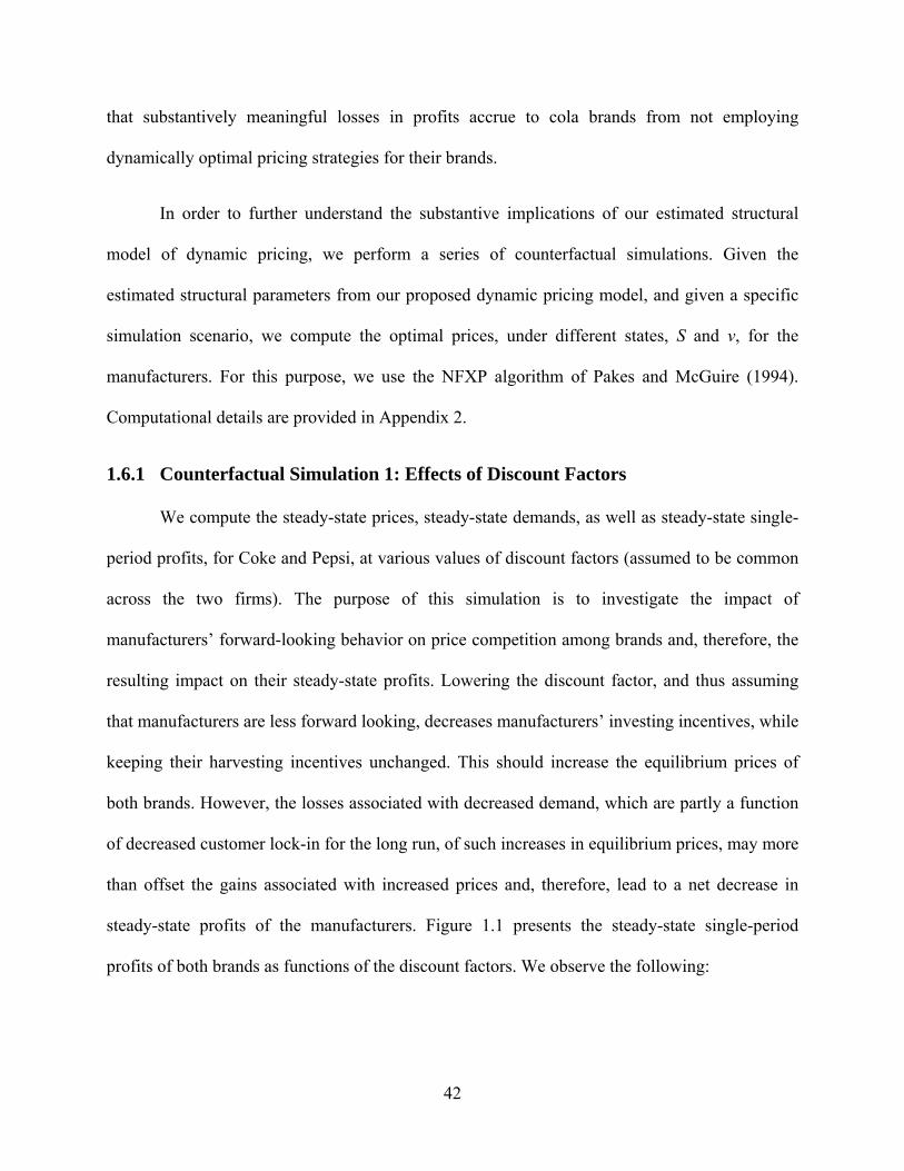
42

that substantively meaningful losses in profits accrue to cola brands from not employing

dynamically optimal pricing strategies for their brands.

In order to further understand the substantive implications of our estimated structural

model of dynamic pricing, we perform a series of counterfactual simulations. Given the

estimated structural parameters from our proposed dynamic pricing model, and given a specific

simulation scenario, we compute the optimal prices, under different states, S and ν, for the

manufacturers. For this purpose, we use the NFXP algorithm of Pakes and McGuire (1994).

Computational details are provided in Appendix 2.

1.6.1 Counterfactual Simulation 1: Effects of Discount Factors

We compute the steady-state prices, steady-state demands, as well as steady-state single-

period profits, for Coke and Pepsi, at various values of discount factors (assumed to be common

across the two firms). The purpose of this simulation is to investigate the impact of

manufacturers’ forward-looking behavior on price competition among brands and, therefore, the

resulting impact on their steady-state profits. Lowering the discount factor, and thus assuming

that manufacturers are less forward looking, decreases manufacturers’ investing incentives, while

keeping their harvesting incentives unchanged. This should increase the equilibrium prices of

both brands. However, the losses associated with decreased demand, which are partly a function

of decreased customer lock-in for the long run, of such increases in equilibrium prices, may more

than offset the gains associated with increased prices and, therefore, lead to a net decrease in

steady-state profits of the manufacturers. Figure 1.1 presents the steady-state single-period

profits of both brands as functions of the discount factors. We observe the following:

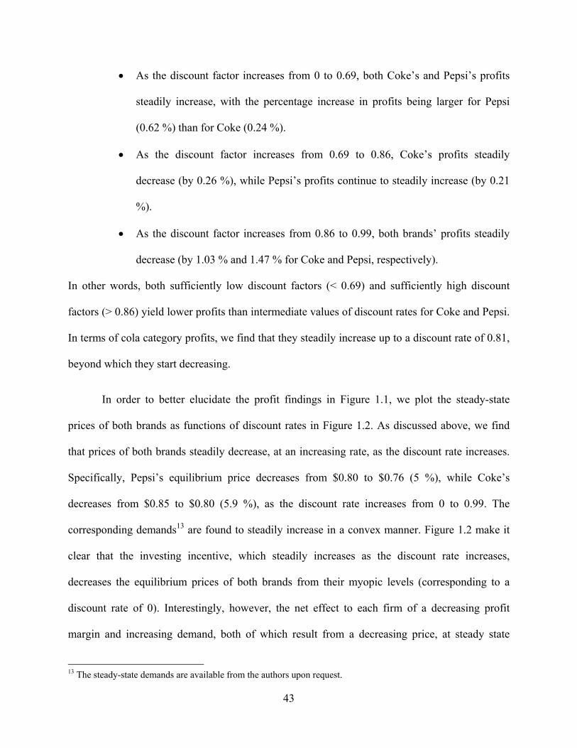
43

As the discount factor increases from 0 to 0.69, both Coke’s and Pepsi’s profits

steadily increase, with the percentage increase in profits being larger for Pepsi

(0.62 %) than for Coke (0.24 %).

As the discount factor increases from 0.69 to 0.86, Coke’s profits steadily

decrease (by 0.26 %), while Pepsi’s profits continue to steadily increase (by 0.21

%).

As the discount factor increases from 0.86 to 0.99, both brands’ profits steadily

decrease (by 1.03 % and 1.47 % for Coke and Pepsi, respectively).

In other words, both sufficiently low discount factors (< 0.69) and sufficiently high discount

factors (> 0.86) yield lower profits than intermediate values of discount rates for Coke and Pepsi.

In terms of cola category profits, we find that they steadily increase up to a discount rate of 0.81,

beyond which they start decreasing.

In order to better elucidate the profit findings in Figure 1.1, we plot the steady-state

prices of both brands as functions of discount rates in Figure 1.2. As discussed above, we find

that prices of both brands steadily decrease, at an increasing rate, as the discount rate increases.

Specifically, Pepsi’s equilibrium price decreases from $0.80 to $0.76 (5 %), while Coke’s

decreases from $0.85 to $0.80 (5.9 %), as the discount rate increases from 0 to 0.99. The

corresponding demands13 are found to steadily increase in a convex manner. Figure 1.2 make it

clear that the investing incentive, which steadily increases as the discount rate increases,

decreases the equilibrium prices of both brands from their myopic levels (corresponding to a

discount rate of 0). Interestingly, however, the net effect to each firm of a decreasing profit

margin and increasing demand, both of which result from a decreasing price, at steady state

13 The steady-state demands are available from the authors upon request.

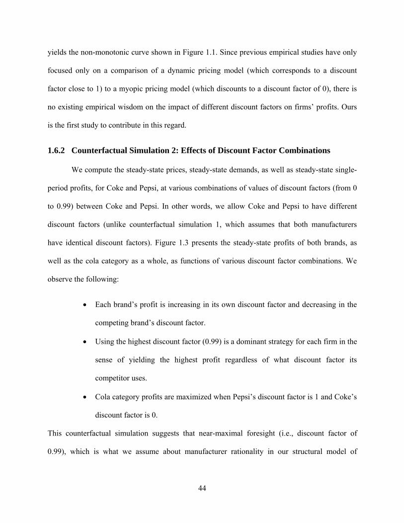
44

yields the non-monotonic curve shown in Figure 1.1. Since previous empirical studies have only

focused only on a comparison of a dynamic pricing model (which corresponds to a discount

factor close to 1) to a myopic pricing model (which discounts to a discount factor of 0), there is

no existing empirical wisdom on the impact of different discount factors on firms’ profits. Ours

is the first study to contribute in this regard.

1.6.2 Counterfactual Simulation 2: Effects of Discount Factor Combinations

We compute the steady-state prices, steady-state demands, as well as steady-state single-

period profits, for Coke and Pepsi, at various combinations of values of discount factors (from 0

to 0.99) between Coke and Pepsi. In other words, we allow Coke and Pepsi to have different

discount factors (unlike counterfactual simulation 1, which assumes that both manufacturers

have identical discount factors). Figure 1.3 presents the steady-state profits of both brands, as

well as the cola category as a whole, as functions of various discount factor combinations. We

observe the following:

Each brand’s profit is increasing in its own discount factor and decreasing in the

competing brand’s discount factor.

Using the highest discount factor (0.99) is a dominant strategy for each firm in the

sense of yielding the highest profit regardless of what discount factor its

competitor uses.

Cola category profits are maximized when Pepsi’s discount factor is 1 and Coke’s

discount factor is 0.

This counterfactual simulation suggests that near-maximal foresight (i.e., discount factor of

0.99), which is what we assume about manufacturer rationality in our structural model of

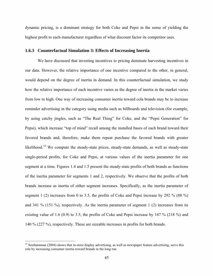
45

dynamic pricing, is a dominant strategy for both Coke and Pepsi in the sense of yielding the

highest profit to each manufacturer regardless of what discount factor its competitor uses.

1.6.3 Counterfactual Simulation 3: Effects of Increasing Inertia

We have discussed that investing incentives to pricing dominate harvesting incentives in

our data. However, the relative importance of one incentive compared to the other, in general,

would depend on the degree of inertia in demand. In this counterfactual simulation, we study

how the relative importance of each incentive varies as the degree of inertia in the market varies

from low to high. One way of increasing consumer inertia toward cola brands may be to increase

reminder advertising in the category using media such as billboards and television (for example,

by using catchy jingles, such as “The Real Thing” for Coke, and the “Pepsi Generation” for

Pepsi), which increase “top of mind” recall among the installed bases of each brand toward their

favored brands and, therefore, make them repeat purchase the favored brands with greater

likelihood.14 We compute the steady-state prices, steady-state demands, as well as steady-state

single-period profits, for Coke and Pepsi, at various values of the inertia parameter for one

segment at a time. Figures 1.4 and 1.5 present the steady-state profits of both brands as functions

of the inertia parameter for segments 1 and 2, respectively. We observe that the profits of both

brands increase as inertia of either segment increases. Specifically, as the inertia parameter of

segment 1 (2) increases from 0 to 3.5, the profits of Coke and Pepsi increase by 292 % (88 %)

and 341 % (151 %), respectively. As the inertia parameter of segment 1 (2) increases from its

existing value of 1.6 (0.9) to 3.5, the profits of Coke and Pepsi increase by 147 % (218 %) and

140 % (227 %), respectively. These are sizeable increases in profits for both brands.

14 Seetharaman (2004) shows that in-store display advertising, as well as newspaper feature advertising, serve this role by increasing consumer inertia toward brands in the long run.

46

In order to better elucidate the profit findings in Figures 1.4 and 1.5, we plot the steady-

state prices of both brands as functions of the inertia parameter for segments 1 and 2,

respectively, in Figures 1.6 and 1.7. We find in both figures that as inertia increases, the price of

each brand steadily decreases -- first at an increasing rate, then linearly, and eventually at a

decreasing rate – until it reaches a minimum and then starts increasing. Specifically, in Figure

1.6 (1.7), Coke’s price decreases from $0.83 ($0.81) to $0.80 ($0.78), i.e., 3.6 % (3.7 %), as the

inertia parameter of segment 1 (2) increases from 0 to 2 (3.5), and then starts increasing. In the

same figure, Pepsi’s price decreases from $0.76 ($0.76) to $0.75 ($0.74), i.e., 1.3 % (2.6 %), as

the inertia parameter of segment 1 (2) increases from 0 to 1 (3), and then starts increasing. This

implies that the investing incentive dominates the harvesting incentive at low and moderate

levels of inertia, while the harvesting incentive dominates the investing incentive at high levels

of inertia.

The steady-state demands for both brands that correspond to the brand prices reflected in

Figure 1.6 and 1.7 are found to steadily increase as the inertia parameter of the respective

segment increases. In order to see how the steady-state demand within each segment behaves, we

separately plot the steady-state demand from each segment in Figures 1.8 and 1.9. Interestingly,

in Figure 1.8 (1.9), we observe monotonically increasing demand from segment 1 (2), but a non-

monotonicity in demand – increasing with inertia, reaching a maximum, and decreasing

thereafter – from segment 2 (1). The non-monotonicity for segment 2 (1) happens at the value of

inertia that corresponds to the non-monotonicity in price that is observed in Figure 1.6 (1.7) for

the same segment. In other words, since the inertia parameter for segment 2 (1) is fixed in Figure

1.8 (1.9), increasing the price of a brand decreases demand for the brand, which is not surprising.

However, the increase in inertia for segment 1 (2) in Figure 1.8 (1.9) overwhelms the increase in

47

price of a brand, when it happens, and sustains the increase in demand for the brand from that

segment over the entire range of inertia tested in this simulation.

48

1.7 Conclusions

In this study, we propose and estimate, for the first time in the literature, a structural

dynamic pricing model in the presence of inertial demand. For this purpose, we study the cola

market, which is characterized by significant inertia in consumers’ brand choices over time. We

estimate a consumer-level brand choice model, which includes the effects of inertia, using

scanner panel data on cola brand choices of consumers in a local market over a period of two

years. We then estimate a manufacturer-level oligopolistic pricing model using retail tracking

data on store-level prices of cola brands from the same local market over the same period of two

years. Using a two-segment brand choice model, we find that the cola category is characterized

by significant inertia in demand, with estimated brand-level switching costs of $0.30 and $0.13

for the two consumer segments. Not accounting for such inertia in brand choices leads to

seriously mis-estimated sensitivities of cola demand to marketing mix variables.

We find that ignoring the investing incentives in manufacturers’ dynamic pricing, as

represented in our dynamic pricing model, leads to a spurious overestimation in the estimated

profit margins of 29 % and 40 % for Coke and Pepsi, respectively. Ignoring both the investing

and harvesting incentives leads to a spurious overestimation in the estimated profit margins of 19

% for both brands. Estimating a mis-specified demand model without inertia and using it as an

input for a static pricing model leads to estimated profit margins that are slightly lower than

those implied by the static pricing model that simply sets the inertia parameter to zero among the

estimated parameters yielded by a demand model with inertia.

The net impact of the harvesting and investing incentives in our data is that the

equilibrium prices of both brands are lower (by 4.6 % and 3.1 % of costs, for Coke and Pepsi,

respectively) than those in the absence of inertia. In other words, the harvesting incentive --

49

which increases equilibrium prices of Coke and Pepsi by 2.3 % and 4.2 %, respectively -- is

dominated by the investing incentive -- which decreases equilibrium prices of Coke and Pepsi by

6.9 % and 7.3 %, respectively -- for cola brands. We find that each brand’s profits would

decrease by about 5 % if it were to engage in myopic pricing while its competitor engages in

dynamic pricing.

A counterfactual simulation reveals that increasing the discount factor from 0 to 1

initially increases, and eventually decreases, the profits of the two brands. Another

counterfactual simulation reveals that each brand’s profits increase in its own discount factor and

decrease in its competitor’s discount factor. A third counterfactual simulation reveals that the

investing incentive to pricing dominates at low to moderate levels of inertia, while the harvesting

incentive dominates at high levels of inertia. However, profits of both brands steadily increase

with inertia.

Some caveats are in order. First, we treat prices an exogenous in our demand model, i.e.,

we do not allow for unobserved demand shocks. We acknowledge that our estimates of marginal

costs may, therefore, be over-estimated if such unobserved demand shocks exist (see Che, Sudhir

and Seetharaman 2007 for a discussion of this issue). Second, our model does not capture an

additional source of dynamics in demand, i.e., due to consumer stockpiling behavior, which has

implications for dynamic pricing. In the cola category, however, stockpiling is not pervasive as

revealed in our data. Households typically buy their preferred quantity of cola on f purchase

occasions. Therefore, ignoring the effects of consumer stockpiling may not be a critical omission

in our case. That said, while extending our model to product categories where consumer

stockpiling is, in fact, significant, explicitly modeling stockpiling behavior, as well as its

implications for dynamic pricing, would be necessary. Third, we ignore the strategic role of the

50

retailer in the analysis. We treat the retailer as a passive intermediary in the distribution channel.

We do this mainly for computational convenience since introducing the dynamic pricing

incentives of the retailer would lead to non-trivial modeling extensions. However, we still obtain

interesting substantive implications from comparing dynamic, myopic, and static pricing

incentives of manufacturers using our framework. Extending our model to additionally

incorporate the strategic role of the retailer is an important area for future research.

We believe that there are some additional research extensions that would be interesting to

pursue. First, investigating the demand conditions under which periodic price promotions of

competing brands emerge as a natural by-product of the competitive dynamic equilibrium in the

presence of inertia would be interesting (see, for example, Freimer and Horsky (2008), for an

interesting analytical model of price promotions in the presence of inertia). Second, extending

the analysis to the case of variety seeking (the opposite of inertia) would be useful to understand

the dynamic pricing implications of variety seeking markets (see, for example, Seetharaman and

Che (2009)). Last, but not least, understanding how to increase inertia in a market to favor one

brand over another would be useful not only in its own research right, but also from the

standpoint of informing brand managers on how to better leverage inertial demand for more

pricing power in the market.

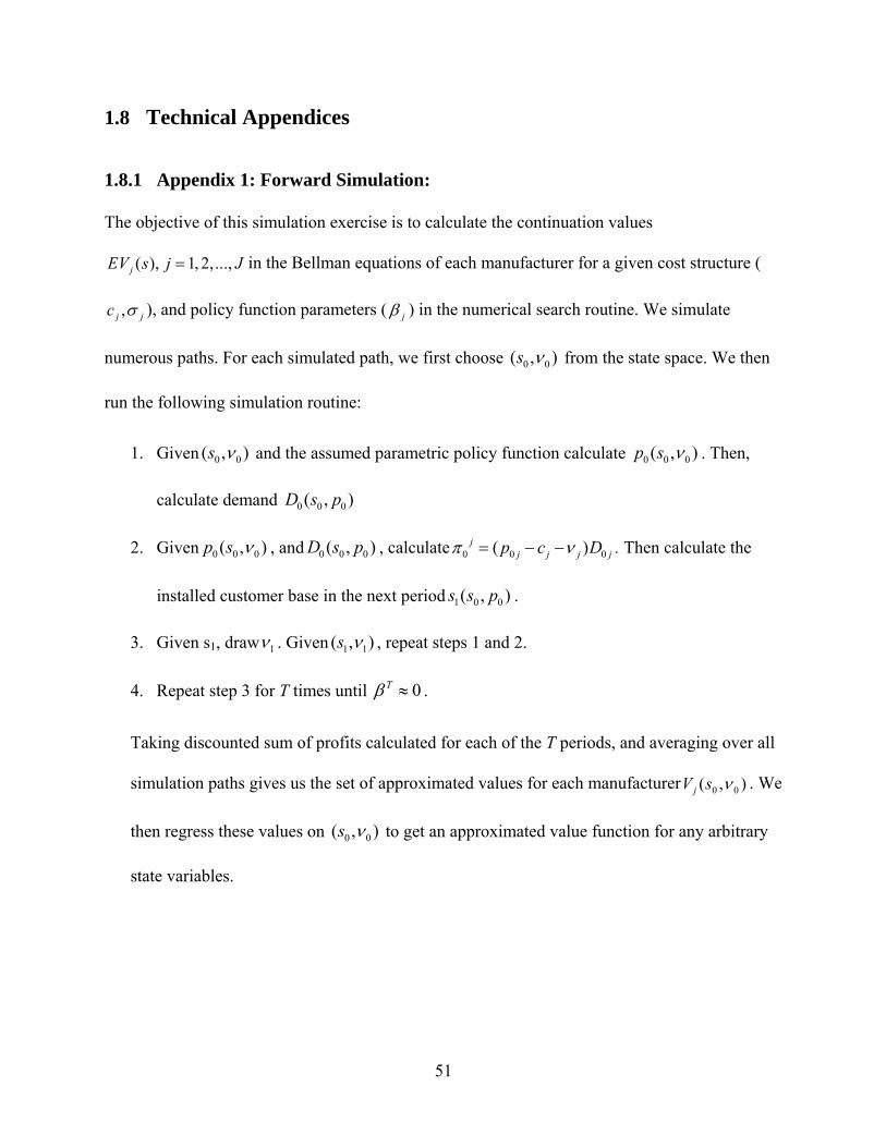
51

1.8 Technical Appendices

1.8.1 Appendix 1: Forward Simulation:

The objective of this simulation exercise is to calculate the continuation values

( ), 1, 2,...,jEV s j J in the Bellman equations of each manufacturer for a given cost structure (

,j jc ), and policy function parameters ( j ) in the numerical search routine. We simulate

numerous paths. For each simulated path, we first choose 0 0( , )s from the state space. We then

run the following simulation routine:

1. Given 0 0( , )s and the assumed parametric policy function calculate 0 0 0( , )p s . Then,

calculate demand 0 0 0( , )D s p

2. Given 0 0 0( , )p s , and 0 0 0( , )D s p , calculate 0 0 0( )jj j j jp c D . Then calculate the

installed customer base in the next period 1 0 0( , )s s p .

3. Given s1, draw 1 . Given 1 1( , )s , repeat steps 1 and 2.

4. Repeat step 3 for T times until 0T .

Taking discounted sum of profits calculated for each of the T periods, and averaging over all

simulation paths gives us the set of approximated values for each manufacturer 0 0( , )jV s . We

then regress these values on 0 0( , )s to get an approximated value function for any arbitrary

state variables.

52

1.8.2 Appendix 2: Multi-Agent NFXP Algorithms for the Counterfactual Studies:

The objective of this routine is to find the dynamic pricing equilibrium of the manufacturer

pricing game numerically. Here is the algorithm:

1. Start with 0 01 2,p p

1.1. Given 02p , get 1

1p by running the subroutine 2.2.

1.2. Given 11p , get 1

2p by running the subroutine 3.4

1.3. Repeat 1.1-1.2 until 1 0n np p .

1.4. Set * np p

Appendix 2.1: Subroutine Coke’s Optimality

The objective of this subroutine is to find the best response of Coke *1p to a given set of actions

of Pepsi 2p , under a given continuation value in Coke’s Bellman equation 1( )EV s . In other

words, the objective is given by

1 1 1 1 1 ' 1arg max ( ) ( ' | , )p p c D E V s s p

where 1D is the demand for Coke. In order to find optimal *1p

1. Start with 01p . Given 0

1p calculate the following:

1 11 1 1 1 11 11

1

( , )( ) ( ')

EV sD p c D EV s

p

where 11 1 1/D D p , and 11 1 1( ( ') / ')( '/ )EV EV s s s p

By rearranging, we can get 11p as follows:

1 11 1 1 1 11 11( ')p c D EV s D

2. Given 11p , repeat step 1, to get 2

1p

3. Repeat step 2 to update 1p until an iteration n such that 11 1 0n np p

4. Set *1 1

np p

Appendix 2.2: Subroutine Coke’s Dynamic Response

53

The objective of this subroutine is to find the dynamic best response of Coke to the set of actions

of Pepsi: 2p . Here is how it goes:

1. Start with 01 ( ) 0EV s : the continuation value is in Coke’s Bellman equation is zero.

a. Get 0*1p under 0

1 ( ) 0EV s by using the subroutine 2.1. Given 0*1 2,p p calculate

the following Bellman equation:

1 0* 0*1 1 1 1 1 ' 1 1 2( , ) ( ) ( ' | , , )V s p c D E V s s p p

b. Given 11 ( , )V s , calculate 1

1 ( )EV s by averaging over . Given 11 ( )EV s get 1*

1p by

using the subroutine 2.1. Calculate the Bellman equation in (a) under 1*1 2,p p .

Calculate the updated continuation value 21 ( )EV s .

c. Repeat (b) until an iteration n such that * 1*1 1 0n np p

d. Set * *1 1

np p

Appendix 2.3: Subroutine Pepsi’s Optimality

The objective of this subroutine is to find the best response of Pepsi *2p to a given set of actions

of Coke 1p , under a given continuation value in Pepsi’s Bellman equation 2 ( )EV s . In other

words, the objective is given by

2 2 2 2 2 ' 2arg max ( ) ( ' | , )p p c D E V s s p

where 2D is the demand for Pepsi. In order to find optimal *2p

1. Start with 02p . Given 0

2p calculate the following:

22 2 2 2 22 22

2

( , )( ) ( ')

V sD p c D EV s

p

where 22 2 2/D D p , and 22 2 2( ( ') / ')( '/ )EV EV s s s p

By rearranging, we can get 12p as follows:

1 12 2 2 2 22 22( ')p c D EV s D

2. Given 12p , repeat step 1, to get 2

2p

3. Repeat step 2 to update 2p until an iteration n such that 12 2 0n np p

54

4. Set *2 2

np p

Appendix 2.4: Subroutine Pepsi’s Dynamic Response

The objective of this subroutine is to find the dynamic best response of Pepsi to the set of actions

of Coke: 1p . Here is how it goes:

1. Start with 02 ( ) 0EV s : the continuation value is in Pepsi’s Bellman equation is zero.

a. Get 0*2p under 0

2 ( ) 0EV s by using the subroutine 2.3. Given 0*1 2,p p

calculate the following Bellman equation:

1 0* 0*2 2 2 2 2 ' 2 1 2( , ) ( ) ( ' | , , )V s p c D E V s s p p

b. Given 12 ( , )V s , calculate 1

2 ( )V s by averaging 12 ( , )V s over . Given

12 ( , )V s get 1*

2p by using the subroutine 2.3. Calculate the Bellman equation

in (a) under 1*1 2,p p . Calculate the updated continuation value 2

2 ( )EV s .

c. Repeat (b) until an iteration n such that * 1*2 2 0n np p

d. Set * *2 2

np p

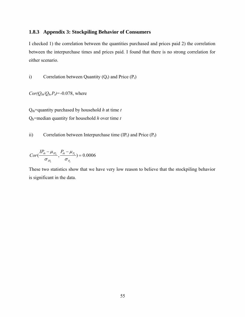
55

1.8.3 Appendix 3: Stockpiling Behavior of Consumers

I checked 1) the correlation between the quantities purchased and prices paid 2) the correlation

between the interpurchase times and prices paid. I found that there is no strong correlation for

either scenario.

i) Correlation between Quantity (Qt) and Price (Pt)

Cor(Qth/Qh,Pt)=-0.078, where

Qth=quantity purchased by household h at time t

Qh=median quantity for household h over time t

ii) Correlation between Interpurchase time (IPt) and Price (Pt)

( , ) 0.0006h h

h h

th IP th P

IP P

IP PCor

These two statistics show that we have very low reason to believe that the stockpiling behavior

is significant in the data.

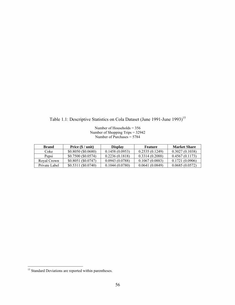
56

Table 1.1: Descriptive Statistics on Cola Dataset (June 1991-June 1993)15

Number of Households = 356 Number of Shopping Trips = 32942

Number of Purchases = 5784

Brand Price ($ / unit) Display Feature Market Share Coke $0.8050 ($0.0680) 0.1458 (0.0953) 0.2535 (0.1249) 0.3027 (0.1038) Pepsi $0.7500 ($0.0574) 0.2236 (0.1818) 0.3314 (0.2088) 0.4567 (0.1173)

Royal Crown $0.8051 ($0.0747) 0.0943 (0.0788) 0.1067 (0.0883) 0.1721 (0.0906) Private Label $0.5311 ($0.0740) 0.1044 (0.0780) 0.0641 (0.0849) 0.0685 (0.0572)

15 Standard Deviations are reported within parentheses.

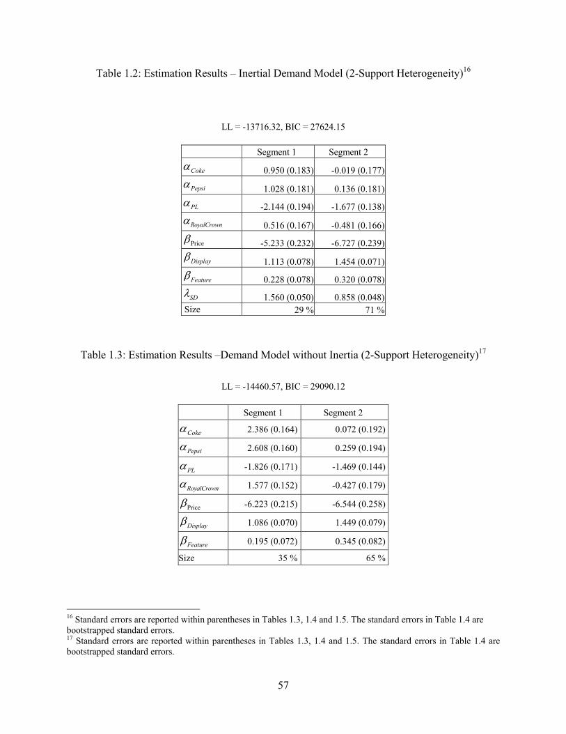
57

Table 1.2: Estimation Results – Inertial Demand Model (2-Support Heterogeneity)16

LL = -13716.32, BIC = 27624.15

Segment 1 Segment 2

Coke 0.950 (0.183) -0.019 (0.177)

Pepsi 1.028 (0.181) 0.136 (0.181)

PL -2.144 (0.194) -1.677 (0.138)

RoyalCrown 0.516 (0.167) -0.481 (0.166)

Price -5.233 (0.232) -6.727 (0.239)

Display 1.113 (0.078) 1.454 (0.071)

Feature 0.228 (0.078) 0.320 (0.078)

SD 1.560 (0.050) 0.858 (0.048) Size 29 % 71 %

Table 1.3: Estimation Results –Demand Model without Inertia (2-Support Heterogeneity)17

LL = -14460.57, BIC = 29090.12

Segment 1 Segment 2

Coke 2.386 (0.164) 0.072 (0.192)

Pepsi 2.608 (0.160) 0.259 (0.194)

PL -1.826 (0.171) -1.469 (0.144)

RoyalCrown 1.577 (0.152) -0.427 (0.179)

Price -6.223 (0.215) -6.544 (0.258)

Display 1.086 (0.070) 1.449 (0.079)

Feature 0.195 (0.072) 0.345 (0.082)

Size 35 % 65 %

16 Standard errors are reported within parentheses in Tables 1.3, 1.4 and 1.5. The standard errors in Table 1.4 are bootstrapped standard errors. 17 Standard errors are reported within parentheses in Tables 1.3, 1.4 and 1.5. The standard errors in Table 1.4 are bootstrapped standard errors.

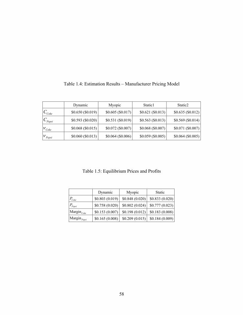
58

Table 1.4: Estimation Results – Manufacturer Pricing Model

Dynamic Myopic Static1 Static2

CokeC $0.650 ($0.019) $0.605 ($0.017) $0.621 ($0.013) $0.635 ($0.012)

PepsiC $0.593 ($0.020) $0.531 ($0.019) $0.563 ($0.013) $0.569 ($0.014)

Coke $0.068 ($0.015) $0.072 ($0.007) $0.068 ($0.007) $0.071 ($0.007)

Pepsi $0.060 ($0.013) $0.064 ($0.006) $0.059 ($0.005) $0.064 ($0.005)

Table 1.5: Equilibrium Prices and Profits

Dynamic Myopic Static

CokeP $0.803 (0.019) $0.848 (0.020) $0.833 (0.020)

PepsiP $0.758 (0.020) $0.802 (0.024) $0.777 (0.023)

MarginCoke $0.153 (0.007) $0.198 (0.012) $0.183 (0.008)

MarginPepsi $0.165 (0.008) $0.209 (0.015) $0.184 (0.009)

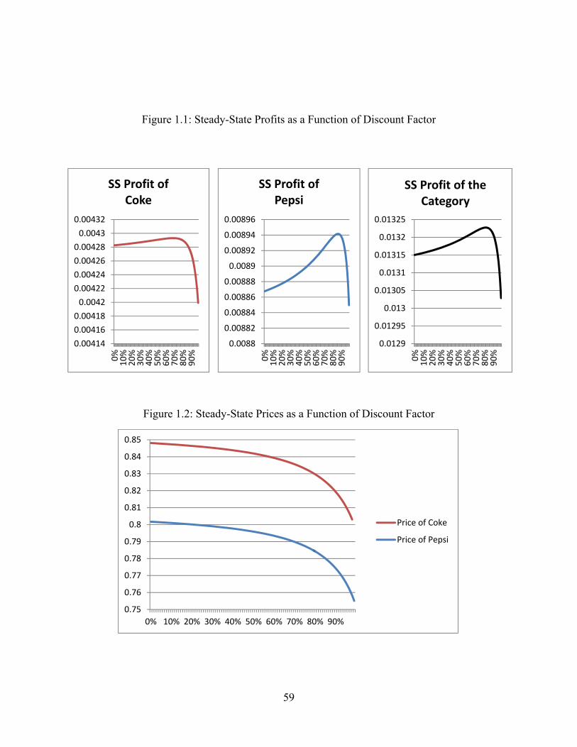
59

Figure 1.1: Steady-State Profits as a Function of Discount Factor

Figure 1.2: Steady-State Prices as a Function of Discount Factor

0.00414

0.00416

0.00418

0.0042

0.00422

0.00424

0.00426

0.00428

0.0043

0.00432

0%

10%

20%

30%

40%

50%

60%

70%

80%

90%

SS Profit of Coke

0.0088

0.00882

0.00884

0.00886

0.00888

0.0089

0.00892

0.00894

0.00896

0%

10%

20%

30%

40%

50%

60%

70%

80%

90%

SS Profit of Pepsi

0.0129

0.01295

0.013

0.01305

0.0131

0.01315

0.0132

0.01325

0%

10%

20%

30%

40%

50%

60%

70%

80%

90%

SS Profit of the Category

0.75

0.76

0.77

0.78

0.79

0.8

0.81

0.82

0.83

0.84

0.85

0% 10% 20% 30% 40% 50% 60% 70% 80% 90%

Price of Coke

Price of Pepsi

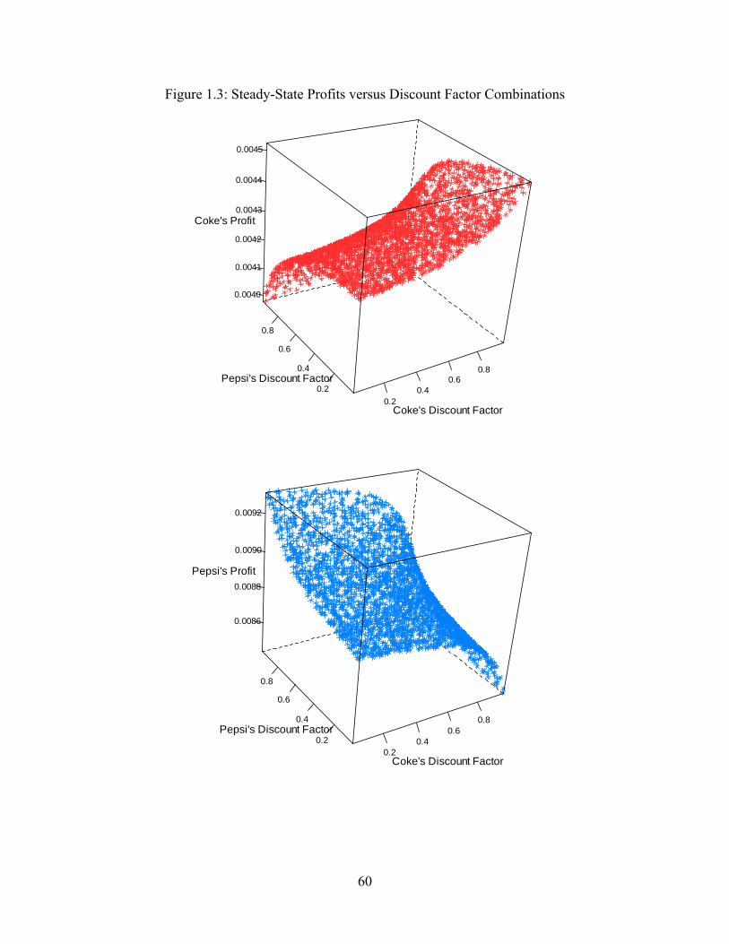
60

Figure 1.3: Steady-State Profits versus Discount Factor Combinations

0.20.4

0.60.8

0.2

0.4

0.6

0.8

0.0040

0.0041

0.0042

0.0043

0.0044

0.0045

Coke's Discount Factor

Pepsi's Discount Factor

Coke's Profit

0.20.4

0.60.8

0.2

0.4

0.6

0.8

0.0086

0.0088

0.0090

0.0092



Pepsi's Profit

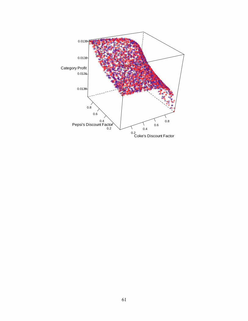
61

0.20.4

0.60.8

0.2

0.4

0.6

0.8

0.0130

0.0131

0.0132

0.0133



Category Profit

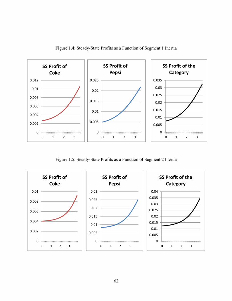
62

Figure 1.4: Steady-State Profits as a Function of Segment 1 Inertia


0

0.002

0.004

0.006

0.008

0.01

0.012

0 1 2 3

SS Profit of Coke

0

0.005

0.01

0.015

0.02

0.025

0 1 2 3

SS Profit of Pepsi

0

0.005

0.01

0.015

0.02

0.025

0.03

0.035

0 1 2 3


0

0.002

0.004

0.006

0.008

0.01

0 1 2 3

SS Profit ofCoke

0

0.005

0.01

0.015

0.02

0.025

0.03

0 1 2 3

SS Profit ofPepsi

0

0.005

0.01

0.015

0.02

0.025

0.03

0.035

0.04

0 1 2 3


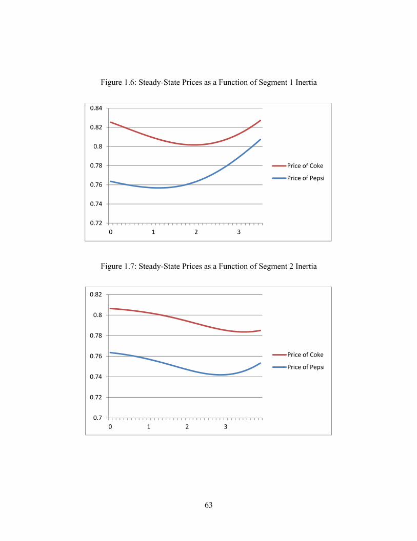
63

Figure 1.6: Steady-State Prices as a Function of Segment 1 Inertia


0.72

0.74

0.76

0.78

0.8

0.82

0.84

0 1 2 3

Price of Coke

Price of Pepsi

0.7

0.72

0.74

0.76

0.78

0.8

0.82

0 1 2 3

Price of Coke

Price of Pepsi

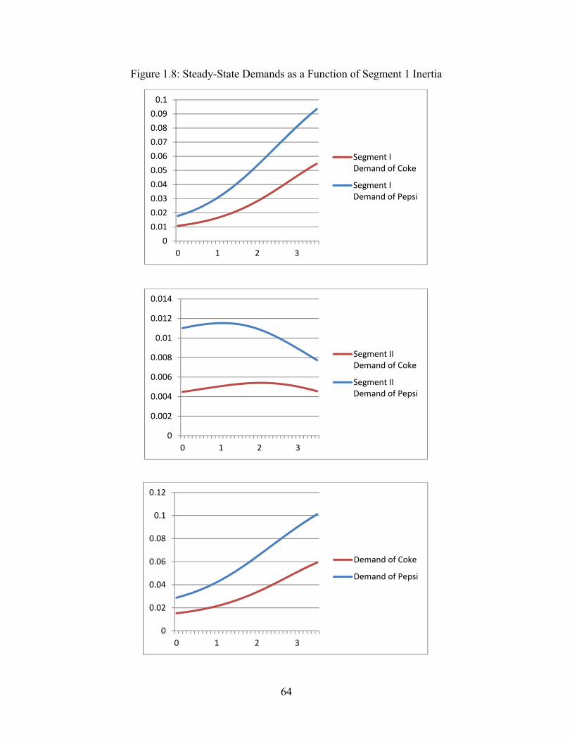
64

Figure 1.8: Steady-State Demands as a Function of Segment 1 Inertia

0

0.01

0.02

0.03

0.04

0.05

0.06

0.07

0.08

0.09

0.1

0 1 2 3

Segment IDemand of Coke

Segment IDemand of Pepsi

0

0.002

0.004

0.006

0.008

0.01

0.012

0.014

0 1 2 3

Segment IIDemand of Coke

Segment IIDemand of Pepsi

0

0.02

0.04

0.06

0.08

0.1

0.12

0 1 2 3

Demand of Coke

Demand of Pepsi

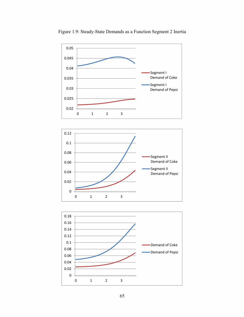
65

Figure 1.9: Steady-State Demands as a Function Segment 2 Inertia

0.02

0.025

0.03

0.035

0.04

0.045

0.05

0 1 2 3

Segment IDemand of Coke

Segment IDemand of Pepsi

0

0.02

0.04

0.06

0.08

0.1

0.12

0 1 2 3



0

0.02

0.04

0.06

0.08

0.1

0.12

0.14

0.16

0.18

0 1 2 3

Demand of Coke

Demand of Pepsi

66

2 Implications of Inertial Demand for Prices in the

Distribution Channel: A Structural Econometric Approach

2.1 Introduction

Consumer product manufacturers, such as Coke and Pepsi, typically sell their brands

through common, independent retailers, such as Kroger. Recent research in the structural

econometric tradition has dealt with the empirical estimation, using real-world scanner data, of

the nature of strategic price interactions in distribution channels, both horizontally among

manufacturers, as well as vertically between manufacturers and the common retailer through

which they sell (see, for example, Kadiyali, Chintagunta and Vilcassim (2000), Sudhir (2001),

Villas-Boas and Zhao (2005), Villas-Boas (2007), Che, Sudhir and Seetharaman (2007),

Draganska, Klapper and Villas-Boas (2010) etc.).18 Such structural econometric models of

pricing in the distribution channel are of great normative value to product manufacturers and

retailers from the standpoint of evaluating and setting optimal pricing policies for their brands

(Bronnenberg, Rossi and Vilcassim (2005)).

It is well documented in the marketing literature that consumer product markets are

commonly characterized by inertia in consumers’ brand choices over time (see, for example,

Seetharaman (2004)).19 Inertia refers to the phenomenon of consumers often repeat-purchasing

the same brand of cola on successive purchase occasions. Such inertial, or habitual, brand choice

behavior of consumers, in turn, leads to the aggregate (e.g., market-level) demand for a brand

being positively correlated over time. In other words, if demand for a brand is high (low) on a 18 The reader is referred to Villas-Boas and Zhao (2005) for an insightful discussion on why it is necessary to jointly consider the strategic behavior of both manufacturers and the retailer while econometrically analyzing retail prices. 19 Economists usually refer to inertia using the term switching costs.

67

given week, it is likely to remain high (low) in ensuing weeks on account of consumer inertia. A

pricing implication of such inertia in demand, for example, is that reducing the retail price of

Coke in the current week will increase the demand for Coke not only in the current week but also

in the subsequent weeks when the price reduction on Coke has been retracted (as long as all

other competing cola brands’ retail prices remain unchanged).

The presence of inertial demand implies that the retailer, while choosing Coke’s retail

price in a given week, would face a trade-off between charging a low price on Coke to attract

customers and locking them in to Coke, versus charging a high price to extract higher profits

from Coke’s already locked-in customers. The retailer faces a similar trade-off while choosing

Pepsi’s retail price in a given week. In sum, therefore, the retailer faces an interesting trade-off in

pricing the cola brand portfolio, for example, in terms of deciding whether to price both Coke

and Pepsi low, versus pricing only Coke (Pepsi) low, versus pricing neither brand low, in a given

week. In order to correctly resolve this trade-off when setting retail prices for cola brands, taking

the manufacturers’ wholesale prices as given, the retailer must know the extent of inertia in

consumers’ brand choices in the cola market, and whether the pricing implications of such inertia

are similar or not among the various brands.

Coca Cola Co. (PepsiCo) must also account for the downstream retailer’s above-

mentioned pricing strategy, as well as its competitor PepsiCo’s (Coca Cola Co.’s) pricing

strategy, both of which, in turn, depend on the degree of inertial demand enjoyed by the cola

brands among consumers, while choosing wholesale prices for their Coke (Pepsi) brand. For

example, suppose Coca Cola Co. knows that the retailer has an incentive to price Coke high in

the current period, in order to harvest the existing demand of past consumers of Coke. In that

case, the manufacturer could then charge higher wholesale prices for Coke to the retailer than

68

otherwise. Conversely, suppose the brand manufacturer knows that the retailer has an incentive

to price Coke low in the current period, in order to invest in increasing the future demand for the

Coke. In this case, the manufacturer must then charge appropriately lower wholesale prices for

Coke to the retailer than otherwise in order to induce the retailer to offer adequately lower retail

prices to the market.

To summarize, therefore, econometrically analyzing the pricing implications of inertial

demand in the context of a distribution channel involves a careful accounting and resolution of

the incentives of competing manufacturers in setting wholesale prices, as well as the incentives

of the common retailer through whom they sell in determining retail prices, for the different

brands in the category. The primary research contribution of our paper rests in our proposal

and estimation of a structural econometric model of dynamic pricing decisions of manufacturers

and a common retailer in the presence of inertia in consumers’ brand choices. Such a model will

be of obvious value to both brand managers and store managers, given the glut of consumer-level

data and analytical tools that are fast permeating the retailing sphere, in guiding strategic pricing

efforts for their brands.

We estimate a consumer-level brand choice model, which includes the effects of inertia,

using scanner panel data on cola brand choices of consumers in a local market over a period of

two years. We then estimate a structural econometric pricing model, that accounts for the pricing

interactions, both among manufacturers, as well as between each manufacturer and the retailer,

using retail tracking data on store-level prices of cola brands from the same local market over

the same period of two years. Using a two-segment brand choice model, we find that the cola

category is characterized by significant inertia in demand, with estimated brand-level switching

costs of $0.30 and $0.13 for the two consumer segments.

69

The net impact of the harvesting and investing incentives for cola manufacturers in our

data is that the equilibrium wholesale prices of both brands are lower (by 11.9 % and 7.1 % of

costs, for Coke and Pepsi, respectively) than those in the absence of inertia. In other words, the

harvesting incentive -- which increases equilibrium wholesale prices of Coke and Pepsi by 5.2 %

and 11.3 %, respectively -- is dominated by the investing incentive -- which decreases

equilibrium wholesale prices of Coke and Pepsi by 17.1 % and 18.4 %, respectively -- for cola

brands. For the retailer, however, while the harvesting incentive increases the retailer’s profit

margin by 1.9c and 2.5c, the investing incentive has no impact on retail profit margin. In other

words, while the retailer exploits the benefit of the harvesting incentive, by appropriately

increasing his retail profit margin, almost equally with the manufacturers, the cost of investing is

borne entirely by the manufacturers. In other words, the retailer effectively free rides on the


from the existence of inertial demand. In terms of the net effect of the harvesting and investing

incentives on distribution channel profits, we uncover a 3c lowered channel profit margin for

Coke, but no change in the channel profit margin for Pepsi.

Using the estimates of our structural econometric model, we study the impact of inertial

demand on the estimated profitability of the retailer and each manufacturer using two

counterfactual simulations. In the first counterfactual simulation, we study the impact of

increasing inertia on each channel member’s profits and investigate which player in the

distribution channel – manufacturer or retailer -- is in a better position to leverage the benefits of

inertial demand in terms of gaining disproportionately more from, say, increasing levels of

inertia in the market. We find that all channel members gain from increasing levels of inertia,

with the retailer gaining disproportionately more than the manufacturers. The investing incentive

70

becomes more important for manufacturers as the level of inertia in either consumer segment

increases, thus leading to lower wholesale profit margins. However, as far as the retailer is

concerned, an interesting asymmetry emerges. As the level of inertia in the less inertial segment

increases, the investing incentive becomes more important to the retailer, thus leading to lower

retail profit margins, although at a slower rate than for the manufacturers. However, as the level

of inertia in the more inertial segment increases, the retailer not only does not bear the costs of

the investing incentive (while the manufacturers do), but also ends up free-riding on the

manufacturers’ efforts by steadily increasing his retail profit margins on both brands. This

simulation suggests that the retailer is in a more leveraged position of strength when it comes to

exploiting the increase in inertial demand for cola brands in either consumer segment.

In the second counterfactual simulation, we study the benefits of behavioral price

discrimination, using price-off coupons that are customized across behavioral segments of

consumers, for the retailer and the manufacturers. We find that the retailer can improve retail

profit by 4 % by dropping customized coupons to customers belonging to the more price-

sensitive / less inertial segment. Interestingly, we find that the retailer can improve retail profit

by an additional 7 % by selling its customer database to both cola manufacturers and letting them

drop customized coupons for their brands to customers belonging to segment 2, as opposed to

dropping the customized coupons itself. In other words, facilitating manufacturer couponing is a

more profitable strategy to the retailer than undertaking store couponing itself. Interestingly, this

leads to both manufacturers being slightly worse off, in terms of reduced wholesale profits, when

compared to the case of no price discrimination. In other words, the retailer not only entirely

benefits at the expense of manufacturers, but also induces the manufacturers to invest the

necessary effort to generate the additional channel profits.

71

2.2 Literature Review

There are two seminal game-theoretic studies, namely Beggs and Klemperer (1992) and

Wernerfelt (1991), that centrally motivate the importance of our econometric research from the

standpoint of pricing strategies of brand manufacturers. We discuss these two studies first, and

later studies on the same issue next.

Beggs and Klemperer (1992) derive the normative pricing implications of inertial

demand in a differentiated duopoly using an infinite period game-theoretic framework, where

new customers arrive and a fraction of old consumers leave in each period. Furthermore, in each

period, old (locked-in) customers and new (uncommitted) customers are intermingled and the

two firms cannot discriminate between these groups of customers. The authors study whether the

firms’ temptation to exploit their current customer bases would lead to higher prices (harvesting

incentive), or whether the firms’ desire to attract new customers would lead to lower prices

(investing incentive), than in the case of no inertia. The authors show that under a wide range of

parametric assumptions, both firms – each with an installed base of existing customers – face

demand functions that are relatively price inelastic compared to their counterparts in an

otherwise identical mature market without inertia. This decreased price elasticity reduces the

price rivalry among the firms, leading to higher prices and profits for both firms. The authors

show that inertial demand could lead to vigorous price competition in the early growth stages of

a market, as competing firms aggressively try to build market shares for their brands. When the

modeling framework allows for rational (i.e., “forward-looking”) consumers, the prices of the

two firms are shown to become less competitive because consumers who realize that firms with

higher market shares will charge higher prices in the future are less price elastic than naïve

consumers. The authors find that price rise as (1) firms discount the future more, (2) consumers

72

discount the future less, (3) turnover of consumers decreases, and (4) the rate of growth of the

market decreases.

In contrast to the discrete-time, game-theoretic framework adopted by Beggs and

Klemperer (1992), Wernerfelt (1991) adopts a continuous-time, game-theoretic framework to

study price competition between firms in inertial markets. Consistent with the findings in Beggs

and Klemperer (1992), Wernerfelt (1991) also derives higher equilibrium prices for firms, as

well as a positive effect of the extent of firms’ future discounting behavior on equilibrium prices,

in inertial markets. This shows that the equilibrium pricing results are robust to whether the

game-theoretic pricing models are solved in discrete or continuous time.

Unlike Beggs and Klemperer (1992) and Wernerfelt (1991), who show that the

harvesting incentive outweighs the investing incentive for manufacturers under a wide range of

parametric assumptions, Chintagunta and Rao (1996) and Dube, Hitsch and Rossi (2009) find the

opposite to be the case under some parametric assumptions that are based on actual demand

estimates. They show that myopic pricing strategies of firms that fail to recognize the long-run

impact of their current prices lead to prices that are higher than those implied by dynamic pricing

strategies. Doganoglu (2010) obtains the same result when the degree of inertia in demand in his

model is assumed to be sufficiently low. Villas-Boas (2004) also derives the same result for the

case where inertial demand endogenously arises out of consumers learning about how well

different brands fit their preferences, and when the distribution of consumer valuations for each

product is negatively skewed. In a recent study, Cosguner, Chan and Seetharaman (2012) obtain

the same result by actually estimating an econometric model of oligopolistic manufacturer

pricing using retail price data.

73

All of the models of dynamic pricing discussed above ignore the strategic role of the

retailer in the distribution channel. In other words, the pricing implications of inertial demand are

derived for manufacturer pricing, tacitly assuming that manufacturers sell directly to end

consumers. Two recent studies look at the consequences of inertial demand for retailers’ pricing

decisions, namely, Che, Sudhir and Seetharaman (2007) and Dube, Hitsch, Rossi and Vitorino

(2009). However, Dube et al. (2009) derive optimal retailer prices, ignoring the role of

manufacturers and, therefore, treating the retailer’s costs as exogenously specified. Che et al.

(2007), on the other hand, simultaneously account for the strategic role of competing

manufacturers in setting wholesale prices, while deriving optimal retail prices in the distribution

channel. Furthermore, Che et al. (2009) take an econometric, as opposed to a purely game-

theoretic, approach in explaining retail pricing decisions of retailers. In this sense, the Che et al.

(2007) study is closely related to this research. However, given the computational challenges

associated with the estimation of a structural econometric model of pricing in the distribution

channel (as will be explained in the next paragraph), Che et al. (2007) formulate their pricing

model for a finite number of decision periods only (as opposed to infinite periods). Our study

relaxes this restrictive assumption and derives the appropriate pricing model for the distribution

channel under the general case of infinite period decision-making of manufacturers (as in the

game-theoretic literature, see, for example, Beggs and Klemperer (1992) and Wernerfelt (1991)),

as well as the retailer. In doing this, we are able to understand the tension between the harvesting

and investing incentives of manufacturers and the retailer in driving the observed retail prices of

brands in our data. More generally, our approach can be used by manufacturers and retailers in

order to correctly assess the long-run consequences of alternative pricing strategies of brands,

something that cannot be satisfactorily accomplished using the Che et al. (2007) approach.20 20 Che et al. (2007) represent a pioneering effort in the estimation of dynamic pricing decisions of manufacturers and

74

Estimable econometric models of dynamic pricing in the distribution channel in the

presence of inertial demand require both (1) the solution of discrete-time, stochastic dynamic

optimization problems for each manufacturer and retailer, where the manufacturer (retailer)

chooses from a continuum of possible wholesale (retail) prices, and (2) the fixed point to the

game-theoretic problem of multiple firms (manufacturers and retailer) employing their best

pricing responses to each other’s pricing choices, to be accommodated in the estimation. Such

models, referred to as structural models of dynamic pricing in the distribution channel in the

presence of inertial demand, therefore, present significant computational challenges. An

additional estimation challenge arises when some firm actions (such as wholesale prices, as in

our case) are unobserved by the researcher. In fact, as we will discuss in detail later, this

difficulty renders recently developed econometric techniques in the econometrics literature –

Pakes and McGuire (2001), Bajari, Benkard and Levin (2007) etc. – inapplicable to our context.

We propose a fully dynamic pricing model for the distribution channel, as well as a new

estimation method to recover its parameters when some of the agents’ actions are unobserved.

We apply our structural econometric model of dynamic pricing in the distribution channel to the

cola market.

The rest of the paper is organized as follows. In the next section, we present our structural

econometric model of inertial demand, as well as the associated estimation procedure. In the

third section, we present our structural econometric model of dynamic pricing in the distribution

channel in the presence of inertial demand, as well as the associated estimation procedure.

Section 4 presents the estimation results from applying our proposed structural econometric

models of inertial demand and dynamic distribution channel pricing on scanner panel data from

the retailer in the presence of inertial demand. Our effort represents a logical next step given the computational advances of recent years.

75

the cola market. In Section 5, we discuss the managerial implications of our estimation results

based on some counterfactual simulations, one of which pertains to behavioral price

discrimination. Section 6 concludes with caveats and directions for future research.

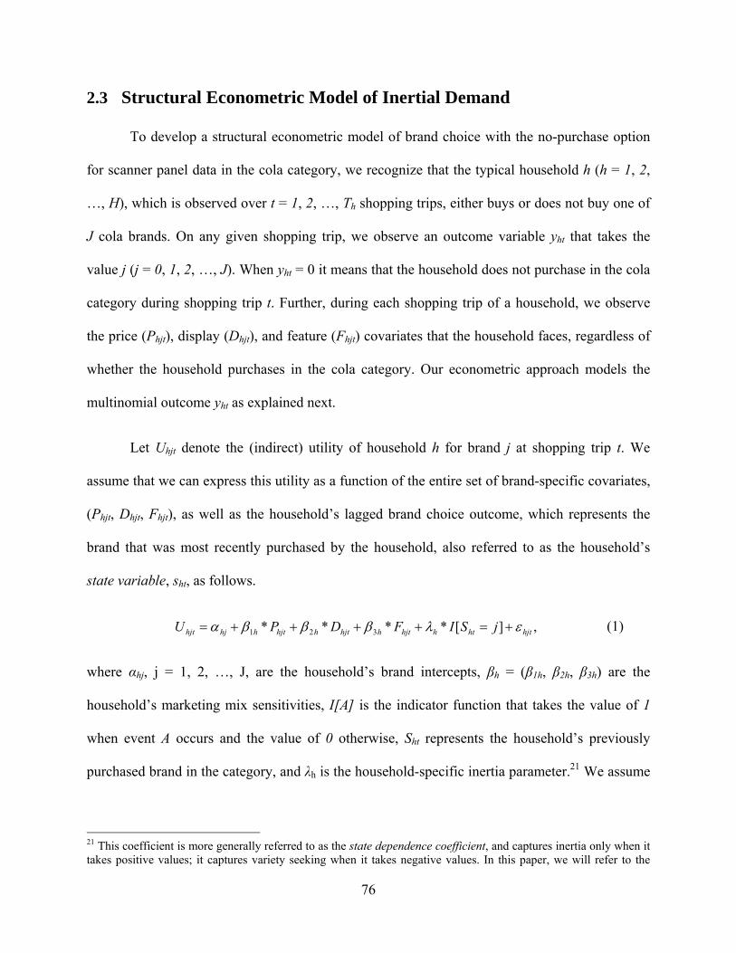
76

2.3 Structural Econometric Model of Inertial Demand

To develop a structural econometric model of brand choice with the no-purchase option

for scanner panel data in the cola category, we recognize that the typical household h (h = 1, 2,

…, H), which is observed over t = 1, 2, …, Th shopping trips, either buys or does not buy one of

J cola brands. On any given shopping trip, we observe an outcome variable yht that takes the

value j (j = 0, 1, 2, …, J). When yht = 0 it means that the household does not purchase in the cola

category during shopping trip t. Further, during each shopping trip of a household, we observe

the price (Phjt), display (Dhjt), and feature (Fhjt) covariates that the household faces, regardless of

whether the household purchases in the cola category. Our econometric approach models the

multinomial outcome yht as explained next.

Let Uhjt denote the (indirect) utility of household h for brand j at shopping trip t. We

assume that we can express this utility as a function of the entire set of brand-specific covariates,

(Phjt, Dhjt, Fhjt), as well as the household’s lagged brand choice outcome, which represents the

brand that was most recently purchased by the household, also referred to as the household’s

state variable, sht, as follows.

1 2 3* * * * [ ] ,hjt hj h hjt h hjt h hjt h ht hjtU P D F I S j (1)

where αhj, j = 1, 2, …, J, are the household’s brand intercepts, βh = (β1h, β2h, β3h) are the

household’s marketing mix sensitivities, I[A] is the indicator function that takes the value of 1

when event A occurs and the value of 0 otherwise, Sht represents the household’s previously

purchased brand in the category, and λh is the household-specific inertia parameter.21 We assume

21 This coefficient is more generally referred to as the state dependence coefficient, and captures inertia only when it takes positive values; it captures variety seeking when it takes negative values. In this paper, we will refer to the

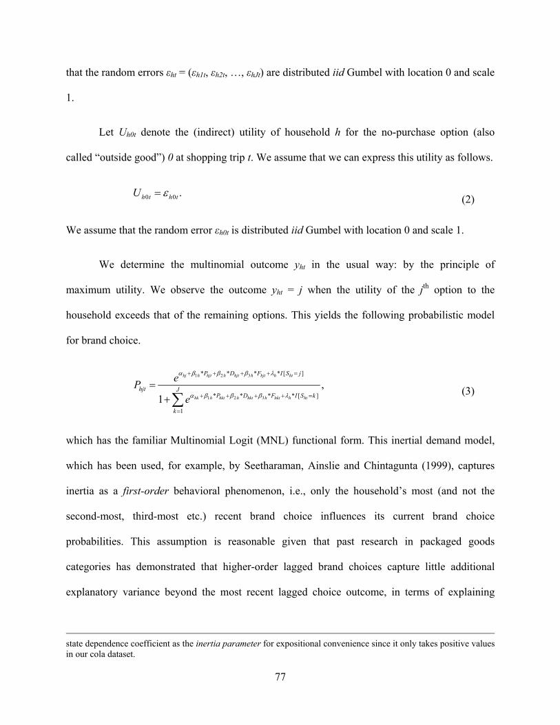
77

that the random errors εht = (εh1t, εh2t, …, εhJt) are distributed iid Gumbel with location 0 and scale

1.

Let Uh0t denote the (indirect) utility of household h for the no-purchase option (also

called “outside good”) 0 at shopping trip t. We assume that we can express this utility as follows.

0 0 .h t h tU (2)

We assume that the random error εh0t is distributed iid Gumbel with location 0 and scale 1.

We determine the multinomial outcome yht in the usual way: by the principle of

maximum utility. We observe the outcome yht = j when the utility of the jth option to the

household exceeds that of the remaining options. This yields the following probabilistic model

for brand choice.

1 2 3

1 2 3

* * * * [ ]

* * * * [ ]

1

,1

hj h hjt h hjt h hjt h ht

hk h hkt h hkt h hkt h ht

P D F I S j

hjt JP D F I S k

k

eP

e

(3)

which has the familiar Multinomial Logit (MNL) functional form. This inertial demand model,

which has been used, for example, by Seetharaman, Ainslie and Chintagunta (1999), captures

inertia as a first-order behavioral phenomenon, i.e., only the household’s most (and not the

second-most, third-most etc.) recent brand choice influences its current brand choice

probabilities. This assumption is reasonable given that past research in packaged goods

categories has demonstrated that higher-order lagged brand choices capture little additional

explanatory variance beyond the most recent lagged choice outcome, in terms of explaining

state dependence coefficient as the inertia parameter for expositional convenience since it only takes positive values in our cola dataset.

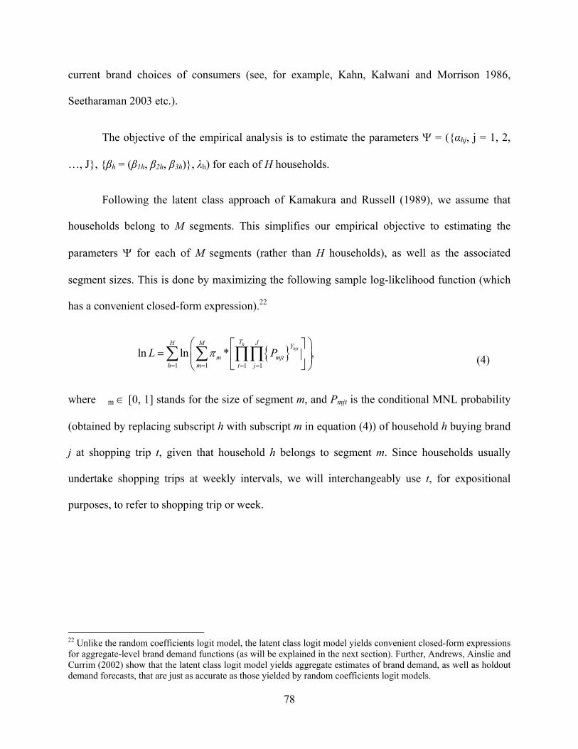
78

current brand choices of consumers (see, for example, Kahn, Kalwani and Morrison 1986,

Seetharaman 2003 etc.).

The objective of the empirical analysis is to estimate the parameters = ({αhj, j = 1, 2,

…, J}, {βh = (β1h, β2h, β3h)}, λh) for each of H households.

Following the latent class approach of Kamakura and Russell (1989), we assume that

households belong to M segments. This simplifies our empirical objective to estimating the

parameters for each of M segments (rather than H households), as well as the associated

segment sizes. This is done by maximizing the following sample log-likelihood function (which

has a convenient closed-form expression).22

1 1 1 1

ln ln * ,h

hjtT JH M Y

m mjth m t j

L P

(4)

where �m [0, 1] stands for the size of segment m, and Pmjt is the conditional MNL probability

(obtained by replacing subscript h with subscript m in equation (4)) of household h buying brand

j at shopping trip t, given that household h belongs to segment m. Since households usually

undertake shopping trips at weekly intervals, we will interchangeably use t, for expositional

purposes, to refer to shopping trip or week.

22 Unlike the random coefficients logit model, the latent class logit model yields convenient closed-form expressions for aggregate-level brand demand functions (as will be explained in the next section). Further, Andrews, Ainslie and Currim (2002) show that the latent class logit model yields aggregate estimates of brand demand, as well as holdout demand forecasts, that are just as accurate as those yielded by random coefficients logit models.

79

2.4 Structural Econometric Model of Dynamic Distribution Channel

Pricing in the Presence of Inertial Demand

To develop a structural econometric model of distribution channel pricing in the cola

category, we recognize that each manufacturer j (j = Coke, Pepsi) sets a wholesale price for a

retailer, while the retailer then sets a retail price, for their brand, during each of t = 1, 2, …, T

weeks in the data.23 The retailer is a monopolist in a local market. During each week, we observe

an outcome variable Pjt > 0 for each brand. Our econometric approach models the continuous

outcome Pjt as explained next. We do this in two steps. We first derive a predictive model of

aggregate-level brand demand, which is an aggregation of individual-level brand demand, as

derived in the previous section. We then embed this predictive model of aggregate-level brand

demand within a dynamic pricing game within a distribution channel involving competing

manufacturers and a common retailer. This dynamic pricing game assumes that manufacturers

engage in Bertrand price competition with each other while setting their wholesale prices, while

the retailer plays the role of a Stackelberg follower while setting retail prices for the

manufacturers’ brands (taking their wholesale prices as given).

2.4.1 Predictive Model of Aggregate-Level Brand Demand

Let Sjtm denote a state variable that represents the (segment-specific) installed base for

brand j during week t. This installed base variable represents the number of consumers in

segment m, as of week t, whose most recent brand choice in the cola category is brand j. Further,

let 1 2( , ,..., )m m m mt t t JtS S S S represent the vector of installed base variables across all J brands during

23 While there are 4 brands – Coke, Pepsi, Royal Crown, and Private Label – in the cola category, we endogenize the prices of only the two major brands – Coke, Pepsi – in the empirical analysis. This is done for computational convenience. The prices of Royal Crown and Private Label are treated as exogenous to the analysis.

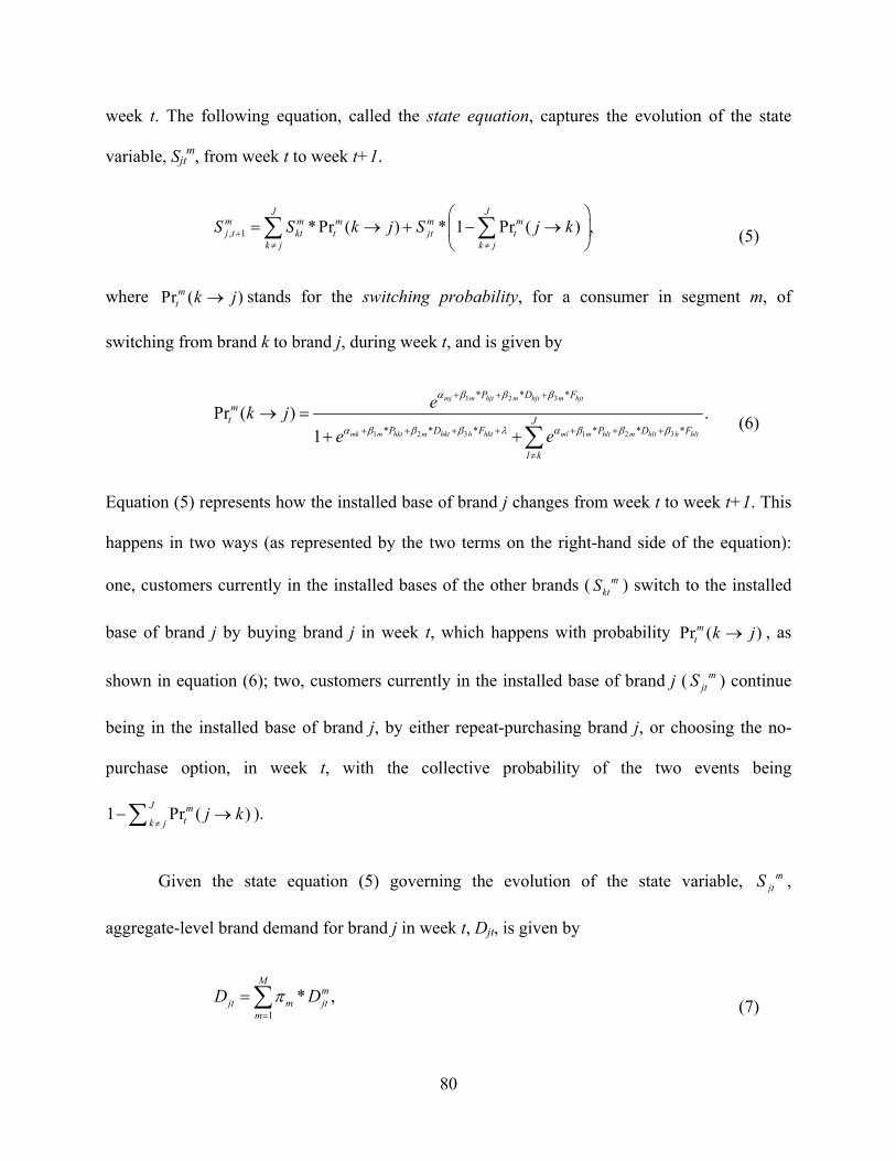
80

week t. The following equation, called the state equation, captures the evolution of the state

variable, Sjtm, from week t to week t+1.

, 1 * Pr ( ) * 1 Pr ( ) ,J J

m m m m mj t kt t jt t

k j k j

S S k j S j k

(5)

where Pr ( )mt k j stands for the switching probability, for a consumer in segment m, of

switching from brand k to brand j, during week t, and is given by

1 2 3

1 2 3 1 2 3

* * *

* * * * * *

Pr ( ) .1

mj m hjt m hjt m hjt

mk m hkt m hkt h hkt ml m hlt m hlt h hlt

P D Fm

t JP D F P D F

l k

ek j

e e

(6)

Equation (5) represents how the installed base of brand j changes from week t to week t+1. This

happens in two ways (as represented by the two terms on the right-hand side of the equation):

one, customers currently in the installed bases of the other brands ( mktS ) switch to the installed

base of brand j by buying brand j in week t, which happens with probability Pr ( )mt k j , as

shown in equation (6); two, customers currently in the installed base of brand j ( mjtS ) continue

being in the installed base of brand j, by either repeat-purchasing brand j, or choosing the no-

purchase option, in week t, with the collective probability of the two events being

1 Pr ( )J m

tk jj k

).

Given the state equation (5) governing the evolution of the state variable, mjtS ,

aggregate-level brand demand for brand j in week t, Djt, is given by

1

* ,M

mjt m jt

m

D D

(7)

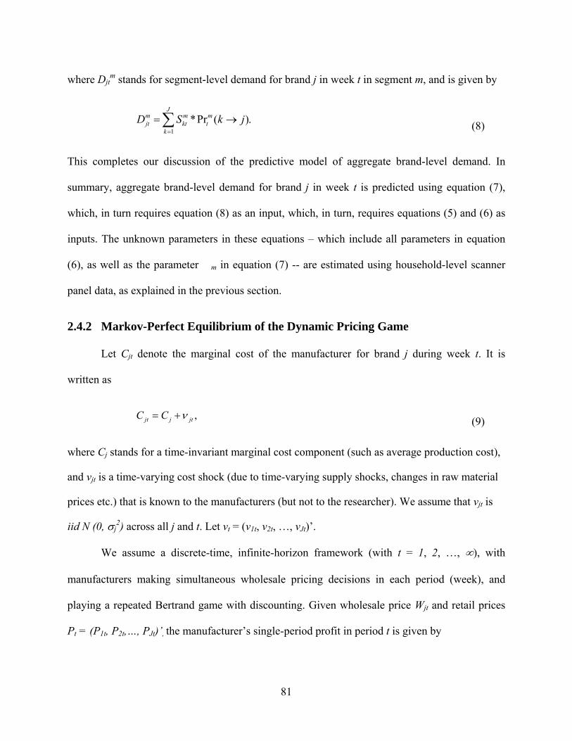
81

where Djtm stands for segment-level demand for brand j in week t in segment m, and is given by

1

*Pr ( ).J

m m mjt kt t

k

D S k j

(8)

This completes our discussion of the predictive model of aggregate brand-level demand. In

summary, aggregate brand-level demand for brand j in week t is predicted using equation (7),

which, in turn requires equation (8) as an input, which, in turn, requires equations (5) and (6) as

inputs. The unknown parameters in these equations – which include all parameters in equation

(6), as well as the parameter �m in equation (7) -- are estimated using household-level scanner

panel data, as explained in the previous section.

2.4.2 Markov-Perfect Equilibrium of the Dynamic Pricing Game

Let Cjt denote the marginal cost of the manufacturer for brand j during week t. It is

written as

,jt j jtC C (9)

where Cj stands for a time-invariant marginal cost component (such as average production cost),

and νjt is a time-varying cost shock (due to time-varying supply shocks, changes in raw material

prices etc.) that is known to the manufacturers (but not to the researcher). We assume that νjt is

iid N (0, j2) across all j and t. Let νt = (ν1t, ν2t, …, νJt)’.

We assume a discrete-time, infinite-horizon framework (with t = 1, 2, …, ), with

manufacturers making simultaneous wholesale pricing decisions in each period (week), and

playing a repeated Bertrand game with discounting. Given wholesale price Wjt and retail prices

Pt = (P1t, P2t,…, PJt)’, the manufacturer’s single-period profit in period t is given by

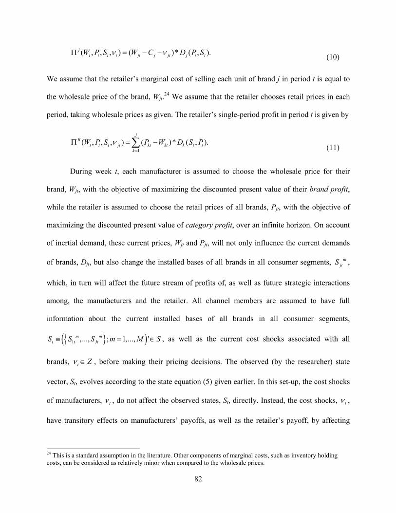
82

( , , , ) ( )* ( , ).jt t t t jt j jt j t tW P S W C D P S

(10)

We assume that the retailer’s marginal cost of selling each unit of brand j in period t is equal to

the wholesale price of the brand, Wjt.24 We assume that the retailer chooses retail prices in each

period, taking wholesale prices as given. The retailer’s single-period profit in period t is given by

1

( , , , ) ( )* ( , ).J

Rt t t jt kt kt k t t

k

W P S P W D S P

(11)

During week t, each manufacturer is assumed to choose the wholesale price for their

brand, Wjt, with the objective of maximizing the discounted present value of their brand profit,

while the retailer is assumed to choose the retail prices of all brands, Pjt, with the objective of

maximizing the discounted present value of category profit, over an infinite horizon. On account

of inertial demand, these current prices, Wjt and Pjt, will not only influence the current demands

of brands, Djt, but also change the installed bases of all brands in all consumer segments, mjtS ,

which, in turn will affect the future stream of profits of, as well as future strategic interactions

among, the manufacturers and the retailer. All channel members are assumed to have full

information about the current installed bases of all brands in all consumer segments,

1 ,..., ; 1,..., 'm mt t JtS S S m M S , as well as the current cost shocks associated with all

brands, t Z , before making their pricing decisions. The observed (by the researcher) state

vector, St, evolves according to the state equation (5) given earlier. In this set-up, the cost shocks

of manufacturers, t , do not affect the observed states, St, directly. Instead, the cost shocks, t ,

have transitory effects on manufacturers’ payoffs, as well as the retailer’s payoff, by affecting

24 This is a standard assumption in the literature. Other components of marginal costs, such as inventory holding costs, can be considered as relatively minor when compared to the wholesale prices.

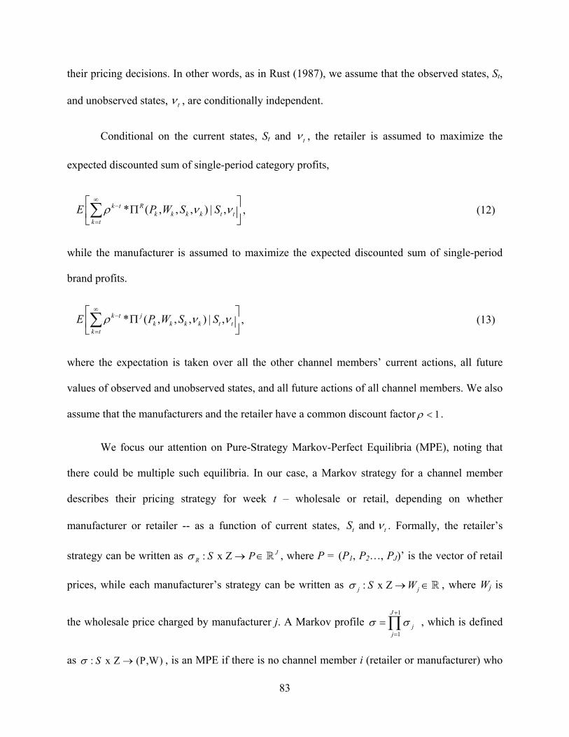
83

their pricing decisions. In other words, as in Rust (1987), we assume that the observed states, St,

and unobserved states, t , are conditionally independent.

Conditional on the current states, St and t , the retailer is assumed to maximize the

expected discounted sum of single-period category profits,

* ( , , , ) | ,k t Rk k k k t t

k t

E P W S S

, (12)

while the manufacturer is assumed to maximize the expected discounted sum of single-period

brand profits.

* ( , , , ) | ,k t jk k k k t t

k t

E P W S S

, (13)

where the expectation is taken over all the other channel members’ current actions, all future

values of observed and unobserved states, and all future actions of all channel members. We also

assume that the manufacturers and the retailer have a common discount factor 1 .

We focus our attention on Pure-Strategy Markov-Perfect Equilibria (MPE), noting that

there could be multiple such equilibria. In our case, a Markov strategy for a channel member

describes their pricing strategy for week t – wholesale or retail, depending on whether

manufacturer or retailer -- as a function of current states, and t tS . Formally, the retailer’s

strategy can be written as : x Z JR S P , where P = (P1, P2…, PJ)’ is the vector of retail

prices, while each manufacturer’s strategy can be written as : x Zj jS W , where Wj is

the wholesale price charged by manufacturer j. A Markov profile 1

1

J

jj

, which is defined

as : x Z (P,W)S , is an MPE if there is no channel member i (retailer or manufacturer) who

84

prefers an alternative strategy 'i over i , when all other channel members are choosing their

strategies according to i . This can be formally written as follows.

( , | , ) ( , | ', ), , , ',i i i i i i iV S V S i S (14)

Given that the behavior is a Markov profile, for each manufacturer j, the discounted sum

of profits can be written in the form of the following Bellman equation.

( , ) sup ( )* ( , ) * ( ' | , ) ( ')jj W j j j j jV S W C D S P V S S P dF , (15)

Similarly, the retailer’s discounted sum of profits can be written as the form of the following

Bellman equation.

1 2, ,...,1

( , ) sup ( )* ( , ) * ( ' | , ) ( ') .J

J

R P P P k k k Rk

V S P W D S P V S S P dF

(16)

It is useful to note that the payoff relevant states for the retailer are (S, ), which are identical to

those for each manufacturer. While the retailer’s pricing decisions are directly influenced only by

manufacturers’ wholesale prices, since the manufacturers’ wholesale prices are functions of S

and , the value function of the retailer is a function of (S, ).

2.4.3 Estimation Challenges

The objective of the estimation is to estimate the parameters ({Cj, �j} j = 1, 2, …, J}).

The biggest challenge for the researcher is that wholesale prices are unobserved, but as

manufacturers’ wholesale pricing policies will determine the retailer’s retail pricing policy, if the

retailer’s continuation value in equation (16) is known, under the Stackelberg assumption, one

can invert unobserved wholesale prices by using the retailer’s optimality conditions for setting

retail prices. Similarly, if each manufacturer’s continuation value in equation (15) is known,

85

under the Bertrand assumption, one can invert unobserved manufacturer costs by using the

manufacturer’s optimality conditions for setting wholesale prices. Thereafter, putting the

retailer’s and manufacturers’ value functions together, and by jointly exploiting the optimality

conditions of the retailer and the manufacturer (which gets rid of the unobserved wholesale

prices since they cancel out), one can infer the marginal costs of the manufacturers using

observed retail prices. This estimation strategy is adopted in Sudhir (2001). Such a strategy is

facilitated by the authors’ assumptions that there are no unobserved structural cost shocks for

manufacturers, and that the channel members maximize their profits over a finite number (i.e.,

three) of periods. Neither assumption holds in our case. We allow for structural cost shocks, ,

as well as assume that manufacturers and the retailer maximize infinite-period expected profits.

This results in the value functions of the retailer and the manufacturers not having a closed form

in our case, which makes the estimation strategy of Sudhir (2001) inapplicable.

Since the continuation values in equations (15) and (16) are not known, one needs to

compute the continuation values of the dynamic game for each candidate cost structure. There

are two estimation methods that have been previously developed for multi-agent problems, such

as ours, and have become well-established in the literature. These are the nested fixed point

algorithm of Pakes and McGuire (1994) and the two-step algorithm of Bajari, Benkard and Levin

(2007). We briefly discuss these two methods next, and then explain why they are not suitable

for our needs, before proceeding to describe our proposed estimation method.

First, let us start with the nested fixed point algorithm (NFXP, Rust 1987), which

represents the classical approach to estimating dynamic decision problems. This algorithm relies

on the idea that optimal prices can be obtained by finding the fixed point of the value function (a

functional equation) in the Bellman equation, i.e., by locating a function such that the right-hand

86

and left-hand sides of the Bellman equation become equal. The Pakes and McGuire (1994)

algorithm, which uses the nested fixed point algorithm in a multi-agent context, allows us to

accurately calculate optimal dynamic policies without having to use the data, conditional on

given parameters. However, the major limitation of this algorithm is its computational burden,

which we explain next.

In order to estimate the set of structural parameters that rationalizes the observed pricing

outcomes in our data, we would need to search for the fixed points which represent the optimal

policies for different combinations of state variables in a numerical search routine, and repeat the

procedure until we get a close match between the computed and observed prices. That is,

conditional on model parameters, we must compute the MPE for all channel members. The

algorithm requires us to iterate over j many times until the best response function is satisfied. In

our case, the fixed point search must account for both horizontal (among manufacturers) as well

as vertical (between manufacturers and the retailer) interactions among agents, which increases

the computational burden. Even more strikingly, with large dimensions of the state space, such

as in our case (with two manufacturers and a retailer, as well as two consumer segments), the

curse of dimensionality problem becomes severe. Additionally, there is no recommended way of

choosing an equilibrium in the case of multiple equilibria, which often arise in multi-agent

problems.25 Furthermore, the convergence of the equilibrium strategy, , is also not guaranteed

under the Pakes and McGuire (1994) algorithm since it is not a contraction mapping. For this

reason, adapting the NFXP algorithm to estimate our dynamic game presents a non-trivial

challenge.

25 In the existing empirical literature on dynamic games, it is argued that the GMM estimation method solves the multiple equilibria problem because the data can be used to tell which equilibrium is actually chosen by the players. However, since wholesale prices are unobserved in our case, which of several wholesale price equilibria applies cannot be determined using the data.

87

The computational burden associated with the NFXP algorithm can be mitigated using

the two-step approach of Hotz and Miller (1993), which has been suitably extended for multi-

agent problems by Bajari, Benkard and Levin (2007). Under this approach, the policy functions

of agents are estimated for various points in the state space using the observed data. With the

estimated policy functions and state transitions, one can calculate the values of the agents, for a

given set of structural parameters, using the idea of forward simulation, which was first proposed

by Hotz, Miller, Sanders and Smith (1994). However, this approach is inapplicable in our case

since wholesale prices of manufacturers are unobserved in the data which makes it impossible to

estimate the wholesale price policy functions of the manufacturers.

To summarize, there exists no estimation approach in the literature that can be suitably

modified to handle the estimation of our proposed dynamic pricing model for the distribution

channel. In this paper, therefore, we develop a new estimation method that can handle both the

existence of unobserved actions of agents (i.e., manufacturers’ wholesale prices, in our case), as

well as a high-dimensional state space (with two manufacturers and a retailer, as well as two

consumer segments). We describe our estimation method next.

2.4.4 Proposed Estimation Method for the Dynamic Pricing Game

Under the MPE assumption, optimal actions of the manufacturers are functions of payoff

relevant states. We approximate the policies of manufacturers and the retailer using a parametric

polynomial function of observed and unobserved states. With the parameterized policy functions,

we can forward simulate the value functions. Our estimation strategy is to search for the

parameters of policy functions and structural parameters through one numerical search routine,

by minimizing a criterion function based on moment conditions, together with a penalty function

if the optimality conditions are not satisfied. At true structural parameters, it is required that our

88

parametric policy functions are consistent with the policies from the data, and the parametric

policy functions satisfy the first-order conditions.

The objective of the estimation is to estimate the parameters ({Cj, �j} j = 1, 2, …, J}).

We parameterize the retailer’s retail pricing policies for brands as flexible functions of state

variables, S and ν, as shown below.

ˆ ( , | )Rj j jP P S , (17)

where ˆ ( )jP denotes the parametric approximation of the optimal retail policies of the retailer,

and Rj is a vector of parameters characterizing this flexible function. We also parameterize

manufacturers’ wholesale pricing policies as flexible functions of state variables, S and ν, as

shown below.

ˆ ( , | )Mj j jW W S , (18)

where ˆ ( )jW denotes the parametric approximation of the optimal wholesale pricing policies of

manufacturer j, and Mj is a vector of parameters characterizing this flexible function.

Given the policy functions in equations (17) and (18), as well as the structural parameters

(which yield the transition probabilities for state variables S and ), the expected continuation

values, ' ( ') ( ' | , ) ( ')j jE V S V S S P dF and ' ( ') ( ' | , ) ( ')R RE V S V S S P dF , which are

represented by the second terms on the right-hand side of equations (15) and (16) respectively,

can be computed using forward simulation (see Appendix 1 for details).

We take the derivative of the value function of the retailer in equation (16) with respect to

retail price Pj in order to construct the first-order conditions for the retailer, as shown below.

89

'

1

( ')( , )( )* * 0.

Jk RR

j j k kkj j j

D E V SV SF D P W

P P P

(19)

This first-order condition of the retailer is different from that which corresponds to myopic profit

maximization on account of the last term, i.e., ' ( ')* R

j

E V S

P

. This term captures the influence

of the current retail price, Pj, on the next period’s state, S’, and, therefore, on the expected

continuation value, ' ( ')RE V S , of the next period. In the absence of this term, the only effect of

inertia in demand will be reflected in the second term, 1

( )*J

kk k

k j

DP W

P

. The derivative, with

respect to retail price, of the expected continuation value of the next period, ' ( ')R

j

E V S

P

, can be

obtained using chain rule, as shown below.

' '( ') ( ') '( , )* .

'R R

j j

E V S E V S S S P

P S P

(20)

Rearranging terms, we can write the first-order condition for retail price such that it expresses the

retailer’s optimal retail price for a brand as a function of S and , as shown below.

1

* ' ( ')( , ) ( )* * * .jk R

j j j k kk j j j j

DD E V SP S W D P W

P P P

(21)

If the retail pricing policy function in equation (17) is optimal, for any given set of state

variables, (S, ), the computed retail prices should match the retail prices from the above

equation, after allowing for approximation error due to the parametric policy functions, as shown

below.

90

* ˆ( , ) ( , | )Rj j jP S P S (22)

We take the derivative of the value function of the manufacturer in equation (15) with

respect to wholesale price Wj in order to construct the first-order conditions for the manufacturer,

as shown below.

'

1 1

( , ) ( ')( )* * * * 0.

J Jj j jk k

j j j jk kj k j k j

V S D E V SP PD W C

W P W P W

(23)

This first-order condition of the manufacturer is different from that which corresponds to myopic

profit maximization on account of the last term, i.e., '

1

( ')* *

Jj k

k k j

E V S P

P W

. This term captures

the influence of the current wholesale price, Wj, on the next period’s state, S’, and, therefore, on

the expected continuation value, ' ( ')jE V S , of the next period. In the absence of this term, the

only effect of inertia in demand will be reflected in the second term,

1

( )* *J

j kj j j

k k j

D PW C

P W

. The derivative, with respect to retail price, of the expected

continuation value of the next period, ' ( ')j

k

E V S

P

, can be obtained using chain rule, as shown

below.

' '( ') ( ') '( , )* .

'j j

k k

E V S E V S S S P

P S P

(24)

Rearranging terms, we can write the first-order condition for wholesale price such that it

expresses the manufacturer’s optimal wholesale price for a brand as a function of S and , as

shown below.

91

1

*

1 1

( ')( , ) * * * .

J Jj jk k

j j j jk kk j k j

E V S DP PW S C D

P W P W

(25)

The above equation involves the retailer’s retail pricing responses to manufacturers’ wholesale

price changes, i.e., /P W . We take the derivative of the retailer’s first-order condition, Fj (see

equation 19), with respect to all of the J retail prices (dP1,…, dPJ) and with respect to a single

wholesale price Wj, with variation dWj. The following equation system can be derived.

1 1 1 2 2 1 1 1

1 1 2 2 2 2 2 2

1 1 2 2

/ / / /

/ / / /

/ / / /

j j jJ J j

j j jJ J j

j J j J jJ J J J j

F dP dW F dP dW F dP dW D P



, (26)

where 2 ( , ) /ij R i jF V S P P .

We can represent the above JxJ total derivatives in matrix form as follows

1dPF A

dW , (27)

where the [j, i] th elements of the above matrices are as shown below.

[ , ] , [ , ] , [ , ] for , 1, 2,..., .j iji

i j

P DdPj i F j i F A j i i j J

dW W P

(28)

Substituting from equations (27) and (28) in to equation (25), we obtain the manufacturer’s

optimal wholesale pricing policy function. If the wholesale pricing policy function in equation

(18) is optimal, for any given set of state variables, (S, ), the computed wholesale prices should

match the wholesale prices from equation (25), after allowing for approximation error due to the

parametric policy functions, as shown below.

92

* ˆ( , ) ( , | ).Mj j jW S W S

(29)

In order to recover the structural parameters of interest i.e., Cj and �j, we construct the

following two moment conditions.

2 2[ | ] 0, [ | ] 0j j jE S E S , (30)

where j is obtained using the optimality conditions of the retailer and the manufacturers, i.e.,

equations (21) and (25), as shown below.

1

'

1

1 1

( ')( )* * *

( ') * * * .

jk Rj j j j k k

k j j j j

J Jj jk k

jk kk j k j

DD E V SP C D P W

P P P

E V S DP PD

P W P W

(31)

The GMM estimator, as applied in the literature, typically relies on the first moment. In our case,

in order to identify the cost shock variance parameter, j, we additionally use the second

moment, as shown in equation (30). A second point of departure of our estimation approach from

the GMM estimator that is typically used in the literature lies in equations (22) and (29). Given a

set of state variables, ( , )q qS , q = 1, …, S, our estimates are obtained by minimizing not only a

criterion function that is based on the moment conditions in equation (31), but also the following

two “penalty” functions.

* 2

1

[ ( , ) ( , | )] , S

Rj q q j q q j

q

P S P S

* 2

1

ˆ[ ( , ) ( , | )] , S

Mj q q j q q j

q

W S W S

(32)

93

At the true policy functions and true values of model parameters, the errors associated with the

moment conditions in equation (31), as well as the approximation errors in equation (32), will be

minimized.

Our estimation approach is similar to the recently proposed estimation method in

Cosguner, Chan and Seetharaman (2012), except for the additional second penalty function in

equation (32), which is based on the difference between the polynomial approximation of the

wholesale price and the optimal wholesale price that is implied by the first-order condition. This

renders the estimation computationally much more manageable when compared to the NFXP

method.

The asymptotic distribution of our estimator is difficult to derive and even if it has a

closed form, it is likely to be difficult to calculate (as in BBL). Furthermore, we have to account

for the estimation error in the estimated demand function. Therefore, we use the following

bootstrapping procedure to calculate the standard errors:

1. We draw θDs, s = 1, 2, …, ns, from the asymptotic normal distribution of the demand

model parameter estimates, ˆ ˆ( , )D DN , where ˆ D stands for the estimated demand

parameters, and ˆ D stands for the estimated covariance matrix of the estimated

demand parameters (which accounts for the estimation error in the demand function).

2. We obtain bootstrapped data, (Pts, St

s, s = 1, 2, …, ns), by drawing independent,

random samples, with replacement, from the original data.

3. We re-estimate the parameters of the structural econometric model of dynamic

channel pricing for each bootstrapped draw of the original data (from Step 2 above),

while generating the evolution of states, S, as well as the demand function, D, based

94

on each bootstrapped draw of the estimated demand model parameters (from Step 1

above).

4. Using the estimated pricing model parameters from Step 3 above, across all

bootstrapped draws, we calculate the standard errors associated with those estimates.

Below, we summarize the benefits of our proposed estimation method for multi-agent

dynamic decision problems.

1. It allows the researcher to invert actions that are unobserved in the data, as is typically

done in static decision problems, by inverting them from the optimality conditions;

2. It allows the researcher to model situations with multiple unobserved states entering

the policies of economic agents;

3. It allows the researcher to calculate optimal dynamic policies without relying on large

amount of data;

4. It uses the forward simulation idea to yield significant computational gains.

Since our methodology relies on first-order conditions from the Bellman equation, it is

designed specifically for problems with continuous policies such as pricing, advertising, R&D

investment etc. For problems involving both continuous and discrete (e.g., entry and exit)

policies, one can use a hybrid algorithm that uses inequality constraints for discrete actions,

together with the first order conditions for continuous actions. To further decrease the

computational burden, the numerical search routine should start with a good set of initial values.

For example, one can start with the parameters from the static counterpart of the dynamic game.

Since the parameters from the static game may be fairly close to the dynamic counterpart, it

reduces the convergence time of the numerical search routine significantly. Another issue

concerns how to flexibly model the pricing policy functions. Employing a high-order polynomial

95

approximation may lead to too many estimable parameters, especially when the dimensionality

of the state space is large. Therefore, we start with a low-order (e.g., linear) polynomial, and then

gradually increase the order of the polynomial until the optimal and the parametric policy

functions closely match each other.

We conduct a series of Monte Carlo simulations in order to study how well our proposed

estimation approach can recover the model parameters under a wide range of assumed structural

parameters, i.e., high versus low average cost, high versus low cost shock, using a sample size

similar to ours. We also allow for monopoly versus duopoly manufacturer scenarios, as well as

presence versus absence of the retailer, in the simulation. Under each tested case in our

simulations, we find that the estimates of Cj and j and are very close to their true (assumed)

values. The results are reported in Appendix 3. This Monte Carlo simulation exercise gives us

confidence regarding the efficiency of our proposed estimator.

96

2.5 Empirical Results

We use scanner panel data from Information Resources Incorporated’s (IRI) scanner-

panel database on cola purchases of 356 households making 32942 shopping trips at a

supermarket store in a suburban market of a large U.S. city. The dataset covers a two-year period

from June 1991 to June 1993. The supermarket is a local monopolist in the sense of not having

other supermarkets nearby and, therefore, drawing a loyal core group of shoppers to the same

store for their grocery shopping. Table 1.1 presents some descriptive statistics on weekly

marketing variables and market shares of four major cola brands in the data. The 356 households

are observed to purchase cola during 5784 (17.56%) of their shopping trips. In terms of average

prices, we see that Coke, Pepsi and Royal Crown occupy a high price-tier, while the Private

Label occupies a low price-tier, at the store. In terms of display and feature promotions, we see

that Pepsi is displayed and featured more frequently than the other brands by the retailer. In

terms of average weekly market shares, Pepsi is observed to be the dominant cola brand (with an

average market share of 0.4567), while the Private Label is the smallest brand (with an average

market share of 0.0685).

2.5.1 Estimation Results for the Inertial Demand Model

Table 1.2 presents the estimates of the inertial demand model under the 2-support

heterogeneity specification (which is reported, as well as used as an input for the dynamic

pricing model, for expositional convenience).26 As far as the brand intercepts are concerned, we

find that the private label has the smallest -- most negative -- value of the estimated brand

intercept among the four brands in both segments. This suggests that the private label brand

26 Substantive insights gleaned from our empirical analysis remain similar when the heterogeneity specification is modified to include additional supports for the heterogeneity distribution. These results are available upon request.

97

enjoys the lowest baseline preference in the cola market, which is not surprising considering that

private label brands typically draw sales on account of their lower prices, as opposed to their

relative intrinsic attractiveness, when compared to other (national) brands. Pepsi is found to have

the highest baseline preference among the four brands in both segments, while Coke has the

second highest baseline preference. This is consistent with the institutional reality that Pepsi was

the dominant cola brand in supermarket stores (even though Coke had higher overall national

market share) in the US during the 1990s.

As far as the marketing mix coefficients are concerned, the estimated price coefficient is

negative, as expected, while estimated display and feature coefficients are positive, as expected,

for both segments. Between the two segments, segment 2 (the larger segment, containing 71 %

of the households) is found to be more price-sensitive (price coefficient of -6.727 versus -5.233),

more display-sensitive (display coefficient of 1.454 versus 1.113), and more feature-sensitive

(feature coefficient of 0.320 versus 0.228), than segment 1.

As far as the estimated inertia coefficients are concerned, they are positive for both

segments. This implies that after controlling for the effects of a household’s intrinsic brand

preferences and their responsiveness to the marketing activities of brands, the household’s

probability of buying the previously purchased brand is higher than the household’s probability

of buying any of the remaining brands. The estimated inertia parameters translate to switching

costs -- which can be interpreted as the price premium that a brand can charge in the current

week to a consumer who bought that same brand last time, relative to a consumer who bought

another brand last time – of $0.30 and $0.13 in segments 1 and 2, respectively. These are

substantively significant; given the average prices of cola brands (see Table 1.1).

98

2.5.2 Estimation Results for the Structural Econometric Model of Dynamic Pricing

in the Distribution Channel in the Presence of Inertial Demand

Table 2.1 presents the estimated marginal costs of production, along with the estimated

standard deviations of the cost shocks, for Coke and Pepsi under the proposed structural

econometric model of dynamic pricing in the distribution channel. Given the average retail prices

of Coke and Pepsi in Table 1.1, the estimated costs of $0.436 and $0.355 translate to estimated

channel profit margins of $0.369 (85 %) and $0.395 (111 %) for Coke and Pepsi, respectively.

These costs are in the ball-park of published estimates of marginal costs in this industry during

that period (see, for example, Yoffie 1994), and lend face validity to our estimates.

99

2.6 Managerial Implications

In order to understand the substantive implications of our estimated structural

econometric model of dynamic pricing, we use the estimated structural parameters for the

proposed dynamic pricing model (from Table 2.1) and compute the resulting equilibrium

wholesale and retail prices for Coke and Pepsi. We compare these prices to those that would

result from myopic pricing (which ignores the investing incentive) by setting the discount factor

for all channel members to 0. Additionally, we compare the prices to those that would result

from static pricing (which ignores both the investing and harvesting incentives) which not only

sets the discount factor for all channel members to 0 (as in myopic pricing) but also sets the

inertia parameter to zero. The results of these computations are reported in Table 2.2. Under

static pricing, the equilibrium profit margins of Coke and Pepsi are $0.1939 (31%) and $0.1909

(35%), respectively, for the retailer, and $0.1839 (42%) and $0.1894 (53%), respectively, for the

manufacturers. Under myopic pricing, the equilibrium profit margins of Coke and Pepsi are

$0.2128 (33%) and $0.2163 (37%), respectively, for the retailer, and $0.2066 (47%) and $0.2293

(65%), respectively, for the manufacturers. Under dynamic pricing, the equilibrium profit

margins of Coke and Pepsi are $0.2139 (38%) and $0.2151 (42%), respectively, for the retailer,

and $0.1322 (30%) and $0.1641 (46%), respectively, for the manufacturers.

The above findings imply that manufacturer profit margins increase by 2.3c (5.2%) and

4c (11.3%) when harvesting incentives are introduced, and decrease by 7.4c (17.1%) and 6.5c

(18.4%) when investing incentives are additionally introduced, the net effect being that

manufacturers’ profit margins are lower than those in the absence of inertia. In other words, the

investing incentive dominates the harvesting incentive for the two cola manufacturers, thus

yielding equilibrium wholesale prices and, therefore, profit margins that are lower than those in

100

the absence of inertia. These results validate the analytical implications of the normative pricing

models of Chintagunta and Rao (1996), Villas-Boas (2004), Dube, Hitsch and Rossi (2009) and

Doganoglu (2010), as well as the results of a counterfactual simulation in Cosguner, Chan and

Seetharaman (2012).27

As far as the retailer’s profit margins are concerned, they increase by 1.9c and 2.5c when

harvesting incentives are introduced, and do not change when investing incentives are

additionally introduced, the net effect being that the retailer’s profit margins are higher than

those in the absence of inertia. In other words, the harvesting incentive dominates the investing

incentive for the retailer, thus yielding equilibrium retail profit margins for both brands that are

higher than those in the absence of inertia. In other words, while the retailer exploits the benefit

of the harvesting incentive, by appropriately increasing his retail profit margin, almost equally

with the manufacturers, the cost of the investing incentive is borne entirely by the manufacturers.

In terms of the net effect of the harvesting and investing incentives on distribution channel

profits, we uncover a 3c lowered channel profit margin for Coke, and no change in the channel

profit margin for Pepsi (with its 6c increase from harvesting being annulled by a 6c decrease

from investing).

In order to understand the role of the retailer on manufacturers’ pricing incentives we

performed one more counterfactual simulation, in which we simulated the equilibrium policies of

manufacturers (without the retailer) under dynamic, myopic and static pricing schemes. Table

2.3 shows that both manufacturers invest significantly less and harvest more without the retailer.

The result about the net effect of investing versus harvesting flips for Pepsi (Pepsi starts to

27 None of these mentioned studies allowed for a strategic retailer in the analysis. Our study shows that their implications hold in the presence of a strategic retailer.

101

harvest more than it invests). Therefore, ignoring the retailer creates a significant bias in order to

understand the incentives of manufacturers under inertial demand.

In order to further understand the substantive implications of our estimated structural

model of dynamic pricing, we perform two counterfactual simulations. Under each of these

simulations, given the estimated structural parameters from our proposed dynamic pricing

model, and given the assumed simulation scenario, we compute the optimal prices, under

different states, S and ν, for the manufacturers. For this purpose, we use the NFXP algorithm of

Pakes and McGuire (1994). Computational details are provided in Appendix 2.

2.6.1 Counterfactual Simulation 1: Effects of Increasing Inertia

We have discussed that manufacturers’ investing incentives to wholesale pricing

dominate harvesting incentives in our data, while the retailer faces only a harvesting incentive

and free-rides on the investing costs borne by the manufacturers. However, the relative

importance of one incentive compared to the other to all channel members, in general, would

depend on the degree of inertia in demand. In this counterfactual simulation, we study how the

relative importance of each incentive varies for each manufacturers and the retailer as the degree

of inertia in the market varies from low to high. One way of increasing consumer inertia toward

cola brands may be to increase reminder advertising in the category using media such as

billboards and television (for example, by using catchy jingles, such as “The Real Thing” for

Coke, and the “Pepsi Generation” for Pepsi), which increase “top of mind” recall among the

installed bases of each brand toward their favored brands and, therefore, make them repeat

purchase the favored brands with greater likelihood. We compute the steady-state prices, steady-

state demands, as well as steady-state single-period profits, for Coke and Pepsi, at various values

of the inertia parameter for one segment at a time. Figures 2.1 and 2.2 present the steady-state

102

profits of both manufacturers and the retailer as functions of the inertia parameter for segments 1

and 2, respectively. We observe that the profits of all channel members increase as inertia of

either segment increases. Specifically, as the inertia parameter of segment 1 (2) increases from 0

to 2, the profits of Coke, Pepsi and the retailer increase by 40 % (13 %), 53 % (54 %), and 135 %

(58 %), respectively. As the inertia parameter of segment 1 (2) increases from its existing value

of 1.6 (0.9) to 2, the profits of Coke and Pepsi increase by 4 % (10 %), 3 % (37 %), and 28 % (38

%), respectively. These are sizeable increases in profits for all channel members. The

relationship between profit and inertia appears to be roughly linear for each cola manufacturer,

but convex for the retailer. In other words, the retailer gains disproportionately more from an

increasing level of inertia in the cola market.

In order to better elucidate the profit findings in Figures 2.1 and 2.2, we plot the steady-

state wholesale and retail prices of both brands as functions of the inertia parameter for segments

1 and 2, respectively, in Figures 2.3 and 2.4. We find in both figures that as inertia increases, the

wholesale price of each brand steadily decreases. Specifically, in Figure 2.6 (2.7), Coke’s

wholesale price decreases from $0.60 ($0.58) to $0.55 ($0.55), i.e., 9 % (5 %), as the inertia

parameter of segment 1 (2) increases from 0 to 2. In the same figure, Pepsi’s wholesale price

decreases from $0.52 ($0.53) to $0.50 ($0.50), i.e., 3 % (5 %), as the inertia parameter of

segment 1 (2) increases from 0 to 2. This implies that as the level of inertia in either segment

increases, the investing incentive becomes more important for both cola manufacturers.

As far as the retail prices are concerned, in Figure 2.4, Coke’s (Pepsi’s) retail price

decreases from $0.79 ($0.75) to $0.76 ($0.70), i.e., 4 % (7 %) as the inertia parameter of segment

2 increases from 0 to 2. This corresponds to a decrease in retail profit margin of 1.5 % (9 %).

This can be compared to the corresponding decrease in wholesale profit margin for Coke (Pepsi)

103

of 20 % (16 %). This implies that as the level of inertia in segment 2 increases, the investing

incentive becomes more important for the retailer, although it is still less than the investing

incentives for the manufacturers. At high levels of inertia, the manufacturers and the retailer both

bear significant costs of investing, although the retailer disproportionately draws, when

compared to the manufacturers, from the additional profits that accrue to the channel (as

evidenced by the profit curves of Figure 2.5).

In Figure 2.3, as the inertia parameter of segment 1 increases from 0 to 2, Coke’s retail

price decreases from $0.79 to $0.78, but Pepsi’s retail price increases from $0.70 to $0.75.

However, since these decreases are shallower than the corresponding decreases in wholesale

prices, the retail profit margins of both Coke and Pepsi increase over that range, by 19 % and 35

%, respectively. In other words, as the level of inertia in segment 1 increases, while the

manufacturers bear increasingly higher costs of investing by lowering their wholesale profit

margins, the retailer not only does not entirely pass through the wholesale price decreases to end

consumers but also enjoys increasing retail profit margins at higher levels of inertia. This is the

ultimate free ride for the retailer at the expense of the cola manufacturers.

The steady-state demands for both brands that correspond to the retail prices reflected in

Figure 2.3 and 2.4 are found to steadily increase as the inertia parameter of the respective

segment increases. In order to see how the steady-state demand within each segment behaves, we

separately plot the steady-state demand from each segment in Figures 2.5 and 2.6. All the

demand curves are monotonically increasing with the level of inertia, except the demand curve

for Pepsi in segment 2 in Figure 2.5, which is monotonically decreasing with the level of inertia

of segment 1. This can be easily understood by the fact that the corresponding retail price curve

for Pepsi in Figure 2.3 is upward sloping. As price increases, demand must decrease. In segment

104

1, on the other hand, the adverse impact of increasing retail price of Pepsi is overwhelmed by the

increase in the level of inertia of segment 1, which leads to a net impact of increasing inertia that

is still positive.

2.6.2 Counterfactual Simulation 2: Behavioral Price Discrimination

Since there are two consumer segments in the cola market under study, each with a

different level of inertia and price sensitivity, a question that arises pertains to whether the

channel members can improve their profits from employing behavioral price discrimination

where customized price-off coupons are mailed to consumers belonging to the more price-

sensitive segment (in our case, segment 2). A related question that arises pertains to which

channel members must employ such price-off couponing strategies. We conduct a counterfactual

simulation to answer these questions. The results of this simulation are summarized in Table 2.4.

First, we simulate the channel members’ profits under the assumption that the same price

is offered to both consumer segments. The simulated profits under this assumption (called

“Scenario 1”) are reported in the second column of Table 2.4. Second, we simulate the channel

members’ profits under the assumption that the retailer mails customized coupons to customers

belonging to segment 2.28 The simulated profits under this assumption (called “Scenario 2”) are

reported in the third column of Table 2.4. All channel members seem to benefit from the

retailer’s ability to offer different retail prices to the two consumer segments. The profits of

Coke, Pepsi and the retailer improve by 1 %, 7 % and 4 %, respectively (with the channel profit

improving by 4 %). Third, we simulate the channel members’ profits under the assumption that

the manufacturers, as opposed to the retailer, mail customized coupons to customers belonging to

28 The retailer can analyze its customer database, which is constructed by tracking the purchase transactions of its customers using their loyalty card, to infer which customer belongs to segment 2.

105

segment 2.29 The simulated profits under this assumption (called “Scenario 3”) are reported in

the fourth column of Table 2.4. The profit of each manufacturer increases by 5 %, while the

profit of the retailer decreases by 0.5 %, going from Scenario 2 to Scenario 3 (with the channel

profit increasing by 2 %). However, the retailer can fully extract the surplus profit of both

manufacturers under Scenario 3, relative to Scenario 2, by charging for its customer database.

Once we account for this, we find that the retailer will be better off under Scenario 3 than under

Scenario 2 (with a profit increase of 3 %), while keeping the manufacturers indifferent between

the scenarios. In other words, the retailer is better off selling its customer database to the

manufacturers and letting them offer customized coupons to customers in segment 2, than

undertaking such customization itself. Additionally, in order to study whether the retailer may

prefer sharing its customer database with only one manufacturer, we simulate the channel

members’ profits under the assumption that only one manufacturer, as opposed to both as in

Scenario 3, mails customized coupons to customers belonging to segment 2.30 The simulated

profits under this assumption (which yield “Scenario 4” and “Scenario 5”) are reported in the

fifth and sixth columns of Table 2.4. We find that while sharing the customer data with Pepsi

(but not Coke), and fully extracting Pepsi’s additional surplus by charging for the data, makes

the retailer better off compared to Scenario 2. However, it is still dominated by Scenario 3. In

other words, the retailer’s best option is to charge both manufacturers for use of its customer

database and then let them drop customized coupons to customers belonging to segment 2. This

finding is qualitatively consistent with the findings in Pancras and Sudhir (2007), although they

use a myopic pricing model in their study.

29 The retailer must share its customer database with the cola manufacturers in order to facilitate this. 30 The retailer must share its customer database with the cola manufacturers in order to facilitate this.

106

As far as what the retailer can charge the manufacturers for using its customer database,

the retailer can extract the additional surplus that Coke obtains under Scenario 3 relative to

Scenario 5 (when only Pepsi drops customized coupons), as well as extract the additional surplus

that Pepsi obtains under Scenario 3 relative to Scenario 4 (when only Coke drops customized

coupons). In other words, the retailer can charge $0.013 (= $0.212 - $0.199) to Coke and $0.062

(= $0.563 - $0.501) to Pepsi in order to let them use its customer database. Interestingly, this

yields a net profit of $1.087 (= $1.012 + $0.013 + $0.062) to the retailer, while yielding net

profits to Coke and Pepsi of $0.199 and $0.501, respectively, which are both lower than their

profit counterparts under Scenario 1 ($0.200 and $0.503). In other words, the retailer not only

benefits from inducing manufacturers to behaviorally price discriminate between the two

consumer segments by dropping customized coupons to segment 2 (which yields a profit

improvement of 7 % to the retailer relative to Scenario 2, where the retailer drops the customized

coupons itself) but ends up making the manufacturers slightly worse off than under the case of

no price discrimination! This is in contrast to the situation in Pancras and Sudhir (2007), where

the authors find that the manufacturers’ profits improve, relative to the case of no price

discrimination, along with the retailer’s profit.

107

2.7 Conclusions

In this study, we propose and estimate, for the first time in the literature, a structural

pricing model for the distribution channel in the presence of inertial demand. For this purpose,

we study the cola market, which is characterized by significant inertia in consumers’ brand

choices over time. We estimate a consumer-level brand choice model, which includes the effects

of inertia, using scanner panel data on cola brand choices of consumers in a local market over a

period of two years. We then estimate a structural econometric pricing model, that accounts for

the pricing interactions, both among manufacturers, as well as between each manufacturer and

the retailer, using retail tracking data on store-level prices of cola brands from the same local

market over the same period of two years. Using a two-segment brand choice model, we find that

the cola category is characterized by significant inertia in demand, with estimated brand-level

switching costs of $0.30 and $0.13 for the two consumer segments.

The net impact of the harvesting and investing incentives for cola manufacturers in our

data is that the equilibrium wholesale prices of both brands are lower (by 11.9 % and 7.1 % of

costs, for Coke and Pepsi, respectively) than those in the absence of inertia. In other words, the

harvesting incentive -- which increases equilibrium wholesale prices of Coke and Pepsi by 5.2 %

and 11.3 %, respectively -- is dominated by the investing incentive -- which decreases

equilibrium wholesale prices of Coke and Pepsi by 17.1 % and 18.4 %, respectively -- for cola

brands. For the retailer, however, while the harvesting incentive increases the retailer’s profit

margin by 1.9c and 2.5c, the investing incentive has no impact on retail profit margin. In other

words, while the retailer exploits the benefit of the harvesting incentive, by appropriately

increasing his retail profit margin, almost equally with the manufacturers, the cost of investing is

borne entirely by the manufacturers. In other words, the retailer effectively free rides on the

108


from the existence of inertial demand. In terms of the net effect of the harvesting and investing

incentives on distribution channel profits, we uncover a 3c lowered channel profit margin for

Coke, but no change in the channel profit margin for Pepsi.

Using the estimates of our structural econometric model, we study the impact of inertial

demand on the estimated profitability of the retailer and each manufacturer using two

counterfactual simulations. In the first counterfactual simulation, we study the impact of

increasing inertia on each channel member’s profits and investigate which player in the

distribution channel – manufacturer or retailer -- is in a better position to leverage the benefits of

inertial demand in terms of gaining disproportionately more from, say, increasing levels of

inertia in the market. We find that all channel members gain from increasing levels of inertia,

with the retailer gaining disproportionately more than the manufacturers. The investing incentive

becomes more important for manufacturers as the level of inertia in either consumer segment

increases, thus leading to lower wholesale profit margins. However, as far as the retailer is

concerned, an interesting asymmetry emerges. As the level of inertia in the less inertial segment

increases, the investing incentive becomes more important to the retailer, thus leading to lower

retail profit margins, although at a slower rate than for the manufacturers. However, as the level

of inertia in the more inertial segment increases, the retailer not only does not bear the costs of

the investing incentive (while the manufacturers do), but also ends up free-riding on the

manufacturers’ efforts by steadily increasing his retail profit margins on both brands. This

simulation suggests that the retailer is in a more leveraged position of strength when it comes to

exploiting the increase in inertial demand for cola brands in either consumer segment.

109

In the second counterfactual simulation, we study the benefits of behavioral price

discrimination, using price-off coupons that are customized across behavioral segments of

consumers, for the retailer and the manufacturers. We find that the retailer can improve retail

profit by 4 % by dropping customized coupons to customers belonging to the more price-

sensitive / less inertial segment. Interestingly, we find that the retailer can improve retail profit

by an additional 7 % by selling its customer database to both cola manufacturers and letting them

drop customized coupons for their brands to customers belonging to segment 2, as opposed to

dropping the customized coupons itself. In other words, facilitating manufacturer couponing is a

more profitable strategy to the retailer than undertaking store couponing itself. Interestingly, this

leads to both manufacturers being slightly worse off, in terms of reduced wholesale profits, when

compared to the case of no price discrimination. In other words, the retailer not only entirely

benefits at the expense of manufacturers, but also induces the manufacturers to invest the

necessary effort to generate the additional channel profits.

Some caveats are in order. First, we treat prices an exogenous in our demand model, i.e.,

we do not allow for unobserved demand shocks. We acknowledge that our estimates of marginal

costs may, therefore, be over-estimated if such unobserved demand shocks exist (see Che, Sudhir

and Seetharaman 2007 for a discussion of this issue). Second, our model does not capture an

additional source of dynamics in demand, i.e., due to consumer stockpiling behavior, which has

implications for dynamic pricing. In the cola category, however, stockpiling is not pervasive as

revealed in our data. Households typically buy their preferred quantity of cola on purchase

occasions. Therefore, ignoring the effects of consumer stockpiling may not be a critical omission

in our case. That said, while extending our model to product categories where consumer

110

stockpiling is, in fact, significant, explicitly modeling stockpiling behavior, as well as its

implications for dynamic pricing, would be necessary.

111

2.8 Technical Appendices

2.8.1 Appendix 1: Forward Simulation

The objective of this simulation exercise is to calculate the continuation values ( ),REV s and

( ), 1,2,...,jEV s j J in the Bellman equations of the retailer and each manufacturer for a given

cost structure ( ,j jc ), and policy function parameters ( ,j jp w ) in the numerical search routine.

We simulate numerous paths. For each simulated path, we first choose 0 0( , )s from the state

space. We then run the following simulation routine:

1. Given 0 0( , )s and the assumed parametric policy functions calculate 0 0 0( , )p s and

0 0 0( , )w s . Then, calculate demand 0 0 0( , )D s p

2. Given 0 0 0( , )p s , 0 0 0( , )w s and 0 0 0( , )D s p , calculate 0 0 0 0( )Rj j jj

p w D and

0 0 0 0( )jj j j jw c D , j=1,2,…,J. Then calculate installed customer base in the next

period 1 0 0( , )s s p .

3. Given s1, draw 1 . Given 1 1( , )s repeat steps 1,2.

4. Repeat step 3 for T times until that 0T .

Taking discounted sum of profits calculated for each of the T periods, and averaging over all

simulation paths gives us the set of approximated values for each channel member

0 0( , ), RV s 0 0and ( , ), 1,2,...,jV s j J . We then regress these values on 0 0( , )s to get

approximated value functions for any arbitrary state variables.

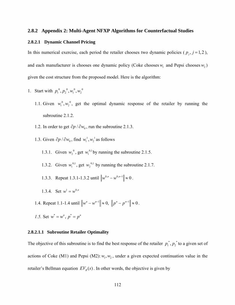
112

2.8.2 Appendix 2: Multi-Agent NFXP Algorithms for Counterfactual Studies

2.8.2.1 Dynamic Channel Pricing

In this numerical exercise, each period the retailer chooses two dynamic policies ( , 1,2jp j ),

and each manufacturer is chooses one dynamic policy (Coke chooses 1w and Pepsi chooses 2w )

given the cost structure from the proposed model. Here is the algorithm:

1. Start with 0 0 0 01 2 1 2, , ,p p w w

1.1. Given 0 01 2,w w , get the optimal dynamic response of the retailer by running the

subroutine 2.1.2.

1.2. In order to get 0/p w , run the subroutine 2.1.3.

1.3. Given 0/p w , find 1 11 2,w w as follows

1.3.1. Given 02w , get 0,1

1w by running the subroutine 2.1.5.

1.3.2. Given 0,11w , get 0,1


1.3.3. Repeat 1.3.1-1.3.2 until 0, 0, 1 0n nw w .

1.3.4. Set 1 0,nw w

1.4. Repeat 1.1-1.4 until 1 10, 0n n n nw w p p .

1.5. Set * *, n nw w p p

2.8.2.1.1 Subroutine Retailer Optimality

The objective of this subroutine is to find the best response of the retailer * *1 2,p p to a given set of

actions of Coke (M1) and Pepsi (M2): 1 2,w w , under a given expected continuation value in the

retailer’s Bellman equation ( )REV s . In other words, the objective is given by

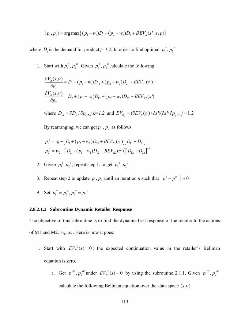
113

1 2 1 1 1 2 2 2( , ) arg max ( ) ( ) ( ' | , )Rp p p w D p w D EV s s p

where jD is the demand for product j=1,2. In order to find optimal * *1 2,p p

1. Start with 0 01 2,p p . Given 0 0

1 2,p p calculate the following:

1 1 1 11 2 2 21 11

2 1 1 12 2 2 22 22

( , )( ) ( ) ( ')

( , )( ) ( ) ( ')

RR

RR

V sD p w D p w D BEV s

p

V sD p w D p w D BEV s

p

where /jk j kD D p , j,k=1,2, and ( ( ') / ')( '/ ), 1,2R j R jEV EV s s s p j

By rearranging, we can get 1 11 2,p p as follows:

111 1 1 2 2 21 1 11 21

112 2 2 1 1 12 2 12 22

( ) ( ')

( ) ( ')

R

R

p w D p w D BEV s D D

p w D p w D BEV s D D

2. Given 1 11 2,p p , repeat step 1, to get 2 2

1 2,p p

3. Repeat step 2 to update 1 2,p p until an iteration n such that 1 0n np p

4. Set * *1 1 2 2,n np p p p

2.8.2.1.2 Subroutine Dynamic Retailer Response

The objective of this subroutine is to find the dynamic best response of the retailer to the actions

of M1 and M2: 1 2,w w . Here is how it goes:

1. Start with 0 ( ) 0REV s : the expected continuation value in the retailer’s Bellman

equation is zero.

a. Get 0* 0*1 2,p p under 0 ( ) 0REV s by using the subroutine 2.1.1. Given 0* 0*

1 2,p p

calculate the following Bellman equation over the state space ( , )s

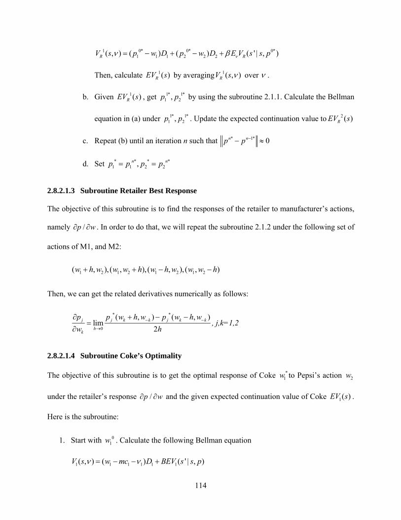
114

1 0* 0* 0*1 1 1 2 2 2( , ) ( ) ( ) ( ' | , )R RV s p w D p w D E V s s p

Then, calculate 1( )REV s by averaging 1( , )RV s over .

b. Given 1( )REV s , get 1* 1*1 2,p p by using the subroutine 2.1.1. Calculate the Bellman

equation in (a) under 1* 1*1 2,p p . Update the expected continuation value to 2 ( )REV s

c. Repeat (b) until an iteration n such that * 1* 0n np p

d. Set * * * *1 1 2 2,n np p p p

2.8.2.1.3 Subroutine Retailer Best Response

The objective of this subroutine is to find the responses of the retailer to manufacturer’s actions,

namely /p w . In order to do that, we will repeat the subroutine 2.1.2 under the following set of

actions of M1, and M2:

1 2 1 2 1 2 1 2( , ), ( , ), ( , ), ( , )w h w w w h w h w w w h

Then, we can get the related derivatives numerically as follows:

* *

0

( , ) ( , )lim

2j j k k j k k

hk

p p w h w p w h w

w h

, j,k=1,2

2.8.2.1.4 Subroutine Coke’s Optimality

The objective of this subroutine is to get the optimal response of Coke *1w to Pepsi’s action 2w

under the retailer’s response /p w and the given expected continuation value of Coke 1( )EV s .

Here is the subroutine:

1. Start with 01w . Calculate the following Bellman equation

1 1 1 1 1 1( , ) ( ) ( ' | , )V s w mc D BEV s s p

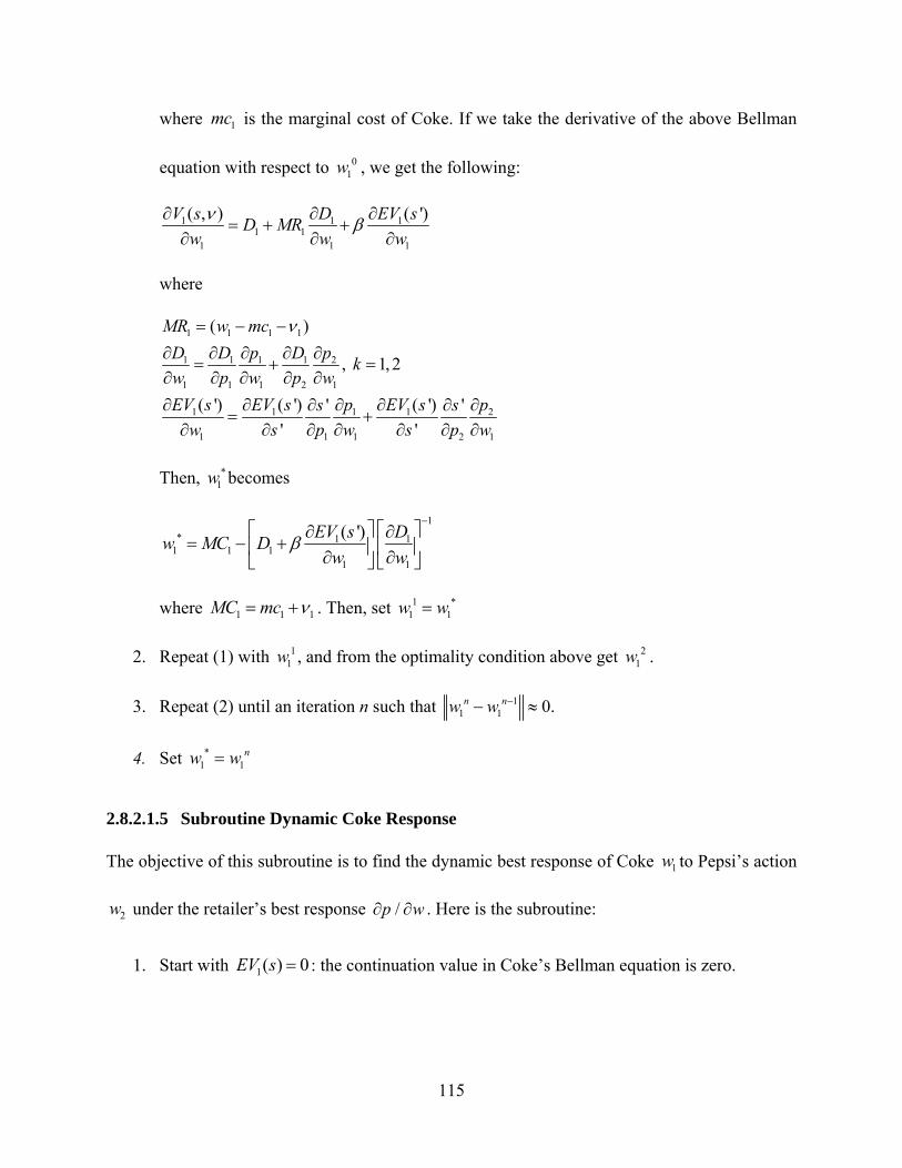
115

where 1mc is the marginal cost of Coke. If we take the derivative of the above Bellman

equation with respect to 01w , we get the following:

1 1 11 1

1 1 1

( , ) ( ')V s D EV sD MR

w w w

where

1 1 1 1

1 1 1 1 2

1 1 1 2 1

1 1 1 1 2

1 1 1 2 1

( )

, 1, 2

( ') ( ') ( ')' '

' '

MR w mc

D D p D pk

w p w p w

EV s EV s p EV s ps s

w s p w s p w

Then, *1w becomes

1

* 1 11 1 1

1 1

( ')EV s Dw MC D

w w

where 1 1 1MC mc . Then, set 1 *

1 1w w

2. Repeat (1) with 11w , and from the optimality condition above get 2

1w .

3. Repeat (2) until an iteration n such that 11 1 0.n nw w

4. Set *1 1

nw w

2.8.2.1.5 Subroutine Dynamic Coke Response

The objective of this subroutine is to find the dynamic best response of Coke 1w to Pepsi’s action

2w under the retailer’s best response /p w . Here is the subroutine:

1. Start with 1( ) 0EV s : the continuation value in Coke’s Bellman equation is zero.

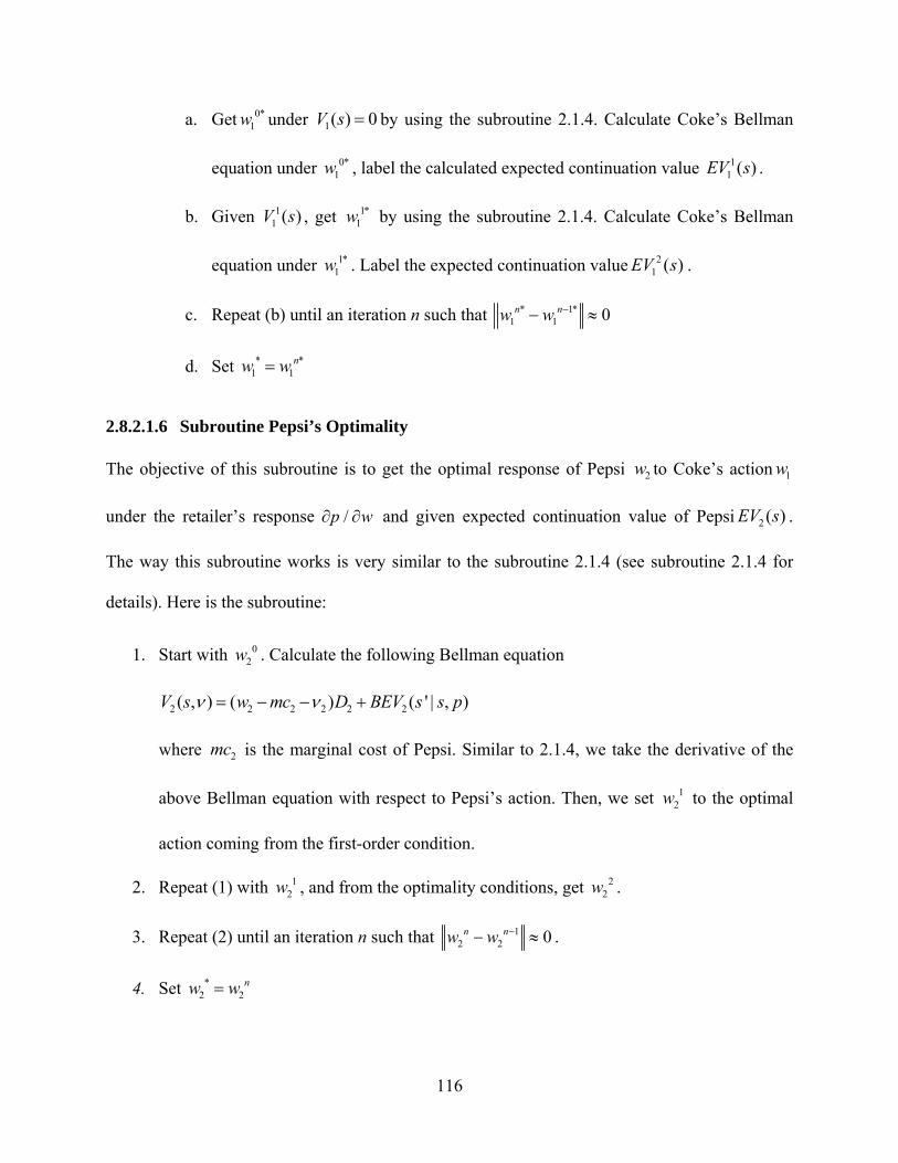
116

a. Get 0*1w under 1( ) 0V s by using the subroutine 2.1.4. Calculate Coke’s Bellman

equation under 0*1w , label the calculated expected continuation value 1

1 ( )EV s .

b. Given 11 ( )V s , get 1*

1w by using the subroutine 2.1.4. Calculate Coke’s Bellman

equation under 1*1w . Label the expected continuation value 2

1 ( )EV s .

c. Repeat (b) until an iteration n such that * 1*1 1 0n nw w

d. Set * *1 1

nw w

2.8.2.1.6 Subroutine Pepsi’s Optimality

The objective of this subroutine is to get the optimal response of Pepsi 2w to Coke’s action 1w

under the retailer’s response /p w and given expected continuation value of Pepsi 2 ( )EV s .

The way this subroutine works is very similar to the subroutine 2.1.4 (see subroutine 2.1.4 for

details). Here is the subroutine:


2 2 2 2 2 2( , ) ( ) ( ' | , )V s w mc D BEV s s p

where 2mc is the marginal cost of Pepsi. Similar to 2.1.4, we take the derivative of the

above Bellman equation with respect to Pepsi’s action. Then, we set 12w to the optimal

action coming from the first-order condition.

2. Repeat (1) with 12w , and from the optimality conditions, get 2

2w .

3. Repeat (2) until an iteration n such that 12 2 0n nw w .

4. Set *2 2

nw w

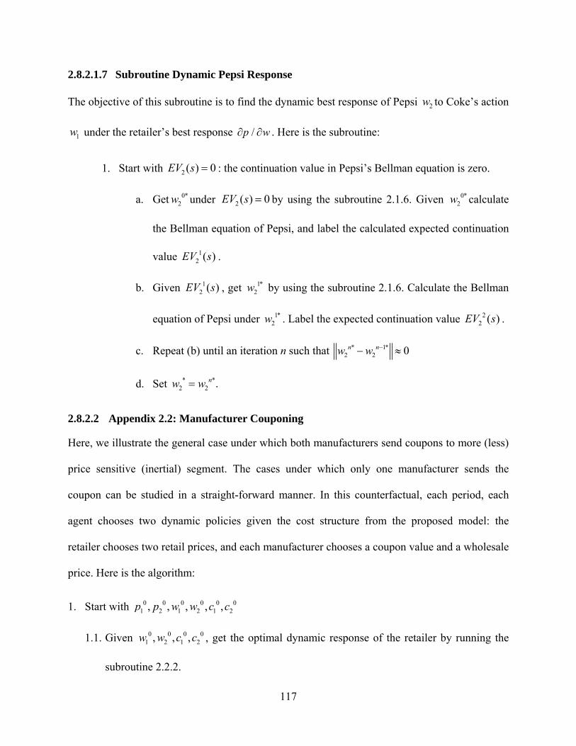
117

2.8.2.1.7 Subroutine Dynamic Pepsi Response

The objective of this subroutine is to find the dynamic best response of Pepsi 2w to Coke’s action


1. Start with 2 ( ) 0EV s : the continuation value in Pepsi’s Bellman equation is zero.

a. Get 0*2w under 2 ( ) 0EV s by using the subroutine 2.1.6. Given 0*

2w calculate

the Bellman equation of Pepsi, and label the calculated expected continuation

value 12 ( )EV s .

b. Given 12 ( )EV s , get 1*

2w by using the subroutine 2.1.6. Calculate the Bellman

equation of Pepsi under 1*2w . Label the expected continuation value 2

2 ( )EV s .


d. Set * *2 2 .nw w

2.8.2.2 Appendix 2.2: Manufacturer Couponing

Here, we illustrate the general case under which both manufacturers send coupons to more (less)

price sensitive (inertial) segment. The cases under which only one manufacturer sends the

coupon can be studied in a straight-forward manner. In this counterfactual, each period, each

agent chooses two dynamic policies given the cost structure from the proposed model: the

retailer chooses two retail prices, and each manufacturer chooses a coupon value and a wholesale

price. Here is the algorithm:

1. Start with 0 0 0 0 0 01 2 1 2 1 2, , , , ,p p w w c c

1.1. Given 0 0 0 01 2 1 2, , ,w w c c , get the optimal dynamic response of the retailer by running the

subroutine 2.2.2.

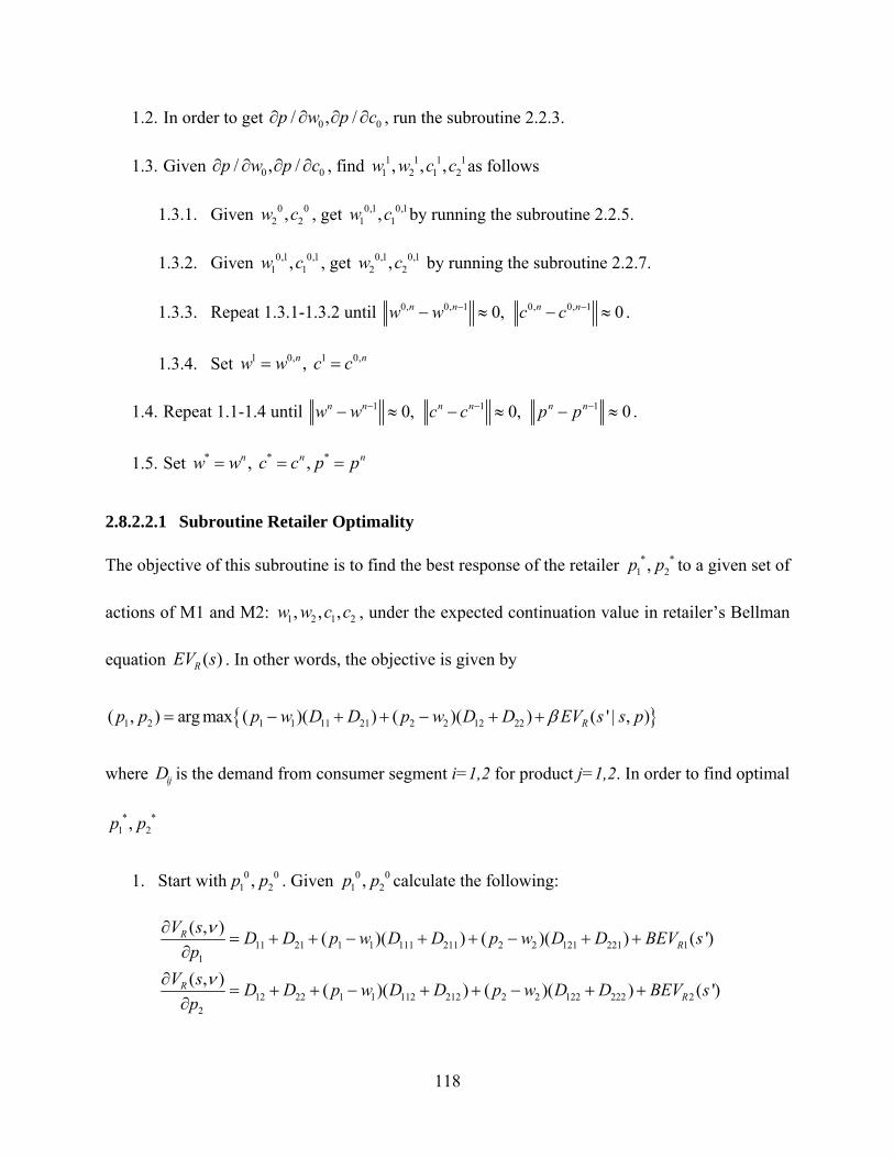
118

1.2. In order to get 0 0/ , /p w p c , run the subroutine 2.2.3.

1.3. Given 0 0/ , /p w p c , find 1 1 1 11 2 1 2, , ,w w c c as follows

1.3.1. Given 0 02 2,w c , get 0,1 0,1

1 1,w c by running the subroutine 2.2.5.

1.3.2. Given 0,1 0,11 1,w c , get 0,1 0,1

2 2,w c by running the subroutine 2.2.7.

1.3.3. Repeat 1.3.1-1.3.2 until 0, 0, 1 0, 0, 10, 0n n n nw w c c .

1.3.4. Set 1 0, 1 0,, n nw w c c

1.4. Repeat 1.1-1.4 until 1 1 10, 0, 0n n n n n nw w c c p p .

1.5. Set * * *, , n n nw w c c p p


The objective of this subroutine is to find the best response of the retailer * *1 2,p p to a given set of

actions of M1 and M2: 1 2 1 2, , ,w w c c , under the expected continuation value in retailer’s Bellman

equation ( )REV s . In other words, the objective is given by

1 2 1 1 11 21 2 2 12 22( , ) arg max ( )( ) ( )( ) ( ' | , )Rp p p w D D p w D D EV s s p

where ijD is the demand from consumer segment i=1,2 for product j=1,2. In order to find optimal

* *1 2,p p

1. Start with 0 01 2,p p . Given 0 0

1 2,p p calculate the following:

11 21 1 1 111 211 2 2 121 221 11

12 22 1 1 112 212 2 2 122 222 22

( , )( )( ) ( )( ) ( ')

( , )( )( ) ( )( ) ( ')

RR

RR

V sD D p w D D p w D D BEV s

p

V sD D p w D D p w D D BEV s

p

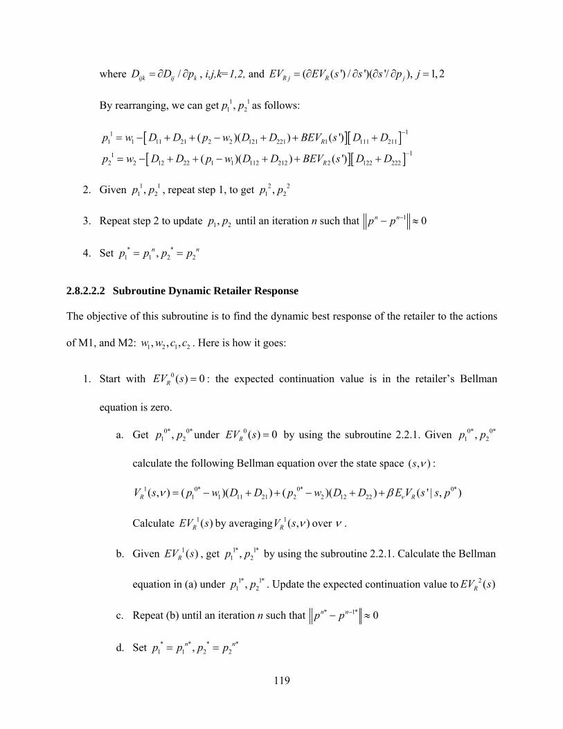
119

where /ijk ij kD D p , i,j,k=1,2, and ( ( ') / ')( '/ ), 1,2R j R jEV EV s s s p j

By rearranging, we can get 1 11 2,p p as follows:

111 1 11 21 2 2 121 221 1 111 211

112 2 12 22 1 1 112 212 2 122 222

( )( ) ( ')

( )( ) ( ')

R

R

p w D D p w D D BEV s D D

p w D D p w D D BEV s D D

2. Given 1 11 2,p p , repeat step 1, to get 2 2

1 2,p p

3. Repeat step 2 to update 1 2,p p until an iteration n such that 1 0n np p

4. Set * *1 1 2 2,n np p p p



of M1, and M2: 1 2 1 2, , ,w w c c . Here is how it goes:

1. Start with 0 ( ) 0REV s : the expected continuation value is in the retailer’s Bellman

equation is zero.

a. Get 0* 0*1 2,p p under 0 ( ) 0REV s by using the subroutine 2.2.1. Given 0* 0*

1 2,p p

calculate the following Bellman equation over the state space ( , )s :

1 0* 0* 0*1 1 11 21 2 2 12 22( , ) ( )( ) ( )( ) ( ' | , )R RV s p w D D p w D D E V s s p

Calculate 1( )REV s by averaging 1( , )RV s over .

b. Given 1( )REV s , get 1* 1*1 2,p p by using the subroutine 2.2.1. Calculate the Bellman

equation in (a) under 1* 1*1 2,p p . Update the expected continuation value to 2 ( )REV s


d. Set * * * *1 1 2 2,n np p p p

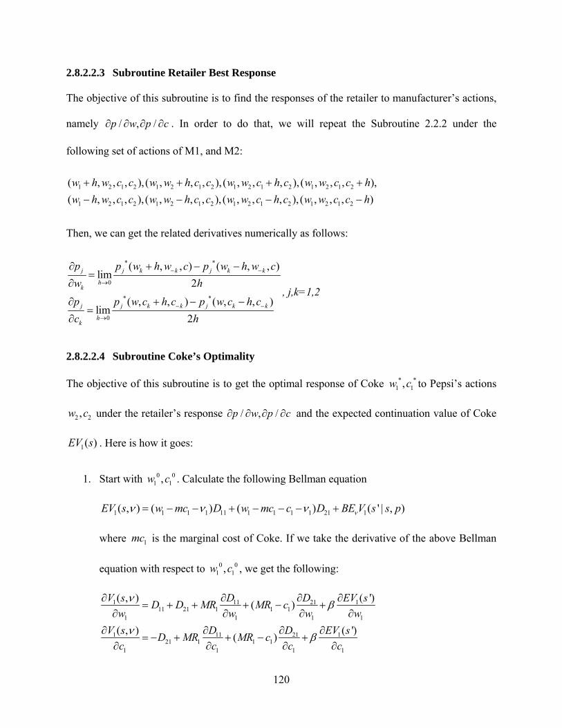
120



namely / , /p w p c . In order to do that, we will repeat the Subroutine 2.2.2 under the

following set of actions of M1, and M2:

1 2 1 2 1 2 1 2 1 2 1 2 1 2 1 2

1 2 1 2 1 2 1 2 1 2 1 2 1 2 1 2

( , , , ), ( , , , ), ( , , , ), ( , , , ),

( , , , ), ( , , , ), ( , , , ), ( , , , )

w h w c c w w h c c w w c h c w w c c h

w h w c c w w h c c w w c h c w w c c h


* *

0

* *

0

( , , ) ( , , )lim

2

( , , ) ( , , )lim

2

j j k k j k k

hk

j j k k j k k

hk

p p w h w c p w h w c

w h

p p w c h c p w c h c

c h

, j,k=1,2


The objective of this subroutine is to get the optimal response of Coke * *1 1,w c to Pepsi’s actions

2 2,w c under the retailer’s response / , /p w p c and the expected continuation value of Coke

1( )EV s . Here is how it goes:

1. Start with 0 01 1,w c . Calculate the following Bellman equation

1 1 1 1 11 1 1 1 1 21 1( , ) ( ) ( ) ( ' | , )EV s w mc D w mc c D BE V s s p


equation with respect to 0 01 1,w c , we get the following:

1 11 21 111 21 1 1 1

1 1 1 1

1 11 21 121 1 1 1

1 1 1 1

( , ) ( ')( )

( , ) ( ')( )

V s D D EV sD D MR MR c

w w w w

V s D D EV sD MR MR c

c c c c

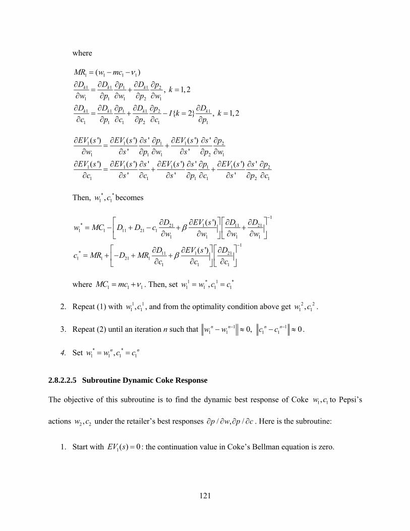
121

where

1 1 1 1

1 1 11 2

1 1 1 2 1

1 1 1 11 2

1 1 1 2 1 1

( )

, 1, 2

{ 2} , 1, 2

k k k

k k k k

MR w mc

D D Dp pk

w p w p w

D D D Dp pI k k

c p c p c p

1 1 1 1 2

1 1 1 2 1

1 1 1 1 1 2

1 1 1 1 2 1

( ') ( ') ( ')' '

' '

( ') ( ') ( ') ( ')' ' '

' ' '

EV s EV s p EV s ps s

w s p w s p w

EV s EV s EV s p EV s ps s s

c s c s p c s p c

Then, * *1 1,w c becomes

1

* 21 1 11 211 1 11 21 1

1 1 1 1

1

* 11 1 211 1 21 1

1 1 1

( ')

( ')

D EV s D Dw MC D D c

w w w w

D EV s Dc MR D MR

c c c

where 1 1 1MC mc . Then, set 1 * 1 *1 1 1 1,w w c c

2. Repeat (1) with 1 11 1,w c , and from the optimality condition above get 2 2

1 1,w c .

3. Repeat (2) until an iteration n such that 1 11 1 1 10, 0n n n nw w c c .

4. Set * *1 1 1 1,n nw w c c


The objective of this subroutine is to find the dynamic best response of Coke 1 1,w c to Pepsi’s

actions 2 2,w c under the retailer’s best responses / , /p w p c . Here is the subroutine:

1. Start with 1( ) 0EV s : the continuation value in Coke’s Bellman equation is zero.

122

a. Get 0* 0*1 1,w c under 1( ) 0EV s by using the subroutine 2.2.4. Calculate Coke’s

Bellman equation under 0* 0*1 1,w c , label the calculated Bellman equation 1

1 ( )EV s .

b. Given 11 ( )EV s , get 1* 1*

1 1,w c by using the subroutine 2.2.4. Calculate Coke’s

Bellman equation under 1* 1*1 1,w c . Label the expected continuation value 2

1 ( )EV s .

c. Repeat (b) until an iteration n such that * 1* * 1*1 1 1 10, 0n n n nw w c c

d. Set * * * *1 1 1 1,n nw w c c


The objective of this subroutine is to get the optimal response of Pepsi 2 2,w c to Coke’s actions

1 1,w c under the retailer’s response / , /p w p c and the expected continuation value of Pepsi

2 ( )EV s . Since the way this subroutine works is very similar to the subroutine 2.2.4 (see

subroutine 2.2.4 for details). Here is the subroutine:

1. Start with 0 02 2,w c . Calculate the following Bellman equation

2 2 2 2 12 2 2 2 2 22 2( , ) ( ) ( ) ( ' | , )V s w mc D w mc c D BEV s s p

where 2mc is the marginal cost of Pepsi. Similar to the subroutine 2.2.4, we take the

derivative of the above Bellman equation with respect to Pepsi’s actions. Then, we set

1 12 2,w c to the actions coming from the first-order conditions.

2. Repeat (1) with 1 12 2,w c , and from the optimality conditions, get 2 2

2 2,w c .

3. Repeat (2) until an iteration n such that 1 12 2 2 20, 0n n n nw w c c .

4. Set * *2 2 2 2,n nw w c c

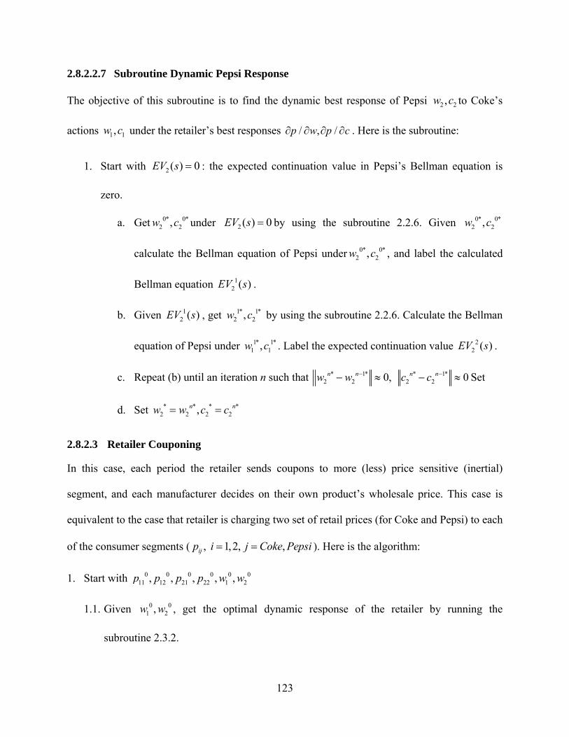
123


The objective of this subroutine is to find the dynamic best response of Pepsi 2 2,w c to Coke’s

actions 1 1,w c under the retailer’s best responses / , /p w p c . Here is the subroutine:

1. Start with 2 ( ) 0EV s : the expected continuation value in Pepsi’s Bellman equation is

zero.

a. Get 0* 0*2 2,w c under 2 ( ) 0EV s by using the subroutine 2.2.6. Given 0* 0*

2 2,w c

calculate the Bellman equation of Pepsi under 0* 0*2 2,w c , and label the calculated

Bellman equation 12 ( )EV s .

b. Given 12 ( )EV s , get 1* 1*

2 2,w c by using the subroutine 2.2.6. Calculate the Bellman

equation of Pepsi under 1* 1*1 1,w c . Label the expected continuation value 2

2 ( )EV s .

c. Repeat (b) until an iteration n such that * 1* * 1*2 2 2 20, 0n n n nw w c c Set

d. Set * * * *2 2 2 2,n nw w c c

2.8.2.3 Retailer Couponing

In this case, each period the retailer sends coupons to more (less) price sensitive (inertial)

segment, and each manufacturer decides on their own product’s wholesale price. This case is

equivalent to the case that retailer is charging two set of retail prices (for Coke and Pepsi) to each

of the consumer segments ( , 1,2, ,ijp i j Coke Pepsi ). Here is the algorithm:

1. Start with 0 0 0 0 0 011 12 21 22 1 2, , , , ,p p p p w w

1.1. Given 0 01 2,w w , get the optimal dynamic response of the retailer by running the

subroutine 2.3.2.

124

1.2. In order to get 0/p w , run the subroutine 2.3.3.

1.3. Given 0/p w , find 1 11 2,w w as follows

1.3.1. Given 02w , get 0,1


1.3.2. Given 0,11w , get 0,1


1.3.3. Repeat 1.3.1-1.3.2 until 0, 0, 1 0n nw w .

1.3.4. Set 1 0,nw w

1.4. Repeat 1.1-1.4 until 1 10, 0n n n nw w p p .

1.5. Set * *, n nw w p p


The objective of this subroutine is to find the best response of the retailer * * * *11 12 21 22, , ,p p p p to a

given set of actions of M1 and M2: 1 2,w w , under the expected continuation value in retailer’s

Bellman equation ( )REV s . In other words, the objective is given by

11 1 11 21 1 21 12 2 12 12 2 2211 12 21 22

( ) ( ) ( ) ( )( , , , ) arg max

( ' | , )R

p w D p w D p w D p w Dp p p p

EV s s p

where ijD is the demand from consumer segment i=1,2 for product j=1,2. In order to find optimal

* * * *11 12 21 22, , ,p p p p

1. Start with 0 0 0 011 12 21 22, , ,p p p p . Given 0 0 0 0

11 12 21 22, , ,p p p p calculate the following:

11 1 111 12 2 121 11

11 1 112 12 2 122 12

21 1 211 22

1

2 221 21

1 11

12 1

21

2

21 21

2 2 12 2

) ( ) ( ' | , )

) ( ) ( ' | ,

( , ) / (

( , ) / (

( , )

)

( ) ( ) ( ' | , )

(

/

( , )) /

RR

R

R

R

R

R

V s p D

V s

p w D p w D EV s s p



p D

V s p D

V s p D p w

212 22 2 222 22( ) ( ' | , )RD p w D EV s s p

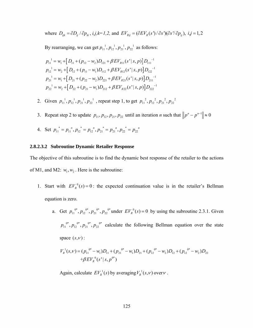
125

where /ijk ij ikD D p , i,j,k=1,2, and ( ( ') / ')( '/ ), , 1,2Rij R ijEV EV s s s p i j

By rearranging, we can get 1 1 1 111 12 21 22, , ,p p p p as follows:

111 11

112 2 1

11 12 2 121 11 111

111 1 112

121 1 21

122

2 12 122

122 2 221 21 211

121 1 212 22 222 2 22

( ) ( ' | , )

) ( ' | , )

( ) ( ' | , )

( ) ( ' | , )

(

R

R

R

R

p D

p w D

p

w p w D EV s s p D

p w D EV s s p D

p w D EV s s p D

p w D EV

w D

p sw D s p D

2. Given 1 1 1 111 12 21 22, , ,p p p p , repeat step 1, to get 2 2 2 2

11 12 21 22, , ,p p p p

3. Repeat step 2 to update 11 12 21 22, , ,p p p p until an iteration n such that 1 0n np p

4. Set * * * *11 11 12 12 21 21 22 22, , ,n n n np p p p p p p p



of M1, and M2: 1 2,w w . Here is the subroutine:

1. Start with 0 ( ) 0REV s : the expected continuation value is in the retailer’s Bellman

equation is zero.

a. Get 0* 0* 0* 0*11 12 21 22, , ,p p p p under 0 ( ) 0REV s by using the subroutine 2.3.1. Given

0* 0* 0* 0*11 12 21 22, , ,p p p p calculate the following Bellman equation over the state

space ( , )s :

1 0* 0* 0* 0*11 1 11 21 1 21 12 2 12 12 2 22

0 0*

( , ) ( ) ( ) ( ) ( )

+ ( ' | , )

R

R

V s p w D p w D p w D p w D

EV s s p

Again, calculate 1( )REV s by averaging 1( , )RV s over .

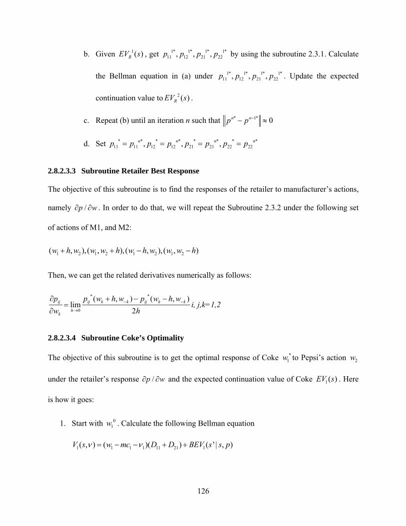
126

b. Given 1( )REV s , get 1* 1* 1* 1*11 12 21 22, , ,p p p p by using the subroutine 2.3.1. Calculate

the Bellman equation in (a) under 1* 1* 1* 1*11 12 21 22, , ,p p p p . Update the expected

continuation value to 2 ( )REV s .


d. Set * * * * * * * *11 11 12 12 21 21 22 22, , ,n n n np p p p p p p p



namely /p w . In order to do that, we will repeat the Subroutine 2.3.2 under the following set

of actions of M1, and M2:

1 2 1 2 1 2 1 2( , ), ( , ), ( , ), ( , )w h w w w h w h w w w h


* *

0

( , ) ( , )lim

2ij ij k k ij k k

hk

p p w h w p w h w

w h

i, j,k=1,2


The objective of this subroutine is to get the optimal response of Coke *1w to Pepsi’s action 2w

under the retailer’s response /p w and the expected continuation value of Coke 1( )EV s . Here

is how it goes:


1 1 1 1 11 21 1( , ) ( )( ) ( ' | , )V s w mc D D BEV s s p

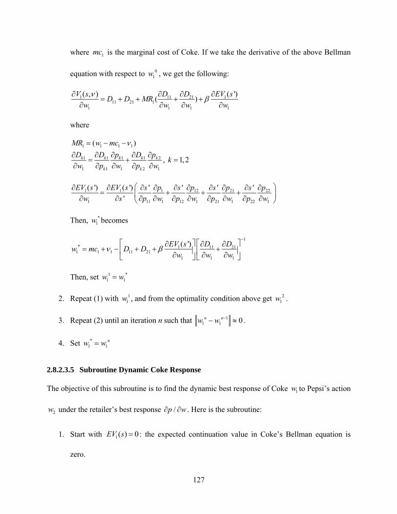
127


equation with respect to 01w , we get the following:

1 11 21 111 21 1

1 1 1 1

( , ) ( ')( )

V s D D EV sD D MR

w w w w

where

1 1 1 1

1 1 1 1 2

1 1 1 2 1

( )

, 1, 2k k k k k

k k

MR w mc

D D p D pk

w p w p w

1 1 1 12 21 22

1 11 1 12 1 21 1 22 1

( ') ( ') ' ' ' '

'

EV s EV s p p p ps s s s

w s p w p w p w p w

Then, *1w becomes

1

* 1 11 211 1 1 11 21

1 1 1

( ')EV s D Dw mc D D

w w w

Then, set 1 *

1 1w w

2. Repeat (1) with 11w , and from the optimality condition above get 2

1w .


4. Set *1 1

nw w


The objective of this subroutine is to find the dynamic best response of Coke 1w to Pepsi’s action


1. Start with 1( ) 0EV s : the expected continuation value in Coke’s Bellman equation is

zero.

128

a. Get 0*1w under 1( ) 0EV s by using the subroutine 2.3.4. Calculate Coke’s Bellman

equation under 0*1w , label the calculated Bellman equation 1

1 ( )EV s .


1w by using the subroutine 2.3.4. Calculate Coke’s Bellman

equation under 1*1w . Label the expected continuation value 2

1 ( )EV s .


d. Set * *1 1

nw w


The objective of this subroutine is to get the optimal response of Pepsi 2w to Coke’s action 1w

under the retailer’s response /p w and the expected continuation value of Pepsi 2 ( )V s . Since

the way this subroutine works is very similar to the subroutine 2.3.4 (see subroutine 2.3.4 for

details). Here is the subroutine:


2 2 2 2 12 22 2( , ) ( )( ) ( ' | , )V s w mc D D BEV s s p

where 2mc is the marginal cost of Pepsi. Similar to the subroutine 2.3.4, we take the

derivative of the above Bellman equation with respect to Pepsi’s actions. Then, we set

12w to the actions coming from the first-order conditions.

2. Repeat (1) with 12w , and from the optimality conditions, get 2

2w .


4. Set *2 2

nw w

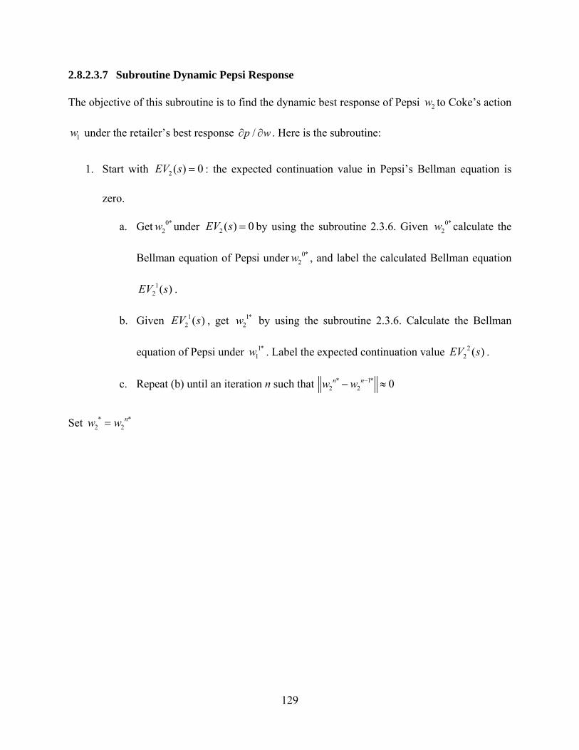
129


The objective of this subroutine is to find the dynamic best response of Pepsi 2w to Coke’s action


1. Start with 2 ( ) 0EV s : the expected continuation value in Pepsi’s Bellman equation is

zero.

a. Get 0*2w under 2 ( ) 0EV s by using the subroutine 2.3.6. Given 0*

2w calculate the

Bellman equation of Pepsi under 0*2w , and label the calculated Bellman equation

12 ( )EV s .


2w by using the subroutine 2.3.6. Calculate the Bellman

equation of Pepsi under 1*1w . Label the expected continuation value 2

2 ( )EV s .


Set * *2 2

nw w

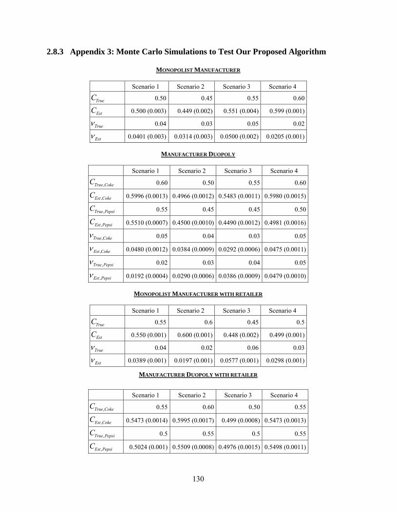
130

2.8.3 Appendix 3: Monte Carlo Simulations to Test Our Proposed Algorithm

MONOPOLIST MANUFACTURER

Scenario 1 Scenario 2 Scenario 3 Scenario 4

TrueC 0.50 0.45 0.55 0.60

EstC 0.500 (0.003) 0.449 (0.002) 0.551 (0.004) 0.599 (0.001)

True 0.04 0.03 0.05 0.02

Est 0.0401 (0.003) 0.0314 (0.003) 0.0500 (0.002) 0.0205 (0.001)

MANUFACTURER DUOPOLY


,True CokeC 0.60 0.50 0.55 0.60

,Est CokeC 0.5996 (0.0013) 0.4966 (0.0012) 0.5483 (0.0011) 0.5980 (0.0015)

,True PepsiC 0.55 0.45 0.45 0.50

,Est PepsiC 0.5510 (0.0007) 0.4500 (0.0010) 0.4490 (0.0012) 0.4981 (0.0016)

,True Coke 0.05 0.04 0.03 0.05

,Est Coke 0.0480 (0.0012) 0.0384 (0.0009) 0.0292 (0.0006) 0.0475 (0.0011)

,True Pepsi 0.02 0.03 0.04 0.05

,Est Pepsi 0.0192 (0.0004) 0.0290 (0.0006) 0.0386 (0.0009) 0.0479 (0.0010)

MONOPOLIST MANUFACTURER WITH RETAILER


TrueC 0.55 0.6 0.45 0.5

EstC 0.550 (0.001) 0.600 (0.001) 0.448 (0.002) 0.499 (0.001)

True 0.04 0.02 0.06 0.03

Est 0.0389 (0.001) 0.0197 (0.001) 0.0577 (0.001) 0.0298 (0.001)

MANUFACTURER DUOPOLY WITH RETAILER


,True CokeC 0.55 0.60 0.50 0.55

,Est CokeC 0.5473 (0.0014) 0.5995 (0.0017) 0.499 (0.0008) 0.5473 (0.0013)

,True PepsiC 0.5 0.55 0.5 0.55

,Est PepsiC 0.5024 (0.001) 0.5509 (0.0008) 0.4976 (0.0015) 0.5498 (0.0011)

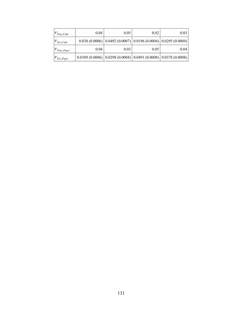
131

,True Coke 0.04 0.05 0.02 0.03

,Est Coke 0.038 (0.0006) 0.0492 (0.0007) 0.0196 (0.0004) 0.0295 (0.0004)

,True Pepsi 0.04 0.03 0.05 0.04

,Est Pepsi 0.0389 (0.0006) 0.0298 (0.0004) 0.0491 (0.0008) 0.0378 (0.0008)

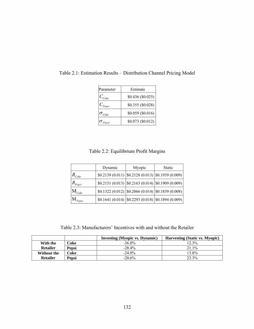
132

Table 2.1: Estimation Results – Distribution Channel Pricing Model

Parameter Estimate

CokeC $0.436 ($0.025)

PepsiC $0.355 ($0.028)

Coke $0.059 ($0.016)

Pepsi $0.073 ($0.012)

Table 2.2: Equilibrium Profit Margins

Dynamic Myopic Static

CokeR $0.2139 (0.011) $0.2128 (0.013) $0.1939 (0.009)

PepsiR $0.2151 (0.013) $0.2163 (0.014) $0.1909 (0.009)

MCoke $0.1322 (0.012) $0.2066 (0.014) $0.1839 (0.008)

MPepsi $0.1641 (0.014) $0.2293 (0.018) $0.1894 (0.009)

Table 2.3: Manufacturers’ Incentives with and without the Retailer

Investing (Myopic vs. Dynamic) Harvesting (Static vs. Myopic) With the Retailer

Coke -36.0% 12.3% Pepsi -28.4% 21.1%

Without the Retailer

Coke -24.0% 13.8% Pepsi -20.6% 23.3%

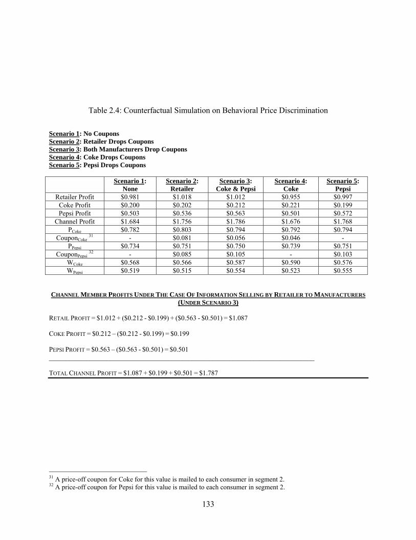
133

Table 2.4: Counterfactual Simulation on Behavioral Price Discrimination

Scenario 1: No Coupons Scenario 2: Retailer Drops Coupons Scenario 3: Both Manufacturers Drop Coupons Scenario 4: Coke Drops Coupons Scenario 5: Pepsi Drops Coupons

Scenario 1: None

Scenario 2: Retailer

Scenario 3: Coke & Pepsi

Scenario 4: Coke

Scenario 5: Pepsi

Retailer Profit $0.981 $1.018 $1.012 $0.955 $0.997 Coke Profit $0.200 $0.202 $0.212 $0.221 $0.199 Pepsi Profit $0.503 $0.536 $0.563 $0.501 $0.572

Channel Profit $1.684 $1.756 $1.786 $1.676 $1.768 PCoke $0.782 $0.803 $0.794 $0.792 $0.794

CouponCoke 31 - $0.081 $0.056 $0.046 -

PPepsi $0.734 $0.751 $0.750 $0.739 $0.751 CouponPepsi

32 - $0.085 $0.105 - $0.103 WCoke $0.568 $0.566 $0.587 $0.590 $0.576 WPepsi $0.519 $0.515 $0.554 $0.523 $0.555

CHANNEL MEMBER PROFITS UNDER THE CASE OF INFORMATION SELLING BY RETAILER TO MANUFACTURERS

(UNDER SCENARIO 3) RETAIL PROFIT = $1.012 + ($0.212 - $0.199) + ($0.563 - $0.501) = $1.087 COKE PROFIT = $0.212 – ($0.212 - $0.199) = $0.199 PEPSI PROFIT = $0.563 – ($0.563 - $0.501) = $0.501 ______________________________________________________________________________ TOTAL CHANNEL PROFIT = $1.087 + $0.199 + $0.501 = $1.787

31 A price-off coupon for Coke for this value is mailed to each consumer in segment 2. 32 A price-off coupon for Pepsi for this value is mailed to each consumer in segment 2.

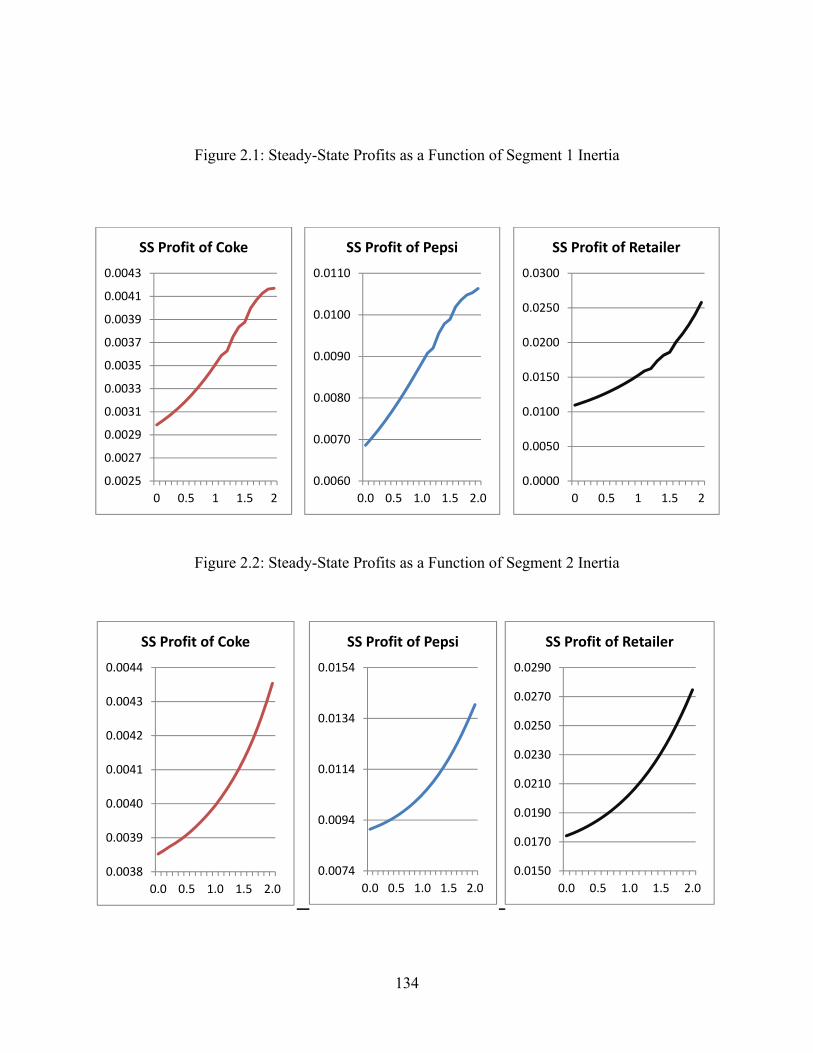
134



0.0025

0.0027

0.0029

0.0031

0.0033

0.0035

0.0037

0.0039

0.0041

0.0043

0 0.5 1 1.5 2

SS Profit of Coke

0.0060

0.0070

0.0080

0.0090

0.0100

0.0110

0.0 0.5 1.0 1.5 2.0

SS Profit of Pepsi

0.0000

0.0050

0.0100

0.0150

0.0200

0.0250

0.0300

0 0.5 1 1.5 2

SS Profit of Retailer

0.0038

0.0039

0.0040

0.0041

0.0042

0.0043

0.0044

0.0 0.5 1.0 1.5 2.0

SS Profit of Coke

0.0074

0.0094

0.0114

0.0134

0.0154

0.0 0.5 1.0 1.5 2.0

SS Profit of Pepsi

0.0150

0.0170

0.0190

0.0210

0.0230

0.0250

0.0270

0.0290

0.0 0.5 1.0 1.5 2.0

SS Profit of Retailer

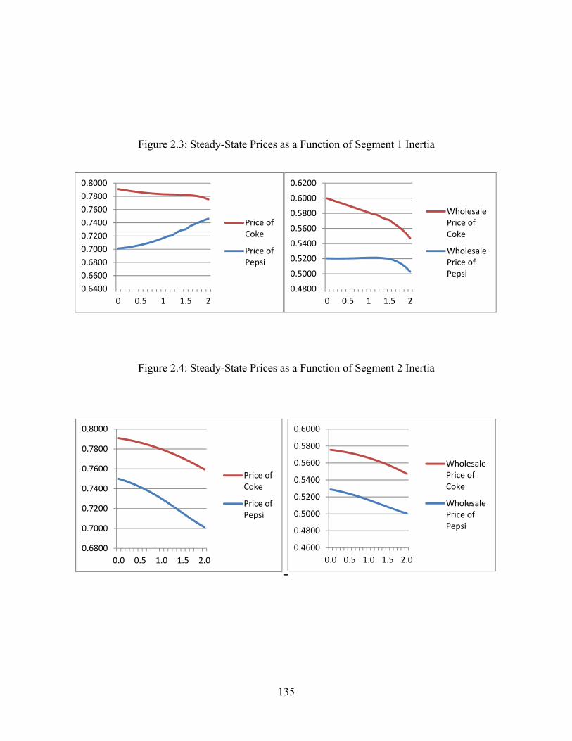
135



0.6400

0.6600

0.6800

0.7000

0.7200

0.7400

0.7600

0.7800

0.8000

0 0.5 1 1.5 2

Price ofCoke

Price ofPepsi

0.4800

0.5000

0.5200

0.5400

0.5600

0.5800

0.6000

0.6200

0 0.5 1 1.5 2

WholesalePrice ofCoke

WholesalePrice ofPepsi

0.6800

0.7000

0.7200

0.7400

0.7600

0.7800

0.8000

0.0 0.5 1.0 1.5 2.0

Price ofCoke

Price ofPepsi

0.4600

0.4800

0.5000

0.5200

0.5400

0.5600

0.5800

0.6000

0.0 0.5 1.0 1.5 2.0

WholesalePrice ofCoke

WholesalePrice ofPepsi

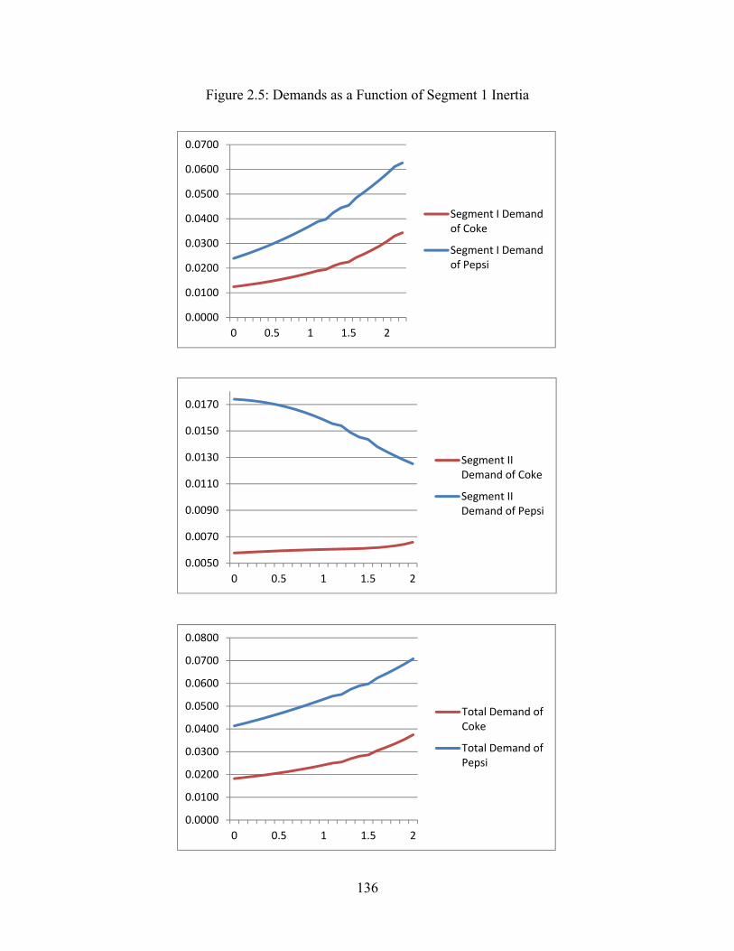
136

Figure 2.5: Demands as a Function of Segment 1 Inertia

0.0000

0.0100

0.0200

0.0300

0.0400

0.0500

0.0600

0.0700

0 0.5 1 1.5 2

Segment I Demandof Coke

Segment I Demandof Pepsi

0.0050

0.0070

0.0090

0.0110

0.0130

0.0150

0.0170

0 0.5 1 1.5 2



0.0000

0.0100

0.0200

0.0300

0.0400

0.0500

0.0600

0.0700

0.0800

0 0.5 1 1.5 2

Total Demand ofCoke

Total Demand ofPepsi

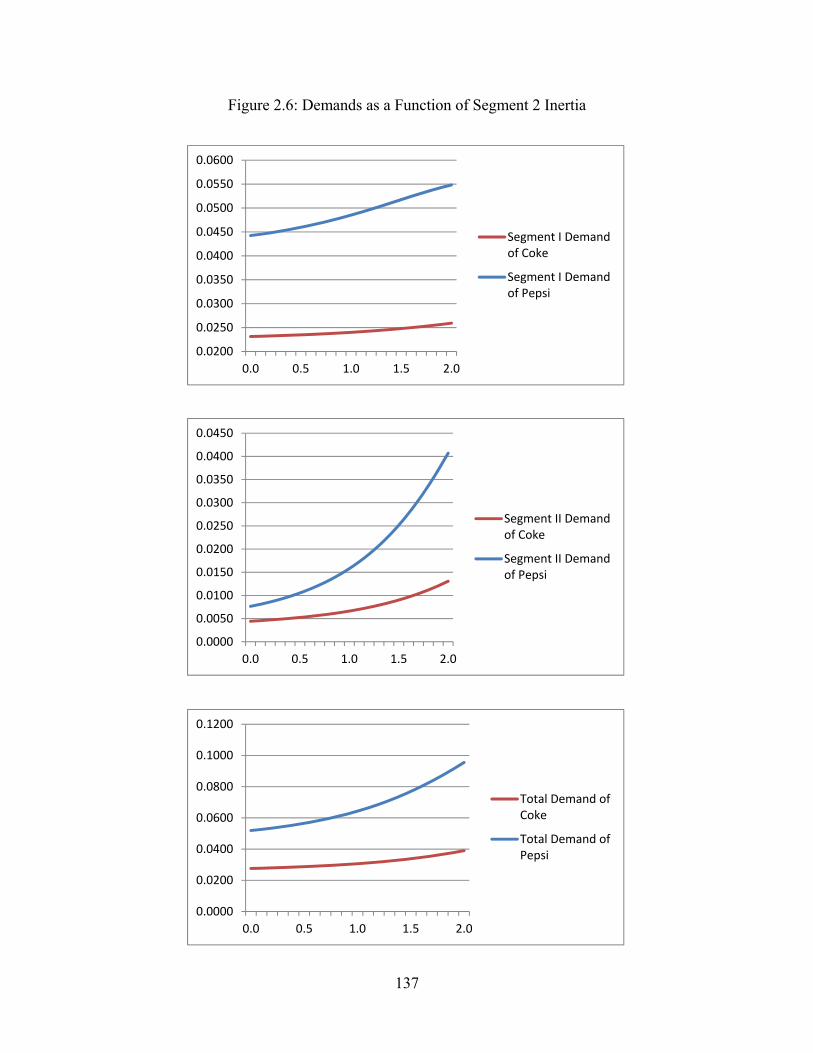
137

Figure 2.6: Demands as a Function of Segment 2 Inertia

0.0200

0.0250

0.0300

0.0350

0.0400

0.0450

0.0500

0.0550

0.0600

0.0 0.5 1.0 1.5 2.0

Segment I Demandof Coke

Segment I Demandof Pepsi

0.0000

0.0050

0.0100

0.0150

0.0200

0.0250

0.0300

0.0350

0.0400

0.0450

0.0 0.5 1.0 1.5 2.0

Segment II Demandof Coke

Segment II Demandof Pepsi

0.0000

0.0200

0.0400

0.0600

0.0800

0.1000

0.1200

0.0 0.5 1.0 1.5 2.0

Total Demand ofCoke

Total Demand ofPepsi

138

References

Ailawadi, K. L., Gedenk, K., Neslin, S. (1999). Heterogeneity and Purchase Event Feedback in

Choice Models: An Empirical Analysis with Implications for Model Building, International

Journal of Research in Marketing, 16, 3, 177-198.

Allenby, G. M., Lenk, P. J. (1995). Reassessing Brand Loyalty, Price Sensitivity and

Merchandising Effects on Consumer Brand Choice, Journal of Business and Economic

Statistics, 13, 3, 281-289.

Andrews, R. L., Ainslie, A., Currim, I. S. (2002). An Empirical Comparison of Logit Choice

Models with Discrete versus Continuous Representations of Heterogeneity, Journal of

Marketing Research, 39, 4, 479-487.

Bajari, P., Benkard, C. L., Levin, J. (2007). Estimating Dynamic Models of Imperfect

Competition, Econometrica, 75, 5, 1331-1370.

Bawa, K. (1990). Modeling Inertia and Variety Seeking Tendencies in Brand Choice Behavior,

Marketing Science, 9, 3, 87-96.

Beggs, A., Klemperer, P. (1992). Multi-Period Competition with Switching Costs, Econometrica,

57, 3, 651-666.

Berry, S., Levinsohn, J., Pakes, A. (1995). Automobile Prices in Market Equilibrium,

Econometrica, 63, 4, 841-890.

Bronnenberg, B. J., Rossi, P. E., Vilcassim, N. J. (2005). Structural Modeling and Policy

Simulation, Journal of Marketing Research, 42, 1, 22-26.

139

Che, H., Sudhir, K., Seetharaman, P. B. (2007). Bounded Rationality in Pricing Under State

Dependent Demand: Do Firms Look Ahead? How Far Ahead?, Journal of Marketing

Research, 44, 3, 434-449.

Chintagunta, P. K., Rao, V. R. (1996). Pricing Strategies in a Dynamic Duopoly: A Differential

Game Model, Management Science, 42, 11, 1501-1514.

Colombo, R. A., Morrison, D. G. (1989). A Brand Switching Model with Implications for

Marketing Strategies, Marketing Science, 8, 1, 89-99.

Draganska, M., Klapper, D., Villas-Boas, S. B. (2010). A Larger Slice or a Larger Pie? An

Empirical Investigation of Bargaining Power in the Distribution Channel, Marketing Science,

29, 1, 57-74.

Dube, J. P., Hitsch, G. J., Rossi, P. E. (2009). Do Switching Costs Make Markets Less

Competitive?, Journal of Marketing Research, 46, 3, 435-445.

Dube, J. P., Hitsch, G. J., Rossi, P. E., Vitorino, M. A. (2008). Category Pricing with State-

Dependent Utility, Marketing Science, 27, 3, 417-429.

Erdem, T. (1996). A Dynamic Analysis of Market Structure Based on Panel Data, Marketing

Science, 15, 4, 359-378.

Erdem, T., Sun, B. (2001). Testing for Choice Dynamics in Panel Data, Journal of Business and

Economic Statistics, 19, 2, 142-152.

Fader, P., Lattin, J. M. (1993). Accounting for Heterogeneity and Non-Stationarity in a Cross-

Sectional Model of Consumer Purchase Behavior, Marketing Science, 12, 3, 304-317.

140

Freimer, M., Horsky, D. (2008). Try It, You Will Like It – Does Consumer Learning Lead to

Competitive Price Promotions, Marketing Science, 27, 5, 796-810.

Givon, M., Horsky, D. (1994). Intertemporal Aggregation of Heterogeneous Consumers,

European Journal of Operational Research, 76, 2, 273-282.

Guadagni, P., Little, J. D. C. (1983). A Logit Model of Brand Choice Calibrated on Scanner

Data, Marketing Science, 2, 3, 203-238.

Gupta, S., Chintagunta, P. K., Wittink, D. R. (1997). Household Heterogeneity and State

Dependence in a Model of Purchase Strings: Empirical Results and Managerial Implications,

International Journal of Research in Marketing, 14, 4, 189-213.

Hood, W. C., Koopmans, T. C. (1953). Studies in Econometric Method, Cowles Commission

Monograph, Number 14, John Wiley, New York.

Hotz, V. J., Miller, R. A. (1993). Conditional Choice Probabilities and the Estimation of

Dynamic Models, The Review of Economic Studies, 60, 3, 497-529.

Hotz, V. J., Miller, R. A., Sanders, S., Smith, J. (1994). A Simulation Estimator for Dynamic

Models of Discrete Choice, The Review of Economic Studies, 61, 2, 265-289.

Jeuland, A. (1979). Brand Choice Inertia as One Aspect of the Notion of Brand Loyalty,

Management Science, 25, 3, 671-682.

Kadiyali, V., Chintagunta, P. K., Vilcassim, N. (2000). Power in Manufacturer-Retailer

Interactions: An Empirical Investigation of Pricing in a Local Market, Marketing Science, 19,

2, 127-148.

141

Kahn, B. E., Kalwani, M. U., Morrison, D. G. (1986). Measuring Variety Seeking and

Reinforcement Behaviors Using Panel Data, Journal of Marketing Research, 23, 2, 89-100.

Keane, M. (1997). Modeling Heterogeneity and State Dependence in Consumer Choice

Behavior, Journal of Business and Economic Statistics, 15, 3, 310-327.

Kim, M., Kliger, D., Vale, B. (2003). Estimating Switching Costs, Journal of Financial

Intermediation, 12, 1, 25-56.

Klemperer, P. (1987a). Markets with Consumer Switching Costs, The Quarterly Journal of

Economics, 102, 4, 375-394.

Klemperer, P. (1987b). The Competitiveness of Markets with Switching Costs, RAND Journal of

Economics, 18, 1, 138-150.

Moshkin, N., Shachar, R. (2002). The Asymmetric Information Model of State Dependence,

Marketing Science, 22, 4, 1-20.

Pakes, A., McGuire, P. (1994). Computing Markov-Perfect Nash Equilibria: Numerical

Implications of a Dynamic Differentiated Product Model, RAND Journal of Economics, 25,

4, 555-589.

Pakes, A., McGuire, P. (2001). Symmetric Markov-Perfect Equilibrium, Stochastic Algorithms

and the Curse of Dimensionality, Econometrica, 69, 5, 1261-1281.

Pancras, J., Sudhir, K. (2007). Optimal Marketing Strategies for a Customer Data Intermediary,

Journal of Marketing Research, 44, 4, 560-578.

142

Roy, R., Chintagunta, P. K., Haldar, S. (1996). A Framework for Investigating Habits, The Hand

of the Past, and Heterogeneity in Dynamic Brand Choice, Marketing Science, 15, 3, 280-299.

Rust, J. (1987). Optimal Replacement of GMC Bus Engines: An Empirical Model of Harold

Zurcher, Econometrica, 55, 5, 999-1033.

Sudhir, K. (2001). Structural Analysis of Manufacturer Pricing in the Presence of a Strategic

Retailer, Marketing Science, 20, 3, 244-264.

Seetharaman, P. B. (2003). Probabilistic versus Random Utility Models of State Dependence: An

Empirical Comparison, International Journal of Research in Marketing, 20, 1, 87-96.

Seetharaman, P. B. (2004). Modeling Multiple Sources of State Dependence in Random Utility

Models: A Distributed Lag Approach, Marketing Science, 23, 2, 263-271.

Seetharaman, P. B. (2009). Dynamic Pricing, in Handbook of Pricing Research in Marketing, ed.

Vithala R. Rao, Edward Elgar Publishers.

Seetharaman, P. B., Ainslie, A., Chintagunta, P. K. (1999). Investigating Household State

Dependence Effects Across Categories, Journal of Marketing Research, 36, 4, 488-500.

Seetharaman, P. B., Che, H. (2009). Price Competition in Markets with Consumer Variety

Seeking, Marketing Science, 28, 3, 516-525.

Seetharaman, P. B., Chintagunta, P. K. (1998). A Model of Inertia and Variety Seeking with

Marketing Variables, International Journal of Research in Marketing, 15, 1, 1-17.

Shum, M. (2004). Does Advertising Overcome Brand Loyalty? Evidence from the Breakfast-

Cereals Market, Journal of Economics & Management Strategy, 13, 2, 241-272.

143

Su, C. L., Judd, K. L. (2011). Constrained Optimization Approaches to Estimation of Structural

Models, Econometrica, forthcoming.

Viard, V. B. (2007). Do Switching Costs Make Markets More or Less Competitive? The Case of

800-Number Portability, The RAND Journal of Economics, 38, 1, 146-163.

Villas-Boas, J. M. (2004). Consumer Learning, Brand Loyalty, and Competition, Marketing

Science, 23, 1, 134-145.

Villas-Boas, J. M., Zhao, Y. (2005). Retailers, Manufacturers, and Individual Consumers:

Modeling the Supply Side in the Ketchup Marketplace, Journal of Marketing Research, 42, 1,

83-95.

Villas-Boas, S. B. (2007). Vertical Relationships between Manufacturers and Retailers: Inference

with Limited Data, The Review of Economic Studies, 74, 2, 625-652.

Wernerfelt, B. (1991). Brand Loyalty and Market Equilibrium, Marketing Science, 10, 3, 229-

245.

Yoffie, D. B. (1994). Cola Wars Continue: Coke vs. Pepsi in the 1990s, Harvard Business

School Case 9-794-055.

essays on dynamic pricing

Documents