a dynamic asset pricing model with time-varying … gerber - dynamic asset...a dynamic asset pricing...

A Dynamic Asset Pricing Model with Time-Varying

Factor and Idiosyncratic Risk1

Paskalis Glabadanidis2

Koc University

January 14, 2008

1I would like to thank James Bergin, Heber Farnsworth, John Scruggs, Jonathan Taylor,Yong Wang, Guofu Zhou and seminar participants at City University of Hong Kong, KocUniversity and Washington University in Saint Louis for their valuable help and suggestions.The usual disclaimer applies.

2Correspondence: Paskalis Glabadanidis, College of Administrative Sciences and Eco-nomics, Koc University, Rumelifeneri Yolu 34450, Sariyer, Istanbul, Turkey, tel: (++90) 212-338-1681, fax: (++90) 212-338-1651, email: [email protected].

A Dynamic Asset Pricing Model with Time-Varying Factor and

Idiosyncratic Risk

Abstract

This paper utilizes a state-of-the-art multivariate GARCH model to account for time-

variation of idiosyncratic risk in improving the performance of the single-factor CAPM,

the three factor Fama-French model and the four-factor Carhart model. I show how to

incorporate time-variation in the second moments of the residuals in a very general way.

When applied to the Fama and French (1993) size/book-to-market portfolio returns, I

document a 50% reduction in the average absolute pricing error of this dynamic Fama-

French model over the static one. In addition, I find that market betas of growth

stocks increase during recessions while market betas of value stocks decrease during

recessions and that HML betas of value stocks increase during recessions while HML

betas of growth stocks decrease during recessions. Finally, for the Fama and French

industry portfolios I find that the single-factor model outperforms the three and four

factor models substantially both in their unconditional and conditional forms.

Key Words: Dynamic Asset Pricing, Multivariate GARCH.

JEL Classification: G12 (Asset Pricing); C32 (Multiple Equation Time Series).

I. Introduction

The relationship between risk and return is one of the most important questions in

finance. One of the first risk-return models is the classical Capital Asset Pricing Model

(CAPM) of Sharpe (1964) and Lintner (1965). Early empirical tests of the CAPM by

Black, Jensen and Scholes (1972) and Fama and MacBeth (1973), among others, have

largely found substantial empirical support for it in the data. Gradually, over the next

decade, studies began to document what appeared to be violations of the CAPM for

certain portfolios of securities sorted by characteristics like market capitalization (Banz

(1981)), for example. One possible explanation for these violations could be that they

are the result of data snooping (Lo and MacKinlay (1990)). Another possibility is that

the risk-return relationship is misspecified. If this is indeed the case, then a potential

remedy would be to include new pervasive risk factors into the risk-return model. In

a very important contribution in this direction, Fama and French (1993) introduce an

empirically motivated three-factor model by adding a market capitalization factor and

a book-to-market factor to the CAPM market factor. Carhart (1997) proposes a four-

factor model by appending the three Fama-French factors with a momentum factor after

the study by Jegadeesh and Titman (1993) on returns to momentum strategies.

The Fama-French and Carhart models appear to be substantially better than the

CAPM at accurately describing the average returns of portfolios sorted by market cap-

italization and book-to-market (BM) ratios. The Carhart model appears to improve

upon the Fama-French model in terms of reducing mean absolute pricing errors of mu-

tual fund returns. By now the Fama-French and Carhart models have become quite

1

popular and have been widely used for estimating costs of capital, computing opti-

mal asset allocations and measuring performance evaluations. The lack of theoretical

grounds for the Fama-French and Carhart’s momentum factor-mimicking portfolios to

be cross-sectionally priced risk factors has spawned a lot of research aimed at either

identifying the economic reasons for these portfolios to be priced factors or discrediting

the validity of the two multi-factor models on statistical grounds and risk-return relation

mis-specifications.

Fama and French (1993, 1996) suggest that the book-to-market factor may be a proxy

for a systematic factor related to distressed firms. Chung, Johnson and Schill (2001)

find that the explanatory power of the book-to-market and size factors decreases or

disappears as higher-order co-moments of stock returns with the market factor are added

as additional risk factors. Lakonishok, Shleifer and Vishny (1994) propose that the book-

to-market effect is related to a cognitive bias on behalf of investors that arises as they

extrapolate firms’ future earnings and growth potential from past values. Alternatively,

Kothari, Shanken and Sloan (1995) point out a data-related selection bias associated

with the COMPUSTAT dataset that might be driving the results of Fama and French

(1993). Yet, Cohen and Polk (1995) and Davis (1994) attempt to fix the bias in the data

and still find the presence of a book-to-market effect. Daniel and Titman (1997), on the

other hand, argue that the size and book-to-market factors are picking up co-movements

of stock returns that are related to stocks characteristics instead of some pervasive risk

factors. More recently, Petkova (2006) finds that the Fama-French factors are correlated

with innovations in instrumental variables that predict the return and volatility of a

2

wide market index. Furthermore, Petkova and Zhang (2005) show that the empirically

documented value premium is justified in a rational asset pricing framework by time-

varying conditional betas of value and growth stocks over the business cycle. Finally,

Moskowitz (2003) finds that the size premium is related to volatility and covariances

while no such relation is present for the book-to-market and the momentum premium.

This heated debate over the economic rationale and the lack of theoretical motivation

of the Fama and French (1993) and the Carhart (1997) models has spurred recent the-

oretical work on the subject. This research effort attempts to identify economic models

that can justify and explain why the size effect and the book-to-market effect should

have time series and cross-sectional explanatory power over asset returns. Berk, Green

and Naik (1999) is an example of this research trend. They propose a microeconomic

model of firm investment with irreversibility and explore its asset pricing implications.

The authors show that the effect of investment irreversibility is to make book-to-market

ratios of firms correlated with their equity returns. Kogan (2001, 2004) uses a gen-

eral equilibrium model with irreversible investment to illustrate how conditional equity

volatility could be time-varying in a way that is consistent with the “leverage effect”. In

a similar vein, Gomes, Kogan and Zhang (2003) explore a dynamic general equilibrium

production economy with investment irreversibility and show that the size and book-

to-market effect are entirely consistent with a single-factor conditional CAPM because

they are correlated with the true market betas of equity returns.

In a very influential paper, Jagannathan and Wang (1997) show how unconditional

tests of asset pricing models may fail even when their conditional version holds ex-

3

actly. One major reason for these empirical rejections could be due to time-variation

in factor-loadings and, in particular, the co-variation of the factor-loadings with the

expected returns of the factors. If non-zero covariation of this sort is indeed present in

the data, then the standard unconditional estimate of the pricing error (Jensen’s α) for

any portfolio will include the unconditional expectation of the covariance between the

factor loading and the factor’s expected rate of return. The authors show how address-

ing this issue in a framework with time-varying betas and factor expected returns helps

(partially) re-establish the validity of the maintained risk-return relationship.

Another potentially contaminating effect arises due to the presence of autoregressive

conditional heteroscedasticity (ARCH) in asset realized returns which has been well

documented in the empirical literature on ARCH effects. If the amount of idiosyncratic

risk injected into total excess return risk is changing over time, then the unconditional

distribution of the innovation will be a mixture of the relevant time-varying distributions.

This possibility may bias the results of statistical tests about pricing errors and the

overall validity of asset pricing models if it is not addressed adequately in the estimation

of a risk-return model.

The main claim in this paper is that empirical risk-return relationships should incor-

porate proper adjustments to account for potential serial autocorrelation in the volatility

and time variation in the distribution of return innovations so that the results and tests

can be meaningful with a reasonable degree of confidence. Specifically, I challenge the

two popular multi-factor models of Fama and French (1993) and Carhart (1997) with

two different sets of portfolios: the 25 Fama-French size/BM portfolios and 30 industry-

4

sorted portfolios. The question this paper investigates is whether one model is robust

for pricing both the characteristics-based size/BM portfolio returns and the industry-

grouped portfolio returns. Unfortunately, at this stage it is still prohibitively difficult to

attempt a joint tests using all 55 portfolios simultaneously. That is why I test both mod-

els with the two portfolio sets separately. I use a state-of-the-art model of time-varying

multivariate generalized ARCH (GARCH) volatility and a less general GARCH model

due to Bollerslev (1990) that restricts the conditional correlation between asset returns

to be constant over time. It would appear that the latter is too restrictive and it is, in

particular, with respect to modeling the dynamics of covariances between asset returns.

Nevertheless, both GARCH models show little differences regarding the magnitudes of

the absolute pricing errors that they produce.

In this paper, I document an important statistical problem with the static Fama-

French and Carhart models which affects their performance as pricing tools. I show that

there is a strong presence of autoregressive conditional heteroscedasticity (ARCH) in the

portfolio returns used in Fama and French (1993) as well as in industry-sorted portfolio

returns. This well-known feature of the financial return series represents a violation of

a major assumption in the statistical analysis in that paper. Therefore, I propose to

model jointly the risk-return relation of the Fama-French and Carhart models along with

a multivariate Generalized ARCH (GARCH) volatility model to correct for the presence

of GARCH effects. I adopt a recently developed flexible multivariate GARCH model

(Ledoit, Santa-Clara and Wolf (2003), henceforth LSW) in order to estimate these new

dynamic models. Then, I apply these dynamic models to price the 25 size and book-to-

5

market portfolios of Fama and French (1993) as well as 30 industry portfolios. I find that

I am able to reduce the presence of GARCH effects substantially. I find that the dynamic

models produce more efficient estimates of assets factor loadings and pricing errors. I

show that for the same sample size and 25 portfolios as in Fama and French (1993), the

mean absolute pricing error is decreased by more than a half from 10 basis points per

month to a level of 4.5 basis points per month. Similarly, for the same set of test assets,

the dynamic CAPM reduces the mean absolute pricing error down to 10 basis points per

month from the level of 29 basis points per month from the unconditional CAPM. For the

30 industry portfolios in the same sample period I find that the average absolute pricing

error is reduced from 13 basis points to 4.14 basis points for the dynamic CAPM model.

These results appear to indicate that there is either a risk-return mis-specification, a

sample selection bias problem or data-mining problems associated with the way the two

sets of portfolio returns are constructed. The reason for this conclusion is that in the

absence of any of the three conditions previously mentioned we should be able to price

any portfolio of financial securities very well (if not perfectly well, in an ideal setting).

Unfortunately, the empirical models considered have little to no power against either of

the three alternative possibilities so it would be difficult to decide which one is to blame

for the fact that one set of data seems to prefer one dynamic model and another set

of data prefers another dynamic model. Of course, this model ranking goes only as far

as absolute pricing errors can be considered a suitable objective for a risk-return model

and a sensible criterion for judging its empirical success.

Furthermore, I document some intriguing results on the time variation in the port-

6

folios’ loadings on the MKT, SMB and HML factors over the business cycle. I show

that increases in the market dividend yield, default spread and term spread are subse-

quently followed by decreases in MKT betas and increases in SMB betas. This appears

to be a counter-intuitive result at least within the standard macroeconomic results on

how these quantities should be related. It also contradicts some of the findings in the

pioneering study by Shanken (1990) which related the market factor loadings directly to

these economic indicators in a linear fashion. Somewhat less paradoxically, market betas

of growth stocks increase during recessions while market betas of value stocks decrease

during recessions. At the same time, however, HML betas of value stocks increase during

recessions while HML betas of growth stocks decrease during recessions. This last effect

appears to conform better with economic intuition as well as with the empirical fact that

average realized returns of value stocks are higher than the ones of growth stocks with

the difference being bigger during economic contractions than expansions. The overall

effect of these changes on the total amount of systematic portfolio risk varies with the

values of a number of instrumental variable proxies for time variation in factor loadings.

Last but not least, I perform a test of the ability of the proposed dynamic Fama-

French and Carhart models to account for the documented predictability of asset return

variation over time using a set of instruments with demonstrated forecasting power. I

show that the proposed models of conditional second moments of return innovations are

able to explain only a portion of the asset return predictability present in the data.

The paper proceeds as follows. Section II presents the details of the econometric

model and the estimation procedure. Section III discusses the empirical results. Section

7

IV offers a few concluding remarks and suggests possible avenues for future research.

II. Model

A. Preliminaries

The risk-return model introduced by Fama and French (1993, 1996) adds two more risk

factors to the market risk factor of the CAPM:

ri,t = αi + βiMKTt + siSMBt + hiHMLt + εi,t, (1)

where ri,t is the excess simple return of test asset i, MKTt is the excess simple return

on the market, SMBt is the simple return on the SMB portfolio and HMLt is the simple

return on the HML portfolio. The SMB portfolio is constructed as the simple difference

in returns of an equal-weighted index of value, neutral and growth stocks with small

market-capitalizations and an equal-weighted index of value, neutral and growth stock

with large market-capitalizations. The HML portfolio is defined as the simple difference

between the returns of an equal-weighted portfolio of small-cap and large-cap value stocks

and an equal-weighted portfolio of small-cap and large-cap growth stocks. The cutoffs

that define growth, neutrality and value stocks are the 70 and 30 percentiles, respectively,

in a BM sort of the whole universe of available stocks in the CRSP database.1

In addition to the SMB and HML factor, Carhart (1997) proposes the addition of a

8

momentum factor as follows:

ri,t = αi + βiMKTt + siSMBt + hiHMLt + piPR1YRt + εi,t, (2)

where PR1YRt is a factor-mimicking portfolio return for the momentum factor based on

performance of individual stocks over the past 12 months. It is constructed as the simple

difference between the return of an equal-weighted portfolio of stocks with the highest 30

per cent of past eleven month returns lagged one month and an equal-weighted portfolio

of stocks with the smallest 30 per cent of past eleven month returns lagged one month.

Instead of using the PR1YR factor from Carhart (1997), I choose to use the UMD factor

constructed by French (http://mba.tuck.dartmouth.edu/pages/faculty/ken.french/) in a

very similar fashion. The UMD factor-mimicking portfolio return is based on the simple

difference between the returns of a 50-50 strategy including small-cap and large-cap

stocks with the highest 30 per cent of past eleven month returns lagged one month

and a 50-50 strategy including small-cap and large-cap stocks with the lowest 30 per

cent of past eleven month returns lagged one month. Therefore, the initial specification

considered in this paper is (1) for the three-factor model and

ri,t = αi + βiMKTt + siSMBt + hiHMLt + piUMDt + εi,t, (3)

for the four-factor model.

Before I turn to the discussion of dynamic versions of these static models, I will need

to introduce some more notation. Let rN = [r1,., r2,., . . . , rN,.] be a T × N matrix of

9

realized simple excess return vectors ri,. of N test assets and rF = [MKT., SMB., HML.]

be a T × 3 matrix of realized return vectors MKT., SMB., and HML. of the three Fama-

French factors. Similarly, for the four-factor model rF = [MKT., SMB., HML., UMD.]. In

a time-varying conditional framework, the factor loadings, factor covariance matrices and

residual covariance matrices in (1) and (3) above may be changing over time. To allow

for this possibility, let ΣN,t be an N ×N covariance matrix the test assets excess returns

at time period t, ΣF,t be a 3 × 3 (or 4 × 4 for the dynamic Carhart model) covariance

matrix of the three Fama-French (four Carhart) factors at time period t, and Σε,t be an

N × N covariance matrix of the vector of residuals ε.,t at time t. Assuming that the

true residual return innovation is uncorrelated with the time-varying factor returns and

factor loadings, standard statistical results yield the following variance decomposition

result for (1) and (3):

ΣN,t = BtΣF,tB′t + Σε,t, (4)

where Bt is an N × 3 (N × 4) matrix of factor loadings of the N assets onto the three

Fama-French (four Carhart) factors at time t. Now, let Σt be the covariance matrix of

the joint set of asset and factor returns [rN,t, rF,t] and let us partition it conformably as

follows:

Σt =

ΣN,t ΣNF,t

ΣFN,t ΣF,t

, (5)

where ΣNF,t is an N × 3 (N × 4) matrix of covariances between the asset and factor

10

returns at time t. An estimate of the factor loadings Bt can now be obtained as

Bt = ΣNF,tΣ−1F,t. (6)

Using (4) and (6) we can express Σε,t as

Σε,t = ΣN,t − ΣNF,tΣ−1F,tΣFN,t. (7)

Intuitively, there is one important reason why estimating risk-return relations like (1)

unconditionally may yield poor results and inferences about the Jensen αis. As Jagan-

nathan and Wang (1997) point out, if factor betas and factor premia are time-varying

then the risk-return relationship may hold exactly conditionally. However, estimating

it unconditionally one will obtain a non-zero Jensen α that will be equal to the un-

conditional covariance between the factor beta and its associated premium. This will

happen even if the true value of α is exactly zero. This paper will focus on correcting

the unconditional mis-specification and documenting the empirical performance of the

conditional version of several multi-factor models with different sets of test assets.2

B. A Multivariate GARCH Model

The standard approach to estimating (1) is by the use of ordinary least squares (OLS).

This produces consistent and efficient estimates only if the error term is homoscedastic

and the parameters are constant. If the variance of the residual changes over time then

a more efficient estimation procedure to use would be generalized least squares (GLS).

11

In order for GLS to be feasible one would need an estimate of the covariance matrix of

the error term for every point in time. One particular way in which an estimate of Σε,t

can be obtained and correct the residual heteroscedasticity problem is through the use

of a multivariate GARCH model.

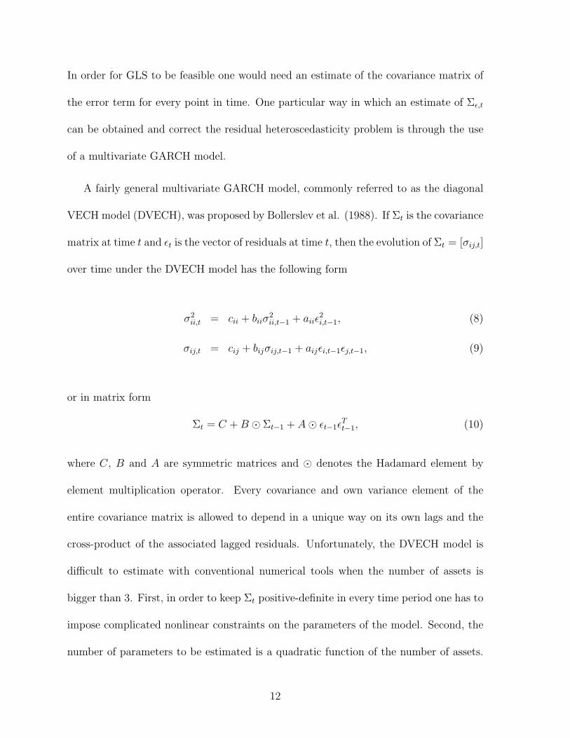
A fairly general multivariate GARCH model, commonly referred to as the diagonal

VECH model (DVECH), was proposed by Bollerslev et al. (1988). If Σt is the covariance

matrix at time t and εt is the vector of residuals at time t, then the evolution of Σt = [σij,t]

over time under the DVECH model has the following form

σ2ii,t = cii + biiσ

2ii,t−1 + aiiε

2i,t−1, (8)

σij,t = cij + bijσij,t−1 + aijεi,t−1εj,t−1, (9)

or in matrix form

Σt = C + B ¯ Σt−1 + A¯ εt−1εTt−1, (10)

where C, B and A are symmetric matrices and ¯ denotes the Hadamard element by

element multiplication operator. Every covariance and own variance element of the

entire covariance matrix is allowed to depend in a unique way on its own lags and the

cross-product of the associated lagged residuals. Unfortunately, the DVECH model is

difficult to estimate with conventional numerical tools when the number of assets is

bigger than 3. First, in order to keep Σt positive-definite in every time period one has to

impose complicated nonlinear constraints on the parameters of the model. Second, the

number of parameters to be estimated is a quadratic function of the number of assets.

12

These issues make this model difficult, if not impossible, to estimate for more than a

few assets. The BEKK model was introduced by Engle and Kroner (1995) in order

to address the first problem of positive-definiteness of the covariance matrix as well as

to provide a good approximation to the DVECH model in (10). Their model has the

following form:

Σt = C + BT Σt−1B + AT εt−1εTt−1A, (11)

where C is a positive-definite matrix. Notice that the two quadratic terms are positive-

definite by construction and, thus, Σt is guaranteed to remain positive definite.

Despite the obvious advantages it offers, the BEKK model has too many parameters

when systems larger than tri-variate are considered. In practice, parameter restrictions

are typically needed before numerical optimization algorithms can be used to estimate

this model in a feasible manner. The most common type of restriction is that the

matrices A and B are diagonal which results in the so-called diagonal BEKK model

(DBEKK). Occasionally, for larger systems, one has to constrain A and B even further

by assuming that they have the same parameter along their diagonals (scalar BEKK).

These practical considerations necessitate a sacrifice in terms of the generality of the

dynamics of the covariance matrix of returns over time. Another GARCH model that

has recently fallen out of fashion is the Bollerslev (1990) constant correlation GARCH

model (CCORR). In this model, the dynamics of the conditional variances are of the

same form as in (9) above. However, as the name of the model suggests, the covariances

are modeled as if the conditional correlation between the return series is the same in

13

every period:

σij,t = ρijσii,tσjj,t. (12)

A recent trend in the estimation of multivariate GARCH models has been the sep-

aration of the estimation process in stages. Initially, a series of univariate GARCH

models are fitted to every individual asset to estimate the parameters associated with

that asset’s own variance. Next, a separate procedure is used to estimate the param-

eters driving the covariances of asset returns. One example of this approach is Engle

(2002) which generalizes Bollerslev CCORR model. He introduces a dynamic conditional

correlation model in which the correlation between any two assets is an exponentially

smoothed function of past standardized residuals. In his model the correlation matrix

is guaranteed to be positive definite and is combined with a set of univariate GARCH

models for the individual assets variances to produce an estimate of the entire covariance

matrix of returns.

Another such model is introduced by Ledoit et al. (2003). In their model, they

also use a set of univariate GARCH models to estimate the own variance processes fist.

Then, for every covariance element they estimate a separate univariate GARCH process

much like the DVECH model above in (9). This procedure does not guarantee that

the parameter matrices A and B (as well as the covariance matrix Σt itself) will be

positive-definite. In a third and final step, Ledoit et al. (2003) show how to find the

“closest” positive-semidefinite A and B to the ones estimated in the previous stage in a

certain matrix norm.3 This GARCH model is essentially a diagonal VECH model first

proposed and estimated for a small set of assets in Bollerslev et al. (1988). It allows both

14

own variances and every covariance element to have a life of its own. For comparison,

the DCC model of Engle (2002) has 3 parameters that drive the entire evolution of the

correlation matrix over time. My motivation in choosing to use the model of Ledoit et

al. (2003) in this paper is, in part, based on its generality over the DCC model.

In this paper, I use the flexible multivariate GARCH model of Ledoit et al. (2003) in

order to estimate Σt, the joint covariance matrix of the three Fama-French factors and

the 25 size and book-to-market portfolios from Fama and French (1993,1996). Then I

compute the matrix of factor loadings Bt and use (7) to compute Σε,t, the covariance

matrix of the residuals in (1). Using this initial estimate of Σε,t, I employ a GLS proce-

dure to estimate θ = [α, β]. Then I compute the fitted residuals from (1) again. Next,

I use the flexible multivariate GARCH model and the multivariate CCORR GARCH

model directly on the fitted residuals from the previous step to produce another esti-

mate of Σε,t. Going back and forth, I repeat this process until the parameter vector θ

has converged. This should result in a feasible GLS (FGLS) estimate which converges

to the true GLS estimate under standard conditions. I adjust the standard errors of θ

to correct for the fact that an estimate of Σε,t is used in the FGLS procedure as well as

for any mis-specification in the dynamics of the multivariate GARCH model using the

results of Bollerslev and Wooldridge (1992).

15

III. Empirical Results

I use monthly simple excess returns for the 25 size and book-to-market sorted portfolios

from Fama and French (1993), the 30 industry-sorted portfolios as well as the MKT,

SMB, HML and UMD (Carhart (1997)) factor-mimicking portfolios for the sample period

July 1963 to December 1993.4

A. Data Description

Table 1 provides descriptive statistics for the 25 size and book-to-market portfolios.

The average excess returns are much larger for value (high book-to-market) than growth

portfolios (low book-to-market). The difference is statistically significant for all pairs

of such portfolios with the exception of the largest market capitalization one. This has

been referred to as the value premium in the literature. The return series also exhibit

significant departures from normality as indicated by the skewness and kurtosis tests.

There also appear to be significant first-order autocorrelations in particular for smaller

market capitalization stocks.

Insert Table 1 about here.

Summary statistics for the excess returns of the 30 industry portfolios are presented

in Table 2. There are fewer average excess returns that are statistically significant for

this set of assets as well as fewer deviations from the level of skewness for a normally

distributed variable. However, the kurtosis tests show that the distribution of monthly

excess returns is quite different from normal for all of the 30 assets. Finally, there are

16

fewer significant first-order autocorrelations for industry than size and book-to-market

portfolios’ excess returns.


B. Asset Pricing Implications

In this section, I compare the performance of several unconditional pricing models with

their conditional counterparts. Table 3 presents the OLS results for the unconditional

CAPM model. One notable feature of these results is that this model substantially

overprices growth stocks and underprices value stocks. The average absolute pricing

error is 28.76 basis points per month which translates into more than 3% per annum.

This is a substantial amount of mis-pricing. One popular measure of serial dependence

in fitted residuals is the Ljung-Box statistic from Ljung and Box (1978). It is defined as

a distributed lag function of the squared serial autocorrelations ρ2k of the fitted residuals

at lags k = 1, . . . ,m. Formally, their test statistic for the hypothesis of no ARCH effects

at lag m is computed in the following way:

Q(m) = T (T + 2)m∑

k=1

ρ2k

T − k, (13)

where T is the sample size. If a test of serial dependence in squared fitted residuals Q2(m)

is required, one should use ρ2k above where now the serial autocorrelation coefficient

refers to the squared fitted residuals.5 The values of the Ljung-Box diagnostic for serial

correlation at lag 1 (Q(1)) indicates that there are significant GARCH effects for a few

17

value and growth portfolio returns.


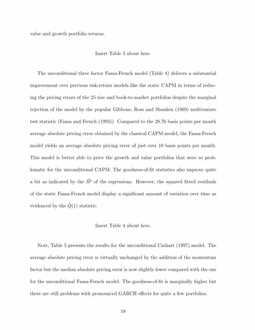
The unconditional three factor Fama-French model (Table 4) delivers a substantial

improvement over previous risk-return models like the static CAPM in terms of reduc-

ing the pricing errors of the 25 size and book-to-market portfolios despite the marginal

rejection of the model by the popular Gibbons, Ross and Shanken (1989) multivariate

test statistic (Fama and French (1993)). Compared to the 28.76 basis points per month

average absolute pricing error obtained by the classical CAPM model, the Fama-French

model yields an average absolute pricing error of just over 10 basis points per month.

This model is better able to price the growth and value portfolios that were so prob-

lematic for the unconditional CAPM. The goodness-of-fit statistics also improve quite

a bit as indicated by the R2 of the regressions. However, the squared fitted residuals

of the static Fama-French model display a significant amount of variation over time as

evidenced by the Q(1) statistic.


Next, Table 5 presents the results for the unconditional Carhart (1997) model. The

average absolute pricing error is virtually unchanged by the addition of the momentum

factor but the median absolute pricing error is now slightly lower compared with the one

for the unconditional Fama-French model. The goodness-of-fit is marginally higher but

there are still problems with pronounced GARCH effects for quite a few portfolios.

18


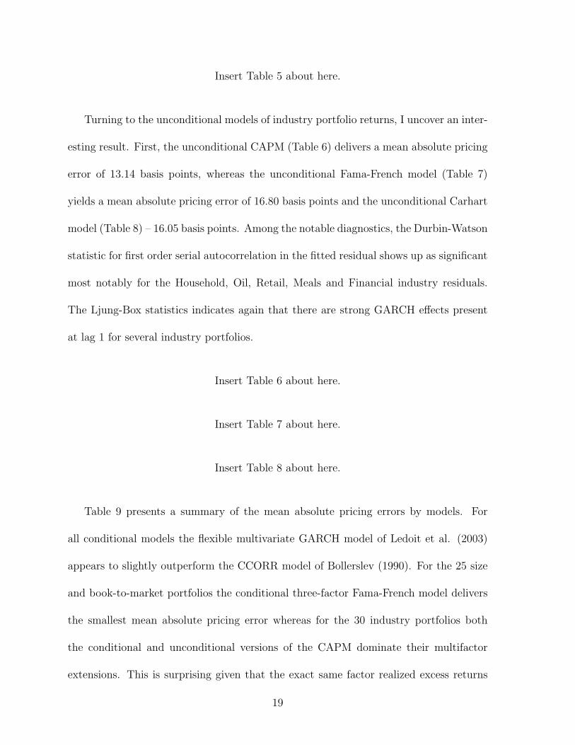
Turning to the unconditional models of industry portfolio returns, I uncover an inter-

esting result. First, the unconditional CAPM (Table 6) delivers a mean absolute pricing

error of 13.14 basis points, whereas the unconditional Fama-French model (Table 7)

yields a mean absolute pricing error of 16.80 basis points and the unconditional Carhart

model (Table 8) – 16.05 basis points. Among the notable diagnostics, the Durbin-Watson

statistic for first order serial autocorrelation in the fitted residual shows up as significant

most notably for the Household, Oil, Retail, Meals and Financial industry residuals.

The Ljung-Box statistics indicates again that there are strong GARCH effects present

at lag 1 for several industry portfolios.




Table 9 presents a summary of the mean absolute pricing errors by models. For

all conditional models the flexible multivariate GARCH model of Ledoit et al. (2003)

appears to slightly outperform the CCORR model of Bollerslev (1990). For the 25 size

and book-to-market portfolios the conditional three-factor Fama-French model delivers

the smallest mean absolute pricing error whereas for the 30 industry portfolios both

the conditional and unconditional versions of the CAPM dominate their multifactor

extensions. This is surprising given that the exact same factor realized excess returns

19

are used to model the realized returns of the two sets of assets. One possible explanation

for this inconsistency is that there are selection bias problems with the way the two sets

of returns are constructed (i.e. the 25 portfolios exclude firm returns with negative

book-to-market ratios). Another possibility is that the αis are not so much indications

of mis-pricing but are rather due to transactions costs and differential taxes on capital

gains and interest income.


Next, I present the results of several hypothesis tests to judge the importance of the

additional factors as well as the joint significance of the pricing errors. In Table 10, I

present the results for the 25 size and book-to-market portfolios. The joint hypothesis

that all the pricing errors are zero is strongly rejected for all three factor models in

both their conditional and unconditional form. Next, the hypothesis that both the SMB

and HML factors are jointly significant is rejected rather strongly for both multi-factor

models. Finally, the significance of the UMD factor as well as joint significance of all

three additional factors is very strongly rejected as well. It appears that the four-factor

Carhart (1997) model is the most preferred one if the size and book-to-market portfolios

are used as test assets. However, the results are quite different for the 30 industry

portfolios. As Table 11 reports, the joint hypothesis that the regression intercepts are

all zero cannot be rejected at any conventional levels both for the unconditional and

the conditional version of the CAPM. However, adding SMB and HML as well as UMD

completely reverses this result.

20



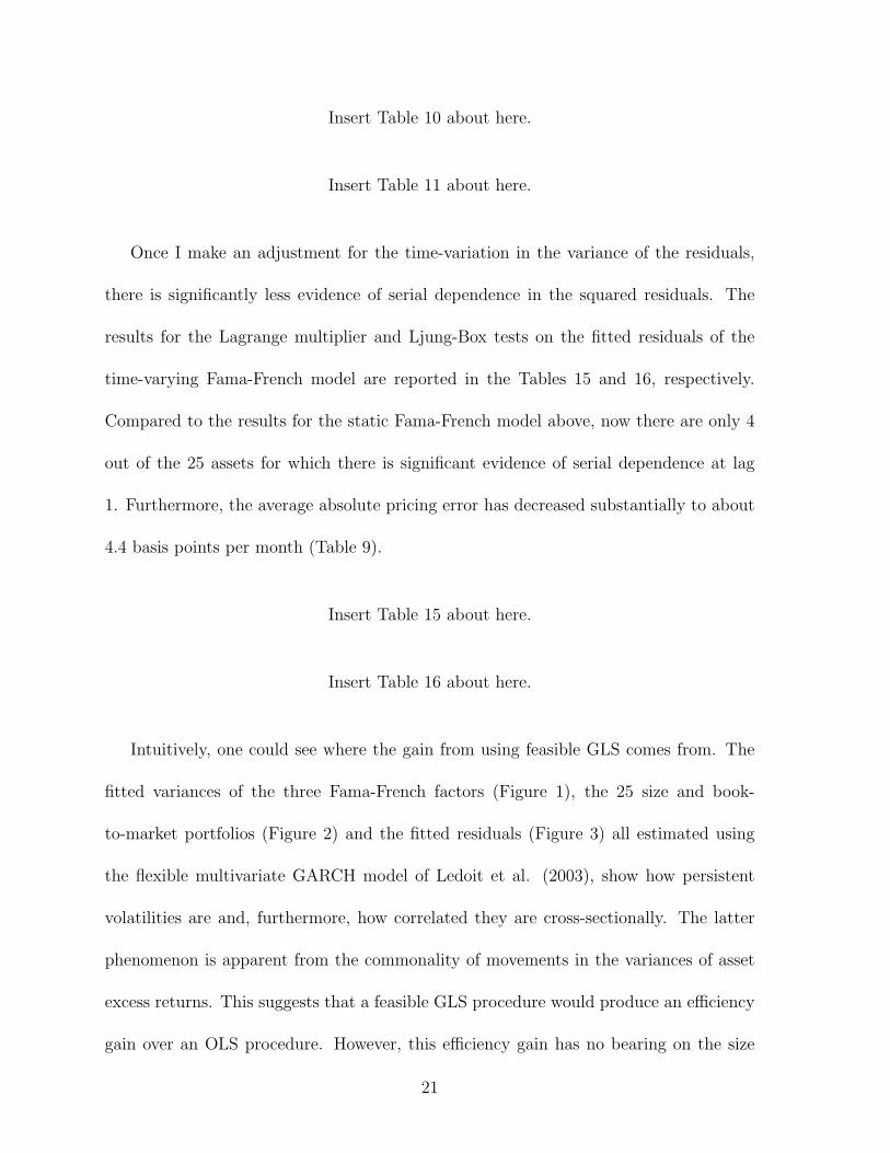
Once I make an adjustment for the time-variation in the variance of the residuals,

there is significantly less evidence of serial dependence in the squared residuals. The

results for the Lagrange multiplier and Ljung-Box tests on the fitted residuals of the

time-varying Fama-French model are reported in the Tables 15 and 16, respectively.

Compared to the results for the static Fama-French model above, now there are only 4

out of the 25 assets for which there is significant evidence of serial dependence at lag

1. Furthermore, the average absolute pricing error has decreased substantially to about

4.4 basis points per month (Table 9).



Intuitively, one could see where the gain from using feasible GLS comes from. The

fitted variances of the three Fama-French factors (Figure 1), the 25 size and book-

to-market portfolios (Figure 2) and the fitted residuals (Figure 3) all estimated using

the flexible multivariate GARCH model of Ledoit et al. (2003), show how persistent

volatilities are and, furthermore, how correlated they are cross-sectionally. The latter

phenomenon is apparent from the commonality of movements in the variances of asset

excess returns. This suggests that a feasible GLS procedure would produce an efficiency

gain over an OLS procedure. However, this efficiency gain has no bearing on the size

21

of the parameters only on their standard errors. Therefore, the improvement in the

pricing errors of the 25 portfolios is not a direct result of the FGLS. Rather, the FGLS

improves the precision of the estimates and it appears that the dynamic Fama-French

model has an even better ability to price the size and book-to-market portfolios than the

static one. However, for the industry portfolios the conditional as well as unconditional

CAPM outperform the multi-factor models as far as mean absolute pricing errors are

concerned. In an ideal world, it is inconceivable that having the right pricing model and

the right factors certain portfolios of individual securities will be priced a lot better than

others. Hence, there are several possible explanations for the conflicting empirical results

reported above. Either, the factors in these models are mis-specified or they leave a lot of

non-tradable assets out like human capital, for example. Another potential explanation

is that the models themselves are mis-specified. Finally, it is also quite possible that there

is something wrong with the way the portfolios are constructed, raising possible issues

about data-mining or selection/survivorship bias. This paper cannot resolve these issues

per se but can point towards the fact that the time-varying volatility models proposed

here go only part of the way towards explaining the puzzle documented above.

Insert Figure 1 about here.



22

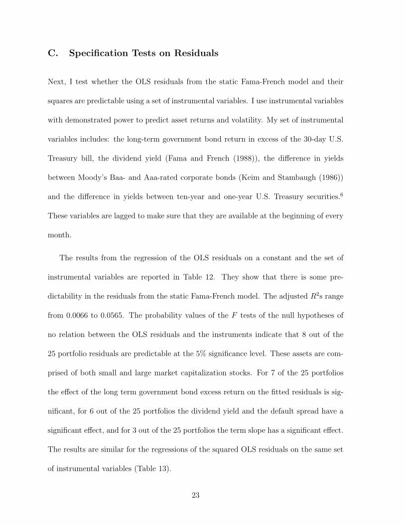
C. Specification Tests on Residuals

Next, I test whether the OLS residuals from the static Fama-French model and their

squares are predictable using a set of instrumental variables. I use instrumental variables

with demonstrated power to predict asset returns and volatility. My set of instrumental

variables includes: the long-term government bond return in excess of the 30-day U.S.

Treasury bill, the dividend yield (Fama and French (1988)), the difference in yields

between Moody’s Baa- and Aaa-rated corporate bonds (Keim and Stambaugh (1986))

and the difference in yields between ten-year and one-year U.S. Treasury securities.6

These variables are lagged to make sure that they are available at the beginning of every

month.

The results from the regression of the OLS residuals on a constant and the set of

instrumental variables are reported in Table 12. They show that there is some pre-

dictability in the residuals from the static Fama-French model. The adjusted R2s range

from 0.0066 to 0.0565. The probability values of the F tests of the null hypotheses of

no relation between the OLS residuals and the instruments indicate that 8 out of the

25 portfolio residuals are predictable at the 5% significance level. These assets are com-

prised of both small and large market capitalization stocks. For 7 of the 25 portfolios

the effect of the long term government bond excess return on the fitted residuals is sig-

nificant, for 6 out of the 25 portfolios the dividend yield and the default spread have a

significant effect, and for 3 out of the 25 portfolios the term slope has a significant effect.

The results are similar for the regressions of the squared OLS residuals on the same set

of instrumental variables (Table 13).

23



Now I turn to the results from the regression of the GLS residuals from the dynamic

Fama-French model and their squares on a constant and the instrumental variables.

These are presented in Tables 17 and 18, respectively. The regression results for the

GLS residuals show a slight improvement over the ones for the OLS residuals. The

adjusted R2 now range between 0.0040 and 0.0517. There is now one less asset for

which the excess long term government bond return has a significant return. There

are also three less assets for which the default premium has a significant effect. The

results for the squared GLS residuals show a slightly bigger improvement over the ones

for the squared OLS residuals. Now there are only 3 instead of 5 assets for which the

instruments have any significant ability to forecast the squared GLS residuals.



Overall, these predictability tests show that time-variation in the conditional factor

and residual covariance matrices can account for some but not all of the predictability

of asset returns.

24

D. Time Series Predictability of Factor Loadings

Finally, I investigate the time-variation of factor loadings Bt estimated at the first stage

of the dynamic Fama-French model with the flexible multivariate GARCH model of

Ledoit et al. (2003). Similar results obtain for the fitted factor loadings estimated using

the constant conditional correlation model of Bollerslev (1990) and are, therefore, not

reported here.7 I take the fitted values of βi, si and hi and regress them on a set of

instruments that includes a constant, the dividend yield, the term spread and a reces-

sion dummy variable which takes a value of 1 during recessions and zero otherwise.8 I

would like to emphasize that these time-varying exposures were not used explicitly in the

risk-return relations tested in the previous subsections because of numerical difficulties

associated with estimating such a complicated system even in stages let alone jointly.

Needless to say these fitted factor risk exposures are contemporaneous but noisy esti-

mates of the true factor exposures. They are provided here solely for completeness and

to highlight some potential problems and counter-intuitive behavior they exhibit over

the business cycle. These counter-indications may serve as a warning that we either have

mis-specified the factors, the GARCH model or both. Even worse, they may indicate

that our current understanding of macroeconomic variables and how they relate to each

as well as with financial risk measures over time is, at best, poor.

First, I report the results of the regressions of the estimated market factor loadings

ˆbetai on the instruments in Table 19. The market betas of the 25 portfolios appear to be

negatively correlated with the dividend yield. Of these, 18 have a significantly negative

coefficient on D/P . This suggests that a market-wide decrease in the dividend yield is

25

followed by increases in the exposure of the 25 Fama-French portfolios to the market risk

factor. Turning to the default premium, virtually all (23 out of 25) portfolios market

betas have negative coefficients on this instrumental variable. An increase in the term

premium has a significantly negative correlation with subsequent market betas for only

six portfolios without any pattern across the size and book-to-market dimension. The

recession dummy variable is significant for 18 of the 25 portfolios with a mostly negative

sign. The only exception are most growth portfolios which have a positive coefficient

on REC. This implies that the exposures of growth stocks to the market risk factor

increase during recessions while the exposures of value stocks decrease during recessions

regardless of market capitalization. The average R2 of these regressions across all 25

portfolios is quite high at 0.4113 with a minimum of 0.0167 for the large-cap median

book-to-market portfolio (FF53) and a maximum of 0.5841 for the small-cap median-

to-high book-to-market portfolio (FF14).


Next, I turn to the results of the regressions of the estimated SMB factor loadings si

on the instruments which are reported in Table 20. In this case, the dividend yield has

the opposite effect. Of the 18 significant D/P coefficients, 17 are positive. Similarly,

an increase in the default spread is followed by increases in SMB factor exposures for

22 of the 25 portfolios. An increase in the term spread has a small positive but mostly

insignificant effect on sis. The recession indicator has mixed effects on the SMB fac-

tor loadings. The coefficient of the REC instrument has a negative sign for mid-cap

portfolios and a positive sign for large-cap value and growth portfolios. Overall, the

26

signs of D/P , DEF and TERM coefficients for the SMB factor are virtually exactly the

opposite ones of those for the market factor. These results suggest that increases in the

aggregate dividend yield as well as increases in the default and term spreads are followed

by increases in assets exposures to the SMB factor and decreases in assets exposures to

the market factor. The average R2 of these regression over all 25 portfolios is 0.2011 and

is about half as large as the one from the fitted market betas regressions. The smallest

R2 in this case is 0.0239 for the small-cap growth portfolio (FF11) and the highest R2

is 0.3193 for the medium-cap value portfolio (FF35).


Lastly, I report the results of the regressions of the HML factor loadings hi in Table 21.

In this case, an increase in the market dividend yield is subsequently followed by a

decrease of the HML exposures of value stocks and an increase of the HML exposures

of growth stocks. The statistical significance of these results is stronger for stocks with

larger market capitalizations. The impact of an increase in the default spread is negative

and significant for almost all of the 25 portfolios as was the case for the market factor

exposures. The term spread appears to have a positive impact on the HML exposures of

value stocks and a negative impact on the HML exposures of growth stocks. However,

this result has to be treated with caution since very few of the TERM coefficients are

significant. Finally, the coefficients of the recession dummy variable suggest that HML

exposures increase for value stocks and decrease for growth stocks when the economy

is in a recession. The average R2 of these regressions is 0.1105 with a minimum of

0.0107 for the median-to-large capitalization growth portfolio (FF41) and a maximum

27

of 0.2655 for the median-cap value portfolio (FF35). The average goodness-of-fit of the

HML regressions is half as big as the average one of the SMB beta regressions and only

a quarter of the one from the market beta regressions. These results suggest that if

the Fama-French factor loadings are to be modelled as a reduced form linear function

of lagged instrumental variables, this approach will be more powerful for market betas,

less powerful for SMB betas and least powerful for HML betas, at least for this set of

test assets and within the sample period under consideration. This casts some doubt on

these popular modeling approaches of time-varying factor exposures.


IV. Conclusion

In this paper, I adapt a recently developed flexible multivariate GARCH model to gener-

alize the well known and, by now, standard Fama and French (1993) and Carhart (1997)

models by incorporating time varying idiosyncratic volatility. I initially replicate the re-

sults of the static Fama and French (1993) model for the 25 size and book-to-market

portfolios and analyze the residuals to check whether they satisfy the assumptions that

validate the use of OLS in their paper. I show that there is one serious statistical problem

with the static Fama-French model. The squared fitted residuals from their regressions

exhibit very substantial serial correlation which violates the homoscedasticity assump-

tion of OLS. This is evidence of what has become known as a GARCH effect in the

literature. The presence of GARCH effects in the size and book-to-market portfolios is

28

not surprising as most financial returns series that have been examined exhibit GARCH

effects. However, this suggests an avenue for improvement of the static Fama-French

model by allowing the volatility of factor and asset returns to change over time. One

parsimonious way to achieve this goal is to incorporate a multivariate GARCH model

into the linear three factor risk-return relation of Fama and French (1993) and the lin-

ear four-factor Carhart (1997) model. To this end, I use a multivariate GARCH model

proposed by Ledoit et al. (2003) as well as a two-stage constant correlation GARCH

model (Bollerslev (1990)).

These new dynamic Fama-French and Carhart models appear to do a very good job

at eliminating the GARCH effects present in the size and book-to-market as well as

industry portfolios. The serial correlation in the squared fitted residuals is substantially

reduced as evidenced by the Lagrange multiplier and the Ljung-Box test. Moreover,

the dynamic models produce a dramatic improvement in the pricing errors of the 25

size and book-to-market and 30 industry portfolios. In the static model of Fama and

French (1993), the average absolute pricing error is 10 basis points per month. Once

I adjust the estimation process to allow for the time-variation of the volatility of the

residuals, I obtain an average absolute pricing error of 4.5 basis points per month. This

is a reduction in excess of 50% compared to the results of the static Fama-French model.

For the industry portfolios, the improvement is even bigger – from just over 13% for the

unconditional CAPM down to 4% for the conditional CAPM. However, I am unable to

identify a single risk-return relationship that prices both sets of portfolios reasonably

well.

29

In addition, I investigate whether time variation of the conditional second moments

of the Fama-French factors and their 25 portfolios can account for the predictability

of asset returns. I find that this time variation explains only a small portion of the

predictable variation in the size and book-to-market portfolio returns. After controlling

for a majority of the documented GARCH effects, the residuals from the dynamic Fama-

French model are still forecastable using popular instrumental variables like the dividend

yield, the default spread and the term spread.

Finally, I characterize the correlations between several instrumental variables and the

assets’ factor loadings in the framework of the proposed dynamic Fama-French model.

I show that, increases in the market dividend yield, the default spread and the term

spread are followed by a decrease in market betas. This result is at odds with the results

of Shanken (1990). It raises a red flag about the modeling of factor loadings as linear

combinations of instrumental variables without investigating the economic forces that

might be driving the actual relationship between instruments and factor loadings. At

the same time, the same changes in these instrumental variables are followed by the

exact opposite changes in the SMB betas. This result conforms better with economic

intuition. I also document important business cycle effects in the time variation of

the factor loadings. Market betas of growth stocks tend to increase during recessions

while market betas of value stocks tend to decrease during recessions. Loadings on the

HML factor, however, increase for value stocks and decrease for growth stocks during

recessions. Unlike the former result about market betas, the latter result about HML

exposures conforms nicely with the empirical fact that average returns of value stocks

30

are higher than average returns of growth stocks, particularly so during recessions than

during economic booms. The net result of these effects varies widely from an overall

increase to an overall decrease in the total amount of systematic portfolio risk depending

on the exact values of the instrumental variables. Overall, the ad hoc analysis of the

time-variation of the estimated factor loadings suggests that there may be a variety of

forces at play and merits a more in-depth study. Such an investigation is beyond the

scope of this paper and is left for future study.

A potential extension of these dynamic multi-factor models would be to incorporate

asymmetric volatility effects (Engle and Ng (1993)) into the flexible multivariate GARCH

part of the model. This may mitigate even further the GARCH effects documented

above. Furthermore, it would be instructive to investigate whether the good in-sample

pricing performance of the proposed models persists in out-of-sample dynamic tests. It

is left for further research to determine the effects of these extensions on the performance

of the dynamic Fama-French and Carhart models proposed in this paper.

31

Footnotes

1See Fama and French (1993) for more details on the complete set of sample selection

criteria as well as the exclusion of negative BM stocks, etc.

2First-pass estimates of the time-varying factor exposures exhibit small in-sample

covariances with the realized factor returns indicating that the Jagannathan and Wang

(1997) correction in this case will be small which is why I have omitted this correction

from the analysis that is to follow. Details are available from the author upon request.

3I am grateful to P. Santa-Clara for providing the computer code used in Ledoit et

al. (2003).

4I obtained the return series data from K. French’s website and I am grateful to him

for providing it publicly.

5Tims and Mahieu (2003) refer to this statistic as the McLeod and Li (1983) test.

6The Treasury yields are from the CRSP Treasury Bill Term Structure files. The

dividend yield on the CRSP value-weighted index of NYSE and AMEX stocks. The

long term government bond returns are from Ibbotson Associates Stocks, Bonds, Bills

and Inflation 1998 Yearbook.

7Details are available from the author upon request.

8The dates for troughs and peaks that determine recession periods are taken from

the National Bureau of Economic Research.

32

Bibliography

[1] Banz, R., 1981, The Relationship Between Return and Market Value of Common

Stocks, Journal of Financial Economics 9, 3–18.

[2] Basu, S., 1983, The Relationship Between Earnings’ Yield, Market Value and Re-

turn for NYSE Common Stocks: Further Evidence, Journal of Financial Economics,

12, 129–156.

[3] Berk, J., R. Green and V. Naik, 1999, Optimal Investment, Growth Options and

Security Returns, Journal of Finance 54, 1153–1607.

[4] Black, F., M. C. Jensen and M. Scholes, 1972, The Capital Asset Pricing Model:

Some Empirical Tests, in M. Jensen (ed.) Studies in the Theory of Capital Markets

(Praeger).

[5] Bollerslev, T., 1990, Modelling the Coherence in Short-Run Nominal Exchange

Rates: A Multivariate Generalized ARCH Model, Review of Economics and Statis-

tics 72, 498–505.

33

[6] Bollerslev, T. and J. Wooldridge, 1992, Quasi-Maximum Likelihood Estimation and

Inference in Dynamic Models with Time-Varying Covariances, Econometric Review

11, 143–172.

[7] Bolleslev, T., R. F. Engle and J. Wooldridge, 1988, Capital Asset Pricing Model

with Time-Varying Covariances, Journal of Political Economy 96, 116–131.

[8] Carhart, M. M., 1997, On Persistence in Mutual Fund Performance, Journal of

Finance 52, 57–82.

[9] Chung, Y. P., H. Johnson and M. J. Schill, 2001, Asset Pricing When Returns

are Non-Normal: Fama-French Factors vs. Higher-Order Systematic Co-Moments,

Working paper, University of California, Riverside.

[10] Cohen, R. B. and C. K. Polk, 1995, COMPUSTAT Selection Bias in Tests of the

Sharpe-Lintner-Black CAPM, Working paper, University of Chicago.

[11] Daniel, K. and S. Titman, 1997, Evidence on the Characteristics of Cross Sectional

Variation in Stock Returns, Journal of Finance 52, 1–34.

[12] Davis, J. L., 1994, The Cross-Section of Realized Stock Returns: The pre-

COMPUSTAT Evidence, Journal of Finance 50, 1579–1593.

[13] Engle, R. F., 2002, Dynamic Conditional Correlation – A Simple Class of Multi-

variate GARCH Models, Journal of Business and Economic Statistics Vol. 17, No.

5.

34

[14] Engle, R. F. and K. F. Kroner, 1995, Multivariate Simultaneous GARCH, Econo-

metric Theory 11, 122-150.

[15] Engle, R. F. and V. K. Ng, 1993, Measuring and Testing the Impact of News on

Volatility, Journal of Finance 48, 1749–1778.

[16] Fama, E. F. and K. R. French, 1988, Dividend Yields and Expected Returns on

Stocks and Bonds, Journal of Financial Economics 22, 3–25.

[17] Fama, E. F. and K. R. French, 1992, The Cross-Section of Expected Stock Returns,

Journal of Finance 47, 427–465.

[18] Fama, E. F. and K. R. French, 1993, Common Risk Factors in the Returns on

Stocks and Bonds, Journal of Financial Economics 33, 3–56.

[19] Fama, E. F. and K. R. French, 1996, Multifactor Explanations of Asset Pricing

Anomalies, Journal of Finance 51, 55–84.

[20] Fama, E. F. and J. D. MacBeth, 1973, Risk, Return and Equilibrium: Empirical

Tests, Journal of Political Economy 81, 607–636.

[21] Gibbons, M. R., S. A. Ross and J. Shanken, 1989, A Test of the Efficiency of a

Given Portfolio, Econometrica 57, 1121–1152.

[22] Gomes, J., L. Kogan and L. Zhang, 2003, Equilibrium Cross-Section of Returns,

Journal of Political Economy 111, 693–732.

[23] Jagannathan, R. and Z. Wang, 1997, The Conditional CAPM and the Cross-Section

of Expected Returns, Journal of Finance 51, 3–53.

35

[24] Jegadeesh, N. and S. Titman, 1993, Returns to Buying Winners and Selling Losers:

Implications for Stock Market Efficiency, Journal of Finance 48, 65–91.

[25] Keim, D. B. and R. F. Stambaugh, 1986, Predicting Returns in the Stock and Bond

Markets, Journal of Financial Economics 17, 357–390.

[26] Kogan, L., 2001, An Equilibrium Model of Irreversible Investment, Journal of Fi-

nancial Economics 62, 201–245.

[27] Kogan, L., 2004, Asset Prices and Real Investment, Journal of Financial Economics

73, 411–432.

[28] Kothari, S. P., J. Shanken and R. Sloan, 1995, Another Look at the Cross-Section

of Expected Returns, Journal of Finance 50, 185–224.

[29] Lakonishok, J., A. Schleifer and R. W. Vishny, 1994, Contrarian Investment, Ex-

trapolation, and Risk, Journal of Finance 49, 1541–1578.

[30] Ledoit, O., P. Santa-Clara and M. Wolf, 2003, Flexible Multivariate GARCH Mod-

eling With an Application to International Stock Markets, Review of Economics

and Statistics 85, Issue 3, 735–747.

[31] Lintner, J., 1965, The Valuation of Risky Assets and the Selection of Risky Invest-

ments in Stock Portfolios and Capital Budgets, Review of Economics and Statistics

47, 13–37.

[32] Lo, A., and A. C. MacKinlay, 1990, Data Snooping Biases in Tests of Financial

Asset Pricing Models, Review of Financial Studies 3, 431–468.

36

[33] Ljung, G. and G. Box, 1978, On a Measure of Lack of Fit in Time Series Models,

Biometrika 65, 297–303.

[34] McLeod, A. L. and W. K. Li, 1983, Diagnostic Checking ARMA Time Series Models

Using Squared-Residual Autocorrelations, Journal of Time Series Analysis 4, 269–

273.

[35] Moskowitz, T. J., 2003, An Analysis of Covariance Risk and Pricing Anomalies,

Review of Financial Studies 16, No. 2, pp. 417–457.

[36] Petkova, R., 2006, Do the Fama-French Factors Proxy for Innovations in Predictive

Variables?, Journal of Finance 61, 581–612.

[37] Petkova, R. and L. Zhang, 2005, Is Value Riskier than Growth?, Journal of Finan-

cial Economics 78, 187–202.

[38] Shanken, J., 1990, Intertemporal Asset Pricing: An Empirical Investigation, Jour-

nal of Econometrics 45, 99-120.

[39] Sharpe, W. F., 1964, Capital Asset Prices: A Theory of Market Equilibrium under

Conditions of Risk, Journal of Finance 19, 425–442.

[40] Tims, B. and R. Mahieu, 2003, International Portfolio Choice: A Spanning Ap-

proach, Working Paper, Rotterdam School of Management, Erasmus University.

37

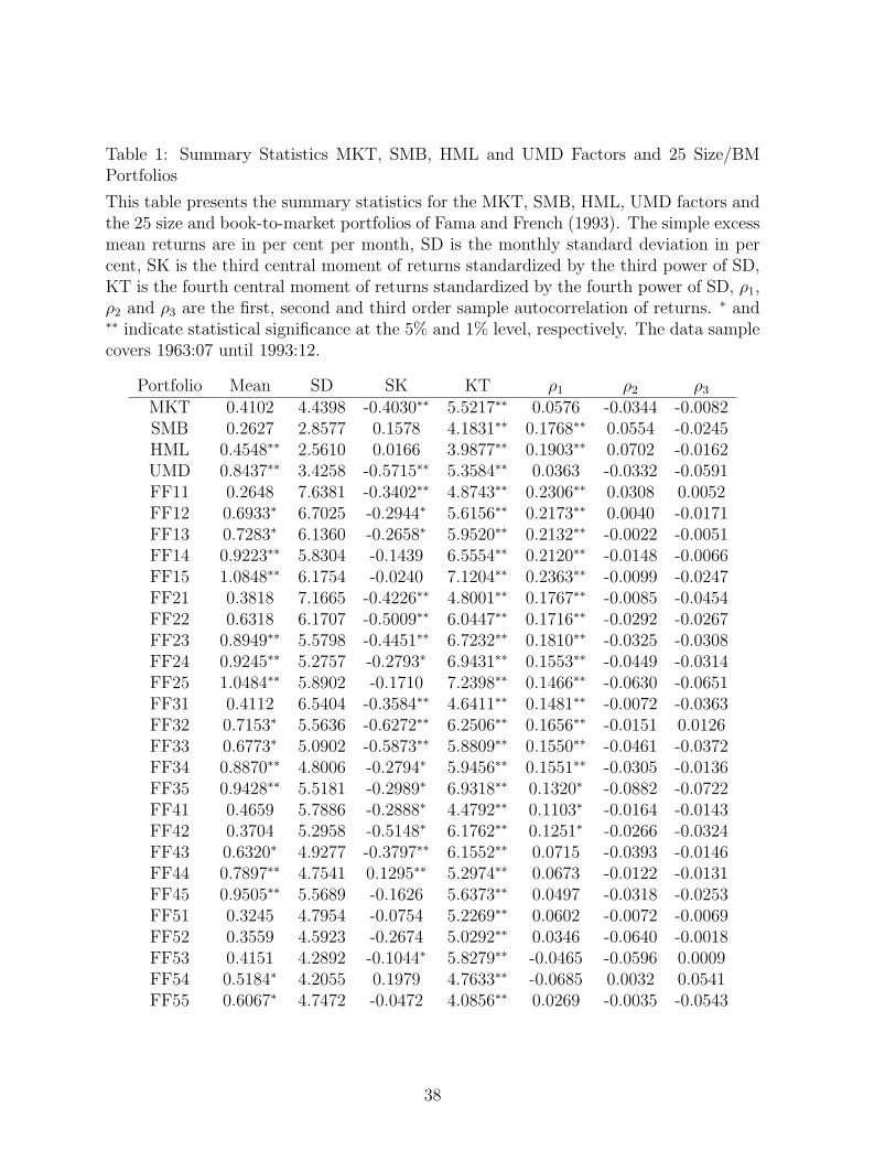
Table 1: Summary Statistics MKT, SMB, HML and UMD Factors and 25 Size/BMPortfolios

This table presents the summary statistics for the MKT, SMB, HML, UMD factors andthe 25 size and book-to-market portfolios of Fama and French (1993). The simple excessmean returns are in per cent per month, SD is the monthly standard deviation in percent, SK is the third central moment of returns standardized by the third power of SD,KT is the fourth central moment of returns standardized by the fourth power of SD, ρ1,ρ2 and ρ3 are the first, second and third order sample autocorrelation of returns. ∗ and∗∗ indicate statistical significance at the 5% and 1% level, respectively. The data samplecovers 1963:07 until 1993:12.

Portfolio Mean SD SK KT ρ1 ρ2 ρ3

MKT 0.4102 4.4398 -0.4030∗∗ 5.5217∗∗ 0.0576 -0.0344 -0.0082SMB 0.2627 2.8577 0.1578 4.1831∗∗ 0.1768∗∗ 0.0554 -0.0245HML 0.4548∗∗ 2.5610 0.0166 3.9877∗∗ 0.1903∗∗ 0.0702 -0.0162UMD 0.8437∗∗ 3.4258 -0.5715∗∗ 5.3584∗∗ 0.0363 -0.0332 -0.0591FF11 0.2648 7.6381 -0.3402∗∗ 4.8743∗∗ 0.2306∗∗ 0.0308 0.0052FF12 0.6933∗ 6.7025 -0.2944∗ 5.6156∗∗ 0.2173∗∗ 0.0040 -0.0171FF13 0.7283∗ 6.1360 -0.2658∗ 5.9520∗∗ 0.2132∗∗ -0.0022 -0.0051FF14 0.9223∗∗ 5.8304 -0.1439 6.5554∗∗ 0.2120∗∗ -0.0148 -0.0066FF15 1.0848∗∗ 6.1754 -0.0240 7.1204∗∗ 0.2363∗∗ -0.0099 -0.0247FF21 0.3818 7.1665 -0.4226∗∗ 4.8001∗∗ 0.1767∗∗ -0.0085 -0.0454FF22 0.6318 6.1707 -0.5009∗∗ 6.0447∗∗ 0.1716∗∗ -0.0292 -0.0267FF23 0.8949∗∗ 5.5798 -0.4451∗∗ 6.7232∗∗ 0.1810∗∗ -0.0325 -0.0308FF24 0.9245∗∗ 5.2757 -0.2793∗ 6.9431∗∗ 0.1553∗∗ -0.0449 -0.0314FF25 1.0484∗∗ 5.8902 -0.1710 7.2398∗∗ 0.1466∗∗ -0.0630 -0.0651FF31 0.4112 6.5404 -0.3584∗∗ 4.6411∗∗ 0.1481∗∗ -0.0072 -0.0363FF32 0.7153∗ 5.5636 -0.6272∗∗ 6.2506∗∗ 0.1656∗∗ -0.0151 0.0126FF33 0.6773∗ 5.0902 -0.5873∗∗ 5.8809∗∗ 0.1550∗∗ -0.0461 -0.0372FF34 0.8870∗∗ 4.8006 -0.2794∗ 5.9456∗∗ 0.1551∗∗ -0.0305 -0.0136FF35 0.9428∗∗ 5.5181 -0.2989∗ 6.9318∗∗ 0.1320∗ -0.0882 -0.0722FF41 0.4659 5.7886 -0.2888∗ 4.4792∗∗ 0.1103∗ -0.0164 -0.0143FF42 0.3704 5.2958 -0.5148∗ 6.1762∗∗ 0.1251∗ -0.0266 -0.0324FF43 0.6320∗ 4.9277 -0.3797∗∗ 6.1552∗∗ 0.0715 -0.0393 -0.0146FF44 0.7897∗∗ 4.7541 0.1295∗∗ 5.2974∗∗ 0.0673 -0.0122 -0.0131FF45 0.9505∗∗ 5.5689 -0.1626 5.6373∗∗ 0.0497 -0.0318 -0.0253FF51 0.3245 4.7954 -0.0754 5.2269∗∗ 0.0602 -0.0072 -0.0069FF52 0.3559 4.5923 -0.2674 5.0292∗∗ 0.0346 -0.0640 -0.0018FF53 0.4151 4.2892 -0.1044∗ 5.8279∗∗ -0.0465 -0.0596 0.0009FF54 0.5184∗ 4.2055 0.1979 4.7633∗∗ -0.0685 0.0032 0.0541FF55 0.6067∗ 4.7472 -0.0472 4.0856∗∗ 0.0269 -0.0035 -0.0543

38

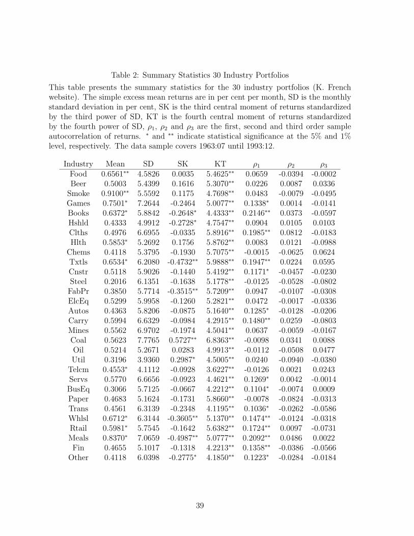
Table 2: Summary Statistics 30 Industry Portfolios

This table presents the summary statistics for the 30 industry portfolios (K. Frenchwebsite). The simple excess mean returns are in per cent per month, SD is the monthlystandard deviation in per cent, SK is the third central moment of returns standardizedby the third power of SD, KT is the fourth central moment of returns standardizedby the fourth power of SD, ρ1, ρ2 and ρ3 are the first, second and third order sampleautocorrelation of returns. ∗ and ∗∗ indicate statistical significance at the 5% and 1%level, respectively. The data sample covers 1963:07 until 1993:12.

Industry Mean SD SK KT ρ1 ρ2 ρ3

Food 0.6561∗∗ 4.5826 0.0035 5.4625∗∗ 0.0659 -0.0394 -0.0002Beer 0.5003 5.4399 0.1616 5.3070∗∗ 0.0226 0.0087 0.0336

Smoke 0.9100∗∗ 5.5592 0.1175 4.7698∗∗ 0.0483 -0.0079 -0.0495Games 0.7501∗ 7.2644 -0.2464 5.0077∗∗ 0.1338∗ 0.0014 -0.0141Books 0.6372∗ 5.8842 -0.2648∗ 4.4333∗∗ 0.2146∗∗ 0.0373 -0.0597Hshld 0.4333 4.9912 -0.2728∗ 4.7547∗∗ 0.0904 0.0105 0.0103Clths 0.4976 6.6955 -0.0335 5.8916∗∗ 0.1985∗∗ 0.0812 -0.0183Hlth 0.5853∗ 5.2692 0.1756 5.8762∗∗ 0.0083 0.0121 -0.0988

Chems 0.4118 5.3795 -0.1930 5.7075∗∗ -0.0015 -0.0625 0.0624Txtls 0.6534∗ 6.2080 -0.4732∗∗ 5.9888∗∗ 0.1947∗∗ 0.0224 0.0595Cnstr 0.5118 5.9026 -0.1440 5.4192∗∗ 0.1171∗ -0.0457 -0.0230Steel 0.2016 6.1351 -0.1638 5.1778∗∗ -0.0125 -0.0528 -0.0802FabPr 0.3850 5.7714 -0.3515∗∗ 5.7209∗∗ 0.0947 -0.0107 -0.0308ElcEq 0.5299 5.9958 -0.1260 5.2821∗∗ 0.0472 -0.0017 -0.0336Autos 0.4363 5.8206 -0.0875 5.1640∗∗ 0.1285∗ -0.0128 -0.0206Carry 0.5994 6.6329 -0.0984 4.2915∗∗ 0.1480∗∗ 0.0259 -0.0803Mines 0.5562 6.9702 -0.1974 4.5041∗∗ 0.0637 -0.0059 -0.0167Coal 0.5623 7.7765 0.5727∗∗ 6.8363∗∗ -0.0098 0.0341 0.0088Oil 0.5214 5.2671 0.0283 4.9913∗∗ -0.0112 -0.0508 0.0477Util 0.3196 3.9360 0.2987∗ 4.5005∗∗ 0.0240 -0.0940 -0.0380

Telcm 0.4553∗ 4.1112 -0.0928 3.6227∗∗ -0.0126 0.0021 0.0243Servs 0.5770 6.6656 -0.0923 4.4621∗∗ 0.1269∗ 0.0042 -0.0014BusEq 0.3066 5.7125 -0.0667 4.2212∗∗ 0.1104∗ -0.0074 0.0009Paper 0.4683 5.1624 -0.1731 5.8660∗∗ -0.0078 -0.0824 -0.0313Trans 0.4561 6.3139 -0.2348 4.1195∗∗ 0.1036∗ -0.0262 -0.0586Whlsl 0.6712∗ 6.3144 -0.3605∗∗ 5.1370∗∗ 0.1474∗∗ -0.0124 -0.0318Rtail 0.5981∗ 5.7545 -0.1642 5.6382∗∗ 0.1724∗∗ 0.0097 -0.0731Meals 0.8370∗ 7.0659 -0.4987∗∗ 5.0777∗∗ 0.2092∗∗ 0.0486 0.0022Fin 0.4655 5.1017 -0.1318 4.2213∗∗ 0.1358∗∗ -0.0386 -0.0566

Other 0.4118 6.0398 -0.2775∗ 4.1850∗∗ 0.1223∗ -0.0284 -0.0184

39

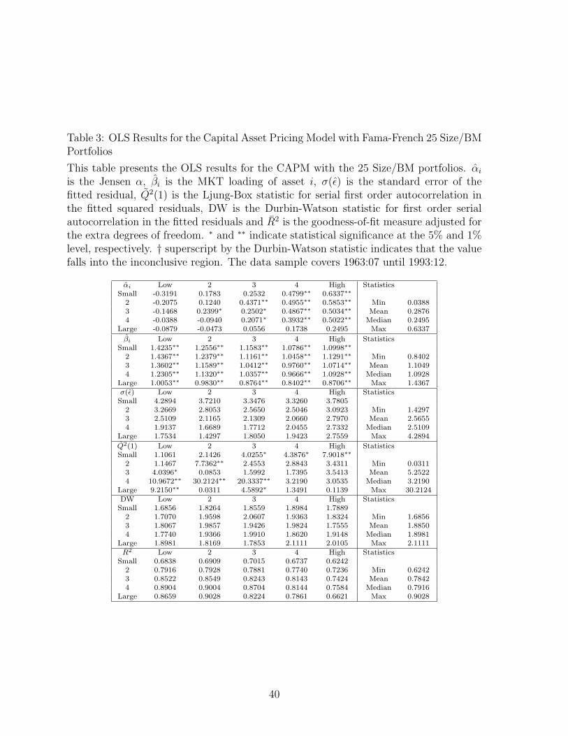
Table 3: OLS Results for the Capital Asset Pricing Model with Fama-French 25 Size/BMPortfolios

This table presents the OLS results for the CAPM with the 25 Size/BM portfolios. αi

is the Jensen α, βi is the MKT loading of asset i, σ(ε) is the standard error of thefitted residual, Q2(1) is the Ljung-Box statistic for serial first order autocorrelation inthe fitted squared residuals, DW is the Durbin-Watson statistic for first order serialautocorrelation in the fitted residuals and R2 is the goodness-of-fit measure adjusted forthe extra degrees of freedom. ∗ and ∗∗ indicate statistical significance at the 5% and 1%level, respectively. † superscript by the Durbin-Watson statistic indicates that the valuefalls into the inconclusive region. The data sample covers 1963:07 until 1993:12.

αi Low 2 3 4 High StatisticsSmall -0.3191 0.1783 0.2532 0.4799∗∗ 0.6337∗∗

2 -0.2075 0.1240 0.4371∗∗ 0.4955∗∗ 0.5853∗∗ Min 0.03883 -0.1468 0.2399∗ 0.2502∗ 0.4867∗∗ 0.5034∗∗ Mean 0.28764 -0.0388 -0.0940 0.2071∗ 0.3932∗∗ 0.5022∗∗ Median 0.2495

Large -0.0879 -0.0473 0.0556 0.1738 0.2495 Max 0.6337

βi Low 2 3 4 High StatisticsSmall 1.4235∗∗ 1.2556∗∗ 1.1583∗∗ 1.0786∗∗ 1.0998∗∗

2 1.4367∗∗ 1.2379∗∗ 1.1161∗∗ 1.0458∗∗ 1.1291∗∗ Min 0.84023 1.3602∗∗ 1.1589∗∗ 1.0412∗∗ 0.9760∗∗ 1.0714∗∗ Mean 1.10494 1.2305∗∗ 1.1320∗∗ 1.0357∗∗ 0.9666∗∗ 1.0928∗∗ Median 1.0928

Large 1.0053∗∗ 0.9830∗∗ 0.8764∗∗ 0.8402∗∗ 0.8706∗∗ Max 1.4367σ(ε) Low 2 3 4 High StatisticsSmall 4.2894 3.7210 3.3476 3.3260 3.7805

2 3.2669 2.8053 2.5650 2.5046 3.0923 Min 1.42973 2.5109 2.1165 2.1309 2.0660 2.7970 Mean 2.56554 1.9137 1.6689 1.7712 2.0455 2.7332 Median 2.5109

Large 1.7534 1.4297 1.8050 1.9423 2.7559 Max 4.2894

Q2(1) Low 2 3 4 High StatisticsSmall 1.1061 2.1426 4.0255∗ 4.3876∗ 7.9018∗∗

2 1.1467 7.7362∗∗ 2.4553 2.8843 3.4311 Min 0.03113 4.0396∗ 0.0853 1.5992 1.7395 3.5413 Mean 5.25224 10.9672∗∗ 30.2124∗∗ 20.3337∗∗ 3.2190 3.0535 Median 3.2190

Large 9.2150∗∗ 0.0311 4.5892∗ 1.3491 0.1139 Max 30.2124DW Low 2 3 4 High Statistics

Small 1.6856 1.8264 1.8559 1.8984 1.78892 1.7070 1.9598 2.0607 1.9363 1.8324 Min 1.68563 1.8067 1.9857 1.9426 1.9824 1.7555 Mean 1.88504 1.7740 1.9366 1.9910 1.8620 1.9148 Median 1.8981

Large 1.8981 1.8169 1.7853 2.1111 2.0105 Max 2.1111R2 Low 2 3 4 High Statistics


Large 0.8659 0.9028 0.8224 0.7861 0.6621 Max 0.9028

40

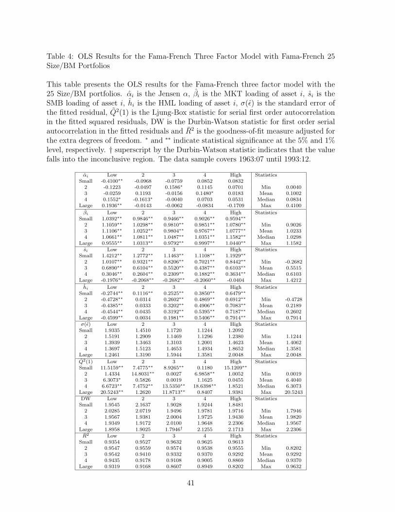
Table 4: OLS Results for the Fama-French Three Factor Model with Fama-French 25Size/BM Portfolios

This table presents the OLS results for the Fama-French three factor model with the25 Size/BM portfolios. αi is the Jensen α, βi is the MKT loading of asset i, si is theSMB loading of asset i, hi is the HML loading of asset i, σ(ε) is the standard error ofthe fitted residual, Q2(1) is the Ljung-Box statistic for serial first order autocorrelationin the fitted squared residuals, DW is the Durbin-Watson statistic for first order serialautocorrelation in the fitted residuals and R2 is the goodness-of-fit measure adjusted forthe extra degrees of freedom. ∗ and ∗∗ indicate statistical significance at the 5% and 1%level, respectively. † superscript by the Durbin-Watson statistic indicates that the valuefalls into the inconclusive region. The data sample covers 1963:07 until 1993:12.

αi Low 2 3 4 High StatisticsSmall -0.4100∗∗ -0.0968 -0.0759 0.0852 0.0832

2 -0.1223 -0.0497 0.1586∗ 0.1145 0.0701 Min 0.00403 -0.0259 0.1193 -0.0156 0.1480∗ 0.0183 Mean 0.10024 0.1552∗ -0.1613∗ -0.0040 0.0703 0.0531 Median 0.0834

Large 0.1936∗∗ -0.0143 -0.0062 -0.0834 -0.1709 Max 0.4100


2 1.1059∗∗ 1.0298∗∗ 0.9810∗∗ 0.9851∗∗ 1.0780∗∗ Min 0.90263 1.1106∗∗ 1.0252∗∗ 0.9804∗∗ 0.9767∗∗ 1.0777∗∗ Mean 1.02334 1.0661∗∗ 1.0811∗∗ 1.0487∗∗ 1.0351∗∗ 1.1582∗∗ Median 1.0298

Large 0.9555∗∗ 1.0313∗∗ 0.9792∗∗ 0.9997∗∗ 1.0440∗∗ Max 1.1582si Low 2 3 4 High Statistics

Small 1.4212∗∗ 1.2772∗∗ 1.1463∗∗ 1.1108∗∗ 1.1929∗∗2 1.0107∗∗ 0.9321∗∗ 0.8206∗∗ 0.7021∗∗ 0.8442∗∗ Min -0.26823 0.6890∗∗ 0.6104∗∗ 0.5520∗∗ 0.4387∗∗ 0.6103∗∗ Mean 0.55154 0.3046∗∗ 0.2604∗∗ 0.2309∗∗ 0.1882∗∗ 0.3634∗∗ Median 0.6103

Large -0.1976∗∗ -0.2068∗∗ -0.2682∗∗ -0.2060∗∗ -0.0404 Max 1.4212

hi Low 2 3 4 High StatisticsSmall -0.2744∗∗ 0.1116∗∗ 0.2525∗∗ 0.3850∗∗ 0.6479∗∗

2 -0.4728∗∗ 0.0314 0.2602∗∗ 0.4869∗∗ 0.6912∗∗ Min -0.47283 -0.4385∗∗ 0.0333 0.3202∗∗ 0.4906∗∗ 0.7083∗∗ Mean 0.21894 -0.4544∗∗ 0.0435 0.3192∗∗ 0.5395∗∗ 0.7187∗∗ Median 0.2602

Large -0.4599∗∗ 0.0034 0.1981∗∗ 0.5406∗∗ 0.7914∗∗ Max 0.7914σ(ε) Low 2 3 4 High StatisticsSmall 1.9335 1.4510 1.1720 1.1244 1.2092

2 1.5191 1.2909 1.1469 1.1296 1.2380 Min 1.12443 1.3939 1.3463 1.3103 1.2001 1.4623 Mean 1.40624 1.3697 1.5123 1.4653 1.4934 1.8652 Median 1.3581

Large 1.2461 1.3190 1.5944 1.3581 2.0048 Max 2.0048

Q2(1) Low 2 3 4 High StatisticsSmall 11.5159∗∗ 7.4775∗∗ 8.9265∗∗ 0.1180 15.1209∗∗

2 1.4334 14.8031∗∗ 0.0027 6.9858∗∗ 1.0052 Min 0.00193 6.3073∗ 0.5826 0.0019 1.1625 0.0455 Mean 6.40404 6.6723∗∗ 7.4752∗∗ 13.5350∗∗ 18.6398∗∗ 1.8521 Median 6.3073

Large 20.5243∗∗ 1.2620 11.8713∗∗ 0.8407 1.9381 Max 20.5243DW Low 2 3 4 High Statistics


Large 1.8958 1.9025 1.7946† 2.1255 2.1713 Max 2.2306R2 Low 2 3 4 High Statistics


Large 0.9319 0.9168 0.8607 0.8949 0.8202 Max 0.9632

41

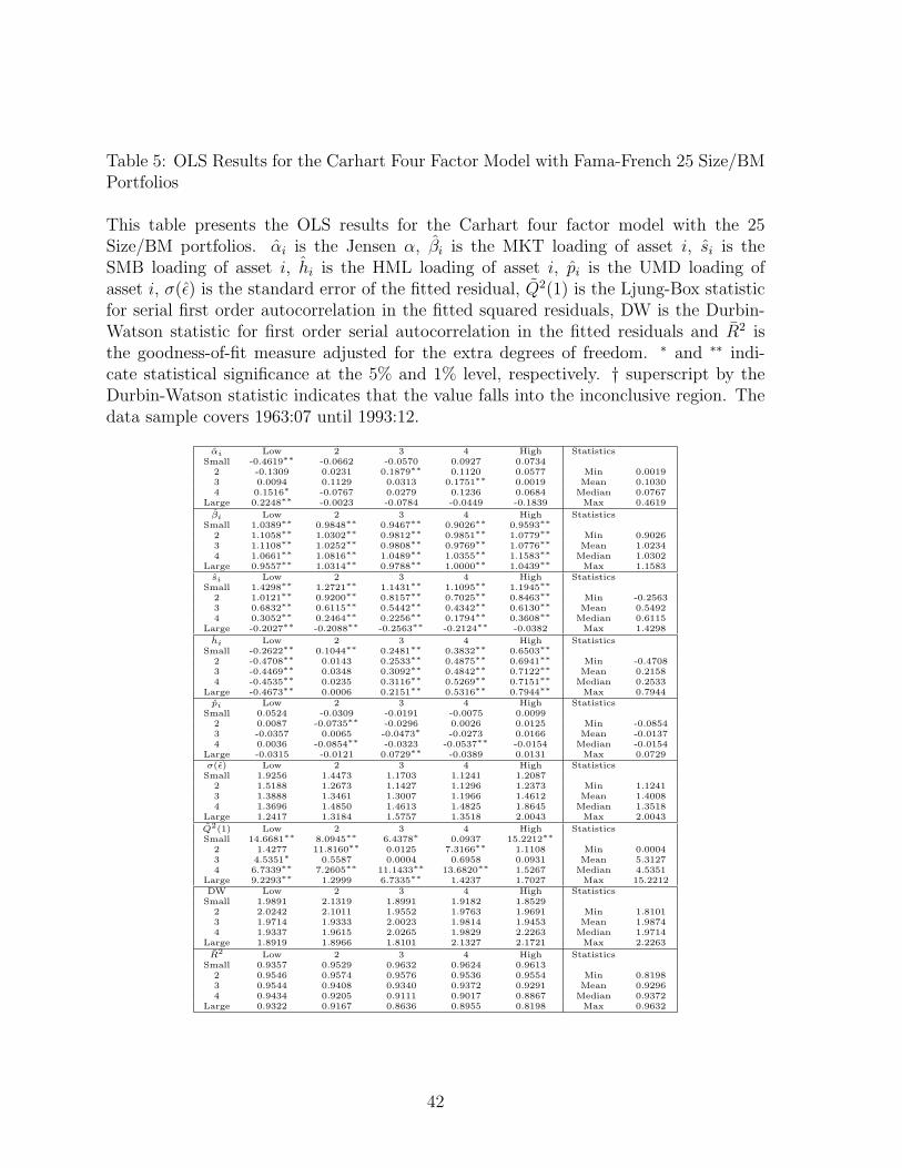
Table 5: OLS Results for the Carhart Four Factor Model with Fama-French 25 Size/BMPortfolios

This table presents the OLS results for the Carhart four factor model with the 25Size/BM portfolios. αi is the Jensen α, βi is the MKT loading of asset i, si is theSMB loading of asset i, hi is the HML loading of asset i, pi is the UMD loading ofasset i, σ(ε) is the standard error of the fitted residual, Q2(1) is the Ljung-Box statisticfor serial first order autocorrelation in the fitted squared residuals, DW is the Durbin-Watson statistic for first order serial autocorrelation in the fitted residuals and R2 isthe goodness-of-fit measure adjusted for the extra degrees of freedom. ∗ and ∗∗ indi-cate statistical significance at the 5% and 1% level, respectively. † superscript by theDurbin-Watson statistic indicates that the value falls into the inconclusive region. Thedata sample covers 1963:07 until 1993:12.

αi Low 2 3 4 High StatisticsSmall -0.4619∗∗ -0.0662 -0.0570 0.0927 0.0734

2 -0.1309 0.0231 0.1879∗∗ 0.1120 0.0577 Min 0.00193 0.0094 0.1129 0.0313 0.1751∗∗ 0.0019 Mean 0.10304 0.1516∗ -0.0767 0.0279 0.1236 0.0684 Median 0.0767

Large 0.2248∗∗ -0.0023 -0.0784 -0.0449 -0.1839 Max 0.4619


2 1.1058∗∗ 1.0302∗∗ 0.9812∗∗ 0.9851∗∗ 1.0779∗∗ Min 0.90263 1.1108∗∗ 1.0252∗∗ 0.9808∗∗ 0.9769∗∗ 1.0776∗∗ Mean 1.02344 1.0661∗∗ 1.0816∗∗ 1.0489∗∗ 1.0355∗∗ 1.1583∗∗ Median 1.0302

Large 0.9557∗∗ 1.0314∗∗ 0.9788∗∗ 1.0000∗∗ 1.0439∗∗ Max 1.1583si Low 2 3 4 High Statistics

Small 1.4298∗∗ 1.2721∗∗ 1.1431∗∗ 1.1095∗∗ 1.1945∗∗2 1.0121∗∗ 0.9200∗∗ 0.8157∗∗ 0.7025∗∗ 0.8463∗∗ Min -0.25633 0.6832∗∗ 0.6115∗∗ 0.5442∗∗ 0.4342∗∗ 0.6130∗∗ Mean 0.54924 0.3052∗∗ 0.2464∗∗ 0.2256∗∗ 0.1794∗∗ 0.3608∗∗ Median 0.6115

Large -0.2027∗∗ -0.2088∗∗ -0.2563∗∗ -0.2124∗∗ -0.0382 Max 1.4298

hi Low 2 3 4 High StatisticsSmall -0.2622∗∗ 0.1044∗∗ 0.2481∗∗ 0.3832∗∗ 0.6503∗∗

2 -0.4708∗∗ 0.0143 0.2533∗∗ 0.4875∗∗ 0.6941∗∗ Min -0.47083 -0.4469∗∗ 0.0348 0.3092∗∗ 0.4842∗∗ 0.7122∗∗ Mean 0.21584 -0.4535∗∗ 0.0235 0.3116∗∗ 0.5269∗∗ 0.7151∗∗ Median 0.2533

Large -0.4673∗∗ 0.0006 0.2151∗∗ 0.5316∗∗ 0.7944∗∗ Max 0.7944pi Low 2 3 4 High Statistics

Small 0.0524 -0.0309 -0.0191 -0.0075 0.00992 0.0087 -0.0735∗∗ -0.0296 0.0026 0.0125 Min -0.08543 -0.0357 0.0065 -0.0473∗ -0.0273 0.0166 Mean -0.01374 0.0036 -0.0854∗∗ -0.0323 -0.0537∗∗ -0.0154 Median -0.0154

Large -0.0315 -0.0121 0.0729∗∗ -0.0389 0.0131 Max 0.0729σ(ε) Low 2 3 4 High StatisticsSmall 1.9256 1.4473 1.1703 1.1241 1.2087

2 1.5188 1.2673 1.1427 1.1296 1.2373 Min 1.12413 1.3888 1.3461 1.3007 1.1966 1.4612 Mean 1.40084 1.3696 1.4850 1.4613 1.4825 1.8645 Median 1.3518

Large 1.2417 1.3184 1.5757 1.3518 2.0043 Max 2.0043

Q2(1) Low 2 3 4 High StatisticsSmall 14.6681∗∗ 8.0945∗∗ 6.4378∗ 0.0937 15.2212∗∗

2 1.4277 11.8160∗∗ 0.0125 7.3166∗∗ 1.1108 Min 0.00043 4.5351∗ 0.5587 0.0004 0.6958 0.0931 Mean 5.31274 6.7339∗∗ 7.2605∗∗ 11.1433∗∗ 13.6820∗∗ 1.5267 Median 4.5351

Large 9.2293∗∗ 1.2999 6.7335∗∗ 1.4237 1.7027 Max 15.2212DW Low 2 3 4 High Statistics


Large 1.8919 1.8966 1.8101 2.1327 2.1721 Max 2.2263

R2 Low 2 3 4 High StatisticsSmall 0.9357 0.9529 0.9632 0.9624 0.9613

2 0.9546 0.9574 0.9576 0.9536 0.9554 Min 0.81983 0.9544 0.9408 0.9340 0.9372 0.9291 Mean 0.92964 0.9434 0.9205 0.9111 0.9017 0.8867 Median 0.9372

Large 0.9322 0.9167 0.8636 0.8955 0.8198 Max 0.9632

42

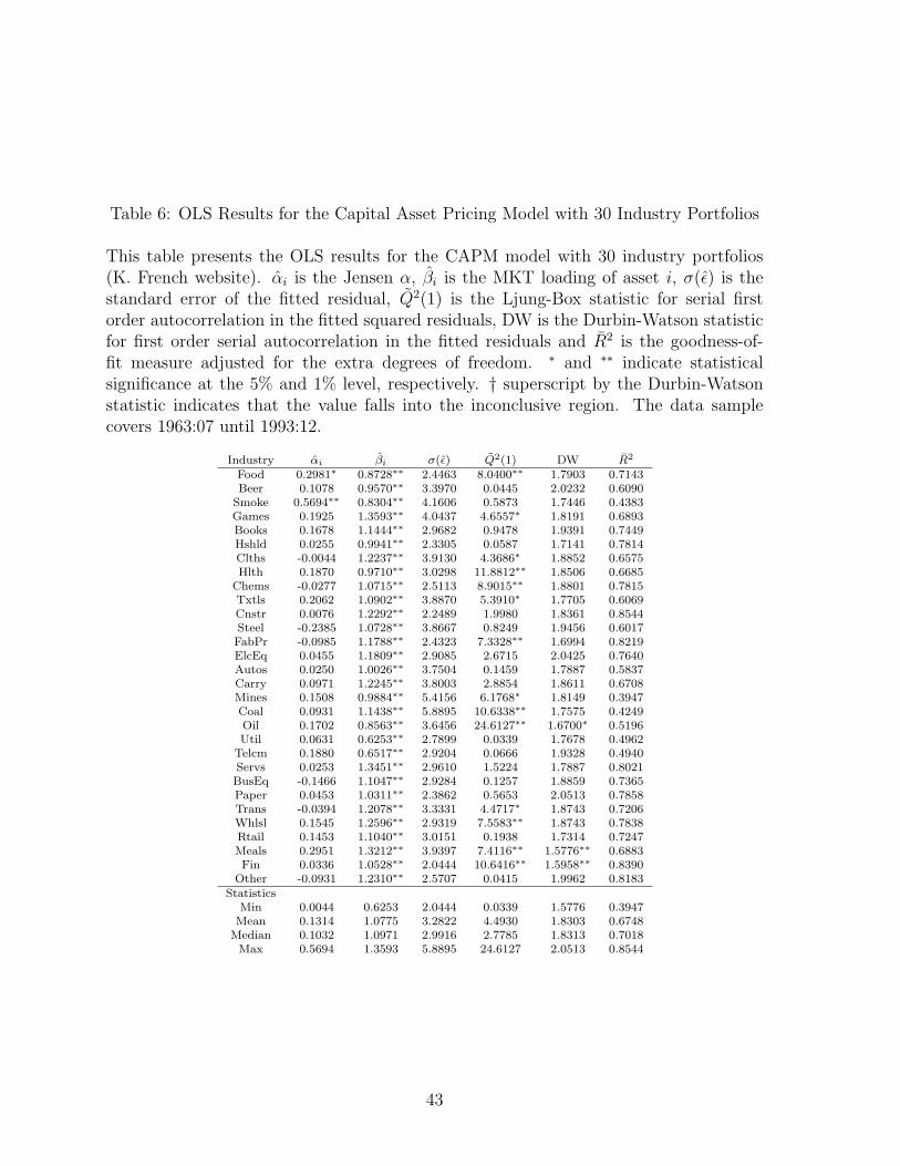
Table 6: OLS Results for the Capital Asset Pricing Model with 30 Industry Portfolios

This table presents the OLS results for the CAPM model with 30 industry portfolios(K. French website). αi is the Jensen α, βi is the MKT loading of asset i, σ(ε) is thestandard error of the fitted residual, Q2(1) is the Ljung-Box statistic for serial firstorder autocorrelation in the fitted squared residuals, DW is the Durbin-Watson statisticfor first order serial autocorrelation in the fitted residuals and R2 is the goodness-of-fit measure adjusted for the extra degrees of freedom. ∗ and ∗∗ indicate statisticalsignificance at the 5% and 1% level, respectively. † superscript by the Durbin-Watsonstatistic indicates that the value falls into the inconclusive region. The data samplecovers 1963:07 until 1993:12.

Industry αi βi σ(ε) Q2(1) DW R2

Food 0.2981∗ 0.8728∗∗ 2.4463 8.0400∗∗ 1.7903 0.7143Beer 0.1078 0.9570∗∗ 3.3970 0.0445 2.0232 0.6090

Smoke 0.5694∗∗ 0.8304∗∗ 4.1606 0.5873 1.7446 0.4383Games 0.1925 1.3593∗∗ 4.0437 4.6557∗ 1.8191 0.6893Books 0.1678 1.1444∗∗ 2.9682 0.9478 1.9391 0.7449Hshld 0.0255 0.9941∗∗ 2.3305 0.0587 1.7141 0.7814Clths -0.0044 1.2237∗∗ 3.9130 4.3686∗ 1.8852 0.6575Hlth 0.1870 0.9710∗∗ 3.0298 11.8812∗∗ 1.8506 0.6685

Chems -0.0277 1.0715∗∗ 2.5113 8.9015∗∗ 1.8801 0.7815Txtls 0.2062 1.0902∗∗ 3.8870 5.3910∗ 1.7705 0.6069Cnstr 0.0076 1.2292∗∗ 2.2489 1.9980 1.8361 0.8544Steel -0.2385 1.0728∗∗ 3.8667 0.8249 1.9456 0.6017FabPr -0.0985 1.1788∗∗ 2.4323 7.3328∗∗ 1.6994 0.8219ElcEq 0.0455 1.1809∗∗ 2.9085 2.6715 2.0425 0.7640Autos 0.0250 1.0026∗∗ 3.7504 0.1459 1.7887 0.5837Carry 0.0971 1.2245∗∗ 3.8003 2.8854 1.8611 0.6708Mines 0.1508 0.9884∗∗ 5.4156 6.1768∗ 1.8149 0.3947Coal 0.0931 1.1438∗∗ 5.8895 10.6338∗∗ 1.7575 0.4249Oil 0.1702 0.8563∗∗ 3.6456 24.6127∗∗ 1.6700∗ 0.5196Util 0.0631 0.6253∗∗ 2.7899 0.0339 1.7678 0.4962

Telcm 0.1880 0.6517∗∗ 2.9204 0.0666 1.9328 0.4940Servs 0.0253 1.3451∗∗ 2.9610 1.5224 1.7887 0.8021BusEq -0.1466 1.1047∗∗ 2.9284 0.1257 1.8859 0.7365Paper 0.0453 1.0311∗∗ 2.3862 0.5653 2.0513 0.7858Trans -0.0394 1.2078∗∗ 3.3331 4.4717∗ 1.8743 0.7206Whlsl 0.1545 1.2596∗∗ 2.9319 7.5583∗∗ 1.8743 0.7838Rtail 0.1453 1.1040∗∗ 3.0151 0.1938 1.7314 0.7247Meals 0.2951 1.3212∗∗ 3.9397 7.4116∗∗ 1.5776∗∗ 0.6883Fin 0.0336 1.0528∗∗ 2.0444 10.6416∗∗ 1.5958∗∗ 0.8390

Other -0.0931 1.2310∗∗ 2.5707 0.0415 1.9962 0.8183Statistics

Min 0.0044 0.6253 2.0444 0.0339 1.5776 0.3947Mean 0.1314 1.0775 3.2822 4.4930 1.8303 0.6748

Median 0.1032 1.0971 2.9916 2.7785 1.8313 0.7018Max 0.5694 1.3593 5.8895 24.6127 2.0513 0.8544

43

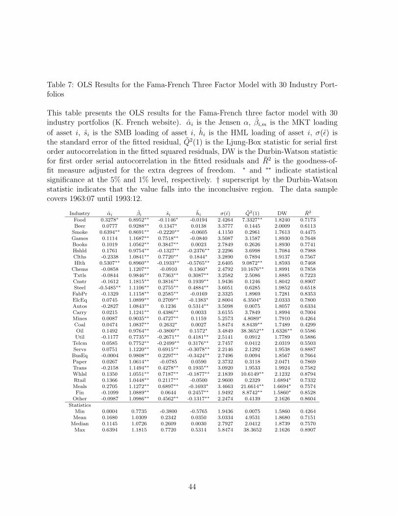
Table 7: OLS Results for the Fama-French Three Factor Model with 30 Industry Port-folios

This table presents the OLS results for the Fama-French three factor model with 30industry portfolios (K. French website). αi is the Jensen α, βi,m is the MKT loading

of asset i, si is the SMB loading of asset i, hi is the HML loading of asset i, σ(ε) isthe standard error of the fitted residual, Q2(1) is the Ljung-Box statistic for serial firstorder autocorrelation in the fitted squared residuals, DW is the Durbin-Watson statisticfor first order serial autocorrelation in the fitted residuals and R2 is the goodness-of-fit measure adjusted for the extra degrees of freedom. ∗ and ∗∗ indicate statisticalsignificance at the 5% and 1% level, respectively. † superscript by the Durbin-Watsonstatistic indicates that the value falls into the inconclusive region. The data samplecovers 1963:07 until 1993:12.

Industry αi βi si hi σ(ε) Q2(1) DW R2

Food 0.3278∗ 0.8952∗∗ -0.1146∗ -0.0194 2.4264 7.3327∗∗ 1.8240 0.7173Beer 0.0777 0.9288∗∗ 0.1347∗ 0.0138 3.3777 0.1445 2.0009 0.6113

Smoke 0.6394∗∗ 0.8691∗∗ -0.2220∗∗ -0.0605 4.1150 0.2961 1.7613 0.4475Games 0.1114 1.1687∗∗ 0.7518∗∗ -0.0840 3.5087 3.1587 1.8930 0.7648Books 0.1019 1.0562∗∗ 0.3847∗∗ 0.0023 2.7849 0.2626 1.8930 0.7741Hshld 0.1761 0.9754∗∗ -0.1327∗∗ -0.2376∗∗ 2.2296 3.6998 1.7084 0.7988Clths -0.2338 1.0841∗∗ 0.7720∗∗ 0.1844∗ 3.2890 0.7894 1.9137 0.7567Hlth 0.5307∗∗ 0.8960∗∗ -0.1933∗∗ -0.5765∗∗ 2.6405 9.0872∗∗ 1.8593 0.7468

Chems -0.0858 1.1207∗∗ -0.0910 0.1360∗ 2.4792 10.1676∗∗ 1.8991 0.7858Txtls -0.0844 0.9846∗∗ 0.7363∗∗ 0.3087∗∗ 3.2582 2.5086 1.8885 0.7223Cnstr -0.1612 1.1815∗∗ 0.3816∗∗ 0.1939∗∗ 1.9436 0.1246 1.8042 0.8907Steel -0.5485∗∗ 1.1106∗∗ 0.2755∗∗ 0.4884∗∗ 3.6051 0.6285 1.9852 0.6518FabPr -0.1329 1.1158∗∗ 0.2585∗∗ -0.0169 2.3325 1.8969 1.7281 0.8353ElcEq 0.0745 1.0899∗∗ 0.2709∗∗ -0.1383∗ 2.8004 6.3504∗ 2.0333 0.7800Autos -0.2827 1.0843∗∗ 0.1236 0.5314∗∗ 3.5098 0.0075 1.8057 0.6334Carry 0.0215 1.1241∗∗ 0.4386∗∗ 0.0033 3.6155 3.7849 1.8994 0.7004Mines 0.0087 0.9035∗∗ 0.4727∗∗ 0.1159 5.2573 4.8089∗ 1.7910 0.4264Coal 0.0474 1.0837∗∗ 0.2632∗ 0.0027 5.8474 8.8439∗∗ 1.7489 0.4299Oil 0.1492 0.9764∗∗ -0.3800∗∗ 0.1572∗ 3.4849 38.3652∗∗ 1.6326∗∗ 0.5586Util -0.1177 0.7735∗∗ -0.2671∗∗ 0.4181∗∗ 2.5141 0.0912 1.7789 0.5886

Telcm 0.0585 0.7752∗∗ -0.2499∗∗ 0.3176∗∗ 2.7457 0.0412 2.0319 0.5503Servs 0.0751 1.1220∗∗ 0.6915∗∗ -0.3078∗∗ 2.2146 2.1292 1.9538 0.8887BusEq -0.0004 0.9808∗∗ 0.2297∗∗ -0.3424∗∗ 2.7496 0.0094 1.8567 0.7664Paper 0.0267 1.0614∗∗ -0.0785 0.0590 2.3732 0.3118 2.0471 0.7869Trans -0.2158 1.1494∗∗ 0.4278∗∗ 0.1935∗∗ 3.0920 1.9533 1.9924 0.7582Whlsl 0.1350 1.0551∗∗ 0.7187∗∗ -0.1877∗∗ 2.1839 10.6149∗∗ 2.1232 0.8794Rtail 0.1366 1.0448∗∗ 0.2117∗∗ -0.0500 2.9600 0.2329 1.6894∗ 0.7332Meals 0.2705 1.1272∗∗ 0.6897∗∗ -0.1693∗ 3.4663 21.6614∗∗ 1.6694∗ 0.7574Fin -0.1099 1.0889∗∗ 0.0644 0.2457∗∗ 1.9492 8.8742∗∗ 1.5860∗ 0.8528

Other -0.0987 1.0986∗∗ 0.4562∗∗ -0.1317∗∗ 2.2474 0.4139 2.1626 0.8604Statistics

Min 0.0004 0.7735 -0.3800 -0.5765 1.9436 0.0075 1.5860 0.4264Mean 0.1680 1.0309 0.2342 0.0350 3.0334 4.9531 1.8680 0.7151

Median 0.1145 1.0726 0.2609 0.0030 2.7927 2.0412 1.8739 0.7570Max 0.6394 1.1815 0.7720 0.5314 5.8474 38.3652 2.1626 0.8907

44

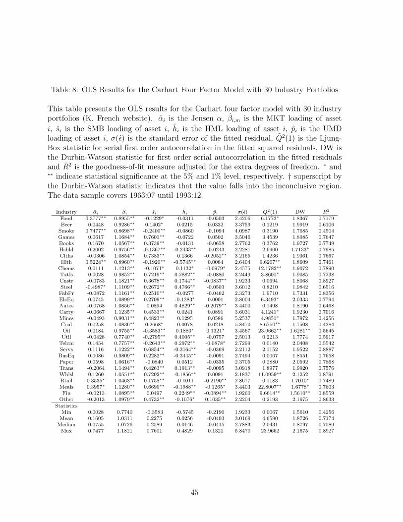
Table 8: OLS Results for the Carhart Four Factor Model with 30 Industry Portfolios

This table presents the OLS results for the Carhart four factor model with 30 industryportfolios (K. French website). αi is the Jensen α, βi,m is the MKT loading of asset

i, si is the SMB loading of asset i, hi is the HML loading of asset i, pi is the UMDloading of asset i, σ(ε) is the standard error of the fitted residual, Q2(1) is the Ljung-Box statistic for serial first order autocorrelation in the fitted squared residuals, DW isthe Durbin-Watson statistic for first order serial autocorrelation in the fitted residualsand R2 is the goodness-of-fit measure adjusted for the extra degrees of freedom. ∗ and∗∗ indicate statistical significance at the 5% and 1% level, respectively. † superscript bythe Durbin-Watson statistic indicates that the value falls into the inconclusive region.The data sample covers 1963:07 until 1993:12.

Industry αi βi si hi pi σ(ε) Q2(1) DW R2

Food 0.3777∗∗ 0.8955∗∗ -0.1229∗ -0.0311 -0.0503 2.4206 6.1773∗ 1.8367 0.7179Beer 0.0448 0.9286∗∗ 0.1402∗ 0.0215 0.0332 3.3759 0.1219 1.9919 0.6106

Smoke 0.7477∗∗ 0.8698∗∗ -0.2400∗∗ -0.0860 -0.1094 4.0987 0.3190 1.7685 0.4504Games 0.0617 1.1684∗∗ 0.7601∗∗ -0.0722 0.0502 3.5046 3.4539 1.8985 0.7647Books 0.1670 1.0567∗∗ 0.3739∗∗ -0.0131 -0.0658 2.7762 0.3762 1.9727 0.7749Hshld 0.2002 0.9756∗∗ -0.1367∗∗ -0.2433∗∗ -0.0243 2.2281 2.6900 1.7133∗ 0.7985Clths -0.0306 1.0854∗∗ 0.7383∗∗ 0.1366 -0.2052∗∗ 3.2165 1.4236 1.9361 0.7667Hlth 0.5224∗∗ 0.8960∗∗ -0.1920∗∗ -0.5745∗∗ 0.0084 2.6404 9.6207∗∗ 1.8609 0.7461

Chems 0.0111 1.1213∗∗ -0.1071∗ 0.1132∗ -0.0979∗ 2.4575 12.1782∗∗ 1.9072 0.7890Txtls 0.0028 0.9852∗∗ 0.7219∗∗ 0.2882∗∗ -0.0880 3.2449 3.8601∗ 1.9085 0.7238Cnstr -0.0783 1.1821∗∗ 0.3678∗∗ 0.1744∗∗ -0.0837∗∗ 1.9233 0.0694 1.8068 0.8927Steel -0.4987∗ 1.1109∗∗ 0.2672∗∗ 0.4766∗∗ -0.0503 3.6012 0.8210 1.9842 0.6516FabPr -0.0872 1.1161∗∗ 0.2510∗∗ -0.0277 -0.0462 2.3273 1.9710 1.7331 0.8356ElcEq 0.0745 1.0899∗∗ 0.2709∗∗ -0.1383∗ 0.0001 2.8004 6.3493∗ 2.0333 0.7794Autos -0.0768 1.0856∗∗ 0.0894 0.4829∗∗ -0.2079∗∗ 3.4400 0.1498 1.8190 0.6468Carry -0.0667 1.1235∗∗ 0.4533∗∗ 0.0241 0.0891 3.6031 4.1241∗ 1.9230 0.7016Mines -0.0493 0.9031∗∗ 0.4823∗∗ 0.1295 0.0586 5.2537 4.9851∗ 1.7972 0.4256Coal 0.0258 1.0836∗∗ 0.2668∗ 0.0078 0.0218 5.8470 8.6750∗∗ 1.7508 0.4284Oil 0.0184 0.9755∗∗ -0.3583∗∗ 0.1880∗ 0.1321∗ 3.4567 23.9662∗∗ 1.6281∗∗ 0.5645Util -0.0428 0.7740∗∗ -0.2795∗∗ 0.4005∗∗ -0.0757 2.5013 0.2213 1.7774 0.5917

Telcm 0.1454 0.7757∗∗ -0.2643∗∗ 0.2972∗∗ -0.0878∗ 2.7299 0.0140 2.0408 0.5542Servs 0.1116 1.1222∗∗ 0.6854∗∗ -0.3164∗∗ -0.0369 2.2112 2.1152 1.9522 0.8887BusEq 0.0086 0.9809∗∗ 0.2282∗∗ -0.3445∗∗ -0.0091 2.7494 0.0067 1.8551 0.7658Paper 0.0598 1.0616∗∗ -0.0840 0.0512 -0.0335 2.3705 0.2880 2.0592 0.7868Trans -0.2064 1.1494∗∗ 0.4263∗∗ 0.1913∗∗ -0.0095 3.0918 1.8977 1.9920 0.7576Whlsl 0.1260 1.0551∗∗ 0.7202∗∗ -0.1856∗∗ 0.0091 2.1837 11.0959∗∗ 2.1252 0.8791Rtail 0.3535∗ 1.0463∗∗ 0.1758∗∗ -0.1011 -0.2190∗∗ 2.8677 0.1183 1.7010∗ 0.7489Meals 0.3957∗ 1.1280∗∗ 0.6690∗∗ -0.1988∗∗ -0.1265∗ 3.4403 22.8007∗∗ 1.6778∗ 0.7603Fin -0.0213 1.0895∗∗ 0.0497 0.2249*∗ -0.0894∗∗ 1.9260 9.6614∗∗ 1.5610∗∗ 0.8559

Other -0.2013 1.0979∗∗ 0.4732∗∗ -0.1076∗ 0.1035∗∗ 2.2204 0.2193 2.1675 0.8633Statistics

Min 0.0028 0.7740 -0.3583 -0.5745 -0.2190 1.9233 0.0067 1.5610 0.4256Mean 0.1605 1.0311 0.2275 0.0256 -0.0403 3.0169 4.6590 1.8726 0.7174

Median 0.0755 1.0726 0.2589 0.0146 -0.0415 2.7883 2.0431 1.8797 0.7589Max 0.7477 1.1821 0.7601 0.4829 0.1321 5.8470 23.9662 2.1675 0.8927

45

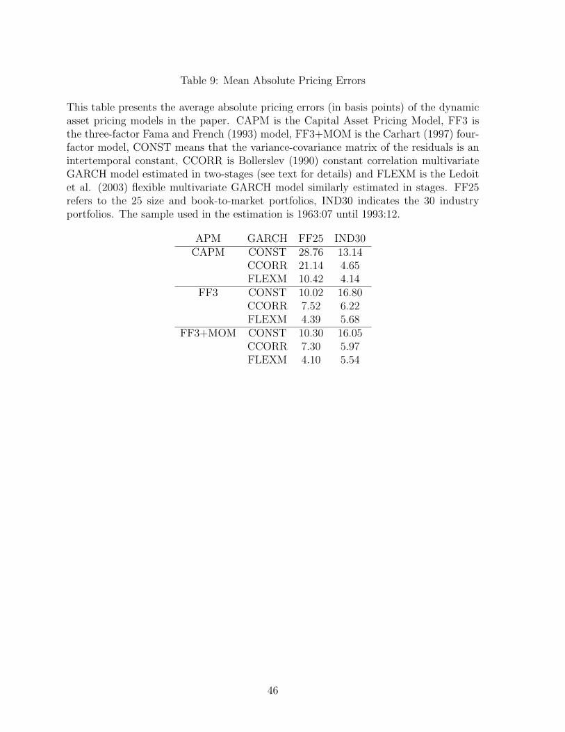
Table 9: Mean Absolute Pricing Errors

This table presents the average absolute pricing errors (in basis points) of the dynamicasset pricing models in the paper. CAPM is the Capital Asset Pricing Model, FF3 isthe three-factor Fama and French (1993) model, FF3+MOM is the Carhart (1997) four-factor model, CONST means that the variance-covariance matrix of the residuals is anintertemporal constant, CCORR is Bollerslev (1990) constant correlation multivariateGARCH model estimated in two-stages (see text for details) and FLEXM is the Ledoitet al. (2003) flexible multivariate GARCH model similarly estimated in stages. FF25refers to the 25 size and book-to-market portfolios, IND30 indicates the 30 industryportfolios. The sample used in the estimation is 1963:07 until 1993:12.

APM GARCH FF25 IND30CAPM CONST 28.76 13.14

CCORR 21.14 4.65FLEXM 10.42 4.14

FF3 CONST 10.02 16.80CCORR 7.52 6.22FLEXM 4.39 5.68

FF3+MOM CONST 10.30 16.05CCORR 7.30 5.97FLEXM 4.10 5.54

46

Table 10: Hypotheses Tests with Fama-French 25 Size/BM Portfolios

This table presents the hypotheses test results for three factor models using the 25 sizeand book-to-market portfolios as test assets. CAPM is the Capital Asset Pricing Model,FF3 is the three-factor Fama and French (1993) model, FF3+MOM is the Carhart(1997) four-factor model, CONST means that the variance-covariance matrix of theresiduals is an intertemporal constant, CCORR is Bollerslev (1990) constant correlationmultivariate GARCH model estimated in two-stages (see text for details) and FLEXMis the Ledoit et al. (2003) flexible multivariate GARCH model similarly estimated instages. The Wald statistic used to perform the tests has a χ2 asymptotic distributionwith the indicated number of degrees of freedom. The sample used in the estimation is1963:07 until 1993:12.

APM GARCH H0 df Wald p-value

CAPM CONST α = 0 25 144.84 0.0000CCORR α = 0 25 588.39 0.0000FLEXM α = 0 25 556.88 0.0000

FF3 CONST α = 0 25 65.75 0.0000CCORR α = 0 25 71.77 0.0000FLEXM α = 0 25 96.11 0.0000CONST s = h = 0 50 25803.13 0.0000CCORR s = h = 0 50 96667.91 0.0000FLEXM s = h = 0 50 93892.49 0.0000

FF3+MOM CONST α = 0 25 68.93 0.0000CCORR α = 0 25 70.88 0.0000FLEXM α = 0 25 64.50 0.0000CONST s = h = 0 50 25103.04 0.0000CCORR s = h = 0 50 97105.58 0.0000FLEXM s = h = 0 50 93809.10 0.0000CONST p = 0 25 70.90 0.0000CCORR p = 0 25 5703.53 0.0000FLEXM p = 0 25 4953.86 0.0000CONST s = h = p = 0 75 11606.75 0.0000CCORR s = h = p = 0 75 102209.11 0.0000FLEXM s = h = p = 0 75 98852.96 0.0000

47

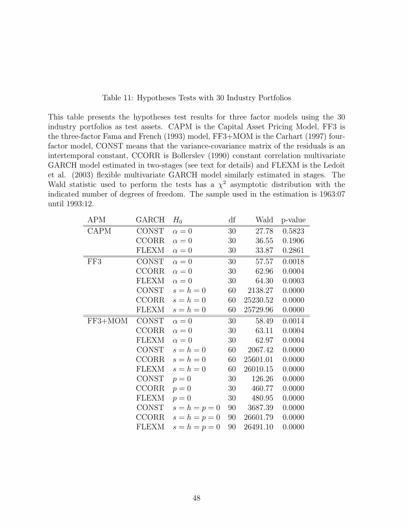
Table 11: Hypotheses Tests with 30 Industry Portfolios

This table presents the hypotheses test results for three factor models using the 30industry portfolios as test assets. CAPM is the Capital Asset Pricing Model, FF3 isthe three-factor Fama and French (1993) model, FF3+MOM is the Carhart (1997) four-factor model, CONST means that the variance-covariance matrix of the residuals is anintertemporal constant, CCORR is Bollerslev (1990) constant correlation multivariateGARCH model estimated in two-stages (see text for details) and FLEXM is the Ledoitet al. (2003) flexible multivariate GARCH model similarly estimated in stages. TheWald statistic used to perform the tests has a χ2 asymptotic distribution with theindicated number of degrees of freedom. The sample used in the estimation is 1963:07until 1993:12.

APM GARCH H0 df Wald p-value

CAPM CONST α = 0 30 27.78 0.5823CCORR α = 0 30 36.55 0.1906FLEXM α = 0 30 33.87 0.2861

FF3 CONST α = 0 30 57.57 0.0018CCORR α = 0 30 62.96 0.0004FLEXM α = 0 30 64.30 0.0003CONST s = h = 0 60 2138.27 0.0000CCORR s = h = 0 60 25230.52 0.0000FLEXM s = h = 0 60 25729.96 0.0000

FF3+MOM CONST α = 0 30 58.49 0.0014CCORR α = 0 30 63.11 0.0004FLEXM α = 0 30 62.97 0.0004CONST s = h = 0 60 2067.42 0.0000CCORR s = h = 0 60 25601.01 0.0000FLEXM s = h = 0 60 26010.15 0.0000CONST p = 0 30 126.26 0.0000CCORR p = 0 30 460.77 0.0000FLEXM p = 0 30 480.95 0.0000CONST s = h = p = 0 90 3687.39 0.0000CCORR s = h = p = 0 90 26601.79 0.0000FLEXM s = h = p = 0 90 26491.10 0.0000

48

Table 12: Instrumental Variable Regressions for OLS Residuals from of the 25 Size/BMPortfolios

This table presents the results from the regression of the OLS residuals of the 25 Fama-French portfolios on a set of instrumental variables. The instrumental variables includea constant, the lagged long-term government bond return SBBI (LTGB), the laggeddividend yield on the NYSE/AMEX value-weighted index from CRSP (D/P), the laggeddefault spread defined as Moody’s Baa corporate bond yield minus the Aaa yield (DEF)and the lagged term spread defined as the 10 year Treasury bond yield minus the 1month Treasury bill yield (TERM). P-value is the probability value of the F test of thenull hypothesis that all the coefficients in the linear regression are equal to zero. Themonthly returns cover the period 1963:07 to 1993:12. Stars indicate significance at the5% level.

Residual Const. LTGB D/P DEF TERM R2 p-val.ε11 0.6092 -0.1322∗ -0.0445 -0.2853 -0.1953∗ 0.0565 0.0003∗

ε12 0.4210 -0.0820∗ -0.1545 0.2191 -0.1244 0.0343 0.0131∗

ε13 -0.0285 -0.0543∗ -0.1067 0.4373∗ -0.0721 0.0369 0.0086∗

ε14 0.7596∗ -0.0175 -0.3185∗ 0.4667∗ -0.1311∗ 0.0469 0.0016∗

ε15 0.9623∗ -0.0507∗ -0.3565∗ 0.3739∗ -0.0631 0.0429 0.0032∗

ε21 -0.1532 -0.0787∗ 0.0907 -0.1399 -0.0393 0.0267 0.0438∗

ε22 -0.7087∗ -0.0258 0.1141 0.2576 0.0124 0.0233 0.0734ε23 0.4566 -0.0028 -0.2185∗ 0.2985 0.0502 0.0191 0.1377ε24 -0.5028 0.0205 0.1091 0.0531 0.0608 0.0125 0.3368ε25 0.2008 0.0006 -0.0173 -0.1271 0.0020 0.0032 0.8865ε31 -0.2643 -0.0339 0.0604 0.0571 -0.0305 0.0079 0.5801ε32 -0.3345 0.0559∗ 0.0248 0.2025 0.0275 0.0234 0.0723ε33 -0.0889 0.0698∗ 0.0156 -0.0095 0.0557 0.0252 0.0556ε34 0.4673 0.0325 -0.1311 0.0356 -0.0354 0.0135 0.2938ε35 -0.1808 -0.0279 0.1319 -0.2737 -0.0151 0.0095 0.4854ε41 -0.1925 -0.0350 0.0537 0.0001 -0.0058 0.0066 0.6626ε42 -0.6377 0.0525 0.1573 0.0067 0.0660 0.0174 0.1748ε43 -0.0741 0.0227 0.0226 0.0102 -0.0371 0.0040 0.8368ε44 0.4081 0.0164 -0.0472 -0.1619 -0.0940 0.0097 0.4736ε45 0.1893 -0.0650 -0.0491 0.0445 -0.0787 0.0116 0.3777ε51 0.8039∗ -0.0183 -0.3164∗ 0.3745∗ -0.0538 0.0252 0.0551ε52 -0.6411 -0.0012 0.1263 0.1133 0.0790 0.0131 0.3118ε53 -0.6204 0.0397 0.3521∗ -0.6863∗ 0.0870 0.0310 0.0225∗

ε54 -0.0992 -0.0414 0.0860 -0.1070 -0.1607∗ 0.0295 0.0283∗

ε55 0.9473 -0.0624 -0.4159∗ 0.5716∗ -0.0274 0.0223 0.0861

49

Table 13: Instrumental Variable Regressions of Squared OLS Residuals of the 25Size/BM Portfolios

This table presents the results from the regression of the squared OLS residuals of the 25Fama-French portfolios on a set of instrumental variables. The instrumental variablesinclude a constant, the lagged long-term government bond return SBBI (LTGB), thelagged dividend yield on the NYSE/AMEX value-weighted index from CRSP (D/P),the lagged default spread defined as Moody’s Baa corporate bond yield minus the Aaayield (DEF) and the lagged term spread defined as the 10 year Treasury bond yield minusthe 1 month Treasury bill yield (TERM). P-value is the probability value of the F testof the null hypothesis that all the coefficients in the linear regression are equal to zero.The monthly returns cover the period 1963:07 to 1993:12. Stars indicate significance atthe 5% level.

Sq. Res. Const. LTGB D/P DEF TERM R2 p-val.ε211 3.3397∗ -0.0642 -0.6832 2.6302∗ 0.1229 0.0261 0.0480∗

ε212 3.4867∗ 0.0643 -0.4597 0.4087 -0.2085 0.0198 0.1244

ε213 2.7192∗ -0.0124 -0.4059∗ 0.2293 -0.1441 0.0180 0.1597

ε214 1.4022∗ 0.0262 -0.0150 -0.0750 -0.0112 0.0023 0.9342

ε215 1.6785∗ 0.0263 -0.0374 -0.0456 -0.0556 0.0023 0.9342

ε221 4.8297∗ -0.0208 -0.4094 -0.7194 -0.3613∗ 0.0286 0.0327∗

ε222 0.7369 -0.0349 0.3471 -0.2841 -0.0844 0.0087 0.5338

ε223 1.4025∗ 0.0016 -0.0033 -0.0313 -0.0714 0.0016 0.9639

ε224 0.6325 -0.0262 0.2132 -0.1178 -0.0343 0.0087 0.5339

ε225 2.4181∗ 0.0394 -0.4351∗ 0.6780 -0.0213 0.0162 0.2055

ε231 3.9195∗ -0.0248 -0.6541∗ 0.3885 0.0455 0.0235 0.0717

ε232 2.2672∗ -0.0845 0.0462 -0.4678 -0.1853 0.0202 0.1166

ε233 2.6669∗ -0.1115∗ -0.3089 0.3569 -0.2964∗ 0.0262 0.0478∗

ε234 0.5961 -0.1270∗ 0.2168 0.1211 -0.1355 0.0402 0.0051∗

ε235 1.4964 -0.0442 0.0723 0.2875 0.0959 0.0046 0.7976

ε241 3.7230∗ -0.0884 -0.5455∗ 0.1547 0.0235 0.0263 0.0469∗

ε242 3.0834∗ 0.0172 -0.0771 -0.3572 -0.2094 0.0061 0.6990

ε243 1.5814 -0.0767 0.0086 0.7292 -0.4121∗ 0.0273 0.0401∗

ε244 0.9110 -0.1848∗ 0.2929 0.2365 -0.0222 0.0213 0.0996

ε245 5.6233∗ -0.0115 -1.0060∗ 1.3300 0.2250 0.0197 0.1261

ε251 0.2707 -0.1439∗ 0.2088 0.4819 -0.0115 0.0417 0.0039∗

ε252 0.6436 -0.0485 -0.0804 1.1490∗ 0.2368∗ 0.0550 0.0004∗

ε253 0.1294 -0.2396∗ 0.0183 1.8587∗ 0.5508∗ 0.0397 0.0055∗

ε254 1.8851∗ -0.1003 -0.2585 0.9022∗ -0.0893 0.0211 0.1024

ε255 3.8050 -0.0097 -0.0742 0.4706 -0.0506 0.0008 0.9913

50

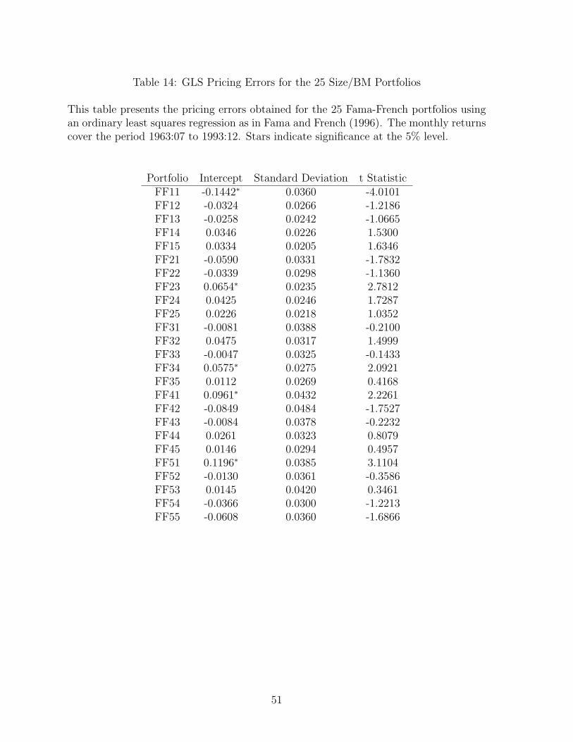
Table 14: GLS Pricing Errors for the 25 Size/BM Portfolios

This table presents the pricing errors obtained for the 25 Fama-French portfolios usingan ordinary least squares regression as in Fama and French (1996). The monthly returnscover the period 1963:07 to 1993:12. Stars indicate significance at the 5% level.

Portfolio Intercept Standard Deviation t StatisticFF11 -0.1442∗ 0.0360 -4.0101FF12 -0.0324 0.0266 -1.2186FF13 -0.0258 0.0242 -1.0665FF14 0.0346 0.0226 1.5300FF15 0.0334 0.0205 1.6346FF21 -0.0590 0.0331 -1.7832FF22 -0.0339 0.0298 -1.1360FF23 0.0654∗ 0.0235 2.7812FF24 0.0425 0.0246 1.7287FF25 0.0226 0.0218 1.0352FF31 -0.0081 0.0388 -0.2100FF32 0.0475 0.0317 1.4999FF33 -0.0047 0.0325 -0.1433FF34 0.0575∗ 0.0275 2.0921FF35 0.0112 0.0269 0.4168FF41 0.0961∗ 0.0432 2.2261FF42 -0.0849 0.0484 -1.7527FF43 -0.0084 0.0378 -0.2232FF44 0.0261 0.0323 0.8079FF45 0.0146 0.0294 0.4957FF51 0.1196∗ 0.0385 3.1104FF52 -0.0130 0.0361 -0.3586FF53 0.0145 0.0420 0.3461FF54 -0.0366 0.0300 -1.2213FF55 -0.0608 0.0360 -1.6866

51

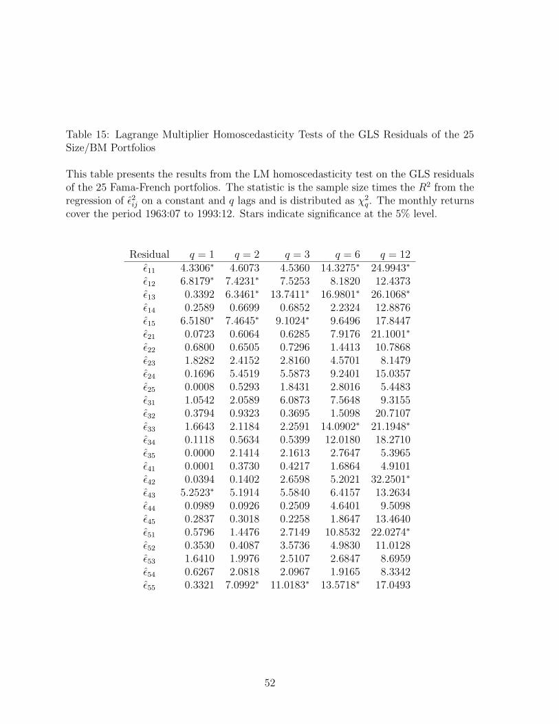
Table 15: Lagrange Multiplier Homoscedasticity Tests of the GLS Residuals of the 25Size/BM Portfolios

This table presents the results from the LM homoscedasticity test on the GLS residualsof the 25 Fama-French portfolios. The statistic is the sample size times the R2 from theregression of ε2

ij on a constant and q lags and is distributed as χ2q. The monthly returns

cover the period 1963:07 to 1993:12. Stars indicate significance at the 5% level.

Residual q = 1 q = 2 q = 3 q = 6 q = 12ε11 4.3306∗ 4.6073 4.5360 14.3275∗ 24.9943∗

ε12 6.8179∗ 7.4231∗ 7.5253 8.1820 12.4373ε13 0.3392 6.3461∗ 13.7411∗ 16.9801∗ 26.1068∗

ε14 0.2589 0.6699 0.6852 2.2324 12.8876ε15 6.5180∗ 7.4645∗ 9.1024∗ 9.6496 17.8447ε21 0.0723 0.6064 0.6285 7.9176 21.1001∗

ε22 0.6800 0.6505 0.7296 1.4413 10.7868ε23 1.8282 2.4152 2.8160 4.5701 8.1479ε24 0.1696 5.4519 5.5873 9.2401 15.0357ε25 0.0008 0.5293 1.8431 2.8016 5.4483ε31 1.0542 2.0589 6.0873 7.5648 9.3155ε32 0.3794 0.9323 0.3695 1.5098 20.7107ε33 1.6643 2.1184 2.2591 14.0902∗ 21.1948∗

ε34 0.1118 0.5634 0.5399 12.0180 18.2710ε35 0.0000 2.1414 2.1613 2.7647 5.3965ε41 0.0001 0.3730 0.4217 1.6864 4.9101ε42 0.0394 0.1402 2.6598 5.2021 32.2501∗

ε43 5.2523∗ 5.1914 5.5840 6.4157 13.2634ε44 0.0989 0.0926 0.2509 4.6401 9.5098ε45 0.2837 0.3018 0.2258 1.8647 13.4640ε51 0.5796 1.4476 2.7149 10.8532 22.0274∗

ε52 0.3530 0.4087 3.5736 4.9830 11.0128ε53 1.6410 1.9976 2.5107 2.6847 8.6959ε54 0.6267 2.0818 2.0967 1.9165 8.3342ε55 0.3321 7.0992∗ 11.0183∗ 13.5718∗ 17.0493

52

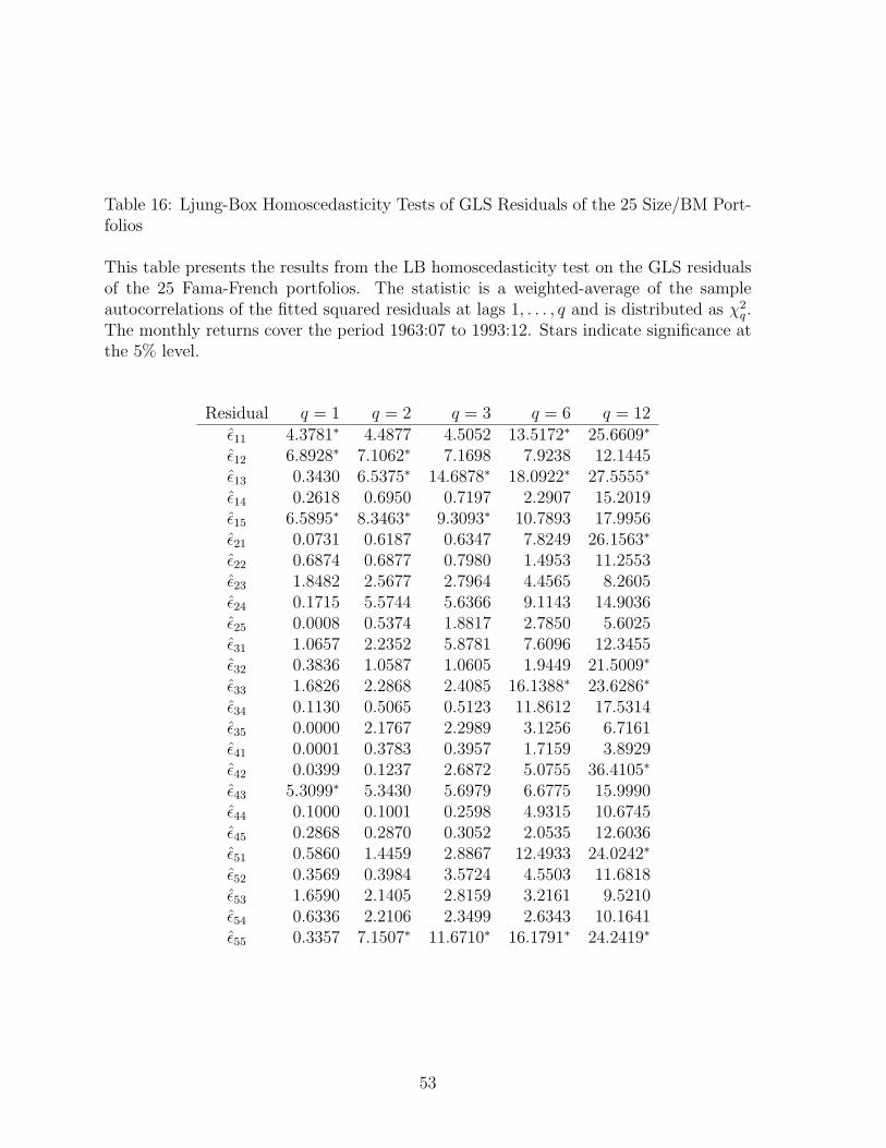
Table 16: Ljung-Box Homoscedasticity Tests of GLS Residuals of the 25 Size/BM Port-folios

This table presents the results from the LB homoscedasticity test on the GLS residualsof the 25 Fama-French portfolios. The statistic is a weighted-average of the sampleautocorrelations of the fitted squared residuals at lags 1, . . . , q and is distributed as χ2

q.The monthly returns cover the period 1963:07 to 1993:12. Stars indicate significance atthe 5% level.

Residual q = 1 q = 2 q = 3 q = 6 q = 12ε11 4.3781∗ 4.4877 4.5052 13.5172∗ 25.6609∗

ε12 6.8928∗ 7.1062∗ 7.1698 7.9238 12.1445ε13 0.3430 6.5375∗ 14.6878∗ 18.0922∗ 27.5555∗

ε14 0.2618 0.6950 0.7197 2.2907 15.2019ε15 6.5895∗ 8.3463∗ 9.3093∗ 10.7893 17.9956ε21 0.0731 0.6187 0.6347 7.8249 26.1563∗

ε22 0.6874 0.6877 0.7980 1.4953 11.2553ε23 1.8482 2.5677 2.7964 4.4565 8.2605ε24 0.1715 5.5744 5.6366 9.1143 14.9036ε25 0.0008 0.5374 1.8817 2.7850 5.6025ε31 1.0657 2.2352 5.8781 7.6096 12.3455ε32 0.3836 1.0587 1.0605 1.9449 21.5009∗

ε33 1.6826 2.2868 2.4085 16.1388∗ 23.6286∗

ε34 0.1130 0.5065 0.5123 11.8612 17.5314ε35 0.0000 2.1767 2.2989 3.1256 6.7161ε41 0.0001 0.3783 0.3957 1.7159 3.8929ε42 0.0399 0.1237 2.6872 5.0755 36.4105∗

ε43 5.3099∗ 5.3430 5.6979 6.6775 15.9990ε44 0.1000 0.1001 0.2598 4.9315 10.6745ε45 0.2868 0.2870 0.3052 2.0535 12.6036ε51 0.5860 1.4459 2.8867 12.4933 24.0242∗

ε52 0.3569 0.3984 3.5724 4.5503 11.6818ε53 1.6590 2.1405 2.8159 3.2161 9.5210ε54 0.6336 2.2106 2.3499 2.6343 10.1641ε55 0.3357 7.1507∗ 11.6710∗ 16.1791∗ 24.2419∗

53

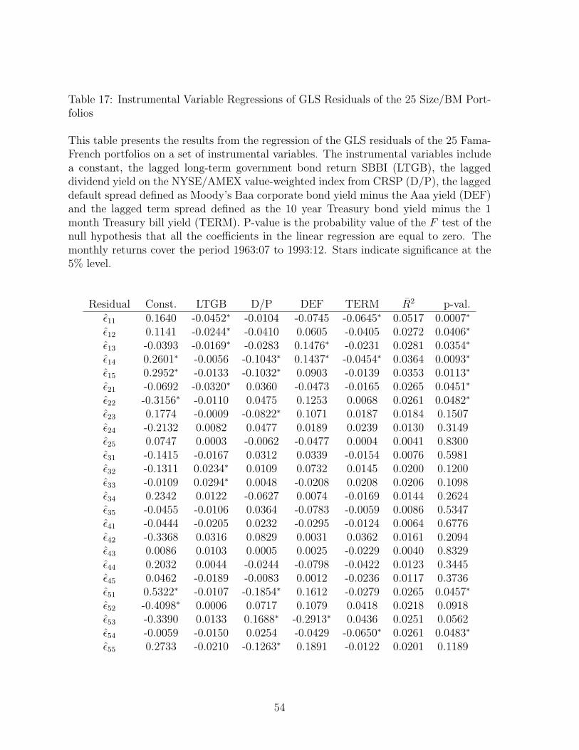
Table 17: Instrumental Variable Regressions of GLS Residuals of the 25 Size/BM Port-folios

This table presents the results from the regression of the GLS residuals of the 25 Fama-French portfolios on a set of instrumental variables. The instrumental variables includea constant, the lagged long-term government bond return SBBI (LTGB), the laggeddividend yield on the NYSE/AMEX value-weighted index from CRSP (D/P), the laggeddefault spread defined as Moody’s Baa corporate bond yield minus the Aaa yield (DEF)and the lagged term spread defined as the 10 year Treasury bond yield minus the 1month Treasury bill yield (TERM). P-value is the probability value of the F test of thenull hypothesis that all the coefficients in the linear regression are equal to zero. Themonthly returns cover the period 1963:07 to 1993:12. Stars indicate significance at the5% level.

Residual Const. LTGB D/P DEF TERM R2 p-val.ε11 0.1640 -0.0452∗ -0.0104 -0.0745 -0.0645∗ 0.0517 0.0007∗

ε12 0.1141 -0.0244∗ -0.0410 0.0605 -0.0405 0.0272 0.0406∗

ε13 -0.0393 -0.0169∗ -0.0283 0.1476∗ -0.0231 0.0281 0.0354∗

ε14 0.2601∗ -0.0056 -0.1043∗ 0.1437∗ -0.0454∗ 0.0364 0.0093∗

ε15 0.2952∗ -0.0133 -0.1032∗ 0.0903 -0.0139 0.0353 0.0113∗

ε21 -0.0692 -0.0320∗ 0.0360 -0.0473 -0.0165 0.0265 0.0451∗

ε22 -0.3156∗ -0.0110 0.0475 0.1253 0.0068 0.0261 0.0482∗

ε23 0.1774 -0.0009 -0.0822∗ 0.1071 0.0187 0.0184 0.1507ε24 -0.2132 0.0082 0.0477 0.0189 0.0239 0.0130 0.3149ε25 0.0747 0.0003 -0.0062 -0.0477 0.0004 0.0041 0.8300ε31 -0.1415 -0.0167 0.0312 0.0339 -0.0154 0.0076 0.5981ε32 -0.1311 0.0234∗ 0.0109 0.0732 0.0145 0.0200 0.1200ε33 -0.0109 0.0294∗ 0.0048 -0.0208 0.0208 0.0206 0.1098ε34 0.2342 0.0122 -0.0627 0.0074 -0.0169 0.0144 0.2624ε35 -0.0455 -0.0106 0.0364 -0.0783 -0.0059 0.0086 0.5347ε41 -0.0444 -0.0205 0.0232 -0.0295 -0.0124 0.0064 0.6776ε42 -0.3368 0.0316 0.0829 0.0031 0.0362 0.0161 0.2094ε43 0.0086 0.0103 0.0005 0.0025 -0.0229 0.0040 0.8329ε44 0.2032 0.0044 -0.0244 -0.0798 -0.0422 0.0123 0.3445ε45 0.0462 -0.0189 -0.0083 0.0012 -0.0236 0.0117 0.3736ε51 0.5322∗ -0.0107 -0.1854∗ 0.1612 -0.0279 0.0265 0.0457∗

ε52 -0.4098∗ 0.0006 0.0717 0.1079 0.0418 0.0218 0.0918ε53 -0.3390 0.0133 0.1688∗ -0.2913∗ 0.0436 0.0251 0.0562ε54 -0.0059 -0.0150 0.0254 -0.0429 -0.0650∗ 0.0261 0.0483∗

ε55 0.2733 -0.0210 -0.1263∗ 0.1891 -0.0122 0.0201 0.1189

54

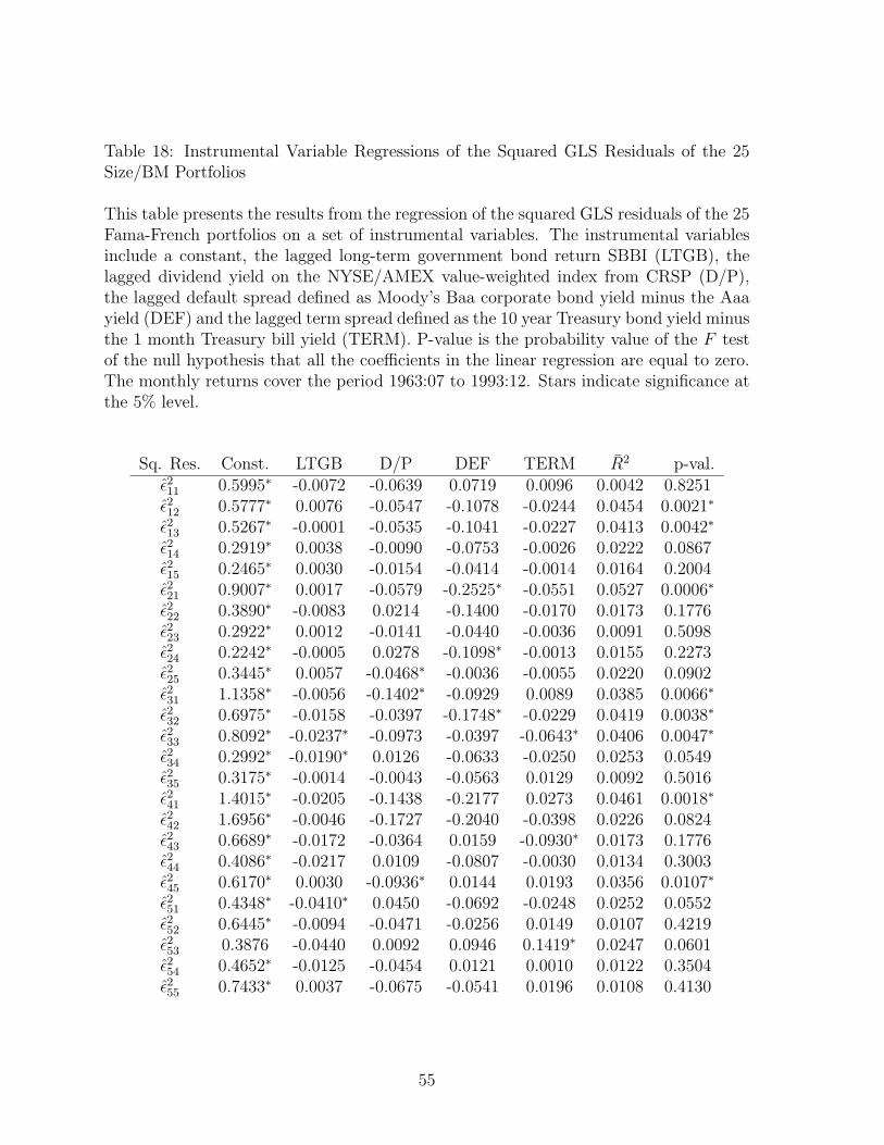
Table 18: Instrumental Variable Regressions of the Squared GLS Residuals of the 25Size/BM Portfolios

This table presents the results from the regression of the squared GLS residuals of the 25Fama-French portfolios on a set of instrumental variables. The instrumental variablesinclude a constant, the lagged long-term government bond return SBBI (LTGB), thelagged dividend yield on the NYSE/AMEX value-weighted index from CRSP (D/P),the lagged default spread defined as Moody’s Baa corporate bond yield minus the Aaayield (DEF) and the lagged term spread defined as the 10 year Treasury bond yield minusthe 1 month Treasury bill yield (TERM). P-value is the probability value of the F testof the null hypothesis that all the coefficients in the linear regression are equal to zero.The monthly returns cover the period 1963:07 to 1993:12. Stars indicate significance atthe 5% level.

Sq. Res. Const. LTGB D/P DEF TERM R2 p-val.ε211 0.5995∗ -0.0072 -0.0639 0.0719 0.0096 0.0042 0.8251

ε212 0.5777∗ 0.0076 -0.0547 -0.1078 -0.0244 0.0454 0.0021∗

ε213 0.5267∗ -0.0001 -0.0535 -0.1041 -0.0227 0.0413 0.0042∗

ε214 0.2919∗ 0.0038 -0.0090 -0.0753 -0.0026 0.0222 0.0867

ε215 0.2465∗ 0.0030 -0.0154 -0.0414 -0.0014 0.0164 0.2004

ε221 0.9007∗ 0.0017 -0.0579 -0.2525∗ -0.0551 0.0527 0.0006∗

ε222 0.3890∗ -0.0083 0.0214 -0.1400 -0.0170 0.0173 0.1776

ε223 0.2922∗ 0.0012 -0.0141 -0.0440 -0.0036 0.0091 0.5098

ε224 0.2242∗ -0.0005 0.0278 -0.1098∗ -0.0013 0.0155 0.2273

ε225 0.3445∗ 0.0057 -0.0468∗ -0.0036 -0.0055 0.0220 0.0902

ε231 1.1358∗ -0.0056 -0.1402∗ -0.0929 0.0089 0.0385 0.0066∗

ε232 0.6975∗ -0.0158 -0.0397 -0.1748∗ -0.0229 0.0419 0.0038∗

ε233 0.8092∗ -0.0237∗ -0.0973 -0.0397 -0.0643∗ 0.0406 0.0047∗

ε234 0.2992∗ -0.0190∗ 0.0126 -0.0633 -0.0250 0.0253 0.0549

ε235 0.3175∗ -0.0014 -0.0043 -0.0563 0.0129 0.0092 0.5016

ε241 1.4015∗ -0.0205 -0.1438 -0.2177 0.0273 0.0461 0.0018∗

ε242 1.6956∗ -0.0046 -0.1727 -0.2040 -0.0398 0.0226 0.0824

ε243 0.6689∗ -0.0172 -0.0364 0.0159 -0.0930∗ 0.0173 0.1776

ε244 0.4086∗ -0.0217 0.0109 -0.0807 -0.0030 0.0134 0.3003

ε245 0.6170∗ 0.0030 -0.0936∗ 0.0144 0.0193 0.0356 0.0107∗

ε251 0.4348∗ -0.0410∗ 0.0450 -0.0692 -0.0248 0.0252 0.0552

ε252 0.6445∗ -0.0094 -0.0471 -0.0256 0.0149 0.0107 0.4219

ε253 0.3876 -0.0440 0.0092 0.0946 0.1419∗ 0.0247 0.0601

ε254 0.4652∗ -0.0125 -0.0454 0.0121 0.0010 0.0122 0.3504

ε255 0.7433∗ 0.0037 -0.0675 -0.0541 0.0196 0.0108 0.4130

55

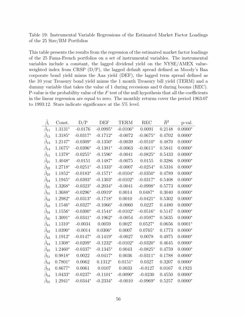
Table 19: Instrumental Variable Regressions of the Estimated Market Factor Loadingsof the 25 Size/BM Portfolios

This table presents the results from the regression of the estimated market factor loadingsof the 25 Fama-French portfolios on a set of instrumental variables. The instrumentalvariables include a constant, the lagged dividend yield on the NYSE/AMEX value-weighted index from CRSP (D/P), the lagged default spread defined as Moody’s Baacorporate bond yield minus the Aaa yield (DEF), the lagged term spread defined asthe 10 year Treasury bond yield minus the 1 month Treasury bill yield (TERM) and adummy variable that takes the value of 1 during recessions and 0 during booms (REC).P-value is the probability value of the F test of the null hypothesis that all the coefficientsin the linear regression are equal to zero. The monthly returns cover the period 1963:07to 1993:12. Stars indicate significance at the 5% level.

βi Const. D/P DEF TERM REC R2 p-val.

β11 1.3131∗ -0.0176 -0.0995∗ -0.0106∗ 0.0091 0.2148 0.0000∗

β12 1.3185∗ -0.0317∗ -0.1712∗ -0.0072 -0.0675∗ 0.4702 0.0000∗

β13 1.2147∗ -0.0309∗ -0.1350∗ -0.0039 -0.0510∗ 0.4870 0.0000∗

β14 1.1675∗ -0.0396∗ -0.1381∗ -0.0063 -0.0611∗ 0.5841 0.0000∗

β15 1.1378∗ -0.0255∗ -0.1596∗ -0.0041 -0.0825∗ 0.5433 0.0000∗

β21 1.4048∗ -0.0151 -0.1487∗ -0.0075 0.0155 0.3286 0.0000∗

β22 1.2718∗ -0.0251∗ -0.1333∗ -0.0007 -0.0254∗ 0.5316 0.0000∗

β23 1.1852∗ -0.0183∗ -0.1571∗ -0.0104∗ -0.0350∗ 0.4789 0.0000∗

β24 1.1945∗ -0.0393∗ -0.1303∗ -0.0102∗ -0.0317∗ 0.5408 0.0000∗

β25 1.3268∗ -0.0323∗ -0.2034∗ -0.0041 -0.0998∗ 0.5773 0.0000∗

β31 1.3688∗ -0.0296∗ -0.0919∗ 0.0014 0.0487∗ 0.3040 0.0000∗

β32 1.2982∗ -0.0313∗ -0.1718∗ 0.0010 -0.0421∗ 0.5302 0.0000∗

β33 1.1546∗ -0.0327∗ -0.1066∗ -0.0060 0.0227 0.4480 0.0000∗

β34 1.1556∗ -0.0300∗ -0.1544∗ -0.0102∗ -0.0516∗ 0.5147 0.0000∗

β35 1.3091∗ -0.0341∗ -0.1962∗ -0.0054 -0.0597∗ 0.5635 0.0000∗

β41 1.1310∗ -0.0034 0.0059 0.0027 0.0527∗ 0.0656 0.0001∗

β42 1.0390∗ -0.0014 0.0306∗ 0.0007 0.0765∗ 0.1773 0.0000∗

β43 1.1912∗ -0.0147∗ -0.1419∗ -0.0027 0.0078 0.4975 0.0000∗

β44 1.1308∗ -0.0209∗ -0.1232∗ -0.0102∗ -0.0320∗ 0.4645 0.0000∗

β45 1.2460∗ -0.0337∗ -0.1345∗ 0.0043 -0.0825∗ 0.4759 0.0000∗

β51 0.9818∗ 0.0022 -0.0417∗ 0.0036 -0.0311∗ 0.1788 0.0000∗

β52 0.7801∗ 0.0062 0.1312∗ 0.0151∗ 0.0327 0.3207 0.0000∗

β53 0.8677∗ 0.0061 0.0107 0.0033 -0.0127 0.0167 0.1923

β54 1.0433∗ -0.0237∗ -0.1101∗ -0.0090∗ -0.0230 0.4550 0.0000∗

β55 1.2941∗ -0.0344∗ -0.2334∗ -0.0010 -0.0969∗ 0.5257 0.0000∗

56

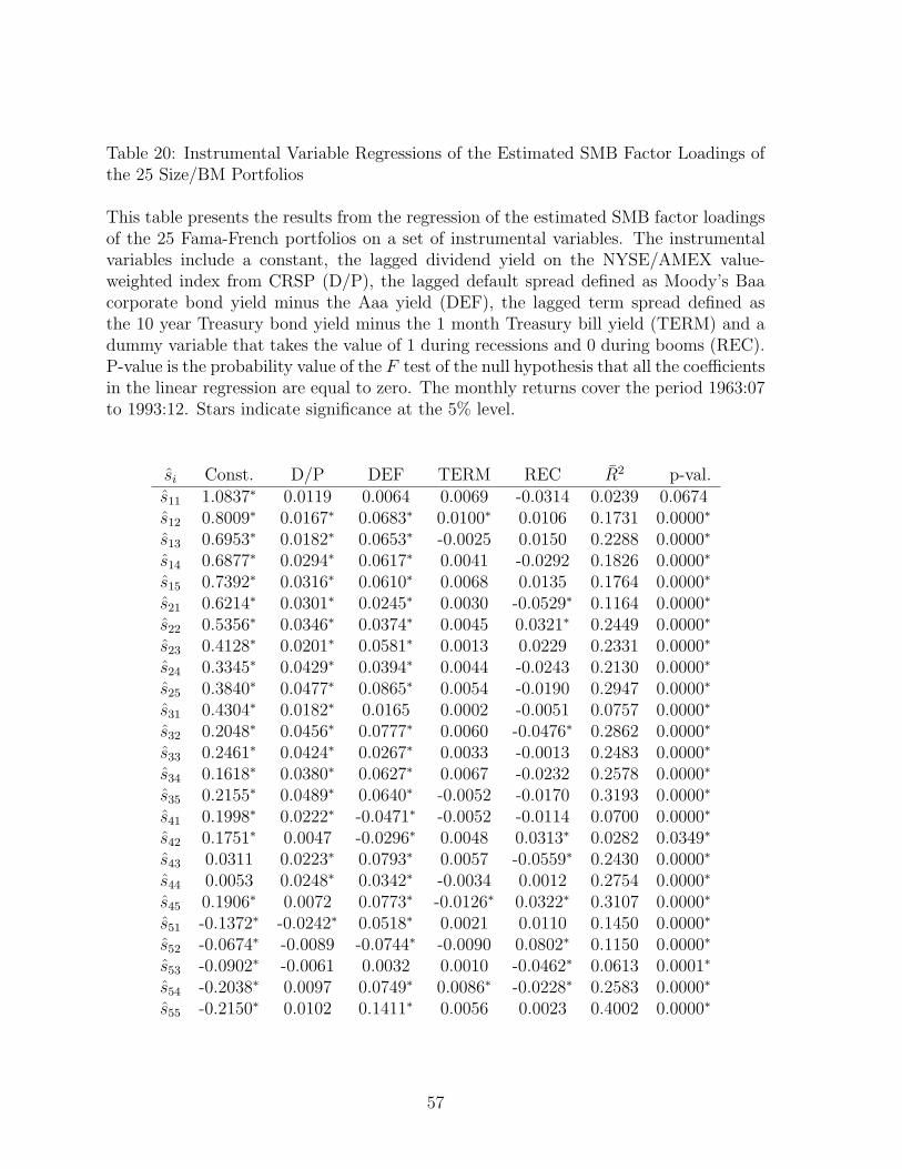
Table 20: Instrumental Variable Regressions of the Estimated SMB Factor Loadings ofthe 25 Size/BM Portfolios

This table presents the results from the regression of the estimated SMB factor loadingsof the 25 Fama-French portfolios on a set of instrumental variables. The instrumentalvariables include a constant, the lagged dividend yield on the NYSE/AMEX value-weighted index from CRSP (D/P), the lagged default spread defined as Moody’s Baacorporate bond yield minus the Aaa yield (DEF), the lagged term spread defined asthe 10 year Treasury bond yield minus the 1 month Treasury bill yield (TERM) and adummy variable that takes the value of 1 during recessions and 0 during booms (REC).P-value is the probability value of the F test of the null hypothesis that all the coefficientsin the linear regression are equal to zero. The monthly returns cover the period 1963:07to 1993:12. Stars indicate significance at the 5% level.

si Const. D/P DEF TERM REC R2 p-val.s11 1.0837∗ 0.0119 0.0064 0.0069 -0.0314 0.0239 0.0674s12 0.8009∗ 0.0167∗ 0.0683∗ 0.0100∗ 0.0106 0.1731 0.0000∗

s13 0.6953∗ 0.0182∗ 0.0653∗ -0.0025 0.0150 0.2288 0.0000∗

s14 0.6877∗ 0.0294∗ 0.0617∗ 0.0041 -0.0292 0.1826 0.0000∗

s15 0.7392∗ 0.0316∗ 0.0610∗ 0.0068 0.0135 0.1764 0.0000∗

s21 0.6214∗ 0.0301∗ 0.0245∗ 0.0030 -0.0529∗ 0.1164 0.0000∗

s22 0.5356∗ 0.0346∗ 0.0374∗ 0.0045 0.0321∗ 0.2449 0.0000∗

s23 0.4128∗ 0.0201∗ 0.0581∗ 0.0013 0.0229 0.2331 0.0000∗

s24 0.3345∗ 0.0429∗ 0.0394∗ 0.0044 -0.0243 0.2130 0.0000∗

s25 0.3840∗ 0.0477∗ 0.0865∗ 0.0054 -0.0190 0.2947 0.0000∗

s31 0.4304∗ 0.0182∗ 0.0165 0.0002 -0.0051 0.0757 0.0000∗

s32 0.2048∗ 0.0456∗ 0.0777∗ 0.0060 -0.0476∗ 0.2862 0.0000∗

s33 0.2461∗ 0.0424∗ 0.0267∗ 0.0033 -0.0013 0.2483 0.0000∗

s34 0.1618∗ 0.0380∗ 0.0627∗ 0.0067 -0.0232 0.2578 0.0000∗

s35 0.2155∗ 0.0489∗ 0.0640∗ -0.0052 -0.0170 0.3193 0.0000∗

s41 0.1998∗ 0.0222∗ -0.0471∗ -0.0052 -0.0114 0.0700 0.0000∗

s42 0.1751∗ 0.0047 -0.0296∗ 0.0048 0.0313∗ 0.0282 0.0349∗

s43 0.0311 0.0223∗ 0.0793∗ 0.0057 -0.0559∗ 0.2430 0.0000∗

s44 0.0053 0.0248∗ 0.0342∗ -0.0034 0.0012 0.2754 0.0000∗

s45 0.1906∗ 0.0072 0.0773∗ -0.0126∗ 0.0322∗ 0.3107 0.0000∗

s51 -0.1372∗ -0.0242∗ 0.0518∗ 0.0021 0.0110 0.1450 0.0000∗

s52 -0.0674∗ -0.0089 -0.0744∗ -0.0090 0.0802∗ 0.1150 0.0000∗

s53 -0.0902∗ -0.0061 0.0032 0.0010 -0.0462∗ 0.0613 0.0001∗

s54 -0.2038∗ 0.0097 0.0749∗ 0.0086∗ -0.0228∗ 0.2583 0.0000∗

s55 -0.2150∗ 0.0102 0.1411∗ 0.0056 0.0023 0.4002 0.0000∗

57

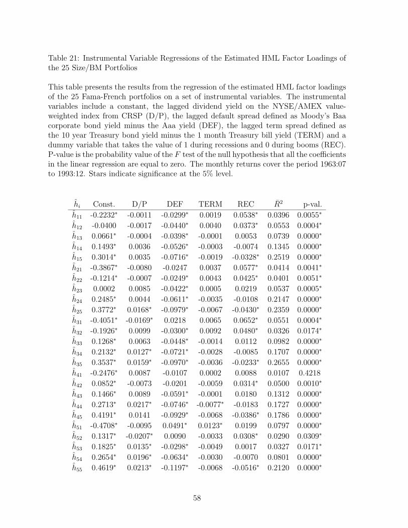
Table 21: Instrumental Variable Regressions of the Estimated HML Factor Loadings ofthe 25 Size/BM Portfolios

This table presents the results from the regression of the estimated HML factor loadingsof the 25 Fama-French portfolios on a set of instrumental variables. The instrumentalvariables include a constant, the lagged dividend yield on the NYSE/AMEX value-weighted index from CRSP (D/P), the lagged default spread defined as Moody’s Baacorporate bond yield minus the Aaa yield (DEF), the lagged term spread defined asthe 10 year Treasury bond yield minus the 1 month Treasury bill yield (TERM) and adummy variable that takes the value of 1 during recessions and 0 during booms (REC).P-value is the probability value of the F test of the null hypothesis that all the coefficientsin the linear regression are equal to zero. The monthly returns cover the period 1963:07to 1993:12. Stars indicate significance at the 5% level.

hi Const. D/P DEF TERM REC R2 p-val.

h11 -0.2232∗ -0.0011 -0.0299∗ 0.0019 0.0538∗ 0.0396 0.0055∗

h12 -0.0400 -0.0017 -0.0440∗ 0.0040 0.0373∗ 0.0553 0.0004∗

h13 0.0661∗ -0.0004 -0.0398∗ -0.0001 0.0053 0.0739 0.0000∗

h14 0.1493∗ 0.0036 -0.0526∗ -0.0003 -0.0074 0.1345 0.0000∗

h15 0.3014∗ 0.0035 -0.0716∗ -0.0019 -0.0328∗ 0.2519 0.0000∗

h21 -0.3867∗ -0.0080 -0.0247 0.0037 0.0577∗ 0.0414 0.0041∗

h22 -0.1214∗ -0.0007 -0.0249∗ 0.0043 0.0425∗ 0.0401 0.0051∗

h23 0.0002 0.0085 -0.0422∗ 0.0005 0.0219 0.0537 0.0005∗

h24 0.2485∗ 0.0044 -0.0611∗ -0.0035 -0.0108 0.2147 0.0000∗

h25 0.3772∗ 0.0168∗ -0.0979∗ -0.0067 -0.0430∗ 0.2359 0.0000∗

h31 -0.4051∗ -0.0169∗ 0.0218 0.0065 0.0652∗ 0.0551 0.0004∗

h32 -0.1926∗ 0.0099 -0.0300∗ 0.0092 0.0480∗ 0.0326 0.0174∗

h33 0.1268∗ 0.0063 -0.0448∗ -0.0014 0.0112 0.0982 0.0000∗

h34 0.2132∗ 0.0127∗ -0.0721∗ -0.0028 -0.0085 0.1707 0.0000∗

h35 0.3537∗ 0.0159∗ -0.0970∗ -0.0036 -0.0233∗ 0.2655 0.0000∗

h41 -0.2476∗ 0.0087 -0.0107 0.0002 0.0088 0.0107 0.4218

h42 0.0852∗ -0.0073 -0.0201 -0.0059 0.0314∗ 0.0500 0.0010∗

h43 0.1466∗ 0.0089 -0.0591∗ -0.0001 0.0180 0.1312 0.0000∗

h44 0.2713∗ 0.0217∗ -0.0746∗ -0.0077∗ -0.0183 0.1727 0.0000∗

h45 0.4191∗ 0.0141 -0.0929∗ -0.0068 -0.0386∗ 0.1786 0.0000∗

h51 -0.4708∗ -0.0095 0.0491∗ 0.0123∗ 0.0199 0.0797 0.0000∗

h52 0.1317∗ -0.0207∗ 0.0090 -0.0033 0.0308∗ 0.0290 0.0309∗

h53 0.1825∗ 0.0135∗ -0.0298∗ -0.0049 0.0017 0.0327 0.0171∗

h54 0.2654∗ 0.0196∗ -0.0634∗ -0.0030 -0.0070 0.0801 0.0000∗

h55 0.4619∗ 0.0213∗ -0.1197∗ -0.0068 -0.0516∗ 0.2120 0.0000∗

58

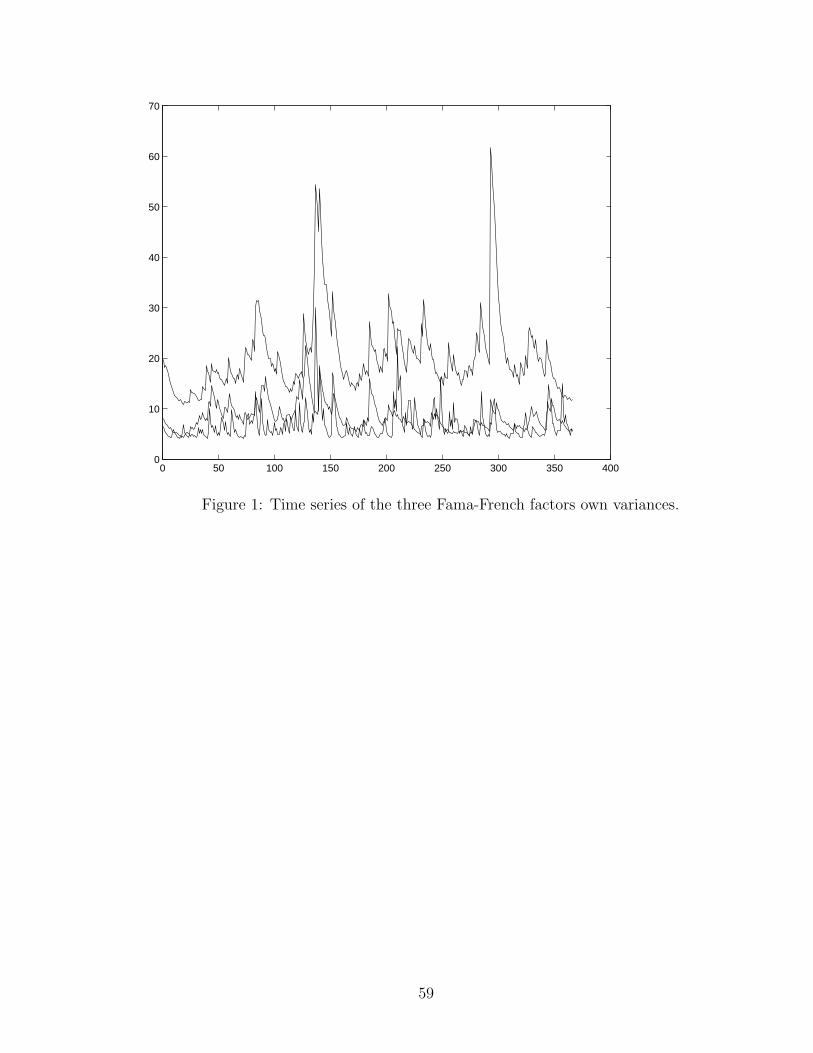
0 50 100 150 200 250 300 350 4000

10

20

30

40

50

60

70

Figure 1: Time series of the three Fama-French factors own variances.

59

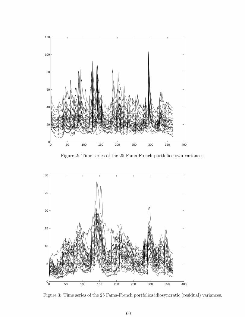
0 50 100 150 200 250 300 350 4000

20

40

60

80

100

120

Figure 2: Time series of the 25 Fama-French portfolios own variances.

0 50 100 150 200 250 300 350 4000

5

10

15

20

25

30

Figure 3: Time series of the 25 Fama-French portfolios idiosyncratic (residual) variances.

60

a dynamic asset pricing model with time-varying … gerber - dynamic asset...a dynamic asset pricing...

Documents