Testing Asset Pricing Models With Coskewness

Giovanni BARONE AOESIInstitute of Finance, University of Lugano, Lugano, Switzerland (giovanni,barone-adesi@/u.unisi.ch)

Patrick GAGLIAROI NIInstitute of Finance, University of Lugano, Lugano, Switzerland (patrick.gagliardini@/u.unisi.ch)

Giov an ni URGAFaculty of Finance, Cass Business School, London, U,K. (g.urga@city ac.uk)

In this article we investigate portfoli o cos kcwnc ..s using a qua dnuic market model as a rerum -generati ngproce ss. We show that the portfolio, of small /lar ge ) firm ... have negative (positive ) coskcwncss with themarket. We tcs\ an asset pricing model includ ing coskcwncss by checking the validity of the restriction sthat it impo ...ex on the return-generatin g process. \1./1.' find evidence of an addi tional component in expectedC:(CC'iS return .... which i ... nor explained by either covariance or cos kcwncss with the market. However,

thi... unexplain ed compo nent i... homogeneous :lcrOSS portfol ios in our sample and modest in magnitude,

Finall y, we investigate the implication s of erroneously neglecting coskcwncss for testin g a...se t pricin g

model... , with particular attention to the empirica lly detected exp lana tory power of linn ... ize.

KEY WO RDS : Asset pricing ; Asymp totic least squares : Co skewuc ss: Generali zed method of moments;~lonlt' Car lo simulation.

1. INTRODUCTION

Asse t pn cmg models generally express expected returnson financial asse ts as linear functions of co variances of re­turns with some systema tic risk facto rs, Several formul ation sof this genera l parad igm have been proposed in the litera­ture (Sharpe 1964 : Lint ner 1965: Black 1972: Merton 1973:Rubin stein 1973 : Kraus and Litzenberger 1976: Ross 1976:Breeden 1979: Barone Adesi and Talwar 1983: Barone Adesi1985: Jagannathan and Wang 1996 : Harvey and Siddique 2000:Dittmar 2002). However. most of the empirica l tes ts sugges tedto date have produ ced negat ive or ambiguous res ults. Thesefindings have spurred renewed interest in the statistical prop·erties of the currently available testi ng methodologies. Amongrece nt studies. Shunken ( 1992) and Kan and Zhang 11999a. h)analyzed the common ly used stat istica l methodologies andhighli ghted the sources of ambig uity in their I1nd ings.

Although a full speci ficat ion of the return-generating processis not needed for the formu lation of most asse t pricing mod­els. it appears that only its a priori knowledge may lead to thedes ign of reliable tests, Because this condition is neve r met inprac tice. researchers arc forced to make unpalatable cho ices be­tween two altern ative approac hes. On the one hand. powerfultests ca n be designed in the co ntext ofa (fully) specifie d return­genera ting process. hut they arc misleadin g in the presence ofpossible model misspecificat ions. On the other hand . more to l­era nt tests may be co nsidere d. hut they may not be powerful.as noted by Kan and Zhou (1999) and Jagannathan and Wang(200 1I. Note that the first cho ice may lead not only to the rejec­tion of the co rrect model , but also to the acceptance of irrc lc­vant factors as sources of systematic risk. as noted by Kan andZhang ( 1999a .h).

Tn complicate the pict ure. a numb er or empirical regul aritieshave been detected that arc not consistent with standa rd asse tpricing mod els. such as the mean-var iance capi tal asse t pricingmodel (CA PM I. Amo ng other stud ies, Bunz ( 198 1) re lated ex­peered returns to firm size. and Fama and French (1995) linkedexpected returns also to the rurio of book value to mar ket value,

Alth ough the persistence of these anomalies ove r time is sti llsubject to debate. the evidence suggests that the mean-varianceCAPM is not a satisfac tory description of market equilibrium.These pricing anomalies may be relat ed to the possibility thaiuse less factors appea r to be priced. Of course. it is also possi­hie that pricin g anomalies arc due to omitted factors. Alth oughstatistica l tests do not allow us to choose between these twopossibl e explanations of pricin g anoma lies. Kan and Zhang( 1999a.h) sugges ted that perhaps a large increment in R2 andthe per sistence or sign and size of coe fficie nts over time aremost likely to be associated with trul y priced factors.

In the light of the forego ing. the aim of this article is toconsider market cos kew ncss and to investigate its role in test­ing asse t pricing models. A dataset of monthly return s on10 stock port folios is used . Following Harvey and Siddique(2000) . an asse t is defined as having "positive cos kewness' withthe market when the res iduals of the regression of its returnson a co nstant and the market return s are positive ly co rrelatedwith squared market returns, Therefore. an asset with positi ve(negative) cos kewness reduces (inc reases) the risk of the por t­folio to large absolut e market returns. and should comma nda lower (hig her>expected return in equilibrium.

Rubin stein ( 1973). Kraus and Litzenberger (1976). BaroneAdcs i ( 1985). and Harvey and Siddique (2000) studied non ­norm al asse t pricing models related to cos kew ness . Krausand Litzenb erger ( 1976) and Harvey and Siddique (2000)formul ated expected returns as a function of covariance andcoskewness with the market port folio, In particular. Harveyand Siddique (2000 ) assessed the importance of coskewnessin explaining expected returns by the increment of R2 in cross ­sectional regress ions. More recen tly. Dittm ar (2002 ) presenteda framework in which age nts are a lso adve rse to kurtosis. irn­plying that asse t retu rns are influenced by bot h coskcwness andcok urtos is with the return on agg rega te wea lth, The author tests

© 2004 Am erican Stat istical Associat ionJournal of Business & Econ om ic Stati sti cs

Octo be r 2004 , Vol . 22, No. 400110.11 98/07350010 400 000 0244

474

Barone Adesi, Gagliardini, and Urga: Coskewness in Asset Pricing 475

2.1 The Quadratic Market Model

( 2)

( I )

I = I. . .. . 1'.r , = a + fJrM" + e .,

H i .: y = II in (1) .

H I' : y E]RN

where a is a N x I vector o f inte rcepts. fJ and y are N x I vec­

tors of sens itivities. and e , is an N x I vector of errors satisfying

E[E/IRM.,. Rr ./ ] = II.

with R,'l,' " and R"'.t denoting all presen t and past values ofRM., and R,.../.

Th e quad ratic mark et model is a direct ex tension o f the we ll­known rnarket mo del tSha rpc 1964 : Lintn er 1965 ). which cor­responds to rest riction y = 0 in ( I).

Fac tor mode ls arc among the mosl widely used return­ge nerating pro cesses in financi al econome trics, Th ey explaincomoverne nts in asset return s as arising fro m the co mmo n ef­fect of a (s mall) number of underl ying vari able s, ca lled factors(sec . e .g.. Ca mpbe ll. 1.0. and MacK inlay 1987: Gourieroux andJasiak 200 1). In thi s article we use a linear two-factor mod e l.the qu ad ratic market mod el. as a return-generating process.Market retu rns and the square of the mark et returns are the twofactor s. Specifica lly. we denote by R, the N x I vector of return sin pe riod t of N portfolios and by R,H.I the return of the market.If R F.t is the re turn in pe riod t of a (conditionally) rivk-freeass et. then port fol io and market excess ret urns are de fined by

r . = Rt - R,...,l and r,H.' = RM., - R,.." . whe re l is a N x I vecto rof ls. Similar ly. the excess squared market retu rn is defined by

liM,' = R,~J , ' - RF.I ' Th e quadratic market mod el is specified by

r/ =a +{3rM., +YQM.I + E,. t= 1• •••• 1'.

The motivat ion for including the square of the mar ket retu rnsis to fully acco unt for coskewness with the mark et port folio .In fact. dev iations from the linear re lation betwee n asset return sand market returns implied by (2) arc e mp irica lly observed.More spec ifica lly, for some c lasses of assets. residu als fro m theregression of returns on a constant a nd market returns ten d to bepositive ly (neg atively ) corre lated with squared mark et returns.These assets there fore show a tenden cy to have re lat ivel y high er(lowe r) retu rns whe n the mark et expe riences high absolute re­turn s. a nd arc sa id to have positive (negative ) coskewncss withthe mark et. Thi s findi ng is supported by OUT empirical inves­tigation s in Sect ion 4 . whe re. in accorda nce with the resu ltsof Harvey and S iddiquc (2000 ). we lind that portfolios formedby asse ts of sma ll fir ms te nd to have negat ive cos kewncss withthe market . wherea s port fo lios formed by assets o f large firm shave positive market cos kcwness. In addition to class ical beta .market cos kewncs s is there fore a nother importan t risk churuc­tcristic : all asset tha t has positi ve cos kcwn css with the mar ketdiminishes the sens itivity of a portfol io to large ab solute ma r­kct returns . Th erefore . everything e lse hein g eq ua l. investor sshould pre fer asse ts with positi ve market cos kewness to thosewi th negat ive co skewness. Th e qu adrat ic market model ( 1) isa spec ification that pro vides us with a very simple way to takeinto account mark et cos kcwncss. Indeed. we have

1 ,y =~[E I covlc.. R,i l.t l. (3 )

".1

In this section we introdu ce the econo metric spec ificationsco ns idered in the artic le. \Ve describe the return-gen erat ingprocess. deri ve the corres ponding restr icted equ ilibri um mod ­e ls. and finall y compare OUT approac h with a G MM fra mework.

an ex te nded asset pricing model within a ge neral ized methodof mom ent s (G!\l M ) framework (see Han sen 1982).

Most of the foregoin g formulations are very ge nera l. becau sethe specification of an underl ying return-ge nerating process isno t requ ired . However , we arc conce rned about their possiblelack of pow er. made worse in this context by the fac t that co ­varia nce and coskcwness with the market arc a lmo st perfect lycollinear across port foli os. Of course . in the ex treme case.in whic h market cov ariance is proportion al to market cos kcw­ness. it will be imp ossibl e to identify covariance and coskew­ness premia separately. Th ere fore . to ident ify and acc uratelymeasu re the co ntr ibution of cuskcwncss. in thi s art icle we pro­pose an approa ch (sec also Baron e Ade si 19X5) based o n theprio r specification of an appro pria te return -generat ing process.the qu ad rat ic market mod el. Th e quadr at ic market mo de l i ~ anextension of the tradit ion al mark et mo de l (Sha rpe 1964; Li ntne r1965). including thc ' quare of the market returns as an add i­tional facto r. The coefficien ts of the qu adr at ic factor measurethe margin al contribution of co skew ness to expec ted excess re­turns . Becau se mark et returns and the square of the mark etret urns are a lmo st orthogo nal regressor s. we obtain a precisetest of the significance of quadrat ic coefficients. In add ition .thi s fra mework a llows us to test an as set pricing mod el withcoskewness by chec king the restricti on s that it imposes on thecoeffic ie nts of the quad rati c market mod el. Th e spec ificationof a ret urn -generat ing process provid es more powerful tests. asco nfir med in a series of Mon te Ca rlo simulations (see Sec . 5).

In addi tion to eva luating asset pri cing mod el s that includecoskewncss. it is a lso important to investigate the co nseq uenceson asset pricin g tests when coskew ness is erroneo usly omit­ted . \Ve consider the possib ili ty tha t port folio characteristics ,suc h as size. arc e mp irically found to explain ex pec ted ex ­cess ret urn s because or the o missio n of a trul y priced factor.nam ely coskcwness . To explain this prob lem. le t us assume thatcoskcwness is trul y priced but is omitted in an asset prici ngmod el. Th en. if market cos kcwncs s is corre lated with a variablesuc h as size. this var iable will have spurious explanatory powerfor the cross-section of ex pected returns. because it pro xies fo romitted coskcw ness. In our empirica l applica tion (sec Sec . 4 ).we ac tually tind tha t co skcwness a nd firm size are corre lated .This finding sugg es ts that the e mp irically observed relation be­tween size and asse ts excess returns may he explained by theomissio n of a systematic ris k factor. namel y mark et co skew nes s(see also Harvey and Sidd iqu c 2000. p. 1281).

Th e art icle is orga nized as follows. Sectio n 2 int rodu cesthe qu adr ati c mark et mod el. A n asse t pricin g model inc lud ingcos kcwness is der ived usin g arbitrage pricing. and the testingof various related statistica l hypotheses is d iscussed . Sect ion .3reports est ima tor s and test statistics used in the e mp irical partof the art icle. Secti on 4 descri bes the data and rep ort s em pirica lresults. Secti on 5 provides Monte Car lo simulations for inves­tigating the tinit e sample pro pert ies of our te st statis tics . andSec tion 6 concludes .

2. ASSET PRICING MODELS WITH COSKEWNESS

476 Journal of Business & Economic Statistics . Octobe r 2004

(6)

H, ; 3 ,1 : 0' = lI y in t l ).

2.2 Restricted Equilibrium Models

(9)

(1)

(8)I = I. .... T .

/;'[ r,III,l o)J = u,

r, = 13 1".11., + Y'I.II ., + y ll + AO I + ' "H~ ; 3 1J. AO; 0' = IIy + AOI in II).

E( r,) = l AO + 13 )., + y A ~ .

correspondi ng (0 the specification

Asset pricin g mod els of the type (4) have been conside redby Krau s and Litze nberge r ( 1976) and Har vey and Sidd ique(2000) . Har vey and Sidd ique (2000) int rodu ced the ir specifi­ca tion as a model in whic h the stoc has tic d isco unt fac to r isquadra tic in mark et re turns . Specifica lly. in our nota tion. theasse t pricing mo de l with coskewness (4) is equivalent to the or­thogonal ity co ndition

where the stoc has tic di scount fac tor mdtS ) is given hy m,( e5) =I - I'M .181 - tJJ/ .,tJ2 a nd e5 = (8]. (5 :!) is a two-d imension al pa ra ­meter. A quadratic stochas tic di scount fact or 111 ,(e5) ca n he j usti­fied as a (formal) second-order Taylor ex pansion of a stochas ticdi scount facto r, whic h is no nlinear in the market re tu rns . Thu sin the GMM a pproach. the derivation and tes ting of the o rthog­onali ty condi tion (9) do l10t requ ire a prior speci fica tio n o f adata-gen eratin g pro cess.

More recent ly. in a con dit ional G Mt\.1 fram ework. Dit tmar(2002) used a stoc hast ic di scount fa, tor mode l embodyi ng hot hquadratic and cubic terms. Th e va lidi ty of the mode l is tes tedby a G~H\t sta tis tic using the we ighti ng matr ix proposed byJagannathan and Wan g (1996) and Han sen and Jagarmathan( 1997). As ex plained earlier. the main cont ribu tion of our ar­ticle . beyond the re sult s obtained hy Har vey and Sidd ique(2000) and Dittmar (2002). is that we foc us 0 11 te sti ng the as­se t prici ng model w ith coskcwness (4) th rough the res trict io nsthat it imposes 0 11 the return-gen eratin g process ( I ). instead o fado pt ing a meth odology us ing an uns peci fied a lternat ive (e .g ..a G M M test) .

2.3 The Generalized Method of Moments Framework

Specif ica tion (8) co rres po nds to the case where the fac to r omit­ted in model (4) has hom ogeneou s se nsitivit ies across portfo­lios. Fro m (7). Ao may be int erpreted as the expected excessre turns of a port foli o wit h covaria nce and cos kcwncss with themark et both equal to O. Such a portfo lio may correspond tothe ana logous of the zero-be ta portfoli o in the Black ve rsio nof the ca pita l asset prici ng model t fl luck 1972 ). Alte rna tively.AO > 0 (Ao < 0) may he du e to the lise of a risk-free rate lower(hig he r) than the act ua l ra te faced by inves to rs . Wi th referenceto the observed em pirical regul arities and mod el miss pec itica ­tio ns ment ioned in Sectio n I. the imp ort ance of model (8) istha t i f hypo thesis H :! is not rejec ted agains t Hr, then we ex pec tpo rtfo lio c ha rac te ristics suc h as size to not have add itio na l ex­plana tory power for expec ted excess ret urn s. once coskcw ncssis taken into account. In add itio n. a more powerful evalua tionof the va lidi ty of the asse t pricing mode l (4 ) shou ld he providedby a test of HI agai nst the alte rnative 'H:! .

us wit h informati on about the sens itivi ties of our port foli os tothi s factor. Furthe rmore. variab les represent ing portfolio cha r­ac teristics. which are correlated with ii across portfo lios. willhave sp ur ious ex plana tory power for expected excess returns.because they are a proxy for the se nsitivit ies to the omi ttedfacto r. A case of part icular inte rest is whe n a is hom ogen eou sacross assets. ii = Aot. where Ao is a scalar. that is.

(4)

(5)

I = I. .... T.

A, = £1,-.11.,) .

El r,) = 13).1+ y A~ .

Th ere fore. the asset pricin g model with coskewness (4) is testedby test ing 'H I aga inst Hr·

When model (4) is not supported by data. there exis ts anadditional co mponent a (a N x I vect or) in ex pected excessreturns that ca nnot he fully related to mark et risk and coskew­ness risk. E( r ,) = f3 AI + y i.~ + a . In this case. intercepts a ofmodel ( 1) sat isfy a = ()y +a. It is crucia l to inves tigate howthe addit ional co mpo nent a varies across asse ts. lndccd , if th iscompone nt arise s from an omit ted fac tor. the n it w ill provide

where i'l and A:! arc expected excess ret urn s o n portfo lioswhose excess returns arc pe rfectly co rrelated wit h factors1)1. t and «.\1. t . Eq uat ion (4) is in the for m of a ty pical linearasset prici ng mode l. which re lates expected excess re tu rns tocovarianccs and coskew nes xes w ith the market. In this articlewe tes t the assc r pricing model with coskewncss (4) throu ghthe restr iction s that it im pose- on the coefficients of the return­genera ting process ( I ). We derive these restr ictions. Becau sethe e xcess market re tu rn ru, sutis tiex (4). it must he that

From the standpoi nt of financial econo mics. a linear Iac ­tor mo de l is only a return -generating process. which is notnecessa rily consistent with notion s of economic eq uilib rium,

Const ra ints on its coeffic ients arc imposed for exa mple by arbi ­trage pr ic ing IRoss 1976; Chamberlai n and Rothschil d 1983).The arbitrage pricin g theory impli es tha t e-x pec ted excess re­tu rns of asse ts fo llow ing the fac tor model ( I) sa tisfy the restric­tio n (Barone Ade si 1985 )

where I I (rcsp, ( " .1) arc the rcsidualv fro m a theoret ical re­

gression of portfolio returns R, (market square returns Hi l ,l'resp.) on a constant and market return HM" . Because coef­ficien ts y arc pro portiona l to co vle .. R~I.tI . we ca n lise thees tima te of y in model ( I ) to investigate the coskcw nesspro pert ies of the N portfo lios in the sa mple. Moreover. al­though y docs not correspo nd exactly 10 the us ua l probabilist icdefinit ion of market co skcwncss. coe fficien t y is a very goodproxy for cnvt r .. R~f.t ) / V (R.~f . t ) ' as po inted out by Kra us andLitzen be rger ( 1976). With in our samp le. the approx ima tion er­ror is sma lle r than I fh (sec App. A) , Finall y. the statis tical( jo int ) sign ifica nce of co skcwncss coe fficie nt y call be assessedhy testin g the null hypo thesis H;. against the a lternat ive Hr .

A similar restrict ion does not ho ld for the second fac tor lIM .t

because it is not a traded asse t. However , we expect i .:! < O.because assets wi th posit ive coskcwncxs decrease the risk of aportfo lio wit h res pect to large absolute mark et return s and thu ssho uld comma nd a lower risk premi um in an arbitrage equ ilih ­rium, By taking expectations on ho th sides of ( I ) and subst i­tuting (4 ) and (5) . we deduce tha t the asset pricing mod el (4)

impl ies the cross-e qua tion restrict io n a = (Jy . whe re I? is thescalar pa rame ter () = ). :! - £'((/'\1 ./). Th us ar bitrage pricin g isco nsiste nt wit h the restricted model

L

Barone Aoest. Gagliardini, and Urga: Coskewness in Asset Pricing 477

where

1\ 4 1

r = J. ... . T.

where F, = ( I . rv» q.H ,t )'.Let u... now conside r the test of the (joi nt) ... tati st ica! sig ­

niticunce of the cos kewncss coe fficie nts y . th at is the test ofhyp oth e sis 'H;'.: y = Il . again ... t N·F. Th is test ca n he easilyperformed co mputing a \Vald sta tis tic . which is g iven by

,t. _ ·I·_I_ _ , ~ - I ­c;r - -." y L. y.

~-­t

As is well known. the Pi\I L estimator for la'. ff . y ' )' is equiv­alent to the geucralized lea ...t squares (GLS ) c ... tirnator o n the

SU R ...ystem and also to the ordinary least ...quare ... t (O LS) esti­mato r performed equation hy equation in model (I ). LeI n de­

note the N x 3 matrix defined bv II = la Ii Y I. T he P~l L

c ...timator ii = Iii P 91is consisten t when T - oc, and itsasymptotic di...tribution is given hy

(Upper indi ces in a matrix denote clements of the inversc.)Th e

sta tis tic ~r* is asymptotica lly X2("l -distrihuled . with" = N.whe n T - 00.

\\ here vccht I ) is a (N~l )N x I vec tor representation of I co n­

raining o nly cleme nt... o n and above the mai n d iagonal. Th ePxll. est imator of (J based on the norma l fami ly is ob ta ined by

maximizing

1101

\Vc a"..urne that the error term £1 in model (I) with 1 =I . . . . . T is a homo..ccda...tic martingale difference -cqucnce

...ati'ifying:

3. ESTIMATORS AND TEST STATISTICS

I:'[E/£; I£/_I . R,H" . RF.I ] = I .

where I i ... a po ... hive-definite N x N matrix. T he fac tor

f, = (",H." C/ ," ',) ' is -uppo...cd 10 he exogenous in the sen-eo f Eng le. Hendry. and Rich ard (1988). Th e expecta tio n and

the var iance-covariance matri x of fac tor r, arc den ot ed byJi and I f. Suui-t icul inference in the ass et pr icing models pre­se nted in Sect ion 2 is co nve niently cas t in the ge ne ra l fram e­

work of Pt\lL methods (While 1981 ; Gouri croux , M onfor t, and

Trogn on 1984 ; Boller-l ev and Wooldridge 199 2). If (I denotes

the parameter of intere st in the model und er con- ideration. the nthe PML es tima tor b defined by the ma xim izat io n

3.1 The Pseudo-Maximum Likelihood Estimator

In this sect io n we der ive the es tima tors and test sta tistic :">

used in our empirical ap plicat io ns . Foll owing an approach

widely adopted in the literature (sec. c.g.. Campbe ll et al. 1987:Gouricroux and Javiuk 200 I ). we conside r the ge neral frame ­

work of p..cudo- rnaximum likel ihood ( P~ 1 L) methods, \Ve de ­

rive the stativtical properties of the estimators and test statisticswithin the different co ... kcwnes... a ......ct pri ci ng models pre ...cntcd

in Section 2.1 and 2.2. For co m plete ness. we provide full

derivation in the Appendixes.

II = arg ma x L r( Hl."

I I I) 3.3 Restricted Equilibrium Models

T he P~lL estimator (j i ... g ivcn hy the fo llowi ng ...y... tem of im ­plici t equations (sec App. B):

We now consider the- co ns tra ined models (6) a nd (8) deri ved

by arbitrage eq uili br ium. The est imat ion of these models is lcs...simple. bccau...c they e ntai l cross-eq uation revtrictions . We let

" (Q' '" . h(" )' )'u = " .y . ". AU. 'ee L. •

denote the vector of parameters of model (S) . The P~1L. est ima­tor of iJ ba-ed on a normal pseudo-conditional log -likeli hood isdefined by minimization of

( 16)

r=J. ... . T.

(

T ) ( r )-tCp'·Y')' = Dr,- i:',<I ii; L ii ,ii;1=1 ,=1

E,(O) =r, - {J r.\f ,' - Yc/'\I ., - y lJ - i.ol.

where the c rite rio n l. r UIl is a (condit iona l) pse udo -log-likeli­

hood. More specifical ly. Lr IO) is the (co ndit iunal} log ­

likeli hood of the mode l when we adopt a g iven conditional

d istribu tion for error E, that satisfies ( 10) a nd is such that

the rc-ulting p...cudo-truc density of the model is exponentialquadratic . Under ... tandurd regularity a ...surnptions. the P~1L c ...­timator (i i..consistent for any chosen condit ional di ... tribution of

error e , ...ati ... fvin g the foregoing condition ... ( ...cc the aforemen ­

tio ned references}. Estimator 1i is efficient when the P...cudo­conditional distribution of e , coincides with the true one. being

then the P~1 L e ... tirnaror identical with the maximum likelihood

( ~ 1 L) e ...timator, Fina lly. because the Pi\1L estimator is ha ...edon the maximization of a ...t ~lti ... tica' critcrion, hypothesi te ...tin g

clln he l·onJu<.:ted hy the u,ual general asymphHk tesl. .In what follow s. we ,y ... te mat ica lly analy/c in Ihc Pi\11.

t'rmnewo rk thl' altemative spccificmion ... introducl'd in Sec­

tion 2.

3.2 The Return-Generating Process

Th e 4uad ratie ma rket model ( I) land the mark et mode l 12 11are scc mi ng ly unrelat ed regressio ns (SU R) sys te ms (Ze llne r

196:!1. w ith the sa me reg n:ss nr ... in each eq uat io n. Let (I dcnot c

the pa rameter ... orinter est in model ( I) .

( ' " ' j'o= a . Ii . y . vee hl 1:) .

and

117)

118)

478 Journal of Business & Economic Statistics, October 2004

where

Et = r, - prM,' - y q.\f.l - yO- ~L

H, = ( I"M., . qu .. + iJ) '.Z= (y .I ) .

d f 1 ,,1' - 1 ,,1' d - 1,,1'an r = f L.r=1 r ., r AJ = T L...t= I '"Af .,. an qM = T L...I= I liM ."An estimator for A.. = p..\ . }.2)' is given by

(2 1)

- _ (0)l. =I' + iJ . ( 19 )

By applying these general results. we derive the ALS sta tisticfo r test ing the hypotheses HI and H2agai nst the a lternative HF(see App. C for a full derivation), Th e hypothesis H I againstHF is tested by the stat ist ic

I (a- ii y)' i -'(a- ii y) d ,~1' = T _,_ ,_ ~ X-It» .

I + l. 1:/ l.

with /' = N - I. where 'i = Ii + (0 . ii) ' and

ii = argmin(a - iJ y )'i - l (a - iJ y)"

for an appropriate vector function g with values in ;R' and suit­able dimensions q and r. Let us assume that the rankconditions

Estimator(P'. y'f is obtained by (time series) OLS regressionsof r , - fa l on H, in a SUR sys tem. performed equat io n byequa tio n. whereas (jj . fa) ' is obta ined by (c ross-sec tional) G LS

regre ssion of r - PrM- YtiMon Z.A ste p of a feas ib le algo­ri thm consists of ( 1) start ing from old estimates: (2) comput­ing (P'. y' )' from ( 16); (3) co mputing (iJ . fa) ' fro m ( 17) usingnew es tima tes fo r P.Y. and Z;and (4) co mputing i from ( 18).using new estimates. The procedure is iterated until a conver­gence criterion is met. The starting values for p. y . and 1: arepro vid ed by the unrestri cted es tima tes on model ( I). whereasfo r the pam meters l.o and iJ they are provid ed by ( 17). whereest ima te s from ( I) arc used .

The asymptotic distributions of the PML estimator arereported in Appendix B. In particular, it is shown that the as­ym pto tic va riance of the est imator of (P'. y ' , iJ.i.O. AI. A2 ) isindependentof the true distribut ion of the error term E,. as longas it satisfies the conditions for PMLestimation, The results forthe co nstra ined PML es tima tion of model (6) foll ow by sett ing

AO = 0 and Z= Y and delet ing the vec to r I.

\Ve now consider the problem of testing hypotheses 11I

and H2, corres po nd ing to mod el s (6) and (8), against the a lte r­native HF. If e denotes the parameter of mod el ( I). then eachof these two hypotheses can be written in mixed form.

Data Description4 .1

In this section we report the results of our empirical appli­cation. performed on monthly returns of stock portfolios. Wefirst estimate the quadratic market model. then test the differentassociated asset prici ng models with cos kewness. Finally. weinvestigate the consequences of erroneously neglecting cos kcw­ness when testing asset pricing models. The section hegins witha brief description of the da ta .

4 . EMPIRICAL RESULTS

The ALS statistic for testing hypothesis 112 against 111' is givenby

Finally. a test of hypothesis 'H I against 'H2 is simply per­formed as a r-test for the parameter 1..0 .

-- -.... - , ~ - I __ -_ -2 (a - iJ y -AO') 1: (a - iJ y -AOI) " 1~1'=T __ 1- ~x (/'), (22)

I + l.'1:/ l.

w ith P = N - 2. whe re 'i = Ii + (0. ii) ' and

(iij:o)' = argmin( a - iJ y -Aol) ' i -I(a - iJ y - AO I)tt,).o

(20)Ie ;3 a E A C IRq ogle. a) = 01 .

whereS is a consistentestimator for

are sa tis fied at the true va lues eO, aO Th e te st of hyp oth esis (20)based on asy mpto tic lea stJquares (A LS) co nsists of ve~fying

whether the constra ints g(O.a) = Uare satisfied. where 0 is anunconstrained estimator of O. the PML estimator in our case(Gourieroux et aJ. 1985). More speci fica lly. the test is based onthe statistic

(ag il g' ) - I

SO= ae' Qo ae

eva lua ted at the tru e values eOand aO. where Qo = V"' Jt x(e- eOII. Unde r regulari ty co nditions, ~T is asy mptotica llyx l(r - q)-di stributed and is asy mptotica lly equiva lent to theother asymptotic tests.

Our dataset comprises 450 (percentage) monthly returns ofthe 10 stock portfolios formed according to size by French.for the peri od Jul y I 963-Dccembe r 2000. Data are ava ilable athltp ://H'eb.mil.edl//kjrellch/uww/dalt1\ _lihrary.html. in the tile"Portfolios formed on size." The portfolios are constructed atthe end of June each year. using Ju ne market equity data andNYSE breakpoin ts . The portfoli os from Jul y of year I to Juoeof t + I include all NYSE. AM EX. and NAS DAQ stocks fo rwhich we have market equity data for June of year 1. Portfoliosarc ranked by firm size. with portfolio I be ing the smallest andportfo lio 10 the largest.

The market return is the value-weighted return on all NYSE.AM EX . and NAS DAQ stocks. Th e risk -free rule is the I-monthTreasury Bill ra te fro m Ibbot son Associ ates. Market returnsand risk-free returns areavailable at hltp :/h.:eb.mil.edu/ kj rl'11cltlln n r/dalll \ _lib rary.hlml , in the files "Fa ma-Frcnch benchmarkfactors" and "Fama-French factors." We use the T-Bill rate. be­cause othermoney-market series arenot available forthe wholeperiod of our tests.

(il

g)rank - = q

aa'and(

ilg

)rank ao' = r

l

Barone Adesi . Gagliardini , and Urga: coseewnese in Asset Pricing 479

4 .2 Results Table 2. Variance Estimates of Model ( 1)

r.. _ .. + f!.r..",+y.q.."+f,,. 1=1 . . . ,T,I= l •... .N .

'"d_, = (fl ' . . .. f .... ) .

2 3 4 5 6 7 8 9 10

1 17.94 13.42 10.69 9.4 1 6.93 5.20 4.02 2.64 .51 - 3.112 11.50 9.02 8.27 6.35 4.81 3.69 2.61 .58 - 2.723 8 .24 7.18 5.65 4.51 3.34 2.39 .68 - 2.404 7.39 5.56 4.37 3.40 2.41 .78 - 2.335 5.07 3.71 2.82 2.21 .77 - 1.936 3.67 2.42 1.85 .78 - 1.597 2.56 1.68 .75 - 1.298 1.93 .85 - 1.059 1.04 -.SO

10 .96

NOTE ThIStable reports the eslrmale of the varl8nce l. = EI-,-; ~,q..,, 1 of the error _, I'l

the quadrallCmarkel model

rr = fI + ~r"" . "q.., + _" 1,.1 . _ .. T.

ass ume s the value ~r· = 35.34. which is strong ly sig nificantat the 5'k level. because its cri tical value is X.~5 ( 10 ) = 18.31.Finall y. from Tab le 2. we also see that smal ler portfol ios arecharac terized by larger varia nce s of the residual error term s.

\Ve performed several spec ifica tion tests of the functionalfor m of the mean portfol ios return in ( 1). First, we es tima ted

a factor SU R model inclu d ing also a cubic power o f market re­

turn s, RXt .l - R,..., . as a factor in add ition to the constant. marketexcess returns. and market squared excess returns. Th e cubicfactor was found to be not significant for all port folios. Further­more, ( 0 test for more ge neral [arms of rnisspecifications in the

mea n. we performed the Ram sey ( 1969) reset test on eac h port ­

fo lio. inclu ding quadr atic and cubic filled values of (I) among

the reg resso rs. In this case. too . the null of co rrect speci fication

of the quadratic market model was accepted for all portfolios inour tes ts.

Fro m the sta ndpoin t of our ana lysis, one central res ult fromTable I is that the coskewncss coefficien ts are (significantly)different from 0 for all portfolios in our sample, except for two

of moderate size. Furthermore. coskewncss coefficients tendto be correlated with size. with small portfolios having nega­

tive coskewness with the marke t and the largest portfolios hav­ing posit ive market co skcwness . Thi s resuh is consis tent withthe finding, of Harvey and Siddiquc (2000). It i, worth noting

that the dependence between portfolios returns and market re­(Urns deviates from tha t of a linear specification (as assumed

in the market model ). generating smaller ( larger) re turns forsmall ( large) portfolios when the market has a large absolutereturn. This finding has important con sequences for the assess­

ment of risk in various portfolio classes: sma ll finn portfolios.having negative market coskcwncss, arc exposed to a sou rceof risk additional to market risk . related to the occurrence oflarge absolute ma rke t returns, In ad dition. as we have already

see n. market model (2). whe n te ....ted against quadratic ma rketmodel ( I). is rejected with a largely significant Wald statistic.

In the light of our find ings . we con clude that the ex tension ofthe return-generating process to include the squared market re­turn is valuab le.

4.2.2 Restricted Equilibrium Models. \Ve now inves tigatemarket cos kcwness in the contex t of model s that arc co nsis­tent with arbitrage pricing. To thi s end. we co nside r co ns trained

wher. r, " R, - R. rl, r.. , = R"'r - R. r- and q.. , '" R;..- R" R, ISthe N·vec tOfof portfoliosreturns, R.." (R, ,) IS!he ma,ke' retum Ithe flsk·lr" relum), and l ISa N·veclOfof l 's

- .017( - 3.32)1- 2.94[

- .0 13( - 3 .05)[- 2.65J

-.010( - 2.84)( - 2.45J

- .0 10(- 3.00 )[ - 2.82]

- .009( - 3.34)( - 2.68)

-.006( - 2.58 )[- 2.28]

-.002(- .88)(- .84)

-.000(- .18)[- .23]

.003(2 .06)(2.26J

.003(2.64)[2.73]

1.101(24.23)[20.24]

1.188(32.62)[27.07J

1.182(38.37)[29.18]

1.166(39.99)(30.98J

1.135(46.94)[34. 16]

1.110(54.02)(37.85J

1.105(64. 37)[SO.66]

1.083(72.59)(56.61J

1.017192.76)[98.4 3]

.933(88 .77)(66.71)

Ct;

.418(1.84)(1.70)

.299(1.65)[1.56J

.288(1.88 )[1.86J

.283(1.96 )[1.83]

.328(2.73)[2.51J

.162(1.59)(1.53]

.110(1.29)[1.24)

.076(1.02)

(.90]

-.016(-.30)(- .28 )

-.057(- 1.10)

(- .99]

Table 1. Coefficient Estimates at Model ( 1)

3

2

4

6

8

7

9

5

Portfolio i

10

Whareas ' ·slal ishes, calcu laled wllh Newey and west (1969) he' eroscedasIIClly ' andaul OCOrralal lOfl-consislanl esumeto r Wilh l ive lags, are in square brad<ets

......,.,. r. I " R 1 - R" , 'Ill ,. R..,.. - Rf , ,. and q"" = Rtr- RIO... R.r IS lhe return 01portfolIO I

....rnonltl I. and R..,r (R", ) oerctes the market return (the flsk·lree relurn ) In paran lheses werepo rt I ·slal lst lCS compu ted under the assumphon

NOTE ' ThIS lable fflpof1S toreach portfolio i, ' ''''' 1.. .• 10. lhe PML-SUR eSlrmalltS of thecoetflcoenlS " . , /I.. and y. of the quadra!lcmarl<.et model

4.2. I Quadratic Market Model. We beg in with the es­tima tion of the quadratic marke t model ( I ). PML- SUR csti­mates of the coefficients 0'. fj . and y and of the variance Ein model (I) arc reported in Tables I and 2. As explained inSection 3.2. these estimates are ob tained by OLS regressions.performed equation by equation on system (\ ). As expected.the bela coefficients are strongly significant for all portfolios.with smaller portfolios having higher betas in general . Fromthe estimates of the y parameter. we sec that small portfolioshave significantly negative coefficients of market co skewness(e.g .. y = -.0 17 for the smallest portfolio). Co skcwness cocf­ficierus are significantly positive for the two largest portfolios(y = .003 for the largest portfolio ). In parti cular. we observetha t the fJ and y coefficients arc strongly correlated aero" port­folios . \Ve ca n test for joint sign ificance of the co skewne... ... para­

meter y by using the Wald statistic ~r' in ( 14). The statistic ~r'

480 Journa l of Business & Economic Statistics. October 2004

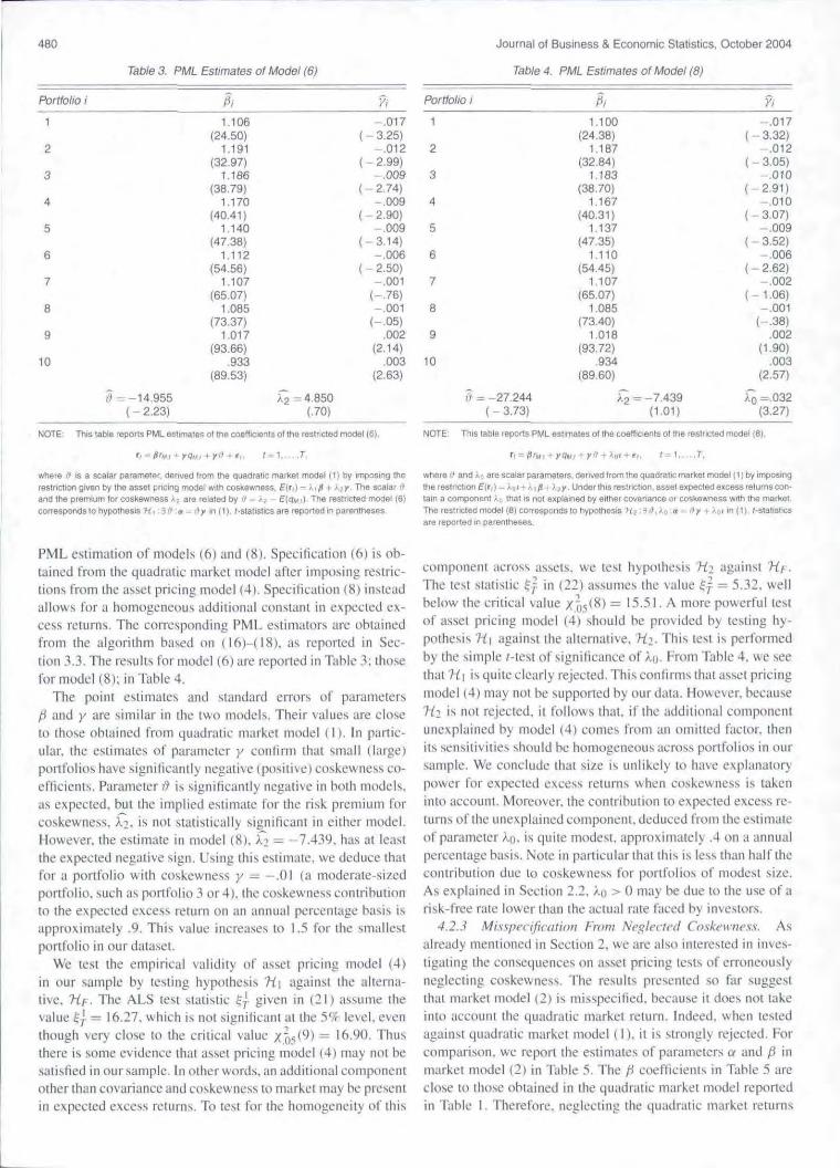
Table 3. PML Estimates of Model (6) Table 4. PML Estima tes of Model (8)

Portfolio i ii, }/; Portfo lio i ii, Yi1.106 - .017 1.100 - .0 17

(24.50) ( - 3.2 5) (24.38) (-3.32)2 1.191 -.0 12 2 1.187 - .0 12

(32.97) ( -2.99) (32.84) ( -3.05)3 1.186 - .009 3 1.183 - .0 10

(38.79) ( - 2.7 4) (38.70) ( - 2.91)4 1.170 - .009 4 1.167 - .010

(40.41) ( - 2.90) (40.31) ( - 3.07)5 1.140 - .009 5 1.137 - .009

(47 .38) ( - 3.14) (47.35) ( - 3 .52)6 1.1 12 -.006 6 1.1 10 - .006

(54.56) ( - 250) (54.45) ( - 2.62)7 1.107 - .001 7 1.107 - .002

(65.07) (-.76) (65 .07) ( - 1.06)8 1.085 - .00 1 8 1.085 - .001

(73 .37) (- .05) (73.40) (-.38)9 1.017 .002 9 1.018 .002

(9366) (2.14) (93.72) (1.90)10 .933 .003 to .934 .003

(89.53) (2.63) (89.60) (2.57)

iI =- 14.955 ;:; = 4.850 ii = - 27.244 G= - 7 .439 f,i =.032( - 2.23) (.70) ( -3.73) (1.0 1) (3.27 )

NOTE: This table reports PML estimates 01the coetticients 01the restncted model (6) ,

where r' is a scalar parame ter, denved from the quadratICmar ket model (1) by Imposrng the

restrcnon given by the asse t prICing mode l With ccskewness. E( r, ) ;: A, fJ +A.1Y, The scalar rj

and the premium lor coske wness Io. ~ are related by II = ;,2 - E(qM, j , The restricted model (6)

corresponds to hypothesis 'H, : 31"1: C/ "" l' r In {t] . r-steneucs are reported in patenmeses.

P~'1L cstirnntion of models (0) and (8) . Specification (6) is oh­rained from the quadrat ic market mod el after imposin g restr ic ­tion s from the asse t pricin g mod el (4) . Speci fica tio n (8 ) insteada llows for a homogen eou s addi tiona l constant in ex pec ted ex­ce ss returns. Th e co rrespond ing PML es tima tors arc obtainedfrom the a lgo rithm based on ( 16)--(18). as re por ted in Sec­

tion 3.3 . Th e re sult s for mod el (6) arc report ed in Tabl e 3: thosefor model tx): in Table 4.

Th e point es tima tes and standard e rro rs of param eter sfi and y are similar in the two model s. Th eir values arc closeto tho se obt ain ed from qu adrat ic market mod el ( I) . In partie­ular, the es timates of parame ter y confi rm that sma ll (la rge)port folio s have sig nifica ntly negat ive (pos itive) coskewncss co­e fficients. Param eter 1J is signiticantly negati ve in both model s.as ex pec ted. hut the implied estima te for the risk premium forco skcw ncss, f~ . is not statistically s igni fica nt in e ither mod el.However. the estima te in mod el (8). J:; = - 7,439. has at lea stthe expected negati ve sig n. Using thi s es tima te . we deduce thatfor a portfolio with coxkcwn css y = - .0 1 (a mod erate -sizedportfolio . such as portfoli o :' or 4 ). the coskewncss contri butionto the expec ted excess return on an annual percentage basis isapprox imate ly .9. Thi s value increase s to 1.5 for the sma llestportfolio in our dataset.

\\le test the empirica l valid ity of asse t prici ng model (4)in our sample hy te sting hyp oth e sis 'HI aga inst the alterna ­tive. 'HI . Th e ALS test statistic ~j. given in (2 1) assume theva lue ~j. = 16.27. wh ich is not significam at the 5lh' level. even

though ver y c lose to the cr itica l va lue X .~5( 9) = 16 .90 . Thu sthere is SOI11l' evi de nce that usse t pricin g mod el (4 ) may not besati sfied in our sample. In oth er wo rds , an addi tio na l compo nentother than covaria nce and coskcwnes s to mark et may be pre sentin expec ted excess returns. To test fo r the hom ogeneit y of thi s

NOTE: This table reports PML estima tes 01the coefficients 01the restricted mode l (8),

T/ = /Jr,,,, + r qu , + r ,1 + AUr + t ,, t =I ,. ,. T.

where /1 and An are scalar parameters. cerwed Irom lhe quadrenc marke t model (1) by Imposingthe resmcncn E( f r) = Ani + Al fl +- }.1r . Under thiSresvcuoo. asset expected excess relurns con ­tam a component AO that IS nOI explamed by either covariance or cossewness wllh the marke t

The restricted model (8) corresoooos 10hypo thesis 112 :3 IJ,Ao :a - ,~ r + Aor In (1). r-sreustceare reported In paren these s

compone nt acros s a sset s. we test hypothesis 'Hz aga inst 'Hr .TI . . ," ,

1(' rest stansnc r;;, j In (22) assume s the value ~i = 5.32. we llbelo w the cri tica l va lue X.Z)s (X) = 15.51 . A more powerful testof asset pricing mod el (4 ) should he prov ided by te sting hy­

pothe sis 'HI againsl the alt ern ati ve. 'H ~ . T his test is performedby the simple r-test of signifi cance of AO' Fro m Table 4. we seethat 'H I is qu ite clearly rejected . Thi s confirms thai asse t pr icin gmodel (4) ma y not he supported hy our data. However. becau se

H~ is not rejected. it fo llow s that. if the add itio na l co mpone ntunexpl ain ed by mod el (4) COI11l': S fro m an omi tted fac to r, thenits sensitivities should he homogen eou s ac ro ss po rtfoli os in oursample. \Ve conc lude that size is unlike ly to have explanatory

Po\VCf for e xpected ex cess ret urn s when co skcwness is takeninto account. M oreover. the contributio n to expected excess rc­turn s of the uncxplaincd component. deduced fro m the estima te

of pa ram eter AD. is quit e mo de st. approxim atel y .4 on a annualpercent age basis. No te in particul ar that th is is less than half theco ntribution du e to cos kew ncss fo r portfol ios of mod est size.As ex plained in Sec tio n 2.2. AD > 0 may be due to the use of arisk-free ra te lower than the actu al rate faced hy inve stors ,

4.2.3 lvli,\'.\pccijicatioll From Neglected Coskrwness. Asa lready ment ioned in Section 2. we arc a lso interested in invcs­tigal ing the consequences on asset pric ing tests of erroneou slynegle cting cos kcwness. Th e results present ed so far sugges tthat marke t model (2 ) is misspcci tlcd. because it docs not ta keinto account the qu adratic mark et return . Indeed . when testedaga inst qu adrat ic mark et mo de l ( I). it is strong ly rejected . Forcompa riso n. we report the estima tes of param eter s a and f3 inmark et model (2 ) in Tabl e 5 . The Ii coe ffic ients in Tah le 5 arec lose to those obt ai ned in the qu adrati c mark et model re po rtedin Tuhlc I . Th erefore. neg lec ting the qu ad rat ic market re turns

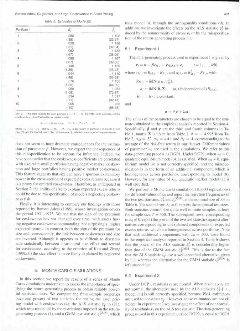
Barone Adesi, Gagliardini, and Urga : Coskewness in Asset Pricing 48 1

and

Rr ., = Rf . a ronslant.

The data-generating proce ....... u...cd in experiment I is given by

5.1 Experiment 1

1 = J. .. . . 450.r, = a + {Jr .H., + Yl/ .\I., + E,.

e, - iid:-.'(tl . 1:I. Ce, ) independent of IR,I.I ).

where rv. = R\I ., - Rf .,. and qst» = R.~, . , - RF.,. with

N,H., ..... i id ;\: (/1.H. (J,~, l.

a = iI Y + All'-

tcst .... mode l (4) through the ort hogonality con di tio ns (9). Inaddition. we investigate the effects on the A LS sta tistic ~). in -duccd by the non normality of e rror E, or by the misspcc itica-tion o f the return-generat ing procc ( I).

The value ... o f the parameters are chosen 10 he eq ual to the est i­mate s obta ined in the em pi rica l ana lys is reported in Section 4 .

Spec ifica lly. p and y are the third and fourth co lumns in Ta­ble 1. ma trix 1: is taken from Table '2. iJ = - 14 .995 fro m Ta­hle J. liM = .52. aM = 4.4 1. and R,,· = .4. corres ponding to theavcruge of the risk- fret: return in our dataset. Different valuesof parameter Ao arc used in the simulations . \Ve refer to th isdata-generat ing process as DGPI. Unde r DGPI. whe n ).0 = O.quadratic equi librium mod el (4) is sa tisfied . When i.o =F O. cqu i­Iihr ium mo del (4) is not correc tly spcc itlcd . and the misspec­ification is in the fo rm o f an additiona l co mpo nent. whic h i....homogen eous across portfo lio.... "..o rrcsponding to Illud e I (X) .However, for any va lue of ).0. quadratic ma rket mod el ( I ) iswell specified.

\Ve perform a Monte Carlo simu lation ( IO,(XX) repl ications)for different va lues of ).0 and report the rejection trequc ncie.... of

the two test vtuti...tics.~} and ~?\ IM . at the nominal size of .05 inTab le 6. The second row. i.o = O. reports the empirical tes t sizes.Hoth ... tat i-tics co ntro l size quite we ll in finite samples. at leastfor sample si/ c T = 450. The subsequcm rows. correspondingto i.o #- O. report the powerof the two test statistks again ...t alter­native ... corresponding to unexplained components in expectedexcess returns. \\ hich are hornogcncou ... across portfolios. Notethat such additional component .... with i.o=.033. were foundin the. empirical ana ly... is reported in Section 4 . Table 6 ...how-,

that the power of the ALS ... ta t i st i c ~) i... considerably higher

than that of the G~ I ~ I ... tatistic ~ .~ \I \ I . This is due to the fac tthat the A LS statistic ~l use :1 well- ...pcciticd alternative givenby ( I ). whereas the alternative for the G~ 1 ~ 1 sta tistic ~P\I !\ f isle ft unspecified,

r. I " . + #,r"" + ~ , , ' - l ....T. - l . N

Table 5. Estimates of Model (2)

docs not see m to have dram atic consequences for the cs tim..l ­

tion of param eter fL However . we ex pec t the co nse quences ofthi s mis spcc ification to he se rious for inference. Indeed . wehave see n ea rlier that the cos kcw ncss coefficie nts are corre late dwith size. with sma ll port fo lios havin g negative mark et coskew­ness and large port foli os hav ing pos itive mar ket co- kcwncvs.Thi s feature suggcsts that sill' can have a spurious explanatorypow e r in the cro ......-scction of expected excess re turns because itis a proxy for omitted coskewncss . Therefore . as anticipated inSectio n 2. the abi lity of size to explain expected excess rcturn-,cou ld he due to rn isvpccification of models neglecting co-kew­nc...s risk .

Fina lly. it is interesting to compare our findi ngs with tho ...ereponed by Barone Adcvi (ll.JX5). whose investigation coversthe period 1931 -1975 . We see tha t the sign of the premiumfor covkewncs-, has not changed over time. with aloo ...ct .... hav ­ing negative co-kcwnc...... commanding. no t surprisingly. higherexpected returns. In contrast. both the sign of the premium forsize and. con ...cqucntly, the link between covkcwncvs and sill'arc inverted . Although it appears to be difficu lt to discrimi­nate stuti... tica lly between a .... tructural si/.e effect and rewardfor co ... kcwncw. according to the cri terion of Kim and Zhang( 191.J1.Ja.h) the size effect is more like ly explained by neglectedcoxkcwncsv .

Portfolio i iii /l,.080 1.102

(.39) (23.97)2 .050 1.188

(.3 1) (32.34)3 .092 1.183

(.67) (38.09)4 .088 1.167

(.67) (39.65)5 .148 1.135

(1.36) (46.43)6 .044 1.110

(.48) (53.69)7 .076 1.105

(1.00) (64 .39)8 .069 1.083

(1.05) (72.67)9 .034 1.017

(.71) (92.41)10 .005 .933

(.10) (88.18)

NOTE Th.s table repons for each portfolio I. j ", 1. 10 the PML- SUR astmates ollhecoetf!Cl8nts" fl, of the tradlltooal markEl l model

where r" R I R, , and ril l R"" R" . R.j IS the return 01 portfolio. lI'I month I . andR.. , (R, , I .s the marke t return Ithe nsk-tree return) . /·s tatISUCs are reported In paren theses

5. MONTE CARLO SIMULATIONS

In thi ......cc tio n we repo rt the res ults of a seri c ... of Mont eCa rlo simulations undert aken to assess the importance of spec­ifyi ng the ret urn -gen erat ing process to ob ta in reli ab ly power­ful stm io,;,\ical test s. We compare the finite -sample propcni c ...(loo i/e and power ) o f two statistics for testin g the asset pric­ing model with coskcwness (4) : Ihe ALS s lat ist ie ~) in (2 1).

whic h lests mmiel (4) hy thc restr iction s imposed on thc relurn­genl'rating prore ...... ( I ). and a G MM tes t sta tistic ~Y i\ l \l. which

5.2 Experiment 2

Unde r DGPI. residu als £1 arc no rma l. Wh en re sidual s e, arcnot norma l. the alte rna tive used hy the ALS stat is t ics~} [i .e ..model ( 1)1 is still correc tly ....pccifico . becau se P~1L estimatorsarc used to co nstruc t ~} . However, the se es tima tors are not ef­licient. In e xperiment 2 \\'e invcs tigatc the e ffec t of nonnormal ·ity of re....idu al s € , on the AL S test stati.... lic. Th e data-generatingproccss lIscd in thi s ex pe rime nt. ca lled DGP2. is cq ua l to DGPI

482 Journal of Business & Economic Statistics , October 2004

Table 6. Rejection Frequencies in Experiment 1 Tetxe 8. Rejection Frequencies in Expe riment 3

o.03.06.10.15

.0404

.0505

.0712

.12 17

.2307

.0559

.4641

.9746

.9924

.9945

o.03.06.10

~ f unde r DGP4(homoscedasticity)

.0587

.3683

.9333

.9855

~ + under OGP3(conditional neterosceossticity)

.0539

.1720

.5791

.9373

NOTE This table reports the rerecton l requer'l(:l9S of the GMM stansnce ~F" [derived NOTE' This table reports Ihe rejection frequencies al lhe ALS statlstlCs ~ ; [In {2111 1or test-from {gIl and Ihe AlS steusucs tl lin (21)) for lestlng the asset pricing model with ccskew- '"9 (41.ness (4 ),

at Ihe .05 con fidence level , In axpenrnantt , The dala-generallng process (called DGP1 ) used in

thIs exper iment IS given by

I, : a + {J r"" + yq"' r+ If j . 1=1 , .. , 450.

at the .05 con fidence level . in excerereot 3. In this expenment we ccosoar tWOda la -gen eratlng

proc ess es (called DGP3 and DGP4j haVing the same uoccnononer vene nce 01 the resKluals F, .

bur sucn thaI the res iduals ,I , are conditionally neteresceoasuc In one case and rorrosceesstcin the other case. Spec ifica lly. DGP3 IS the same as DGP1 (see Table 6). buf the encvenone ,I ,

toncwa conditIOnally normal. multrvartate ARCH{I ) process Without cross-enects.

where rw r = R"u - R~ .I and q.." '" Rt" - R, ,. With

6, .... iidN(O.l:), (. r) Independenl 01(R.",) ,

R",r = R" a constant.

">d

The metro Sl = [w,l;s chosen as in Table 2. and (I "" .2. DGP4 is Similar to DGP 1 (eee Table 6) .Wllh lid r ormarmnovanons whose unconditiona l vanancemetnx IS the same as the unco ndition alvariance 01,1, in DGP3 Thus unde r DGP 4.lhe anernatwe of the Al S erauarcs ISwe lt speci fied .but not under DGP3

a = r~y + Aa·

Table 7. Rejection Frequencies in Experiment 2

i =j

i i'j.

In this artic le we have considered market coskewness andinvestigated its implications for testing asset pricing models. Byestima ting a quadratic market model. which includes the marketreturns and the square of the market returns as the two factors.we showed that port folios of smal l (large) firms have nega tive(positive) cos kcwncss with market return s. Th is find ing impli esthat small firm portfolios are exposed to a source of risk (i.e..market cos kewness) that is different from the usual market betaand arises from negative cova riance with large absolute marketreturn s. We have show n that the cos kewness coefficients o f theportfolios in our sample are statistica lly significant. This findingrejects the usual market model and demonstrates the validity ofthe quadratic market mode l as a possible exte nsion .

The ana lys is of the premium in expected excess returns in­duced by market co skewness requ ires the spec ification of ap­propriate asset pricing models including co skewness among the

heteroscedasticity of errors e .. \Ve thus consider two data­generating processes having the same unconditional varianceof the residuals e.. but so that the residuals E , are conditionallyhetcrc scedustic in one case and hornoscedastic in the other case .Spec ifica lly, DGP3 is the same as DGPl, but innova tions 8 1

follow a cond itionally norm al. multivariate ARCH ( I) processwithout cross-effects.

6. CONCLUSIONS

Matrix Q = l<Vij l is chosen as in Table 2. and p = .2. DGP4is similar to DGP I, with iid normal innovations with the sameunconditio nal variance matri x <.IS innovations 8 , in DGP3. Thu sunde r DGP4. but not under DGP J . the alternative of the ALSstatistic is well specified. The rejection frequ encies of the ALSstatistic under DGP J and DGP4 arc reported in Table 8. Th emisspeciti cation in the form of co nditional heteroscedasticityhas no effect on the em pirica l size of the statistics in these sim­ulations. The power of the ALS test statistic is reduced . but notdrastically.

.0617

.3781

.9368

.9876

.9910

o.03.06.10.15

NOTE : Th is lable reports me rejection t-eqceoces 01 the Al Sstatistics ( ; [in (21 )] lor lestlng (4) .

atme .05 conuc eoce level . in espanment 2. The data-generatingproc ess use d In this experim en t (called DGP2) IS me same asDGP 1 (see Table 6). bul the rescuers F, lollow a mulflvariate' · dlsl rrbulion w~h 5 degrees 01 treedom, and a correlat ion matnxsuch that the variance of ,I , is the sama as under DGP1 .

5.3 Experiment 3

In the Mon te Ca rlo exper iments co nducted so far. the al­ternative used by the ALS statistic was well specified. In thislast experiment. we investigate the effect of a misspecifica­tion in the alterna tive hypothesis in the form of conditiona l

but residuals E , follow a multi variate I-distrihution with 5 de­grees of freedom . The correlation matrix is chosen so thatthe resulting variance of residuals E, is the same as underDGP I. The rejection frequencies of this Monte Ca rlo simula­tion ( 10.000 replications) for the ALS statistic ~j. are reportedin Tahle 7. The ALS sta tistic appears to be only slightly over­sized . As expec ted. power is reduced compared with the case ofnorm ality, However. the loss of power caused by nonnonnalit yis limited . These results suggest that the ALS statistic does notsuffer undul y from nonnorm al ity of the residuals.

Param eters fJ and yare the tturd and fOUfth co lumns in Table 1. the matnx r IS taken Irom

Table 2. r'::z - 14,995 from Table 3. /1", = .52. 0., '" 4 ,41, and R, = .4. correspond ing to theaver age 01the ns~Aree return In our datase t. Under DGP1. when AC_ O. the quadra tICequilib­

rium mod el (4) is sansfied . When AC * O. the equi libr ilJmmodel (4) ISnot correctly specrhed . andthe rmsspecdic auon IS In Ihe term of an additional component homogeneous across portfolios.

co rresponding 10 model (8) .

l

Barone Adesi. Gagliardini, and Urga: Coskewness in Asset Pricing

rewarded factors. To obta in testi ng method ologies that are morepowerfu l than a GMM approac h. we tested asse t pr icin g mod e lsincluding coskewness through the restrict ions that they imposeon the qu ad rat ic mark e t mod e l. We used asy mpto tic test sta ­tist ic s whos e finite-sample properti es arc valida ted by mean sof a series of Monte Ca rlo simulations. \\'e found ev ide nce ofa component in expected excess returns that is not explainedby eithe r covariance or coskewness with the mark et. However.this unexpla ined co mponent is re latively small and is consis te ntfor ins tance wi th a min or rnisspe ci ficati on of the ris k-free rate .More imp ortan t. the unexplained co mponent is ho mog e neo usac ros s portfol ios. Th is find ing implies that add itional var iables.rcpresc ruing portfoli os c harac teristics suc h as firm size. have noexplanatory power for expected excess return s once coskewnessis taken into account.

Finall y. the homogeneity property of the unexp lained cornpo­nent in expected excess returns is not sa tisfied whe n coskcwncssis neglected. Th e re fore . our resul ts have impo rtant implicat ionsfor test ing methodologies. show ing that neglect ing covkcw nc-srisk ca n ca use mis leadi ng inference . Indeed. becaus e coskew­ness is positive ly corre lated with size. a possib le j ustificat ion forthe anomalous explanatory power of size in the cross-secti on ofexpected returns is that it is a pro xy for omitted coskcw ncssrisk . Th is view is supported by the fact that the sign of the pre ­mium for coskcwncss, contrary to that of size. has no t c hange din a very long tim e.

ACKNOWLEDGMENTS

The authors thank the participants in the 91h Conferenceon Panel Data. the 10th Annual Co nfe rence of the EuropeanFina ncial Management Associ ation. the Co nference on Mul­timoment Cap ital Asset Pricin g Model s and Re lated Topics.the Ii>:QUIRE UK I-lth Annual Seminar on Beyond Mean­Variance: Do Higher Moments Mauer? the 20()~ ASSAMeeting, and P. Balestra. S. Cain -Polli , J. Chen. C. R. Han ey.R. Jagannathan, R. Morek, M. Roc kinger, T. Wansbcck.C. Zh ang. two ano ny mo us referees. and the ed itor. Eric Ghysels,All of them have co ntributed. th rou gh di scussion. very help­ful comments and suggestions that im proved th is article . Theusual di scl aimer applies. Th anh are also du e to K. Frenc h.R. Jagannath an, and R. Kan for provid ing their dataset . S"' i s~

i>:CCR Finrisk is gratefully acknowledged by the tiN twoaut ho rs.

APPENDI X A: RELATIONSHIP BETWEENCROSS-MOMENT COSKEWNESS AND

THE Yi PARAMETER

In thi s append ix we show ho w the paramete r Yi rel ates tothe cox kcwncs s te rm of our quadratic market model. \Ve a lsorep ort erro r es timates whe n the cross-mome nt cos kewncs s isap prox imated by the param eter Yi.

Our basic model is [see ( 1)1

ru = Ui + fi,( RJ/,t - RF.,) + Yi ( R~1.t - Hr .,) + £ ;, t .

where

483

The probab ilistic measure of coskewness is de fined by

covl r" i. R~I . , ) = Elru R;, ) - El r,,;IEIR;,) .

which can be rewritt en as

cov(r,.i. R~f ,,) = fI,(E[ R{r.rI - E[ R~r.r IE[R,I( . t1 )

+ Yi s'arlR~/.I1 + EIR.;/.IIE[f,t1 .

In the final eq uation . the first te rm is a measure of the mar­ket asy mme try. the second term is essentially our measureof cos kewness. and the final term is equal to 0 by ass ump ­tion ( I()). Evidently. our approach considers the second termonly. However. our claim is motivated by the negligihle effectsof the fi rst term. In fact. for values fI, = I and Y, = -.0 1.whichare represe ntat ive for sma ll firm port foli os. the first term is . 1.whereas the second is - 15. If Yi is equa l to .003. as in largefirm portfo lios. then the terms are eq ual to . 1 and ~ . Fina lly. ifthe port folio has a Yi = O. then the second term is also O.

\\'e are greatly indebted to one of the referees. wh ose com­ments highlighted this point.

APPENDIX B: PSEUDO-MAXIMUM LIKELI HOODIN MODEL (8)

1n this append ix we cons ider the P~1L estimator of model (8 ).

defined by maximization of (15). We lirst derive the PML equa­tions. Th e sco re vector is g iven by

TaLl " - I

a«r .y' )' = L... II, e r e..t=1

T__ ,_~I...:_T'----- L -, - I= Z:!: e..aW. ),n)'1=1

and

aL, I T _ _ [~ ' ]-:"::":'_=-:;P :!: I ® :!: I" sech L...("' , -:!: ) .~ vcc ht E ) _

'=1

where lit = (r.\I .l .q.\I ., + a )'. £ , = r, - fl rM., - yq.\I ,1 ­y tJ - ).0 1. Z = (y. n. and I' is such that vec(:!:) = P vechfE ).By equating the score to O. we immediately find ( 16)-( I8) .

\Ve now deri ve the asy mpto tic d istributi on of the P~lL es ti­mator in mod el (8). Unde r usual regul arit y co nditions (se c the

re ferences in the main text) . the asympto tic d istri bution of thegeneral P~IL estimator ii defined in I I I) is given by

"fil ii - 0° ) .i... NIO. .Io110.10I).

whereL, (the so-called " informa tion matrix" ) and 10 are sym­metri c . positive-definite matrices defined by

. [ I i)2Lr 0].10 = hm E -- - -, (0 )

T~", T iJOaoand

[I ilL7 ilLT ]10 = lim E __(0°) __, (0° ) .

7 - 00 T iJO ilO

464 Journal 01Bus iness & Economic Statistics. October 2004

\\'e now compute matriccsJn and 10 in model (8) . The seco ndderi vatives o f the p...cu do- log- like lihood are g rvcn by

l ' L T,. I = - "' II,II ' 0 r - l .

il (/f . y ' )' il (/f. y ' ) :':I '

Th e asymptot ic va riance-covariance or(p'.y ' )' an d (;:j . ~) '

is given ex plic itly in block fo rm hy

[ '.11 " I ~ J, ,,, - I _ • 0 • (J

• 11 - , . 1 1 , "'11 .• 0 . 0

.~., t. , T,-./ =- "' 1I0 r - ' z.

~( R ' ' )" ' «(}' )' L 'f p . y u • An 1= 1

and

.I~ ' I = tr r+ H 'I -1 0 r

+ Ir, IH '( r r + H 'I- 110 z(z'r - IZ j- IZ'.

.I ~ ' ~ = - r, lA0 z<z'r - IZI- I.

, ,,,11 _ , *11'• () - . 0 .

with the other ones vuni... hing in expectation. It follows (halma­trices .lo and 10 ere g iven by [in the block repre sentation co rre ­sponding to (fl' . v ' , O. AO) ' and vccht E j]

_-,-=:-i1=L~1-:-:::-c = ~ I' / r - I 0 r - ' I';h ech( r ) iI vec ht r )' 0

- ~ l'l r -' 0 r - I (tE'E;)r- ' I'I= J

- ~ I'l r -' (tE'E;)r - ' 0 r - II'.1= 1

, [ .I (~, 0 =

\\.. here

and [.I (~ "S] o ]10 = .... I I .... - •

.loS 'I .IoKlo

and

J~~~ = t I + A'r, 1A)(Z'r - 1Zl- I.

Finally. we consider the asymptotic d istribution of es timato r

i defin ed in ( 19). T he est ima to r

I

- I '"p. = T L f,.1= 1

where f, = (rA/ ,I' l/.\1.l) " call be seen as a co mponcm ofthc P~lL

cstirnator o n the ex tende d pscudolikclihood

Lrt H. p. rd

TI T= Lr tH) - " log del r,. - :;LII',- IL)'r , 1(I', - p ).

.. .. /=1

where 1.1' (H) is g iven in ( 15). It is eas ily seen that H an d ilL. l:r>are asy mptotically ind ep endent . It fo llows that

\ I"I ./Tt r:~ - i. ~.o)1 = Er. ~ ~ + V"I ./T(1j - ,9011.

and lin the block form corresponding to (P'. y ' )' . (d. i .n) ' 1

(All parameters are eva luated at true va lue) , Th erefore. the <1"'­ym pto tic var iance-covariance ma trix of the P7\IL est imator '9 inmodel (8) is given by

APPENDIX C: ASYMPTOTIC LEAST SQUARES

In thi ... appendix we de rive the t\LS ...ta t i... ti c ~} in (2 1) an d~i in C~2) . In bot h case ... the restric tions [see (20)1 are of the

form

The text .... tat ist ics fo llow.It sho uld be no ted that exact te sts (unde r no rmality ) ca n be

co nstruc ted for test ing hyp oth e se s H 1 and "H. '2 agai nst 'Hf" (sec.c .g .. Zhou 1995: Vclu and Z ho u 1999 ). Th e se tcsb arc asy m p­toti call y equ iva lent to the ALS te sts used in th is artic le for the irco mputatio nal sim plici ty. An evaluation of the tin itc-sample

properties of the ALS test sta tistics is presented in Section 5.

~IH .;o 1 =A, (a) vectll ) + A ~ (a l .

where II is the N x 3 ma trix defined hy II = la P y I and,\ 1(a) i-, ...uch that

Ada ) = (I. O. -() ) 0 Iv " Ai l" l 0 1.-..

\Ve derive the we igh ting matrix So = (f)g /ilH' Qu ilg / ilO)- I.

where 120 = 1',,( fi lii - H ) ). From (131, we ge t

a" il u' .-~ Q -~- = A'EI F F' I - I A' 0 r110 ' 0 iJO I I , 1

= I I + A'rJ- 'A)r .J~- l QS] .

K

i. 0 r - IZ]z'r - Iz

[i. 0 r - ' ]

q = z'r - I .

S = covls .. \'l~ch{ e{E;)l

K = \arl\echI E,E;i1.

.I, _ [ EIII ,II ,10 r - I0 - i: Z' 0 r -1

and

Note that the a ...ymptotic variance-covaria nce of (fi '. y'. ;:j. j~) '

( i.e .. .J l~ - l ) doc s not dep end o n the di stribut io n of erro r term

e ., and in parti cul ar it coincides with the asympto tic vuriuncc-.covariance matrix o f the f\lL estimator of (ii'.y '. ~ . ~» '.

when £ 1 is normal. In contrast. asymmetries and kurtovisof the di stribution of e, influ en ce the asymptotic va riance­

covariance matri x of "cch(!: ) and the as ymptotic co varianceof (fi '.9'.7i. j~) ' and vcch t I:). throu gh matrices S and K .

Barone Adesi, Gaqliardmi. and Urga : Coskewnes s in As set Pricing

REFERENCES

Bane . R. W. ( l lJ~ll . "The Relation..hip Bet ....ccn Return and \1ar~el valueti l"Common Stock s," Jf/I/ m al of rinancialEconomirv . lJ. J.. I X.

Barone Adesi. G. (l lJX5). "Arhma~c: Equilib rium With Skc.... cd :\ ..-.("1 Retu rn...:'Jfllmldl (1Financial tim! (Jlltmtittlf ;,,· Analvsis, 20. 2W-J 1.1.

Barune Adc..i. G .. and 'Iulwur. r. ( IYlSJ). " \br~ct \li)(],:l.. an d It....tcro-ceda ..tic ­it) of Residual Security Returns." Journal fif Hu\ in(' .\.\' ..( ECll llomic !>1t1/i_\lin .

I. 16.\ -1 610\.BJad. E ( l lJnl. "Capita l ~1J.f~et Equ ilibrium with Rc..meted Borrowin g,"

luurna! of UII_\i/le_l.\. ~5 . -1-1.+-1 55.Bolla,..k·\ . T.. and Woo ldrid !!l\ J. ,\I. I J9iJl ). ··() u<J ..i- ,\J,J\ imu llJ l.iJ..dihoou

Ecrim.uion and Inference in Dynamic Mude h With Time-varying Covari ­ancc s," Econometr«: R/ 'I 'i/ 'I~I , I I. 1~3-1 72 ,

Breede n. D. T. ( 1979 1. "A n lnwncmporal I\..:..<.· t Prici ng Mod el with Sto­cha ..tic Co nsumption and 111n: ..rmcnt Oppon unitic..:· Journ af /1 f"imll/ dal!;·n momic.\" . 7. 265 - 290 .

Call1phdi. J . Y.. Lo. A . W.. and Mal·Kinlay. A. C.119K71. The LnJllo!l/t'lr;n 01Financial ,\!l/ r l.:.t'I.\. Princeton. NJ : Pr inceton Uni, er~i l ) Pre.....

Chamberlain. G .. and Ruth ..child. ~ 1. ( 14S31. "Arbitrage. l-actor Struc tureand ~lean variance r\n;II~ ..i-, in Large A"'I.'I ~1ar~..:" : · Econometrica. 5 1.

1 2~ 1 - 130 1.

Dittmar. R. F. (200 ::!l. "Nonlinear Pricin g Kcrrcl -. Kuno..i.. Pre ferenc e . an db iden cc From lhe Cro....- S~..("l illn of Equit~ RelUrm : ' JOlln w l of F;mlfl Ct'.

57 . ,1hK-40 3.Engk· . R. F..lJend!1.lJ. F.. and Ril·hard. J . E j IlJSXI."E \. II~ l·nl.' i l ~ : · r;O I1lt/lII t'l ­

rinl. 51 . 277- .104.F.I111a. E.. and h en eh. K. R. IIIN5 1. "S i...e a nd Bi'llI~ -tn..\1arJ..cl Fa..:lor.. in Earn ­

ing" and Return..... JOllnw / lif Filllma. 50 .131 -1 55 .fi uuri erou\.. C . and Ja ..i;IJ... J . (200 11. FinO/will i t 'n momt'lri n . Prin n 't lln . 1'\J:

Prinl'ehln Uni\ er~ i l ) Pre.....Guurier<lu,( , c.. \ Ionfon. A .. anu Trognun. A. ( l lJX~1. " P....:udc}..\1a\.imum

l .i ~c l ihi ll ll.l i\1I.'1hcllh; Them )': ' /;"n mlllllt·lrit ·ll. 52. 6XI- 7(MI.___ ( IIJS5 ), " i\1o inJ rl.''' Clrrr.. As)'mplOlique ..:· Ali/wit's dt' f' I,VSI;,/;". 58,

t) I -I n .lI a ll'ol·l1. I.. P, ( 19X21. " I.arge- Sample Pro peni c.. of Gelll'rali/l'd I\kthod -uf­

MOllll' nh E..tirnalor..:· f nmflllll'tr;m . 50 . 102q- I05~ .

Ib n..en . 1.. P.. and J<lganllalhml, R. ( llJY7)...A.....e....ing Sp<.·cili calioll Erwr.. inSII-...:ha..lk Discuunl !-"<lelor \1 ode b : ' Jlllin/(/ l of FiI1tl/I ('('. 52, 557- 5'Xl.

Harve)'. C. R.. and Siddi4ue. A. (10110 ). "Cond itional S~cwne .... in A..\I.'\ PriL'ingiC~h." Jill/nUll /1 fimmn'. 55. 1:!:6.1-lllJ5 ,

485

J.If!:lOnarha n. fL <JnJ wan g. Z. ( 199M. "Ttk· Con d i/i(ln<J1 C /\ P.\ l.md Ihe Crt l .... ­

Section of Expected Rerum....· Jf/llnw l of t inance . 5 1. .1-5.1 ,___ (2(X)11."Empirica l Evaluamm Il l' :\ ,,\I.'t Pricing \ltll,k h: :\ Compa ri..on

of the SI>I' and Bet a \klhlld ..: · wurking paper. Xort hwc..tern L'nh cr..i t~ .

Kun. R.. and Zhanc. C. 1IlJiJlJ,1I. "( i \ l \ l Tc..t of Stui,:hil..tic Di..count Fac­lor ~hllJcI .. \\ilh~ Ucclc.... I-actor..... Iou rna l of f imm l";a l /;"n",,,,,,in . 5~.

10.' -1 17.___ 1Il)l)l)h I...Two-Pa....Tl' ''''' ul A"\I.'I Pricmg \lillJl·l.. With l ' -ck .... I-.IC­

tor s." l oumal of ' "iI/I/1IIl'. 5~. 10J-:!.\5 .Kan . R.. a nd Zhou . G , 119iNI. "A Critique (II' the SIHc h" ..tic I>i..couru I ac tor

~kthlllJ lllllgy:' JfllInwl ' ~1 [inuncv, 5~, 1221 -l l~x .

Kraus. A.. and Litzenberger. R t 197(, ). "Skcwnc.... Preference- allJ the Valua­tion ul Ri..k A....ets," JtllImal tlf tinancv. .1I . IOS5 ~ I ItM) .

Lin tner, J. ( 19f15), "The Valua tion III Ri..k A....cr.. and the Se lection Ill' Ri..~ylnvestmcm-, in Stock Pontolio- and Capital Budge:t-.: · Hl'I";,'lr f!/ f ClllwlIlinti ll/ I SI'I/I\lin'. ~ 7. 13- .'1.

~I<.'rll1n , R. C. 11(73 ). "An Irucn cm p oral Cupuul A..~c t l'r icing Mlll.kl."l~n'I/I "'ll'l r;( '(/ . ~ I . Kh7-K K7.

S e\l,....~. W. K.• and We..t . K. D. 114X91. "A Simple PIl..itivc Semi Detin ue.Hcrc ro..ccda..ncir v and Autocorrelation-Con ..i..tent Cov .mancc \ Ial ri \.: ·f n ll/l 'fIlt·trica. 55. 703-7UK.

Ra m....:~ . J. B. ( 1%91. "Te-te for Spec ificat ion Erro re in C1<l....i.:a l LinearLeu..t Square.. Repre ....ion ,\n.il~ ..i....· Jf'lIn/ll I / ~' the Rf/ w l .\tll ti l til 'l/ I Sodt'I_\ .

Scr. B. .11. .' 50---37 1.Rn..... S . A . ( l lJ7fll. "Arhilrag~' Thc.'IIf)- of Ca pital :\ ....e:1 Pr ic ing: ' Joum ll l oj

L (·mromic TI'~'(Jn. 1.1 . .1~ l - .1hll.Ruhin..tl·in. \1 . E. i197.1). "A (\ lrnr .lr:ltit c Stalle.. :\ na l ~ ..i .. of Ri..~ Pr..:miurn: ·

Tlu' JII /m w l of H/Hill t'.n . ~h. h05--6 15 .Sha nke n. J. ( IYQ:!:). "On the: E..limaliu n of Bela Pricin g \1 0,.1..:1..:' Rl'l ii 'll of

!'i,1ll1W;Cl I S/m!il '.\ . 5. l - J J .Sharpe, \\', F. (IYh·H . "Carital A....l.'t Pri~''': '' : A TIIl'ul) til M,cr~t·t E-lJu ilihrium

Unde:r Cl1ndilil1n~ Ilf Ri,J..: · Jl!lImtl l , ~r f'i,Wfl l"l' . ~U. II XlJ- 119t1.Vl·lu . R.. and Zh~lU . G . ( 19 YYI. "TC''' ling J\.1ulli-Ikta A ....I.'I Prici ng ~te llJd,: '

JOllmaf ol Em,'irinll Filllllln'. 6. 2 1 i)-2~ I ,

While . I t ( IllS I J. ''j\ I,I\ ilttUIII l.iJ..dihclCIl.1 E..ciuMrilll1 01" ,\ Ii,,~ pt·~· i ' i l'd M, lI.1d~ ."

/; 'f"( >IIOlll i ' f rinl , 50. 1- 25.

Zellncr. A. (1962 ). "An Eflici e: nl ~klhod of btilllillillg SCl'min gly UnrelaledRl.'gre, ..ion .. and Tc .." for Aggr ....gatiu ll Bia..:· JfIIl/ m ll 01/111' "''''t 'lk lm S/tl­li lt;('(// ..\' lIodll1i ll ll . 57 • .1~K-.1hS .

Zhou . G, (1945 1. "S l11a ll-Sa lllpll.' Rall~ Te..l.. With App lieali illl" III ;\....e tPrici ng: ' JII/m /al of Elllfl i r ;f'(/l Fi l1l11we. 2. 71-lJ.\ ,

Copyright of Journal of Business & Economic Statistics is the property of AmericanStatistical Association and its content may not be copied or emailed to multiple sites orposted to a listserv without the copyright holder's express written permission.However, users may print, download, or email articles for individual use.