essays in investor behavior and asset pricing

Essays in Investor Behavior and Asset Pricing

Li An

Submitted in partial fulfillment of the

requirements for the degree

of Doctor of Philosophy

in the Graduate School of Arts and Sciences

COLUMBIA UNIVERSITY

2014

© 2014

Li An

All Rights Reserved

ABSTRACT

Essays in Investor Behavior and Asset Pricing

Li An

This dissertation consists of three essays on investor behavior and asset pricing.

In the first chapter, I investigate the asset pricing implications of a newly-documented

refinement of the disposition effect, characterized by investors being more likely to sell a

security when the magnitude of their gains or losses on it increases. Motivated by behavioral

evidence found among individual traders, I focus on the pricing implications of such behavior

in this chapter. I find that stocks with both large unrealized gains and large unrealized losses,

aggregated across investors, outperform others in the following month (monthly alpha = 0.5-

1%, Sharpe ratio = 1.6). This supports the conjecture that these stocks experience higher

selling pressure, leading to lower current prices and higher future returns. This effect cannot

be explained by momentum, reversal, volatility, or other known return predictors, and it also

subsumes the previously-documented capital gains overhang effect. Moreover, my findings

dispute the view that the disposition effect drives momentum; by isolating the disposition

effect from gains versus that from losses, I find the loss side has a return prediction opposite

to momentum. Overall, this study provides new evidence that investors’ tendencies can

aggregate to affect equilibrium price dynamics; it also challenges the current understanding

of the disposition effect and sheds light on the pattern, source, and pricing implications of

this behavior.

The second chapter extends the study of the V-shaped disposition effect - the tendency to

sell relatively big winners and big losers - to the trading behavior of mutual fund managers.

We find that a 1% increase in the magnitude of unrealized gains (losses) is associated with

a 4.2% (1.6%) higher probability of selling. We link this trading behavior to equilibrium

price dynamics by constructing unrealized gains and losses measures directly from mutual

fund holdings. (In comparison, measures for unrealized gains and losses in chapter one

are approximated by past prices and trading volumes.) We find that, consistent with the

relative magnitude found in the selling behavior regressions, a 1% increase in the magnitude

of gain (loss) overhang predicts a 1.4 (.9) bp increase in future one-month returns. A trading

strategy based on this effect can generate a monthly return of 0.5% controlling common

return predictors, and the Sharpe ratio is around 1.4. An overhang variable capturing the

V-shaped disposition effect strongly dominates the monotonic capital gains overhang measure

of previous literature in predictive return regressions. Funds with higher turnover, shorter

holding period, higher expense ratios, and higher management fees are significantly more

likely to manifest a V-shaped disposition effect.

The third chapter studies how the recourse feature of mortgage loan has impact on bor-

rowers’ strategic default incentives and on mortgage bond market. It provides a theoretical

model which builds on the structural credit risk framework by Leland (1994), and explicitly

analyzes borrowers’ strategic default incentives under different foreclosure laws. The key

results are, while possible recourse makes the payoff in strategic default less attractive, it

helps deter strategic default when house price goes down. I also examine the case when cash

flow problems interact with default incentives and show that recourse can help reduce default

incentives, make debt value immune to liquidity shock, and has little impact on house equity

value.

Table of Contents

List of Figures iv

Acknowledgements v

1 Asset Pricing When Traders Sell Extreme Winners and Losers 1

1.1 Introduction . . . . . . . . . . . . . . . . . . . . . . . . . . . . . . . . . . . . 2

1.2 Data and Key Variables . . . . . . . . . . . . . . . . . . . . . . . . . . . . . 8

1.2.1 Stock Samples and Filters . . . . . . . . . . . . . . . . . . . . . . . . 8

1.2.2 Gains, Losses, and the V-shaped Selling Propensity . . . . . . . . . . 8

1.2.3 Other Control Variables . . . . . . . . . . . . . . . . . . . . . . . . . 11

1.3 Empirical Setup and Results . . . . . . . . . . . . . . . . . . . . . . . . . . . 12

1.3.1 Sorted Portfolios . . . . . . . . . . . . . . . . . . . . . . . . . . . . . 13

1.3.2 Fama-Macbeth Regression Analysis . . . . . . . . . . . . . . . . . . . 16

1.4 The Source of the V-shaped Disposition Effect and Cross-sectional Analysis . 23

1.4.1 The Source of the V-shaped Disposition Effect . . . . . . . . . . . . . 24

1.4.2 Subsample Analysis: the Impact of Speculativeness . . . . . . . . . . 26

1.5 Time-series Variation: the Impact of Capital Gains Tax . . . . . . . . . . . . 28

1.6 The Disposition Effect and Momentum . . . . . . . . . . . . . . . . . . . . . 30

1.7 Conclusions . . . . . . . . . . . . . . . . . . . . . . . . . . . . . . . . . . . . 32

i

2 V-Shaped Disposition: Mutual Fund Trading Behavior and Price Effects 44

2.1 Introduction . . . . . . . . . . . . . . . . . . . . . . . . . . . . . . . . . . . . 45

2.2 Data description . . . . . . . . . . . . . . . . . . . . . . . . . . . . . . . . . 50

2.3 Specification . . . . . . . . . . . . . . . . . . . . . . . . . . . . . . . . . . . . 51

2.3.1 Trading Behavior . . . . . . . . . . . . . . . . . . . . . . . . . . . . . 51

2.3.2 Price Effect . . . . . . . . . . . . . . . . . . . . . . . . . . . . . . . . 53

2.3.3 Alternative Measures . . . . . . . . . . . . . . . . . . . . . . . . . . . 57

2.4 Results . . . . . . . . . . . . . . . . . . . . . . . . . . . . . . . . . . . . . . 59

2.4.1 Trading Behavior . . . . . . . . . . . . . . . . . . . . . . . . . . . . . 59

2.4.2 Pricing Effect . . . . . . . . . . . . . . . . . . . . . . . . . . . . . . . 60

2.4.3 Alternative Measures . . . . . . . . . . . . . . . . . . . . . . . . . . . 63

2.5 Exploring the link: how heterogeneity in mutual funds’ behavior affects price

patterns . . . . . . . . . . . . . . . . . . . . . . . . . . . . . . . . . . . . . . 64

2.6 Robustness checks . . . . . . . . . . . . . . . . . . . . . . . . . . . . . . . . . 67

2.6.1 Extreme Rank Dependency . . . . . . . . . . . . . . . . . . . . . . . 67

2.6.2 Simple Measures . . . . . . . . . . . . . . . . . . . . . . . . . . . . . 69

2.6.3 Placebo Test . . . . . . . . . . . . . . . . . . . . . . . . . . . . . . . 71

2.7 Conclusions . . . . . . . . . . . . . . . . . . . . . . . . . . . . . . . . . . . . 71

3 Mortgage Debt, Recourse, and Strategic Default 88

3.1 Introduction . . . . . . . . . . . . . . . . . . . . . . . . . . . . . . . . . . . . 89

3.2 Foreclosure Law across the States . . . . . . . . . . . . . . . . . . . . . . . . 92

3.3 The Baseline Model: Borrower without Cash Flow Problems . . . . . . . . . 93

3.3.1 Model Set-up . . . . . . . . . . . . . . . . . . . . . . . . . . . . . . . 93

3.3.2 Valuation and Endogenous Default Boundary . . . . . . . . . . . . . 95

ii

3.3.3 Results: Recourse, Strategic Default and Mortgage Market . . . . . . 98

3.4 Full Model: Borrower with Cash Flow Problems . . . . . . . . . . . . . . . . 105

3.4.1 Model Modification and Valuation . . . . . . . . . . . . . . . . . . . . 105

3.4.2 Results: Recourse, Liquidity Shock and Mortgage Default . . . . . . . 108

3.5 Policy Implications and Conclusions . . . . . . . . . . . . . . . . . . . . . . . 111

Bibliography 113

iii

List of Figures

1.1 V-shaped Selling Propensity in Response to Profits . . . . . . . . . . . . . . 3

1.2 Top Capital Gains Tax Rate, 1970 - 2011 . . . . . . . . . . . . . . . . . . . 29

3.1 Default Boundary, House Equity Value and Recourse. . . . . . . . . . . . . . 102

3.2 House Equity Value When House Price Falls . . . . . . . . . . . . . . . . . . 103

3.3 Debt Value When House Price Falls. . . . . . . . . . . . . . . . . . . . . . . 104

3.4 Initial Mortgage Rate, Mortgage Yield, and Recourse. . . . . . . . . . . . . . 105

3.5 Default Boundary in Presence of Liquidity Shock. . . . . . . . . . . . . . . . 109

3.6 Debt Value and Equity Value in Presence of Liquidity Shock When V=100. . 110

3.7 Debt Value and Mortgage Yield in Presence of Liquidity Shock When V=90. 111

iv

Acknowledgments

I am deeply indebted to my committee members for their guidance and encouragement

throughout the years. I am very fortunate to have had Professor Kent Daniel and Professor

Paul Tetlock as two close mentors, who led me to the fascinating field of behavioral finance

and taught me how to contribute to it. I appreciate their generous contributions of time,

ideas, and encouragement, which have helped me to grow from a consumer of knowledge

into an independent researcher. Their influence goes far beyond the inputs to my research

projects; also valuable to me are the important lessons I learned from their outstanding

scholarship. I thank Professor Joseph Stiglitz and Professor Patrick Bolton for the great

experience of working with them. In addition to their remarkable academic achievements, I

admire their efforts to bring knowledge to the broader public dialogue and their contributions

to critical policy issues of our time. I also want to thank Professor Jushan Bai for serving

as my thesis examiner.

I thank the faculty and staff at the economic department and the finance division in busi-

ness school at Columbia University. I especially thank Professor Wei Jiang, Professor Neng

Wang, Professor Gur Hurberman, Professor Suresh Sundaresan, Professor Robert Hodrick,

Professor Barnard Salanie, and Professor Tri Vi Dang for helpful discussions and guidance.

I want to thank all collaborators and colleagues that I am fortunate to have had. Special

thanks to Bronson Argyle, Laurence Wilse-Samson, and Rachel Harvey for the enjoyable

and productive collaborations. I also want to thank Fangzhou Shi, Assaf Shtauber, Andres

Liberman, Jaehyun Cho, Tao Li, Zhongjin Lv, Jia Guo, Bingxu Chen, Mattia Landoni,

Ran Huo, Qingyuan Du, Yinghua He, Adonis Antoniades, Sebastian Turban, Corinne Low,

Raul Sanchez de la Sierra, Alejo Czerwonko, Shaojun Zhang, Rui Cui, and Lei Xie. It is

impossible to name everyone, but I am very grateful to have had this great community of

v

smart and motivated people who accompanied me on my journey in pursuit of economic

science. Moreover, they have offered great friendship and shared many important moments,

whether woes of academia or the joy of a break-through.

Last but not least, I offer my deepest gratitude to my parents, An Muying and Xue

Qinsheng. They have always been a source of love, support, and strength. I also thank

Zhixing Chen, my boyfriend. I am very glad to have his company in my life. With regard

to contribution to this thesis, I especially appreciate that he understands and supports me

in tough times, that he shares the great times, and that he does laundry at all times.

vi

To my parents, An Muying and Xue Qinsheng

vii

Chapter 1

Asset Pricing When Traders Sell

Extreme Winners and Losers

Li An

2

1.1 Introduction

The disposition effect, first described by Shefrin and Statman (1985), refers to the investors’

tendency to sell securities whose prices have increased since purchase rather than those have

fallen in value. This trading behavior is well documented by evidence from both individual

investors and institutions1, across different asset markets2, and around the world3. Several

recent studies further explore the asset pricing implications of this behavioral pattern, and

propose it as the source of a few return anomalies, such as price momentum (e.g., Grinblatt

and Han (2005)). In these studies, the binary pattern of the disposition effect (a differ-

ence in selling propensity conditional on gain versus loss) is usually further modeled as a

monotonically increasing relation of investors’ selling propensity in response to past profits.

However, new evidence calls this view into question. Ben-David and Hirshleifer (2012)

examine individual investor trading data and show that investors’ selling propensity is ac-

tually a V-shaped function of past profits: selling probability increases as the magnitude of

gains or losses increases, with the gain side having a larger slope than the loss side. Figure 1.1

(Figure 2B in their paper) illustrates this relation. Notably this asymmetric V-shaped sell-

ing schedule remains consistent with the empirical regularity that investors sell more gains

than losses: since the gain side of the V is steeper than the loss side, the average selling

propensity is higher for gains than for losses. This observed V calls into question the current

understanding of how investors sell as a function of profits. Moreover, it also challenges the

1See, for example, Odean (1998) and Grinblatt and Keloharju (2001) for evidence on individual investors,Locke and Mann(2000), Shapira and Venezia (2001), and Coval and Shumway (2001) for institutional in-vestors.

2See, for example, Genesove and Mayor (2001) in housing market, Heath, Huddart, and Lang (1999) forstock options, and Camerer and Weber (1998) in experimental market.

3See Grinblatt and Keloharju (2001), Shapira and Venezia (2001), Feng and Seasholes (2005), amongothers. For a thorough survey of the disposition effect, please see the review article by Barber and Odean(2013)

3

studies on equilibrium prices and returns that assume a monotonically increasing relation

between selling propensity and profits.

Figure 1.1: V-shaped Selling Propensity in Response to Profits

Probability of selling

GainsLosses

Asymmetric probability of selling

Profits

The current study investigates the pricing implications and consequent return predictabil-

ity of this newly-documented refinement of the disposition effect. I refer to the asymmetric

V-shaped selling schedule, which Ben-David and Hirshleifer (2012) suggest to underlie the

disposition effect, as the V-shaped disposition effect. If investors sell more when they have

larger gains and losses, then stocks with BOTH larger unrealized gains and larger unrealized

losses (in absolute value) will experience higher selling pressure. This will temporarily push

down current prices and lead to higher subsequent returns when future prices revert to the

fundamental values.

To test this hypothesis, I use stock data from 1970 to 2011 and construct stock-level

measures for unrealized gains and losses. In contrast to previous studies, I isolate the effect

from gains and that from losses to recognize the pronounced kink in the investors’ selling

schedule. The results show that stocks with larger unrealized gains as well as those with

larger unrealized losses (in absolute value) indeed outperform others in the following month.

This return predictability is stronger on the gain side than on the loss side, and it is stronger

4

for gains and losses from the recent past compared with those from the distant past - both are

consistent with the trading patterns documented on the individual level. In terms of mag-

nitude, a trading strategy based on this effect generates a monthly alpha of approximately

0.5%-1%, with a Sharpe ratio as high as 1.6. This compares to the strongest evidence we

have on price pressure.

To place my findings into the context of existing research, I compare a selling propensity

measure that recognizes the V-shaped disposition effect, the V-shaped selling propensity,

with the capital gains overhang variable, which assumes a monotonically increasing selling

propensity in response to profits. Grinblatt and Han (2005) propose the latter variable,

which is also studied in subsequent research (e.g., Goetzmann and Massa (2008); Choi,

Hoyem, and Kim (2008)). A horse race between these two variables shows that once the V-

shaped selling propensity is controlled, the effect of capital gains overhang disappears. This

suggests that the V-shaped selling schedule better depicts investors’ trading pattern, and

the return predictability of capital gains overhang originates from adopting the V-shaped

selling propensity.

To gain insight into the source of the V-shaped disposition effect, I conduct tests in

cross-sectional subsamples based on institutional ownership, firm size, turnover ratio, and

stock volatility. In more speculative subsamples (stocks with lower institutional ownership,

smaller size, higher turnover, and higher volatility), the effect of unrealized gains and losses

are stronger. This finding supports the conjecture that a speculative trading motive underlies

the observed V. It is also consistent with Ben-David and Hirshleifer’s (2012) finding that

the strength of the V shape on the individual level is related to investors’ “speculative”

characteristics such as trading frequency and gender.

I also explore the time-series variation of return predictability based on the V-shaped

disposition effect. In particular, I examine the impact of capital gains tax: if investors’

5

selling behavior varies through time due to changes in tax, so should the return pattern

based on this behavior. In a high capital gains tax environment, investors are less likely

to realize their gains because they face a higher tax, but they are more likely to sell upon

losses as it helps to offset capital gains earned in other stocks. Empirical results confirm this

conjecture: compared with low tax periods, during high tax periods return predictability

from the gain side is weaker and that from the loss effect is stronger. The tax incentive has

a unique advantage as a test because it has different implications for the gain side versus

the loss side. Given the horizon of forty years in my sample, many general trends, such as

development of trading technology and an increase in overall trading volume, may result in

the V-shaped selling propensity effects changing over time; however, few have asymmetric

implications for the gain side and the loss side. This finding further validates that the

observed return patterns are indeed consequences of the V-shaped disposition effect, rather

than other mechanisms.

This paper connects to three strands of the literature. First, it contributes to the research

on investors’ trading behaviors, and more specifically how investors trade in light of past

profits and what theories explanation this behavior. While it has become an empirical

regularity that investors sell more gains than losses, most studies focus on the sign of profit

(gain or loss) rather than its size, and the full functional form remains controversial. The

V-shaped selling schedule documented by Ben-David and Hirshleifer (2012) also appears in

other studies, such as Barber and Odean (2013) and Seru, Shumway, and Stoffman (2010),

although it is not their focus. On the other side, Odean (2008) and Grinblatt and Keloharju

(2001) show a selling pattern that appears as a monotonically increasing function of past

profits. My findings at the stock level support the V-shaped selling schedule rather than

the monotonic one. A concurrent study by Hartzmark (2013) finds that investors are more

likely to sell extreme winning and extreme losing positions in their portfolio, and that this

6

behavior can lead to price effects; this is generally consistent with the V-shaped selling

schedule. The shape of the full trading schedule is important because it illuminates the

source of this behavior. Prevalent explanations for the disposition effect, either prospect

theory (Kahneman and Tversky (1979)) or realization utility (Barberis and Xiong (2009,

2012)), attribute this behavioral tendency to investors’ preference. Although these models

can explain the selling pattern partitioned by the sign of profits by generating a monotonic

relation between selling propensity and profits, reconciling the V-shaped selling schedule

in these frameworks is difficult. Instead, belief-based interpretations may come into play.

Cross-sectional subsample results point to a speculative trading motive (based on investors’

beliefs) as a general cause of this behavior. Moreover, while several interpretations based on

investors’ beliefs are consistent with the V shape on the individual level, they have different

implications for stock-level return predictability. Thus the stock-level evidence in this paper

sheds further light on which mechanisms may hold promise for explaining the V-shaped

disposition effect. Section 1.5 discusses this point in details.

Second, this study adds to the literature on the disposition effect being relevant to asset

pricing. While investor tendencies and biases are of interest on their own right, they relate to

asset pricing only when individual behaviors aggregate to affect equilibrium price dynamics.

Grinblatt and Han (2005) develop a model in which the disposition effect creates a wedge

between price and fundamental value. Predictable return patterns are generated as the

wedge converges in subsequent periods. Empirically, they construct a stock-level measure of

capital gains overhang and show that it predicts future returns and subsumes the momentum

effect. Frazzini (2006) measures capital gains overhang with mutual fund holding data and

shows that under-reaction to news caused by the disposition effect can explain post-earning

announcement drift. Goetzmann and Massa (2008) show that the disposition effect goes

beyond predicting stock returns and helps to explain volume and volatility as well. Shumway

7

and Wu (2007) find evidence in China that the disposition effect generates momentum-like

return patterns. The measures used in these studies are based on the premise that investors’

selling propensity is a monotonically increasing function of past profits. This study is the

first one to recognize the non-monotonicity when measuring stock-level selling pressure from

unrealized gains and losses and to show that it better captures the predictive return relation.

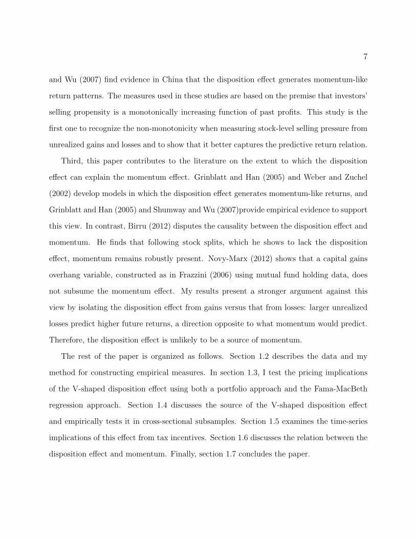
Third, this paper contributes to the literature on the extent to which the disposition

effect can explain the momentum effect. Grinblatt and Han (2005) and Weber and Zuchel

(2002) develop models in which the disposition effect generates momentum-like returns, and

Grinblatt and Han (2005) and Shumway and Wu (2007)provide empirical evidence to support

this view. In contrast, Birru (2012) disputes the causality between the disposition effect and

momentum. He finds that following stock splits, which he shows to lack the disposition

effect, momentum remains robustly present. Novy-Marx (2012) shows that a capital gains

overhang variable, constructed as in Frazzini (2006) using mutual fund holding data, does

not subsume the momentum effect. My results present a stronger argument against this

view by isolating the disposition effect from gains versus that from losses: larger unrealized

losses predict higher future returns, a direction opposite to what momentum would predict.

Therefore, the disposition effect is unlikely to be a source of momentum.

The rest of the paper is organized as follows. Section 1.2 describes the data and my

method for constructing empirical measures. In section 1.3, I test the pricing implications

of the V-shaped disposition effect using both a portfolio approach and the Fama-MacBeth

regression approach. Section 1.4 discusses the source of the V-shaped disposition effect

and empirically tests it in cross-sectional subsamples. Section 1.5 examines the time-series

implications of this effect from tax incentives. Section 1.6 discusses the relation between the

disposition effect and momentum. Finally, section 1.7 concludes the paper.

8

1.2 Data and Key Variables

1.2.1 Stock Samples and Filters

I use daily and monthly stock data from CRSP. The sample covers all US common shares

(with CRSP share codes equal to 10 and 11) from January 1970 to December 2011. To avoid

the impact of the smallest and most illiquid stocks, I eliminate stocks lower than two dollars

in price at the time of portfolio formation, and I require trading activity during at least 10

days in the past month. I focus on monthly frequency when assessing how gain and loss

overhang affect future returns. My sample results in 1843236 stock-month combinations,

which is approximately 3600 stocks per month on average.

Institutional ownership data is from Thomson-Reuters Institutional Holdings (13F) Database,

and this information extends back to 1980.

1.2.2 Gains, Losses, and the V-shaped Selling Propensity

For each stock, I measure the aggregate unrealized gains and losses at each month end by

using the volume-weighted percentage deviation of the past purchase price from the current

price. The construction of variables is similar to that in Grinblatt and Han (2005), but

with the following differences: 1. instead of aggregating all past prices, I measure gains and

losses separately; 2. I use daily, rather than weekly past prices in calculations; 3. To avoid

confounding microstructure effects, both the current price and the purchase price are lagged

by 10 trading days.

Specifically, I compute the Gain Overhang (Gain) as the following:

9

Gaint =∞∑n=1

ωt−ngaint−n

gaint−n =Pt − Pt−n

Pt· 1{Pt−n≤Pt}

ωt−n =1

kVt−n

n−1∏i=1

[1− Vt−n+i]

(1.1)

where Vt−n is the turnover ratio at time t−n. The aggregate Gain Overhang is measured

as the weighted average of the percentage deviation of the purchase price from the current

price if the purchase price is lower than the current price. The weight (ωt−n) is a proxy for

the fraction of stocks purchased at day t− n without having been traded afterward.

Symmetrically, the Loss Overhang (Loss) is computed as:

Losst =∞∑n=1

ωt−nlosst−n

losst−n =Pt − Pt−n

Pt· 1{Pt−n>Pt}

ωt−n =1

kVt−n

n−1∏i=1

[1− Vt−n+i]

(1.2)

Following Grinblatt and Han (2005), I truncate price history at five years and rescale the

weights for all trading days (with both gains and losses) to sum up to one. In equations (1.1)

and (1.2), k is the normalizing constant such that k =∑n

Vt−nn−1∏i=1

[1−Vt−n+i]. Note that the

sum of Gain Overhang and Loss Overhang is equal to Capital Gains Overhang (CGO) in

Grinblatt and Han (2005).

To avoid contamination of microstructure effects, such as bid-ask bounce, I skip 10 trading

days prior to the end of month t, thus Gaint and Losst use all price information up to day

10

t− 10. This choice of length should be sufficient to avoid most of the bid-ask bounce effect,

but not so long as to miss the V-shaped disposition effect, which is presumably strongest in

the short-term period 4.

To explore the impact of prior holding period on the V-shaped disposition effect, I fur-

ther separate gain and loss overhang into Recent Gain Overhang (RG), Distant Gain Over-

hang(DG), Recent Loss Overhang(RL), and Distant Loss Overhang(DL). The recent over-

hangs utilize purchase prices within the past one year of portfolio formation time, while the

distant overhangs use purchase prices from the previous one to five years. As before, the

weight on each price is equal to the probability that the stock is last purchased on that day,

and the weights are normalized so that the weights from all four parts sum up to one.

Putting together the effects of unrealized gains and losses, I name the overall variable as

the V-shaped Selling Propensity (V SP ):

V SPt = Gaint − 0.2Losst (1.3)

The coefficient −0.2 indicates the asymmetry in the V shape in investors’ selling schedule.

According to Ben-David and Hirshleifer (2012), investors’ selling propensity increases more

sharply with the magnitude of gains compared with losses, and this is qualitatively illustrated

in Figure 1 in their paper. The relative strength of the gain side and the loss side varies

across different prior holding periods, but the gain side is always steeper. I take the number

0.2 (assuming the gain effect is 5 times as strong as the loss effect), which resembles an

average relation between gains and losses on the individual level; my price-level estimation

in section 1.3.2 suggests a similar magnitude.

4Ben-David and Hirshleifer (2012) shows evidence that the V of selling probability in relation to profitsis strongest for a short prior holding period, and I will test the price-level implication of this point later insection 1.3.2.

11

[INSERT TABLE 1.1 HERE]

Panel A in Table 1.1 presents summary statistics for Recent Gain Overhang, Distant Gain

Overhang, Recent Loss Overhang, Distant Loss Overhang, Gain Overhang, Loss Overhang,

Capital Gains Overhang and V-shaped Selling Propensity. RG, DG, RL, and DL are win-

sorized at 1% level in each tail, while Gain, Loss, CGO and V SP are linear combinations

of RG, DG, RL, and DL.

1.2.3 Other Control Variables

To tease out the effect of gain and loss overhang, I control for other variables known to

affect future returns. By construction, gain and loss overhang utilize prices in the past

five years and thus correlate with past returns; therefore, I control past returns at different

horizons. The past twelve-to-two-month cumulative return Ret−12,−2 is designed to control

the momentum effect documented by Jegadeesh (1990), Jegadeesh and Titman (1993), and

De Bondt and Thaler (1985). In Particular, I separate this return into two variables with

one taking on the positive part (Ret+−12,−2 = Max{Ret−12,−2, 0}) and the other adopting

the negative part ( Ret−−12,−2 = Min{Ret−12,−2, 0}). This approach is taken to address the

concern that if the momentum effect is markedly stronger on the loser side (as documented

by Hong, Lim, and Stein (2000)), imposing loser and winner having the same coefficient

in predicting future return will tilt the effects from gains and losses. Specifically, the loss

overhang variable would have to bear part of the effect from loser stocks that is incompletely

captured by the model specification when losers’ coefficient is artificially dragged down by the

winners. Other return controls include the past one-month return Ret−1 for the short-term

reversal effect, and the past three-to-one-year cumulative return Ret−36,−13 for the long-term

reversal effect.

12

Since selling propensity variables are constructed as volume-weighted past prices, turnover

is included as a regressor to address the possible effect of volume on predicting return, as

shown in Lee and Swaminathan (2000) and Gervais, Kaniel, and Mingelgrin(2001). The vari-

able turnover is the average daily turnover ratio in the past year. Idiosyncratic volatility

is particularly relevant here because stocks with large unrealized gains and losses are likely

to have high price volatility, and volatility is well documented (as in Ang, Hodrick, Xing,

and Zhang (2006, 2009)) to relate to low subsequent returns. Thus I control idiosyncratic

volatility (ivol), which is constructed as the volatility of daily return residuals with respect

to the Fama-French three-factor model in the past one year. Book-to-market (logBM) is

calculated as in Daniel and Titman (2006), in which this variable remains the same from

July of year t through June of year t + 1 and there is at least a 6 months’ lag between the

fiscal year end and the measured return so that there is enough time for this information to

become public. Firm size (logmktcap) is measured as the logarithm of market capitalization

in unit of millions.

In Table 1.1, Panel B summarizes these control variables, and Panel C presents correla-

tions of gain and loss variables with control variables. All control variables in raw values are

winsorized at 1% level in each tail.

1.3 Empirical Setup and Results

To examine how gain and loss overhang affect future returns, I present two sets of findings.

First I examine returns in sorted portfolios based on the V-shaped selling propensity. I then

employ Fama and MacBeth (1973) regressions to better control for other known character-

istics that may affect future returns.

13

1.3.1 Sorted Portfolios

This subsection investigates return predictability of the V-shaped disposition effect in port-

folio sorts. This illustrates a simple picture of how average returns vary across different levels

of the V-shaped selling propensity.

Table 1.2 reports the time series average of mean returns in investment portfolios con-

structed on the basis of residual selling propensity variables. The residuals are constructed

from simultaneous cross-sectional regressions of the raw selling propensity variables on past

returns, size, turnover, and idiosyncratic volatility. This approach addresses the concern that

these regressors, which are known to affect returns and are also largely correlate with gains

and losses (as shown in Table 1.1 Panel C), may mask or reverse the V-shaped disposition

effect without proper control. Specifically, the residuals are constructed using the following

models:

V SPt−1 = α + β1Rett−1 + β2Rett−12,t−2 + β3Rett−36,t−13

+β4logmktcapt−1 + β5turnovert−1 + β6ivolt−1 + εt

CGOt−1 = α + β1Rett−1 + β2Rett−12,t−2 + β3Rett−36,t−13

+β4logmktcapt−1 + β5turnovert−1 + β6ivolt−1 + εt


In Panel A, I sort firms into five quintiles at the end of each month based on their

residual V-shaped selling propensity, with quintile 5 representing the portfolio with the

largest residual selling propensity. The left side of the table reports gross-return-weighted

14

portfolio returns5 while the right side shows value-weighted results. For each weighting

method, I show results in portfolio raw returns, DGTW characteristics-adjusted returns6,

and Carhart four-factor alphas7. All specifications are examined using all months and using

February to December separately8. For comparison, Panel B shows the same set of results for

portfolio returns sorted on the capital gains overhang variable in Grinblatt and Han (2005).

Focusing on the gross-return-weighted results in panel A, portfolio returns increase mono-

tonically with their VSP quintile. The return difference between quintiles 5 and 1 is about

0.5% per month. Since the sorting variable is the residual that is orthogonal to size and past

returns (by construction), each portfolio has similar characteristics and risk factor loadings

(the loadings on market and value are also similar across quintiles). Thus, though the raw

return spread and the adjusted return spread (or the alpha spread) have similar magni-

tudes, the latter has a much higher t-statistic (around 7) because the characteristic return

benchmarks (or factor model) remove impacts from unrelated return generators.

Panel B confirms Grinblatt and Han’s (2005) finding that equal-weighted portfolio returns

increase with the capital gains overhang variable. However, a comparison of the left sides

of Panel A and Panel B shows that the effect from VSP is 2 to 3 times as large as the

5This follows the weighting practice suggested by Asparouhova, Bessembinder, and Kalcheva (2010) tominimize confounding microstructure effects. As they demonstrate, this methodology allows for a consistentestimation of the equal-weighted mean portfolio return. The numbers reported here are almost identical tothe equal-weighted results.

6The adjusted return is defined as raw return minus DGTW benchmark return, as developed inDaniel, Grinblatt, Titman, and Wermers (1997) and Wermers (2004). The benchmarks are available viahttp://www.smith.umd.edu/faculty/rwermers/ftpsite/Dgtw/coverpage.htm

7See Fama and French (1993) and Carhart (1997)

8Grinblatt and Han (2005) show that their capital gains overhang effect is very different in January and inother months of the year. They attribute this pattern to return reversal in January that is caused by tax-lossselling in December. To rule out the possibility that the results are mainly driven by stocks with large lossoverhang (in absolute value) having high return in January, I separately report results using February toDecember only.

15

effect from CGO, and the t-statistics are much higher. Moreover, the VSP effect shows little

seasonality, while the CGO effect is stronger in February to December than in all months.

This pattern occurs because VSP accounts for the negative impact from the loss side which

permits the January reversal caused by tax-loss selling to be captured.

Note that the value-weighted portfolios in Panels A and B do not have the expected

pattern; the return spread between high and low selling propensity portfolios even becomes

negative in some columns. As shown in section 1.4 in which I examine results in subsamples,

the V-shaped selling propensity effect is much stronger among small firms. In fact, the effect

from gain side disappears among firms with size comparable to the top 30% largest firms in

NYSE.

To enhance the comparison between VSP and CGO, double sorts are used in Panel C to

show the effect of one variable, while the other is kept (almost) constant. On the left side,

stocks are first sorted on CGO residuals into five groups. Within each of these CGO quintiles,

they are further sorted into five VSP groups (VSP1 - VSP5). The right side of the panel

reverses the sorting order. To save space I focus on gross-return-weighted characteristic-

adjusted returns in all months in this exercise, and the results for alpha are very similar.

On the left, within each CGO group, return increases as VSP quintile increases, and the

difference between quintiles 5 and 1 is generally significant. In contrast, the right side shows

that once VSP is kept on a similar level, variation in CGO does not generally generate

significant return spread between quitiles 5 and 1 .

This suggests that the asymmetric V-shaped relation between selling probability and past

profits underlies the disposition effect, as opposed to a monotonic relation. Moreover, the

V-shaped selling propensity is a more precise stock-level measure for this effect that better

predicts future returns.

16

1.3.2 Fama-Macbeth Regression Analysis

This subsection explores the pricing implications of the V-shaped disposition effect in Fama-

MacBeth regressions. While the results using the portfolio approach suggest a strong relation

between the V-shaped selling propensity and subsequent returns, Fama-MacBeth regressions

are more suitable for discriminating the unique information in gain and loss variables. I

answer three questions here: 1) Do gain and loss overhang predict future returns, if other

known effects are controlled; 2) What is the impact of prior holding period; and 3) Can this

V-shaped selling propensity subsume previously documented capital gains overhang effect.

The Price Effect of Gains and Losses

I begin by testing the hypothesis that the V-shaped selling schedule on the individual level

will have aggregate pricing implications.

HYPOTHESIS 1. The V-shaped-disposition-prone investors tend to sell more when their

unrealized gains and losses increase in magnitude; this effect is stronger on the gain side

versus the loss side. Consequently, on the stock level, stocks with larger gain overhang and

larger (in absolute value) loss overhang will experience higher selling pressure, resulting in

lower current prices and higher future returns as future prices revert to the fundamental

values.

This means, ceteris paribus, the Gain Overhang will positively predict future return,

while the Loss Overhang will negatively predict future return (because increased value of

Loss Overhang means decreased magnitude of loss); the former should have a stronger effect

compared with the latter. To test this, I consider Fama and MacBeth (1973) regressions in

the following form:

17

Rett = α + β1Gaint−1 + β2Losst−1 + γ1X1t−1 + γ2X2t−1 + εt (1.4)

where Ret is monthly return, Gain and Loss are gain overhang and loss overhang, X1

and X2 are two sets of control variables, and subscript t denote variables with information

up to the end of month t. X1t−1 is designed to control the momentum effect and it con-

sists of the twelve-to-two-month return separated by sign, Ret+t−12,t−2 and Ret−t−12,t−2; X2t−1

includes the following standard characteristics that are also known to affect returns: past

one month return Rett−1, past three-to-one-year cumulative return Rett−36,t−13, log book-

to-market ratio logBMt−1, log market capitalization logmktcapt−1, average daily turnover

ratio in the past one year turnovert−1 and idiosyncratic volatility ivolt−1. Details of these

variables’ construction are discussed in section 1.2.3.

I perform the Fama-MacBeth procedure using weighted least square regressions with

the weights equal to the previous one-month gross return to avoid microstructure noise

contamination. This follows the methodology developed by Asparouhova, Bessembinder, and

Kalcheva (2010) to correct the bias from microstructure noise in estimating cross-sectional

return premium. The gross-return-weighted results reported here are almost identical to the

equal-weighted results, which suggests that the liquidity bias is not a severe issue here.


Table 1.3 presents results from estimating equation (1.4) and variations of it that omit

certain regressors. For each specification, I report regression estimates for all months in the

sample and for February to December separately. Grinblatt and Han (2005) show strong

seasonality in their capital gains overhang effect and they attribute this pattern to return

reversal in January that is caused by tax-loss selling in December. To address the concern

that the estimation is mainly driven by stocks with large loss overhang (in absolute value)

18

having high return in January, I separately report results that exclude January from the

sample.

Columns (1) and (2) regress future return only on the gain and loss overhang variables;

columns (3) and (4) add the past twelve-to-two month return separated by its sign as regres-

sors; columns (5) and (6) add controls in X2 to columns (1) and (2); and columns (7) and

(8) show the marginal effects of gain and loss overhang controlling both past return vari-

ables and other standard characteristics, and these two are considered as the most proper

specification. Finally, as a basis for comparison, columns (9) and (10) regress the subsequent

one-month return on all control variables only.

Columns (7) and (8) show that with proper control, the estimated coefficient is positive

for the gain overhang and negative for the loss overhang, both as expected. To illustrate,

consider the all-month estimation in column (7). If the gain overhang increases 1%, the

future 1-month return will increase 3.6 basis points, and if the loss overhang increases 1%

(the magnitude of loss decreases), the future 1-month return will decrease around 1 basis

point. The t-statistics are 8.8 and 10 for Gain and Loss, respectively. Since 504 months

are used in the estimation, these t-statistics translate to Sharpe ratios as high as 1.4 and

1.5 for strategies based on the gain overhang and the loss overhang, respectively. Note that

the gain effect is 4 or 5 times as large as the loss effect (in all months and in February to

December), which is consistent with the asymmetric V shape in individual selling schedule

as shown by Ben-David and Hirshleifer (2012). A comparison of estimates for all months and

for February to December shows that the coefficients are close, suggesting that the results

are not driven by the January effect. From columns (1) and (2) to columns (3) and (4), from

columns (5) and (6) to columns (7) and (8), the change in coefficients shows that controlling

the past twelve-to-two-month return is important to observe the true effect from gains and

losses. Otherwise, stocks with gain (loss) overhang would partly pick up the winner (loser)

19

stocks’ effect, and the estimate would contain an upward bias because high (low) past return

is known to predict high (low) future return.

The results support hypothesis 1 : stocks with larger gain and loss overhang (in abso-

lute value) would experience higher selling pressure leading to lower current prices, thus

generating higher future returns when prices revert to the fundamental values. This means

that future returns are higher for stocks with large gains compared with those with small

gains, and higher for stocks with large losses compared to those with small losses. This chal-

lenges the current understanding of the disposition effect that investors’ selling propensity

is a monotonically increasing function of past profits, which would instead predict higher

returns for large gains over small gains, but also small losses over large losses. This evidence

also implies that the asymmetric V-shaped selling schedule of disposition-prone investors

is relevant not only on the individual level, but this behavior will also aggregate to affect

equilibrium prices and generate predictable return patterns.

The Impact of Prior Holding Period

I then investigate how the prior holding period affects the return predictability based on

the V-shaped disposition effect. Ben-David and Hirshleifer (2012) show that the V-shaped

selling schedule for individuals is strongest in the short period after purchase. As the holding

period becomes longer, the V becomes flatter, and the loss side eventually becomes flat after

250 days since purchase (in their Table 1.4, Panel A). Here I test if the length of the prior

holding period affects the relation between the gain and loss overhang and future returns. I

run Fama-MacBeth regressions for the following model:

Rett = α + β1RGt−1 + β2RLt−1 + β3DGt−1 + β4DLt−1 + γ1X1t−1 + γ2X2t−1 + εt (1.5)

20

where Recent Gain Overhang (RG) and Recent Loss Overhang (RL) are overhangs from

purchase prices within the past one year, while Distant Gain Overhang (DG) and Distant

Loss Overhang (DL) are overhangs from purchase prices in the past one to five years. The

two sets of control variables X1 and X2 are the same as in equation (1.4).


Table 1.4 illustrates the results separating selling propensity variables from the recent past

and those from the distant past. Again, columns (7) and (8) present estimations from the

best model, and the previous columns omit certain control variables to gauge the relative

importance of different effects. In columns (7) and (8), gain and loss overhang variables

exhibit the expected signs, while the recent variables are much stronger than the distant

ones. A 1% increase in recent gains (losses) will lead to a increase of 9.1 basis points

(decrease of 1.5 basis points) in monthly return, while a 1% increase in distant gains (losses)

only results in a return increase (decrease) of 2.2 basis points (0.8 basis points). The recent

effects are about 2 to 4 times as large as the distant effects. These findings support the

conjecture that the strength of the V-shaped disposition effect depends on the length of

prior holding - the sooner, the stronger.

Comparing V-shaped Selling Propensity with Capital Gains Overhang

Finally, I introduce a new variable V-shaped Selling Propensity (VSP) that combines the

effects from the gain side and the loss side. V SP = Gain − 0.2Loss. The coefficient −0.2

resembles an average relation between the gain side and the loss side on the individual

level. I compare the V-shaped selling propensity variable that recognizes different effects for

gains and losses with the capital gains overhang variable that aggregates all purchase prices,

assuming they have the same impact. Specifically, I test the hypothesis that the previously-

21

documented capital gains overhang effect, as shown in Grinblatt and Han (2005) and other

studies that adopt this measure (e.g., Goetzmann and Massa (2008); Choi, Hoyem, and Kim

(2008)), actually originates from this V-shaped disposition effect.

HYPOTHESIS 2. Investors’ selling probability in response to past profits is an asymmetric

V-shaped function, for which the minimum locates at a zero-profit point, and the loss side

of V is flatter than the gain side. Capital gains overhang, a variable that aggregates in-

vestors’ selling pressure with the assumption of a monotonically increasing selling propensity

in response to profits, is a misspecification for the true relation. However, it still correlates

with the proper variable and exhibits predictive return relation when run on its own. Once

the proper selling propensity variable is added, capital gains overhang will have no predictive

power for future returns, while the V-shaped selling propensity will pick up the effect.

Before I run a horse race between the old and new variables, I first re-run Grinblatt and

Han’s (2005) best model in my sample and show how adding additional control variables

affects the results.


Columns (1) and (2) in Table 1.5 Panel A report Fama-MacBeth regression results from

the following equation (taken from Grinblatt and Han (2005) Table 3 Panel C):

Rett = α+β1CGOt−1+γ1Rett−1+γ2Rett−12,t−2+γ3Rett−36,t−13+γ4logmktcapt−1+γ5turnovert−1+εt

(1.6)

Focusing on the all-month estimation in column (1), a 1% increase in CGO will lead to

a 0.5 basis point increase in the subsequent month return; this effect is weaker compared

with Grinblatt and Han’s (2005) estimation, in which a 1% increase in CGO results in a

22

0.4 basis point increase in weekly return. Additionally, controlling capital gains overhang in

my sample will not subsume the momentum effect, rather the momentum effect is actually

stronger and more significant than the capital gains overhang effect. The relation between

the disposition effect and momentum will be discussed in Section 1.6.

The following four columns show the importance of additional control variables. Columns

(3) and (4) separate the past twelve-to-two-month return by its sign. The losers’ effect is 5

times larger than that of the winners, with a much larger t-statistic9. Allowing winners and

losers to have different levels of effect largely brings down the coefficient for capital gains

overhang. Indeed, artificially equating the coefficients for winners and losers will not fully

capture the strong effect on the loser side; the remaining part of this “low past return predicts

low future return” effect will be picked up by stocks with large unrealized losses (which are

likely to have low past returns). This will artificially associate large unrealized losses with

low future returns. Columns (5) and (6) further control for idiosyncratic volatility, which

further dampens the effect of capital gains overhang. This arises because stocks with larger

absolute loss overhang are more likely to be more volatile, which is associated with lower

future returns (see Ang, Hodrick, Xing, and Zhang (2006, 2009), among others).

Table 1.5 Panel B compares the effects of CGO and VSP, by estimating models that take

the following form:

Rett = α + β1CGOt−1 + β2V SPt−1 + γ1X1t−1 + γ2X2t−1 + εt (1.7)

where the two sets of control variables X1 and X2 are the same as in equation (1.4)

9This is consistent with the evidence in Hong, Lim, and Stein (2000), who show that the bulk of themomentum effect comes from losers, as opposed to winners. However, Israel and Moskowitz (2013) lateargue that this phenomena is specific to Hong, Lim, and Stein’s (2000) sample of 1980 to 1996 and is notsustained in a larger sample from 1927 to 2011. In my sample from 1970 to 2011, Hong, Lim, and Stein’s(2000) conclusion seems to prevail.

23

and (1.5). In columns (1) (2) (5) and (6), where I don’t control the momentum effect,

both variables significantly predict the subsequent one-month return, while VSP has much

larger economic and statistical significance. Moving to columns (7) and (8) which include

momentum and the whole set of control variables, CGO loses its predictive power, while

VSP remains highly significant. A 1% increase in VSP raises the subsequent month return

by around 4 basis points; since the average monthly difference between the 10th and 90th

percentile is 23%, return spread between the top and bottom quintiles sorted on VSP will

roughly generate a return of 23%× 0.04% = 0.92% per month. The t-statistic for the VSP

coefficient is larger than 10; Since 504 months are used in the estimation, this t-statistic

translates into a Sharpe ratio as high as 1.6 (10.54÷√

504×√

12 = 1.6) for a portfolio based

on the V-shaped selling propensity. This supports hypothesis 2 that the V-shaped selling

propensity subsumes the original capital gains overhang effect.

Recall that the V-shaped selling propensity variable is constructed by setting the loss

effect as 0.2 times the size of the gain effect (see equation (1.3)). If I change the this number

to 0.1 (0.3, 0.5), the estimated coefficient for VSP in column (7) becomes 0.041 (0.035, 0.031)

with the t-statistic equal to 10.54 (10.54, 10.54). This suggests the estimation is not very

sensitive to the pre-specified relation between gains and losses.

1.4 The Source of the V-shaped Disposition Effect and

Cross-sectional Analysis

This section is devoted to obtaining deeper understanding of the source of the V-shaped

disposition effect. I first discuss several possible mechanisms that may generate the observed

V shape on the individual level; however, the pricing implications of these interpretations

diverge. Price-level evidence shown in the previous section will help to distinguish these

24

potential explanations. I then examine the effect of gain and loss overhang in different cross-

sectional subsamples. This evidence is consistent with the general conjecture that speculative

trading motive leads to the V-shaped disposition effect.

1.4.1 The Source of the V-shaped Disposition Effect

An important insight from Ben-David and Hirshleifer (2012) is that investors’ higher propen-

sity to sell upon gains over losses is not necessarily driven by a preference for realizing gains

over losses per se. Indeed, prevalent explanations for the disposition effect, either loss aver-

sion from prospect theory (Kahneman and Tversky (1979)) or realization utility (Barberis

and Xiong (2009, 2012)), all attribute this behavior to the pain of realizing losses; while these

theories can easily generate a monotonically increasing relation between selling propensity

and profits, they are hardly compatible with the asymmetric V-shaped selling schedule with

the minimum at a zero profit point. Instead, Ben-David and Hirshleifer (2012) suggest

belief-based explanations underlie this observed V.

This perspective suggests that changes in beliefs, rather than features of preferences,

generate the V shape. A general conjecture is that investors have a speculative trading

motive: they think they know better than the market does (which may arise from genuine

private information or psychological reasons), thus actively trade in the hope of profits.

Investors generally update their beliefs on a stock after large gains and losses, and this leads

to trading activities.

To be more specific, the speculative trading hypothesis encompasses at least three possi-

bilities that could explain the V shape observed on the individual level. First, the V shape

may come from investors’ limited attention10. Investors may buy a stock and not re-examine

10see Barber and Odean (2008), Seasholes and Wu (2007), among others.

25

their beliefs until the price fluctuates enough to attract their attention. Thus, large gains and

losses are associated with belief updating and trading activities. The asymmetry may come

from investors being more inclined to re-examine a position when their profits are higher.

Second, the V shape may be a consequence of rational belief-updating. Assume that investors

have private information of a stock and have bought the stock accordingly. As price rises,

they may think their information has been incorporated in the market price thus want to

realize the gain; as price declines, they may re-evaluate the validity of their original beliefs

and sell after the loss. A third possibility, irrational belief-updating, conflicts with the second

mechanism. For example, one particular case could be the result of investors’ overconfidence.

Think of an extreme case in which investors initially receive private signals that have no cor-

relation with the true fundamental value; however, they are overconfident about the signal

and think their original beliefs contain genuine information. When price movements lead to

gains and losses, they update their beliefs as in the rational belief-updating case; however,

the trading activities now reflect only noise.

Although all three explanations are consistent with the individual-level V shape, they

have distinct price-level implications. First, the limited attention scenario would predict

more selling for stocks with large gains and losses, but the same mechanism is likely to gen-

erate more buying for these stocks as well since potential buyers are attracted by the extreme

returns11 (regardless of whether they currently hold the stock or not). Thus, how selling and

buying attracted by salient price movements would generate return predictability is ambigu-

ous. As to the second interpretation, the rational belief-updating scenario would suggest

trading after gains and losses reflects the process of information being absorbed into price.

We would not see a predictable pattern in future returns in this case. Finally, in the third

possibility, irrational belief-updating, selling is caused by belief changes based on mispercep-

11Barber and Odean (2008)

26

tions and does not draw on genuine information, thus the downward pressure on current price

is temporary and future returns are predictable. Given the different implications, price-level

evidence would help to distinguish the source of the V-shaped disposition effect: the return

predictability shown in section 1.3 is consistent with the irrational belief-updating scenario,

as opposed to the other two.

1.4.2 Subsample Analysis: the Impact of Speculativeness

In this subsection, I test the broad conjecture that speculative trading incurs the V-shaped

disposition effect. This conjecture, encompassing all three possibilities discussed in section

1.4.1, is in contrast to preference-based explanations. To assess whether speculative trading

can serve as a possible source, I examine how the effect of gains and losses play out in

subsamples based on institutional ownership, firm size, turnover and volatility. In general,

stocks with low institutional ownership, smaller size, higher turnover, and higher volatility

are associated with more speculative activities, and I test whether the gain and loss overhang

effect is stronger among these stocks.

The categorizing variables are defined as follows: institutional ownership is the percentage

of shares outstanding held by institutional investors; firm size refers to a firm’s market

capitalization; turnover, as in section 1.3, is the average daily turnover ratio within one

year; and volatility is calculated as daily stock return volatility in the past one year. Since

institutional ownership, turnover, and volatility are all largely correlated with firm size,

sorting based on the raw variables may end up testing the role of size in all exercises. To

avoid this situation, I base subsamples on size-adjusted characteristics. Specifically, I first

sort all firms into 10 deciles according to their market capitalization; within each decile, I

then equally divide firms into three groups according to the characteristic of interest (call

them low, medium, and high); and finally I collapse across the size groups. This way, each

27

of the characteristic subsamples contains firms of all size levels. As for size, the three groups

are divided by NYSE break points; the high group contains firms with size in the largest

30% NYSE firms category, while the low group corresponds to the bottom 30%.

In each high and low subsample, I re-examine equation (1.4) using Fama and Macbeth

(1973) regressions. I only report the results from the best model with all proper controls for

all months and for February to December (corresponding to Table 1.2 columns (7) and (8)).

Table 1.6 presents the results.


In the four more speculative subsamples (low institutional ownership, low market cap-

italization, high turnover and high volatility), the effects for gains and losses are indeed

economically and statistically stronger than their less speculative counterpart. This find-

ing is consistent with the investor-level evidence from Ben-David and Hirshleifer (2012), in

which the strength of the V shape in an investor’s selling schedule is found to be associated

with his or her “speculative” characteristics such as trading frequency and gender. As more

speculative investors are more likely to be prevalent in speculative stocks, the stock-level

findings suggest that speculation is the source of this individual behavior.

In the subsample of high market capitalization, the gain effect completely disappears.

This suggests that the V-shaped selling propensity effect is most prevalent among middle

and small firms. In all other groups, the gain and loss variables exhibit significant predictive

power for future return with the expected sign, and the gain effect is 3 to 6 times as large

as the loss effect. This suggests that the asymmetry between gains and losses is a relatively

stable relation.

There are alternative interpretations for the different strength of effect across different

stock groups though. One possibility is that the V-shaped selling propensity effect is stronger

28

among stocks for which there is a high limit to arbitrage. Low institutional ownership may

reflect less presence of arbitragers; small firms may be illiquid and relatively hard to arbitrage

on; volatility (especially idiosyncratic volatility) may also represent a limit to arbitrage, as

pointed out in Shleifer and Vishny (1997). However, this interpretation is not consistent

with the pattern observed in the turnover groups - high turnover stocks that attract more

arbitragers exhibit stronger gain and loss effects.

1.5 Time-series Variation: the Impact of Capital Gains

Tax

This section explores the time series variation of the V-shaped disposition effect. If the

return predictability shown in section 1.3 really comes from gain and loss overhang rather

other mechanisms, as people’s selling incentives change over time, so should the aggregate

gain and loss effects. I particularly examine how capital gains tax change in the 40 years of

this study period lead to variation in the gain and loss effects. Capital gains tax, as shown in

the literature (e.g., Odean (1998), Ben-David and Hirshleifer (2012)), is not a major source

of the (V-shaped) disposition effect; however, it has incremental impact on people’s selling

behavior. Moreover, what makes it a good test for my purpose is that tax incentive has

different implications for the gain side versus the loss side. When capital gains tax is higher,

investors are less willing to realize a gain since they have to pay more tax; on the loss side,

they would be more willing to sell because the realized loss can offset gains earned elsewhere.

Thus the price-level implication is that in high tax periods, the gain effect should be lessened,

while the loss effect should be amplified.

Capital gains tax rate in the United States depends on the holding period of the gain:

if it’s a short-term gain (which generally means shorter than one year), investors pay the

29

Figure 1.2: Top Capital Gains Tax Rate, 1970 - 2011

top capital gains tax

0%

5%

10%

15%

20%

25%

30%

35%

40%

45%

1970

1972

1974

1976

1978

1980

1982

1984

1986

1988

1990

1992

1994

1996

1998

2000

2002

2004

2006

2008

2010

tax rate of their ordinary income tax; if it’s a long-term gain, investors pay a capital gains

tax rate that is lower than their income tax. The capital gains tax rate that applies to an

investor also depends on his or her ordinary income tax. Given the heterogeneity in investors’

income distribution and holding period, it is hard to capture the accurate effective tax rate

that applies to a representative investor. Thus, instead of employing a continuous tax rate

variable, I use the maximum capital gains tax rate as an indicator to see if tax is relatively

high or low in a given period. There are significant changes in tax regimes for the period of

my sample (Figure 1.2): the top capital gains tax rate starts at 32% in 1970, increases to

around 40% in 1976, then drops to 20% in the early 1980s; it then increases to 29% in 1987

but falls to below 20% and remain there since 2003. I group all months that have a tax rate

higher than 25% (the median rate) into a high tax subsample, while months with a tax rate

lower than 25% compose the low-tax subsample.

The conjecture is that, in high tax periods, compared with low tax periods, the gain effect

would be weaker and the loss effect would be stronger. This is confirmed by results shown

in Table 1.7. In these high tax and low tax subsamples, I re-examine equation (1.4) using

30

Fama and Macbeth (1973) regressions. I only report the results from the best model with

all proper controls for all months and for February to December (corresponding to Table 1.2

columns (7) and (8)). As predicted, the coefficient of the gain overhang variable is smaller in

the high tax sub-sample, and the coefficient of loss overhang variable is larger. If we compare

the relative importance of the two sides of the V, the gain side is 3 times as large as the loss

side in high tax periods, and ratio increases to 5 to 7 times in low tax periods.


1.6 The Disposition Effect and Momentum

Recent research highlights the disposition effect as the driver of several return anomalies,

among which price momentum is probably the most prominent one. Grinblatt and Han

(2005) suggest that past returns may be noisy proxies for unrealized gains and losses, and

they show that when the capital gains overhang variable is controlled in their sample, the

momentum effect disappears. Shumway and Wu (2007) subsequently use stock trading data

from China to test if the disposition effect drives momentum; though they do not find

momentum in their relatively short sample, they document a momentum-like phenomenon

based on unrealized gains and losses and suggest that it supports the hypothesis. In contrast,

Novy-Marx (2012) shows that a capital gains overhang variable constructed as in Frazzini

(2006) using mutual fund holding data does not subsume momentum effect in the sample

from 1980 to 2002: he instead finds that capital gains overhang has no power to predict

returns after the variation in past returns in controlled for. Birru (2012) also disputes the

causality between the disposition effect and momentum; he finds that following stock splits,

in which he shows that the disposition effect is seen to be absent, momentum remains robustly

present.

31

My results lend support to the second camp of research, which claims that the disposition

effect cannot explain momentum. First, with regard to the original capital gains overhang

variable constructed following Grinblatt and Han (2005), results shown in Table 1.4 Panel A

columns (1) and (2) find this variable does not subsume momentum in my sample of 1970 to

2011. Moreover, allowing past winners and losers to have different strength of effect (as in

columns (3) and (4)) largely reduces the coefficient for capital gains overhang. This suggests

that a large portion of capital gains overhang’s original predictive power comes from picking

up momentum effect, when the functional form of momentum effect is misspecified in the

regression.

Second, isolating the disposition effect from gains and from losses presents a stronger

argument. Since the marginal effect from the loss side is negative on future returns, it runs

opposite to loser stocks having lower future returns. Furthermore, Tables 1.2 and 1.3 show

the importance of controlling the momentum variable to reveal the true effect from gains and

losses; in contrast, adding selling propensity variables has little effect on either the strength

or the asymmetry in momentum. This is illustrated in Table 1.8, in which I compare the

momentum effect with and without controlling the gain and loss overhang variables. This

evidence argues that momentum and the disposition effect are two separate phenomena, and

momentum is stronger and more robust.


Last but not least, the asymmetry in the disposition effect and in momentum suggests

the attempt to explain momentum using the disposition effect is doomed to failure. Indeed,

the disposition effect mainly originates from the gain side, while momentum is mostly a

loser effect. In my sample, the disposition effect from gains is about 5 times as large as that

from losses; for momentum, the losers have 5 to 10 times the predictive power for future

32

returns compared with the winners. Thus the disposition effect can hardly generate a return

pattern that matches the asymmetry in momentum. There is a caveat though: Israel and

Moskowitz (2013) argue that the pronounced asymmetry in momentum is sample specific;

thus the explanatory power of the disposition effect for momentum might be stronger in

other samples.

1.7 Conclusions

This study provides new evidence that investors’ selling tendency in response to past profits

will result in stock-level selling pressure and generate return predictability. Built on the

stylized fact that investors tend to sell more when the magnitude of either gains or losses

increases, this study suggests that stocks with both large unrealized gains and unrealized

losses will experience higher selling pressure, which will push down current prices temporarily

and lead to higher subsequent returns. Using US stock data from 1970 to 2011, I construct

variables that measure stock-level unrealized gains and losses and establish cross-sectional

return predictability based on these variables.

The return predictability is stronger from the gain side than the loss side; it’s stronger

for shorter prior holding period; and it is stronger among more speculative stocks. These

patterns are all consistent with the individual trading tendencies documented by Ben-David

and Hirshleifer (2012). The time-series variation of this effect also occurs exactly as predicted

by tax incentives. These findings lend support to the V-shaped selling schedule, as opposed

to the monotonically increasing relation between selling propensity and profits. The findings

also help elucidate the pattern, source, and pricing implication of this behavior.

In terms of pricing, I propose a novel measure for stock-level selling pressure from unre-

alized gains and losses that recognizes the V shape in investors’ selling propensity. I show

33

that this variable subsumes the previous capital gains overhang variable in capturing selling

pressure and predicting subsequent returns. Regarding the extent to which it may explain

return anomalies, the results from this study that isolate the disposition effect from gains

and losses present a strong argument against the disposition effect as a potential source of

momentum.

34

Table 1.1: Summary Statistics of Selling Propensity Variables and Control Variables

Panel A and B report summary statistics for selling propensity variables and control variables respectively,and Panel C presents a correlation table of all these variables. Recent Gain Overhang (RG) is defined as

RGt =N∑

n=1ωt−n

Pt−Pt−n

Pt· 1{Pt−n≤Pt} using daily price Pt−n from one year to ten trading days prior to time

t, and ωt−n is a volumed-based weight that serves as a proxy for the fraction of stock holders at time t who

bought the stock at Pt−n; Recent Loss Overhang (RL) is defined as RLt =N∑

n=1ωt−n

Pt−Pt−n

Pt· 1{Pt−n>Pt}

using Pt−n from the same period. Distant Gain Overhang (DG) and Distant Loss Overhang (DL) apply thesame formula to purchase prices from five to one year prior to time t. RG, RL, DG, and DL are winsorized at1% level in each tail. Gain Overhang (Gain) = RG+DG, while Loss Overhang = RL+DL. Capital GainsOverhang (CGO) = Gain + Loss, and V-shaped Selling Propensity (VSP) = Gain − 0.2Loss. Ret−12,−2is the previous twelve-to-two-month cumulative return, Ret+−12,−2 and Ret−−12,−2 are the positive part andthe negative part of Ret−12,−2, Ret−1 is the past one-month return, Ret−36,−13 is the past three-to-one-yearcumulative return, logBM is the logarithm of book-to-market ratio, logmktcap is the logarithm of a firm’smarket capitalization, turnover is the average daily turnover ratio in the past one year, and finally, ivol isthe idiosyncratic volatility - the daily volatility of return residuals with respect to Fama-French three-factormodel in the past one year. All control variables in raw values are winsorized at 1% level in each tail.

Panel A. Summary Stats for Selling Propensity Variables

Panel B. Summary Stats for Control Variables

Panel C. Correlation Table

Gain Loss CGO VSP Ret-1 Ret-12,-2 Ret-12,-2+Ret-12,-2

- Ret-36,-13 logmktcap logBM turnover ivol Gain 1.00Loss 0.41 1.00CGO 0.57 0.98 1.00VSP 0.62 -0.46 -0.29 1.00Ret-1 0.33 0.18 0.23 0.16 1.00

Ret-12,-2 0.39 0.26 0.32 0.15 -0.01 1.00

Ret-12,-2+ 0.34 0.15 0.20 0.20 0.00 0.97 1.00

Ret-12,-2- 0.34 0.52 0.54 -0.12 -0.05 0.49 0.26 1.00

Ret-36,-13 0.03 0.07 0.07 -0.04 -0.03 -0.08 -0.06 -0.10 1.00logmktcap 0.02 0.32 0.29 -0.26 0.01 0.07 0.02 0.20 0.10 1.00

logBM 0.08 -0.04 -0.02 0.10 0.02 0.05 0.02 0.13 -0.26 -0.28 1.00turnover -0.10 0.11 0.08 -0.20 0.00 0.13 0.18 -0.13 0.18 0.26 -0.28 1.00

ivol 0.03 -0.28 -0.25 0.27 0.11 0.12 0.22 -0.31 -0.05 -0.46 -0.08 0.24 1.00

P10P90

MeanMedianSt. Dev.

Skew

1.8770.0010.126

MeanMedianSt. Dev.

SkewP10P90

RG0.0460.0250.057

0.0521.305 0.423 7.757 0.012

3.295-0.401 0.013

14.213 -0.782 0.444 5.473-0.505 -1.620 2.784 0.001

0.0260.732 1.251 0.855 1.933 0.007 0.018

0.153 -0.475

turnover ivol0.005 0.030-0.552 5.164

4.997 0.003

Ret(-36,-13)Ret(-12,-2)

0.070

12.416

0.175 0.372

0.751

4.635-0.1400.173

0.1640.003

Ret(-1)0.016

logBM logmktcap

-0.026

RL-0.092

0.174-4.547-0.2560.000

DG

0.0000.157

0.0510.0150.0731.884

DL Gain-0.167 0.095-0.025 0.0620.351 0.100-4.400 1.313-0.495 0.0010.000 0.242

Loss CGO

-0.098 -0.037

-4.376 -2.765

-0.001 0.229

VSP-0.264 -0.162 0.149

0.1240.449 0.466 0.100

0.284

1.623-0.711 -0.687 0.049

35

Table 1.2: Portfolio Sorts on V-shaped Selling Propensity and Capital Gains Overhang

This table reports returns in portfolios constructed based on residual selling propensity variables. In PanelA, stocks are sorted by their V-Shaped Selling Propensity (VSP) residual into five groups at the end of eachmonth, with portfolio 5 contains stocks with the highest VSP residual. Portfolios are constructed using grossreturn weights and value weights, reported in the left side and the right side, respectively. Each portfoliois to be held for the following one month, and the time series average of portfolio returns is reported. Foreach weighting scheme, I show raw portfolio returns, DGTW characteristic-adjusted returns, and Carhart(1997) four-factor alphas, and results in all months and in February to December are reported separately.Panel B presents the same set of results sorted on Capital Gains Overhang (CGO) residual instead. Finally,Panel C reports portfolio returns in double sorts, focusing on gross-return-weighted, characteristic-adjustedportfolio returns in all months. On the left side, stocks are first sorted on CGO residual into five groups;within each of these CGO quintiles, they are further sorted into five VSP groups (VSP1 - VSP5). Theright side of the panel reverses the sorting order. Each portfolio is to be held for the following one month,and the time series average of gross-return weighted portfolio returns is reported. In all panels, Residualsare constructed by regressing raw selling propensity variables (VSP or CGO) on past returns, firm size,turnover, and idiosyncratic volatility. The returns are in monthly percent, t-statistics for the differencebetween portfolios 5 and 1 are in the square brackets, and *, **, and *** denote significance levels at 10%,5%, and 1%.

Panel A: portfolio return, sorted on V-shaped selling propensity (VSP) residual

VSPAll Feb-Dec All Feb-Dec All Feb-Dec All Feb-Dec All Feb-Dec All Feb-Dec

1 0.78 0.46 -0.27 -0.31 0.18 0.10 1.14 1.03 0.11 0.10 0.67 0.712 0.99 0.71 -0.07 -0.12 0.39 0.33 0.90 0.81 -0.01 -0.01 0.50 0.513 1.01 0.73 -0.04 -0.09 0.37 0.30 0.87 0.74 -0.04 -0.07 0.45 0.404 1.12 0.84 0.04 0.00 0.44 0.38 0.89 0.85 -0.01 -0.01 0.39 0.405 1.36 1.04 0.21 0.17 0.66 0.59 1.04 1.04 0.08 0.10 0.50 0.55

5-1 0.58 0.58 0.47*** 0.48*** 0.48*** 0.49*** -0.10 0.02 -0.03 0.00 -0.17 -0.16t-stat [1.54] [1.54] [7.01] [6.78] [7.56] [7.26] [-0.30] [0.05] [-0.45] [-0.05] [-1.52] [-1.39]

Panel B: portfolio return, sorted on capital gains overhang (CGO) residual

CGOAll Feb-Dec All Feb-Dec All Feb-Dec All Feb-Dec All Feb-Dec All Feb-Dec

1 0.98 0.53 -0.06 -0.18 0.41 0.23 1.03 0.98 0.12 0.12 0.64 0.652 0.97 0.70 -0.10 -0.14 0.34 0.27 0.90 0.83 -0.03 -0.05 0.45 0.443 1.04 0.82 -0.07 -0.09 0.38 0.37 0.95 0.90 -0.01 0.00 0.46 0.504 1.11 0.89 0.00 0.00 0.43 0.42 0.94 0.87 -0.06 -0.05 0.37 0.425 1.16 0.83 0.10 0.06 0.48 0.40 0.97 0.82 -0.03 -0.05 0.43 0.48

5-1 0.18 0.30 0.17** 0.24*** 0.07 0.17** -0.06 -0.16 -0.14* -0.17* -0.21* -0.17t-stat [0.45] [0.74] [2.05] [2.95] [0.93] [2.19] [-0.18] [-0.44] [-1.75] [-1.95] [-1.95] [-1.46]

(Table 2 Continued)Panel C: gross-return-weighted portfolio adjusted return for all months, double sorts

1 2 3 4 5 1 2 3 4 5VSP1 -0.29 -0.24 -0.19 -0.22 -0.27 CGO1 -0.36 0.00 -0.10 -0.14 -0.05VSP2 -0.05 -0.10 -0.11 -0.13 -0.01 CGO2 -0.15 -0.07 -0.13 0.01 0.25VSP3 -0.07 -0.06 -0.07 0.01 0.19 CGO3 -0.22 -0.11 -0.04 0.04 0.35VSP4 0.15 -0.16 -0.02 0.07 0.31 CGO4 -0.27 -0.10 -0.06 0.11 0.28VSP5 -0.02 0.06 0.03 0.23 0.28 CGO5 -0.32 -0.06 0.13 0.18 0.195-1 0.27 0.29*** 0.22** 0.45*** 0.55*** 5-1 0.04 -0.06 0.22** 0.32*** 0.24

t-stat [1.59] [3.00] [2.21] [3.99] [4.28] t-stat [0.28] [-0.58] [2.09] [2.73] [1.46]

first sort on VSPfirst sort on CGO

Table 2

Gross-Return Weightedraw return adjusted return alpha

Gross-Return Weighted Value Weightedraw return adjusted return alpha raw return adjusted return alpha

adjusted return alphaValue Weighted

raw return

36

Panel A: portfolio return, sorted on V-shaped selling propensity (VSP) residual

VSPAll Feb-Dec All Feb-Dec All Feb-Dec All Feb-Dec All Feb-Dec All Feb-Dec

1 0.78 0.46 -0.27 -0.31 0.18 0.10 1.14 1.03 0.11 0.10 0.67 0.712 0.99 0.71 -0.07 -0.12 0.39 0.33 0.90 0.81 -0.01 -0.01 0.50 0.513 1.01 0.73 -0.04 -0.09 0.37 0.30 0.87 0.74 -0.04 -0.07 0.45 0.404 1.12 0.84 0.04 0.00 0.44 0.38 0.89 0.85 -0.01 -0.01 0.39 0.405 1.36 1.04 0.21 0.17 0.66 0.59 1.04 1.04 0.08 0.10 0.50 0.55

5-1 0.58 0.58 0.47*** 0.48*** 0.48*** 0.49*** -0.10 0.02 -0.03 0.00 -0.17 -0.16t-stat [1.54] [1.54] [7.01] [6.78] [7.56] [7.26] [-0.30] [0.05] [-0.45] [-0.05] [-1.52] [-1.39]

Panel B: portfolio return, sorted on capital gains overhang (CGO) residual

CGOAll Feb-Dec All Feb-Dec All Feb-Dec All Feb-Dec All Feb-Dec All Feb-Dec

1 0.98 0.53 -0.06 -0.18 0.41 0.23 1.03 0.98 0.12 0.12 0.64 0.652 0.97 0.70 -0.10 -0.14 0.34 0.27 0.90 0.83 -0.03 -0.05 0.45 0.443 1.04 0.82 -0.07 -0.09 0.38 0.37 0.95 0.90 -0.01 0.00 0.46 0.504 1.11 0.89 0.00 0.00 0.43 0.42 0.94 0.87 -0.06 -0.05 0.37 0.425 1.16 0.83 0.10 0.06 0.48 0.40 0.97 0.82 -0.03 -0.05 0.43 0.48

5-1 0.18 0.30 0.17** 0.24*** 0.07 0.17** -0.06 -0.16 -0.14* -0.17* -0.21* -0.17t-stat [0.45] [0.74] [2.05] [2.95] [0.93] [2.19] [-0.18] [-0.44] [-1.75] [-1.95] [-1.95] [-1.46]

(Table 1.2 Continued)Panel C: gross-return-weighted portfolio adjusted return for all months, double sorts

1 2 3 4 5 1 2 3 4 5VSP1 -0.29 -0.24 -0.19 -0.22 -0.27 CGO1 -0.36 0.00 -0.10 -0.14 -0.05VSP2 -0.05 -0.10 -0.11 -0.13 -0.01 CGO2 -0.15 -0.07 -0.13 0.01 0.25VSP3 -0.07 -0.06 -0.07 0.01 0.19 CGO3 -0.22 -0.11 -0.04 0.04 0.35VSP4 0.15 -0.16 -0.02 0.07 0.31 CGO4 -0.27 -0.10 -0.06 0.11 0.28VSP5 -0.02 0.06 0.03 0.23 0.28 CGO5 -0.32 -0.06 0.13 0.18 0.195-1 0.27 0.29*** 0.22** 0.45*** 0.55*** 5-1 0.04 -0.06 0.22** 0.32*** 0.24

t-stat [1.59] [3.00] [2.21] [3.99] [4.28] t-stat [0.28] [-0.58] [2.09] [2.73] [1.46]

alpha

adjusted return alphaValue Weighted

raw return

adjusted return alpha raw return adjusted return

first sort on VSPfirst sort on CGO

Table 2

Gross-Return Weightedraw return adjusted return alpha

Gross-Return Weighted Value Weightedraw return

37

Table 1.3: Predicting Returns with Gain and Loss Overhang, Fama-MacBeth Regressions

This table reports results for predictive Fama-MacBeth (1973) regressions of one-month return on laggedgain and loss overhang variables and a set of control variables. The dependent variable is return in month t,and the explanatory variables are available at the end of month t-1. Gain and Loss are gain overhang andloss overhang defined in equation (1.1) and (1.2). Ret+−12,−2 and Ret−−12,−2 are the positive part and thenegative part of the previous twelve-to-two-month cumulative return, Ret−1 is the past one-month return,Ret−36,−13 is the past three-to-one-year cumulative return, logBM is the logarithm of book-to-market ratio,logmktcap is the logarithm of a firm’s market capitalization, turnover is the average daily turnover ratio inthe past one year, and ivol is idiosyncratic volatility, the daily volatility of return residuals with respect toFama-French three-factor model in the past one year. Cross-sectional WLS regressions are run every monthwith weights defined as prior-period gross returns, and the parameters and t-statistics (shown in squarebrackets) are calculated using the time series of corresponding cross-sectional regression estimates. *, **,and *** denote significance levels at 10%, 5%, and 1%. R-sq is the average R2 from the cross-sectionalregressions. I report coefficient estimates for all months and for February to December separately.

(1) (2) (3) (4) (5) (6) (7) (8) (9) (10)All Feb-Dec All Feb-Dec All Feb-Dec All Feb-Dec All Feb-Dec

Gain 0.026*** 0.034*** 0.003 0.012** 0.053*** 0.059*** 0.036*** 0.039***[4.12] [5.89] [0.48] [2.26] [11.20] [13.35] [8.77] [9.62]

Loss 0.002 0.006*** -0.009*** -0.005*** -0.004*** -0.002* -0.010*** -0.008***[0.91] [4.07] [-7.05] [-4.36] [-3.72] [-1.72] [-10.02] [-8.20]

Ret-12,-2+ 0.006*** 0.005*** 0.005*** 0.006*** 0.009*** 0.010***

[3.47] [2.88] [3.60] [4.40] [6.46] [7.63]Ret-12,-2

- 0.056*** 0.058*** 0.032*** 0.033*** 0.025*** 0.029***[13.88] [13.98] [10.07] [10.41] [7.63] [8.90]

Ret-1 -0.068*** -0.063*** -0.060*** -0.054*** -0.057*** -0.049***[-18.54] [-16.76] [-15.86] [-14.19] [-14.07] [-12.49]

Ret-36,-13 -0.003*** -0.002*** -0.002** -0.001 -0.002** -0.000[-4.44] [-2.94] [-2.54] [-0.90] [-2.56] [-0.68]

logBM 0.002*** 0.002*** 0.002*** 0.002*** 0.002*** 0.001***[4.14] [3.55] [3.61] [2.96] [3.42] [2.78]

logmktcap -0.001*** -0.000 -0.001*** -0.001*** -0.001*** -0.001**[-2.98] [-1.14] [-4.28] [-2.59] [-3.97] [-2.27]

ivol -0.312*** -0.398*** -0.301*** -0.389*** -0.214*** -0.322***[-6.14] [-7.74] [-6.07] [-7.75] [-4.07] [-6.14]

turnover -0.009 0.019 -0.046 -0.016 -0.353 -0.249[-0.03] [0.07] [-0.17] [-0.06] [-1.34] [-0.90]

constant 0.007*** 0.005* 0.009*** 0.008*** 0.018*** 0.015*** 0.020*** 0.017*** 0.022*** 0.020***[2.94] [1.96] [4.54] [3.65] [8.12] [6.82] [9.44] [8.27] [10.53] [9.31]

# of Obs 1,836,046 1,683,375 1,761,306 1,615,142 1,423,570 1,302,995 1,423,239 1,302,698 1,423,239 1,302,698R-sq 0.017 0.015 0.033 0.030 0.069 0.064 0.075 0.071 0.072 0.068

# of months 504 462 504 462 504 462 504 462 504 462

38

Table 1.4: Gain and Loss Effects in Recent Past and Distant Past, Fama-MacBethRegressions

This table reports results for predictive Fama-MacBeth (1973) regressions of one-month return on sellingpropensity variables and a set of control variables, with a focus of separating gains and losses that comefrom the recent past and those from the distant past. The dependent variable is return in month t, and theexplanatory variables are available at the end of month t-1. RG and RL are gain and loss overhang withpurchase price in the past one year, while DG and DL are gain and loss overhang calculated using purchaseprice in the previous one to five years. Ret+−12,−2 and Ret−−12,−2 are the positive part and the negative partof the previous twelve-to-two-month cumulative return, Ret−1 is the past one-month return, Ret−36,−13 isthe past three-to-one-year cumulative return, logBM is the logarithm of book-to-market ratio, logmktcap isthe logarithm of a firm’s market capitalization, turnover is the average daily turnover ratio in the past oneyear, and ivol is idiosyncratic volatility, the daily volatility of return residuals with respect to Fama-Frenchthree-factor model in the past one year. Cross-sectional WLS regressions are run every month with weightsdefined as prior-period gross returns, and the parameters and t-statistics (shown in square brackets) arecalculated using the time series of corresponding cross-sectional regression estimates. *, **, and *** denotesignificance levels at 10%, 5%, and 1%. R-sq is the average R2 from the cross-sectional regressions. I reportcoefficient estimates for all months and for February to December separately.

(1) (2) (3) (4) (5) (6) (7) (8)All Feb-Dec All Feb-Dec All Feb-Dec All Feb-Dec

RG -0.030** -0.019 -0.064*** -0.049*** 0.125*** 0.141*** 0.091*** 0.102***[-2.00] [-1.31] [-4.17] [-3.41] [9.13] [10.05] [6.86] [7.47]

RL 0.013** 0.018*** -0.005 -0.002 -0.006* -0.006* -0.015*** -0.015***[2.35] [3.08] [-1.16] [-0.41] [-1.73] [-1.71] [-4.72] [-4.86]

DG 0.038*** 0.044*** 0.020*** 0.025*** 0.029*** 0.031*** 0.022*** 0.023***[5.78] [6.53] [3.45] [4.49] [5.89] [6.37] [4.76] [4.82]

DL -0.001 0.003** -0.010*** -0.006*** -0.002** 0.000 -0.008*** -0.005***[-0.62] [2.22] [-6.67] [-4.21] [-1.99] [0.31] [-6.94] [-5.01]

Ret-12,-2+ 0.007*** 0.006*** 0.003** 0.004***

[4.93] [4.25] [2.19] [2.86]Ret-12,-2

- 0.054*** 0.057*** 0.033*** 0.035***[16.03] [16.36] [11.20] [11.74]

Ret-1 -0.072*** -0.068*** -0.062*** -0.056***[-20.55] [-18.66] [-17.34] [-15.52]

Ret-36,-13 -0.001*** -0.001* -0.001*** -0.001***[-3.66] [-1.84] [-4.79] [-3.13]

logBM 0.002*** 0.002*** 0.002*** 0.002***[4.27] [3.67] [3.77] [3.11]

logmktcap -0.002*** -0.001** -0.002** -0.001[-3.94] [-2.47] [-2.51] [-0.90]

ivol -0.347*** -0.437*** -0.322*** -0.413***[-6.84] [-8.49] [-6.49] [-8.19]

turnover -0.470* -0.490* -0.406 -0.426[-1.78] [-1.76] [-1.57] [-1.56]

constant 0.008*** 0.006*** 0.010*** 0.008*** 0.020*** 0.017*** 0.021*** 0.019***[3.66] [2.60] [4.90] [3.96] [9.08] [7.81] [10.20] [9.06]

# of Obs 1,836,046 1,683,375 1,761,306 1,615,142 1,423,570 1,302,995 1,423,239 1,302,698R-sq 0.031 0.028 0.041 0.039 0.073 0.068 0.078 0.074

# of months 504 462 504 462 504 462 504 462

39

Table 1.5: V-shaped Selling Propensity and Capital Gains Overhang, Fama-MacBethRegressions

This table compares the V-shaped selling propensity (VSP) effect with the original capital gains overhang(CGO) effect, with the latter being documented in Grinblatt and Han (2005). Panel A re-runs the bestmodel in Grinblatt and Han (2005) in columns (1) and (2), while columns (3)-(6) show the impact tothe original results of adding additional controls that I employ in this study. Panel B runs a horse racebetween CGO and VSP. Both panels employ predictive Fama-MacBeth (1973) regressions of one-monthreturn on selling propensity variables, as well as a set of control variables. The dependent variable isreturn in month t, and explanatory variables are available at the end of month t-1. CGO = Gain + Loss,while V SP = Gain − 0.2Loss, where Gain and Loss are defined in equation (1.1) and (1.2). Ret−12,−2is the previous twelve-to-two-month cumulative return, Ret+−12,−2 and Ret−−12,−2 are the positive part andthe negative part of Ret−12,−2, Ret−1 is the past one-month return, Ret−36,−13 is the past three-to-one-year cumulative return, logBM is the logarithm of book-to-market ratio, logmktcap is the logarithm of afirm’s market capitalization, turnover is the average daily turnover ratio in the past one year, and ivolis idiosyncratic volatility, the daily volatility of return residuals with respect to Fama-French three-factormodel in the past one year. Cross-sectional WLS regressions are run every month with weights defined asprior-period gross returns, and the parameters and t-statistics (shown in square brackets) are calculatedusing the time series of corresponding cross-sectional regression estimates. *, **, and *** denote significancelevels at 10%, 5%, and 1%. R-sq is the average R2 from the cross-sectional regressions. I report coefficientestimates for all months and for February to December separately.

Panel A: Tests in Grinblatt and Han (2005) and impacts of additional controls (1) (2) (3) (4) (5) (6)All Feb-Dec All Feb-Dec All Feb-Dec

CGO 0.005*** 0.007*** 0.000 0.003*** -0.000 0.002**[4.35] [7.21] [0.36] [3.13] [-0.06] [2.05]

Ret-12,-2 0.007*** 0.008***[6.02] [6.48]

Ret-12,-2+ 0.006*** 0.007*** 0.009*** 0.011***

[4.71] [5.08] [7.08] [7.97]Ret-12,-2

- 0.037*** 0.039*** 0.030*** 0.032***[11.37] [11.90] [9.85] [10.24]

Ret-1 -0.054*** -0.049*** -0.050*** -0.044*** -0.053*** -0.047***[-14.42] [-12.98] [-12.98] [-11.60] [-14.10] [-12.55]

Ret-36,-13 -0.002** -0.000 -0.001* 0.000 -0.001* -0.000[-2.38] [-0.58] [-1.67] [0.22] [-1.82] [-0.14]

logBM 0.002*** 0.001***[3.53] [2.91]

logmktcap -0.000 0.001** -0.001 0.000 -0.001*** -0.001**[-0.53] [2.09] [-1.44] [1.10] [-4.25] [-2.55]

ivol -0.257*** -0.345***[-5.11] [-6.74]

turnover -0.990*** -1.095*** -0.727** -0.806** -0.209 -0.166[-3.22] [-3.36] [-2.45] [-2.56] [-0.80] [-0.60]

constant 0.014*** 0.008*** 0.016*** 0.010*** 0.023*** 0.020***[4.80] [2.74] [5.83] [3.82] [10.89] [9.65]

# of Obs 1,572,385 1,441,332 1,572,385 1,441,332 1,423,239 1,302,698R-sq 0.057 0.053 0.060 0.056 0.074 0.069

# of months 504 462 504 462 504 462

(1) (2) (3) (4) (5) (6) (7) (8)VARIABLES expret1m expret1m expret1m expret1m expret1m expret1m expret1m expret1m

cgo 0.0074*** 0.0119*** 0.0047*** 0.0073*** -0.0001 0.0019** 0.0003 0.0028***[4.50] [7.76] [4.35] [7.21] [-0.06] [2.05] [0.36] [3.13]

retp12m2m 0.0074*** 0.0082*** 0.0085*** 0.0097***[6.02] [6.48] [6.80] [7.57]

prp 0.0063*** 0.0070***[4.71] [5.08]

prm 0.0370*** 0.0390***[11.37] [11.90]

retp1mw -0.0538*** -0.0489*** -0.0562*** -0.0503*** -0.0495*** -0.0444***[-14.42] [-12.98] [-15.10] [-13.48] [-12.98] [-11.60]

retp36m13m -0.0015** -0.0003 -0.0015** -0.0005 -0.0011* 0.0001

40

(Table 1.5 Continued)Panel B: Horse rase of VSP and CGO

(1) (2) (3) (4) (5) (6) (7) (8)All Feb-Dec All Feb-Dec All Feb-Dec All Feb-Dec

CGO 0.006*** 0.011*** -0.007*** -0.002* 0.005*** 0.008*** -0.002** 0.000[3.16] [7.11] [-4.68] [-1.79] [4.21] [7.21] [-2.10] [0.04]

VSP 0.020*** 0.023*** 0.010** 0.014*** 0.047*** 0.051*** 0.038*** 0.039***[3.81] [4.59] [2.07] [3.18] [12.03] [13.40] [10.54] [10.83]

Ret-12,-2+ 0.006*** 0.005*** 0.005*** 0.006***

[3.47] [2.88] [3.60] [4.40]Ret-12,-2

- 0.056*** 0.058*** 0.032*** 0.033***[13.88] [13.98] [10.07] [10.41]

Ret-1 -0.068*** -0.063*** -0.060*** -0.054***[-18.54] [-16.76] [-15.86] [-14.19]

Ret-36,-13 -0.003*** -0.002*** -0.002** -0.001[-4.44] [-2.94] [-2.54] [-0.90]

logBM 0.002*** 0.002*** 0.002*** 0.002***[4.14] [3.55] [3.61] [2.96]

logmktcap -0.001*** -0.000 -0.001*** -0.001***[-2.98] [-1.14] [-4.28] [-2.59]

ivol -0.312*** -0.398*** -0.301*** -0.390***[-6.14] [-7.74] [-6.07] [-7.75]

turnover -0.009 0.019 -0.046 -0.016[-0.03] [0.07] [-0.17] [-0.06]

constant 0.007*** 0.005* 0.009*** 0.008*** 0.0175*** 0.0147*** 0.020*** 0.017***[2.94] [1.96] [4.54] [3.65] [8.12] [6.82] [9.44] [8.27]

# of Obs 1,836,046 1,683,375 1,761,306 1,615,142 1,423,570 1,302,995 1,423,239 1,302,698R-sq 0.017 0.015 0.033 0.030 0.069 0.064 0.075 0.071

# of months 504 462 504 462 504 462 504 462

41T

able

1.6:

Gai

nan

dL

oss

Eff

ects

inSubsa

mple

s,F

ama-

Mac

Bet

hR

egre

ssio

ns

Th

ista

ble

rep

orts

resu

lts

for

pre

dic

tive

Fam

a-M

acB

eth

(1973)

regre

ssio

ns

of

on

e-m

onth

retu

rnon

lagged

gain

an

dlo

ssov

erh

an

gva

riab

les

and

ase

tof

contr

olva

riab

les

incr

oss-

sect

ion

al

sub

sam

ple

s.

Th

esu

bsa

mp

les

are

con

stru

cted

base

don

inst

itu

tion

al

own

ersh

ip,

firm

size

,tu

rnov

erra

tio

and

stock

vola

tili

ty.

Exce

pt

for

firm

size

sub

sam

ple

s,all

oth

er“h

igh

”gro

ups

conta

inth

eto

p1/3

of

firm

sin

the

wh

ole

sam

ple

ran

ked

onth

eca

tego

rizi

ng

vari

able

,w

hil

eth

e“lo

w”

gro

up

sco

rres

pon

dto

the

bott

om

1/3

of

firm

s.A

sfo

rsi

ze,

“h

igh

”an

d“l

ow”

grou

ps

are

div

ided

by

NY

SE

bre

akp

oin

tsw

hic

hco

rres

pon

dto

the

top

30%

an

dth

eb

ott

om

30%

of

NY

SE

firm

s.T

he

dep

end

ent

vari

able

isre

turn

inm

onth

t,an

dth

eex

pla

nat

ory

vari

ab

les

are

avail

ab

leat

the

end

of

month

t-1.Gain

an

dLoss

are

gain

over

han

gan

dlo

ssov

erh

ang

defi

ned

ineq

uat

ion

(1.1

)an

d(1

.2).

Ret

+ −12,−

2an

dRet− −12,−

2are

the

posi

tive

part

an

dth

en

egati

ve

part

of

the

pre

vio

us

twel

ve-

to-t

wo-

mon

thcu

mu

lati

vere

turn

,Ret−1

isth

ep

ast

on

e-m

onth

retu

rn,Ret−36,−

13

isth

ep

ast

thre

e-to

-on

e-ye

ar

cum

ula

tive

retu

rn,

logBM

isth

elo

gari

thm

ofb

ook

-to-

mar

ket

rati

o,logmktcap

isth

elo

gari

thm

of

afi

rm’s

mark

etca

pit

ali

zati

on

,turn

over

isth

eav

erage

dai

lytu

rnov

erra

tio

inth

ep

ast

one

yea

r,an

divol

isid

iosy

ncr

ati

cvo

lati

lity

,th

ed

ail

yvo

lati

lity

of

retu

rnre

sid

uals

wit

hre

spec

tto

Fam

a-

Fre

nch

thre

e-fa

ctor

mod

elin

the

pas

ton

eye

ar.

Cro

ss-s

ecti

on

al

regre

ssio

ns

are

run

ever

ym

onth

,an

dth

ep

ara

met

ers

an

dt-

stati

stic

s(s

how

nin

squ

are

bra

cket

s)ar

eca

lcu

late

du

sin

gth

eti

me

seri

esof

corr

esp

on

din

gcr

oss

-sec

tion

al

regre

ssio

nes

tim

ate

s.*,

**,

an

d***

den

ote

sign

ifica

nce

leve

lsat

10%

,5%

,an

d1%

.R

-sq

isth

eav

erageR

2fr

om

the

cross

-sec

tion

al

regre

ssio

ns.

Ire

port

coeffi

cien

tes

tim

ate

sfo

ral

lm

onth

san

dfo

rF

ebru

ary

toD

ecem

ber

sep

ara

tely

.

All

Feb-

Dec

All

Feb-

Dec

All

Feb-

Dec

All

Feb-

Dec

All

Feb-

Dec

All

Feb-

Dec

All

Feb-

Dec

All

Feb-

Dec

Gai

n0.

029*

**0.

032*

**0.

039*

**0.

042*

**-0

.008

-0.0

030.

057*

**0.

060*

**0.

057*

**0.

062*

**0.

019*

**0.

019*

**0.

051*

**0.

055*

**0.

017*

**0.

019*

**[5

.01]

[5.1

5][8

.81]

[8.9

0][-1

.45]

[-0.5

2][1

0.69

][1

1.40

][8

.74]

[9.5

1][3

.95]

[3.8

6][8

.29]

[8.8

3][4

.29]

[4.4

8]Lo

ss-0

.011

***

-0.0

09**

*-0

.011

***

-0.0

10**

*-0

.008

***

-0.0

08**

*-0

.010

***

-0.0

08**

*-0

.016

***

-0.0

15**

*-0

.006

***

-0.0

04**

*-0

.011

***

-0.0

10**

*-0

.006

***

-0.0

05**

*[-6

.06]

[-5.0

0][-6

.96]

[-6.0

8][-4

.72]

[-5.0

5][-8

.38]

[-6.8

0][-8

.82]

[-7.9

9][-6

.20]

[-4.2

3][-7

.76]

[-6.5

1][-5

.57]

[-4.2

9]R

et-1

2,-2+

0.00

7***

0.00

8***

0.00

4**

0.00

5***

0.00

9***

0.00

9***

0.00

3*0.

004*

*0.

003*

*0.

004*

*0.

006*

**0.

008*

**0.

004*

*0.

005*

*0.

005*

*0.

007*

**[4

.33]

[4.6

4][2

.28]

[2.8

2][4

.21]

[4.1

5][1

.69]

[2.4

2][2

.04]

[2.4

8][2

.88]

[3.6

9][2

.01]

[2.3

7][2

.58]

[3.4

5]R

et-1

2,-2-

0.02

4***

0.02

5***

0.03

3***

0.03

7***

0.01

7***

0.01

9***

0.03

5***

0.03

6***

0.03

2***

0.03

2***

0.03

4***

0.03

8***

0.03

5***

0.03

5***

0.02

5***

0.02

9***

[5.4

8][5

.44]

[8.0

5][9

.07]

[2.9

7][3

.14]

[11.

02]

[11.

19]

[8.3

4][8

.45]

[8.0

3][8

.59]

[8.3

3][8

.46]

[6.1

9][6

.81]

Ret

-1-0

.052

***

-0.0

46**

*-0

.039

***

-0.0

36**

*-0

.032

***

-0.0

25**

*-0

.070

***

-0.0

65**

*-0

.045

***

-0.0

40**

*-0

.083

***

-0.0

75**

*-0

.054

***

-0.0

50**

*-0

.068

***

-0.0

60**

*[-1

1.50

][-1

0.02

][-8

.39]

[-7.2

6][-5

.61]

[-4.3

9][-1

7.47

][-1

6.05

][-1

0.90

][-9

.62]

[-18.

71]

[-17.

06]

[-13.

35]

[-11.

94]

[-15.

90]

[-14.

04]

Ret

-36,

-13

-0.0

01**

-0.0

01-0

.002

**-0

.001

-0.0

000.

001

-0.0

02**

*-0

.002

***

-0.0

02**

*-0

.001

-0.0

010.

001

-0.0

02**

-0.0

010.

001

0.00

1**

[-1.9

9][-1

.11]

[-2.3

6][-0

.98]

[-0.0

3][0

.96]

[-4.0

0][-2

.63]

[-2.6

6][-1

.36]

[-0.7

1][1

.02]

[-2.4

9][-0

.95]

[0.8

6][2

.25]

logB

M0.

000

0.00

00.

002*

**0.

002*

**0.

001

0.00

00.

002*

**0.

002*

**0.

001*

*0.

001

0.00

2***

0.00

1***

0.00

2***

0.00

2***

0.00

2***

0.00

1**

[0.1

7][0

.11]

[2.8

2][2

.88]

[0.9

9][0

.24]

[3.6

8][3

.41]

[2.1

1][1

.53]

[3.5

7][2

.75]

[3.4

1][3

.05]

[3.4

3][2

.40]

logm

ktca

p-0

.001

**-0

.000

-0.0

01**

*-0

.001

-0.0

01**

-0.0

01**

*-0

.001

**-0

.000

-0.0

01**

*-0

.001

***

-0.0

01**

*-0

.000

-0.0

02**

*-0

.001

***

-0.0

00-0

.000

[-2.0

7][-1

.21]

[-2.6

3][-1

.60]

[-2.3

8][-2

.63]

[-2.1

4][-0

.45]

[-4.0

6][-2

.82]

[-2.7

5][-1

.07]

[-4.2

2][-3

.03]

[-1.5

2][-0

.10]

ivol

-0.1

43**

-0.2

07**

*-0

.329

***

-0.3

98**

*-0

.301

***

-0.4

17**

*-0

.288

***

-0.3

66**

*-0

.505

***

-0.5

97**

*-0

.145

***

-0.2

28**

*-0

.481

***

-0.5

48**

*0.

064

-0.0

49[-2

.52]

[-3.5

4][-5

.45]

[-6.4

4][-2

.87]

[-3.9

3][-5

.69]

[-7.1

1][-8

.51]

[-9.9

4][-2

.74]

[-4.2

0][-7

.86]

[-8.6

9][0

.83]

[-0.6

3]tu

rnov

er0.

476*

*0.

479*

*-0

.705

***

-0.9

07**

*-0

.422

-0.3

86-0

.250

-0.1

80-0

.033

0.08

22.

516*

*2.

426*

*-0

.184

-0.1

73-0

.011

-0.0

77[2

.39]

[2.3

0][-3

.23]

[-4.2

3][-1

.03]

[-0.9

2][-0

.87]

[-0.5

9][-0

.14]

[0.3

3][2

.27]

[2.2

0][-0

.72]

[-0.6

5][-0

.03]

[-0.1

8]co

nsta

nt0.

012*

**0.

011*

**0.

019*

**0.

018*

**0.

020*

**0.

021*

**0.

019*

**0.

014*

**0.

024*

**0.

021*

**0.

015*

**0.

013*

**0.

029*

**0.

025*

**0.

011*

**0.

009*

**[4

.40]

[3.6

7][7

.99]

[7.3

2][5

.02]

[5.3

7][7

.55]

[5.6

9][7

.06]

[6.0

2][7

.24]

[6.1

2][5

.98]

[5.1

4][5

.70]

[4.7

5]

# o

f Obs

433,

668

396,

757

356,

808

326,

641

227,

313

208,

082

817,

191

748,

294

433,

196

396,

534

505,

625

462,

887

442,

729

405,

106

495,

725

453,

922

R-s

q0.

070

0.06

80.

090

0.08

80.

153

0.15

00.

064

0.06

10.

077

0.07

30.

078

0.07

20.

074

0.07

00.

070

0.06

5#

of M

onth

s38

435

238

435

250

446

250

446

250

446

250

446

250

446

250

446

2

Tur

nove

r H

igh

Tur

nove

r Lo

wV

olat

ility

Hig

hV

olat

ility

Low

Inst

Ow

n H

igh

Inst

Ow

n Lo

wM

ktca

p H

igh

Mkt

cap

Low

42

Table 1.7: Gain and Loss Effects Under Different Tax Regimes, Fama-MacBeth Regressions

This table reports results for predictive Fama-MacBeth (1973) regressions of one-month return on lagged gainand loss overhang variables and a set of control variables in subsamples based on capital gains tax rate. Thehigh tax sub-sample contains months where the top capital gains tax rate is higher than 25%, while the lowtax sub-sample contains months where the rate is lower than 25%. The dependent variable is return in montht, and the explanatory variables are available at the end of month t-1. Gain and Loss are gain overhang andloss overhang defined in equation (1.1) and (1.2). Ret+−12,−2 and Ret−−12,−2 are the positive part and thenegative part of the previous twelve-to-two-month cumulative return, Ret−1 is the past one-month return,Ret−36,−13 is the past three-to-one-year cumulative return, logBM is the logarithm of book-to-market ratio,logmktcap is the logarithm of a firm’s market capitalization, turnover is the average daily turnover ratio inthe past one year, and ivol is idiosyncratic volatility, the daily volatility of return residuals with respect toFama-French three-factor model in the past one year. Cross-sectional WLS regressions are run every monthwith weights defined as prior-period gross returns, and the parameters and t-statistics (shown in squarebrackets) are calculated using the time series of corresponding cross-sectional regression estimates. *, **,and *** denote significance levels at 10%, 5%, and 1%. R-sq is the average R2 from the cross-sectionalregressions. I report coefficient estimates for all months and for February to December separately.

All Feb-Dec All Feb-Dec

Gain 0.030*** 0.033*** 0.043*** 0.047***[5.45] [6.37] [7.08] [7.26]

Loss -0.010*** -0.009*** -0.009*** -0.007***[-9.11] [-7.74] [-5.40] [-4.18]

Ret-12,-2+ 0.006*** 0.008*** 0.003 0.004**

[3.26] [3.83] [1.63] [2.19]Ret-12,-2

- 0.038*** 0.038*** 0.024*** 0.026***[10.79] [11.27] [4.45] [4.68]

Ret-1 -0.073*** -0.067*** -0.043*** -0.038***[-15.38] [-14.53] [-7.42] [-6.23]

Ret-36,-13 -0.001 0.000 -0.002** -0.001[-1.51] [0.07] [-2.12] [-1.34]

logBM 0.003*** 0.002*** 0.001 0.001[3.99] [2.87] [1.04] [1.26]

logmktcap -0.001*** -0.001** -0.001** -0.001[-3.57] [-2.16] [-2.42] [-1.47]

ivol -0.342*** -0.440*** -0.252*** -0.329***[-5.27] [-6.69] [-3.29] [-4.24]

turnover -0.036 0.088 -0.058 -0.142[-0.08] [0.19] [-0.29] [-0.68]

constant 0.023*** 0.019*** 0.016*** 0.015***[7.74] [6.71] [5.49] [4.90]

# of Obs 706,440 646,432 716,799 656,266R-sq 0.078 0.072 0.072 0.070

# of months 276 253 228 209

High Tax Low Tax

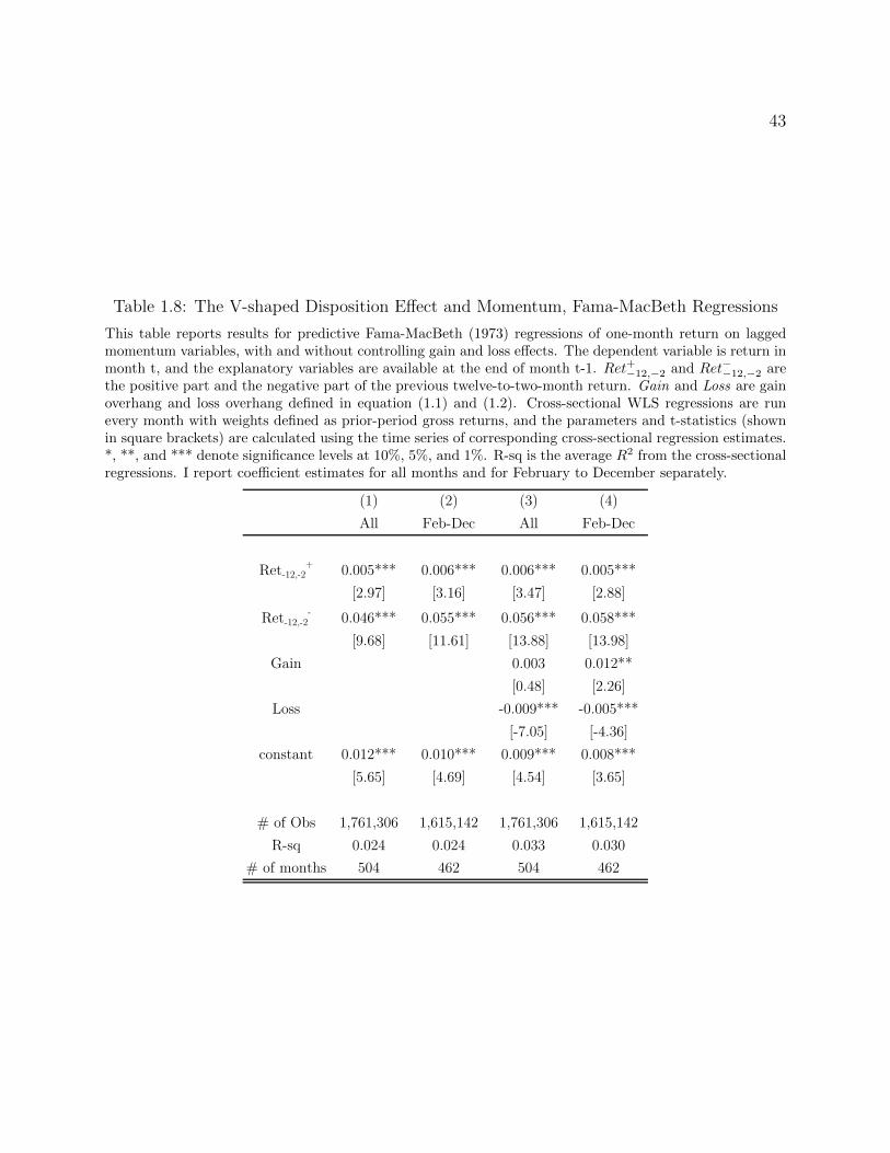
43

Table 1.8: The V-shaped Disposition Effect and Momentum, Fama-MacBeth Regressions

This table reports results for predictive Fama-MacBeth (1973) regressions of one-month return on laggedmomentum variables, with and without controlling gain and loss effects. The dependent variable is return inmonth t, and the explanatory variables are available at the end of month t-1. Ret+−12,−2 and Ret−−12,−2 arethe positive part and the negative part of the previous twelve-to-two-month return. Gain and Loss are gainoverhang and loss overhang defined in equation (1.1) and (1.2). Cross-sectional WLS regressions are runevery month with weights defined as prior-period gross returns, and the parameters and t-statistics (shownin square brackets) are calculated using the time series of corresponding cross-sectional regression estimates.*, **, and *** denote significance levels at 10%, 5%, and 1%. R-sq is the average R2 from the cross-sectionalregressions. I report coefficient estimates for all months and for February to December separately.

(1) (2) (3) (4)All Feb-Dec All Feb-Dec

Ret-12,-2+ 0.005*** 0.006*** 0.006*** 0.005***

[2.97] [3.16] [3.47] [2.88]Ret-12,-2

- 0.046*** 0.055*** 0.056*** 0.058***[9.68] [11.61] [13.88] [13.98]

Gain 0.003 0.012**[0.48] [2.26]

Loss -0.009*** -0.005***[-7.05] [-4.36]

constant 0.012*** 0.010*** 0.009*** 0.008***[5.65] [4.69] [4.54] [3.65]

# of Obs 1,761,306 1,615,142 1,761,306 1,615,142R-sq 0.024 0.024 0.033 0.030

# of months 504 462 504 462

Chapter 2

V-Shaped Disposition: Mutual Fund

Trading Behavior and Price Effects

Li An, Bronson Argyle

45

2.1 Introduction

In the field of asset pricing, researchers have documented many return anomalies, each with

various potential explanations. However, pinning down the specific source of return patterns

is difficult. As John Cochrane put it in his 2010 AFA presidential address, “A crucial

question is, as always, what data will this class of theories use to measure discount rates?

... Ideally, one should tie price or discount-rate variation to central items in the models,

such as the balance sheets of leveraged intermediaries, data on who is actually active in

segmented markets, and so forth.” Behavioral theories, in particular, have applied findings

from the field of psychology to suggest that behavioral biases can cause market prices to

systematically deviate from the “rational” benchmark; yet it remains a demanding task to

empirically link investors’ behaviors to equilibrium price dynamics.

In this paper, we study how mutual fund managers’ trading behaviors affect stock prices.

We present two main findings: first, we document a behavioral pattern characterized by

mutual fund managers being more likely to sell stocks with relatively large gains and losses,

rather than those with small gains and losses; second, we construct stock-level variables

to capture the price pressure from such selling behavior, and we show that these variables

strongly predict stock returns in the cross section. By investigating the holdings data of

mutual funds, we have the advantage of observing fund managers’ trading behaviors and are

able to directly test the ensuing pricing implications. In our sample, we find price pattern

dynamics that are robustly consistent with the cross-sectional variations of the documented

selling behavior.

This research bears on the most recent studies of the disposition effect. First introduced

to the finance literature by Shefrin and Statman (1985), the disposition effect refers to in-

vestors’ tendency to sell their winning securities more readily than their losers. Since then,

46

this trading behavior has been widely documented using evidence from both individual and

institutional investors1, across different asset markets2, and around the world3. Previous re-

search mostly focuses on the difference in selling propensity when investors experience a gain

versus a loss, rather than the full functional form of how investors trade in response to past

profits. In a recent study, Ben-David and Hirshleifer (2012) take a close look at individual

trading account data (as in Odean (1998)) and document a refinement of the disposition

effect: counterintuitively, individual investors do not increase their selling probability mono-

tonically from the extreme losers to the extreme winners; instead, they have a V-shaped

selling schedule in response to past profit. Moreover, the gain side of the V is steeper than

the loss side of the V, thus the average propensity to sell following a gain is higher than the

average propensity to sell following a loss.

We examine the selling schedule of mutual fund managers in response to unrealized

profits. While studying individual traders is interesting in order to understand investors’

trading behavior, mutual fund managers tend to represent more capital, resemble more of

a representative investor, and are more important in deciding the market price. We find

that mutual fund managers, like individual traders, exhibit a V-shaped selling schedule, i.e.

the probability that managers sell a particular security increases with the magnitude of the

unrealized gain or loss of that security.

We argue that such trading behavior can generate price pressure and subsequent return

predictability in the cross section. As mutual fund managers are more likely to sell stocks

1See Odean (1998) and Grinblatt and Keloharju (2001) as examples for individual investors. See Lockeand Mann(2000), Shapira and Venezia (2001), and Coval and Shumway (2001) for institutional investors.

2See, for example, Genesove and Mayor (2001) in housing markets, Heath, Huddart, and Lang (1999) forstock options, and Camerer and Weber (1998) in experimental markets.

3See Grinblatt and Keloharju (2001), Shapira and Venezia (2001), Feng and Seasholes (2005), amongothers. For a thorough survey of the disposition effect, please see the review article by Barber and Odean(2013).

47

with large gains and losses (compared with stocks with modestly unrealized gains and losses),

it increases the supply of such stocks and in turn presses the equilibrium price down from

its fundamental value. As future price reverts back to the fundamental value, stocks with

large gains and losses will outperform others in the subsequent periods.

To test this hypothesis, we construct price pressure variables directly from mutual fund

holdings data. We follow the methodology developed by Frazzini (2006) to measure the

aggregate cost base for a particular stock using the time series of net purchases across the

mutual fund universe. Taking into account investors’ V-shaped selling schedule, we separate

unrealized gains from unrealized losses. Empirical results confirm our hypothesis: stocks

with large gain overhang and large loss overhang indeed outperform in the next month,

and the price effect is both economically and statistically significant: a 1 percentage point

increase in the aggregate unrealized gains (losses) for a stock predicts a 1.5 (0.8) basis point

increase in the next month return. A trading strategy based on this effect can generate a

Sharpe ratio of 1.4. These result are consistent with price effects documented by An (2014),

where investors’ aggregate cost base is approximated based on trading volume.

To better establish the link between investors’ trading behavior and the price pattern,

we conduct a series of tests to explore the cross-sectional variation in mutual funds’ trading

behaviors, and we test if the return predictability mostly comes from the positions of those

who exhibit the strongest V-shaped selling schedule. For example, we find that more spec-

ulative mutual fund managers, characterized by having a shorter average holding period of

stocks and having a higher turnover ratio, tend to have a steeper V-shaped selling schedule;

we then decompose our overhang variables into unrealized gains and losses from speculative

funds and those from “nonspeculative” funds. We find the former overhang variables are

stronger in predicting future returns. Our dataset and our chosen way to measure selling

pressure allow us to pin down the source of return predictability. These tests closely tie the

48

variation in price pattern to the variation in investor behavior, and it is a unique contribution

of our paper.

We contribute to the literature on the disposition effect in two ways. First, on top

of the empirical regularity that investors sell more winners than losers, we document the

full functional form of how investors trade in response to past profit. The evidence of a

V-shaped selling schedule among mutual fund managers corroborates the findings by Ben-

David and Hirshleifer (2012) for individual traders. The V shape in investors’ selling schedule

is important for two reasons. First, it refutes the common presumption that investors’

selling propensity monotonically increases with their past profit, upon which much empirical

work has been based. Moreover, it calls into question commonly offered explanations for

the disposition effect. Prevalent theories, either prospect theory (Kahneman and Tversky

(1979)) that states investors are loss-averse, or the realization utility developed by Barberis

and Xiong (2009, 2012), all rely on the point that investors derive a higher utility by realizing

gains rather than losses; however, while these preference-based interpretations can generate

a monotonic selling schedule, they can hardly reconcile the V shape in investors selling

schedule.

Second, this paper expands our understanding of the pricing implications of the dispo-

sition effect. The early literature is exclusively based on the premise that investors have a

monotonic selling schedule. For instance, Grinblatt and Han (2005) develop an equilibrium

model where the disposition effect influences investors’ demand for a stock and in turn causes

the equilibrium price to deviate from the fundamental value in a predictable way. They show

that capital gains overhang, a empirical measure that linearly aggregates all investors’ un-

realized gains and losses, predicts future returns. Frazzini (2006) constructs a capital gains

overhang measure using mutual fund holdings data and shows that the disposition effect can

cause price underreaction to news. Pricing implications of the V-shaped selling schedule has

49

only been taken into account very recently - motivated by Ben-David and Hirshleifer (2012),

An (2014) separates the capital gains overhang of Grinblatt and Han (2005) into gain over-

hang and loss overhang, and finds that stocks with both large unrealized gains and losses

outperform in the next month. Her measures for unrealized gains and losses, as in Gainblatt

and Han (2005), are aggregate approximations based on trading volume. Our measure em-

ploys the mutual fund holdings data and is thus able to track accurate unrealized positions

for this important group of investors. This methodology is meant to eliminate the ambiguity

in using aggregate approximate measures; moreover, it allows us to further explore the link

between mutual fund managers’ trading behavior and price impact.

Our paper also extends the literature on the price impacts of mutual fund managers’

uninformed trades. Among others, Coval and Stafford (2007) show that mutual funds who

experience large outflows are forced to decrease existing positions and this creates price

pressure on stocks that are commonly held by distressed funds. Argyle (2013) finds that

idiosyncratic shocks to a firm in mutual fund’s portfolio can induce portfolio flows and cause

price pressure on other firms in common portfolios. Overall, most of the documented price

effects are due to the liquidity channel4 and imply the agency problems and institutional

constraints modeled by Shleifer and Vishny (1997). On the contrary, the price impact found

in our paper is orthogonal to flow controls; in this paper, the behavioral tendencies of mutual

fund managers is the source of the price deviation from fundamentals.

The rest of the paper is organized as follows. Section 2 provides on overview of the

datasets used. Section 3 constructs the necessary variables and outlines the specification

strategy. Section 4 discusses the results. Section 5 examines heterogeneity across funds and

the resulting cross-sectional variation in selling behavior and pricing implications. Section 6

4See Blocher (2011), Hau and Lai (2011), Hau and Lai (2012), Lou (2012), and Anton and Polk (2013),among others.

50

explores various robustness checks of the main finding. Section 7 concludes.

2.2 Data description

Data are collected from three datasets. Mutual funds holding data are taken from the

Thomson Reuters Mutual Fund and Institutional Holdings databases from the S12 and

S34 Master Files. The data span the time series from January 1980 to December 2012,

inclusively. These data are crosschecked at the fund-date level against the CRSP Mutual

Fund Summary database as discussed below. The CRSP Mutual Fund Summary database

is also used to construct some of the fund-date level control variables. Security price and

accounting information are taken from the CRSP Security File. We include all common

shares of domestic securities corresponding to a share code of 10 or 11 which excludes ADRs,

ATCs, REIT, and closed-end funds. Similar to previous literature, we employ the following

filters:

1. We exclude all fund-date combination in which the Total Net Assets reported by Thom-

son Reuters differs from the CRSP database by more than 100%.

2. We exclude all fund-date-holding combinations in which the number of shares of a firm

i reported to be held by a given fund exceeds the number of shares outstanding of firm

i on a given date.

3. We exclude all fund-date-holding combinations in which the market value of a reported

holding of a firm i exceeds the Total Net Assets of the reporting fund on a given date.

4. We exclude all fund-date-holding combinations in which the price of one share of the

security is below $2.

51

Applying these filters results in roughly 20M valid fund-quarter-holding combinations for

which price data exists from CRSP. We assume that holdings are constant during the quarter

and that all trading takes place at the end of the reporting quarter. Numerous work has

discussed and demonstrated the reality of intraquarterly trading5, but given that the ratio

of the size of trading to Total Net Assets is relatively small, we abstract away from these

realities to focus on the capital overhang effects. At best, daily trading simply adds noise

to our estimation, and at worst it biases against our results. Further, as discussed in the

CRSP/Compustat manual, fund numbers (variable “fundno”) are often reused for unrelated

funds; we assume that a gap of more than 2 years between reporting dates implies the

cessation of the previous fund and the outset of a new fund.


2.3 Specification

2.3.1 Trading Behavior

To identify the v-shaped disposition effect directly in the trading behavior of fund managers,

we construct two sets of two measures of the holding period overhang. Our primary measure

of the holding period overhang for a given security in the portfolio of fund f in period t, is

given by

hp overhangft =t∑

n=0

Vf,t,t−n∑tn=0 Vf,t,t−n

[pt − pt−n

pt

](2.1)

where Vf,t,t−n is the number of shares purchased of the security at time period t−n that are

still held in the fund at time period t, and pt is the price of the security at time period t.

5See Busse (1999), Bollen & Busse (2001), Green & Hodges (2002), Puckett and Yan (2011), Bobson,Cavenaile, & Sougn (2012), and Argyle (2013).

52

Intuitively, the overhang variable is capturing the average deviation of the current price from

the purchase price (pt − pt−n) as a percentage of the current period’s price (pt), weighted

by the number of shares purchased in a given period that are still currently held (Vf,t,t−n).

We follow the argument laid out in Frazzini (2006) and employ a First In First Out (FIFO)

assumption to populate Vf,t,t−n - the mental accounting of fund managers. When part (or

all) of a position is sold, shares are sold in the order that they were purchased. For example,

if in time period 0, the fund manager of a given fund purchases 500 shares of a security, and

in time period 1 she adds another 1000 shares, then the fund manager now owns 1500 shares,

and the net positions for the fund are given by Vf,1,0 = 500 and Vf,1,1 = 1000. If the fund

manager decides to sell 700 shares in time period 2, then we would assume that the shares

that were purchased first are sold first, such that Vf,2,0 = 0, Vf,2,1 = 800, and Vf,2,2 = 0.

To be consistent with the construction of the capital overhang variables (discussed below),

the denominator of the unweighted component of hp overhangt is the current price (as

opposed to the purchase price). In this way, hp overhangt is simply the capital overhang

at the fund-holding level. We will also examine an alternative measure normalized by the

purchase price.

In order to examine a V-shaped disposition effect, we further separate the holding period

overhang into unrealized gains and losses for a given security in the portfolio of fund f at

time t:

hp gainft =t∑

n=0


[(pt − pt−n) Ipt−n≤pt

pt

](2.2)

and

hp lossft =t∑

n=0


[(pt − pt−n) Ipt−n>pt

pt

], (2.3)

where the indicator variables Ipt−n≤pt and Ipt−n>pt indicate that the current price is greater

than or equal to the purchase price and that the current price is less than the purchase

53

price, respectively. This construction implies that hp overhang = hp gain + hp loss, for

every fund-security-period. We also construct the variable hp time to capture the weighted

average amount of time that the shares have been held. For a given security, this is defined

as:

hp timeft =t∑

n=0


[t− n] . (2.4)

Our primary selling specification, similar to Ben-David and Hirschleifer (2012), is thus a

logit regression:

I(selling)fit = α + β+hp gainfit + β−hp lossfit +

ζ+hp gainfit ∗√hp timefit + ζ−hp lossfit ∗

√hp timefit (2.5)

+ζ√hp timefit + Controlsfitγ + εfit

where Controlsfit is a vector of fund-level and security-level control variables and γ is a

vector of corresponding coefficients. We exclude all months that are not reporting months

for the fund; we do this to address potential concerns that our observed effect is mechanically

influenced by our assumption that holdings are constant between reporting months. We

also exclude outlier funds whose Total Net Assets is in either .5% tail. As an exploration of

robustness, we use fund-level flow at various horizons (when data permit) and daily security-

level volatility calculated over the previous year as controls.

2.3.2 Price Effect

In our primary analysis of the pricing implications of a V-shaped disposition effect, the

capital gains overhang for a given security at time t is calculated at a monthly horizon and

54

is defined analogously:

overhangt =pt − rptpt

, (2.6)

where pt is the single share price of the given security at time t, and rpt is the corresponding

reference price. The reference price (rpt) is defined as:

rpt =

∑tn=0 Vt,t−npt−n∑tn=0 Vt,t−n

, (2.7)

where Vt,t−n is the aggregate sum of the shares purchased at time t−n that are still held

at time t across all funds:

Vt,t−n =F∑f=1

Vf,t,t−n, (2.8)

and F is the total number of funds. We construct the capital gains overhang due to un-

realized gains and unrealized losses similar to the fund-level variables such that overhang =

gain overhang + loss overhang, for every security-period. The overhang due to gains and

losses are defined as:

gain overhangt =t∑

n=0

Vt,t−n∑tn=0 Vt,t−n

[(pt − pt−n) Ipt−n≤pt

pt

](2.9)

and

loss overhangt =t∑

n=0

Vt,t−n∑tn=0 Vt,t−n

[(pt − pt−n) Ipt−n>pt

pt

](2.10)

In order to examine the pricing implications of a V-shaped disposition effect, we consider

two empirical models. The first model estimates how gain overhang and loss overhang predict

55

future returns separately :

Reti,t = α + β1gain overhangi,t−1 + β2loss overhangi,t−1 + γ1Ctrl1i,t−1 + γ2Ctrl2i,t−1 + εi,t,

(2.11)

We expect β1to be positive, β2 to be negative, and the relation between these two price effects

(β1β2

) to match the relative selling sensitivity we find in the selling behavior regressions.

To put our finding into context of the literature, we further pit the linear CGOi,t (Capital

Gains Overhang as in Frazzini (2006)) against our V-shaped construction V-shaped Selling

Pressure (VSP), defined as (gain overhangi,t + φ|loss overhangi,t|), where the parameter φ

is the relative relationship between selling pressure from unrealized gains and from unrealized

losses. We consider the following model:

Reti,t = α + β1CGOi,t−1 + β2V SPi,t−1 + γ1Ctrl1i,t−1 + γ2Ctrl2i,t−1 + εi,t, (2.12)

Our results from the selling behavior regressions (expressed in equation 2.5) suggest that

mutual fund managers are twice as likely to sell a gain as to sell a loss with the same

magnitude, thus we expect a gain overhang to result in twice the selling pressure as a

similarly sized loss overhang. We take φ equal to 0.5.

We are concerned that the overhang variables may correlate with other return predictors,

and we include two sets of control variables in our estimates of the price effect. The first set

of controls (Ctrl1i,t−1) is designed to control for the momentum effect. As we would expect,

stocks with large unrealized gains (losses) tend to be those who performed well (poorly) in

the past, and the past one year return is a well-documented predictor of future return (see

Jegadeesh (1990) and Jegadeesh and Titman (1993)). Thus, we include the past 12-to-2

month return, but we separate the raw return by sign: Ret+i,t−12,t−2 = Max{0, Reti,t−12,t−2},

56

and Ret−i,t−12,t−2 = Min{0, Reti,t−12,t−2}. We do this to address the asymmetry of momen-

tum’s predictive power - Hong, Lim, and Stein (2000) find that the loser leg of momentum

is markedly stronger than the winner leg in predicting future return which implies that the

raw return may not be a good functional form for capturing the proper return-momentum

relationship. This is particularly relevant for our purpose, because if we artificially equate

the coefficient for momentum winners and momentum losers, the rest of the predictive power

may be picked up by our gain/loss overhang.

Besides momentum, we also control for other common return predictors in Ctrl2i,t−1

which includes the following variables. The past one month return (Reti,t−1) and the past 3-

to-1 year return (Reti,t−36,t−13) address the potential contamination from short-term reversal

and long-term reversal, respectively. ivol is the idiosyncratic volatility with respect to a

Fama-French three factor model calculated using daily stock return data in the past one

year. logBM is the logarithm of the book-to-market ratio; the calculation follows Daniel

and Titman (2006) in which this variable remains the same from July of year t through

June of year t + 1, and there is at least a 6 months lag between the fiscal year end and the

measured return to allow enough time for this information to become public. logMktcap is

the logarithm of a firm’s market capitalization. turnover is the average daily turnover ratio

( trading volumeshares outstanding

) in the past one year; this is meant to capture any volume effects that may

relate to future returns6.

We conduct predictive Fama-MacBeth regressions. To avoid the liquidity bias in esti-

mations, we follow the suggestion by Asparouhova, Bessembinder, and Kalcheva (2010) and

run weighted least square (WLS) regressions with the weight equal to past one-month gross

return. OLS results (omitted to save space) are qualitatively the same, suggesting that liq-

uidity bias is not a severe issue in our exercises. We follow An (2014) and run tests using all

6See Lee and Swaminathan (2000) and Gervais, Kaniel, and Mingelgrin (2001)

57

months as well as excluding January, to demonstrate that our results are not driven by the

January effect7.

Finally, it is important to discuss the timing of information availability. Holdings data

that are reported by Thomson Reuters stipulate both the effective date of holdings data

(variable “rdate”) as well as the date that these holdings were filed with the SEC (variable

“fdate”). It is not uncommon, especially in the early sample, for the difference between

when the information is relevant (rdate) and when it is reported (fdate) to be severe (up

to 24 months in extreme cases). This is seemingly less common in the latter portion of

the data. Though the selling behavior can and should be identified using the data as of

the corresponding rdate, the correct course of action is less clear when examining the price

effect regressions (equations 2.11 and 2.12). While using the holdings data as of the rdate is

justifiable to identify a pure price effect, these results would not speak to a viable trading

strategy. To this end, for the selling behavior regressions, we use the data as of the corre-

sponding rdate, but for the price effect regressions we estimate holdings based on the most

recent filing date (with at least a 1 month lag). This is identical to the argument formulated

in Frazzini (2006) and ensures that overhang data are publicly available.

2.3.3 Alternative Measures

We propose an alternative measure of the overhang that is consistent with the usual definition

of returns - we normalize based of the purchase price instead of the current price. This

7For tax purposes, investors in December tend to sell off losing stocks to offset capital gains. The priceof such stocks tends to decline in December and then reverses in January. See, for example, Roll (1983),Lakonishok and Smidt (1988), and Grinblatt and Keloharju (2004).

58

alternative holding period overhang is thus calculated as:

hp overhang altft =

∑tn=0 Vf,t,t−n (pt − pt−n)∑t

n=0 Vf,t,t−npt−n, (2.13)

and the alternative fund-security overhang variables are constructed accordingly:

hp gain altft =

∑tn=0 Vf,t,t−n (pt − pt−n) Ipt−n≤pt∑t

n=0 Vf,t,t−npt−n(2.14)

and

hp loss altft =

∑tn=0 Vf,t,t−n (pt − pt−n) Ipt−n>pt∑t

n=0 Vf,t,t−npt−n. (2.15)

Similarly, this implies that the alternative pricing effect overhang is defined as

overhang altt =pt − rptrpt

, (2.16)

and the alternative gain and loss overhang variables for a given security (where the Vf,t,t−n

are aggregated across funds) are:

gain overhang altt =

∑tn=0 Vt,t−n (pt − pt−n) Ipt−n≤pt∑t

n=0 Vt,t−npt−n(2.17)

and

loss overhang altt =

∑tn=0 Vt,t−n (pt − pt−n) Ipt−n>pt∑t

n=0 Vt,t−npt−n. (2.18)

We argue that the measures normalized by current price (pt) are preferred, because the

overhang variables are then weighted averages of the deviations from the purchase prices.

The alternative measure offers no such intuitive interpretation, though it is consistent with

the usual definition of holding period returns.

59

2.4 Results

2.4.1 Trading Behavior

Results from the selling behavior regressions are shown in Table 2.2. All errors are clustered

at the fund level except regression 6, where the errors are two-way clustered at the fund-time

level. The results from regression (1) shows a strong overhang effect. We see that both the

hp gainfit (4.10) and hp lossfit (-1.64) coefficients are strongly significant with t-stats of

43.4 and -38.1, respectively. The magnitude of these coefficients implies that a 1% increase

in the holding period gain implies a 4.1% higher probability that some or all of the security

will be sold this period. A 1% more extreme holding period loss implies a 1.6% higher

probability of being sold. These results confirm the V-shaped disposition effect, and the

relatively magnitude (1.644.10

= .4) further suggests an asymmetric V-shaped effect. Regressions

(2) and (3) repeat this regression, but separate the sample based on “short” holding period(√hp time ≤ 3.5

)and “long” holding period

(√hp time > 3.5

). Both subsamples manifest

a strongly V-shaped disposition effect - the ratio of loss to gain coefficients(∣∣∣ hp losshp gain

∣∣∣)is equal

to .32 for short holding periods and .51 for long holding periods. However, the magnitude

of the coefficients and the corresponding t-stats are bigger for shorter holding periods.

Regressions (4) and (5) split the data into a “past” subsample spanning 1980 to 2001 and

a “recent” subsample spanning 2002-2012. We see that coefficient estimates are qualitatively

identical to the original regression with t-stats above 30, though the magnitude of the results

in the recent sample is slightly smaller. Regression (6) uses the logit2 code written by Jingling

Guan and Mitchell Petersen (2008) to perform logit regressions using two-way clustering at

the fund-quarter level. T-stats are reduced (as expected), but remain highly statistically

significant. Finally, regression (7) is a further robustness check including an outflow dummy

equal to 1 if the monthly flow of the fund is less than zero and an interaction between

60

outflow and the holding period overhang. The usage of the flow data reduces the sample to

only those funds in the CRSP universe for which flow data can be calculated (reducing the

number of observations from roughly 20.4 million to 7.4 million). The resulting coefficient

estimates have slightly smaller magnitudes (3.64 for the holding period gains and -1.37 for

the holding period losses), but are very close to the original estimates. We also explore

various windows for the measurement of the fund flows, at 3 month and 12 months horizons,

without notable change in the coefficient estimates (results omitted). We conclude that the

observed V-shaped disposition effect is orthogonal to fund flow effects8


2.4.2 Pricing Effect

In this section, we discuss the empirical pricing implications of mutual fund managers’ V-

shaped selling schedules. We first estimate how gain overhang and loss overhang predict

future return separately. Then, using the selling behavior regressions as our guide, we

combine the gain and loss overhang estimates in order to capture the V-shaped disposition

effect in a single variable. We pit this variable against the capital gains overhang variable

found in previous literature.

Table 2.3 presents results from estimating equation 2.11 using Fama-MacBeth regressions.

In these regressions, we expect gain overhang and loss overhang, the variables of our main

interest, to have a positive coefficient and a negative coefficient, respectively. Note that

by construction, all values of the loss overhang variable are negative, so an increase in loss

overhang means a decrease in the magnitude of loss. Regressions (7) and (8) are the full

model regressions with all proper controls. Regressions (1) through (6) omit various sets

8See Lou (2012) for an example of the effects of fund flows on mutual fund trading behavior.

61

of control variables to gauge the relative importance of different price effects. In columns

(1) and (2), we regress future one-month return onto gain overhang and loss overhang only,

and we see that the coefficients on loss overhang (0.002 in all months, and 0.004 in Feb

to Dec) have opposite signs than expected. This is due to the fact that stocks with large

unrealized losses tend to be momentum losers, and failing to properly control for momentum

masks the true marginal effect of the overhang variables. Indeed, adding the two legs of

momentum, Ret+−12,−2 and Ret−−12,−2, we see in regressions (3) and (4) that the gain and loss

overhang variables have the expected sign. Notably, the coefficient for Ret−−12,−2 is roughly

an order of magnitude larger than the coefficient for Ret+−12,−2. This suggests that the loser

leg of momentum is indeed markedly stronger than the winner leg and that it is important

to separate the momentum return by sign to capture the true price effect. In regressions

(5) and (6), we omit momentum controls and add other common return predictors (Ctrl2).

Finally, regressions (7) and (8) add all relevant controls and present our best estimations.

In these two regressions, gain overhang positively predict future return and loss overhang

negatively predict future return, both as expected; focusing on the all-month estimation, the

coefficients suggest that a 1 percentage point increase in gain (loss) overhang would cause a

1.4 (0.9) basis point increase (decrease) in the next month return. The t-statistics (6.02 and

-8.65) are very large - given 391 months are used in the estimation, these numbers imply that

a trading portfolio based on gain (loss) overhang with zero loading on other control variables

would have a Sharpe ratio of(

6.02√

12391

)= 1.05 and

(8.6√

12391

)= 1.51, respectively.

Grinblatt and Han (2005) discuss the important relation between momentum effect and

capital gains overhang; in fact, they find that capital gains overhang subsumes momentum

in their sample and suggest that the disposition effect may be the source of momentum. On

the contrary, An (2014) argues that, if investors tend to sell big loser as well as big winners,

the loss part of capital gains overhang will predict future return in the opposite direction as

62

momentum would. This claim is also supported by empirical evidence by Novy-Marx (2012)

and Birru (2012). Our results here support the second view that disposition effect can not

be the source of the momentum effect, as loss overhang and the loser leg in momentum have

opposite return predictions.

We also draw attention to the relationship between idiosyncratic volatility and the over-

hang effects. It has been documented that high idiosyncratic volatility stocks are associated

with low future returns9, and perhaps unsurprisingly, stocks with large gain and loss over-

hang tend to be those with high idiosyncratic volatility. This result actually biases against

our results since our model predicts the opposite direction than what ivol would: stocks with

large gain and loss overhang will outperform in the next month as prices return to funda-

mentals. Indeed, controlling for idiosyncratic volatility strengthens the predictive power of

our overhang variables - note the change in overhang coefficient estimates from columns (1)

& (2) to columns (5) & (6) and the change from columns (3) & (4) to columns (7) & (8).


[To be added: subsample results (1980-2001, 2002-2012) of pricing effects]

To compare and contract with previous literature, we first construct a single V-shaped

selling pressure variable, V-shaped Selling Pressure (VSP), equal to (gain overhang+φ|loss overhang|)

with φ = .5. We conduct a horse race between VSP and the linear Capital Gains Overhang

(CGO) variable as in Frazzini (2006). Table2.4 presents the results. We see that with control

variables included, CGO loses all of its predictive power, while VSP remains highly signifi-

cant. The coefficient of 0.016 in the all-month estimation suggests that a 1 percentage point

increase in VSP would lead to 1.6 basis point increase in future one-month return; given

that the average 10th and 90th percentile of monthly VSP sample is 0.04 and 0.36, a port-

9see Ang, Hodrick, Xing, and Zhang (2006, 2009), among others

63

folio that longs the top VSP quintile and shorts the bottom VSP quintile would generate a

monthly return spread of approximately (36 − 4) × 1.6 = 51.2 basis points. The t-statistic

= 8.44, which implies that the Sharpe ratio is around 8.44/√

391×√

12 = 1.47.


2.4.3 Alternative Measures

We explore the alternative measure of holding period overhang which is normalized by pur-

chase price instead of current price. This definition is more consistent with the usual for-

mulation of holding period return. Previous literature has focused solely on the original

measure of overhang (normalized by current price) and has failed to explore this interesting

alternative. Selling behavior results are shown in Table 2.5. Many of the observations drawn

using the original measures are maintained. We see highly significant overhang coefficients

that persist throughout a number of subsample and error-clustering specifications. Also,

results are much more prevalent for shorter holding periods (regression (2)) than for longer

holding periods (regression (3)) which is consistent with the findings presented earlier. The

most interesting observation from these results is that the overhang coefficients are still very

statistically and economically significant, but the relative magnitude between holding period

gain and loss is opposite the original measure. From regression (1), we see that the ratio of

coefficients∣∣∣ hp losshp gain

∣∣∣ = 1.71. This relationship is consistent across all of the selling behavior

regressions for the alternative measures.


We examine the pricing effects of the alternative measure in Table 2.6. Interestingly, we

see when using the alternative measures, the relative impact of the gain overhang and the

64

loss overhang have reversed from the previous results - consistent with the selling behavior

regressions using the alternative measures. In the fully controlled regressions (7) and (8),

the significant gain and loss coefficients (t-stats are greater than 7) are .0115 and -.0225,

respectively, in the all-months case.


These results further instantiate the robustness of the V-shaped disposition effect. Though

the relative slope of the gain and loss overhang is dependent on the choice in normalizing

price, both measures result in statistically and economically significant coefficient estimates

whose predictions for fund managers’ selling behavior are consistent with the estimated

effects on equilibrium price.

2.5 Exploring the link: how heterogeneity in mutual

funds’ behavior affects price patterns

As a further exploration of the source of the V-shaped disposition effect, we repeat the selling

behavior regressions on subsamples of the fund universe, splitting the data based on fund

characteristics designed to capture inefficiencies and speculation in the fund manager. These

characteristic variables are the expense ratio, the management fee, the turnover, and the

average holding period within a portfolio. The expense ratio is the ratio of operating expenses

to total investment. Management fee is the ratio of fees, as reported in the Statement of

Operations, to the Average Net Assets($). The turnover is the ratio of aggregated purchases

($) divided by the average 12-month Total Net Assets. Fund characteristics data are only

available for the subset of funds that are in the CRSP Mutual Fund database, and the

universe is reduced to roughly 7.4 million fund-holding-period observations.

65

A given portfolio that is included in the CRSP database will have almost always (at most)

a single corresponding fund in the Thomson Reuters data. However, the same portfolio may

correspond to several separate share classes (varying fee structures, eligibility requirements,

etc.) in the CRSP database. Treating these share classes as separate portfolios would bias

the results towards funds with more share classes. To address this bias, we instead construct

weighted averages of the characteristic variables based on the Total Net Assets of the various

share classes. For example, consider a single portfolio with two share classes: Fund A with

Total Net Assets of $400M and Fund B with Total Net Assets of $200M. Both of these funds

represent exposure to the same portfolio (and trading behavior), but they may have very

different characteristics. For instance, assume that the expense ratio of Fund A is 2% and

the expense ratio of Fund B is 5%. We thus calculate the weighted average expense ratio:

400600.02+ 200

600.05 = .03 for the portfolio. This procedure allows us to parsimonously determine

the overall average expense ratio (in the case of our example) of the fund.

Though this procedure is not without alternatives, our primary goal is simply to cate-

gorize the fund, and this procedure allows us to computationally parse the characteristics

of varied share classes in an intuitive manner. We thus obtain weighted averages of the

fund expense ratio, management fee, and turnover. Summary statistics for the weighted

versions of these variables are shown in Table 2.1 labeled as wt exp ratio, wt mgmt ratio,

wt turn ratio, respectively. We form the average holding period directly from the holdings

data using hp time.


Selling behavior results splitting funds based on the two fee structure variables (expense

ratio and management fee) are shown in Table 2.7. In both instances, we see that funds

with higher expense ratios and management fees manifest a much more significant V-shaped

66

disposition effect - the coefficient for holding period gain (hp gain) for funds in the top third

by expense ratio is a highly significant 4.27, whereas the corresponding coefficient for funds

in the bottom third by expense ratio is 2.34. The difference is statistically significant, and we

see a similar difference in the coefficients for holding period loss (hp loss). Funds sorted by

management fees, a subset of the operational costs included in the expense ratio, produces

qualitatively consistent results. To the extent that higher fees proxy for management effi-

ciency, these results suggest that the V-shaped disposition effect may be the manifestation

of inefficient management.


Selling behavior results splitting funds based on the two speculation variables (turnover

and average holding period) are shown in Table 2.8. Though these two variables are related,

they capture different aspects, and high turnover does not necessarily imply low average

holding period. We find that the V-shaped disposition effect is much more severe amongst

funds with higher trading turnover and short average holding period: the gain and loss

coefficients for high turnover funds (5.1 and -2.1, respectively) are roughly twice the size of the

gain and loss coefficients for funds with low relative turnover (2.43 and -0.93, respectively).

Similarly, funds with the shortest average holding period have coefficients almost twice the

magnitude of funds with the longest average holding period. These results suggest that

relatively active managers are more prone to evince a V-shaped disposition effect.

67

2.6 Robustness checks

2.6.1 Extreme Rank Dependency

There is some evidence that if a security is the absolute best performer in a portfolio or the

absolute worst performer in a portfolio, then it is treated and traded materially differently by

the manager. See Hartzmark (2013). To address this concern, we rerun the primary selling

regression and include a dummy variable signifying that the security is the best performing

in the portfolio in a given period (best dummyfit) and also a separate dummy variable if the

security is the worst performing in the portfolio in a given fund (best dummyfit), defined in

the following manner:

best dummyfit =

1 if security ihas the highest hp overhang

in the portfolio of fund f in period t

0 otherwise

(2.19)

and

worst dummyfit =

1 if security ihas the lowest hp overhang

in the portfolio of fund f in period t

0 otherwise

. (2.20)

We also control for the universe-of-funds-wide versions of the Hartzmark dummies in the

pricing effect regressions, constructed according to:

best dummyi,t =

1 if security ihas the highest hp overhang

in the portfolio of at least one fund in period t

0 otherwise

(2.21)

68

and

worst dummyi,t =

1 if security ihas the lowest hp overhang

in the portfolio of at least one fund in period t

0 otherwise

. (2.22)


Selling behavior regressions using both the original and alternative measures that include

these dummies are shown in Table 2.9. Regression 1 repeats the main regression without

subsample splits. Both the coefficient estimates and the resulting ratio of gain and loss coeffi-

cients are practically unchanged from the regressions omitting these extreme rank dummies.

Regression 2 substitutes the alternatives measures and finds similar results. Those these

dummies do not effect our overhang findings, the corresponding coefficient are persistently

significant even when controlling for fund flow variables at 1 month, 3 month, and 12 month

horizons (results omitted). The standardized coefficents for the best dummy is equal to

.0938 .497.494

= .0944 whereas the standardized coefficient of the hp gain variable is equal to

3.9974 .128.494

= 1.04. Also, the R2 improvement from adding these rank dummies is minimal

(.0129 versus .0112).

We also find that including the similar security-level dummies in the pricing equations

has virtually no qualitative effect on the overhang coefficient estimates. These results are

shown in Table 2.10.


69

2.6.2 Simple Measures

We examine a two simpler measures of overhang in which fund managers consider the un-

weighted overhang based on purchase price of only the “oldest” shares that have not yet been

sold. We examine both the original measure (normalized by current price pt) and also the

alternative measure (normalized by the purchase price). Given the FIFO assumption about

the construction of Vf,t,t−n, managers only consider the purchase price (pt−n) associated with

the nonzero value of Vf,t,t−n with the greatest value of n. That is:

hp overhang simpleft =pt − pt−n∗

pt, (2.23)

and

hp overhang alt simpleft =pt − pt−n∗

pt−n∗, (2.24)

where n∗ = max(n) such that Vf,t,t−n > 0. We construct the holding period gain and loss

variables similar to the original construction:

hp gain simpleft =[pt − pt−n∗ ] Ipt−n≤pt

pt(2.25)

and

hp loss simpleft =[pt − pt−n∗ ] Ipt−n>pt

pt. (2.26)

70

The corresponding simple alternative measures hp gain alt simpleft and hp loss alt simpleft

are constructed similarly, though normalized by the purchase price (pt−n∗) instead of the cur-

rent price (pt) .

We similarly construct the simpler measures of the holding period :

hp time simpleft = t− n∗. (2.27)

We examine the same logit selling regression as before (equation 2.5) but use the simple

measures of holding period overhang (based on the “oldest” surviving holding of a security

according to a FIFO assumption). Results are shown in Table 2.11. We see that for both the

main and alternative measures, the coefficients of the simple versions are within an order of

magnitude of the original weighted measures. Though the t-stats are still highly significant

(above 7), they are much lower than the original measures. This suggests that fund managers

are much more inclined to process overhang that is based on the average of the purchase

prices as opposed to simply the original price. We interpret this as justification for the

original, V -weighted versions of the overhang measures. The relative magnitude, however,

of∣∣∣ hp loss althp gain alt

∣∣∣ = .55 is very similar and suggests and similar v-shaped disposition structure.

Further, if we include a flow variable directly (regression (2)), we see that though the number

of observations is nearly cut in half due to data constraints, the magnitude and statistical

significance of the overhang coefficients are qualitatively unchanged.


71

2.6.3 Placebo Test

We would predict that the disposition effect would not be observed among passive index

funds, given that these funds are not making active trading decisions. We test this hypoth-

esis by first isolating the index funds from our sample. The CRSP Mutual Fund database

categorizes index funds into three distinct groups: (B) funds are “mostly” index funds but

engage in an amount of active trading, (D) funds are “pure” index funds, and (E) funds seek

to augment or lever exposure to an underlying index. We focus our placebo test on those

(D) funds that are not open to investors. Selling occurs in these funds when the underlying

index is rebalanced - which usually occurs with a frequency of between every month and

every six months, depending on the fund. There are 71 pure index funds spanning 43,933

observations in our sample.


Results from the selling behavior regressions, using on this subset of mutual funds are

shown in Table 2.12.

2.7 Conclusions

This paper has sought to robustly establish two contributions to the current literature. First,

we have shown that mutual fund managers, like the individual retail investors of previous

research, also exhibit a V-shaped disposition effect - they are more likely to sell both their past

72

relative winners and losers. We found that the slope of the selling schedule for past winners

is roughly twice the magnitude of the slope of the selling schedule for past losers, and we

established this results using both a weighted measure of holding period overhang which took

into account the net purchases of a funds’ holdings as well as a simple measure focusing solely

on the purchase price. This discovery and these results are in contrast to the assumption of

a monotonic selling schedule proposed elsewhere in the literature. Further, we have shown

that this behavior is much more prevalent among managers whose other observable behaviors

would be considered speculative (short holding periods and high turnover relative to other

mutual fund managers). These results imply that speculation may be an underlying motive

that leads to the disposition effect. All of our results were orthogonal to a string of fund

flow variables and volatility.

The second major contribution of this research has been to demonstrate that this ob-

served behavior, aggregated across fund managers, has observable price impacts on equi-

librium prices. When properly controlling for momentum, we found that a 1 percentage

point increase in the magnitude of the gain (loss) overhang implied a 1.4 (.9) basis point

increase in future one-month returns. The relative magnitude of these effects(.9

1.44

)= .625

and(.851.54

)= .55 are completely in line with the estimates of the relative impact of holding

period gain and loss on the selling behavior of indivual mutual fund managers. With these

results in hand, we are able to directly pit a monotonic capital gains overhang measure (used

in the literature) against a V-Shaped capital gains overhang measure. Properly controlling

for momentum and short- and long-term reversal, we conducted a horse rase between the

73

two measures. The monotonic measure loses all of its predictive power (point estimate of

-.0012 with a t-stat of 1.28) against the V-shaped measure (point estimate of .0156 with a

t-stat of 8.44). The results are qualitatively unchanged if we address the January effect (the

tendency of investors to harvest losses to offset capital gains at the end of the tax year) by

excluding January observations.

We thus document both the fund manager level V-shaped disposition effect and the

accompanying price effects. We submit this result to a battery of robustness checks and

alterations, most significantly of which is an alternative overhang measure. We construct

an alternative overhang measure that normalizes price deviations by purchase price (instead

of current price). Selling behavior regression using these alternative measures of overhang

produce surprising results: though the holding period gain and loss variables continue to

be both economically and statistically significant, the relative magnitudes of their slopes is

reversed - it is now the loss overhang whose magnitude is roughly twice that of the gain

overhang. However, aggregating these measures to the security-level analogs and running

predictive pricing regressions shows that the loss overhang impact is almost twice as big as

that of the gain overhang where a 1 percentage point increase in the magnitude of the loss

(gain) overhang results in a 2.25 (1.15) basis point increase in next month returns. The ratio

of these magnitudes,(1.152.25

)= .51 is again completely consistent with the selling behavior

regressions using the alternative measure.

Finally, we expand on these findings by dividing funds on the basis of various fund

characteristics. Repeating both the selling behavior and pricing regressions, we find evidence

74

that the V-shaped disposition effect is more prevalent for fund managers with characteristics

associated with speculation (shorter holding period and higher turnover) and inefficiency

(higher expense ratios and management fees). Splitting the sample into thirds on the basis

of these characteristics, we found that the gain and loss coefficients were nearly twice as

extreme for high speculation, inefficient funds relative to low speculation, efficient funds.

75

Table 2.1: Summary Statistics.

Panel A describes the data used to examine selling behavior. hp overhang is the measure of overhangexpressed in equation 2.1. hp overhang is the alternative measure of overhang expressed in equation 2.13.I(selling) is a fund-security-period dummy equal to 1 if the part or all of the security was sold in a givenperiod. assets are the Total Net Assets of the fund expressed in thousands ($). flow1m, flow3m, andflow12m are the 1 month, 3 month, and 12 month fund flow, respectively. fret1m, fret3m, and fret12mare the 1 month, 3 month, and 12 month fund return, respectively. ivol is the average daily residual from a 3factor Fama-French model over the previous year. best dummy is a dummy equal to 1 for the highest rankedsecurity according to hp overhang in the portfolio of the fund in a given period. worst dummy is a dummyequal to 1 for the lowest ranked security according to hp overhang in the portfolio of the fund in a givenperiod. wt exp ratio, wt mgmt ratio, wt turn ratio are the weighted-average expense ratio, managementfee, and turnover ratio for the fund, respectively. outflow dummy is equal to 1 if the flow1m < 0. hp gainis the holding period gain defined in equation 2.2. hp loss is the holding period loss defined in equation 2.3.hp gain alt and hp loss alt are the alternative holding period gain and loss as defined in equations 2.14 and2.15, respectively. hp time is the net purchase-weighted holding period at the fund-security-period level.hp time alt is the corresponding alternative holding period measure. shares is the number of shares held atthe fund-security-period level.

Panel A: Summary statistics for fund-holding-level selling behavior variables.

Variable N Mean p25 p50 p75 Standard Deviation Skewness Kurtosis

hp overhang alt 20400376 -0.113 -0.251 0.02 0.2 0.538 -2.333 10.915hp overhang 20400376 -0.074 -0.185 0.016 0.157 0.399 -2.068 9.134I(selling) 20400376 0.421 0 0 1 0.494 0.321 1.103assets 16911988 91735.896 6173 20817 71955 218634.576 4.918 32.286flow1m 10729332 0.005 -0.013 -0.001 0.014 0.05 2.434 19.392flow3m 10729523 0.022 -0.036 -0.003 0.045 0.131 3.639 26.928flow12m 10732271 0.494 -0.123 0.005 0.24 4.807 21.915 564.986fret1m 10791576 0.006 -0.017 0.01 0.034 0.05 -0.436 5.653fret3m 10803061 0.021 -0.028 0.027 0.079 0.099 -0.34 4.901fret12m 10839309 0.082 -0.025 0.098 0.198 0.209 0.159 5.903

ivol 20399540 0.025 0.016 0.022 0.03 0.013 1.944 12.7best dummy 20400376 0.446 0 0 1 0.497 0.219 1.048worst dummy 20400376 0.496 0 0 1 0.5 0.016 1wt exp ratio 7954084 0.01 0.006 0.009 0.013 0.005 0.371 2.675

wt mgmt ratio 7954084 0.446 0.229 0.38 0.709 0.343 -0.135 3.484wt turn ratio 7954084 0.687 0.29 0.502 0.84 0.667 2.827 14.757

wt inst 7954084 0.537 8.644 12.674 19.756 10.951 1.947 8.315outflow dummy 20400376 0.53 0 1 1 0.499 -0.121 1.015

hp gain alt 20400376 0.15 0 0.035 0.215 0.235 2.219 8.441hp loss alt 20400376 -0.084 -0.124 0 0 0.141 -1.906 6.084hp gain 20400376 0.095 0 0.023 0.161 0.129 1.399 4.181hp loss 20400376 -0.157 -0.17 0 0 0.321 -3.212 15.393

hp time simple 20400376 4.315 2.449 3.873 5.477 2.107 1.021 3.932hp time 20400376 3.622 2.449 3.382 4.568 1.663 0.988 4.168shares 20399450 212951.2 3200 15200 70000 18742105.31 294.974 87620.163

hp gain simple 20400376 0.119 0 0.029 0.209 0.158 1.271 3.67hp loss simple 20400376 -0.223 -0.239 0 0 0.462 -3.348 16.848

hp gain alt simple 20400376 -0.118 -0.193 0 0 0.183 -1.578 4.553hp loss alt simple 20400376 0.15 0 0.035 0.215 0.235 2.219 8.441

net trading 16756850 0.102 -0.039 0 0.106 0.507 3.005 16.841I(buying) 16756850 0.307 0 0 1 0.461 0.836 1.699

76T

able

2.1:

Su

mm

ary

Sta

tist

ics

(Con

tinu

ed).

Pan

els

B&

Cd

escr

ibes

the

data

use

dto

exam

ine

pri

cin

geff

ects

.gain

overhang

and

loss

overhang

are

the

secu

rity

leve

lov

erh

ang

vari

ab

les

exp

ress

edin

equ

ati

ons

2.9

an

d2.1

0,

resp

ecti

vely

.CGO

isth

em

on

o-

ton

icd

isp

osit

ion

effec

tov

erh

ang

docu

men

ted

inF

razz

ini

(2006).

VSP

isth

eV

-sh

ap

edd

isp

osi

tion

effec

tov

erh

an

gas

isd

efin

edas

VSP

=gain

overhang

+.5|lo

ssov

erhang|.Ret

isth

eon

e-m

onth

secu

rity

retu

rn.Ret−36,−

13

isth

ela

gged

24-m

onth

retu

rn.Ret−12,−

2

isth

ela

gged

11-m

onth

cum

ula

tive

retu

rn,

andRet

+ i,t−

12,t−2

=M

ax{0,R

eti,t−

12,t−2},

an

dRet− i,t−

12,t−2

=M

in{0,R

eti,t−

12,t−2}.

logBM

isth

elo

gari

thm

ofth

eb

ook

-to-

mar

ket

rati

o.logM

ktcap

isth

elo

gari

thm

of

mark

etca

pit

ali

zati

on

.turn

over

isth

eav

erage

dail

ytu

rnov

er

rati

o( tr

adin

gvolu

me

sharesoutsta

ndin

g

) over

the

pas

tyea

r.

Pan

elB

:Sum

mar

yst

atis

tics

for

stock

-lev

elpri

cing

vari

able

s.N

mea

np25

p50

p75

Std

Skew

nes

sK

urt

osi

sgain

overhang

1164

236

0.12

10.

008

0.074

0.1

920.

135

1.38

14.7

66

loss

overhang

1164

236

-0.3

00-0

.327

-0.0

85-0

.006

0.63

1-7

.099

123.2

74

CGO

1164

236

-0.1

68-0

.299

-0.0

150.

167

0.60

4-3

.362

22.7

82

VSP

1164

236

0.17

80.

081

0.142

0.2

400.

134

1.77

89.5

02

gain

overhangalt

1164

236

0.17

00.

006

0.069

0.2

270.

294

12.

973

871.9

68

loss

overhangalt

1164

236

-0.1

60-0

.253

-0.0

86-0

.008

0.18

8-1

.361

4.2

33

CGO

alt

1164

236

0.00

6-0

.230

-0.0

150.

201

0.367

0.79

05.4

02

VSP

alt

1164

236

0.19

70.

081

0.142

0.2

400.

225

3.01

217.6

18

Ret

1164

212

0.01

2-0

.057

0.00

60.0

730.

134

0.75

27.9

09

Ret

+ −12,−

211

36148

0.25

70

0.07

90.

349

0.4

494.

417

41.3

72

Ret− −12,−

211

3614

8-0

.103

-0.1

560

00.

174

-1.8

275.6

51

Ret−12,−

211

3614

80.1

54-0

.156

0.0

790.

349

0.53

42.

737

23.2

44

Ret−36,−

13

1027

333

0.4

02-0

.145

0.2

090.

675

0.92

93.

200

24.9

82

logBM

9924

24-0

.631

-1.0

66-0

.545

-0.1

00

0.79

4-0

.899

5.7

51

logM

ktcap

1164

236

12.5

0811

.135

12.3

2413.

691

1.84

30.

515

3.0

77

ivol

1161

670

0.0

280.

017

0.024

0.03

50.

015

1.3

405.3

59

turn

over

1164

236

0.0

050.

002

0.003

0.00

70.

006

2.5

2911.4

15

Pan

elC

:C

orr

elati

onta

ble

of

stock

-lev

elp

rici

ng

vari

ab

les.

gain

overhang

loss

overhang

CGO

VSP

Ret−1

Ret

+ −12,−

2Ret− −12,−

2Ret−12,−

2Ret−36,−

13

logBM

logM

ktcap

ivol

turn

over

gain

overhang

1loss

overhang

0.36

1CGO

0.58

0.93

1VSP

0.69

-0.3

9-0

.19

1Ret

0.28

0.19

0.25

0.1

21

Ret

+ −12,−

20.

490.

180.

28

0.33

0.0

11

Ret− −12,−

20.

39

0.59

0.65

-0.1

1-0

.03

0.3

41

Ret−12,−

20.5

40.3

40.4

50.

250.0

00.9

50.6

11

Ret−36,−

13

0.0

60.0

30.0

40.

04-0

.02

-0.0

5-0

.11

-0.0

81

logBM

0.0

10.0

30.0

3-0

.01

0.02

0.01

0.11

0.0

4-0

.30

1logM

ktcap

0.1

30.1

90.2

1-0

.02

0.04

0.04

0.19

0.1

00.0

9-0

.29

1ivol

-0.0

9-0

.39

-0.3

90.2

40.0

20.1

4-0

.38

0.0

0-0

.02

-0.0

8-0

.47

1turn

over

0.0

5-0

.14

-0.1

20.

17

-0.0

10.1

4-0

.17

0.0

70.1

7-0

.29

0.3

00.2

41

77

Tab

le2.

2:Sel

ling

Beh

avio

rR

egre

ssio

ns.

For

ease

ofn

otat

ion

,su

bsc

rip

tsh

ave

bee

nom

itte

d.

All

regre

ssio

ns

are

poole

dlo

git

regre

ssio

ns.

Th

ed

epen

den

tva

riab

leis

I(selling),

ad

um

my

that

iseq

ual

to1

iffu

ndf

sold

par

tor

all

of

its

posi

tion

inse

curi

tyi

inti

me

per

iodt.hpgain

an

dhploss

rep

rese

nt

the

hold

ing

per

iod

gain

and

hol

din

gp

erio

dlo

ssas

defi

ned

ineq

uati

on

s2.2

an

d2.3

,re

spec

tive

ly.hptime

iseq

ual

toth

ew

eighte

dav

erage

hold

ing

per

iod.flow

1mis

the

one

mon

thfl

owca

lcu

late

dfo

rth

esu

bse

tof

fun

ds

inth

eC

RS

PM

utu

al

Fu

nd

Hold

ings

data

base

.ou

tflow

dummy

iseq

ual

toon

eifflow

1m<

0.ivol

isth

eid

iosy

ncr

ati

cvo

lati

lity

calc

ula

ted

usi

ng

the

dail

yre

turn

resi

du

al

from

aF

am

a-F

ren

chth

ree

fact

orm

od

elin

the

pas

ton

eye

ar.

Wit

hth

eex

cep

tion

of

regre

ssio

n6

(wh

ich

calc

ula

tes

two-w

aycl

ust

ered

erro

rsat

the

fun

d-t

ime

leve

l),

all

erro

rsar

ecl

ust

ered

atth

efu

nd

leve

l.*,

**,

and

***

den

ote

sign

ifica

nce

leve

lsat

10%

,5%

,an

d1%

(1)

(2)

(3)

(4)

(5)

(6)

(7)

Dat

aF

ilte

rNone

√hptime≤

3.5

√hptime>

3.5

1980≤year≤

2001

2002≤year≤

2012

None

None

hpgain

4.1

043***

6.76

36**

*1.

5892

***

4.80

19**

*4.

0412

***

4.10

43**

*3.

6388

***

[43.

41]

[67.

75]

[17.

64]

[51.

08]

[35.

87]

[31.

85]

[26.

77]

hploss

-1.6

404

***

-2.1

572*

**-0

.809

4***

-1.6

782*

**-1

.617

9***

-1.6

404*

**-1

.366

6***

[-38.0

9][-

48.4

9][-

17.6

6][-

36.8

0][-

30.5

1][-

24.2

1][-

20.0

5]

hpgain∗√hptime

-0.7

193

***

-1.9

502*

**-0

.206

1***

-0.9

600*

**-0

.681

2***

-0.7

193*

**-0

.579

0***

[-31.3

1][-

57.2

7][-

12.1

0][-

35.4

4][-

26.4

6][-

22.9

2][-

18.4

9]

hploss∗√hptime

0.2

851***

0.56

30**

*0.

1116

***

0.28

69**

*0.

2804

***

0.28

51**

*0.

2441

***

[26.

81]

[37.

27]

[12.

17]

[23.

58]

[22.

66]

[20.

28]

[16.

15]

√hptime

0.1

207***

0.73

21**

*-0

.040

0***

0.19

45**

*0.

0965

***

0.12

07**

*0.

0845

***

[13.

60]

[76.

90]

[-2.

78]

[13.

05]

[10.

68]

[10.

09]

[7.3

8]

outflow

dummy

0.83

15**

*[2

3.43

]

outflow

dummy∗

-0.0

601*

hpov

erhang

[-1.

87]

ivol

-1.9

053***

1.50

13**

*-4

.782

4***

6.09

14**

*-3

.865

1***

-1.9

053*

-1.1

410

[-2.

64]

[2.7

1][-

4.06

][5

.90]

[-4.

82]

[-1.

92]

[-1.

32]

Con

stant

-0.9

083**

*-2

.400

2***

-0.1

157*

-1.5

513*

**-0

.714

1***

-0.9

083*

**-1

.289

3***

[-29

.90]

[-97

.34]

[-1.

67]

[-33

.53]

[-21

.60]

[-18

.69]

[-30

.57]

Err

orC

lust

erL

evel

Fund

Fund

Fund

Fund

Fund

Fund-Q

uar

ter

Fund

Ob

serv

atio

ns

20,

399,5

40

11,

449,

063

8,95

0,47

75,

266,

244

15,1

33,2

9620

,399

,540

7,38

4,25

1

Pse

ud

oR

-squ

are

d0.0

112

0.03

820.

0038

20.

0209

0.00

973

0.01

120.

0375

78

Tab

le2.

3:P

rici

ng

effec

tF

ama-

Mac

bet

hre

gres

sion

s.

For

ease

ofn

otat

ion

,su

bsc

rip

tsh

ave

bee

nom

itte

d.

Cro

ss-s

ecti

on

al

WL

Sre

gre

ssio

ns

are

run

for

each

month

wit

hth

ew

eight

equ

al

toth

ep

revio

us

mon

thgr

oss

retu

rn,

and

coeffi

cien

tes

tim

ate

san

dt-

stati

stic

s(s

how

nin

squ

are

bra

cket

s)are

calc

ula

ted

usi

ng

the

tim

ese

ries

ofcr

oss-

sect

ional

esti

mat

ion

s.T

he

dep

end

ent

vari

ab

leis

retu

rnin

month

t,an

dth

eex

pla

nato

ryva

riab

les

are

all

avail

ab

leat

the

end

of

mon

tht-

1.gain

overhang

andloss

overhang

are

stock

-lev

elu

nre

ali

zed

gain

san

dlo

ssaggre

gate

dacr

oss

all

mu

tual

fun

ds,

as

defi

ned

ineq

uat

ion

2.9

and

2.10

.Ret

+ −12,−

2an

dRet− −12,−

2ar

eth

ep

osit

ive

par

tan

dth

en

egat

ive

par

tof

cum

ula

tive

retu

rnfr

omm

onth

t−

12to

t−

2;Ret−1

isre

turn

inm

onth

t−

1;Ret−36,−

13

iscu

mu

lati

vere

turn

from

pas

tth

ree

year

top

ast

one

year

.logBM

andlogM

ktcap

are

the

loga

rith

mof

afi

rm’s

book

-to-

mar

ket

rati

oan

dm

arke

tca

pit

aliz

atio

,re

spec

tive

ly.ivol

isth

eid

iosy

ncr

ati

cvo

lati

lity

calc

ula

ted

usi

ng

the

dai

lyre

turn

resi

du

al

from

aF

am

a-F

ren

chth

ree

fact

or

mod

elin

the

past

on

eye

ar.

turn

over

isth

eav

ergage

dai

lytu

rnov

erra

tio

inth

ep

ast

one

year

.*,

**,

an

d***

den

ote

sign

ifica

nce

level

sat

10%

,5%

,an

d1%

.R

-squ

are

dis

the

aver

ageR

2fr

om

the

cros

s-se

ctio

nal

regr

essi

ons.

(1)

(2)

(3)

(4)

(5)

(6)

(7)

(8)

Data

Fil

ter

Allmonth

sFeb

-Dec

Allmonth

sFeb

-Dec

Allmonth

sFeb

-Dec

Allmonth

sFeb

-Dec

gainoverhang

0.02

02**

*0.

0248*

**0.

0062

*0.

0105

***

0.02

77**

*0.

0307

***

0.01

44**

*0.

0154

***

[4.6

1]

[5.5

0][1

.72]

[2.8

6][8

.45]

[9.1

2][6

.02]

[6.0

8]

loss

overhang

0.00

20

0.00

38*

*-0

.006

4***

-0.0

048*

**-0

.004

1***

-0.0

033*

*-0

.009

0***

-0.0

085*

**[1

.07]

[2.0

7][-

4.97

][-

3.72

][-

2.94

][-

2.30

][-

8.65

][-

7.89

]

Ret

+ −12,−

20.

0041

**0.

0041

**0.

0061

***

0.00

75**

*[2

.47]

[2.5

2][4

.93]

[6.1

1]

Ret− −12,−

20.

0493

***

0.05

15**

*0.

0299

***

0.03

15**

*[1

2.73

][1

2.72

][9

.70]

[10.

03]

Ret−1

-0.0

516*

**-0

.045

6***

-0.0

432*

**-0

.036

3***

[-12

.86]

[-10

.98]

[-10

.60]

[-8.

76]

Ret−36,−

13

-0.0

016*

**-0

.001

1**

-0.0

009*

-0.0

004

[-3.

06]

[-2.

06]

[-1.

85]

[-0.

72]

logBM

0.00

10*

0.00

10*

0.00

080.

0007

[1.8

7][1

.76]

[1.4

9][1

.35]

logM

ktcap

-0.0

005*

-0.0

003

-0.0

008*

**-0

.000

6**

[-1.

89]

[-1.

00]

[-2.

89]

[-2.

11]

ivol

-0.2

513*

**-0

.327

1***

-0.2

353*

**-0

.314

9***

[-4.

45]

[-5.

70]

[-4.

29]

[-5.

67]

turnover

-0.1

411

-0.1

624

-0.2

176

-0.2

578

[-0.

80]

[-0.

89]

[-1.

30]

[-1.

49]

constant

0.00

89**

*0.

0077*

**0.

0113

***

0.01

03**

*0.

0213

***

0.01

86**

*0.

0252

***

0.02

32**

*

[3.7

8]

[3.1

7][5

.24]

[4.6

2][5

.37]

[4.5

3][6

.52]

[5.7

7]

Obse

rvat

ions

1,16

4,2

121,

067,0

711,

136,

140

1,04

0,88

693

2,31

085

2,06

593

2,14

085

1,91

1

R-s

quar

ed0.

017

0.0

160.

030

0.02

90.

061

0.05

90.

067

0.06

5

#of

mon

ths

393

360

393

360

391

358

391

358

79

Table 2.4: Horse race between CGO and VSP, Fama-Macbeth regressions.

For ease of notation, subscripts have been omitted. Cross-sectional WLS regressions are run for each monthwith the weight equal to the previous month gross return, and coefficient estimates and t-statistics (shown insquare brackets) are calculated using the time series of cross-sectional estimations. The dependent variableis return in month t, and the explanatory variables are all available at the end of month t-1. Capital GainsOverhang (CGO) and V-shaped Selling Pressure (VSP) are stock-level variables that capture selling pressurefrom unrealized gains and loss aggregated across all mutual funds. CGO = gain overhang + loss overhangand V SP = gain overhang + 0.5|loss overhang|. Ret+−12,−2 and Ret−−12,−2are the positive part andthe negative part of cumulative return from month t− 12 to t− 2; Ret−1 is return in month t− 1;Ret−36,−13 is cumulative return from past three year to past one year. logBM and logMktcap arethe logarithm of a firm’s book-to-market ratio and market capitalizatio, respectively. ivol is theidiosyncratic volatility calculated using the daily return residual from a Fama-French three factor model inthe past one year. turnover is the avergage daily turnover ratio in the past one year. *, **, and *** denotesignificance levels at 10%, 5%, and 1%. R-squared is the average R2 from the cross-sectional regressions.

(1) (2)

Data Filter All months Feb-Dec

CGO -0.0012 -0.0005[-1.28] [-0.53]

V SP 0.0156*** 0.0159***[8.44] [8.19]

Ret+−12,−2 0.0061*** 0.0075***[4.93] [6.11]

Ret−−12,−2 0.0299*** 0.0315***[9.70] [10.03]

Ret−1 -0.0432*** -0.0363***[-10.60] [-8.76]

Ret−36,−13 -0.0009* -0.0004[-1.85] [-0.72]

logBM 0.0008 0.0007[1.49] [1.35]

logMktcap -0.0008*** -0.0006**[-2.89] [-2.11]

ivol -0.2353*** -0.3149***[-4.29] [-5.67]

turnover -0.2176 -0.2578

[-1.30] [-1.49]

constant 0.0252*** 0.0232***

[6.52] [5.77]

Observations 932,140 851,911R-squared 0.067 0.065

# of months 391 358

80

Tab

le2.

5:Sel

ling

Beh

avio

rR

egre

ssio

ns

-A

lter

nat

ive

Mea

sure

.

For

ease

ofn

otat

ion

,su

bsc

rip

tsh

ave

bee

nom

itte

d.

All

regre

ssio

ns

are

poole

dlo

git

regre

ssio

ns.

Th

ed

epen

den

tva

riab

leis

I(selling),

ad

um

my

that

iseq

ual

to1

iffu

ndf

sold

par

tor

all

of

its

posi

tion

inse

curi

tyi

inti

me

per

iodt.

Th

ealt

ern

ati

vem

easu

res

(hpgain

alt

an

dhploss

alt

)ar

en

orm

aliz

edby

the

pu

rch

ase

pri

cein

stea

dof

the

curr

ent

pri

ceas

defi

ned

ineq

uati

on

s2.1

4an

d2.1

5,

resp

ecti

vely

.hptime

iseq

ual

toth

ew

eigh

ted

aver

age

hol

din

gp

erio

d.best

dummy

isa

du

mm

yid

enti

fyin

gth

at

the

secu

rity

isth

eb

est

per

form

ing

secu

rity

(ran

ked

byhpov

erhang)

inth

ep

ortf

olio

ina

give

np

erio

d;ivol

isth

eid

iosy

ncr

ati

cvo

lati

lity

calc

ula

ted

usi

ng

the

dail

yre

turn

resi

du

al

from

aF

ama-

Fre

nch

thre

efa

ctor

mod

elin

the

past

on

eyea

r.W

ith

the

exce

pti

on

of

regre

ssio

n7

(wh

ich

calc

ula

tes

two-w

aycl

ust

ered

erro

rsat

the

fun

d-t

ime

leve

l),

all

erro

rsar

ecl

ust

ered

at

the

fun

dle

vel.

*,

**,

an

d***

den

ote

sign

ifica

nce

leve

lsat

10%

,5%

,an

d1%

(1)

(2)

(3)

(4)

(5)

(6)

Data

Fil

ter

Non

e√hptime≤

3.5√hptime>

3.5

1980≤

year≤

2001

2002≤

year≤

2012

Non

e

hpgain

alt

2.48

14**

*4.

4986

***

0.89

84**

*2.

9865

***

2.41

28**

*2.

4814

***

[38.

51]

[69.

43]

[18.

22]

[49.

80]

[31.

49]

[31.

09]

hploss

alt

-4.2

487**

*-5

.639

4***

-2.3

078*

**-4

.664

7***

-4.0

796*

**-4

.248

7***

[-46

.83]

[-63

.66]

[-20

.29]

[-45

.81]

[-37

.62]

[-36

.46]

hpgain

alt∗√hptime

-0.4

303***

-1.2

958*

**-0

.117

8***

-0.5

776*

**-0

.405

7***

-0.4

303*

**[-

29.

13]

[-61

.05]

[-13

.23]

[-36

.11]

[-24

.35]

[-23

.18]

hploss

alt∗√hptime

0.70

79**

*1.

4140

***

0.30

23**

*0.

7594

***

0.68

07**

*0.

7079

***

[30.

63]

[45.

41]

[13.

05]

[25.

72]

[26.

22]

[26.

26]

√hptime

0.12

73**

*0.

7407

***

-0.0

349*

*0.

2007

***

0.10

21**

*0.

1273

***

[14.

93]

[78.

47]

[-2.

51]

[13.

94]

[11.

71]

[10.

95]

ivol

-3.9

540***

-0.7

919

-6.4

337*

**3.

4975

***

-5.7

698*

**-3

.954

0***

[-5.

46]

[-1.

45]

[-5.

42]

[3.5

0][-

7.13

][-

3.77

]

Con

stant

-0.9

240**

*-2

.420

6***

-0.1

289*

-1.5

825*

**-0

.720

6***

-0.9

240*

**[-

31.4

0]

[-98

.70]

[-1.

92]

[-36

.22]

[-22

.24]

[-19

.12]

Err

orC

lust

erL

evel

Fund

Fund

Fund

Fund

Fund

Fund-Q

uar

ter

Ob

serv

ati

on

s20

,397,2

2911

,448

,252

8,94

8,97

75,

266,

107

15,1

31,1

2220

,397

,229

Pse

ud

oR

-squ

ared

0.0

137

0.04

140.

0044

90.

0260

0.01

15.0

137

81

Tab

le2.

6:P

rici

ng

effec

tF

ama-

Mac

bet

hre

gres

sion

s-

alte

rnat

ive

over

han

gm

easu

res.

For

ease

ofn

otat

ion

,su

bsc

rip

tsh

ave

bee

nom

itte

d.

Cro

ss-s

ecti

on

al

WL

Sre

gre

ssio

ns

are

run

for

each

month

wit

hth

ew

eight

equ

al

toth

ep

revio

us

mon

thgr

oss

retu

rn,

and

coeffi

cien

tes

tim

ate

san

dt-

stati

stic

s(s

how

nin

squ

are

bra

cket

s)are

calc

ula

ted

usi

ng

the

tim

ese

ries

ofcr

oss-

sect

ion

ales

tim

atio

ns.

Th

ed

epen

den

tva

riab

leis

retu

rnin

month

t,an

dth

eex

pla

nato

ryva

riab

les

are

all

avail

ab

leat

the

end

ofm

onth

t-1.

gain

overhanalt

andloss

overhangalt

are

stock

-lev

elu

nre

ali

zed

gain

san

dlo

ssaggre

gate

dacr

oss

all

mu

tual

fun

ds,

as

defi

ned

ineq

uat

ion

2.17

and

2.18

.Ret

+ −12,−

2an

dRet− −12,−

2ar

eth

ep

osit

ive

par

tan

dth

en

egat

ive

par

tof

cum

ula

tive

retu

rnfr

omm

onth

t−

12

tot−

2;Ret−1

isre

turn

inm

onth

t−

1;Ret−36,−

13

iscu

mu

lati

vere

turn

from

pas

tth

ree

year

top

ast

one

year

.logBM

andlogM

ktcap

are

the

logari

thm

ofa

firm

’sb

ook

-to-

mar

ket

rati

oan

dm

arke

tca

pit

aliz

atio

,re

spec

tive

ly.ivol

isth

eid

iosy

ncr

atic

vola

tili

tyca

lcu

late

du

sin

gth

ed

aily

retu

rnre

sid

ual

from

aF

am

a-F

ren

chth

ree

fact

or

mod

elin

the

past

on

eyea

r.turn

over

isth

eav

erga

ged

aily

turn

over

rati

oin

the

pas

ton

eye

ar.

*,

**,

an

d***

den

ote

sign

ifica

nce

leve

lsat

10%

,5%

,an

d1%

.R

-squ

are

dis

the

aver

ageR

2fr

omth

ecr

oss-

sect

ion

alre

gres

sion

s.

(1)

(2)

(3)

(4)

(5)

(6)

(7)

(8)

Data

Fil

ter

Allmonth

sFeb

-Dec

Allmonth

sFeb

-Dec

Allmonth

sFeb

-Dec

Allmonth

sFeb

-Dec

gainoverhangalt

0.0

115

***

0.0

127*

**0.

0078

***

0.00

89**

*0.

0172

***

0.01

81**

*0.

0115

***

0.01

15**

*[5

.01]

[5.2

1][4

.52]

[4.8

5][1

0.04

][1

0.00

][7

.70]

[7.2

5]

loss

overhangalt

0.0

058

0.0

127*

*-0

.019

5***

-0.0

133*

**-0

.008

2**

-0.0

044

-0.0

225*

**-0

.019

8***

[1.1

6][2

.59]

[-5.

16]

[-3.

57]

[-2.

30]

[-1.

23]

[-9.

03]

[-7.

77]

Ret

+ −12,−

20.

0036

**0.

0038

**0.

0060

***

0.00

74**

*[2

.15]

[2.3

1][4

.74]

[5.9

8]

Ret− −12,−

20.

0507

***

0.05

25**

*0.

0303

***

0.03

16**

*[1

3.67

][1

3.44

][9

.85]

[10.

08]

Ret−1

-0.0

516*

**-0

.045

6***

-0.0

429*

**-0

.036

2***

[-13

.06]

[-11

.16]

[-10

.83]

[-8.

98]

Ret−36,−

13

-0.0

015*

**-0

.001

1**

-0.0

008*

-0.0

002

[-3.

02]

[-2.

03]

[-1.

69]

[-0.

49]

logBM

0.00

10*

0.00

10*

0.00

080.

0008

[1.9

3][1

.81]

[1.5

8][1

.42]

logM

ktcap

-0.0

005

-0.0

002

-0.0

008*

**-0

.000

6**

[-1.

62]

[-0.

74]

[-2.

75]

[-1.

97]

ivol

-0.2

511*

**-0

.323

0***

-0.2

394*

**-0

.316

5***

[-4.

48]

[-5.

65]

[-4.

38]

[-5.

70]

turnover

-0.1

251

-0.1

417

-0.2

135

-0.2

518

[-0.

70]

[-0.

77]

[-1.

27]

[-1.

46]

constant

0.00

95**

*0.

0093

***

0.00

95**

*0.

0093

***

0.02

03**

*0.

0181

***

0.02

34**

*0.

0217

***

[4.4

8]

[4.2

1][4

.75]

[4.5

0][5

.16]

[4.4

1][6

.03]

[5.3

5]

Obse

rvat

ions

1,16

4,2

121,

067,

071

1,13

6,14

01,

040,

886

932,

310

852,

065

932,

140

851,

911

R-s

quar

ed0.

018

0.0

170.

030

0.02

90.

061

0.05

90.

067

0.06

5

#of

mon

ths

393

360

393

360

391

358

391

358

82

Table 2.7: Selling Behavior Regressions - Characteristic Splits - Fee Variables.

For ease of notation, subscripts have been omitted. All regressions are pooled logit regressions. The depen-dent variable is I(selling), a dummy that is equal to 1 if fund f sold part or all of its position in security iin time period t. hp gain and hp loss represent the holding period gain and holding period loss as definedin equations 2.2 and 2.3, respectively. hp time is equal to the weighted average holding period. ivol is theidiosyncratic volatility calculated using the daily return residual from a Fama-French three factor model inthe past one year. All errors are clustered at the fund level. *, **, and *** denote significance levels at 10%,5%, and 1%

Sort Variable wt exp ratio wt mgmt ratioLOW MED HIGH LOW MED HIGH

hp gain 2.3397*** 4.0877*** 4.2756*** 2.7382*** 3.5296*** 4.3809***[10.72] [17.77] [29.72] [13.92] [14.77] [31.11]

hp loss -1.0893*** -1.6555*** -1.7360*** -1.2805*** -1.3588*** -1.8572***[-13.54] [-13.74] [-25.69] [-16.24] [-12.53] [-29.06]

hp gain ∗√hp time -0.3174*** -0.7252*** -0.8255*** -0.3917*** -0.6038*** -0.8335***

[-7.82] [-13.26] [-22.99] [-9.57] [-11.32] [-26.07]

hp loss ∗√hp time 0.1643*** 0.2837*** 0.3187*** 0.1959*** 0.2241*** 0.3483***

[9.18] [9.39] [18.18] [11.28] [8.50] [21.42]√hp time 0.0921*** 0.1494*** 0.1763*** 0.1141*** 0.1312*** 0.1588***

[4.98] [7.88] [11.47] [5.69] [8.09] [10.60]

ivol -5.5498*** 1.2129 2.3758*** -2.5944 -0.8712 1.6852**[-3.30] [0.61] [3.31] [-1.38] [-0.68] [2.06]

Constant -0.9374*** -1.1684*** -0.9789*** -1.1837*** -0.9433*** -0.9425***[-13.06] [-15.74] [-20.93] [-17.30] [-15.97] [-19.44]

Error Cluster Level Fund Fund Fund Fund Fund FundObservations 2,714,916 2,587,554 2,651,133 2,652,694 2,652,542 2,648,367

Pseudo R-squared 0.0015 0.0037 0.0029 0.0092 0.0103 0.0146

83

Table 2.8: Selling Behavior Regressions - Characteristic Splits - Speculation.

For ease of notation, subscripts have been omitted. All regressions are pooled logit regressions. The depen-dent variable is I(selling), a dummy that is equal to 1 if fund f sold part or all of its position in security iin time period t. hp gain and hp loss represent the holding period gain and holding period loss as definedin equations 2.2 and 2.3, respectively. hp time is equal to the weighted average holding period. ivol is theidiosyncratic volatility calculated using the daily return residual from a Fama-French three factor model inthe past one year. All errors are clustered at the fund level. *, **, and *** denote significance levels at 10%,5%, and 1%

Sort Variable wt turn ratio hp timeLOW MED HIGH LOW MED HIGH

hp gain 2.4399*** 4.0515*** 5.0958*** 6.0897*** 5.0477*** 3.0321***[11.74] [24.91] [32.56] [59.69] [68.07] [22.35]

hp loss -0.9251*** -1.7351*** -2.1249*** -2.0529*** -1.6560*** -1.1091***[-13.65] [-16.31] [-31.85] [-39.73] [-53.81] [-20.65]

hp gain ∗√hp time -0.3196*** -0.7428*** -1.1590*** -1.7042*** -1.0423*** -0.4459***

[-8.75] [-19.16] [-25.44] [-53.67] [-56.11] [-18.59]

hp loss ∗√hp time 0.1264*** 0.3049*** 0.4507*** 0.4867*** 0.3120*** 0.1586***

[9.51] [11.23] [24.02] [31.98] [40.41] [15.53]√hp time 0.1123*** 0.1831*** 0.3496*** 0.6540*** 0.3169*** 0.1106***

[7.24] [11.21] [20.50] [76.28] [49.78] [13.60]

ivol -6.5675*** 0.5258 1.3721* -2.5944 -0.8712 1.6852**[-3.84] [0.31] [1.81] [-1.38] [-0.68] [2.06]

Constant -1.0975*** -1.4076*** -1.2299*** -1.1837*** -0.9433*** -0.9425***[-16.69] [-20.75] [-25.39] [-17.30] [-15.97] [-19.44]

Error Cluster Level Fund Fund Fund Fund Fund FundObservations 2,657,904 2,648,345 2,647,354 2,652,694 2,652,542 2,648,367

Pseudo R-squared 0.00883 0.0147 0.0262 0.0092 0.0103 0.0146

84

Table 2.9: Selling Behavior Regressions - Extreme Rank Dependency.

For ease of notation, subscripts have been omitted. All regressions are pooled logit regressions. The depen-dent variable is I(selling), a dummy that is equal to 1 if fund f sold part or all of its position in security iin time period t. hp gain and hp loss represent the holding period gain and holding period loss as defined inequations 2.2 and 2.3, respectively. The alternative measures (hp gain alt and hp loss alt) are normalizedby the purchase price instead of the current price as defined in equations 2.14 and 2.15, respectively. hp timeis equal to the weighted average holding period. best dummy is a dummy identifying that the security isthe best performing security (ranked by hp overhang) in the portfolio in a given period; worst dummy is adummy identifying that the security is the worst performing security (again ranked by hp overhang) in theportfolio in a given period. ivol is the idiosyncratic volatility calculated using the daily return residual froma Fama-French three factor model in the past one year. All errors are clustered at the fund level. *, **, and*** denote significance levels at 10%, 5%, and 1%

Original Measure (1) Alternative Measure (2)

hp gain 3.9974*** hp gain alt 2.3876***[41.33] [36.61]

hp loss -1.6130*** hp loss alt -4.2751***[-37.92] [-47.63]

hp gain ∗√hp time -0.7076*** hp gain alt ∗

√hp time -0.4216***

[-30.70] [-28.63]

hp loss ∗√hp time 0.2830*** hp loss alt ∗

√hp time 0.7125***

[26.96] [31.13]√hp time 0.1209***

√hp time 0.1285***

[14.05] [15.58]

best dummy 0.0938*** best dummy 0.0502***[7.51] [4.18]

worst dummy 0.1498*** worst dummy 0.1907***[9.73] [12.08]

ivol -1.0863* ivol -3.2361***[-1.73] [-5.09]

Constant -1.0374*** Constant -1.0564***[-44.92] [-47.32]

Error Cluster Level Fund Error Cluster Level FundObservations 20,399,540 Observations 20,397,229

Pseudo R-squared 0.0129 Pseudo R-squared 0.0156

85

Table 2.10: Pricing effect Fama-Macbeth regressions - Extreme Rank Dependency.

For ease of notation, subscripts have been omitted. Cross-sectional WLS regressions are run for each monthwith the weight equal to the previous month gross return, and coefficient estimates and t-statistics (shown insquare brackets) are calculated using the time series of cross-sectional estimations. The dependent variableis return in month t, and the explanatory variables are all available at the end of month t-1. gain overhangand loss overhang are stock-level unrealized gains and loss aggregated across all mutual funds, as definedin equation 2.9 and 2.10. The alternative measures (gain overhang alt and loss overhang alt) are normal-ized by the purchase price instead of the current price as defined in equations 2.17 and 2.18, respectively.best dummy (worst dummy ) is a dummy variable that equals to 1 if the security is the best-performing(worst-performaing) security in at least one fund’s portfolio at the end of month t-1 (according to publiclyavailable information), 0 otherwise.Ret+−12,−2 and Ret−−12,−2are the positive part and the negative partof cumulative return from month t − 12 to t − 2; Ret−1 is return in month t − 1; Ret−36,−13 iscumulative return from past three year to past one year. logBM and logMktcap are the loga-rithm of a firm’s book-to-market ratio and market capitalizatio, respectively. ivol is the idiosyncraticvolatility calculated using the daily return residual from a Fama-French three factor model in the past oneyear. turnover is the avergage daily turnover ratio in the past one year. *, **, and *** denote significancelevels at 10%, 5%, and 1%. R-squared is the average R2 from the cross-sectional regressions.

Original Measure (1) (2) Alternative Measure (3) (4)

Data Filter All months Feb-Dec Data Filter All months Feb-Dec

gain overhang 0.0158*** 0.0171*** gain overhang alt 0.0114*** 0.0115***[6.55] [6.68] [7.77] [7.37]

loss overhang -0.0071*** -0.0064*** loss overhang alt -0.0179*** -0.0148***[-6.42] [-5.58] [-7.02] [-5.67]

best dummy -0.0004 -0.0007 best dummy -0.0003 -0.0005[-0.70] [-1.21] [-0.44] [-0.87]

worst dummy 0.0049*** 0.0053*** worst dummy 0.0048*** 0.0054***[7.78] [8.43] [7.30] [8.12]

Ret+−12,−2 0.0059*** 0.0073*** Ret+−12,−2 0.0059*** 0.0073***[4.80] [6.00] [4.65] [5.91]

Ret−−12,−2 0.0306*** 0.0322*** Ret−−12,−2 0.0307*** 0.0321***[10.01] [10.35] [10.07] [10.32]

Ret−1 -0.0420*** -0.0350*** Ret−1 -0.0419*** -0.0350***[-10.34] [-8.48] [-10.58] [-8.70]

Ret−36,−13 -0.0010* -0.0004 Ret−36,−13 -0.0009* -0.0003[-1.94] [-0.80] [-1.81] [-0.61]

logBM 0.0008 0.0007 logBM 0.0008 0.0007[1.44] [1.29] [1.54] [1.37]

logMktcap -0.0010*** -0.0008*** logMktcap -0.0009*** -0.0007**[-3.51] [-2.69] [-3.37] [-2.56]

ivol -0.2306*** -0.3093*** ivol -0.2323*** -0.3082***[-4.19] [-5.55] [-4.23] [-5.53]

turnover -0.2442 -0.2846* turnover -0.2366 -0.2762

[-1.47] [-1.66] [-1.42] [-1.61]

constant 0.0270*** 0.0250*** constant 0.0255*** 0.0238***

[7.06] [6.26] [6.69] [5.98]

Observations 932,140 851,911 Observations 932,140 851,911

R-squared 0.069 0.067 R-squared 0.068 0.066

# of months 391 358 # of months 391 358

86

Table 2.11: Selling Behavior Regressions - Simple Measures.

For ease of notation, subscripts have been omitted. All regressions are pooled logit regressions. The depen-dent variable is I(selling), a dummy that is equal to 1 if fund f sold part or all of its position in securityi in time period t. The simple measures (hp gain simple, hp loss simple, hp time simple) are constructedusing only the “oldest” position in the security that is still in the portfolio assuming a FIFO mental account-ing. hp gain alt simple, hp loss alt simple are normalized by the purchase price instead of the currentprice. best dummy is a dummy identifying that the security is the best performing security (ranked byhp overhang) in the portfolio in a given period; worst dummy is a dummy identifying that the security isthe worst performing security (again ranked by hp overhang) in the portfolio in a given period. flow1m isthe one month flow calculated for the subset of funds in the CRSP Mutual Fund Holdings database. ivol isthe idiosyncratic volatility calculated using the daily return residual from a Fama-French three factor modelin the past one year. *, **, and *** denote significance levels at 10%, 5%, and 1%

Simple Version of Simple Version ofOriginal Measure (1) (2) Alternative Measure (3) (4)

hp gain simple 0.4540*** 0.4798*** hp gain alt simple 0.3530*** 0.3512***[8.98] [7.59] [11.45] [9.29]

hp loss simple -0.2478*** -0.2234*** hp loss alt simple -0.8409*** -0.7470***[-11.82] [-8.68] [-17.11] [-11.39]

hp gain simple∗ -0.0896*** -0.0831*** hp gain alt simple∗ -0.0631*** -0.0574***√hp time simple [-10.08] [-8.10]

√hp time simple [-12.15] [-9.55]

hp loss simple∗ 0.0440*** 0.0387*** hp loss alt simple∗ 0.1425*** 0.1234***√hp time simple [10.87] [7.79]

√hp time simple [13.90] [9.11]

√hp time simple -0.0529*** -0.0529***

√hp time simple -0.0462*** -0.0473***

[-9.07] [-6.30] [-8.76] [-5.93]

ivol 0.5184 2.4124*** ivol 1.8986**[0.75] [2.83] [2.26]

flow1m -7.2858*** flow1m -7.2774***[-18.48] [-18.45]

Constant -0.1169*** -0.2442*** Constant -0.1509*** -0.2707***[-4.71] [-7.39] [-9.52] [-8.53]

Observations 20,399,540 10,728,704 Observations 20,400,376 10,728,704Pseudo R-squared 0.00462 0.0223 Pseudo R-squared 0.00491 0.0225

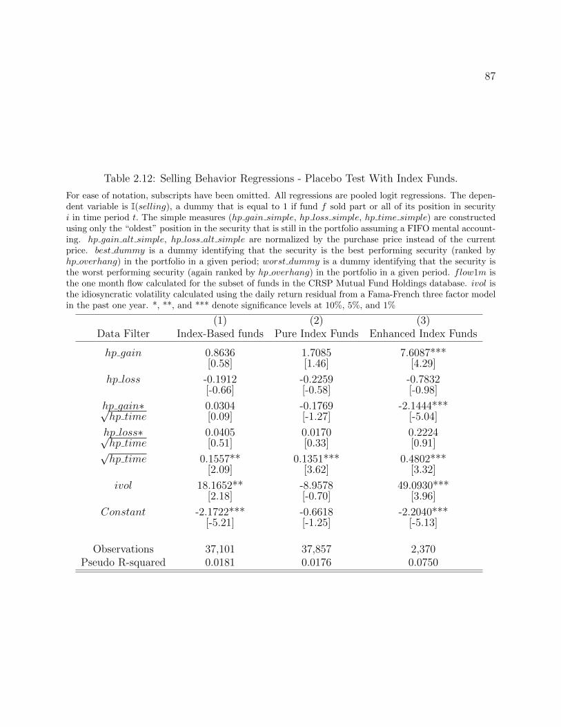
87

Table 2.12: Selling Behavior Regressions - Placebo Test With Index Funds.

For ease of notation, subscripts have been omitted. All regressions are pooled logit regressions. The depen-dent variable is I(selling), a dummy that is equal to 1 if fund f sold part or all of its position in securityi in time period t. The simple measures (hp gain simple, hp loss simple, hp time simple) are constructedusing only the “oldest” position in the security that is still in the portfolio assuming a FIFO mental account-ing. hp gain alt simple, hp loss alt simple are normalized by the purchase price instead of the currentprice. best dummy is a dummy identifying that the security is the best performing security (ranked byhp overhang) in the portfolio in a given period; worst dummy is a dummy identifying that the security isthe worst performing security (again ranked by hp overhang) in the portfolio in a given period. flow1m isthe one month flow calculated for the subset of funds in the CRSP Mutual Fund Holdings database. ivol isthe idiosyncratic volatility calculated using the daily return residual from a Fama-French three factor modelin the past one year. *, **, and *** denote significance levels at 10%, 5%, and 1%

(1) (2) (3)Data Filter Index-Based funds Pure Index Funds Enhanced Index Funds

hp gain 0.8636 1.7085 7.6087***[0.58] [1.46] [4.29]

hp loss -0.1912 -0.2259 -0.7832[-0.66] [-0.58] [-0.98]

hp gain∗ 0.0304 -0.1769 -2.1444***√hp time [0.09] [-1.27] [-5.04]

hp loss∗ 0.0405 0.0170 0.2224√hp time [0.51] [0.33] [0.91]√hp time 0.1557** 0.1351*** 0.4802***

[2.09] [3.62] [3.32]

ivol 18.1652** -8.9578 49.0930***[2.18] [-0.70] [3.96]

Constant -2.1722*** -0.6618 -2.2040***[-5.21] [-1.25] [-5.13]

Observations 37,101 37,857 2,370Pseudo R-squared 0.0181 0.0176 0.0750

Chapter 3

Mortgage Debt, Recourse, and

Strategic Default

Li An

89

3.1 Introduction

The most recent housing market downturn, which started in 2006, is one of the worst housing

crises in history. House prices plunged and defaults zoomed to historical highs around the

United States. In California, for example, the total number of strategic defaults was 68

times higher in 2008 than it was in 2005; in Florida, it was 46 times higher. In most other

parts of the country, defaults were about nine times higher in 2008 than in 20051. This crisis

is notable in that house prices have fallen by 40 to 50 percent during the last few years in

some areas, yet many home-owners owe more on their home mortgages than their houses

are worth because they put very little or nothing down when they bought their houses in

the expansion. Home-owners with a negative home equity have an incentive to strategically

default on their mortgage debt - render their houses to the bank and walk away, which the

Wall Street Journal calls ”American dream 2: default, then rent”2. Thus to reduce costly

default, it is important to understand the home-owners’ strategic default decision.

This paper explores how foreclosure legal arrangements have impacts on mortgage default

incentives and the mortgage market. In the literature, the lender’s claim in a mortgage

default is usually limited to the collateral, the house value, ever since Asay’s seminal effort

in 1978, which first applies the Black-Scholes (Black and Scholes 1972) option pricing model

to price mortgage. However, in many states in the United States, if the lender forecloses

1See Experian-Oliver Wyman, Market Intelligence Report, Understanding Strategic Default in Mortgages(2009)

2Wall Street Journal, 2009 December 16. ”American Dream 2: Default, Then Rent”.http://online.wsj.com/article/SB126040517376983621.html

90

and sells the house for less than the amount owed, the lender still has a recourse for the

difference. While this recourse decreases the payoff of strategic default, it raises debt value

ex ante, not only because it gives the creditor a greater claim in the state of default, but

also because it lowers the incentive for a strategic default. Indeed, in the past few years, the

default rate increased the most drastically in states,like California, where mortgage debt is

non-recourse and in states, like Florida, where legal restrictions and costs make the lender

very unlikely to collect on a deficiency judgement although foreclosure law allows recourse.

This paper provides a theoretical model that explicitly analyzes the strategic default

incentives under different foreclosure laws. I build the model based on the structural credit

risk framework by Leland (1994), who uses the option-based valuation technique to analyze

the problem of corporate bonds with endogenous default incentives. The relatively simple

framework allows me to reach a tractable closed-form solution.

In the baseline model, I discuss the situation in which a home-owner does not have any

cash flow problems, and strategic default is the only source of default. In the full model, I

include a liquidity shock to the home-owner who may have to default for cash flow reasons,

although he or she otherwise wants to keep serving the debt out of his or her financial

interest. The key results are that possible recourse makes the payoff in strategic default

less attractive, and it deters strategic default when the house price goes down. The full

model illustrates that liquidity shocks not only incur liquidity default, which is obvious

by definition, but they also exacerbate the strategic default problem since they lower the

continuation value:continue to severe the debt now involves a potential loss of value due to

91

possible liquidity default in the future. Recourse could help reduce default incentives and

make debt value immune to liquidity shock, and it has little impact on house equity value in

the presence of the interaction between cash flow problems and strategic default incentives.

The deterrent role of recourse is consistent with the empirical evidence found by Ghent and

Kudlyak (2009).

This paper also relates to the discussion on why ”so few” home-owners with negative

equity actually default, which contradicts the predictions of standard option-based default

models. Recent empirical evidence of the low numbers of defaults is reported by Guiso,

Sapienza, and Zingales(2009), Foote, Gerardi, and Willen (2008), and Experian and Oliver

Wyman (2009), while early theoretical and empirical results are summarized by Vandell

(1995). In light of this model, if there is recourse for the mortgage debt, the default boundary

of equity value is actually not zero, but rather a negative value that equals the value of the

obligation potentially in default. In an extreme case of full-recourse, this value could be as

low as -100% of the initial home equity, which suggests that a large difference may exist

between what is predicted by theory and what is measured empirically.

The paper is organized as follows. Section 3.2 provides a brief overview of the foreclosure

law across the states. Section 3.3 presents the baseline model. Section 3.4 presents the full

model with liquidity shock. Section 3.5 discusses the policy implications and concludes the

paper.

92

3.2 Foreclosure Law across the States

In the case of a mortgage default, if selling the house garners less than the amount of debt

owned by the borrower, the lender may or may not have recourse for the shortfall according

to foreclosure law. It is actually a unique phenomenon in the United States that mortgage

loans can be non-recourse in some states. Across states, the foreclosure laws vary a lot.

Some states explicitly classify mortgage loans as non-recourse, for instance, Arizona,

California, and Oregon, while most states allow deficiency judgment. Among the states

that allow the lender to pursue recourse, several aspects of recourse vary. First, different

restrictions exist on how the fair market value is determined. In some states, a single ap-

praiser determines the fair market value, while in other states a fair market value must be

determined by a jury; legal costs and time required in such a process also differ because

restrictions vary. Second, state foreclosure laws differ on whether a time-consuming judi-

cial foreclosure process is required to obtain the deficiency judgment. Third, the personal

property or wages that can be exempted from collection differs by state. The onerous time

and legal costs can make it impractical to pursue deficiency judgment, although it is legally

allowed. Ghent and Kudlyaky (2009) discuss foreclosure arrangements in details and they

also include a summary of foreclosure law by state in their appendix.

Even when deficiency judgment is obtained, the borrower still has the option to claim

personal bankruptcy. The claim on the shortfall is noncollateral and can be discharged in

bankruptcy.

93

3.3 The Baseline Model: Borrower without Cash Flow

Problems

3.3.1 Model Set-up

Assume the house price follows a continuous diffusion process with drift µ(V, t) and constant

proportional volatility σ,

dV

V= µ(V, t) dt+ σdZ

where dZ is an increment of standard Brownian motion.

A borrower (home-buyer) who wants to purchase a house at day zero, but is wealth-

constrained, must obtain funds from a bank. Assume the mortgage market is competitive,

banks are risk neutral, and the risk-free rate is r. The initial loan-to-value ratio a is deter-

mined by the initial financial condition of the borrower as well as his or her credit-worthiness

which limits the amount he or she can borrow; here I take a as given. In general, owning a

house has consumption value, the utility of living in the house, as well as asset value, the

gain (loss) from potential appreciation (depreciation) of the house price. The consumption

value could be achieved by renting a house with the money that would otherwise used in

house purchase or mortgage repayment; thus for simplicity, a home-owner in this model only

cares about the asset value, or to be more specific, the equity value of the house.

A mortgage contract between the borrower and the bank specifies:

A) Maturity T . In this model, I assume T =∞.

94

B) The principal M, which equals to loan-to-value ratio a times initial house value; that

is, M = aV

C) A fix-rate repayment schedule C. Fair price of initial mortgage rate would set the

value of newly made mortgage debt equal to the principal (D = M).

The payoffs to both parties in the case of mortgage default are governed by state fore-

closure law. In default, the house would be sold to repay the balance. In a fire sale or

costly foreclosure, only a fraction of current house value can typically be recovered; let α

denotes this fraction. As discussed in section 3.2, whether the lender has recourse in case of

default varies across states; in states that allow deficiency judgement, costs and restrictions

differ and affect the ease of obtaining recourse. I model the variation in legal arrangement

with a parameter β ∈ [0, 1], which denotes the probability of obtaining recourse. Finally,

the borrower also has the option to file personal bankruptcy after default on a mortgage,

which can discharge the claim over the shortfall. I denote the probability of bankruptcy

after deficiency judgement with 1− p; that is, there are chances that the borrower actually

pays back the difference.

In the baseline model, I assume the borrower does not have any cash flow problems -

he or she can keep serving the mortgage debt as long as he or she wants. The only case in

which default happens is when the house value drops too low and continuing to serve the

debt is worse than defaulting and facing a possible obligation on the shortfall. Of course,

in practice, besides the strategic default already mentioned, cases also exist in which the

borrower wants to serve the debt because it is best for his or her financial interest, but he

95

or she has cash flow problems and cannot meet the payment. I call the second kind liquidity

default, and I ’ll discuss the full model, taking both types into account, in section 4.

The overall expected payoff of the lender when the borrower defaults on mortgage is

αV + βp(M − αV )

Symmetrically, the boundary payoff for the borrower in default is

−βp(M − αV )

3.3.2 Valuation and Endogenous Default Boundary

Debt Value and Equity Value

As standard in Leland’s (1994) framework, when the house value V drops to a boundary VB,

the equity value drops to the continuation value, which equals the payoff in default. The

borrower would then declare default on the mortgage. We take this boundary as given for

now and will find the endogenous default boundary later.

We consider the value of this mortgage debt, D(V ;VB), which depends on current house

price V and the default boundary VB,. Since the maturity is infinity, debt value is time-

independent. As in Leland (1994), the debt value satisfies the following partial derivative

equation:

96

rD = rV DV +1

2σ2V 2DV V + C (3.1)

where DV and DV V are the first and second partial derivative of D with respect to V .

The left side of the equation is the required instantaneous return of the bond in a risk-

neutral world. And the right side is the instantaneous change of debt value due to the change

of the house value V (the first two terms), plus a coupon payment per unit of time.

We know PDE of this form has a general solution in the form of

D = A0 + A1V + A2V−X (3.2)

X =2r

σ2

Two boundary conditions:

D(VB) = αV + βp(M − αV )

D(∞) =C

r

set the debt value equal to the lender’s payoff in default when V hits the default boundary VB

, and equal to the value of the riskless perpetuity with coupon C as V goes toward infinity.

We solve for the coefficients in (2) by plugging in the two boundary conditions and get

D(V ;VB) =C

r+ [(1− βp)αVB + βpM − C

r)(V

VB)−X

97

Consider a claim that pays (1 − α)V only in default. Such a claim has the same value

as value loss in default, or the bankruptcy cost. The present value of such bankruptcy cost

BC(V ;VB) also satisfies equation (1) and has boundary conditions:

BC(VB) = (1− α)V

BC(∞) = 0

Thus

BC(V ;VB) = (1− α)VB(V

VB)−X

The equity value of the homeowner at any point of time is the current house value minus

the bankruptcy cost associated with borrowing, then minus the current value of the mortgage

debt. That is

E(V ;VB) = V −BC(V ;VB)−D(V ;VB)

= V − C

r+ [

C

r− (1− βpα)VB − βpM ](

V

VB)−X

Endogenous Default Boundary

Consider the home-buyer’s problem. Since he or she cannot commit to not strategically

default, and his or her equity value depends on the fair mortgage rate, which in turn depends

98

on the lender’s expectation of the home-buyer’s default choice. Therefore, in equilibrium,

the home-buyer would choose the default boundary that maximizes his or her equity value;

this is also fairly expected by the lender.

The first order condition is:

∂E(V ;VB)

∂VB= 0

we solve for the default boundary VB :

VB =X

(1− βpα)(1 +X)(C

r− βpM)

which does not depend on V.

Plug VB back into D(V ;VB) and E(V ;VB), and we have the following:

D(V ) =C

r− (1− βpα +X − αX)[

(Cr− βpM)

(1− βpα)(1 +X)]X+1(

V

X)−X

E(V ) = V − C/r + (1− βpα)[(Cr− βpM)

(1− βpα)(1 +X)]X+1(

V

X)−X

3.3.3 Results: Recourse, Strategic Default and Mortgage Market

To answer the question of what effect the legal environment has on mortgage default and

mortgage market, I first show that the probability of obtaining recourse affects debt value,

not only by increasing the lender’s or debt holders’ payoff in default, but also by influencing

99

strategic default incentives. I then discuss the effect on the mortgage debt market.

The discussion is made under the following set of baseline parameters:

r = 3%

σ = 5%

α = 0.7

p = 0.5

a = 80%

V0 = 100

I set the annual risk-free rate r to be 3%, and the annual volatility of house prices σ to

be 5%, which is consistent with empirical facts. Proportion of value recovered in fire sale or

foreclosure α is set as 0.7; this is consistent with the estimation made by Campbell, Giglio

and Pathak (2009), who find foreclosure reduces the value of the home by approximately

28%. I let the probability of personal bankruptcy after deficiency judgment p to be 0.5,

initial loan to value ratio a to be 80%, and initial value of a house V0 to be 100. Thus the

initial mortgage loan balance M is 80 and the book value of equity is 20.

Fix-rate coupon C is such that the initial debt value is at par. I choose the smallest

positive real root of equation D(V0;C) = M to be C. Initial mortgage rate, the one in the

100

mortgage contract, is calculated as R = CM

; mortgage yield, the bond yield in the second

market, is calculated as y = CD(V )

, which changes with the house value.

Negative Equity, Strategic Default, and Foreclosure Law

The recent housing crisis has attracted the attention of many economists trying to under-

stand home-owners’ mortgage default decisions. Among other works, Guiso, Sapienza, and

Zingales (2009) study survey data and find that no household would default if the equity

shortfall is less than 10% of the house value; 17% of households would default, even if the

home-owners can afford to pay their mortgage, if the equity shortfall reaches 50% of their

house value. Many people are puzzled by so few home-owners defaulting when the value of

their house is less than the mortgage balance because it contradicts the economic rationale.

Guiso, Sapienza and Zingales (2009) explain this outcome as arising from moral and social

constraints. I argue that transaction costs, which include moving costs, sentimental attach-

ment to the house, reputation issues, and moral concerns, and so forth, are important in

practice; however, it may not be necessary to turn to transaction costs to explain the low

number of defaults on negative equity houses. Several points exist that may give more power

to the ”ruthless” economic theory.

First, the economic value of equity may disagree with the book value of equity, which

is typically used in empirical works. Economic value of equity is larger than book value,

since it contains the option value of default later. Or from another perspective, equity value

equals house value less debt value and the present value of bankruptcy cost; when house

101

price falls, debt value would be significantly reduced from par value. Thus, when the book

value of house equity drops to zero, economic value could still be positive. Similar arguments

are made by Foote, Gerardi, Paul, and Willen (2008).

Second, when a lender could possibly obtain recourse over the difference between debt

balance and proceeding, the alternative value of default is the probability of obtaining re-

course times the shortfall of the amount owned, which is no longer zero. In other words,

violation of limited obligation makes the alternative choice of default worse; thus, the eq-

uity value at which the borrower would choose to default falls accordingly. The greater the

probability that deficiency judgment will be achieved, the worse the payoff to borrower in

default, and thus the more effective deterrent role that foreclosure law plays.

Figure 3.1 illustrates the effect of legal environment on a borrower’s default incentive.

Panel A shows the default boundary falling from 77, which is close to the book value of 80,

to 59, as the probability of obtaining a deficiency judgment increases from 0 to 1. Panel B

plots the initial value of equity when house value V=100; when the probability of obtaining

a deficiency judgment is high (close to 1), the house equity is almost equal to the book value,

and there is almost no loss of value due to potential bankruptcy. This is consistent with

the empirical results of Ghent and Kudlyak (2009) who find that at the mean value of the

default option at the time of default, the probability of default is 20% higher in non-recourse

states than in recourse states.

The relationship between house equity value and strategic default is more clearly illus-

trated in Figure 3.2. As the house price falls from 100 to 60, the house equity value falls

102

Figure 3.1: Default Boundary, House Equity Value and Recourse.

(a) Panel A

0 0.2 0.4 0.6 0.8 158

60

62

64

66

68

70

72

74

76

78

probability of deficiency judgement beta

bank

rupt

cy b

ound

ary

VB

(b) Panel B

0 0.2 0.4 0.6 0.8 1

19.96

19.965

19.97

19.975

19.98

19.985

19.99

19.995

20

20.005


init

ial e

quit

y va

lue

accordingly. The four vertical lines plot the default boundary when the book value of equity

and the economic value are considered, while the probability of obtaining a deficiency judg-

ment β equals 0, 0.5 and 1, respectively. First, when the book value of equity drops to zero

(i.e. V = 80), the value of equity is above zero when β = 0, although the difference is not

large, which suggests that book value of equity is not a bad proxy when mortgage debt is

non-recourse. However, when the probability of obtaining a deficiency judgment increases to

0.5 and 1, the equity values at which default happens are about −40% and −100% of book

equity. This may help to explain why many people keep serving the debt while (the book

value of) house equity is significantly negative, without turning to transaction costs.

103

Figure 3.2: House Equity Value When House Price Falls

556065707580859095100-20

-15

-10

-5

0

5

10

15

20

house price V

equi

ty v

alue

VB whenbeta=0

book value=0

VB whenbeta=0.5

VB whenbeta=1

beta=0

beta=0.5

beta=1

Mortgage Debt Market and Foreclosure Law

Home-owners’ default decisions directly affect the mortgage debt market, which is in turn

closely related to foreclosure law. Figure 3.3 shows how debt value changes under a different

legal environment when a house price falls. On the left side, where mortgage debt is non-

recourse, debt value is sensitive to changes in house price - debt value decreases 12.5% in

response to a 20% drop in house price, when initial loan-to-value ratio(LTV) is 80% as

specified above. In contrast, on the right side, where mortgage debt has full recourse, debt

value is almost unaffected by the fluctuation in house price.

104

Figure 3.3: Debt Value When House Price Falls.

0 0.2 0.4 0.6 0.8 170

72

74

76

78

80

82


debt

val

ue

V=80

V=90

V=100

Foreclosure law affects payoffs and strategic default incentives ex post, as well as the

expectation of default ex ante. Figure 3.4 plots the ex ante mortgage rate, which sets the

initial debt value to book value, and the ex post mortgage yield when V=80 against β. Note

that the spread over risk-free rate is small in both cases. This is because the model assumes

infinite maturity, thus the present value is very sensitive to change in discount rate. A very

slight change in mortgage rate would result in a large variation of debt value. Nevertheless,

mortgage rate and mortgage yield are qualitatively more volatile when mortgage debt is

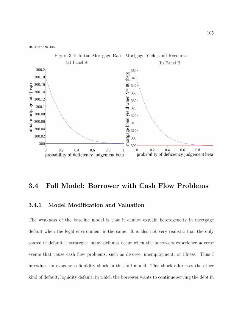
105

non-recourse.

Figure 3.4: Initial Mortgage Rate, Mortgage Yield, and Recourse.

(a) Panel A

0 0.2 0.4 0.6 0.8 1

300

300.02

300.04

300.06

300.08

300.1

300.12

300.14

300.16

300.18

300.2


init

ial m

ortg

age

rate

(bs

p)

(b) Panel B

0 0.2 0.4 0.6 0.8 1300

305

310

315

320

325

330

335

340

345

350


mor

tgag

e bo

nd y

ield

whe

n V

= 8

0 (b

sp)

3.4 Full Model: Borrower with Cash Flow Problems

3.4.1 Model Modification and Valuation

The weakness of the baseline model is that it cannot explain heterogeneity in mortgage

default when the legal environment is the same. It is also not very realistic that the only

source of default is strategic: many defaults occur when the borrowers experience adverse

events that cause cash flow problems, such as divorce, unemployment, or illness. Thus I

introduce an exogenous liquidity shock in this full model. This shock addresses the other

kind of default, liquidity default, in which the borrower wants to continue serving the debt in

106

his or her financial interest, but has to default because he or she cannot meet the payment

for cash flow reasons. This liquidity shock can be interpreted as reflecting heterogeneous

characteristics of the borrower because it depends on personal income, creditability, and so

forth. It can also be interpreted on an aggregate level as changes in the economic situation.

I model this liquidity shock with parameter l ∈ [0, 1], the arrival rate of the liquidity

shock that causes the borrower fail to keep making mortgage payment. All other conditions

are as specified in the model set-up in section 3.3. I solve the equity value directly by solving

rE = rV EV +1

2σ2V 2EV V − C − l[E −max(αV −M, 0)− βpmax(M − αV, 0)]

The left side is the required instantaneous return of the equity in a risk-neutral world.

On the right side, the first two terms are the instantaneous change of equity value due to the

change of house value V, the third term is coupon payment per unit of time, and the fourth

term is the instantaneous expected value loss to a home-owner due to liquidity shock. When

the liquidation value αV is greater than balance M , the payoff to the home owner in liquidity

default is αV −M ; when the liquidation value αV is less than balance M , the payoff to the

home owner is the possible claim over the shortfall βp(M−αV ); and the expected loss is the

difference between the current equity value and the terminal payoff times the arrival rate l.

107

Boundary conditions are:

E(VB;VB) = −βp(M − αV )

E(V ;VB) |V→∞ = V − C

r

where VB = arg maxVb

E(V ;Vb)

Symmetrically, debt value satisfies the equation:

rD = rV DV +1

2σ2V 2DV V + C − l[D −min(M,αV + βpmax(M − αV, 0)]

The last term on the right side indicates that the expected loss due to liquidity shock is

l times the difference between current debt value D and the the terminal payoff in liquidity

default; that is M when M < αV , and αV + βp(M − αV ) when M > αV . Boundary

conditions are

D(VB) = αV + βp(M − αV )

D(∞) =C

r

I solve this model numerically, under the baseline parameter values as previously specified.

108

3.4.2 Results: Recourse, Liquidity Shock and Mortgage Default

In this section I discuss the effect of a liquidity shock on mortgage default incentive and

mortgage market under different legal environments. The unexpected feature means the liq-

uidity shock is not priced in the coupon payment, and it captures an unexpected change in

the home-owner’s financial condition. Several interpretations are possible. First, a liquidity

shock can be interpreted as an unexpected deterioration of an individual’s situation, which is

independent across borrowers. As emphasized in Capozza, Kazarian, and Thomson (1997),

adverse events such as divorce, illness, and unemployment play important roles in mortgage

default. Second, a liquidity shock can also be interpreted as an unexpected economic down-

turn, such as the current financial crisis, in which unemployment rate surges, asset prices

plunge, and the current and expected future cash flows of all individuals in the economy are

adversely affected.

Figure 3.5 plots the relationship between default boundary VB and probability of defi-

ciency judgment β under different arrival rates of liquidity shock l. The plot clearly shows

that liquidity shock increases mortgage default rate, not only because it affects borrowers’

ability to pay, but less evidently, because it also affects borrowers’ incentive to pay. As the

arrival rate increases, it is less attractive for a borrower to keep serving the debt. Since

the continuation value decreases, it is more likely in the future that a liquidity shock would

occur in which case the borrower has to bear the loss in liquidity default. He or she would

thus default at a house value at which she would not have before. And this strategic de-

109

fault incentive is exacerbated by lack of recourse - the lower the probability of obtaining a

deficiency judgment, the higher the default boundary.

Figure 3.5: Default Boundary in Presence of Liquidity Shock.

0 0.2 0.4 0.6 0.8 160

65

70

75

80

85

90

probability of deficiency judgement

defa

ult b

ound

ary

VB

l=1%

l=0.5%

l=0%

Figure 3.6 plots the debt and equity value when V=100. Panel A shows that debt value is

very sensitive to liquidity shock when β is small, while it is almost unaffected when β is large.

In contrast, as shown in panel B, β has little impact on equity value under any of the three

scenarios. This suggests that greater recourse could help increase debt value by deterring

strategic default and avoiding bankruptcy cost, while also not decreasing a home-owner’s

value too much.

110

Figure 3.6: Debt Value and Equity Value in Presence of Liquidity Shock When V=100.

(a) Panel A

0 0.2 0.4 0.6 0.8 171

72

73

74

75

76

77

78

79

80

81


debt

val

ue w

hen

V=

100

l=0%

l=0.5%

l=1%

(b) Panel B

0 0.2 0.4 0.6 0.8 18

10

12

14

16

18

20


equi

ty v

alue

whe

n V

=10

0

l=0%

l=0.5%

l=1%

Mortgage bond values are adversely affected in recessions in which people have more cash

flow problems, and the mortgage bond spread widens. The 2008 financial crisis showed the

mortgage spread surged to a historical high. Figure 3.7 plots the debt value and mortgage

bond yield when V = 90, a 10% drop in house price. When mortgage debt is non-recourse,

debt value could be largely affected by changes in the house price, in the presence of liquidity

shock, and mortgage bond market could be very volatile. In contrast, full recourse makes

debt value immune to changes in the house price even when liquidity shock is relatively high.

111

Figure 3.7: Debt Value and Mortgage Yield in Presence of Liquidity Shock When V=90.

(a) Panel A

0 0.2 0.4 0.6 0.8 1-10

0

10

20

30

40

50

60

70

80


debt

val

ue w

hen

V=

90

l=0%

l=0.5%

l=1%

(b) Panel B

0 0.2 0.4 0.6 0.8 1300

500

700

900

1100


mor

tgag

e yi

eld

whe

n V

=90

(bs

p)

l=0%

l=0.5%

l=1%

3.5 Policy Implications and Conclusions

One important policy question in the most recent housing crisis is how to reduce foreclosure.

As reported in many recent empirical studies, strategic default has become a severe problem

because house prices have fallen in the last few years by 40 to 50 percent in some areas. Many

borrowers had put very little down when they bought their houses, which is historically a

rare case. Thus a policy that aims at alleviating the situation should effectively address the

default incentive issues.

The two common loss mitigation policies are modification and forbearance. Modification

involves permanent changes in the original terms on the loan, while forbearance allows the

lender to temporarily forebear the low payment or late payment, without changing the

112

initial terms. Under the framework of this model, the modification may help those who are

experiencing cash flow problems, but it does not work for strategic defaults because it does

not affect default incentives. This explain the concern of Adelino, Gerardi and Willen (2009)

about re-default issues. On the other hand, forbearance would mitigate the situation becuase

it reduces liquidity defaults. More importantly, however, it can increase the continuation

value of serving the debt by decreasing the probability that a liquidity shock occurs and the

borrower has to default; thus strategic default boundary should fall as well.

This paper analyzes the strategic default problem using an option-based model, and

shows that recourse can play an effective role in deterring default when a house price falls

or the economic situation goes bad. It reduces strategic default by diminishing the payoff in

default, thus it makes continuing to serve the debt the more economical choice. In addition

to popular policies, this paper suggests that recourse might be another possible solution to

the default problem. The caveat is that, deterring defaults will adversely affect the welfare

of home-buyers who are in really bad situations; to make a feasible policy, home-buyers need

to be compensated through other channels, which needs further studies in the future.

Bibliography

Adelino, Manuel, Kristopher Gerardi and Paul S. Willen. 2013. “Why don’t Lenders renegoti-ate more home mortgages? Redefaults, self-cures and securitization.” Journal of MonetaryEconomics 60(7):835–853.URL: http://www.sciencedirect.com/science/article/pii/S0304393213001086

An, Li. 2014. “Asset Pricing when Traders Sell Extreme Winners and Losers.” ColumbiaUniversity Working Paper .URL: http://papers.ssrn.com/abstract=2355520

Ang, Andrew, Robert Hodrick, Yuhang Xing and Xiaoyan Zhang. 2006. “The Cross-Sectionof Volatility and Expected Returns.” The Journal of Finance 61(1):259–299.

Ang, Andrew, Robert Hodrick, Yuhang Xing and Xiaoyan Zhang. 2009. “High Idiosyn-cratic Volatility and Low Returns: International and Further U.S. Evidence.” Journal ofFinancial Economics 91(1):1–23.

ANTON, MIGUEL and CHRISTOPHER POLK. 2014. “Connected Stocks.” The Journalof Finance 69(3):1099–1127.URL: http://doi.wiley.com/10.1111/jofi.12149

Argyle, Bronson. 2013. “Portfolio Spillovers and a Limit to Diversification.” Columbia Uni-versity Working Paper .URL: http://papers.ssrn.com/abstract=2343149

Asay, Michael. 1978. Rational Mortgage Pricing. PhD thesis University of Southern Califor-nia.

Asparouhova, Elena, Hendrik Bessembinder and Ivalina Kalcheva. 2010. “Liquidity biasesin asset pricing tests.” Journal of Financial Economics 96(2):215–237.

Barber, Brad and Terrance Odean. 2013. The Behavior of Individual Investors. In Handbookof the Economics of Finance, ed. George Constantinides, Milton Harris and Rene Stulz. 1ed. Vol. 2 North Holland pp. 1533–1570.

113

114

Barberis, Nicholas and Wei Xiong. 2009. “What Drives the Disposition Effect? An Analysisof a Long-Standing Preference-Based Explanation.” the Journal of Finance 64(2).

Barberis, Nicholas and Wei Xiong. 2012. “Realization utility.” Journal of Financial Eco-nomics 104(2):251–271.

Ben-David, Itzhak and David Hirshleifer. 2012. “Are Investors Really Reluctant to RealizeTheir Losses? Trading Responses to Past Returns and the Disposition Effect.” Review ofFinancial Studies 25(8):2485–2532.

Birru, Justin. 2012. “Confusion of confusions: A test of the disposition effect on momentum.”Working Paper, Fisher College of Business, Ohio State University .

Black, Fischer and Myron S Scholes. 1973. “The Pricing of Options and Corporate Liabili-ties.” Journal of Political Economy 81(3):637–54.URL: http://ideas.repec.org/a/ucp/jpolec/v81y1973i3p637-54.html

Blocher, Jesse. 2011. “Contagious capital: A network analysis of interconnected intermedi-aries.” Available at SSRN 1968488 .URL: http://papers.ssrn.com/sol3/papers.cfm? abstract id=1968488.

Bollen, Nicolas P. B. and Jeffrey A. Busse. 2001. “On the Timing Ability of Mutual FundManagers.” The Journal of Finance 56(3):1075–1094.URL: http://doi.wiley.com/10.1111/0022-1082.00356

Busse, J. A. 1999. “Volatility timing in mutual funds: evidence from daily returns.” Reviewof Financial Studies 12(5):1009–1041.URL: http://rfs.oxfordjournals.org/content/12/5/1009.short

Camerer, Colin and Martin Weber. 1998. “The disposition effect in securities trading: anexperimental analysis.” Journal of Economic Behavior & Organization 33(2):167–184.

Capozza, Dennis R., Dick Kazarian and Thomas A. Thomson. 1997. “Mortgage Default inLocal Markets.” Real Estate Economics 25(4):631–655.URL: http://doi.wiley.com/10.1111/1540-6229.00731

Carhart, Mark. 1997. “On persistence in mutual fund performance.” The Journal of finance52(1):57–82.URL: http://onlinelibrary.wiley.com/doi/10.1111/j.1540-6261.1997.tb03808.x/full

Chevalier, Judith and Glenn Ellison. 1997. “Risk Taking by Mutual Funds as a Response toIncentives.” Journal of Political Economy 105(6):1167–1200.URL: http://ideas.repec.org/a/ucp/jpolec/v105y1997i6p1167-1200.html

115

Choi, Wonseok, Kenton Hoyem and Jung-Wook Kim. 2008. “Not All Trading Volumesare Created Equal: Capital Gains Overhang and the Earnings Announcement VolumePremium.” Available at SSRN: http://ssrn.com/abstract=1140743 .

Cochrane, John. 2011. “Presidential address: Discount rates.” The Journal of Finance66(4):1047–1108.URL: http://onlinelibrary.wiley.com/doi/10.1111/j.1540-6261.2011.01671.x/full

Coval, Joshua and Erik Stafford. 2007. “Asset fire sales (and purchases) in equity markets.”Journal of Financial Economics 86(2):479–512.URL: http://dx.doi.org/10.1016/j.jfineco.2006.09.007 http://linkinghub.elsevier.com/retrieve/pii/S0304405X07001158http://www.sciencedirect.com/science/article/pii/S0304405X07001158

Coval, Joshua and Tyler Shumway. 2005. “Do Behavioral Biases Affect Prices?” The Journalof Finance 60(1):1–34.

Daniel, Kent, Mark Grinblatt, Sheridan Titman and Russ Wermers. 1997. “Measuringmutual fund performance with characteristic-based benchmarks.” The Journal of Finance52(3):1035–1058.

Daniel, Kent and Sheridan Titman. 2006. “Market Reactions to Tangible and IntangibleInformation.” The Journal of Finance 61(4):1605–1643.

De Bondt, Werner and Richard Thaler. 1985. “Does the Stock Market Overreact?” TheJournal of Finance 40(3):793–805.

Fama, Eugene and James MacBeth. 1973. “Risk, Return, and Equilibrium: Empirical Tests.”Journal of Political Economy 81(3):607–636.

Fama, Eugene and Kenneth French. 1993. “Common risk factors in the returns on stocksand bonds.” Journal of Financial Economics 33(1):3–56.

Feng, Lei and Mark Seasholes. 2005. “Do Investor Sophistication and Trading ExperienceEliminate Behavioral Biases in Financial Markets?” Review of Finance 9(3):305–351.

Foote, Christopher L., Kristopher Gerardi and Paul S. Willen. 2008. “Negative equity andforeclosure: Theory and evidence.” Journal of Urban Economics 64(2):234–245.URL: http://www.sciencedirect.com/science/article/pii/S0094119008000673

Frazzini, Andrea. 2006. “The disposition effect and underreaction to news.” The Journal ofFinance 61(4):2017–2046.

Genesove, David and Christopher Mayer. 2001. “Loss aversion and seller behavior: Evidencefrom the housing market.” The Quarterly Journal of Economics 116(4):1233–1260.

116

Gervais, Simon, Ron Kaniel and Dan Mingelgrin. 2001. “The High-Volume Return Pre-mium.” The Journal of Finance 56(3):877–919.

Ghent, Andra C. and Marianna Kudlyak. 2011. “Recourse and Residential Mortgage Default:Evidence from U.S. States.” SSRN Electronic Journal 24(9):3139 – 3186.URL: http://www.ssrn.com/abstract=1432437

Goetzmann, William and Massimo Massa. 2008. “Disposition matters: volume, volatilityand price impact of a behavioral bias.” Journal of Portfolio Management 34(2):103–25.

Grinblatt, Mark and Bing Han. 2005. “Prospect theory, mental accounting, and momentum.”Journal of financial economics 78(2):311–339.

Grinblatt, Mark and Matti Keloharju. 2001. “What makes investors trade?” The Journalof Finance LVI(2):589–616.URL: http://www.blackwell-synergy.com/doi/abs/10.1111/0022-1082.00338

Grinblatt, Mark, Matti Keloharju and Juhani Linnainmaa. 2012. “IQ, trading behavior, andperformance.” Journal of Financial Economics 104(2):339–362.

Guiso, Luigi, Paola Sapienza and Luigi Zingales. N.d. “Moral and Social Constraints toStrategic Default on Mortgages.” NBER Working Papers. Forthcoming.URL: http://ideas.repec.org/p/nbr/nberwo/15145.html

Hartzmark, Samuel M. 2013. “The Worst, the Best, Ignoring All the Rest: The Rank Effectand Trading Behavior.” Working paper, University of South California .

Heath, Chip, Steven Huddart and Mark Lang. 1999. “Psychological Factors And StockOption Exercise.” The Quarterly Journal of Economics 114(2):601–627.

Hong, Harrison, Terence Lim and Jeremy Stein. 2000. “Bad news travels slowly: Size, analystcoverage, and the profitability of momentum strategies.” The Journal of Finance 55(1).

Israel, Ronen and Tobias J. Moskowitz. 2013. “The role of shorting, firm size, and time onmarket anomalies.” Journal of Financial Economics 108(2):275–301.

Jegadeesh, Narasimhan. 1990. “Evidence of Predictable Behavior of Security Returns.” TheJournal of Finance 45(3):881–898.

Jegadeesh, Narasimhan and Sheridan Titman. 1993. “Returns to Buying Winners and SellingLosers: Implications for Stock Market Efficiency.” The Journal of Finance 48(1):65–91.

Kahneman, Daniel and Amos Tversky. 1979. “Prospect Theory: An Analysis of Decisionunder Risk.” Econometrica 47(2):263–91.

117

Lee, Charles and Bhaskaran Swaminathan. 2000. “Price Momentum and Trading Volume.”The Journal of Finance 55(5):2017–2069.

Locke, Peter and Steven Mann. 2005. “Professional trader discipline and trade disposition.”Journal of Financial Economics 76(2):401–444.

Lou, D. 2012. “A Flow-Based Explanation for Return Predictability.” Review of FinancialStudies 25(12):3457–3489.URL: http://rfs.oxfordjournals.org/content/early/2012/10/08/rfs.hhs103.full

Market Intelligence Report, Understanding Strategic Default in Mortgages. 2009. Technicalreport Experian-Oliver Wyman.

Novy-Marx, Robert. 2012. “Is momentum really momentum?” Journal of Financial Eco-nomics 103(3):429–453.

Odean, Terrance. 1998. “Are Investors Reluctant to Realize Their Losses ?” Journal ofFinance 53(5):1775–1798.

Seru, Amit, Tyler Shumway and Noah Stoffman. 2009. “Learning by Trading.” Review ofFinancial Studies 23(2):705–739.

Shapira, Zur and Itzhak Venezia. 2001. “Patterns of behavior of professionally managed andindependent investors.” Journal of Banking & Finance 25(8):1573–1587.

Shefrin, Hersh and Meir Statman. 1985. “The Disposition to Sell Winners Too Early andRide Losers Too Long: Theory and Evidence.” The Journal of Finance 40(3):777–790.

Shleifer, Andrei and Robert W. Vishny. 1997. “The Limits of Arbitrage.” The Journal ofFinance 52(1):35–55.URL: http://doi.wiley.com/10.1111/j.1540-6261.1997.tb03807.x

Shumway, Tyler and Guojun Wu. 2007. “Does disposition drive momentum.” Working Paper,University of Michigan .

Vandrell, Kerry. 1994. How ruthless is mortgage default? : a review and synthesis of theevidence. Madison: University of Wisconsin–Madison Center for Urban Land EconomicsResearch.

Wermers, Russ. 2004. “Is Money Really ’Smart’? New Evidence on the Relation BetweenMutual Fund Flows, Manager Behavior, and Performance Persistence.” Working Paper,University of Maryland .

Zuchel, Heiko and Martin Weber. 2002. “The Disposition Effect and Momentum.” Sonder-forschungsbereich 504 Publications, 01-26, Universitat Mannheim .

essays in investor behavior and asset pricing

Documents