three essays on pricing and hedging in incomplete...
TRANSCRIPT

Three Essays on Pricing and Hedging inIncomplete Markets
A thesis presented by
Dan Chen
London, October 19, 2011
Submitted for the for the degree of Doctor of Philosophy in the subject of Statistics,
London School of Economics and Political Science.

ii

Acknowledgement
I would like to thank Dr. Thorsten Rheinländer for his support and encouragement
throughout my master and PhD study. I cannot complete this dissertation without
his original ideas and technical advices. I also would like to thank him for the research
assistant position funded by the EPSRC grant.
My thanks also goes to Prof. Qiwei Yao, Dr. Kostas Kalogeropoulos, Sujin Park,
Hongbiao Zhao, Roy Rosemarin and many other people from the Statistics Depart-
ment for discussions and suggestions on my research. I also appreciate the improve-
ment advices from my two examiners, Prof. Dr. Rüdiger Kiesel and Dr. Angelos
Dassios.
The funding from the department made it is possible for me to live in London
independently and thus is greatly appreciated.
The biggest thanks, however, goes to my parents for their support, understanding
and encouragement.
iii

iv
Abstract
The thesis focuses on valuation and hedging problems when the market is incomplete.
The first essay considers the quadratic hedging strategy. We propose a generalized
quadratic hedging strategy which can balance a short-term risk (additional cost) with
a long-term risk (hedging errors). The traditional quadratic hedging strategies, i.e.
self-financing strategy and risk-minimization strategy, can be seen as special cases of
the generalized quadratic hedging strategy. This is applied to the insurance derivatives
market.
The second essay compares parametric and nonparametric measure-changing tech-
niques. The essay discusses three pricing approaches: pricing via Esscher measure,
via calibration and via nonparametric risk-neutral density; and empirically compares
the performance of the three approaches in the metal futures markets.
The last essay establishes the concept of stochastic volatility of volatility and
proposes several estimation methods.
v

vi

Contents
1 Introduction 1
1.1 Financial Mathematics and Financial Markets . . . . . . . . . . . . . . 1
1.1.1 Insurance derivatives . . . . . . . . . . . . . . . . . . . . . . . . 1
1.1.2 Metal futures . . . . . . . . . . . . . . . . . . . . . . . . . . . . 2
1.1.3 Equity and volatility derivatives . . . . . . . . . . . . . . . . . 3
1.2 Hedging in an incomplete market . . . . . . . . . . . . . . . . . . . . . 3
1.2.1 Dynamic quadratic hedging strategies . . . . . . . . . . . . . . 3
1.2.2 Other hedging strategies . . . . . . . . . . . . . . . . . . . . . . 4
1.3 Pricing in an incomplete market . . . . . . . . . . . . . . . . . . . . . 5
2 Generalized Quadratic Hedging Strategies 9
2.1 Introduction . . . . . . . . . . . . . . . . . . . . . . . . . . . . . . . . . 9
2.2 Quadratic hedging strategies for payment streams . . . . . . . . . . . . 10
2.3 Generalised quadratic hedging strategy . . . . . . . . . . . . . . . . . . 12
2.4 An example of a hedging annuity portfolio . . . . . . . . . . . . . . . . 16
2.4.1 Annuity portfolio . . . . . . . . . . . . . . . . . . . . . . . . . . 17
2.4.2 Mortality forward . . . . . . . . . . . . . . . . . . . . . . . . . 18
2.4.3 Hedging strategies and remaining risks . . . . . . . . . . . . . . 18
2.4.4 Numerical analysis . . . . . . . . . . . . . . . . . . . . . . . . . 20
2.5 Conclusion . . . . . . . . . . . . . . . . . . . . . . . . . . . . . . . . . 29
3 Risk-Neutral Densities and Metal Futures 33
3.1 Introduction . . . . . . . . . . . . . . . . . . . . . . . . . . . . . . . . . 33
3.2 Method1: price commodity futures under the Esscher measure . . . . 34
1
2 CONTENTS
3.2.1 Dynamics for the commodity spot prices . . . . . . . . . . . . . 34
3.2.2 Risk-neutral distribution estimated from spot price data . . . . 36
3.2.3 Futures price under the Esscher measure . . . . . . . . . . . . . 37
3.3 Method 2: model spot prices under the risk-neutral measure Q . . . . 40
3.4 Method 3: non-parametric estimation of risk-neutral densities . . . . . 41
3.5 Empirical analysis . . . . . . . . . . . . . . . . . . . . . . . . . . . . . 42
3.5.1 Estimation method and simulation techniques . . . . . . . . . . 42
3.5.2 Gold and gold future market . . . . . . . . . . . . . . . . . . . 44
3.5.3 Copper and copper future market . . . . . . . . . . . . . . . . . 52
3.5.4 Aluminum and aluminum future market . . . . . . . . . . . . . 58
3.6 Conclusion . . . . . . . . . . . . . . . . . . . . . . . . . . . . . . . . . 65
4 Stochastic Volatility of Volatility 69
4.1 Introduction . . . . . . . . . . . . . . . . . . . . . . . . . . . . . . . . . 69
4.2 The Concept of Volatility of Volatility . . . . . . . . . . . . . . . . . . 71
4.3 Stochastic Volatility of Volatility Model and Estimation Methods . . . 73
4.3.1 Bayesian MCMC . . . . . . . . . . . . . . . . . . . . . . . . . . 74
4.3.2 Maximum likelihood estimation via closed-form likelihood ex-
pansion . . . . . . . . . . . . . . . . . . . . . . . . . . . . . . . 81
4.3.3 Calibration . . . . . . . . . . . . . . . . . . . . . . . . . . . . . 83
4.4 Conclusion . . . . . . . . . . . . . . . . . . . . . . . . . . . . . . . . . 87

Chapter 1
Introduction
1.1 Financial Mathematics and Financial Markets
Earlier works in financial mathematics (Black and Scholes (1973), Merton (1973),
etc.) are based on the strong assumption that the market is complete, i.e. that all
contingent claims are replicable by investing in the underlying asset.
However, empirical studies suggest that the market is not complete in practice due
to various reasons like illiquidity, stochastic volatility or jumps in price processes [6].
Once we remove the completeness assumption, we have to face a so-called incomplete
market. In such markets, the pricing by replication is not working so optimal pricing
and hedging depend on the criteria chosen.
Before going into the details of pricing and hedging strategies designed for incom-
plete markets, we would like to introduce the financial markets that will be studied
later on.
1.1.1 Insurance derivatives
Insurance-linked securities have been used as a tool to transfer insurance risks from the
insurance industry to the capital market. At the same time, they provide the financial
market with a diversification tool, since insurance risks are often uncorrelated with
existing financial risks. According to Barrieu and Albertini (2009) [1], there were
approximately $13bn of tradable non-life insurance-linked securities and $24bn in
tradable life insurance-linked securities by the end of 2008.
The most successful non-life insurance-linked security is the catastrophe bond (cat
bond). A cat bond can be understood as an ’insurance contract’with the insurance
or reinsurance companies as the insured and capital market investors as the insurer.
The investors can receive interest payments and get back the principal as long as the
natural disaster does not occur before the maturity of the bond. More details about
cat bonds and other non-life insurance-linked securities can be found in [1].
Life insurance-linked securities include longevity bonds, survivor swaps, mortality
1

2 CHAPTER 1. INTRODUCTION
forwards etc. The typical underlying risks are mortality and longevity risk. Mortality
risk indicates the risk that the actual death rate exceeds the expected rate, whereas
longevity risk is the risk that the actual mortality becomes lower than expected.
Clearly there are plenty of organizations, such as pension funds and life-insurance
companies, which have exposures to mortality risk or longevity risk. Therefore they
are natural players in the life insurance-linked securities market. Capital market
speculators, like hedge funds, have also entered this market to diversify their portfolio
or earn speculating returns.
Insurance derivatives markets are in general incomplete due to illiquidity and basis
risks. The basis risks arise from the inconsistency between the underlying insurance
risk of the derivatives and the insurance risk of the hedger. For instance, an annuity
portfolio can have exposure to the longevity risks of a certain group of people in
England, but the tradable life-insurance derivatives, which the portfolio manager can
choose as hedging instruments, are based on nationwide mortality rates.
1.1.2 Metal futures
Metal futures markets have a long history and are in general mature markets. Precious
metal futures like gold are traded on Commodity Exchange, Inc. (COMEX) and lots
of local exchanges. Industrial metal futures, like copper, aluminium, zinc, etc. are
traded on London Metal Exchange (LME), COMEX, Shanghai Future Exchange, etc.
At a certain time point, we have a futures price curve consisting of spot price and
prices of futures with different maturities. We can describe the curve to be normal if
it is upward sloping over different maturities (starting with time 0) and to be inverted
if it is downward sloping. When we look at the evolvement of the futures price over
time, we will find that it will converge to the spot price when closer to the maturity.
We call the market is contango when the futures price is expected to decrease over
time to the futures spot price, and call the market is normal backwardation if the
futures price is expected to increase to the futures spot price as time goes by. (See
[27] for more details)
Unlike financial assets such as stock and bond, commodities can be consumed.
Moreover, it is sometimes beneficial to hold the commodity rather than the derivatives,
especially when the futures curve is inverted. However, it is not always a good idea to
hold a great deal of commodities since the storage and maintenance costs can be huge.
A concept called convenience yield has been introduced to describe the advantage to
hold commodities. Geman (2005) [14] and Carmona and Ludkovshi (2005) [2] define
convenience yield as the difference between benefit of direct access and cost of storage.
Empirical work implies that convenience yields arise endogenously as a result of the
interaction between supply, demand and storage decisions [7]. Many authors propose
methods to model convenience yield ([21], [15], [7], etc.).
Another concept, which frequently occurs in commodity future studies, is cost-of-
carry. Hull (2003) [17] defines the cost-of-carry as the storage cost plus the interest

1.2. HEDGING IN AN INCOMPLETE MARKET 3
less the income earned on the asset.
Metal futures can serve as price discovery and risk management tools for metal
spot markets. However the metal future cannot be evaluated using complete market
techniques. If we assume future price as the conditional expectation of the spot,
market will be incomplete mainly because: (i) the convenience yield is unobservable
and unhedgeable; (ii) there could be basis risks between the existing position and
hedging instruments; (iii) many metal spot markets are not liquid enough.
1.1.3 Equity and volatility derivatives
Methods to define and compute volatility can be broadly divided into two groups:
the volatility measurements based on underlying asset prices and the ones based on
derivatives prices. Please see chapter four for details.
Volatility is an important concept in financial mathematics. It is a key input
to the Black-Scholes formula and some other option pricing formulas. The positive
derivatives of option prices with respect to volatility increase the value of options when
the market becomes more volatile. Before the existence of volatility derivatives, there
were several trading strategies to bet on volatility using options on the underlying
asset. [26] gives a survey on these strategies: delta-neutral portfolio of stocks and
options, straddles and strangles, volatility surface trading, etc.
With the development of volatility indices (check [5] for more details), volatility
derivatives begin to appear on the financial markets. After the reversion of the CBOE
volatility index (VIX), exchange-traded volatility derivatives have been introduced.
Successful examples of volatility derivatives include variance swaps, volatility swaps,
volatility index (VIX) futures and options [4]. Today variance and volatility swaps are
traded over-the-counter whereas VIX futures and options are actively traded on the
Chicago Futures Exchange (CFE), a division of the Chicago Board Options Exchange
(CBOE). The VIX options are the CBOE’s most liquid option contract after the SPX
index options [4].
Volatility derivatives cannot be priced or hedged using complete market methods
because the underlying ’asset’is typically a non-tradable index.
1.2 Hedging in an incomplete market
1.2.1 Dynamic quadratic hedging strategies
One of the reasons that quadratic hedging is popular among scholars and practitioners
is that it can be formulated in a mathematically elegant way and solved by relatively
easy approaches. Dynamic quadratic hedging in a complete market is always done
by perfectly replicating the derivatives with a dynamic self-financing strategy. In an
incomplete market, this is not feasible. Either we need to give up the self-financing
strategy or give up the perfect replication [22].

4 CHAPTER 1. INTRODUCTION
Föllmer and Sondermann (1986) [12] formulate the risk-minimization strategy,
which is a breakthrough in quadratic hedging in incomplete market. The strategy
adopts a mean-self-financing strategy rather than self-financing strategy to minimize
the expected future costs. The optimal strategy, consisting of units of risky asset and
units of riskless asset, can be uniquely determined. Møller (2001) [16] extends Föllmer
and Sondermann (1986) to payment stream cases. Please check the chapter two for
more information on Föllmer and Sondermann (1986) and Møller (2001)’s work.
Föllmer and Sondermann (1986)’s model aims to hedge under the risk-neutral
measure, i.e., the price processes of hedging instruments are martingales under P .
Schweizer (2001) [22] gives an introduction to quadratic hedging strategies without
payment streams in the semimartingale case. The local risk-minimization strategies
can be found when the cost process is a martingale which must be orthogonal to
the martingale part of the price process. One needs to utilize the Föllmer-Schweizer
decomposition, the classical Kunita-Watanabe decomposition computed under the
minimal martingale measure, to construct this strategy. Another hedging method
in the semimartingale case, the mean-variance optimal strategy, is done by a L2
projection under the variance-optimal martingale measure.
Cont, Tankov and Voltchkova (2007) [8] study quadratic hedging strategies when
the underlying asset process has jumps.
1.2.2 Other hedging strategies
There are some other popular hedging strategies, which do not belong to the quadratic
hedging family, and which we survey briefly for completeness. The first one we would
like to discuss is the super hedging strategy. This approach, according to Pham (1999),
is to look for an initial capital x ≥ 0 and an admissible trading strategy θ such that
x+
∫ T
0
θt dSt ≥ H = g (ST ) , a.s.
The weakness of the super hedging strategy is that the cost of hedging could be
too high to be acceptable. If a hedger only has limited initial funding, she could adopt
a quantile hedging strategy. Föllmer and Leukert (1999) [13] describe this approach.
We are looking for an admissible strategy (V0, θ) such that
P
[V0 +
∫ T
0
θt dSt ≥ H]
= max,
when V0 ≤ V0
where V0 is the capital constraint.
A drawback of quadratic hedging strategy is that it minimizes the potential
losses as well as potential gains. Therefore researchers also proposed several non-
quadratic hedging strategies which target on only one side of the risk. Shortfall risk-
minimization belongs to this category. According to Pham (2002) [19] and Favero
1.3. PRICING IN AN INCOMPLETE MARKET 5
(2004) [11], shortfall risk-minimization is to minimize the criterion
minϕE[l(
(H (ST )− VT (ϕ))+)].
The problem with strategies targeting one side of risk is the absence of a nice
mathematical formulation and explicit optimal solution.
All the hedging strategies mentioned above are dynamic hedging strategies, which
is not feasible in reality due to market frictions. Static hedging strategies have been
studied by Derman, Ergener and Kani (1995) [10], Carr, Ellis and Gupta (1998) [3],
Poulsen(2006) [20], etc.
Dahl, Glar and Møller (2009) [9] proposed a modified quadratic hedging and name
it as mixed dynamic and static hedging strategy. Recall that a strategy is call risk-
minimizing if it can minimize the criterion
R (t, ϕ) = E[
(CT (ϕ)− Ct (ϕ))2∣∣∣Ft] .
where ϕ represents the hedging strategy and C (.) represents the accumulated cost
process. A mixed dynamic and static hedging strategy is defined as the strategy ϕ∗
that minimizes
R (ti, ϕ) , for i = 0, 1, 2...n− 1
where the (ti) is a fixed time grid.
1.3 Pricing in an incomplete market
In a complete market, the derivatives price equals the cost of the self-financing repli-
cation portfolio in order to rule out arbitrage opportunities. In an incomplete market,
we can construct several different hedging portfolios with different initial costs, and
thus the derivative price cannot be uniquely determined. An alternative way to eval-
uate derivatives is to find out a suitable risk-neutral probability measure and then
take the (conditional) expectation under this measure.
[25] describes an ’economic’ interpretation of risk-neutral probabilities. Let us
imagine there is a kind of security call Arrow security, whose payoff is associated
with a particular state of the world. If this state occurs, the holder of the Arrow
security will be paid £ 1, and nothing otherwise. The risk-neutral probability at a
state is nothing but the price of the Arrow security associated with that state, given
the risk-free rate is zero. Obviously, any financial asset can be expressed as a portfolio
of Arrow securities. By the non-arbitrage rule, the price of the financial asset should
equal the price of the Arrow security portfolio.
Harrison and Kreps (1979) and Harrison and Pliska (1981) established the link
between no-arbitrage pricing and martingale theory.
Theorem 1 (First fundamental theorem of asset pricing, from [24]) If a market
model has a risk-neutral probability measure, then it does not admit arbitrage.

6 CHAPTER 1. INTRODUCTION
Theorem 2 (Second fundamental theorem of asset pricing, from [24]) Consider a
market model that has a risk-neutral probability measure. The model is complete if
and only if the risk-neutral probability measure is unique.
Put in a different way, in an incomplete market, there exist different risk-neutral
measures and hence different no-arbitrage prices. Popular risk-neutral measures in-
clude minimal entropy martingale measure (MEMM), Esscher Measure, minimal mar-
tingale measure, etc.
[23] gives the definition of MEMM: Fix a time horizon T <∞. An equivalent localmartingale measure QE for S on [0, T ] is called minimal entropy martingale measure
(MEMM) if QE minimises the relative entropy H (Q | P ) over all equivalent local
martingale measures Q for S on [0, T ] . The MEMM is closely linked to the exponential
utility maximization problem, and has connection with the Esscher measure. Chapter
three gives the definition of the Esscher measure. The minimal martingale measure
and the variance-optimal martingale measure mentioned in the previous subsection
can also be used as pricing measures.
There are some nonparametric estimation methods to determine the risk-neutral
density, hence the probability measure. The biggest advantage of nonparametric
methods is that they do not rely on concrete assumptions of underlying asset price
processes. Chapter three introduces a nonparametric method and compares it with
parametric methods.

Bibliography
[1] P. Barrieu, L. Albertini (2009). The Handbook of Insurance-Linked Securities.
Wiley, Chichester.
[2] R. Carmona, M. Ludkovski (2004). Spot Convenience Yield Models for Energy
Markets. AMS Mathematics of Finance, Contemporary Mathematics vol. 351,
pp. 65—80.
[3] P. Carr, K. Ellis and V. Gupta (1998). The Journal of Finance. Vol. 53, No. 3,
1165-1190.
[4] P. Carr and R. Lee (2009). Volatility Derivatives. Annual Review of Financ. Econ.
1:1—21.
[5] P. Carr and D.B. Madam (1998). Towards a Theory of Volatility Trading. Risk
Books. chap. 29, 417—427.
[6] P. Carr, H. Geman, D.B. Madan (2001). Pricing and Hedging in Incomplete
Markets. Journal of Financial Economics 62, 131—167.
[7] J. Casassus, P. Collin-Dufresne (2001). ’Maximal’Convenience Yield Model Im-
plied by Commodity Futures. EFA 2002 Berlin Meetings Presented Paper.
[8] R. Cont, P. Tankov, and E. Voltchkova (2007), Hedging with options in models
with jumps. Stochastic Analysis and Applications - the Abel Symposium 2005,
Springer. Vol 2, 197—218.
[9] M. Dahl, S. Glar and T. Møller (2010). Mixed Dynamic and Static Risk-
minimization with an Application to Survivor Swaps. To appear in European
Actuarial Journal.
[10] E. Derman, D. Ergener and I. Kani (1995). Static options replication. The Journal
of Derivatives. Vol 2, No. 4, 78—95.
[11] G. Favero (2005). Shortfall Risk Minimisation versus Symmetric (quadratic)
Hedging. Decisions in Economics and Finance. Vol 28. No. 1, 1-8.
[12] H. Föllmer, D. Sondermann (1986). Hedging of Non-redundant Contingent
Claims. Contributions to Mathematical Economics. North-Holland, 205-223.
7

8 BIBLIOGRAPHY
[13] H. Föllmer, P. Leukert (1999). Quantile Hedging. Finance and Stochastics. Vol
3, No. 3. 251-274.
[14] H.Geman (2005). Commodities and Commodity Derivatives. Wiley Finance Se-
ries.
[15] R. Gibson and E.S. Schwartz (1990). Stochastic Convenience Yield and the Pric-
ing of Oil Contingent Claims. Journal of Finance. 45, 959-976.
[16] T. Møller (2001). Risk-minimizing Hedging Strategies for Insurance Payment
Processes. Finance and Stochastics. Vol 5, No. 4. 419-446.
[17] J.C. Hull (2003). Options, Futures, and Other Derivatives. Fifth Edition. Pearson
Education.
[18] H. Pham (1999). Hedging and Optimization Problems in Continuous-Time Fi-
nancial Models. Lecture presented at ISFMA Symposium on Mathematical Fi-
nance, Fudan University.
[19] H. Pham (2002). Minimizing Shortfall Risk and Applications to Finance and
Insurance Problems. Annals of Applied Probability. Vol 12, No. 1, 143-172.
[20] R. Poulsen (2006). Barrier options and their static hedges: simple derivations
and extensions. Quantitative Finance Vol 6, No. 4 ,327—335.
[21] E.S. Schwartz (1997). The Stochastic Behavior of Commodity Prices: Implication
for Valuation and Hedging. Journal of Finance. Vol 52, No. 3, 923-973.
[22] M. Schweizer (2001). A Guided Tour through Quadratic Hedging Approaches.
Option Pricing, Interest Rates and Risk Management. Cambridge University
Press (2001), 538—574.
[23] M. Schweizer (2010). The Minimal Entropy Martingale Measure. Encyclopedia
of Quantitative Finance, Wiley, 1195-1200
[24] S.E. Shreve (2004). Stochastic Calculus for Finance II: Continuous-Time Models.
Springer.
[25] R. Sundaram (1997). Equivalent Martingale Measures and Risk-Neutral Pricing:
An Expository Note. The Journal of Derivatives. 85-98.
[26] Volatility Arbitrage Supplement (2006). www.incisivemedia.com/hfr/specialreport/VolArbSupp.pdf
[27] D. Harper (2007). Contango Vs. Normal Backwardation. Investopedia.
http://www.investopedia.com/articles/07/contango_backwardation.asp#axzz1WiyBfZxG

Chapter 2
Generalized QuadraticHedging Strategies
2.1 Introduction
The incentive of this study is to find a dynamic hedging strategy in the context
of insurance claims which can balance a short-term risk (additional costs) with a
long-term risk (hedging errors). Quadratic hedging approaches have been studied
very intensively in recent decades. A survey of dynamic hedging strategies based
on a quadratic criterion for contingent claims without payment stream is given by
Schweizer (2001) [9]. For an incomplete market, to find a perfect hedge (self-financing
and without hedging error at maturity) for every claim is by definition impossible.
The first remedy is to look for a strategy without hedging error and with a "small"
cost. This so-called risk-minimization approach has been firstly formulated by Föllmer
and Sondermann (1986) [7]. Another possibility is to find a self-financing strategy
with a "small" hedging error. Møller (2001) [8] and Schweizer (2008) [10] extended
the dynamic hedging approach to the payment streams case.
The trade-off between cost and hedging error can be seen as balancing a short-
term and a long-term goal. While the aim of the risk-minimization strategy is to
fulfil the long-term goal, the self-financing strategy puts emphasis on the short-term
one. These are two fundamentally different methods. In this paper we are pursuing a
multi-criteria optimization which aims for interpolation between these two extremes.
It turns out that it is possible to find some kind of strategy enabling a hedger to
decide how important one goal is relative to the other.
In the last part, an application is considered to the hedge of an annuity portfolio,
which comprises a typical payment stream, by mortality forwards. As a new type of
hedging and speculating instrument, insurance derivatives, such as mortality forwards,
have recently been received some attention from industry, see Barrieu and Albertini [1]
for a detailed overview of the securitization of mortality risk. Major investment banks,
9

10 CHAPTER 2. GENERALIZED QUADRATIC HEDGING STRATEGIES
such as JP Morgan, Credit Suisse and Goldman Sachs, have introduced mortality
indices, thereby promoting the transactions of insurance derivatives.
The structure of this study can be outlined as follows. The first section sum-
marizes risk minimization and self-financing hedging strategies for payment streams;
the second section introduces different criteria to represent risks and considers the
optimal hedging strategies under those criteria; the final section provides an example
of hedging an annuity portfolio by mortality forwards.
2.2 Quadratic hedging strategies for payment streams
Let (Ω,G, Q) be a probability space equipped with a filtration G = (Gt)0≤t≤T sat-
isfying the usual conditions. We assume that G0 is trivial (apart from containing
the (P,G)-zero sets) and that GT = G. In the following, equalities between randomvariables are understood in the almost sure sense.
An agent faces a payment stream V which is modelled as a square-integrable semi-
martingale, i.e. Vt ∈ L2(Q) for all t ∈ [0, T ]. To hedge her risks, she invests into a
risky asset with value process U and holds some amount of cash on a savings account
(we assume that interest rates are zero). We assume that U is a square-integrable
Q-martingale.
The space L2(U) consists of allG-predictable processes θ satisfying EQ[∫ T
0θ2s d [U ]s
]<
∞. An admissible strategy is a pair of processes ϕ = (θ, η), where θ ∈ L2(U) and η
is G-adapted. Intuitively, θt is the number of shares held in the risky asset U and ηtrepresents the value of the savings account, at time t ≥ 0. We define the value process
of the trading strategy ϕ by
Yt(ϕ) = θtUt + ηt, t ∈ [0, T ] . (2.1)
Definition 3 The accumulated cost process C is defined by
Ct = Yt(ϕ)−∫ t
0
θs dUs + Vt, t ∈ [0, T ] . (2.2)
A strategy ϕ is called self-financing if the cost process C ≡ C0 is constant, which
implies that
dYt(ϕ) = θt dUt − dVt.
If there is a self-financing strategy ϕ such that YT (ϕ) = 0, then the payment stream
V is called attainable.
According to Møller (2001), Yt can also be interpreted as the value of our asset
after a payment dVt has been made at time t. If there is a self-financing strategy ϕ
which can achieve YT = 0, which means that the liability V has been perfectly hedged,
then we say that the claim V is attainable. In general, our market is incomplete which
means that not all payment streams are attainable.

2.2. QUADRATIC HEDGING STRATEGIES FOR PAYMENT STREAMS 11
Definition 4 The risk process of ϕ is defined by
Rt(ϕ) = EQ[
(CT (ϕ)− Ct(ϕ))2∣∣∣ Gt] .
A strategy is said to be risk-minimising if it minimises Rt(ϕ) for all t. A 0-
admissible risk-minimising strategy ϕ is a risk-minimising strategy which satisfies
YT (ϕ) = 0.
A risk-minimising strategy can be obtained by the Kunita-Watanabe projection
theorem. By projecting the martingale Vt := EQ [VT | Gt] , 0 ≤ t ≤ T on the stable
subspace generated by the square-integrable martingale U under Q, we can get the
decomposition
Vt = EQ [VT | Gt] = EQ[VT ] +
∫ t
0
θVs dUs + LVt , 0 ≤ t ≤ T
where the (Gt)-adapted process LV is a square-integrable martingale strongly or-thogonal to U with LV0 = 0. Therefore,
VT = VT = EQ [VT | GT ] = EQ[VT ] +
∫ T
0
θVs dUs + LVT . (2.3)
Møller (2001) shows that there exists a unique 0-admissible risk-minimizing strat-
egy ϕ = (θ, η) for V given by
(θt, ηt) =(θVt , Vt − Vt − θVt Ut
), 0 ≤ t ≤ T.
The associated risk process is given by Rt(ϕ) = EQ[(LVT − LVt
)2∣∣∣ Ft].Now we try a different kind of quadratic hedging. Our goal is now to minimise
the hedging error using a self-financing strategy
minϕEQ [YT (ϕ)] = min
ϕEQ
(C +
∫ T
0
θs dUs − VT
)2
= minϕEQ
(VT − C − ∫ T
0
θs dUs
)2 .
Employing the Kunita-Watanabe decomposition (2.3), the problem can be rewrit-

12 CHAPTER 2. GENERALIZED QUADRATIC HEDGING STRATEGIES
ten as
minϕEQ
(VT − C − ∫ T
0
θs dUs
)2
= minϕEQ
(EQ[VT ] +
∫ T
0
θVs dUs + LVT − C −∫ T
0
θs dUs
)2
= minϕEQ
(C − EQ[VT ])2
+
(∫ T
0
(θs − θVs ) dUs
)2
+(LVT)2 .
Thus, the optimal strategy is
θt = θVt ,
C = EQ[VT ],
ηt = Yt − θVt Ut.
2.3 Generalised quadratic hedging strategy
In this section, we are trying to deal with the trade-off between the terminal hedging
error and the additional cost over the whole dynamic hedging process. The problem
can be formulated as:
min(θ,η)
(J1 (θ, η) , J2 (θ, η)) ≡ min(θ,η)
(EQ[Y 2
T ], EQ[(CT − C0)
2]).
Here YT represents the hedging error at terminal time T , while CT −C0 represents
the additional cost. In this case, we have a multi-objective problem and thus need to
re-define the concept of an optimal solution. The following definition is adapted from
Ehrgott (2005) [6], p.38.
Definition 5 An admissible solution (θ∗, η∗) is called weakly Pareto optimal if there
is no admissible pair (θ, η) such that
J1 (θ, η) < J1 (θ∗, η∗) , J2 (θ, η) < J2 (θ∗, η∗) .
Moreover, it seems to be part of the folklore that this weakly optimal solution
of the vector optimization problem can be obtained by solving the following scalar
optimisation problem, since the objective functionals in our case are (componentwise)
strictly positive and the domain is also convex.
min(θ,η)
(λJ1 (θ, η) + (1− λ)J2 (θ, η)) ≡ min(θ,η)
(λEQ[Y 2
T ] + (1− λ)EQ[(CT − C0)
2])(2.4)

2.3. GENERALISED QUADRATIC HEDGING STRATEGY 13
Here λ ∈ (0, 1). In fact, a proof of this has been provided in Ehrgott (2005), p.78
in the context of a finite dimensional vector space setting. However, despite that this
result is mentioned in an infinite dimensional setting in several articles, we were not
able to spot a proof of this conjecture. Nevertheless, we will use a dynamic version of
the scalar optimization problem (2.4) which is in itself meaningful as a starting point.
Definition 6 The dynamic hedging criterion is defined as follows for every t ∈ [0, T ]:
ess inf EQ[λ (YT )
2+ (1− λ) (CT − Ct)2
∣∣∣Gt] ,where we minimise over admissible hedging strategies ϕ = (θ, η) from t to T , and
under the initial condition
C0 = EQ[CT ] = EQ[VT ].
Lemma 7 The cost process C(ϕ) is a martingale if the strategy ϕ = (θ, η) can achieve
the essential infimum of the dynamic hedging criterion.
Proof. Let s ∈ [0, T ] be arbitrary. Define a strategy ϕ by setting θ = θ, and choosing
η such that Yt(ϕ) = Yt(ϕ) for t ∈ [0, s), and, for t ∈ [s, T ],
Yt(ϕ) = EQ
[YT (ϕ)−
∫ T
t
θs dUs + VT − Vt
∣∣∣∣∣Gt].
We have YT (ϕ) = YT (ϕ), CT (ϕ) = CT (ϕ). Therefore,
CT (ϕ)− Cs(ϕ) = CT (ϕ)− Cs(ϕ) + EQ [CT (ϕ)| Gs]− Cs(ϕ).
Note that since Cs(ϕ) = EQ [CT (ϕ)| Gs] by construction, we have
EQ[
(CT (ϕ)− Cs(ϕ))2∣∣∣Gs] = EQ
[(CT (ϕ)− Cs(ϕ))
2∣∣∣Gs]+(EQ [CT (ϕ)| Gs]− Cs(ϕ)
)2.
Hence,
Js(ϕ) = EQ[λ (YT (ϕ))
2+ (1− λ) (CT (ϕ)− Cs(ϕ))
2∣∣∣Gs]
= EQ[λ (YT (ϕ))
2+ (1− λ) (CT (ϕ)− Cs(ϕ))
2∣∣∣Gs]
+ (1− λ)(EQ [CT (ϕ)| Gs]− Cs(ϕ)
)2= Js(ϕ) + (1− λ)
(EQ [CT (ϕ)| Gs]− Cs(ϕ)
)2.
Since the essential infimum is achieved at ϕ = (θ, η), we can conclude that
EQ [CT (ϕ)| Gs] = Cs(ϕ).
14 CHAPTER 2. GENERALIZED QUADRATIC HEDGING STRATEGIES
Because of the relation between θ, η and C and the Kunita-Watanabe decomposi-
tion of CT ∈ L2(Q),
CT = EQ [CT ] +
∫ T
0
θCs dUs +
∫ T
0
ξCs dU⊥s
= Ct +
∫ T
t
θCs dUs +
∫ T
t
ξCs dU⊥s
the dynamic hedging criterion for every t ∈ [0, T ] can be equivalently defined as
follows:
ess inf EQ[λ (YT )
2+ (1− λ) (CT − Ct)2
∣∣∣Gt]over the admissible control variables
θ ∈ L2(t, T ;U),
θC ∈ L2(t, T ;U), ξC ∈ L2(t, T ;U⊥),
and under the initial condition
C0 = EQ[CT ] = EQ[VT ].
Theorem 8 The optimal hedging strategy can be uniquely determined as
θt = θVt ,
ηt = Ct +
∫ t
0
θVs dUs − θVt Ut − Vt,
where the accumulated cost process at time t is
Ct = EQ [VT ] + λLVt ,
for all 0 ≤ t ≤ T .
The optimal remaining risk process at any time t is given by
λ(1− λ)2EQ[(LVT)2∣∣∣Gt]+ λ2(1− λ)EQ
[(LVT − LVt
)2∣∣∣ |Gt] .Proof. Existence: Let us recall first the decompositions
VT = EQ [VT | Gt] +
∫ T
t
θVs dUs +
∫ T
t
ξVs dU⊥s ,
CT = EQ [CT ] +
∫ T
0
θCs dUs +
∫ T
0
ξCs dU⊥s .
2.3. GENERALISED QUADRATIC HEDGING STRATEGY 15
For some t ∈ [0, T ], we get by equation (2.2) and by plugging in the decompositions,
EQ[λ (YT )
2+ (1− λ) (CT − Ct)2
∣∣∣Gt]= EQ
[λ
(EQ [CT ] +
∫ t
0
θCs dUs +
∫ t
0
ξCs dU⊥s +
∫ T
t
θCs dUs +
∫ T
t
ξCs dU⊥s +
∫ T
0
θs dUs
−EQ [VT | Gt]−∫ T
t
θVs dUs −∫ T
t
ξVs dU⊥s
)2
+(1− λ)
(EQ [CT ] +
∫ t
0
θCs dUs +
∫ t
0
ξCs dU⊥s +
∫ T
t
θCs dUs +
∫ T
t
ξCs dU⊥s − Ct
)2∣∣∣∣∣∣Gt .
By splitting terms and noting that the corresponding mixed terms vanish this equals
λ
(EQ [CT ] +
∫ t
0
θCs dUs +
∫ t
0
ξCs dU⊥s +
∫ t
0
θs dUs − EQ [VT | Gt])2
(2.5)
+(1− λ)
(EQ [CT ] +
∫ t
0
θCs dUs +
∫ t
0
ξCs dU⊥s − Ct)2
+EQ
λ(∫ T
t
θCs dUs +
∫ T
t
θs dUs −∫ T
t
θVs dUs
)2
+ (1− λ)
(∫ T
t
θCs dUs
)2∣∣∣∣∣∣Gt
+ EQ
λ(∫ T
t
ξCs dU⊥s −∫ T
t
ξVs dU⊥s
)2
+ (1− λ)
(∫ T
t
ξCs dU⊥s
)2∣∣∣∣∣∣Gt .
Consider first the initial time point t = 0, for which the whole term can be made to
vanish as follows. The first term is zero iff EQ [CT ] = EQ [VT ]. Setting the second
term to zero yields C0 = EQ [CT ] . The third term equals zero if we choose θ = θV as
well as θC = 0. As for the fourth term, note that by the Itô-isometry as well as by
the definition of the predictable compensator
EQ
λ(∫ T
0
ξCs dU⊥s −∫ T
0
ξVs dU⊥s
)2
+ (1− λ)
(∫ T
0
ξCs dU⊥s
)2
= EQ
[∫ T
0
(ξCs
)2
− 2λξVs ξCs + λ
(ξVs
)2
d[U⊥]s
]
= EQ
[∫ T
0
(ξCs
)2
− 2λξVs ξCs + λ
(ξVs
)2
d⟨U⊥⟩s
],
which equals zero for ξC = λξV .
For arbitrary t ∈ (0, T ], note that since EQ [CT ] already has been determined in
the step for t = 0 that the first term in (2.5) need not be optimised since it depends
only on strategies up to time t. The third and fourth term vanish again for the same
choices as for t = 0, and the second term vanishes if the cost process C is a martingale.

16 CHAPTER 2. GENERALIZED QUADRATIC HEDGING STRATEGIES
With these choices, the first term equals
λ
(EQ [VT | Gt]− EQ [CT ]−
∫ t
0
θs dUs −∫ t
0
ξCs dU⊥s −∫ t
0
θCs dUs
)2
= λ
(∫ t
0
θVs dUs +
∫ t
0
λξVs dU⊥s
)2
.
In summary, the essential infimum of (2.5) is achieved for
θs = θVs , θCs = 0, ξCs = λξVs , (2.6)
for t ≤ s ≤ T , and
Ct = EQ [CT ] +
∫ t
0
θCs dUs +
∫ t
0
ξCs dU⊥s .
The optimal amount η in the savings account is now uniquely determined by (2.1)
and (2.2).
Uniqueness: Clearly once we determine θ and C, the units of riskless asset η willbe automatically uniquely determined. The uniquenesses of θ and C are guaranteed
by the above proof, so the uniqueness of the optimal strategy holds.
Remark 9 When λ = 0, 1, the optimal strategy cannot be uniquely determined with-
out extra conditions. However, the risk-minimization strategy and self-financing strat-
egy are among the set of strategies obtained when λ = 0, 1.
2.4 An example of a hedging annuity portfolio
We will follow Dahl and Møller’s (2007) [4] framework, but will consider different
hedging instruments and apply modified quadratic hedging strategies in addition to
the traditional quadratic hedging strategies. Let H be the filtration generated by thecounting process of death and F be the filtration generated by the mortality intensity.Define G = H∨F, and assume that all F-martingales remain martingales in the largerfiltration G. Further assume that the interest rate remains zero.Consider two portfolios consisting of lj , j = 1, 2 lives, all aged x years at time 0.
Denote the initial mortality intensity as µoj(x), which is a deterministric function of
x. Assume the mortality intensity for the considered cohort at time t to be
µj(x, t) = µoj(x+ t)ξj(t).
where ξ(t) follows a CIR process. Put in a different way, we assume the mortatlity
intensity changes in a stochastic way around the initial mortality intensity. Therefore,
we will end up with a CIR-type mortality intensity process
dµj(x, t) =(γj(x, t)− δj(x, t)µj(x, t)
)dt+ σj(x, t)
õj(x, t)dWj(t).

2.4. AN EXAMPLE OF A HEDGING ANNUITY PORTFOLIO 17
Define the remaining lifetimes as non-negative random variables Tj,1, ..., Tj,n, j =
1, 2. It follows that the survival probability of a single person, given the information
on the mortality intensity as contained in Ft, is given by
P (Tj,i > t| Ft) = E[e−
∫ t0µj(x,s) ds
∣∣∣ Ft] , j = 1, 2.
The number of deaths at time t in each portfolio is given by
Nj(x, t) =
lj∑i=1
1[Tj,i≤t], j = 1, 2.
The process Λ =∫λj(x, ·)ds is the compensator of N so that
N − Λ is a G−martingale.
Note that for j = 1, 2,
λj(x, t)dt = E [dNj(x, t)| Gt] ,
= (nj −Nj(x, t−))µj(x, t)dt.
2.4.1 Annuity portfolio
Consider a simple structured annuity contract: a premium is paid at time 0, and then
the insurance company is going to pay a rate of at to the survivors in the portfolio 1
continuously at all t ∈ (0, T ]. Here the payment at each time t is at(l1 −N1(x, t)).
Denote the intrinsic value process as V , which amounts to
Vt = EQ
[∫ T
0
as(l1 −N1(x, s)) ds | Gt
],
=
∫ t
0
as(l1 −N1(x, s)) ds+
∫ T
t
asEQ [ l1 −N1(x, s)| Gt] ds,
=
∫ t
0
as(l1 −N1(x, s)) ds+ (l1 −N1(x, t))
∫ T
t
asQ (τ1 > s| Gt) ds.
V admits a stochastic representation under a risk-neutral measure Q as follows:
dVt = −∫ T
t
asQ(τ1 > s| Gt) ds dM1(x, t),
+(l1 −N1(x, t))
∫ T
t
as∂Q
∂µ1
dsσQ1 (x, t)
õQ1 (x, t) dW1(x, t).

18 CHAPTER 2. GENERALIZED QUADRATIC HEDGING STRATEGIES
2.4.2 Mortality forward
Consider a T -year mortality forward as the hedging instrument. The payoff is linked
to the death ratio N2(t, T )/l2. Then the value process U of the forward contract is
Ut = EQ[k(N2(x, T )
l2− F )
∣∣∣∣ Gt] ,=
k
l2EQ [N2(x, T )| Gt]− kF,
= k − k
l2(l2 −N2(x, T ))Q (τ2 > T | Gt)− kF.
Here k is the nominal and F is the forward price, which is a constant determined
at time 0.
The value process U also admits a stochastic representation under Q:
dUt =k
l2Q (τ2 > T | Gt) dMQ
2 (x, t),
− kl2
(l2 −N2(x, T ))∂Q
∂µσQ2 (x, t)
õQ2 (x, t) dW2(x, t).
2.4.3 Hedging strategies and remaining risks
Let
WQ,⊥2 (t) =
1√1− ρ2
t
WQ1 (t)− ρt√
1− ρ2t
WQ2 (t),
where ρt represents the correlation coeffi cient between the two Brownian motions
at time t. Set
dV Qt = θt dUQt + dLt,
where ξt is the number of the mortality forwards one should hold at each point.
Moreover, in our case,
θt = −ρt(l1 −N1(x, t))
∫ Ttas
∂PQ1∂µ1
dsσQ1 (x, t)
õQ1 (x, t)
kl2
(l2 −N2(x, T ))∂PQ2∂µ σQ2 (x, t)
õQ2 (x, t)
.
The error term Lt is given as
Lt = −∫ t
0
θuk
l2PQ2 (τ > T | Gu) dMQ
2 (x, u)−∫ t
0
∫ T
u
asPQ1 (τ > s| Gu) ds dMQ
1 (x, u)
+
∫ t
0
√1− ρ2
u(l1 −N1(x, u))
∫ T
u
as∂PQ1∂µ1
dsσQ1 (x, u)
õQ1 (x, u) dWQ
1 (x, u).

2.4. AN EXAMPLE OF A HEDGING ANNUITY PORTFOLIO 19
Self-financing strategy
The value of the money market account we should prepare is
ηsft =
∫ t
0
θs dUQs − Vt − θtU
Qt + EQ [VT ] .
The additional cost risk is by construction then zero.
The hedging error risk is given as follows:
EQ[L2T
∣∣ Gt]=
∫ T
0
EQ
[(θuk
l2PQ2 (τ > T | Gu)
)2
(l2 −NQ2 (x, u))µQ2 (x, u)
∣∣∣∣∣ Gt]du,
+
∫ T
0
EQ
(∫ T
u
asPQ1 (τ > s| Gu) ds
)2
(l1 −NQ1 (x, u))µQ1 (x, u)
∣∣∣∣∣∣ Gt du,
+
∫ T
0
EQ
(√1− ρ2u(l1 −N1(x, u))
∫ T
u
as∂PQ1∂µ1
dsσQ1 (x, u)
õQ1 (x, u)
)2∣∣∣∣∣∣Gt
du.
Risk-minimization strategy
The value of the money market account we should prepare is
ηrmt = V Qt − Vt − ξtUQt .
Additional cost risk:
EQ[(LT − Lt)2
∣∣Gt]=
∫ T
t
EQ
[(θuk
l2PQ2 (τ > T |Gu)
)2 (l2 −NQ
2 (x, u))µQ2 (x, u)
∣∣∣∣∣Gt]du,
+
∫ T
t
EQ
(∫ T
u
asPQ1 (τ > s|Gu)ds
)2 (l1 −NQ
1 (x, u))µQ1 (x, u)
∣∣∣∣∣∣Gt du,
+
∫ T
0
EQ
(√1− ρ2u(l1 −N1(x, u))
∫ T
u
as∂PQ1∂µ1
dsσQ1 (x, u)
õQ1 (x, u)
)2∣∣∣∣∣∣Gt
du.By construction, the hedging error risk is zero.
Generalized quadratic hedging strategies
The value of the money market account we should prepare is
ηλt = ληrmt + (1− λ)ηsft .

20 CHAPTER 2. GENERALIZED QUADRATIC HEDGING STRATEGIES
Additional cost risk:
λ2(1− λ)EQ[(LT − Lt)2|Gt]
= λ2(1− λ)
∫ T
t
EQ
[(θuk
l2PQ2 (τ > T | Gu)
)2 (l2 −NQ
2 (x, u))µQ2 (x, u)
∣∣∣∣∣ Gt]du,
+λ2(1− λ)
∫ T
t
EQ
(∫ T
u
asPQ1 ((τ > s| Gu) ds
)2 (l1 −NQ
1 (x, u))µQ1 (x, u)
∣∣∣∣∣∣ Gt du,
+λ2(1− λ)
∫ T
0
EQ
(√1− ρ2u (l1 −N1(x, u))
∫ T
u
as∂PQ1∂µ1
dsσQ1 (x, u)
õQ1 (x, u)
)2∣∣∣∣∣∣ Gt
du.Hedging error risk:
λ(1− λ)2EQ[L2T |Gt]
= λ(1− λ)2
∫ T
t
EQ
[(θuk
l2PQ2 (τ > T | Gu)
)2 (l2 −NQ
2 (x, u))µQ2 (x, u)
∣∣∣∣∣ Gt]du,
+λ(1− λ)2
∫ T
t
EQ
(∫ T
u
asPQ1 ((τ > s| Gu) ds
)2 (l1 −NQ
1 (x, u))µQ1 (x, u)
∣∣∣∣∣∣ Gt du,
+λ(1− λ)2
∫ T
0
EQ
(√1− ρ2u (l1 −N1(x, u))
∫ T
u
as∂PQ1∂µ1
dsσQ1 (x, u)
õQ1 (x, u)
)2∣∣∣∣∣∣ Gt
du.Finally, the aggregate risk is given as
λ2(1− λ)EQ[(LT − Lt)2|Gt] + λ(1− λ)2EQ[L2T |Gt].
2.4.4 Numerical analysis
Mortality data
According to Coughlan et al. (2007) [3], there are two kinds of mortality rates for the
x-year-old: initial rate of mortality qx and central rate of mortality mx. The initial
rate of mortality represents the probability of deaths within one year, defined as the
following ratio
qx =# of death over the year
# of lives at the start of the year,
The central rate of mortality reflects deaths per unit of exposure, by replacing the
denominator of the above fraction with the number of lives at the middle of the year,
a proxy for the exposure-to-risk.
mx =# of death over the year
# of lives at the middle of the year,
2.4. AN EXAMPLE OF A HEDGING ANNUITY PORTFOLIO 21
The connection between the two mortality rates is
qx ≈mx
1 + 0.5 ∗mx.
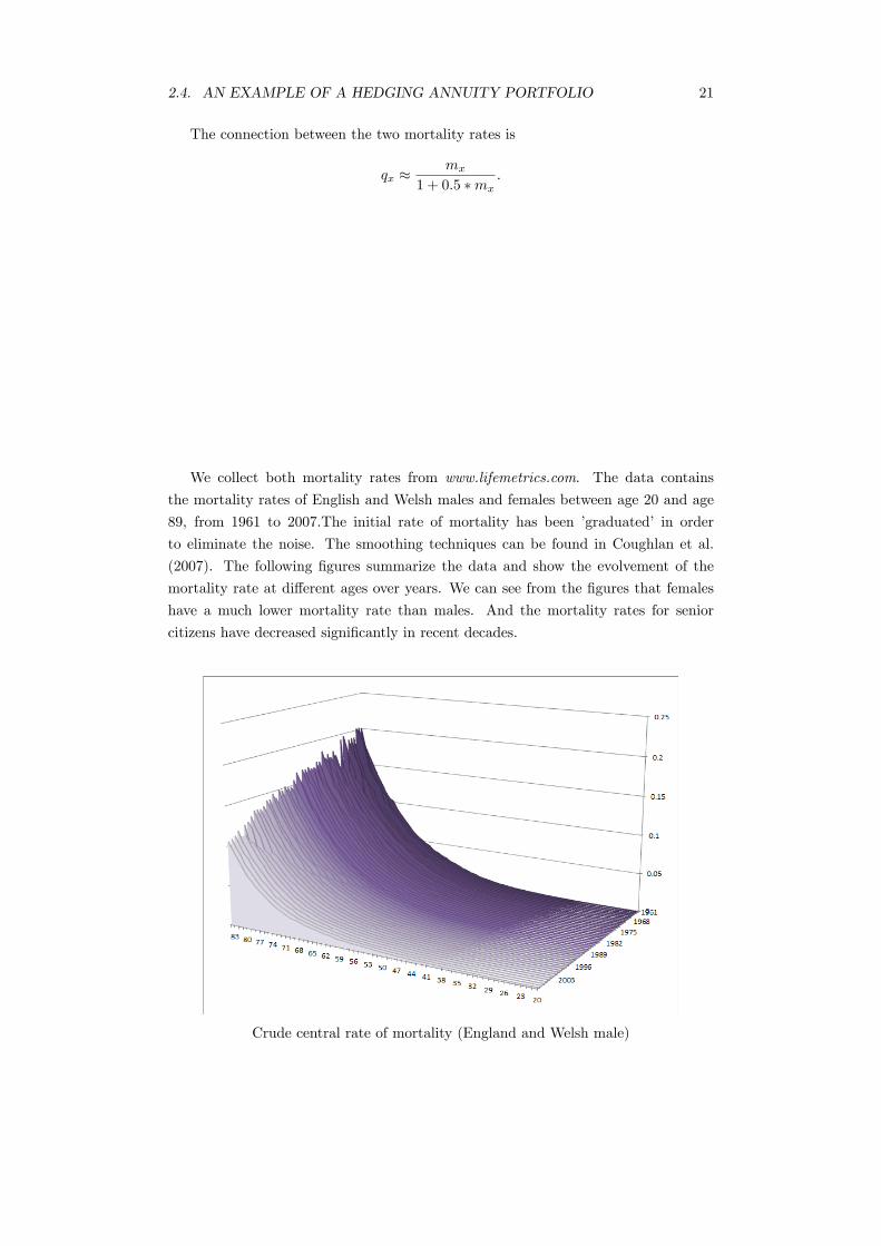
We collect both mortality rates from www.lifemetrics.com. The data contains
the mortality rates of English and Welsh males and females between age 20 and age
89, from 1961 to 2007.The initial rate of mortality has been ’graduated’ in order
to eliminate the noise. The smoothing techniques can be found in Coughlan et al.
(2007). The following figures summarize the data and show the evolvement of the
mortality rate at different ages over years. We can see from the figures that females
have a much lower mortality rate than males. And the mortality rates for senior
citizens have decreased significantly in recent decades.
Crude central rate of mortality (England and Welsh male)

22 CHAPTER 2. GENERALIZED QUADRATIC HEDGING STRATEGIES
Crude central rate of mortality (England and Welsh female)
Graduate initial rate of mortality (England and Welsh, male)

2.4. AN EXAMPLE OF A HEDGING ANNUITY PORTFOLIO 23
Graduate initial rate of mortality (England and Welsh, female)
Mortality intensity
Inspired by Dahl, Melchior and Møller (2008) [5], we assume the initial mortality
intensity to take the Gompertz-Makeham form. That is to say, the force of mortality
can be expressed as
µo(x+ t) = a+ b cx+t,
where a, b and c are positive constants. We focus on this age group between 30
and 80-year old. The next task is to fit the Gompertz-Makeham mortality curve to
the data. At this stage, we assume the mortality rate remains constant within a year,
which means that the central mortality rate equals the mortality intensity (See Cairns
et al. (2007) [2] for details). Therefore, the data considered here are the observed
central mortality rates of all the ages at one year. Here we adopt a least square
estimation method. Denote the observations as yi, where i represents the age. The
parameters of the model, a, b, c, are estimated by minimizing the objective function
∑i
(yi −
(a+ b (c)
i))2
, i = 29.5, 30.5, ..., 79.5.
Here 0.5 has been subtracted from the age since crude mortality date have been
used. The following figures show the fitted Gompertz-Makeham mortality curves for
English and Welsh females between years 1961 and 2007.

24 CHAPTER 2. GENERALIZED QUADRATIC HEDGING STRATEGIES
However, a deterministic mortality intensity curve is not enough. Following the
idea proposed by Dahl, Melchior and Møller (2008), we multiply the initial determin-
istic mortality curve by a CIR process to capture the stochastic evolvement of the
mortality curve over time. Consider the following CIR noise
dξt = (δ exp (−γt)− δξt) dt+ σ√ξtdW (t).
It can be easily shown that the mortality intensity µ(x, t) = µo(x+ t)ξ(t) is again
a CIR process.
The trick here is to leverage the probability to survive from time t to T , which
resembles the zero-coupon bond price in terms of its mathematical form
P (Tj,i > T | Ft) = E[e−
∫ Ttµj(x,s)ds
∣∣∣ Ft] = expA (T − t)−B (T − t)µj(x, t)
.
where A (T − t) and B (T − t) are deterministic functions, containing the parame-ters γ, δ, σ (See Dahl, Melchior and Møller (2008) for the forms of these two functions).
Please notice that the central rate of mortality is an analogue of the yield to maturity
of a one-year zero-coupon bond.
The parameters are estimated by minimizing the difference between the observed
central mortality rate y and the theoretical central mortality rate −A (T − t) +
B (T − t) (T − t)
minγ,δ,σ
∑(y +A (T − t; γ, δ, σ)−B (T − t; γ, δ, σ)µj(x, t)
)2.

2.4. AN EXAMPLE OF A HEDGING ANNUITY PORTFOLIO 25
Remark 10 The mortality intensity and the survival probabiliy obtained in this wayare the ones under the physical meausre P . For pricing purposes, one should either
change the measure to Q or estimate directly under the risk-neutral measure Q. The
latter method would involve market price data of some life-insurance contracts or
derivatives.
The following graph shows the stochastic intensity process over 20 years for Eng-
land and Welsh females aged 60 at time 0. The estimated parameters are
a b c γ δ σ
0.000729 0.000014 1.112223 0.3316 0.0138 0.0552
Stochastic mortality intensity (50 paths, 100 steps per year)
For a pool of 100 60-year old females (l = 100), the number of people surviving
over the next 20 years based on the proposed mortality intensity are shown by the
following figure.

26 CHAPTER 2. GENERALIZED QUADRATIC HEDGING STRATEGIES
Survivors counting process (50 paths, 100 steps per year)
Annuity portfolio and hedging
In this section, we show the simulated value of the annuity portfolio and mortality
forwards and some examples of hedging. For pricing and hedging purposes, we adopt
the following parameters for the mortality intensity process of the annuity portfolio
a1 b1 c1 γ1 δ1 σ1
−0.0013 0.0001 1.0956 0.3316 0.0138 0.0552
and the following parameters for the mortality forward
a2 b2 c2 γ2 δ2 σ2
−0.0013 0.0001 1.0956 0.1230 0.0207 0.0354
Further assume that the correlation coeffi cient is ρ = 0.85. The constant payment
to the survivors remains 1. The following figures show the simulated paths of the
values of annuity portfolios and the mortality forwards.

2.4. AN EXAMPLE OF A HEDGING ANNUITY PORTFOLIO 27
Annuity portfolio (100 paths, 100 steps per year)
Mortality forward (100 paths, 100 steps per year)

28 CHAPTER 2. GENERALIZED QUADRATIC HEDGING STRATEGIES
Right now let us look at a hedging example. Assume λ = 0.5. The following
graphs give the units of the risky assets and riskless assets which should be used
for the hedging portfolio. All the three quadratic hedging strategies, self-financing,
risk-minimization and generalized hedging, follow the same strategy for risky asset.
Number of risky asset
However, the strategy for riskless asset are different. In the following figures, the
blue indicates the units of riskless asset used in self-financing strategy, the black one is
for risk-minimization strategy and the red one is for the generalized quadratic strategy

2.5. CONCLUSION 29
with λ = 0.5.
Number of riskless assets
2.5 Conclusion
In this study, we design a new set of quadratic hedging strategies, which can balance
the short-term risk (additional cost risk) and the long-term risk (hedging error). The
unique optimal hedging strategy under the risk-neutral measure can be obtained via
a Kunita-Watanabe decomposition when λ = (0, 1). Though the model is more
complicated, the optimal trading strategy for the risky asset is the same with the
ones in the risk-minimization strategy and the self-financing strategy, however the
trading strategy for the riskless asset is very different.
In the empirical and numerical analysis part, we adopt mortality forwards to hedge
the longevity risk in an annuity portfolio. We apply the generalized quadratic hedging
strategy with λ = 0.5 and compare with the two traditional hedging strategies.

30 CHAPTER 2. GENERALIZED QUADRATIC HEDGING STRATEGIES

Bibliography
[1] P. Barrieu, L. Albertini (2009). The Handbook of Insurance-Linked Securities.
Wiley, Chichester.
[2] Cairns, A.J.G., Blake, D., Dowd, K. (2008) Modelling and management of mor-
tality risk: a review. Scandinavian Actuarial Journal 2008(2-3): 79-113.
[3] G. Coughlan, D. Epstein, A. Ong, A. Sinha, J. Hevia-Portocarrero, E. Gingrich, M.
Khalaf-Allah, P. Joseph (2007). LifeMetrics: A toolkit for measuring and managing
longevity and mortality risks. www.lifemetrics.com
[4] M. Dahl, T. Møller (2007). Valuation and Hedging of Life Insurance Liabilities
with Systematic Mortality Risk, Insurance. Mathematics and Economics 39, 193-
217.
[5] M. Dahl, M. Melchior and T. Moller (2008). On systematic mortality risk and
risk-minimization with survivor swaps. Scandinavian Actuarial Journal. Vol 2008,
Issue 2-3.
[6] M. Ehrgott (2005). Multicriteria optimization. Birkhäuser.
[7] H. Föllmer, D. Sondermann (1986). Hedging of Non-redundant Contingent Claims.
Contributions to Mathematical Economics. North-Holland, 205-223.
[8] T. Møller (2001). Risk-minimizing Hedging Strategies for Insurance Payment Pro-
cesses. Finance and Stochastics. Vol 5, No. 4. 419-446.
[9] M. Schweizer (2001). A Guided Tour through Quadratic Hedging Approaches.
Option Pricing, Interest Rates and Risk Management. Cambridge University Press
(2001), 538—574.
[10] M. Schweizer (2008). Local Risk-Minimization for Multidimensional Assets and
Payment Streams. Banach Center Publications 83, 213-229.
31

32 BIBLIOGRAPHY
Chapter 3
Risk-Neutral Densities andMetal Futures
3.1 Introduction
Harrison and Kreps (1979) [10] and Harrison and Pliska (1981) [11] established the
link between no-arbitrage pricing and martingale theory. The first fundamental asset
pricing theorem states that the absence of arbitrage in the market is equivalent to
existence of an equivalent martingale measure Q for the price process of the under-
lying financial asset. The second fundamental asset pricing theorem states that the
completeness of a market is equivalent to uniqueness of the equivalent martingale
measure. (see Kiesel (2002) [14] for more details.) In reality, the markets are seldom
complete due to undiversifiable and unhedgeable risks. As a result, there could exists
multiple pricing measures that can rule out arbitrage opportunities. This comparative
study considers three pricing measures obtained by different approaches and applies
them to different commodity future markets.
It is important to identify the difference between forward and future prices when
the interest rate is stochastic. At time t, denote the prices of forward and future
contracts expiring at time T to be ForS(t, T ) and FutS(t, T ),respectively. Let S(t)
be the spot price at time t and B(t, T ) be the price of a zero-coupon bond paying 1
at time T .
Definition 11 (Shreve(2000) [19]) Assume that zero-coupon bonds of all maturitiescan be traded. Then the forward price is determined by
ForS(t, T ) =S(t)
B(t, T ), 0 ≤ t ≤ T,
Definition 12 (Shreve(2000) [19]) The futures price of an asset is given by the for-mula
FutS(t, T ) = EQ [S(T ) | Ft] .
33
34 CHAPTER 3. RISK-NEUTRAL DENSITIES AND METAL FUTURES
A long position in the futures contract is an agreement to receive as a cash flow
the changes in the futures price (which may be negative as well as positive) during the
time the position is held. A short position in the futures contract received the opposite
cash flow.
The difference between forward and future prices is the so-called forward-futures
spread.
Commodity futures have been intensively studied in the literature. Schwartz
(1997) [18] compared three models and found out that the dynamics of futures prices
can be captured by three factors: driving spot prices, interest rates and convenience
yields. The convenience yield, according to Carmona and Ludkovshi (2005) [4], is de-
fined as the difference between benefit of direct access and cost of storage. Later on,
a lot of new models for commodity spot prices and future prices have been proposed
and empirically studied. (Ross (1997) [17], Casassus and Collin-Dufresne (2002) [5],
Carmona and Ludkovski (2005), etc)
The focus of this study is not on the dynamics of commodity spot or future prices,
but on the link between spot and future prices. The essay considers three measure-
changing approaches. We aim to find out the best measure-changing technique in
terms of empirical performance. We also would very much like to quantify the perfor-
mance of the frequently studied measure-changing techniques like Esscher transform
compared to calibration method and the non-parametric method. This is important
because techniques like Esscher transform do not require the availability of derivatives
prices and thus have often been adopted to study illiquid, not yet mature markets,
like the insurance derivatives market discussed in the previous chapter.
The article is structured as follows. The first section describes the three measure-
changing techniques. The second section empirically analyzes the performance of the
methods on three commodity markets, gold, copper, and aluminum. The last section
concludes the results.
3.2 Method1: price commodity futures under the
Esscher measure
3.2.1 Dynamics for the commodity spot prices
We work on a probability space (Ω,F , P ). In this section, we will adopt the following
SDE to describe the dynamics of the commodity spot prices.
St = S0 exp(Gt),
where
dGt =(µG − λGGt−
)dt+ σt dLt,
dσ2t = (κ− ησ2
t−)dt+ φσ2t− d[L,L]dt .

3.2. METHOD1: PRICE COMMODITY FUTURES UNDER THE ESSCHERMEASURE35
The process G follows a COGARCH process, as proposed by Klüppelberg, Lindner
and Maller (2004) [15]. We denote the augmented filtration generated by G and σ2
with F.L is a Lévy process with differential triplet (b, c, F (dx)) .For simplicity, we assume
the L process to be a NIG process. As we will see later, this process provides a good
fit to the commodity data. With parameters α, β, µ, δ, a NIG random variable has
the density function. Here K1(.) is the modified Bessel function of the third kind with
index 1.
gNIG(α,β,µ,δ)(z) =α exp(ς + β(z − µ))K1(αδq((z − µ)/δ))
πq((z − µ)/δ),
ς = δ
√α2 − β2, q(x) =
√1 + x2,
0 < |β| < α, −∞ < µ <∞, δ > 0.
For a COGARCH model, we always require that L has mean zero and unit vari-
ance. To this purpose, we reparameterize NIG(α, β, µ, δ) to NIG(ξ, ρ, κ1, κ2), where
κ1 represents the mean value and κ2 represents the variance.
ξ = (1 + ς)−1/2, ρ = β/α,
κ1 = µ+ δρ/√
1− ρ2 = 0, κ2 = δ2/(ς(1− ρ2)
)= 1.
The NIG process is a pure jump process. Therefore its differential triplet reduces
to (b, 0, F (dx)), where the drift term b and Lévy measure F (dx) are given by
b = µ+2δα
π
∫ 1
0
sinh (βx)K1 (αx) dx
F (dx) =δα
π |x|eβxK1 (α |x|) dx
Proposition 13 Assume(σ2t
)t≥0
is the stationary version of the process with σ20 =
σ2∞. If the underlying asset price S follows a COGARCH model then the future price
reduces to
FutS(t, T ) = S(t)ϕQG (t, T ; 1)
where ϕQG is the Laplace transform of G with parameter 1 and Q is a risk-neutral
measure.
Proof. We have
FutS(t, T ) = EQ [S(T ) | Ft]
= EQ [S0 exp(GT −Gt +Gt) | Ft]
= S(t)EQ [ exp(GT −Gt) | Ft]
= S(t)EQ [exp(GT−t)]
= S(t)ϕQG (t, T ; 1) .

36 CHAPTER 3. RISK-NEUTRAL DENSITIES AND METAL FUTURES
Here the fourth equal sign holds because of the stationary increment property of G.
3.2.2 Risk-neutral distribution estimated from spot price data
For two probability measures Q and P defined on a measurable space (Ω,F), Q is
said to be absolutely continuous with respect to P if all P -zero sets are also Q-zero
sets, denote as Q P . P and Q are considered to be equivalent if Q P and
P Q. If Q P , there exists a unique density Z = dQ/dP so that for f ∈ L1 (Q)
the following equation holds
EQ [f ] = EP [Zf ] .
One can associate a martingale with respect to Z,
Zt = EP [Z| Ft] .
This martingale is the density process of Q.
For the following definitions and notation we refer to Jacod and Shiryaev(2003)
[12]. Assume that X is a semimartingale and there exists θ ∈ L (X) such that θ ·X is
exponentially special, where · denotes stochastic integration. The Laplace cumulantKX(θ) is defined as the compensator of the special semimartingale Log
(eθ·X
). We
have
KX(θ) = κ(θ) ·A,
where
κ(θ)t = θtbt +1
2θ2t ct +
∫ (eθtx − 1− θth (x)
)Ft (dx) .
Here b, c, F are the differential characteristics of X. h : R −→ R is a truncation
function, which are bounded and satisfy h(x) = x in a neighbourhood of 0.
The modified Laplace cumulant KX (θ) is defined as
KX(θ) = log E(KX(θ)
),
If X is quasi-left continuous then KX(θ) = KX(θ) and KX(θ) is continuous.
A càdlàg process X is defined as quasi-left continuous if ∆XT = 0 a.s. on the set
T <∞ for every predictable time T . In our case, G is quasi-left continuous becauseL is a NIG process.
In an incomplete market, which is the case when we adopt Lévy-driven asset
process, we could face plenty of different risk-neutral measures with different density
process. In this study, we focus on the widely used Esscher measure [12] with thedensity process
Zt = exp
(∫ t
0
θs dXs −KX(0, t; θ.)
).

3.2. METHOD1: PRICE COMMODITY FUTURES UNDER THE ESSCHERMEASURE37
3.2.3 Futures price under the Esscher measure
Our next goal is to find the process θ making the discounted spot price a martingale
under the Esscher measure Q. Because we are dealing with commodities, we have to
define the discounted spot price in a different way.
Commodities, unlike stocks or bonds, can be consumed or stored with some costs.
The difference between the consumption value and storage expenses per unit of time
is termed the convenience yield δ. Intuitively, the convenience yield corresponds to a
dividend yield for stocks (Carmona and Ludkovski (1991)). Therefore, the discount
rate should become to
rt − δt ,
and the discounted spot price changes to
St = exp
(−∫ t
0
(rs − δt) ds
)St .
It remains to specify a dynamic for δt. In this study, we adopt a convenience yield
proportional to G, i.e.
δt = λGGt−
for some constant λG. With these specifications, the Esscher measure, and there-
fore the risk-neutral spot price, can be determined.
Theorem 14 The discounted spot price is a Q-(local) martingale where θt satisfies
θt σ2t−c
2−rt+µG+σt−b+1
2σ2t−c
2 +
∫ (e(θt+1)σs−y − eθtσs−y − σt−h(y)
)F (dy) = 0.
Here (b, c2, F ) is the Lévy triplet of L.
Proof. The result can be proved by two different methods.
The first approach rests on Girsanov’s theorem. The density process admits the
representation
dZt = Zt θtσtcdWt + Zt
∫ (eθtσsx − 1
)(µ− ν)(ds, dt).
On the other hand, the discounted spot price process under P admits a stochastic
representation as
d(e−
∫ t0
(ru−λGGt−) duSt
)= St σtc dWt + St
∫(eσtx − 1) (µ− ν)(ds, dt)
+St
(−rt + λGGt− + σtb+
1
2σ2t c
2 +
∫(eσtx − 1− σth(x))F (dx)
)dt.
Therefore the predictable finite variation part in the decomposition of the discounted

38 CHAPTER 3. RISK-NEUTRAL DENSITIES AND METAL FUTURES
spot price process as a special semimartingale is
dAt = St
(−rt + λGGt− + σtb+
1
2σ2t c
2 +
∫(eσtx − 1− σth(x))F (dx)
)dt.
Whereas the predictable finite variation part of the discounted spot price process
under Q takes the form
dA+1
Z−d⟨Z, S
⟩= St
(θtσ
2t c
2 +
∫ (e(θt+1)σsx − eσtx − eθt σsx + 1
)F (dx)
−rt + λGGt− + σtb+1
2σ2t c
2
).
This part must be sent to zero in order to guarantee that the discounted spot price
process is a martingale under Q. In this way we end up with a Feynman—Kac type
equation
θtσ2t c
2 − rt + λGGt− + σtb+1
2σ2t c
2 +
∫ (e(θt+1)σsx − eθtσsx − σth(x)
)F (dx) = 0,
which proves the result.
In the alternative method, we first determine the differential characteristics of
G := −rt + λGGt− + Gt. Recall that in our case, the discounted spot price can be
written as
St = S0 exp(Gt
).
Let us define a new process
G(h) = G− G′(h),
where
G′(h)t =∑s≤t
[∆Gs − h(∆Gs)
].
G(h)t admits the representation
dG(h)t = dGt −∫
(σt−y − h(σt−y)) µ(dy, dt)
= −rtdt+ λGGt−dt+ dGt −∫
(σt−y − h(σt−y)) µ(dy, dt).
Therefore the differential characteristics of G are
bGt = −rt + λGGt− + µG − λGGt− + σt−b+
∫(h(σt−y)− σt−h(y))µ(dy, dt)
cGt = σt−c
F G(A)t =
∫1A(σt−y)F (dy).
3.2. METHOD1: PRICE COMMODITY FUTURES UNDER THE ESSCHERMEASURE39
According to Jacod and Shiryaev (2003) (page 224, theorem 7.18), the process eG is
a Q-local martingale if and only if θ · G is exponentially special and if we have
KG (θ + 1) = KG (θ) .
Therefore, by the definition of the Laplace cumulant and modified Laplace cumulant,
the equation in the theorem holds.
The above equation for θ can be explicitly solved when the driving Lévy process
is a NIG process.
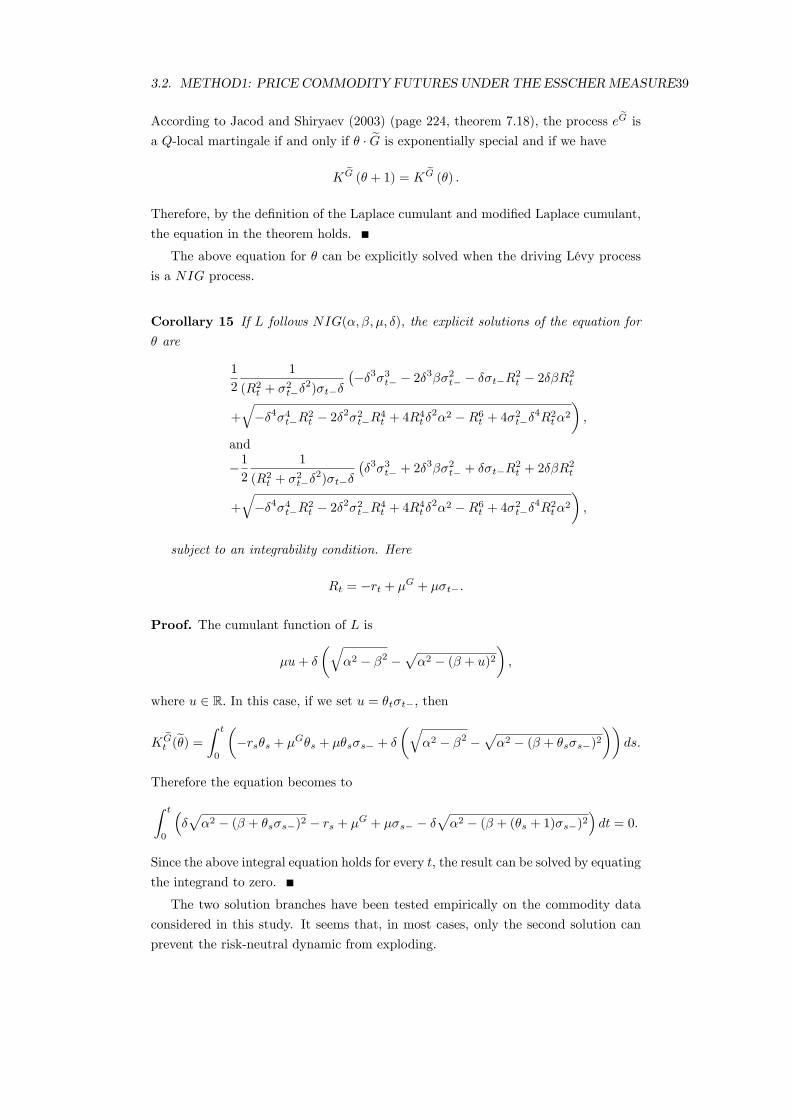
Corollary 15 If L follows NIG(α, β, µ, δ), the explicit solutions of the equation for
θ are
1
2
1
(R2t + σ2
t−δ2)σt−δ
(−δ3σ3
t− − 2δ3βσ2t− − δσt−R2
t − 2δβR2t
+√−δ4σ4
t−R2t − 2δ2σ2
t−R4t + 4R4
t δ2α2 −R6
t + 4σ2t−δ
4R2tα
2
),
and
−1
2
1
(R2t + σ2
t−δ2)σt−δ
(δ3σ3
t− + 2δ3βσ2t− + δσt−R
2t + 2δβR2
t
+√−δ4σ4
t−R2t − 2δ2σ2
t−R4t + 4R4
t δ2α2 −R6
t + 4σ2t−δ
4R2tα
2
),
subject to an integrability condition. Here
Rt = −rt + µG + µσt−.
Proof. The cumulant function of L is
µu+ δ
(√α2 − β2 −
√α2 − (β + u)2
),
where u ∈ R. In this case, if we set u = θtσt−, then
KGt (θ) =
∫ t
0
(−rsθs + µGθs + µθsσs− + δ
(√α2 − β2 −
√α2 − (β + θsσs−)2
))ds.
Therefore the equation becomes to∫ t
0
(δ√α2 − (β + θsσs−)2 − rs + µG + µσs− − δ
√α2 − (β + (θs + 1)σs−)2
)dt = 0.
Since the above integral equation holds for every t, the result can be solved by equating
the integrand to zero.
The two solution branches have been tested empirically on the commodity data
considered in this study. It seems that, in most cases, only the second solution can
prevent the risk-neutral dynamic from exploding.
40 CHAPTER 3. RISK-NEUTRAL DENSITIES AND METAL FUTURES
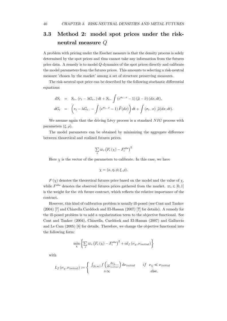
3.3 Method 2: model spot prices under the risk-
neutral measure Q
A problem with pricing under the Esscher measure is that the density process is solely
determined by the spot prices and thus cannot take any information from the futures
price data. A remedy is to model Q-dynamics of the spot prices directly and calibrate
the model parameters from the futures prices. This amounts to selecting a risk-neutral
measure ’chosen by the market’among a set of structure preserving measures.
The risk-neutral spot price can be described by the following stochastic differential
equations:
dSt = St− (rt − λGt−) dt+ St−
∫(eσt−x − 1) (µ− ν) (dx, dt),
dGt =
(rt − λGt− −
∫(eσt−x − 1) F (dx)
)dt+
∫(σt−x) µ(dx, dt).
We assume again that the driving Lévy process is a standard NIG process with
parameters (ξ, ρ).
The model parameters can be obtained by minimizing the aggregate difference
between theoretical and realized futures prices.
∑i
$i
(Fi (χ)− F obsi
)2Here χ is the vector of the parameters to calibrate. In this case, we have
χ = (κ, η, φ; ξ, ρ).
F (χ) denotes the theoretical futures price based on the model and the value of χ,
while F obs denotes the observed futures prices gathered from the market. $i ∈ [0, 1]
is the weight for the ith future contract, which reflects the relative importance of the
contract.
However, this kind of calibration problem is usually ill-posed (see Cont and Tankov
(2004) [7] and Chiarella Carddock and El-Hassan (2007) [?] for details). A remedy forthe ill-posed problem is to add a regularization term to the objective functional. See
Cont and Tankov (2004), Chiarella, Carddock and El-Hassan (2007) and Galluccio
and Le Cam (2005) [8] for details. Therefore, we change the objective functional into
the following form:
minχ
∑i
$i
(Fi (χ)− F obsi
)2+ αlf (νχ, νinitial)
with
Lf (νχ, νinitial) :=
∫(0,∞)
f(
dνχdνinitial
)dνinitial if νχ νinitial
+∞ else.

3.4. METHOD 3: NON-PARAMETRIC ESTIMATIONOF RISK-NEUTRAL DENSITIES41
The function f is chosen to be
f(x) = x log(x)− x+ 1.
The existence of a solution for this regularization calibration problem has been
proved by Keller-Ressel (2006) [13].
3.4 Method 3: non-parametric estimation of risk-
neutral densities
Grith, Härdle and Schienle (2010) [9] proposed a non-parametric approach to estimate
risk-neutral density from option prices. In this study, their idea will be applied to
futures markets.
There is a link between the p, the conditional density function of the physical
measure, and q, the conditional density function of the risk-neutral measure, namely
q (ST | Ft) = m (ST | Ft) p (ST | Ft) .
Here m is the pricing kernel, which summarizes information related to asset pric-
ing. We cannot incorporate all the factors driving the form of the pricing kernel, so
we consider the projection of the pricing kernel on the set of available payoff functions
and denote it as m∗. Assume it is close to m in the sense that
‖m−m∗‖2 =
∫|m(x)−m∗(x)|2 dx < ε.
Further assume m∗ has a Fourier series expansion
m∗ (ST | Ft) =∞∑l=1
αl,tgl (ST | Ft)
where αl are Fourier coeffi cients and gl is a fixed collection of basis functions.Following
Grith, Härdle and Schienle (2010), we adopt the Laguerre polynomials to conduct em-
pirical analysis. In practice, we can only expand m∗ up to a finite number L, which
gives us an approximation
m (ST | Ft) =L∑l=1
αl,tgl (ST | Ft) .
The remaining task is to estimate αl,t from the derivative prices data. The com-
modity future prices can be expressed in the following way:
Yi,t = e−rt∫ ∞
0
STL∑l=1
αl,tgl (ST | Ft) p (ST | Ft) dST + εi
=L∑l=1
αl,t
e−rt
∫ ∞0
ST gl (ST | Ft) p (ST | Ft) dST
+ εi.

42 CHAPTER 3. RISK-NEUTRAL DENSITIES AND METAL FUTURES
Set
ψil = e−rt∫ ∞
0
ST gl (ST | Ft) p (ST | Ft) dST .
Finally we can obtain a feasible estimator of α by least-square estimation
α =(
ΨT Ψ)−1
ΨTY
which will give us the pricing kernel
m (ST | Ft) = g (ST | Ft)ᵀ α
and hence the risk-neutral density.
3.5 Empirical analysis
3.5.1 Estimation method and simulation techniques
Estimate P -dynamic parameters
The COGARCH model can be estimated by a pseudo-maximum likelihood (PML)
method proposed by Maller, Müller and Szimayer (2008) [16]. Suppose we have
observations G(ti), 0 = t0 < t1 < ... < tN = T. In Maller, Müller and Szimayer
(2008)’s case, Yi is defined as the difference between G(ti) and G(ti−1), i.e., the
observed returns.
In our case, we define Yi in a different way in order to facilitate the estimation
procedure, namely
Yi := G(ti)−G(ti−1)−(µG − λGG(ti−1)
)∆ti =
∫ ti
ti−1
σ(s−)dL(s).
Assuming the Yi are conditionally normal, we can write a pseudo-log-likelihood
function for Y1, ..., YN as
LN ($, η, φ) = −1
2
N∑i=1
Y 2i
ρ2i
− 1
2
N∑i=1
log(ρ2i )−
N
2log(2π)
where
ρ2i : = E
[Y 2i
∣∣ Fti−1] ≈ σ2(ti−1)∆ti
σ2(ti) = $∆ti−1 + φe−η∆ti−1Y 2i−1 + e−η∆ti−1σ2(ti−1).
This method can handle both regularly spaced data and irregularly spaced data.

3.5. EMPIRICAL ANALYSIS 43
Simulate Q-dynamics
Another problem with the Esscher measure is that it sometimes changes the model
class of the driving process, which happens in this case. After measure-changing the
driving process L is not a NIG process anymore due to the time-varying σ and θ.
This increases the diffi culty to simulate GQ, the G process under Q. One way to do
it is to approximate dGQ by the following process:
dGQt = rtdt+ σtdWt +d∑i=1
ci,t∆N(i)t − ci,tλi,t1|ci,t|≤1dt
The logic here is to approximate large jumps by d nonhomogeneous Poisson pro-
cesses N (i)t , 1 ≤ i ≤ d, and small jumps by a Brownian motion with volatility
σ2t =
∫|x|<ε
x2F ∗t (dx)
where
F ∗t (dx) = eθtσt−xF (dx).
Approximating small jumps by a Brownian motion is a commonly used technique
and can achieve more accurate results than certain alternative approaches (Asmussena
and Glynn (2007) [1]). However, this approximation is not always feasible. A rigorous
discussion for Lévy case was provided by Asmussen and Rosinski (2001) [2], suggesting
the necessary condition for the approximation,
ε/σε → 0,
holds if and only if
σcσε∧ε ∼ σε.
For a NIG process, Asmussen and Rosinski (2001) prove that the approximation
is valid. In our case, after the measure-changing, F ∗t (dx) resembles the Lévy measure
of a NIG process with time-varying parameter β∗ = β − θtσt,
F ∗t (dx) = ν(dx) =δα
π |x|e(β−θtσt)xK1 (α |x|) dx.
Next, let us look at the approximation of the big jumps. We adopt a nonhomoge-
neous Poisson process with intensity process
λi,t =
F ∗t ([ai−1, ai)) 1 ≤ i ≤ kF ∗t ([ai, ai+1)) k + 1 ≤ i ≤ d
and time-changing jump sizes
c2i,tλi,t =
∫ ai−ai−1
x2F ∗t (dx) 1 ≤ i ≤ k∫ ai+1−ai
x2F ∗t (dx) k + 1 ≤ i ≤ d.

44 CHAPTER 3. RISK-NEUTRAL DENSITIES AND METAL FUTURES
Here, ai are real-numbers satisfying
a1 < ... < ak = −ε
ε = ak+1 < ... < ad
ε ∈ (0, 1).
We choose ε = 0.3, a1 = −5.3, ad = 5.3. All the integrals are approximated by the
composite Simpson’s rule and the nonhomogeneous Poisson processes are generated
by the algorithm in [3].
Numerical approximation of integrals
This study involves quite a lot of integrals such that explicit solutions are very diffi cult
to obtain. In this case, a numerical approximation has been used. An integral between
two finite numbers can be approximated by the composite Simpson’s rule
∫ b
a
f(x)dx ≈ h
3
[f (x0) + 2
n/2−1∑j=1
f (x2j) + 4n/2∑j=1
f (x2j−1) + f (xn)
].
For integrals without finite boundary, a transformation must be adopted first, e.g.∫ ∞0
f(x)dx =
∫ 1
0
f
(t
1− t
)1
(1− t)2 dt.
3.5.2 Gold and gold future market
Gold has played an important role in the development of civilization. It was firstly
used for decoration and then served as a store of wealth and a medium of trade.
Nowadays people possess gold to hedge the risks generated from economic or political
events. Figure 1 show the gold spot prices and the logarithm of gold spot prices
between 26/11/2008 and 26/10/2010. The data is of daily scope and all the non-
trading days have been excluded.
Gold futures provide hedging tools for commercial producers and users of gold, op-
portunities for portfolio diversification and global gold price discovery (http://www.cmegroup.com).
I considered the 11 gold futures traded on COMEX (New York Commodity Exchange,
Inc.) for empirical study: GCG09, GCJ09, GCM09, GCQ09, GCV09, GCZ9, GCG0,
GCJ0, GCM0, GCQ0, GCV0. Here GC is the product symbol. The third letter and
the followed numbers state the expiry month and year of the contract. Trades of the
contract are allowed until three working days before the settlement month. Figure 2
shows the gold future prices surface. We are considering the settlement prices of 11
gold future contracts between 26/11/2008 and 26/10/2010.

3.5. EMPIRICAL ANALYSIS 45
All the data are downloaded from the bloomberg terminal.
Gold spot price
Fit the model under the P measure
The first task is to fit the model to the gold spot price. If we assume the data points
are regularly spaced, i.e., ignore the non-trading days, the estimates of parameters
areκ η φ µG λ
2.1662e− 06 0.0558 0.0380 0.0016 0.0023
The estimates were obtained by PMLE. So we need to have a closer look of the
standardized residuals in the return function. First of all, we did a Jarque-Bera test
to test the normal assumption of the PMLE. It can be seen from the result that the
normal distribution assumption can be rejected.
Jarque−Bera p− value34.6801 0.00000
Secondly, we try to fit a standardized NIG distribution. The following table and
figure give the maximum likelihood estimates to the four parameters of the NIG
distribution and the comparison between the histogram of the standardized residual
and the density function of the NIG distribution with the four estimated parameters.
α β µ δ
1.7182171 −0.3124525 0.3021202 1.6336979

46 CHAPTER 3. RISK-NEUTRAL DENSITIES AND METAL FUTURES
Finally, we check the fitted NIG distribution by the Chi-square test. Unfortu-
nately, the test result suggests the standard residuals do not follow the fitted NIG
distribution.
Chi2stat p− value39.6754 0.0000
Right now let us look at the case when the non-trading days are considered. Put
it in another way, the data points are irregularly spaced. Let us do the PMLE again
to fit the model parameters and check the distribution assumption of the standard
residuals.
κ η φ µG λ
1.0526e− 06 0.0333 0.0275 −9.3388e− 05 −0.0014
Jarque−Bera p− value39.048 0.00000
Again, the normality assumption is rejected. So I tried the standard NIG distri-
bution again. The following results are the estimated values of the parameters and
the histogram.
α β µ δ
1.6959514 −0.3029201 0.2932561 1.6154437

3.5. EMPIRICAL ANALYSIS 47
This time the standard NIG assumption cannot be rejected by the goodness-of-fit
test. Therefore, in the following part, we will only focus on the model estimated under
the irregular spaced data assumption.
Chi2stat p− value7.35 0.3934
The realized θ process
The next task is to find out the realized θ, which determines the realized Esscher
measure. We can see from the picture that θ, the sole factor to determine the risk
premium, is indeed a stochastic process in the gold future market. The positive value

48 CHAPTER 3. RISK-NEUTRAL DENSITIES AND METAL FUTURES
of θ means that jump sizes tend to be bigger under the pricing measure Q.
The realized theta (26/11/2008-26/10/2010)
Theoretical future prices
The last task is to find out the theoretical future prices determined by the three
approaches and compare them with the realized gold future prices.

3.5. EMPIRICAL ANALYSIS 49
The above show the result of the first method. The first figure shows the fitness
of the theoretical future prices to the real future curve on 28 Nov 2008. The second
figure tells the percentage difference of the model prices and real prices during the
following 30 trading days. The average of the absolute values of percentage difference
in this period is 2.706%.

50 CHAPTER 3. RISK-NEUTRAL DENSITIES AND METAL FUTURES
The above is the result of the second method. The model is fitted by the historical
future curves on 5 trading days until (including) 28 Nov 2008. The first figures shows
the performance of the model on 28 Nov 2008. The second shows the performance of
the same model for the following 30 trading days. The average of the absolute values
of percentage difference is 0.8509%. The calibrated parameters during this period are
κ η φ λ α β µ δ
6.34E − 07 0.559 0.0275 0.0024 1.3863 −1.2147 0.282 0.1551

3.5. EMPIRICAL ANALYSIS 51
The above is the result of the third method. The model is fitted by the historical
future curves on 5 trading days until (including) 28 Nov 2008. The first figures shows
the performance of the model on 28 Nov 2008. The second shows the performance of
the same model for the following 30 trading days. The average of the absolute values
of percentage difference is 0.2876%. Obviously, the third method achieves the best fit
to the real market prices.

52 CHAPTER 3. RISK-NEUTRAL DENSITIES AND METAL FUTURES
3.5.3 Copper and copper future market
Due to its vast quantity, copper has been for a long time an important material for
weapon and household objects in the history. In the modern era, copper has been
widely used in electrical and electronic products. The following figure shows the
copper spot prices between 26/11/2008 and 26/10/2010.
Copper futures are traded on several exchanges: LME (London Metal Exchange),
COMEX, SHME (Shanghai Metal Exchange) etc. This study considers 11 future
contracts traded on LME: LPG09, LPJ09, LPM09, LPQ09, LPV09, LPZ9, LPG0,
LPJ0, LPM0, LPQ0, LPV0.
Copper spot price
Fit the model under the P measure
We firstly fit the P model to the spot data. Under the regular space assumption, the
estimated value of the parameters are
κ η φ µG λ
7.1434e− 06 0.0951 0.0828 0.0051 0.0055
Normality assumption of the standardized residuals can be rejected.
Jarque−Bera p− value9.3126 0.0095
Again we choose standard NIG as a candidate distribution for the standardized

3.5. EMPIRICAL ANALYSIS 53
residuals and check this assumption by the goodness-of-fit test. The SNIG cannot
be rejected.
α β µ δ
3.2182479 −0.6807412 0.6502828 3.0046911
Chi2stat p− value4.3212 0.8270
And then we repeated the above procedure to fit the model under the irregular
spaced data assumption. The following are the estimated parameters. Jarque-Bera
test is again significant.
$ η φ µG λ
3.2007e− 06 0.0540 0.0568 0.0028 0.0023
Jarque−Bera p− value10.9453 0.0042
Therefore I tried the SNIG distribution and check the new assumption by the
goodness-of-fit test. The SNIG assumption cannot be rejected.

54 CHAPTER 3. RISK-NEUTRAL DENSITIES AND METAL FUTURES
α β µ δ
3.1315263 −0.6307958 0.6052008 2.9428774
Chi2stat p− value11.3803 0.0773
Although the model is valid under both regularly spaced data assumption and
irregularly spaced data assumption, we will only adopt the model under the irregularly
spaced data assumption to estimate the theoretical future price.
Realized θ process
The copper future market also witnesses a stochastic θ. However, unlike the gold
future market, the realized θ process in the copper future market always take negative
value, which means the jump size under Q tend to be smaller than the one under P .

3.5. EMPIRICAL ANALYSIS 55
The realized theta (26/11/2008-26/10/2010)
Theoretical future prices
Finally let us look at the comparison between the theoretical copper future prices and
the realized ones.

56 CHAPTER 3. RISK-NEUTRAL DENSITIES AND METAL FUTURES
The above are the results of the first method. In-the-sample experiment shows an
average absolute values of percentage difference of 4.8347%.

3.5. EMPIRICAL ANALYSIS 57
The above show the results of the second method. The average of the absolute
values of percentage difference is 1.3073%. The calibrated parameters during this
period are as follows
κ η φ λ α β µ δ
2.97E − 06 0.802 0.0339 0.0028 0.2528 −0.2385 0.0263 0.0093

58 CHAPTER 3. RISK-NEUTRAL DENSITIES AND METAL FUTURES
The above are the results of the third method. The average of the absolute values
of percentage difference is 0.291%. Again, the third method outperformed the other
two.
3.5.4 Aluminum and aluminum future market
Aluminium is an important industrial material and has wide application in construc-
tion and manufacturing. Aluminum also substitutes for copper in many areas.The
following figure show the aluminum spot price between 26/11/2008 and 26/10/2010.
We considered 11 aluminum future contracts traded on LME between 26/11/2008
and 26/10/2010.

3.5. EMPIRICAL ANALYSIS 59
Aluminium spot price
Fit the model under the P measure
The empirical analyzes starts again with fitting the P model to the spot price. The
following are the values of the estimated parameters under the regular space assump-
tion.κ η φ µG λ
1.3167e− 05 0.0706 0.0312 0.0011 0.0037
Normality assumption of the standardized residuals can be again rejected.
Jarque−Bera p− value51.4619 0.0000
A standard NIG distribution has been adopted to describe the distribution of the
standardized residuals. The following table show the estimates.
α β µ δ
2.2156312 −0.4329320 0.4164023 2.0899585
The shape histogram shows similarity to the shape of the density function of the
fitted SNIG distribution. The distribution assumption cannot be rejected by the
test.

60 CHAPTER 3. RISK-NEUTRAL DENSITIES AND METAL FUTURES
Chi2stat p− value3.4897 0.7453
Consider the model again under the irregular spaced data assumption. The fol-
lowing are the estimated parameters and the result of the Jarque-Bera test.
κ η φ µG λ
9.6356e− 06 0.0591 0.0302 6.4010e− 05 −0.0023
Jarque−Bera p− value129.4878 0.0000
Fit a SNIG distribution to the data and test it with the goodness-of-fit test. The
SNIG assumption cannot be rejected.
α β µ δ
1.19206241 −0.05224162 0.05214129 1.18862986

3.5. EMPIRICAL ANALYSIS 61
Chi2stat p− value3.3442 0.7646
Theoretical future prices
The followings compare the theoretical and observed future prices.

62 CHAPTER 3. RISK-NEUTRAL DENSITIES AND METAL FUTURES
The above are the results of the first method. For the in-the-sample performance,
the average of the absolute values of percentage difference is 8.0913% .

3.5. EMPIRICAL ANALYSIS 63
The above are the results of the second method. The average of the absolute
values of percentage difference is 4.4504%. The calibrated parameters are
κ η φ λ α β µ δ
9.45e− 06 0.0273 0.0862 −0.0862 0.6206 0.0564 −0.0560 0.6129

64 CHAPTER 3. RISK-NEUTRAL DENSITIES AND METAL FUTURES
The above are the results of the third method. The average of the absolute values
of percentage difference is 1.6252%.
Not surprisingly, the third method showed for the third time to be the best among
all the methods considered.
3.6. CONCLUSION 65
3.6 Conclusion
This research studied three measure-changing approaches and applied them to three
commodity future markets: gold, copper and aluminum. The empirical analysis shows
that the nonparametric measure-changing method give the best fit to the observed
future prices in all the three markets.
In my opinion, the main reason for the relative underperformance of the first ap-
proach is that a model fitted from time-series data is probably incapable of capturing
cross-section phenomenon. We may change this by modeling the whole futures curve
and the stochastic evolvement of the curve, just like what we did in the previous
chapter to model the mortality intensity.
The reason for the underperformance of the second model is the structure of the
spot price dynamics. It would be beneficial to model the convenience yield or the
volatility in a different way.
The main purpose of this essay is to quantify the relative performance of the three
methods in a market with many liquid futures present, in view that in some of the
new financial markets with only very few futures or derivatives available, one has to
resort to pricing by optimal martingale measures like the Esscher measure.

66 CHAPTER 3. RISK-NEUTRAL DENSITIES AND METAL FUTURES

Bibliography
[1] S. Asmussen, P.W. Glynn (2007). Stochastic simulation: algorithms and analysis.
Springer.
[2] S. Asmussen, J. Rosinski (2001). Approximations of small jumps of Lévy processes
with a view towards simulation. Journal of Applied Probability. Volume 38, Number
2 (2001), 482-493.
[3] K. Burnecki (2009). Simulation of Counting Processes. Presentation slides.
www.im.pwr.wroc.pl/~burnecki
[4] R. Carmona, M. Ludkovski (2004). Spot Convenience Yield Models for Energy
Markets. AMS Mathematics of Finance, Contemporary Mathematics vol. 351, pp.
65—80.
[5] J. Casassus, P. Collin-Dufresne (2001). ’Maximal’Convenience Yield Model Im-
plied by Commodity Futures. EFA 2002 Berlin Meetings Presented Paper.
[6] C. Chiarella, M. Craddock, and N. El-Hassan (2000). The calibration of stock
option pricing models using inverse problem methodology. QFRQ Research Papers,
UTS Sydney.
[7] R. Cont, P. Tankov (2004). Financial Modelling With Jump Processes. Chapman
& Hall/CRC Financial Mathematics Series, Boca Raton.
[8] S. Galluccio, Y. Le Cam (2005). Implied Calibration of Stochastic Volatility Jump
Diffusion Models. Working Paper.
[9] M. Girth, W.K. Härdle, and M. Schienle (2010). Nonparametric Estimation of
Risk-Neutral Densities. SFB 649 Discussion Paper 2010-021.
[10] J.M. Harrison, D.M. Kreps (1979). Martingale and Arbitrage in Multiperiod
Securities Markets. Journal of Economic Theory, 20. 381-408.
[11] J.M. Harrison, S.R. Pliska (1981). Martingales and Stochastic integrals in the
theory of continuous trading. Stochastic Processes and their Applications 11 (3):
215—260.
67
68 BIBLIOGRAPHY
[12] J. Jacod and A.N. Shiryaev (2003). Limit Theorems for Stochastic Processes. A
Series of Comprehensive Studies in Mathematics. Springer.
[13] M. Keller-Ressel (2008). Affi ne processes and applications to stochastic volatility
modelling. Presentation slides. Weierstrass Institute, Berlin.
[14] R. Kiesel (2002). Nonparametric Statistical Methods and the Pricing of Deriva-
tive Securities. Journal of Applied Mathematics and Decision Sciences. 6(1), 1-22.
[15] C. Klüppelberg, A. Lindner, and R. Maller (2004). A Continuous Time GARCH
Process Driven by a Lévy process: stationarity and second order behaviour. Journal
of Applied Probability. 41(3):601—622.
[16] R.A. Maller, G. Müller, and A. Szimayer (2008). GARCHmodelling in continuous
time for irregularly spaced time series data. Bernoulli Vol. 14, No. 2, 519-542.
[17] S.A. Ross (1997). Hedging Long Run Commitments: Exercises in Incomplete
Market Pricing. Economic Notes by Banca Monte 26, 99—132.
[18] E.S. Schwartz (1997). The Stochastic Behavior of Commodity Prices: Implication
for Valuation and Hedging. Journal of Finance. Vol 52, No. 3, 923-973.
[19] S.E. Shreve (2004). Stochastic Calculus for Finance II: Continuous-Time Models.
Springer.

Chapter 4
Stochastic Volatility ofVolatility
4.1 Introduction
Volatility is one of the most important concepts in financial mathematics. Volatility
is unobservable so there are different ways to define it. In my point of view, they can
be categorized into two groups: volatility measurements determined by the price of
the underlying asset and the ones determined by the prices of the derivatives.
Let us firstly look at the volatility defined via the underlying asset price. Here
the measurement depends on the parametric model of the asset price. This model
can be either discrete or continuous. Popular discrete models include ARCH and
GARCH. Famous continuous models include constant instantaneous volatility models
(e.g. Black-Scholes model), local volatility (LV) models (e.g. constant elasticity vari-
ance (CEV)) and stochastic volatility (SV) models. Swishchuk(2010) [15] summarized
some stochastic volatility models in the existing literature:
1. Continuous-time one factor SV models: Ornstein-Uhlenbeck model, Hull and
White model, Wiggins model, Scott model, Stein and Stein model, Heston
model, etc. Famous discrete-time one factor SV models include the ARV model,
stochastic variance model and the ARCH/GARCH family models.
2. Some studies found that one factor is not capable of matching the high condi-
tional kurtosis of returns and the full term structure of implied volatility surface,
so a set of generalizations have been proposed. These generalized stochastic
volatility models include: 1) Multi-factor SV models; 2) Allow for jumps in the
volatility SDE; 3) Discrete and continuous-time long memory SV; 4) Multivari-
ate models: introducing volatility clustering into traditional factor models.
We can use the so-called realized volatility to estimate integrated volatility. De-
noting the underlying asset price by S, according to Hsu and Murray (2007) [10],
69

70 CHAPTER 4. STOCHASTIC VOLATILITY OF VOLATILITY
n-day realized volatility can be defined as follow
RV olt,t+n = 100×
√365
n
n∑i=1
[ln
(St+iSt+i−1
)]2
This concept can be extended to the high frequency case. Studies in this area
include Andersen and Benzoni (2008) [1], Carr and Lee (2007) [6], Aït-Sahalia et al.
(2011) [4], etc. With the ultra high frequency data, we cannot directly use the realized
volatility estimator to estimate the integrated volatility due to the microstructure
noise. The Two Scales Realized Volatility (TSRV) can solve this problem. More
details on TSRV can be found in [4].
The other way to define volatility is via derivatives price. The first attempt to
extract volatility directly from derivatives price is the implied volatility calibrated
from the option prices based on the Black-Scholes formula. Later on, this concept has
been extended to other models.
Dupire (1994) [8] assumed a local volatility model with deterministic volatility
and proposes the following formula to calculate the local volatility from option prices:
σ2 (K,T, S0) =∂C∂T
12K
2 ∂2C∂K2
In 1993, the Chicago Board Options Exchange (CBOE) introduced the CBOE
Volatility Index (VIX). Ten years later, CBOE together with Goldman Sachs, modified
the definition of the VIX to better reflect the expected volatility. The new VIX is
based on the S&P 500 Index (SPX) and estimates expected volatility by averaging
the weighted prices of SPX puts and calls over a wide range of strike prices ([16]).
The general formula to calculate the VIX is ([16]):
σ2 =2
T
∑i
∆Ki
K2i
erTQ (Ki)−1
T
[F
K0− 1
]2
where σ = V IX/100;
T : Time to expiration;
F : Forward index level derived from index option prices;
K0 : First strike below the forward index level, F ;
Ki : Strike price of ith out-of-the-money option;
∆Ki : Interval between strike prices —half the difference between the strike
on either side of Ki;
r : Risk-free interest rate to expiration;
Q(Ki) : The midpoint of the bid-ask spread for each option with strike Ki.
Hsu and Murray (2007) found that a change in the VIX does not predict a change
in the 30-day realized volatility of the SPX.
Volatility has been long served as indicator of risk of the underlying asset. Right
now there are plenty of financial instruments purely written on volatility. Carr and

4.2. THE CONCEPT OF VOLATILITY OF VOLATILITY 71
Lee (2009) [7] give an overview of the historical development of volatility derivatives.
The first liquid volatility derivatives were variance swaps. And then volatility swaps
appeared because practitioners prefer to think in terms of volatility rather than vari-
ance. Later, more OTC volatility products, like conditional and corridor variance
swaps and timer puts and calls, were introduced. In 2003, the CBOE revised the
definition of the VIX and then launched VIX futures and options. The VIX options
have become the CBOE’s most liquid option contract after the SPX index options.
Volatility of volatility is a new area to study the property of volatility. Previous
studies include Herath and Kumar (2002) [9], Ingber and Wilson(1999) [11], Kaeck
and Alexander (2010) [12]. We consider the two biggest challenges in studying volatil-
ity of volatility to be: (i) what is volatility of volatility exactly? (ii) how to estimate
it. This essay aims to answer these two questions.
4.2 The Concept of Volatility of Volatility
In this study, we define two kinds of volatility of volatility:
1. Volatility of the return’s volatility;
2. Volatility of the VIX.
Later on, we will discuss the dynamics of both of them. A very straightforward
method to estimate volatility of volatility from the return data or VIX data is to cal-
culate 30-day volatilities using standard deviation and then to calculate the standard
deviation of the obtained standard deviation. However, we consider this method not
to be feasible on daily data since there are not enough data points available.
Herath and Kumar (2002) [9] proposed a Jackknife estimation method, which
includes three steps:
1. Partition the sample n into m sub-samples with same size;
2. Calculate a pseudovalue θn−1,j , which is the standard deviation of returns after
each observation is omitted;
3. Estimate the volatility of volatility ξ by
ξ =
√n− 1
n
n∑j=1
(θn−1,j − θn−1
)2where
θn−1 =n∑j=1
θn−1,j/n
We apply this algorithm to each 30-day period log return (S&P 500) and VIX
data and get the following figures. The results support Ingber and Wilson (1999)’s
[11] argument that volatility of volatility itself should be stochastic.

72 CHAPTER 4. STOCHASTIC VOLATILITY OF VOLATILITY
Volatility of volatility of S&P500
The change of volatility of volatility

4.3. STOCHASTIC VOLATILITY OF VOLATILITYMODEL AND ESTIMATIONMETHODS73
Volatility of VIX
Change of volatility of VIX
4.3 Stochastic Volatility of Volatility Model and Es-
timation Methods
Similar to volatility, volatility of volatility can be measured in a parametric way. In
this section, we assume that the volatility of volatility is stochastic.
For VIX, incorporating stochastic volatility of volatility is nothing but using a
stochastic volatility model to describe VIX. SV models are well established and can

74 CHAPTER 4. STOCHASTIC VOLATILITY OF VOLATILITY
be easily fitted to the data. The biggest problem is to incorporate stochastic volatility
of volatility to the stock model. The following is an example to incorporate stochastic
volatility of volatility into the S&P 500 index model. Assume a 3-SDE model to
describe the dynamics of S&P 500 index. X,√V ,√V represent the return process,
the volatility process and the volatility of volatility process. Inspired by Kaeck and
Alexander (2010), we adopt the process J to model the jump time and Z to model
the jump size.
dXt = κ (θ −Xt−) dt+√VtdW
Xt + ZtJt,
dVt = κV (θV − Vt) dt+ Vt√VtdW
Vt ,
dVt = κV
(θV − Vt
)dt+ σV
√VtdW
Vt .
For simplicity, assume the following relations between WX ,WV and W V .
⟨WX ,WV
⟩= 0,⟨
WX ,W V⟩
= 0,⟨WV ,W V
⟩= 0.
Stochastic volatility of the VIX can be defined by modelling VIX dynamics as
a stochastic volatility process. The biggest challenge to apply those models is to
estimate the parameters. We consider three methods: Markov Chain Monte Carlo
(MCMC), Maximum likelihood estimation via closed-form likelihood expansion and
Calibration methods.
4.3.1 Bayesian MCMC
The idea of Bayesian statistics is to consider both the observations x and the param-
eter θ as random variables. Here, there are two key concepts of the distribution of
the parameter. One is the prior distribution π(θ), which represents the prior infor-
mation about the distribution of parameter; the other is the posterior distribution
π(θ|x), which represents the distribution updated by the information given by the
observations.
The posterior distribution can be calculated by the Bayes’formula
π (θ|x) =L (x|θ)π(θ)∫L (x|ς)π(ς)dς
.
And then we can simulate samples from the posterior distribution and obtain the
Bayesian estimate from the sample mean. The simulation procedure is typically done
by the Markov Chain Monte Carlo (MCMC) approach.
Definition 16 (Robert and Casella (1999) [14], page 142) Given a transition kernel

4.3. STOCHASTIC VOLATILITY OF VOLATILITYMODEL AND ESTIMATIONMETHODS75
K, a sequence X0, X1, ..., Xn, ...of random variables is a Markov chain, denoted by
(Xn), if, for any t, the conditional distribution of Xt given xt−1, xt−2, ..., x0 is the
same as the distribution of Xt−1 given xt−1; that is,
P (Xk+1 ∈ A|x0, x1, ..., xk) = P (Xk+1 ∈ A|xk) ,
=
∫A
K (xk, dx) .
Definition 17 (Robert and Casella (1999) [14], page 231) A Markov Chain Monte
Carlo (MCMC) method for the simulation of a distribution f is any method producing
an ergodic Markov chain(X(t)
)whose stationary distribution is f .
Here comes a problem: how to simulate a Markov chain having stationary distri-
bution, given a distribution with density or probability mass function? A commonly
used method is the Metropolis-Hastings algorithm.
Algorithm 18 Metropolis-Hastings algorithm ([14], page 233)
Given x(t),
1. Generate Yt ∼ q(y|x(t)
).
2. Take
X(t+1) =
Yt with probablity ρ
(x(t), Yt
),
x(t) with probablity 1− ρ(x(t), Yt
),
where
ρ(x(t), Yt
)= min
f(y)
f(x)
q (x|y)
q (y|x), 1
.
The above is a general Metropolis-Hastings algorithm. In practice, one can use a
random walk Metropolis-Hastings algorithm.
Algorithm 19 Random walk Metropolis-Hastings algorithm ([14], page 245)
Given x(t),
1. Generate Yt ∼ g(y − x(t)
).
2. Take
X(t+1) =
Yt with probablity min
f(Yt)f(x(t))
, 1,
x(t) otherwise.
Another widely used algorithm is the Gibbs Sampler. According to Robert and
Casella (1999), the Gibbs sampling method is equivalent to the composition of p
Metropolis-Hastings algorithms, with acceptance probabilities uniformly equal to 1.
Algorithm 20 The Gibbs Sampler ([14], page 285)Given x(t) =
(x
(t)1 , ..., x
(t)p
), generate
1. X(t+1)1 ∼ f1
(x1|x(t)
2 , ..., x(t)p
);

76 CHAPTER 4. STOCHASTIC VOLATILITY OF VOLATILITY
2. X(t+1)2 ∼ f2
(x2|x(t+1)
1 , ..., x(t)p
);
...
3. X(t+1)p ∼ f1
(xp|x(t+1)
1 , ..., x(t+1)p−1
);
Prior and posterior distributions
In our case, we can adopt the following Gibb’s sampler.
P(Z(g)
∣∣∣V (g), V (g), J (g−1),Θ(g−1), X)
P(J (g)
∣∣∣V (g), V (g), Z(g),Θ(g−1), X)
P(V (g)
∣∣∣V (g−1), Z(g−1), J (g−1),Θ(g−1), X)
P(V (g)
∣∣∣V (g), Z(g−1), J (g−1),Θ(g−1), X)
P(
Θ(g)∣∣∣V (g), V (g), Z(g), J (g), X
)This section specifies the prior distribution for parameters and derives the corre-
sponding posterior distribution. It is often more convenient to use distributions from
conjugate families: the posterior distribution belongs to the same parametric family
as the prior (Asmussen and Glynn (2000) [5]).
The prior and posterior distributions of the parameters are (some priors are in-
spired by [12]):
1. κ: prior distribution N(µκ, σ
2κ
), posterior distribution N
(B/A,
√1/A
).
A =1
σ2κ
+∑i
(θ −Xi−1)2h
Vi−1
B =µκσ2κ
+∑i
(θ −Xi−1) (Xi −Xi−1 − ZiJi)Vi−1
Proof. The posterior distribution is obtained by the following way.
∵
κ ∼ N(µκ, σ
2κ
)Xi −Xi−1 ∼ N (κ (θ −Xi−1)h+ ZiJi, hVi−1)
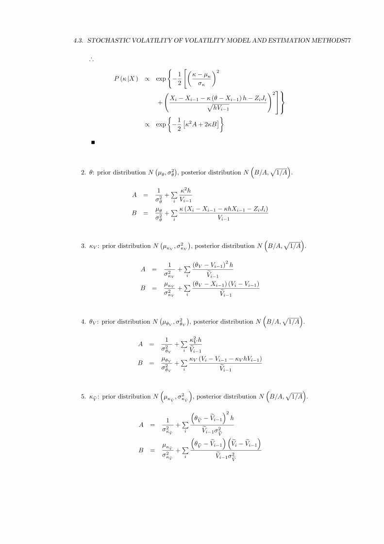
4.3. STOCHASTIC VOLATILITY OF VOLATILITYMODEL AND ESTIMATIONMETHODS77
∴
P (κ |X ) ∝ exp
−1
2
[(κ− µκσκ
)2
+
(Xi −Xi−1 − κ (θ −Xi−1)h− ZiJi√
hVi−1
)2
∝ exp
−1
2
[κ2A+ 2κB
]
2. θ: prior distribution N(µθ, σ
2θ
), posterior distribution N
(B/A,
√1/A
).
A =1
σ2θ
+∑i
κ2h
Vi−1
B =µθσ2θ
+∑i
κ (Xi −Xi−1 − κhXi−1 − ZiJi)Vi−1
3. κV : prior distribution N(µκV , σ
2κV
), posterior distribution N
(B/A,
√1/A
).
A =1
σ2κV
+∑i
(θV − Vi−1)2h
Vi−1
B =µκVσ2κV
+∑i
(θV −Xi−1) (Vi − Vi−1)
Vi−1
4. θV : prior distribution N(µθV , σ
2θV
), posterior distribution N
(B/A,
√1/A
).
A =1
σ2θV
+∑i
κ2V h
Vi−1
B =µθVσ2θV
+∑i
κV (Vi − Vi−1 − κV hVi−1)
Vi−1
5. κV : prior distribution N(µκV , σ
2κV
), posterior distribution N
(B/A,
√1/A
).
A =1
σ2κV
+∑i
(θV − Vi−1
)2
h
Vi−1σ2V
B =µκVσ2κV
+∑i
(θV − Vi−1
)(Vi − Vi−1
)Vi−1σ2
V

78 CHAPTER 4. STOCHASTIC VOLATILITY OF VOLATILITY
6. θV : prior distribution N(µθV , σ
2θV
), posterior distribution N
(B/A,
√1/A
).
A =1
σ2θV
+∑i
κ2V h
Vi−1σ2V
B =µθVσ2θV
+∑i
κV
(Vi − Vi−1 − κV hVi−1
)Vi−1σ2
V
7. σV can be simulated by random walk Metropolis algorithm.
8. J : prior Bernoulli(hλ0), posterior Bernoulli(
AA+B
)
A = hλ0 exp
−1
2
[Xi −Xi−1 − κ (θ −Xi−1)h− Zi√
hVi−1
]2
B = (1− hλ0) exp
−1
2
[Xi −Xi−1 − κ (θ −Xi−1)h√
hVi−1
]2
Proof. The posterior distribution is obtained by the following way:
∵
f (X |J ) ∝ exp
−1
2
[Xi −Xi−1 − κ (θ −Xi−1)h− ZiJi√
hVi−1
]2
∴
g (J |X ) =f (X |J ) g (J)∑f (X |J ) g (J)
=
(A
A+B
)J (1− A
A+B
)1−J
9. hλ0: prior distribution Beta(α0, β0), posterior distribution Beta(A,B).
A = α0 +∑i
Ji
B = β0 + n−∑i
Ji
Proof. The posterior distribution is obtained by the following way:
f (hλ0 |J ) ∝ f (J |hλ0 ) f(hλ0)
∝ (hλ0)
∑iJi (1− hλ0)
n−∑
iJ
(hλ0)α0−1
(1− hλ0)β0−1
= (hλ0)α0+∑
iJi−1
(1− hλ0)β0+n−
∑iJ−1

4.3. STOCHASTIC VOLATILITY OF VOLATILITYMODEL AND ESTIMATIONMETHODS79
10. Z: prior distribution N(µJ , σ
2J
), posterior distribution N
(B/A,
√1/A
).
A =1
σ2J
+∑i
JihVi−1
B =µJσ2J
+∑i
Ji (Xi −Xi−1 − κh (θ −Xi−1))
hVi−1
11. µJ : prior distribution N(µµJ , σ
2µJ
), posterior distribution N
(B/A,
√1/A
).
A =1
σ2µJ
+n
σ2J
B =µµJσ2µJ
+∑i
Ziσ2J
12. σ2J : prior distribution InvGamma (α, β), posterior distribution InvGamma (A,B) .
A = α+n
2
B = β +∑i
(Zi − µJ)2
2
Proof. The posterior distribution is obtained in the following way:
f(σ2J |Z
)∝ f
(Z∣∣σ2J
)f(σ2
J)
∝ 1
(σ2J)n/2
exp
(−1
2
∑i
(Zi − µJ)2
σ2J
)(σ2J
)−α−1exp
(− β
σ2J
)
=(σ2J
)−(α+n2 )−1
exp
−β +∑i
(Zi−µJ )2
2
σ2J
13. Update V and V :
P(Vi
∣∣∣V−i, X, V, Z, J,Θ)P(Vi
∣∣∣V−i, X, V , Z, J,Θ)The appendix shows the result of MCMC on the simulated data for a reduced
model.
dXt = κXtdt+√VtdW
Xt ,
dVt = κV (θV − Vt) dt+ VtVtdWVt ,
dVt = κV
(θV − Vt
)dt+ σVtdW
Vt .

80 CHAPTER 4. STOCHASTIC VOLATILITY OF VOLATILITY
Generating random variables in C++
MCMC algorithm needs to simulate random variables from different distributions.
Commonly used distributions include normal, truncated normal, beta and inverse
gamma distributions. In this study, we adopted the C function on [13]: use ’ran1’
to generate uniform random variables, ’gasdev’to generate normal random variables
and ’expdev’to generate exponential random variables.
In the following part, I will show the code for the inverse Gamma distribution. Let
us firstly recall that the probability density function of inverse Gamma distribution
is
f (x;α, β) =βα
Γ (α)(x)−α−1
exp
(−βx
)The easiest way to simulate inverse Gamma variables is to firstly simulate a
Gamma random variable and use the following property.
If X ∼ Gamma(α,
1
β
), then
1
X∼ InvGamma (α, β)
The algorithm to generate a Gamma random variable is recorded in Robert and
Casella (1999), (Page 47 and 55). Here ’betarv’ is the function for beta random
variables.
//Inverse Gamma
//Reference: C.P.Robert and G.Casella ’Monte Carlo Statistical Methods’
double invgamma(double aa, double bb, long seed)
double y,z,gamma;
double b,c,u,v,w;
//generate Gamma(aa,1)
if (aa<1)
y=betarv(aa,1-aa,seed); //betarv generates beta r.v.
z=expdev(&seed);
gamma=y*z;
//if
if (aa==1) gamma=expdev(&seed);
if (aa>1)
b=aa-1;
c=(12*aa-3)/4;
for(;;)
u=ran1(&seed);
v=ran1(&seed);

4.3. STOCHASTIC VOLATILITY OF VOLATILITYMODEL AND ESTIMATIONMETHODS81
w=u*(1-u);
y=sqrt(c/w)*(u-0.5);
gamma=b+y;
if(gamma<=0) continue;
z=64*v*v*w*w*w;
if(z<=1-2*y*y/gamma || 2*(b*log(gamma/b)-y)>=log(z)) break;
//for
//else
gamma/=bb;
//make it inversegamma (aa,bb)
return 1/gamma;
//function
4.3.2 Maximum likelihood estimation via closed-form likeli-hood expansion
Aït-Sahalia (2008) [2] proposed a method to find out the explicit form of a log-
likelihood function, which is the key to the maximum likelihood estimation. Let the
log likelihood function be approximated by a power series in the time interval ∆:
l(J)X (∆, x|x0; θ) = −m
2ln (2π∆)−Dv (x; θ) +
C(−1)X (x|x0; θ)
∆+
J∑k=0
C(k)X (x|x0; θ)
∆k
k!
The coeffi cients C(k)X solve the equation
f(k−1)X (x|x0) = 0
where
f(−2)X (x|x0) = −2C
(−1)X (x|x0; θ)−
∑i,j
vi,j(x)∂C
(−1)X (x|x0; θ)
∂xi
∂C(−1)X (x|x0; θ)
∂xj
f(−1)X (x|x0) = −G(0)
X (x|x0; θ)−∑i,j
vi,j(x)∂C
(−1)X (x|x0; θ)
∂xi
∂C(0)X (x|x0; θ)
∂xj
for k ≥ 1
f(k−1)X (x|x0) = C
(k)X (x|x0; θ)− 1
k
∑i,j
vi,j(x)∂C
(−1)X (x|x0; θ)
∂xi
∂C(k)X (x|x0; θ)
∂xj
−G(k)X (x|x0; θ)
The functions G(k)X (x|x0; θ) are specified by Aït-Sahalia (2008).
To better determine the coeffi cients C(k)X , one may consider the expansion C(jk,k)
X

82 CHAPTER 4. STOCHASTIC VOLATILITY OF VOLATILITY
in (x− x0) of each coeffi cient C(k)X . Let i = (i1, i2, ..., im) denote a vector of integers
and define Ik = i = (i1, i2, ..., im) ∈ Nm : 0 ≤ tr[i] ≤ jk so that the form of C(jk,k)X
is
C(jk,k)X (x|x0) =
∑i∈Ik
β(k)i (x0) (x1 − x01)
i1 ... (xm − x0m)im
The coeffi cients β(k)i (x0) are determined by setting the expansion f
(jk,k−1)X of
f(k−1)X to zero. In particular, when tr[i] = 2, we obtain the equation
∑tr[i]=2
β(−1)i (x0) (x1 − x01)
i1 ... (xm − x0m)im = −1
2(x− x0)
Tυ−1 (x0) (x− x0)
where υ (x) is the infinitesimal variance-covariance matrix of the process.
Fit Heston model to VIX and VIX option data
We applied this method to fit a Heston model to the VIX data between 03 Jan 2011
and 15 Apr 2011 with Black-Scholes implied volatility exacted from in-the-money
VIX option as the proxy volatility. The following figures compare the histogram of
the realized increments of the log VIX series and the increments determined by the
fitted Heston model. It is obvious that they do not share the same properties.
We experienced diffi culty to apply this method to the SVV model for S&P500 due
to the huge number of equations need to solve.
realized increments of the log VIX series

4.3. STOCHASTIC VOLATILITY OF VOLATILITYMODEL AND ESTIMATIONMETHODS83
increments determined by the fitted Heston model
4.3.3 Calibration
The third method we have tried is the calibration method. This technique can be
implemented to all the models considered.
The object of calibration is to find out the optimal parameters for the underlying
asset model which can best match the observed derivative prices. Mathematically the
idea can be expressed as:
minΘ
∥∥Ctheoretical(Θ)− Creal∥∥
VIX and VIX option
Let us firstly look at VIX and VIX derivatives. Kaeck and Alexander (2010) has found
an improvement of the model for VIX after incorporating the volatility of volatility
risk. But there is still a question left: what kind of structure the dynamic of the
volatility of VIX should take? We consider the following models for log VIX:
1. Jump volatility of volatility model:
d ln(V IX)t = (a− b ln(V IX)t) dt+
√VtdWt
dVt =(a− bVt
)dt+
√VtdJt
Jt ∼ NIG(α, β, µ, δ)

84 CHAPTER 4. STOCHASTIC VOLATILITY OF VOLATILITY
2. Heston model:
d ln(V IX)t = (a− b ln(V IX)t) dt+
√VtdW
V IXt
dVt =(a− bVt
)dt+ σ
√VtdW
Vt
3. Zeeman’s market model:
d ln(V IX)t = (a− b ln(V IX)t) dt+
√VtdW
V IXt
dVt =(a− bVt + cV 3
t
)dt+ σ
√VtdW
Vt
We calibrated all the three models to the VIX options with different strikes and
maturities. The following figures show the realized VIX option prices in 03 Jan 2011
and theoretical VIX option prices obtained by calibrated models. A clear improvement
can be seen if we model the volatility of the log VIX as a jump process, especially for
out-of-money options.
realized and theoretical option prices in 04 Jan 2011
Now let us try another date, 04 Feb 2011. The jump volatility of volatility model
still outperforms the other two models when price the out-of-money options, however
underperforms when price highly in-the-money options.

4.3. STOCHASTIC VOLATILITY OF VOLATILITYMODEL AND ESTIMATIONMETHODS85
SPX and SPX option
We consider the following SVV models for S&P500 series.
1. Jump stochastic volatility of volatility model:
d lnSt = (a− b lnSt) dt+ VtdWSt
dVt =(aV − bV Vt
)dt+ VtdW
Vt
dVt =(aV − bV Vt
)dt+ σVtdJt
Jt ∼ NIG(α, β, µ, δ),⟨WX ,WV
⟩= ρ
2. BM stochastic volatility of volatility model:
d lnSt = (a− b lnSt) dt+ VtdWSt
dVt =(aV − bV Vt
)dt+ VtdW
Vt
dVt =(aV − bV Vt
)dt+ σVtdW
Vt
Jt ∼ NIG(α, β, µ, δ)
3. Stochastic volatility model:
d lnSt = (a− b lnSt) dt+ VtdWSt
dVt =(aV − bV Vt
)dt+ σVtdW
Vt

86 CHAPTER 4. STOCHASTIC VOLATILITY OF VOLATILITY
Surprisingly, we found out that the adding stochastic volatility of volatility worsens
the option pricing.
realized and theoretical option prices in 04 Jan 2011
realized and theoretical option prices in 18 Feb 2011

4.4. CONCLUSION 87
4.4 Conclusion
This essay studied two kinds of volatility of volatility: i) the volatility of the volatility
of stock return; ii) the volatility of VIX. The stochastic volatility of volatility model
for S&P500 index involves three SDEs whereas the SVV model for VIX is in fact a
SV model.
The essay also tried three methods to fit SVV models to real data: i) Markov
Chain Monte Carlo; ii) Maximum likelihood estimation via closed-form likelihood
expansion; iii) Calibration. The last method was eventually worked out for all the
models and reveals the influence of incorporating volatility of volatility risk on the
option evaluation. Surprisingly, the SVV model fails to improve the effi ciency of
option pricing significantly.

88 CHAPTER 4. STOCHASTIC VOLATILITY OF VOLATILITY

Bibliography
[1] T.G. Andersen, L. Benzoni (2008). Realized Volatility. Working Paper.
[2] Y. Aït-Sahalia (2008). Closed-Form Likelihood Expansions for Multivariate Dif-
fusions. Annals of Statistics, 36, 906-937.
[3] Y. Aït-Sahalia, R. Kimmel (2007). Maximum Likelihood Estimation of Stochastic
Volatility Models. Journal of Financial Economics, 83, 413-452.
[4] Y. Aït-Sahalia, L. Zhang and P. Mykland (2011). Ultra High Frequency Volatility
Estimation with Dependent Microstructure Noise. Journal of Econometrics, 160,
190-203.
[5] S. Asmussen, P.W. Glynn (2007). Stochastic simulation: algorithms and analysis.
Springer.
[6] P. Carr, R. Lee (2007). Realized Volatility and Variance: Options via Swaps. Risk.
May.
[7] P. Carr, R. Lee (2009). Volatility Derivatives. Annual Review of Financ. Econ.
1:1—21.
[8] B. Dupire. (1994). Pricing with a Smile. Risk Magazine.
[9] H.S.B. Herath, P. Kumar (2002). The Jackknife Estimator for Estimating the
Volatility of Volatility of a Stock. Corporate Finance Review. Vol 7, No. 3, 13-21.
[10] S.D.H. Hsu, B.M. Murray (2007). On the volatility of volatility. Physica A: Sta-
tistical Mechanics and its Applications, vol. 380. 366-376.
[11] L. Ingber, J.K. Wilson (1999). Volatility of volatility of financial markets, Mathl.
Computer Modelling 29, 39-57.
[12] A. Kaeck, C. Alexander (2010). VIX Dynamics with Stochastic Volatility of
Volatility. Working Paper.
[13] W.H. Press, S.A. Teukolsky, W.T. Vetterling, and B.P. Flannery (1992). Numer-
ical Recipes in C: The Art of Scientific Computing, Second Edition. Cambridge
University Press.
89

90 BIBLIOGRAPHY
[14] C.P. Robert and G. Casella (1999). Monte Carlo Statistical Methods. Springer
text in Statistics.
[15] A. Swishchuk (2010). Stochastic Volatility and Change of Time: Overview. Pre-
sentation Slides.
[16] CBOE (2009). The CBOE Volatility Index - VIX.
www.cboe.com/micro/vix/vixwhite.pdf

BIBLIOGRAPHY 91
Appendix
The following shows the result of MCMC on the data simulated by the 3-SDE
model. The algorithm starts from the true value and include 50,000 iterations.
κ :
κV :

92 BIBLIOGRAPHY
θV :
κV :

BIBLIOGRAPHY 93
θV :
σ :

94 BIBLIOGRAPHY
Likelihood :