ece531 lecture 7: bayesian estimation and an...
TRANSCRIPT
ECE531 Lecture 7: Bayesian Estimation
ECE531 Lecture 7: Bayesian Estimation and an
Introduction to Non-Random Parameter Estimation
D. Richard Brown III
Worcester Polytechnic Institute
16-March-2011
Worcester Polytechnic Institute D. Richard Brown III 16-March-2011 1 / 35
ECE531 Lecture 7: Bayesian Estimation
Introduction
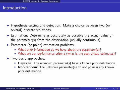
Hypothesis testing and detection: Make a choice between two (orseveral) discrete situations.
Estimation: Determine as accurately as possible the actual value ofthe parameter(s) from the observation (usually continuous).
Parameter (or point) estimation problems: What prior information do we have about the parameter(s)? What are our performance criteria (what is the cost of bad estimates)?
Two basic approaches: Bayesian: The unknown parameter(s) have a known prior distribution. Non-random: The unknown parameter(s) do not possess any known
prior distribution.
Worcester Polytechnic Institute D. Richard Brown III 16-March-2011 2 / 35
ECE531 Lecture 7: Bayesian Estimation
Mathematical Model for Estimation
parameter space observation space
estimator
probabilisticmodel
estimate
Λ Y
pθ(y)
θ(y)
θ
θ
y
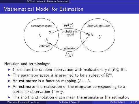
Notation and terminology:
Y denotes the random observation with realizations y ∈ Y ⊆ Rn.
The parameter space Λ is assumed to be a subset of Rm.
An estimator is a function mapping Y 7→ Λ. An estimate is a realization of the estimator corresponding to a
particular observation Y = y. The shorthand notation θ can mean the estimate or the estimator.Worcester Polytechnic Institute D. Richard Brown III 16-March-2011 3 / 35
ECE531 Lecture 7: Bayesian Estimation
Example 1
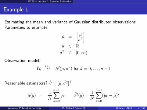
Estimating the mean and variance of Gaussian distributed observations.Parameters to estimate:
θ =
[µσ2
]
µ ∈ R
σ2 ∈ [0,∞)
Observation model:
Yki.i.d.∼ N (µ, σ2) for k = 0, . . . , n − 1
Reasonable estimators? θ = [µ, σ2]⊤
µ(y) =1
N
n−1∑
k=0
yk σ2(y) =1
N
n−1∑
k=0
(yk − µ)2
Worcester Polytechnic Institute D. Richard Brown III 16-March-2011 4 / 35
ECE531 Lecture 7: Bayesian Estimation
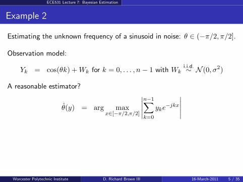
Example 2
Estimating the unknown frequency of a sinusoid in noise: θ ∈ (−π/2, π/2].
Observation model:
Yk = cos(θk) + Wk for k = 0, . . . , n − 1 with Wki.i.d.∼ N (0, σ2)
A reasonable estimator?
θ(y) = arg maxx∈[−π/2,π/2]
∣∣∣∣∣
n−1∑
k=0
yke−jkx
∣∣∣∣∣
Worcester Polytechnic Institute D. Richard Brown III 16-March-2011 5 / 35
ECE531 Lecture 7: Bayesian Estimation
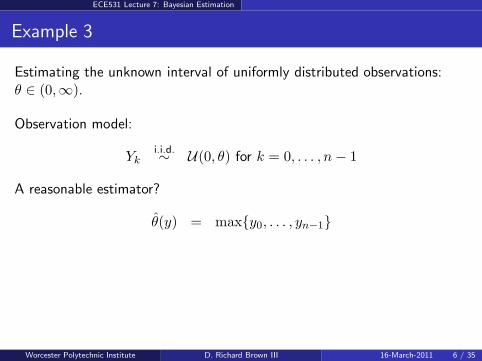
Example 3
Estimating the unknown interval of uniformly distributed observations:θ ∈ (0,∞).
Observation model:
Yki.i.d.∼ U(0, θ) for k = 0, . . . , n − 1
A reasonable estimator?
θ(y) = maxy0, . . . , yn−1
Worcester Polytechnic Institute D. Richard Brown III 16-March-2011 6 / 35
ECE531 Lecture 7: Bayesian Estimation
Cost Assignments and Conditional Risk
Intuitively, an optimal estimator will find the “best” guess of the trueparameter θ.
The solution to this problem depends on how we define “best” andhow we penalize any deviation from “best”.
Cost assignment: Cθ(θ) : Λ × Λ 7→ R is the cost of the parameterestimate θ ∈ Λ given the true parameter θ ∈ Λ.
Conditional risk of estimator θ(y) when the true parameter is θ:
Rθ(θ) := E[
Cθ(θ(Y )) | θ]
=
∫
YCθ(θ(y))pθ(y) dy
Worcester Polytechnic Institute D. Richard Brown III 16-March-2011 7 / 35
ECE531 Lecture 7: Bayesian Estimation
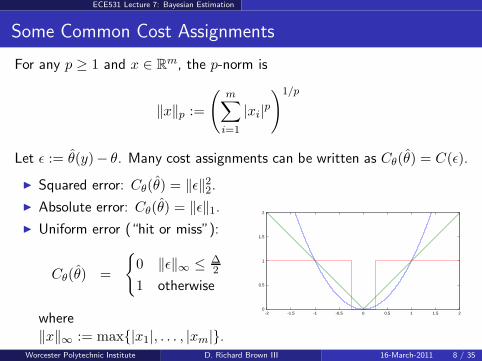
Some Common Cost Assignments
For any p ≥ 1 and x ∈ Rm, the p-norm is
‖x‖p :=
(m∑
i=1
|xi|p
)1/p
Let ǫ := θ(y)− θ. Many cost assignments can be written as Cθ(θ) = C(ǫ).
Squared error: Cθ(θ) = ‖ǫ‖22.
Absolute error: Cθ(θ) = ‖ǫ‖1.
Uniform error (“hit or miss”):
Cθ(θ) =
0 ‖ǫ‖∞ ≤ ∆2
1 otherwise
where‖x‖∞ := max|x1|, . . . , |xm|.
0
0.5
1
1.5
2
-2 -1.5 -1 -0.5 0 0.5 1 1.5 2
Worcester Polytechnic Institute D. Richard Brown III 16-March-2011 8 / 35
ECE531 Lecture 7: Bayesian Estimation
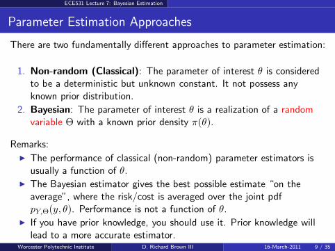
Parameter Estimation Approaches
There are two fundamentally different approaches to parameter estimation:
1. Non-random (Classical): The parameter of interest θ is consideredto be a deterministic but unknown constant. It not possess anyknown prior distribution.
2. Bayesian: The parameter of interest θ is a realization of a randomvariable Θ with a known prior density π(θ).
Remarks:
The performance of classical (non-random) parameter estimators isusually a function of θ.
The Bayesian estimator gives the best possible estimate “on theaverage”, where the risk/cost is averaged over the joint pdfpY,Θ(y, θ). Performance is not a function of θ.
If you have prior knowledge, you should use it. Prior knowledge willlead to a more accurate estimator.
Worcester Polytechnic Institute D. Richard Brown III 16-March-2011 9 / 35

ECE531 Lecture 7: Bayesian Estimation
The Bayesian Philosophy
We assume that the unknown parameter(s) are random with a known priordistribution Θ ∼ π(θ). The average/Bayes risk of estimator θ(y) is then
r(θ) = E[RΘ(θ)]
=
∫
ΛRθ(θ)π(θ) dθ
=
∫
Λ
∫
YCθ(θ(y))pθ(y)π(θ) dy dθ
=
∫
Y
∫
ΛCθ(θ(y))pθ(y)π(θ) dθ dy.
This should look similar to composite Bayesian hypothesis testing where
r(ρ, π) =
∫
Yρ⊤(y)
∫
XC(x)px(y)π(x) dx dy
where C(x) = [C0,x, . . . , CM−1,x]⊤. Our intuition here was to specify adecision rule that selected the index with “minimum commodity cost”.
Worcester Polytechnic Institute D. Richard Brown III 16-March-2011 10 / 35
ECE531 Lecture 7: Bayesian Estimation
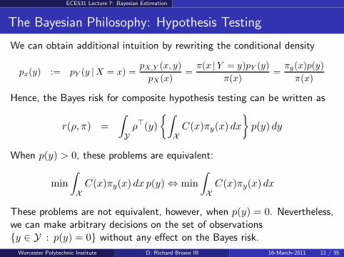
The Bayesian Philosophy: Hypothesis Testing
We can obtain additional intuition by rewriting the conditional density
px(y) := pY (y |X = x) =pX,Y (x, y)
pX(x)=
π(x |Y = y)pY (y)
π(x)=
πy(x)p(y)
π(x)
Hence, the Bayes risk for composite hypothesis testing can be written as
r(ρ, π) =
∫
Yρ⊤(y)
∫
XC(x)πy(x) dx
p(y) dy
When p(y) > 0, these problems are equivalent:
min
∫
XC(x)πy(x) dx p(y) ⇔ min
∫
XC(x)πy(x) dx
These problems are not equivalent, however, when p(y) = 0. Nevertheless,we can make arbitrary decisions on the set of observationsy ∈ Y : p(y) = 0 without any effect on the Bayes risk.
Worcester Polytechnic Institute D. Richard Brown III 16-March-2011 11 / 35
ECE531 Lecture 7: Bayesian Estimation
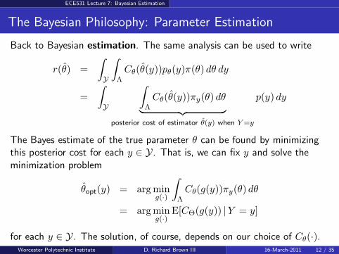
The Bayesian Philosophy: Parameter Estimation
Back to Bayesian estimation. The same analysis can be used to write
r(θ) =
∫
Y
∫
ΛCθ(θ(y))pθ(y)π(θ) dθ dy
=
∫
Y
∫
ΛCθ(θ(y))πy(θ) dθ
︸ ︷︷ ︸
posterior cost of estimator θ(y) when Y =y
p(y) dy
The Bayes estimate of the true parameter θ can be found by minimizingthis posterior cost for each y ∈ Y. That is, we can fix y and solve theminimization problem
θopt(y) = arg ming(·)
∫
ΛCθ(g(y))πy(θ) dθ
= arg ming(·)
E[CΘ(g(y)) |Y = y]
for each y ∈ Y. The solution, of course, depends on our choice of Cθ(·).Worcester Polytechnic Institute D. Richard Brown III 16-March-2011 12 / 35
ECE531 Lecture 7: Bayesian Estimation
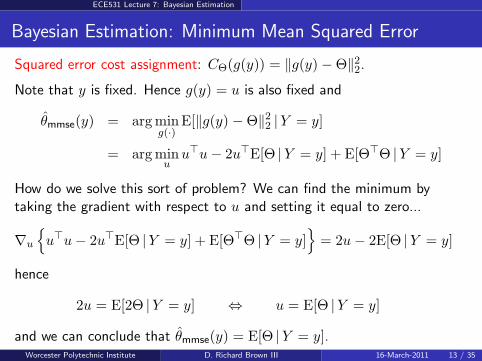
Bayesian Estimation: Minimum Mean Squared Error
Squared error cost assignment: CΘ(g(y)) = ‖g(y) − Θ‖22.
Note that y is fixed. Hence g(y) = u is also fixed and
θmmse(y) = arg ming(·)
E[‖g(y) − Θ‖22 |Y = y]
= arg minu
u⊤u − 2u⊤E[Θ |Y = y] + E[Θ⊤Θ |Y = y]
How do we solve this sort of problem? We can find the minimum bytaking the gradient with respect to u and setting it equal to zero...
∇u
u⊤u − 2u⊤E[Θ |Y = y] + E[Θ⊤Θ |Y = y]
= 2u − 2E[Θ |Y = y]
hence
2u = E[2Θ |Y = y] ⇔ u = E[Θ |Y = y]
and we can conclude that θmmse(y) = E[Θ |Y = y].Worcester Polytechnic Institute D. Richard Brown III 16-March-2011 13 / 35
ECE531 Lecture 7: Bayesian Estimation
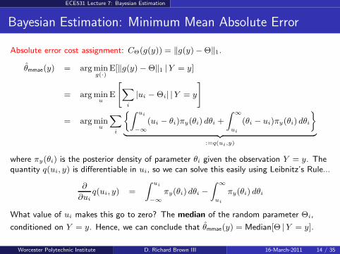
Bayesian Estimation: Minimum Mean Absolute Error
Absolute error cost assignment: CΘ(g(y)) = ‖g(y) − Θ‖1.
θmmae(y) = arg ming(·)
E[‖g(y) − Θ‖1 |Y = y]
= arg minu
E
"X
i
|ui − Θi| |Y = y
#
= arg minu
X
i
Z ui
−∞
(ui − θi)πy(θi) dθi +
Z∞
ui
(θi − ui)πy(θi) dθi
ff
| z
:=q(ui,y)
where πy(θi) is the posterior density of parameter θi given the observation Y = y. The
quantity q(ui, y) is differentiable in ui, so we can solve this easily using Leibnitz’s Rule...
∂
∂uiq(ui, y) =
Z ui
−∞
πy(θi) dθi −
Z∞
ui
πy(θi) dθi
What value of ui makes this go to zero? The median of the random parameter Θi,
conditioned on Y = y. Hence, we can conclude that θmmae(y) = Median[Θ |Y = y].
Worcester Polytechnic Institute D. Richard Brown III 16-March-2011 14 / 35
ECE531 Lecture 7: Bayesian Estimation
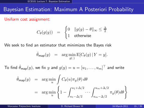
Bayesian Estimation: Maximum A Posteriori Probability
Uniform cost assignment:
Cθ(g(y)) =
0 ‖g(y) − θ‖∞ ≤ ∆2
1 otherwise
We seek to find an estimator that minimizes the Bayes risk
θmap(y) = arg ming(·)
E[Cθ(g) |Y = y].
To find θmap(y), we fix y and g(y) = u = [u1, . . . , um]⊤ and write
θmap(y) = arg minu
∫
Cθ(u)πy(θ) dθ
= arg minu
1 −
∫ u1+∆/2
u1−∆/2· · ·
∫ um+∆/2
um−∆/2πy(θ)dθ
Worcester Polytechnic Institute D. Richard Brown III 16-March-2011 15 / 35

ECE531 Lecture 7: Bayesian Estimation
Bayesian Estimation: Maximum A Posteriori Probability
We can’t take this much further without two additional assumptions: (A1)the posterior density πy(θ) is smooth and (A2) ∆ is small. Under theseassumptions, we can write
∫ u1+∆/2
u1−∆/2· · ·
∫ um+∆/2
um−∆/2πy(θ)dθ ≈ ∆mπy(θ)|θ=u.
Hence we have
θmap(y) = arg minu
1 − ∆mπy(u) .
Since ∆ > 0, we can discard the ∆m term and use our usual tricks to write
θmap(y) = arg maxu
πy(u).
Remarks:
θmap(y) = Mode[Θ |Y = y]. The solution is usually unique (but doesn’t have to be).
Worcester Polytechnic Institute D. Richard Brown III 16-March-2011 16 / 35
ECE531 Lecture 7: Bayesian Estimation
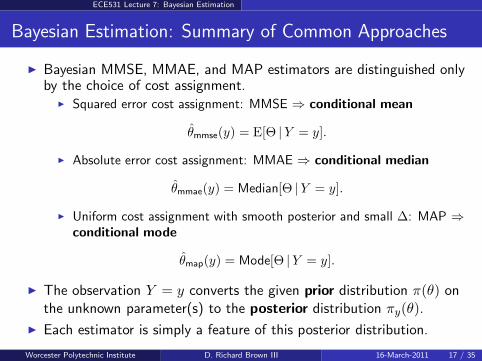
Bayesian Estimation: Summary of Common Approaches
Bayesian MMSE, MMAE, and MAP estimators are distinguished onlyby the choice of cost assignment.
Squared error cost assignment: MMSE ⇒ conditional mean
θmmse(y) = E[Θ |Y = y].
Absolute error cost assignment: MMAE ⇒ conditional median
θmmae(y) = Median[Θ |Y = y].
Uniform cost assignment with smooth posterior and small ∆: MAP ⇒conditional mode
θmap(y) = Mode[Θ |Y = y].
The observation Y = y converts the given prior distribution π(θ) onthe unknown parameter(s) to the posterior distribution πy(θ).
Each estimator is simply a feature of this posterior distribution.
Worcester Polytechnic Institute D. Richard Brown III 16-March-2011 17 / 35

ECE531 Lecture 7: Bayesian Estimation
Bayesian Estimation: Summary of Common Approaches
prior
posterior
mmaemapmmse
Worcester Polytechnic Institute D. Richard Brown III 16-March-2011 18 / 35

ECE531 Lecture 7: Bayesian Estimation
Performance of Bayesian MMSE Estimator
MMSE = E[
‖Θ − θmmse(Y )‖22
]
where the expectation is evaluated with respect to the joint pdf pY,Θ(y, θ).
MMSE =
∫ ∫
‖θ − E[Θ |Y = y]‖22 pY,Θ(y, θ) dy dθ
=
∫ ∫
‖θ − E[Θ |Y = y]‖22 πy(θ) dθ p(y) dy
=
∫ ∫∑
i
(θi − E[Θi |Y = y])2 πy(θ) dθ p(y) dy
=
∫∑
i
var(Θi |Y = y) p(y) dy
=
∫
trace cov(Θ |Y = y) p(y) dy
where trace(·) is the sum of the diagonal elements of a matrix.Worcester Polytechnic Institute D. Richard Brown III 16-March-2011 19 / 35

ECE531 Lecture 7: Bayesian Estimation
Bayesian Estimation for the Linear Gaussian Model
An important special case that covers many common estimation scenariosis the linear Gaussian signal model. In this model, the vector observation isgiven as
Y = HΘ + W
where the observation Y ∈ Rn, the “mixing matrix” H ∈ R
n×m is known,the unknown parameter vector Θ ∈ R
m is distributed as N (µΘ,ΣΘ), andthe unknown noise vector W ∈ R
n is distributed as N (0,ΣW ). Unlessotherwise specified, we always assume the noise and the unknownparameters are independent of each other.
To specify a MMSE/MMAE/MAP Bayesian estimator, we are going toneed to compute posterior distribution πy(θ). Note that we can’t just write
Θ = H−1(Y − W )
since H may not be invertible (or even square). Hence, finding πy(θ)involves a little bit of work...
Worcester Polytechnic Institute D. Richard Brown III 16-March-2011 20 / 35
ECE531 Lecture 7: Bayesian Estimation
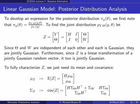
Linear Gaussian Model: Posterior Distribution Analysis
To develop an expression for the posterior distribution πy(θ), we first note
that πy(θ) =pY,Θ(y,θ)
pY (y) . To find the joint distribution pY,Θ(y, θ) let
Z =
[YΘ
]
=
[H II 0
] [ΘW
]
Since Θ and W are independent of each other and each is Gaussian, theyare jointly Gaussian. Furthermore, since Z is a linear transformation of ajointly Gaussian random vector, it too is jointly Gaussian.
To fully characterize Z, we just need its mean and covariance:
µZ := E[Z] =
[HµΘ
µΘ
]
ΣZ := cov[Z] =
[HΣΘH⊤ + ΣW HΣΘ
ΣΘH⊤ ΣΘ
]
Worcester Polytechnic Institute D. Richard Brown III 16-March-2011 21 / 35
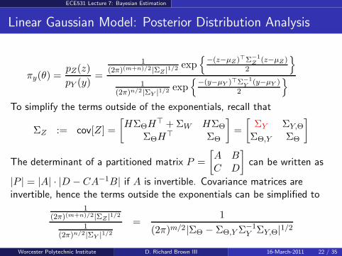
ECE531 Lecture 7: Bayesian Estimation
Linear Gaussian Model: Posterior Distribution Analysis
πy(θ) =pZ(z)
pY (y)=
1(2π)(m+n)/2|ΣZ |1/2 exp
−(z−µZ)⊤Σ−1
Z (z−µZ )2
1(2π)n/2|ΣY |1/2 exp
−(y−µY )⊤Σ−1
Y (y−µY )2
To simplify the terms outside of the exponentials, recall that
ΣZ := cov[Z] =
[HΣΘH⊤ + ΣW HΣΘ
ΣΘH⊤ ΣΘ
]
=
[ΣY ΣY,Θ
ΣΘ,Y ΣΘ
]
The determinant of a partitioned matrix P =
[A BC D
]
can be written as
|P | = |A| · |D − CA−1B| if A is invertible. Covariance matrices areinvertible, hence the terms outside the exponentials can be simplified to
1(2π)(m+n)/2|ΣZ |1/2
1(2π)n/2|ΣY |1/2
=1
(2π)m/2|ΣΘ − ΣΘ,Y Σ−1Y ΣY,Θ|1/2
Worcester Polytechnic Institute D. Richard Brown III 16-March-2011 22 / 35
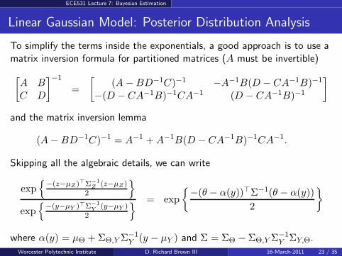
ECE531 Lecture 7: Bayesian Estimation
Linear Gaussian Model: Posterior Distribution Analysis
To simplify the terms inside the exponentials, a good approach is to use amatrix inversion formula for partitioned matrices (A must be invertible)
[A BC D
]−1
=
[(A − BD−1C)−1 −A−1B(D − CA−1B)−1
−(D − CA−1B)−1CA−1 (D − CA−1B)−1
]
and the matrix inversion lemma
(A − BD−1C)−1 = A−1 + A−1B(D − CA−1B)−1CA−1.
Skipping all the algebraic details, we can write
exp
−(z−µZ )⊤Σ−1Z (z−µZ)
2
exp
−(y−µY )⊤Σ−1Y (y−µY )
2
= exp
−(θ − α(y))⊤Σ−1(θ − α(y))
2
where α(y) = µΘ + ΣΘ,Y Σ−1Y (y − µY ) and Σ = ΣΘ − ΣΘ,Y Σ−1
Y ΣY,Θ.Worcester Polytechnic Institute D. Richard Brown III 16-March-2011 23 / 35

ECE531 Lecture 7: Bayesian Estimation
Linear Gaussian Model: Posterior Distribution Analysis
Putting it all together, we have the posterior distribution
πy(θ) =1
(2π)m/2|Σ|1/2exp
−(θ − α(y))⊤Σ−1(θ − α(y))
2
where α(y) = µΘ + ΣΘ,Y Σ−1Y (y − µY ) and Σ = ΣΘ − ΣΘ,Y Σ−1
Y ΣY,Θ with
ΣΘ,Y = cov(Θ, Y ) = E[
(Θ − µΘ)(HΘ + W − HµΘ)⊤]
= ΣΘH⊤
ΣY,Θ = Σ⊤Θ,Y = HΣΘ
ΣY = cov(Y, Y ) = HΣΘH⊤ + ΣW
µY = E[HΘ + W ] = HµΘ
What can we say about the distribution of the random parameter Θconditioned on the observation Y = y?
Worcester Polytechnic Institute D. Richard Brown III 16-March-2011 24 / 35
ECE531 Lecture 7: Bayesian Estimation
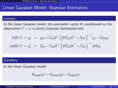
Linear Gaussian Model: Bayesian Estimators
Lemma
In the linear Gaussian model, the parameter vector Θ conditioned on the
observation Y = y is jointly Gaussian distributed with
E[Θ |Y = y] = µΘ + ΣΘH⊤(
HΣΘH⊤ + ΣW
)−1(y − HµΘ)
cov[Θ |Y = y] = ΣΘ − ΣΘH⊤(
HΣΘH⊤ + ΣW
)−1HΣΘ
Corollary
In the linear Gaussian model
θmmse(y) = θmmae(y) = θmap(y)
Worcester Polytechnic Institute D. Richard Brown III 16-March-2011 25 / 35
ECE531 Lecture 7: Bayesian Estimation
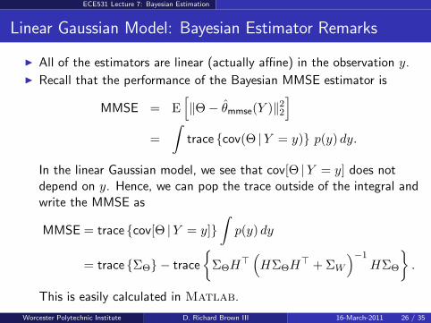
Linear Gaussian Model: Bayesian Estimator Remarks
All of the estimators are linear (actually affine) in the observation y.
Recall that the performance of the Bayesian MMSE estimator is
MMSE = E[
‖Θ − θmmse(Y )‖22
]
=
∫
trace cov(Θ |Y = y) p(y) dy.
In the linear Gaussian model, we see that cov[Θ |Y = y] does notdepend on y. Hence, we can pop the trace outside of the integral andwrite the MMSE as
MMSE = trace cov[Θ |Y = y]
∫
p(y) dy
= trace ΣΘ − trace
ΣΘH⊤(
HΣΘH⊤ + ΣW
)−1HΣΘ
.
This is easily calculated in Matlab.
Worcester Polytechnic Institute D. Richard Brown III 16-March-2011 26 / 35
ECE531 Lecture 7: Bayesian Estimation
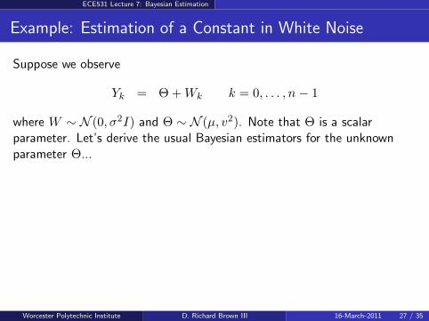
Example: Estimation of a Constant in White Noise
Suppose we observe
Yk = Θ + Wk k = 0, . . . , n − 1
where W ∼ N (0, σ2I) and Θ ∼ N (µ, v2). Note that Θ is a scalarparameter. Let’s derive the usual Bayesian estimators for the unknownparameter Θ...
Worcester Polytechnic Institute D. Richard Brown III 16-March-2011 27 / 35
ECE531 Lecture 7: Bayesian Estimation
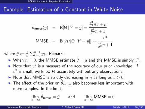
Example: Estimation of a Constant in White Noise
θmmse(y) = E[Θ |Y = y] =v2
σ2 ny + µv2
σ2 n + 1
MMSE = E [var[Θ |Y = y]] =v2
v2
σ2 n + 1
where y := 1n
∑n−1k=0 yk. Remarks:
When n = 0, the MMSE estimate θ = µ and the MMSE is simply v2. Note that v2 is a measure of the accuracy of our prior knowledge. If
v2 is small, we know Θ accurately without any observations. Note that MMSE is strictly decreasing in n as long as v > 0. The effect of the prior on θmmse also becomes less important with
more samples. In the limit
limn→∞
θmmse = y and limn→∞
MMSE = 0
Worcester Polytechnic Institute D. Richard Brown III 16-March-2011 28 / 35

ECE531 Lecture 7: Bayesian Estimation
Example: Estimation of Signal Amplitude in Colored Noise
Suppose now that we observe
Yk = Θsk + Wk k = 0, . . . , n − 1
where s = [s0, . . . , sn−1] is known, W ∼ N (0,Σ), and Θ ∼ N (µ, v2).Note that Θ is a scalar parameter. Let’s derive the usual Bayesianestimators for the unknown parameter Θ...
Worcester Polytechnic Institute D. Richard Brown III 16-March-2011 29 / 35
ECE531 Lecture 7: Bayesian Estimation
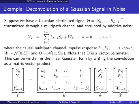
Example: Deconvolution of a Gaussian Signal in Noise
Suppose we have a Gaussian distributed signal Θ = [S0, . . . , SL−1]⊤
transmitted through a multipath channel and corrupted by additive noise:
Yk =
L−1∑
ℓ=0
hk−ℓSℓ + Wk k = 0, . . . , n − 1
where the causal multipath channel impulse response h0, h1, . . . is known,W ∼ N (0,Σ), and Θ ∼ N (µ,ΣΘ). Note that Θ is a vector parameter.This can be written in the linear Gaussian form by writing the convolutionas a matrix-vector product:
Y0
Y1...
Yn−1
︸ ︷︷ ︸
Y
=
h0 0 . . . 0h1 h0 . . . 0...
.... . .
...hn−1 hn−2 . . . h(n − L)
︸ ︷︷ ︸
H
S0
S1...
SL−1
︸ ︷︷ ︸
Θ
+
W0
W1...
WL−1
︸ ︷︷ ︸
W
Worcester Polytechnic Institute D. Richard Brown III 16-March-2011 30 / 35
ECE531 Lecture 7: Bayesian Estimation
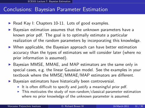
Conclusions: Bayesian Parameter Estimation
Read Kay I: Chapters 10-11. Lots of good examples.
Bayesian estimation assumes that the unknown parameters have aknown prior pdf. The goal is to optimally estimate a particularrealization of the random parameters by incorporating this knowledge.
When applicable, the Bayesian approach can have better estimationaccuracy than the types of estimators we will consider later (where noprior information is assumed).
Bayesian MMSE, MMAE, and MAP estimators are the same only inspecial cases, e.g. the linear Gaussian model. See the examples in yourtextbook where the MMSE/MMAE/MAP estimators are different.
Bayesian estimators have historically been controversial. It is often difficult to specify and justify a meaningful prior pdf. This motivates the study of non-random/classical parameter estimation
where no prior knowledge of the unknown parameter is assumed.
Worcester Polytechnic Institute D. Richard Brown III 16-March-2011 31 / 35
ECE531 Lecture 7: Bayesian Estimation
Introduction to Non-Random Parameter Estimation
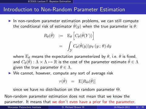
In non-random parameter estimation problems, we can still computethe conditional risk of estimator θ(y) when the true parameter is θ:
Rθ(θ) := Eθ
[
Cθ(θ(Y ))]
=
∫
YCθ(θ(y))pY (y ; θ) dy
where Eθ means the expectation parameterized by θ, i.e. θ is fixed,and Cθ(θ) : Λ × Λ 7→ R is the cost of the parameter estimate θ ∈ Λgiven the true parameter θ ∈ Λ.
We cannot, however, compute any sort of average risk
r(θ) = E[RΘ(θ)]
since we have no distribution on the random parameter Θ.
Non-random parameter estimation does not mean that we know theparameter. It means that we don’t even have a prior for the parameter.
Worcester Polytechnic Institute D. Richard Brown III 16-March-2011 32 / 35
ECE531 Lecture 7: Bayesian Estimation
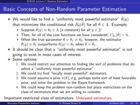
Basic Concepts of Non-Random Parameter Estimation
We would like to find a “uniformly most powerful estimator” θ(y)
that minimizes the conditional risk Rθ(θ) for all θ ∈ Λ. Example: Suppose θ(y) ≡ θ0 ∈ Λ (a constant) for all y ∈ Y. Then, for all of the cost functions we have considered, Cθ0
(θ) = 0. When the true parameter θ = θ1 6= θ0, however, the estimator
θ(y) ≡ θ1 outperforms θ(y) = θ0 when θ = θ1.
It should be clear that a “uniformly most powerful estimator” is notgoing to exist in most cases of interest.
Some options:1. We could restrict our attention to finding the sort of problems that do
admit a “uniformly most powerful estimator”.2. We could try find “locally most powerful” estimators.3. We could assume a prior π(θ), e.g. perhaps some sort of least favorable
prior, and solve the problem in the Bayes framework.4. We could keep the problem non-random but place restrictions on the
class of estimators that we are willing to consider.
Important restricted class of estimators: Unbiased estimators.Worcester Polytechnic Institute D. Richard Brown III 16-March-2011 33 / 35

ECE531 Lecture 7: Bayesian Estimation
Option 4: Consider Only Unbiased Estimators
A reasonable restriction on the class of estimators that we are willing toconsider is the class of unbiased estimators.
Definition
An estimator θ(y) is unbiased if
Eθ
[
θ(Y )]
= θ
for all θ ∈ Λ.
Remarks:
This class excludes trivial estimators like θ(y) ≡ θ0. Under the squared-error cost assignment, estimators in this class
Rθ(θ) = Eθ
h
‖θ − θ(Y )‖22
i
=X
i
Eθi
h
(θi(Y ) − θi)2i
=X
i
varθi
h
θi(Y )i
Optimal approach: minimum variance unbiased (MVU) estimators
Worcester Polytechnic Institute D. Richard Brown III 16-March-2011 34 / 35
ECE531 Lecture 7: Bayesian Estimation
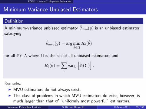
Minimum Variance Unbiased Estimators
Definition
A minimum-variance unbiased estimator θmvu(y) is an unbiased estimatorsatisfying
θmvu(y) = arg minθ∈Ω
Rθ(θ)
for all θ ∈ Λ where Ω is the set of all unbiased estimators and
Rθ(θ) =∑
i
varθi
[
θi(Y )]
.
Remarks:
MVU estimators do not always exist.
The class of problems in which MVU estimators do exist, however, ismuch larger than that of “uniformly most powerful” estimators.
Worcester Polytechnic Institute D. Richard Brown III 16-March-2011 35 / 35