overview multiple imputation for multilevel data bayesian ... · pdf filebayesian estimation...

Multiple Imputation for Multilevel Data

Craig K. Enders Brian T. Keller University of California - Los Angeles Department of Psychology

Work supported by IES award R305D150056

Overview

Bayesian estimation for MLMs

Univariate multiple imputation

Joint model imputation

Fully conditional specification

Incomplete categorical variables

Software examples

Session 2

Session 1

Why Imputation?

Dedicated multilevel programs restricts maximum likelihood estimation to incomplete outcomes

Multilevel SEM software is more flexible but typically imposes normality on incomplete predictors and may perform poorly in some cases

Imputation is flexible (e.g., mixtures of categorical and continuous variables are no problem)

Model Notation

Two-level model with observation i nested in cluster j (e.g., student i in school j )

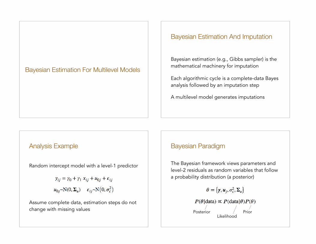
Bayesian Estimation For Multilevel Models

Bayesian Estimation And Imputation

Bayesian estimation (e.g., Gibbs sampler) is the mathematical machinery for imputation

Each algorithmic cycle is a complete-data Bayes analysis followed by an imputation step

A multilevel model generates imputations

Analysis Example

Random intercept model with a level-1 predictor

Assume complete data, estimation steps do not change with missing values

Bayesian Paradigm

The Bayesian framework views parameters and level-2 residuals as random variables that follow a probability distribution (a posterior)

LikelihoodPriorPosterior

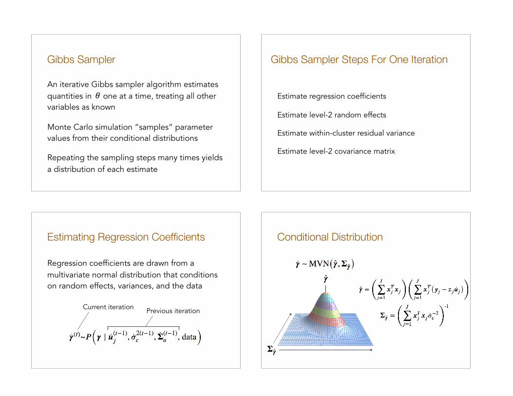
Gibbs Sampler

An iterative Gibbs sampler algorithm estimates quantities in one at a time, treating all other variables as known

Monte Carlo simulation “samples” parameter values from their conditional distributions

Repeating the sampling steps many times yields a distribution of each estimate

Gibbs Sampler Steps For One Iteration

Estimate regression coefficients

Estimate level-2 random effects

Estimate within-cluster residual variance

Estimate level-2 covariance matrix

Estimating Regression Coefficients

Regression coefficients are drawn from a multivariate normal distribution that conditions on random effects, variances, and the data

Current iteration Previous iteration

Conditional Distribution

Level-2 random effects are drawn from a multivariate normal distribution that conditions on the coefficients, variances, and the data

Estimating Level-2 Random Effects

Updated estimatesPrevious iteration


Estimating The Residual Variance

The within-cluster residual variance is drawn from an inverse Wishart distribution that conditions on the previous coefficients, random effects, level-2 covariance matrix, and the data


Estimating Level-2 Covariance Matrix

The level-2 covariance matrix is sampled from an inverse Wishart distribution that conditions on the previous coefficients, random effects, residual variance, and the data

Iteration t is complete, start anew at iteration t + 1


Univariate Multiple Imputation

Multilevel Imputation

Imputation uses a model with an incomplete variable regressed on complete variables

Bayesian estimation steps are applied to the filled-in data from the previous iteration

Model parameters and level-2 residuals define a distribution from which imputations are sampled

Analysis And Imputation Models

Random intercept analysis model with an incomplete predictor

Random intercept imputation model with the incomplete predictor as the outcome

Estimate coefficients

Estimate random effects

Estimate residual variance

Estimate covariance matrix

Gibbs Sampler Steps

Update imputations

Complete-data Bayes estimation

Imputation step

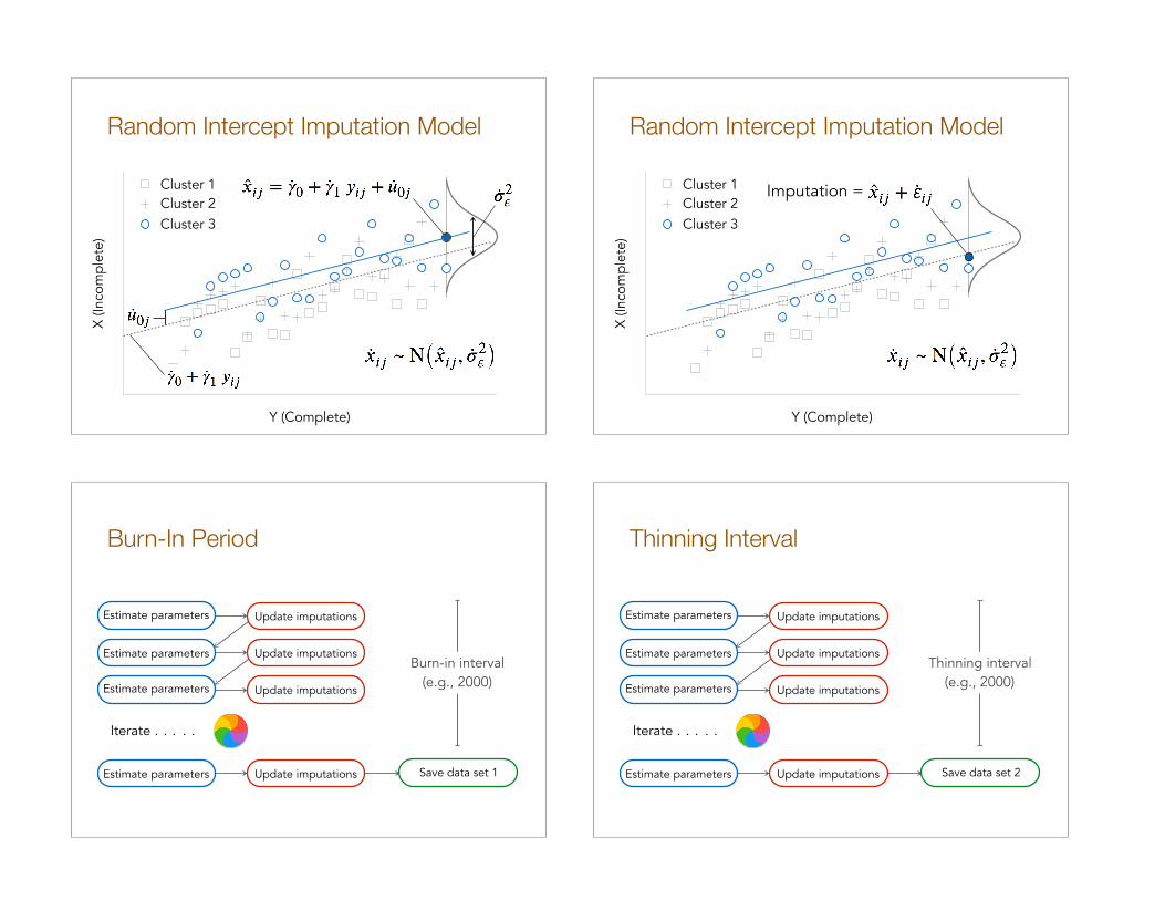
Distribution Of Missing Values

A normal distribution generates imputations, with center equal to the predicted value for observation i in cluster j and spread equal to the within-cluster residual variance

Random Intercept Imputation Model

X (I

ncom

plet

e)

Y (Complete)

Cluster 1Cluster 2Cluster 3

Random Intercept Imputation ModelX

(Inc

ompl

ete)

Y (Complete)


Random Intercept Imputation Model

X (I

ncom

plet

e)

Y (Complete)


Imputation =

Burn-In Period

Burn-in interval (e.g., 2000)

Iterate . . . . .

Estimate parameters Update imputations



Save data set 1Estimate parameters Update imputations

Thinning Interval

Iterate . . . . .


Estimate parameters

Estimate parameters

Update imputations

Update imputations


Thinning interval (e.g., 2000)

Repeat Until Finished …

Iterate . . . . .


Estimate parameters

Estimate parameters

Update imputations

Update imputations


Thinning interval (e.g., 2000)

Analysis And Pooling

The analysis model is fit to each data set, and the arithmetic average of the M estimates is the multiple imputation point estimate

Pooling assumes a normal sampling distribution

Pooling Standard Errors

Average sampling variance

Variance across imputations

Standard error

Multivariate Missing Data

Joint model imputation uses multivariate regression to impute the set of missing variables

Fully conditional specification imputes variables one at a time in a sequence

Both are multilevel extensions of major single-level imputation frameworks

Multivariate Imputation With The Joint Modeling Framework

Joint Model Imputation

Two forms:

1) Multivariate regression model with incomplete variables regressed on complete variables

2) Empty model treating all variables as outcomes

Available in Mplus, MLwiN, and R packages (e.g., jomo, pan, mlmmm)

Random Intercept Analysis Model

Two-level random intercept analysis with continuous level-1 and level-2 predictors

All variables have missing data

Imputation Model

Covariance Structure

Level-1

?

Level-2

Imputation Step

Compatibility Of Imputation And Analysis

The imputation model is more flexible than the analysis model because it allows level-1 and level-2 covariance matrices to freely vary

The analysis model assumes a common slope

Imputations are appropriate for random intercept analyses that partition relations into within- and between-cluster parts

Compatible Analysis Models

Contextual effects analyses

Multilevel SEM

R Package jomo# load packages library (jomo)

# read raw data dat <- read.table("~/desktop/examples/ridata.csv", sep = ",") names(dat) = c("cluster", "av1", "av2", "y", "x","w") dat[dat == 999] <- NA

# jomo imputation set.seed(90291) dat$icept <- 1 l1miss <- c("y", "x") l2miss <- c("w") l1complete <- c("icept") l2complete <- c("icept") impdata <- jomo(dat[l1miss], Y2 = dat[l2miss], X = dat[l1complete], X2 = dat[l2complete], clus = dat$cluster, nburn = 2000, nbetween = 2000, nimp = 20, meth = "common")

Mplus data: file = ridata.csv; variable: names = cluster av1 av2 y x w; usevariables = av1 av2 y x w; missing = all(999); analysis: type = basic; bseed = 90291; data imputation: impute = y x w; ndatasets = 20; save = imp*.dat; thin = 1000; output: tech8;

Simulation Study

Random intercept model with 1000 replications

ICC = .25, medium effect sizes

30 clusters with 5 or 30 observations per cluster (i.e., N = 150 and 900)

15% MAR missing data on all analysis variables

20 imputations with R package jomo-40 -20 0 20

Complete Data Joint Model Imputation

-40 -20 0 20

Percentage Bias Percentage Bias

Intercept

L1 Slope

L2 Slope

Intercept Var.

Residual Var.

J = 30, nj = 5 J = 30, nj = 30

Random Slope Analysis Model

Two-level random slope analysis with continuous level-1 and level-2 predictors


Joint Model Limitations

Within-cluster covariances must preserve level-1 relations, including the random coefficients

The classic formulation of the joint model assumes a common covariance matrix at level-1

Imputation ignores random slope variation

Covariance Structure Revisited

Level-1

?

Level-2

Simulation Study

Random slope model with 1000 replications




20 imputations with R package jomo

-40 -20 0 20



Intercept

L1 Slope

L2 Slope

Intercept Var.

Residual Var.

Covariance

Slope Var.

-40 -20 0 20

J = 30, nj = 5 J = 30, nj = 30Brief Maximum Likelihood Detour

Mplus allows incomplete random slope predictors

Requires numerical integration and many latent variable products

Often yields severe bias

Percentage Bias

J = 30, nj = 30

Intercept

L1 Slope

L2 Slope

Intercept Var.

Residual Var.

Covariance

Slope Var.

-40 -20 0 20

Joint Modeling With Random Level-1 Covariance Matrices

Yucel (2011) extended the joint model to incorporate random level-1 covariance matrices

Available in the R package jomo

Currently limited to 2-level models


Level-1

?

Level-2

Limitation Of Random Covariance Matrices

The between-cluster covariance matrix preserves random intercept variation, while the within-cluster matrices preserve random slopes

Elements of in the analysis model depend on orthogonal sources of variation

Imputation assumes no correlation between the random intercepts and slopes


Level-1

?

Level-2

Intercept variation

Slope variation

R Package jomo# load packages library (jomo)

# read raw data dat <- read.table("~/desktop/examples/ridata.csv", sep = ",") names(dat) = c("cluster", "av1", "av2", "y", "x","w") dat[dat == 999] <- NA

# jomo imputation set.seed(90291) dat$icept <- 1 l1miss <- c("y", "x") l2miss <- c("w") l1complete <- c("icept") l2complete <- c("icept") impdata <- jomo(dat[l1miss], Y2 = dat[l2miss], X = dat[l1complete], X2 = dat[l2complete], clus = dat$cluster, nburn = 2000, nbetween = 2000, nimp = 20, meth = "random")

Simulation Study





20 imputations with R package jomo

-40 -20 0 20



Intercept

L1 Slope

L2 Slope

Intercept Var.

Residual Var.

Covariance

Slope Var.

-40 -20 0 20

J = 30, nj = 5 J = 30, nj = 30

Multivariate Imputation With Fully Conditional Specification

Fully Conditional Specification

Variable-by-variable imputation

Uses a series of univariate regression models with an incomplete variable regressed on complete and previously imputed variables

Available in R package mice (2-level models with continuous variables) and the Blimp application for MacOS, Windows, and Linux

Random Intercept Analysis Model

Two-level random intercept analysis with continuous level-1 and level-2 predictors


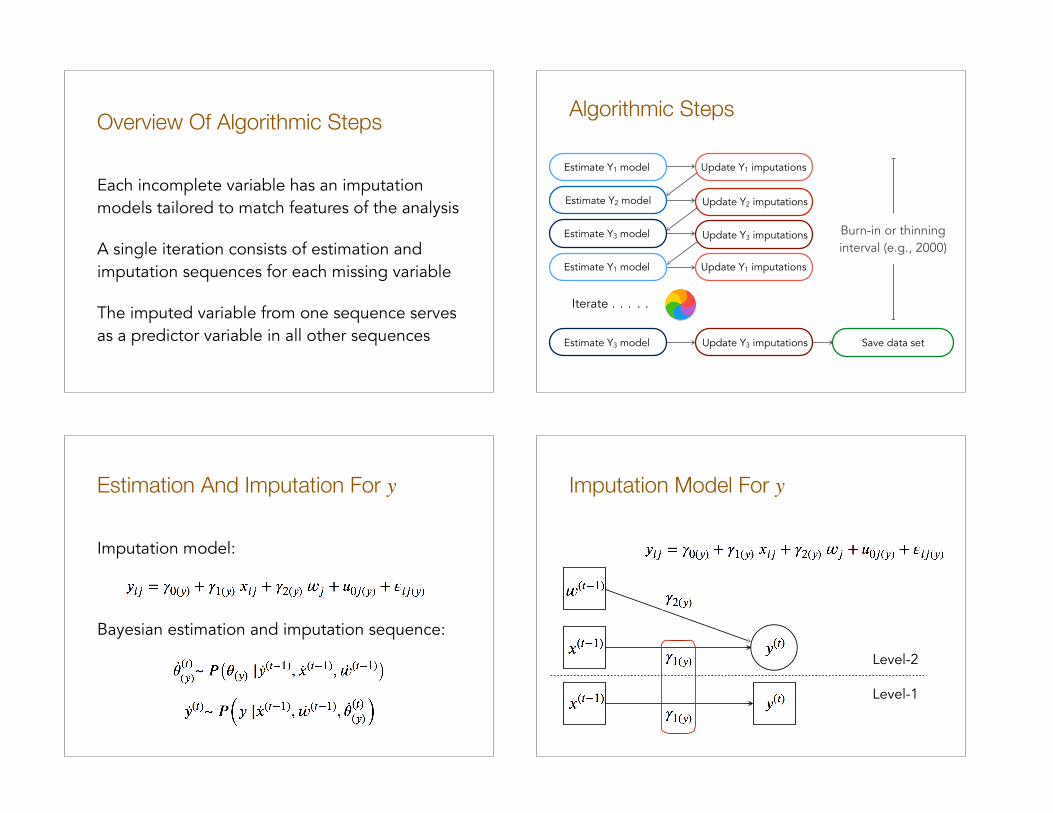
Overview Of Algorithmic Steps

Each incomplete variable has an imputation models tailored to match features of the analysis

A single iteration consists of estimation and imputation sequences for each missing variable

The imputed variable from one sequence serves as a predictor variable in all other sequences

Algorithmic Steps

Burn-in or thinning interval (e.g., 2000)

Estimate Y3 model

Update Y1 imputationsEstimate Y1 model


Update Y3 imputations

Save data set

Iterate . . . . .

Estimate Y1 model Update Y1 imputations


Estimation And Imputation For y

Imputation model:

Bayesian estimation and imputation sequence:

Imputation Model For y

Level-1

Level-2

Imputation Step For y Estimation And Imputation For x

Imputation model:


Imputation Model For x

Level-1

Level-2

Imputation Step For x

Estimation And Imputation For w

Imputation model:


Imputation Model For w

Level-1

Level-2

Imputation Step For w Blimp Syntax

DATA: ~/desktop/examples/ridata.csv; VARIABLES: cluster av1 av2 y x w; MISSING: 999; MODEL: cluster ~ y x w; NIMPS: 20; THIN: 2000; BURN: 2000; SEED: 90291; OUTFILE: ~/desktop/examples/imps.csv; OPTIONS: stacked noclmeans prior1;

Simulation Study

Random intercept model with 1000 replications




20 imputations with the Blimp application-40 -20 0 20

Complete Data Joint Model FCS

-40 -20 0 20


Intercept

L1 Slope

L2 Slope

Intercept Var.

Residual Var.

J = 30, nj = 5 J = 30, nj = 30

Limitations

The classic formulation of fully conditional specification assumes equal within- and between-cluster regression slopes

i.e., Equality constraints on the level-1 and level-2 model-implied covariance matrices

Not ideal for models that partition relations

Revisiting Models That Partition Variability

Contextual effects analyses

Multilevel SEM

Partitioned Imputation Model For y

Level-1

Level-2

Partitioned Imputation Model For x

Level-1

Level-2


Level-1

Level-2

Blimp Syntax

DATA: ~/desktop/examples/ridata.csv; VARIABLES: cluster av1 av2 y x w; MISSING: 999; MODEL: cluster ~ y x w; NIMPS: 20; THIN: 2000; BURN: 2000; SEED: 90291; OUTFILE: ~/desktop/example/imps.csv; OPTIONS: stacked clmeans prior1;

Random Slope Analysis Model

Two-level random slope analysis with continuous level-1 and level-2 predictors


Reversed Random Coefficients

Fully conditional specification uses “reversed random coefficients” to preserve random slope variation

Imputation treats x as a random predictor of y, and y as a random predictor of x

Reversed Coefficient Model For y

Level-1

Level-2

Reversed Coefficient Model For x

Level-1

Level-2


Level-1

Level-2

Blimp Syntax

DATA: ~/desktop/examples/rsdata.csv; VARIABLES: cluster av1 av2 y x w; MISSING: 999; MODEL: cluster ~ y:x w; NIMPS: 20; THIN: 2000; BURN: 2000; SEED: 90291; OUTFILE: ~/desktop/examples/imps.csv; OPTIONS: stacked clmeans prior1;

Simulation Study





20 imputations with the Blimp application-40 -20 0 20

Complete Data Joint Model FCS


Intercept

L1 Slope

L2 Slope

Intercept Var.

Residual Var.

Covariance

Slope Var.

-40 -20 0 20

J = 30, nj = 5 J = 30, nj = 30

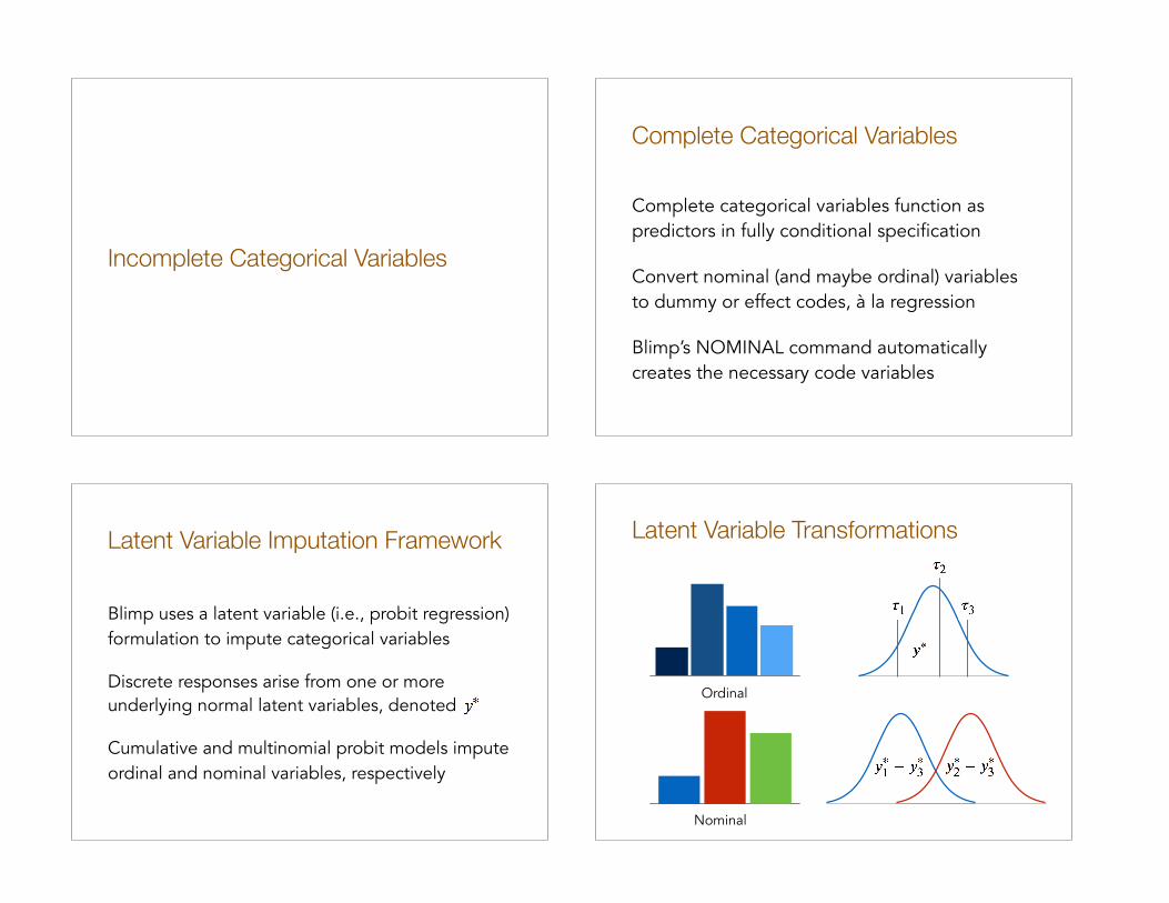
Incomplete Categorical Variables

Complete Categorical Variables

Complete categorical variables function as predictors in fully conditional specification

Convert nominal (and maybe ordinal) variables to dummy or effect codes, à la regression

Blimp’s NOMINAL command automatically creates the necessary code variables

Latent Variable Imputation Framework

Blimp uses a latent variable (i.e., probit regression) formulation to impute categorical variables

Discrete responses arise from one or more underlying normal latent variables, denoted

Cumulative and multinomial probit models impute ordinal and nominal variables, respectively

Latent Variable Transformations

Ordinal

Nominal

Latent Variable Scaling

Latent variable distributions are centered at a predicted value and have residual variance fixed at one for identification

Random Intercept Model


1

Threshold Parameters

Ordinal (or binary) variables with K response options require K - 1 threshold parameters

Thresholds are z-scores corresponding to the cumulative percentage of each response

Thresholds slice the continuous latent distribution into discrete response segments

Marginal Distribution Example

12%

50%

0

12%

38% 29% 21%

-1.17 .81

z-Score

79%

1 2 3 4

1 2 3 4

Multilevel Model Example


1

2

3

4

Complete-Data Bayesian Estimation

The Gibbs sampler first replaces discrete responses with latent variable scores

Threshold parameters (ordinal variables) are sampled using a Metropolis step

Bayesian estimation steps for normal data update parameters and level-2 residual terms for the underlying latent variable model

Gibbs Sampler Steps

Bayes estimation for normal variables




Estimate thresholds (ordinal)Draw latent scores

“Impute” discrete responses

Estimate thresholds Ordinal variables

Latent Scores For Ordinal Variables

A discrete response restricts the plausible range of the latent scores

e.g., a score of y = 2 must have a latent score located between the appropriate thresholds

The latent variable scores are drawn from a normal distribution truncated at the thresholds

Truncated Normal Draw | y = 2

1

2

3

4

Implausible latent score, reject draw

Truncated Normal Draw | y = 2

1

2

3

4

Plausible latent score, retain draw

Incomplete Ordinal Variables

Identical procedure as complete data, with imputations generated at the end of each Bayesian estimation sequence

Latent scores for missing cases are unbounded because the truncation points are unknown

Latent imputes are subsequently discretized using threshold parameters

Gibbs Sampler Steps

Update latent imputations

Bayes estimation for normal variables




Estimate thresholds (ordinal)Draw latent scores

Convert to discrete imputes

Estimate thresholds Ordinal variables

Impute missing latent scores

Replace discrete responses

Truncated Normal Draw | y = ?

Plausible latent imputation

Generating Discrete Imputes

1

3

4

2

Multinomial Probit Model

The multinomial model defines K latent variables representing the response strength of each category

K categories require K-1 latent variable difference scores

Category K is the reference

2

1

3

Example: 3-Category Nominal Variable

Latent Variable Distributions

Cluster 1Cluster 2

Latent Scores For Nominal Variables

A discrete response occurs when its latent response strength exceeds those of all other categories

Category membership implies a rank order and magnitude for the latent difference scores

An accept-reject algorithm draws latent scores until it obtains values that satisfy the constraints

Latent Variable Score Constraints

2

1

30


2

1

30


2

1

30

Incomplete Nominal Variables

Category membership is unknown

Latent difference scores for incomplete cases can take on any configuration of values

Discrete imputes are generated by applying the order and magnitude conditions

Latent Difference Score Imputations

?

?

?

```````

0


2

1

30


2

1

30


2

1

30

Blimp Syntax

DATA: ~/desktop/examples/rsdata.csv; VARIABLES: cluster av1 av2 y x w; MISSING: 999; MODEL: cluster ~ y x w; ORDINAL: y; NOMINAL: x w; NIMPS: 20; THIN: 2000; BURN: 2000; SEED: 90291; OUTFILE: ~/desktop/examples/imps.csv; OPTIONS: stacked clmeans prior1;

Two-Level Analysis Example

Download Information

The Blimp application for MacOS and Windows is freely available online (Linux by request)

www.appliedmissingdata.com/multilevel-imputation.html

The data and analysis scripts are also available

Motivating Example

Data from a cluster-randomized study investigating a novel math problem-solving curriculum

29 schools (level-2 units) were randomly assigned to an intervention or control condition

The average number of students (level-1 units) per school was 33.86, with a range of 13 to 61

Input DataVariable Description Missing Metric

school School identifier variable

condition Treatment code (0 = control, 1 = intervention) Nominal

esolpercent Percentage of English as second language * Numeric

student Student identifier

abilitylev Ability grouping (3-group classification) * Nominal

female Female dummy code Nominal

stanmath Standardized math test scores * Numeric

frlunch Lunch assistance dummy code * Nominal

efficacy Math self-efficacy rating scale * Ordinal

probsolve1 Math problem-solving score at baseline * Numeric

probsolve7 Math problem-solving score at final wave * Ordinal

Leve

l-1Le

vel-2

Analysis Model

The substantive analysis model predicts end-of-year problem-solving scores from intervention condition and pretest covariates

Blimp Syntax

DATA: ~/Desktop/Blimp Examples/Ex2Level.csv; VARIABLES: school condition esolpercent student abilitylev female stanmath frlunch efficacy probsolve1 probsolve7; ORDINAL: efficacy; NOMINAL: condition abilitylev female frlunch; MISSING: 999; MODEL: school ~ condition esolpercent abilitylev female stanmath frlunch efficacy probsolve1 probsolve7; NIMPS: 20; THIN: 2000; BURN: 2000; SEED: 90291; OUTFILE: ~/Desktop/Blimp Examples/Imps2Level.csv; OPTIONS: stacked nopsr csv clmean prior1 hov;

Import Data

Specify Imputation Model

Specify Algorithmic Options

Specify Output Options

Run Program

Pooling with R Package mitml

# Required packages library(mitml) library(lme4)

# Read data imputations <- read.csv("~/desktop/Blimp Examples/Imps2Level.csv", header = F) names(imputations) <- c("imputation", "school", "condition", “esolpercent", "student", "abilitylev", "female", "stanmath", "frlunch", “efficacy”, "probsolve1", "probsolve7") imputations$abilitylev <- factor(imputations$abilitylev)

# Analyze data and pool estimates model <- "probsolve7 ~ probsolve1 + efficacy + abilitylev + female + esolpercent + condition + (1|school)" implist <- as.mitml.list(split(imputations, imputations$imputation)) mlm <- with(implist, lmer(model, REML = F)) estimates <- testEstimates(mlm, var.comp = T, df.com = NULL)

# Display estimates estimates

mitml Output

Final parameter estimates and inferences obtained from 20 imputed data sets.

Estimate Std.Error t.value df p.value RIV (Intercept) 55.932 4.928 11.349 500.705 0.000 0.242 probsolve1 0.416 0.040 10.330 297.510 0.000 0.338 efficacy 0.721 0.273 2.641 157.466 0.005 0.532 abilitylev2 1.169 1.526 0.766 131.473 0.222 0.613 abilitylev3 2.843 1.680 1.693 185.041 0.046 0.472 female 0.324 0.733 0.442 284.297 0.329 0.349 esolpercent 0.063 0.042 1.525 4350.615 0.064 0.071 condition 4.779 1.931 2.475 2174.122 0.007 0.103

Estimate Intercept~~Intercept|school 18.582 Residual~~Residual 89.179 ICC|school 0.172

Unadjusted hypothesis test as appropriate in larger samples.

Centering Predictors

Centering is performed post-imputation because the means are unknown with missing data

Center variables at imputation-specific constants

Centering constants (e.g., grand or group mean)



# Read data imputations <- read.csv("~/Desktop/ex/Imps2Level.csv", header = F) names(imputations) <- c("imputation", "school", "condition", "esolpercent", "student", "abilitylev", "female", "stanmath", "frlunch", "efficacy", "probsolve1", "probsolve7")

# Create Dummy codes (Factor 1 is reference) imputations$abilitylev <- factor(imputations$abilitylev) dummyCodes <- model.matrix( ~ imputations$abilitylev) imputations$abilityleveD1 <- dummyCodes[,2] imputations$abilityleveD2 <- dummyCodes[,3]

# Create imputations as a list imputationList <- split(imputations, imputations$imputation)

Pooling with R Package mitml, Cont.

# Grand mean centering impListCent <- lapply(imputationList,function(dat) { # Variables needing centering vars <- c("esolpercent", "student", "female", "stanmath", "frlunch", "efficacy", "probsolve1","abilityleveD1", "abilityleveD2") # Get grand means mns <- colMeans(dat[,vars]) # Center dat[,vars] <- sweep(dat[,vars],2,mns) # Return data return(dat) })

# Create imputations as mitml List implistCent <- as.mitml.list(impListCent)

# Analyze data and pool estimates model <- "probsolve7 ~ probsolve1 + efficacy + abilitylev + female + esolpercent + condition + (1|school)" mlm <- with(implistCent, lmer(model, REML = F)) estimates <- testEstimates(mlm, var.comp = T, df.com = NULL)

Multiple Imputation Significance Tests

Pooling Covariance Matrices

Average covariance matrix

Variance across imputations

Average proportional increase in variance

Wald Test Statistic

Evaluating the Wald statistic to a chi-square (shown below) or F distribution gives a p-value

Wald based on pooled quantities

Inflation factor

Wald Test With mitml# Empty model model1 <- "probsolve7 ~ (1|school)"

mlm1 <- with(implist, lmer(model1, REML = F)) estimates1 <- testEstimates(mlm1, var.comp = T, df.com = NULL) estimates1

# Covariates only model2 <- "probsolve7 ~ probsolve1 + efficacy + abilitylev +

female + esolpercent + (1|school)" mlm2 <- with(implist, lmer(model2, REML = F)) estimates2 <- testEstimates(mlm2, var.comp = T, df.com = NULL)

estimates2

# Compare models with Wald test testModels(mlm2, mlm1, method = "D1")

Output

Model comparison calculated from 20 imputed data sets.

Combination method: D1

F.value df1 df2 p.value RIV

28.657 6 1615.839 0.000 0.347


First And Second Pass Test Statistics

Pass 1: Average likelihood ratio statistic

Pass 2: Average test statistic with likelihood evaluated at the pooled estimates

Meng And Rubin (1992) Test Statistic

The LRT can be evaluated against a chi-square (shown below) or F distribution

LRT based on pooled quantities

Inflation factor

Average proportional increase in variance

Likelihood Ratio Test With mitml

# Random intercept model model1 <- "probsolve7 ~ probsolve1 + efficacy + abilitylev + female + esolpercent + condition + (1|school)"

mlm1 <- with(implist, lmer(model1, REML = F)) estimates1 <- testEstimates(mlm1, var.comp = T, df.com = NULL) estimates1

# Random slope for self-efficacy model2 <- "probsolve7 ~ probsolve1 + efficacy + abilitylev + female + esolpercent + condition + (efficacy|school)" mlm2 <- with(implist, lmer(model2, REML = F)) estimates2 <- testEstimates(mlm2, var.comp = T, df.com = NULL)

estimates2

# Compare models with Meng and Rubin likelihood ratio test testModels(mlm2, mlm1, method = "D3")

Output

Model comparison calculated from 20 imputed data sets.

Combination method: D3

F.value df1 df2 p.value RIV

0.085 2 786.816 0.918 0.249

Three-Level Analysis Example

Motivating Example

Data from a cluster-randomized study investigating a math problem-solving curriculum

29 schools (level-3 units) were randomly assigned to an intervention or control condition

The average number of students (level-2 units) per school was 33.86, with a range of 13 to 61

Seven (approximately) monthly assessments with planned missing data and attrition

Input DataVariable Description Missing Metric

school School identifier variable

condition Treatment code (0 = control, 1 = intervention) Nominal

esolpercent Percentage of English as second language * Numeric

student Student identifier

abilitylev Ability grouping (3-group classification) * Nominal

female Female dummy code Nominal

stanmath Standardized math test scores * Numeric

frlunch Lunch assistance dummy code * Nominal

wave Assessment wave

time Months since baseline Numeric

condbytime Condition by time interaction Numeric

probsolve Math problem-solving score * Numeric

efficacy Math self-efficacy 6-point rating scale * Ordinal

Leve

l-1Le

vel-2

Leve

l-3

Analysis Model

The substantive analysis model examines the intervention by time interaction, controlling for covariates at each level

Blimp Syntax

DATA: ~/Desktop/Blimp Examples/Ex3Level.csv; VARIABLES: school condition esolpercent student abilitylev female stanmath frlunch wave time condbytime probsolve efficacy; ORDINAL: efficacy; NOMINAL: condition abilitylev female frlunch; MISSING: 999; MODEL: student school ~ condition esolpercent abilitylev female stanmath frlunch condbytime efficacy time:probsolve; NIMPS: 20; THIN: 2000; BURN: 2000; SEED: 90291; OUTFILE: ~/Desktop/Blimp Examples/Imps3Level.csv; OPTIONS: stacked nopsr csv clmean prior1 hov;

Import Data

Specify Imputation Model

Specify Algorithmic Options

Specify Output Options

Run Program



# Read data imputations <- read.csv("~/desktop/Blimp Examples/Imps3Level.csv", header = F) names(imputations) <- c("imputation", "school", "condition", “esolpercent”, "student", "abilitylev", "female", "stanmath", "frlunch", "wave", “time", "condbytime", “probsolve", "efficacy") imputations$abilitylev <- factor(imputations$abilitylev)

# Analyze data and pool estimates model <- "probsolve ~ efficacy + time + condbytime + abilitylev + female + esolpercent + condition + (time|student:school) + (time|school)" implist <- as.mitml.list(split(imputations, imputations$imputation)) mlm <- with(implist, lmer(model, REML = F)) estimates <- testEstimates(mlm, var.comp = T, df.com = NULL)

# Display estimates estimates

mitml Output


Estimate Std.Error t.value df p.value RIV (Intercept) 92.715 1.917 48.373 549.605 0.000 0.228 efficacy 0.765 0.144 5.326 56.231 0.000 1.388 time 0.686 0.172 3.985 934.853 0.000 0.166 condbytime 0.549 0.222 2.470 1995.448 0.007 0.108 abilitylev2 0.747 0.886 0.843 321.312 0.200 0.321 abilitylev3 6.974 0.967 7.210 441.810 0.000 0.262 female -0.530 0.439 -1.207 968.110 0.114 0.163 esolpercent 0.051 0.023 2.194 1003.065 0.014 0.160 condition 0.083 1.085 0.077 2741.808 0.469 0.091

mitml Output

Estimate Intercept~~Intercept|student:school 23.532 Intercept~~time|student:school 0.529 time~~time|student:school 0.131 Intercept~~Intercept|school 5.038 Intercept~~time|school -0.167

time~~time|school 0.255 Residual~~Residual 62.353 ICC|school 0.274 NA 0.075


Interaction terms can be rescaled to equal the product of deviation score variables

Centering Incomplete Product Terms

Centering constants (e.g., grand or group mean)



# Read data imputations <- read.csv("~/Desktop/ex/Imps3Level.csv", header = F) names(imputations) <- c("imputation", "school", "condition", "esolpercent", "student", "abilitylev", "female", "stanmath", "frlunch", "wave", "time", "condbytime", "probsolve", "efficacy") # Create Dummy codes (Factor 1 is reference) imputations$abilitylev <- factor(imputations$abilitylev) dummyCodes <- model.matrix( ~ imputations$abilitylev) imputations$abilityleveD1 <- dummyCodes[,2] imputations$abilityleveD2 <- dummyCodes[,3]

# Create imputations as a list imputationList <- split(imputations, imputations$imputation)

mitml Output


Estimate Std.Error t.value df p.value RIV (Intercept) 101.891 1.361 74.840 1398.955 0.000 0.132 efficacy 0.765 0.144 5.326 56.231 0.000 1.388 time 0.686 0.172 3.985 934.854 0.000 0.166 condbytime 0.549 0.222 2.470 1995.446 0.007 0.108 abilitylev2 0.747 0.886 0.843 321.312 0.200 0.321 abilitylev3 6.974 0.967 7.210 441.809 0.000 0.262 female -0.530 0.439 -1.207 968.111 0.114 0.163 esolpercent 0.051 0.023 2.194 1003.064 0.014 0.160 condition 3.380 1.462 2.312 20385.340 0.010 0.031

Pooling with R Package mitml, Cont.

# Centering impListCent <- lapply(imputationList,function(dat) { # Variables needing grand mean centering vars <- c("efficacy", "esolpercent", "female","abilityleveD1", "abilityleveD2") # Get grand means mns <- colMeans(dat[,vars]) # Grand Mean Center dat[,vars] <- sweep(dat[,vars],2,mns) ## Center interaction # Time centering constant timeC <- 6 # Condition constant condC <- 0 # Center Time dat$time <- dat$time - timeC # Center Condition dat$condition <- dat$condition - condC # Center condbytime dat$condbytime <- dat$condbytime - (dat$condition*timeC) - (dat$time*condC) + (condC*timeC) # Return data return(dat) })

# Analyze data and pool estimates model <- "probsolve ~ efficacy + time + condbytime + abilitylev + female + esolpercent + condition + (time|student:school) + (time|school)" implist <- as.mitml.list(impListCent)

overview multiple imputation for multilevel data bayesian ... · pdf filebayesian estimation...

Documents