bayesian estimation - · pdf fileintroduction bayesian estimation: the basics priors...
TRANSCRIPT
IntroductionBayesian estimation: the basics
PriorsEvaluating the posterior
Bayesian inference and model comparisonBayesian estimation in Dynare
Extensions
Dynamic Macro
Bayesian Estimation
Petr Sedlacek
Bonn University
Summer 2015
1 / 114
IntroductionBayesian estimation: the basics
PriorsEvaluating the posterior
Bayesian inference and model comparisonBayesian estimation in Dynare
Extensions
Overall plan
Motivation
Week 1: Use of computational tools, simple DSGE model X
Tools necessary to solve models and a solution method
Week 2: function approximation and numerical integration X
Week 3: theory of perturbation (1st and higher-order) X
Tools necessary for, and principles of, estimation
Week 4: Kalman filter and Maximum Likelihood estimation X
Week 5: principles of Bayesian estimation
2 / 114

IntroductionBayesian estimation: the basics
PriorsEvaluating the posterior
Bayesian inference and model comparisonBayesian estimation in Dynare
Extensions
Plan for today
Bayesian estimation: the basic ideas
extra information over ML: priors
main challenge: evaluating the posterior
Markov Chain Monte Carlo (MCMC)
practical issues: acceptance rate, diagnostics
implementation in Dynare
3 / 114
IntroductionBayesian estimation: the basics
PriorsEvaluating the posterior
Bayesian inference and model comparisonBayesian estimation in Dynare
Extensions
Frequentist vs. Bayesian viewsBayes’ rule
Bayesian estimation: basic concepts
4 / 114

IntroductionBayesian estimation: the basics
PriorsEvaluating the posterior
Bayesian inference and model comparisonBayesian estimation in Dynare
Extensions
Frequentist vs. Bayesian viewsBayes’ rule
Frequentist vs. Bayesian views
Frequentist view:
parameters are fixed, but unknown
likelihood is a sampling distribution for the data
realizations of observables YT
just one of many possible realizations from L(YT |Ψ)
inferences about Ψ
based on probabilities of particular YT for given Ψ
5 / 114
IntroductionBayesian estimation: the basics
PriorsEvaluating the posterior
Bayesian inference and model comparisonBayesian estimation in Dynare
Extensions
Frequentist vs. Bayesian viewsBayes’ rule
Frequentist vs. Bayesian views
Bayesian view:
observations, not parameters, are taken as given
Ψ are viewed as random
inference about Ψ
based on probabilities of Ψ conditional on data YT P(Ψ|YT )
probabilistic view of Ψ enables incorporation of prior beliefs
Sims (2007):“Bayesian inference is a way of thinking, not a basket of methods”
6 / 114
IntroductionBayesian estimation: the basics
PriorsEvaluating the posterior
Bayesian inference and model comparisonBayesian estimation in Dynare
Extensions
Frequentist vs. Bayesian viewsBayes’ rule
Bayes’ rule
1701-1761
7 / 114
IntroductionBayesian estimation: the basics
PriorsEvaluating the posterior
Bayesian inference and model comparisonBayesian estimation in Dynare
Extensions
Frequentist vs. Bayesian viewsBayes’ rule
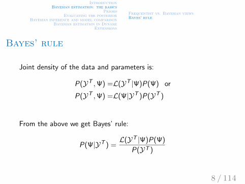
Bayes’ rule
Joint density of the data and parameters is:
P(YT ,Ψ) =L(YT |Ψ)P(Ψ) or
P(YT ,Ψ) =L(Ψ|YT )P(YT )
From the above we get Bayes’ rule:
P(Ψ|YT ) =L(YT |Ψ)P(Ψ)
P(YT )
8 / 114
IntroductionBayesian estimation: the basics
PriorsEvaluating the posterior
Bayesian inference and model comparisonBayesian estimation in Dynare
Extensions
Frequentist vs. Bayesian viewsBayes’ rule
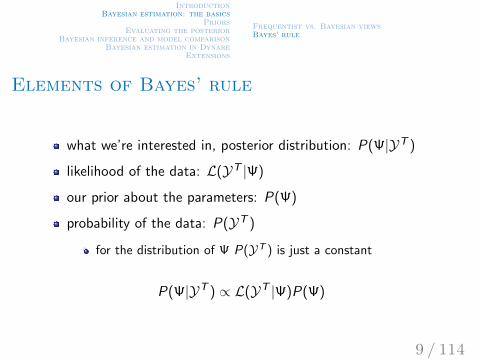
Elements of Bayes’ rule
what we’re interested in, posterior distribution: P(Ψ|YT )
likelihood of the data: L(YT |Ψ)
our prior about the parameters: P(Ψ)
probability of the data: P(YT )
for the distribution of Ψ P(YT ) is just a constant
P(Ψ|YT ) ∝ L(YT |Ψ)P(Ψ)
9 / 114

IntroductionBayesian estimation: the basics
PriorsEvaluating the posterior
Bayesian inference and model comparisonBayesian estimation in Dynare
Extensions
Frequentist vs. Bayesian viewsBayes’ rule
What is the challenge?
getting the posterior is typically not such a big deal
problem is that we often want to know more:
conditional expected values of a function of the posterior
like mean, variance, model etc.
10 / 114
IntroductionBayesian estimation: the basics
PriorsEvaluating the posterior
Bayesian inference and model comparisonBayesian estimation in Dynare
Extensions
Frequentist vs. Bayesian viewsBayes’ rule
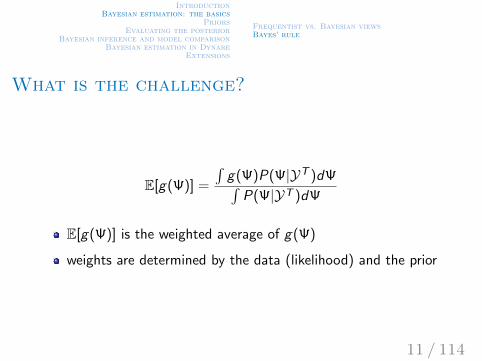
What is the challenge?
E[g(Ψ)] =
∫g(Ψ)P(Ψ|YT )dΨ∫
P(Ψ|YT )dΨ
E[g(Ψ)] is the weighted average of g(Ψ)
weights are determined by the data (likelihood) and the prior
11 / 114

IntroductionBayesian estimation: the basics
PriorsEvaluating the posterior
Bayesian inference and model comparisonBayesian estimation in Dynare
Extensions
Frequentist vs. Bayesian viewsBayes’ rule
What is the challenge?
we need to be able to evaluate the integral!
Special/Simple case:
we are able to draw Ψ from P(Ψ|YT )
can evaluate integral via Monte Carlo integration
you won’t be lucky enough to experience this case
12 / 114
IntroductionBayesian estimation: the basics
PriorsEvaluating the posterior
Bayesian inference and model comparisonBayesian estimation in Dynare
Extensions
Frequentist vs. Bayesian viewsBayes’ rule
Evaluating the posterior
Our situation:
we can calculate P(Ψ|YT ), but we cannot draw from it
Solutions:
numerical integration
Markov Chain Monte Carlo (MCMC) integration
What is the standard?
although numerical integration is fast and accurate
computational burden rises exponentially with dimension
suited for low-dimension problems
→ use MCMC methods
13 / 114

IntroductionBayesian estimation: the basics
PriorsEvaluating the posterior
Bayesian inference and model comparisonBayesian estimation in Dynare
Extensions
Priors
14 / 114
IntroductionBayesian estimation: the basics
PriorsEvaluating the posterior
Bayesian inference and model comparisonBayesian estimation in Dynare
Extensions
Idea of priors
summarize prior information
previous studies
data not used in estimation
pre-sample data
other countries etc.
don’t be too restrictive
more on prior selection in “extensions”
15 / 114
IntroductionBayesian estimation: the basics
PriorsEvaluating the posterior
Bayesian inference and model comparisonBayesian estimation in Dynare
Extensions
Priors
Most commonly used distributions:
normal
beta, support ∈ [0, 1]
persistence parameters
(inverted-) gamma, support ∈ (0,∞)
volatility parameters
uniform
16 / 114
IntroductionBayesian estimation: the basics
PriorsEvaluating the posterior
Bayesian inference and model comparisonBayesian estimation in Dynare
Extensions
Prior predictive analysis
check whether priors “make sense”
use the prior as the posterior
steady state?
impulse response functions?
17 / 114
IntroductionBayesian estimation: the basics
PriorsEvaluating the posterior
Bayesian inference and model comparisonBayesian estimation in Dynare
Extensions
Some terminology
Jeffreys prior
non-informative prior
improper vs. proper priors
improper prior is non-integrable (integral is ∞)
important to have proper distributions for model comparison
18 / 114
IntroductionBayesian estimation: the basics
PriorsEvaluating the posterior
Bayesian inference and model comparisonBayesian estimation in Dynare
Extensions
Some terminology
(natural) conjugate priors
family of prior distributions
after multiplication with the likelihood
produce a posterior of the same family
Minnesota (Litterman) prior
used in VARs for distribution of lags
19 / 114

IntroductionBayesian estimation: the basics
PriorsEvaluating the posterior
Bayesian inference and model comparisonBayesian estimation in Dynare
Extensions
Importance samplingMarkov Chain Monte CarloGibbs algorithmMetropolis-Hastings algorithmPractical issues with MH algorithm
Evaluating the posterior
20 / 114
IntroductionBayesian estimation: the basics
PriorsEvaluating the posterior
Bayesian inference and model comparisonBayesian estimation in Dynare
Extensions
Importance samplingMarkov Chain Monte CarloGibbs algorithmMetropolis-Hastings algorithmPractical issues with MH algorithm
Starting point
Aim is to be able to calculate something like
E[g(Ψ)] =
∫g(Ψ)P(Ψ|YT )dΨ∫
P(Ψ|YT )dΨ
we know how to calculate P(Ψ|YT )
but we cannot draw from it
the system is too large for numerical integration
21 / 114
IntroductionBayesian estimation: the basics
PriorsEvaluating the posterior
Bayesian inference and model comparisonBayesian estimation in Dynare
Extensions
Importance samplingMarkov Chain Monte CarloGibbs algorithmMetropolis-Hastings algorithmPractical issues with MH algorithm
Principle of posterior evaluation
We cannot draw from the “target” distribution, but
1. can draw from a different, “stand-in”, distribution
2. can evaluate both stand-in and target distributions
3. comparing the two, we can re-weigh the draw “cleverly”
22 / 114
IntroductionBayesian estimation: the basics
PriorsEvaluating the posterior
Bayesian inference and model comparisonBayesian estimation in Dynare
Extensions
Importance samplingMarkov Chain Monte CarloGibbs algorithmMetropolis-Hastings algorithmPractical issues with MH algorithm
Principle of posterior evaluation
the above procedure is the idea of “importance sampling”
MCMC methods effectively a version of importance sampling
traveling through the parameter space is more sophisticated
and or acceptance probability more sophisticated
23 / 114
IntroductionBayesian estimation: the basics
PriorsEvaluating the posterior
Bayesian inference and model comparisonBayesian estimation in Dynare
Extensions
Importance samplingMarkov Chain Monte CarloGibbs algorithmMetropolis-Hastings algorithmPractical issues with MH algorithm
A few simple examples
Problem:
we want to simulate x
x comes from truncated normal with
mean µ and variance σ2
and a < x < b
Solution:
1. draw y from N(µ, σ2)
2a. if y ∈ (a, b) then keep draw (accept) and go back to 1
2b. otherwise discard draw (reject) and go back to 1
24 / 114

IntroductionBayesian estimation: the basics
PriorsEvaluating the posterior
Bayesian inference and model comparisonBayesian estimation in Dynare
Extensions
Importance samplingMarkov Chain Monte CarloGibbs algorithmMetropolis-Hastings algorithmPractical issues with MH algorithm
A few simple examples
Problem:
want to draw x from F (x), but we cannot
we can sample from G (x) and f (x) ≤ cg(x) ∀xSolution:
1. sample y from G (y)
2. accept draw with probability f (y)cg(y) and go back to 1
Note:
acceptance rate higher for lower c
optimal c is c = supxf (x)g(x)
Metropolis-Hastings sampler (MCMC) is a generalization
25 / 114
IntroductionBayesian estimation: the basics
PriorsEvaluating the posterior
Bayesian inference and model comparisonBayesian estimation in Dynare
Extensions
Importance samplingMarkov Chain Monte CarloGibbs algorithmMetropolis-Hastings algorithmPractical issues with MH algorithm
Importance sampling
Main idea very similar to the previous example:
cannot draw from P(Ψ|YT )
but can draw from H(Ψ)
be smart in reweighing (accepting) the draws
26 / 114
IntroductionBayesian estimation: the basics
PriorsEvaluating the posterior
Bayesian inference and model comparisonBayesian estimation in Dynare
Extensions
Importance samplingMarkov Chain Monte CarloGibbs algorithmMetropolis-Hastings algorithmPractical issues with MH algorithm
Importance sampling
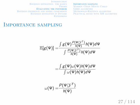
E[g(Ψ)] =
∫g(Ψ) P(Ψ|YT )
h(Ψ) h(Ψ)dΨ∫ P(Ψ|YT )h(Ψ) h(Ψ)dΨ
=
∫g(Ψ)ω(Ψ)h(Ψ)dΨ∫ω(Ψ)h(Ψ)dΨ
ω(Ψ) =P(Ψ|YT )
h(Ψ)
27 / 114

IntroductionBayesian estimation: the basics
PriorsEvaluating the posterior
Bayesian inference and model comparisonBayesian estimation in Dynare
Extensions
Importance samplingMarkov Chain Monte CarloGibbs algorithmMetropolis-Hastings algorithmPractical issues with MH algorithm
Importance sampling
Approximate the integral using MC integration:
E[g(Ψ)] ≈∑M
m=1 ω(Ψ(m))g(Ψ(m))∑Mm=1 ω(Ψ(m))
M is the number of draws from importance function h(Ψ)
28 / 114
IntroductionBayesian estimation: the basics
PriorsEvaluating the posterior
Bayesian inference and model comparisonBayesian estimation in Dynare
Extensions
Importance samplingMarkov Chain Monte CarloGibbs algorithmMetropolis-Hastings algorithmPractical issues with MH algorithm
Importance sampling
How to best choose h(.)?
we’d like h(.) to have fatter tails compared to f (.)
normal distribution has rather thin tails
→ often not a good importance function
29 / 114

IntroductionBayesian estimation: the basics
PriorsEvaluating the posterior
Bayesian inference and model comparisonBayesian estimation in Dynare
Extensions
Importance samplingMarkov Chain Monte CarloGibbs algorithmMetropolis-Hastings algorithmPractical issues with MH algorithm
Before we move on
3 doors, behind one of them is a car
pick one
I will open one of the remaining two without the car
you can choose to stick with your choice or switch
who stays and who switches?
30 / 114
IntroductionBayesian estimation: the basics
PriorsEvaluating the posterior
Bayesian inference and model comparisonBayesian estimation in Dynare
Extensions
Importance samplingMarkov Chain Monte CarloGibbs algorithmMetropolis-Hastings algorithmPractical issues with MH algorithm
Some preliminaries for MCMC
Markov property:
if for all k ≥ 1 and all tP(xt+1|xt , xt−1, ..., xt−k ) = P(xt+1|xt)
Transition kernel:
K(x , y) = P(xt+1 = y |xt = x) for x , y ∈ X
X is the sample space
31 / 114
IntroductionBayesian estimation: the basics
PriorsEvaluating the posterior
Bayesian inference and model comparisonBayesian estimation in Dynare
Extensions
Importance samplingMarkov Chain Monte CarloGibbs algorithmMetropolis-Hastings algorithmPractical issues with MH algorithm
Main idea behind MCMC methods
as before, we’d like to sample from P(Ψ|YT ), but we cannot
MCMC methods provide a way to
create a Markov chain transition kernel (K) for Ψ
that has an invariant density P(Ψ|YT )
given K simulate the Markov chain P ′ = KP
starting with some initial values P(Ψ0)
(eventually) distribution of Markov chain → P(Ψ|YT )
32 / 114
IntroductionBayesian estimation: the basics
PriorsEvaluating the posterior
Bayesian inference and model comparisonBayesian estimation in Dynare
Extensions
Importance samplingMarkov Chain Monte CarloGibbs algorithmMetropolis-Hastings algorithmPractical issues with MH algorithm
Main idea behind MCMC methods
a principle of constructing such kernels
→ Metropolis (-Hastings) algorithm (MH)
the Gibbs sampler is a special case
33 / 114

IntroductionBayesian estimation: the basics
PriorsEvaluating the posterior
Bayesian inference and model comparisonBayesian estimation in Dynare
Extensions
Importance samplingMarkov Chain Monte CarloGibbs algorithmMetropolis-Hastings algorithmPractical issues with MH algorithm
Gibbs algorithm
special case of the MH algorithm
applies when can sample from each conditional distribution
again, this will rarely be applicable in our case
34 / 114
IntroductionBayesian estimation: the basics
PriorsEvaluating the posterior
Bayesian inference and model comparisonBayesian estimation in Dynare
Extensions
Importance samplingMarkov Chain Monte CarloGibbs algorithmMetropolis-Hastings algorithmPractical issues with MH algorithm
Gibbs algorithm
instead of draws of Ψ from P(Ψ|YT )
portion Ψ into k blocks
sample each from P(Ψj |YT ,Ψ−j ) for j = 1, ..., k
iterate until convergence
35 / 114
IntroductionBayesian estimation: the basics
PriorsEvaluating the posterior
Bayesian inference and model comparisonBayesian estimation in Dynare
Extensions
Importance samplingMarkov Chain Monte CarloGibbs algorithmMetropolis-Hastings algorithmPractical issues with MH algorithm
Gibbs sampling
Iterations (k = 2):
initiate sample with Ψ0
then iterate according to:
Ψ1i+1 ∼ P(Ψ1|YT ,Ψ2
i )
Ψ2i+1 ∼ P(Ψ2|YT ,Ψ1
i )
can prove that the above converges to P(Ψ|YT )
discard first B number of draws to eliminate influence of Ψ0
36 / 114
IntroductionBayesian estimation: the basics
PriorsEvaluating the posterior
Bayesian inference and model comparisonBayesian estimation in Dynare
Extensions
Importance samplingMarkov Chain Monte CarloGibbs algorithmMetropolis-Hastings algorithmPractical issues with MH algorithm
Gibbs sampling
once Markov chain has converged
proceed as if we could sample directly:
E[g(Ψ)] =1
m
m∑i=1
g(Ψi )
37 / 114
IntroductionBayesian estimation: the basics
PriorsEvaluating the posterior
Bayesian inference and model comparisonBayesian estimation in Dynare
Extensions
Importance samplingMarkov Chain Monte CarloGibbs algorithmMetropolis-Hastings algorithmPractical issues with MH algorithm
Gibbs sampling
however, draws are serially correlated
standard errors are higher
σ (E[g(Ψ)]) =
[1
m
(σ2
0 + 2m−1∑l=1
γlm − 1
m
)]1/2
σ20 variance of g(Ψ)
γl lth-order autocovariance of g(Ψ)
38 / 114

IntroductionBayesian estimation: the basics
PriorsEvaluating the posterior
Bayesian inference and model comparisonBayesian estimation in Dynare
Extensions
Importance samplingMarkov Chain Monte CarloGibbs algorithmMetropolis-Hastings algorithmPractical issues with MH algorithm
Metropolis-Hastings algorithm
Main idea same as with importance sampling:
1. draw from a stand-in distribution h(Ψ; θ)
θ explicitly shows parameters of stand-in distribution
e.g. mean (µh ) and variance (σ2h)
2. accept/reject based on probability q(Ψi+1|Ψi )
3. go back to 1
3a. stand-in density does not change (indpendent MH)
3b. mean of stand-in adjusts (random walk MH)
can show convergence to target distribution
39 / 114
IntroductionBayesian estimation: the basics
PriorsEvaluating the posterior
Bayesian inference and model comparisonBayesian estimation in Dynare
Extensions
Importance samplingMarkov Chain Monte CarloGibbs algorithmMetropolis-Hastings algorithmPractical issues with MH algorithm
Acceptance probability
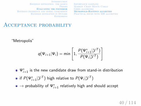
“Metropolis”
q(Ψi+1|Ψi ) = min
[1,
P(Ψ∗i+1|YT )
P(Ψi |YT )
]
Ψ∗i+1 is the new candidate draw from stand-in distribution
if P(Ψ∗i+1|YT ) high relative to P(Ψi |YT )
→ probability of Ψ∗i+1 relatively high and should accept
40 / 114
IntroductionBayesian estimation: the basics
PriorsEvaluating the posterior
Bayesian inference and model comparisonBayesian estimation in Dynare
Extensions
Importance samplingMarkov Chain Monte CarloGibbs algorithmMetropolis-Hastings algorithmPractical issues with MH algorithm
Acceptance probability
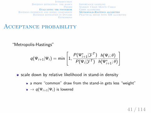
“Metropolis-Hastings”
q(Ψi+1|Ψi ) = min
[1,
P(Ψ∗i+1|YT )
P(Ψi |YT )
h(Ψi ; θ)
h(Ψ∗i+1; θ)
]
scale down by relative likelihood in stand-in density
a more “common” draw from the stand-in gets less “weight”
→ q(Ψi+1|Ψi ) is lowered
41 / 114
IntroductionBayesian estimation: the basics
PriorsEvaluating the posterior
Bayesian inference and model comparisonBayesian estimation in Dynare
Extensions
Importance samplingMarkov Chain Monte CarloGibbs algorithmMetropolis-Hastings algorithmPractical issues with MH algorithm
Acceptance probability
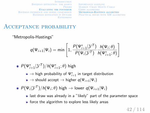
“Metropolis-Hastings”
q(Ψi+1|Ψi ) = min
[1,
P(Ψ∗i+1|YT )
P(Ψi |YT )
h(Ψi ; θ)
h(Ψ∗i+1; θ)
]
P(Ψ∗i+1|YT )/h(Ψ∗i+1; θ) high
→ high probability of Ψ∗i+1 in target distribution
→ should accept → higher q(Ψi+1|Ψi )
P(Ψi |YT )/h(Ψi ; θ) high → lower q(Ψi+1|Ψi )
last draw was already in a ”likely” part of the parameter space
force the algorithm to explore less likely areas
42 / 114
IntroductionBayesian estimation: the basics
PriorsEvaluating the posterior
Bayesian inference and model comparisonBayesian estimation in Dynare
Extensions
Importance samplingMarkov Chain Monte CarloGibbs algorithmMetropolis-Hastings algorithmPractical issues with MH algorithm
Updating the stand-in density
“Independence chain variant”
stand-in distribution does not change
it is independent across Monte Carlo replications
this is also the case in importance-sampling
43 / 114
IntroductionBayesian estimation: the basics
PriorsEvaluating the posterior
Bayesian inference and model comparisonBayesian estimation in Dynare
Extensions
Importance samplingMarkov Chain Monte CarloGibbs algorithmMetropolis-Hastings algorithmPractical issues with MH algorithm
Updating the stand-in density
“Random walk variant”
candidate draws are obtained according to Ψ∗i+1 = Ψi + εi+1
εi from a symmetric density around 0 and variance σ2h
as if the mean of the stand-in density adjusts with eachaccepted draw
in θ, µh = Ψi
44 / 114

IntroductionBayesian estimation: the basics
PriorsEvaluating the posterior
Bayesian inference and model comparisonBayesian estimation in Dynare
Extensions
Importance samplingMarkov Chain Monte CarloGibbs algorithmMetropolis-Hastings algorithmPractical issues with MH algorithm
Summary of MCMC with MH algorithm
1. maximize log-posterior logP(YT |Ψ) + logP(Ψ)
this yields the posterior mode Ψ
2. draw from a stand-in distribution h(Ψ; θ)
should have fatter tails than posterior
3. accept/reject based on probability q(Ψi+1|Ψi )
Metropolis vs. Metropolis-Hastings specification
4. go back to 2
adjust (random walk variant) stand-in distribution
do not adjust (independence variant) stand-in distribution
45 / 114

IntroductionBayesian estimation: the basics
PriorsEvaluating the posterior
Bayesian inference and model comparisonBayesian estimation in Dynare
Extensions
Importance samplingMarkov Chain Monte CarloGibbs algorithmMetropolis-Hastings algorithmPractical issues with MH algorithm
Summary of MCMC with MH algorithm
evaluation of the likelihood (step 1 and 3) requires
computation of the steady state
solution of the model
constructing the likelihood function (via the Kalman filter)
46 / 114
IntroductionBayesian estimation: the basics
PriorsEvaluating the posterior
Bayesian inference and model comparisonBayesian estimation in Dynare
Extensions
Importance samplingMarkov Chain Monte CarloGibbs algorithmMetropolis-Hastings algorithmPractical issues with MH algorithm
Choice of stand-in density
stand-in should have fatter tails
variance parameter important for acceptance rate
optimal acceptance rates:
around 0.44 for estimation of 1 parameter
around 0.23 for estimation of more than 5 parameters
47 / 114

IntroductionBayesian estimation: the basics
PriorsEvaluating the posterior
Bayesian inference and model comparisonBayesian estimation in Dynare
Extensions
Importance samplingMarkov Chain Monte CarloGibbs algorithmMetropolis-Hastings algorithmPractical issues with MH algorithm
Choice of stand-in density
often, stand-in is N(Ψ, c2ΣΨ)
Ψ is the posterior mode
ΣΨ is the inverse (negative) Hessian at the mode
tip: start with c = 2.4/√d
d is number of estimated parameters
increase (decrease) c if acceptance rate is too high (low)
48 / 114
IntroductionBayesian estimation: the basics
PriorsEvaluating the posterior
Bayesian inference and model comparisonBayesian estimation in Dynare
Extensions
Importance samplingMarkov Chain Monte CarloGibbs algorithmMetropolis-Hastings algorithmPractical issues with MH algorithm
Convergence statistics
theory says that distribution will converge to target
when does this happen?
→ diagnostic tests
sequence of draws should be from the invariant distribution
moments should not change within/between sequences
49 / 114
IntroductionBayesian estimation: the basics
PriorsEvaluating the posterior
Bayesian inference and model comparisonBayesian estimation in Dynare
Extensions
Importance samplingMarkov Chain Monte CarloGibbs algorithmMetropolis-Hastings algorithmPractical issues with MH algorithm
Brooks and Gelman statistics
I draws and J sequences
W =1
J
J∑j=1
1
I − 1
I∑i=1
(Ψi ,j −Ψj
)2
B =I
J
J∑j=1
(Ψj −Ψ
)2
B/I : estimate of the variance of the mean across sequences
W : estimate of average variance within sequences
50 / 114
IntroductionBayesian estimation: the basics
PriorsEvaluating the posterior
Bayesian inference and model comparisonBayesian estimation in Dynare
Extensions
Importance samplingMarkov Chain Monte CarloGibbs algorithmMetropolis-Hastings algorithmPractical issues with MH algorithm
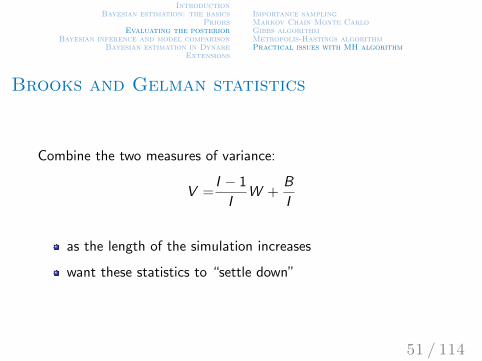
Brooks and Gelman statistics
Combine the two measures of variance:
V =I − 1
IW +
B
I
as the length of the simulation increases
want these statistics to “settle down”
51 / 114
IntroductionBayesian estimation: the basics
PriorsEvaluating the posterior
Bayesian inference and model comparisonBayesian estimation in Dynare
Extensions
Importance samplingMarkov Chain Monte CarloGibbs algorithmMetropolis-Hastings algorithmPractical issues with MH algorithm
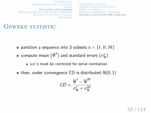
Geweke statistic
partition a sequence into 3 subsets s = I , II , III
compute mean (Ψs) and standard errors (σs
Ψ)
s.e.’s must be corrected for serial correlation
then, under convergence CD is distributed N(0, 1)
CD =Ψ
I −ΨIII
σIΨ + σIII
Ψ
52 / 114
IntroductionBayesian estimation: the basics
PriorsEvaluating the posterior
Bayesian inference and model comparisonBayesian estimation in Dynare
Extensions
Bayesian vs. frequentist inferenceHighest posterior density intervalsBayes factorsModel comparison
Bayesian inference and model comparison
53 / 114
IntroductionBayesian estimation: the basics
PriorsEvaluating the posterior
Bayesian inference and model comparisonBayesian estimation in Dynare
Extensions
Bayesian vs. frequentist inferenceHighest posterior density intervalsBayes factorsModel comparison
Bayesian vs. frequentist inference
Bayesian inference cannot use frequentist principles
t-test, F-test, LR-test etc.
they have a frequentist justification of repeated sampling
instead, there are two common Bayesian principles:
Highest Posterior Density (HPD) interval
Bayes factors (posterior odds)
54 / 114
IntroductionBayesian estimation: the basics
PriorsEvaluating the posterior
Bayesian inference and model comparisonBayesian estimation in Dynare
Extensions
Bayesian vs. frequentist inferenceHighest posterior density intervalsBayes factorsModel comparison
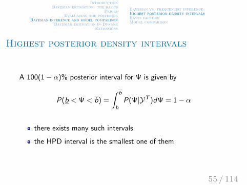
Highest posterior density intervals
A 100(1− α)% posterior interval for Ψ is given by
P(b < Ψ < b) =
∫ b
bP(Ψ|YT )dΨ = 1− α
there exists many such intervals
the HPD interval is the smallest one of them
55 / 114
IntroductionBayesian estimation: the basics
PriorsEvaluating the posterior
Bayesian inference and model comparisonBayesian estimation in Dynare
Extensions
Bayesian vs. frequentist inferenceHighest posterior density intervalsBayes factorsModel comparison
HPD “tests”
the HPD test amounts to checking whether Ψi ∈ HPD1−α
this is an informal way of comparing nested models
i.e. different parameter values
Bayesians can also compare non-nested models
56 / 114
IntroductionBayesian estimation: the basics
PriorsEvaluating the posterior
Bayesian inference and model comparisonBayesian estimation in Dynare
Extensions
Bayesian vs. frequentist inferenceHighest posterior density intervalsBayes factorsModel comparison
Bayes factors
B =P(YT |Ψ1)P(Ψ1)
P(YT |Ψ2)P(Ψ2)
where Ψ1 and Ψ2 are two different sets of parameter values
if B > 1 → Ψ1 is a posteriori more likely than Ψ2
57 / 114
IntroductionBayesian estimation: the basics
PriorsEvaluating the posterior
Bayesian inference and model comparisonBayesian estimation in Dynare
Extensions
Bayesian vs. frequentist inferenceHighest posterior density intervalsBayes factorsModel comparison
Model comparison
posterior densities can be used to evaluate
conditional probabilities of particular parameter values
conditional probabilities of different model specifications
use Bayes factors (posterior odds ratio) to compare models
advantage is that all models are treated symmetrically
there is no “null” model compared to an alternative
58 / 114
IntroductionBayesian estimation: the basics
PriorsEvaluating the posterior
Bayesian inference and model comparisonBayesian estimation in Dynare
Extensions
Bayesian vs. frequentist inferenceHighest posterior density intervalsBayes factorsModel comparison
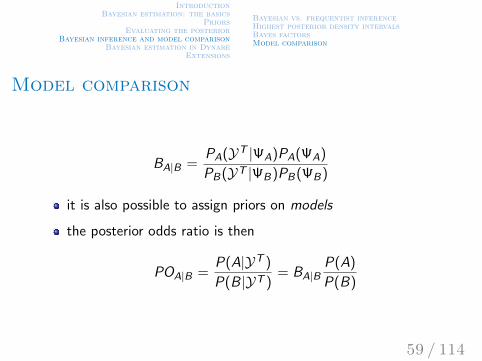
Model comparison
BA|B =PA(YT |ΨA)PA(ΨA)
PB(YT |ΨB)PB(ΨB)
it is also possible to assign priors on models
the posterior odds ratio is then
POA|B =P(A|YT )
P(B|YT )= BA|B
P(A)
P(B)
59 / 114
IntroductionBayesian estimation: the basics
PriorsEvaluating the posterior
Bayesian inference and model comparisonBayesian estimation in Dynare
Extensions
Bayesian vs. frequentist inferenceHighest posterior density intervalsBayes factorsModel comparison
Model comparison
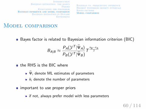
Bayes factor is related to Bayesian information criterion (BIC)
BA|B ≈PA(YT |ΨA)
PB(YT |ΨB)T
kB−kA2
the RHS is the BIC where
Ψi denote ML estimates of parameters
ki denote the number of parameters
important to use proper priors
if not, always prefer model with less parameters
60 / 114
IntroductionBayesian estimation: the basics
PriorsEvaluating the posterior
Bayesian inference and model comparisonBayesian estimation in Dynare
Extensions
Bayesian vs. frequentist inferenceHighest posterior density intervalsBayes factorsModel comparison
How much information in Bayes factor?
Kass and Raftery (1995), if the value of BA|B is
between 1 and 3 → barely worth mentioning
between 3 and 20 → positive evidence
between 20 and 150 → strong evidence
over 150 → very strong evidence
61 / 114
IntroductionBayesian estimation: the basics
PriorsEvaluating the posterior
Bayesian inference and model comparisonBayesian estimation in Dynare
Extensions
PreliminariesPriors and steady stateEstimation commandDecompositionOutputExample
Bayesian estimation in Dynare
62 / 114
IntroductionBayesian estimation: the basics
PriorsEvaluating the posterior
Bayesian inference and model comparisonBayesian estimation in Dynare
Extensions
PreliminariesPriors and steady stateEstimation commandDecompositionOutputExample
Preliminaries
setup is the same as with ML estimation
always a good idea to solve model first
some parameter values are likely to remain calibrated
63 / 114
IntroductionBayesian estimation: the basics
PriorsEvaluating the posterior
Bayesian inference and model comparisonBayesian estimation in Dynare
Extensions
PreliminariesPriors and steady stateEstimation commandDecompositionOutputExample
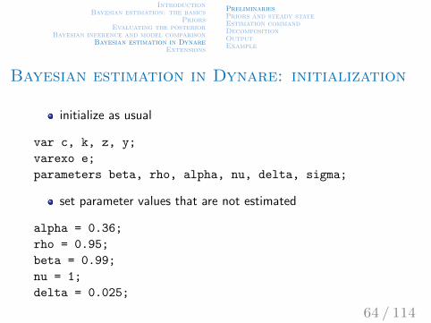
Bayesian estimation in Dynare: initialization
initialize as usual
var c, k, z, y;
varexo e;
parameters beta, rho, alpha, nu, delta, sigma;
set parameter values that are not estimated
alpha = 0.36;
rho = 0.95;
beta = 0.99;
nu = 1;
delta = 0.025;
64 / 114
IntroductionBayesian estimation: the basics
PriorsEvaluating the posterior
Bayesian inference and model comparisonBayesian estimation in Dynare
Extensions
PreliminariesPriors and steady stateEstimation commandDecompositionOutputExample
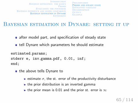
Bayesian estimation in Dynare: setting it up
after model part, and specification of steady state
tell Dynare which parameters he should estimate
estimated params;
stderr e, inv gamma pdf, 0.01, inf;
end;
the above tells Dynare to
estimate σ, the st. error of the productivity disturbance
the prior distribution is an inverted gamma
the prior mean is 0.01 and the prior st. error is ∞
65 / 114
IntroductionBayesian estimation: the basics
PriorsEvaluating the posterior
Bayesian inference and model comparisonBayesian estimation in Dynare
Extensions
PreliminariesPriors and steady stateEstimation commandDecompositionOutputExample
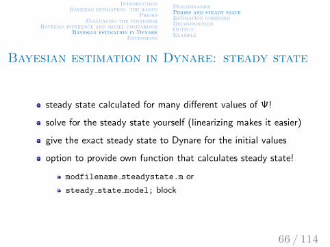
Bayesian estimation in Dynare: steady state
steady state calculated for many different values of Ψ!
solve for the steady state yourself (linearizing makes it easier)
give the exact steady state to Dynare for the initial values
option to provide own function that calculates steady state!
modfilename steadystate.m or
steady state model; block
66 / 114
IntroductionBayesian estimation: the basics
PriorsEvaluating the posterior
Bayesian inference and model comparisonBayesian estimation in Dynare
Extensions
PreliminariesPriors and steady stateEstimation commandDecompositionOutputExample
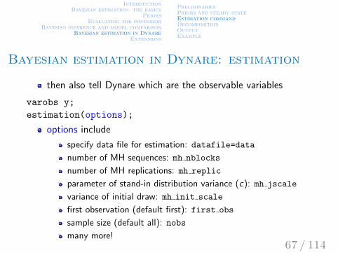
Bayesian estimation in Dynare: estimation
then also tell Dynare which are the observable variables
varobs y;
estimation(options);
options include
specify data file for estimation: datafile=data
number of MH sequences: mh nblocks
number of MH replications: mh replic
parameter of stand-in distribution variance (c): mh jscale
variance of initial draw: mh init scale
first observation (default first): first obs
sample size (default all): nobs
many more!67 / 114
IntroductionBayesian estimation: the basics
PriorsEvaluating the posterior
Bayesian inference and model comparisonBayesian estimation in Dynare
Extensions
PreliminariesPriors and steady stateEstimation commandDecompositionOutputExample
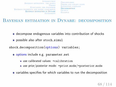
Bayesian estimation in Dynare: decomposition
decompose endogenous variables into contribution of shocks
possible also after stoch simul
shock decomposition(options) variables;
options include e.g. parameter set
use calibrated values: =calibration
use prior/posterior mode: =prior mode/=posterior mode
variables specifies for which variables to run the decomposition
68 / 114
IntroductionBayesian estimation: the basics
PriorsEvaluating the posterior
Bayesian inference and model comparisonBayesian estimation in Dynare
Extensions
PreliminariesPriors and steady stateEstimation commandDecompositionOutputExample
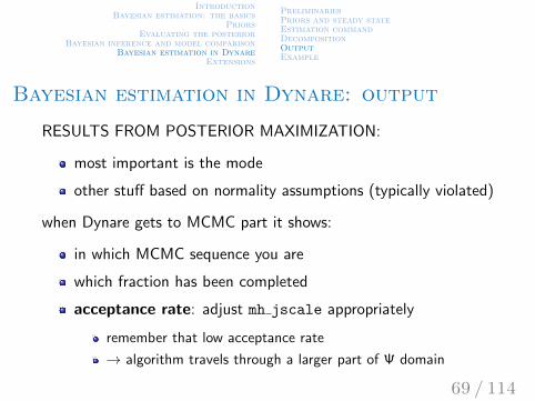
Bayesian estimation in Dynare: output
RESULTS FROM POSTERIOR MAXIMIZATION:
most important is the mode
other stuff based on normality assumptions (typically violated)
when Dynare gets to MCMC part it shows:
in which MCMC sequence you are
which fraction has been completed
acceptance rate: adjust mh jscale appropriately
remember that low acceptance rate
→ algorithm travels through a larger part of Ψ domain
69 / 114

IntroductionBayesian estimation: the basics
PriorsEvaluating the posterior
Bayesian inference and model comparisonBayesian estimation in Dynare
Extensions
PreliminariesPriors and steady stateEstimation commandDecompositionOutputExample
Bayesian estimation in Dynare: plots
priors
MCMC diagnostics
prior and posterior densities
shocks implied at the mode
observables and corresponding implied values
70 / 114
IntroductionBayesian estimation: the basics
PriorsEvaluating the posterior
Bayesian inference and model comparisonBayesian estimation in Dynare
Extensions
PreliminariesPriors and steady stateEstimation commandDecompositionOutputExample
Estimating the neoclassical growth model
use neoclassical growth model as data generating process
265 observations of output
use Bayesian estimation to estimate
σ
σ, ρ, δ, α
71 / 114
IntroductionBayesian estimation: the basics
PriorsEvaluating the posterior
Bayesian inference and model comparisonBayesian estimation in Dynare
Extensions
PreliminariesPriors and steady stateEstimation commandDecompositionOutputExample
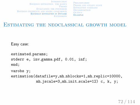
Estimating the neoclassical growth model
Easy case:
estimated params;
stderr e, inv gamma pdf, 0.01, inf;
end;
varobs y;
estimation(datafile=y,mh nblocks=1,mh replic=10000,
mh jscale=3,mh init scale=12) c, k, y;
72 / 114
IntroductionBayesian estimation: the basics
PriorsEvaluating the posterior
Bayesian inference and model comparisonBayesian estimation in Dynare
Extensions
PreliminariesPriors and steady stateEstimation commandDecompositionOutputExample
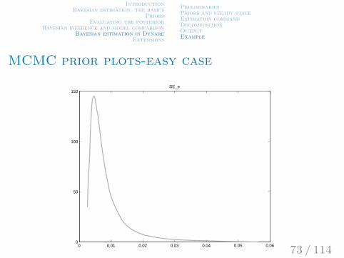
MCMC prior plots-easy case
0 0.01 0.02 0.03 0.04 0.05 0.060
50
100
150SE_e
73 / 114
IntroductionBayesian estimation: the basics
PriorsEvaluating the posterior
Bayesian inference and model comparisonBayesian estimation in Dynare
Extensions
PreliminariesPriors and steady stateEstimation commandDecompositionOutputExample
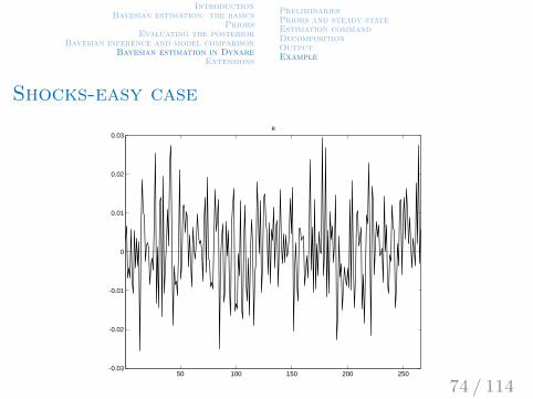
Shocks-easy case
50 100 150 200 250-0.03
-0.02
-0.01
0
0.01
0.02
0.03e
74 / 114
IntroductionBayesian estimation: the basics
PriorsEvaluating the posterior
Bayesian inference and model comparisonBayesian estimation in Dynare
Extensions
PreliminariesPriors and steady stateEstimation commandDecompositionOutputExample
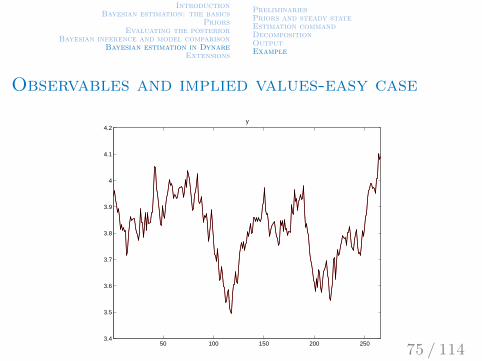
Observables and implied values-easy case
50 100 150 200 2503.4
3.5
3.6
3.7
3.8
3.9
4
4.1
4.2y
75 / 114
IntroductionBayesian estimation: the basics
PriorsEvaluating the posterior
Bayesian inference and model comparisonBayesian estimation in Dynare
Extensions
PreliminariesPriors and steady stateEstimation commandDecompositionOutputExample
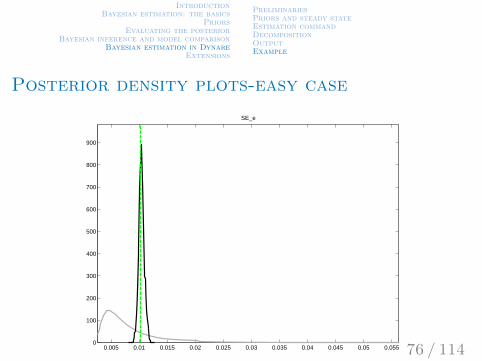
Posterior density plots-easy case
0.005 0.01 0.015 0.02 0.025 0.03 0.035 0.04 0.045 0.05 0.0550
100
200
300
400
500
600
700
800
900
SE_e
76 / 114

IntroductionBayesian estimation: the basics
PriorsEvaluating the posterior
Bayesian inference and model comparisonBayesian estimation in Dynare
Extensions
PreliminariesPriors and steady stateEstimation commandDecompositionOutputExample
Printed results - easy case
Posterior mode:
0.0103 (0.0004)
Average acceptance rate:
37.7%
Diagnostic statistics (Geweke):p-values on equality of means in sub-samples
0.037 (no taper) 0.33 (4% taper) 0.38 (8% taper) etc.
Posterior mean and HPD interval:
0.0104 (0.0096 - 0.0111)
77 / 114
IntroductionBayesian estimation: the basics
PriorsEvaluating the posterior
Bayesian inference and model comparisonBayesian estimation in Dynare
Extensions
PreliminariesPriors and steady stateEstimation commandDecompositionOutputExample
What we did today
Basic concept of Bayesian estimation
priors
evaluating the posterior
Markov Chain Monte Carlo (MCMC)
practical issues
acceptance rate, diagnostics
implementation in Dynare
78 / 114
IntroductionBayesian estimation: the basics
PriorsEvaluating the posterior
Bayesian inference and model comparisonBayesian estimation in Dynare
Extensions
PreliminariesPriors and steady stateEstimation commandDecompositionOutputExample
What we did in the first half of course
Motivation
Week 1: Use of computational tools, simple DSGE model X
Tools necessary to solve models and a solution method
Week 2: function approximation and numerical integration X
Week 3: theory of perturbation (1st and higher-order) X
Tools necessary for, and principles of, estimation
Week 4: Kalman filter and Maximum Likelihood estimation X
Week 5: principles of Bayesian estimation X
79 / 114
IntroductionBayesian estimation: the basics
PriorsEvaluating the posterior
Bayesian inference and model comparisonBayesian estimation in Dynare
Extensions
PreliminariesPriors and steady stateEstimation commandDecompositionOutputExample
Extensions
80 / 114

IntroductionBayesian estimation: the basics
PriorsEvaluating the posterior
Bayesian inference and model comparisonBayesian estimation in Dynare
Extensions
TrendsMore on priorsAlternatives
Trends
Problem:
methodology works for stationary environments
data has trends
not clear which trend the model represents?
81 / 114

IntroductionBayesian estimation: the basics
PriorsEvaluating the posterior
Bayesian inference and model comparisonBayesian estimation in Dynare
Extensions
TrendsMore on priorsAlternatives
Trends
1940 1950 1960 1970 1980 1990 2000 2010 2020-15
-10
-5
0
5
10
devi
atio
ns fr
om tr
end
(%)
HP (1600)
HP(105)
linear
quadratic
BP(6,32)
82 / 114
IntroductionBayesian estimation: the basics
PriorsEvaluating the posterior
Bayesian inference and model comparisonBayesian estimation in Dynare
Extensions
TrendsMore on priorsAlternatives
Trends
we could build in a trend within the model
e.g. productivity is trending
“stationarize” non-stationary variables within the model
i.e. inspect variables relative to productivity
however, not clear that data satisfies balanced growth
83 / 114
IntroductionBayesian estimation: the basics
PriorsEvaluating the posterior
Bayesian inference and model comparisonBayesian estimation in Dynare
Extensions
TrendsMore on priorsAlternatives
Trends
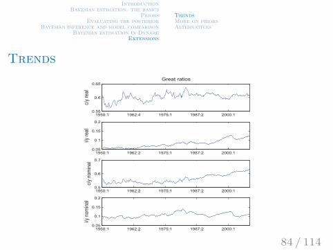
b) Build-in a trend into the model. Detrend the data with model-based-trend. Problem: data does not seem to satisfy balanced growth.
1950:1 1962:4 1975:1 1987:2 2000:10.55
0.6
0.65Great ratios
c/y re
al
1950:1 1962:2 1975:1 1987:2 2000:10.05
0.1
0.15
0.2
i/y re
al
1950:1 1962:2 1975:1 1987:2 2000:10.5
0.6
0.7
c/y n
omina
l
1950:1 1962:2 1975:1 1987:2 2000:10.05
0.1
0.15
0.2
i/y n
omina
l
0 0.2 0.4 0.6 0.8 1−20
−10
0Log spectra
0 0.2 0.4 0.6 0.8 1−20
−10
0
0 0.2 0.4 0.6 0.8 1−20
−10
0
0 0.2 0.4 0.6 0.8 1−20
−10
0
Real and nominal Great ratios in US, 1950-2008.
84 / 114
IntroductionBayesian estimation: the basics
PriorsEvaluating the posterior
Bayesian inference and model comparisonBayesian estimation in Dynare
Extensions
TrendsMore on priorsAlternatives
Trends
Solutions:
use differenced data
highlights high-frequency movements (measurement error)
detrend prior to estimation
85 / 114
IntroductionBayesian estimation: the basics
PriorsEvaluating the posterior
Bayesian inference and model comparisonBayesian estimation in Dynare
Extensions
TrendsMore on priorsAlternatives
Estimation on detrended data
use e.g. quadratic trend:
yt = a0 + a1t + a2t2 + ut
each variable can have its own trend
using HP or Band Pass filter:
yobs−filteredt = B(L)yobs
t
B(L) is a 2-sided filter!
→ creates artificial serial correlation in the filtered data
→ apply filter also to model data
86 / 114
IntroductionBayesian estimation: the basics
PriorsEvaluating the posterior
Bayesian inference and model comparisonBayesian estimation in Dynare
Extensions
TrendsMore on priorsAlternatives
Estimation on detrended data
the above implies that the model is fitted to low(er)frequencies only
Canova (2010) points out that the above can lead to:
underestimated volatility of shocks
persistence of shocks is overestimated
less perceived noise → decisions rules imply higherpredictability
substitution and income effects may be distorted due to theabove
proposes to estimate flexible trend specifications within model
87 / 114
IntroductionBayesian estimation: the basics
PriorsEvaluating the posterior
Bayesian inference and model comparisonBayesian estimation in Dynare
Extensions
TrendsMore on priorsAlternatives
More on selecting priors
what we’ve described is based on selecting (independent)priors about deep parameters
however, often we have priors about observables
moreover, reasonable independent priors may form ratherunreasonable properties of the model
solutions proposed in the literature:
Del Negro, Schorfheide (2008)
Andrle, Benes (2013)
Jarocinsky, Marcet (2013)
88 / 114
IntroductionBayesian estimation: the basics
PriorsEvaluating the posterior
Bayesian inference and model comparisonBayesian estimation in Dynare
Extensions
TrendsMore on priorsAlternatives
Del Negro, Schorfheide (2008)
more guidance for eliciting priors
three main issues with (independent) priors about deepparameters:
may lead to probability mass on unrealistic properties of themodel
most exogenous shock processes are latent, i.e. difficult toform priors about
priors are often transfered to different models
89 / 114

IntroductionBayesian estimation: the basics
PriorsEvaluating the posterior
Bayesian inference and model comparisonBayesian estimation in Dynare
Extensions
TrendsMore on priorsAlternatives
Del Negro, Schorfheide (2008)
they group parameters into three categories:
those determining the steady state
those determining exogenous shocks
those determining the endogenous propagation mechanism
90 / 114

IntroductionBayesian estimation: the basics
PriorsEvaluating the posterior
Bayesian inference and model comparisonBayesian estimation in Dynare
Extensions
TrendsMore on priorsAlternatives
Del Negro, Schorfheide (2008)
Parameters related to steady state relationships
discount rate, depreciation, returns to scale, inflation targetetc.
let SD(Ψss) be a vector of steady state relationshipsdepending on a set of parameters Ψss
then S = SD(Ψss) + η are measurements of thoserelationships with measurement error η
S has a probabilistic interpretation and therefore
using Bayes’ rule, one can write P(Ψss |S) ∝ L(S |Ψss)P(Ψss)
allows for overidentification
91 / 114
IntroductionBayesian estimation: the basics
PriorsEvaluating the posterior
Bayesian inference and model comparisonBayesian estimation in Dynare
Extensions
TrendsMore on priorsAlternatives
Del Negro, Schorfheide (2008)
Exogenous processes
volatility and persistence parameters
use implied moments of endogenous variables to “back out”priors
the above is given values for Ψss and Ψendo
→ valid for a particular model and should not be directlytransfered across models
92 / 114

IntroductionBayesian estimation: the basics
PriorsEvaluating the posterior
Bayesian inference and model comparisonBayesian estimation in Dynare
Extensions
TrendsMore on priorsAlternatives
Del Negro, Schorfheide (2008)
Endogenous propagation mechanisms
price rigidity, labor supply elasticity etc.
one could use similar principle as above
authors suggest independent priors because researchers oftenhave a relatively good idea
note that the joint prior induces non-trivial non-linearrelationships between parameters
joint prior becomes
P(Ψ|S) ∝ L(S |Ψss)P(Ψss)P(Ψendo)
requires an additional step in MCMC algorithm
93 / 114
IntroductionBayesian estimation: the basics
PriorsEvaluating the posterior
Bayesian inference and model comparisonBayesian estimation in Dynare
Extensions
TrendsMore on priorsAlternatives
Andrle, Benes (2013)
Andrle and Benes do not distinguish between groups ofparameters
their “system priors” are priors about concepts such as
impulse response functions
conditional correlations etc.
94 / 114
IntroductionBayesian estimation: the basics
PriorsEvaluating the posterior
Bayesian inference and model comparisonBayesian estimation in Dynare
Extensions
TrendsMore on priorsAlternatives
Andrle, Benes (2013)
even sensible individual-parameter priors can lead tounintended properties of the aggregate model
independence of priors can lead to substantial mass on suchparameter regions
call for careful prior-predictive analysis:
IRFs, second moments ...
compare with posterior results
is it the data or the model driving the results?
95 / 114
IntroductionBayesian estimation: the basics
PriorsEvaluating the posterior
Bayesian inference and model comparisonBayesian estimation in Dynare
Extensions
TrendsMore on priorsAlternatives
Andrle, Benes (2013)
Candidates for system priors:
steady states
sensible values in levels or growth rates
(un-)conditional moments
cross-correlations (conditional on shocks)
impulse response properties
peak impacts, duration, horizon of monetary policyeffectiveness etc.
96 / 114
IntroductionBayesian estimation: the basics
PriorsEvaluating the posterior
Bayesian inference and model comparisonBayesian estimation in Dynare
Extensions
TrendsMore on priorsAlternatives
Andrle, Benes (2013)
Implementation:
use Bayes’ rule again
specify model properties you care about Z = h(Ψ)
these can be characterized by a probabilistic modelZ ∼ D(Z s)
D(Z s) is a distribution function
Z s are parameters of that function (hyper-parameters)
its likelihood function (the system prior): P(Z s |Ψ, h)
composite joint prior: P(Ψ|Z s , h) ∝ P(Z s |Ψ, h)P(Ψ)
97 / 114
IntroductionBayesian estimation: the basics
PriorsEvaluating the posterior
Bayesian inference and model comparisonBayesian estimation in Dynare
Extensions
TrendsMore on priorsAlternatives
Andrle, Benes (2013)
The posterior becomes
P(Ψ|YT ,Z s) ∝ L(YT |Ψ)P(Z s |Ψ, h)P(Ψ)
evaluation is in principle the same as before
use of MCMC methods
additional step in evaluating the system prior
slows things down - have to run MCMC on prior (withlikelihood “switched off”) and then posterior
98 / 114

IntroductionBayesian estimation: the basics
PriorsEvaluating the posterior
Bayesian inference and model comparisonBayesian estimation in Dynare
Extensions
TrendsMore on priorsAlternatives
Jarocinsky, Marcet (2013)
similar ideas as above, but in the context of Bayesian VARs
their point is that widely used priors about parameters
can lead to behavior of observables that is counterfactual
→ always a good to do prior-predictive analysis of you model!
99 / 114
IntroductionBayesian estimation: the basics
PriorsEvaluating the posterior
Bayesian inference and model comparisonBayesian estimation in Dynare
Extensions
TrendsMore on priorsAlternatives
Alternatives to Bayesian estimation
Maximum likelihood
calibration
GMM
SMM & indirect inference
100 / 114

IntroductionBayesian estimation: the basics
PriorsEvaluating the posterior
Bayesian inference and model comparisonBayesian estimation in Dynare
Extensions
TrendsMore on priorsAlternatives
Maximum likelihood
we’ve seen it yesterday
conceptually different from Bayesian estimation
tools required part of Bayesian estimation
101 / 114

IntroductionBayesian estimation: the basics
PriorsEvaluating the posterior
Bayesian inference and model comparisonBayesian estimation in Dynare
Extensions
TrendsMore on priorsAlternatives
Calibration
wide-spread methodology at least since Kydland and Prescott(1982)
prior to this, state-of-the-art were systems of simultaneousequations
those were viewed as “true statistical” models to be estimated
102 / 114
IntroductionBayesian estimation: the basics
PriorsEvaluating the posterior
Bayesian inference and model comparisonBayesian estimation in Dynare
Extensions
TrendsMore on priorsAlternatives
Calibration
although calibration is also an empirical exercise
it lacks the probabilistic interpretation
the constraint is that the model mimics (a priori identified)features in the data
Kydland and Prescott (1996):It is important to emphasize that the parameter values selected arenot the ones that provide the best fit in some statistical sense.
103 / 114
IntroductionBayesian estimation: the basics
PriorsEvaluating the posterior
Bayesian inference and model comparisonBayesian estimation in Dynare
Extensions
TrendsMore on priorsAlternatives
Calibration
Parameters are pinned down by a selection of real-world features
long-run averages (labor share, hours worked)
micro studies (preference parameters)
certain business cycle properties of the data (shockparameters) etc.
104 / 114

IntroductionBayesian estimation: the basics
PriorsEvaluating the posterior
Bayesian inference and model comparisonBayesian estimation in Dynare
Extensions
TrendsMore on priorsAlternatives
Calibration
compare different features of the data to model predictions
closely related to moment-matching (estimating models)
however, calibration lacks the statistical formality
the above is a strong source of criticism of calibration
no formal rules on selecting dimension to which model is fit
no formal rules of comparing alternatives - models arenecessarily misspecified
not that the last point does not hold for Bayesian modelcomparison
105 / 114
IntroductionBayesian estimation: the basics
PriorsEvaluating the posterior
Bayesian inference and model comparisonBayesian estimation in Dynare
Extensions
TrendsMore on priorsAlternatives
Matching moments (GMM, SMM, II)
idea similar to calibration:
a set of moments (features) of the data used to parameterizemodel
a different set of moments used to judge the performance ofmodel
matching moments adds statistical rigor
estimation
hypothesis testing
106 / 114
IntroductionBayesian estimation: the basics
PriorsEvaluating the posterior
Bayesian inference and model comparisonBayesian estimation in Dynare
Extensions
TrendsMore on priorsAlternatives
Matching moments (GMM, SMM, II)
as with calibration, moment matching is based on a selectionof moments
often referred to as limited-information procedures
a full range of statistical implications contained in model’slikelihood function
disadvantages of limited-information procedures
potential loss of efficiency
inference potentially sensitive to selected moments
advantages of limited-information procedures
no need to make distributional assumptions
107 / 114
IntroductionBayesian estimation: the basics
PriorsEvaluating the posterior
Bayesian inference and model comparisonBayesian estimation in Dynare
Extensions
TrendsMore on priorsAlternatives
Generalized method of moments
attributed to Hansen (1982), generalization, asymptoticproperties
the main idea is to use “orthogonality conditions” (e.g.first-order-conditions)
E[f (xt ,Ψ)] = 0
xt is a vector of variables
Ψ are model parameters
108 / 114
IntroductionBayesian estimation: the basics
PriorsEvaluating the posterior
Bayesian inference and model comparisonBayesian estimation in Dynare
Extensions
TrendsMore on priorsAlternatives
Generalized method of moments
pick Ψ s.t. the sample analogs of orthogonality conditionsg(X ,Ψ) = 1/T
∑t f (xt ,Ψ)
hold exactly, exactly identified case
number of parameters = number of moment conditions
are as close to zero as possible, overidentified case
are number of parameters < number of moment conditions
109 / 114

IntroductionBayesian estimation: the basics
PriorsEvaluating the posterior
Bayesian inference and model comparisonBayesian estimation in Dynare
Extensions
TrendsMore on priorsAlternatives
Generalized method of moments
in the over-identified case
minΨ
g(X ,Ψ)′Ωg(X ,Ψ)
Ω is a weighting matrix
the optimal weighting matrix is the inverse of the var-covarmatrix of g(X ,Ψ)
110 / 114
IntroductionBayesian estimation: the basics
PriorsEvaluating the posterior
Bayesian inference and model comparisonBayesian estimation in Dynare
Extensions
TrendsMore on priorsAlternatives
Simulated method of moments
in some cases the orthogonality conditions cannot be assessedanalytically
moment-matching estimation based on simulations retainsasymptotic properties of GMM
111 / 114
IntroductionBayesian estimation: the basics
PriorsEvaluating the posterior
Bayesian inference and model comparisonBayesian estimation in Dynare
Extensions
TrendsMore on priorsAlternatives
Simulated method of moments
let zt be model variables corresponding to data xt
let empirical targets be summarized by h(xt)
SMM estimation is based on
E[h(xt)] = E[h(zt ,Ψ)]
→ f (xt ,Ψ) = h(xt)− h(zt ,Ψ)
112 / 114
IntroductionBayesian estimation: the basics
PriorsEvaluating the posterior
Bayesian inference and model comparisonBayesian estimation in Dynare
Extensions
TrendsMore on priorsAlternatives
Indirect inference
based on reduced-form models
main idea is to use structural model to interpret reduced-formresults
can simulated data from a structural model replicate areduced-form estimate using real-world data?
i.e. it is a moment-matching exercise
moments are clearly defined by prior reduced-form analysis
113 / 114
IntroductionBayesian estimation: the basics
PriorsEvaluating the posterior
Bayesian inference and model comparisonBayesian estimation in Dynare
Extensions
TrendsMore on priorsAlternatives
Indirect inference
let δ be a vector of reduced-form estimates
δ(xt) are those in the data and δ(zt ,Ψ) are those from themodel
pick Ψ s.t.δ(xt) = δ(zt ,Ψ)
114 / 114