bayesian classifiers and probability estimation
TRANSCRIPT

Bayesian Classifiers and Probability Estimation
CSE 4308/5360: Artificial Intelligence I
University of Texas at Arlington
1

Data Space
• Suppose that we have a classification problem
• The patterns for this problem come from some underlying space X.
• Note that we use the term “space”.
• What is the difference between “space” and “set”?
– Not much. Oftentimes “space” and “set” refer to the same thing.
• However, note the distinction between these terms:
– Data space: the set of all possible patterns for a problem.
– Data set: a specific set of examples that we are given.
2

Types of Data Spaces
• The space X can be discrete or continuous.
• The space X can be finite or infinite.
• Examples of discrete and finite spaces?
3

Types of Data Spaces
• The space X can be discrete or continuous.
• The space X can be finite or infinite.
• Examples of discrete and finite spaces?
• The restaurant waiting problem.
• The satellite image dataset.
– Here, individual pixels of the image are classified.
– Each pixel is represented as a 36-dimensional vector.
– Each of the 36 values is an integer between 1 and 157.
4

Types of Data Spaces
• Examples of a discrete and infinite space?
5

Types of Data Spaces
• Examples of a discrete and infinite space?
• The set of videos.
– Each video is a sequence of images (frames).
– Each image is a sequence of pixels.
– Each pixel is a sequence of three integers, specifying the red, green, and blue component of the color.
– Each of these three RGB values is a number between 0 and 255.
• Assuming that a video may contain any number of frames, the number of possible videos is infinite.
6

Types of Data Spaces
• The space of images is an interesting case.
• Suppose that each image is a color image of size 100x100 pixels. – This is tiny compared to the size of typical photos today.
• Then, we have a finite number of possible images.
• What is that number?
7

Types of Data Spaces
• The space of images is an interesting case.
• Suppose that each image is a color image of size 100x100 pixels. – This is tiny compared to the size of typical photos today.
• Then, we have a finite number of possible images.
• What is that number?
• 25630,000 = 2240,000
• Why?
8

Types of Data Spaces
• The space of images is an interesting case.
• Suppose that each image is a color image of size 100x100 pixels. – This is tiny compared to the size of typical photos today.
• Then, we have a finite number of possible images.
• What is that number?
• 25630,000 = 2240,000
• Why? Because: – An image is defined by 30,000 numbers (10,000 pixels times 3 color
values).
– Each of those numbers has 256 possible values.
• So, technically the space of 100x100 images is discrete and finite, but practically you can treat it as discrete and infinite. 9
Types of Data Spaces
• Any examples of continuous and finite spaces?
10

Types of Data Spaces
• Any examples of continuous and finite spaces?
• No!
• If the space is finite, it means it can only have a finite number of elements.
• Finite number of elements means finite (and thus discrete) number of possible values.
11

Types of Data Spaces
• Any examples of continuous and infinite spaces?
12

Types of Data Spaces
• Any examples of continuous and infinite spaces?
• Any space where we represent data using continuous values.
• Examples of such continuous values:
– Weight.
– Height.
– Temperature.
– Distance.
• Example task: predict the gender of a chameleon based on its weight and length. 13

The Bayes Classifier
• Let X be the space of all possible patterns for some classification problem.
• Suppose that we have a function P(x | c) that produces the conditional probability of any x in X given any class label c.
• Suppose that we also know the prior probabilities P(c) of all classes c.
• Given this information, we can build the optimal (most accurate possible) classifier for our problem.
– We can prove that no other classifier can do better.
• This optimal classifier is called the Bayes classifier. 14

The Bayes Classifier
• So, how do we define this optimal classifier? Let's call it B.
• B(x) = ???
• Any ideas?
15

The Bayes Classifier
• First, for every class c, compute P(c | x) using Bayes rule.
• 𝑃 𝑐 𝑥) = 𝑃(𝑥 | 𝑐) ∗ 𝑃(𝑐)
𝑃(𝑥)
• To compute the above, we need to compute P(x). How can we compute P(x)?
• Let C be the set of all possible classes.
• 𝑃 𝑥 = 𝑃(𝑥 | 𝑐) ∗ 𝑃(𝑐)𝑐∈𝐶
16

The Bayes Classifier
𝑃 𝑐 𝑥) = 𝑃(𝑥 | 𝑐) ∗ 𝑃(𝑐)
𝑃(𝑥)
𝑃 𝑥 = 𝑃(𝑥 | 𝑐) ∗ 𝑃(𝑐)
𝑐∈𝐶
• Using 𝑃 𝑐 𝑥), we can now define the optimal classifier:
B x = ? ? ?
• Can anyone try to guess?
17

The Bayes Classifier
𝑃 𝑐 𝑥) = 𝑃(𝑥 | 𝑐) ∗ 𝑃(𝑐)
𝑃(𝑥)
𝑃 𝑥 = 𝑃(𝑥 | 𝑐) ∗ 𝑃(𝑐)
𝑐∈𝐶
• Using 𝑃 𝑐 𝑥), we can now define the optimal classifier:
B x = argmax𝑐∈𝐶𝑃(𝑐 | 𝑥)
• What does this mean? What is argmax𝑐∈𝐶𝑃(𝑐 | 𝑥)?
• It is the class c that maximizes P(c | x). 18

The Bayes Classifier
𝑃 𝑐 𝑥) = 𝑃(𝑥 | 𝑐) ∗ 𝑃(𝑐)
𝑃(𝑥)
𝑃 𝑥 = 𝑃(𝑥 | 𝑐) ∗ 𝑃(𝑐)
𝑐∈𝐶
• Using 𝑃 𝑐 𝑥), we can now define the optimal classifier:
B x = argmax𝑐∈𝐶𝑃(𝑐 | 𝑥)
• B(x) is called the Bayes Classifier.
• It is the most accurate classifier you can possibly get.
19

The Bayes Classifier
𝑃 𝑐 𝑥) = 𝑃(𝑥 | 𝑐) ∗ 𝑃(𝑐)
𝑃(𝑥)
𝑃 𝑥 = 𝑃(𝑥 | 𝑐) ∗ 𝑃(𝑐)
𝑐∈𝐶
• Using 𝑃 𝑐 𝑥), we can now define the optimal classifier:
B x = argmax𝑐∈𝐶𝑃(𝑐 | 𝑥)
• B(x) is called the Bayes Classifier.
• Important note: the above formulas can also be applied when P(x | c) is a probability density function.
20

Bayes Classifier Optimality
B x = argmax𝑐∈𝐶𝑃(𝑐 | 𝑥)
• Why is this a reasonable definition for B(x)?
• Why is it the best possible classifier?
• ???
21

Bayes Classifier Optimality
B x = argmax𝑐∈𝐶𝑃(𝑐 | 𝑥)
• Why is this a reasonable definition for B(x)?
• Why is it the best possible classifier?
• Because B(x) provides the answer that is most likely to be true.
• When we are not sure what the correct answer is, our best bet is the answer that is the most likely to be true.
22

Bayes Classifier Limitations
B x = argmax𝑐∈𝐶𝑃(𝑐 | 𝑥)
• Will such a classifier always have perfect accuracy?
23

Bayes Classifier Limitations
B x = argmax𝑐∈𝐶𝑃(𝑐 | 𝑥)
• Will such a classifier always have perfect accuracy?
• No. Here is a toy example:
• We want our classifier B(x) to predict whether a temperature x came from Maine or from the Sahara desert.
• Consider B(90). A temperature of 90 is possible in both places.
• Whatever B(90) returns, it will be wrong in some cases. – If B(90) = Sahara, then B will be wrong in the few cases where this 90 was
observed in Maine.
– If B(90) = Maine, then B will be wrong in the many cases where this 90 was observed in Sahara.
• The Bayesian classifier B returns for 90 the most likely answer (Sahara), so as to be correct as frequently as possible. 24

Bayes Classifier Limitations
B x = argmax𝑐∈𝐶𝑃(𝑐 | 𝑥)
• Actually (though this is a side issue), to be entirely accurate, there is a case where B(90) would return Maine, even though a temperature of 90 is much more common in Sahara.
• What is that case?
• The case where the prior probability for Sahara is really really low. – Sufficiently low to compensate for the fact that temperatures of 90 are
much more frequent there than in Maine.
• Remember, 𝑃 𝑆𝑎ℎ𝑎𝑟𝑎 𝑥) = 𝑃(𝑥 | 𝑆𝑎ℎ𝑎𝑟𝑎) ∗ 𝑃(𝑆𝑎ℎ𝑎𝑟𝑎)
𝑃(𝑥)
• If P(Sahara) is very low (if inputs x rarely come from Sahara), it drives P(Sahara | X) down as well.
25

Bayes Classifier Limitations
• So, we know the formula for the optimal classifier for any classification problem.
• Why don't we always use the Bayes classifier?
– Why are we going to study other classification methods in this class?
– Why are people still trying to come up with new classification methods, if we already know that none of them can beat the Bayes classifier?
26

Bayes Classifier Limitations
• So, we know the formula for the optimal classifier for any classification problem.
• Why don't we always use the Bayes classifier?
– Why are we going to study other classification methods in this class?
– Why are researchers still trying to come up with new classification methods, if we already know that none of them can beat the Bayes classifier?
• Because, sadly, the Bayes classifier has a catch.
– To construct the Bayes classifier, we need to compute P(x | c), for every x and every c.
– In most cases, we cannot compute P(x | c) precisely enough. 27

Problems with Estimating Probabilities
• To show why we usually cannot estimate probabilities precisely enough, we can consider again the example of the space of 100x100 images. – In that case, x is a vector of 30,000 dimensions.
• Suppose we want B(x) to predict whether x is a photograph of Michael Jordan or Kobe Bryant.
• P(x | Jordan) can be represented as a joint distribution table of 30,000 variables, one for each dimension. – Each variable has 256 possible values.
– We need to compute and store 25630,000 numbers.
• We have neither enough storage to store such a table, nor enough training data to compute all these values.
28

Options when Accurate Probabilities are Unknown
• In typical pattern classification problems, our data is too complex to allow us to compute probability distributions precisely.
• So, what can we do?
• ???
29

Options when Accurate Probabilities are Unknown
• In typical pattern classification problems, our data is too complex to allow us to compute probability distributions precisely.
• So, what can we do?
• We have two options.
• One is to not use a Bayes classifier.
• This is why other methods exist and are useful.
– An example: neural networks (we will see them in more detail in a few weeks).
– Other popular examples that we will not study: Boosting, support vector machines.
30

Options when Accurate Probabilities are Unknown
• The second option is to use a pseudo-Bayes classifier, and estimate approximate probabilities P(x | c).
• What is approximate?
– An approximate estimate is an estimate that is not expected to be 100% correct.
– An approximate method for estimating probabilities is a method that produces approximate estimates of probability distributions.
• Approximate methods are designed to require reasonable memory and reasonable amounts of training data, so that we can actually use them in practice.
31

Options when Accurate Probabilities are Unknown
• We will see several examples of such approximate methods, but you have already seen two approaches (and two associated programming assignments):
• ???
32

Options when Accurate Probabilities are Unknown
• We will see several examples of such approximate methods, but you have already seen two approaches (and two associated programming assignments):
• Bayesian networks is one approach for simplifying the representation of the joint probability distribution.
– Of course, Bayesian networks may be exact in some cases, but typically the variables have dependencies in the real world that the network topology ignores.
• Decision trees and random forests are another approach.
33

Decision Trees as Probability Estimates
• Why are decision trees and forests mentioned here as approximate methods for estimating probabilities?
34

Decision Trees as Probability Estimates
• Why are decision trees and forests mentioned here as approximate methods for estimating probabilities?
• In the assignment, what info do you store at each leaf?
35

Decision Trees as Probability Estimates
• Why are decision trees and forests mentioned here as approximate methods for estimating probabilities?
• In the assignment, what info do you store at each leaf?
– P(c | x)
• What is the output of a decision tree on some input x?
36

Decision Trees as Probability Estimates
• Why are decision trees and forests mentioned here as approximate methods for estimating probabilities?
• In the assignment, what info do you store at each leaf?
– P(c | x)
• What is the output of a decision tree on some input x?
• argmax𝑐∈𝐶𝑃(𝑐 | 𝑥), based on the P(c, x) stored on the leaf.
• What is the output of a decision forest on some input x?
37

Decision Trees as Probability Estimates
• Why are decision trees and forests mentioned here as approximate methods for estimating probabilities?
• In the assignment, what info do you store at each leaf?
– P(c | x)
• What is the output of a decision tree on some input x?
• argmax𝑐∈𝐶𝑃(𝑐 | 𝑥), based on the P(c, x) stored on the leaf.
• What is the output of a decision forest on some input x?
• argmax𝑐∈𝐶𝑃(𝑐 | 𝑥), based on the average of P(c | x) values
we get from each tree. 38

• The Bayesian classifier outputs argmax𝑐∈𝐶𝑃(𝑐 | 𝑥)
• Decision trees and forests also output argmax𝑐∈𝐶𝑃(𝑐 | 𝑥)
• So, are decision trees and forests Bayes classifiers? – Which would mean that no other classifier can do better!
39
Decision Trees as Probability Estimates

• The Bayesian classifier outputs argmax𝑐∈𝐶𝑃(𝑐 | 𝑥)
• Decision trees and forests also output argmax𝑐∈𝐶𝑃(𝑐 | 𝑥)
• So, are decision trees and forests Bayes classifiers? – Which would mean that no other classifier can do better!
• Theoretically, they are Bayes classifiers, in the (usually unrealistic) case that the probability distributions stored in the leaves are accurate.
• I call them “pseudo-Bayes” classifiers, because they look like Bayes classifiers, but use inaccurate probabilities.
40
Decision Trees as Probability Estimates

Bayes and “pseudo-Bayes” Classifiers
• This approach is very common in classification:
– Estimate probability distributions P(x | c), using an approximate method.
– Use the Bayes classifier approach and output, given x,
argmax𝑐∈𝐶𝑃(𝑐 | 𝑥)
• The resulting classifier looks like a Bayes classifier, but is not a true Bayes classifier.
– It is not the most accurate classifier, whereas a true Bayes classifier has the best possible accuracy.
• The true Bayes classifier uses the true (and usually impossible to compute) probabilities P(x | c).
41

Approximate Probability Estimation
• We are going to look at some popular approximate methods for estimating probability distributions.
• Histograms.
• Gaussians.
• Mixtures of Gaussians.
• We start with histograms.
42

Example Application: Skin Detection
• In skin detection (at least in our version of the problem), the input x is the color of a pixel.
• The output is whether that pixel belongs to the skin of a human or not.
– So, we have two classes: skin and non-skin.
• Application: detection of skin regions in images and video.
• Why would skin detection be useful?
43

Example Application: Skin Detection
• In skin detection (at least in our version of the problem), the input x is the color of a pixel.
• The output is whether that pixel belongs to the skin of a human or not.
– So, we have two classes: skin and non-skin.
• Application: detection of skin regions in images and video.
• Why would skin detection be useful?
– It is very useful for detecting hands and faces.
– It is used a lot in computer vision systems for person detection, gesture recognition, and human motion analysis.
44

Examples of Skin Detection
45
• The classifier is applied individually on each pixel of the input image.
• In the output:
– White pixels are pixels classified as “skin”.
– Black pixels are pixels classified as “not skin”.
Input Image Output Image

Examples of Skin Detection
46
• The classifier is applied individually on each pixel of the input image.
• In the output:
– White pixels are pixels classified as “skin”.
– Black pixels are pixels classified as “not skin”.
Input Image Output Image

Building a Skin Detector
• We want to classify each pixel of an image, as skin or non-skin.
• What are the attributes (features) of each pixel?
• Three integers: R, G, B. Each is between 0 and 255.
– The red, green, and blue values of the color of the pixel.
• Here are some example RGB values and their associated colors:
47
R = 200
G = 0
B = 0
R = 0
G = 200
B = 0
R = 0
G = 0
B = 200
R = 200
G = 100
B = 50
R = 152
G = 24
B = 210
R = 200
G = 200
B = 100

Estimating Probabilities
• If we want to use a pseudo-Bayes classifier, which probability distributions do we need to estimate?
48

Estimating Probabilities
• If we want to use a pseudo-Bayes classifier, which probability distributions do we need to estimate?
– P(skin | R, G, B)
– P(not skin | R, G, B)
• To compute the above probability distributions , we first need to compute:
– P(R, G, B | skin)
– P(R, G, B | not skin)
– P(skin)
– P(not skin)
49

Estimating Probabilities
• We need to compute:
– P(R, G, B | skin)
– P(R, G, B | not skin)
– P(skin)
– P(not skin)
• To compute these quantities, we need training data.
– We need lots of pixels, for which we know both the color and whether they were skin or non-skin.
• P(skin) is a single number.
– How can we compute it?
50

Estimating Probabilities
• We need to compute:
– P(R, G, B | skin)
– P(R, G, B | not skin)
– P(skin)
– P(not skin)
• To compute these quantities, we need training data.
– We need lots of pixels, for which we know both the color and whether they were skin or non-skin.
• P(skin) is a single number.
– We can simply set it equal to the percentage of skin pixels in our training data.
• P(not skin) is just 1 - P(skin).
51

Estimating Probabilities
• How about P(R, G, B | skin) and P(R, G, B | not skin)?
– How many numbers do we need to compute for them?
52
Estimating Probabilities
• How about P(R, G, B | skin) and P(R, G, B | not skin)?
– How many numbers do we need to compute for them?
• How many possible combinations of values do we have for R, G, B?
53

Estimating Probabilities
• How about P(R, G, B | skin) and P(R, G, B | not skin)?
– How many numbers do we need to compute for them?
• How many possible combinations of values do we have for R, G, B?
– 2563 = 16,777,216 combinations.
• So, we need to estimate about 17 million probability values for P(R, G, B | skin)
• Plus, we need an additional 17 million values for P(R, G, B | not skin)
54

Estimating Probabilities
• So, in total we need to estimate about 34 million numbers.
• How do we estimate each of them?
• For example, how do we estimate P(152, 24, 210 | skin)?
55
Estimating Probabilities
• So, in total we need to estimate about 34 million numbers.
• How do we estimate each of them?
• For example, how do we estimate P(152, 24, 210 | skin)?
• We need to go through our training data.
– Count the number of all skin pixels whose color is (152,24,210).
• Divide that number by the total number of skin pixels in our training data.
• The result is P(152, 24, 210 | skin). 56

Estimating Probabilities
• How much training data do we need?
57
Estimating Probabilities
• How much training data do we need?
• Lots, in order to have an accurate estimate for each color value.
• Even though estimating 34 million values is not an utterly hopeless task, it still requires a lot of effort in collecting data.
• Someone would need to label hundreds of millions of pixels as skin or non skin.
• While doable (at least by a big company), it would be a very time-consuming and expensive undertaking.
58

Histograms
• Our problem is caused by the fact that we have to many possible RGB values.
• Do we need to handle that many values?
59

Histograms
• Our problem is caused by the fact that we have to many possible RGB values.
• Do we need to handle that many values?
– Is P(152, 24, 210 | skin) going to be drastically different than P(153, 24, 210 | skin)?
– The difference in the two colors is barely noticeable to a human.
• We can group similar colors together.
• A histogram is an array (one-dimensional or multi-dimensional), where, at each position, we store the frequency of occurrence of a certain range of values.
60

Histograms
• For example, if we computed P(R, G, B | skin) for every combination, the result would be a histogram.
– More specifically, it would be a three-dimensional 256x256x256 histogram.
– Histogram[R][G][B] = frequency of occurrence of that color in skin pixels.
• However, a histogram allows us to group similar values together.
• For example, we can represent the P(R, G, B | skin) distribution as a 32x32x32 histogram.
– To find the histogram position corresponding to an R, G, B combination, just divide R, G, B by 8, and take the floor.
61

Histograms
• Suppose that we represent P(R, G, B | skin) as a 32x32x32 histogram.
– To find the histogram position corresponding to an R, G, B combination, just divide R, G, B by 8, and take the floor.
• Then, what histogram position corresponds to RGB value (152, 24, 210)?
62
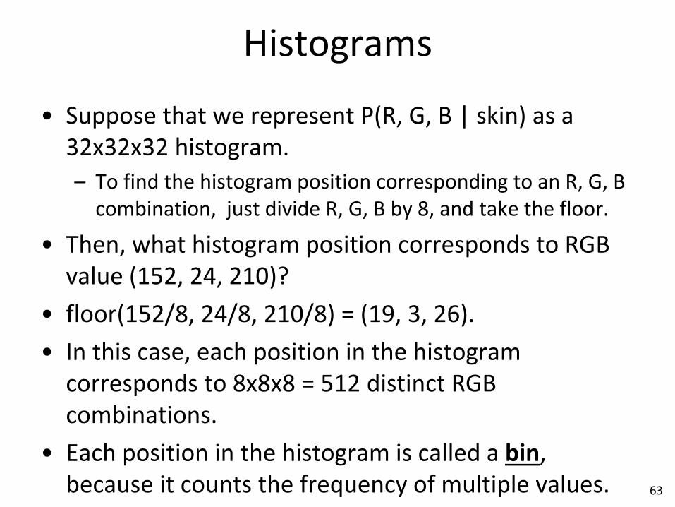
Histograms
• Suppose that we represent P(R, G, B | skin) as a 32x32x32 histogram.
– To find the histogram position corresponding to an R, G, B combination, just divide R, G, B by 8, and take the floor.
• Then, what histogram position corresponds to RGB value (152, 24, 210)?
• floor(152/8, 24/8, 210/8) = (19, 3, 26).
• In this case, each position in the histogram corresponds to 8x8x8 = 512 distinct RGB combinations.
• Each position in the histogram is called a bin, because it counts the frequency of multiple values.
63

How Many Bins?
• How do we decide the size of the histogram?
– Why 32x32x32?
– Why not 16x16x16, or 8x8x8, or 64x64x64?
64

How Many Bins?
• How do we decide the size of the histogram?
– Why 32x32x32?
– Why not 16x16x16, or 8x8x8, or 64x64x64?
• Overall, we have a tradeoff:
– Larger histograms require more training data.
– If we do have sufficient training data, larger histograms give us more information compared to smaller histograms.
– If we have insufficient training data, then larger histograms give us less reliable information than smaller histograms.
• How can we choose the size of a histogram in practice?
65

How Many Bins?
• How do we decide the size of the histogram?
– Why 32x32x32?
– Why not 16x16x16, or 8x8x8, or 64x64x64?
• Overall, we have a tradeoff:
– Larger histograms require more training data.
– If we do have sufficient training data, larger histograms give us more information compared to smaller histograms.
– If we have insufficient training data, then larger histograms give us less reliable information than smaller histograms.
• How can we choose the size of a histogram in practice?
– Just try different sizes, see which one is the most accurate in classifying test examples. 66

Limitations of Histograms
• For skin detection, histograms are a reasonable choice.
• How about the satellite image dataset?
– There, each pattern has 36 dimensions (i.e., 36 attributes).
– Each attribute is an integer between 1 and 157.
• What histogram size would make sense here?
67

Limitations of Histograms
• For skin detection, histograms are a reasonable choice.
• How about the satellite image dataset?
– There, each pattern has 36 dimensions (i.e., 36 attributes).
– Each attribute is an integer between 1 and 157.
• What histogram size would make sense here?
• Even if we discretize each attribute to just two values, we still need to compute 236 values, which is about 69 billion values.
• We have 4,435 training examples, so clearly we do not have enough data to estimate that many values.
68

The Naïve Bayes Classifier
• The naive Bayes classifier is a method that makes the (typically unrealistic) assumption that the different attributes are independent of each other.
– The naïve Bayes classifier can be combined with pretty much any probability estimation method, including histograms.
• Using the naïve Bayes approach, what histograms do we compute for the satellite image data?
69

The Naïve Bayes Classifier
• The naive Bayes classifier is a method that makes the (typically unrealistic) assumption that the different attributes are independent of each other.
– The naïve Bayes classifier can be combined with pretty much any probability estimation method, including histograms.
• Using the naïve Bayes approach, what histograms do we compute for the satellite image data?
– Instead of needing to compute a 36-dimensional histogram, we can compute 36 one-dimensional histograms.
• Why?
70

The Naïve Bayes Classifier
• The naive Bayes classifier is a method that makes the (typically unrealistic) assumption that the different attributes are independent of each other.
– The naïve Bayes classifier can be combined with pretty much any probability estimation method, including histograms.
• Using the naïve Bayes approach, what histograms do we compute for the satellite image data?
– Instead of needing to compute a 36-dimensional histogram, we can compute 36 one-dimensional histograms.
• Why? Because of independence. We can compute the probability distribution separately for each dimension.
– P(X1, X2, …, X36 | c) = ???
71

The Naïve Bayes Classifier
• The naive Bayes classifier is a method that makes the (typically unrealistic) assumption that the different attributes are independent of each other.
– The naïve Bayes classifier can be combined with pretty much any probability estimation method, including histograms.
• Using the naïve Bayes approach, what histograms do we compute for the satellite image data?
– Instead of needing to compute a 36-dimensional histogram, we can compute 36 one-dimensional histograms.
• Why? Because of independence. We can compute the probability distribution separately for each dimension.
– P(X1, X2, …, X36 | c) = P(X1 | c) * P(X2| c) * … * P(X36 | c).
72

The Naïve Bayes Classifier
• Suppose that build these 36 one-dimensional histograms.
• Suppose that we treat each value (from 1 to 157) separately, so each histogram has 157 bins.
• How many numbers do we need to compute in order to compute our P(X1, X2, …, X36 | c) distribution?
73

The Naïve Bayes Classifier
• Suppose that build these 36 one-dimensional histograms.
• Suppose that we treat each value (from 1 to 157) separately, so each histogram has 157 bins.
• How many numbers do we need to compute in order to compute our P(X1, X2, …, X36 | c) distribution?
• We need 36 histograms (one for each dimension).
– 36*157 = 5,652 values.
– Much better than 69 billion values for 236 bins.
• We compute P(X1, X2, …, X36 | c) for six different classes c, so overall we compute 36*157*6 = 33,912 values.
74

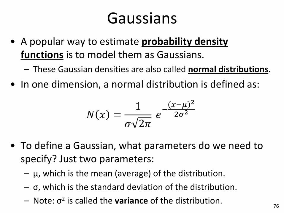
Gaussians • A popular way to estimate probability density
functions is to model them as Gaussians.
– These Gaussian densities are also called normal distributions.
• In one dimension, a normal distribution is defined as:
𝑁 𝑥 =1
𝜎 2𝜋 𝑒−𝑥−𝜇 2
2𝜎2
• To define a Gaussian, what parameters do we need to specify?
75
Gaussians • A popular way to estimate probability density
functions is to model them as Gaussians.
– These Gaussian densities are also called normal distributions.
• In one dimension, a normal distribution is defined as:
𝑁 𝑥 =1
𝜎 2𝜋 𝑒−𝑥−𝜇 2
2𝜎2
• To define a Gaussian, what parameters do we need to specify? Just two parameters:
– μ, which is the mean (average) of the distribution.
– σ, which is the standard deviation of the distribution.
– Note: σ2 is called the variance of the distribution. 76

Examples of Gaussians
77
Increasing the standard deviation makes the values more spread out.
Decreasing the std makes the distribution more peaky.
The integral is always equal to 1.
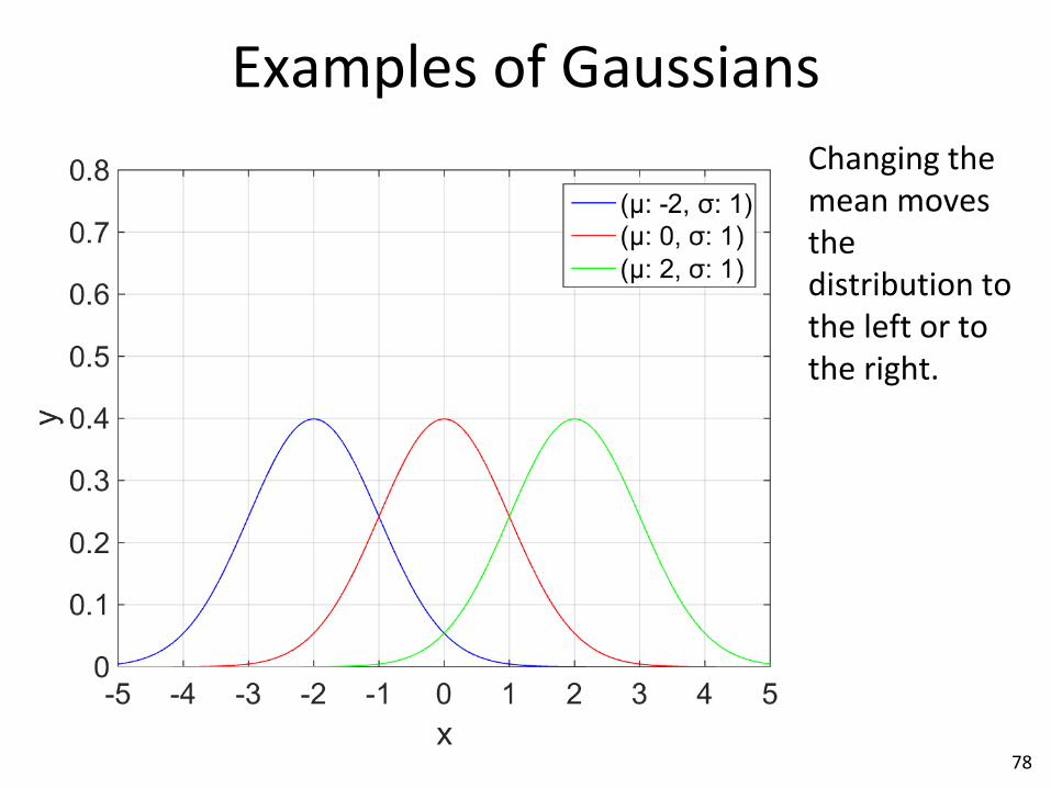
Examples of Gaussians
78
Changing the mean moves the distribution to the left or to the right.

Estimating a Gaussian
• In one dimension, a Gaussian is defined like this:
𝑁 𝑥 =1
𝜎 2𝜋 𝑒−𝑥−𝜇 2
2𝜎2
• Given a set of n real numbers x1, …, xn, we can easily find the best-fitting Gaussian for that data.
• The mean μ is simply the average of those numbers:
𝜇 =1
𝑛 𝑥𝑖
𝑛
1
• The standard deviation σ is computed as:
𝜎 =1
𝑛 − 1 (𝑥𝑖 − 𝜇)
2
𝑛
1
79

Estimating a Gaussian
• Fitting a Gaussian to data does not guarantee that the resulting Gaussian will be an accurate distribution for the data.
• The data may have a distribution that is very different from a Gaussian.
• This also happens when fitting a line to data.
– We can estimate the parameters for the best-fitting line.
– Still, the data itself may not look at all like a line.
80

Example of Fitting a Gaussian
81
The blue curve is a density function F such that:
- F(x) = 0.25 for 1 ≤ x ≤ 3.
- F(x) = 0.5 for 7 ≤ x ≤ 8.
The red curve is the Gaussian fit G to data generated using F.

Example of Fitting a Gaussian
82
Note that the Gaussian does not fit the data well.
X F(x) G(x)
1 0.25 0.031
2 0.25 0.064
3 0.25 0.107
4 0 0.149
5 0 0.172
6 0 0.164
7 0.5 0.130
8 0.5 0.085

Example of Fitting a Gaussian
83
The peak value of G is 0.173, for x=5.25.
F(5.25) = 0!!!
X F(x) G(x)
1 0.25 0.031
2 0.25 0.064
3 0.25 0.107
4 0 0.149
5 0 0.172
6 0 0.164
7 0.5 0.130
8 0.5 0.085

Example of Fitting a Gaussian
84
The peak value of F is 0.5, for 7 ≤ x ≤ 8. In that range, G(x) ≤ 0.13.
X F(x) G(x)
1 0.25 0.031
2 0.25 0.064
3 0.25 0.107
4 0 0.149
5 0 0.172
6 0 0.164
7 0.5 0.130
8 0.5 0.085

Naïve Bayes with 1D Gaussians
• Suppose the patterns come from a d-dimensional space: – Examples: the pendigits, satellite, and yeast datasets.
• Let dim(x, i) be a function that returns the value of a pattern x in the i-th dimension. – For example, if x = (v1, …, vd), then dim(x, i) returns vi.
• For each dimension i, we can use a Gaussian to model the distribution Pi(vi | c) of the data in that dimension, given their class.
• For example for the pendigits dataset, we would get 160 Gaussians: – 16 dimensions * 10 classes.
• Then, we can use the naïve Bayes approach (i.e., assume pairwise independence of all dimensions), to define P(x | c) as:
𝑃 𝑥 𝑐) = 𝑃𝑖 dim (𝑥, 𝑖) 𝑐)
𝑑
𝑖=1
85

Mixtures of Gaussians
86
• This figure shows our previous example, where we fitted a Gaussian into some data, and the fit was poor.
• Overall, Gaussians have attractive properties: – They require learning only two numbers (μ and σ), and thus require few
training data to estimate those numbers.
• However, for some data, Gaussians are just not good fits.

Mixtures of Gaussians
87
• Mixtures of Gaussians are oftentimes a better solution. – They are defined in the next slide.
• They still require relatively few parameters to estimate, and thus can be learned from relatively small amounts of data.
• They can fit pretty well actual distributions of data.
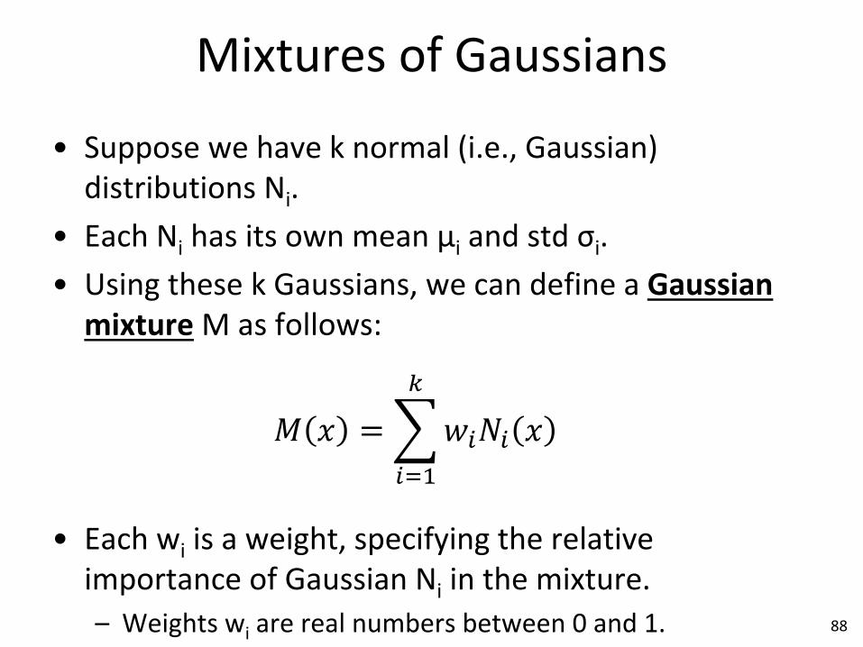
Mixtures of Gaussians
• Suppose we have k normal (i.e., Gaussian) distributions Ni.
• Each Ni has its own mean μi and std σi.
• Using these k Gaussians, we can define a Gaussian mixture M as follows:
𝑀 𝑥 = 𝑤𝑖𝑁𝑖 𝑥
𝑘
𝑖=1
• Each wi is a weight, specifying the relative importance of Gaussian Ni in the mixture.
– Weights wi are real numbers between 0 and 1.
– Weights wi must sum up to 1, so that the integral of M is 1.
88

Mixtures of Gaussians – Example
89
The blue and green curves show two Gaussians.
The red curve shows a mixture of those Gaussians.
w1 = 0.9.
w2 = 0.1.
The mixture looks a lot like N1, but is influenced a little by N2 as well.

Mixtures of Gaussians – Example
90
The blue and green curves show two Gaussians.
The red curve shows a mixture of those Gaussians.
w1 = 0.7.
w2 = 0.3.
The mixture looks less like N1 compared to the previous example, and is influenced more by N2.

Mixtures of Gaussians – Example
91
The blue and green curves show two Gaussians.
The red curve shows a mixture of those Gaussians.
w1 = 0.5.
w2 = 0.5.
At each point x, the value of the mixture is the average of N1(x) and N2(x).

Mixtures of Gaussians – Example
92
The blue and green curves show two Gaussians.
The red curve shows a mixture of those Gaussians.
w1 = 0.3.
w2 = 0.7.
The mixture now resembles N2 more than N1.

Mixtures of Gaussians – Example
93
The blue and green curves show two Gaussians.
The red curve shows a mixture of those Gaussians.
w1 = 0.1.
w2 = 0.9.
The mixture now is almost identical to N2(x).

Learning a Mixture of Gaussians
• Suppose we are given training data x1, x2, …, xn.
• Suppose all xj belong to the same class c.
• How can we fit a mixture of Gaussians to this data?
• This will be the topic of the next few slides.
• We will learn a very popular machine learning algorithm, called the EM algorithm.
– EM stands for Expectation-Maximization.
• Step 0 of the EM algorithm: pick k manually.
– Decide how many Gaussians the mixture should have.
– Any approach for choosing k automatically is beyond the scope of this class.
94

Learning a Mixture of Gaussians
• Suppose we are given training data x1, x2, …, xn.
• Suppose all xj belong to the same class c.
• We want to model P(x | c) as a mixture of Gaussians.
• Given k, how many parameters do we need to estimate in order to fully define the mixture?
• Remember, a mixture M of k Gaussians is defined as:
• For each Ni, we need to estimate three numbers: – wi, μi, σi.
• So, in total, we need to estimate 3*k numbers. 95
𝑀 𝑥 = 𝑤𝑖𝑁𝑖 𝑥
𝑘
𝑖=1
= 𝑤𝑖1
𝜎𝑖 2𝜋 𝑒−𝑥−𝜇𝑖2
2𝜎𝑖2
𝑘
𝑖=1

Learning a Mixture of Gaussians
• Suppose we are given training data x1, x2, …, xn.
• A mixture M of k Gaussians is defined as:
• For each Ni, we need to estimate wi, μi, σi.
• Suppose that we knew for each xj, that it belongs to one and only one of the k Gaussians.
• Then, learning the mixture would be a piece of cake:
• For each Gaussian Ni: – Estimate μi, σi based on the examples that belong to it.
– Set wi equal to the fraction of examples that belong to Ni. 96
𝑀 𝑥 = 𝑤𝑖𝑁𝑖 𝑥
𝑘
𝑖=1
= 𝑤𝑖1
𝜎𝑖 2𝜋 𝑒−𝑥−𝜇𝑖2
2𝜎𝑖2
𝑘
𝑖=1

Learning a Mixture of Gaussians
• Suppose we are given training data x1, x2, …, xn.
• A mixture M of k Gaussians is defined as:
• For each Ni, we need to estimate wi, μi, σi.
• However, we have no idea which mixture each xj belongs to.
• If we knew μi and σi for each Ni, we could probabilistically assign each xj to a component. – “Probabilistically” means that we would not make a hard assignment,
but we would partially assign xj to different components, with each assignment weighted proportionally to the density value Ni(xj).
97
𝑀 𝑥 = 𝑤𝑖𝑁𝑖 𝑥
𝑘
𝑖=1
= 𝑤𝑖1
𝜎𝑖 2𝜋 𝑒−𝑥−𝜇𝑖2
2𝜎𝑖2
𝑘
𝑖=1

Example of Partial Assignments
• Using our previous example of a mixture:
• Suppose xj = 6.5.
• How do we assign 6.5 to the two Gaussians?
• N1(6.5) = 0.0913.
• N2(6.5) = 0.3521.
• So:
– 6.5 belongs to N1 by 0.0913
0.0913+0.3521 = 20.6%.
– 6.5 belongs to N2 by 0.3521
0.0913+0.3521 = 79.4%.
98

The Chicken-and-Egg Problem
• To recap, fitting a mixture of Gaussians to data involves estimating, for each Ni, values wi, μi, σi.
• If we could assign each xj to one of the Gaussians, we could compute easily wi, μi, σi.
– Even if we probabilistically assign xj to multiple Gaussians, we can still easily wi, μi, σi, by adapting our previous formulas. We will see the adapted formulas in a few slides.
• If we knew μi, σi and wi, we could assign (at least probabilistically) xj’s to Gaussians.
• So, this is a chicken-and-egg problem.
– If we knew one piece, we could compute the other.
– But, we know neither. So, what do we do?
99

On Chicken-and-Egg Problems
• Such chicken-and-egg problems occur frequently in AI.
• Surprisingly (at least to people new in AI), we can easily solve such chicken-and-egg problems.
• Overall, chicken and egg problems in AI look like this: – We need to know A to estimate B.
– We need to know B to compute A.
• There is a fairly standard recipe for solving these problems.
• Any guesses?
100

On Chicken-and-Egg Problems
• Such chicken-and-egg problems occur frequently in AI.
• Surprisingly (at least to people new in AI), we can easily solve such chicken-and-egg problems.
• Overall, chicken and egg problems in AI look like this: – We need to know A to estimate B.
– We need to know B to compute A.
• There is a fairly standard recipe for solving these problems.
• Start by giving to A values chosen randomly (or perhaps non-randomly, but still in an uninformed way, since we do not know the correct values).
• Repeat this loop: – Given our current values for A, estimate B.
– Given our current values of B, estimate A.
– If the new values of A and B are very close to the old values, break.
101

The EM Algorithm - Overview
• We use this approach to fit mixtures of Gaussians to data.
• This algorithm, that fits mixtures of Gaussians to data, is called the EM algorithm (Expectation-Maximization algorithm).
• Remember, we choose k (the number of Gaussians in the mixture) manually, so we don’t have to estimate that.
• To initialize the EM algorithm, we initialize each μi, σi, and wi. Values wi are set to 1/k. We can initialize μi, σi in different ways: – Giving random values to each μi.
– Uniformly spacing the values given to each μi.
– Giving random values to each σi.
– Setting each σi to 1 initially.
• Then, we iteratively perform two steps. – The E-step.
– The M-step.
102

The E-Step
• E-step. Given our current estimates for μi, σi, and wi:
– We compute, for each i and j, the probability pij = P(Ni | xj): the probability that xj was generated by Gaussian Ni.
– How? Using Bayes rule.
𝑝𝑖𝑗 = P(𝑁𝑖|𝑥𝑗) = 𝑃 𝑥𝑗 | 𝑁𝑖 ∗𝑃(𝑁𝑖)
𝑃(𝑥𝑗)=𝑁𝑖 𝑥𝑗 ∗ 𝑤𝑖
𝑃(𝑥𝑗)
𝑁𝑖 𝑥𝑗 =1
𝜎𝑖 2𝜋 𝑒−𝑥−𝜇𝑖2
2𝜎𝑖2
𝑃 𝑥𝑗 = 𝑤𝑖′𝑁𝑖′ 𝑥𝑗
𝑘
𝑖′=1
103

The M-Step: Updating μi and σi • M-step. Given our current estimates of pij, for each i, j:
– We compute μi and σi for each Ni, as follows:
104
𝜇𝑖 = [𝑝𝑖𝑗𝑥𝑗𝑛𝑗=1 ]
𝑝𝑖𝑗𝑛𝑗=1
𝜎𝑖 = [𝑝𝑖𝑗 𝑥𝑗 − 𝜇𝑗
2]𝑛𝑗=1
𝑝𝑖𝑗𝑛𝑗=1
𝜇 =1
𝑛 𝑥𝑗
𝑛
1
𝜎 =1
𝑛 − 1 (𝑥𝑗 − 𝜇)
2
𝑛
𝑗=1
– To understand these formulas, it helps to compare them to the standard formulas for fitting a Gaussian to data:

The M-Step: Updating μi and σi
• Why do we take weighted averages at the M-step?
• Because each xj is probabilistically assigned to multiple Gaussians.
• We use 𝑝𝑖𝑗 = 𝑃 𝑁𝑖|𝑥𝑗 as weight of the assignment of xj to Ni.
105
𝜇𝑖 = [𝑝𝑖𝑗𝑥𝑗𝑛𝑗=1 ]
𝑝𝑖𝑗𝑛𝑗=1
𝜎𝑖 = [𝑝𝑖𝑗 𝑥𝑗 − 𝜇𝑗
2]𝑛𝑗=1
𝑝𝑖𝑗𝑛𝑗=1
𝜇 =1
𝑛 𝑥𝑗
𝑛
1
𝜎 =1
𝑛 − 1 (𝑥𝑗 − 𝜇)
2
𝑛
𝑗=1
– To understand these formulas, it helps to compare them to the standard formulas for fitting a Gaussian to data:

The M-Step: Updating wi
• At the M-step, in addition to updating μi and σi, we also need to update wi, which is the weight of the i-th Gaussian in the mixture.
• The formula shown above is used for the update of wi.
– We sum up the weights of all objects for the i-th Gaussian.
– We divide that sum by the sum of weights of all objects for all Gaussians.
– The division ensures that 𝑤𝑖𝑘𝑖=1 = 1.
106
𝑤𝑖 = 𝑝𝑖𝑗𝑛𝑗=1
𝑝𝑖𝑗𝑛𝑗=1
𝑘𝑖=1

The EM Steps: Summary
• E-step: Given current estimates for each μi, σi, and wi, update pij:
• M-step: Given our current estimates for each pij, update μi, σi and wi:
107
𝜇𝑖 = [𝑝𝑖𝑗 𝑥𝑗𝑛𝑗=1 ]
𝑝𝑖𝑗𝑛𝑗=1
𝜎𝑖 = [𝑝𝑖𝑗 𝑥𝑗 − 𝜇𝑗
2]𝑛𝑗=1
𝑝𝑖𝑗𝑛𝑗=1
𝑝𝑖𝑗 = 𝑁𝑖 𝑥𝑗 ∗ 𝑤𝑖
𝑃(𝑥𝑗)
𝑤𝑖 = 𝑝𝑖𝑗𝑛𝑗=1
𝑝𝑖𝑗𝑛𝑗=1
𝑘𝑖=1

The EM Algorithm - Termination
• The log likelihood of the training data is defined as:
• As a reminder, M is the Gaussian mixture, defined as:
• One can prove that, after each iteration of the E-step and the M-step, this log likelihood increases or stays the same.
• We check how much the log likelihood changes at each iteration.
• When the change is below some threshold, we stop.
108
𝑀 𝑥 = 𝑤𝑖𝑁𝑖 𝑥
𝑘
𝑖=1
= 𝑤𝑖1
𝜎𝑖 2𝜋 𝑒−𝑥−𝜇𝑖2
2𝜎𝑖2
𝑘
𝑖=1
𝐿 𝑥1, … , 𝑥𝑛 = log 2 𝑀 𝑥𝑗
𝑛
𝑗=1

The EM Algorithm: Summary
• Initialization:
– Initialize each μi and σi using your favorite approach (e.g., set each μi to a random value, and set each σi to 1).
– last_log_likelihood = -infinity.
• Main loop:
– E-step: • Given our current estimates for each μi and σi, update each pij.
– M-step: • Given our current estimates for each pij, update each μi and σi.
– log_likelihood = 𝐿 𝑥1, … , 𝑥𝑛 .
– if (log_likelihood – last_log_likelihood) < threshold, break.
– last_log_likelihood = log_likelihood
109

The EM Algorithm: Limitations
• When we fit a Gaussian to data, we always get the same result.
• We can also prove that the result that we get is the best possible result. – There is no other Gaussian giving a higher log likelihood to the data,
than the one that we compute as described in these slides.
• When we fit a mixture of Gaussians to the same data, do we always end up with the same result?
110

The EM Algorithm: Limitations
• When we fit a Gaussian to data, we always get the same result.
• We can also prove that the result that we get is the best possible result. – There is no other Gaussian giving a higher log likelihood to the data,
than the one that we compute as described in these slides.
• When we fit a mixture of Gaussians to the same data, we (sadly) do not always get the same result.
• The EM algorithm is a greedy algorithm.
• The result depends on the initialization values.
• We may have bad luck with the initial values, and end up with a bad fit.
• There is no good way to know if our result is good or bad, or if better results are possible.
111

Mixtures of Gaussians - Recap
• Mixtures of Gaussians are widely used.
• Why? Because with the right parameters, they can fit very well various types of data.
– Actually, they can fit almost anything, as long as k is large enough (so that the mixture contains sufficiently many Gaussians).
• The EM algorithm is widely used to fit mixtures of Gaussians to data.
112

Multidimensional Gaussians
• So far we have discussed Gaussians (and mixtures) for the case where our training examples x1, x2, …, xn are real numbers.
• What if each xj is a vector?
– Let D be the dimensionality of the vector.
– Then, we can write xj as (xj,1, xj,2, …, xj,D), where each xj,d is a real number.
• We can define Gaussians for vector spaces as well.
• To fit a Gaussian to vectors, we must compute two things:
– The mean (which is also a D-dimensional vector).
– The covariance matrix (which is a DxD matrix).
113

Multidimensional Gaussians - Mean
• Let x1, x2, …, xn be D-dimensional vectors.
• xj = (xj,1, xj,2, …, xj,D), where each xj,d is a real number.
• Then, the mean μ = (μ1, ..., μD) is computed as:
• Therefore, μd = 1
𝑛 𝑥𝑗,𝑑𝑛1
114
𝜇 =1
𝑛 𝑥𝑗
𝑛
1

Multidimensional Gaussians – Covariance Matrix
• Let x1, x2, …, xn be D-dimensional vectors.
• xj = (xj,1, xj,2, …, xj,D), where each xj,d is a real number.
• Let Σ be the covariance matrix. Its size is DxD.
• Let σr,c be the value of Σ at row r, column c.
115
𝜎𝑟,𝑐 =1
𝑛 − 1 (𝑥𝑗,𝑟 − 𝜇𝑟)(𝑥𝑗,𝑐 − 𝜇𝑐)
𝑛
𝑗=1

Multidimensional Gaussians – Evaluation
• Let v = (v1, v2, …, vD) be a D-dimensional vector.
• Let N be a D-dimensional Gaussian with mean μ and covariance matrix Σ.
• Let σr,c be the value of Σ at row r, column c.
• Then, the density N(v) of the Gaussian at point v is:
• |Σ| is the determinant of Σ.
• Σ−1 is the matrix inverse of Σ.
• (𝑥 − 𝜇)Τ is a 1xD row vector, 𝑥 − 𝜇 is a Dx1 column vector. 116
𝑁 𝑣 =1
2𝜋 𝐷|Σ| exp −
1
2 (𝑥 − 𝜇)ΤΣ−1(𝑥 − 𝜇)

A 2-Dimensional Example
• Here you see (from different points of view) a visualization of a two dimensional Gaussian. – Axes: x1, x2, value.
• Its peak value is on the mean, which is (0,0).
• It has a ridge directed (in the top figure) from the bottom left to the top right.
117

A 2-Dimensional Example
• The view from the top shows that, for any value A, the set of points (x, y) such that N(x, y) = A form an ellipse.
– Each value corresponds to a color.
118

Multidimensional Gaussians – Training
• Let N be a D-dimensional Gaussian with mean μ and covariance matrix Σ.
• How many parameters do we need to specify N?
– The mean μ is defined by D numbers.
– The covariance matrix Σ requires D2 numbers σr,c.
– Strictly speaking, Σ is symmetric, σr,c = σc,r.
– So, we need roughly D2/2 parameters.
• The number of parameters is quadratic to D.
• The number of training data we need for reliable estimation is also quadratic to D. 119

Gaussians: Recap
• 1-dimensional Gaussians are easy to estimate from relatively few examples.
– They are specified using only two parameters, μ and σ.
• D-dimensional Gaussians are specified using Ο(D2) parameters.
• Gaussians take a specific shape, which may not fit well the actual distribution of the data.
• Mixtures of Gaussians can take a wide range of shapes, and fit a wide range of actual distributions.
– Mixtures are fitted to data using the EM algorithm.
– The EM algorithm can be used for both one-dimensional and multi-dimensional mixtures. 120