dssat version 3 - dssat.net
TRANSCRIPT

DSSAT version 3
International Benchmark Sites Network for Agrotechnology TransferUniversity of Hawaii, Honolulu, Hawaii
Editors:
Gordon Y. TsujiGoro UeharaSharon Balas
Volume 3

IBSNAT, The International Benchmark Sites Network for Agrotechnology
Transfer, is a network consisting of the contractor (University of Hawaii),
its subcontractors and many global collaborators. Together they have
created a network of national, regional and international agricultural
research for the transfer of agrotechnology among global partners in both
developed and lesser developed countries.
From 1982 to 1987, IBSNAT was a program of the U.S. Agency for
International Development under a cost-reimbursement Contract, No.
DAN-4054-C-00-2071-00, with the University of Hawaii. From 1987 to
1993, the contract was replaced with a Cooperative Agreement, No.
DAN-4054-A-00-7081-00, between the University of Hawaii and USAID.
Correct Citation: G.Y. Tsuji, G. Uehara and S. Balas (eds.). 1994.
DSSAT v3. University of Hawaii, Honolulu, Hawaii.
Copyright University of Hawaii 1994
All reported opinions, conclusions and recommendations are those of the authors
(contractors) and not those of the funding agency or the United States govern-
L I B R A R Y O F CO N G R E S S 94-19296ISBN 1-886684-03-0 (VO L U M E 3)ISBN 1-886684-00-6 (3 VO L U M E SE T )

DSSAT V3
VO L U M E 3 -1
SE A S O N A L AN A LY S I S
VO L U M E 3 -2
SE Q U E N C E AN A LY S I S
VO L U M E 3 -3WE AT H E RMA N
VOLUME 3
VO L U M E 3 -4
GE N O T Y P E CO E F F I C I E N T
CA L C U L AT O R

i v
DSSAT v3, Volume 3 • DSSAT v3, Volume 3 • DSSAT v3, Volume 3 • DSSAT v3, Volume 3 • DSSAT v3, Volume 3 • DSSAT v3, Vo lume 3 • DSSA

v
¥ DSSAT v3, Volume 3 ¥ DSSAT v3, Volume 3 ¥ DSSAT v3, Volume 3 ¥ DSSAT v3, Volume 3 ¥ DSSAT v3, Volume 3 ¥ DSSAT v3, Volume 3 ¥ DSSAT v3, Volume
TABLE OF CONTENTS
CH A P T E R ON E. IN T R O D U C T I O N 3
SYSTEM REQUIREMENTS 4
CH A P T E R TW O. CR E A T I N G MO D E L IN P U T F I L E S F O R SE A S O N A L
AN A L Y S I S 5
CH A P T E R TH R E E . RU N N I N G SE A S O N A L AN A L Y S I S EX P E R I M E N T S 13
OVERVIEW 13
AN EXAMPLE 14
INFORMATION AND ERROR MESSAGES 17
CH A P T E R FO U R . AN A L Y Z I N G SE A S O N A L AN A L Y S I S EX P E R I M E N T S 23
OVERVIEW 23
AN EXAMPLE 24
ANALYZE BIOPHYSICAL VARIABLES 26
GRAPHICS MAIN MENU 28
ANALYZE ECONOMIC VARIABLES 34
ECONOMIC EVALUATION MAIN MENU 34
MODIFY HARDCOPY OPTIONS 44
SELECTING ANOTHER INPUT FILE FOR ANALYSIS 48
INFORMATION AND ERROR MESSAGES 48
RE F E R E N C E S 55
AP P E N D I X A. CO M B I N I N G Y I E L D A N D PR I C E D I S T R I B U T I O N S 57
AN ILLUSTRATION 58
AP P E N D I X B . TH R E E DE C I S I O N CR I T E R I A 59
MEAN-VARIANCE (EV) ANALYSIS 59
STOCHASTIC DOMINANCE (SD) ANALYSIS 59
MEAN-GINI DOMINANCE (MGD) ANALYSIS 60
AN EXAMPLE 60
VO L U M E 3 -1 . SE A S O N A L AN A LY S I S 1

v i
DSSAT v3, Volume 3 • DSSAT v3, Volume 3 • DSSAT v3, Volume 3 • DSSAT v3, Volume 3 • DSSAT v3, Volume 3 • DSSAT v3, Vo lume 3 • DSSA
F I G U R E S
FIGURE 1. STEPS IN SEASONAL ANALYSIS 4
FIGURE 2. MENU OPTIONS FOR THE SEASONAL ANALYSIS PROGRAM 23
FIGURE 3. STOCHASTIC PRICE-COST DISTRIBUTIONS 38
TA B L E S
TABLE 1. SEASONAL EXPERIMENT LISTING FILE EXP.LST 5
TABLE 2. PART OF MODEL INPUT FILE UFGA7812.SNX 7
TABLE 3. SUMMARY OUTPUT LISTING FILE SEASONAL.LST 13
TABLE 4. SUMMARY OUTPUT FILE UFGA7812.SNS (FIRST 20 DATA RECORDS ONLY) 18
TABLE 5. PRICE-COST FILE DEFAULT.PRI 37
TABLE 6. SAMPLE SECTION OF GRAPH.INI 45
TABLE 7. PRINTER TYPES SUPPORTED BY THE GRAPHICS PROGRAM 46
TABLE 8. EXPERIMENT DATA CODES FILE DATA.CDE – SUMMARYSECTION ONLY 47
TABLE 9. PART OF SEASONAL ANALYSIS RESULTS FILE UFGA7812.SNR 49

v i i
¥ DSSAT v3, Volume 3 ¥ DSSAT v3, Volume 3 ¥ DSSAT v3, Volume 3 ¥ DSSAT v3, Volume 3 ¥ DSSAT v3, Volume 3 ¥ DSSAT v3, Volume 3 ¥ DSSAT v3, Volume
VO L U M E 3 -2 . SE Q U E N C E AN A LY S I S 67
CH A P T E R ON E. IN T R O D U C T I O N 69
SYSTEM REQUIREMENTS 70
CH A P T E R TW O. CR E A T I N G MO D E L IN P U T F I L E S F O R SE Q U E N C E
AN A L Y S I S 73
FILEX FOR SEQUENCE ANALYSIS 73
TIMING CONTROLS 78
SIMULATION CONTROL OPTIONS 79
CH A P T E R TH R E E . RU N N I N G SE Q U E N C E AN A L Y S I S EX P E R I M E N T S 81
OVERVIEW 81
AN EXAMPLE 82
INFORMATION AND ERROR MESSAGES 84
CH A P T E R FO U R . AN A L Y Z I N G SE Q U E N C E AN A L Y S I S EX P E R I M E N T S 89
OVERVIEW 89
AN EXAMPLE 90
ANALYZE BIOPHYSICAL VARIABLES 93
GRAPHICS-REGRESSION MAIN MENU 96
ANALYZING MORE THAN ONE CROP AT A TIME 107
ANALYZE ECONOMIC VARIABLES 112
ECONOMIC EVALUATION MAIN MENU 112
MODIFY HARDCOPY OPTIONS 121
SELECTING ANOTHER INPUT FILE FOR ANALYSIS 126
INFORMATION AND ERROR MESSAGES 126
RE F E R E N C E S 133
AP P E N D I X . TH E ST A B I L I T Y O F OU T P U T VA R I A B L E S F R O M
RE P L I C A T E D SE Q U E N C E EX P E R I M E N T S 135
F I G U R E S
FIGURE 1. STEPS IN SEQUENCE ANALYSIS 71
FIGURE 2. MENU OPTIONS FOR THE SEQUENCE ANALYSIS PROGRAM 90

v i i i
DSSAT v3, Volume 3 • DSSAT v3, Volume 3 • DSSAT v3, Volume 3 • DSSAT v3, Volume 3 • DSSAT v3, Volume 3 • DSSAT v3, Vo lume 3 • DSSA
FIGURE 3. “SIMULATED” SEQUENCE OUTPUTS FOR N = 100, 20, 10,
AND 5, RESPECTIVELY. 136
TA B L E S
TABLE 1. SEQUENCE EXPERIMENT LISTING FILE EXP.LST 73
TABLE 2. A SAMPLE FILEX FOR CROP SEQUENCING: EBAF1101.SQX 75
TABLE 3. SUMMARY MODEL OUTPUT LISTING FILE SEQUENCE.LST 81
TABLE 4. SUMMARY OUTPUT FILE EBAF1101.SQS (FIRST 20
DATA RECORDS ONLY) 85
TABLE 5. PART OF THE DEFAULT SEQUENCE PRICE FILE, DEFAULT.PRQ 115
TABLE 6. SAMPLE SECTION OF GRAPH.INI 123
TABLE 7. PRINTER TYPES SUPPORTED BY THE GRAPHICS PROGRAM 124
TABLE 8. EXPERIMENT DATA CODES FILE DATA.CDE – SUMMARY
SECTION ONLY 125
TABLE 9. PART OF SEQUENCE ANALYSIS RESULTS FILE EPAF1101.SQR127

CH A P T E R ON E. IN T R O D U C T I O N 139
PROGRAM DESCRIPTION 139
OVERVIEW OF FUNCTIONS 140
SYSTEM REQUIREMENTS 140
CH A P T E R TW O. GE T T I N G ST A R T E D 141
STARTING WEATHERMAN 141
WEATHERMAN USER INTERFACE 141
COMMON DIALOG BOXES 144
STEPS FOR CLEANING AND CONVERTING WEATHER DATA 147
CH A P T E R TH R E E . IN T R O D U C T O R Y TU T O R I A L 149
BROWSE THE MENU AND ONLINE HELP 149
SELECT A NEW STATION 149
IMPORT DAILY WEATHER FILES 150
CALCULATE WEATHER GENERATOR PARAMETERS 152
GENERATE WEATHER DATA 152
CALCULATE STATISTICS 153
CALCULATE STATISTICS FOR THE GENERATED DATA 153
GRAPH OBSERVED DAILY TEMPERATURE 153
GRAPH STATISTICS FOR OBSERVED AND GENERATED DATA 154
EXPORT DAILY WEATHER FILES 155
CH A P T E R FO U R . WE A T H E R M A N RE F E R E N C E GU I D E 157
VARIABLES 157
FILE MENU 157
STATION MENU 160
IMPORT/EXPORT MENU 164
GENERATE MENU 173
ANALYZE MENU 179
OPTIONS MENU 186
QUIT MENU 192
VO L U M E 3 -3 . WE AT H E RMA N 137
ix
¥ DSSAT v3, Volume 3 ¥ DSSAT v3, Volume 3 ¥ DSSAT v3, Volume 3 ¥ DSSAT v3, Volume 3 ¥ DSSAT v3, Volume 3 ¥ DSSAT v3, Volume 3 ¥ DSSAT v3, Volume

x
DSSAT v3, Volume 3 • DSSAT v3, Volume 3 • DSSAT v3, Volume 3 • DSSAT v3, Volume 3 • DSSAT v3, Volume 3 • DSSAT v3, Vo lume 3 • DSSA
RE F E R E N C E S 193
AP P E N D I X A. AB B R E V I A T I O N S US E D I N WE A T H E RMA N 195
DAILY WEATHER VARIABLES 195
SUMMARY FILES 195
AP P E N D I X B . C L I M A T E F I L E FO R M A T 197
TA B L E S
TABLE 1. USER INTERFACE ITEMS AND THEIR FUNCTIONS IN
WEATHERMAN 142
TABLE 2. LIST OF ESSENTIAL STEPS FOR CREATING A COMPLETE DAILY
WEATHER DATA FILE WITH THE CORRECT FORMAT AND UNITS
FROM RAW DATA IN WEATHERMAN 148
TABLE 3. WEATHERMAN VARIABLES AND ASSOCIATED UNITS 158
TABLE 4. WEATHER STATION INFORMATION REQUIRED FOR A NEW
STATION 162
TABLE 5. EXPLANATION OF ERROR CODES USED TO FLAG SUSPECT OR
ERRONEOUS DATA 170
TABLE 6. EXPLANATION OF IMPORT OPTIONS 171
TABLE 7. EXPLANATION OF EXPORT OPTIONS 175
TABLE 8. EXPLANATION OF DATA FILL OPTIONS 176
TABLE 9. EXPLANATION OF STATISTICS TIME GROUPINGS 182

x i
¥ DSSAT v3, Volume 3 ¥ DSSAT v3, Volume 3 ¥ DSSAT v3, Volume 3 ¥ DSSAT v3, Volume 3 ¥ DSSAT v3, Volume 3 ¥ DSSAT v3, Volume 3 ¥ DSSAT v3, Volume
VO L U M E 3 -4 . GE N O T Y P E CO E F F I C I E N T
CA L C U L AT O R 201
CH A P T E R ON E. IN T R O D U C T I O N 203
PROGRAM COMPONENTS 203
SYSTEM REQUIREMENTS 207
CH A P T E R TW O. GE T T I N G ST A R T E D 209
CH A P T E R TH R E E . RU N N I N G GE NCA L C 211
DETERMINE GENETIC COEFFICIENTS 211
DISCUSSION 221
RE F E R E N C E S 223
AP P E N D I X A. GE NCA L C MO D E L RE Q U I R E M E N T S 225
AP P E N D I X B . CO N F I G U R A T I O N F I L E (DSSATPRO.FLE ) 231
AP P E N D I X C. AB B R E V I A T I O N S 233
F I G U R E
FIGURE 1. GENCALC COMPONENTS 204
TA B L E S
TABLE 1. REQUIREMENTS FOR CROP MODELS TO WORK UNDER
GENCALC 225
TABLE 2. EXAMPLE OF A CULTIVAR (GENOTYPE) COEFFICIENT FILE 227
TABLE 3. EXAMPLE OF THE REQUIRED SECTION OF THE
OVERVIEW.OUT FILE 228
TABLE 4. EXAMPLE OF AN EXPERIMENT DETAILS FILE 229
TABLE 5. EXAMPLE CONTENTS OF THE DSSATPRO.FLE FILE 232

x i i
DSSAT v3, Volume 3 • DSSAT v3, Volume 3 • DSSAT v3, Volume 3 • DSSAT v3, Volume 3 • DSSAT v3, Volume 3 • DSSAT v3, Vo lume 3 • DSSA

VO L U M E 3 -1
SEASONALANALYSIS
P.K. TH O R N T O N,G. HO O G E N B O O M,P.W. WI L K E N S ,J .W. JO N E S
INTERNATIONAL FERTILIZER DEVELOPMENT CENTER
UNIVERSITY OF GEORGIA, UNIVERSITY OF FLORIDA
INTERNATIONAL BENCHMARK SITES NETWORK FOR AGROTECHNOLOGY TRANSFER

2
Seasonal Analysis ¥ Seasonal Analysis ¥ Seasonal Analysis ¥ Seasonal Analysis ¥ Seasonal Analysis ¥ Seasonal Analysis ¥ Seasonal Analysis ¥ Seasonal Analysis ¥ Seas
DSSAT v3, Volume 3 ¥ DSSAT v3, Volume 3 ¥ DSSAT v3, Volume 3 ¥ DSSAT v3, Volume 3 ¥ DSSAT v3, Volume 3 ¥ DSSAT v3, Volume 3 ¥ DSSAT v3, Volume 3 ¥ DSSAT v3, V

• Analysis ¥ Seasonal Analysis ¥ Seasonal Analysis ¥ Seasonal Analysis ¥ Seasonal Analysis ¥ Seasonal Analysis ¥ Seasonal Analysis ¥ Seasonal Analysis ¥ Seasonal Analysis ¥
3 ¥ DSSAT v3, Volume 3 ¥ DSSAT v3, Volume 3 ¥ DSSAT v3, Volume 3 ¥ DSSAT v3, Volume 3 ¥ DSSAT v3, Volume 3 ¥ DSSAT v3, Volume 3 ¥ DSSAT v3, Volume 3 ¥ DSSAT v3,
3
CHAPTER ONE.INTRODUCTION
The Seasonal Analysis program allows the user to perform comparisons of simu-lations obtained by running the DSSAT v3 crop models with different combina-tions of inputs. A simulation experiment, which may be made up of many treat-ments and may be replicated through time using different weather years, is set upby the user, the models are run, and the user can then analyze the results usingthe seasonal analysis program. The ÒseasonalÓ aspect of the driver and analysisprograms relates to the fact that what is being run are experiments of single crop-ping seasons; while these may be replicated, there are no carry-over effects fromone season or crop to the subsequent season or crop. Those types of experimentscan be simulated and analyzed using the sequence driver and analysis programs(see Volume 3-2, Thornton et al. 1994, of this book for a description of these pro-grams).
Seasonal Analysis is useful for comparing methods of managing a crop in particu-lar environments, such as different planting dates, varieties, or fertilizer applica-tion regimes, for example. If such comparisons are made across many differenttypes of weather years, then the variability associated with crop performance, as afunction of the interactions between weather and other factors of the physicalenvironment, can be isolated and quantified. The information produced can beused to help pre-screen a wide variety of different options, the most promising ofwhich might then warrant further evaluation and, eventually, field testing.
There are three basic steps involved in Seasonal Analysis:
1. The creation of an appropriate model input file;2. Running the crop model(s) using a special controller program called the sea-sonal
analysis driver;3. Analyzing the results of the simulation using the Seasonal Analysis program.
The links between these steps are shown in Figure 1. Seasonal analyses are runfrom the DSSAT v3 Shell (see Volume 1-3, Hunt et al. 1994, of this book) under themenu item ANALYSES. The three steps are explained in Chapter 2 herein.
sis
4
Seasonal Analysis ¥ Seasonal Analysis ¥ Seasonal Analysis ¥ Seasonal Analysis ¥ Seasonal Analysis ¥ Seasonal Analysis ¥ Seasonal Analysis ¥ Seasonal Analysis ¥ Seas
DSSAT v3, Volume 3 ¥ DSSAT v3, Volume 3 ¥ DSSAT v3, Volume 3 ¥ DSSAT v3, Volume 3 ¥ DSSAT v3, Volume 3 ¥ DSSAT v3, Volume 3 ¥ DSSAT v3, Volume 3 ¥ DSSAT v3, V
FIGURE 1. STEPS IN SEASONAL ANALYSIS.
SY S T E M RE Q U I R E M E N T S
The useable portion of your systemÕs 640 Kb RAM should be at least 520 Kb insize for the models to run and for the analysis program and graphics to work.
If the driver or analysis program still does not work properly, one problem maybe associated with the number of BUFFERS and FILES defined in CONFIG.SYS.These will need to be set to at least 20 each.
Replicated seasonal simulations on an 8086 or 80286 system may take a great dealof time. In such cases, the number of replicates should be kept to a minimum.Seasonal analysis, like the rest of the DSSAT3, will operate without a mathcoprocessor, but this is not recommended
DSSATPRO.FLE
XCREATEPROGRAM
OR
ASCIITEXT
EDITOR
EXP.LSTDRIVER
PROGRAM
UFGA7812.SNX
UFGA7801.SNX
FILEXs
CROP
MODELS
OUTPUT FILES
SEASONAL.LST
SUMMARYOUTPUT
FILES
STEP 1 CREATE A FILEX
STEP 2 RUN THE EXPERIMENT
DSSATPRO.FLE
PRICE FILE(S) *.PRI
SEASONAL
ANALYSIS
PROGRAMUFGA7812.SNR
ANALYSISRESULTS
FILES
STEP 3 ANALYZE MODEL OUTPUTS
FILEX are crop model input files, listed in EXP.LST
Summary Output Files contain model outputs, and are listed in SEASONAL.LST
ANALYSIS RESULTS FILES contain the results of all analyses carried out
DSSATPRO.FLE contains path information for all components of the DSSAT v3
PRICE FILES for seasonal analysis have the extension PRI
NOTES
UFGA7812.SNS

5
• Analysis ¥ Seasonal Analysis ¥ Seasonal Analysis ¥ Seasonal Analysis ¥ Seasonal Analysis ¥ Seasonal Analysis ¥ Seasonal Analysis ¥ Seasonal Analysis ¥ Seasonal Analysis ¥
3 ¥ DSSAT v3, Volume 3 ¥ DSSAT v3, Volume 3 ¥ DSSAT v3, Volume 3 ¥ DSSAT v3, Volume 3 ¥ DSSAT v3, Volume 3 ¥ DSSAT v3, Volume 3 ¥ DSSAT v3, Volume 3 ¥ DSSAT v3,
sis
The program XCreate (see Volume 1-4, Imamura 1994, of this book for a descrip-tion of this program) can be used to create model input files (FILEXs) for runningseasonal analyses. (For a description of FILEX, see Volume 2-1, Jones et al. 1994,of this book.) Alternatively, these files can be created using an ASCII text editor.The advantage of using the program XCreate is that the experiment listing fileEXP.LST is updated automatically (see Volume 2-1, Jones et al. 1994, of this bookfor a description of EXP.LST). If you create a seasonal analysis FILEX yourselfusing an ASCII editor, then you must either update EXP.LST yourself, or run theFile Manager Utility program (by opening the SEASONAL Ñ ÒInputsÓ menuitems of the DSSAT v3 Shell) for the FILEX to be accessible to the seasonal analy-sis driver.
Seasonal analysis model input files created with XCreate have the extension SNX.You may also put FILEXs that refer to a particular crop in EXP.LST, using theÒExperimentÓ option mode of FILEX creation found in the XCreate program.Thus you could run a FILEX called UFGA9201.MZX, as long as this file was listedin the listing file EXP.LST in the directory that contains the seasonal analysisinput files, which is usually DSSAT3\SEASONAL (see Table 1 for an example ofthe EXP.LST file).
CHAPTER TWO.CREATING MODEL INPUT FILES FOR
SEASONAL ANALYSIS
TABLE 1. SEASONAL EXPERIMENT LISTING FILE EXP.LST.
*EXPERIMENT LIST
@# FILENAME EXT ENAME1 UFGA7801 SNX GAINESVILLE, SOYBEAN, IRRIGATED AND RAINFED2 UFGA7802 SNX EXAMPLE SEASONAL ANALYSIS, SB+MZ3 UFGA7805 SNX PLANTING DATE EXPERIMENT, 1978 BRAGG, GNV4 UFGA8201 SNX GAINESVILLE, FLORIDA, MAIZE, IR*N-FERT5 UFGA7812 SNX GAINESVILLE, FLORIDA, SB IRRIGATION EXPERIMENT

6
Seasonal Analysis ¥ Seasonal Analysis ¥ Seasonal Analysis ¥ Seasonal Analysis ¥ Seasonal Analysis ¥ Seasonal Analysis ¥ Seasonal Analysis ¥ Seasonal Analysis ¥ Seas
DSSAT v3, Volume 3 ¥ DSSAT v3, Volume 3 ¥ DSSAT v3, Volume 3 ¥ DSSAT v3, Volume 3 ¥ DSSAT v3, Volume 3 ¥ DSSAT v3, Volume 3 ¥ DSSAT v3, Volume 3 ¥ DSSAT v3, V
An example of a seasonal analysis FILEX is shown in Table 2. Though not all of theSIMULATION CONTROL blocks of FILEX appear in Table 2, you can print a fulllisting of this file, UFGA7812.SNX, found on the DSSAT v3 distribution diskette.Refer to the shaded portions in Table 2 when reading the following paragraphs.
In the *TREATMENTS section of the file, treatments are specified as for a regularexperiment. You need to ensure that the treatment numbers are in ascending, con-secutive order (treatment numbers are specified in the two columns with header@N). In Seasonal Analysis, the options ÒR,Ó ÒOÓ and ÒCÓ should always be left attheir default values of 1, 0 and 0, respectively.
Because the example experiment UFGA7812SN is a comparison of automatic irriga-tion schedules, the example found in Table 2 requires 6 simulation control sections,as specified by the simulation control factor levels SM, under *TREATMENTS.
In the *SIMULATION CONTROLS blocks in Table 2, there are a number of simula-tion control options that are generally important for Seasonal Analyses. These aredescribed as follows.
NYERSNYERS is the number of replicates for the experiment and should have a valuebetween 1 and 30. You may need to check the availability of historical weather datafiles if you are running a number of replicates and the weather data switch WTHER(one of the METHODS options found in the *SIMULATION CONTROLS block) isset to ÒMÓ (measured). In this case, make sure that you have at least NYERS+1complete years of historical weather data available. Most often, seasonal analysesare run using simulated weather with this switch set to ÒWÓ (as set in Table 2) orÒS.Ó ÒWÓ is for the WGEN (Richardson and Wright 1984) weather generator andÒSÓ is for the SIMMETEO (Geng et al. 1988) weather generator. In either of thesecases, the climate file for the site (with extension CLI) will be used by the model.
NREPSNREPS should be left at the default value of 1. It has no meaning for SeasonalAnalysis.
RSEEDRSEED is the random number seed for weather generation. RSEED is used only ifthe WTHER option is set to ÒWÓ or ÒS.Ó If you start a simulation from the samestarting date (SDATE) with the same seed, you will obtain the same sequence ofrandom numbers, and hence the same sequence of daily weather.
7
Analysis ¥ Seasonal Analysis ¥ Seasonal Analysis ¥ Seasonal Analysis ¥ Seasonal Analysis ¥ Seasonal Analysis ¥ Seasonal Analysis ¥ Seasonal Analysis ¥ Seasonal Analysis ¥
3 ¥ DSSAT v3, Volume 3 ¥ DSSAT v3, Volume 3 ¥ DSSAT v3, Volume 3 ¥ DSSAT v3, Volume 3 ¥ DSSAT v3, Volume 3 ¥ DSSAT v3, Volume 3 ¥ DSSAT v3, Volume 3 ¥ DSSAT v3,
sis
TABLE 2. PART OF MODEL INPUT FILE UFGA7812.SNX.
*EXP.DETAILS: UFGA7812SN GAINESVILLE, FLORIDA, SB IRRIGATION EXPERIMENT
*TREATMENTS ——————-FACTOR LEVELS——————@N R O C TNAME.....................CU FL SA IC MP MI MF MR MC MT ME MH SM1 1 0 0 RAINFED 1 1 0 1 1 0 0 1 0 0 0 0 12 1 0 0 AUTOMATIC 90% 1 1 0 1 1 0 0 1 0 0 0 0 23 1 0 0 AUTOMATIC 70% 1 1 0 1 1 0 0 1 0 0 0 0 34 1 0 0 AUTOMATIC 50% 1 1 0 1 1 0 0 1 0 0 0 0 45 1 0 0 AUTOMATIC 30% 1 1 0 1 1 0 0 1 0 0 0 0 56 1 0 0 AUTOMATIC 10% 1 1 0 1 1 0 0 1 0 0 0 0 6
*CULTIVARS@C CR INGENO CNAME1 SB IB0001 BRAGG
*FIELDS@L ID_FIELD WSTA.... FLSA FLOB FLDT FLDD FLDS FLST SLTX SLDP ID_SOIL1 UFGA0001 UFGA7801 -99 0 IB000 0 0 00000 -99 180 IBSB910015
*INITIAL CONDITIONS@C PCR ICDAT ICRT ICND ICRN ICRE1 SB 78166 100 -99 1.00 1.00
@C ICBL SH2O SNH4 SNO31 5 0.086 0.6 1.51 15 0.086 0.6 1.51 30 0.086 0.6 1.51 45 0.086 0.6 1.51 60 0.086 0.6 1.51 90 0.076 0.6 0.61 120 0.076 0.6 0.51 150 0.130 0.6 0.51 180 0.258 0.6 0.5
*PLANTING DETAILS@P PDATE EDATE PPOP PPOE PLME PLDS PLRS PLRD PLDP PLWT PAGE PENV PLPH1 78166 -99 29.9 29.9 S R 91 0 4.0 -99 -99 -99.0 -99.0
*RESIDUES AND OTHER ORGANIC MATERIALS@R RDATE RCOD RAMT RESN RESP RESK RINP RDEP1 78166 IB001 1000 0.80 -9.00 -9.00 100 15
*SIMULATION CONTROLS@N GENERAL NYERS NREPS START SDATE RSEED SNAME....................1 GE 20 1 S 78166 9875
@N OPTIONS WATER NITRO SYMBI PHOSP POTAS DISES1 OP Y Y Y N N N
@N METHODS WTHER INCON LIGHT EVAPO INFIL PHOTO1 ME W M E R S C
@N MANAGEMENT PLANT IRRIG FERTI RESID HARVS1 MA R N R R M
@N OUTPUTS FNAME OVVEW SUMRY FROPT GROTH CARBN WATER NITRO MINER DISES LONG1 OU Y N A 10 N N N N N N N

8
Seasonal Analysis ¥ Seasonal Analysis ¥ Seasonal Analysis ¥ Seasonal Analysis ¥ Seasonal Analysis ¥ Seasonal Analysis ¥ Seasonal Analysis ¥ Seasonal Analysis ¥ Seas
DSSAT v3, Volume 3 ¥ DSSAT v3, Volume 3 ¥ DSSAT v3, Volume 3 ¥ DSSAT v3, Volume 3 ¥ DSSAT v3, Volume 3 ¥ DSSAT v3, Volume 3 ¥ DSSAT v3, Volume 3 ¥ DSSAT v3, V
@ AUTOMATIC MANAGEMENT@N PLANTING PFRST PLAST PH2OL PH2OU PH2OD PSTMX PSTMN1 PL 155 200 40 100 30 40 10
@N IRRIGATION IMDEP ITHRL ITHUR IROFF IMETH IRAMT IREFF1 IR 30 50 100 IB001 IB001 10 0.75
@N NITROGEN NMDEP NMTHR NAMNT NCODE NAOFF1 NI 30 50 25 IB001 IB001
@N RESIDUES RIPCN RTIME RIDEP1 RE 100 1 20
@N HARVEST HFRST HLAST HPCNP HPCNR1 HA 0 365 100 0
@N GENERAL NYERS NREPS START SDATE RSEED SNAME....................2 GE 20 1 S 78166 9875
@N OPTIONS WATER NITRO SYMBI PHOSP POTAS DISES2 OP Y Y Y N N N
@N METHODS WTHER INCON LIGHT EVAPO INFIL PHOTO2 ME W M E R S C
@N MANAGEMENT PLANT IRRIG FERTI RESID HARVS2 MA R A R R M
@N OUTPUTS FNAME OVVEW SUMRY FROPT GROTH CARBN WATER NITRO MINER DISES LONG2 OU Y N A 10 N N N N N N N
@ AUTOMATIC MANAGEMENT@N PLANTING PFRST PLAST PH2OL PH2OU PH2OD PSTMX PSTMN2 PL 155 200 40 100 30 40 10
@N IRRIGATION IMDEP ITHRL ITHUR IROFF IMETH IRAMT IREFF2 IR 30 90 100 IB001 IB001 10 0.75
@N NITROGEN NMDEP NMTHR NAMNT NCODE NAOFF2 NI 30 50 25 IB001 IB001
@N RESIDUES RIPCN RTIME RIDEP2 RE 100 1 20
@N HARVEST HFRST HLAST HPCNP HPCNR2 HA 0 365 100 0
@N GENERAL NYERS NREPS START SDATE RSEED SNAME....................6 GE 20 1 S 78166 9875
@N OPTIONS WATER NITRO SYMBI PHOSP POTAS DISES6 OP Y Y Y N N N
@N METHODS WTHER INCON LIGHT EVAPO INFIL PHOTO6 ME W M E R S C
@N MANAGEMENT PLANT IRRIG FERTI RESID HARVS6 MA R A R R M
@N OUTPUTS FNAME OVVEW SUMRY FROPT GROTH CARBN WATER NITRO MINER DISES LONG6 OU Y N A 10 N N N N N N N

9
• Analysis ¥ Seasonal Analysis ¥ Seasonal Analysis ¥ Seasonal Analysis ¥ Seasonal Analysis ¥ Seasonal Analysis ¥ Seasonal Analysis ¥ Seasonal Analysis ¥ Seasonal Analysis ¥
3 ¥ DSSAT v3, Volume 3 ¥ DSSAT v3, Volume 3 ¥ DSSAT v3, Volume 3 ¥ DSSAT v3, Volume 3 ¥ DSSAT v3, Volume 3 ¥ DSSAT v3, Volume 3 ¥ DSSAT v3, Volume 3 ¥ DSSAT v3,
sis
@ AUTOMATIC MANAGEMENT@N PLANTING PFRST PLAST PH2OL PH2OU PH2OD PSTMX PSTMN6 PL 155 200 40 100 30 40 10
@N IRRIGATION IMDEP ITHRL ITHUR IROFF IMETH IRAMT IREFF6 IR 30 10 100 IB001 IB001 10 0.75
@N NITROGEN NMDEP NMTHR NAMNT NCODE NAOFF6 NI 30 50 25 IB001 IB001
@N RESIDUES RIPCN RTIME RIDEP6 RE 100 1 20
@N HARVEST HFRST HLAST HPCNP HPCNR6 HA 0 365 100 0

10
Seasonal Analysis ¥ Seasonal Analysis ¥ Seasonal Analysis ¥ Seasonal Analysis ¥ Seasonal Analysis ¥ Seasonal Analysis ¥ Seasonal Analysis ¥ Seasonal Analysis ¥ Seas
DSSAT v3, Volume 3 ¥ DSSAT v3, Volume 3 ¥ DSSAT v3, Volume 3 ¥ DSSAT v3, Volume 3 ¥ DSSAT v3, Volume 3 ¥ DSSAT v3, Volume 3 ¥ DSSAT v3, Volume 3 ¥ DSSAT v3, V
FNAMEFNAME is one of the OUTPUTS switches found in the *SIMULATION CON-TROLS blocks. If this switch is set to ÒN,Ó then the summary output file from themodel runs will be named SUMMARY.SNS. If FNAME is set to ÒY,Ó then thesummary output file name will be the same as the model FILEX name, except thatthe last letter of the extension will be changed from ÒXÓ to ÒS.Ó Thus, for theexperiment FILEX shown in Table 2 which has the name UFGA7812.SNX, thesummary output file will be named UFGA7812.SNS since the switch FNAME isset to ÒY.Ó
SUMRYSUMRY is one of the OUTPUTS switches found in the *SIMULATION CON-TROLS blocks. For seasonal simulations, this controller should always be set toÒAÓ (append); otherwise the summary output file will be successively overwrit-ten by each treatment and earlier outputs will be lost. In Table 2, the other OUT-PUT switches are set to ÒNÓ to prevent within-season output from the models.Since seasonal simulations with many replicates can produce prodigious quanti-ties of output data, it makes sense to turn these output files off, unless you needthem specifically.
You should note that if there are multiple simulation control sections in FILEX,then the driver program will use the values of NYERS, WTHER, RSEED, FNAMEand SUMRY that pertain to the lowest valid simulation control level in the file. Inother words, the value of NYERS, the number of replicates, in the lowest simula-tion control factor level (SM=1), is used for all other treatments; in Table 2, forexample, NYERS is set to 20. You could not, therefore, run an experiment thathas 4 replicates for Treatment 1 and 10 replicates for Treatment 2, for instance; thiswould not make much sense anyway.
For the specific experiment in Table 2, the first treatment is set up as a rainfedtreatment (see *TREATMENTS). Thus the IRRIG switch, which is a MANAGE-MENT option in the *SIMULATION CONTROLS block is set to ÒNÓ for Òno irri-gationÓ in block 1(i.e., N=1).
For subsequent treatments, automatic irrigation is to be applied, but the thresholdat which water is applied, in terms of the percentage of soil water in the profile, ischanged; this is the primary experimental variable. In the second *SIMULATION

11
• Analysis ¥ Seasonal Analysis ¥ Seasonal Analysis ¥ Seasonal Analysis ¥ Seasonal Analysis ¥ Seasonal Analysis ¥ Seasonal Analysis ¥ Seasonal Analysis ¥ Seasonal Analysis ¥
3 ¥ DSSAT v3, Volume 3 ¥ DSSAT v3, Volume 3 ¥ DSSAT v3, Volume 3 ¥ DSSAT v3, Volume 3 ¥ DSSAT v3, Volume 3 ¥ DSSAT v3, Volume 3 ¥ DSSAT v3, Volume 3 ¥ DSSAT v3,
sis
CONTROLS block (i.e., N=2) in Table 2, the IRRIG switch is set to ÒAÓ for Òauto-maticÓ. The corresponding information in the AUTOMATIC MANAGEMENTsection of the file, under IRRIGATION, shows that IMDEP is set to 30 and ITHRLto 90. Thus irrigation will be applied automatically when available soil water isless than or equal to a value of 90 percent (ITHRL) of what the soil can hold in thetop 30 cm of the profile (IMDEP).Compare this with the *SIMULATION CONTROLS block number 6 (i.e., N=6))where, under AUTOMATIC MANAGEMENT, ITHRL has a value of 10 (i.e., thesoil water trigger will operate when available water reaches 10 percent of fieldcapacity in the top 30 cm). Note that all other switches in each of the SIMULA-TION CONTROLS blocks in Table 2 are the same.
In general, you may mix crops in a seasonal analysis FILEX. Thus you can com-pare performance of different crops in the same experiment. Treatment 1 mightinvolve maize, and Treatment 2 dry bean, for example.

12
Seasonal Analysis ¥ Seasonal Analysis ¥ Seasonal Analysis ¥ Seasonal Analysis ¥ Seasonal Analysis ¥ Seasonal Analysis ¥ Seasonal Analysis ¥ Seasonal Analysis ¥ Seas
DSSAT v3, Volume 3 ¥ DSSAT v3, Volume 3 ¥ DSSAT v3, Volume 3 ¥ DSSAT v3, Volume 3 ¥ DSSAT v3, Volume 3 ¥ DSSAT v3, Volume 3 ¥ DSSAT v3, Volume 3 ¥ DSSAT v3, V

13
• Analysis ¥ Seasonal Analysis ¥ Seasonal Analysis ¥ Seasonal Analysis ¥ Seasonal Analysis ¥ Seasonal Analysis ¥ Seasonal Analysis ¥ Seasonal Analysis ¥ Seasonal Analysis ¥
3 ¥ DSSAT v3, Volume 3 ¥ DSSAT v3, Volume 3 ¥ DSSAT v3, Volume 3 ¥ DSSAT v3, Volume 3 ¥ DSSAT v3, Volume 3 ¥ DSSAT v3, Volume 3 ¥ DSSAT v3, Volume 3 ¥ DSSAT v3,
sis
CHAPTER THREE.RUNNING SEASONAL ANALYSIS EXPERIMENTS
OV E RV I E W
The seasonal analysis driver program takes the FILEX selected or created by theuser, and runs through each treatment in the experiment, calling the appropriatecrop model. It is very important to understand that the seasonal driver can beused for any experiment that does not involve a sequence. Thus, as far as the dri-ver is concerned, it makes no difference if FILEX describes a real 10-treatment sin-gle year experiment, or if it describes a hypothetical 4-treatment simulationexperiment to be replicated twenty times. The driver can thus be used to gener-ate replicated experiment output files, or it may simply be used to run all thetreatments pertaining to a real-world experiment automatically.
The driver is a FORTRAN program that allows the user to pick a specific entryfrom EXP.LST (i.e., a particular FILEX; see Volume 2-1, Jones et al. 1994, of thisbook for a description of EXP.LST). This FILEX is then read and various controlsare set. Each treatment specified in this FILEX is then run in its order of appear-ance in the *TREATMENTS section of the FILEX. The appropriate model is calledfor each treatment (the model is run under the command of the driver program),and it will be run for as many replicates as are specified by NYERS in the FILEX.When all the treatments of the selected simulation or real-world experiment havebeen run, the results listing file SEASONAL.LST (see the example in Table 3) isupdated with the name and description of the summary output file produced.The user can then quit the program or choose another FILEX for running with theseasonal driver.
The seasonal driver can be run in a stand-alone mode or through the DSSAT v3Shell (see Volume 3-1, Hunt et al. 1994, of this book for a description of the Shell).
TABLE 3. SUMMARY OUTPUT LISTING FILE SEASONAL.LST.
*SEASONAL LIST
@# FILENAME EXT ENAME
1 UFGA7801 SNS GAINESVILLE, SOYBEAN, IRRIGATED AND RAINFED2 UFGA7802 SNS EXAMPLE SEASONAL ANALYSIS, SB+MZ3 UFGA7812 SNS GAINESVILLE, FLORIDA, SB IRRIGATION EXPERIMENT

14
Seasonal Analysis ¥ Seasonal Analysis ¥ Seasonal Analysis ¥ Seasonal Analysis ¥ Seasonal Analysis ¥ Seasonal Analysis ¥ Seasonal Analysis ¥ Seasonal Analysis ¥ Seas
DSSAT v3, Volume 3 ¥ DSSAT v3, Volume 3 ¥ DSSAT v3, Volume 3 ¥ DSSAT v3, Volume 3 ¥ DSSAT v3, Volume 3 ¥ DSSAT v3, Volume 3 ¥ DSSAT v3, Volume 3 ¥ DSSAT v3, V
It is important to note that in whichever mode the driver is run, the programexpects to find all the model program(s) in the same directory. In the case of theDSSAT v3 Shell, this will generally be the C:\DSSAT3 directory. If model exe-cutable files are not found in that directory, then an error message is printed andthe user must arrange the executable files so that this condition is met. The fileDSSATPRO.FLE (see the Appendix to Volume 1 of this book for a description ofthis file) is also expected to be in this same directory, with appropriate pointers tothe relevant directories.
From within DSSAT v3, the current directory for seasonal runs will generally beDSSAT3\SEASONAL, where such files as EXP.LST, SEASONAL.LST and appro-priate FILEXs are stored.
The file EXP.LST may contain up to 99 experiments, a limit imposed by the filestructure. Up to 99 treatments may be simulated using the driver (again a limitimposed by FILEX), but it should be noted that the seasonal analysis program hasa limit of handling a maximum of 20 treatments and 30 replicates (i.e., a total of600 separate model runs).
AN EX A M P L E
On activating the ÒSimulateÓ option under the ÒSeasonalÓ window (Screen 1, fol-lowing page) from the DSSAT v3 Shell main menu item ANALYSES, the driverprogram is activated, and after an introductory screen the user is presented withthe following screen (Screen 2, following page). Screen 2 contains the contents ofthe file EXP.LST, the listing file in the current directory of selected FILEXs for sea-sonal analysis. This lists the file name, crop group code (generally ÒSNÓ for sea-sonal analysis, although it may be any valid crop code), and a file description.The description may be up to 60 characters long; if it is shorter, the description ispadded with full stops. The file description is obtained from columns 26 through85 of the first line of FILEX (see Table 2).
If the colors on the screen are difficult to see (such as when the program is beingrun on a monochrome laptop computer), you can force the program to displayscreens in monochrome by pressing the <ALT>-<F2> keys. Note that you cannotreverse the color scheme during a session with the program, nor is your prefer-ence stored from one session to another.
Use the mouse or cursor arrow keys to choose the Gainesville soybean irrigationexperiment FILEX, UFGA7812.SNX (used in the example in Table 2). If the cho-sen FILEX cannot be found, an error message is printed on the screen, and themenu reappears for making another choice.
15
• Analysis ¥ Seasonal Analysis ¥ Seasonal Analysis ¥ Seasonal Analysis ¥ Seasonal Analysis ¥ Seasonal Analysis ¥ Seasonal Analysis ¥ Seasonal Analysis ¥ Seasonal Analysis ¥
3 ¥ DSSAT v3, Volume 3 ¥ DSSAT v3, Volume 3 ¥ DSSAT v3, Volume 3 ¥ DSSAT v3, Volume 3 ¥ DSSAT v3, Volume 3 ¥ DSSAT v3, Volume 3 ¥ DSSAT v3, Volume 3 ¥ DSSAT v3,
sis
S SeasonalQ Sequence
DECISION SUPPORT SYSTEM FOR AGROTECHNOLOGY TRANSFER
DATA MODEL ANALYSES TOOLS SETUP/QUIT
ESCmoves through menu choicesmoves to higher menu level Version: 3.0
↑ ↓ → ←
C Create
I Inputs
S Simulate
O Outputs
A Analyze
Run the appropriate crop model(s) using a controlling 'driver' program.
SCREEN 1.
DSSAT Version 3.0 Cropping Season Analysis
FILE EXT ENAME
UFGA7801 SNX GAINESVILLE, SOYBEAN, IRRIGATED AND RAINFED........
UFGA7802 SNX EXAMPLE SEASONAL ANALYSIS, SB+M2...................
UFGA7805 SNX PLANTING DATE EXPERIMENT, 1978 BRAGG, GNV..........
UFGA8201 SNX GAINESVILLE, FLORIDA, MAIZE, IR*N-FERT.............
UFGA7812 SNX GAINESVILLE, FLORIDA, SB IRRIGATION EXPERIMENT.....
F1 (Help) 306432 Mem
SCREEN 2.

16
Seasonal Analysis ¥ Seasonal Analysis ¥ Seasonal Analysis ¥ Seasonal Analysis ¥ Seasonal Analysis ¥ Seasonal Analysis ¥ Seasonal Analysis ¥ Seasonal Analysis ¥ Seas
DSSAT v3, Volume 3 ¥ DSSAT v3, Volume 3 ¥ DSSAT v3, Volume 3 ¥ DSSAT v3, Volume 3 ¥ DSSAT v3, Volume 3 ¥ DSSAT v3, Volume 3 ¥ DSSAT v3, Volume 3 ¥ DSSAT v3, V
Once a valid FILEX name is selected, the driver checks to see if there is an exist-ing output file with the same name in the current directory (this is controlledwithin FILEX, see above). If there is, then the user is warned that the output filewill be overwritten. Press <Y> to continue regardless, or <N> to quit the pro-gram to allow you to rename or move the existing output file.
Once past Screen 2, the driver will issue appropriate commands and call up thecrop model(s). The initial model-produced screen warns the user not to touch thekeyboard. Once simulations are under way, each model run is summarized onthe screen, so that the user can chart progress of the experiment (Screen 3, below,shows the first 20 simulations associated with model input file UFGA7812.SNX).Experiments with many treatments and/or many replicates may take a great dealof time to simulate, especially on older personal computers. No keyboard inputshould be made, unless an error occurs, until the simulations have finished.
To abort the simulation runs before they have finished, press the <ESC> key or<CTRL-BREAK>.
For each FILEX simulated, the driver updates or creates a listing file which storesthe names of the summary results files (in similar fashion to EXP.LST, whichstores the names of available FILEXs in the current directory). This file, SEASON-AL.LST, is of the same format (Table 3), and is used by the analysis programdescribed in the next section. Two other messages may appear on the finalscreen:
SCREEN 3.

17
• Analysis ¥ Seasonal Analysis ¥ Seasonal Analysis ¥ Seasonal Analysis ¥ Seasonal Analysis ¥ Seasonal Analysis ¥ Seasonal Analysis ¥ Seasonal Analysis ¥ Seasonal Analysis ¥
3 ¥ DSSAT v3, Volume 3 ¥ DSSAT v3, Volume 3 ¥ DSSAT v3, Volume 3 ¥ DSSAT v3, Volume 3 ¥ DSSAT v3, Volume 3 ¥ DSSAT v3, Volume 3 ¥ DSSAT v3, Volume 3 ¥ DSSAT v3,
sis
1. If FNAME was set to ÒN,Ó then the summary output file produced by themodel(s), SUMMARY.OUT, was renamed to SUMMARY.SNS; the programtells you that this has been done;
2. If the summary output file of the appropriate name does not appear in SEA-SONAL.LST, then SEASONAL.LST is updated, and the program tells you thatthis has been done.
Press any key to continue. You will then be asked if you want to run anotherexperiment. Respond by pressing the <N> or <ENTER> keys to exit the pro-gram, or the <Y> key to return to the opening screen showing file EXP.LST, whereanother experiment can be chosen and simulated (see Screen 2). You may simu-late as many FILEXs as you like, one after the other, without exiting the driverprogram.
Simulation results are stored in the summary output file, in this exampleUFGA7812.SNS. The first 20 simulation records of this file are shown in Table 4.
IN F O R M AT I O N AN D ER R O R ME S S A G E S
A number of information and error messages are produced by the driver pro-gram. In the list that follows, each message is preceded by a single-digit code anda three digit message/error number. If the single-digit code is Ò0,Ó then this is afatal error, and the program exits. If the code is Ò1,Ó then the program will contin-ue, as the error may not be fatal. Information messages have code Ò1Ó also.
0 001 Cannot find experiment file.The FILEX experiment listing file could not be found in the current directory.
0 002 No entries found in file.The FILEX experimental listing file was found, but it contains no valid entries.
1 003 Cannot find file :The specified file cannot be found (non-fatal).
0 004 Error reading :An undefined read error occurred when attempting to read the file. The problemis usually caused by incorrect format of the file.
0 005 No valid treatments found in file.No valid treatments were found in the FILEX selected.

18
Seasonal Analysis ¥ Seasonal Analysis ¥ Seasonal Analysis ¥ Seasonal Analysis ¥ Seasonal Analysis ¥ Seasonal Analysis ¥ Seasonal Analysis ¥ Seasonal Analysis ¥ Seas
DSSAT v3, Volume 3 ¥ DSSAT v3, Volume 3 ¥ DSSAT v3, Volume 3 ¥ DSSAT v3, Volume 3 ¥ DSSAT v3, Volume 3 ¥ DSSAT v3, Volume 3 ¥ DSSAT v3, Volume 3 ¥ DSSAT v3, V
TABLE 4. SUMMARY OUTPUT FILE UFGA7812.SNS, FIRST 20 DATA RECORDS ONLY.
Columns 1-86
*SUMMARY : UFGA7812SN GAINESVILLE, FLORIDA, SB IRRIGATION EXPERIMENT
!IDENTIFIERS...............................DATES......................... DRY WEIGHTS.@RP TN ROC CR TNAM FNAM SDAT PDAT ADAT MDAT HDAT DWAP CWAM1 1 100 SB RAINFED UFGA0001 78166 78166 78213 78282 78294 67 58802 1 100 SB RAINFED UFGA0001 79166 79166 79212 79284 79296 67 74893 1 100 SB RAINFED UFGA0001 80166 80166 80212 80282 80294 67 66924 1 100 SB RAINFED UFGA0001 81166 81166 81212 81287 81299 67 59315 1 100 SB RAINFED UFGA0001 82166 82166 82212 82283 82295 67 71756 1 100 SB RAINFED UFGA0001 83166 83166 83213 83285 83297 67 58027 1 100 SB RAINFED UFGA0001 84166 84166 84213 84285 84297 67 62038 1 100 SB RAINFED UFGA0001 85166 85166 85213 85284 85296 67 63929 1 100 SB RAINFED UFGA0001 86166 86166 86212 86285 86297 67 698610 1 100 SB RAINFED UFGA0001 87166 87166 87212 87282 87294 67 698011 1 100 SB RAINFED UFGA0001 88166 88166 88213 88284 88296 67 663212 1 100 SB RAINFED UFGA0001 89166 89166 89212 89284 89296 67 556613 1 100 SB RAINFED UFGA0001 90166 90166 90213 90283 90295 67 640314 1 100 SB RAINFED UFGA0001 91166 91166 91212 91282 91294 67 644815 1 100 SB RAINFED UFGA0001 92166 92166 92213 92283 92295 67 703016 1 100 SB RAINFED UFGA0001 93166 93166 93212 93283 93295 67 690017 1 100 SB RAINFED UFGA0001 94166 94166 94212 94283 94295 67 490518 1 100 SB RAINFED UFGA0001 95166 95166 95212 95283 95295 67 711019 1 100 SB RAINFED UFGA0001 96166 96166 96212 96283 96295 67 678720 1 100 SB RAINFED UFGA0001 97166 97166 97212 67279 97291 67 4863
Columns 87-176
....................................WATER.....................................NITROGEN....HWAM HWAH BWAH HWUM H#AM H#UM IR#M IRCM PRCM ETCM ROCM DRCM SWXM NI#M NICM3565 3565 3924 171 2083 2.05 0 0 834 509 35 365 84 0 03166 3166 3526 143 2218 2.05 0 0 904 489 38 419 117 0 02939 2939 2992 163 1806 2.05 0 0 502 452 1 70 138 0 03602 3602 3573 183 1972 2.05 0 0 718 491 8 243 135 0 02942 2942 2860 174 1695 2.05 0 0 833 479 11 390 111 0 03415 3415 2788 165 2070 2.05 0 0 611 466 13 150 141 0 03210 3210 3181 166 1934 2.05 0 0 513 455 9 117 90 0 03280 3280 3706 177 1849 2.05 0 0 872 486 22 431 92 0 03214 3214 3766 171 1878 2.05 0 0 557 487 5 153 71 0 03329 3329 3304 170 1953 2.05 0 0 445 449 1 39 115 0 02808 2808 2759 163 1719 2.05 0 0 462 446 1 81 92 0 03253 3253 3149 162 2013 2.05 0 0 819 501 43 309 125 0 03140 3140 3309 142 2213 2.05 0 0 527 432 27 145 80 0 03457 3457 3573 175 1973 2.05 0 0 803 481 13 365 101 0 03388 3388 3512 161 2104 2.05 0 0 534 473 3 128 89 0 02287 2287 2618 155 1474 2.05 0 0 493 423 4 68 157 0 03521 3521 3588 169 2081 2.05 0 0 828 517 20 305 144 0 03479 3479 3308 184 1894 2.05 0 0 684 478 27 252 86 0 01798 1798 3064 105 1705 2.05 0 0 689 412 29 309 98 0 0
19
• Analysis ¥ Seasonal Analysis ¥ Seasonal Analysis ¥ Seasonal Analysis ¥ Seasonal Analysis ¥ Seasonal Analysis ¥ Seasonal Analysis ¥ Seasonal Analysis ¥ Seasonal Analysis ¥
3 ¥ DSSAT v3, Volume 3 ¥ DSSAT v3, Volume 3 ¥ DSSAT v3, Volume 3 ¥ DSSAT v3, Volume 3 ¥ DSSAT v3, Volume 3 ¥ DSSAT v3, Volume 3 ¥ DSSAT v3, Volume 3 ¥ DSSAT v3,
sis
Columns 177-252
................................... ORGANIC MATTER... PHOSPHORUS............NFXM NUCM NLCM NIAM CNAM GNAM RECM ONAM OCAM PO#M POCM CPAM SPAM280 18 21 27 214 185 1000 3836 39 0 0 0 0337 18 19 27 265 227 1000 3838 39 0 0 0 0302 18 21 27 235 202 1000 3836 39 0 0 0 0288 34 3 28 220 187 1000 3837 39 0 0 0 0321 26 14 28 263 229 1000 3834 39 0 0 0 0292 17 19 28 219 187 1000 3838 39 0 0 0 0310 27 8 30 250 217 1000 3837 39 0 0 0 0301 30 6 29 241 204 1000 3837 39 0 0 0 0329 17 23 26 251 209 1000 3835 39 0 0 0 0313 23 9 31 243 205 1000 3838 39 0 0 0 0308 34 1 29 249 212 1000 3837 39 0 0 0 0282 29 4 29 207 179 1000 3839 39 0 0 0 0308 19 17 29 238 207 1000 3836 39 0 0 0 0303 24 8 31 240 200 1000 3838 39 0 0 0 0316 24 18 26 256 220 1000 3835 39 0 0 0 0311 28 7 31 251 216 1000 3836 39 0 0 0 0254 29 3 31 176 146 1000 3839 39 0 0 0 0324 23 17 29 262 224 1000 3833 39 0 0 0 0331 20 15 29 260 222 1000 3838 39 0 0 0 0240 16 17 27 150 115 1000 3841 39 0 0 0 0

20
Seasonal Analysis ¥ Seasonal Analysis ¥ Seasonal Analysis ¥ Seasonal Analysis ¥ Seasonal Analysis ¥ Seasonal Analysis ¥ Seasonal Analysis ¥ Seasonal Analysis ¥ Seas
DSSAT v3, Volume 3 ¥ DSSAT v3, Volume 3 ¥ DSSAT v3, Volume 3 ¥ DSSAT v3, Volume 3 ¥ DSSAT v3, Volume 3 ¥ DSSAT v3, Volume 3 ¥ DSSAT v3, Volume 3 ¥ DSSAT v3, V
0 006 Error in *SIMULATION CONTROL factor levels.The FILEX specified by the user is defective in one of the following ways: a)FNAME was not set or not found; b) NREPS was not set or not found; or c) thesimulation control factor level with the lowest number specified by the user didnot have a corresponding *SIMULATION CONTROLS block in the file.
0 007 Error in *CULTIVAR factor levels in file :A cultivar factor level was specified in the selected FILEX that did not have a cor-responding cultivar description in the *CULTIVARS section of the file.
1 008 Model runs completed!
1 009 SUMMARY.OUT renamed to SUMMARY.SNS.
1 010 SEASONAL.LST updated, added file.Specified summary output file added to the listing file.
0 011 A required file was not found .. aborting.This usually refers to the absence of the file DSSATPRO.FLE, which could not befound.
0 012 Excessive path length error.You need to reduce the path length as specified in DSSATPRO.FLE for the cropmodel ÒccÓ (e.g. MZ). Path lengths as specified in the DSSATPRO.FLE must beless than 36 characters in total length, including drive letter, colon, and leadingand trailing slashes (\). If these paths are modified using the SETUP menu of theDSSAT v3 Shell (see Volume 1-3, Hunt et al. 1994, of this book for a description ofthe SETUP menu), then there is no problem, as the screens will not allow you toenter paths longer than this. If you modify DSSATPRO.FLE with a text editor,then you need to ensure that this total length is not exceeded.
0 013 No code error.The crop code specified (e.g. MZ) could not be found in the file DSSATPRO.FLE.This will occur if a cultivar is specified in FILEX that does not have a valid cropcode.
0 014 Read error in file :An undefined read error occurred when reading the specified file; check the for-mat of the file.
0 020 A problem was encountered executing another program.The driver was not able to execute another program. Check the free RAM thatyou have on your computer, and increase it if possible by unloading unnecessaryresident programs (e.g., a network).

21
• Analysis ¥ Seasonal Analysis ¥ Seasonal Analysis ¥ Seasonal Analysis ¥ Seasonal Analysis ¥ Seasonal Analysis ¥ Seasonal Analysis ¥ Seasonal Analysis ¥ Seasonal Analysis ¥
3 ¥ DSSAT v3, Volume 3 ¥ DSSAT v3, Volume 3 ¥ DSSAT v3, Volume 3 ¥ DSSAT v3, Volume 3 ¥ DSSAT v3, Volume 3 ¥ DSSAT v3, Volume 3 ¥ DSSAT v3, Volume 3 ¥ DSSAT v3,
sis
0 021 A problem was encountered erasing a file.The specified file could not be erased.
0 022 A problem was encountered copying a file.The specified file could not be copied successfully.
1 055 Problem in finding the appropriate help screen.The required help screen or the help screen file, SEADRV.HLP, could not befound.
1 100 Error!Undetermined error.

22
Seasonal Analysis ¥ Seasonal Analysis ¥ Seasonal Analysis ¥ Seasonal Analysis ¥ Seasonal Analysis ¥ Seasonal Analysis ¥ Seasonal Analysis ¥ Seasonal Analysis ¥ Seas
DSSAT v3, Volume 3 ¥ DSSAT v3, Volume 3 ¥ DSSAT v3, Volume 3 ¥ DSSAT v3, Volume 3 ¥ DSSAT v3, Volume 3 ¥ DSSAT v3, Volume 3 ¥ DSSAT v3, Volume 3 ¥ DSSAT v3, V

23
• Analysis ¥ Seasonal Analysis ¥ Seasonal Analysis ¥ Seasonal Analysis ¥ Seasonal Analysis ¥ Seasonal Analysis ¥ Seasonal Analysis ¥ Seasonal Analysis ¥ Seasonal Analysis ¥
3 ¥ DSSAT v3, Volume 3 ¥ DSSAT v3, Volume 3 ¥ DSSAT v3, Volume 3 ¥ DSSAT v3, Volume 3 ¥ DSSAT v3, Volume 3 ¥ DSSAT v3, Volume 3 ¥ DSSAT v3, Volume 3 ¥ DSSAT v3,
sis
Having produced a summary simulation output file from a seasonal experiment,the next step is to analyze this and compare treatments (these treatments may ormay not be replicated, but in seasonal analysis there will usually be a number ofreplicates). A brief overview of the analysis programÕs capabilities follows,together with some general usage notes. It should be noted that the analysis pro-gram can handle a maximum size of 30 replicates or 20 treatments.
Figure 2 shows the major menu options available. The program does the follow-ing.
Biophysical Analysis. Calculates means, standard deviations, maxima andminima by treatment for any or all of the 35 summary output file variables.These can be plotted as box plots, cumulative function plots, or as mean-variancediagrams. All graphs can be screen dumped to a printer or output to a file forplotting.
Economic Analysis. Calculates means, standard deviations, maxima andminima by treatment of economic returns, and plots these as box plots, cumula-tive function plots, or mean-variance diagrams. Prices and costs can be changedwithin a session, and price-cost variability can be included in the analysis.
CHAPTER FOUR.ANALYZING SEASONAL ANALYSIS EXPERIMENTS
OV E RV I E W
PERFORMSTRATEGY ANALYSIS
PLOT GRAPHS
TABULATE
SUMMARY STATISTICS
CALUCULATE ECON-OMIC RETURNS
EDIT PRICEFILE
ACCESS APRICE FILE
PLOT GRAPHS
QUIT BIOPHYSICALANALYSIS
SELECT OUTPUTVARIABLE(S)
CALCULATE & TABULATESUMMARY STATISTICS
ECONOMIC ANAYLSIS
SELECT MODELOUTPUT FILE
SELECT GRAPHICSHARDCOPY OPTIONS
FIGURE 2. MENU OPTIONS FOR THE SEASONAL ANALYSIS PROGRAM.

24
Seasonal Analysis ¥ Seasonal Analysis ¥ Seasonal Analysis ¥ Seasonal Analysis ¥ Seasonal Analysis ¥ Seasonal Analysis ¥ Seasonal Analysis ¥ Seasonal Analysis ¥ Seas
DSSAT v3, Volume 3 ¥ DSSAT v3, Volume 3 ¥ DSSAT v3, Volume 3 ¥ DSSAT v3, Volume 3 ¥ DSSAT v3, Volume 3 ¥ DSSAT v3, Volume 3 ¥ DSSAT v3, Volume 3 ¥ DSSAT v3, V
AN EX A M P L E
S SeasonalQ Sequence
DECISION SUPPORT SYSTEM FOR AGROTECHNOLOGY TRANSFER
DATA MODEL ANALYSES TOOLS SETUP/QUIT
ESCmoves through menu choicesmoves to higher menu level Version: 3.0
↑ ↓ → ←
C Create
I Inputs
S Simulate
O Outputs
A Analyze
<None> Analyze model outputs.
SCREEN 4.
Formal strategy evaluation of all treatments, if required, is carried out usingmean-Gini stochastic dominance (see Appendix B herein).Any number of summary output files can be analyzed during one session withthe program. The user can also control the type and format of hardcopy outputsfrom the graphics produced.
While these analyses are being performed, results are written to a results file. Atthe completion of the session, the user can access this file and use the data con-tained within in any way required. For example, it could be edited for importinginto a graphics, spreadsheet or statistics program.
The Seasonal Analysis program is called from the ANALYSES main menu of theDSSAT v3 Shell (Screen 4, below) and then from the ÒSeasonalÓÐÓAnalyzeÓ sub-menus. After an introductory screen, the main menu appears on Screen 5 (on fol-lowing page).
First you must select a cropping season file to analyze (i.e., a summary output filefrom a previously-run simulation). On selecting this item, the program searchesSEASONAL.LST, the listing file that contains the available model summary out-put files in the current directory (see Table 3). These are presented to the user (seeScreen 6, on following page). Note that the entries in SEASONAL.LST do not
<None> Analyze model outputs.

25
Analysis ¥ Seasonal Analysis ¥ Seasonal Analysis ¥ Seasonal Analysis ¥ Seasonal Analysis ¥ Seasonal Analysis ¥ Seasonal Analysis ¥ Seasonal Analysis ¥ Seasonal Analysis ¥
3 ¥ DSSAT v3, Volume 3 ¥ DSSAT v3, Volume 3 ¥ DSSAT v3, Volume 3 ¥ DSSAT v3, Volume 3 ¥ DSSAT v3, Volume 3 ¥ DSSAT v3, Volume 3 ¥ DSSAT v3, Volume 3 ¥ DSSAT v3,
sis
F1 (Help) 214240 Mem
Main Menu
FILE
UFGA7801 SNS GAINESVILLE, SOYBEAN, IRRIGATED AND RAINFED ........
UFGA7802 SNS EXAMPLE SEASONAL ANALYSIS, SB+MZ ...................
UFGA7812 SNS GAINESVILLE, FLORIDA, SB IRRIGATION EXPERIMENT .....
Modify hardcopy options
About VARAN2 ....
Exit
DSSAT Version 3.0 Cropping Season Analysis Tool
EXT ENAME
SCREEN 5.
SCREEN 6.
have to match the entries in EXP.LST, either in number or in order; youmay have run and analyzed the experiments in a different order, for exam-ple.
As for the driver program, if the colors on the screen are difficult to see(such as when the program is being run on a monochrome laptop comput-
F1 (Help) 214240 Mem
Main Menu
Select a cropping season file for analysis
Analyse Biophysical variables
Analyse Economic variables
Modify hardopy options
About VARAN2....
Exit
DSSAT Version 3.0 Cropping Season Analysis Tool

26
Seasonal Analysis ¥ Seasonal Analysis ¥ Seasonal Analysis ¥ Seasonal Analysis ¥ Seasonal Analysis ¥ Seasonal Analysis ¥ Seasonal Analysis ¥ Seasonal Analysis ¥ Seas
DSSAT v3, Volume 3 ¥ DSSAT v3, Volume 3 ¥ DSSAT v3, Volume 3 ¥ DSSAT v3, Volume 3 ¥ DSSAT v3, Volume 3 ¥ DSSAT v3, Volume 3 ¥ DSSAT v3, Volume 3 ¥ DSSAT v3, V
er), you can force the program to display screens in monochrome by pressing the<ALT>-<F2> keys. Again, note that you cannot reverse the color scheme duringa session with the program, nor is your preference stored from one session toanother.
Use the mouse or cursor keys to select the third file, UFGA7812.SNS, in Screen 6.After the file is selected, the program gives the user the opportunity to change thename of the analysis results file. By default, this file name will be the same as thesummary output file, except the last letter of the extension will be ÒRÓ (forÒresultsÓ). Note that file names are preserved across all three steps of the season-al analysis procedure: if the model FILEX is UFGA7812.SNX, then simulationresults from the model(s) are saved in UFGA7812.SNS, and analysis results inUFGA7812.SNR. If you want to change the results file name, enter a new name (8characters maximum). Do not add the extension; this is added automatically, andcannot be changed, and will always be ÒccRÓ where ÒccÓ is the crop code (usuallySN for seasonal analysis).
The next screen presented (Screen 7, on following page) summarizes the simula-tion runs found in the chosen summary output file. The experiment code, cropgroup and file title are displayed, with a treatment-by-treatment listing of treat-ment title, file ID, the number of replicates, and the appropriate crop pertainingto each treatment. If there are problems with the summary output file, forinstance an unequal number of replicates because of model failure for some rea-son in some treatments, these problems will usually be apparent at this stage.Such errors are usually trapped by the analysis program and result in a warningmessage to the user and termination of the program.
Press any key to continue, and the main menu of the Analysis program appearsagain (Screen 5). The items in this menu are illustrated in turn.
AN A LY Z E B I O P H Y S I C A L VA R I A B L E SOn choosing the main menu option, ÒAnalyze Biophysical Variables,Ó in Screen 5,with the mouse or cursor keys, a list of the variables available for analysisappears (Screen 8, on following page). This is a listing of all the 35 output vari-ables written to the summary output file. You can scroll up and down this listusing the <> and <¯> keys on the keyboard. Choose variable number 9, ÒHARYIELD kg/ha (i.e., harvest yield),Ó in Screen 8 by placing the cursor bar over thevariable in the list and select it by pressing the space bar. A tick mark in thebracket to the right of the variable indicates that this is the variable selected. Thespace bar can be used to toggle the selection off and on.

27
• Analysis ¥ Seasonal Analysis ¥ Seasonal Analysis ¥ Seasonal Analysis ¥ Seasonal Analysis ¥ Seasonal Analysis ¥ Seasonal Analysis ¥ Seasonal Analysis ¥ Seasonal Analysis ¥
3 ¥ DSSAT v3, Volume 3 ¥ DSSAT v3, Volume 3 ¥ DSSAT v3, Volume 3 ¥ DSSAT v3, Volume 3 ¥ DSSAT v3, Volume 3 ¥ DSSAT v3, Volume 3 ¥ DSSAT v3, Volume 3 ¥ DSSAT v3,
sis
File Title: GAINESVILLE, FLORIDA, SB IRRIGATION EXPERIMENTExperiment Code: UFGA7812 Crop Group: SN Runs : 120 Replications : 20
Treat Title Field Reps Crop
1 RAINFED............ UFGA00012 AUTOMATIC 90%...... UFGA00013 AUTOMATIC 70%...... UFGA00014 AUTOMATIC 50%...... UFGA00015 AUTOMATIC 30%...... UFGA00016 AUTOMATIC 10%...... UFGA0001
202020202020
SBSBSBSBSBSB
DSSAT Version 3.0 Cropping Season Analysis Tool
F1 (Help) Press any key to continue.. 214240 Mem
SCREEN 7.
Select a cropping season file for analysis
Analyse Biological variables
Analyse Economic variables
Modify hardopy options
About VARAN2....
Exit
F1 (Help) 214240 Mem
Main Menu
DSSAT Version 3.0 Cropping Season Analysis Tool
Analysis1
2
3
4
5
6
7
8
9
10
11
12
13
14
15
16
17
18
START SIM day [ ]
PLANTING day [ ]
ANTHESIS day [ ]
MATURITY day [ ]
HARVET day [ ]
SOWING WT kg/ha [ ]
TOPS WT. kg/ha [ ]
MAT YIELD kg/ha [ ]
HAR YIELD kg/ha [ ]
BYPRODUCT kg/ha [ ]
WEIGHT mg/unit [ ]
NUMBER #/m2 [ ]
NUMBER #/unit [ ]
IRRIG APPS # [ ]
IRRIG mm [ ]
PRECIP mm [ ]
ET TOTAL mm [ ]
RUNOFF mm [ ]
↑ ↓
SCREEN 8.
√

28
Seasonal Analysis ¥ Seasonal Analysis ¥ Seasonal Analysis ¥ Seasonal Analysis ¥ Seasonal Analysis ¥ Seasonal Analysis ¥ Seasonal Analysis ¥ Seasonal Analysis ¥ Seas
DSSAT v3, Volume 3 ¥ DSSAT v3, Volume 3 ¥ DSSAT v3, Volume 3 ¥ DSSAT v3, Volume 3 ¥ DSSAT v3, Volume 3 ¥ DSSAT v3, Volume 3 ¥ DSSAT v3, Volume 3 ¥ DSSAT v3, V
Select a cropping season file for analysis
Analyse Biological variables
Analyse Economic variables
Modify hardopy options
About VARAN2....
Exit
F1 (Help) 214240 Mem
Main Menu
DSSAT Version 3.0 Cropping Season Analysis Tool
Analysis1
2
3
4
5
6
7
8
9
10
11
12
13
14
15
16
17
18
START SIM day [ ]
PLANTING day [ ]
ANTHESIS day [ ]
MATURITY day [ ]
HARVET day [ ]
SOWING WT kg/ha [ ]
TOPS WT. kg/ha [ ]
MAT YIELD kg/ha [ ]
HAR YIELD kg/ha [ ]
BYPRODUCT kg/ha [ ]
WEIGHT mg/unit [ ]
NUMBER #/m2 [ ]
NUMBER #/unit [ ]
IRRIG APPS # [ ]
IRRIG mm [ ]
PRECIP mm [ ]
ET TOTAL mm [ ]
RUNOFF mm [ ]
↑ ↓
Variable : HAR YIELD kg/ha
Treatment
1 RAINFED............ UFGA0001 SB 3134.9 443.9 1798.0 3602.02 AUTOMATIC 90%...... UFGA0001 SB 3529.2 144.1 3219.0 3761.03 AUTOMATIC 70%...... UFGA0001 SB 3528.3 145.7 3219.0 3761.04 AUTOMATIC 50%...... UFGA0001 SB 3539.8 122.9 3249.0 3759.05 AUTOMATIC 30%...... UFGA0001 SB 3506.1 109.9 3241.0 3725.06 AUTOMATIC 10%...... UFGA0001 SB 3228.0 287.0 2530.0 3602.0
Field Crop Mean St.Dev. Min Max
Press any key to continue..
SCREEN 9.
The program calculates various statistics and presents them on screen (see Screen9, above). These values show, by treatment, the mean, standard deviation, mini-mum, and maximum harvest yield obtained from running the soybean simula-tion model. Screen 9 shows the results obtained from the simulation of the auto-matic irrigation experiment at Gainesville, Florida, UFGA7812.SNX, and referredto above. As might be expected for this simulation, mean soybean yieldincreased as the irrigation threshold increased (i.e., more water was applied tothe crop).
Press any key to continue, and the Graphics main menu appears (Screen 10, onfollowing page). Three types of graphs can be plotted, described as follows.
GR A P H I C S MA I N ME N U
OPTION 1. BOX PLOT
If this option is selected in Screen 10, a list of all the treatments is presented ( bydefault, all treatments are selected for plotting box plots when this option isselected). All of the treatments can be selected at once by pressing the <+> key, orthey can be selected individually by using the space bar as described beforeunder Screen 8. (To deselect all treatments, press the <-> key.) After treatmentselection (use the default for this example), press the <ENTER> key and a boxplot appears (see Screen 11, on second following page). This is a way of assessingvisually the variability of the output variable under consideration. For the distri-
214240 Mem

29
• Analysis ¥ Seasonal Analysis ¥ Seasonal Analysis ¥ Seasonal Analysis ¥ Seasonal Analysis ¥ Seasonal Analysis ¥ Seasonal Analysis ¥ Seasonal Analysis ¥ Seasonal Analysis ¥
3 ¥ DSSAT v3, Volume 3 ¥ DSSAT v3, Volume 3 ¥ DSSAT v3, Volume 3 ¥ DSSAT v3, Volume 3 ¥ DSSAT v3, Volume 3 ¥ DSSAT v3, Volume 3 ¥ DSSAT v3, Volume 3 ¥ DSSAT v3,
sis
Select a cropping season file for analysis
Analyse Biological variables
Analyse Economic variables
Modify hardopy options
About VARAN2....
Exit
F1 (Help) 214240 Mem
Main Menu
DSSAT Version 3.0 Cropping Season Analysis Tool
Analysis
↑ ↓
1
2
3
4
5
6
7
8
9
10
11
12
13
14
15
16
17
18
START SIM day [ ]
PLANTING day [ ]
ANTHESIS day [ ]
MATURITY day [ ]
HARVET day [ ]
SOWING WT kg/ha [ ]
TOPS WT. kg/ha [ ]
MAT YIELD kg/ha [ ]
HAR YIELD kg/ha [ ]
BYPRODUCT kg/ha [ ]
WEIGHT mg/unit [ ]
NUMBER #/m2 [ ]
NUMBER #/unit [ ]
IRRIG APPS # [ ]
IRRIG mm [ ]
PRECIP mm [ ]
ET TOTAL mm [ ]
RUNOFF mm [ ]
HAR YIELD kg/ha
Box plot
Cumulative function plot
Mean-Variance plot
Quit ...
SCREEN 10.
bution of the variable for each treatment selected, the 0th (the lowest single shortline), 25th (the lower of the short lines connected by the vertical bar), 50th (thestar), 75th (the upper of the short lines connected by the vertical bar), and 100th(the upper single short line) percentiles are plotted. Visually, these box plots aresometimes clearer than cumulative probability curves if there are many treat-ments. The 50th percentile is the median of each output variable distribution, notthe mean; but for symmetrical distributions, the median will often not differgreatly from the mean value. Note the effect of irrigation treatment on the distri-bution of soybean yield.
This graph may be plotted on your printer by pressing the <P> key while thegraph is on the screen. If the graph does not plot, you may need to change hard-copy settings (refer to the section below, ÒGraphics Hardcopy SetupÓ).Depending on the printer and the resolution used, there may be a delay of a fewseconds while this is done; wait for the graph to show on the screen again beforecontinuing.
NOTE: To return to the Analysis program from any graph, press any key.
OPTION 2. CUMULATIVE FUNCTION PLOT
When this option is selected in Screen 10, output variables by treatment are plot-
√

30
Seasonal Analysis ¥ Seasonal Analysis ¥ Seasonal Analysis ¥ Seasonal Analysis ¥ Seasonal Analysis ¥ Seasonal Analysis ¥ Seasonal Analysis ¥ Seasonal Analysis ¥ Seas
DSSAT v3, Volume 3 ¥ DSSAT v3, Volume 3 ¥ DSSAT v3, Volume 3 ¥ DSSAT v3, Volume 3 ¥ DSSAT v3, Volume 3 ¥ DSSAT v3, Volume 3 ¥ DSSAT v3, Volume 3 ¥ DSSAT v3, V
ted as cumulative function plots. (Cumulative function plots are sometimescalled cumulative probability function (CPF) plots or cumulative distributionfunction plots Ð these are the same.) Here, the output distribution for each treat-ment is ordered from smallest to largest, and plotted against equal increments ofcumulative probability.
After selecting this option, the treatment selection screen appears, allowing theuser to select which treatments are to be plotted in this way (see Screen 12, on fol-
HWAH
1 2 3 4 5 6
BOX PLOT OF HAR YIELD kg/ha
4.200k
3.600k
3.000k
2.400k
1.800k
HAR YIELD kg/ha
TREATMENT
✳
✳ ✳ ✳ ✳
✳
0 7
SCREEN 11.
HWAH
1 2 3 4 5 6 0
HAR YIELD kg/ha

31
• Analysis ¥ Seasonal Analysis ¥ Seasonal Analysis ¥ Seasonal Analysis ¥ Seasonal Analysis ¥ Seasonal Analysis ¥ Seasonal Analysis ¥ Seasonal Analysis ¥ Seasonal Analysis ¥
3 ¥ DSSAT v3, Volume 3 ¥ DSSAT v3, Volume 3 ¥ DSSAT v3, Volume 3 ¥ DSSAT v3, Volume 3 ¥ DSSAT v3, Volume 3 ¥ DSSAT v3, Volume 3 ¥ DSSAT v3, Volume 3 ¥ DSSAT v3,
sis
lowing page). A maximum of six cumulative function plots may be graphed atany time, and you can select or deselect all the treatments at once with the <+> or<-> key (as described before under Screen 8), or individual treatments with thespace bar. If more than six treatments are selected, the program will plot the firstsix treatments selected, and the rest will be ignored.
For the example, keep all treatments selected (as illustrated in Screen 12) andpress the <ENTER> key. The resulting plot is shown in Screen 13 (on followingpage). To print the graphs, press the <P> key; press the <ENTER> key to returnto the Graphics main menu (Screen 10)
OPTION 3. MEAN-VARIANCE PLOT
When this option in Screen 10 is selected, output variables may be plotted inmean-variance space. The calculated mean is plotted against the variance for theoutput variable of interest, and the treatment numbers themselves are drawn onthe graph. A maximum of 20 treatments may be plotted in this way. Such graphsare another way of giving an indication of the relative variability associated witheach treatment, and are useful for visualizing the tradeoffs that must sometimesbe made between striving for a higher mean value while increasing the variability(as described by the variance) for the output of interest.
Choose the mean-variance plot option to produce the plot (Screen 14, on secondfollowing page). Note the high variance and comparatively low mean for the
Select a cropping season file for analysis
Analyse Biological variables
Analyse Economic variables
Modify hardopy options
About VARAN2....
Exit
1
2
3
4
5
6
7
8
9
10
11
12
13
14
15
16
17
18
START SIM day [ ]
PLANTING day [ ]
ANTHESIS day [ ]
MATURITY day [ ]
HARVET day [ ]
SOWING WT kg/ha [ ]
TOPS WT. kg/ha [ ]
MAT YIELD kg/ha [ ]
HAR YIELD kg/ha [ ]
BYPRODUCT kg/ha [ ]
WEIGHT mg/unit [ ]
NUMBER #/m2 [ ]
NUMBER #/unit [ ]
IRRIG APPS # [ ]
IRRIG mm [ ]
PRECIP mm [ ]
ET TOTAL mm [ ]
RUNOFF mm [ ]
F1 (Help) 214240 Mem
Main Menu
DSSAT Version 3.0 Cropping Season Analysis Tool
Analysis
↑ ↓
HAR YIELD kg/ha
Box plot
Cumulative function plot
Mean-Variance plot
Quit ...
CPF Graph - 6 Max
1 RAINFED............ UFGA0001 [√]2 AUTOMATIC 90%...... UFGA0001 [√]3 AUTOMATIC 70%...... UFGA0001 [√]4 AUTOMATIC 50%...... UFGA0001 [√]5 AUTOMATIC 30%...... UFGA0001 [√]6 AUTOMATIC 10%...... UFGA0001 [√]
SCREEN 12.

32
Seasonal Analysis ¥ Seasonal Analysis ¥ Seasonal Analysis ¥ Seasonal Analysis ¥ Seasonal Analysis ¥ Seasonal Analysis ¥ Seasonal Analysis ¥ Seasonal Analysis ¥ Seas
DSSAT v3, Volume 3 ¥ DSSAT v3, Volume 3 ¥ DSSAT v3, Volume 3 ¥ DSSAT v3, Volume 3 ¥ DSSAT v3, Volume 3 ¥ DSSAT v3, Volume 3 ¥ DSSAT v3, Volume 3 ¥ DSSAT v3, V
rainfed treatment, Treatment Number 1. There is little to choose betweenTreatments 2, 3, and 4, in terms of their mean and variance. It seems fairly clearthat if the irrigation threshold is at least 50 percent of field capacity, then soybeanyields are not limited by water availability in this experiment.
SCREEN 13.
1.200k 1.800k 2.400k 3.000k 3.600k 4.200k
HAR YIELD kg/ha
1.000
0.800
0.600
0.400
0.200
CUMULATIVE PROBABILITY
CPF PLOT OF HAR
(1) TRT1(1) TRT3(1) TRT5
(1) TRT2(1) TRT4(1) TRT6
TRT1 TRT5
TRT3TRT2
TRT4
TRT6
HARV YIELD kg/ha
CUMULATIVE PROBABILITY

33
• Analysis ¥ Seasonal Analysis ¥ Seasonal Analysis ¥ Seasonal Analysis ¥ Seasonal Analysis ¥ Seasonal Analysis ¥ Seasonal Analysis ¥ Seasonal Analysis ¥ Seasonal Analysis ¥
3 ¥ DSSAT v3, Volume 3 ¥ DSSAT v3, Volume 3 ¥ DSSAT v3, Volume 3 ¥ DSSAT v3, Volume 3 ¥ DSSAT v3, Volume 3 ¥ DSSAT v3, Volume 3 ¥ DSSAT v3, Volume 3 ¥ DSSAT v3,
sis
The y-axis for such a plot is always scaled automatically, and care will sometimesbe needed in interpretation, as the difference between the means (i.e., the differ-ence from the top to the bottom of the scale) may not be very much, and willsometimes be much less than appears from a cursory glance at the graph. Toprint the plot, press the <P> key, or press the <ENTER> key to return to theGraphics main menu (Screen 10).
VARIANCE
MEAN
0.0k 30.0k 60.0k 90.0k 120.0k 150.0k 180.0k 210.0k
3.600k
3.500k
3.400k
3.300k
3.200k
423
5
6
E-V PLOT OF HAR YIELD kg/ha
1
HWAH
SCREEN 14.
MEAN
VARIANCE
HWAH

34
Seasonal Analysis ¥ Seasonal Analysis ¥ Seasonal Analysis ¥ Seasonal Analysis ¥ Seasonal Analysis ¥ Seasonal Analysis ¥ Seasonal Analysis ¥ Seasonal Analysis ¥ Seas
DSSAT v3, Volume 3 ¥ DSSAT v3, Volume 3 ¥ DSSAT v3, Volume 3 ¥ DSSAT v3, Volume 3 ¥ DSSAT v3, Volume 3 ¥ DSSAT v3, Volume 3 ¥ DSSAT v3, Volume 3 ¥ DSSAT v3, V
NOTE: To calculate statistics for all variables in the summary output file, select all thevariables from the variable menu (Screen 8) with the <+> key. This will result in means,standard deviations, maxima and minima being calculated for all 35 output variables.Results will be written to the results file, not the screen. If you want to see results and/orgraphs on the screen, choose individual variables to analyze one by one. Before quittingthe Analysis program, you are given the option to print the results file if you require.
AN A LY Z E EC O N O M I C VA R I A B L E S
Choosing the main menu option, ÒAnalyze Economic Variables,Ó in Screen 5,allows the analysis of the treatments in economic terms. When this option isselected, the Economic Evaluation main menu (Screen 15, on following page) ispresented. There are three major options in Screen 15, described as follows:
EC O N O M I C EVA L U AT I O N MA I N ME N U
OPTION 1. ACCESS A PRICE FILE
Before economic evaluation can be undertaken, the program must have access toa price-cost file that details the costs and prices to be used for the analysis. Theprogram will try to read an appropriate price-cost file by itself without inputfrom the user, but other options are also available. When ÒAccess price fileÓ isselected from Screen 15, Screen 16 (on following page) is presented; the price-fileoptions available from this screen are described below.
¥ Tied Price-Cost Files. Use a price file, with extension PRI, that istied to the experiment FILEX (in this example, file UFGA7812.PRI).This file option might be used when you have a complicated experi-ment and you wish to preserve the prices and costs that pertain tothe experiment.
¥ Default Price-Cost File. A default price file, distributed with DSSATv3, called DEFAULT.PRI, can be used. This default file may be assimple or as complicated as the user requires.
¥ User-Specified Price-Cost File. You can browse the directory struc-ture of your hard disk and highlight the file you want to use. Thedirectory can be browsed using the arrow keys and pressing the<ENTER> key for the highlighted selection. Alternatively, themouse can be used to move the highlight bar and the right-handmouse button will select the highlighted file.

35
• Analysis ¥ Seasonal Analysis ¥ Seasonal Analysis ¥ Seasonal Analysis ¥ Seasonal Analysis ¥ Seasonal Analysis ¥ Seasonal Analysis ¥ Seasonal Analysis ¥ Seasonal Analysis ¥
3 ¥ DSSAT v3, Volume 3 ¥ DSSAT v3, Volume 3 ¥ DSSAT v3, Volume 3 ¥ DSSAT v3, Volume 3 ¥ DSSAT v3, Volume 3 ¥ DSSAT v3, Volume 3 ¥ DSSAT v3, Volume 3 ¥ DSSAT v3,
sis
Exit
F1 (Help) 214240 Mem
Main Menu
Options
DSSAT Version 3.0 Cropping Season Analysis Tool
Price File Access
Use C:\DSSAT3\ECONOMIC\UFGA7812.PRI
Use C:\DSSAT3\ECONOMIC\DEFAULT.PRI
Select a new price file
Quit
SCREEN 16.
If no price-cost file can be found, or if no tied price-cost file exists, then the pro-gram will generate a tied price-cost file using default values. These values can beedited as required (see following section).
Exit
F1 (Help) 214240 Mem
Main Menu
FILE
Access a price file (current file UFGA7812.PRI)
Edit price file for sensitivity analysis
Calculate economic returns
Quit ...
DSSAT Version 3.0 Cropping Season Analysis Tool
EXT ENAME
SCREEN 15.
214240 Mem

36
Seasonal Analysis ¥ Seasonal Analysis ¥ Seasonal Analysis ¥ Seasonal Analysis ¥ Seasonal Analysis ¥ Seasonal Analysis ¥ Seasonal Analysis ¥ Seasonal Analysis ¥ Seas
DSSAT v3, Volume 3 ¥ DSSAT v3, Volume 3 ¥ DSSAT v3, Volume 3 ¥ DSSAT v3, Volume 3 ¥ DSSAT v3, Volume 3 ¥ DSSAT v3, Volume 3 ¥ DSSAT v3, Volume 3 ¥ DSSAT v3, V
Format and Content of Price-Cost Files. The format of the default price-cost file DEFAULT.PRI for seasonal analysis is shown in Table 5, together with a list-ing of the headers that appear in the file. The eleven prices and costs that are current-ly included are as follows.
Cost or Price Units Associated Model
Output
1 Price of harvest product (e.g., grain) $/t yield, t/ha2 Price of harvest byproduct $/t byproduct yield, t/ha 3 Base production costs $/ha Ð4 Nitrogen fertilizer cost $/kg N applied, kg/ha5 Cost per N fertilizer application $ No. of N applications6 Irrigation costs $/mm irrigation applied, mm7 Cost per irrigation application $ No. of irrigation applications8 Seed cost $/kg seed sown, kg/ha9 Cost of organic amendments $/t residue applied, t/ha10 Phosphorus fertilizer cost $/kg P applied, kg/ha11 Cost per P fertilizer application $ No. of P applications
Note that costs and prices can be negative or positive; this might apply particularly toharvest byproduct, where a negative income is posited (i.e., it costs the farmer moneyto remove the byproduct Ð straw or stover, for example). Any monetary units can beused; so Ò$Ó can be thought of as Òmoney in generalÓ rather than Òdollars.Ó
Economic evaluation of the treatments can take account of price and cost variability.Details on how this is done within the program are given in Appendix A.
Seasonal analysis price files, as shown in Table 5, contain 5 lines per section: a headerline, a line containing the distribution type for each of the 11 prices and costs, andthree lines of parameters describing the distributions (i.e., PAR1, PAR2, PAR3).Distribution types are described by the variable IDIS, and can have the following val-ues:
< 0 Ignored: the variable is not used in the analysis0 Fixed: a deterministic or nonvariable price or cost is used1 Uniform: U(a,b,), a=lower, b=upper bound, third parameter ignored2 Triangular: T(a,b,c), a=lower, b=mode, c=upper bound3 Normal: N(x,s,), x=mean, s=standard deviation, third parameter ignored

37
• Analysis ¥ Seasonal Analysis ¥ Seasonal Analysis ¥ Seasonal Analysis ¥ Seasonal Analysis ¥ Seasonal Analysis ¥ Seasonal Analysis ¥ Seasonal Analysis ¥ Seasonal Analysis ¥
3 ¥ DSSAT v3, Volume 3 ¥ DSSAT v3, Volume 3 ¥ DSSAT v3, Volume 3 ¥ DSSAT v3, Volume 3 ¥ DSSAT v3, Volume 3 ¥ DSSAT v3, Volume 3 ¥ DSSAT v3, Volume 3 ¥ DSSAT v3,
TABLE 5. PRICE-COST FILE DEFAULT.PRI.
* PRICE-COST_FILE : DEFAULT FOR SEASONAL ANALYSIS
! if IDIS=-1, cost/price component is ignored in analysis! if IDIS= 0, fixed value in PAR1! if IDIS= 1, uniform variate (PAR1=lower, PAR2=upper bound)! if IDIS= 2, triangular variate (PAR1=lower, PAR2=mode, PAR3=upper bound)! if IDIS= 3, normal variate (PAR1=mean, PAR2=st. dev.)
! File sectioned by crop. A crop’s treatment sections must be contiguous.
* MZ* TREATMENT 1@PRAM GRAN BYPR BASE NFER NCOS IRRI IRCO SCOS RESM PCOS PFERIDIS 3 0 0 0 0 0 0 0 -1 -1 -1PAR1 160.00 10.00 240.00 0.45 12.00 .50 12.50 .46 .00 .00 .00PAR2 16.00 .00 .00 .00 .00 .00 .00 .00 .00 .00 .00PAR3 .00 .00 .00 .00 .00 .00 .00 .00 .00 .00 .00
* SB* TREATMENT 1@PRAM GRAN BYPR BASE NFER NCOS IRRI IRCO SCOS RESM PCOS PFERIDIS 3 0 0 0 0 0 0 0 -1 -1 -1PAR1 320.00 0.00 390.00 0.45 12.00 .50 12.50 .46 .00 .00 .00PAR2 32.00 .00 .00 .00 .00 .00 .00 .00 .00 .00 .00PAR3 .00 .00 .00 .00 .00 .00 .00 .00 .00 .00 .00
* BN* TREATMENT 1@PRAM GRAN BYPR BASE NFER NCOS IRRI IRCO SCOS RESM PCOS PFERIDIS 3 0 0 0 0 0 0 0 -1 -1 -1PAR1 360.00 0.00 380.00 0.45 12.00 .50 12.50 .46 .00 .00 .00PAR2 36.00 .00 .00 .00 .00 .00 .00 .00 .00 .00 .00PAR3 .00 .00 .00 .00 .00 .00 .00 .00 .00 .00 .00
Headers:
PRAM ParameterIDIS Distribution type (see file header)PAR1 Distribution parameter 1PAR2 Distribution parameter 2PAR3 Distribution parameter 3
GRAN Price of grain, $/tBYPR Price of harvest byproduct, $/tBASE Base production costs, $/haNFER Nitrogen fertilizer cost, $/kgNCOS Cost per N fertilizer application, $IRRI Irrigation cost, $/mmIRCO Cost per irrigation application, $/haSCOS Seed cost, $/kgRESM Cost of organic amendments, $/tPCOS Phosphorus fertilizer cost, $/kgPFER Cost per P fertilizer application, $
sis

FIGURE 3. STOCHASTIC PRICE-COST DISTRIBUTIONS.
38
Seasonal Analysis ¥ Seasonal Analysis ¥ Seasonal Analysis ¥ Seasonal Analysis ¥ Seasonal Analysis ¥ Seasonal Analysis ¥ Seasonal Analysis ¥ Seasonal Analysis ¥ Seas
DSSAT v3, Volume 3 ¥ DSSAT v3, Volume 3 ¥ DSSAT v3, Volume 3 ¥ DSSAT v3, Volume 3 ¥ DSSAT v3, Volume 3 ¥ DSSAT v3, Volume 3 ¥ DSSAT v3, Volume 3 ¥ DSSAT v3, V
Note that if IDIS equals 1, 2, or 3, then the prices and costs are stochastic.
Figure 3 shows the general shapes of the three stochastic price-cost distributionsthat may be used (uniform, triangular, and normal).
If you specify a large number (more than three) of stochastic prices and costs, andyour computer is not of the fastest, the economic analysis program may take along time to run. Usually it is best to use only a few stochastic prices and costs.
The price-cost file is sectioned by crop, then by treatment number within crop(see Table 5). You may have multiple treatment sections per crop; you may speci-
IDIS = 1
UNIFORM Pr
Mean = (a+b)/2
Variance = (b-a)2/12
a$
b
IDIS = 2
TRIANGULARPr
a$
b c
Mean = (a+b+c)/3
Variance = {(b-a) +(b-a)(c-b) + (c-b) }/18
$
Mean = x
Variance = s
Pr
x
IDIS = 3
NORMAL
2 2
2
ss

39
• Analysis ¥ Seasonal Analysis ¥ Seasonal Analysis ¥ Seasonal Analysis ¥ Seasonal Analysis ¥ Seasonal Analysis ¥ Seasonal Analysis ¥ Seasonal Analysis ¥ Seasonal Analysis ¥
3 ¥ DSSAT v3, Volume 3 ¥ DSSAT v3, Volume 3 ¥ DSSAT v3, Volume 3 ¥ DSSAT v3, Volume 3 ¥ DSSAT v3, Volume 3 ¥ DSSAT v3, Volume 3 ¥ DSSAT v3, Volume 3 ¥ DSSAT v3,
fy more than one treatment number, or you may specify the keyword ALL, in the *TREATMENT line of a crop section. Thus, for example, Ò* TREATMENT ALLÓ andÒ* TREATMENT 1 2 3Ó are valid; the treatment numbers and keyword ALL shouldsimply be space-delimited; the exact format does not matter. If you have * TREAT-MENT ALL, this will ensure that those costs and prices will be used for all treat-ments pertaining to that crop. A fatal error occurs if there is no appropriate cropsection in the price-cost file. Thus if you use the DEFAULT.PRI price-cost shown inTable 5 to analyze a wheat experiment, you will need to add a *WH section to thefile.
As noted above, if a section with ALL in the treatment header is found, then thatsection will be used for all the prices and costs for that crop. The program willmatch treatment numbers by section if it can. If treatment numbers in FILEX cannotbe matched directly with the treatment sections in the price-cost file, then the pro-gram will use the next highest treatment number section that has been specified inthe price-cost file. If you are unsure about the prices and costs used in any analysis,you can refer to the analysis results file, where the prices and costs used in eachanalysis are written out explicitly.
OPTION 2. EDIT PRICE FILE FOR SENSITIVITY ANALYSIS
The second option, ÒEdit price file for sensitivity analysisÓ in Screen 15 allows theuser to make changes to a price-cost file. When this option is selected, you have thechoice to edit each treatment separately or all of them together. Select all the treat-ments using the <+> key or select one at a time using the space bar. Press the<ENTER> key. The next screen presented (Screen 17, on following page) shows thecurrent values of costs and prices. Press any key to continue. Screen 18 (on secondfollowing page) will be presented, from which you can select the cost-price variableto change. For example, to change the grain price, select this item. A submenu willgive you the choice of distribution (or it may be fixed or ignored), and you will beprompted for the appropriate distribution parameters.
If you have made any changes, restore the original values of prices and costs so thatthe screen appears as in Screen 17. To do this, either reset any values changed usingthe menus, or exit this part of the program and then reenter it. Then select theÒDone with changesÓ option or press the <ESC> key to return to the EconomicEvaluation menu (Screen 15).
OPTION 3. CALCULATE ECONOMIC RETURNS
When this option is selected from Screen 15, the program will calculate the mean,
sis

Cost-Price Sensitivity Analysis: All Treatments
No. Distribution -------------- Values --------------
Grain price - - $/t NormalHarvest byprod - $/t FixedBase prod costs $/ha FixedN fert cost - - $/kg FixedN cost per appl - $ FixedIrrig cost - - $/mm FixedIrr cost per appl $ FixedSeed cost - - - $/kg FixedOrganic amends - $/t IgnoredP fert cost - - $/kg IgnoredP cost per appl - $ Ignored
av 320.00 sd 32.00 .00 345.00 .45 12.00 .50 12.50 .46
DSSAT Version 3.0 Cropping Season Analysis Tool
F1 (Help) 214240 Mem
1234567891011
Cost-Price
Grain price - - $/tHarvest byprod - $/tBase prod cost $/haN fert cost - - $/kgN cost per appl - $Irrig cost - - $/mmIrr cost per appl $Seed cost - - - $/kgOrganic amends - $/tP fert cost - - $/kgP cost per appl - $
Done with changes
Edit?
SCREEN 18.
40
Seasonal Analysis ¥ Seasonal Analysis ¥ Seasonal Analysis ¥ Seasonal Analysis ¥ Seasonal Analysis ¥ Seasonal Analysis ¥ Seasonal Analysis ¥ Seasonal Analysis ¥ Seas
DSSAT v3, Volume 3 ¥ DSSAT v3, Volume 3 ¥ DSSAT v3, Volume 3 ¥ DSSAT v3, Volume 3 ¥ DSSAT v3, Volume 3 ¥ DSSAT v3, Volume 3 ¥ DSSAT v3, Volume 3 ¥ DSSAT v3, V
standard deviation, maximum and minimum value of net return or gross marginper hectare for each treatment (see Screen 19, on following page), using the costsand prices specified. Note that for the example, returns per hectare are highly
Cost-Price Sensitivity Analysis: All Treatments
No. Distribution -------------- Values --------------
Grain price - - $/t NormalHarvest byprod - $/t FixedBase prod costs $/ha FixedN fert cost - - $/kg FixedN cost per appl - $ FixedIrrig cost - - $/mm FixedIrr cost per appl $ FixedSeed cost - - - $/kg FixedOrganic amends - $/t IgnoredP fert cost - - $/kg IgnoredP cost per appl - $ Ignored
av 320.00 sd 32.00 .00 345.00 .45 12.00 .50 12.50 .46
DSSAT Version 3.0 Cropping Season Analysis Tool
F1 (Help) Press any key to continue.. 214240 Mem
1234567891011
Cost-Price
SCREEN 17.
214240 Mem
41
• Analysis ¥ Seasonal Analysis ¥ Seasonal Analysis ¥ Seasonal Analysis ¥ Seasonal Analysis ¥ Seasonal Analysis ¥ Seasonal Analysis ¥ Seasonal Analysis ¥ Seasonal Analysis ¥
3 ¥ DSSAT v3, Volume 3 ¥ DSSAT v3, Volume 3 ¥ DSSAT v3, Volume 3 ¥ DSSAT v3, Volume 3 ¥ DSSAT v3, Volume 3 ¥ DSSAT v3, Volume 3 ¥ DSSAT v3, Volume 3 ¥ DSSAT v3,
Economic AnalysisMoney per Hectare
DSSAT Version 3.0 Cropping Season Analysis Tool
Treatment Field Crop Mean St.Dev. Min Max
1 RAINFED............ UFGA0001 SB
2 AUTOMATIC 90%...... UFGA0001 SB
3 AUTOMATIC 70%...... UFGA0001 SB
4 AUTOMATIC 50%...... UFGA0001 SB
5 AUTOMATIC 30%...... UFGA0001 SB
6 AUTOMATIC 10%...... UFGA0001 SB
623.2
356.5
534.0
607.0
668.8
637.7
236.9
191.3
187.1
187.2
189.4
191.8
65.7
20.6
210.6
307.4
345.0
243.4
1045.0
671.6
811.8
933.5
982.1
990.5
F1 (Help) Press any key to continue.. 214240 Mem
SCREEN 19.
variable; note also that returns per hectare decrease markedly as more irrigationis applied. Heavily irrigated treatments are clearly economically wasteful in thissituation for the costs and prices used (which are fictitious and for illustrativepurposes only).
From within Screens 17, 18 or 19, press any key to continue, and the economicsGraphics/Strategy menu appears (Screen 20, on following page). The first threeoptions in Screen 20 operate in exactly the same way as described for the bio-physical variables in the section entitled, ÒAnalyze Biophysical Variables.Ó Thefourth option in Screen 20, ÒStrategy Analysis,Ó is described as follows.
STRATEGY ANALYSIS – MEAN-GINI DOMINANCE
When the ÒStrategy AnalysisÓ option is selected in Screen 20, the resulting screen(Screen 21, on following page) lists the mean-Gini dominant treatment of theexperiment, in terms of the costs and prices used to analyze it. Appendix B dis-cusses strategy analysis in some detail. Basically, however, a dominant treatmentis one that would be preferred by a decision maker over the other (ÒdominatedÓ)treatments, if various things are assumed about the decision makerÕs attitudesand preferences. It is a form of decision analysis that takes account of the riskinvolved. Note that the dominant strategy (Treatment 5, displayed on Screen 21)produced the highest mean return per hectare ($668.80/ha, as shown on Screen19).
sis
214240 Mem

42
Seasonal Analysis ¥ Seasonal Analysis ¥ Seasonal Analysis ¥ Seasonal Analysis ¥ Seasonal Analysis ¥ Seasonal Analysis ¥ Seasonal Analysis ¥ Seasonal Analysis ¥ Seas
DSSAT v3, Volume 3 ¥ DSSAT v3, Volume 3 ¥ DSSAT v3, Volume 3 ¥ DSSAT v3, Volume 3 ¥ DSSAT v3, Volume 3 ¥ DSSAT v3, Volume 3 ¥ DSSAT v3, Volume 3 ¥ DSSAT v3, V
Options
Exit
F1 (Help) 214240 Mem
Main Menu
DSSAT Version 3.0 Cropping Season Analysis Tool
file UFGA7812.PRIty analysis
Graphics/Strategy
Box plot
Cumulative function plot
Mean-Variance plot
Strategy analysis
Quit
SCREEN 20.
DSSAT Version 3.0 Cropping Season Analysis Tool
Strategy Analysis
Mean-Gini Dominance
Dominant Treatment
5 SB AUTOMATIC 30%...... UFGA0001
Do you want more details (Y/N?)
[Yes]
F1 (Help) 214240 Mem
SCREEN 21.

43
• Analysis ¥ Seasonal Analysis ¥ Seasonal Analysis ¥ Seasonal Analysis ¥ Seasonal Analysis ¥ Seasonal Analysis ¥ Seasonal Analysis ¥ Seasonal Analysis ¥ Seasonal Analysis ¥
3 ¥ DSSAT v3, Volume 3 ¥ DSSAT v3, Volume 3 ¥ DSSAT v3, Volume 3 ¥ DSSAT v3, Volume 3 ¥ DSSAT v3, Volume 3 ¥ DSSAT v3, Volume 3 ¥ DSSAT v3, Volume 3 ¥ DSSAT v3,
DSSAT Version 3.0 Cropping Season Analysis Tool
Strategy Analysis
Mean-Gini Dominance: E(x) mean return $/ha
F(x) Gini ceofficient $/ha
Treatment Field E(x) E(x) - F(x) Efficient
(Yes/No)
1 SB RAINFED............ UFGA0001
2 SB AUTOMATIC 90%...... UFGA0001
3 SB AUTOMATIC 70%...... UFGA0001
4 SB AUTOMATIC 50%...... UFGA0001
5 SB AUTOMATIC 30%...... UFGA0001
6 SB AUTOMATIC 10%...... UFGA0001
623.2
356.5
534.0
607.0
668.8
637.7
486.9
244.2
424.3
496.9
558.1
526.2
NNNNNYN
Press any key to continue 214240 MemF1 (Help)
SCREEN 22.
Results of the calculations carried out to establish this mean-Gini dominance canbe viewed by pressing the <Y> or <ENTER> keys. Screen 22 displayed below, liststhe mean return for each treatment, the mean return minus its gini coefficient, andwhether the treatment is efficient (or dominant) or not. In the example shown,note that the extra cost of irrigating frequently is not justified in terms of theadded benefit of more yield. This example is discussed in more detail inAppendix B.
NOTE: You should be careful in interpreting the output of Strategy Analysis, as theassumptions may not always be valid. It is, however, a useful tool for helping you to Òpre-screenÓ a wide variety of options and identifying those options or treatments that meritfurther investigation. Of course, there may be many reasons why a dominant treatment isnot appropriate for a particular farmer; further analyses outside the confines of theDSSAT3 will always be required before much can be said about the feasibility of particularmanagement options in any particular situation.
Another case where you should exercise great care in interpretation is when you are inves-tigating the economic benefits of fertilizer use. You may have the situation where you arerunning a treatment with the nitrogen routines of the crop models turned off. If you ana-lyze such a treatment economically, then you will often obtain abnormally large economicreturns, apparently with no N inputs to the system!
sis
214240 Mem
Γ
Γ

44
Seasonal Analysis ¥ Seasonal Analysis ¥ Seasonal Analysis ¥ Seasonal Analysis ¥ Seasonal Analysis ¥ Seasonal Analysis ¥ Seasonal Analysis ¥ Seasonal Analysis ¥ Seas
DSSAT v3, Volume 3 ¥ DSSAT v3, Volume 3 ¥ DSSAT v3, Volume 3 ¥ DSSAT v3, Volume 3 ¥ DSSAT v3, Volume 3 ¥ DSSAT v3, Volume 3 ¥ DSSAT v3, Volume 3 ¥ DSSAT v3, V
You should also exercise caution when interpreting the economic benefits to fertilizer use interms of a simulated N response curve, for example. The economic optimum N applicationrate will often be overestimated using the model, simply because the crop model and the eco-nomic analysis will usually assume that Òall other things are equalÓ. Of course, they arenot; the inputs required to obtain a general yield level of 1 t of cereal per hectare and thoserequired to obtain 7 t per hectare are likely to be very different (more labor for weed, pest,and disease control, etc). This highlights the general observation that running a simulationexperiment is trivial; interpreting the output produced requires great care.
Press any key in Screen 22 to return to the Graphics/Strategy menu (Screen 20).Choose the ÒQuitÓ option in Screen 20 twice (or hit the <ESC> key twice) to returnto the Seasonal Analysis main menu (Screen 5).
MO D I F Y HA R D C O P Y OP T I O N S
On choosing the main menu option, ÒModify Hardcopy Options,Ó in Screen 5, withthe mouse or cursor keys, you can change the way in which hardcopies of thegraphs are produced on your printer or plotter. The screen that appears (Screen 23,on following page) when this option is selected, lists the current graphics hardcopyoptions. These are stored in an ASCII file called GRAPH.INI (see Table 6). The var-ious controller options can be changed from Screen 2, simply by selecting the optionto change and choosing any of the valid options (thus your printer port might beLPT2 rather than LPT1). After making any changes to the controller options in thisscreen, you can select to abandon the changes you have made, or you can save thechanges to the file GRAPH.INI.
Normally, configuration of the graphics program will be carried out through theconfiguration menu in the Seasonal and Sequence Analysis programs. You maywish to edit GRAPH.INI with a text editor, however. The section of GRAPH.INIthat holds configuration data for the graphics program is under the [WMGraf] sec-tion of the INI file. Defaults for plotting are defined in this section, in the formatÒkeyword=Ó followed by a string, integer, or real variable. Specifically, the keyworddefinitions and possible values are:
gcolor[0..7]: refers to the default color palette for plotting. Values are 0 to 15.interval number of major divisions on the X and Y axis (-9 chooses Autoscaling)
tics: number of tic marks between the major divisions (-9 chooses Autoscaling)
driver: an integer value of 0 to 33 is specified. The printer/plotter options are listed in Table 7.

45
• Analysis ¥ Seasonal Analysis ¥ Seasonal Analysis ¥ Seasonal Analysis ¥ Seasonal Analysis ¥ Seasonal Analysis ¥ Seasonal Analysis ¥ Seasonal Analysis ¥ Seasonal Analysis ¥
3 ¥ DSSAT v3, Volume 3 ¥ DSSAT v3, Volume 3 ¥ DSSAT v3, Volume 3 ¥ DSSAT v3, Volume 3 ¥ DSSAT v3, Volume 3 ¥ DSSAT v3, Volume 3 ¥ DSSAT v3, Volume 3 ¥ DSSAT v3,
Main Menu
DSSAT Version 3.0 Cropping Season Analysis Tool
F1 (Help) 214240 Mem
Printer driver : HP LaserJet/DeskJet B&W 150 dpi
Printer port : LPT1:
Orientation : Portrait
X Multiplier : 1.00
Y Multiplier : 1.00
File name : C:\DSSAT3\SEASONAL\VARAN200.GRA
Save changes and exit
Abandon changes and exit
Hardcopy
SCREEN 23.
TABLE 6. SAMPLE SECTION OF GRAPH.INI.
[WMgraf]color0=1color1=15color2=14color3=12color4=15color5=10color6=11color7=13interval=-9tics=-9driver=7port=0orientation=0fontsize=6xmult=1.00ymult=1.00usetics=Yusekeyword=1file=OUTPUT
sis
214240 Mem

46
Seasonal Analysis ¥ Seasonal Analysis ¥ Seasonal Analysis ¥ Seasonal Analysis ¥ Seasonal Analysis ¥ Seasonal Analysis ¥ Seasonal Analysis ¥ Seasonal Analysis ¥ Seas
DSSAT v3, Volume 3 ¥ DSSAT v3, Volume 3 ¥ DSSAT v3, Volume 3 ¥ DSSAT v3, Volume 3 ¥ DSSAT v3, Volume 3 ¥ DSSAT v3, Volume 3 ¥ DSSAT v3, Volume 3 ¥ DSSAT v3, V
port: 0 for LPT1:, 1 for LPT2:, 2 for COM1:, 3 for COM2:, or 4 for redirection of output to a file
orientation: 0 for portrait or 1 for landscapefontsize: fontsize for labels (1 to 20)xmult: X multiplierymult: Y multiplierfile: name for file output if port=4
The printer types supported by the graphics program are shown in Table 7.
TABLE 7. PRINTER TYPES SUPPORTED BY THE GRAPHICS PROGRAM.
Driver Number Driver Description
0 Epson 9 Pin 60 x 72 dpi1 Epson 9 Pin 120 x 72 dpi2 Epson 9 Pin 240 x 216 dpi3 Epson 24 Pin 180 x 180 dpi4 Epson 24 Pin 360 x 180 dpi5 Epson 24 Pin 360 x 360 dpi6 HP LaserJet/DeskJet B&W 100 dpi7 HP LaserJet/DeskJet B&W 150 dpi8 HP LaserJet/DeskJet B&W 300 dpi9 HP DeskJet 500C 100 dpi 8 color10 HP DeskJet 500C 150 dpi 8 color11 HP DeskJet 500C 300 dpi 8 color12 HP PaintJet 90 dpi B&W13 HP PaintJet 180 dpi B&W14 HP PaintJet 90 dpi 16 color15 HP PaintJet 180 dpi 8 color16 HP PaintJet 180 dpi 16 color (XL)17 HP ThinkJet 192 dpi18 HP 7475A Plotter A size paper19 HP 7475A Plotter B size paper20 HP 7475A Plotter A4 size paper21 HP 7475A Plotter A3 size paper22 HP 7550 Plotter A size paper23 HP 7550 Plotter B size paper24 HP 7550 Plotter A4 size paper25 HP 7550 Plotter A3 size paper26 HP 7440 Plotter A4 size paper27 HP 7470 Plotter A3 size paper28 HP LaserJet HPGL Mode A size paper29 HP LaserJet HPGL Mode B size paper30 PostScript Printer Courier31 PostScript Printer Helvetica32 PostScript Printer Times33 PostScript Printer Symbol

47
• Analysis ¥ Seasonal Analysis ¥ Seasonal Analysis ¥ Seasonal Analysis ¥ Seasonal Analysis ¥ Seasonal Analysis ¥ Seasonal Analysis ¥ Seasonal Analysis ¥ Seasonal Analysis ¥
3 ¥ DSSAT v3, Volume 3 ¥ DSSAT v3, Volume 3 ¥ DSSAT v3, Volume 3 ¥ DSSAT v3, Volume 3 ¥ DSSAT v3, Volume 3 ¥ DSSAT v3, Volume 3 ¥ DSSAT v3, Volume 3 ¥ DSSAT v3,
TABLE 8. EXPERIMENT DATA CODES FILE DATA.CDE — SUMMARY SECTION ONLY.
*EXPERIMENTAL DATA CODES
*SUMMARYSDAT START SIM day Simulation start date (YRDOY)PDAT PLANTING day Planting date (YRDOY)ADAT ANTHESIS day Anthesis date (YRDOY)MDAT MATURITY day Physiol maturity date (YRDOY)HDAT HARVEST day Harvest date (YRDOY)DWAP SOWING WT kg/ha Planting material wt (kg dm/ha)CWAM TOPS WT. kg/ha Tops wt at maturity (kg dm/ha)HWAM MAT YIELD kg/ha Yield at maturity (kg dm/ha)HWAH HAR YIELD kg/ha Yield at harvest (kg dm/ha)BWAH BYPRODUCT kg/ha By-product harvest (kg dm/ha)HWUM WEIGHT mg/unit Wt at maturity (mg dm/unit)H#AM NUMBER #/m2 Number at maturity (no/m2)H#UM NUMBER #/unit Number at maturity (no/unit)IR#M IRRIG APPS # Irrigation applications (no)IRCM IRRIG mm Season irrigation (mm)PRCM PRECIP mm Season precipitation (mm)ETCM ET TOTAL mm Season evapotranspiration (mm)ROCM RUNOFF mm Season surface runoff (mm)DRCM DRAINAGE mm Season water drainage (mm)SWXM EXTR WATER cm Extr water at maturity (cm)NI#M NITR APPL # Number of N applications (no)NICM TOT N APP kg/ha Total inorganic N appl (kg/ha)NFXM N FIX kg/ha N fixed during season (kg/ha)NUCM N UPTAKE kg/ha N uptake during season (kg/ha)NLCM N LEACH kg/ha N leached during season (kg/ha)NIAM SOIL IN N kg/ha Soil inor-N at maturity (kg/ha)CNAM CROP N kg/ha Tops N at maturity (kg/ha)GNAM PRODUCT N kg/ha Product N at maturity (kg/ha)RECM RESIDUE kg/ha Total residue applied (kg/ha)ONAM ORGANIC N kg/ha Org soil N at maturity (kg/ha)OCAM ORGANIC C t/ha Org soil C at maturity (t/ha)PO#M P APPL # Number of P applications (no)POCM TOT P APP kg/ha Total P applied (kg/ha)CPAM CROP P kg/ha Tops P at maturity (kg/ha)SPAM SOIL P kg/ha Soil P at maturity (kg/ha)
Legends for the graphics program are taken from a DSSAT v3 file calledDATA.CDE (see Table 8). (For a description of the DATA.CDE file, see theAppendix to Volume 1 of this book.) This file lists, among other things, the head-ers, abbreviations, and definitions of the 35 output variables in the summarymodel output file that can be analyzed using the seasonal analysis program, inthe section headed by the *SUMMARY keyword.
sis
48
Seasonal Analysis ¥ Seasonal Analysis ¥ Seasonal Analysis ¥ Seasonal Analysis ¥ Seasonal Analysis ¥ Seasonal Analysis ¥ Seasonal Analysis ¥ Seasonal Analysis ¥ Seas
DSSAT v3, Volume 3 ¥ DSSAT v3, Volume 3 ¥ DSSAT v3, Volume 3 ¥ DSSAT v3, Volume 3 ¥ DSSAT v3, Volume 3 ¥ DSSAT v3, Volume 3 ¥ DSSAT v3, Volume 3 ¥ DSSAT v3, V
Having analyzed one simulation summary file, you can choose to analyze anoth-er file in Screen 5. Note that a new analysis results (SNR) file will be producedfor each summary output file (SNS) you analyze. You can choose to print theresults file at this stage in the program, if you require (see following paragraph).
When you have concluded all the analysis you require, quit the program from themain menu screen (Screen 5). A message will appear with a reminder of the pathand name of the log file containing analysis results that has just been produced(an example of part of such a file is shown in Table 9). This file can be edited asrequired, and the data imported into any application capable of reading ASCIItext files for whatever purpose you require. Before you exit the program, you aregiven the option of printing this file. You should be aware that the file may bevery long, however, if you have carried out many analyses.
SE L E C T I N G AN O T H E R IN P U T F I L E F O R AN A LY S I S
IN F O R M AT I O N A N D ER R O R ME S S A G E S
A number of information and error messages are produced by the SeasonalAnalysis program. In the list that follows, each message is preceded by a single-digit code and a three digit message/error number. If the single-digit code is Ò0,Óthen this is a fatal error, and the program exits. If the code is Ò1,Ó then the pro-gram will continue, as the error may not be fatal. Information messages havecode Ò1Ó also. Some of these messages are self-explanatory. Others are indica-tions of serious problems and you should check your file formats.
0 001 Cannot find directory file :The summary output listing file could not be found in the current directory.
0 002 No entries found in file :The summary output listing file could be found, but no valid entries were foundin it.
1 003 Cannot find file :The specified file cannot be found in the appropriate directory.
0 004 Error reading :An error occurred during file reading; this is usually due to incorrect format ofthe specified file.
0 007 Cannot access file :The specified file cannot be found in the appropriate directory.

49
• Analysis ¥ Seasonal Analysis ¥ Seasonal Analysis ¥ Seasonal Analysis ¥ Seasonal Analysis ¥ Seasonal Analysis ¥ Seasonal Analysis ¥ Seasonal Analysis ¥ Seasonal Analysis ¥
3 ¥ DSSAT v3, Volume 3 ¥ DSSAT v3, Volume 3 ¥ DSSAT v3, Volume 3 ¥ DSSAT v3, Volume 3 ¥ DSSAT v3, Volume 3 ¥ DSSAT v3, Volume 3 ¥ DSSAT v3, Volume 3 ¥ DSSAT v3,
TABLE 9. PART OF SEASONAL ANALYSIS RESULTS FILE UFGA7812.SNR.
*SN_ANALYSIS_LOG : UFGA7812SN GAINESVILLE, FLORIDA, SB IRRIGATION EXPERIMENT
Date: 20 Apr, 1994 Time: 11:48:18
Input file : C:\DSSAT3\SEASONAL\UFGA7812.SNS ——————————————
BIOLOGICAL VARIABLES
Calculated Values: Variable = HAR YIELD kg/ha
treatment field crop mean st.dev1 RAINFED............ UFGA0001 SB 3134.90 443.912 AUTOMATIC 90%...... UFGA0001 SB 3529.20 144.063 AUTOMATIC 70%...... UFGA0001 SB 3528.30 145.714 AUTOMATIC 50%...... UFGA0001 SB 3539.75 122.895 AUTOMATIC 30%...... UFGA0001 SB 3506.15 109.926 AUTOMATIC 10%...... UFGA0001 SB 3228.00 286.99
percentilestreat 0th 10th 25th 50th 75th 90th 100th1 1798.0 2755.9 2941.3 3233.5 3425.5 3525.4 3602.02 3219.0 3338.5 3468.0 3548.5 3632.5 3696.7 3761.03 3219.0 3336.9 3461.5 3543.0 3637.0 3695.9 3761.04 3249.0 3407.5 3482.8 3527.5 3629.5 3694.5 3759.05 3241.0 3431.2 3460.8 3481.0 3542.8 3679.2 3725.06 2530.0 2892.3 3047.8 3304.0 3430.5 3525.4 3602.0
BIOLOGICAL VARIABLES
Calculated Values: Variable = IRRIG APPS #
treatment field crop mean st.dev1 RAINFED............ UFGA0001 SB .00 .002 AUTOMATIC 90%...... UFGA0001 SB 22.25 3.993 AUTOMATIC 70%...... UFGA0001 SB 10.80 2.764 AUTOMATIC 50%...... UFGA0001 SB 6.65 2.115 AUTOMATIC 30%...... UFGA0001 SB 3.10 1.716 AUTOMATIC 10%...... UFGA0001 SB .65 .81
percentilestreat 0th 10th 25th 50th 75th 90th 100th1 .0 .0 .0 .0 .0 .0 .02 12.0 18.8 20.8 22.0 25.0 27.0 30.03 6.0 8.8 9.0 10.5 11.3 15.1 17.04 3.0 4.9 5.0 6.0 8.3 9.1 11.05 .0 1.9 2.0 3.0 4.0 6.0 7.06 .0 .0 .0 .0 1.0 2.0 2.0
sis

50
Seasonal Analysis ¥ Seasonal Analysis ¥ Seasonal Analysis ¥ Seasonal Analysis ¥ Seasonal Analysis ¥ Seasonal Analysis ¥ Seasonal Analysis ¥ Seasonal Analysis ¥ Seas
DSSAT v3, Volume 3 ¥ DSSAT v3, Volume 3 ¥ DSSAT v3, Volume 3 ¥ DSSAT v3, Volume 3 ¥ DSSAT v3, Volume 3 ¥ DSSAT v3, Volume 3 ¥ DSSAT v3, Volume 3 ¥ DSSAT v3, V
1 008 Read error in subroutine GETCOD, file :An error occurred in reading the specified file.
0 009 Code could not be found :The program attempted to find the specified code in the DSSATPRO.FLE, butcould not find it. The pathname associated with the code specifies the location ofthe graphics program for the seasonal analysis graphics.
1 012 Treatments are not numbered consecutively from 1 :The treatments in the summary output file selected are not numbered consecu-tively starting with a treatment number of 1. Treatment numbers in the file canbe edited to prevent this happening; a better solution is to edit treatment numbersin the relevant FILEX itself.
1 013 Cannot find file :The specified file cannot be found.
1 014 Must have at least 2 replicates for a CPF plotTo plot cumulative probability functions, you must have a distribution with atleast 2 values or replicates.
0 015 A problem was encountered generating a price file! Restart now..An internally generated price file could not be completed.
1 020 A problem was encountered executing another programThe program was not able to execute another program; check the free RAM thatyou have on your computer, and increase it if possible by unloading unnecessaryresident programs (e.g. a network).
1 021 A problem was encountered copying a fileThe specified file could not be copied successfully.
1 022 A problem was encountered erasing a fileThe specified file could not be erased successfully.
1 023 Error in TUKEY.FORAn error occurred when calculating percentiles of a distribution.
1 024 READ Error in file :A read error occurred in the specified file; check the format of the file.
1 025 Unequal treatment reps in file :Unequal treatment replicates were found in the selected summary output file; exitand fix the file to avoid this message.

51
• Analysis ¥ Seasonal Analysis ¥ Seasonal Analysis ¥ Seasonal Analysis ¥ Seasonal Analysis ¥ Seasonal Analysis ¥ Seasonal Analysis ¥ Seasonal Analysis ¥ Seasonal Analysis ¥
3 ¥ DSSAT v3, Volume 3 ¥ DSSAT v3, Volume 3 ¥ DSSAT v3, Volume 3 ¥ DSSAT v3, Volume 3 ¥ DSSAT v3, Volume 3 ¥ DSSAT v3, Volume 3 ¥ DSSAT v3, Volume 3 ¥ DSSAT v3,
1 026 READ Error in DATA.CDEAn error occurred when reading the file DATA.CDE; check that it is complete andthe format is correct.
1 027 All variances are zeroThe variances for the selected treatments are zero.
1 028 Total number of runs exceeds 600See message 031.
1 029 Number of treatments exceeds 20See message 031.
1 030 Number of replicates exceeds 30See message 031.
1 031 File is too big to analyze:This error message arises in conjunction with one of three other messages, andrefers to the fact that the selected summary output file is too large with respect tototal number of runs (error message 028), number of treatments (error message029), or number of replicates (error message 030).
1 032 Analysis results written to the file :Analysis results have been written to the specified file.
1 033 Output written to :Program output has been written to the specified file.
1 034 For graphics, choose variables one at a time !To produce graphs of model outputs, choose single variables.
1 035 Output already written to :Output for this variable has already been written to the analysis results file.
1 036 For graphics, choose single variablesAs for message 034.
1 037 The program has no access to a price file. Access one!
0 038 Error in filename :Error in filename specification.
sis

52
Seasonal Analysis ¥ Seasonal Analysis ¥ Seasonal Analysis ¥ Seasonal Analysis ¥ Seasonal Analysis ¥ Seasonal Analysis ¥ Seasonal Analysis ¥ Seasonal Analysis ¥ Seas
DSSAT v3, Volume 3 ¥ DSSAT v3, Volume 3 ¥ DSSAT v3, Volume 3 ¥ DSSAT v3, Volume 3 ¥ DSSAT v3, Volume 3 ¥ DSSAT v3, Volume 3 ¥ DSSAT v3, Volume 3 ¥ DSSAT v3, V
1 039 Crop code not matched in price file :There was no section in the price file corresponding to the specified crop code;you must edit the file so that this section exists.
1 040 Read error in price file :Check the format of the price file; a read error occurred.
0 041 Cannot find file :Specified file cannot be found.
0 042 Error in :
0 043 Read error in file :Read error in the specified file.
0 044 Must have at least 2 replicates for a CPF plot!See message 014.
1 045 Error in TUKEY.FOR; <Enter> to quitSee message 023.
0 046 ERIC2 size problemArray overflow error.
1 047 A price file must be accessed using opt. 1 before using this optionYou must access a price file before attempting to carry out the economic calcula-tions.
0 048 Error in CONVOL.FOR!Error in combining distributions.
1 049 All variances are zero; <Enter> to continueSee message 027.
1 050 Cannot find a file .. choose again :
1 051 You must first select an analysis!Select one of the analysis options before continuing.
1 052 All data are ZERO. Plotting causes unpredictable behavior!
1 055 Problem in finding the appropriate help screenThe appropriate help screen could not be found.

53
• Analysis ¥ Seasonal Analysis ¥ Seasonal Analysis ¥ Seasonal Analysis ¥ Seasonal Analysis ¥ Seasonal Analysis ¥ Seasonal Analysis ¥ Seasonal Analysis ¥ Seasonal Analysis ¥
3 ¥ DSSAT v3, Volume 3 ¥ DSSAT v3, Volume 3 ¥ DSSAT v3, Volume 3 ¥ DSSAT v3, Volume 3 ¥ DSSAT v3, Volume 3 ¥ DSSAT v3, Volume 3 ¥ DSSAT v3, Volume 3 ¥ DSSAT v3,
1 058 There were no matching files found!1 060 The requested subdirectory to be searched doesnÕt exist!!!
1 100 Error!Undetermined error.
1 131 You MUST turn on the printer now or the program will crash!
1 148 A problem was encountered in trying to print a file!The results file could not be printed successfully.
sis

54
Seasonal Analysis ¥ Seasonal Analysis ¥ Seasonal Analysis ¥ Seasonal Analysis ¥ Seasonal Analysis ¥ Seasonal Analysis ¥ Seasonal Analysis ¥ Seasonal Analysis ¥ Seas
DSSAT v3, Volume 3 ¥ DSSAT v3, Volume 3 ¥ DSSAT v3, Volume 3 ¥ DSSAT v3, Volume 3 ¥ DSSAT v3, Volume 3 ¥ DSSAT v3, Volume 3 ¥ DSSAT v3, Volume 3 ¥ DSSAT v3, V

55
• Analysis ¥ Seasonal Analysis ¥ Seasonal Analysis ¥ Seasonal Analysis ¥ Seasonal Analysis ¥ Seasonal Analysis ¥ Seasonal Analysis ¥ Seasonal Analysis ¥ Seasonal Analysis ¥
3 ¥ DSSAT v3, Volume 3 ¥ DSSAT v3, Volume 3 ¥ DSSAT v3, Volume 3 ¥ DSSAT v3, Volume 3 ¥ DSSAT v3, Volume 3 ¥ DSSAT v3, Volume 3 ¥ DSSAT v3, Volume 3 ¥ DSSAT v3,
REFERENCES
.
The following references contain more details on strategy analysis:
Anderson, J. R., J.L. Dillon and J.B. Hardaker. 1977. Agricultural DecisionAnalysis. Iowa State University Press.
Buccola, S. T. and A. Subaei. 1984. Mean-Gini analysis, stochastic efficiency andweak risk aversion. Australian Journal of Agricultural Economics 28, 77-86.
Fawcett, R. H. and P.K. Thornton. 1990. Mean-Gini dominance in decision analy-sis. IMA Journal of Mathematics Applied in Business and Industry 6, 309-317.
Halter, A. N. and G.W. Dean. 1971. Decisions under uncertainty with researchapplications. South-Western Publishing Company, Cincinnati, OH.
Raiffa, H. 1968. Decision Analysis. Addison Wesley, Reading, MA.
The Seasonal Analysis program is outlined in the following:
Thornton, P. K. and G. Hoogenboom. 1994. A computer program to analyze sin-gle-season crop model outputs. Agronomy Journal (in press).
Details on FILEX creation and editing may be found in:
Imamura, D.T. 1994. Creating management files to run crop models & documentexperiments. In: Tsuji, G.Y., G. Uehara and S. Balas (eds). DSSAT v3. Vol. 1-4. University of Hawaii, Honolulu, HI.
Other References:
Geng, S., J.S. Auburn, E. Brandsetter and B. Li. 1988. A program to simulatemeterological variables: Documentation for SIMMETEO. AgronomyProgress Report No. 204. Dept. of Agronomy and Range Sci., Univ. ofCalifornia, Davis. CA.
sis

56
Seasonal Analysis ¥ Seasonal Analysis ¥ Seasonal Analysis ¥ Seasonal Analysis ¥ Seasonal Analysis ¥ Seasonal Analysis ¥ Seasonal Analysis ¥ Seasonal Analysis ¥ Seas
DSSAT v3, Volume 3 ¥ DSSAT v3, Volume 3 ¥ DSSAT v3, Volume 3 ¥ DSSAT v3, Volume 3 ¥ DSSAT v3, Volume 3 ¥ DSSAT v3, Volume 3 ¥ DSSAT v3, Volume 3 ¥ DSSAT v3, V
Hunt, L.A., J.W. Jones, P.K. Thornton, G. Hoogenboom, D.T. Imamura, G.Y. Tsujiand U. Singh. 1994. Accessing data, models and application programs. In:Tsuji, G.Y., G. Uehara and S. Balas (eds.). DSSAT v3. Vol. 1-3. University ofHawaii, Honolulu, HI.
Jones, J.W., L.A. Hunt, G. Hoogenboom, D.C. Godwin, U. Singh, G.Y. Tsuji, N.Pickering, P.K. Thornton, W.T. Bowen, K.J. Boote and J.T. Ritchie. 1994. Inputand output files. In: Tsuji, G.Y., G. Uehara and S. Balas (eds). DSSAT v3. Vol.2-1. University of Hawaii, Honolulu, HI.
Richardson, C.W. and D.A. Wright. 1984. WGEN: a model for generating dailyweather variables. United States Department of Agriculture, AgriculturalResearch Sevice, ARS-8, Washington, DC.
Thornton, P.K., P.W. Wilkens, G. Hoogenboom and J.W. Jones. 1994. Sequenceanalysis. In: Tsuji, G.Y., G. Uehara and S. Balas (eds). DSSAT v3. Vol. 3-2.University of Hawaii, Honolulu, HI.

57
• Analysis ¥ Seasonal Analysis ¥ Seasonal Analysis ¥ Seasonal Analysis ¥ Seasonal Analysis ¥ Seasonal Analysis ¥ Seasonal Analysis ¥ Seasonal Analysis ¥ Seasonal Analysis ¥
3 ¥ DSSAT v3, Volume 3 ¥ DSSAT v3, Volume 3 ¥ DSSAT v3, Volume 3 ¥ DSSAT v3, Volume 3 ¥ DSSAT v3, Volume 3 ¥ DSSAT v3, Volume 3 ¥ DSSAT v3, Volume 3 ¥ DSSAT v3,
sis
APPENDIX A.COMBINING YIELD AND PRICE DISTRIBUTIONS
If the user specifies price and cost variability, the Seasonal Analysis program pro-ceeds by combining the simulated distributions of biophysical outputs with theuser-specified distributions of costs and prices. The method used is illustratedbelow for a simulated yield distribution made up of seven replicates.
Gross margin or net return calculations involve simple algebra, in the simplestcase no more than the following:
Return = Price * Yield - Costs of production
The simulation models can produce a distribution of yields. If price is defined asa distribution also, then a way has to be found to estimate the new distributionfor the quantity Òprice times yield.Ó Similarly, distributions may have to be sub-tracted from each other to produce the ÒfinalÓ distribution of returns per hectare.The analysis program does this as follows.
The values of the relevant biophysical outputs (yield, residue, and so forth) foreach replicate are combined algebraically with the inverse of the appropriate ana-lytical cumulative probability function that is used to describe the particular costor price, using five equi-distant percentiles of the CPF (the 0th, 25th, 50th, 75th,and 100th percentiles). The inverse of a cumulative probability distribution is analgebraic expression whereby the value of the random variable associated withany value of cumulative probability can be calculated. The distribution vectorcontaining the values of gross margin or net return per hectare, which is then oflength 5*n, where n is the number of replicates, is sorted and collapsed to lengthn by linear interpolation.
Each algebraic operation on the distributions is done separately for each stochas-tic price or cost. The final distribution of returns per hectare will contain thesame number of members as there were yields in the original yield distribution(i.e., number of replicates).
One point to bear in mind is that the method of combining distributions is notexact, but an approximation. You may find that the mean of the distribution ofreturns per hectare derived using one or more stochastic price or cost will be
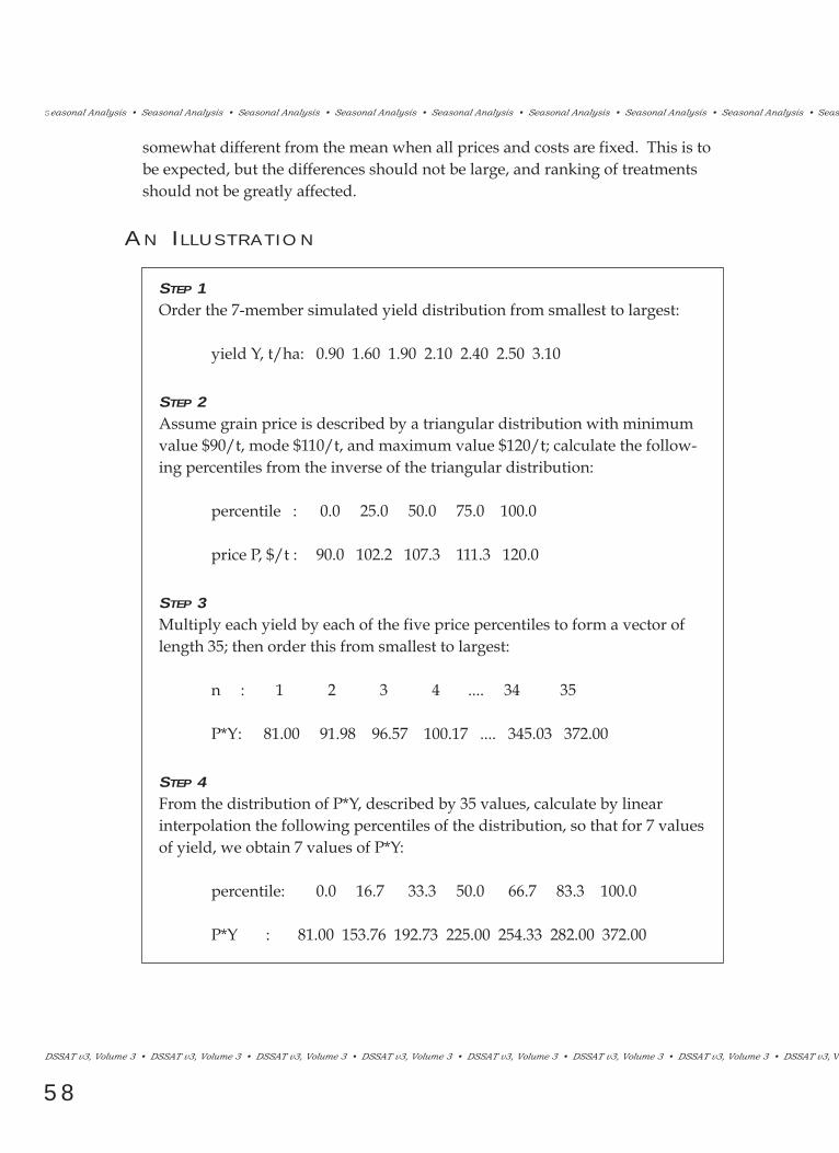
58
Seasonal Analysis ¥ Seasonal Analysis ¥ Seasonal Analysis ¥ Seasonal Analysis ¥ Seasonal Analysis ¥ Seasonal Analysis ¥ Seasonal Analysis ¥ Seasonal Analysis ¥ Seas
DSSAT v3, Volume 3 ¥ DSSAT v3, Volume 3 ¥ DSSAT v3, Volume 3 ¥ DSSAT v3, Volume 3 ¥ DSSAT v3, Volume 3 ¥ DSSAT v3, Volume 3 ¥ DSSAT v3, Volume 3 ¥ DSSAT v3, V
AN I L L U S T R AT I O N
somewhat different from the mean when all prices and costs are fixed. This is tobe expected, but the differences should not be large, and ranking of treatmentsshould not be greatly affected.
STEP 1Order the 7-member simulated yield distribution from smallest to largest:
yield Y, t/ha: 0.90 1.60 1.90 2.10 2.40 2.50 3.10
STEP 2 Assume grain price is described by a triangular distribution with minimumvalue $90/t, mode $110/t, and maximum value $120/t; calculate the follow-ing percentiles from the inverse of the triangular distribution:
percentile : 0.0 25.0 50.0 75.0 100.0
price P, $/t : 90.0 102.2 107.3 111.3 120.0
STEP 3Multiply each yield by each of the five price percentiles to form a vector oflength 35; then order this from smallest to largest:
n : 1 2 3 4 .... 34 35
P*Y: 81.00 91.98 96.57 100.17 .... 345.03 372.00
STEP 4From the distribution of P*Y, described by 35 values, calculate by linearinterpolation the following percentiles of the distribution, so that for 7 valuesof yield, we obtain 7 values of P*Y:
percentile: 0.0 16.7 33.3 50.0 66.7 83.3 100.0
P*Y : 81.00 153.76 192.73 225.00 254.33 282.00 372.00
59
• Analysis ¥ Seasonal Analysis ¥ Seasonal Analysis ¥ Seasonal Analysis ¥ Seasonal Analysis ¥ Seasonal Analysis ¥ Seasonal Analysis ¥ Seasonal Analysis ¥ Seasonal Analysis ¥
3 ¥ DSSAT v3, Volume 3 ¥ DSSAT v3, Volume 3 ¥ DSSAT v3, Volume 3 ¥ DSSAT v3, Volume 3 ¥ DSSAT v3, Volume 3 ¥ DSSAT v3, Volume 3 ¥ DSSAT v3, Volume 3 ¥ DSSAT v3,
sis
APPENDIX B.THREE DECISION CRITERIA
The stochastic efficiency rules are an important class of decision criteria, and areparticularly suited to the analysis of simulation model output. These have theirbasis in Bernoullian utility theory, and differ in the assumptions that are madeabout the decision makerÕs attitude to risk. (Refer to the ÒReferenceÓ section inthis Part for sources of information on the issues discussed in this appendix).These rules were developed to tackle the problem of portfolio selection in invest-ment theory, but are now firmly- entrenched tools for risk analysis in all sorts ofapplications. All involve a pair-wise comparison of random variables, and strict-ly speaking, these should relate to financial gains and losses. The result of theanalysis is an efficient set of treatments. The efficient set contains a subset oftreatments that are superior (there may be one only, but sometimes there will bemore than one efficient treatment). Three variations are described briefly below.
ME A N -VA R I A N C E (EV) AN A LY S I S
For two risky prospects, A and B, with means E(.) and variances V(.) respectively,then A dominates B if
E(A) = E(B) and V(A) < V(B) or ifV(A) = V(B) and E(A) > E(B).
A is then said to be EV-efficient. If prospects are plotted in EV space (V the ordi-nate, E the abscissa), then utility increases in a north-westerly direction. EVanalysis assumes that the decision maker has a quadratic utility function for gainsand losses, and/or that the risky prospects are distributed normally (or at leastdistributed symmetrically). These are often untenable assumptions, and the EVcriterion has fairly weak discriminatory power (i.e., the efficient sets tend to belarge).
ST O C H A S T I C DO M I N A N C E (SD) AN A LY S I S
For two risky prospects, A and B, A dominates B by first-order stochastic domi-nance (FSD) if the Cumulative Distribution Function (CDF) of gains from A lies tothe right of the CDF of B over the entire probability interval 0 to 1.
If the CDFs of A and B intersect, then no dominance by FSD can be established.

60
Seasonal Analysis ¥ Seasonal Analysis ¥ Seasonal Analysis ¥ Seasonal Analysis ¥ Seasonal Analysis ¥ Seasonal Analysis ¥ Seasonal Analysis ¥ Seasonal Analysis ¥ Seas
DSSAT v3, Volume 3 ¥ DSSAT v3, Volume 3 ¥ DSSAT v3, Volume 3 ¥ DSSAT v3, Volume 3 ¥ DSSAT v3, Volume 3 ¥ DSSAT v3, Volume 3 ¥ DSSAT v3, Volume 3 ¥ DSSAT v3, V
If, however, the area between the two CDFs below the point of intersection isgreater than the area between the two CDFs above the point of intersection, thenA dominates B by second-order stochastic dominance (SSD); otherwise, no domi-nance can be established, and both A and B are second-order efficient.
For FSD, no assumptions are made about the attitude of the decision maker torisk; for SSD, it is assumed the decision maker is averse to risk to some unknowndegree. No assumptions need be made about the distributional properties of therandom variables, either.
ME A N -G I N I DO M I N A N C E (MGD) AN A LY S I S
For two risky prospects, A and B, A dominates B by MGD if:
E(A) >= E(B) and E(A) - G(A) >= E(B) - G(B)
with strict inequality for one of these expressions, where E(.) is the mean, and G(.)is the Gini coefficient of distributions A and B (which is half the value of GiniÕsmean difference: the absolute expected difference of a pair of randomly selectedvalues of the variable).
MGD, like SSD, assumes that the decision maker is averse to risk, but unlike SSD,the extremely risk-averse are excluded from the analysis. It is thus a more dis-criminating decision rule than SSD (since the MGD efficient set is usually small-er), and computationally, MGD is generally much easier to establish than SSD.
AN EX A M P L E
In the seasonal analysis program, E-V analysis can be carried out visually from E-V plots of economic returns, and mean-Gini analysis may be carried out bychoosing the appropriate menu options. (Notes on first- and second-degree sto-chastic dominance are included for interestÕs sake for those readers familiar withDSSAT Version 2.1).
To illustrate, consider again the example obtained by analyzing the fileUFGA7812.SNS using the costs and prices as in the distribution version ofUFGA7812.PRI.
The box plot in Screen 24 (on following page) shows the impact of large amountsof irrigation on monetary returns per hectare. If you look at the amount of irriga-tion water applied in the six treatments (Screen 25, on 2nd following page) andcompare this with the yields obtained (see Screen 9), it is clear that much of the

61
• Analysis ¥ Seasonal Analysis ¥ Seasonal Analysis ¥ Seasonal Analysis ¥ Seasonal Analysis ¥ Seasonal Analysis ¥ Seasonal Analysis ¥ Seasonal Analysis ¥ Seasonal Analysis ¥
3 ¥ DSSAT v3, Volume 3 ¥ DSSAT v3, Volume 3 ¥ DSSAT v3, Volume 3 ¥ DSSAT v3, Volume 3 ¥ DSSAT v3, Volume 3 ¥ DSSAT v3, Volume 3 ¥ DSSAT v3, Volume 3 ¥ DSSAT v3,
sis
ALL_TRTS
BOX PLOT OF MONETARY RETURNS PER HA
1.080k
0.900k
0.720k
0.540k
0.360k
0.180k
MONEY / HA
TREATMENT
❈
❈
❈
❈
❈
❈
1 2 3 4 5 60 7
SCREEN 24.
water applied in Treatments 2, 3, and 4 is wasted; only a small amount ofsupplemental irrigation is required to alleviate most of the water stressthat may occur in most years.
The same can be seen in terms of the number of irrigation applicationsmade in each treatment (Screen 26, on following page). We can concludethat the cost of irrigation water per mm, the cost of each irrigation appli-cation, and the limited yield response to heavy irrigation applications,combine in such a way that the most profitable option of the six consid-ered is to apply irrigation at a threshold of 30 percent of field capacity.
1 2 3 4 5 6
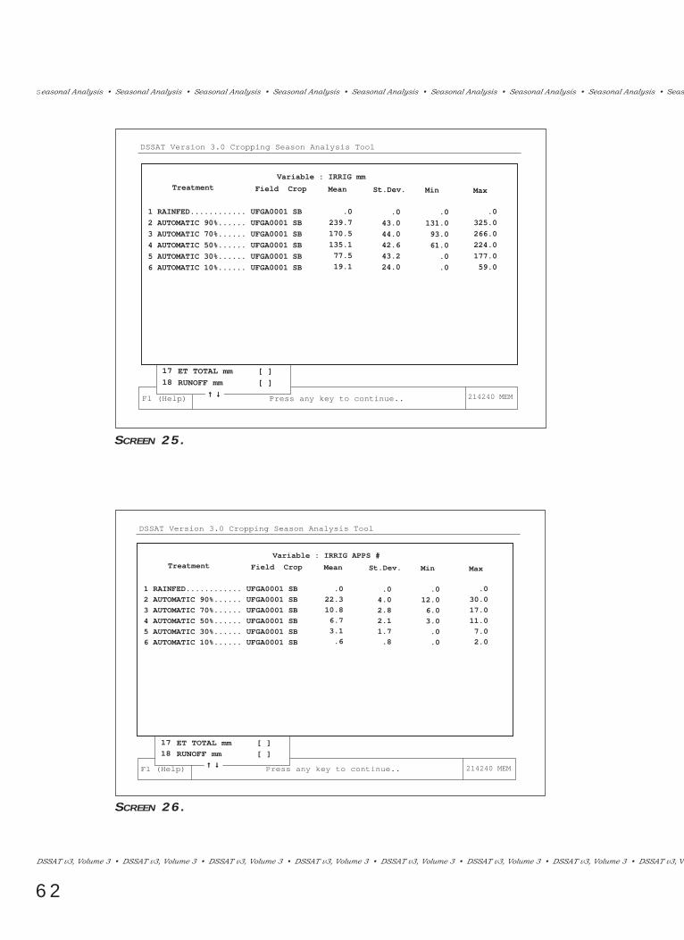
Select a cropping season file for analysis
Analyse Biological variables
Analyse Economic variables
Modify hardopy options
About VARAN2....
Exit
F1 (Help) 214240 Mem
Main Menu
DSSAT Version 3.0 Cropping Season Analysis Tool
Analysis1
2
3
4
5
6
7
8
9
10
11
12
13
14
15
16
17
18
START SIM day [ ]
PLANTING day [ ]
ANTHESIS day [ ]
MATURITY day [ ]
HARVET day [ ]
SOWING WT kg/ha [ ]
TOPS WT. kg/ha [ ]
MAT YIELD kg/ha [ ]
HAR YIELD kg/ha [ ]
BYPRODUCT kg/ha [ ]
WEIGHT mg/unit [ ]
NUMBER #/m2 [ ]
NUMBER #/unit [ ]
IRRIG APPS # [ ]
IRRIG mm [ ]
PRECIP mm [ ]
ET TOTAL mm [ ]
RUNOFF mm [ ]
↑ ↓
Variable : IRRIG mm
Treatment Field Crop Mean St.Dev. Min Max
1 RAINFED............ UFGA0001 SB
2 AUTOMATIC 90%...... UFGA0001 SB
3 AUTOMATIC 70%...... UFGA0001 SB
4 AUTOMATIC 50%...... UFGA0001 SB
5 AUTOMATIC 30%...... UFGA0001 SB
6 AUTOMATIC 10%...... UFGA0001 SB
.0
239.7
170.5
135.1
77.5
19.1
.0
43.0
44.0
42.6
43.2
24.0
.0
131.0
93.0
61.0
.0
.0
.0
325.0
266.0
224.0
177.0
59.0
Press any key to continue..
62
Seasonal Analysis ¥ Seasonal Analysis ¥ Seasonal Analysis ¥ Seasonal Analysis ¥ Seasonal Analysis ¥ Seasonal Analysis ¥ Seasonal Analysis ¥ Seasonal Analysis ¥ Seas
DSSAT v3, Volume 3 ¥ DSSAT v3, Volume 3 ¥ DSSAT v3, Volume 3 ¥ DSSAT v3, Volume 3 ¥ DSSAT v3, Volume 3 ¥ DSSAT v3, Volume 3 ¥ DSSAT v3, Volume 3 ¥ DSSAT v3, V
SCREEN 26.
SCREEN 25.
214240 MEM
Select a cropping season file for analysis
Analyse Biological variables
Analyse Economic variables
Modify hardopy options
About VARAN2....
Exit
F1 (Help) 204240 Mem
Main Menu
DSSAT Version 3.0 Cropping Season Analysis Tool
Analysis1
2
3
4
5
6
7
8
9
10
11
12
13
14
15
16
17
18
START SIM day [ ]
PLANTING day [ ]
ANTHESIS day [ ]
MATURITY day [ ]
HARVET day [ ]
SOWING WT kg/ha [ ]
TOPS WT. kg/ha [ ]
MAT YIELD kg/ha [ ]
HAR YIELD kg/ha [ ]
BYPRODUCT kg/ha [ ]
WEIGHT mg/unit [ ]
NUMBER #/m2 [ ]
NUMBER #/unit [ ]
IRRIG APPS # [ ]
IRRIG mm [ ]
PRECIP mm [ ]
ET TOTAL mm [ ]
RUNOFF mm [ ]
↑ ↓ Press any key to continue..
Variable : IRRIG APPS #
Treatment Field Crop Mean St.Dev. Min Max
1 RAINFED............ UFGA0001 SB
2 AUTOMATIC 90%...... UFGA0001 SB
3 AUTOMATIC 70%...... UFGA0001 SB
4 AUTOMATIC 50%...... UFGA0001 SB
5 AUTOMATIC 30%...... UFGA0001 SB
6 AUTOMATIC 10%...... UFGA0001 SB
.0
22.3
10.8
6.7
3.1
.6
.0
4.0
2.8
2.1
1.7
.8
.0
12.0
6.0
3.0
.0
.0
.0
30.0
17.0
11.0
7.0
2.0
214240 MEM

63
• Analysis ¥ Seasonal Analysis ¥ Seasonal Analysis ¥ Seasonal Analysis ¥ Seasonal Analysis ¥ Seasonal Analysis ¥ Seasonal Analysis ¥ Seasonal Analysis ¥ Seasonal Analysis ¥
3 ¥ DSSAT v3, Volume 3 ¥ DSSAT v3, Volume 3 ¥ DSSAT v3, Volume 3 ¥ DSSAT v3, Volume 3 ¥ DSSAT v3, Volume 3 ¥ DSSAT v3, Volume 3 ¥ DSSAT v3, Volume 3 ¥ DSSAT v3,
sis
700.0
600.0
500.0
400.0
MEAN, MONEY / HA
E-V PLOT OF MONETARY RETURNS PER HA
5
6
1
4
3
2
0.00K 10.00K 20.00K 30.00K 40.00K 50.00K 60.00K
VARIANCE, MONEY / HA
(1) ALL_TRTS
SCREEN 27.
In terms of strategy analysis, the mean-Gini dominance calculations are shown inScreen 22 of the main text. As noted above, the dominant strategy also has thehighest mean monetary return. In mean-Gini dominance, this will always be thecase, but it will sometimes happen that the variability associated with this Òhigh-meanÓ treatment will be so great that it will be joined in the efficient set by anoth-er treatment with lower mean but lower variability. In such a case, no decisioncan be made with respect to which of the efficient treatments is better withoutknowing more about the preferences and attitudes of the particular decisionmaker. In any case, you should always remember that there is a variety of

64
Seasonal Analysis ¥ Seasonal Analysis ¥ Seasonal Analysis ¥ Seasonal Analysis ¥ Seasonal Analysis ¥ Seasonal Analysis ¥ Seasonal Analysis ¥ Seasonal Analysis ¥ Seas
DSSAT v3, Volume 3 ¥ DSSAT v3, Volume 3 ¥ DSSAT v3, Volume 3 ¥ DSSAT v3, Volume 3 ¥ DSSAT v3, Volume 3 ¥ DSSAT v3, Volume 3 ¥ DSSAT v3, Volume 3 ¥ DSSAT v3, V
sources of error in simulation experiments: errors in input data and errors inmodel specification, to name but two. Treatments with similar economic (or evenbiological performance) are likely to be Òstatistically indistinguishableÓ in termsof the modelÕs inherent errors, in any case; there is then little point in applyingincreasingly sensitive analytical procedures in an attempt to distinguish what isprobably indistinguishable.
Visual inspection of the six treatments for mean-variance dominance can be donefor this experiment (see Screen 27, on previous page). Treatment 5 has the highestmean, but note from Screen 19 of the main text that the standard deviation (andhence the variance) of Treatments 4 and 5 are lower than that for Treatment 5.According to strict application of the E-V rules, Treatments 5, 4, and 3 are E-V effi-cient. The differences in simulated variances are very small between these threetreatments, however. You should be careful not to be dogmatic in interpretation,and bear in mind the errors in the model and the model input data.
For purposes of comparison, inspection of the CPF plot of monetary returns forthe six treatments (Screen 28, on following page) shows that none of the treat-ments is dominant by first-order stochastic dominance, since the CPF forTreatment 5 crosses the CPFs of Treatments 1 and 6. Further analysis (outside theDSSAT v3) shows that Treatment 5 is efficient or dominant according to second-order stochastic dominance.
As might be expected, the efficient sets of treatments according to the various sto-chastic efficiency rules are related (see Buccola and Subaei (1984) for moredetails). In essence, MG-efficient treatments and FSD/SSD efficient treatmentsare members of the EV-efficient set; further, MG efficient treatments are membersof the FSD/SSD efficient set. To put it another way, EV-efficient sets tend to belarger than FSD/SSD efficient sets, which in turn tend to be larger than MG-effi-cient sets.
One more point to bear in mind is that for comparison purposes, calculations aremade, and the analysis is carried out, on a per hectare basis. While making forsimplicity, this implies even more about the particular nature of the decision mak-erÕs attitudes and preferences, but is often forgotten or ignored. Strictly speaking,these types of decision analysis relate to gains and losses of money in relation tototal wealth. For further details, consult Raiffa (1968).

65
• Analysis ¥ Seasonal Analysis ¥ Seasonal Analysis ¥ Seasonal Analysis ¥ Seasonal Analysis ¥ Seasonal Analysis ¥ Seasonal Analysis ¥ Seasonal Analysis ¥ Seasonal Analysis ¥
3 ¥ DSSAT v3, Volume 3 ¥ DSSAT v3, Volume 3 ¥ DSSAT v3, Volume 3 ¥ DSSAT v3, Volume 3 ¥ DSSAT v3, Volume 3 ¥ DSSAT v3, Volume 3 ¥ DSSAT v3, Volume 3 ¥ DSSAT v3,
sis
SCREEN 28.
(1) TRT1(1) TRT3(1) TRT5
(1) TRT2(1) TRT4(1) TRT6
1.000
0.800
0.600
0.400
0.200
CUMULATIVE PROBABILITY
CPR PLOT OF MONETARY RETURNS PER HA
0.000k 0.180k 0.360k 0.540k 0.720k 0.900k 1.080k
MONEY / HA
TRT6
TRT2TRT3
TRT4
TRT1
TRT5

66
Seasonal Analysis ¥ Seasonal Analysis ¥ Seasonal Analysis ¥ Seasonal Analysis ¥ Seasonal Analysis ¥ Seasonal Analysis ¥ Seasonal Analysis ¥ Seasonal Analysis ¥ Seas
DSSAT v3, Volume 3 ¥ DSSAT v3, Volume 3 ¥ DSSAT v3, Volume 3 ¥ DSSAT v3, Volume 3 ¥ DSSAT v3, Volume 3 ¥ DSSAT v3, Volume 3 ¥ DSSAT v3, Volume 3 ¥ DSSAT v3, V

P.K. THORNTON,P.W. WILKENS, G. HOOGENBOOM, J.W. JONES
VO L U M E 3 -2
SEQUENCEANALYSIS
INTERNATIONAL FERTILIZER DEVELOPMENT CENTER
UNIVERSITY OF FLORIDA, UNIVERSITY OF GEORGIA
INTERNATIONAL BENCHMARK SITES NETWORK FOR AGROTECHNOLOGY TRANSFER

Sequence Analysis ¥ Sequence Analysis ¥ Sequence Analysis ¥ Sequence Analysis ¥ Sequence Analysis ¥ Sequence Analysis ¥ Sequence Analysis ¥
DSSAT v3, Volume 3 ¥ DSSAT v3, Volume 3 ¥ DSSAT v3, Volume 3 ¥ DSSAT v3, Volume 3 ¥ DSSAT v3, Volume 3 ¥ DSSAT v3, Volume 3 ¥ DSSAT v3, V
68

equence Analysis ¥ Sequence Analysis ¥ Sequence Analysis ¥ Sequence Analysis ¥ Sequence Analysis ¥ Sequence Analysis ¥ Sequence Analysis ¥ Sequence
69
• DSSAT v3, Volume 2 • DSSAT v3, Volume 2 • DSSAT v3, Volume 2 • DSSAT v3, Volume 2 • DSSAT v3, Volume 2 • DSSAT v3, Volume 2 • DSSAT v3,
CHAPTER ONE.INTRODUCTION
The Sequence Analysis program allows the user to carry out simulations of croprotations or crop sequences (i.e., any combination of crops grown one after anoth-er) using the DSSAT v3 crop models, and then to analyze the results. A simulationexperiment involving a crop rotation may be replicated through time using differ-ent weather sequences; the experiment is set up by the user, the appropriate mod-els are run using a special program called the driver, and the user can then analyzethe results using the sequence analysis program. The ÒsequenceÓ aspect of the dri-ver and analysis programs relates to the fact that what is being run are experimentsof multiple cropping seasons; the carry-over of soil water and nutrient status iseffected from one season or crop to the subsequent season or crop.
To clarify the terminology, a number of definitions are set out below:
Sequence: relates to the growing of particular crops, one after another over time,where the carry-over effects from one crop to the next, whatever they may be, aretaken into account. A sequence may thus relate to the growing of maize plantedevery year for 10 years; a sequence may be a short rotation of maize planted everyseason followed by beans grown in the same wet season or calendar year; or asequence may consist of a four-year crop rotation, for example.
Treatment: any particular sequence run over a number of years; treatment 1 mightrefer to maize grown every year for 10 years with low exogenous nitrogen fertilizerinput; treatment 2 the same, with high nitrogen input; treatment 3, a maize-beancropping system in alternate seasons with low nitrogen input; and so on.
Replicate: a repetition of the same sequence treatment run over the same condi-tions apart from weather. In a real field experiment, two sequence replicates mightrefer to neighboring plots run with the same weather conditions, or the sequencesmight be replicated with respect to time: replicate 1 grown over the period 1981-1985, and replicate 2 from 1986 to 1990. In the same way that computer experi-mentation can produce ÒpureÓ replication of single season performance by usingmultiple year weather sequences, so computer experimentation can produce purereplication of sequences, where starting conditions and management are identical,but variation arises out of different weather sequences over the years of interestand out of any intrinsic stochasticity that may be built into the model.

Variation: for a simulation model with no intrinsic stochasticity (such as theCERES or CROPGRO models), the sources of variation in a computer experimentarise from the following: (a) between treatments; (b) between replicates; (c) withinsequences (i.e., between different years of the various sequence replicates). As forreplicated computer experiments run over single seasons, the only sources of errorthat exist are model error and input data error, ultimately, as opposed to fieldexperiments, where errors arise from measurement, micro-variations in soil andclimate, and the rest. This ÒpureÓ replication can be difficult to analyze and inter-pret in the case of cropping sequences.
The driver program is capable of running up to 10 ÒtreatmentsÓ or sequences. Theanalysis program, however, is capable of analyzing only one treatment at a time.Thus no direct treatment comparisons are possible using the analysis program.The major reason for this is to help foster Òhealthy skepticismÓ of sequence simula-tion results. At the current time, the sequence capabilities of the IBSNAT cropmodels have not been extensively tested. It is envisaged that most users of thesequence capability of the models will be interested in addressing Òwhat if...Óquestions related to agricultural system performance. However, analysis results ofmultiple treatment sequence experiments are written to an ASCII file, and you cananalyze these in any way you see fit outside the confines of DSSAT v3. You could,for example, compare and contrast different sequence strategies directly, althoughyou should exercise care in interpreting the results you obtain.
There are three basic steps involved in Sequence Analysis:
1. The creation of an appropriate model input file;2. Running the crop model(s) using the sequence driver;3. Analyzing the results of the simulations using the analysis program.
The links between these steps are shown in Figure 1. Sequence analyses are runfrom the DSSAT v3 Shell (see Volume 1-3, Hunt et al. 1994, of this book for adescription of the Shell) under the main menu item, ANALYSES. The three stepsare explained in Chapter 2 herein.
Sequence Analysis ¥ Sequence Analysis ¥ Sequence Analysis ¥ Sequence Analysis ¥ Sequence Analysis ¥ Sequence Analysis ¥ Sequence Analysis ¥
DSSAT v3, Volume 3 ¥ DSSAT v3, Volume 3 ¥ DSSAT v3, Volume 3 ¥ DSSAT v3, Volume 3 ¥ DSSAT v3, Volume 3 ¥ DSSAT v3, Volume 3 ¥ DSSAT v3, V
70
The useable portion of your systemÕs 640 Kb RAM should be at least 540 Kb in sizefor the models to run and for the analysis program and graphics to work.
If the driver or analysis program still does not work properly, one problem may be
SY S T E M RE Q U I R E M E N T S

equence Analysis ¥ Sequence Analysis ¥ Sequence Analysis ¥ Sequence Analysis ¥ Sequence Analysis ¥ Sequence Analysis ¥ Sequence Analysis ¥ Sequence
¥ DSSAT v3, Volume 3 ¥ DSSAT v3, Volume 3 ¥ DSSAT v3, Volume 3 ¥ DSSAT v3, Volume 3 ¥ DSSAT v3, Volume 3 ¥ DSSAT v3, Volume 3 ¥ DSSAT v3, Volume
71
FIGURE 1. STEPS IN SEQUENCE ANALYSIS.
associated with the number of BUFFERS and FILES defined in CONFIG.SYS.These will need to be set to at least 20 each.
Replicated sequence simulations on an 8086 or 80286 system may take a greatdeal of time. Sequence Analysis, like the rest of DSSAT v3, will operate without amath coprocessor, but this is not recommended.
DSSATPRO.FLE
XCREATEPROGRAM
OR
ASCIITEXT
EDITOR
EXP.LSTDRIVER
PROGRAM
EBAF1101.SQX
UFGA7801.SQX
FILEXs
CROP
MODELS
OUTPUT FILES
SEQUENCE.LST
SUMMARYOUTPUT
FILES
STEP 1 CREATE A FILEX
STEP 2 RUN THE EXPERIMENT
DSSATPRO.FLE
PRICE FILE(S) *.PRQ
SEQUENCE
ANALYSIS
PROGRAMEBAF1101.SQR
ANALYSISRESULTS
FILES
STEP 3 ANALYZE MODEL OUTPUTS
FILEX are crop model input files, listed in EXP.LST
Summary Output Files contain model outputs, and are listed in SEQUENCE.LST
ANALYSIS RESULTS FILES contain the results of all analyses carried out
DSSATPRO.FLE contains path information for all components of the DSSAT v3
PRICE FILES for sequence analysis have the extension PRQ
NOTES
EBAF1101.SQS

Sequence Analysis ¥ Sequence Analysis ¥ Sequence Analysis ¥ Sequence Analysis ¥ Sequence Analysis ¥ Sequence Analysis ¥ Sequence Analysis ¥
DSSAT v3, Volume 3 ¥ DSSAT v3, Volume 3 ¥ DSSAT v3, Volume 3 ¥ DSSAT v3, Volume 3 ¥ DSSAT v3, Volume 3 ¥ DSSAT v3, Volume 3 ¥ DSSAT v3, V
72

equence Analysis ¥ Sequence Analysis ¥ Sequence Analysis ¥ Sequence Analysis ¥ Sequence Analysis ¥ Sequence Analysis ¥ Sequence Analysis ¥ Sequence
¥ DSSAT v3, Volume 3 ¥ DSSAT v3, Volume 3 ¥ DSSAT v3, Volume 3 ¥ DSSAT v3, Volume 3 ¥ DSSAT v3, Volume 3 ¥ DSSAT v3, Volume 3 ¥ DSSAT v3, Volume
73
CHAPTER TWO.CREATING MODEL INPUT FILES FOR
SEQUENCE ANALYSIS
F I LEX FO R SE Q U E N C E AN A LY S I S
The utility program XCreate that is provided with the DSSAT v3 software can beused to create model input files for running sequence analyses (see Volume 1-4,Imamura 1994, of this book for a description of the XCreate program). Thesemodel input files are referred to as FILEXs (see Volume 2-1, Jones et al. 1994, ofthis book for a description of this file). Alternatively, these files can be createdusing an ASCII text editor. The advantage of using the program XCreate is thatthe experiment listing file EXP.LST (see Volume 2-1, Jones et al. 1994, of this bookfor a description of this file) is updated automatically. If you create a sequenceanalysis FILEX yourself, you must either update EXP.LST or run the FileManager Utility program (accessed using the ÒSequence Ñ InputsÓ menu itemsof the DSSAT v3 Shell; see Volume 1-3, Hunt et al. 1994, of this book for a descrip-tion of the Shell) for the FILEX to be accessible to the system. The format ofEXP.LST is shown in Table 1.
Sequence analysis model input files created with XCreate have the extensionSQX. An example of a sequence analysis FILEX is shown in Table 2. There aresome important differences in the way in which a sequencing FILEX is set up,compared with experiment or seasonal FILEXs. In the *TREATMENTS section ofthe file, instead of setting up a number of treatments, you specify a rotationÒgermÓ; this is the sequence of crops that will be repeated over and over again.In Table 2, for instance, the ÒgermÓ consists of maize, followed by fallow (i.e., nocrop is planted, but the models will simulate the soil water and nutrient processeson a daily basis until the next crop is planted). Note that the treatment number
TABLE 1. SEQUENCE EXPERIMENT LISTING FILE EXP.LST.
*EXPERIMENT LIST
@# FILENAME EXT ENAME
1 UFGA7803 SQX SEQUENCE ANALYSIS, SIMPLE MULTI-TREAT FILE, 5:5
2 UFGA7804 SQX BN-BN YR 1, SB YR 2 EXAMPLE, 10:5
3 EBAF1101 SQX MA-FA, 30 YRS, 15 REPS, NO N

Sequence Analysis ¥ Sequence Analysis ¥ Sequence Analysis ¥ Sequence Analysis ¥ Sequence Analysis ¥ Sequence Analysis ¥ Sequence Analysis ¥
DSSAT v3, Volume 3 ¥ DSSAT v3, Volume 3 ¥ DSSAT v3, Volume 3 ¥ DSSAT v3, Volume 3 ¥ DSSAT v3, Volume 3 ¥ DSSAT v3, Volume 3 ¥ DSSAT v3, V
74
(@N) is 1 for both rotation components. Each rotation component is assigned anumber in ascending order, starting from 1 (the R column). Thus maize is the firstcomponent (R = Ò1Ó), and fallow is the second (R = Ò2Ó). The variables O and C insequencing FILEXs should always be set to Ò1Ó and Ò0,Ó respectively. These areoptions that have not yet been implemented.
The rotation germ will be repeated for as many seasons as are specified in the*SIMULATION CONTROLS section of the FILEX, under NYERS (one of the GEN-ERAL options found in this section). In Table 2, NYERS is Ò30,Ó so the rotationwill be continued for 30 years.
This example FILEX specifies that maize is to be planted on day 305 (from PDATEin the *PLANTING DETAILS section of the file; note that PLANT under MAN-AGEMENT options in the *SIMULATION CONTROLS block 1 (i.e., N =Ó1Ó) is setto ÒRÓ for ÒrecordedÓ) in each year of simulation. Once the maize is mature, thefallow model will be run, until the maize model is called for planting in the nextyear.
This FILEX also specifies that there are to be 15 replicates of this sequence (refer toNREPS under GENERAL options in *SIMULATION CONTROLS block 1).Weather for the site EBAF is to be simulated using WGEN (refer to WTHER underthe METHOD options in *SIMULATION CONTROLS block 1; this is set to ÒWÓ).
You will notice that there are two simulation control blocks in this FILEX. In gen-eral, it is highly recommended that you specify as many simulation control blocksas there are rotation components. So if you specify 7 rotation components, it issafest to specify 7 simulation control blocks.
For sequence experiments, you should note that the values of NYERS, NREPS,START, YRDAY, RSEED, all the OPTIONS variables, WTHER, and all the OUT-PUTS variables are taken from the *SIMULATION CONTROLS block with thelowest VALID number. The values of these variables in any other *SIMULATIONCONTROLS block are ignored. Thus in Table 2, the random number seed RSEED,for example, in block 1 equals 3517; in block 2, RSEED equals 2150. Since block 1 isa valid block number (i.e., in the *TREATMENTS section SM is specified as Ò1Ó forthe first component), then the values appearing here will be used. Block 2 is alsovalid, but the values of NYERS, etc., will be ignored. In general, you may specifysimulation controls as you would for experiment or seasonal FILEXs; thus youmay specify automatic planting, etc.

equence Analysis ¥ Sequence Analysis ¥ Sequence Analysis ¥ Sequence Analysis ¥ Sequence Analysis ¥ Sequence Analysis ¥ Sequence Analysis ¥ Sequence
¥ DSSAT v3, Volume 3 ¥ DSSAT v3, Volume 3 ¥ DSSAT v3, Volume 3 ¥ DSSAT v3, Volume 3 ¥ DSSAT v3, Volume 3 ¥ DSSAT v3, Volume 3 ¥ DSSAT v3, Volume
75
TABLE 2. A SAMPLE FILEX FOR CROP SEQUENCING: EBAF1101.SQX.
*EXP.DETAILS: EBAF1101SQ MAIZE-FALLOW, 30 YEARS, 15 REPS, NO N
*TREATMENTS ———-FACTOR LEVELS———@N R O C TNAME.................... CU FL SA IC MP MI MF MR MC MT ME MH SM1 1 1 0 Maize component 1 1 0 1 1 0 0 1 0 0 0 0 11 2 1 0 Fallow component 2 2 0 0 0 0 0 0 0 0 0 1 2
*CULTIVARS@C CR INGENO CNAME1 MZ IB0058 NC+592 FA IB0001
*FIELDS@L ID_FIELD WSTA.... FLSA FLOB FLDT FLDD FLDS FLST SLTX SLDP IB_SOIL1 EBAF0001 EBAF -99 0 IB000 0 0 00000 -99 180 IBMZ910032
*INITIAL CONDITIONS@C PCR ICDAT ICRT ICND ICRN ICRE1 MZ 11244 100 -99 1.00 1.00@C ICBL SH20 SNH4 SNO31 5 0.265 0.6 1.51 10 0.265 0.6 1.51 20 0.265 0.6 1.51 30 0.248 0.6 1.51 40 0.248 0.6 1.51 50 0.248 0.6 1.51 60 0.248 0.6 1.51 70 0.248 0.6 1.51 80 0.248 0.6 1.51 100 0.248 0.6 1.01 120 0.248 0.6 1.0
*PLANTING DETAILS@P PDATE EDATE PPOP PPOE PLME PLDS PLRS PLRD PLDP PLWT PAGE PENV PLPH1 11305 -99 6.2 6.2 S R 80 0 5.0 -99 -99 -99.0 -99.0
*RESIDUES AND OTHER ORGANIC MATERIALS@R RDATE RCOD RAMT RESN RESP RESK RINP RDEP1 11300 IB001 5000 0.8 -9 -9 15
*HARVEST DETAILS@R HDATE HSTG HCOM HSIZ HPC1 12304 100.0
*SIMULATION CONTROLS@N GENERAL NYERS NREPS START YRDAY RSEED SNAME....................1 GE 30 15 S 11244 3517 MZ component@N OPTIONS WATER NITRO SYMBI PHOSP POTAS DISES1 OP Y Y Y N N N

Sequence Analysis ¥ Sequence Analysis ¥ Sequence Analysis ¥ Sequence Analysis ¥ Sequence Analysis ¥ Sequence Analysis ¥ Sequence Analysis ¥
DSSAT v3, Volume 3 ¥ DSSAT v3, Volume 3 ¥ DSSAT v3, Volume 3 ¥ DSSAT v3, Volume 3 ¥ DSSAT v3, Volume 3 ¥ DSSAT v3, Volume 3 ¥ DSSAT v3, V
76
@N METHODS WTHER INCON LIGHT EVAPO INFIL PHOTO1 ME W M E R S C@N MANAGEMENT PLANT IRRIG FERTI RESID HARVS1 MA R N R R M@N OUTPUTS FNAME OVVEW SUMRY FROPT GROTH CARBN WATER NITRO MINER DISES LONG1 OU Y N A 7 N N N N N N N
@ AUTOMATIC MANAGEMENT@N PLANTING PFIRST PLAST PH2OL PH2OU PH2OD PSTMX PSTMN1 PL 288 360 40 100 30 40 10@N IRRIGATION IMDEP ITHRL ITHRU IROFF IMETH IRAMT IREFF1 IR 30 50 100 IB001 IB001 10 0.75@N NITROGEN NMDEP NMTHR NAMNT NCODE NAOFF1 NI 30 50 25 IB001 IB001@N RESIDUES RIPCN RTIME RIDEP1 RE 100 1 20@N HARVEST HFIRST HLAST HPCNP HPCNR1 HA 0 365 100 0
@N GENERAL NYERS NREPS START YRDAY RSEED SNAME....................2 GE 30 15 S 11244 2150 FA component@N OPTIONS WATER NITRO SYMBI PHOSP POTAS DISES2 OP Y Y Y N N N@N METHODS WTHER INCON LIGHT EVAPO INFIL PHOTO2 ME W M E R S C@N MANAGEMENT PLANT IRRIG FERTI RESID HARVS2 MA R N R R R@N OUTPUTS FNAME OVVEW SUMRY FROPT GROTH CARBN WATER NITRO MINER DISES LONG2 OU Y N A 7 N N N N N N N
@ AUTOMATIC MANAGEMENT@N PLANTING PFIRST PLAST PH2OL PH2OU PH2OD PSTMX PSTMN2 PL 155 200 40 100 30 40 10@N IRRIGATION IMDEP ITHRL ITHRU IROFF IMETH IRAMT IREFF2 IR 30 50 100 IB001 IB001 10 0.75@N NITROGEN NMDEP NMTHR NAMNT NCODE NAOFF2 NI 30 50 25 IB001 IB001@N RESIDUES RIPCN RTIME RIDEP2 RE 100 1 20@N HARVEST HFIRST HLAST HPCNP HPCNR2 HA 0 365 100 0

equence Analysis ¥ Sequence Analysis ¥ Sequence Analysis ¥ Sequence Analysis ¥ Sequence Analysis ¥ Sequence Analysis ¥ Sequence Analysis ¥ Sequence
¥ DSSAT v3, Volume 3 ¥ DSSAT v3, Volume 3 ¥ DSSAT v3, Volume 3 ¥ DSSAT v3, Volume 3 ¥ DSSAT v3, Volume 3 ¥ DSSAT v3, Volume 3 ¥ DSSAT v3, Volume
77
Refer to the *TREATMENTS section in Table 2. Factor levels are specified as forexperiment or seasonal FILEXs. Thus, we have to specify a cultivar level (CU) foreach rotation component (even fallow, although this is a dummy value). Therotation is grown in the same plot of land (FL = Ó1Ó for both rotation compo-nents). Initial conditions (IC) are specified for the maize component (IC = Ó1;Ónote that these are the conditions that will pertain at the start of each sequence; insubsequent seasons, Òinitial conditionsÓ in terms of soil water and ammoniumand nitrate levels are output by the preceding fallow model). Planting of maizetakes place according to the *PLANTING DETAILS section 1 (MP = Ó1Ó formaize). Crop residue is applied at the start of the sequence according to the val-ues specified in *RESIDUES section 1 (MR = Ó1Ó). The maize crop is controlledby the simulation controls in SM=Ó1.Ó
For the fallow component, the cultivar and field is specified (CU = Ó2Ó and FL =Ó1Ó). Simulation control is specified (SM= Ó2,Ó see above). One further factorlevel is needed: a *HARVEST DETAILS section (MH = Ò1Ó) is REQUIRED for anyfallow component. This is necessary to tell the fallow model when to stop. In theHDATE slot (harvest date) found in the *HARVEST DETAILS section, you mustspecify a year and date for the fallow model to halt. This must be specified sothat it precedes the planting date, PDATE, of the next crop found in the *PLANT-ING DETAILS section, if planting is done as recorded (i.e., if PLANT = ÒR,Ó as itdoes in Table 2 in the *SIMULATION CONTROLS section for the maize crop). Ifplanting should be automatic (PLANT = ÒAÓ), then you should specify a value ofHDATE such that it precedes or is equal to the first date of the planting windowfor the next crop; this would be specified in PFIRST in the AUTOMATIC MAN-AGEMENT section of the relevant *SIMULATION CONTROLS block.
Note that in Table 2, HDATE is set to 12304. The year must be set to 12, since themaize is first planted in 1911 (i.e. we have to look ahead to the next maize crop),and day 304 precedes the planting date PDATE of 305.
Remember that this is a hypothetical sequence simulation; years have to be speci-fied, and the FILEX in Table 2 assumes that the crop is planted in 1911. The actu-al year that the simulation starts is up to the user, since simulated weather is to beused.
Note that you could specify a year of fallow in the experiment simply by settingHDATE to 13304.

Sequence Analysis ¥ Sequence Analysis ¥ Sequence Analysis ¥ Sequence Analysis ¥ Sequence Analysis ¥ Sequence Analysis ¥ Sequence Analysis ¥
DSSAT v3, Volume 3 ¥ DSSAT v3, Volume 3 ¥ DSSAT v3, Volume 3 ¥ DSSAT v3, Volume 3 ¥ DSSAT v3, Volume 3 ¥ DSSAT v3, Volume 3 ¥ DSSAT v3, V
78
One of the most difficult things to define is the control of timing by the driverand the crop models when run in sequence. Time is controlled internally in themodels and the driver. All that is required from FILEX is that there is enoughinformation to specify what happens exactly for the first germ of the rotation. Insubsequent run-throughs of the germ, the years of planting, fertilizer additions,etc., will be automatically updated.
It is important that you understand how these operate for sequencing,becausesome users may want to set up sequence FILEXs manually. Some practice willprobably be needed in this. The table below may help to make things clearer; itshows the first few iterations of the sequence specified in Table 2:
Run Number Crop Started Finished Year Day Year Day
ÑÑÑÑÑÑÑÑÑÑÑÑÑÑÑÑÑÑÑÑÑÑÑÑÑÑÑÑÑ1 MZ 1911 244 1912 059 } germ 12 FA 1912 060 1912 304 } Ò3 MZ 1912 305 1913 057 } germ 24 FA 1913 058 1913 304 } Ò5 MZ 1913 305 1914 049 } germ 3etc.
ÑÑÑÑÑÑÑÑÑÑÑÑÑÑÑÑÑÑÑÑÑÑÑÑÑÑÑÑÑ
ÒStartedÓ refers to the date when the appropriate crop model was called; Òfin-ishedÓ refers to when the appropriate crop model ended its run. The maizemodel ÒfinishedÓ its run once maturity had been reached; this is dependent onweather, to some extent, so that it may vary from one year to the next. The fallowmodel thus started at different dates, but it finished on the same day each year, asspecified by HDATE. Note also that the starting date of simulation is day 244 of1911, specified by YRDAY in *SIMULATION CONTROLS block 1. Initial condi-tions relate to this date also (ICDAT = 11244 in the *INITIAL CONDITIONS sec-tion), and residue is added to the system on day 300 of 1911 (RDATE = 11300 inthe *RESIDUES section). Planting of maize, however, first takes place on day 305of 1911, and on day 305 of each year thereafter (PDATE = 11305 in the *PLANTI-NG DETAILS section).
T I M I N G CO N T R O L S

equence Analysis ¥ Sequence Analysis ¥ Sequence Analysis ¥ Sequence Analysis ¥ Sequence Analysis ¥ Sequence Analysis ¥ Sequence Analysis ¥ Sequence
¥ DSSAT v3, Volume 3 ¥ DSSAT v3, Volume 3 ¥ DSSAT v3, Volume 3 ¥ DSSAT v3, Volume 3 ¥ DSSAT v3, Volume 3 ¥ DSSAT v3, Volume 3 ¥ DSSAT v3, Volume
79
There are a number of simulation control options in FILEX that are generallyimportant for sequence analyses (refer to the *SIMULATION CONTROLS blocknumber 1 (i.e., N = 1) in Table 2). These are described as follows.
NYERSNYERS is the length of the sequence in years; it has a different meaning fromNYERS in Seasonal Analysis (refer to Part 1 of this Volume, Volume 3-1, Thorntonet al. 1994). NYERS may have a value between 1 and 50. Sequence experimentswill normally be run using simulated weather (i.e., where the variable WTHER,one of the METHOD options, is set to ÒWÓ or ÒSÓ). If you have a real long-termexperiment, this will presumably be unreplicated in terms of weather; you maythen use WTHER set to ÒMÓ (ÒmeasuredÓ weather). If for any reason you want torun a replicated sequence using historical weather, you would have to set up theFILEX to have multiple treatments with a different *FIELDS block for each repli-cate; you would specify the germ for each treatment, and specify a different histori-cal weather file to start the run with under the ÒWSTA....Ó header variable in each*FIELDS control block. You would then need to check the availability of historicalweather data files.
NREPSNREPS specifies the number of replicates of the rotation or crop sequence. It mayvary from 1 to 20. The impact of replication on the stability of simulation results isvery important, and is addressed in the Appendix to this Part.
CAUTION: You are highly recommended to read the Appendix before using any of thesequence capabilities of DSSAT v3; it is easy to produce misleading results from analysis ofsimulated sequence experiments.
RSEEDRSEED is the random number seed for weather generation. With the same seed,you will obtain the same sequence of random numbers, and hence the samesequence of daily weather, if you start from the same starting date of simulation(SDATE). RSEED is used only if WTHER is set to ÒWÓ or ÒS.Ó When sequences arereplicated, the initial RSEED used is incremented to Rnew from the value in FILEXaccording to:
Rnew = RSEED + 5(i-1)
S I M U L AT I O N CO N T R O L OP T I O N S

Sequence Analysis ¥ Sequence Analysis ¥ Sequence Analysis ¥ Sequence Analysis ¥ Sequence Analysis ¥ Sequence Analysis ¥ Sequence Analysis ¥
DSSAT v3, Volume 3 ¥ DSSAT v3, Volume 3 ¥ DSSAT v3, Volume 3 ¥ DSSAT v3, Volume 3 ¥ DSSAT v3, Volume 3 ¥ DSSAT v3, Volume 3 ¥ DSSAT v3, V
80
where i is the replicate number. If you run into problems, this will allow you to beable to calculate the value of the random number seed that gave rise to the problem,generate the offending weather sequence, and, hopefully, reproduce and isolate theproblem.
FNAMEIf this switch is set to ÒN,Ó then the summary output file from the model runs will benamed SUMMARY.SQS. If FNAME is set to ÒY,Ó then the summary output file namewill be the same as the model FILEX name, except that the last letter of the extensionwill be changed from X to S. Thus for the experiment FILEX in Table 2, which has thename EBAF1101.SQX, the summary output file will be named EBAF1101.SQS, sincethe switch FNAME is set to ÒY.Ó
SUMRYFor sequence simulations, this controller should always be set to A (append), other-wise the summary output file will be successively overwritten by each treatment andearlier outputs lost. In Table 2, all the other OUTPUTS options are set to ÒN,Ó to pre-vent output from the models. Since sequence simulations with many replicates canproduce prodigious quantities of output data, it makes sense to turn these output filesoff, unless you need them specifically.
Although setting up sequence FILEXs may seem complicated, it is rather flexible. Thedistribution diskette of the Sequence Analysis program contains two other sequenceFILEXs that illustrate some of this flexibility. UFGA7803.SQX contains a simple multi-ple treatment experiment. Treatment 1 involves soybean and fallow, and Treatment 2bean and fallow. Pay special attention to the values of N and R in the *TREATMENTSsection of this file.
Another FILEX that is distributed with the DSSAT v3 software is UFGA7804.SQX.This is a more complicated rotation involving two bean crops in one season followedby soybean in the next. The rotation germ is thus specified as BN1 - FA1 - BN2 - FA2 -SB1 - FA3, spanning two seasons. Each fallow is distinct and must be so treated in theanalysis (see Chapter 4 herein).
You may specify rotations with up to 9 distinct components. The sequence driver willoperate even if no fallows are specified between each crop component. However, youare highly recommended to specify fallows between each crop component. It is alsogenerally a good idea to make the sequence length exactly divisible by the germlength; thus, if your germ describes a four-year rotation, set NYERS to a multiple offour. This will avoid possible confusion when using the Sequence Analysis program.

equence Analysis ¥ Sequence Analysis ¥ Sequence Analysis ¥ Sequence Analysis ¥ Sequence Analysis ¥ Sequence Analysis ¥ Sequence Analysis ¥ Sequence
¥ DSSAT v3, Volume 3 ¥ DSSAT v3, Volume 3 ¥ DSSAT v3, Volume 3 ¥ DSSAT v3, Volume 3 ¥ DSSAT v3, Volume 3 ¥ DSSAT v3, Volume 3 ¥ DSSAT v3, Volume
81
CHAPTER THREE.RUNNING SEQUENCE ANALYSIS EXPERIMENTS
OV E RV I E W
The Sequence Analysis driver program takes the FILEX selected or created by theuser, and runs through the rotation germ until NYERS have elapsed, calling theappropriate crop model.
The driver is a FORTRAN program that allows the user to pick an entry fromEXP.LST (i.e., a particular FILEX; see Volume 2-1, Jones et al. 1994, of this book for adescription of the EXP.LST file). The FILEX is then read and various controls areset. Each rotation component specified in the FILEX is then run in its order ofappearance in the *TREATMENTS block of the FILEX. The appropriate model iscalled for each component (the model is run under the command of the driver pro-gram), and it will be run for as many years as are specified by NYERS and for asmany replicates as are specified by NREPS in the FILEX. When all runs have beencompleted, the results listing file SEQUENCE.LST (see the example in Table 3) isupdated with the name and description of the summary output file produced. Theuser can then quit the program or choose another FILEX for running under thesequence driver.
The sequence driver can be run in a stand-alone mode or through the DSSAT v3Shell (Volume 1-3, Hunt et al.1994, of this book). It is important to note that inwhich ever mode the driver is run, the program expects to find the model pro-gram(s) in the same directory. If model executable files are not found in that direc-tory, then an error message is printed and the user must arrange the executablefiles so that this condition is met. The file DSSATPRO.FLE (see the Appendix toVolume 1 of this book for a description of this file) also expected to be in this samedirectory, with appropriate pointers to the relevant directories for the crop modelexecutable files.
TABLE 3. SUMMARY MODEL OUTPUT LISTING FILE SEQUENCE.LST.
*SEQUENCING LIST
@# FILENAME EXT ENAME
1 UFGA7803 SQS SEQUENCE ANALYSIS, SIMPLE MULTI-TREAT FILE, 5:52 UFGA7804 SQS BN-BN YR 1, SB YR 2 EXAMPLE, 10:53 EBAF1101 SQS MZ-FA, 30 YRS, 15 REPS, NO N

Sequence Analysis ¥ Sequence Analysis ¥ Sequence Analysis ¥ Sequence Analysis ¥ Sequence Analysis ¥ Sequence Analysis ¥ Sequence Analysis ¥
DSSAT v3, Volume 3 ¥ DSSAT v3, Volume 3 ¥ DSSAT v3, Volume 3 ¥ DSSAT v3, Volume 3 ¥ DSSAT v3, Volume 3 ¥ DSSAT v3, Volume 3 ¥ DSSAT v3, V
82
On activating the ÒSimulateÓ option under the ÒSequenceÓ window (Screen 1,below), the driver program is activated, and the user is presented with Screen 2(on following page). Screen 2 contains the contents of the file EXP.LST, the listingfile in the current directory of current or selected FILEXs for sequence analysis.This lists the file number, file name, crop group code (ÒSQÓ for sequence analy-sis), and description. The description may be up to 60 characters long; if it isshorter, the description is padded with full stops. The file description is obtainedfrom columns 26 through 85 of the first line of FILEX (see Table 2).
If the colors on the screen are difficult to see (such as when the program is beingrun on a monochrome laptop computer), you can force the program to display
AN EX A M P L E
From within DSSAT v3, the current directory for sequence runs will usually beC:\DSSAT3\SEQUENCE, where such files as EXP.LST, SEQUENCE.LST andappropriate FILEXs are stored.
The file EXP.LST may contain up to 99 experiments, a limit imposed by the filestructure. It should be borne in mind that the sequence analysis program has alimit of being able to handle a maximum of 20 replicates and a total of 1000 sepa-rate model runs.
SCREEN 1.
S SeasonalQ Sequence
DECISION SUPPORT SYSTEM FOR AGROTECHNOLOGY TRANSFER
DATA MODEL ANALYSES TOOLS SETUP/QUIT
ESCmoves through menu choicesmoves to higher menu level Version: 3.0
↑ ↓ → ←
C Create
I Inputs
S Simulate
O Outputs
A Analyze
Run the appropriate crop model(s) using a controlling 'driver' program.

equence Analysis ¥ Sequence Analysis ¥ Sequence Analysis ¥ Sequence Analysis ¥ Sequence Analysis ¥ Sequence Analysis ¥ Sequence Analysis ¥ Sequence
¥ DSSAT v3, Volume 3 ¥ DSSAT v3, Volume 3 ¥ DSSAT v3, Volume 3 ¥ DSSAT v3, Volume 3 ¥ DSSAT v3, Volume 3 ¥ DSSAT v3, Volume 3 ¥ DSSAT v3, Volume
83
screens in monochrome by pressing the <ALT>-<F2> keys. Note that you cannotreverse the color scheme during a session with the program, nor is your prefer-ence stored from one session to another.
If the chosen FILEX cannot be found, an error message is printed on the screen,and the menu reappears for making another choice.
Select the third FILEX, EBAF1101.SQX, in Screen 2, using the cursor keys or themouse, and press the <ENTER> key. This is the same FILEX shown in Table 2.
Having chosen a valid FILEX name, the driver checks to see if there is an existingoutput file with the same name in the current directory (this is controlled withinFILEX; see previous discussion ). If there is, then the user is warned that the out-put file will be overwritten. Press the <ENTER> or <Y> key to continue regard-less, or else press the <N> key to quit the program so you can rename or movethe existing output file.
Once past Screen 2, the driver will issue appropriate commands and call up thecrop model(s). The initial model-produced screen warns the user not to touch the
DSSAT Version 3.0 Crop Sequencing Driver
FILE EXT ENAME
UFGA7803 SQX SEQUENCE ANALYSIS, SIMPLE MULTI-TREAT FILE, 5:5 ....
UFGA7804 SQX BN-BN YR 1, SB YR 2 EXAMPLE, 10:5 ..................
EBAF1101 SQX MZ-FA, 30 YRS, 15 REPS, NO N .......................
F1 (Help) 71440 Mem
SCREEN 2.
71440

Sequence Analysis ¥ Sequence Analysis ¥ Sequence Analysis ¥ Sequence Analysis ¥ Sequence Analysis ¥ Sequence Analysis ¥ Sequence Analysis ¥
DSSAT v3, Volume 3 ¥ DSSAT v3, Volume 3 ¥ DSSAT v3, Volume 3 ¥ DSSAT v3, Volume 3 ¥ DSSAT v3, Volume 3 ¥ DSSAT v3, Volume 3 ¥ DSSAT v3, V
84
keyboard. Once simulations are under way, each model run is summarized onthe screen, so that the user can chart progress of the experiment. Sequence exper-iments over many years and/or with many replicates may take a great deal oftime to simulate, especially on older personal computers. No keyboard inputshould be made, unless an error occurs.
To abort the simulation runs before they have finished, press the <ESC> key orpress <CTRL-BREAK>.
For each FILEX simulated, the driver updates or creates a listing file which storesthe names of the summary results files (in similar fashion to EXP.LST, whichstores the names of available FILEXs in the current directory). This file,SEQUENCE.LST, is of the same format (Table 3), and is used by the analysis pro-gram described in the next section. Two other messages may appear on the finalscreen:
1. If FNAME was set to ÒN,Ó then the summary output file produced by themodel(s), SUMMARY.OUT, was renamed to SUMMARY.SQS; the programtells you that this has been done;
2. If the summary output file of the appropriate name does not appear inSEQUENCE.LST, then SEQUENCE.LST is updated, and the program tells youthat this has been done.
Press the <ENTER> key to exit the program, or the <Y> key to return to Screen 2,showing file EXP.LST, where another experiment can be chosen and simulated.You may simulate as many FILEXs as you like, one after the other, without exitingthe driver program.
Simulation results are stored in the summary output file, in this exampleEBAF1101.SQS (the first 20 data records of this file are shown in Table 4).
IN F O R M AT I O N AN D ER R O R ME S S A G E S
A number of information and error messages are produced by the sequence dri-ver program. In the list that follows, each message is preceded by a single-digitcode and a three digit message/error number. If the single-digit code is Ò0,Ó thenthis is a fatal error, and the program exits; if Ò1,Ó then the program will continue,as the error may not be fatal. Information messages have code 1 also.
0 001 Cannot find experiment file :The FILEX experiment listing file could not be found in the current directory.

equence Analysis ¥ Sequence Analysis ¥ Sequence Analysis ¥ Sequence Analysis ¥ Sequence Analysis ¥ Sequence Analysis ¥ Sequence Analysis ¥ Sequence
¥ DSSAT v3, Volume 3 ¥ DSSAT v3, Volume 3 ¥ DSSAT v3, Volume 3 ¥ DSSAT v3, Volume 3 ¥ DSSAT v3, Volume 3 ¥ DSSAT v3, Volume 3 ¥ DSSAT v3, Volume
85
TABLE 4. SUMMARY OUTPUT FILE EBAF1101.SQS (FIRST 20 DATA RECORDS ONLY).
Columns 1-74
*SUMMARY : EBAF1101SQ
!IDENTIFIERS.............................. DATES.........................@RP TN ROC CR TNAM FNAM SDAT PDAT ADAT MDAT HDAT1 1 110 MZ Maize component EBAF0001 11244 11305 12010 12059 120592 1 210 FA Fallow component EBAF0001 12060 -99 -99 -99 123043 1 110 MZ Maize component EBAF0001 12305 12305 13010 13057 130574 1 210 FA Fallow component EBAF0001 13058 -99 -99 -99 133045 1 110 MZ Maize component EBAF0001 13305 13305 14006 14049 140496 1 210 FA Fallow component EBAF0001 14050 -99 -99 -99 143047 1 110 MZ Maize component EBAF0001 14305 14305 15008 15055 150558 1 210 FA Fallow component EBAF0001 15056 -99 -99 -99 153049 1 110 MZ Maize component EBAF0001 15305 15305 16007 16055 1605510 1 210 FA Fallow component EBAF0001 16056 -99 -99 -99 1630411 1 110 MZ Maize component EBAF0001 16305 16305 17009 17058 1705812 1 210 FA Fallow component EBAF0001 17059 -99 -99 -99 1730413 1 110 MZ Maize component EBAF0001 17305 17305 18010 18056 1805614 1 210 FA Fallow component EBAF0001 18057 -99 -99 -99 1830415 1 110 MZ Maize component EBAF0001 18305 18305 19008 19056 1905616 1 210 FA Fallow component EBAF0001 19057 -99 -99 -99 1930417 1 110 MZ Maize component EBAF0001 19305 19305 20006 20051 2005118 1 210 FA Fallow component EBAF0001 20052 -99 -99 -99 2030419 1 110 MZ Maize component EBAF0001 20305 21006 21006 21053 2105320 1 210 FA Fallow component EBAF0001 21054 -99 -99 -99 21304
Columns 75-164
DRY WEIGHTS................................... WATER....................................DWAP CWAM HWAM HWAH BWAH H#WM H#AM H#UM IR#M IRCM PRCM ETCM ROCM DRCM SWXM27 5430 2006 2006 3734 348 487 78.6 0 0 1213 499 89 542 1440 0 0 0 0 0 0 .00 0 0 615 221 45 352 14129 2848 870 870 2112 369 200 32.2 0 0 1012 415 46 533 1590 0 0 0 0 0 0 .00 0 0 559 194 54 325 14427 4813 1748 1748 3336 342 432 69.7 0 0 632 382 26 225 1430 0 0 0 0 0 0 .00 0 0 677 233 87 373 12829 2537 824 824 1841 370 188 30.4 0 0 1070 384 86 565 1620 0 0 0 0 0 0 .00 0 0 502 197 27 301 13927 5061 1970 1970 3396 353 471 76.0 0 0 712 385 37 282 1470 0 0 0 0 0 0 .00 0 0 454 198 28 236 13934 1252 164 164 1114 434 32 11.2 0 0 1004 355 60 587 1410 0 0 0 0 0 0 .00 0 0 641 226 41 376 13928 2987 913 913 2215 356 217 35.0 0 0 940 404 50 469 1570 0 0 0 0 0 0 .00 0 0 554 201 65 305 13928 5498 2111 2111 3714 358 498 80.3 0 0 798 380 51 351 1550 0 0 0 0 0 0 .00 0 0 493 217 19 276 13626 3581 1292 1292 2490 335 326 52.5 0 0 807 369 64 349 1610 0 0 0 0 0 0 .00 0 0 673. 229 79 386 14129 4126 1450 1450 2901 368 333 53.7 0 0 851 400 42 398 1520 0 0 0 0 0 0 .00 0 0 617 203 51 363 152
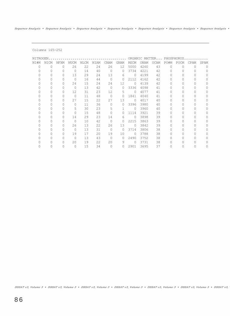
Sequence Analysis ¥ Sequence Analysis ¥ Sequence Analysis ¥ Sequence Analysis ¥ Sequence Analysis ¥ Sequence Analysis ¥ Sequence Analysis ¥
DSSAT v3, Volume 3 ¥ DSSAT v3, Volume 3 ¥ DSSAT v3, Volume 3 ¥ DSSAT v3, Volume 3 ¥ DSSAT v3, Volume 3 ¥ DSSAT v3, Volume 3 ¥ DSSAT v3, V
86
Columns 165-252
NITROGEN....................................... ORGANIC MATTER... PHOSPHORUS............NI#M NICM NFXM NUCM NLCM NIAM CNAM GNAM RECM ONAM OCAM PO#M POCM CPAM SPAM
0 0 0 26 22 24 26 12 5000 4260 43 0 0 0 00 0 0 0 14 40 0 0 3734 4221 42 0 0 0 00 0 0 13 29 24 13 6 0 4199 42 0 0 0 00 0 0 0 16 44 0 0 2112 4162 42 0 0 0 00 0 0 24 15 24 24 12 0 4139 42 0 0 0 00 0 0 0 13 42 0 0 3336 4098 41 0 0 0 00 0 0 12 31 23 12 5 0 4077 41 0 0 0 00 0 0 0 11 48 0 0 1841 4040 41 0 0 0 00 0 0 27 15 22 27 13 0 4017 40 0 0 0 00 0 0 0 11 36 0 0 3396 3980 40 0 0 0 00 0 0 5 30 23 5 1 0 3960 40 0 0 0 00 0 0 0 15 48 0 0 1114 3921 39 0 0 0 00 0 0 14 29 23 14 6 0 3898 39 0 0 0 00 0 0 0 10 42 0 0 2215 3863 39 0 0 0 00 0 0 26 13 22 26 13 0 3842 39 0 0 0 00 0 0 0 13 31 0 0 3714 3806 38 0 0 0 00 0 0 19 17 20 19 10 0 3788 38 0 0 0 00 0 0 0 13 43 0 0 2490 3752 38 0 0 0 00 0 0 20 19 22 20 9 0 3731 38 0 0 0 00 0 0 0 15 34 0 0 2901 3695 37 0 0 0 0

equence Analysis ¥ Sequence Analysis ¥ Sequence Analysis ¥ Sequence Analysis ¥ Sequence Analysis ¥ Sequence Analysis ¥ Sequence Analysis ¥ Sequence
¥ DSSAT v3, Volume 3 ¥ DSSAT v3, Volume 3 ¥ DSSAT v3, Volume 3 ¥ DSSAT v3, Volume 3 ¥ DSSAT v3, Volume 3 ¥ DSSAT v3, Volume 3 ¥ DSSAT v3, Volume
87
0 002 No entries found in file :The FILEX experimental listing file was found, but it contains no valid entries.
1 003 Cannot find file :The specified file cannot be found (non-fatal).
0 004 Error reading :An undefined read error occurred when attempting to read the file. The problemis usually caused by incorrect format of the file.
0 005 No valid treatments found in file :No valid treatments were found in the FILEX selected.
0 006 Error in *SIMULATION CONTROL factor levels :The FILEX specified by the user is defective in one of the following ways:FNAME was not set or not found, NREPS was not set or not found, or the simu-lation control factor level with the lowest number specified by the user did nothave a corresponding *SIMULATION CONTROL block in the file.
0 007 Error in *CULTIVAR factor levels in file :A cultivar factor level was specified in the selected FILEX that did not have a cor-responding cultivar description in the *CULTIVARS block of the file.
1 008 Model runs completed!
1 009 SUMMARY.OUT renamed to SUMMARY.SQS
1 010 SEQUENCE.LST updated, added file :Specified summary output file added to the listing file.
0 011 A required file was not found .. aborting :This usually refers to the absence of the file DSSATPRO.FLE, which could not befound.
0 012 Excessive path length error :You need to reduce the path length as specified in DSSATPRO.FLE for the cropmodel ÒccÓ (e.g. MZ). Path lengths as specified in the DSSATPRO.FLE must beless than 36 characters in total length, including drive letter, colon, and leadingand trailing slashes (\). If these paths are modified using the SETUP menu of theDSSAT3 shell, then there is no problem, as the screens will not allow you to enterpaths longer than this. If you modify DSSATPRO.FLE with a text editor, thenyou need to ensure that this total length is not exceeded.

Sequence Analysis ¥ Sequence Analysis ¥ Sequence Analysis ¥ Sequence Analysis ¥ Sequence Analysis ¥ Sequence Analysis ¥ Sequence Analysis ¥
DSSAT v3, Volume 3 ¥ DSSAT v3, Volume 3 ¥ DSSAT v3, Volume 3 ¥ DSSAT v3, Volume 3 ¥ DSSAT v3, Volume 3 ¥ DSSAT v3, Volume 3 ¥ DSSAT v3, V
88
0 013 No code error :The crop code specified (e.g. MZ) could not be found in the file DSSATPRO.FLE.This will occur if a cultivar is specified in FILEX that does not have a valid cropcode.
0 014 Read error in file :An undefined read error occurred when reading the specified file; check the for-mat of the file.
0 015 Rotation Option feature not yet implemented; file :The specified FILEX contained a value for the rotation option ÒOÓ other than 1;exit and fix the file.
0 016 SEQDRV: READ error, file :A read error occurred while the sequence driver was reading the specified file.
0 017 SEQDRV:A sequence driver error occurred; check the format of FILEX.
0 018 Last model run could not be completed as specifiedCheck the format and contents of FILEX; if this error occurs, then the simulationsummary output file may not be analyzable.
0 019 This run mode is not yet implemented
0 020 A problem was encountered executing another programThe driver was not able to execute another program; check the free RAM that youhave on your computer, and increase it if possible by unloading unnecessary resi-dent programs (e.g. a network).
0 021 A problem was encountered erasing a fileThe specified file could not be erased.
0 022 A problem was encountered copying a fileThe specified file could not be copied successfully.
1 055 Problem in finding the appropriate help screenThe required help screen, or the help screen file SEQDRV.HLP, could not befound.
1 100 Error!Undetermined error.

equence Analysis ¥ Sequence Analysis ¥ Sequence Analysis ¥ Sequence Analysis ¥ Sequence Analysis ¥ Sequence Analysis ¥ Sequence Analysis ¥ Sequence
¥ DSSAT v3, Volume 3 ¥ DSSAT v3, Volume 3 ¥ DSSAT v3, Volume 3 ¥ DSSAT v3, Volume 3 ¥ DSSAT v3, Volume 3 ¥ DSSAT v3, Volume 3 ¥ DSSAT v3, Volume
89
CHAPTER FOUR.ANALYZING SEQUENCE ANALYSIS EXPERIMENTS
Having produced a summary simulation output file from a sequence experiment,the next step is to analyze this (the experiment may or may not be replicated). Abrief overview of the analysis programÕs capabilities follows, together with somegeneral usage notes. It should be noted that the analysis program can handle amaximum of 1000 separate model runs.
Figure 2 shows the major menu options available. The program does the follow-ing.
Biophysical Analysis. Calculates means, standard deviations, maxima andminima by year and by rotation component for any of the 35 summary output filevariables (a list of these is shown in Table 7). These can be plotted as box plots,cumulative function plots, mean-variance diagrams, coefficient of variation plots,or variance plots. All graphs can be screen dumped to a printer or output to a filefor plotting.
Economic Analysis. Calculates means, standard deviations, maxima andminima by year and by rotation component of economic returns, and plots theseas box plots, cumulative function plots, or mean-variance diagrams. Prices andcosts can be changed within a session, and price-cost variability can be includedin the analysis. Simple probability analysis can be carried out, where the userspecifies a threshold level of economic returns per hectare; the probability of thespecified sequence failing to meet this threshold in each sequence year is then cal-culated and can be plotted.
Any number of summary output files can be analyzed sequentially during onesession with the program. The user can also control the way in which hardcopyoutputs are produced from the graphics program.
While these analyses are being performed, results are written to a results file.The file can be printed from within the program, if required. At the completionof the session, the user can access this file and use the data contained within inany way required. For example, it could be edited for importing into a graphics,spreadsheet or statistics program.
OV E RV I E W

Sequence Analysis ¥ Sequence Analysis ¥ Sequence Analysis ¥ Sequence Analysis ¥ Sequence Analysis ¥ Sequence Analysis ¥ Sequence Analysis ¥
DSSAT v3, Volume 3 ¥ DSSAT v3, Volume 3 ¥ DSSAT v3, Volume 3 ¥ DSSAT v3, Volume 3 ¥ DSSAT v3, Volume 3 ¥ DSSAT v3, Volume 3 ¥ DSSAT v3, V
90
AN EX A M P L E
The analysis program is called from the ANALYSES main menu item of the DSSATv3 Shell and then the ÒSequenceÐAnalyzeÓ submenus (Screen 3, on followingpage). After an introductory screen, the main menu screen (Screen 4, on followingpage) is presented.
First you must select a sequence output file to analyze (i.e., a summary output filefrom a previously-run simulation). On selecting this item, the program searchesSEQUENCE.LST, the listing file that contains the available model summary outputfiles in the current directory (Table 3). These are presented to the user (see Screen5). Note that the entries in SEQUENCE.LST do not have to match the entries inEXP.LST, either in number or in order; you may have run and analyzed the experi-ments in a different order, for example.
Use the mouse or cursor keys to select the file EBAF1101.SQS in Screen 5. The pro-gram then gives the user the opportunity to change the name of the analysis resultsfile. By default, this will be the same as the summary output file, except the last let-ter of the extension will be ÒRÓ (for ÒresultsÓ). Note that file names are preservedacross all three steps of the sequence analysis procedure: if the model FILEX is
FIGURE 2. MENU OPTIONS FOR THE SEQUENCE ANALYSIS PROGRAM.
PERFORMPROBABILITY ANALYSIS
PLOT GRAPHS
TABULATE
SUMMARY STATISTICS
CALCULATE ECON-OMIC RETURNS
INCLUDE OR EXCLUDE FALLOWS
ACCESS APRICE FILE
SELECT ANALYSIS METHOD
QUIT BIOPHYSICALANALYSIS
SELECT 1 OF 35OUTPUT VARIABLES
SELECT CROP CODES
ECONOMIC ANAYLSIS
SELECT MODELOUTPUT FILE
SELECT GRAPHICSHARDCOPY OPTIONS
CALCULATE & TABULATESUMMARY STATISTICS
PLOT GRAPHS PERFORM REGRESSIONS
PLOT REGRESSIONSAND RESIDUALS
EDIT A PRICE FILE

equence Analysis ¥ Sequence Analysis ¥ Sequence Analysis ¥ Sequence Analysis ¥ Sequence Analysis ¥ Sequence Analysis ¥ Sequence Analysis ¥ Sequence
¥ DSSAT v3, Volume 3 ¥ DSSAT v3, Volume 3 ¥ DSSAT v3, Volume 3 ¥ DSSAT v3, Volume 3 ¥ DSSAT v3, Volume 3 ¥ DSSAT v3, Volume 3 ¥ DSSAT v3, Volume
91
SCREEN 3.
SCREEN 4.
EBAF1101.SQX, then simulation results from the model(s) are saved inEBAF1101.SQS, and analysis results in EBAF1101.SQR. If you want to change theresults file name, enter a new name (8 characters maximum). Do not add the
S SeasonalQ Sequence
DECISION SUPPORT SYSTEM FOR AGROTECHNOLOGY TRANSFER
DATA MODEL ANALYSES TOOLS SETUP/QUIT
ESCmoves through menu choicesmoves to higher menu level Version: 3.0
↑ ↓ → ←
C Create
I Inputs
S Simulate
O Outputs
A Analyze
Analyze model outputs.
F1 (Help) 71440 Mem
Main Menu
Select a cropping season file for analysis
Analyse Biophysical variables
Analyse Economic variables
Modify hardopy options
About SUSTAIN2 ....
Exit
DSSAT Version 3.0 Crop Sequencing Analysis
Analyze model outputs.

Sequence Analysis ¥ Sequence Analysis ¥ Sequence Analysis ¥ Sequence Analysis ¥ Sequence Analysis ¥ Sequence Analysis ¥ Sequence Analysis ¥
DSSAT v3, Volume 3 ¥ DSSAT v3, Volume 3 ¥ DSSAT v3, Volume 3 ¥ DSSAT v3, Volume 3 ¥ DSSAT v3, Volume 3 ¥ DSSAT v3, Volume 3 ¥ DSSAT v3, V
92
extension; this is added automatically, and cannot be changed, and will always beÒccRÓ where ÒccÓ is the crop code (usually SQ for sequence analysis).
If the summary output file chosen contains more than 1 treatment, you will beasked to select which treatment to analyze. If there are more than 10 treatmentsin the file, then you may select only from amongst the first 10; the rest will beignored.
The next screen presented (Screen 6, on following page) summarizes the simula-tion runs found in the chosen summary output file. The experiment code, num-ber of runs and replicates, starting and ending year of the sequence, the numberof model runs per replicate, the number of runs per rotation (i.e., the number ofcrop components as specified in FILEX), and the crop codes used, are shown tothe user. If there are problems with the summary output file, for instance anunequal number of replicates because of model failure for some reason, theseproblems will usually be apparent at this stage. Such errors are usually trappedby the analysis program and result in a warning message to the user and termi-nation of the program.
Note that in the ÒCrop Codes UsedÓ portion of Screen 6, each crop code is fol-lowed by an integer. This is to allow analyses to be made on each separate cropcomponent specified in the original FILEX that controlled the sequence experi-
F1 (Help) 71440 Mem
Main Menu
FILE
UFGA7803 SQS SEQUENCE ANALYSIS, SIMPLE MULTI-TREAT FILE, 5:5 ....
UFGA7804 SQS BN-BN YR 1, SB YR 2 EXAMPLE, 10:5 ..................
EBAF1101 SQS MZ-FA, 30 YRS, 15 REPS, NO N .......................
Modify hardcopy options
About SUSTAIN2 ....
Exit
DSSAT Version 3.0 Crop Sequencing Analysis
EXT ENAME
SCREEN 5.
71440

equence Analysis ¥ Sequence Analysis ¥ Sequence Analysis ¥ Sequence Analysis ¥ Sequence Analysis ¥ Sequence Analysis ¥ Sequence Analysis ¥ Sequence
¥ DSSAT v3, Volume 3 ¥ DSSAT v3, Volume 3 ¥ DSSAT v3, Volume 3 ¥ DSSAT v3, Volume 3 ¥ DSSAT v3, Volume 3 ¥ DSSAT v3, Volume 3 ¥ DSSAT v3, Volume
93
ment. In some rotations, you may have 2 or more fallow components (onebetween maize and beans and another between beans and maize, for example).In both biological and economic terms, these fallows may be quite different, andneed to be treated separately.
On pressing any key to continue, the main menu of the analysis program appearsagain (Screen 4). The items in this menu are illustrated in turn.
Input File Analysis
Experiment Code : EBAF 11 01Number of runs : 900Number of reps : 15Starting year : 1911Ending year : 1941Runs per rep : 60Runs per rotation : 2Crop Codes Used : MZ1 FA1
DSSAT Version 3.0 Crop Sequencing Analysis
F1 (Help) Press any key to continue.. 71440 Mem
SCREEN 6.
AN A LY Z E B I O P H Y S I C A L VA R I A B L E S
On choosing the main menu option, ÒAnalyze Biophysical Variables,Ó in Screen 4,with the mouse or cursor keys, a list of the variables available for analysisappears (Screen 7, on following page). This is a listing of all the 35 output vari-ables written to the summary output file. You can scroll up and down this listusing the <> and <¯> arrow keys on the keyboard. Choose the variable, ÒHARYIELD kg/ha ,Ó in Screen 7 by placing the cursor bar over the variable in the listand pressing the <ENTER> key.
The next screen presented (Screen 8, on following page) asks you to choose a cropcode for analysis. Choose the MZ1 component (multiple crop codes are dis-cussed below). Thus, we have now selected to look at maize yields.
71440

Sequence Analysis ¥ Sequence Analysis ¥ Sequence Analysis ¥ Sequence Analysis ¥ Sequence Analysis ¥ Sequence Analysis ¥ Sequence Analysis ¥
DSSAT v3, Volume 3 ¥ DSSAT v3, Volume 3 ¥ DSSAT v3, Volume 3 ¥ DSSAT v3, Volume 3 ¥ DSSAT v3, Volume 3 ¥ DSSAT v3, Volume 3 ¥ DSSAT v3, V
94
Select a cropping season file for analysis
Analyse Biological variables
Analyse Economic variables
Modify hardopy options
About VARAN2....
Exit
F1 (Help) 71440 Mem
Main Menu
DSSAT Version 3.0 Crop Sequencing Analysis
Analysis
START SIM day
PLANTING day
ANTHESIS day
MATURITY day
HARVEST day
SOWING WT kg/ha
TOPS WT. kg/ha
MAT YIELD kg/ha
HAR YIELD kg/ha
BYPRODUCT kg/ha
WEIGHT mg/unit
NUMBER #/m2
NUMBER #/unit
IRRIG APPS #
IRRIG mm
PRECIP mm
ET TOTAL mm
RUNOFF mm ↑ ↓
SCREEN 7.
Select a cropping season file for analysis
Analyse Biological variables
Analyse Economic variables
Modify hardopy options
About VARAN2....
Exit
F1 (Help) 71440 Mem
Main Menu
DSSAT Version 3.0 Crop Sequencing Analysis
Analysis
START SIM day
PLANTING day
ANTHESIS day
MATURITY day
HARVEST day
SOWING WT kg/ha
TOPS WT. kg/ha
MAT YIELD kg/ha
HAR YIELD kg/ha
BYPRODUCT kg/ha
WEIGHT mg/unit
NUMBER #/m2
NUMBER #/unit
IRRIG APPS #
IRRIG mm
PRECIP mm
ET TOTAL mm
RUNOFF mm ↑ ↓
Crop codes
1 MZ1 [√]
2 FA1 [ ]
SCREEN 8.

equence Analysis ¥ Sequence Analysis ¥ Sequence Analysis ¥ Sequence Analysis ¥ Sequence Analysis ¥ Sequence Analysis ¥ Sequence Analysis ¥ Sequence
¥ DSSAT v3, Volume 3 ¥ DSSAT v3, Volume 3 ¥ DSSAT v3, Volume 3 ¥ DSSAT v3, Volume 3 ¥ DSSAT v3, Volume 3 ¥ DSSAT v3, Volume 3 ¥ DSSAT v3, Volume
95
The next screen (Screen 9, above ) shows the results of the calculations by theprogram. The screen is headed ÒTrends Over Time,Ó as the trends in maizeyields may well be what we are interested in. The output variable is shown(yield per hectare), together with the pertinent crop code (maize). For eachappearance of the chosen crop component, the program displays the mean, stan-dard deviation and minimum and maximum values of the selected variable. Inthe example, maize was grown each season, so an annual yield is displayed forthe years 1911 to 1940 (remember, the year numbers are purely for convenience inthis example). The experiment was replicated; if there were only one replicate,then the standard deviation would be zero, and the mean, the minimum and themaximum yield would be identical.
Press any key to continue, and repeat until the Graphics-Regression main menuscreen appears (Screen 10, on following page). If at any time you forget whichvariable you are looking at or which crop components are being analyzed, movethe cursor bar to the ÒAbout this plotÓ option to remind yourself. Five types ofgraphs can be plotted, described as follows.
Select a cropping season file for analysis
Analyse Biological variables
Analyse Economic variables
Modify hardopy options
About VARAN2....
Exit
F1 (Help) 71440 Mem
Main Menu
DSSAT Version 3.0 Crop Sequencing Analysis
Analysis1
2
3
4
5
6
7
8
9
10
11
12
13
14
15
16
17
18
START SIM day [ ]
PLANTING day [ ]
ANTHESIS day [ ]
MATURITY day [ ]
HARVET day [ ]
SOWING WT kg/ha [ ]
TOPS WT. kg/ha [ ]
MAT YIELD kg/ha [ ]
HAR YIELD kg/ha [ ]
BYPRODUCT kg/ha [ ]
WEIGHT mg/unit [ ]
NUMBER #/m2 [ ]
NUMBER #/unit [ ]
IRRIG APPS # [ ]
IRRIG mm [ ]
PRECIP mm [ ]
ET TOTAL mm [ ]
RUNOFF mm [ ]
↑ ↓
Trends Over Time
Variable : HAR YIELD kg/haCrop Code(s) : MZ1
Sequence Year Mean St.Dev. Min Max
1911.0
1912.0
1913.0
1914.0
1915.0
1916.0
1917.0
1918.0
1919.0
1920.0
2223.9
1087.5
1401.0
1242.3
1206.8
1323.1
971.6
913.9
1107.2
1291.9
406.0
394.2
559.2
674.8
587.8
614.0
621.6
500.1
632.0
539.4
1708.0
517.0
480.0
183.0
132.0
164.0
80.0
114.0
400.0
129.0
3041.0
1992.0
1987.0
2530.0
1970.0
2102.0
1955.0
2111.0
2467.0
2363.0
Press any key to see more ..
SCREEN 9.
71440

Sequence Analysis ¥ Sequence Analysis ¥ Sequence Analysis ¥ Sequence Analysis ¥ Sequence Analysis ¥ Sequence Analysis ¥ Sequence Analysis ¥
DSSAT v3, Volume 3 ¥ DSSAT v3, Volume 3 ¥ DSSAT v3, Volume 3 ¥ DSSAT v3, Volume 3 ¥ DSSAT v3, Volume 3 ¥ DSSAT v3, Volume 3 ¥ DSSAT v3, V
96
OPTION 1. BOX PLOT
If this option is selected in Screen 10, a box plot appears (Screen 11, on followingpage). (by default, all years are selected for plotting box plots). The box plot is away of assessing visually the variability over time of the output variable underconsideration. For the distribution of the model output variable selected, the 0th(the lowest single short line), 25th (the lower of the short lines connected by thevertical bar), 50th (the star), 75th (the upper of the short lines connected by thevertical bar), and 100th (the upper single short line) percentiles are plotted. The50th percentile is the median of each output variable distribution, not the mean;but for symmetrical distributions, the median will often not differ greatly fromthe mean value.
This graph may be plotted on your printer by pressing the <P> key while thegraph is on the screen. If the graph does not plot, you may need to change hard-copy settings (refer to the section, ÒGraphics Hardcopy SetupÓ). Depending onthe printer and the resolution used, there may be a delay of a few seconds whilethis is done; wait for the graph to show on the screen again before continuing.
Select a cropping season file for analysis
Analyse Biological variables
Analyse Economic variables
Modify hardopy options
About VARAN2....
Exit
START SIM day
PLANTING day
ANTHESIS day
MATURITY day
HARVET day
SOWING WT kg/ha
TOPS WT. kg/ha
MAT YIELD kg/ha
HAR YIELD kg/ha
BYPRODUCT kg/ha
WEIGHT mg/unit
NUMBER #/m2
NUMBER #/unit
IRRIG APPS #
IRRIG mm
PRECIP mm
ET TOTAL mm
RUNOFF mm
F1 (Help) 71440 Mem
Main Menu
DSSAT Version 3.0 Crop Sequencing Analysis
Analysis
↑ ↓
Trends Over Time
Box plot
Cumulative function plot
Mean-Variance plot
Variance plot
Coefficient of variation plot
Regression menu
About this plot
Quit ...
SCREEN 10.
GR A P H I C S -RE G R E S S I O N MA I N ME N U
71440

BOX PLOT OF HAR YIELD kg/ha MZ1
HAR YIELD kg/ha
YEAR
3.200k
2.800k
2.400k
2.00k
1.600k
1.200k
0.800k
0.400k
1.918k 1.926k 1.934k
❊
❊
❊
❊
❊❊
❊❊
❊
❊
❊
❊
❊ ❊
❊
❊
❊
❊
❊
❊
❊
❊
❊
❊❊ ❊
❊
❊
❊
❊
HWAH
1.910k 1.942k
equence Analysis ¥ Sequence Analysis ¥ Sequence Analysis ¥ Sequence Analysis ¥ Sequence Analysis ¥ Sequence Analysis ¥ Sequence Analysis ¥ Sequence
¥ DSSAT v3, Volume 3 ¥ DSSAT v3, Volume 3 ¥ DSSAT v3, Volume 3 ¥ DSSAT v3, Volume 3 ¥ DSSAT v3, Volume 3 ¥ DSSAT v3, Volume 3 ¥ DSSAT v3, Volume
97
NOTE: To return to the analysis program from any graph, press any key.
OPTION 2. CUMULATIVE FUNCTION PLOT
When this option is selected in Screen 10, output variables by year or season mayalso be plotted as cumulative function plots. (Cumulative function plots aresometimes called cumulative probability function (CPF) plots or cumulative dis-tribution function plots Ð these are the same.) Here, the distribution for the cho-
SCREEN 11.
1918 1926 1934 1.942k
HWAH

Sequence Analysis ¥ Sequence Analysis ¥ Sequence Analysis ¥ Sequence Analysis ¥ Sequence Analysis ¥ Sequence Analysis ¥ Sequence Analysis ¥
DSSAT v3, Volume 3 ¥ DSSAT v3, Volume 3 ¥ DSSAT v3, Volume 3 ¥ DSSAT v3, Volume 3 ¥ DSSAT v3, Volume 3 ¥ DSSAT v3, Volume 3 ¥ DSSAT v3, V
98
sen output variable for each season or year is ordered from smallest to largest,and plotted against equal increments of cumulative probability.
After selecting this option, the year selection screen appears (Screen 12, below),allowing the user to select which yearsÕ values are to be plotted in this way. Amaximum of six CPF plots may be graphed at any time, to reduce the confusionof the plot. You can select or deselect years all at once with the <+> or the <->key, or individually with the space bar. If more than six years are selected, theprogram will plot the first six years selected; the rest will be ignored.
For the example, select the years 1911, 1913, 1915, 1917, 1919, and 1921 (as shownin Screen 12), and press the <ENTER> key. The resulting plot is shown in Screen13 (on following page). To print, press the <P> key, or press the <ENTER> key toreturn the Graphics-Regression main menu (Screen 10).
SCREEN 12.
Select a cropping season file for analysis
Analyse Biological variables
Analyse Economic variables
Modify hardopy options
About VARAN2....
Exit
START SIM day
PLANTING day
ANTHESIS day
MATURITY day
HARVET day
SOWING WT kg/ha
TOPS WT. kg/ha
MAT YIELD kg/ha
HAR YIELD kg/ha
BYPRODUCT kg/ha
WEIGHT mg/unit
NUMBER #/m2
NUMBER #/unit
IRRIG APPS #
IRRIG mm
PRECIP mm
ET TOTAL mm
RUNOFF mm
F1 (Help) 71440 Mem
Main Menu
DSSAT Version 3.0 Crop Sequencing Analysis
Analysis
↑ ↓
Trends Over Time
Box plot
Cumulative function plot
Mean-Variance plot
Variance plot
Coefficient of variation plot
Regression menu
About this plot
Quit ...
↑ ↓
1
2
3
4
5
6
7
8
9
10
11
12
13
14
15
16
1911.0 [√]1912.0 [ ]
1913.0 [√]1914.0 [ ]
1915.0 [√]1916.0 [ ]
1917.0 [√]1918.0 [ ]
1919.0 [√]1920.0 [ ]
1921.0 [√]1922.0 [ ]
1923.0 [ ]
1924.0 [ ]
1925.0 [ ]
1926.0 [ ]
# YEAR
71440

equence Analysis ¥ Sequence Analysis ¥ Sequence Analysis ¥ Sequence Analysis ¥ Sequence Analysis ¥ Sequence Analysis ¥ Sequence Analysis ¥ Sequence
¥ DSSAT v3, Volume 3 ¥ DSSAT v3, Volume 3 ¥ DSSAT v3, Volume 3 ¥ DSSAT v3, Volume 3 ¥ DSSAT v3, Volume 3 ¥ DSSAT v3, Volume 3 ¥ DSSAT v3, Volume
99
OPTION 3. MEAN-VARIANCE PLOT
When this option in Screen 10 is selected, output variables may be plotted inmean-variance space. The calculated mean is plotted against the variance for theoutput variable of interest, and the sequence year numbers themselves are drawnon the graph. All the seasons available may be plotted in this way, or you maychoose a subset of seasons to avoid confusion on the graph. Such graphs areanother way of giving an indication of the variability associated with each seasonin the sequence, and are useful for visualizing the tradeoffs that must sometimes
CPF PLOT OF HAR YIELD kg/ha MZ1
1.000
0.800
0.600
0.400
0.200
CUMULATIVE PROBABILITY
0.400k 0.800k 1.200k 1.600k 2.000k 2.400k 2.800k
(1) 1911.0(1) 1915.0(1) 1919.0
(1) 1913.0(1) 1917.0(1) 1921.0
1911.0
1915.0
1919.0
1913.0
1917.0
1921.0
0 3.200k
SCREEN 13.

Sequence Analysis ¥ Sequence Analysis ¥ Sequence Analysis ¥ Sequence Analysis ¥ Sequence Analysis ¥ Sequence Analysis ¥ Sequence Analysis ¥
DSSAT v3, Volume 3 ¥ DSSAT v3, Volume 3 ¥ DSSAT v3, Volume 3 ¥ DSSAT v3, Volume 3 ¥ DSSAT v3, Volume 3 ¥ DSSAT v3, Volume 3 ¥ DSSAT v3, V
100
1
2
3
10
17
5
6
4
15
1422 8
1619
24
9
71213
27
212620
3011
29
18
23
2528
100.0k 200.0k 300.0k 400.0k
2.500k
2.000k
1.500k
1.000k
0.500k
MEAN
E-V PLOT OF HAR YIELD kg/ha
VARIANCE
HWAH
0 500.0k
SCREEN 14.
HWAH
VARIANCE
MEAN
be made between striving for a higher mean value while increasing the variabili-ty (as described by the variance) for the output of interest.
Choose the mean-variance plot option to produce the plot (Screen 14, below).The y-axis for such a plot is always scaled automatically, and care will sometimesbe needed in interpretation, as the difference between the means (i.e., the differ-ence from the top to the bottom of the scale) may not be very much, and willsometimes be much less than appears from a cursory glance at the graph. Toprint the plot, press the <P> key, or press any key to return to the Graphics-Regression main menu (Screen 10).

equence Analysis ¥ Sequence Analysis ¥ Sequence Analysis ¥ Sequence Analysis ¥ Sequence Analysis ¥ Sequence Analysis ¥ Sequence Analysis ¥ Sequence
¥ DSSAT v3, Volume 3 ¥ DSSAT v3, Volume 3 ¥ DSSAT v3, Volume 3 ¥ DSSAT v3, Volume 3 ¥ DSSAT v3, Volume 3 ¥ DSSAT v3, Volume 3 ¥ DSSAT v3, Volume
101
OPTION 4. VARIANCE PLOT
If this option is selected in Screen 10, a time series is produced (Screen 15, below)of the variance of the output variable chosen over the length of the sequence. Thevariance will often be of use in determining whether variability in the system isincreasing or decreasing over time. If it is increasing, then this may be an indica-tion of long-term problems in the system leading to unsustainable performance, forexample.
There will be some output variables where no change in variance is expected over
VARIANCE PLOT OF HAR YIELD kg/ha MZ1
500.0k
400.0k
300.0k
200.0k
100.0k
VARIANCE
1917 1923 1929 1935
YEAR
HWAH
1911 1941
SCREEN 15.
HWAH
1917 1923 1929 1935
VARIANCE

Sequence Analysis ¥ Sequence Analysis ¥ Sequence Analysis ¥ Sequence Analysis ¥ Sequence Analysis ¥ Sequence Analysis ¥ Sequence Analysis ¥
DSSAT v3, Volume 3 ¥ DSSAT v3, Volume 3 ¥ DSSAT v3, Volume 3 ¥ DSSAT v3, Volume 3 ¥ DSSAT v3, Volume 3 ¥ DSSAT v3, Volume 3 ¥ DSSAT v3, V
102
time, such as in seasonal rainfall. If there is a clear trend in seasonal rainfall andyou have used one of the weather generators, for example, this is clear indicationof a serious problem (BUT refer to the Appendix). Return to the Graphic-Regression main menu (Screen 10) by pressing any key.
OPTION 5. COEFFICIENT OF VARIATION PLOT
The fifth graphics option in Screen 10 allows you to plot the coefficient of varia-tion of the selected output variable, calculated as (s/x) * 100, where s is the stan-dard deviation and x the mean, against time. This type of plot can give a useful
120.0
90.0
60.0
30.0
CV, %
COEFFICIENT OF VARIATION PLOT OF HAR YIELD kg/ha MZ1
1917 1923 1929 1935
YEAR
(1) HWAH
1911 1941
SCREEN 16.
1917 1923 1929 1935
HWAH

equence Analysis ¥ Sequence Analysis ¥ Sequence Analysis ¥ Sequence Analysis ¥ Sequence Analysis ¥ Sequence Analysis ¥ Sequence Analysis ¥ Sequence
¥ DSSAT v3, Volume 3 ¥ DSSAT v3, Volume 3 ¥ DSSAT v3, Volume 3 ¥ DSSAT v3, Volume 3 ¥ DSSAT v3, Volume 3 ¥ DSSAT v3, Volume 3 ¥ DSSAT v3, Volume
103
indication of changes in relative variability through time. Screen 16 (on previouspage) shows an example for maize yield. Note that although mean yielddecreased through time, relative variability, as measured by the coefficient ofvariation, increased markedly.
Return to the Graphics-Regression main menu (Screen 10) by pressing any key.
OPTION 6. REGRESSION MENU
Choose the ÒRegression MenuÓ option in Screen 10. The screen that appears(Screen 17, below) gives you the option of calculating a linear or exponentialregression on the means of the seasonal output variable. The regression line withthe original means can be plotted, as can the residuals from the regression.
If you have not yet read the nAppendix, then please do so now. It cannot beover-emphasized that the potential to produce spurious results is high at thisstage in the analysis program. To reiterate a major conclusion of Appendix A,the chances of obtaining a meaningful regression of means with less than 10replicates of the sequence are slim. You are urged to exercise caution in interpret-ing such analyses, and this is not something the program can do Ñ your owncommon sense must prevail.
Select a cropping season file for analysis
Analyse Biological variables
Analyse Economic variables
Modify hardopy options
About VARAN2....
Exit
START SIM day
PLANTING day
ANTHESIS day
MATURITY day
HARVET day
SOWING WT kg/ha
TOPS WT. kg/ha
MAT YIELD kg/ha
HAR YIELD kg/ha
BYPRODUCT kg/ha
WEIGHT mg/unit
NUMBER #/m2
NUMBER #/unit
IRRIG APPS #
IRRIG mm
PRECIP mm
ET TOTAL mm
RUNOFF mm
F1 (Help) 71440 Mem
Main Menu
DSSAT Version 3.0 Crop Sequencing Analysis
Analysis
↑ ↓
Trends Over Time
Box plot
Cumulative function plot
Mean-Variance plot
Variance plot
Coefficient of variation plot
Regression menu
About this plot
Quit ...
Do a linear regression
Do an exponential regression
Plot the regression line
Plot the regression residuals
Quit
Regression of Means
SCREEN 17.

Sequence Analysis ¥ Sequence Analysis ¥ Sequence Analysis ¥ Sequence Analysis ¥ Sequence Analysis ¥ Sequence Analysis ¥ Sequence Analysis ¥
DSSAT v3, Volume 3 ¥ DSSAT v3, Volume 3 ¥ DSSAT v3, Volume 3 ¥ DSSAT v3, Volume 3 ¥ DSSAT v3, Volume 3 ¥ DSSAT v3, Volume 3 ¥ DSSAT v3, V
104
REGRESSION MENU
From the regression menu, you must first choose to do a regression before plot-ting it or the residuals.
Linear Regression. To illustrate, choose the option, ÒDo a linear regres-sion,Óin Screen 17. The resulting screen (Screen 18, below) gives the output, interms of the calculated constant or intercept, the slope or gradient, the quantityr2, the standard error of the gradient, and a t-test that tests the hypothesis thatthe gradient is significantly different from 0. The meaning of these outputs is asfollows (from Snedecor and Cochran, 1980).
The program performs a simple least-squares regression and fits the followingline to the data points:
y = mx + cwhere y is the output variable under consideration (here, yield), m is the slope orgradient, x is the year number, and c is a constant (the y-axis intercept, or thevalue of y when x equals zero). The quantity r2 can be interpreted as the estimat-ed proportion of the variance of y that can be attributed to its linear regression onx. The hypothesis that the gradient is significantly different from zero (i.e., a
Select a cropping season file for analysis
Analyse Biological variables
Analyse Economic variables
Modify hardopy options
About VARAN2....
Exit
START SIM day
PLANTING day
ANTHESIS day
MATURITY day
HARVET day
SOWING WT kg/ha
TOPS WT. kg/ha
MAT YIELD kg/ha
HAR YIELD kg/ha
BYPRODUCT kg/ha
WEIGHT mg/unit
NUMBER #/m2
NUMBER #/unit
IRRIG APPS #
IRRIG mm
PRECIP mm
ET TOTAL mm
RUNOFF mm
F1 (Help) 71440 Mem
Main Menu
DSSAT Version 3.0 Crop Sequencing Analysis
Analysis
↑ ↓
Variable : HAR YIELD kg/ha
Crop Code(s) : MZ1
Type : Linear
Regression of Means
Constant =
Gradient =
R-squared =
Standard error of gradient = 5.212
T-test of gradient: significant at p = .000
66358.4100
-34.0009
.6039
SCREEN 18.
71440
equence Analysis ¥ Sequence Analysis ¥ Sequence Analysis ¥ Sequence Analysis ¥ Sequence Analysis ¥ Sequence Analysis ¥ Sequence Analysis ¥ Sequence
¥ DSSAT v3, Volume 3 ¥ DSSAT v3, Volume 3 ¥ DSSAT v3, Volume 3 ¥ DSSAT v3, Volume 3 ¥ DSSAT v3, Volume 3 ¥ DSSAT v3, Volume 3 ¥ DSSAT v3, Volume
105
trend exists) can be tested byt = m/sm
where t is distributed as StudentÕs t with n-2 degrees of freedom (sm is the standarderror of the gradient and n is the number of data points).
The model fitted,y = a + §x + e
where e is a random variable drawn from N(0,sx.y2), makes a number of assump-tions, including the following:
1. For each specific X there is a normal distribution of Y from which sample valuesof Y are drawn at random;
2. The normal distributions of Y for specific X are independent;3. The normal distributions of Y for specific X all have the same variance sx.y2.
All these assumptions are often violated when looking at trends in sequences: thedistribution of yields for any sequence year will often not be normal; the sequencedistributions are not independent, since yields in one year will be dependent tosome extent on yields in previous years; and the variances of output distributionsoften change markedly over the length of the sequence.
For these reasons, great care is needed in interpreting the regressions. A quick ideaof the likely significance of the regression can be gained from inspection of thevalue of r2; for the 10 or 20 data points that will often be used in the program, anyvalue less than 0.5 or so will indicate that the regression is not statistically signifi-cant.
In the example in Screen 18, the regression suggests that the slope or gradient isnegative (i.e., on average, there is a trend for maize yields to decrease by 34 kg/haeach season). The standard error of the gradient is not large, compared with itsvalue. The slope is significantly different from zero, according to the t-test. Theregression explains a fair proportion of the variability in mean yield, since the valueof r2 is moderate (0.6).
Exponential Regression. The exponential regression option operates in thesame way, by fitting the linear transformation
ln(y) = ln(c) + mxof the exponential function
y = c * exp(mx),notation as above.

Sequence Analysis ¥ Sequence Analysis ¥ Sequence Analysis ¥ Sequence Analysis ¥ Sequence Analysis ¥ Sequence Analysis ¥ Sequence Analysis ¥
DSSAT v3, Volume 3 ¥ DSSAT v3, Volume 3 ¥ DSSAT v3, Volume 3 ¥ DSSAT v3, Volume 3 ¥ DSSAT v3, Volume 3 ¥ DSSAT v3, Volume 3 ¥ DSSAT v3, V
106
Plot the Regression Line. Having fitted a regression, the regressionline can be plotted; choose this option from the Regression menu (Screen 17) toproduce the plot (Screen 19, below). The fitted line is shown together with theseasonal means as small boxes. Note that the yield for 1911 is much higher thanits regressed value. This is largely due to the 5 t/ha of crop residue added at thestart of each sequence replicate (see Table 2).
Press any key to return to the Regression menu.
2.500k
2.000k
1.500k
1.000k
0.500k
HAR YIELD kg/ha
REGRESSION PLOT OF HAR YIELD kg/ha MZ1
YEAR
(1) Yield at harvest (kg dm/ha)
1918 1926 19341910 1942
SCREEN 19.
Yield at harvest (kg dm/ha)
1918 1910 1926 1934

Plot the Regression Residuals. Now choose to plot the residuals (Screen 20,on following page). These are the deviations of the points Y from the fitted line,
dy.x = Y - Y = y - mxwhere Y is the regressed value of output and Y is the simulated value from the cropmodel. No trends or patterns should be discernible in the residuals; such patterns areevidence of serious violations of the assumption of statistical independence in particu-lar, and the resulting regression should be discarded or treated with caution.
To sum up, despite the patina of ÒobjectivityÓ that may be given to your simulatedresults using regression to find trends, you should exercise great care in interpretingthe outputs from the regression option. As noted above, there is no substitute for com-mon sense.
equence Analysis ¥ Sequence Analysis ¥ Sequence Analysis ¥ Sequence Analysis ¥ Sequence Analysis ¥ Sequence Analysis ¥ Sequence Analysis ¥ Sequence
¥ DSSAT v3, Volume 3 ¥ DSSAT v3, Volume 3 ¥ DSSAT v3, Volume 3 ¥ DSSAT v3, Volume 3 ¥ DSSAT v3, Volume 3 ¥ DSSAT v3, Volume 3 ¥ DSSAT v3, Volume
107
AN A LY Z I N G MO R E TH A N ON E CR O P AT A T I M E
The analysis program has the option for analyzing more than one crop at a time. Toillustrate, return to the Analyses main menu (Screen 4), again select the option,ÒAnalyze Biophysical Variables,Ó and then choose the variable precipitation (PRECIPmm) from Screen 7, and pick both crop codes as shown in Screen 21 (on second fol-lowing page.)
The resulting screen warns you that you have picked multiple crop codes. In the sub-sequent screen (Screen 22, on second following page), you have to make a choice as tohow the program will analyze these multiple crops. There are three options,described as follows.
Option 1 - Additive. The values of the output variable for all selected crops willbe simply added together to provide a grand total by year of the output of interest;
Option2 - Average. The values of the output variable for all selected crops willbe averaged to provide a single ÒmeanÓ value of the output of interest for the relevantcalendar year;
Option 3 - Time Series. Each value of the output variable for all selected cropcodes will be treated independently to provide a time series of the output of interest.
Which option you choose will depend on the output variable and what you are tryingto achieve. It is important to understand the differences in these three options. Forexample, it may make sense to add total fertilizer applied across different crops; itmay not make much sense to add bean yields and maize yields if grown in the samegrowing season in the same calendar year.

Sequence Analysis ¥ Sequence Analysis ¥ Sequence Analysis ¥ Sequence Analysis ¥ Sequence Analysis ¥ Sequence Analysis ¥ Sequence Analysis ¥
DSSAT v3, Volume 3 ¥ DSSAT v3, Volume 3 ¥ DSSAT v3, Volume 3 ¥ DSSAT v3, Volume 3 ¥ DSSAT v3, Volume 3 ¥ DSSAT v3, Volume 3 ¥ DSSAT v3, V
108
193419261918
633.1
243.5
-146.1
-535.7
HAR YIELD kg/ha
(1) Yield at harvest (kg dm/ha)
YEAR
RESIDUALS, REGRESSION OF HAR YIELD kg/ha MZ1
1910 1942
SCREEN 20.
Yield at harvest (kg dm/ha)
1918 1926 19341910
Choose the ÒTime seriesÓ option in Screen 22 for looking at precipitation for themaize-fallow experiment. The resulting screen (Screen 23, on second followingpage) lists the mean, standard deviation, minimum and maximum rainfall bysequence year. Note that the sequence years have non-zero decimal points. Thetime series is produced by treating maize and fallow separately; for the firstreplicate, maize was harvested on day 59 in 1912 (see Table 4, data record 1,under HDAT), with a cumulative rainfall mean of 1213 mm (Table 4, data record1, under PRCM). For all 15 replicates, the mean harvest date was day 55.8 (youcan check this by analyzing the maize harvest date). Thus the sequence year
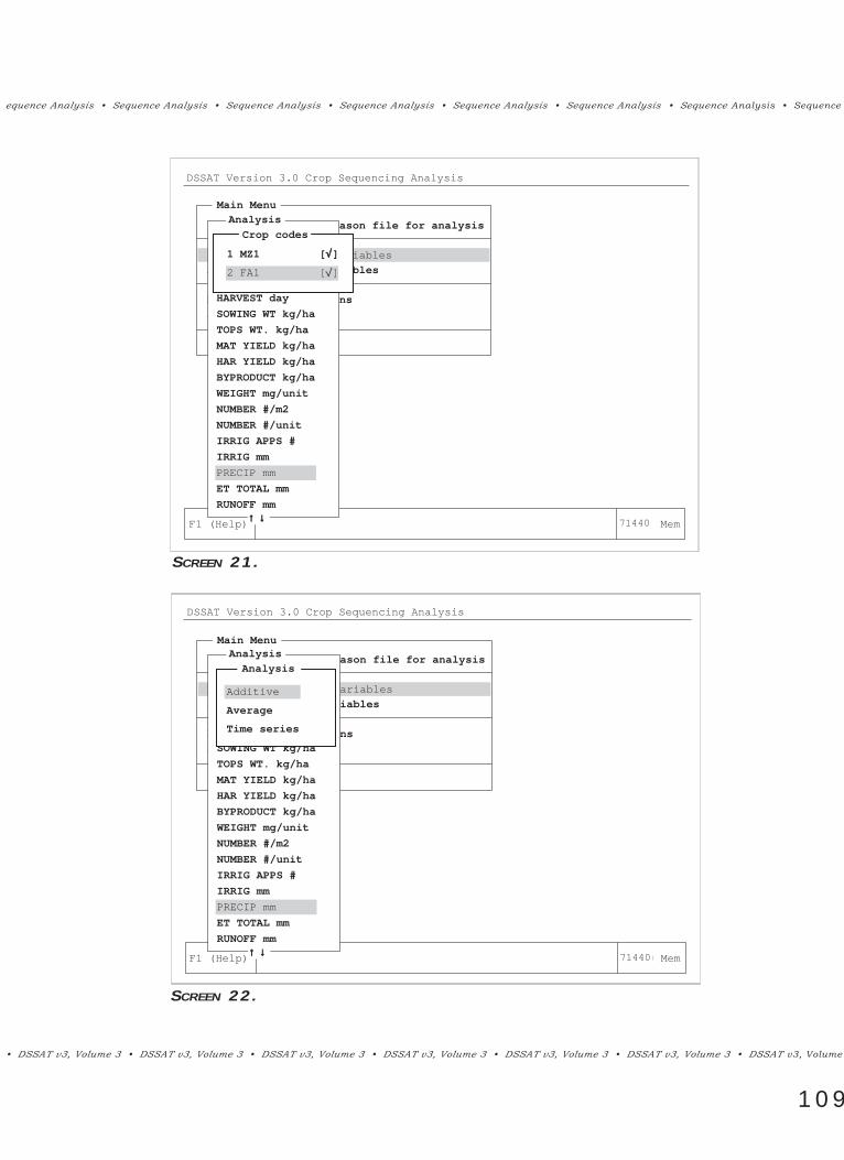
equence Analysis ¥ Sequence Analysis ¥ Sequence Analysis ¥ Sequence Analysis ¥ Sequence Analysis ¥ Sequence Analysis ¥ Sequence Analysis ¥ Sequence
¥ DSSAT v3, Volume 3 ¥ DSSAT v3, Volume 3 ¥ DSSAT v3, Volume 3 ¥ DSSAT v3, Volume 3 ¥ DSSAT v3, Volume 3 ¥ DSSAT v3, Volume 3 ¥ DSSAT v3, Volume
109
Select a cropping season file for analysis
Analyse Biological variables
Analyse Economic variables
Modify hardopy options
About VARAN2....
Exit
F1 (Help) 71440 Mem
Main Menu
DSSAT Version 3.0 Crop Sequencing Analysis
Analysis
START SIM day
PLANTING day
ANTHESIS day
MATURITY day
HARVEST day
SOWING WT kg/ha
TOPS WT. kg/ha
MAT YIELD kg/ha
HAR YIELD kg/ha
BYPRODUCT kg/ha
WEIGHT mg/unit
NUMBER #/m2
NUMBER #/unit
IRRIG APPS #
IRRIG mm
PRECIP mm
ET TOTAL mm
RUNOFF mm ↑ ↓
Crop codes
1 MZ1 [√]
2 FA1 [ ]
SCREEN 21.
Select a cropping season file for analysis
Analyse Biological variables
Analyse Economic variables
Modify hardopy options
About VARAN2....
Exit
F1 (Help) 71440 Mem
Main Menu
DSSAT Version 3.0 Crop Sequencing Analysis
Analysis
START SIM day
PLANTING day
ANTHESIS day
MATURITY day
HARVEST day
SOWING WT kg/ha
TOPS WT. kg/ha
MAT YIELD kg/ha
HAR YIELD kg/ha
BYPRODUCT kg/ha
WEIGHT mg/unit
NUMBER #/m2
NUMBER #/unit
IRRIG APPS #
IRRIG mm
PRECIP mm
ET TOTAL mm
RUNOFF mm ↑ ↓
Analysis
Additive
Average
Time series
SCREEN 22.
71440
71440
√

Sequence Analysis ¥ Sequence Analysis ¥ Sequence Analysis ¥ Sequence Analysis ¥ Sequence Analysis ¥ Sequence Analysis ¥ Sequence Analysis ¥
DSSAT v3, Volume 3 ¥ DSSAT v3, Volume 3 ¥ DSSAT v3, Volume 3 ¥ DSSAT v3, Volume 3 ¥ DSSAT v3, Volume 3 ¥ DSSAT v3, Volume 3 ¥ DSSAT v3, V
110
number is calculated as 1912+(55.8/365), or 1912.2 to one decimal place (Screen 23).
The first fallow period of the first replicate stopped on day 304 in 1912, as it did foreach year subsequently (Table 4): remember that planting of maize took place onday 305 each year. The mean sequence year number for the fallow rainfall total isthus calculated as 1912+(304/365), or 1912.8 to one decimal place. These are theyear numbers that are used in all subsequent plots. Thus a box plot of precipita-tion shows a time series of these cumulative rainfall occurrences (see Screen 24, onfollowing page).
You may notice that the rainfall amount for the maize crop in 1911 - 1912 appearshigher than in other years. This is explained by the fact that in 1911, simulationwith the maize model started on day 244 (Tables 2 and 4); in all other years, themaize model was run from day 305. Thus in 1911, the rainfall total covers a longerperiod than in any of the other years. This again illustrates the care that is neededin the interpretation of analysis results and the importance of understanding thenature of your crop sequence.
Now return to the Crop Code menu (Screen 21), choose MZ1 and FA1 as before,
Select a cropping season file for analysis
Analyse Biological variables
Analyse Economic variables
Modify hardopy options
About VARAN2....
Exit
F1 (Help) 71440 Mem
Main Menu
DSSAT Version 3.0 Crop Sequencing Analysis
Analysis1
2
3
4
5
6
7
8
9
10
11
12
13
14
15
16
17
18
START SIM day [ ]
PLANTING day [ ]
ANTHESIS day [ ]
MATURITY day [ ]
HARVET day [ ]
SOWING WT kg/ha [ ]
TOPS WT. kg/ha [ ]
MAT YIELD kg/ha [ ]
HAR YIELD kg/ha [ ]
BYPRODUCT kg/ha [ ]
WEIGHT mg/unit [ ]
NUMBER #/m2 [ ]
NUMBER #/unit [ ]
IRRIG APPS # [ ]
IRRIG mm [ ]
PRECIP mm [ ]
ET TOTAL mm [ ]
RUNOFF mm [ ]
↑ ↓Press any key to see more ..
Trends Over Time
Variable : PRECIP mmCrop Code(s) : MZ1 FA1
Sequence Year Mean St.Dev. Min Max
1912.2
1912.8
1913.2
1913.8
1914.1
1914.8
1915.2
1915.8
1916.2
1916.8
1050.9
638.1
893.1
636.3
846.6
631.2
872.5
614.7
880.7
557.8
137.3
100.1
113.5
134.8
99.2
124.8
157.2
145.8
141.4
163.2
763.0
519.0
711.0
438.0
632.0
380.0
589.0
336.0
712.0
392.0
1222.0
898.0
1174.0
914.0
1007.0
850.0
1131.0
892.0
1182.0
981.0
SCREEN 23.
71440

equence Analysis ¥ Sequence Analysis ¥ Sequence Analysis ¥ Sequence Analysis ¥ Sequence Analysis ¥ Sequence Analysis ¥ Sequence Analysis ¥ Sequence
¥ DSSAT v3, Volume 3 ¥ DSSAT v3, Volume 3 ¥ DSSAT v3, Volume 3 ¥ DSSAT v3, Volume 3 ¥ DSSAT v3, Volume 3 ¥ DSSAT v3, Volume 3 ¥ DSSAT v3, Volume
111
but this time choose Analysis Option 1 (Additive) in Screen 22. Observe the differ-ences in the tabular output and the plot; ÒmaizeÓ and ÒfallowÓ precipitations areadded together by the calendar year in which they occurred (according to harvestdates in the summary output file).
Now do the same thing, but choose Analysis Option 2 (Average) in Screen 22; theaverage values will be produced by calendar year. Note that this analysis has littlemeaning here, but it is useful for understanding the differences in the analysisoptions.
❊
❊
❊
❊
❊❊
❊
❊
❊
❊
❊
❊
❊
❊
❊
❊
❊
❊❊
❊
❊
❊
❊
❊
❊
❊❊
❊
❊
❊
❊
❊
❊
❊
❊
❊
❊
❊❊
❊
❊
❊
❊
❊❊
❊
❊
❊
❊
❊❊
❊
❊❊
❊
❊❊❊
❊
❊
1.400k
1.200k
1.000k
0.800k
0.600k
0.400k
Season precipitation (mm)
1919 1927 1935
YEAR
BOX PLOT OF PRECIP mm MZ1 FA1
PRECIP mm
1911 1943
SCREEN 24.
1919 1927 1935 1911
Season precipitation (mm)
Sequence Analysis ¥ Sequence Analysis ¥ Sequence Analysis ¥ Sequence Analysis ¥ Sequence Analysis ¥ Sequence Analysis ¥ Sequence Analysis ¥
DSSAT v3, Volume 3 ¥ DSSAT v3, Volume 3 ¥ DSSAT v3, Volume 3 ¥ DSSAT v3, Volume 3 ¥ DSSAT v3, Volume 3 ¥ DSSAT v3, Volume 3 ¥ DSSAT v3, V
112
The analysis program thus has the flexibility to analyze different combinations ofrotation components. Again, you should be careful in interpreting the results, asthey may not always be meaningful or useful.
AN A LY Z E EC O N O M I C VA R I A B L E S
Option 2, ÒAnalyze Economic Variables,Ó in the Sequence Analysis main menu(Screen 4) allows the analysis of the sequence in economic terms. On choosingthis option, the Economic Evaluation main menu appears (Screen 25, on follow-ing page). There are four major options, described below.
EC O N O M I C EVA L U AT I O N MA I N ME N U
OPTION 1. ACCESS A PRICE FILE
Before economic evaluation can be undertaken, the program must have access toa price-cost file that details the costs and prices to be used for the analysis. Theprogram will try to read an appropriate price-cost file by itself, but variousoptions are open to the user. Select this option to get to the next menu, Screen 26(on following page).
* Tied Price-Cost Files: Use a price file, extension PRQ, that is ÒtiedÓ ordirectly related to the experiment FILEX (in the example, EBAF1101.PRQ).This option might be used when you have a complicated experiment andyou wish to preserve the prices and costs that pertain to the experiment.
* Default Price-Cost File: A default price file, called DEFAULT.PRQ, can beused (this file is distributed with the DSSAT3). This default can be as sim-ple or as complicated as the user requires (its format is shown in Table 5).
* User-Specified Price-Cost File: The user can browse the hard disk directorystructure and find an appropriate PRQ file that will be used in the analysis.

equence Analysis ¥ Sequence Analysis ¥ Sequence Analysis ¥ Sequence Analysis ¥ Sequence Analysis ¥ Sequence Analysis ¥ Sequence Analysis ¥ Sequence
¥ DSSAT v3, Volume 3 ¥ DSSAT v3, Volume 3 ¥ DSSAT v3, Volume 3 ¥ DSSAT v3, Volume 3 ¥ DSSAT v3, Volume 3 ¥ DSSAT v3, Volume 3 ¥ DSSAT v3, Volume
113
Modify hardcopy options
About SUSTAIN2 ....
Exit
F1 (Help) 71440 Mem
Main Menu
Economic Evaluation
Access a price file (current file EBAF1101.PRQ)
Choose to include fallow periods in analysis
Edit price file for sensitivity analysis
Do analysis
Quit ...
DSSAT Version 3.0 Crop Sequencing Analysis
SCREEN 25.
SCREEN 26.
Modify hardcopy options
About SUSTAIN2 ....
Exit
F1 (Help) 71440 Mem
Main Menu
Economic Evaluation
Access a price file (current file EBAF1101.PRQ)
Choose to include fallow periods in analysis
Edit price file for sensitivity analysis
Do analysis
Quit ...
DSSAT Version 3.0 Crop Sequencing Analysis
Price File Access
Use C:\DSSAT3\ECONOMIC\DEFAULT.PRQ
Use C:\DSSAT3\ECONOMIC\
Select a new price file
Quit
71440 Mem
71440 Mem

Sequence Analysis ¥ Sequence Analysis ¥ Sequence Analysis ¥ Sequence Analysis ¥ Sequence Analysis ¥ Sequence Analysis ¥ Sequence Analysis ¥
DSSAT v3, Volume 3 ¥ DSSAT v3, Volume 3 ¥ DSSAT v3, Volume 3 ¥ DSSAT v3, Volume 3 ¥ DSSAT v3, Volume 3 ¥ DSSAT v3, Volume 3 ¥ DSSAT v3, V
114
Format and Content of Price-Cost Files. The format of the default price-cost file DEFAULT.PRQ for sequence analysis is shown in Table 5, together with alisting of the headers that appear in the file. The eleven prices and costs that arecurrently included are as follows.:
Cost or Price Units Associated Model
Output
1 Price of harvest product (e.g., grain) $/t yield, t/ha2 Price of harvest byproduct $/t byproduct yield, t/ha 3 Base production costs $/ha Ð 4 Nitrogen fertilizer cost $/kg N applied, kg/ha5 Cost per N fertilizer application $ No. of N applications6 Irrigation costs $/mm irrigation applied, mm7 Cost per irrigation application $ No. of irrigation applications8 Seed cost $/kg seed sown, kg/ha9 Cost of organic amendment $/t residue applied, t/ha10 Phosphorus fertilizer cost $/kg P applied, kg/ha11 Cost per P fertilizer application $ No. of P applications
Note that costs and prices can be negative or positive; this might apply particularlyto harvest byproduct, where a negative income is posited (i.e., it costs the farmermoney to remove the byproduct Ñ straw or stover, for example). Any monetaryunits can be used; so Ò$Ó can be thought of as Òmoney in generalÓ rather than Òdol-lars.Ó
Economic evaluation of the sequence can take account of price and cost variability.Details on how this is done within the program are given in Appendix A to Part 1(Seasonal Analysis) of this Volume.
Sequence analysis price files, as shown in Table 5, can contain many lines per sec-tion: a header line, a line containing a value that is used for generating stochasticvalues, and a time series of values. Stochastic generation of values is controlled asfollows:
0 Fixed: a deterministic or non-variable price or cost is used>1 A normal variate is assumed, from the distribution N(x,s), where x is
the mean value that appears in the time series, and s is the standarddeviation. The value stored in the file is the standard deviationexpressed as a percentage of the mean, i.e., the coefficient of variation.
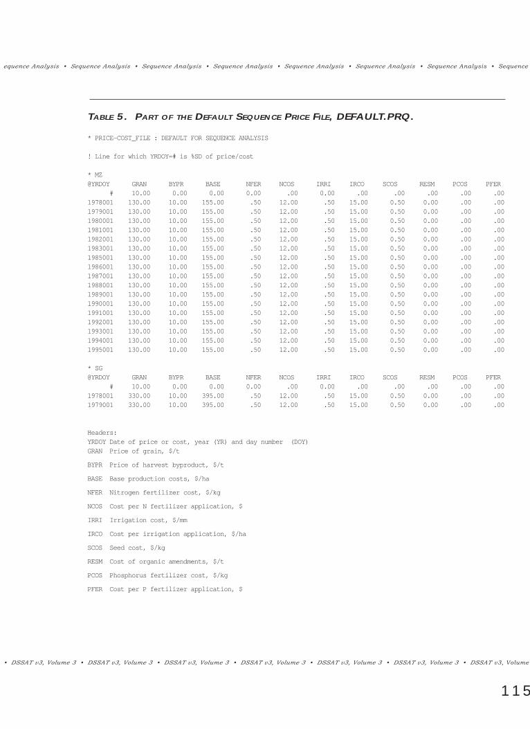
equence Analysis ¥ Sequence Analysis ¥ Sequence Analysis ¥ Sequence Analysis ¥ Sequence Analysis ¥ Sequence Analysis ¥ Sequence Analysis ¥ Sequence
¥ DSSAT v3, Volume 3 ¥ DSSAT v3, Volume 3 ¥ DSSAT v3, Volume 3 ¥ DSSAT v3, Volume 3 ¥ DSSAT v3, Volume 3 ¥ DSSAT v3, Volume 3 ¥ DSSAT v3, Volume
115
TABLE 5. PART OF THE DEFAULT SEQUENCE PRICE FILE, DEFAULT.PRQ.
* PRICE-COST_FILE : DEFAULT FOR SEQUENCE ANALYSIS
! Line for which YRDOY=# is %SD of price/cost
* MZ@YRDOY GRAN BYPR BASE NFER NCOS IRRI IRCO SCOS RESM PCOS PFER
# 10.00 0.00 0.00 0.00 .00 0.00 .00 .00 .00 .00 .001978001 130.00 10.00 155.00 .50 12.00 .50 15.00 0.50 0.00 .00 .001979001 130.00 10.00 155.00 .50 12.00 .50 15.00 0.50 0.00 .00 .001980001 130.00 10.00 155.00 .50 12.00 .50 15.00 0.50 0.00 .00 .001981001 130.00 10.00 155.00 .50 12.00 .50 15.00 0.50 0.00 .00 .001982001 130.00 10.00 155.00 .50 12.00 .50 15.00 0.50 0.00 .00 .001983001 130.00 10.00 155.00 .50 12.00 .50 15.00 0.50 0.00 .00 .001985001 130.00 10.00 155.00 .50 12.00 .50 15.00 0.50 0.00 .00 .001986001 130.00 10.00 155.00 .50 12.00 .50 15.00 0.50 0.00 .00 .001987001 130.00 10.00 155.00 .50 12.00 .50 15.00 0.50 0.00 .00 .001988001 130.00 10.00 155.00 .50 12.00 .50 15.00 0.50 0.00 .00 .001989001 130.00 10.00 155.00 .50 12.00 .50 15.00 0.50 0.00 .00 .001990001 130.00 10.00 155.00 .50 12.00 .50 15.00 0.50 0.00 .00 .001991001 130.00 10.00 155.00 .50 12.00 .50 15.00 0.50 0.00 .00 .001992001 130.00 10.00 155.00 .50 12.00 .50 15.00 0.50 0.00 .00 .001993001 130.00 10.00 155.00 .50 12.00 .50 15.00 0.50 0.00 .00 .001994001 130.00 10.00 155.00 .50 12.00 .50 15.00 0.50 0.00 .00 .001995001 130.00 10.00 155.00 .50 12.00 .50 15.00 0.50 0.00 .00 .00
* SG@YRDOY GRAN BYPR BASE NFER NCOS IRRI IRCO SCOS RESM PCOS PFER
# 10.00 0.00 0.00 0.00 .00 0.00 .00 .00 .00 .00 .001978001 330.00 10.00 395.00 .50 12.00 .50 15.00 0.50 0.00 .00 .001979001 330.00 10.00 395.00 .50 12.00 .50 15.00 0.50 0.00 .00 .00
Headers:YRDOY Date of price or cost, year (YR) and day number (DOY)GRAN Price of grain, $/t
BYPR Price of harvest byproduct, $/t
BASE Base production costs, $/ha
NFER Nitrogen fertilizer cost, $/kg
NCOS Cost per N fertilizer application, $
IRRI Irrigation cost, $/mm
IRCO Cost per irrigation application, $/ha
SCOS Seed cost, $/kg
RESM Cost of organic amendments, $/t
PCOS Phosphorus fertilizer cost, $/kg
PFER Cost per P fertilizer application, $

Sequence Analysis ¥ Sequence Analysis ¥ Sequence Analysis ¥ Sequence Analysis ¥ Sequence Analysis ¥ Sequence Analysis ¥ Sequence Analysis ¥
DSSAT v3, Volume 3 ¥ DSSAT v3, Volume 3 ¥ DSSAT v3, Volume 3 ¥ DSSAT v3, Volume 3 ¥ DSSAT v3, Volume 3 ¥ DSSAT v3, Volume 3 ¥ DSSAT v3, V
116
If you specify a large number (more than three) of stochastic prices and costs, andyour computer is not one of the fastest, the economic analysis program may takea long time to run. Usually it is best to use only a few stochastic prices and costs.
The price-cost file is sectioned by crop as shown in Table 5. You may have differ-ent sections for different sequence components of the same crop; thus MZ1 andMZ2 might share the same set of prices and costs, or you could have two sec-tions, one headed Ò*MZ1Ó and one Ò*MZ2.Ó If no integer is specified with thecrop code, it is assumed to be a general section, and will be used for all compo-nent numbers with that crop code.
OPTION 2. CHOOSE TO INCLUDE/EXCLUDE FALLOW PERIODS IN ANALYSIS
The second option in the Economic Evaluation menu (Screen 25) allows the userto decide whether to include or exclude the effects of fallow periods in the analy-sis. Selecting this option toggles the text from ÒincludeÓ to ÒexcludeÓ or vice-versa. Fallow periods often have some economic cost, and you may want toincorporate these into the analysis. If you include them, then you must have afallow section in the cost-price file you are using.
OPTION 3. EDIT PRICE FILE FOR SENSITIVITY ANALYSIS
When you choose this option in Screen 25, the program loads the default editorand the price file that has been selected. You may then make changes to the pricefile, save it, and exit to the analysis program. The editor that the program willload is the editor specified in the SETUP menu item of the DSSAT Shell (seeVolume 1-3, Hunt et al. 1994, of this book for a description of the SETUP menuitem). You should be careful when making edits in the price file that you pre-serve the format of the file, otherwise you may obtain error messages when theanalysis program tries to read the modified file.
OPTION 4. DO ANALYSIS (CALCULATE ECONOMIC RETURNS)When this option is selected from Screen 25, the program will calculate the mean,standard deviation, maximum and minimum value of net return or gross marginper hectare for each sequence year using the costs and prices specified. The firstset of results are for total returns (Screen 27, on following page), including all thecrop components in the sequence (or excluding fallows, if you have selected thisoption). Once these results have been tabulated, you may want to view thereturns arising from each separate crop component. If so, select <Yes> at thispoint to be presented with tables of returns by crop component.

equence Analysis ¥ Sequence Analysis ¥ Sequence Analysis ¥ Sequence Analysis ¥ Sequence Analysis ¥ Sequence Analysis ¥ Sequence Analysis ¥ Sequence
¥ DSSAT v3, Volume 3 ¥ DSSAT v3, Volume 3 ¥ DSSAT v3, Volume 3 ¥ DSSAT v3, Volume 3 ¥ DSSAT v3, Volume 3 ¥ DSSAT v3, Volume 3 ¥ DSSAT v3, Volume
117
You then have the option to plot some results. The plot menu (Screen 28, below)allows you to do box plots of economic returns by crop component or totalreturns (all crop components included in the analysis). Select the option, ÒBox
F1 (Help) 71440 Mem
DSSAT Version 3.0 Crop Sequencing Analysis
Total Return per Hectare
Mean St.Dev. Min Max
Year 1911
Year 1912
Year 1913
Year 1914
Year 1915
Year 1916
Year 1917
Year 1918
Year 1919
Year 1920
230.04
41.77
85.28
65.05
56.40
74.49
24.89
18.40
47.88
73.33
84.66
73.82
92.87
114.94
95.37
100.17
101.02
89.13
109.34
95.61
102.55
-62.64
-65.55
-95.57
-103.03
-99.50
-113.56
-105.71
-73.25
-103.87
430.76
228.98
229.98
320.76
226.15
246.28
223.78
251.42
313.52
293.66
Press any key to continue..
SCREEN 27.
Modify hardcopy options
About SUSTAIN2 ....
Exit
F1 (Help) 71440 Mem
Main Menu
DSSAT Version 3.0 Crop Sequencing Analysis
Economic Evaluation
Access a price file (current file EBAF1101.PRQ)
Choose to include fallow periods in analysis
Edit price file for sensitivity analysis
Do analysis
Quit ...
Plot Menu
Box Plot of Returns - MZ1
Box Plot of Returns - FA1
Box Plot of Total Returns
Probability Analysis
Review results
Exit economic analysis
SCREEN 28.
71440
71440

Sequence Analysis ¥ Sequence Analysis ¥ Sequence Analysis ¥ Sequence Analysis ¥ Sequence Analysis ¥ Sequence Analysis ¥ Sequence Analysis ¥
DSSAT v3, Volume 3 ¥ DSSAT v3, Volume 3 ¥ DSSAT v3, Volume 3 ¥ DSSAT v3, Volume 3 ¥ DSSAT v3, Volume 3 ¥ DSSAT v3, Volume 3 ¥ DSSAT v3, V
118
Plot of Total Returns,Ó in Screen 28 and the resulting box plot for all years isshown in Screen 29 (below), in the same way as for the biophysical variable boxplots described above.
Return to the plot menu (Screen 28). Select the ÒProbability AnalysisÓ option; theresulting screen is shown as Screen 30 (on following page). Again, you may do aprobability analysis by crop component or for total returns (all components
❇
❇
❇
❇ ❇
❇❇
❇
❇ ❇❇
❇
❇ ❇ ❇❇
❇
❇
❇❇
❇
❇❇
❇
❇❇❇
❇
❇
❇
❇
500.0
400.0
300.0
200.0
100.0
0.0
-100.0
MONEY / HA
BOX PLOT OF MONETARY RETURNS PER HA, ALL
YEAR
1916 1924 1932
ALL_YRS
1908 1940
SCREEN 29.
1916 1924 19321908
ALL

equence Analysis ¥ Sequence Analysis ¥ Sequence Analysis ¥ Sequence Analysis ¥ Sequence Analysis ¥ Sequence Analysis ¥ Sequence Analysis ¥ Sequence
¥ DSSAT v3, Volume 3 ¥ DSSAT v3, Volume 3 ¥ DSSAT v3, Volume 3 ¥ DSSAT v3, Volume 3 ¥ DSSAT v3, Volume 3 ¥ DSSAT v3, Volume 3 ¥ DSSAT v3, Volume
119
together). Select the ÒTotal returnsÓ option. You are then asked to enter a criticalreturn, $/ha, in Screen 31 (below). This might be a threshold value of returnsthat the sequence is required to generate. In some situations, the probability of
F1 (Help) 71440 Mem
DSSAT Version 3.0 Crop Sequencing Analysis
Modify hardcopy options
About SUSTAIN2 ....
Exit
Main MenuEconomic Evaluation
Access a price file (current file EBAF1101.PRQ)
Choose to include fallow periods in analysis
Edit price file for sensitivity analysis
Do analysis
Quit ...
Plot Menu
Box Plot of Returns - MZ1
Box Plot of Returns - FA1
Box Plot of Total Returns
Probability Analysis
Review results
Exit economic analysis
Probability Analysis
Returns -- MZ1
Returns -- FA1
Total returns
SCREEN 30.
F1 (Help) 71440 Mem
DSSAT Version 3.0 Crop Sequencing Analysis
Modify hardcopy options
About SUSTAIN2 ....
Exit
Main MenuEconomic Evaluation
Access a price file (current file EBAF1101.PRQ)
Choose to include fallow periods in analysis
Edit price file for sensitivity analysis
Do analysis
Quit ...
Plot Menu
Box Plot of Returns - MZ1
Box Plot of Returns - FA1
Box Plot of Total Returns
Probability Analysis
Review results
Exit economic analysis
Probability Analysis
Returns -- MZ1
Returns -- FA1
Total returns
Variable : Enter critical return, $/HA
Current Value : .000
Maximum Value : 430.765
Minimum Value : -134.196
New Value : 0.0 ■ ■ ■ ■ ■ ■
SCREEN 31.
71440
71440

Sequence Analysis ¥ Sequence Analysis ¥ Sequence Analysis ¥ Sequence Analysis ¥ Sequence Analysis ¥ Sequence Analysis ¥ Sequence Analysis ¥
DSSAT v3, Volume 3 ¥ DSSAT v3, Volume 3 ¥ DSSAT v3, Volume 3 ¥ DSSAT v3, Volume 3 ¥ DSSAT v3, Volume 3 ¥ DSSAT v3, Volume 3 ¥ DSSAT v3, V
120
failing to generate a certain level of returns from an enterprise is an importantcriterion of viability; if this probability of failure increases through time, then thisraises serious questions concerning the long-term viability of the crop sequenceor rotation. The probability analysis performed is one way of addressing thisissue.
Having selected the critical return (Screen 31; enter a value of $0/ha here), theprogram will calculate the probability each year of failing to meet this criticalreturn. The resulting screen (Screen 32, below) shows the probability of thesequence failing to generate positive returns per hectare in each sequence year.Press any key to complete the display of the table. You are then asked if youwant to plot these probabilities. Enter <Y> to produce the plot in Screen 33 (onfollowing page).
The costs and prices used in the example are hypothetical (and are also constantthroughout the sequence from 1911 to 1940; edit the file EBAF1101.PRQ to seethis). As might be expected in such circumstances, reductions in mean yieldsresult in increased probabilities of negative returns across the years of thesequence.
F1 (Help) 71440 Mem
DSSAT Version 3.0 Crop Sequencing Analysis
Probability of Obtaining < .00 $/Ha
Component Year Probability
ALL
ALL
ALL
ALL
ALL
ALL
ALL
ALL
ALL
ALL
1911
1912
1913
1914
1915
1916
1917
1918
1919
1920
.000
.297
.207
.303
.291
.240
.480
.458
.408
.192
Do you want to plot this (Y/N)?
[NO]
SCREEN 32.
71440 MemPress any key to continue....

equence Analysis ¥ Sequence Analysis ¥ Sequence Analysis ¥ Sequence Analysis ¥ Sequence Analysis ¥ Sequence Analysis ¥ Sequence Analysis ¥ Sequence
¥ DSSAT v3, Volume 3 ¥ DSSAT v3, Volume 3 ¥ DSSAT v3, Volume 3 ¥ DSSAT v3, Volume 3 ¥ DSSAT v3, Volume 3 ¥ DSSAT v3, Volume 3 ¥ DSSAT v3, Volume
121
Press any key, then press <Escape> three times to return to the Analysis MainMenu (Screen 4).
1918 1926 1934
1.000
0.800
0.600
0.400
0.200
PROBABILITY
PROBABILITY PLOT, X< .00
YEAR
(1) ALL_YRS
1910 1942
SCREEN 33.
MO D I F Y HA R D C O P Y OP T I O N S
Select this option in the Sequence Analysis main menu in Screen 4 to change theway in which hardcopies of graphs are produced on your printer or plotter. Thescreen that appears (Screen 34, on following page) lists the current graphics hard-copy options. These are stored in an ASCII file called GRAPH.INI (see Table 6).
1918 1926 1934 1910

Sequence Analysis ¥ Sequence Analysis ¥ Sequence Analysis ¥ Sequence Analysis ¥ Sequence Analysis ¥ Sequence Analysis ¥ Sequence Analysis ¥
DSSAT v3, Volume 3 ¥ DSSAT v3, Volume 3 ¥ DSSAT v3, Volume 3 ¥ DSSAT v3, Volume 3 ¥ DSSAT v3, Volume 3 ¥ DSSAT v3, Volume 3 ¥ DSSAT v3, V
122
The various controller options can be changed from this screen, simply by selectingthe option to change and choosing any of the valid options (thus your printer portmight be LPT2 rather than LPT1). On finishing, you can abandon the changes youhave made, or you can save the changes to the file GRAPH.INI.
Normally, configuration of the graphics program will be carried out through theconfiguration menu in the sequence and seasonal analysis programs. You maywish to edit GRAPH.INI with a text editor, however. The section of GRAPH.INIthat holds configuration data for the graphics program is under the [WMGraf] sec-tion of the INI file. Defaults for plotting are defined in this section, in the formatÒkeyword=Ó followed by a string, integer, or real variable. Specifically, the key-word definitions and possible values are as follows:
gcolor[0..7]: refers to the default color palette for plotting. Values are 0 to 15.interval: number of major divisions on the X and Y axis (Ò-9Ó chooses
Autoscaling)tics: number of tic marks between the major divisions (Ò-9Ó chooses
Autoscaling)driver: an integer value of 0 to 33 is specified. The printer/plotter options
are listed in Table 7.
Modify hardcopy options
About SUSTAIN2 ....
Exit
F1 (Help) 71440 Mem
Main Menu
DSSAT Version 3.0 Crop Sequencing Analysis
Hardcopy
Printer driver : HP LaserJet/DeskJet B&W 150 dpi
Printer port : LPT1:
Orientation : Portrait
X Multiplier : 1.00
Y Multiplier : 1.00
File name : C:\DSSAT3\SEQUENCE\VARAN200.GRA
Save changes and exit
Abandon changes and exit
SCREEN 34.
71440

equence Analysis ¥ Sequence Analysis ¥ Sequence Analysis ¥ Sequence Analysis ¥ Sequence Analysis ¥ Sequence Analysis ¥ Sequence Analysis ¥ Sequence
¥ DSSAT v3, Volume 3 ¥ DSSAT v3, Volume 3 ¥ DSSAT v3, Volume 3 ¥ DSSAT v3, Volume 3 ¥ DSSAT v3, Volume 3 ¥ DSSAT v3, Volume 3 ¥ DSSAT v3, Volume
123
port: 0 for LPT1:, 1 for LPT2:, 2 for COM1:, 3 for COM2:, or 4 for redirec-tion of output to a file
orientation: 0 for portrait or 1 for landscapefontsize: fontsize for labels (1 to 20)xmult: X multiplierymult: Y multiplierfile: name for file output if port=4
The printer types supported by the graphics program are shown in Table 7.
You may also need to be aware that legends for the graphics program are takenfrom a DSSAT3 file called DATA.CDE (see Table 8 and Appendix C to Volume 2-1, Jones et al. 1994, of this book). This lists, among other things, the headers,abbreviations, and definitions of the 35 output variables in the summary modeloutput file that can be analyzed using the seasonal analysis program, in the sec-tion headed by the *SUMMARY keyword.
TABLE 6. SAMPLE SECTION OF GRAPH.INI.
[WMgraf]color0=1color1=15color2=14color3=12color4=15color5=10color6=11color7=13interval=-9tics=-9driver=7port=0orientation=0fontsize=6xmult=1.00ymult=1.00usetics=Yusekeyword=1file=OUTPUT

Sequence Analysis ¥ Sequence Analysis ¥ Sequence Analysis ¥ Sequence Analysis ¥ Sequence Analysis ¥ Sequence Analysis ¥ Sequence Analysis ¥
DSSAT v3, Volume 3 ¥ DSSAT v3, Volume 3 ¥ DSSAT v3, Volume 3 ¥ DSSAT v3, Volume 3 ¥ DSSAT v3, Volume 3 ¥ DSSAT v3, Volume 3 ¥ DSSAT v3, V
124
TABLE 7. PRINTER TYPES SUPPORTED BY THE GRAPHICS PROGRAM.
Driver Number Driver Description
0 Epson 9 Pin 60 x 72 dpi1 Epson 9 Pin 120 x 72 dpi2 Epson 9 Pin 240 x 216 dpi3 Epson 24 Pin 180 x 180 dpi4 Epson 24 Pin 360 x 180 dpi5 Epson 24 Pin 360 x 360 dpi6 HP LaserJet/DeskJet B&W 100 dpi7 HP LaserJet/DeskJet B&W 150 dpi8 HP LaserJet/DeskJet B&W 300 dpi9 HP DeskJet 500C 100 dpi 8 color10 HP DeskJet 500C 150 dpi 8 color11 HP DeskJet 500C 300 dpi 8 color12 HP PaintJet 90 dpi B&W13 HP PaintJet 180 dpi B&W14 HP PaintJet 90 dpi 16 color15 HP PaintJet 180 dpi 8 color16 HP PaintJet 180 dpi 16 color (XL)17 HP ThinkJet 192 dpi18 HP 7475A Plotter A size paper19 HP 7475A Plotter B size paper20 HP 7475A Plotter A4 size paper21 HP 7475A Plotter A3 size paper22 HP 7550 Plotter A size paper23 HP 7550 Plotter B size paper24 HP 7550 Plotter A4 size paper25 HP 7550 Plotter A3 size paper26 HP 7440 Plotter A4 size paper27 HP 7470 Plotter A3 size paper28 HP LaserJet HPGL Mode A size paper29 HP LaserJet HPGL Mode B size paper30 PostScript Printer Courier31 PostScript Printer Helvetica32 PostScript Printer Times33 PostScript Printer Symbol
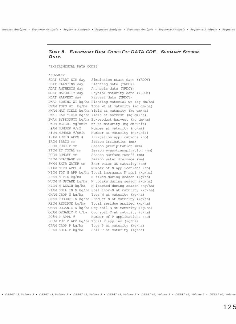
equence Analysis ¥ Sequence Analysis ¥ Sequence Analysis ¥ Sequence Analysis ¥ Sequence Analysis ¥ Sequence Analysis ¥ Sequence Analysis ¥ Sequence
¥ DSSAT v3, Volume 3 ¥ DSSAT v3, Volume 3 ¥ DSSAT v3, Volume 3 ¥ DSSAT v3, Volume 3 ¥ DSSAT v3, Volume 3 ¥ DSSAT v3, Volume 3 ¥ DSSAT v3, Volume
125
TABLE 8. EXPERIMENT DATA CODES FILE DATA.CDE – SUMMARY SECTIONONLY.
*EXPERIMENTAL DATA CODES
*SUMMARYSDAT START SIM day Simulation start date (YRDOY)PDAT PLANTING day Planting date (YRDOY)ADAT ANTHESIS day Anthesis date (YRDOY)MDAT MATURITY day Physiol maturity date (YRDOY)HDAT HARVEST day Harvest date (YRDOY)DWAP SOWING WT kg/ha Planting material wt (kg dm/ha)CWAM TOPS WT. kg/ha Tops wt at maturity (kg dm/ha)HWAM MAT YIELD kg/ha Yield at maturity (kg dm/ha)HWAH HAR YIELD kg/ha Yield at harvest (kg dm/ha)BWAH BYPRODUCT kg/ha By-product harvest (kg dm/ha)HWUM WEIGHT mg/unit Wt at maturity (mg dm/unit)H#AM NUMBER #/m2 Number at maturity (no/m2)H#UM NUMBER #/unit Number at maturity (no/unit)IR#M IRRIG APPS # Irrigation applications (no)IRCM IRRIG mm Season irrigation (mm)PRCM PRECIP mm Season precipitation (mm)ETCM ET TOTAL mm Season evapotranspiration (mm)ROCM RUNOFF mm Season surface runoff (mm)DRCM DRAINAGE mm Season water drainage (mm)SWXM EXTR WATER cm Extr water at maturity (cm)NI#M NITR APPL # Number of N applications (no)NICM TOT N APP kg/ha Total inorganic N appl (kg/ha)NFXM N FIX kg/ha N fixed during season (kg/ha)NUCM N UPTAKE kg/ha N uptake during season (kg/ha)NLCM N LEACH kg/ha N leached during season (kg/ha)NIAM SOIL IN N kg/ha Soil inor-N at maturity (kg/ha)CNAM CROP N kg/ha Tops N at maturity (kg/ha)GNAM PRODUCT N kg/ha Product N at maturity (kg/ha)RECM RESIDUE kg/ha Total residue applied (kg/ha)ONAM ORGANIC N kg/ha Org soil N at maturity (kg/ha)OCAM ORGANIC C t/ha Org soil C at maturity (t/ha)PO#M P APPL # Number of P applications (no)POCM TOT P APP kg/ha Total P applied (kg/ha)CPAM CROP P kg/ha Tops P at maturity (kg/ha)SPAM SOIL P kg/ha Soil P at maturity (kg/ha)

Sequence Analysis ¥ Sequence Analysis ¥ Sequence Analysis ¥ Sequence Analysis ¥ Sequence Analysis ¥ Sequence Analysis ¥ Sequence Analysis ¥
DSSAT v3, Volume 3 ¥ DSSAT v3, Volume 3 ¥ DSSAT v3, Volume 3 ¥ DSSAT v3, Volume 3 ¥ DSSAT v3, Volume 3 ¥ DSSAT v3, Volume 3 ¥ DSSAT v3, V
126
Having analyzed one simulation summary file, you can choose to analyze anoth-er file in Screen 5. If you choose to do so, you have the option to print the sum-mary results file that you have generated during the session for the particularsummary output file. Note that a new analysis results (SQR) file will be pro-duced for each summary output file (SQS) you analyze. A sample of part of thisfile is reproduced in Table 9. This file can be edited as required, and the dataimported into any application capable of reading ASCII text files for whateverpurpose you require.
SE L E C T I N G AN O T H E R IN P U T F I L E F O R AN A LY S I S
IN F O R M AT I O N A N D ER R O R ME S S A G E S
A number of information and error messages are produced by the sequenceanalysis program. In the list that follows, each message is preceded by a single-digit code and a three digit message/error number. If the single-digit code is Ò0,Óthen this is a fatal error, and the program exits. If the code is Ò1,Ó then the pro-gram will continue, as the error may not be fatal. Information messages have codeÒ1Ó also. Some of these messages are self-explanatory. Others are indications ofserious problems, and you should check your file formats.
0 001 Cannot find directory file :The summary output listing file could not be found in the current directory.
0 002 No entries found in file :The summary output listing file could be found, but no valid entries were foundin it.
1 003 Cannot find file :The specified file cannot be found in the appropriate directory.
0 004 Error reading :An error occurred during file reading; this is usually due to incorrect format ofthe specified file.
0 007 Cannot access file :The specified file cannot be found in the appropriate directory.
1 008 Read error in subroutine GETCOD, file :An error occurred in reading the specified file.
0 009 Code could not be found :The program attempted to find the specified code in the DSSATPRO.FLE, butcould not find it. The pathname associated with the code specifies the location ofthe graphics program for the sequence analysis graphics

equence Analysis ¥ Sequence Analysis ¥ Sequence Analysis ¥ Sequence Analysis ¥ Sequence Analysis ¥ Sequence Analysis ¥ Sequence Analysis ¥ Sequence
¥ DSSAT v3, Volume 3 ¥ DSSAT v3, Volume 3 ¥ DSSAT v3, Volume 3 ¥ DSSAT v3, Volume 3 ¥ DSSAT v3, Volume 3 ¥ DSSAT v3, Volume 3 ¥ DSSAT v3, Volume
127
TABLE 9. PART OF SEQUENCE ANALYSIS RESULTS FILE EPAF1101.SQR.
*SQ_ANALYSIS_LOG : EBAF1101SQ
Date: 21 Apr, 1994 Time: 10:45:13
Input file : C:\DSSAT3\SEQUENCE\EBAF1101.SQS —————————-
Analysis of Treatment Number 1
Input File Analysis
Experiment Code : EBAF 11 01Number of runs : 900Number of reps : 15Starting year : 1911Ending year : 1941Runs per rep : 60Runs per rotation: 2
Calculated Values: Variable = HAR YIELD kg/ha MZ1
Year Mean St.Dev1911.0 2223.87 405.991912.0 1087.53 394.241913.0 1401.67 559.151914.0 1242.33 674.781915.0 1206.80 587.821916.0 1323.13 614.011917.0 971.60 621.631918.0 913.87 500.091919.0 1107.20 631.991920.0 1291.93 539.441921.0 595.13 360.271922.0 971.87 588.371923.0 916.47 566.531924.0 853.87 444.651925.0 935.80 363.331926.0 693.20 475.741927.0 1129.73 510.321928.0 304.27 338.101929.0 740.53 500.521930.0 650.47 402.821931.0 694.87 376.091932.0 911.07 485.26

Sequence Analysis ¥ Sequence Analysis ¥ Sequence Analysis ¥ Sequence Analysis ¥ Sequence Analysis ¥ Sequence Analysis ¥ Sequence Analysis ¥
DSSAT v3, Volume 3 ¥ DSSAT v3, Volume 3 ¥ DSSAT v3, Volume 3 ¥ DSSAT v3, Volume 3 ¥ DSSAT v3, Volume 3 ¥ DSSAT v3, Volume 3 ¥ DSSAT v3, V
128
1933.0 478.20 360.781934.0 703.80 540.221935.0 571.47 376.151936.0 657.40 406.531937.0 508.33 476.071938.0 599.80 384.261939.0 384.80 278.991940.0 618.87 356.37
PercentilesYear 0th 10th 25th 50th 75th 90th 100th1911.0 1708.0 1786.2 1903.0 2309.0 2403.0 2761.2 3041.01912.0 517.0 647.2 781.0 1167.0 1298.0 1446.8 1992.01913.0 480.0 606.2 999.0 1748.0 1869.5 1969.6 1987.01914.0 183.0 442.0 791.0 1142.0 1688.5 2082.2 2530.01915.0 132.0 418.0 794.0 1294.0 1594.0 1923.2 1970.01916.0 164.0 521.6 897.5 1346.0 1812.5 2026.6 2102.01917.0 80.0 239.8 531.5 829.0 1563.5 1812.6 1955.01918.0 114.0 432.6 573.5 882.0 1249.0 1296.2 2111.01919.0 400.0 499.0 590.0 911.0 1411.5 1969.2 2467.01920.0 129.0 719.0 965.0 1325.0 1640.5 1763.4 2363.01921.0 109.0 131.0 287.0 669.0 842.0 978.6 1261.01922.0 68.0 251.2 592.5 1098.0 1290.0 1418.8 2370.01923.0 84.0 133.4 588.0 930.0 1226.0 1571.6 2026.01924.0 83.0 247.8 579.0 912.0 1232.5 1393.6 1404.01925.0 129.0 545.0 736.5 1018.0 1130.0 1324.6 1541.01926.0 88.0 131.6 424.0 660.0 831.0 1368.6 1697.01927.0 115.0 581.0 456.5 1264.0 1509.5 1714.2 1917.01928.0 67.0 82.6 90.5 117.0 430.0 783.8 1123.01929.0 68.0 96.0 331.5 740.0 1012.5 1445.2 1552.01930.0 94.0 219.6 496.0 558.0 780.5 1068.6 1704.01931.0 90.0 217.6 417.0 677.0 934.5 1215.2 1280.01932.0 88.0 296.2 605.0 1019.0 1205.0 1476.4 1705.01933.0 36.0 74.2 101.5 527.0 712.0 939.8 1051.01934.0 43.0 96.4 396.0 701.0 911.5 1220.4 2116.01935.0 25.0 89.4 257.0 640.0 748.0 966.6 1338.01936.0 129.0 201.6 421.5 610.0 749.5 1106.0 1693.01937.0 54.0 74.2 100.5 390.0 749.5 1189.6 1488.01938.0 47.0 143.0 415.5 574.0 722.0 1102.8 1447.01939.0 46.0 67.4 89.0 449.0 601.0 694.4 827.01940.0 80.0 117.2 466.0 593.0 811.0 1126.2 1216.0

equence Analysis ¥ Sequence Analysis ¥ Sequence Analysis ¥ Sequence Analysis ¥ Sequence Analysis ¥ Sequence Analysis ¥ Sequence Analysis ¥ Sequence
¥ DSSAT v3, Volume 3 ¥ DSSAT v3, Volume 3 ¥ DSSAT v3, Volume 3 ¥ DSSAT v3, Volume 3 ¥ DSSAT v3, Volume 3 ¥ DSSAT v3, Volume 3 ¥ DSSAT v3, Volume
129
Regression of Means Output
Type = Exponential
constant = 78.2470 gradient = -.0372 r-squared =.6053s yx = 236.041200 SE of gradient = 4.978952T-test of gradient: t = .0075 prob of greater value = .994
Year HAR YIELD kg/ha Residual Estimate
1911. 2223.8670 821.9390 1401.92801912. 1087.5330 -263.2627 1350.79601913. 1401.6670 100.1375 1301.52901914. 1242.3330 -11.7258 1254.05901915. 1206.8000 -1.5211 1208.32101916. 1323.1330 158.8826 1164.25101917. 971.6000 -150.1877 1121.78801918. 913.8666 -167.0073 1080.87401919. 1107.2000 65.7482 1041.45201920. 1291.9330 288.4659 1003.46701921. 595.1334 -371.7352 966.86851922. 971.8666 40.2621 931.60451923. 916.4667 18.8397 897.62701924. 853.8666 -11.0217 864.88841925. 935.8000 102.4562 833.34381926. 693.2000 -109.7501 802.95011927. 1129.7330 356.0688 773.66451928. 304.2667 -441.1804 745.44701929. 740.5333 22.2745 718.25881930. 650.4667 -41.5955 692.06211931. 694.8666 28.0454 666.82121932. 911.0667 268.5660 642.50061933. 478.2000 -140.8671 619.06711934. 703.8000 107.3115 596.48851935. 571.4667 -3.2664 574.73301936. 657.4000 103.6289 553.77111937. 508.3333 -25.2404 533.57371938. 599.8000 85.6870 514.11301939. 384.8000 -110.5623 495.36231940. 618.8666 141.5714 477.2952

Sequence Analysis ¥ Sequence Analysis ¥ Sequence Analysis ¥ Sequence Analysis ¥ Sequence Analysis ¥ Sequence Analysis ¥ Sequence Analysis ¥
DSSAT v3, Volume 3 ¥ DSSAT v3, Volume 3 ¥ DSSAT v3, Volume 3 ¥ DSSAT v3, Volume 3 ¥ DSSAT v3, Volume 3 ¥ DSSAT v3, Volume 3 ¥ DSSAT v3, V
130
1 016 Bad crop code (record #, file):Crop code found in the specified file that is not valid.
1 017 More than 9 crop codes found in fileThe summary output file contained more than 9 crop codes, its current limit.
1 018 Sequence length exceeds 50 yearsThe summary output file is too long to analyze.
0 019 Multiple Treatments Found in File :Two or more sequence treatments were found in the summary output file. Youmust choose which one to analyze.
1 020 A problem was encountered executing another programThe program was not able to execute another program; check the free RAM thatyou have on your computer, and increase it if possible by unloading unnecessaryresident programs (e.g., a network).
1 023 Error in TUKEY.FORAn error occurred when calculating percentiles of a distribution.
1 024 READ Error in file :A read error occurred in the specified file; check the format of the file.
1 026 READ Error in DATA.CDEAn error occurred when reading the file DATA.CDE; check that it is complete andthe format is correct.
1 028 Total number of runs exceeds 1000See message 031.
1 029 Total number of years exceeds 50See message 031.
1 030 Number of replicates exceeds 20See message 031.
1 031 File is too big to analyze:This error message arises in conjunction with one of three other messages, andrefers to the fact that the selected summary output file is too large with respect tototal number of runs (error message 028), number of years (error message 029), ornumber of replicates (error message 030).
1 032 Analysis results written to the file :Analysis results have been written to the specified file.Program output has been written to the specified file.

equence Analysis ¥ Sequence Analysis ¥ Sequence Analysis ¥ Sequence Analysis ¥ Sequence Analysis ¥ Sequence Analysis ¥ Sequence Analysis ¥ Sequence
¥ DSSAT v3, Volume 3 ¥ DSSAT v3, Volume 3 ¥ DSSAT v3, Volume 3 ¥ DSSAT v3, Volume 3 ¥ DSSAT v3, Volume 3 ¥ DSSAT v3, Volume 3 ¥ DSSAT v3, Volume
131
0 038 Error in filename :Error in filename specification.
1 039 Crop code not matched in price file :There was no section in the price file corresponding to the specified crop code;you must edit the file so that this section exists.
1 040 Read error in price file :Check the format of the price file; a read error occurred.
0 041 Cannot find file :Specified file cannot be found.
0 042 Error in :
0 043 Read error in file :Read error in the specified file.
0 044 Must have at least 2 replicates for a CPF plot!
0 046 ERIC2 size problemArray overflow error.
1 047 A price file must be accessed using opt. 1 before using this optionYou must access a price file before attempting to carry out the economic calcula-tions.
1 049 All variances are zero; <Enter> to continue
1 050 Cannot find a file .. choose again :
1 051 You must first select a model output file!Select one of the analysis options before continuing.
1 052 More than 10 treatments found; rest ignoredThe simulation summary output file contains more than 10 treatments; you maychoose one of the first 10 only.
1 053 You must choose a treatment .. or loop forever!!
1 055 Problem in finding the appropriate help screenThe appropriate help screen could not be found.
1 058 There were no matching files found!
1 060 The requested subdirectory to be searched doesnÕt exist!!!

Sequence Analysis ¥ Sequence Analysis ¥ Sequence Analysis ¥ Sequence Analysis ¥ Sequence Analysis ¥ Sequence Analysis ¥ Sequence Analysis ¥
DSSAT v3, Volume 3 ¥ DSSAT v3, Volume 3 ¥ DSSAT v3, Volume 3 ¥ DSSAT v3, Volume 3 ¥ DSSAT v3, Volume 3 ¥ DSSAT v3, Volume 3 ¥ DSSAT v3, V
132
1 070 No valid data;For the crop code(s) and output variable selected, there are no valid data.
1 071 Error in regression routine (divide by zero or inputs out of range)Problem in regression calculations; check the summary output file.
1 072 Reported regression outputs will not be meaningful;Problem in regression.
1 073 Do a regression before plotting!You must do a regression before you can plot the results.
1 074 All residuals are zero
0 075 File DATA.CDE not found
0 076 Error in JNOProblem in counter in summary output file; check its format.
1 077 You must choose at least ONE crop code from this list;
1 078 Multiple crop codes chosen .. Choose method of analysis
1 079 No data found as specifiedNo data could be found for the variable and crop code(s) chosen.
1 080 All data found are zeroNo non-zero data could be found for the variable and crop code(s) chosen.
1 081 Problem in ECONO2Problem in price-cost calculations.
1 082 You may select up to FOUR crop codes with this option
1 082 This is not implemented yet!
1 083 Box plot of total returns NOT available for only one crop!
1 100 Warning!General warning message.
1 131 You MUST turn on the printer now or the program will crash!
1 148 A problem was encountered in trying to print a file!The results file could not be printed successfully.

equence Analysis ¥ Sequence Analysis ¥ Sequence Analysis ¥ Sequence Analysis ¥ Sequence Analysis ¥ Sequence Analysis ¥ Sequence Analysis ¥ Sequence
¥ DSSAT v3, Volume 3 ¥ DSSAT v3, Volume 3 ¥ DSSAT v3, Volume 3 ¥ DSSAT v3, Volume 3 ¥ DSSAT v3, Volume 3 ¥ DSSAT v3, Volume 3 ¥ DSSAT v3, Volume
133
REFERENCES
The Sequence Analysis program is outlined in the following:
Thornton, P.K., G. Hoogenboom, P.W. Wilkens P W and W.T. Bowen. 1994. Acomputer program to analyze multi-season crop model outputs. AgronomyJournal (in press).
A good source of general information on regression is:
Snedecor, G.W. and W.G. Cochran. 1980. Statistical Methods. Iowa StateUniversity Press, Ames, IA.
Other References:
Hunt, L.A., J.W. Jones, P.K. Thornton, G. Hoogenboom, D.T. Imamura, G.Y. Tsujiand U. Singh. 1994. Accessing data, models and application programs. In:Tsuji, G.Y., G. Uehara and S. Balas (eds.). DSSAT v3. Vol. 1-3. University ofHawaii, Honolulu, HI.
Jones, J.W., L.A. Hunt, G. Hoogenboom, D.C. Godwin, U. Singh, G.Y. Tsuji, N.Pickering, P.K. Thornton, W.T. Bowen, K.J. Boote and J.T. Ritchie. 1994. Inputand output files. In: Tsuji, G.Y., G. Uehara and S. Balas (eds). DSSAT v3. Vol.2-1. University of Hawaii, Honolulu, HI.
Thornton, P.K., G. Hoogenboom, P.W. Wilkens and J.W. Jones. 1994a. Seasonalanalysis. In: Tsuji, G.Y., G. Uehara and S. Balas (eds.). DSSAT v3. Vol. 3-1.University of Hawaii, Honolulu, HI.

Sequence Analysis ¥ Sequence Analysis ¥ Sequence Analysis ¥ Sequence Analysis ¥ Sequence Analysis ¥ Sequence Analysis ¥ Sequence Analysis ¥
DSSAT v3, Volume 3 • DSSAT v3, Volume 3 • DSSAT v3, Volume 3 • DSSAT v3, Volume 3 • DSSAT v3, Volume 3 • DSSAT v3, Volume 3 • D
134

equence Analysis ¥ Sequence Analysis ¥ Sequence Analysis ¥ Sequence Analysis ¥ Sequence Analysis ¥ Sequence Analysis ¥ Sequence Analysis ¥ Sequence
¥ DSSAT v3, Volume 3 ¥ DSSAT v3, Volume 3 ¥ DSSAT v3, Volume 3 ¥ DSSAT v3, Volume 3 ¥ DSSAT v3, Volume 3 ¥ DSSAT v3, Volume 3 ¥ DSSAT v3, Volume
135
The main conclusion of this appendix can be stated simply: to obtain relatively sta-ble estimates of output means and variances from replicated sequence experiments,you should use as many replications as possible. In practice, you should always useat least 10, and preferably nearer to 20 (the limit of the program).
Sequence outputs may be very unstable with fewer than 10 replicates. The majorimplication of this is that it will be possible for users to draw erroneous conclusionsfrom insufficiently replicated sequence experiments. It is easy to show this with acomputer program that ÒsimulatesÓ a crop model by drawing a random samplefrom a normal distribution (with mean 6 and standard deviation 1.5) to representyield, does this for 12 ÒyearsÓ in sequence, and replicates this sequence as often asrequired, from 1 to 100. The null hypothesis of NO TREND OVER THE SEQUENCEis thus true.
Results are shown in Figure 3. In the first graph, with a sample size of 100 (100replicates), there is no apparent trend (nor should there be, as there is none), and themaxima and minima of each distribution from one season to the next do not varygreatly. The other graphs show what happens to random samples with fewer andfewer replicates (20, 10, and 5, respectively). It can be seen that the plots becomeprogressively more erratic; note the increasingly variable maxima and minima, andthe highly variable spread of the median. With only 5 replicates we apparently havean upward trend of the median.
The sequence analysis program was written with two main hypotheses in mind:
1. Cropping systems that have some sort of problem will eventually exhibitdecreasing performance levels over time, be it in terms of yields or economicreturns;
2. Some cropping systems will have problems over long periods of time that areexhibited in terms of increases in variability over the sequence.
The analyses included in the program are designed to allow the user to identifythese types of problems. There may be situations where a simple graph of yields
APPENDIX A. THE STABILITY OF OUTPUT VARIABLES FROM
REPLICATED SEQUENCE EXPERIMENTS

Sequence Analysis ¥ Sequence Analysis ¥ Sequence Analysis ¥ Sequence Analysis ¥ Sequence Analysis ¥ Sequence Analysis ¥ Sequence Analysis ¥
DSSAT v3, Volume 3 ¥ DSSAT v3, Volume 3 ¥ DSSAT v3, Volume 3 ¥ DSSAT v3, Volume 3 ¥ DSSAT v3, Volume 3 ¥ DSSAT v3, Volume 3 ¥ DSSAT v3, V
136
over time is sufficient to say with certainty, this is not a viable sequence. Othersituations may not be so cut and dried.
As noted in the introduction to this document, the sequencing capabilities of theDSSAT v3 crop models have not been extensively tested, and this is another rea-son for exhibiting caution with regard to the conclusions you draw from any sim-ulated sequence experiment.
FIGURE 3. “SIMULATED” SEQUENCE OUTPUTS SHOWING INCREASINGLY ERRATICPLOTS AS REPLICATES FALL BELOW 100 (N = 20, 10 AND 5, RESPECTIVELY).
N=100Y
IELD
10
5
01 3 5 7 9 11
YEAR
N=20
YIE
LD
10
5
01 3 5 7 9 11
YEAR
N=5
YIE
LD10
5
01 3 5 7 9 11
YEAR
N=10
YIE
LD
10
5
01 3 5 7 9 11
YEAR
MAXIMUM
MEDIAN
MINIMUM

J.W. HANSEN, N.B. PICKERING, J.W. JONES, C. WELLS, H. CHAN,D.C. GODWIN
VO L U M E 3 -3
WEATHERMAN
UNIVERSITY OF FLORIDA
MASSEY UNIVERSITY, UNIVERSITY OF HAWAII
INTERNATIONAL FERTILIZER DEVELOPMENT CENTER
INTERNATIONAL BENCHMARK SITES NETWORK FOR AGROTECHNOLOGY TRANSFER

WeatherMan ¥ WeatherMan ¥ WeatherMan ¥ WeatherMan ¥ WeatherMan ¥ WeatherMan ¥ WeatherMan ¥ WeatherMan ¥ WeatherMan ¥ WeatherMa
DSSAT v3, Volume 3 ¥ DSSAT v3, Volume 3 ¥ DSSAT v3, Volume 3 ¥ DSSAT v3, Volume 3 ¥ DSSAT v3, Volume 3 ¥ DSSAT v3, Volume 3 ¥ DSSAT v3, V
138

WeatherMan ¥ WeatherMan ¥ WeatherMan ¥ WeatherMan ¥ WeatherMan ¥ WeatherMan ¥ WeatherMan ¥ WeatherMan ¥ WeatherMan ¥ WeatherMan ¥
139
• DSSAT v3, Volume 3 • DSSAT v3, Volume 3 • DSSAT v3, Volume 3 • DSSAT v3, Volume 3 • DSSAT v3, Volume 3 • DSSAT v3, Volume 3 • DSSAT v3,
CHAPTER ONE.INTRODUCTION
Daily weather data are commonly used as input to mathematical models used inwater related projects and agriculture. While the models expect the data to becomplete and reliable, raw data from a weather station, or even a reliable sec-ondary supplier of weather data, are often flawed. Common data problemsinclude format errors, missing data, unreasonable values, data recorded in differ-ent units than needed, and data in an inconvenient format. Often there are nodata available for a specific site, or a particular variable is not in the availableweather record.
IBSNAT has focused on the development of crop models and software tools suchas the DSSAT to aid research and development in agriculture. Available and reli-able weather data are essential for good predictions using these crop models.The IBSNAT project has specified a minimum daily weather data set and formatfor use with the crop models. In DSSAT v2.1, (IBSNAT 1986), the required dailyvariables were solar radiation (MJ/m2/d), maximum temperature (oC) minimumtemperature (oC), and rainfall (mm). An extended DSSAT v2.1 data set includedphotosynthetically active radiation (PAR, mol/m2/d). DSSAT v3 uses the sameminimum weather data set and allows optional variables, such as PAR, dewpoint (oC) and wind speed (m/s). (For a description of DSSAT v3 file formats, seeVolume 2-1, Jones et al. 1994, of this book)
PR O G R A M DE S C R I P T I O N
The WeatherMan program is designed to simplify or automate many of the tasksassociated with handling, analyzing, and preparing weather data for use withcrop models or other simulation software. WeatherMan can be used either as astand-alone package or called from within the DSSAT v3 Shell (for a descriptionof the Shell, see Volume 1-3, Hunt et al. 1994, of this book). WeatherMan has theability to translate both the format and units of daily weather data files, check forerrors on import, and fill-in missing or suspicious values on export. WeatherMancan also generate complete sets of weather data comprising solar radiation, maxi-mum and minimum temperature, rainfall, and photosynthetically active radia-tion. Summary statistics can be computed and reported in tables. The summarystatistics or daily data can be viewed graphically.
WeatherMan is written in Borland Pascal v.7 (Borland, 1993). The user interfacein WeatherMan was developed using the object-oriented Turbo Vision libraries

provided with Borland Pascal and includes standard pull-down menus; dialogboxes with push buttons, input lines, check boxes, radio buttons and scrollingdynamic lists; and context-sensitive, cross-referencing online help. The userinterface functions with both keyboard and mouse.
WeatherMan ¥ WeatherMan ¥ WeatherMan ¥ WeatherMan ¥ WeatherMan ¥ WeatherMan ¥ WeatherMan ¥ WeatherMan ¥ WeatherMan ¥ WeatherMa
DSSAT v3, Volume 3 ¥ DSSAT v3, Volume 3 ¥ DSSAT v3, Volume 3 ¥ DSSAT v3, Volume 3 ¥ DSSAT v3, Volume 3 ¥ DSSAT v3, Volume 3 ¥ DSSAT v3, V
140
SY S T E M RE Q U I R E M E N T S
OV E RV I E W O F FU N C T I O N S
The WeatherManÕs main menu items are: FILE, STATION, IMPORT/ EXPORT,GENERATE, ANALYZE, OUTPUT, AND QUIT. The FILE menu accesses a user-selectable text editor for data entry and correction, accesses the operating system(DOS), and allows the current weather data directory to be changed. A newweather station is selected from the STATION menu. The IMPORT/EXPORTmenu handles the conversion of file formats and units when importing andexporting weather into or from an archive data file. Importing data refers toreading a new weather data file and storing the data in an internal, archive datafile. Exporting data refers to creating a new weather data file and writing datafrom the archive weather data file to a new data file in a prescribed format.WeatherMan checks for and flags format or range errors on import. On export,data flagged as missing or suspect can be replaced with estimates using severalmethods. The GENERATE menu permits generation of synthetic sequences ofsolar radiation, maximum and minimum temperature, rainfall, and photosynthet-ically active radiation for any duration. The ANALYZE menu includes the com-putation of summary statistics and the ability to display the results using tablesor graphs. The OPTIONS menu allows the user to customize and save the cur-rent configuration. The user can terminate a WeatherMan session using QUITfrom the main menu or selecting the option, ÒExit,Ó under the FILE menu.
WeatherMan is designed to run on an IBM compatible PC with DOS v3.1 or laterand with at least 280 kB of available conventional RAM to work with 5 weathervariables. Each additional variable requires about 12 kB of additional RAM.WeatherMan will store its overlay in expanded memory if it is available. It willbe slower without expanded memory and require more conventional memory.We recommend at least 300 kB of available expanded memory when runningWeatherMan. While a math co-processor is not required, it is recommended. Ahard disk is recommended. Archive weather data occupies about 14 kB of diskspace per year for five variables. Standard video drivers are detected automati-cally. Graphs can be output to several printers, plotters, and file formats.

WeatherMan ¥ WeatherMan ¥ WeatherMan ¥ WeatherMan ¥ WeatherMan ¥ WeatherMan ¥ WeatherMan ¥ WeatherMan ¥ WeatherMan ¥ WeatherMan ¥
¥ DSSAT v3, Volume 3 ¥ DSSAT v3, Volume 3 ¥ DSSAT v3, Volume 3 ¥ DSSAT v3, Volume 3 ¥ DSSAT v3, Volume 3 ¥ DSSAT v3, Volume 3 ¥ DSSAT v3, Volume
141
CHAPTER TWO.GETTING STARTED
WeatherMan can be run either from the DSSAT v3 Shell or as a stand-alone pro-gram. From the DSSAT v3 Shell, call the WeatherMan by using the cursor keys toselect the DATA main menu item and then the submenu items, ÒWeatherÓ andthen ÒUtilities.Ó Alternatively, WeatherMan can be called by typing WM fromthe DSSAT3 directory, or from any directory if \DSSAT3 is identified in the DOSPATH variable.
The opening screen of the WeatherMan has a main menu on the top line, a blankdesktop in the center, and a status line on the bottom. An example of the startupscreen appearance is given in Screen 1 (below).
SCREEN 1.
STA RT I N G WE AT H E RMA N
WE AT H E RMA N US E R IN T E R FA C E
The WeatherMan interface is written in Borland PascalÕs Turbo Vision and gener-ally follows the Microsoft Windows protocols. A mouse or a few standard key-strokes are used to access WeatherManÕs features (Table 1).
File Station Import/Export Generate Analyze Options Quit
F1 Help F10 Menu Stn: CCQU
12:35:59

WeatherMan ¥ WeatherMan ¥ WeatherMan ¥ WeatherMan ¥ WeatherMan ¥ WeatherMan ¥ WeatherMan ¥ WeatherMan ¥ WeatherMan ¥ WeatherMa
DSSAT v3, Volume 3 ¥ DSSAT v3, Volume 3 ¥ DSSAT v3, Volume 3 ¥ DSSAT v3, Volume 3 ¥ DSSAT v3, Volume 3 ¥ DSSAT v3, Volume 3 ¥ DSSAT v3, V
142
TABLE 1. USER INTERFACE ITEMS AND THEIR FUNCTIONS IN WEATHERMAN.
Item Function
Main menu Accessed with the <ALT>-hotkey sequence, e.g., <ALT>-<F>,accesses the FILE main menu item. Or press the <F10> keyto select the menu and use the cursor keys.
Menu item Press the hotkey letter or highlight the item using cursorkeys, and use the <ENTER> key or left mouse button. Menuitems (or sub-menus) do not require the <ALT> sequence.
Dialog box A window that prompts for some user response. A dialog boxmay contain push buttons, input lines, input lists, radiobuttons, or check boxes. In general, these items may beselected with a mouse, <TAB>, <SHIFT>-<TAB), or an <ALT>-hotkey combination.
Push button A rectangular button that is activated by a mouse double-click or pressing the <ENTER> key. Most dialog boxes con-tain at-least OK and CANCEL buttons.
Input line A highlighted bar that accepts string or numeric data. Thecursor, <INSERT>, and <DELETE> keys are active in an inputline.
Input list An input line followed by a down arrow icon opens a dialogbox with a list of permissible entries. Activate byselecting the icon with a mouse or selecting the inputline, and pressing the down cursor key.
Radio button Radio buttons, (●), allow you to select one item from a setof options. Select with a mouse, up and down cursor keysand the <SPACE> bar, or an <ALT>-hotkey combination.
Check box Check boxes, i.e., [X], allow you to select any combinationfrom a set of options. Select the same way as radio but-tons.
<F1> Context sensitive help.
CANCEL button Ignores choice and returns to previous menu.
OK button Accepts choice and exits the current dialog box or contin-ues the process.
<ESC> Equivalent to CANCEL.

WeatherMan ¥ WeatherMan ¥ WeatherMan ¥ WeatherMan ¥ WeatherMan ¥ WeatherMan ¥ WeatherMan ¥ WeatherMan ¥ WeatherMan ¥ WeatherMan ¥
¥ DSSAT v3, Volume 3 ¥ DSSAT v3, Volume 3 ¥ DSSAT v3, Volume 3 ¥ DSSAT v3, Volume 3 ¥ DSSAT v3, Volume 3 ¥ DSSAT v3, Volume 3 ¥ DSSAT v3, Volume
143
<ENTER> Accepts highlighted choice and performs function. For mostdialog boxes the default option is OK. For data entry dia-log boxes, pressing the <ENTER> key is equivalent to press-ing the <TAB> key.
L mouse button Left button on the computer mouse. A single click high-lights an item. Double click is equivalent to pressing the<ENTER> key.
R mouse button Right button on the computer mouse. Equivalent to CANCEL.
<TAB> Move to the next data entry cell.
<SHIFT>-<TAB> Move to the previous data entry cell.
<HOME> Move to first data entry cell.
<END> Move to the last data entry cell.
Down arrow Same as using <TAB> key in data entry dialog boxes. Whenan input line shows a down arrow icon, activates history orlist dialog box with choices listed for selection. Thehistory dialog box displays previous selections.
Up arrow Same as using the <SHIFT>-<TAB> keys in data entry dialogboxes.
<CTRL>-right arrow Move to next data column.
<CTRL>-left arrow Move to previous data column.
[■] Click on [■] icon to close dialog box or window. An alter-native to using the <ESC> key or CANCEL button.
<ALT>-<X> Exit /Quit.
<ALT>-<Q> Exit /Quit.

WeatherMan ¥ WeatherMan ¥ WeatherMan ¥ WeatherMan ¥ WeatherMan ¥ WeatherMan ¥ WeatherMan ¥ WeatherMan ¥ WeatherMan ¥ WeatherMa
DSSAT v3, Volume 3 ¥ DSSAT v3, Volume 3 ¥ DSSAT v3, Volume 3 ¥ DSSAT v3, Volume 3 ¥ DSSAT v3, Volume 3 ¥ DSSAT v3, Volume 3 ¥ DSSAT v3, V
144
Where the dialog box displays a Down Arrow (¯) symbol, it is important to dis-tinguish between the <TAB> and Down Arrow keys. The <TAB> and <SHIFT>-<TAB> keys are used for moving around the dialog box without the mouse,while the Down Arrow key activates a history list of previous choices or a list ofavailable choices. An example of a history list is given in Screen 2 (below) for thechoice of a weather input file name.
The previously selected file names are shown in the history list asUFGA7601.WTH, UFGA7801.WTH and UFGA7901.WTH. A file is selected bypressing the <ENTER> key with the name highlighted. Use of history lists helpsspeed up the selection process and avoid typing errors.
[ ]
[ ]
Weather Input File Name
*.*UFGA7901.WTHUFGA7001.WTHUFGA7601.WTH
ALCL5901.WTHATTRIB.FLEAUXSTAT.BIN
CCQU_AHY.SUMCCQU_AMA.SUMCCQU_AMM.SUM
OK
Cancel
SCREEN 2.
CO M M O N DI A L O G BO X E S
A list dialog box is presented when you wish to select a weather station, select afile for import or export, select a file format, or select a file to edit or invert. Anexample of this type of dialog box, for selecting a weather station, is given inScreen 3 (on following page). The file mask on the first line may be restricted forparticular operations. In selecting a weather station, a 4-letter name is expectedand a .CLI extension is automatically appended. Selecting a file for import orexport allows any legal DOS file name and extension. For a format file, any legal

WeatherMan ¥ WeatherMan ¥ WeatherMan ¥ WeatherMan ¥ WeatherMan ¥ WeatherMan ¥ WeatherMan ¥ WeatherMan ¥ WeatherMan ¥ WeatherMan ¥
¥ DSSAT v3, Volume 3 ¥ DSSAT v3, Volume 3 ¥ DSSAT v3, Volume 3 ¥ DSSAT v3, Volume 3 ¥ DSSAT v3, Volume 3 ¥ DSSAT v3, Volume 3 ¥ DSSAT v3, Volume
145
DOS name is accepted and the default extension of .FMT is appended. The ÒFormatNameÓ dialog box has an additional Edit button that is explained in that section inChapter 4. Files from other directories can also be listed by selecting a directory. Anexample of the ÒWeather StationÓ dialog box is given in Screen 3 (below).
Three kinds of archive files for a single station can exist: Raw (or observed), Filled,and Generated. The raw archive file is generally retained, while filled and generat-ed archive files may be automatically deleted upon exiting the WeatherMan,depending on the options selected under the OPTIONS main menu item forÒTemporary filesÓ (see also the section entitled ÒGenerate MenuÓ in Chapter 4). Thearchive file(s) are stored in the climate directory specified in DSSATPRO.FLE or inOPTION\ÓDirectoriesÓ (see Chapter 4).
When an operation (e.g., ÒExport,Ó ÒStatisticsÓ) can be performed on more than onetype of data, an additional dialog box is used to clarify which archive file to use. Anexample of the ÒArchive File TypeÓ dialog box is given in Screen 4 (on followingpage).
For several operations, a time period can be selected. The general form of the ÒTimePeriodÓ dialog box (see Screen 5, on following page) has both starting and ending
[ ] Weather Station
Station name:
Files20032006200820252041250325072508
2509CCFPCCMMCCPACCPOCCQUCCSVFARM
TESTUFGA..\
C:\DSSAT3\WEATHER\CLIMATE\????.CLI2003.CLI 3014 Feb 10, 1994 7:15pm
OK
Cancel
↓
SCREEN 3.
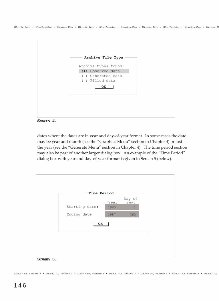
WeatherMan ¥ WeatherMan ¥ WeatherMan ¥ WeatherMan ¥ WeatherMan ¥ WeatherMan ¥ WeatherMan ¥ WeatherMan ¥ WeatherMan ¥ WeatherMa
DSSAT v3, Volume 3 ¥ DSSAT v3, Volume 3 ¥ DSSAT v3, Volume 3 ¥ DSSAT v3, Volume 3 ¥ DSSAT v3, Volume 3 ¥ DSSAT v3, Volume 3 ¥ DSSAT v3, V
146
dates where the dates are in year and day-of-year format. In some cases the datemay be year and month (see the ÒGraphics MenuÓ section in Chapter 4) or justthe year (see the ÒGenerate MenuÓ section in Chapter 4). The time period sectionmay also be part of another larger dialog box. An example of the ÒTime PeriodÓdialog box with year and day-of-year format is given in Screen 5 (below).
Archive File Type
Archive types found: (•) Observed data ( ) Generated data ( ) Filled data
OK
SCREEN 4.
SCREEN 5.
Time Period
Starting date:
Ending date:
Year yearDay of
OK
1
3651987
19801980 1
1987 365

WeatherMan ¥ WeatherMan ¥ WeatherMan ¥ WeatherMan ¥ WeatherMan ¥ WeatherMan ¥ WeatherMan ¥ WeatherMan ¥ WeatherMan ¥ WeatherMan ¥
¥ DSSAT v3, Volume 3 ¥ DSSAT v3, Volume 3 ¥ DSSAT v3, Volume 3 ¥ DSSAT v3, Volume 3 ¥ DSSAT v3, Volume 3 ¥ DSSAT v3, Volume 3 ¥ DSSAT v3, Volume
147
One of the main uses of WeatherMan is to develop complete daily weather datasets from raw data with missing data and incorrect values. Several steps arerequired to complete this process and obtain weather data files that are completeand in the desired format. The minimum requirements for cleaning and refor-matting data are given in Table 2.
ST E P S F O R CL E A N I N G A N D CO N V E RT I N G WE AT H E R
DATA

WeatherMan ¥ WeatherMan ¥ WeatherMan ¥ WeatherMan ¥ WeatherMan ¥ WeatherMan ¥ WeatherMan ¥ WeatherMan ¥ WeatherMan ¥ WeatherMa
DSSAT v3, Volume 3 ¥ DSSAT v3, Volume 3 ¥ DSSAT v3, Volume 3 ¥ DSSAT v3, Volume 3 ¥ DSSAT v3, Volume 3 ¥ DSSAT v3, Volume 3 ¥ DSSAT v3, V
148
TABLE 2. LIST OF ESSENTIAL STEPS FOR CREATING A COMPLETE DAILY WEATHERDATA FILE WITH THE CORRECT FORMAT AND UNITS FROM RAW DATA INWEATHERMAN.
1. Define weather station name and enter site characteristics.
a. Select the menu item Station|Select Station and enter a 4-character code
for the new station.
b. Enter the requested descriptive information for the new station in the
form presented on the screen.
2. Import one or more raw data files.
a. Select the menu item Import/Export and Import Single File items.
b. Create a format definition for the data file that is being imported
when prompted for selecting a file format. Select NEW format and
EDIT buttons to create the format. Enter the requested information
about the format (number of header lines, dates, variable and units
and columns for variables). Then select the SAVE button and give
the defined format a new 4-character name. Usually one would name
the format so that it describes the source of raw data.
c. After saving the format, select OK on the screen and data from the
raw data file will be read into an internal file named Station_GEN.WTD,
where Station_GEN is the name of the weather station.
3. Compute weather generator parameters for the site.
a. Select Generate button, followed by Calculate Parameters.
b. Select the button for Both Sets of Parameters. This will calculate the
necessary parameters for the weather generators so that missing data can
be filled in the exported data file.
4. Export the weather data.
a. Select the Import/Export and Export Yearly Files buttons. Select the
OBSERVED DATA button.
b. When prompted, enter starting and ending dates for the data to be
exported.
c. For exporting daily weather data to be used in DSSAT v3, select the
IBSNAT3 format file. Exported files will normally be located in the directo-
ry C:\DSSAT3\WEATHER and will be named according to the file naming conven-
tions of DSSAT v3 (e.g., ????yy01.WTH, where ???? is the weather station
code and yy is the year).

WeatherMan ¥ WeatherMan ¥ WeatherMan ¥ WeatherMan ¥ WeatherMan ¥ WeatherMan ¥ WeatherMan ¥ WeatherMan ¥ WeatherMan ¥ WeatherMan ¥
¥ DSSAT v3, Volume 3 ¥ DSSAT v3, Volume 3 ¥ DSSAT v3, Volume 3 ¥ DSSAT v3, Volume 3 ¥ DSSAT v3, Volume 3 ¥ DSSAT v3, Volume 3 ¥ DSSAT v3, Volume
149
CHAPTER THREE.INTRODUCTORY TUTORIAL
In this introductory tutorial, you are going to define a new weather station, importweather data and export data to a file of different format. You are also going togenerate data, analyze both data sets and compare them using both tables andgraphs.
In this tutorial, the nomenclature IMPORT/EXPORT|ÓImport single fileÓ means goto the IMPORT/EXPORT menu item of the DSSAT v3 Shell, and then select theÒImport single fileÓ menu item from this menu. Selection is performed by high-lighting the item and pressing the <ENTER> key, or double-clicking on the itemwith the left mouse button, or using the keyboard shortcut keys (i.e., <ALT>-<I>then <S>). Any of the three methods will work. Additional information is given inthe section ÒWeatherMan User InterfaceÓ in Chapter 2.
BR O W S E T H E ME N U A N D ON L I N E HE L P
Pressing the <F1> key provides context-sensitive, cross-referenced help. Look therefirst if questions arise while doing the exercise. Abbreviated help is displayed onthe status line at the bottom of the screen. Pressing the <ESC> key or selecting theCANCEL button will allow you to back out of most processes. Go to the FILE mainmenu item and select ÒAboutÓ (i.e., FILE|ÓAboutÓ). Press the <F1> key to read anintroductory screen describing WeatherMan. Highlight ÒUser interfaceÓ and dou-ble-click or press the <ENTER> key to read about use of the keyboard and mouse.Help for cross-referenced topics can generally be accessed in the same way.
SE L E C T A NE W STAT I O N
Go to the STATION main menu item and open ÒSelect stationÓ (i.e.,STATION|ÓSelect stationÓ). Enter ÒCCQUÓ for the station name. The ÒCCÓ is theID for the institute, CIAT (Centro Internacional de Agricultura Tropical, Cali,Colombia), and the ÒQUÓ is the ID for the station location, Quilichao. When youselect a new (i.e., nonexistent) station, a dialog box, similar to Screen 6 appears,but with default values in each field. The user should enter the values shown inScreen 6 for this example.
NOTE: When the information for a weather station has already been entered, the Screen 6dialog box would not appear the next time that station is selected. ÒCCQUÓ must not beon the distribution disks.

WeatherMan ¥ WeatherMan ¥ WeatherMan ¥ WeatherMan ¥ WeatherMan ¥ WeatherMan ¥ WeatherMan ¥ WeatherMan ¥ WeatherMan ¥ WeatherMa
DSSAT v3, Volume 3 ¥ DSSAT v3, Volume 3 ¥ DSSAT v3, Volume 3 ¥ DSSAT v3, Volume 3 ¥ DSSAT v3, Volume 3 ¥ DSSAT v3, Volume 3 ¥ DSSAT v3, V
150
Select STATION|ÓEdit monthly means.Ó The Ò-99Ó indicates a missing value.Select the CANCEL button or press the <ESC> key to return to the main menu.
Go to IMPORT/EXPORT|ÓImport single file.Ó Import the file, CCQU1980.DATby selecting it from the list. Since the format of CCQU1980.DAT does not matchany of the format files distributed with WeatherMan, you will need to create anew format definition file. You will be asked for a format. Type or highlightNEW and select the EDIT button. Screen 7 (on following page), the ÒEdit FileFormatÓ dialog box, will be presented. Select the VIEW FILE button in Screen 7to view the imported file. The ÒFile ViewerÓ dialog box will be presented withthe file CCQU1980.DAT in the viewer. Note the number of header lines in the filepresented, and the starting position and width (in characters) of the data field foreach variable. You can select variable names and units from lists by selecting thedown arrow icon or by highlighting an input line and pressing the down cursorkey. When you have entered the format information in the Viewer, the ÒEdit FileFormatÓ dialog box should look like Screen 7.
Select the SAVE FORMAT button and save the format as ÒCCQU.Ó Then proceedwith importing by selecting the OK button. If you have enabled the ÒPreview
IM P O RT DA I LY WE AT H E R F I L E S
[ ] Station Data
Location: Quilichao,NorthCauca,Colombia
Latitude (degrees):Longitute (degrees):Elevation (m):Angstrom coefficient A:Angstrom coefficient B:Reference height (m):Wind reference height (m):Mean annual temperature (°C):Temperature amplitude (°C):Start of growing season (day):Duration of growing season (days):
3.080-76.520990.00.250.502.004.0024.00.51
365
OK Cancel
SCREEN 6.

WeatherMan ¥ WeatherMan ¥ WeatherMan ¥ WeatherMan ¥ WeatherMan ¥ WeatherMan ¥ WeatherMan ¥ WeatherMan ¥ WeatherMan ¥ WeatherMan ¥
¥ DSSAT v3, Volume 3 ¥ DSSAT v3, Volume 3 ¥ DSSAT v3, Volume 3 ¥ DSSAT v3, Volume 3 ¥ DSSAT v3, Volume 3 ¥ DSSAT v3, Volume 3 ¥ DSSAT v3, Volume
151
FormatsÓ option under ÒImport Options,Ó you will be presented with a ÒFormatPreviewÓ dialog box, similar to the one shown in Screen 20.
Now import the rest of the files as a group using the CCQU format that you justcreated.
Go to IMPORT/EXPORT|ÓImport multiple filesÓ to import the rest of the files asa group, using the ÒCCQUÓ format that you just created. To do this, select ÒAddGroupÓ in the dialog box presented. Enter the file mask, CCQU*.DAT. You willthen be asked to select a format for the group of files being imported. Afterselecting the format from the list presented when the SELECT FORMAT button ispressed, a listing of files, as shown in Screen 8 (on following page), which matchthe CCQU*.DAT mask, will appear in Screen 8.
Select the OK button to import all of the files in the list. You will then be asked ifyou want to calculate monthly means. Select ÒNoÓ since you will do that in thenext step.
File Station Import/Export Generate Analyze Options Quit 14:39:35
Edit File Format[ ]Header output option: ( ) None ( ) IBSNAT v.3 ( ) IBSNAT v.2 ( ) Variable names ( ) From header file
2
Format name: CCQU
1980 1 1
169
422
Date: Year Month Day
First Position Length
No. header lines:
123456
Variable Units Pos.TMAXTMINRAINSUNH
°F°FinchHrs
33261220 0 0
555400
789101112
000000
000000
↓↓↓↓↓↓
↓↓↓↓↓↓
↓↓↓↓↓↓
↓↓↓↓↓↓
UnitsVariableLen. Len.Pos.
OK Cancel View file Save format
SCREEN 7.

WeatherMan ¥ WeatherMan ¥ WeatherMan ¥ WeatherMan ¥ WeatherMan ¥ WeatherMan ¥ WeatherMan ¥ WeatherMan ¥ WeatherMan ¥ WeatherMa
DSSAT v3, Volume 3 ¥ DSSAT v3, Volume 3 ¥ DSSAT v3, Volume 3 ¥ DSSAT v3, Volume 3 ¥ DSSAT v3, Volume 3 ¥ DSSAT v3, Volume 3 ¥ DSSAT v3, V
152
Go to GENERATE|ÓCalculate parameters,Ó to calculate parameters for both theWGEN and SIMMETEO weather generators. Use the <F1> key to see the differ-ences between WGEN and SIMMETEO. For a more complete description of thesetwo generators, see the section ÒGenerate MenuÓ in this Chapter .
Go to STATION|ÓEdit monthly meansÓ to view the monthly means which areused as parameters for SIMMETEO. The WGEN parameters cannot be viewed oredited directly from WeatherMan. They are, however, saved in a file (CCQU.CLIin the climate directory) and can be edited from the DSSAT v3 Shell (see Volume1-3, Hunt et al. 1994, of this book for a description of the Shell).
GE N E R AT E WE AT H E R DATA
Go to GENERATE|ÓGenerate data.Ó Select SIMMETEO and simulate data for thesame period of time as the data that you imported. This period of time becomesthe defaults in the ÒGenerate Weather DataÓ dialog box (Screen 30).
Files To Import[ ]
Weather fileCCQU1980.DAT
FormatCCQU
CCQU1981.DAT CCQUCCQU1982.DAT CCQUCCQU1983.DAT CCQUCCQU1984.DAT CCQUCCQU1985.DAT CCQU
Add file
Remove file
Select format
Add Group
Cancel
OK
SCREEN 8.
CA L C U L AT E WE AT H E R GE N E R AT O R PA R A M E T E R S

WeatherMan ¥ WeatherMan ¥ WeatherMan ¥ WeatherMan ¥ WeatherMan ¥ WeatherMan ¥ WeatherMan ¥ WeatherMan ¥ WeatherMan ¥ WeatherMan ¥
¥ DSSAT v3, Volume 3 ¥ DSSAT v3, Volume 3 ¥ DSSAT v3, Volume 3 ¥ DSSAT v3, Volume 3 ¥ DSSAT v3, Volume 3 ¥ DSSAT v3, Volume 3 ¥ DSSAT v3, Volume
153
Go to ANALYZE|ÓStatistics.Ó Select all statistics types and time groupings bychecking all of the boxes, using a mouse or cursor keys and press the <SPACE>bar. Then, select the OK button to calculate statistics. Go toANALYZE|ÓReportÓ to view the statistics files. Print only the monthly summa-ry moments file. Highlight the appropriate items in the ÒSummary StatisticsÓ orÒView/Print StatisticsÓ dialog box (see Screen 32 or Screen 33, respectively, inChapter 4) and use the <F1> key if you need help understanding a statistic typeor time grouping.
CA L C U L AT E STAT I S T I C S
CA L C U L AT E STAT I S T I C S F O R T H E GE N E R AT E D DATA
GR A P H OB S E RV E D DA I LY TE M P E R AT U R E
Go again to ANALYZE|ÓStatistics.Ó Select ÒOnly momentsÓ under Type ofStatistic, and ÒOnly Monthly SummaryÓ under Grouping. When you are askedfor the type of archive file, select ÒGenerated data.Ó View and print the results forthe generated data. (NOTE: Check the file header to make sure it is statistics for gener-ated, not observed data.)
123456
Time Plot Ranges[ ]
PlotNum.
[X][X][X][X][X][X]
CCQU RAW ↓CCQU RAW ↓CCQU RAW ↓CCQU RAW ↓CCQU RAW ↓CCQU RAW ↓
Station VariableTMAXTMINRAINSUNH
↓↓↓↓↓↓
Type
Grouping
Range
Graph
Cancel
SCREEN 9.
Go to ANALYZE|ÓGraph.Ó Screen 9 (below) is presented. The initial defaultplots are always daily time series for observed data. Select the plot ranges withminimum and maximum temperature (TMIN and TMAX) by checking the checkboxes at the left, using the <TAB> key and <SPACE> bar. Disable all other plotranges in Screen 9.

WeatherMan ¥ WeatherMan ¥ WeatherMan ¥ WeatherMan ¥ WeatherMan ¥ WeatherMan ¥ WeatherMan ¥ WeatherMan ¥ WeatherMan ¥ WeatherMa
DSSAT v3, Volume 3 ¥ DSSAT v3, Volume 3 ¥ DSSAT v3, Volume 3 ¥ DSSAT v3, Volume 3 ¥ DSSAT v3, Volume 3 ¥ DSSAT v3, Volume 3 ¥ DSSAT v3, V
154
To view the graph, select the GRAPH button. If the graph is cluttered, you canplot a specified range of dates by selecting the RANGE button. Print the graphby pressing the <P> key while the graph is displayed. (Printing will take severalminutes.) Pressing the <G> key toggles the grid lines on or off. Press any otherkey to return to Screen 9.
GR A P H STAT I S T I C S F O R OB S E RV E D A N D GE N E R AT E D
DATA
123456
Time Plot Ranges[ ]
PlotNum.
[X][ ][ ][ ][ ][ ]
CCQU RAW ↓CCQU RAW ↓CCQU RAW ↓CCQU RAW ↓CCQU RAW ↓CCQU RAW ↓
Station VariableTMAXTMINRAINSUNH
↓↓↓↓↓↓
Type
Grouping
Range
Graph
Cancel
Select from List[ ]
Select Site
CCQU: Generated data
CCQU GENCCQU RAW Select
Cancel
SCREEN 10.
As an example graph, we will compare monthly means for maximum daily tem-perature for observed and generated data, and for wet days and dry days. In thescreen presented (Screen 9) when ANALYZE|ÓGraphÓ is selected, press theGROUPING button and then the ÒMonthly summaryÓ time grouping. Highlightthe station for the first plot range and use the down arrow icon to select statisticsfor generated data (CCQU GEN) from the list as shown in Screen 10 (below).
When Screen 11 (on following page) is presented, move to the field underÒVariableÓ in Plot Num. 1 and select mean maximum temperature (TMAX Mean)from the list of available variables in the same way that you selected the station.Finally, move to the field under ÒWet StateÓ and select DRY. Repeat the processfor the next 3 plot ranges. For Plot Num. 2, specify TMAX Mean on WET days

WeatherMan ¥ WeatherMan ¥ WeatherMan ¥ WeatherMan ¥ WeatherMan ¥ WeatherMan ¥ WeatherMan ¥ WeatherMan ¥ WeatherMan ¥ WeatherMan ¥
¥ DSSAT v3, Volume 3 ¥ DSSAT v3, Volume 3 ¥ DSSAT v3, Volume 3 ¥ DSSAT v3, Volume 3 ¥ DSSAT v3, Volume 3 ¥ DSSAT v3, Volume 3 ¥ DSSAT v3, Volume
155
123456
Time Plot Ranges[ ]
PlotNum.
[X][X][X][X][ ][ ]
CCQU GEN ↓CCQU GEN ↓CCQU RAW ↓CCQU RAW ↓CCQU RAW ↓CCQU RAW ↓
Station VariableTMAX MEANTMAX MEANTMAX MEANTMAX MEAN
↓↓↓↓↓↓
Type
Grouping
Range
Graph
Cancel
DRY ↓WET ↓DRY ↓WET ↓ALL ↓ALL ↓
WetState
SCREEN 11.
for generated data. For Plot Num. 3 and 4, specify TMAX Mean on DRY daysand WET days for raw data. After you have specified the four plot ranges, thedialog box will look like Screen 11 (above).
Graph and print the results. Note the similarity between observed and generatedmaximum temperatures and the effect that rain (i.e. WET vs. DRY state) has onmaximum temperature.
EX P O RT DA I LY WE AT H E R F I L E S
Go to IMPORT/EXPORT|ÓExport yearly files.Ó Select the predefined DSSAT v3format file. Single-year files will be named automatically using a default namingconvention. For this example, the first file exported will be calledCCQU8001.WTH, containing data for 1980. Use FILE|ÓEditÓ to access an exter-nal editor to view the newly created CCQU8001.WTH. Also view the original filethat you imported (CCQU1980.DAT) and note the changes in format and units.
You are now familiar with the basic features of WeatherMan. Additional detailson each menu in the WeatherMan main menu screen are described in Chapter 4.

WeatherMan ¥ WeatherMan ¥ WeatherMan ¥ WeatherMan ¥ WeatherMan ¥ WeatherMan ¥ WeatherMan ¥ WeatherMan ¥ WeatherMan ¥ WeatherMa
DSSAT v3, Volume 3 ¥ DSSAT v3, Volume 3 ¥ DSSAT v3, Volume 3 ¥ DSSAT v3, Volume 3 ¥ DSSAT v3, Volume 3 ¥ DSSAT v3, Volume 3 ¥ DSSAT v3, V
156

WeatherMan ¥ WeatherMan ¥ WeatherMan ¥ WeatherMan ¥ WeatherMan ¥ WeatherMan ¥ WeatherMan ¥ WeatherMan ¥ WeatherMan ¥ WeatherMan ¥
¥ DSSAT v3, Volume 3 ¥ DSSAT v3, Volume 3 ¥ DSSAT v3, Volume 3 ¥ DSSAT v3, Volume 3 ¥ DSSAT v3, Volume 3 ¥ DSSAT v3, Volume 3 ¥ DSSAT v3, Volume
157
CHAPTER FOUR.WEATHERMAN REFERENCE GUIDE
F I L E ME N U
WeatherMan works with a specific set of daily weather variables (Table 3). Theset of variables, default range check values (minimum, maximum and maximumdaily change), associated units, and unit conversion factors (multiplier and offset)are specified in a file, called WM.VAR. Variables are stored in their default unitsin the archive files. If you wish to add or change variables or units, please con-tact the authors for assistance.
VA R I A B L E S
The FILE menu item found on the WeatherMan main menu gives access to aneditor, DOS functions, and additional help. The FILE pull-down menu is shownin Screen 12 (below) and its options are described as follows.
EDIT
The ÒEditÓoption accesses a text editor so that data files can be viewed and edit-ed. The user can use his/her own editor by changing the default under theOPTIONS|ÓDirectoriesÓ menus.
File Station Import/Export Generate Analyze Options Quit 14:55:44
EditInvert
Change dir.DOS shell
About
Exit Alt-X
SCREEN 12.

WeatherMan ¥ WeatherMan ¥ WeatherMan ¥ WeatherMan ¥ WeatherMan ¥ WeatherMan ¥ WeatherMan ¥ WeatherMan ¥ WeatherMan ¥ WeatherMa
DSSAT v3, Volume 3 ¥ DSSAT v3, Volume 3 ¥ DSSAT v3, Volume 3 ¥ DSSAT v3, Volume 3 ¥ DSSAT v3, Volume 3 ¥ DSSAT v3, Volume 3 ¥ DSSAT v3, V
158
TABLE 3. WEATHERMAN VARIABLES AND ASSOCIATED UNITS.
Variable Description Default Other
unit units
SRAD Total daily solar radiation MJ/m2 cal/cm2, W-h/m2
TMAX Maximum daily air temperature °C °F, °K
TMIN Minimum daily air temperature °C °F, °K
RAIN Total daily precipitation mm cm, inch
DEWP Dew point temperature or vapor °C °F, °K, Pa, kPa,
pressure MPa, mbar, bar
WIND Total daily wind run km Miles, m/s,
Knots
SUNH Total daily sunshine hours %Hrs n/N, Hrs
PAR Total daily photosynthetic Mol/m2
radiation
TDRY Dry bulb air temperature at 9 am °C °F, °K
TWET Wet bulb air temperature at 9 am °C °F, °K
EVAP Total daily pan evaporation mm cm, inch

WeatherMan ¥ WeatherMan ¥ WeatherMan ¥ WeatherMan ¥ WeatherMan ¥ WeatherMan ¥ WeatherMan ¥ WeatherMan ¥ WeatherMan ¥ WeatherMan ¥
¥ DSSAT v3, Volume 3 ¥ DSSAT v3, Volume 3 ¥ DSSAT v3, Volume 3 ¥ DSSAT v3, Volume 3 ¥ DSSAT v3, Volume 3 ¥ DSSAT v3, Volume 3 ¥ DSSAT v3, Volume
159
INVERT
The ÒInvertÓ option is a utility that reverses the order of lines in a text file(required for the output of some dataloggers which record in reverse chronologi-cal order).
CHANGE DIR.The ÒChange dir.Ó menu option will change the current directory to anotherweather data directory. The ÒChange DirectoryÓ dialog box is given in Screen 13(below).
Change Directory[ ]
Directory nameC:\DSSAT3\WEATHER
Directory treeDrives C:\ DSSAT3 WEATHER CLIMATE
↓
OK
Chdir
Revert
SCREEN 13.
The dialog box shown in Screen 13 applies to the data directory, where the dailyweather data files are kept. The CHDIR button will change the directory tree todisplay the directories below the one that is highlighted. The REVERT buttonrestores the tree to the one presented on entry into the dialog box. The OK buttonaccepts the highlighted directory as the new data directory. The down arrow onthe first line activates the history list of previously chosen data directories. TheÒChange dir.Ó menu option is equivalent to changing the weather data directoryunder the OPTIONS|ÓDirectoriesÓ menus.
DOS SHELL
Selecting the ÒDos shellÓ menu option allows you to leave the WeatherMan pro-gram temporarily, without removing the program from the computerÕs RAM.

WeatherMan ¥ WeatherMan ¥ WeatherMan ¥ WeatherMan ¥ WeatherMan ¥ WeatherMan ¥ WeatherMan ¥ WeatherMan ¥ WeatherMan ¥ WeatherMa
DSSAT v3, Volume 3 ¥ DSSAT v3, Volume 3 ¥ DSSAT v3, Volume 3 ¥ DSSAT v3, Volume 3 ¥ DSSAT v3, Volume 3 ¥ DSSAT v3, Volume 3 ¥ DSSAT v3, V
160
This function is useful for performing DOS functions like RENAME, DELETE orCOPY files. When you have finished any of these functions and wish to return tothe WeatherMan program, type EXIT at the DOS prompt.
ABOUT
The ÒAboutÓ option displays additional information about the WeatherMan pro-gram. The opening screen gives the credits. Introductory information about theprogram can be accessed by pressing the <F1> key from the ÒAboutÓ dialog boxpresented when ÒAboutÓ is selected.
EXIT
The ÒExitÓ option allows you to exit the Weatherman program. You may also exitby pressing the <ALT>-< X> keys.
STAT I O N ME N U
The STATION menu allows you to select a weather station and get general andclimate information for the station. Most operations in WeatherMan require theselection of a weather station name. Two permanent files, located in the climatedirectory, are identified by the station name. A climate file (.CLI) containsdescriptive information about the site, monthly weather generator coefficients,range check values and counts of valid and flagged data. The format of the cli-mate files is given in Appendix B. The station name also identifies an archive file(.WTD) that has a standard format and set of units; this is required by most of thefunctions in WeatherMan (e.g., data checking, data-fill, weather generators, statis-tics, graphics). The archive file is also used for storage of imported data. If theuser only wants to convert data file formats or change units of the variables usingthe ÒConvertÓ option under the IMPORT/EXPORT main menu item, then a per-manent archive file is not retained. The STATION pull-down menu window isdisplayed in Screen 14 (on following page).
In Screen 14, after a weather station has been selected, the 4-letter station ID codeis displayed on the first line of the menu window and also on the status line atthe bottom of the screen. The example station ID code is ÒUFGAÓ in Screen 14.The menu options in the STATION menu are described as follows.
SELECT STATION:The ÒSelect station:Ó option shown in Screen 14 displays a list of all climate (CLI)files in the climate directory. This dialog box uses the ÒFile ListÓ dialog box but

WeatherMan ¥ WeatherMan ¥ WeatherMan ¥ WeatherMan ¥ WeatherMan ¥ WeatherMan ¥ WeatherMan ¥ WeatherMan ¥ WeatherMan ¥ WeatherMan ¥
¥ DSSAT v3, Volume 3 ¥ DSSAT v3, Volume 3 ¥ DSSAT v3, Volume 3 ¥ DSSAT v3, Volume 3 ¥ DSSAT v3, Volume 3 ¥ DSSAT v3, Volume 3 ¥ DSSAT v3, Volume
161
SCREEN 14.
only allows a 4-letter station name. Selecting the OPTIONS main menu item andthen the ÒUpdateÓ option after selecting the station from this menu, places theselected station name in the programÕs configuration file and automatically loadsit the next time WeatherMan is started.
Whenever a new weather station is selected, the user is requested to input generalinformation regarding the new station. These data items are listed in Table 4along with an explanation of each item. Please note that the stationÕs latitude isabsolutely essential.
EDIT STATION INFORMATION
When the ÒEdit station informationÓ option is selected in Screen 14, the ÒStationDataÓ dialog box (see Screen 15, on second following page) for entering additionaldata or editing existing data is presented.
EDIT MONTHLY MEANS
When a new station is selected, a user may select the ÒEdit monthly meansÓoption in order to enter the monthly means of the weather variables for this sta-tion. An example of a ÒMonthly Means and RainfallÓ data entry dialog box isgiven in Screen 16 (on second following page)
Although you do not need to enter the monthly means of the variables listed inScreen 16, many of the options for generating data filling in missing data during
File Station Import/Export Generate Analyze Options Quit 12:16:49
Select station: UFGA
Edit station informationEdit monthly meansCalculate monthly means
F1 Help Stn: UFGA | Select or input a weather station ID.

WeatherMan ¥ WeatherMan ¥ WeatherMan ¥ WeatherMan ¥ WeatherMan ¥ WeatherMan ¥ WeatherMan ¥ WeatherMan ¥ WeatherMan ¥ WeatherMa
DSSAT v3, Volume 3 ¥ DSSAT v3, Volume 3 ¥ DSSAT v3, Volume 3 ¥ DSSAT v3, Volume 3 ¥ DSSAT v3, Volume 3 ¥ DSSAT v3, Volume 3 ¥ DSSAT v3, V
162
TABLE 4. WEATHER STATION INFORMATION REQUIRED FOR A NEW STATION.
Latitude (degrees) Station latitude (+=N, -=S).
Longitude (degrees) Station longitude (+=E, -=W).
Elevation (m) Station elevation above mean sea level.
Angstrom coefficient A Coefficient A in equation: SRAD = (A + B *n/N) * RE, where RE is extraterrestrial radia-tion and n is duration of bright sunshine, andN is daylength.
Angstrom coefficient B Coefficient B in equation: SRAD = (A + B *n/N) * RE.
Reference height (m) Height of meteorological sensors above ground.
Wind reference height (m) Height of anemometer above ground.
Mean annual temperature (°C) Mean annual average daily temperature.
Temperature amplitude (°C) Half the range of monthly means for averagedaily temperature.
Start of growing season (d) Mean day-of-year for last frost.
Duration growing season (d) Mean time from last frost to first frost.
Export will be dis-abled until it has been completed. An alternative to manualdata entry is to calculate the means from the daily data in the raw archive file.Monthly climate statistics are available from several secondary data sources (eg.Conway, et al., 1963; NOAA, 1974; Rudloff, 1981). The last two items in the dia-log box shown in Screen 16 allow you to document the data source and the datacollection period.
CALCULATE MONTHLY MEANS
The ÒCalculate monthly meansÓ option in Screen 14 allows you to computemeans from the data in the raw archive file. This is a reasonable option if thereare sufficient reliable data in the archive file or if there are no available climatedata. The user is given a warning message if there are less than five years of reli-able data in the archive file. Calculating monthly means is equivalent to estimat-ing the SIMMETEO parameters from the Generate menu (see the ÒGenerateMenuÓ section in this Chapter). The ÒCalculate monthly meansÓ option willoverwrite manually-entered data.

WeatherMan ¥ WeatherMan ¥ WeatherMan ¥ WeatherMan ¥ WeatherMan ¥ WeatherMan ¥ WeatherMan ¥ WeatherMan ¥ WeatherMan ¥ WeatherMan ¥
¥ DSSAT v3, Volume 3 ¥ DSSAT v3, Volume 3 ¥ DSSAT v3, Volume 3 ¥ DSSAT v3, Volume 3 ¥ DSSAT v3, Volume 3 ¥ DSSAT v3, Volume 3 ¥ DSSAT v3, Volume
163
SCREEN 15.
File Station Import/Export Generate Analyze Options Quit 12:51:39
Monthly Means and Rainfall--mean monthly values--
123456789101112
10.913.417.221.422.320.820.318.816.614.612.09.9
19.321.224.328.030.932.533.132.931.628.624.521.5
5.77.210.013.517.120.621.921.920.616.311.57.9
94.2118.3109.878.7101.1165.9175.1201.9136.256.959.369.3
8.78.38.35.87.912.416.516.211.36.56.06.8
-99.0-99.0-99.0-99.0-99.0-99.0-99.0-99.0-99.0-99.0-99.0-99.0
0.2500.2500.2500.2500.2500.2500.2500.2500.2500.2500.2500.250
0.5000.5000.5000.5000.5000.5000.5000.5000.5000.5000.5000.500
[ ]
Source:Calculated_from_daily_data 1st year: 1980 No. years: 25
F1 Help Stn: UFGA | Mean solar radiation (MJ/m2/d) for month.
(MJ/m2) (°C) (°C) (mm) days (%) (Y-int) (slope)SPRAD TMAX TMIN rain of wet SUNH A B
Total Number Mean Angstrom coef.
Mon
OK Cancel
SCREEN 16.
[ ] Station Data
Location: Gainesville,Florida
Latitude (degrees):Longitute (degrees):Elevation (m):Angstrom coefficient A:Angstrom coefficient B:Reference height (m):Wind reference height (m):Mean annual temperature (°C):Temperature amplitude (°C):Start of growing season (day):Duration of growing season (days):
29.630-82.370
10.00.250.501.003.0020.97.51
365
OK Cancel
Monthly mean hours of bright sunshine and Angstrom coefficients (Prescott,1940) are included to aid in the estimation of missing daily solar radiation data

WeatherMan ¥ WeatherMan ¥ WeatherMan ¥ WeatherMan ¥ WeatherMan ¥ WeatherMan ¥ WeatherMan ¥ WeatherMan ¥ WeatherMan ¥ WeatherMa
DSSAT v3, Volume 3 ¥ DSSAT v3, Volume 3 ¥ DSSAT v3, Volume 3 ¥ DSSAT v3, Volume 3 ¥ DSSAT v3, Volume 3 ¥ DSSAT v3, Volume 3 ¥ DSSAT v3, V
164
where daily hours of bright sunshine (SUNH) are available. If SUNH data arenot available in the archive file, ÒCalculate monthly meansÓ will use theAngstrom coefficients entered in the ÒStation DataÓ dialog box as defaults (seeScreen 15). If SUNH is available but daily radiation (SRAD) is not, then monthlyAngstrom coefficients will be estimated by the relationship proposed by Rietveld(1978). If sufficient (>5yr) records with both SRAD and SUNH are found for amonth, then Angstrom coefficients will be calculated for that month directly bylinear regression.
IM P O RT/EX P O RT ME N U
The IMPORT/EXPORT menu item found on the WeatherMan main menu allowsyou to perform all the necessary data manipulation for inserting data into anarchive file and extracting it into other files. The IMPORT/EXPORT pull-downmenu is shown in Screen 17 (below) and its options are described as follows.
FILE FORMATS
The ÒFile formatÓ option allows you to define the format of the target weatherdata file to be imported or the destination file to be exported. These formats aresaved in files with .FMT extensions. For example, format definition files forDSSAT v2.1 (IBSNAT2.FMT) and DSSAT v3 (IBSNAT3.FMT) are distributed withthe WeatherMan. A blank format, NEW.FMT, is provided as a template for con-structing new format definition files. Format files specify columns of data, units
File Station Import/Export Generate Analyze Options Quit 14:08:26
Convert format
Import single fileImport multiple filesImport optionsEdit range checks
Export single fileExport yearly filesExport optionsData fill options
SCREEN 17.

WeatherMan ¥ WeatherMan ¥ WeatherMan ¥ WeatherMan ¥ WeatherMan ¥ WeatherMan ¥ WeatherMan ¥ WeatherMan ¥ WeatherMan ¥ WeatherMan ¥
¥ DSSAT v3, Volume 3 ¥ DSSAT v3, Volume 3 ¥ DSSAT v3, Volume 3 ¥ DSSAT v3, Volume 3 ¥ DSSAT v3, Volume 3 ¥ DSSAT v3, Volume 3 ¥ DSSAT v3, Volume
165
for each data column, date formats (i.e., year/month/day or year/day of year),and file header options. Users can edit these formats and save the changes undernew or existing names.
The ÒFormat NameÓ dialog box that appears during Import, Export, and Convertoperations is a variation of the ÒFile ListÓ dialog box (see Screen 10) with an addi-tional EDIT button. The EDIT button allows the user to view, edit, and save for-mat files. If a name is entered that doesnÕt match an existing format, the user willbe prompted to edit a blank template format, NEW, and save it under the desiredname. The ÒEdit File FormatÓ dialog box presented when the EDIT button ispressed is shown in Screen 18 (below).
In Screen 18, the format name is displayed in the top right corner window. TheÒHeader output optionÓ in the top left region of the screen controls what headerlines are added to a file during an Export operation. The header can matchDSSAT v3 or v2.1 standards, consist of variable names right-justified in thecolumns in which the variables will be written, or can be read from a text file.Just below the ÒHeader output optionÓ is the ÒNo. header lines:Ó which is thenumber of non-blank header lines to be skipped during Import.
The format for the date is entered in the upper right hand corner in Screen 18.For Import, the date of the first data point should be entered only if dates are not
[ ]File Station Import/Export Generate Analyze Options Quit 14:39:35
Edit File FormatHeader output option: ( ) None ( ) IBSNAT v.3 ( ) IBSNAT v.2 ( ) Variable names ( ) From header file
4
Format name: IBSNAT3
1990 1 1
109
203
Date: Year Month Day
First Position Length
No. header lines:
123456
Variable Units Pos.SRADTMAXTMINRAIN
MJ/m2°C°Cmm
713192500
555500
789101112
000000
000000
↓↓↓↓↓↓
↓↓↓↓↓↓
↓↓↓↓↓↓
↓↓↓↓↓↓
UnitsVariableLen. Len.Pos.
OK Cancel View file Save format
SCREEN 18.

WeatherMan ¥ WeatherMan ¥ WeatherMan ¥ WeatherMan ¥ WeatherMan ¥ WeatherMan ¥ WeatherMan ¥ WeatherMan ¥ WeatherMan ¥ WeatherMa
DSSAT v3, Volume 3 ¥ DSSAT v3, Volume 3 ¥ DSSAT v3, Volume 3 ¥ DSSAT v3, Volume 3 ¥ DSSAT v3, Volume 3 ¥ DSSAT v3, Volume 3 ¥ DSSAT v3, V
166
explicitly given in the import file. The date format can be year, month and day-of-month or year and day-of-year. The day-of-year format is inferred from a length of0 for month and a length ³3 for the day.
Up to 12 variables can be imported in any order and with any units. The variablesand their units are entered in the lower left-hand windows in Screen 18. The choiceof variables and their units is made with lists that are activated by the down arrowor double clicking with the left mouse button on the appropriate cell in these win-dows. Moving from cell-to-cell is achieved with the <TAB> and <SHIFT>-<TAB>keys or single-clicking with the left mouse button. Based on the chosen variable,the list will reflect valid units. For example, for temperature variables only temper-ature units are listed (¡C, ¡F, ¡K). The variables in the list and their associated unitsand conversion factors are contained in an external file (WM.VAR). Please contactthe authors if you want to modify the list of variables.
The VIEW FILE button provides a file viewer to facilitate the choice of the positionand length of the variables in the data file (see Screen 19, below).
The SAVE FORMAT button provides access to a ÒFile ListÓ dialog box so that anew or modified format can be saved to a file for subsequent use. The OK buttonwill accept any format changes for the current IMPORT/EXPORT session but willnot save them to a file, so when you quit the operation, any changes you have madeto the format will be lost.
SCREEN 19.
VariableSRADTMAXTMINRAIN
Units
MJ/m2°C°Cmm
Pos. Len.713192500
555500
789101112
Variable123456
Units Pos.000000
Len.000000
↓↓↓↓↓↓
↓↓↓↓↓↓
↓↓↓↓↓↓
↓↓↓↓↓↓
File Station Import/Export Generate Analyze Options Quit 09:42:09
Header output option: ( ) None ( ) IBSNAT v.3 ( ) IBSNAT v.2 ( ) Variable names ( ) From header fileNo. header lines: 4
Format name: IBSNAT3
Date: First Position Length Year 1900 1 2 Month 1 0 0 Day 1 3 3
Edit File Format
*WEATHER : GAINESVILLE,FLORIDA,USA
F1 Help F10 Menu Stn: UFGA
@ INSI UFGA
LAT29.630
LONG-82.370
ELEV 10
TAV20.9
AMP7.5
REFHT 2.00
WNDHT 3.00
[ ] [ ]↑C:\DSSAT3\WEATHER\UFGA8001.WTH
5 764321

WeatherMan ¥ WeatherMan ¥ WeatherMan ¥ WeatherMan ¥ WeatherMan ¥ WeatherMan ¥ WeatherMan ¥ WeatherMan ¥ WeatherMan ¥ WeatherMan ¥
¥ DSSAT v3, Volume 3 ¥ DSSAT v3, Volume 3 ¥ DSSAT v3, Volume 3 ¥ DSSAT v3, Volume 3 ¥ DSSAT v3, Volume 3 ¥ DSSAT v3, Volume 3 ¥ DSSAT v3, Volume
167
The VIEW FILE button displays the file in conjunction with a ruler as shown inScreen 19.
If a format is being edited during an Import operation and the ÒPreview formatsÓoption is enabled (with a tick mark) in the ÒImport OptionsÓ dialog box (see Screen24), then a ÒPreview FormatÓ dialog box (Screen 20, below) will be presented wheneither the OK or the SAVE button is pressed. The ÒPreview FormatÓ dialog boxdisplays a file viewer which shows the first 50 records of the weather file. Thecolumns where the program, using the current format, will look for variables arelabeled and highlighted.
CONVERT FORMAT
The ÒConvert formatÓ option found in the IMPORT/EXPORT pull-down menu(see Screen 17) allows you to convert a weather data file from one format and set ofunits to another without defining a weather station. A permanent archive file forthe raw data is not retained, and range checking and data fill are not performed.When converting a weather file format, the user will be prompted to: (1) select thetarget file to convert from, (2) select a format name for the target file, (3) select thedestination file name to convert to, and (4) select a format for the destination file.The file names and format names are selected using the ÒFile ListÓ dialog box (seeScreen 10 or Screen 21, on following page).
SCREEN 20.
[ ]
The highlighted text shows how WeatherMan will parse the first 50records in UFGA8001.WTH based on the current format. Continue?
Preview Format
Yr Dy800018000280003800048000580006800078000880009
C:\DSSAT3\WEATHER\UFGA8001.WTH
SRAD 8.713.913.0 2.013.614.213.6 9.1 6.8
TMAX14.417.218.918.916.112.220.022.823.9
TMIN 2.8-1.1-1.1 5.0 5.0-2.2-1.1 5.010.6
RAIN 0.0 0.0 0.027.9 0.0 0.0 0.0 0.0 0.0
18.528.727.6 5.427.828.9 7.320.115.6
NoYes

WeatherMan ¥ WeatherMan ¥ WeatherMan ¥ WeatherMan ¥ WeatherMan ¥ WeatherMan ¥ WeatherMan ¥ WeatherMan ¥ WeatherMan ¥ WeatherMa
DSSAT v3, Volume 3 ¥ DSSAT v3, Volume 3 ¥ DSSAT v3, Volume 3 ¥ DSSAT v3, Volume 3 ¥ DSSAT v3, Volume 3 ¥ DSSAT v3, Volume 3 ¥ DSSAT v3, V
168
IMPORT...The ÒImport...Ò option can be used to import a single file or a set of files into anarchive file. The ÒImport single fileÓ option uses the standard ÒFile ListÓ dialogbox to select a import file name and format. These steps are identical to the firsttwo steps discussed in the above ÒConvert formatÓ section. The ÒImport multiplefilesÓ option builds a list of files and their corresponding formats. This feature isuseful where the weather variables are stored in different files with different for-mats, or for a group of files with the same format. The ÒFiles To ImportÓ dialogbox presented when this option is selected is shown in Screen 21.
In Screen 21, the ADD FILE button activates the IMPORT/EXPORT ÒFile NameÓdialog box and adds a file to the list displayed in the left-hand window of thisscreen. The REMOVE FILE button can be used to delete a highlighted file fromthe list. The first file chosen is inserted into the list with a format of Ònone.Ó TheSELECT FORMAT button activates the ÒFormat NameÓ dialog box and the usercan access the ÒEdit File FormatÓ dialog box using the EDIT button in that dialogbox. Adding subsequent files automatically assigns them the format name of thehighlighted line. This feature facilitates adding several files with the same formatto the list. The format of a highlighted file may also be modified from theSELECT FORMAT button. Files in the list are imported sequentially when theOK button is selected.
SCREEN 21.
Files To Import[ ]
Weather file FormatUFGA7601.WTH IBSNAT3UFGA7801.WTH IBSNAT3UFGA7901.WTH IBSNAT3UFGA8101.WTH IBSNAT3UFGA8201.WTH IBSNAT3UFGA8401.WTH IBSNAT3UFGA8601.WTH IBSNAT3UFGA8001.WTH IBSNAT3
Add file
Remove file
Select format
Add Group
Cancel
OK

WeatherMan ¥ WeatherMan ¥ WeatherMan ¥ WeatherMan ¥ WeatherMan ¥ WeatherMan ¥ WeatherMan ¥ WeatherMan ¥ WeatherMan ¥ WeatherMan ¥
¥ DSSAT v3, Volume 3 ¥ DSSAT v3, Volume 3 ¥ DSSAT v3, Volume 3 ¥ DSSAT v3, Volume 3 ¥ DSSAT v3, Volume 3 ¥ DSSAT v3, Volume 3 ¥ DSSAT v3, Volume
169
[ ] Import Group File Mask
Path and file mask: ufga*.wth ↓
OK Cancel
SCREEN 22.
A group of files with similar names can also be added using the ADD GROUP but-ton in Screen 21. This feature is especially useful for importing many one-year fileof the same format. Since a file mask is used to define the group, unwanted filenames are occasionally inserted in the list, but these are easily removed by use ofthe REMOVE FILE button. The ÒImport Group File MaskÓ dialog box used todefine the group is shown in Screen 22 (above).
If the ÒPreview formats optionÓ is enabled under the ÒImport OptionsÓ dialog box(Screen 24), a ÒPreview FormatÓ dialog box (Screen 20) will be presented beforeeach file is imported.
OnÓImport,Ó variables that have errors or are suspect are automatically flagged(see the section ÒImport OptionsÓ in this Chapter and Screen 23 to change this set-ting). The flags used are lower case letters. When an original value is filled-in, itsflag is converted to upper case. The flags and their meaning are listed in Table 5.
At the end of the ÒImportÓ process, a summary report is given indicating thequantity and quality of data in the raw archive file. An example of this report isdisplayed in the ÒImport StatisticsÓ dialog box as shown in Screen 23 (on followingpage).
IMPORT OPTIONS
The options for import can be changed using the ÒImport optionsÓ menu itemfrom Screen 17 which accesses the ÒImport OptionsÓ dialog box presented inScreen 24 and explained in Table 6.
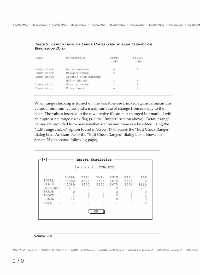
WeatherMan ¥ WeatherMan ¥ WeatherMan ¥ WeatherMan ¥ WeatherMan ¥ WeatherMan ¥ WeatherMan ¥ WeatherMan ¥ WeatherMan ¥ WeatherMa
DSSAT v3, Volume 3 ¥ DSSAT v3, Volume 3 ¥ DSSAT v3, Volume 3 ¥ DSSAT v3, Volume 3 ¥ DSSAT v3, Volume 3 ¥ DSSAT v3, Volume 3 ¥ DSSAT v3, V
170
When range checking is turned on, the variables are checked against a maximumvalue, a minimum value, and a maximum rate of change from one day to thenext. The values inserted in the raw archive file are not changed but marked withan appropriate range check flag (see the ÒImportÓ section above). Default rangevalues are provided for a new weather station and these can be edited using theÒEdit range checksÓ option found in Screen 17 to access the ÒEdit Check RangesÓdialog box. An example of the ÒEdit Check RangesÓ dialog box is shown inScreen 25 (on second following page).
Import Statistics[ ]
Records in UFGA.WTD
TOTAL :VALID :MISSING:ERROR :ABOVE :BELOW :RATE :
TOTAL433804308927701121
SRAD86768670
00060
TMAX86768673
00030
TMIN86768675
00001
RAIN86768676
00000
PAR867683952770130
OK
SCREEN 23.
TABLE 5. EXPLANATION OF ERROR CODES USED TO FLAG SUSPECT ORERRONEOUS DATA.
Class Description Import Filledcode code
Range check Above maximum a ARange check Below minimum b BRange check Greater than maximum
daily change r RConversion Missing value n NConversion Format error e E

WeatherMan ¥ WeatherMan ¥ WeatherMan ¥ WeatherMan ¥ WeatherMan ¥ WeatherMan ¥ WeatherMan ¥ WeatherMan ¥ WeatherMan ¥ WeatherMan ¥
¥ DSSAT v3, Volume 3 ¥ DSSAT v3, Volume 3 ¥ DSSAT v3, Volume 3 ¥ DSSAT v3, Volume 3 ¥ DSSAT v3, Volume 3 ¥ DSSAT v3, Volume 3 ¥ DSSAT v3, Volume
171
TABLE 6. EXPLANATION OF IMPORT OPTIONS.
Option Explanation
Format name: The default action is to prompt for a format name.If the only file formats used are the DSSAT v2.1 orDSSAT v3 formats, the format name can be fixed asIBSNAT v2 or IBSNAT v3, respectively.
Check ranges: The default is to perform range checking. The vari-ables are checked for extreme values and the unal-tered values are inserted in the raw data archivefile and marked with a flag (see Edit Range Checksbelow). Import operations can speeded up withoutrange checking and it can be performed later on thewhole archive file using an option in the Analyzemenu.
Overwrite existing data: If this option is enabled, when the existing and newdata both have valid values for the same dates, thenew values will replace the existing values. Turningoff this option causes the existing value to beretained under the same circumstances.
Prompt for non-numerics: The default action is to prompt the user to give anumeric value to replace each new non-numeric stringencountered (e.g., “TRACE” can be replaced with ‘0.0’for rainfall.) Turning off this option causes blanksto be treated as missing values and non-numeric char-acters to be treated as format errors.
Preview formats: The default action is to present a “Preview Format”dialog box (Screen 20) every time a file is importedor a format is edited during Import. Turning-offthis option prevents the “Preview Format” dialog boxfrom being displayed.

WeatherMan ¥ WeatherMan ¥ WeatherMan ¥ WeatherMan ¥ WeatherMan ¥ WeatherMan ¥ WeatherMan ¥ WeatherMan ¥ WeatherMan ¥ WeatherMa
172
SCREEN 24.
All variables in Screen 25 are in the archive file units except for solar radiation(SRAD) and photosynthetically active radiation (PAR) which are in percent ofextraterrestrial radiation. Updated ranges are saved to the weather station cli-mate file. The DEFAULTS button restores the default values.
[ ] Edit Check Ranges
Variable SRAD* TMAX TMIN RAIN DEWP WIND SUNH PAR * TDRY TWET EVAP
Minimum Maximum MaxRate5.05.0
-20.00.00.00.00.05.00.00.00.0
85.040.030.0600.025.0500.0100.085.035.025.015.0
70.020.020.0500.05.0
300.090.070.020.020.015.0
*Radiation in % of extraterrestrial.
OK Defaults Cancel
SCREEN 25.
Import Options
Format name: ( ) Prompt for name. ( ) IBSNAT3 ( ) IBSNAT2
Other options: [X] Check ranges. [X] Overwrite existing data. [X] Prompt for non-numerics. [X] Preview formats
CancelOK
[ ]

WeatherMan ¥ WeatherMan ¥ WeatherMan ¥ WeatherMan ¥ WeatherMan ¥ WeatherMan ¥ WeatherMan ¥ WeatherMan ¥ WeatherMan ¥ WeatherMan ¥
¥ DSSAT v3, Volume 3 ¥ DSSAT v3, Volume 3 ¥ DSSAT v3, Volume 3 ¥ DSSAT v3, Volume 3 ¥ DSSAT v3, Volume 3 ¥ DSSAT v3, Volume 3 ¥ DSSAT v3, Volume
173
EXPORT...The ÒExport...Ó option in Screen 17 can be used to export a single file or a set ofyearly files. The ÒExport single fileÓ option uses the ÒArchive TypeÓ dialog box(Screen 4) (if the raw archive file is not the only type), ÒTime PeriodÓ dialog box(Screen 5), and the ÒFile ListÓ dialog box (Screen 2) to select an export file nameand format. The ÒExport yearly fileÓ option uses the same dialog boxes, but thefile export names are built automatically based on the DSSAT v2.1 or DSSAT v3file naming conventions. The files can easily be renamed using the DOSRENAME command. Access to the ÒEdit FormatÓ dialog box is from theÒFormat FileÓ dialog box.
During ÒImport,Ó errors or suspect values in the raw archive file are markedwith a flag indicating the source of the error. On ÒExport,Ó if a data item is filledin, the valueÕs error flag is converted to an upper case letter. This reminds theuser that the value was filled-in and the cause of the error. Error flag definitionsare listed in Table 5.
EXPORT OPTIONS
The options for export can be changed using theÓExport optionsÓ menu itemwhich accesses the ÒExport OptionsÓ dialog box presented in Screen 26 (on fol-lowing page) and discussed in Table 7.
When any of the data fill options are turned on in Screen 26 by placing an ÔxÕ inthe left-hand box in the ÒOther options:Ó menu list, there are a number of waysin which the data fill can be implemented. These options are accessed from theÒData fillÓ options menu item that invokes theÓ Data Fill OptionsÓ dialog boxgiven in Screen 27 (on following page) and discussed in Table 8.
GE N E R AT E ME N U
The GENERATE menu item found on the WeatherMan main menu allows esti-mation of the weather generator parameters and subsequent generation of dailyweather data. The weather generators used are adaptations of WGEN(Richardson and Wright, 1984) and SIMMETEO (Geng et al. 1986; Geng andAuburn, 1988). The SIMMETEO generator is embodied in the WGEN generatorbut uses a different input section. The resulting WGEN/SIMMETEO is a transla-tion of the FORTRAN version used internally in the DSSAT v3 crop models. Inthis version of WeatherMan, both generators are restricted to generating theDSSAT v2.1 extended weather data set of solar radiation, maximum temperature,minimum temperature, rainfall, and PAR.

WeatherMan ¥ WeatherMan ¥ WeatherMan ¥ WeatherMan ¥ WeatherMan ¥ WeatherMan ¥ WeatherMan ¥ WeatherMan ¥ WeatherMan ¥ WeatherMa
DSSAT v3, Volume 3 ¥ DSSAT v3, Volume 3 ¥ DSSAT v3, Volume 3 ¥ DSSAT v3, Volume 3 ¥ DSSAT v3, Volume 3 ¥ DSSAT v3, Volume 3 ¥ DSSAT v3, V
174
F1 Help Stn: UFGA | Prompt for a format name on export.
[ ] Export Options
Format name: ( ) Prompt for name. ( ) IBSNAT3 ( ) IBSNAT2
Yearly filenaming conventions: ( ) IBSNAT v.3 ( ) IBSNAT v.2
Other options: [X] Fill missing data. [X] Fill range errors. [ ] Fill missing dates. [ ] Export data flags.
OK Cancel
SCREEN 26.
File Station Import/Export Generate Analyze Options Quit 14:19:23
F1 Help Stn: UFGA | Use a stochastic generator to fill missing data.
OK Cancel
[ ] Data Fill Options
Data fill method: ( ) Generate missing data with WGEN or SIMMETEO. ( ) Monthly means and stochastic rainfall generations.
Solar radiation (SRAD and PAR): ( ) Use method selected above to estimate radiation. ( ) Estimate radiation from sunshine hours.
Short (≤ 7 day) data gaps: ( ) Use method selected above to fill data. ( ) Estimate missing data using 10-day running mean.
Random seed for generator (1 to 32767): 3823
Model for weather generation: ( ) WGEN ( ) SIMMETEO
SCREEN 27.

WeatherMan ¥ WeatherMan ¥ WeatherMan ¥ WeatherMan ¥ WeatherMan ¥ WeatherMan ¥ WeatherMan ¥ WeatherMan ¥ WeatherMan ¥ WeatherMan ¥
¥ DSSAT v3, Volume 3 ¥ DSSAT v3, Volume 3 ¥ DSSAT v3, Volume 3 ¥ DSSAT v3, Volume 3 ¥ DSSAT v3, Volume 3 ¥ DSSAT v3, Volume 3 ¥ DSSAT v3, Volume
175
TABLE 7. EXPLANATION OF EXPORT OPTIONS.
Option Explanation
Format name: The default action is to prompt for a formatname. If the only file formats used are theDSSAT v2.1 or DSSAT v3 formats, the formatname can be fixed as IBSNAT v2 or IBSNAT v3,respectively.
Yearly file naming convention: The default is to use the DSSAT v3 file nam-ing convention. The other option is to usethe DSSAT v2 convention. The file namingconventions are (Station = 4 characters, yr =2 characters):
For DSSAT v2.1, useIBSNAT v2: Station + ‘0112.W’ + yr (raw)
Station + ‘GEN.W’ + yr (generated)
For DSSAT v3, useIBSNAT v3: Station + yr + ‘01.WTH’(raw)
Station + yr + ‘01.WTG’ (generat-ed)
Fill missing data: The default is to fill missing data. Ifmissing data are not filled, the value iswritten as -99.0 on output.
Fill range errors: The default is to replace data that areflagged for range errors. This option isonly in effect if Fill Missing Data ischecked. If range errors are not filled, theoriginal value is written on output.
Fill missing dates: The default is to fill missing dates withsequential dates and fill variable values.If Fill Missing Dates is disabled, missingdates in the raw archive file will also existin the output file.
Export Data Flags: The default is to export the error flags aslower case if data are not filled and uppercase if they were filled. If data are filledand error flags are not exported, there willbe no indication that the data have been
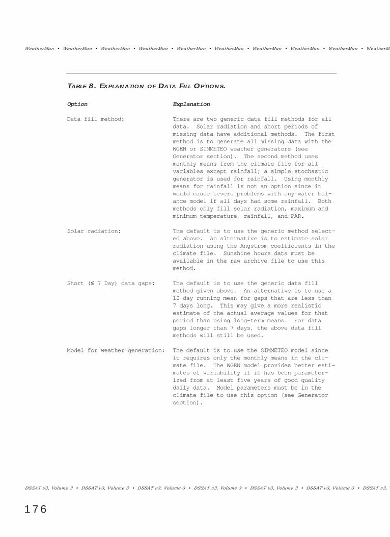
WeatherMan ¥ WeatherMan ¥ WeatherMan ¥ WeatherMan ¥ WeatherMan ¥ WeatherMan ¥ WeatherMan ¥ WeatherMan ¥ WeatherMan ¥ WeatherMa
DSSAT v3, Volume 3 ¥ DSSAT v3, Volume 3 ¥ DSSAT v3, Volume 3 ¥ DSSAT v3, Volume 3 ¥ DSSAT v3, Volume 3 ¥ DSSAT v3, Volume 3 ¥ DSSAT v3, V
176
TABLE 8. EXPLANATION OF DATA FILL OPTIONS.
Option Explanation
Data fill method: There are two generic data fill methods for alldata. Solar radiation and short periods ofmissing data have additional methods. The firstmethod is to generate all missing data with theWGEN or SIMMETEO weather generators (seeGenerator section). The second method usesmonthly means from the climate file for allvariables except rainfall; a simple stochasticgenerator is used for rainfall. Using monthlymeans for rainfall is not an option since itwould cause severe problems with any water bal-ance model if all days had some rainfall. Bothmethods only fill solar radiation, maximum andminimum temperature, rainfall, and PAR.
Solar radiation: The default is to use the generic method select-ed above. An alternative is to estimate solarradiation using the Angstrom coefficients in theclimate file. Sunshine hours data must beavailable in the raw archive file to use thismethod.
Short (≤ 7 Day) data gaps: The default is to use the generic data fillmethod given above. An alternative is to use a10-day running mean for gaps that are less than7 days long. This may give a more realisticestimate of the actual average values for thatperiod than using long-term means. For datagaps longer than 7 days, the above data fillmethods will still be used.
Model for weather generation: The default is to use the SIMMETEO model sinceit requires only the monthly means in the cli-mate file. The WGEN model provides better esti-mates of variability if it has been parameter-ized from at least five years of good qualitydaily data. Model parameters must be in theclimate file to use this option (see Generatorsection).

WeatherMan ¥ WeatherMan ¥ WeatherMan ¥ WeatherMan ¥ WeatherMan ¥ WeatherMan ¥ WeatherMan ¥ WeatherMan ¥ WeatherMan ¥ WeatherMan ¥
¥ DSSAT v3, Volume 3 ¥ DSSAT v3, Volume 3 ¥ DSSAT v3, Volume 3 ¥ DSSAT v3, Volume 3 ¥ DSSAT v3, Volume 3 ¥ DSSAT v3, Volume 3 ¥ DSSAT v3, Volume
177
The DSSAT v3 modifications of WGEN/SIMMETEO use standard deviationsrather than coefficients of variation which makes the generators more stable thanthe original versions. Monthly input parameters are now used for all variables,with linear interpolation computed internally. The modified SIMMETEO modeluses monthly climate parameters and regression equations (Geng, et al. 1988;Geng and Auburn, 1986; Pickering et al. 1988) to compute the standard devia-tions.
The GENERATE menu provides the utilities necessary for estimating the genera-tor parameters and generating daily data. The GENERATE menu is shown inScreen 28 (below) and its options are described as follows.
CALCULATE PARAMETERS
When the ÒCalculate parametersÓ option shown in Screen 28 is selected, theÒCalculate ParametersÓ dialog box, shown in Screen 29 (on following page), ispresented.
From Screen 29, the parameters for WGEN or SIMMETEO can be computed sepa-rately or together. A standard ÒTime PeriodÓ dialog box (i.e., ÒStartingÓ andÒEndingÓ dates) is included in the dialog box shown in Screen 29, allowing you tochoose a particular time period if desired. The default is to use all the data in thearchive file, and the dates presented when Screen 29 appears should represent therange of dates available in the archive file. The computed monthly parametersare recorded in the climate file. Estimating the SIMMETEO parameters is equiva-lent to calculating monthly means from the STATION menu (see Screen 14)Ñboth
File Station Import/Export Generate Analyze Options Quit 14:55:44
Calculate parameters
Generate data
SCREEN 28.

Calculate Parameters
Starting date:
Ending date:
Year yearDay of
OK
1
3651987
1980
Model: ( ) WGEN generator parameter ( ) SIMMETEO monthly means ( ) Both sets of parameters
[ ]
Cancel
WeatherMan ¥ WeatherMan ¥ WeatherMan ¥ WeatherMan ¥ WeatherMan ¥ WeatherMan ¥ WeatherMan ¥ WeatherMan ¥ WeatherMan ¥ WeatherMa
DSSAT v3, Volume 3 ¥ DSSAT v3, Volume 3 ¥ DSSAT v3, Volume 3 ¥ DSSAT v3, Volume 3 ¥ DSSAT v3, Volume 3 ¥ DSSAT v3, Volume 3 ¥ DSSAT v3, V
178
calculate the same statistics. If the monthly means in the climate file are from alonger and more reliable record than the daily data, the user should not estimateSIMMETEOÕs parameters since the monthly means in the climate file will be over-written. Estimating generator parameters is a reasonable option if there are suffi-cient reliable data in the raw archive file or if there are no available climate data.The user is warned if there are less than five years of reliable data in the archive file.
GENERATE DATA
The ÒGenerate dataÓ menu item accesses the ÒGenerate Weather DataÓ dialog boxwhich is shown in Screen 30 (on following page).
Generated data are output to an archive file called Station_GEN.WTD. This file isusually treated as a temporary file for the duration of the WeatherMan session (seethe following section entitled, ÒOptions MenuÓ and the subsection ÒTemporaryFilesÓ for a description of how to change from a temporary file). Either the WGENor SIMMETEO generator can be used to generate daily data. The standard ÒTimePeriodÓ dialog box is inserted to choose the years to be generated; only full years canbe generated. The default action is to match the time period of the raw archive file,although any time period can be specified. For comparing yearly time series graphi-cally, matching the dates is a good choice. Just because generated and raw data havethe same time period does not mean that the generated data predict the raw dailydata; only the means are predicted on average. A random number seed is generatedand inserted in the dialog box shown in Screen 30. To generate an identical sequenceof weather data, the same random number seed should be specified.
SCREEN 29.

WeatherMan ¥ WeatherMan ¥ WeatherMan ¥ WeatherMan ¥ WeatherMan ¥ WeatherMan ¥ WeatherMan ¥ WeatherMan ¥ WeatherMan ¥ WeatherMan ¥
¥ DSSAT v3, Volume 3 ¥ DSSAT v3, Volume 3 ¥ DSSAT v3, Volume 3 ¥ DSSAT v3, Volume 3 ¥ DSSAT v3, Volume 3 ¥ DSSAT v3, Volume 3 ¥ DSSAT v3, Volume
179
The ANALYZE menu item found on the WeatherMan main menu allows you tocalculate and present summary statistics in both tabular and graphical form. Italso repeats the range check and data fill functions that are normally done auto-matically on IMPORT or EXPORT. Analysis is performed on raw, filled or gener-ated data. The ANALYZE menu is shown in Screen 31 (on following page) andits options described as follows.
RANGE CHECK AND DATA FILL
The ÒRange checkÓ and ÒData fillÓ options listed in Screen 31 offer you anotherway to perform functions normally done on IMPORT or EXPORT.
Range check. The ÒRange checkÓ option permits the range checking analysisto be done on the complete raw archive file. After the check is done, the resultsare given in an ÒImport StatisticsÓ dialog box similar to the dialog box forIMPORT (see Screen 23). This re-checking process is useful when IMPORT hasbeen done with incorrect range check values or if range checking had beenturned off during IMPORT. It is also useful for identifying a reasonable set ofrange check values for a weather station by iteratively setting the range checkvalues and viewing the results.
Generate Weather Data[ ]
Model: ( ) WGEN ( ) SIMMETEO
Starting year:
Ending year:
1980
1987
Random seed (1 to 32767):3919
OK Cancel
SCREEN 30.
AN A LY Z E ME N U

WeatherMan ¥ WeatherMan ¥ WeatherMan ¥ WeatherMan ¥ WeatherMan ¥ WeatherMan ¥ WeatherMan ¥ WeatherMan ¥ WeatherMan ¥ WeatherMa
DSSAT v3, Volume 3 ¥ DSSAT v3, Volume 3 ¥ DSSAT v3, Volume 3 ¥ DSSAT v3, Volume 3 ¥ DSSAT v3, Volume 3 ¥ DSSAT v3, Volume 3 ¥ DSSAT v3, V
180
Data fill. The ÒData fillÓ option creates a filled archive file calledStation_FIL.WTD. This file is usually treated as a temporary file for the durationof the WeatherMan session (see the following section entitled, ÒOptions MenuÓand the subsection ÒTemporary FilesÓ for a description of how to change from atemporary file). The filled archive file can be analyzed and compared with theraw data to check the data fill algorithms.
STATISTICS
The ÒStatisticsÓ menu item listed in Screen 31 provides algorithms for summariz-ing the data in various ways. When this option is selected, the ÒArchive TypeÓdialog box is presented (Screen 32, on following page). This dialog box allowsyou to choose raw, filled, or generated archive files.
Statistics are output to summary files and are usually treated as temporary filesfor the duration of the WeatherMan session ( see the following section entitled,ÒOptions MenuÓ and the subsection ÒTemporary FilesÓ for a description of howto change from a temporary file). The SUM files are also used for the ÒReportÓand ÒGraphÓ options under the ANALYZE menu. The ÒTime PeriodÓ dialog boxallows the user to choose the time period to be analyzed. The default action is toanalyze the whole archive file.
In Screen 32, there are four types of statistics to select from: ÒMoments,ÓÒPercentiles,Ó ÒDistributionÓ and ÒTime structure.Ó The default choice is to cal-culate moments only. ÒMomentsÓ includes means, standard deviations, and
File Station Import/Export Generate Analyze Options Quit 14:55:44
Range checkData fill
StatisticsReport
Graph
SCREEN 31.
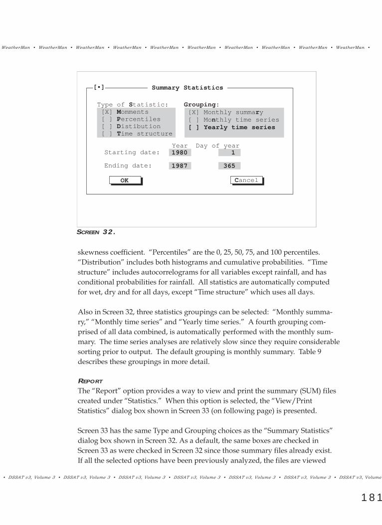
WeatherMan ¥ WeatherMan ¥ WeatherMan ¥ WeatherMan ¥ WeatherMan ¥ WeatherMan ¥ WeatherMan ¥ WeatherMan ¥ WeatherMan ¥ WeatherMan ¥
¥ DSSAT v3, Volume 3 ¥ DSSAT v3, Volume 3 ¥ DSSAT v3, Volume 3 ¥ DSSAT v3, Volume 3 ¥ DSSAT v3, Volume 3 ¥ DSSAT v3, Volume 3 ¥ DSSAT v3, Volume
181
skewness coefficient. ÒPercentilesÓ are the 0, 25, 50, 75, and 100 percentiles.ÒDistributionÓ includes both histograms and cumulative probabilities. ÒTimestructureÓ includes autocorrelograms for all variables except rainfall, and hasconditional probabilities for rainfall. All statistics are automatically computedfor wet, dry and for all days, except ÒTime structureÓ which uses all days.
Also in Screen 32, three statistics groupings can be selected: ÒMonthly summa-ry,Ó ÒMonthly time seriesÓ and ÒYearly time series.Ó A fourth grouping com-prised of all data combined, is automatically performed with the monthly sum-mary. The time series analyses are relatively slow since they require considerablesorting prior to output. The default grouping is monthly summary. Table 9describes these groupings in more detail.
REPORT
The ÒReportÓ option provides a way to view and print the summary (SUM) filescreated under ÒStatistics.Ó When this option is selected, the ÒView/PrintStatisticsÓ dialog box shown in Screen 33 (on following page) is presented.
Screen 33 has the same Type and Grouping choices as the ÒSummary StatisticsÓdialog box shown in Screen 32. As a default, the same boxes are checked inScreen 33 as were checked in Screen 32 since those summary files already exist.If all the selected options have been previously analyzed, the files are viewed
[ ] Summary Statistics
Type of Statistic: [X] Momments [ ] Percentiles [ ] Distibution [ ] Time structure
Grouping: [X] Monthly summary [ ] Monthly time series [ ] Yearly time series
Year Day of year
OK Cancel
Starting date:
Ending date:
1980
1987
1
365
SCREEN 32.

WeatherMan ¥ WeatherMan ¥ WeatherMan ¥ WeatherMan ¥ WeatherMan ¥ WeatherMan ¥ WeatherMan ¥ WeatherMan ¥ WeatherMan ¥ WeatherMa
DSSAT v3, Volume 3 ¥ DSSAT v3, Volume 3 ¥ DSSAT v3, Volume 3 ¥ DSSAT v3, Volume 3 ¥ DSSAT v3, Volume 3 ¥ DSSAT v3, Volume 3 ¥ DSSAT v3, V
182
[ ] View/Print Statistics
Type of Statistic: [X] Momments [ ] Percentiles [ ] Distibution [ ] Time structure
Grouping: [X] Monthly summary [ ] Monthly time series [ ] Yearly time series
OK Cancel
SCREEN 33.
sequentially. Up to 12 summary files are possible for each type of archive file.When the OK button is pressed in Screen 33, the ÒSummary FileÓ dialog boxshown in Screen 34 (on following page) is presented.
The user can scroll both vertically and horizontally through the SUM file dis-played in Screen 34. If the PRINT button in Screen 34 is pressed, the SUM filedisplayed in the window is printed to the parallel printer port. The OK buttondisplays the next file while the CANCEL button aborts the viewing process.
TABLE 9. EXPLANATION OF STATISTICS TIME GROUPINGS.
Grouping Explanation
All data combined Pools all data together (computed automatically withmonthly summary).
Monthly summary Pools all the data from each month together (eg. all ofJanuary’s, all of February’s etc).
Monthly time series Each month analyzed separately.
Yearly time series Each year analyzed separately.

WeatherMan ¥ WeatherMan ¥ WeatherMan ¥ WeatherMan ¥ WeatherMan ¥ WeatherMan ¥ WeatherMan ¥ WeatherMan ¥ WeatherMan ¥ WeatherMan ¥
¥ DSSAT v3, Volume 3 ¥ DSSAT v3, Volume 3 ¥ DSSAT v3, Volume 3 ¥ DSSAT v3, Volume 3 ¥ DSSAT v3, Volume 3 ¥ DSSAT v3, Volume 3 ¥ DSSAT v3, Volume
183
Variable names that appear in summary files are given in Appendix A.
GRAPH
The ÒGraphÓ option provides access to a graphics package to plot both the datain the archive files and in the statistics (SUM) files. The following six graph typesare available: Time Plot, Box Plot, Histogram, Cumulative Distribution,Autocorrelation, and Rainfall Probability. Within each graph type, up to six plotscan be defined (except for the Box Plot and Auto correlation which allow only asingle plot), but only the checked plots will actually be plotted. A plot definitiondialog box is used to create combinations of weather stations, variables, wetstates, and time ranges. A default set of plots is automatically loaded into thisdialog box. The down arrow or mouse can be used to access lists for the Station,Variable and Wet state columns. Only valid choices are displayed. For example,if statistics have not been calculated for a particular weather station, the statisticsvariables for that station will not be displayed. In addition, the Wet state columnis not visible for a daily time grouping. The wet state refers to the occurrence ofrainfall; choices are Wet, Dry, or All.
An example of a plot definition dialog box is given in Screen 35 (on followingpage) for a ÒTime Plot RangeÓ where six plots are defined and two (TMAX andTMIN) are checked for plotting.
[ ] Summary FileUFGA_AMA.SUM
File Station Import/Export Generate Analyze Options Quit
OK Cancel
! Monthly summary moments for station UFGA observed data.
*SRADDRY
@ MTH SDMN SDSD SDSK SDKT 1 11.9 2.9 -0.9 0.3 2 14.8 3.7 -0.9 0.3 3 18.8 4.1 -0.8 0.0 4 22.7 3.8 -1.1 1.6 5 23.4 3.8 -1.1 1.2 6 22.4 3.6 -0.8 0.3 7 22.0 3.4 -0.9 1.0 8 20.3 2.9 -0.8 0.6 9 17.7 3.3 -1.0 0.8 10 15.4 3.4 -0.9 0.7
F1 Help Stn: UFGA | Use cursor keys or mouse to scroll, <Esc> or icon to quit.
SCREEN 34.

WeatherMan ¥ WeatherMan ¥ WeatherMan ¥ WeatherMan ¥ WeatherMan ¥ WeatherMan ¥ WeatherMan ¥ WeatherMan ¥ WeatherMan ¥ WeatherMa
DSSAT v3, Volume 3 ¥ DSSAT v3, Volume 3 ¥ DSSAT v3, Volume 3 ¥ DSSAT v3, Volume 3 ¥ DSSAT v3, Volume 3 ¥ DSSAT v3, Volume 3 ¥ DSSAT v3, V
184
The TYPE , GROUPING and RANGE buttons in Screen 35 control the graphchoices, while the GRAPH button displays the graph, and the CANCEL buttonexits the dialog box. The TYPE button provides a choice of six graph types in theÒGraph TypeÓ dialog box that overlays the plot definition dialog box as shown inScreen 36 (below).
The GROUPING button accesses a ÒSelect GroupingÓ dialog box similar to theright hand side of the ÒSummary StatisticsÓ (Screen 32) or ÒView/Print StatisticsÓ
[ ] Time Plot Range
PlotNum. Station Variable
Type
Grouping
Range
Graph
Cancel
123456
[X][ ][ ][ ][ ][ ]
UFGA RAWUFGA RAWUFGA RAWUFGA RAWUFGA RAWUFGA RAW
SPRADTMAXTMINRAINPAR
↓↓↓↓↓↓
↓↓↓↓↓↓
SCREEN 35.
[ ] Time Plot Range
PlotNum. Station Variable
Type
Grouping
Range
Graph
Cancel
123456
[X][ ][ ][ ][ ][ ]
UFGA RAWUFGA RAWUFGA RAWUFGA RAWUFGA RAWUFGA RAW
SPRADTMAXTMINRAINPAR
↓↓↓↓↓↓
↓↓↓↓↓↓
Graph Type[ ]
Type of Graph: ( ) Time plot ( ) Box plot ( ) Histogram ( ) Cumul. distribution ( ) Autocorrelation ( ) Rainfall probability
OK Cancel
SCREEN 36.
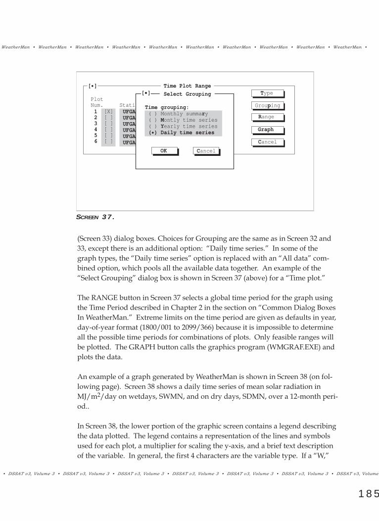
WeatherMan ¥ WeatherMan ¥ WeatherMan ¥ WeatherMan ¥ WeatherMan ¥ WeatherMan ¥ WeatherMan ¥ WeatherMan ¥ WeatherMan ¥ WeatherMan ¥
¥ DSSAT v3, Volume 3 ¥ DSSAT v3, Volume 3 ¥ DSSAT v3, Volume 3 ¥ DSSAT v3, Volume 3 ¥ DSSAT v3, Volume 3 ¥ DSSAT v3, Volume 3 ¥ DSSAT v3, Volume
185
(Screen 33) dialog boxes. Choices for Grouping are the same as in Screen 32 and33, except there is an additional option: ÒDaily time series.Ó In some of thegraph types, the ÒDaily time seriesÓ option is replaced with an ÒAll dataÓ com-bined option, which pools all the available data together. An example of theÒSelect GroupingÓ dialog box is shown in Screen 37 (above) for a ÒTime plot.Ó
The RANGE button in Screen 37 selects a global time period for the graph usingthe Time Period described in Chapter 2 in the section on ÒCommon Dialog BoxesIn WeatherMan.Ó Extreme limits on the time period are given as defaults in year,day-of-year format (1800/001 to 2099/366) because it is impossible to determineall the possible time periods for combinations of plots. Only feasible ranges willbe plotted. The GRAPH button calls the graphics program (WMGRAF.EXE) andplots the data.
An example of a graph generated by WeatherMan is shown in Screen 38 (on fol-lowing page). Screen 38 shows a daily time series of mean solar radiation inMJ/m2/day on wetdays, SWMN, and on dry days, SDMN, over a 12-month peri-od..
In Screen 38, the lower portion of the graphic screen contains a legend describingthe data plotted. The legend contains a representation of the lines and symbolsused for each plot, a multiplier for scaling the y-axis, and a brief text descriptionof the variable. In general, the first 4 characters are the variable type. If a ÒW,Ó
[ ] Time Plot Range
PlotNum. Station Variable
Type
Grouping
Range
Graph
Cancel
123456
[X][ ][ ][ ][ ][ ]
UFGA RAWUFGA RAWUFGA RAWUFGA RAWUFGA RAWUFGA RAW
SPRADTMAXTMINRAINPAR
↓↓↓↓↓↓
↓↓↓↓↓↓
[ ] Select Grouping
Time grouping: ( ) Monthly summary ( ) Montly time series ( ) Yearly time series ( ) Daily time series
OK Cancel
SCREEN 37.

WeatherMan ¥ WeatherMan ¥ WeatherMan ¥ WeatherMan ¥ WeatherMan ¥ WeatherMan ¥ WeatherMan ¥ WeatherMan ¥ WeatherMan ¥ WeatherMa
DSSAT v3, Volume 3 ¥ DSSAT v3, Volume 3 ¥ DSSAT v3, Volume 3 ¥ DSSAT v3, Volume 3 ¥ DSSAT v3, Volume 3 ¥ DSSAT v3, Volume 3 ¥ DSSAT v3, V
186
25.00
20.00
15.00
10.00
0.00 4.00 8.00 12.00 16.00
(1) SWMN(W),UFGARAW,ALL
Time Plot
(1) SDMN(D),UFGARAW,ALL
SCREEN 38.
ÒD,Ó or ÒAÓ appears in parentheses, it represents wet state (i.e., wet, dry, or all).The next four characters following the first comma are the station name, followedby ÒRAWÓ (observed data), ÒGENÓ (generated data), or ÒFILÓ (observed datawith any missing or suspect data filled-in). The text following the final commarepresents the time period (month, year, or ÒALLÓ). Variable names that appearin graphs are defined in Appendix A.
OP T I O N S ME N U
The OPTIONS menu item found on the WeatherMan main menu allows you tochange and save options and defaults. The OPTIONS menu is shown in Screen39 (on following page) and its options are described as follows.
NOTE: Unless the ÒUpdate optionsÓ option is selected first, the menu options listed inScreen 38 are only for the WeatherMan session you are currently working in.

WeatherMan ¥ WeatherMan ¥ WeatherMan ¥ WeatherMan ¥ WeatherMan ¥ WeatherMan ¥ WeatherMan ¥ WeatherMan ¥ WeatherMan ¥ WeatherMan ¥
¥ DSSAT v3, Volume 3 ¥ DSSAT v3, Volume 3 ¥ DSSAT v3, Volume 3 ¥ DSSAT v3, Volume 3 ¥ DSSAT v3, Volume 3 ¥ DSSAT v3, Volume 3 ¥ DSSAT v3, Volume
187
DISPLAY MODE
When the ÒDisplay modeÓ option is selected, the ÒVideo ModeÓ dialog boxshown in Screen 40 (below) is presented.
The ÒVideo modeÓ window in Screen 40 is best left on ÒAutodetectÓ unless theprogram has difficulty selecting the correct mode and a manual choice of an alter-
File Station Import/Export Generate Analyze Options Quit 14:50:09
Display modeColors
DirectoriesTemporary files
Graph colorsGraph output
Update options
SCREEN 39.
Video Mode
Video mode: ( ) Autodetect mode ( ) Color palette ( ) Black & White palette ( ) Monochrome palette ( ) Custom palette
OK Cancel
[ ]
SCREEN 40.

WeatherMan ¥ WeatherMan ¥ WeatherMan ¥ WeatherMan ¥ WeatherMan ¥ WeatherMan ¥ WeatherMan ¥ WeatherMan ¥ WeatherMan ¥ WeatherMa
DSSAT v3, Volume 3 ¥ DSSAT v3, Volume 3 ¥ DSSAT v3, Volume 3 ¥ DSSAT v3, Volume 3 ¥ DSSAT v3, Volume 3 ¥ DSSAT v3, Volume 3 ¥ DSSAT v3, V
188
native mode or color palette gives a better screen appearance. The LCD andplasma screens used on some portable computers often look better using aÒBlack and White paletteÓ than with the automatically detected color mode. Inaddition, the ÒColorsÓ option in Screen 39 allows you to create a custom colorpalette. You may change the WeatherMan program default colors by doing thefollowing: 1) select the ÒColorsÓ option, and choose your custom colors (seeScreen 41, above, and the section ÒColorsÓ below); 2) select the ÒDisplay modeÓoption (Screen 39) and select ÒCustom paletteÓ in Screen 40; 3) press the OK but-ton; and 4) select the ÒUpdateÓ menu option from the OPTIONS menu. Fromthat point on, whenever WeatherMan is started, your customized colors will beactive.
COLORS
The ÒColorsÓoption gives you access to the ÒColorsÓ dialog box which permitsthe default colors for the desktop (background), menus and dialog boxes to bechanged. In order for these colors to remain in effect in subsequent WeatherMansessions, following the description on how to do this in the above section,ÒDisplay mode.Ó The ÒColorsÓ dialog box is shown in Screen 41 (above).
Colors[ ]
Group Desktop Menus Dialogs
Item Color
Foreground
Background
Text Text TextText Text Text
OK CancelNOTE: Must select Custompalette to retain colors.
SCREEN 41.

WeatherMan ¥ WeatherMan ¥ WeatherMan ¥ WeatherMan ¥ WeatherMan ¥ WeatherMan ¥ WeatherMan ¥ WeatherMan ¥ WeatherMan ¥ WeatherMan ¥
¥ DSSAT v3, Volume 3 ¥ DSSAT v3, Volume 3 ¥ DSSAT v3, Volume 3 ¥ DSSAT v3, Volume 3 ¥ DSSAT v3, Volume 3 ¥ DSSAT v3, Volume 3 ¥ DSSAT v3, Volume
189
DIRECTORIES
When the ÒDirectoriesÓ option in Screen 39 is selected, the ÒDirectoriesÓ dialogbox, shown in Screen 42 (above), is presented. This dialog box permits you tochange the default directories and editor.
All the information listed in Screen 42 can also be obtained from the DSSAT v3profile file called DSSATPRO.FLE (see Volume 1-3, Hunt et al. 1994, of this bookfor a description of this file). When the ÒObtain directories fromDSSATPRO.FLEÓ box in Screen 42 is checked, directories that conflict with thosein DSSATPRO.FLE are disregarded. This box should generally be checked onlywhen running WeatherMan under DSSAT v3.
The directory, name, and any command line options for the userÕs favorite editorcan replace the default editor.
TEMPORARY FILES
When the ÒTemporary filesÓ option is selected, the ÒTemporary File OptionsÓ dia-log box, shown in Screen 43 (on following page), is presented. From this dialogbox, you can control the status of temporary files.
The files that are temporary are filled and generated archive (WTD) files and sta-
[ ] Directories
[X] Obtain directories from DSSATPRO.FLE.
Weather data:
Climate files:
Graphics program:
Graphic output:
Editor path & file:Editor command line
C:\DSSAT3\WEATHER\
C:\DSSAT3\WEATHER\CLIMATE\
C:\DSSAT3\
C:\DSSAT3\WEATHER\
C:DOS\EDIT.COM
OK Cancel
SCREEN 42.

WeatherMan ¥ WeatherMan ¥ WeatherMan ¥ WeatherMan ¥ WeatherMan ¥ WeatherMan ¥ WeatherMan ¥ WeatherMan ¥ WeatherMan ¥ WeatherMa
DSSAT v3, Volume 3 ¥ DSSAT v3, Volume 3 ¥ DSSAT v3, Volume 3 ¥ DSSAT v3, Volume 3 ¥ DSSAT v3, Volume 3 ¥ DSSAT v3, Volume 3 ¥ DSSAT v3, V
190
tistics (SUM) files. These files should normally be deleted to avoid wasting diskspace, but may be retained if desired. For example, generation and analysis of avery long weather record may justify keeping the generated and statistics files.
GRAPH COLORS AND GRAPH OPTIONS
Both ÒGraph colors,Ó and ÒGraph optionsÓ allows you to set graph options.
Graph colors. When the ÒGraph colorsÓ option is selected, a ÒGraph ColorsÓdialog box dialog, as shown in Screen 44 (on following page), is presented, whichallows you to set the colors of the background and graph (lines).
Graph output. When the ÒGraph outputÓ option is selected, theÓGraph OutputOptionsÓ dialog box, shown in Screen 45 (on following page) is presented. In thisdialog box, you can specify the device, port and orientation for hardcopy output.
In Screen 45, you can select an output device type/resolution/paper size combi-nation from the scrolling list. If a ÒfileÓ is selected as the output port (see theoptions under the ÒPortÓ window), the user is prompted for a file name using astandard ÒFile ListÓ dialog box prior to entering the graphics program from theANALYZE|ÓGraphÓ menu item.
[ ] Temporary File Options
Filled and generatedarchived files: ( ) Discard at end of session. ( ) Prompt for each file. ( ) Keep at end of session.
Summary statistics files: ( ) Discard at end of session. ( ) Prompt for each file. ( ) Keep at end of session.
OK Cancel
SCREEN 43.

WeatherMan ¥ WeatherMan ¥ WeatherMan ¥ WeatherMan ¥ WeatherMan ¥ WeatherMan ¥ WeatherMan ¥ WeatherMan ¥ WeatherMan ¥ WeatherMan ¥
¥ DSSAT v3, Volume 3 ¥ DSSAT v3, Volume 3 ¥ DSSAT v3, Volume 3 ¥ DSSAT v3, Volume 3 ¥ DSSAT v3, Volume 3 ¥ DSSAT v3, Volume 3 ¥ DSSAT v3, Volume
191
Graph Output Options[ ]
Output drivers Epson 9 Pin 60 x 72 dpi Epson 9 Pin 120 x 72 dpi Epson 9 Pin 240 x 216 dpi Epson 24 Pin 180 x 180 dpi Epson 24 Pin 360 x 180 dpi Epson 24 Pin 360 x 360 dpi HP LaserJet/DeskJet B&W 100 dpi HP LaserJet/DeskJet B&W 150 dpi HP LaserJet/DeskJet B&W 300 dpi HP DeskJet 500C 100 dpi 8 color
Port ( ) LPT1 ( ) LPT2 ( ) COM1 ( ) COM2 ( ) file
OK Cancel
Orientation: ( ) Portrait ( ) Landscape
SCREEN 45.
UPDATE OPTIONS
Selecting the ÒUpdate optionsÓ menu item allows you to save the options youhave selected. All WeatherMan options are saved to the configuration file
Graph Colors[ ]
Group Background Graph
Item Axes & Labels Plot range #1 Plot range #2 Plot range #3 Plot range #4 Plot range #5 Plot range #6
Color
OK Cancel
SCREEN 44.

WeatherMan ¥ WeatherMan ¥ WeatherMan ¥ WeatherMan ¥ WeatherMan ¥ WeatherMan ¥ WeatherMan ¥ WeatherMan ¥ WeatherMan ¥ WeatherMa
DSSAT v3, Volume 3 ¥ DSSAT v3, Volume 3 ¥ DSSAT v3, Volume 3 ¥ DSSAT v3, Volume 3 ¥ DSSAT v3, Volume 3 ¥ DSSAT v3, Volume 3 ¥ DSSAT v3, V
192
QU I T ME N U
WM.CFG while Graphics program options are saved to DEVICE.FLE and GCON-FIG.FLE. These options are then used the next time WeatherMan is started.
When the QUIT menu item is selected from the WeatherMan main menu, youcan choose to exit the program. You may also use the <ALT>-<Q> key sequenceas a shortcut key sequence to quit. The user may also use the shortcut-keyoptions, <ALT>-<X> or <ALT>-<FX>, under the FILE menu to quit theWeatherMan program.

WeatherMan ¥ WeatherMan ¥ WeatherMan ¥ WeatherMan ¥ WeatherMan ¥ WeatherMan ¥ WeatherMan ¥ WeatherMan ¥ WeatherMan ¥ WeatherMan ¥
¥ DSSAT v3, Volume 3 ¥ DSSAT v3, Volume 3 ¥ DSSAT v3, Volume 3 ¥ DSSAT v3, Volume 3 ¥ DSSAT v3, Volume 3 ¥ DSSAT v3, Volume 3 ¥ DSSAT v3, Volume
193
Borland. 1993. Borland Pascal Version 7. Borland International, Scotts Valley,California.
Conway, H.M. Jr, S.L. May Jr., and E. Armstrong, Jr. 1963. The Weather Handbook.Conway Publications, Atlanta, GA.
Geng, S., J.S. Auburn, E. Brandsetter and B. Li. 1988. A program to simulate metero-logical variables: Documentation for SIMMETEO. Agronomy Progress report No.204. Dept. of Agronomy and Range Sci., Univ. of California, Davis, CA.
Geng, S. and J.S. Auburn. 1986. Weather simulation models based on summaries oflong-term data. In Intl. Symp. on Impact of Weather Parameters on the Growthand Yield of Rice, April 7-10. International Rice Research Institute, Los Banos,Philippines.
Hunt, L.A., J.W. Jones, P.K. Thornton, G. Hoogenboom, D.T. Imamura, G.Y. Tsuji andU. Singh. 1994. Accessing data, models and application programs. In: Tsuji, G.Y.,G. Uehara and S. Balas (eds.). DSSAT v3. Vol. 1-3. University of Hawaii,Honolulu, HI.
Jones, J.W., L.A. Hunt, G. Hoogenboom, D.C. Godwin, U. Singh, G.Y. Tsuji, N.Pickering, P.K. Thornton, W.T. Bowen, K.J. Boote and J.T. Ritchie. 1994. Input andoutput files. In: Tsuji, G.Y., G. Uehara and S. Balas (eds). DSSAT v3. Vol. 2-1.University of Hawaii, Honolulu, HI.
NOAA. 1974. Climate of the States. Water Information Center, NationalOceanographic and Atmospheric Administration, United States Department ofCommerce, Asheville, NC.
Pickering, N.B., J.W. Hansen, J.W. Jones, H. Chan, and D. Godwin. 1994.WeatherMan: A utility for managing and generating daily weather data. Agron. J.86(2):332-337.
Pickering, N.B., J.R. Stedinger, and D.A. Haith. 1988. Weather input for nonpoint-source pollution models. J. Irrig. Drain. Eng. 114(4):674-690.
Prescott, J.A. 1940. Evaporation from a water surface in relation to solar radiation.Trans. R. Soc. S. Austr. 64: 114-118.
REFERENCES

WeatherMan ¥ WeatherMan ¥ WeatherMan ¥ WeatherMan ¥ WeatherMan ¥ WeatherMan ¥ WeatherMan ¥ WeatherMan ¥ WeatherMan ¥ WeatherMa
DSSAT v3, Volume 3 ¥ DSSAT v3, Volume 3 ¥ DSSAT v3, Volume 3 ¥ DSSAT v3, Volume 3 ¥ DSSAT v3, Volume 3 ¥ DSSAT v3, Volume 3 ¥ DSSAT v3, V
194
Richardson, C.W. and D.A. Wright. 1984. WGEN: a model for generating dailyweather variables. United States Department of Agriculture, AgriculturalResearch Service, ARS-8, Washington, DC.
Rietveld, M.R. 1978. A new method for estimating the regression coefficients inthe formula relating solar radiation to sunshine. Agricul. Meterol. 19:243-252.
Rudloff, W. 1981. World-Climate. Wissenschaftliche Verlagsgesellschaft, mbHStuttgart, Germany.

WeatherMan ¥ WeatherMan ¥ WeatherMan ¥ WeatherMan ¥ WeatherMan ¥ WeatherMan ¥ WeatherMan ¥ WeatherMan ¥ WeatherMan ¥ WeatherMan ¥
¥ DSSAT v3, Volume 3 ¥ DSSAT v3, Volume 3 ¥ DSSAT v3, Volume 3 ¥ DSSAT v3, Volume 3 ¥ DSSAT v3, Volume 3 ¥ DSSAT v3, Volume 3 ¥ DSSAT v3, Volume
195
SRAD Total daily solar radiation.TMAX Maximum daily air temperature.TMIN Minimum daily air temperature.RAIN Total daily precipitation.DEWP Dew point temperature or vapor pressure.WIND Total daily wind run.SUNH Total daily sunshine hours.PAR Total daily photosynthetic radiation.TWET Wet bulb air temperature at 9 a.m.EVAP Total daily pan evaporation.
APPENDIX A. ABBREVIATIONS USED IN WEATHERMAN
DA I LY WE AT H E R VA R I A B L E S
Summar y F i l e s
TIME VARIABLES
DOC Number of days since January 1, 1801.MTH Month (1 - January, 2 - February, etc.).MNO Month number, counting from the first month in the data set.YR Year of century (eg., 94 can represent 1994).YRNO Year number, counting from the first year in the data set.
MOMENTS
The first character in moment variables represents the weather variable type.The second represents wet state. The final two represent the type of statistic.
S___ Total daily solar radiation.X___ Maximum daily air temperature.N___ Minimum daily air temperature.R___ Total daily precipitation.P___ Total daily photosynthetic radiation._D__ Dry days (i.e., without precipitation)._W__ Wet days (i.e., with precipitation).
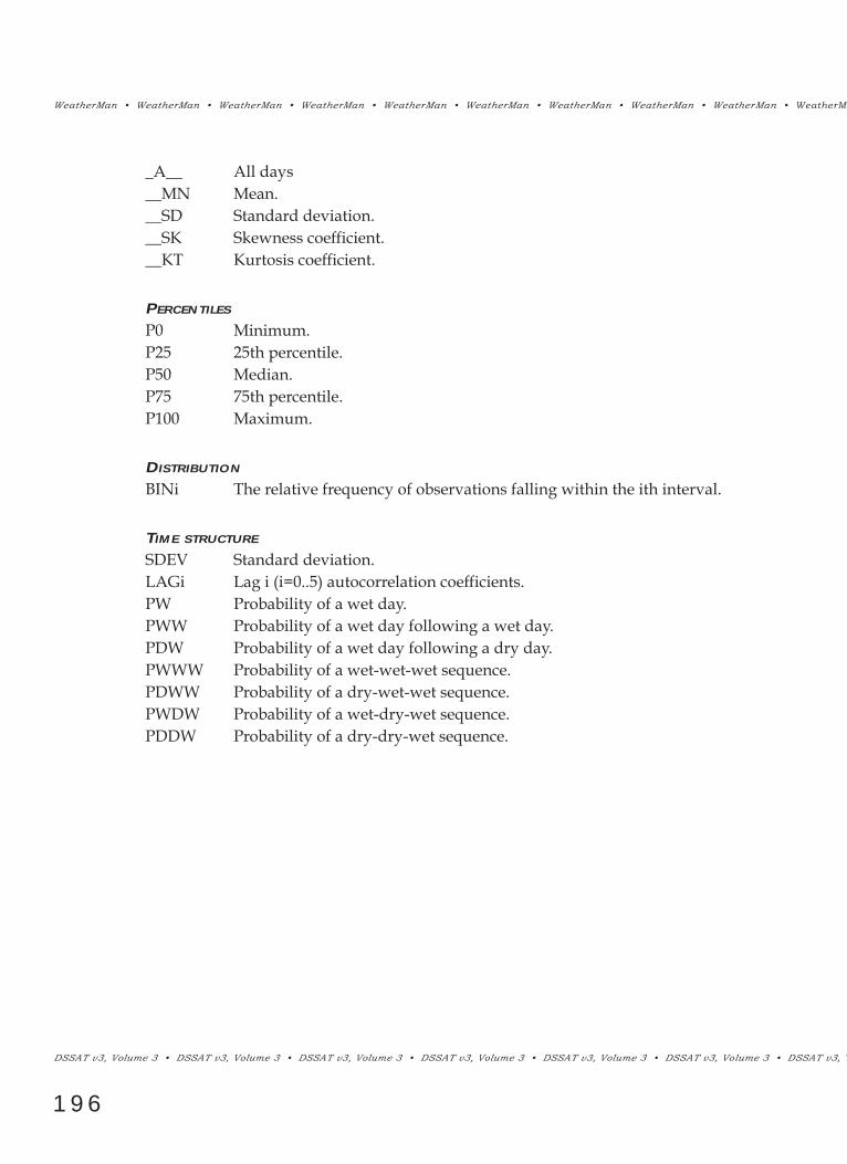
WeatherMan ¥ WeatherMan ¥ WeatherMan ¥ WeatherMan ¥ WeatherMan ¥ WeatherMan ¥ WeatherMan ¥ WeatherMan ¥ WeatherMan ¥ WeatherMa
DSSAT v3, Volume 3 ¥ DSSAT v3, Volume 3 ¥ DSSAT v3, Volume 3 ¥ DSSAT v3, Volume 3 ¥ DSSAT v3, Volume 3 ¥ DSSAT v3, Volume 3 ¥ DSSAT v3, V
196
_A__ All days__MN Mean.__SD Standard deviation.__SK Skewness coefficient.__KT Kurtosis coefficient.
PERCENTILES
P0 Minimum.P25 25th percentile.P50 Median.P75 75th percentile.P100 Maximum.
DISTRIBUTION
BINi The relative frequency of observations falling within the ith interval.
TIME STRUCTURE
SDEV Standard deviation.LAGi Lag i (i=0..5) autocorrelation coefficients.PW Probability of a wet day.PWW Probability of a wet day following a wet day.PDW Probability of a wet day following a dry day.PWWW Probability of a wet-wet-wet sequence.PDWW Probability of a dry-wet-wet sequence.PWDW Probability of a wet-dry-wet sequence.PDDW Probability of a dry-dry-wet sequence.

WeatherMan ¥ WeatherMan ¥ WeatherMan ¥ WeatherMan ¥ WeatherMan ¥ WeatherMan ¥ WeatherMan ¥ WeatherMan ¥ WeatherMan ¥ WeatherMan ¥
¥ DSSAT v3, Volume 3 ¥ DSSAT v3, Volume 3 ¥ DSSAT v3, Volume 3 ¥ DSSAT v3, Volume 3 ¥ DSSAT v3, Volume 3 ¥ DSSAT v3, Volume 3 ¥ DSSAT v3, Volume
197
The climate file contains summary information on a site in five sections. The*CLIMATE section contains characteristics of the location. The *MONTHLYAVERAGES section contains monthly means and Angstrom coefficients used bythe SIMMETEO weather generator. The *WGEN PARAMETERS section containsthe monthly distribution parameters used by the WGEN weather generator. The*RANGE CHECK VALUES section contains the values used to check for outliersand suspect data during the Import process. The *FLAGGED DATA COUNTsection contains counts of total, erroneous, and suspect data in the archive file.
*CLIMATE
LAT Latitude, degrees north.LONG Longitude, degrees east.ELEV Elevation, m.TAV Mean annual temperature, ¼C.AMP Half of the mean temperature difference between thewarmest and coolest month.SRAY Mean annual daily solar radiation, MJ/m2/day.TMXY Mean annual daily maximum temperature, ¼C.TMNY Mean annual daily minimum temperature, ¼C.RAIY Mean annual daily rainfall, mm.START Mean day of year of the first frost-free day.DURN Mean number of days between the last and the first frost.ANGA Intercept A in the Angstrom equation (Prescott, 1940).ANGB Multiplier B in the Angstrom equation (Prescott, 1940).REFHT Height of weather instruments above ground, m.WNDHT Height of annemometer above ground, m.GSST First year of observed weather data.GSDU Number of years of observed weather data.
APPENDIX B. CLIMATE FILE FORMAT

WeatherMan ¥ WeatherMan ¥ WeatherMan ¥ WeatherMan ¥ WeatherMan ¥ WeatherMan ¥ WeatherMan ¥ WeatherMan ¥ WeatherMan ¥ WeatherMa
DSSAT v3, Volume 3 ¥ DSSAT v3, Volume 3 ¥ DSSAT v3, Volume 3 ¥ DSSAT v3, Volume 3 ¥ DSSAT v3, Volume 3 ¥ DSSAT v3, Volume 3 ¥ DSSAT v3, V
198
*MONTHLY AVERAGES
MONTH Month (1 - January, 2 - February, etc.).SAMN Mean daily solar radiation for month, MJ/m2/day.XAMN Mean daily maximum temperature for month, ¼C.NAMN Mean daily minimum temperature for month, ¼C.RTOT Mean total rainfall for month, mm.RNUM Mean number of days with rainfall for month.SHMN Mean daily hours of bright sunshine for month, percent of
daylength.AMTH Intercept A in the Angstrom equation for month.BMTH Multiplier B in the Angstrom equation for month.
*WGEN PARAMETERS
MTH Month (1 - January, 2 - February, etc.).SDMN Mean daily solar radiation on dry days, MJ/m2/day.SDSD Standard deviation of solar radiation on dry days.SWMN Mean daily solar radiation on wet days, MJ/m2/day.SWSD Standard deviation of solar radiation on wet days.XDMN Mean daily maximum temperature on dry days, ¼C.XDSD Standard deviation of maximum temperature on dry days.XWMN Mean daily maximum temperature on wet days, ¼C.XWSD Standard deviation of maximum temperature on wet days.NAMN Mean daily minimum temperature, ¼C.NASD Standard deviation of minimum temperature.ALPHA Alpha coefficient of gamma distribution for rainfall.RTOT Total rainfall, mm.PDW Probability of a wet day following a dry day.RNUM Mean number of days with rainfall.
*RANGE CHECK VALUES
MIN Minimum value for range check.MAX Maximum value for range check.RATE Maximum change between days for range check.

WeatherMan ¥ WeatherMan ¥ WeatherMan ¥ WeatherMan ¥ WeatherMan ¥ WeatherMan ¥ WeatherMan ¥ WeatherMan ¥ WeatherMan ¥ WeatherMan ¥
¥ DSSAT v3, Volume 3 ¥ DSSAT v3, Volume 3 ¥ DSSAT v3, Volume 3 ¥ DSSAT v3, Volume 3 ¥ DSSAT v3, Volume 3 ¥ DSSAT v3, Volume 3 ¥ DSSAT v3, Volume
199
*FLAGGED DATA COUNT
BEGYR Year of first daily weather record.BEGDY Day of year of first daily weather record.ENDYR Year of last daily weather record.ENDDY Day of year of last daily weather record.TOTAL Total number of observations.VALID Number of observations without error flags.MISSING Number of missing values.ERROR Number of values with non-numeric strings encountered.ABOVE Number of values above the maximum.BELOW Number of values below the minimum.RATE Number of values with greater than maximum change from
previous day.

WeatherMan ¥ WeatherMan ¥ WeatherMan ¥ WeatherMan ¥ WeatherMan ¥ WeatherMan ¥ WeatherMan ¥ WeatherMan ¥ WeatherMan ¥ WeatherMa
DSSAT v3, Volume 3 ¥ DSSAT v3, Volume 3 ¥ DSSAT v3, Volume 3 ¥ DSSAT v3, Volume 3 ¥ DSSAT v3, Volume 3 ¥ DSSAT v3, Volume 3 ¥ DSSAT v3, V
200

L.A. HUNT,S. PARARAJASINGHAM
VO L U M E 3 -4
GENOTYPECOEFFICIENTCALCULATOR
UNIVERSITY OF GUELPH
INTERNATIONAL BENCHMARK SITES NETWORK FOR AGROTECHNOLOGY TRANSFER

Genotype Coefficient Calculator ¥ Genotype Coefficient Calculator ¥ Genotype Coefficient Calculator ¥ Genotype Coefficient Calculator ¥ Genotype Coeffi
DSSAT v3, Volume 3 ¥ DSSAT v3, Volume 3 ¥ DSSAT v3, Volume 3 ¥ DSSAT v3, Volume 3 ¥ DSSAT v3, Volume 3 ¥ DSSAT v3, Volume 3 ¥ DSSAT v3, V
202
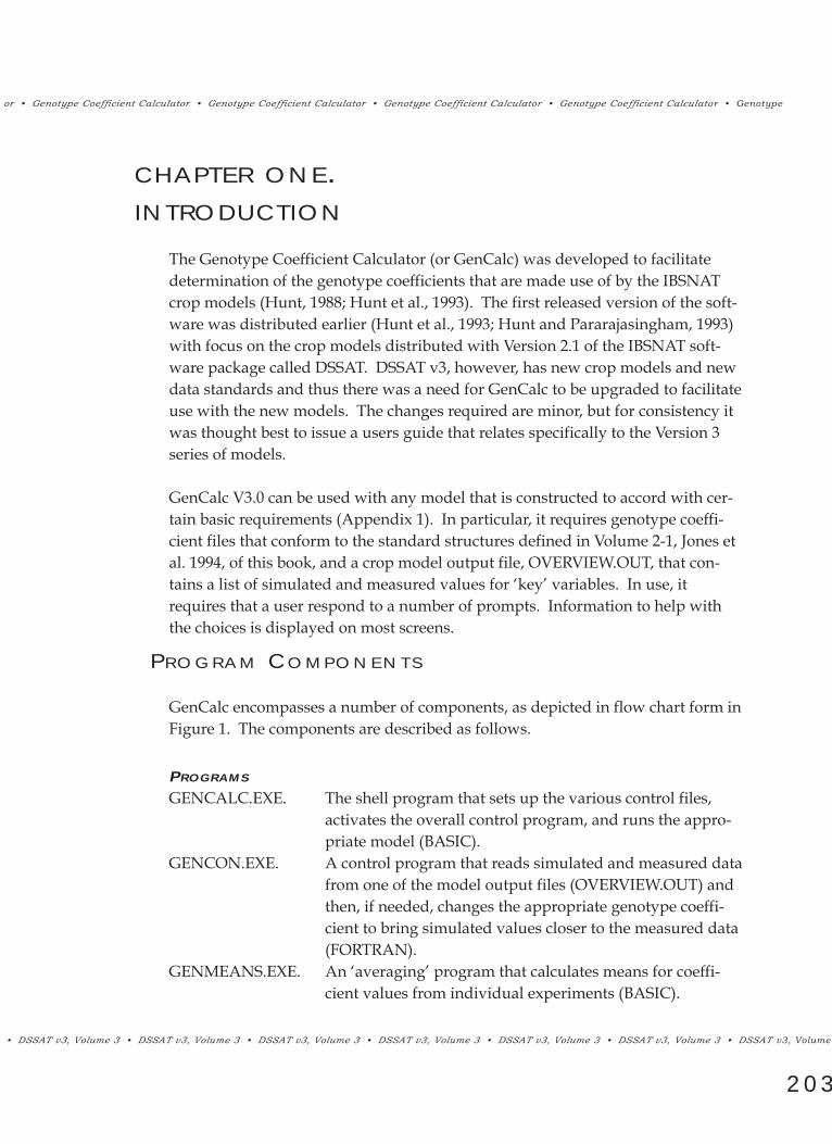
or ¥ Genotype Coefficient Calculator ¥ Genotype Coefficient Calculator ¥ Genotype Coefficient Calculator ¥ Genotype Coefficient Calculato r ¥ Genotype
¥ DSSAT v3, Volume 3 ¥ DSSAT v3, Volume 3 ¥ DSSAT v3, Volume 3 ¥ DSSAT v3, Volume 3 ¥ DSSAT v3, Volume 3 ¥ DSSAT v3, Volume 3 ¥ DSSAT v3, Volume
203
PR O G R A M CO M P O N E N T S
The Genotype Coefficient Calculator (or GenCalc) was developed to facilitatedetermination of the genotype coefficients that are made use of by the IBSNATcrop models (Hunt, 1988; Hunt et al., 1993). The first released version of the soft-ware was distributed earlier (Hunt et al., 1993; Hunt and Pararajasingham, 1993)with focus on the crop models distributed with Version 2.1 of the IBSNAT soft-ware package called DSSAT. DSSAT v3, however, has new crop models and newdata standards and thus there was a need for GenCalc to be upgraded to facilitateuse with the new models. The changes required are minor, but for consistency itwas thought best to issue a users guide that relates specifically to the Version 3series of models.
GenCalc V3.0 can be used with any model that is constructed to accord with cer-tain basic requirements (Appendix 1). In particular, it requires genotype coeffi-cient files that conform to the standard structures defined in Volume 2-1, Jones etal. 1994, of this book, and a crop model output file, OVERVIEW.OUT, that con-tains a list of simulated and measured values for ÔkeyÕ variables. In use, itrequires that a user respond to a number of prompts. Information to help withthe choices is displayed on most screens.
CHAPTER ONE.INTRODUCTION
GenCalc encompasses a number of components, as depicted in flow chart form inFigure 1. The components are described as follows.
PROGRAMS
GENCALC.EXE. The shell program that sets up the various control files,activates the overall control program, and runs the appro-priate model (BASIC).
GENCON.EXE. A control program that reads simulated and measured datafrom one of the model output files (OVERVIEW.OUT) andthen, if needed, changes the appropriate genotype coeffi-cient to bring simulated values closer to the measured data(FORTRAN).
GENMEANS.EXE. An ÔaveragingÕ program that calculates means for coeffi-cient values from individual experiments (BASIC).
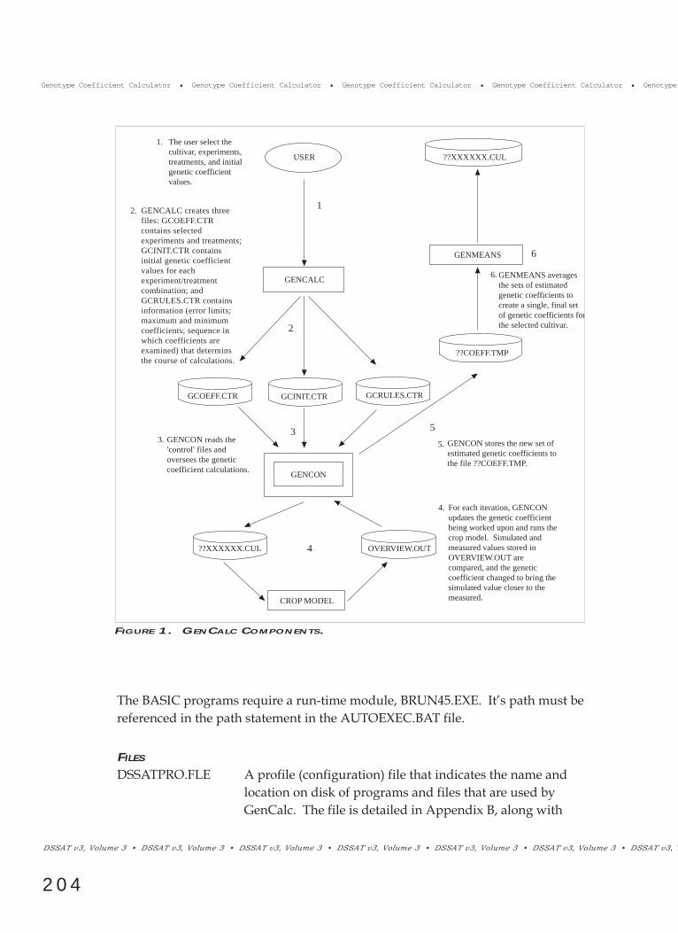
The BASIC programs require a run-time module, BRUN45.EXE. ItÕs path must bereferenced in the path statement in the AUTOEXEC.BAT file.
FILES
DSSATPRO.FLE A profile (configuration) file that indicates the name andlocation on disk of programs and files that are used byGenCalc. The file is detailed in Appendix B, along with
Genotype Coefficient Calculator • Genotype Coefficient Calculator • Genotype Coefficient Calculator • Genotype Coefficient Calculator • Genotype
DSSAT v3, Volume 3 ¥ DSSAT v3, Volume 3 ¥ DSSAT v3, Volume 3 ¥ DSSAT v3, Volume 3 ¥ DSSAT v3, Volume 3 ¥ DSSAT v3, Volume 3 ¥ DSSAT v3, V
204
CROP MODEL
??XXXXXX.CUL OVERVIEW.OUT
GENCON
GCOEFF.CTR GCINIT.CTR GCRULES.CTR
GENCALC
??COEFF.TMP
GENMEANS
??XXXXXX.CUL
The user select the cultivar, experiments, treatments, and initial genetic coefficient values.
USER
GENCON reads the 'control' files and oversees the genetic coefficient calculations.
For each iteration, GENCON updates the genetic coefficient being worked upon and runs the crop model. Simulated and measured values stored in OVERVIEW.OUT are compared, and the genetic coefficient changed to bring the simulated value closer to the measured.
GENCON stores the new set of estimated genetic coefficients to the file ??COEFF.TMP.
5.
4.
GENMEANS averages the sets of estimated genetic coefficients to create a single, final set of genetic coefficients forthe selected cultivar.
6.
1.
3.
1
2
3 5
4
6
GENCALC creates three files: GCOEFF.CTR contains selected experiments and treatments; GCINIT.CTR contains initial genetic coefficient values for each experiment/treatment combination; and GCRULES.CTR contains information (error limits; maximum and minimum coefficients; sequence in which coefficients are examined) that determins the course of calculations.
2.
FIGURE 1. GENCALC COMPONENTS.

or ¥ Genotype Coefficient Calculator ¥ Genotype Coefficient Calculator ¥ Genotype Coefficient Calculator ¥ Genotype Coefficient Calculato r ¥ Genotype
¥ DSSAT v3, Volume 3 ¥ DSSAT v3, Volume 3 ¥ DSSAT v3, Volume 3 ¥ DSSAT v3, Volume 3 ¥ DSSAT v3, Volume 3 ¥ DSSAT v3, Volume 3 ¥ DSSAT v3, Volume
205
procedures for making changes to it. In DSSAT v3, GenCalcis located in directory C:\DSSAT3. For stand-alone use, thedirectory in which it is located could be chosen at the userÕsdiscretion. In all cases, however, the directory must be refer-enced by adding a ÔSETÕ statement to the AUTOEXEC.BATfile. For a C:\DSSAT3 location, the required statementwould be: SET DSSAT3 = C:\DSSAT3.
GCRULES.FLE A file containing the rules that govern the sequence of geno-type coefficient calculations for different crops. This file canbe located in any directory, but the directory must be refer-enced in the configuration file. Contents of the file arecopied to a temporary file (GCRULES.CTR) that is used dur-ing computation.
??COEFF.TMP and ENDPOINT.TMP Files generated internally at each new model run. The ??
indicates a crop code such as ÔWHÕ for wheat. The calculatedgenotype coefficient values are stored in ??COEFF.TMPwhile end point information (simulated and measured val-ues at completion) is stored in ENDPOINT.TMP for eachcoefficient. Information in these files is displayed for perusalat the completion of a genotype coefficient calculation ses-sion.
REQUIREMENTS
In DSSAT v3, the file designated as FILEA required in addition to those which arenecessary for running the DSSAT v3 models. The naming convention for these filesand for FILEA is described in Volume 2-1, Jones et al. 1994, of this book. FILEAcontains experimental data used to determine the goodness-of-fit of simulatedresults. The following data must be present in FILEA:
Peanut: Flowering dateMaturity dateSeed yieldBiomass at maturitySeed number/m2
Seed number per podSeed dry weightFirst pod dateFull pod datePod yield (dry)

Genotype Coefficient Calculator ¥ Genotype Coefficient Calculator ¥ Genotype Coefficient Calculator ¥ Genotype Coefficient Calculator ¥ Genotype Coeffi
DSSAT v3, Volume 3 ¥ DSSAT v3, Volume 3 ¥ DSSAT v3, Volume 3 ¥ DSSAT v3, Volume 3 ¥ DSSAT v3, Volume 3 ¥ DSSAT v3, Volume 3 ¥ DSSAT v3, V
206
Maize: Silking dateMaturity dateGrain yield (dry)Biomass at maturityGrain number/m2
Grain number per earGrain weight (dry)
Soybean: Flowering dateMaturity dateGrain yieldBiomass at maturity (no leaves)Grain number/m2
Grain number per podGrain dry weight
Wheat: Anthesis dateMaturity dateGrain yield (dry)Biomass at maturityGrain number/m2
Grain number per spikeGrain weight (dry)
The files that contain the genotype coefficients for the models used with the cal-culator are named as ??XXXYY0.CUL, where Ò??Ó is the crop identification code,ÒXXXÓ is the model abbreviation and ÒYYÓ is the version number of the model.Genotype coefficient values calculated from model runs, at the userÕs discretion,may be entered into this cultivar file. As described under the GenCalc operation(see Step 5 in Chapter 4), the genotype coefficient values from the cultivar file arecopied to the GCINIT.CTR file for display as initial values for the genotype inquestion. (The GCINIT.CTR file is explained in Figure 1). For the case where agenotype that is not present in the cultivar file is included in an experiment, theuser must use an editor to enter into the cultivar file a unique number and nameand an initial ÔguessÕ at the genotype coefficients.

or ¥ Genotype Coefficient Calculator ¥ Genotype Coefficient Calculator ¥ Genotype Coefficient Calculator ¥ Genotype Coefficient Calculato r ¥ Genotype
¥ DSSAT v3, Volume 3 ¥ DSSAT v3, Volume 3 ¥ DSSAT v3, Volume 3 ¥ DSSAT v3, Volume 3 ¥ DSSAT v3, Volume 3 ¥ DSSAT v3, Volume 3 ¥ DSSAT v3, Volume
207
GenCalc will run on any IBM or IBM-compatible computer with MS-DOS v3.0and later. A hard disk drive with approximately 2 Mb free disk space is required.For stand-alone installation, GenCalc requires the creation (if not already present)of a directory C:\DSSAT3. The DSSATPRO.FLE described in the Componentssection of this guide and Appendix B must be placed in this directory. GenCalcalso uses a number of subdirectories under C:\DSSAT3, namely GENOTYPE,PEANUT, SOYBEAN, and WHEAT. The GenCalc component programs togetherwith the crop model executable programs are placed in the DSSAT3 subdirectory,while the crop model input files are placed in subdirectories named after the cropin question. Model and crop specific genotype coefficients files (??XXXYY0.CULfiles) and the GCRULES.FLE are placed in the GENOTYPE subdirectory. Allcould be changed, as long as the location of the configuration file(DSSATPRO.FLE) remains the same as that of the program executables.
SY S T E M RE Q U I R E M E N T S

Genotype Coefficient Calculator ¥ Genotype Coefficient Calculator ¥ Genotype Coefficient Calculator ¥ Genotype Coefficient Calculator ¥ Genotype Coeffi
DSSAT v3, Volume 3 ¥ DSSAT v3, Volume 3 ¥ DSSAT v3, Volume 3 ¥ DSSAT v3, Volume 3 ¥ DSSAT v3, Volume 3 ¥ DSSAT v3, Volume 3 ¥ DSSAT v3, V
208

or ¥ Genotype Coefficient Calculator ¥ Genotype Coefficient Calculator ¥ Genotype Coefficient Calculator ¥ Genotype Coefficient Calculato r ¥ Genotype
¥ DSSAT v3, Volume 3 ¥ DSSAT v3, Volume 3 ¥ DSSAT v3, Volume 3 ¥ DSSAT v3, Volume 3 ¥ DSSAT v3, Volume 3 ¥ DSSAT v3, Volume 3 ¥ DSSAT v3, Volume
209
CHAPTER TWO.GETTING STARTED
GenCalc can be run from the DSSAT v3 Shell or as a stand-alone program. (SeeVolume 1-3, Hunt et al. 1994b, of this book for a description of the Shell.) Fromthe DSSAT v3 Shell, open the DATA main menu, select ÒGenotypeÓ from themenu (see Screen 1, below) and then select ÒCalculateÓ from the submenu pre-sented. The first screen of the GenCalc program (Screen 3) will be presented.
To run GenCalc as a stand-alone program, refer to Hunt and Pararajasingham(1994).
Transfer experiment data sets with genotypes you wish to examine into theappropriate directory (e.g., wheat data into C:\DSSAT3\WHEAT), and use aneditor to add the experiment(s) to the list in the EXP.LST file. (See Appendix Afor an example of this file and Volume 2-1, Jones et al. 1994, for this book for adescription of this file.) These data sets must be complete with weather and soilsdata and with data in the cultivar file.
B BackgroundX ExperimentG GenotypeW WeatherS SoilP PestE Economic
DECISION SUPPORT SYSTEM FOR AGROTECHNOLOGY TRANSFER
DATA MODEL ANALYSES TOOLS SETUP/QUIT
ESCmoves through menu choicesmoves to higher menu level Version: 3.0
↑ ↓ → ←
Cultivar, ecotype, and species information.
SCREEN 1.

Genotype Coefficient Calculator ¥ Genotype Coefficient Calculator ¥ Genotype Coefficient Calculator ¥ Genotype Coefficient Calculator ¥ Genotype Coeffi
DSSAT v3, Volume 3 ¥ DSSAT v3, Volume 3 ¥ DSSAT v3, Volume 3 ¥ DSSAT v3, Volume 3 ¥ DSSAT v3, Volume 3 ¥ DSSAT v3, Volume 3 ¥ DSSAT v3, V
210

or ¥ Genotype Coefficient Calculator ¥ Genotype Coefficient Calculator ¥ Genotype Coefficient Calculator ¥ Genotype Coefficient Calculato r ¥ Genotype
¥ DSSAT v3, Volume 3 ¥ DSSAT v3, Volume 3 ¥ DSSAT v3, Volume 3 ¥ DSSAT v3, Volume 3 ¥ DSSAT v3, Volume 3 ¥ DSSAT v3, Volume 3 ¥ DSSAT v3, Volume
211
When GenCalc is opened from the DSSAT v3 Shell DATA main menu, Screen 2(below) is presented. Follow the procedure in the steps listed below to determinethe coefficients for one genotype. This procedure is often followed in determiningcoefficients, but it is not the only one. It should thus be viewed as a starting point,not as a fixed recipe. Users may develop a different approach, as experience isgained, or they may miss some steps. Users should also be aware that some errorsmay cause the software to enter an endless loop. Should this appear to happen,turn off the computer or re-boot by pressing <CTR>-<ALT>-<DEL>.
CHAPTER THREE.RUNNING GENCALC
GENOTYPE COEFFICIENT CALCULATOR VERSION : 3
The calculator can be used to determine coefficients for individual treatments, or to calculate averages from previous determinations.
PRESS
'I' for INDIVIDUAL determinations
'A' for AVERAGES calculations
'Q' to QUIT
NB Please ensure that any datasets to be used are 'model tested'.
Determine genotype coefficients for one or more experiments; calculate average values after determining coefficients for several experiments.
SCREEN 2.
DE T E R M I N E GE N E T I C CO E F F I C I E N T S
1. In Screen 2, press the <I> key. This directs the genotype coefficient calculatorto determine values for specific experiment/treatment combinations.
2. Select a crop in Screen 3 (on following page) for the genotype you wish to cal-culate
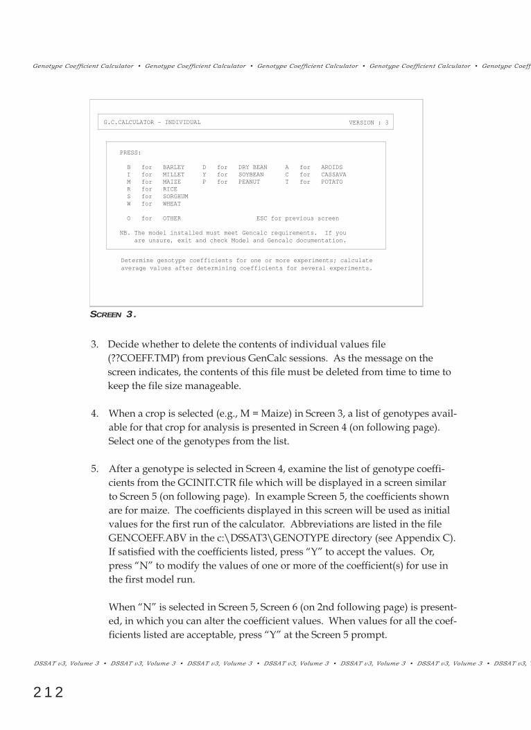
Genotype Coefficient Calculator ¥ Genotype Coefficient Calculator ¥ Genotype Coefficient Calculator ¥ Genotype Coefficient Calculator ¥ Genotype Coeffi
DSSAT v3, Volume 3 ¥ DSSAT v3, Volume 3 ¥ DSSAT v3, Volume 3 ¥ DSSAT v3, Volume 3 ¥ DSSAT v3, Volume 3 ¥ DSSAT v3, Volume 3 ¥ DSSAT v3, V
212
3. Decide whether to delete the contents of individual values file(??COEFF.TMP) from previous GenCalc sessions. As the message on thescreen indicates, the contents of this file must be deleted from time to time tokeep the file size manageable.
4. When a crop is selected (e.g., M = Maize) in Screen 3, a list of genotypes avail-able for that crop for analysis is presented in Screen 4 (on following page).Select one of the genotypes from the list.
5. After a genotype is selected in Screen 4, examine the list of genotype coeffi-cients from the GCINIT.CTR file which will be displayed in a screen similarto Screen 5 (on following page). In example Screen 5, the coefficients shownare for maize. The coefficients displayed in this screen will be used as initialvalues for the first run of the calculator. Abbreviations are listed in the fileGENCOEFF.ABV in the c:\DSSAT3\GENOTYPE directory (see Appendix C).If satisfied with the coefficients listed, press ÒYÓ to accept the values. Or,press ÒNÓ to modify the values of one or more of the coefficient(s) for use inthe first model run.
When ÒNÓ is selected in Screen 5, Screen 6 (on 2nd following page) is present-ed, in which you can alter the coefficient values. When values for all the coef-ficients listed are acceptable, press ÒYÓ at the Screen 5 prompt.
G.C.CALCULATOR - INDIVIDUAL VERSION : 3
PRESS:
B for BARLEY D for DRY BEAN A for AROIDS I for MILLET Y for SOYBEAN C for CASSAVA M for MAIZE P for PEANUT T for POTATO R for RICE S for SORGHUM W for WHEAT
O for OTHER ESC for previous screen
NB. The model installed must meet Gencalc requirements. If you
Determine genotype coefficients for one or more experiments; calculate average values after determining coefficients for several experiments.
are unsure, exit and check Model and Gencalc documentation.
SCREEN 3.

or ¥ Genotype Coefficient Calculator ¥ Genotype Coefficient Calculator ¥ Genotype Coefficient Calculator ¥ Genotype Coefficient Calculato r ¥ Genotype
¥ DSSAT v3, Volume 3 ¥ DSSAT v3, Volume 3 ¥ DSSAT v3, Volume 3 ¥ DSSAT v3, Volume 3 ¥ DSSAT v3, Volume 3 ¥ DSSAT v3, Volume 3 ¥ DSSAT v3, Volume
213
6. In the next dialog box presented, respond with an ÒNÓ to the prompt,ÔCalculate ALL coefficients?Õ. And at the next prompt, respond with a ÒYÓ tocalculate only the DEVELOPMENT (those concerned with the duration ofthe life cycle) coefficients.
7. Screen 7 (on following page) will be presented which lists experiments which
G.C.CALCULATOR - INDIVIDUAL VERSION : 3
CROP: Maize MODEL: GECER930
Generally, the displayed coefficients should be used for the first run;changed for susequent runs. This helps in obtaining multi-site fits.
Current coefficients are: P1 P2 P5 G2 G3 PHINT1 2 3 4 5 6320. .520 940. 625. 6.00 75.0Use these for first simulation of new run ?
Press : Y or N
SCREEN 5.
G.C.CALCULATOR - INDIVIDUAL VERSION : 3
CROP: Maize MODEL: GECER930
Determine genotype coefficients for one or more experiments; calculate average values after determining coefficients for several experiments.
No Name 1 PIO 3382 2 McCurdy 84aa 3 H610(UH) 4 PIO x 304C
Enter NUMBER to select genotype: press ENTER for previous screen --->
SCREEN 4.
Genotype Coefficient Calculator ¥ Genotype Coefficient Calculator ¥ Genotype Coefficient Calculator ¥ Genotype Coefficient Calculator ¥ Genotype Coeffi
DSSAT v3, Volume 3 ¥ DSSAT v3, Volume 3 ¥ DSSAT v3, Volume 3 ¥ DSSAT v3, Volume 3 ¥ DSSAT v3, Volume 3 ¥ DSSAT v3, Volume 3 ¥ DSSAT v3, V
214
include the selected genotype. Choose experiments to be used for genotype coef-ficient calculation by typing either ÒYÓ or ÒNÓ to the prompt for each experiment.
8. The treatments for each experiment selected will be displayed in Screen 8 (on fol-lowing page). Choose all or some treatment(s) in the chosen experiments for geno-type coefficient calculation by responding appropriately (ÒYÓ or ÒNÓ) to theprompts on the screen.
G.C.CALCULATOR - INDIVIDUAL VERSION : 3
CROP: Maize MODEL: GECER940
Generally, the displayed coefficients should be used for the first run;changed for subsequent runs. This helps in obtaining multi-site fits.
Current coefficients are: P1 P2 P5 G2 G4 PHINT1 2 3 4 5 6320. .520 940. 625. 6.00 75.0Which coefficient to change ?ENTER 1,2 etc. -->
SCREEN 6.
G.C.CALCULATOR - INDIVIDUAL VERSION : 3
CROP: Maize MODEL: GECER940
Generally it is preferable to work first with few experiments and/ortreatments, then to proceed using the coefficients so determined.
The selected genotype was included in experiment: IBWA8301
Accept this experiment ?
Press : Y or N
SCREEN 7.
or ¥ Genotype Coefficient Calculator ¥ Genotype Coefficient Calculator ¥ Genotype Coefficient Calculator ¥ Genotype Coefficient Calculato r ¥ Genotype
¥ DSSAT v3, Volume 3 ¥ DSSAT v3, Volume 3 ¥ DSSAT v3, Volume 3 ¥ DSSAT v3, Volume 3 ¥ DSSAT v3, Volume 3 ¥ DSSAT v3, Volume 3 ¥ DSSAT v3, Volume
215
9. In the dialog box next presented, type an ÒNÓ at the prompt, ÔSelection ofruns for this genotype complete?Õ because you want to set up anothersequence of calculation for the genotype in question but with different initialcoefficients.
Screen 5 will again be presented (see Step 5). Change one of the coefficient(s)by 20 to 30% as described under Step 5.
When the prompt ÔSelection of runs for this genotype complete?Õ reappears,respond with ÒNÓ again to bring up the initial genotype coefficients list, butthis time decrease the appropriate coefficient by 10 to 20%.
NOTE: Setting an array of initial values for particular coefficient(s) is necessary todevelop data for examination of variation in the values fitted for the varying coeffi-cient(s).
10. Now at the prompt, ÔSelection of runs for this genotype complete?Õ, typeÒYÓto proceed with the genotype coefficient calculation. The calculator willrun the appropriate crop model, and data indicating the goodness-of-fitbetween predicted and actual data will be displayed on the screen as calcula-tions proceed. For each set of calculations, final coefficient values and endpoint information are stored in files (??COEFF.TMP and ENDPOINT.TMP,respectively) so that these are available for subsequent viewing.
G.C.CALCULATOR - INDIVIDUAL VERSION : 3
CROP: Maize MODEL: GECER940
Generally it is preferable to work first with few experiments and/ortreatments, then to proceed using the coefficients so determined.
The selected genotype was included in experiments: IBWA8301....... in the following treatments:
1 2 3
Accept all treatments ? Press : Y or N
SCREEN 8.

Genotype Coefficient Calculator ¥ Genotype Coefficient Calculator ¥ Genotype Coefficient Calculator ¥ Genotype Coefficient Calculator ¥ Genotype Coeffi
DSSAT v3, Volume 3 ¥ DSSAT v3, Volume 3 ¥ DSSAT v3, Volume 3 ¥ DSSAT v3, Volume 3 ¥ DSSAT v3, Volume 3 ¥ DSSAT v3, Volume 3 ¥ DSSAT v3, V
216
11. When calculations are completed, press the <C> key in Screen 9 (above) toview the array of coefficients calculated for each set of calculations in the??COEFF.TMP file (Screen 10, below). While viewing these final coefficientvalues, pay particular attention to the codes assigned by GenCalc, if at all, toeach of the calculated genotype coefficients (see Appendix C for a descriptionof these codes). Growth coefficients will have a ÒUÓ immediately followingthe numerical value. This indicates that the particular coefficient was not
*MAIZE COEFFICIENTS
@NGENO EXPMENT R RUN T ETYPE P1 P2 P5 G2 G3 PHINTIB0063 IBSI8001 2 1 1 IB0001 320.D.5200D 940.D 625.U6.000U75.00UIB0063 IBSI8001 2 1 2 IB0001 320.D.5200D 940.D 625.U6.000U75.00UIB0063 IBWA8301 2 1 1 IB0001 340. .5200M 940.M 625.U6.000U75.00UIB0063 IBWA8301 2 1 2 IB0001 340. .5200M 940.M 625.U6.000U75.00UIB0063 IBWA8301 2 1 3 IB0001 340. .5200 940.M 625.U6 000U75.00U
SCREEN 10.
G.C.CALCULATOR - INDIVIDUAL VERSION : 3
CROP: Maize MODEL: GECER930
All calculations completed ...
PRESS: C to view COEFFICIENTS E to view END POINTS O to view OUTPUTS
A to calculate AVERAGES
ENTER to proceed to the next menu
It is generally desirable to examine the endpoints. If the fit wasnot good, the process should be repeated with new initial values.
SCREEN 9.

or ¥ Genotype Coefficient Calculator ¥ Genotype Coefficient Calculator ¥ Genotype Coefficient Calculator ¥ Genotype Coefficient Calculato r ¥ Genotype
¥ DSSAT v3, Volume 3 ¥ DSSAT v3, Volume 3 ¥ DSSAT v3, Volume 3 ¥ DSSAT v3, Volume 3 ¥ DSSAT v3, Volume 3 ¥ DSSAT v3, Volume 3 ¥ DSSAT v3, Volume
217
SCREEN 11.
determined during the iterative calculations of the current session. Theremaining coefficients should have no associated letter. If this is the case,press the exit key of your editor and proceed to Step 12. If, however, thedevelopment coefficients were associated with a letter, which may occurwhen the initial coefficients were either close to the maximum/minimum val-ues, or were considerably different from the real values, proceed through thefollowing steps:
11a. Screen 10 shows an an example ??COEFF.TMP file for maize. Make a noteof the letter and the coefficient value for each coefficient listed which has aletter. The letter ÒMÓ indicates that the calculated coefficient reached themaximum or minimum value defined in the GCRULES.FLE file, while anÒRÓ indicates that the maximum number of runs specified in theGCRULES.FLE file was reached before an acceptable end point was reached.Other codes that may appear are defined in Appendix C.
11b. Exit Screen 10 by pressing the <F7> key if using the editor (TVED.EXE) dis-tributed with DSSAT v3. If you are using an editor of choice, use therequired key to exit the screen. You will be returned to Screen 9.
11c. Now in Screen 9, press the <E> key to view the end-points in the END-POINT.TMP file (see Screen 11, below). For each coefficient with an associat-ed letter noted in Screen 10, make a note as to whether the simulated value isgreater or less than the measured value.
*GENOTYPE COEFFICIENT CALCULATION - END POINT COMPARISONS.
EXPERIMENT TRTMT COEFF NAME SIMULATED MEASURED REFERENCE TRAIT(S)
IBSI8001 1 3 DESP (P2) 61.000 .000 SILKING DATE IBSI8001 1 1 DUJU (P1) 61.000 .000 SILKING DATE IBSI8001 1 2 DUGF (P5) 111.000 .000 MATURITY DATE IBSI8001 2 3 DESP (P2) 61.000 .000 SILKING DATE IBSI8001 2 1 DUJU (P1) 61.000 .000 SILKING DATE IBSI8001 2 2 DUGF (P5) 111.000 .000 MATURITY DATE IBWA8301 1 3 DESP (P2) 76.000 79.000 SILKING DATE IBWA8301 1 1 DUJU (P1) 78.000 79.000 SILKING DATE IBWA8301 1 2 DUGF (P5) 137.000 139.000 MATURITY DATE IBWA8301 2 3 DESP (P2) 76.000 79.000 SILKING DATE IBWA8301 2 1 DUJU (P1) 78.000 79.000 SILKING DATE IBWA8301 2 2 DUGF (P5) 137.000 135.000 MATURITY DATE IBWA8301 3 3 DESP (P2) 76.000 78.000 SILKING DATE IBWA8301 3 1 DUJU (P1) 78.000 78.000 SILKING DATE IBWA8301 3 2 DUGF (P5) 137.000 136.000 MATURITY DATE
F1ABORT F2UNDO F3PRINT F4MARK F5CUT F6PASTE F7EXIT F8DEL EOL F9DEL L F10UDEL L I
Genotype Coefficient Calculator ¥ Genotype Coefficient Calculator ¥ Genotype Coefficient Calculator ¥ Genotype Coefficient Calculator ¥ Genotype Coeffi
DSSAT v3, Volume 3 ¥ DSSAT v3, Volume 3 ¥ DSSAT v3, Volume 3 ¥ DSSAT v3, Volume 3 ¥ DSSAT v3, Volume 3 ¥ DSSAT v3, Volume 3 ¥ DSSAT v3, V
218
11d. Exit Screen 11 by pressing the <F7> key. You will again be returned to Screen9.
11e. Press the <ENTER> key in Screen 9 to continue.
11f. Screen 12 (below) will be presented. Press the <G> key to return to the geno-type selection screen (Screen 4).
11g. Choose the same genotype as selected before in Screen 4.
11h. If the letter from the??COEFF.TMP file (Screen 10) for a coefficient was an ÒR,Órespond with an ÒNÓ to the prompt, ÔUse these for first simulation of newrun?Õ. Then in the dialog box which appears, change the value for the appro-priate coefficient. Increase the value by approximately 30% if the simulatedvalue was less than the measured; decrease the value similarly if the inverse.Then proceed as from Step 6.
If the letter was an ÒM,Ó proceed as from Step 5, but when the CoefficientSelection screen (Screen 6) is reached, press the <ENTER> key and edit therules file. For the coefficient(s) in question, reduce the minimum (MNCEF) orincrease the maximum (MXCEF) for rule set 2 of the crop in question, depend-ing on whether the coefficient value noted in Step 11a was near the minimumor maximum. Then exit the rules file and proceed as indicated in Step 6.
G.C.CALCULATOR - INDIVIDUAL VERSION : 3
PRESS:
G to select more GENOTYPES
C to select another CROP
ENTER to return to the main menu
Determine genotype coefficients for one or more experiments; calculate average values after determining coefficients for several experiments.
SCREEN 12.

or ¥ Genotype Coefficient Calculator ¥ Genotype Coefficient Calculator ¥ Genotype Coefficient Calculator ¥ Genotype Coefficient Calculato r ¥ Genotype
¥ DSSAT v3, Volume 3 ¥ DSSAT v3, Volume 3 ¥ DSSAT v3, Volume 3 ¥ DSSAT v3, Volume 3 ¥ DSSAT v3, Volume 3 ¥ DSSAT v3, Volume 3 ¥ DSSAT v3, Volume
219
12. If the coefficient calculations proceeded to completion satisfactorily, pressthe <ENTER> key and you will be prompted in the next screen for selectionof another genotype of the same crop, for the selection of another crop, orfor return to the main menu. Press the <ENTER> key to return to theGenCalc main menu (Screen 2), and once within the main menu, press ÒAÓfor the calculation of average coefficients from previous determinations.Selecting ÒAÓ allows you to calculate the AVERAGES of coefficients calculat-ed from various experiments using the Steps above. If desired, you mayreplace coefficient values in the cultivar file with these values (see Step 20).
13. The calculator will then prepare a list of coefficients calculated for the geno-type in question in previous specific experiment/treatment runs (Screen 13,below). Each of these runs is assigned a sequence number in the listing (RUNcolumn) as shown in Screen 10, along with a number denoting whether all(1), development (2) or growth (3) coefficients were determined (R column).A column headed with a ÒTÓ contains the number of the treatment used forthe particular set of coefficient calculations.
14. In Screen 13, select a run number. Once a run number is chosen, mean coeffi-cients are calculated from individual values obtained for different experi-ments and treatments but with the same initial coefficient values, along withtheir respective coefficients of variation. These values are displayed, together
G.C.CALCULATOR - AVERAGES VERSION : 3
CODE EXPMENT R RUN T ETYPE P1 P2 P5 G2 G3 PHINTIB0063 IBSI8001 2 1 1 IB0001 320.D.5200D 940.D 625.U6.000U75.00UIB0063 IBSI8001 2 1 1 IB0001 320.D.5200D 940.D 625.U6.000U75.00UIB0063 IBSI8001 2 2 1 IB0001 320.D.5200D 940.D 625.U6.000U75.00UIB0063 IBSI8001 2 2 2 IB0001 320.D.5200D 940.D 625.U6.000U75.00UIB0063 IBWA8301 2 1 1 IB0001 340. .5200M 940.M 625.U6.000U75.00UIB0063 IBWA8301 2 1 2 IB0001 340. .5200M 940.M 625.U6.000U75.00UIB0063 IBWA8301 2 1 3 IB0001 340. .5200M 940.M 625.U6.000U75.00UIB0063 IBWA8301 2 2 1 IB0001 340. .5200M 940.M 625.U6.000U75.00UIB0063 IBWA8301 2 2 2 IB0001 340. .5200M 940.M 625.U6.000U75.00UIB0063 IBWA8301 2 2 3 IB001 340. .5200 940.M 625.U6.000U75.00U
Which RUN to select ? [ Enter number from RUN column ] -->
Main coefficients for different experiments and initial values.Initial values are referenced in the 'Run' column. T=treatments.
SCREEN 13.

Genotype Coefficient Calculator ¥ Genotype Coefficient Calculator ¥ Genotype Coefficient Calculator ¥ Genotype Coefficient Calculator ¥ Genotype Coeffi
DSSAT v3, Volume 3 ¥ DSSAT v3, Volume 3 ¥ DSSAT v3, Volume 3 ¥ DSSAT v3, Volume 3 ¥ DSSAT v3, Volume 3 ¥ DSSAT v3, Volume 3 ¥ DSSAT v3, V
220
with values currently in the cultivar file, in Screen 14 (above). Coefficientsthat were not estimated, or for which calculations were terminated before anacceptable end-point was reached, are displayed as zeros. These coefficientswould have had a letter associated with them in the ??COEFF.TMP file (seeStep 11).
15. In the dialog box at the bottom of Screen 14, press ÒYÓ to select an additionalrun.
16. Press ÒYÓ again when the second set of coefficients has been calculated. PressÒYÓ and Ò3Ó to select results from the third run.
17. This time press ÒNÓ at the prompt in Screen 14 to indicate that run selection iscomplete.
18. At this stage a list of standard deviations for coefficients in the different runsis presented. Select the one with the lowest standard deviation for the ÔtargetÕcoefficient.
19. A list of ÔnewÕ and ÔoldÕ mean coefficient values is now displayed. In this list,coefficients that were not calculated will have been replaced by those in thecultivar file. Press ÒYÓ at the prompt to accept all values.
G.C.CALCULATOR - AVERAGES VERSION : 3
GENOTYPE: P10 X 304C 1 2 3 4 5 6 P1 P2 P5 G2 G3 PHINTOld values: 320. .520 940. 625. 6.00 75.0New vlues: 340. .520 .000 .000 .000 .000C.V.'s: 0 0 0 0 0 0
Treatments: 3 1 0 0 0 0
Number of experiments : 1
SELECT an additional run ? [ PRESS Y or N ]
Coefficient values determined for differnet experiments and one setof initial values. Coefficients of variation if more than 3 values.
SCREEN 14.

or ¥ Genotype Coefficient Calculator ¥ Genotype Coefficient Calculator ¥ Genotype Coefficient Calculator ¥ Genotype Coefficient Calculato r ¥ Genotype
¥ DSSAT v3, Volume 3 ¥ DSSAT v3, Volume 3 ¥ DSSAT v3, Volume 3 ¥ DSSAT v3, Volume 3 ¥ DSSAT v3, Volume 3 ¥ DSSAT v3, Volume 3 ¥ DSSAT v3, Volume
221
20. Respond with a ÒYÓ to the prompt asking whether or not to replace the ÔoldÕvalues in the cultivar file.
21. Respond with an ÒNÓ to the prompt asking if you wish to edit the cultivarfile, although including notes in the cultivar file may be useful for future ref-erence.
22. At this stage, the process should be repeated from Step 1 to calculate thegrowth coefficients for the cultivar in question. Exit the averaging programand press the <ENTER> key to display the prompts to select another geno-type or a different crop. Press the <G> key to select a genotype and repeatthe process.
23. Respond with an ÒNÓ response to the prompt ÒCalculate DEVELOPMENTcoefficients only.Ó Follow this by a ÒYÓ response to the prompt ÒCalculateGROWTH coefficients onlyÓ in Step 6. Continue with Step 7.
Repeat the process for the GROWTH coefficients. Upon completion, you shouldhaveboth the DEVELOPMENT and GROWTH coefficients needed to run theappropriate crop model.
DI S C U S S I O N
The above step-by-step instructions cover the basics of GenCalc operation. Thevarious options available in GenCalc, however, make it possible to determinegenotype coefficients in a number of different ways. Users should be aware ofthis and should experiment with procedures that may be more appropriate fortheir own specific conditions. Users should also be aware that it may not be pos-sible to ÔfitÕ coefficients for some data sets. Should this appear to be the case, auser is encouraged to contact the authors and to provide them with a copy of thedata set being used. Such communication will help both with development ofthe GenCalc software and with further enhancement of the crop models.

Genotype Coefficient Calculator ¥ Genotype Coefficient Calculator ¥ Genotype Coefficient Calculator ¥ Genotype Coefficient Calculator ¥ Genotype Coeffi
DSSAT v3, Volume 3 ¥ DSSAT v3, Volume 3 ¥ DSSAT v3, Volume 3 ¥ DSSAT v3, Volume 3 ¥ DSSAT v3, Volume 3 ¥ DSSAT v3, Volume 3 ¥ DSSAT v3, V
222

or ¥ Genotype Coefficient Calculator ¥ Genotype Coefficient Calculator ¥ Genotype Coefficient Calculator ¥ Genotype Coefficient Calculato r ¥ Genotype
¥ DSSAT v3, Volume 3 ¥ DSSAT v3, Volume 3 ¥ DSSAT v3, Volume 3 ¥ DSSAT v3, Volume 3 ¥ DSSAT v3, Volume 3 ¥ DSSAT v3, Volume 3 ¥ DSSAT v3, Volume
223
Hunt, L.A. 1988. IBSNATÕs genetic coefficients: coping with germplasm diversi-ty. Agrotechnology Transfer No. 7 p. 1-5.
Hunt, L.A. and S. Pararajasingham. 1993. GenCalc: Genotype coefficient calcula-tor, userÕs guide, version 2.0. Crop Science Publication No. LAH-01-93,University of Guelph.
Hunt, L.A., S. Pararajasingham, J.W. Jones, G. Hoogenboom, D.T. Imamura andR.M. Ogoshi. 1993. GENCALC - Software to facilitate the use of crop modelsfor analyzing field experiments. Agron. J. 85:1090-1094.
Hunt, L.A., J.W. Jones, G. Hoogenboom, D.C. Godwin, U. Singh, N. Pickering,P.K. Thornton, K.J. Boote and J.T. Ritchie. 1994a. General input and outputfile structures for crop simulation models. In: Uhlir, P.F. and G.C. Carter(eds.) Crop Modeling and Related Environmental Data, A Focus onApplications for Arid and Semiarid REgions in Developing Countries.CODATA Monograph Series, Volume 1. CODATA, Paris, France, pp. 35-72.
Hunt, L.A., J.W. Jones, P.K. Thornton, G. Hoogenboom, D.T. Imamura, G.Y. Tsujiand U. Singh. 1994b. Accessing data, models and application programs. In:Tsuji, G.Y., G. Uehara and S. Balas (eds.). DSSAT v3. Vol. 1-3. University ofHawaii, Honolulu, HI.
IBSNAT. 1989. Decision support system for agrotechnology transfer V. 2.1: userÕsguide. Department of Agronomy and Soil Science, College of TropicalAgricultural and Human Resources. University of Hawaii, Honolulu, HI.
IBSNAT. 1990. Documentation for IBSNAT crop model input and output files, V.2.1 for the decision support system for agrotechnology transfer (DSSAT V.2.1). Technical Report 5. Department of Agronomy and Soil Science, Collegeof Tropical Agriculture and Human Resources, University of Hawaii,Honolulu, HI.
Jones, J.W., L.A. Hunt, G. Hoogenboom, D.C. Godwin, U. Singh, G.Y. Tsuji, N.Pickering, P.K. Thornton, W.T. Bowen, K.J. Boote and J.T. Ritchie. 1994. Inputand output files. In: Tsuji, G.Y., G. Uehara and S. Balas (eds). DSSAT v3. Vol.2-1. University of Hawaii, Honolulu, HI.
REFERENCES

Genotype Coefficient Calculator ¥ Genotype Coefficient Calculator ¥ Genotype Coefficient Calculator ¥ Genotype Coefficient Calculator ¥ Genotype Coeffi
DSSAT v3, Volume 3 ¥ DSSAT v3, Volume 3 ¥ DSSAT v3, Volume 3 ¥ DSSAT v3, Volume 3 ¥ DSSAT v3, Volume 3 ¥ DSSAT v3, Volume 3 ¥ DSSAT v3, V
224

or ¥ Genotype Coefficient Calculator ¥ Genotype Coefficient Calculator ¥ Genotype Coefficient Calculator ¥ Genotype Coefficient Calculato r ¥ Genotype
¥ DSSAT v3, Volume 3 ¥ DSSAT v3, Volume 3 ¥ DSSAT v3, Volume 3 ¥ DSSAT v3, Volume 3 ¥ DSSAT v3, Volume 3 ¥ DSSAT v3, Volume 3 ¥ DSSAT v3, Volume
225
For use with GenCalc, models must satisfy a number of basic requirements, assummarized below in Table 1. Details of these requirements are provided below:
1. The name of the EXE file should be built in accord with a convention in whichthe first two spaces are for a standard crop code (e.g., SB for soybeans; WH forwheat), and the next six are for an abbreviated model name and number (e.g.,SBGRO941 for the soybean ÔGROÕ model, 94 version, modification 1).
2. Input and simulator components of the model should obtain basic run controlinformation from the command line after the executable file name. For thesimulator component, which may be the only component of some models,required information encompasses:( a) the name of the experimentdetails/simulator control file, (b) a symbol to indicate the nature of the experi-ment details file (e.g., ÔXÕ for a standard experiment details file [see Volume 2-1, Jones et al. 1994, of this book for a description of this file]), (c) a symbol forthe mode of model operation (a ÔGÕ, programmed in the model to turn off allprompts), (d) a run number and (e) a number indicating the treatment to be
APPENDIX A.GENCALC MODEL REQUIREMENTS
TABLE 1. REQUIREMENTS FOR CROP MODELS TO WORK UNDER GENCALC.
Aspect Requirement
Model name According to convention (e.g. GECER930 for the generic CERES model)
Command line(s) With basic information for running the driver, input and/or simulator components of the model.
Input files *.CUL file with genotype coefficients. File name linked to the Model EXE name according to convention
Output files OVERVIEW.OUT file with table of predicted and measured data
Experiment details, soil and weather files Standard (Jones et al., 1994).
Experiment data file Standard ÔAÕ files with averages from one or more experi-ments (Jones et al., 1994).

Genotype Coefficient Calculator ¥ Genotype Coefficient Calculator ¥ Genotype Coefficient Calculator ¥ Genotype Coefficient Calculator ¥ Genotype Coeffi
DSSAT v3, Volume 3 ¥ DSSAT v3, Volume 3 ¥ DSSAT v3, Volume 3 ¥ DSSAT v3, Volume 3 ¥ DSSAT v3, Volume 3 ¥ DSSAT v3, Volume 3 ¥ DSSAT v3, V
226
used. The latter two items may be omitted, in which case the run number willbe assigned a value of one, and the first treatment encountered will be simulat-ed. The information should be conveyed as in the example which follows:
C:\CRGRO940.EXE XFILE.RUN X G 1 3 where CRGRO940.EXE is the name of the simulator; XFILE.RUN is the name ofthe file containing the experimental details; X is the experiment details filetype; G is the simulator ÔmodeÕ switch (G indicates that all prompts should beswitched off); 1 is the run number; and 3 is the number of the treatment to beused for simulation.
For the inputs component, where present, the required information encompass-es the name of the file to be generated, its type, an inputs program ÔmodeÕswitch, and reference numbers for the experiment and treatment to be used.This required information should be conveyed as follows:
C:\MINPT940.EXE XFILE.RUN X G 1 3where MINPT940.EXE is the name of the inputs program; XFILE.RUN is thename of the file to be generated to transfer data to the simulator; X is the typeof transfer file to be generated; G is the inputs ÔmodeÕ switch (G indicates thatall prompts should be switched off); 1 is the experiment number (as in theEXP.LST file); and 3 is the treatment number.
For models which need to run with their own ÔdriverÕ, the command linewould need to be structured as in the example below:
C:\MDRIVE940.EXE MINPT940.EXE CRGRO940.EXE X G 1 3where MDRIV940.EXE is the name of the model ÔdriverÕ; MINPT940.EXE is thename of the inputs program (reader); CRGRO940.EXE is the name of the simu-lator; X is the type of transfer file; G is the ÔmodeÕ switch for input and simula-tor components; 1 is the experiment number (as in the EXP.LST file); and 3 isthe treatment number.
3. The model should use a genotype coefficient file (or cultivar file) that is namedin accord with the EXE file name, but that has a zero (0) in position 8 and anextension ÔCULÕ. The format of this file should accord with the standards laiddown by Hunt et al. (1993) and in Volume 2-1 (Jones et al. 1994) of this book .In this standard, each line begins with 6 spaces for a cultivar identification code(the first two items should be the code for the Institute that assigned the num-

or ¥ Genotype Coefficient Calculator ¥ Genotype Coefficient Calculator ¥ Genotype Coefficient Calculator ¥ Genotype Coefficient Calculato r ¥ Genotype
¥ DSSAT v3, Volume 3 ¥ DSSAT v3, Volume 3 ¥ DSSAT v3, Volume 3 ¥ DSSAT v3, Volume 3 ¥ DSSAT v3, Volume 3 ¥ DSSAT v3, Volume 3 ¥ DSSAT v3, Volume
227
ber), a blank, 17 spaces for the cultivar name, a blank, 5 spaces for a typeidentifier (e.g., an identifier for highland or lowland bean ecotypes), and thendata in a (1X, F5.?) format (i.e., 1 blank, followed by 5 spaces for a real vari-able with the required number of decimals). An example of a Cultivar file isshown in Table 2.
4. The model should produce an output file that is named OVERVIEW.OUTand that contains a list of simulated and measured values of ÔkeyÕ variables.This file could contain additional information, but the structure and headingof this list, which could appear early or late in the file, should be as shown inTable 3.
5. The model should use standard files (Jones et al., 1994) to obtain requiredinformation on experimental conditions and experimental results. An exam-ple is shown in Table 4.
TABLE 2. EXAMPLE OF A CULTIVAR (GENOTYPE) COEFFICIENT FILE.
*WHEAT GENOTYPE COEFFICIENTS
!
@NGENO NAME TYPE DUGF DESV DESP GNUM GGRO GNUS BIOM
IB0002 WARED WH6X 470. .0030 .0054 30.00 1.00 .67 1.
IB0003 WALDRON WH6X 470. .0030 .0054 30.00 1.00 .67 1.
IB0004 ELLAR WH6X 470. .0030 .0054 28.50 1.00 .67 1.
IB0005 BUTTE WH6X 470. .0030 .0054 19.00 1.35 .67 1.
IB0006 WARD WH6X 470. .0030 .0030 23.00 1.00 .67 1.
IB0030 RONGOTEA WH6X 470. .0030 .0054 13.00 1.70 .60 1.
IB0031 KOPARA WH6X 470. .0030 .0054 13.00 1.70 .60 1.
IB0032 BOUNTY WH6X 472. .0330 .0074 21.00 1.35 .60 1.
IB0033 MOULIN WH6X 472. .0330 .0078 24.00 1.35 .63 1.

Genotype Coefficient Calculator ¥ Genotype Coefficient Calculator ¥ Genotype Coefficient Calculator ¥ Genotype Coefficient Calculator ¥ Genotype Coeffi
DSSAT v3, Volume 3 ¥ DSSAT v3, Volume 3 ¥ DSSAT v3, Volume 3 ¥ DSSAT v3, Volume 3 ¥ DSSAT v3, Volume 3 ¥ DSSAT v3, Volume 3 ¥ DSSAT v3, V
228
TABLE 3. EXAMPLE OF THE REQUIRED SECTION OF THE OVERVIEW.OUT FILE.
MAIN CROP VARIABLES :
@VARIABLES PREDICTED MEASURED
ANTHESIS DATE 91178 91179
MATURITY DATE 91207 91207
GRAIN YIELD (kg dm/ha) 7489 1234
GRAIN WEIGHT (mg dm) 27.0 20.5
GRAIN NUMBER (no/m2) 27771 -99
GRAINS PER SPIKE (no) 65.3 -99.0
MAX. LAI 3.0 -99.0
BIOMASS (kg dm/ha) 12879 099
STRAW (kg dm/ha) 5390 -99
GRAIN N (%) 2.07 2.86
BIOMASS N (kg/ha) 171.8 -99.0
STRAW N (kg/ha) 16.9 -99.0
GRAIN N (kg/ha) 154.9 -99.0

or ¥ Genotype Coefficient Calculator ¥ Genotype Coefficient Calculator ¥ Genotype Coefficient Calculator ¥ Genotype Coefficient Calculato r ¥ Genotype
¥ DSSAT v3, Volume 3 ¥ DSSAT v3, Volume 3 ¥ DSSAT v3, Volume 3 ¥ DSSAT v3, Volume 3 ¥ DSSAT v3, Volume 3 ¥ DSSAT v3, Volume 3 ¥ DSSAT v3, Volume
229
TABLE 4. EXAMPLE OF AN EXPERIMENT DETAILS FILE.
*EXP.DETAILS: KSAS8101WH NITROGEN 3N*2I (GODWIN)
*GENERAL
@PEOPLE
WAGGER,M.G. KISSEL,D
@ADDRESS
DEPT.AGRONOMY,KANSAS STATE UNIV,MANHATTAN,KANSAS
@SITE
ASHLAND,KS,USA 39.0;-97.0;226;CFA
@NOTES
Documented in Wagger,M.G. 1983 Nitrogen cycling in the plan-soil system.
Ph.D. thesis, Kansas State Univ.
*TREATMENTS ----------FACTOR LEVELS----------------
@N R O C TNAME CU FL SA IC MP MI MF MR MC MT ME ME
1 1 1 0 N1*I1 0-N;DRYLAND 1 1 0 1 1 1 1 1 0 0 0 0
2 1 1 0 N2*I1 60-N;DRYLAND 1 1 0 1 1 1 2 1 0 0 0 0
3 1 1 0 N3*I1 180-N;DRYLAND 1 1 0 1 1 1 3 1 0 0 0 0
4 1 1 0 N1*I2 0-N;IRRIGATED 1 1 0 1 1 2 1 1 0 0 0 0
5 1 1 0 N2*I2 60-N;IRRIGATED 1 1 0 1 1 2 2 1 0 0 0 0
6 1 1 0 N3*I2 180-N;IRRIGATED 1 1 0 1 1 2 3 1 0 0 0 0
*CULTIVARS
@C CR INGENO CNAME
1 WH IB0488 NEWTON
*FIELDS
@L ID_FIELD WSTA FLSA FLOB FLDT FLDD FLDS FLST SLTX SLDP ID_SOIL
1 KSAS0001 KSAS 0 0 0 0 0 0 0 180 KSAS81IF01
*INITIAL CONDITIONS
@C PCR ICDAT ICRT
1 WH 81279 1200
@CICBL SH20 SNH4 SNO3
1 5 0.205 3.4 9.8
1 15 0.205 3.4 9.8
1 30 0.170 3.2 7.3
1 60 0.092 2.5 5.1
1 90 0.065 2.2 4.7
1 120 0.066 2.7 4.3
1 150 0.055 2.7 4.3
1 180 0.066 2.7 4.3

Genotype Coefficient Calculator ¥ Genotype Coefficient Calculator ¥ Genotype Coefficient Calculator ¥ Genotype Coefficient Calculator ¥ Genotype Coeffi
DSSAT v3, Volume 3 ¥ DSSAT v3, Volume 3 ¥ DSSAT v3, Volume 3 ¥ DSSAT v3, Volume 3 ¥ DSSAT v3, Volume 3 ¥ DSSAT v3, Volume 3 ¥ DSSAT v3, V
230
*PLANTING DETAILS
@P PDATE EDATE PPOP PPOE PLME PLDS PLRS PLRD PLDP
1 81289 -99 162.0 162.0 0 R -99 -99 5.5
*IRRIGATION AND WATER MANAGEMENT
@I IEFF
1 1.00
@I IDATE IROP RVAL
2 82096 1 65
2 82110 1 78
2 82117 1 70
*FERTILIZERS (INORGANIC)
@F FDATE FMCD FACD FDEP FAMN
2 81289 1 -99 15 60
3 81289 1 -99 15 90
3 82056 1 -99 1 90
*RESIDUES AND OTHER ORGANIC MATERIALS
@R RDATE RCOD RAMT RESN RESP RESK RINP RDEP
1 81279 1 6500 1.14 -99 -99 -99 15

or ¥ Genotype Coefficient Calculator ¥ Genotype Coefficient Calculator ¥ Genotype Coefficient Calculator ¥ Genotype Coefficient Calculato r ¥ Genotype
¥ DSSAT v3, Volume 3 ¥ DSSAT v3, Volume 3 ¥ DSSAT v3, Volume 3 ¥ DSSAT v3, Volume 3 ¥ DSSAT v3, Volume 3 ¥ DSSAT v3, Volume 3 ¥ DSSAT v3, Volume
231
The DSSATPRO.FLE file holds path statements to allow the shell program,GenCalc.EXE, to locate directories where necessary programs and/or files arestored, together with the names of programs required by GenCalc. The configura-tion file has three or four fields of information. The first field holds letter abbrevia-tions or ÔkeysÕ that allow the shell program to identify the appropriate row of infor-mation. Abbreviations related to crop models in this field have an ÔMÕ (Model) fol-lowed by the standard two letter abbreviation of the crop for which a simulationmodel is available in GenCalc. Abbreviations related to data (input files) for a par-ticular crop model have the letter D (Data) preceded by the standard abbreviationfor the crop concerned. In addition to the above, the paths for the rules file(GCRULES.FLE) and the text editor (TVED.EXE, shipped with DSSAT v3, or editorof choice) are also specified in the configuration file. The 3-letter ÔkeyÕ for the rulesfile is CRD (CRop Data) while that for the editor is TOE (TOol for Editing).
The second field in the configuration file contains the drive in which the informa-tion is located (e.g. C:) while the third field consists of the complete path for theprogram or file required while running GenCalc. The paths shown in Table 5 arefor the programs and files included on the distribution diskette; they could bechanged if a user wishes to store the model programs and model input files indirectories of his/her choice. In such a case, the user must change the appropriatepath/s in the configuration file to match the ÔnewÕ location of the programs and/orinput files. This may be accomplished simply by editing the configuration file withTVED.EXE or the editor installed in a userÕs computer. Care must be exercisedwhile editing not to change the abbreviations in the linkage field. Edit the appro-priate path/s and once done save the configuration file into the C:\DSSAT3 direc-tory.
The fourth field contains program or file names; it is not present when the row con-tains directory information alone. The fourth field is the one that would have to bechanged if a user wishes to install a replacement crop model. Naturally, such amodel should conform in other respects to the requirements of GenCalc. To install,the names of the EXE files for the model in question should be entered in thefourth field of the appropriate row of information. Version 3.0 allows for the use ofmodels that consist of separate ÔdriverÕ, input and simulator components, so thatthe names of all three components must be entered into the appropriate row,
APPENDIX B.CONFIGURATION FILE (DSSATPRO.FLE)

Genotype Coefficient Calculator ¥ Genotype Coefficient Calculator ¥ Genotype Coefficient Calculator ¥ Genotype Coefficient Calculator ¥ Genotype Coeffi
DSSAT v3, Volume 3 ¥ DSSAT v3, Volume 3 ¥ DSSAT v3, Volume 3 ¥ DSSAT v3, Volume 3 ¥ DSSAT v3, Volume 3 ¥ DSSAT v3, Volume 3 ¥ DSSAT v3, V
232
together with a symbol that is recognized by the inputs program and indicatesthe ÔtypeÕ of file that should be produced to transfer information to the simulatormodule. Where a model does not have one of the components, a zero should beentered in place of the missing executable file name(s).
The configuration file also permits the loading of ÔnewÕ crop and appropriate datafiles. To do this, the appropriate abbreviations for the model and model inputfiles must be inserted in the first field, and drive path and file name informationin the subsequent fields of the configuration file. See Volume 2-1 (Jones et al.1994) of this book for standard abbreviations of various crops.
TABLE 5. EXAMPLE CONTENTS OF THE DSSATPRO.FLE FILE.
MMZ C: \DSSAT3 MDRIV940.EXE MINPT940.EXE GECER940.EXE I
MPN C: \DSSAT3 MDRIV940.EXE MINPT940.EXE CRGRO940.EXE I
MSB C: \DSSAT3 MDRIV940.EXE MINPT940.EXE CRGRO940.EXE I
MWH C: \DSSAT3 MDRIV940.EXE MINPT940.EXE GECER940.EXE I
MZD C: \DSSAT3\MAIZE
PND C: \DSSAT3\PEANUT
SBD C: \DSSAT3\SOYBEAN
WHD C: \DSSAT3\WHEAT
TOE C: \DSSAT3 TVED.EXE
CRD C: \DSSAT3\GENOTYPE

or ¥ Genotype Coefficient Calculator ¥ Genotype Coefficient Calculator ¥ Genotype Coefficient Calculator ¥ Genotype Coefficient Calculato r ¥ Genotype
¥ DSSAT v3, Volume 3 ¥ DSSAT v3, Volume 3 ¥ DSSAT v3, Volume 3 ¥ DSSAT v3, Volume 3 ¥ DSSAT v3, Volume 3 ¥ DSSAT v3, Volume 3 ¥ DSSAT v3, Volume
233
Abbreviations used in GenCalc coefficient (??COEFF.TMP) files:
Abbreviation Definition
D No data available for comparisonM Coefficient at maximum or minimum valueN No response to changes in coefficientR Run number at a maximumU Coefficient not determined (not called for in rules file)
APPENDIX C.ABBREVIATIONS

Genotype Coefficient Calculator ¥ Genotype Coefficient Calculator ¥ Genotype Coefficient Calculator ¥ Genotype Coefficient Calculator ¥ Genotype Coeffi
DSSAT v3, Volume 3 ¥ DSSAT v3, Volume 3 ¥ DSSAT v3, Volume 3 ¥ DSSAT v3, Volume 3 ¥ DSSAT v3, Volume 3 ¥ DSSAT v3, Volume 3 ¥ DSSAT v3, V
234

• DSSAT v3, Volume 3 • DSSAT v3, Volume 3 • DSSAT v3, Volume 3 • DSSAT v3, Volume 3 • DSSAT v3, Volume 3 • DSSAT v3, Volume 3 • DSSAT
235
NO T E S :

DSSAT v3, Volume 3 • DSSAT v3, Volume 3 • DSSAT v3, Volume 3 • DSSAT v3, Volume 3 • DSSAT v3, Volume 3 • DSSAT v3, Volume 3 • DSS
236
NO T E S :

• DSSAT v3, Volume 3 • DSSAT v3, Volume 3 • DSSAT v3, Volume 3 • DSSAT v3, Volume 3 • DSSAT v3, Volume 3 • DSSAT v3, Volume 3 • DSSAT
237
NO T E S :

DSSAT v3, Volume 3 • DSSAT v3, Volume 3 • DSSAT v3, Volume 3 • DSSAT v3, Volume 3 • DSSAT v3, Volume 3 • DSSAT v3, Volume 3 • DSS
238
NO T E S :

• DSSAT v3, Volume 3 • DSSAT v3, Volume 3 • DSSAT v3, Volume 3 • DSSAT v3, Volume 3 • DSSAT v3, Volume 3 • DSSAT v3, Volume 3 • DSSAT
239
NO T E S :

DSSAT v3, Volume 3 • DSSAT v3, Volume 3 • DSSAT v3, Volume 3 • DSSAT v3, Volume 3 • DSSAT v3, Volume 3 • DSSAT v3, Volume 3 • DSS
240
NO T E S :

• DSSAT v3, Volume 3 • DSSAT v3, Volume 3 • DSSAT v3, Volume 3 • DSSAT v3, Volume 3 • DSSAT v3, Volume 3 • DSSAT v3, Volume 3 • DSSAT
241
NO T E S :

DSSAT v3, Volume 3 • DSSAT v3, Volume 3 • DSSAT v3, Volume 3 • DSSAT v3, Volume 3 • DSSAT v3, Volume 3 • DSSAT v3, Volume 3 • DSS
242
NO T E S :

• DSSAT v3, Volume 3 • DSSAT v3, Volume 3 • DSSAT v3, Volume 3 • DSSAT v3, Volume 3 • DSSAT v3, Volume 3 • DSSAT v3, Volume 3 • DSSAT
243
NO T E S :

DSSAT v3, Volume 3 • DSSAT v3, Volume 3 • DSSAT v3, Volume 3 • DSSAT v3, Volume 3 • DSSAT v3, Volume 3 • DSSAT v3, Volume 3 • DSS
244
NO T E S :