Environ. Res. Lett. 10 (2015) 124014 doi:10.1088/1748-9326/10/12/124014

LETTER

Errors and uncertainties introduced by a regional climate model inclimate impact assessments: example of crop yield simulations inWest Africa

JohannaRamarohetra1,4, Benjamin Pohl2 andBenjamin Sultan3

1 Ecoclimasol,Montpellier, France2 Centre de Recherches de Climatologie, Biogéosciences, CNRS/Université de Bourgogne Franche-Comté, Dijon, France3 LOCEAN/IPSL,UPMC/CNRS/IRD, Paris, France4 Author towhomany correspondence should be addressed.

E-mail: j.ramarohetra@ecoclimasol.com

Keywords:WRF, cropmodel,West Africa, regional climatemodel, EPIC, SARRA-H

Supplementarymaterial for this article is available online

AbstractThe challenge of estimating the potential impacts of climate change has led to an increasing use ofdynamical downscaling to produce fine spatial-scale climate projections for impact assessments. Inthis work, we analyze if and towhat extent the bias in the simulated crop yield can be reduced by usingtheWeather Research and Forecasting (WRF) regional climatemodel to downscale ERA-Interim(EuropeanCentre forMedium-RangeWeather Forecasts (ECMWF)Re-Analysis) rainfall andradiation data. Then, we evaluate the uncertainties resulting fromboth the choice of the physicalparameterizations of theWRFmodel and its internal variability. Impact assessments were performedat two sites in Sub-SaharanAfrica and by using two cropmodels to simulateNiger pearlmillet andBeninmaize yields.We find that the use of theWRFmodel to downscale ERA-Interim climate datagenerally reduces the bias in the simulated crop yield, yet this reduction in bias strongly depends onthe choices in themodel setup. Among the physical parameterizations considered, we show that thechoice of the land surfacemodel (LSM) is of primary importance.When there is no couplingwith aLSM, orwhen the LSM is too simplistic, the simulated precipitation and then the simulated yield arenull, or respectively very low; therefore, couplingwith a LSM is necessary. The convective scheme isthe secondmost influential scheme for yield simulation, followed by the shortwave radiation scheme.The uncertainties related to the internal variability of theWRFmodel are also significant and reach upto 30%of the simulated yields. These results suggest that regionalmodels need to be usedmorecarefully in order to improve the reliability of impact assessments.

1. Introduction

The assessment of climate change impact on cropproduction is crucial to support adaptation strategiesthat ensure food security in a warmer climate. Toevaluate these impacts, three modeling approaches areadopted: process-based models (e.g. EPIC (Wil-liams 1990), SARRA-H (Dingkuhn et al 2003), DSSATmodels (Jones et al 2003), APSIM (Keating et al 2003)),agro-ecosystem models (e.g. LPJmL (Bondeauet al 2007), ORCHIDEE (Krinner et al 2005), PEGA-SUS (Deryng et al 2011)), and statistical analyzes of

historical data (e.g. Lobell and Burke 2010, Shiet al 2013). The goal of all these modeling approachesis to estimate crop productivity as a response to climatevariability. Process-based models represent the phy-siological processes of crop development as a responseto climate forcing. This approach is often preferredsince it can be used to capture the complex effects ofthe climate, CO2 concentration and management oncrop productivity (Roudier et al 2011). However, theuse of projected climate data from global climatemodels (GCM) to force crop models is challenging.The scale of the GCM grid points is much larger than

OPEN ACCESS

RECEIVED

8 June 2015

REVISED

30 September 2015

ACCEPTED FOR PUBLICATION

19October 2015

PUBLISHED

10December 2015

Content from this workmay be used under theterms of theCreativeCommonsAttribution 3.0licence.

Any further distribution ofthis workmustmaintainattribution to theauthor(s) and the title ofthework, journal citationandDOI.

© 2015 IOPPublishing Ltd

the processes governing the yields at the plot scale(Baron et al 2005) and many agricultural modelsrequire input data that describes the environmentalconditions at high spatial and temporal resolution.Thus, integrated climate–crop modeling systems needto appropriately handle the loss of variability caused bydifferences between the scales (Oettli et al 2011, Glot-ter et al 2014). This can potentially be achieved bydownscaling GCM outputs. Dynamical downscalingoffers a self-consistent approach that captures fine-scale topographic features and coastal boundaries byusing regional climate models (RCMs) with a fineresolution (approximately 10–50 km) nested in theGCM (Paeth et al 2011, Glotter et al 2014). Although itcan improve weather and climate variability (Feseret al 2011, Gutmann et al 2012) as well as crop yieldprojections (e.g. Mearns et al 1999, Mearns et al 2001,Adams et al 2003, Tsvetsinskaya et al 2003), dynamicaldownscaling is also an additional source of errors anduncertainties to crop yield projections. For example,when different RCMs were used to downscale atmo-spheric re-analyses to force the SARRA-H crop modelin Senegal, Oettli et al (2011), large differences werefound in the simulated sorghum yields depending onthe RCM used. Moreover, these authors showed that achange in the physical parameterizations of a singleRCM can lead to major changes in the derived cropyields. More recently, using two RCMs and theDSSAT-CERES-maize crop model over the UnitedStates, Glotter et al (2014) showed that although theRCMs correct some GCM biases related to fine-scalegeographic features, the use of a RCM cannot com-pensate for broad-scale systematic errors that dom-inate the errors for simulatedmaize yields.

Projected yields rely on the accuracy of climateinput data and are thus sensitive to the downscalingmethod. It is therefore crucial to quantify the errorsinevitably propagated by such downscaling techniquesthrough combined climate–crop modeling. However,to our knowledge, very few studies have investigatedthe sensitivity of local climate and the resulting simu-lated crop yields to choices in the experimental setupof a single RCM even though they can considerablyaffect the RCM output. For instance, RCMs are highlysensitive to the size and location of the domain (e.g.Seth andGiorgi 1998, Leduc and Laprise 2009), the lat-eral boundary conditions (e.g. Diaconescu et al 2007,Sylla et al 2009), the model’s horizontal and verticalresolutions (e.g. Iorio et al 2004) and its physical para-meterizations (e.g. Jankov et al 2005, Flaounaset al 2010, Crétat et al 2011b). Moreover, atmosphereand surface-atmosphere feedback processes are chao-tic and result in an internal variability of the RCMsthat is not reproducible (e.g. by a multimemberensemble simulation) (Crétat et al 2011a).

Here, we investigate the effect of using a RCM onsimulated yields in Sub-Saharan Africa, one of themost vulnerable areas to climate change. We docu-ment and rank the errors and uncertainties arising

from the physical parameterization and internal varia-bility of the RCM. The chosen physical parameteriza-tions of the regional Weather Research andForecasting (WRF) model (Skamarock et al 2008) aresystematically sampled to produce a set of downscaledERA-Interim rainfall and incoming solar radiationtime series at two sites in Benin and Niger. These cli-mate variables are used to simulate Niger pearl milletand Benin maize yields with both the EPIC andSARRA-H crop models in order to evaluate (i) theeffect of using theWRF on the simulated yield bias and(ii) the uncertainties arising from the choice of thephysical parameterization. Sampling from among thedifferent parameterizations also allows the selection ofa satisfactory set of parameterizations for the WRFmodel for impact studies in Soudano–Sahelian Africa.This retained configuration is later used in this studyto perform a 10-member ensemble simulation toassess the uncertainties linked to the internal varia-bility of theWRFmodel.

The next section introduces the climate data,crop model, RCM and simulation protocols. Simu-lated crop yields using both raw ERA-Interim andWRF downscaled climate data are first compared.After highlighting the influence of the climate vari-ables taken into account in the simulated yields, theimpact of each physical parameterization on thesimulated climate variables and yields is investigated.Finally, the uncertainties in the simulated crop yieldsinduced by the internal variability of WRF arequantified.

2.Materials andmethods

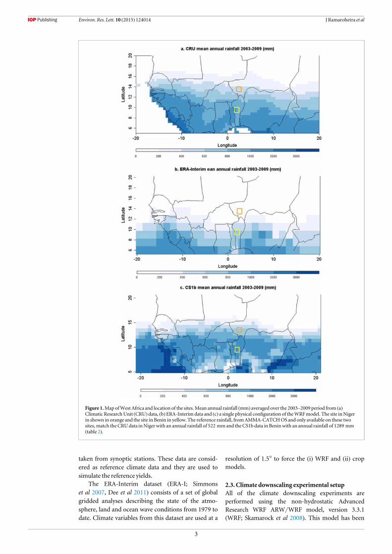
2.1. Location of the sitesTwo sites of approximately one squared-degree(figure 1) are retained for this study; they arecharacterized by a rain-fed agriculture with low inputon poor soils. The Niger site (orange box) is typical ofCentral Sahel conditions. There, the rainy seasonlasts approximately from June to September andprovides roughly 450–600 mm of rainfall. The Beninsite (yellow box) is in the Sudanian zone. There, therainy season lasts up to six months from May toOctober providing 1200–1300 mm of rainfallper year.

2.2. Climate dataFor each site, the observed meteorological data aretaken from the AMMA-CATCH observation system(African Monsoon Multidisciplinary Analysis—Cou-pling the Tropical Atmosphere and the HydrologicalCycle; www.amma-catch.org). The precipitation isinterpolated by kriging over each site using more than50 rain-gauge measurements for the 2003–2009 per-iod (for a detailed description of the method used, seeKirstetter et al 2013) while the other variables (radia-tion, temperature, relative humidity and wind) are

2

Environ. Res. Lett. 10 (2015) 124014 J Ramarohetra et al

taken from synoptic stations. These data are consid-ered as reference climate data and they are used tosimulate the reference yields.

The ERA-Interim dataset (ERA-I; Simmonset al 2007, Dee et al 2011) consists of a set of globalgridded analyses describing the state of the atmo-sphere, land and ocean wave conditions from 1979 todate. Climate variables from this dataset are used at a

resolution of 1.5° to force the (i) WRF and (ii) cropmodels.

2.3. Climate downscaling experimental setupAll of the climate downscaling experiments areperformed using the non-hydrostatic AdvancedResearch WRF ARW/WRF model, version 3.3.1(WRF; Skamarock et al 2008). This model has been

Figure 1.Map ofWest Africa and location of the sites.Mean annual rainfall (mm) averaged over the 2003–2009 period from (a)Climatic ResearchUnit (CRU)data, (b)ERA-Interim data and (c) a single physical configuration of theWRFmodel. The site inNigerin shown in orange and the site in Benin in yellow. The reference rainfall, fromAMMA-CATCHOS and only available on these twosites,match theCRUdata inNiger with an annual rainfall of 522 mmand theCS1b data in Beninwith an annual rainfall of 1289 mm(table 2).

3

Environ. Res. Lett. 10 (2015) 124014 J Ramarohetra et al

used in a large number of studies, some of which focuson West Africa (e.g. Vigaud et al 2009, Flaounaset al 2010, Klein et al 2015), and includes a large choiceof physical schemes. Simulations are carried out for adomain extending from 10° S to 30°N and 45°W to45° E, covering the large West African region, at aresolution of 80 km. Lateral forcings are provided bysix hourly ERA-I re-analyses and the integrations werecarried out between 1 January 1989 and 31 December2010 (including one year of spin-up). Only runs from2003 to 2009 have been retained to be compared withthe observedmeteorological data and to drive the cropmodels.

Although our goal is to assess both the influence ofthe physical parameterizations on the simulated yieldbias and the uncertainties linked to the choice of onescheme over another. For computational cost reasons,it was not possible to test all of the combinations.Three sets of experiments were thus designed toaddress the sensitivity to the model settings and inter-nal variability. As the agriculture of the Sudano–Sahe-lian zone is highly dependent on rainfall, we focus onparameters that have been previously identified toexert the largest influence on rainfall in Africa (Pohlet al 2011): convective and shortwave (SW) radiationschemes (Set #1), the land surface model (LSM) andland use (LU) categories (Set #2), forced versus sto-chastic components of the regional climate variability(Set#3, through one ensemble simulation). All of theother parameters are fixed: the Yonsei University pla-netary boundary layer (Hong et al 2006), WRF Single-Moment 6-Class cloud microphysics (Hong andLim 2006), the rapid radiative transfer model long-wave radiation scheme (Mlawer et al 1997) and theMonin–Obukhov surface layer. More informationabout the model settings described below is given intable 1 and in the supplementarymaterial.

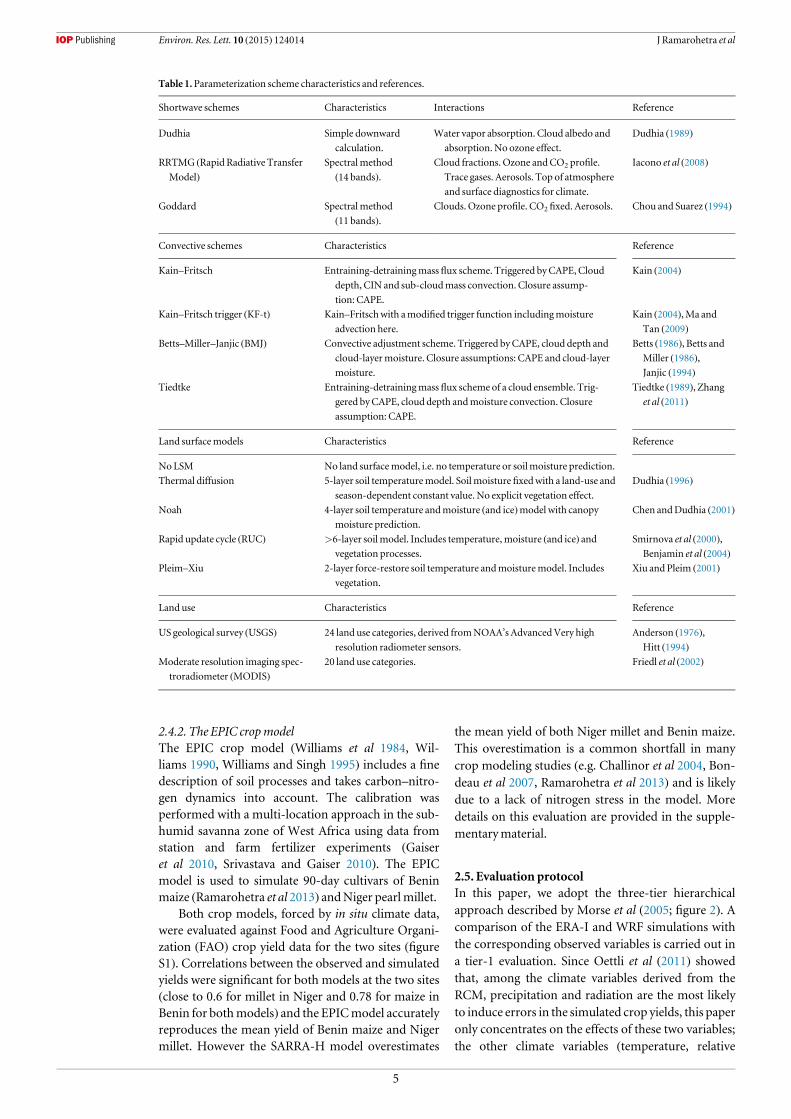
Set#1. SW radiation and atmospheric convectionSW radiation schemes can be used to estimate theamount of energy available at different altitudes, e.g.the energy of an air parcel at the surface, whileconvective parameterization schemes (CPSs) are ofprimary importance for rainfall, especially in regionsreceiving predominantly convective rainfall, as is thecase in West Africa. Set#1 addresses the sensitivity tothese two types of settings. Three SWschemes and fourCPSs are tested in this paper; theirmain characteristicsare detailed in table 1 (and the supplementarymaterial). For this set of experiments, the LSM is set tothe Noah LSM and LU is set to the USGS (UnitedStates Geological Survey) LUmap.

Set#2. LSMand LUAtmospheric models are coupled to LSMs to resolvethe fluxes at the interface between the continents andthe atmosphere. They are forced by atmospheric fieldsand use global-scale soil and surface LU datasets. LUmaps consist of typologies (e.g. 20 or 24 categories

such as agriculture, deciduous forests, grasslands,etc.), where each typology is characterized by specificalbedo, soil moisture, surface roughness and emissiv-ity values. In this set of simulations, four distinct LSMsand two LUs are tested. Due to the results inheritedfrom Set#1, the SW scheme is set to Dudhia and theCPS is set to Kain–Fritsch with the modified triggerfunction (KF-t, table 1). This is necessary in order toisolate the specific effects of the LSM and the LU data,when all other settings are constant.

Set#3. Ensemble simulationIn this Set #3, we quantify the amplitude of theuncertainties associated with the chaotic componentof the regional atmosphere in our West Africandomain (hereafter referred to as the ‘internal varia-bility’ of our model, IV). We then compare it to thechanges induced by the settingsmodified in Sets#1-2.A 10-member ensemble simulation is therefore per-formed by initializing the integrations on January 1stat 0 h UTC, and then every 6 h, thus providing 10different initial conditions. This simulation was per-formed using a unique physical configuration: theDudhia SW scheme, the KF-t CPS, the Noah LSM andtheMODIS LUdata.

2.4. Cropmodel simulationsIn order to span some of the uncertainties in cropmodeling, which have been shown to be an importantcontributor to the overall uncertainty in climateimpacts (e.g. Asseng et al 2013), we use two differentcrop models, SARRA-H and EPIC, to simulate Beninmaize yields andNiger pearlmillet yields.

2.4.1. The SARRA-H cropmodelThe SARRA-H v32 (Système d’Analyse Régionale desRisques Agroclimatiques-Habillée; http://sarra-h.teledetection.fr/SARRAH_Home.html) crop model(Dingkuhn et al 2003) was developed by CIRAD(Centre International de Recherche Agronomique).Based on a water balance model, it calculates theattainable yield under water-limited conditions bysimulating the soil water balance, potential and actualevapotranspiration, phenology, potential and water-limited assimilation, and biomass partitioning (e.g.Kouressy et al 2008, the supplementary material inSultan et al 2013). Soil nitrogen balance processes arenot simulated. The SARRA-H model is particularlysuited for the analysis of climate impacts on cerealgrowth and yield in dry tropical environments (e.g.Sultan et al 2013, Baron et al 2005, Sultan et al 2005).Trial and on-farm data were used to calibrate andvalidate the model for local varieties of Niger millet(Traoré et al 2011, Sultan et al 2013) and Benin maize(Allé et al 2014). Both varieties have a growth-cyclelength of approximately 90 days.

4

Environ. Res. Lett. 10 (2015) 124014 J Ramarohetra et al

2.4.2. The EPIC cropmodelThe EPIC crop model (Williams et al 1984, Wil-liams 1990, Williams and Singh 1995) includes a finedescription of soil processes and takes carbon–nitro-gen dynamics into account. The calibration wasperformed with a multi-location approach in the sub-humid savanna zone of West Africa using data fromstation and farm fertilizer experiments (Gaiseret al 2010, Srivastava and Gaiser 2010). The EPICmodel is used to simulate 90-day cultivars of Beninmaize (Ramarohetra et al 2013) andNiger pearlmillet.

Both crop models, forced by in situ climate data,were evaluated against Food and Agriculture Organi-zation (FAO) crop yield data for the two sites (figureS1). Correlations between the observed and simulatedyields were significant for both models at the two sites(close to 0.6 for millet in Niger and 0.78 for maize inBenin for bothmodels) and the EPICmodel accuratelyreproduces the mean yield of Benin maize and Nigermillet. However the SARRA-H model overestimates

the mean yield of both Niger millet and Benin maize.This overestimation is a common shortfall in manycrop modeling studies (e.g. Challinor et al 2004, Bon-deau et al 2007, Ramarohetra et al 2013) and is likelydue to a lack of nitrogen stress in the model. Moredetails on this evaluation are provided in the supple-mentarymaterial.

2.5. Evaluation protocolIn this paper, we adopt the three-tier hierarchicalapproach described by Morse et al (2005; figure 2). Acomparison of the ERA-I and WRF simulations withthe corresponding observed variables is carried out ina tier-1 evaluation. Since Oettli et al (2011) showedthat, among the climate variables derived from theRCM, precipitation and radiation are the most likelyto induce errors in the simulated crop yields, this paperonly concentrates on the effects of these two variables;the other climate variables (temperature, relative

Table 1.Parameterization scheme characteristics and references.

Shortwave schemes Characteristics Interactions Reference

Dudhia Simple downward

calculation.

Water vapor absorption. Cloud albedo and

absorption. No ozone effect.

Dudhia (1989)

RRTMG (Rapid Radiative TransferModel)

Spectralmethod

(14 bands).Cloud fractions.Ozone andCO2 profile.

Trace gases. Aerosols. Top of atmosphere

and surface diagnostics for climate.

Iacono et al (2008)

Goddard Spectralmethod

(11 bands).Clouds. Ozone profile. CO2fixed. Aerosols. Chou and Suarez (1994)

Convective schemes Characteristics Reference

Kain–Fritsch Entraining-detrainingmass flux scheme. Triggered byCAPE, Cloud

depth, CIN and sub-cloudmass convection. Closure assump-

tion: CAPE.

Kain (2004)

Kain–Fritsch trigger (KF-t) Kain–Fritschwith amodified trigger function includingmoisture

advection here.

Kain (2004),Ma and

Tan (2009)Betts–Miller–Janjic (BMJ) Convective adjustment scheme. Triggered byCAPE, cloud depth and

cloud-layermoisture. Closure assumptions: CAPE and cloud-layer

moisture.

Betts (1986), Betts andMiller (1986),Janjic (1994)

Tiedtke Entraining-detrainingmass flux scheme of a cloud ensemble. Trig-

gered byCAPE, cloud depth andmoisture convection. Closure

assumption: CAPE.

Tiedtke (1989), Zhanget al (2011)

Land surfacemodels Characteristics Reference

NoLSM No land surfacemodel, i.e. no temperature or soilmoisture prediction.

Thermal diffusion 5-layer soil temperaturemodel. Soilmoisture fixedwith a land-use and

season-dependent constant value.No explicit vegetation effect.

Dudhia (1996)

Noah 4-layer soil temperature andmoisture (and ice)model with canopy

moisture prediction.

Chen andDudhia (2001)

Rapid update cycle (RUC) >6-layer soilmodel. Includes temperature,moisture (and ice) andvegetation processes.

Smirnova et al (2000),Benjamin et al (2004)

Pleim–Xiu 2-layer force-restore soil temperature andmoisturemodel. Includes

vegetation.

Xiu and Pleim (2001)

Land use Characteristics Reference

US geological survey (USGS) 24 land use categories, derived fromNOAA’s AdvancedVery high

resolution radiometer sensors.

Anderson (1976),Hitt (1994)

Moderate resolution imaging spec-

troradiometer (MODIS)20 land use categories. Friedl et al (2002)

5

Environ. Res. Lett. 10 (2015) 124014 J Ramarohetra et al

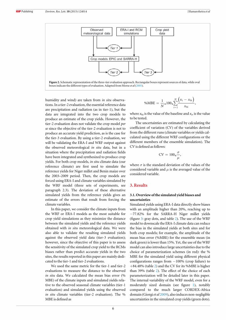
humidity and wind) are taken from in situ observa-tions. In a tier-2 evaluation, the essential reference dataare precipitation and radiation (as in tier-1), but thedata are integrated into the two crop models toproduce an estimate of the crop yields. However, thetier-2 evaluation does not validate the crop model perse since the objective of the tier-2 evaluation is not toproduce an accurate yield prediction, as is the case forthe tier-3 evaluation. By using a tier-2 evaluation, wewill be validating the ERA-I and WRF output againstthe observed meteorological in situ data, but in asituation where the precipitation and radiation fieldshave been integrated and synthesized to produce cropyields. For both crop models, in situ climate data (ourreference climate) are first used to simulate thereference yields for Niger millet and Benin maize overthe 2003–2009 period. Then, the crop models areforced using ERA-I and climate variables simulated bythe WRF model (three sets of experiments, seeparagraph 2.3). The deviation of these alternativesimulated yields from the reference yields gives anestimate of the errors that result from forcing theclimate variables.

In this paper, we consider the climate inputs fromthe WRF or ERA-I models as the most suitable forcrop yield simulations as they minimize the distancebetween the simulated yields and the reference yieldsobtained with in situ meteorological data. We werealso able to validate the resulting simulated yieldsagainst the observed yield data (tier-3 evaluation);however, since the objective of this paper is to assessthe sensitivity of the simulated crop yield to the RCMsbiases rather than predict accurate yields in the twosites, the results reported in this paper aremainly dedi-cated to the tier-1 and tier-2 evaluations.

We used the same metric for the tier-1 and tier-2evaluations to measure the distance to the observedin situ data. We calculated the mean bias error (%MBE) of the climate inputs and simulated yields rela-tive to the observed seasonal climate variables (tier-1evaluation) and simulated yields using the observedin situ climate variables (tier-2 evaluation). The %MBE is defined as

N

x x

x%MBE

1100 ,

i

N i i

i1

0

0

( )⁎ ⁎å=

-

=

where x0i is the value of the baseline and xi, is the valueto be tested.

The uncertainties are estimated by calculating thecoefficient of variation (CV) of the variables derivedfrom the different runs (climate variables or yields cal-culated using the different WRF configurations or thedifferent members of the ensemble simulation). TheCV is defined as follows:

CV 100 ,⁎sm

=

where σ is the standard deviation of the values of theconsidered variable and μ is the averaged value of theconsidered variable.

3. Results

3.1.Overview of the simulated yield biases anduncertaintiesSimulated yields using ERA-I data directly show biaseswith an amplitude higher than 20%, reaching up to−77.82% for the SARRA-H Niger millet yields(figure 3: gray dots, and table 2). The use of the WRFmodel to downscale the ERA-I climate data can reducethe bias in the simulated yields at both sites and forboth crop models; for example, the amplitude of themean bias error (%MBE) for the ensemble mean (indark green) is lower than 15%. Yet, the use of theWRFmodel can also introduce large uncertainties due to thechoice of parameterization schemes (in red): the %MBE for the simulated yield using different physicalconfigurations ranges from −100% (crop failure) to+84.48% (table 2) and the CV for its %MBE is higherthan 39% (table 2). The effect of the choice of eachparameterization will be detailed later in this paper.The internal variability of the WRF model, even for amoderately sized domain (see figure 1), notablycompared to the much larger CORDEX-Africadomain (Giorgi et al 2009), also induces non-negligibleuncertainties in the simulated crop yields (green dots).

Figure 2. Schematic representation of the three-tier evaluation approach. Rectangular boxes represent sources of data, while ovalboxes indicate the different types of evaluation. Adapted fromMorse et al (2005).

6

Environ. Res. Lett. 10 (2015) 124014 J Ramarohetra et al

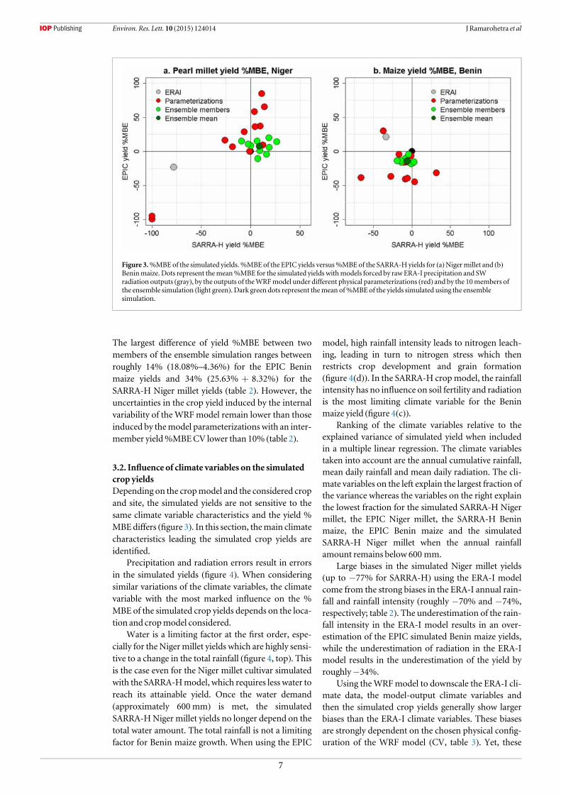
The largest difference of yield %MBE between twomembers of the ensemble simulation ranges betweenroughly 14% (18.08%–4.36%) for the EPIC Beninmaize yields and 34% (25.63%+8.32%) for theSARRA-H Niger millet yields (table 2). However, theuncertainties in the crop yield induced by the internalvariability of the WRFmodel remain lower than thoseinduced by themodel parameterizations with an inter-member yield%MBECV lower than 10% (table 2).

3.2. Influence of climate variables on the simulatedcrop yieldsDepending on the cropmodel and the considered cropand site, the simulated yields are not sensitive to thesame climate variable characteristics and the yield %MBEdiffers (figure 3). In this section, themain climatecharacteristics leading the simulated crop yields areidentified.

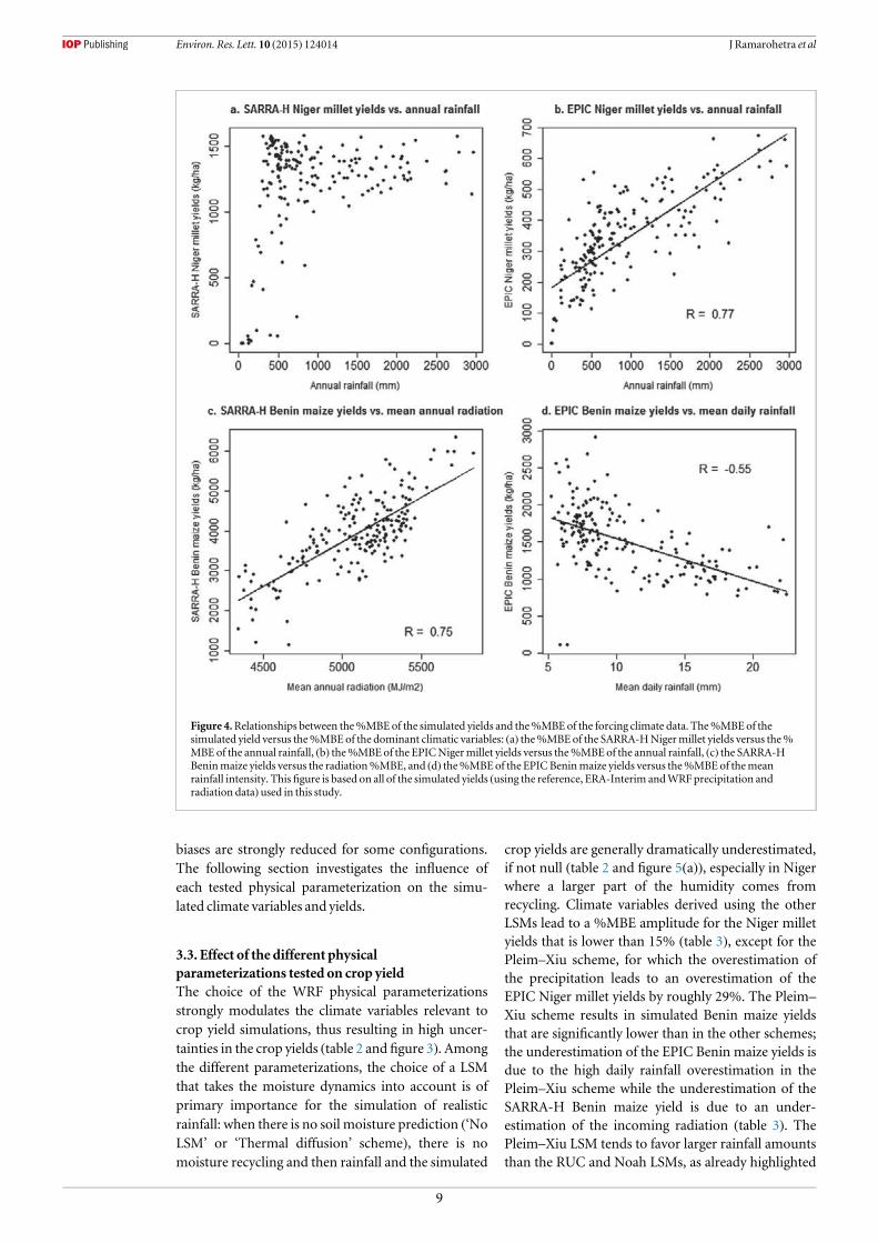
Precipitation and radiation errors result in errorsin the simulated yields (figure 4). When consideringsimilar variations of the climate variables, the climatevariable with the most marked influence on the %MBE of the simulated crop yields depends on the loca-tion and cropmodel considered.

Water is a limiting factor at the first order, espe-cially for the Nigermillet yields which are highly sensi-tive to a change in the total rainfall (figure 4, top). Thisis the case even for the Niger millet cultivar simulatedwith the SARRA-Hmodel, which requires less water toreach its attainable yield. Once the water demand(approximately 600 mm) is met, the simulatedSARRA-HNiger millet yields no longer depend on thetotal water amount. The total rainfall is not a limitingfactor for Benin maize growth. When using the EPIC

model, high rainfall intensity leads to nitrogen leach-ing, leading in turn to nitrogen stress which thenrestricts crop development and grain formation(figure 4(d)). In the SARRA-H cropmodel, the rainfallintensity has no influence on soil fertility and radiationis the most limiting climate variable for the Beninmaize yield (figure 4(c)).

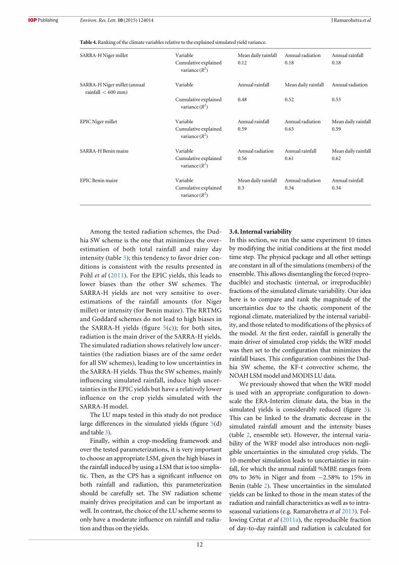
Ranking of the climate variables relative to theexplained variance of simulated yield when includedin a multiple linear regression. The climate variablestaken into account are the annual cumulative rainfall,mean daily rainfall and mean daily radiation. The cli-mate variables on the left explain the largest fraction ofthe variance whereas the variables on the right explainthe lowest fraction for the simulated SARRA-H Nigermillet, the EPIC Niger millet, the SARRA-H Beninmaize, the EPIC Benin maize and the simulatedSARRA-H Niger millet when the annual rainfallamount remains below 600mm.

Large biases in the simulated Niger millet yields(up to −77% for SARRA-H) using the ERA-I modelcome from the strong biases in the ERA-I annual rain-fall and rainfall intensity (roughly −70% and −74%,respectively; table 2). The underestimation of the rain-fall intensity in the ERA-I model results in an over-estimation of the EPIC simulated Benin maize yields,while the underestimation of radiation in the ERA-Imodel results in the underestimation of the yield byroughly−34%.

Using theWRFmodel to downscale the ERA-I cli-mate data, the model-output climate variables andthen the simulated crop yields generally show largerbiases than the ERA-I climate variables. These biasesare strongly dependent on the chosen physical config-uration of the WRF model (CV, table 3). Yet, these

Figure 3.%MBEof the simulated yields.%MBEof the EPIC yields versus%MBEof the SARRA-H yields for (a)Nigermillet and (b)Beninmaize. Dots represent themean%MBE for the simulated yields withmodels forced by rawERA-I precipitation and SWradiation outputs (gray), by the outputs of theWRFmodel under different physical parameterizations (red) and by the 10members ofthe ensemble simulation (light green). Dark green dots represent themean of%MBEof the yields simulated using the ensemblesimulation.

7

Environ. Res. Lett. 10 (2015) 124014 J Ramarohetra et al

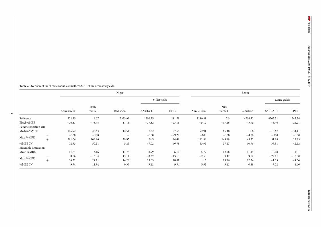
Table 2.Overview of the climate variables and the%MBEof the simulated yields.

Niger Benin

Millet yields Maize yields

Annual rain

Daily

rainfall Radiation SARRA-H EPIC Annual rain

Daily

rainfall Radiation SARRA-H EPIC

Reference 522.35 6.07 5353.99 1202.75 281.71 1289.81 7.3 4708.72 4302.51 1245.74

ERAI%MBE −70.47 −73.48 11.13 −77.82 −23.11 −5.12 −17.26 −5.95 −33.6 21.21

Parameterization sets

Median%MBE 106.92 45.63 12.51 7.22 27.54 72.91 65.48 9.6 −13.67 −34.11

Max.%MBE− −100 −100 − −100 −99.28 −100 −100 −4.68 −100 −100

+ 291.06 106.86 29.95 26.5 84.48 182.36 143.18 49.22 31.88 29.93

%MBECV 72.33 50.51 5.23 47.02 46.78 53.95 37.27 10.96 39.91 42.52

Ensemble simulation

Mean%MBE 11.64 3.16 13.75 8.99 6.19 5.77 12.08 11.15 −10.18 −14.1

Max.%MBE− 0.06 −13.34 13.14 −8.32 −13.13 −2.58 3.42 9.57 −22.11 −18.08

+ 36.22 24.71 14.29 25.63 18.87 15 19.86 12.24 −1.33 −4.36

%MBECV 9.34 11.94 0.33 9.12 9.34 5.92 5.12 0.88 7.22 4.66

8

Environ.R

es.Lett.10(2015)124014

JRam

arohetra

etal

biases are strongly reduced for some configurations.The following section investigates the influence ofeach tested physical parameterization on the simu-lated climate variables and yields.

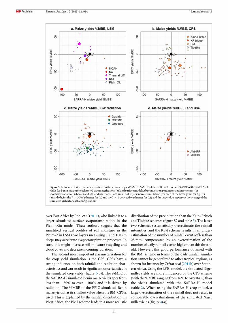
3.3. Effect of the different physicalparameterizations tested on crop yieldThe choice of the WRF physical parameterizationsstrongly modulates the climate variables relevant tocrop yield simulations, thus resulting in high uncer-tainties in the crop yields (table 2 and figure 3). Amongthe different parameterizations, the choice of a LSMthat takes the moisture dynamics into account is ofprimary importance for the simulation of realisticrainfall: when there is no soil moisture prediction (‘NoLSM’ or ‘Thermal diffusion’ scheme), there is nomoisture recycling and then rainfall and the simulated

crop yields are generally dramatically underestimated,if not null (table 2 and figure 5(a)), especially in Nigerwhere a larger part of the humidity comes fromrecycling. Climate variables derived using the otherLSMs lead to a %MBE amplitude for the Niger milletyields that is lower than 15% (table 3), except for thePleim–Xiu scheme, for which the overestimation ofthe precipitation leads to an overestimation of theEPIC Niger millet yields by roughly 29%. The Pleim–

Xiu scheme results in simulated Benin maize yieldsthat are significantly lower than in the other schemes;the underestimation of the EPIC Benin maize yields isdue to the high daily rainfall overestimation in thePleim–Xiu scheme while the underestimation of theSARRA-H Benin maize yield is due to an under-estimation of the incoming radiation (table 3). ThePleim–Xiu LSM tends to favor larger rainfall amountsthan the RUC and Noah LSMs, as already highlighted

Figure 4.Relationships between the%MBEof the simulated yields and the%MBEof the forcing climate data. The%MBEof thesimulated yield versus the%MBEof the dominant climatic variables: (a) the%MBEof the SARRA-HNigermillet yields versus the%MBEof the annual rainfall, (b) the%MBEof the EPICNigermillet yields versus the%MBEof the annual rainfall, (c) the SARRA-HBeninmaize yields versus the radiation%MBE, and (d) the%MBEof the EPICBeninmaize yields versus the%MBEof themeanrainfall intensity. Thisfigure is based on all of the simulated yields (using the reference, ERA-Interim andWRFprecipitation andradiation data) used in this study.

9

Environ. Res. Lett. 10 (2015) 124014 J Ramarohetra et al

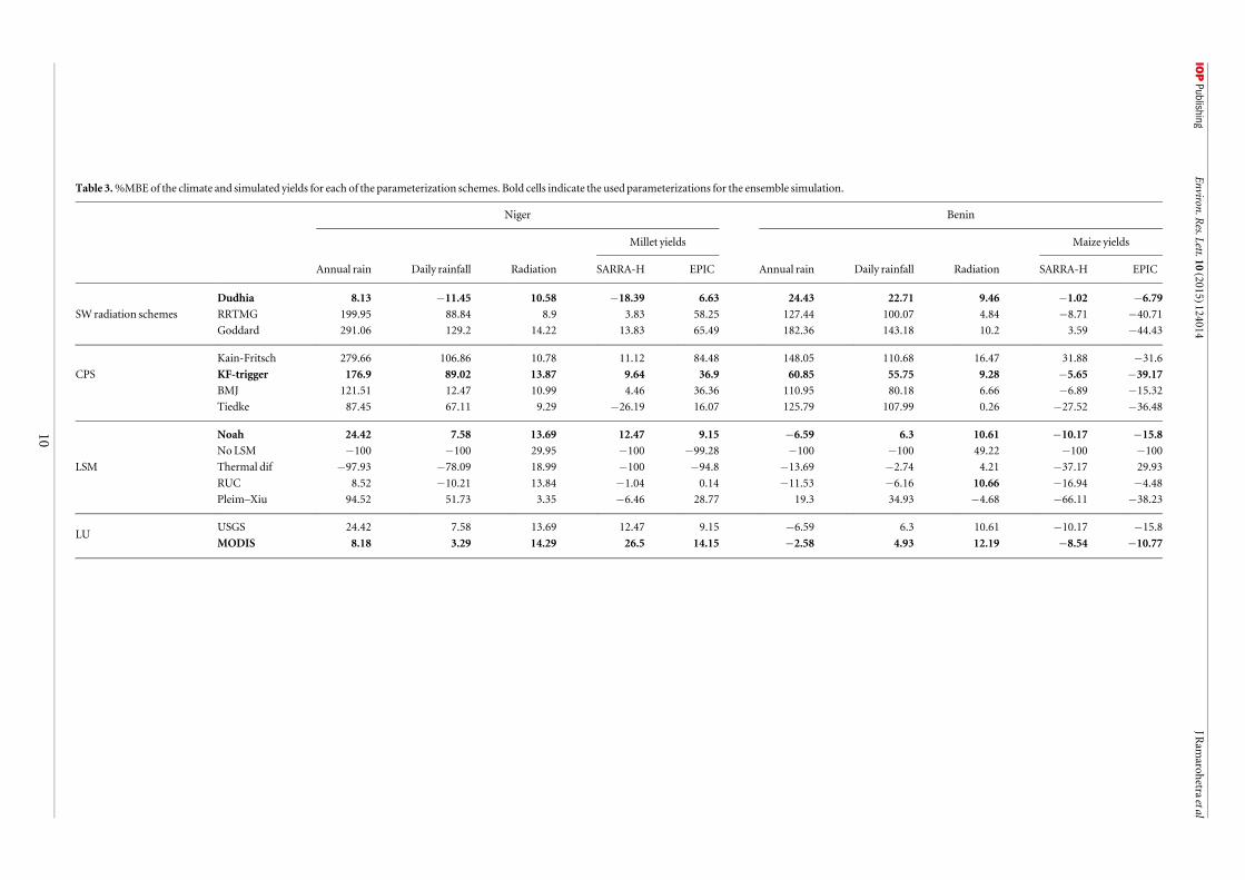
Table 3.%MBEof the climate and simulated yields for each of the parameterization schemes. Bold cells indicate the used parameterizations for the ensemble simulation.

Niger Benin

Millet yields Maize yields

Annual rain Daily rainfall Radiation SARRA-H EPIC Annual rain Daily rainfall Radiation SARRA-H EPIC

Dudhia 8.13 −11.45 10.58 −18.39 6.63 24.43 22.71 9.46 −1.02 −6.79

SW radiation schemes RRTMG 199.95 88.84 8.9 3.83 58.25 127.44 100.07 4.84 −8.71 −40.71

Goddard 291.06 129.2 14.22 13.83 65.49 182.36 143.18 10.2 3.59 −44.43

Kain-Fritsch 279.66 106.86 10.78 11.12 84.48 148.05 110.68 16.47 31.88 −31.6

CPS KF-trigger 176.9 89.02 13.87 9.64 36.9 60.85 55.75 9.28 −5.65 −39.17

BMJ 121.51 12.47 10.99 4.46 36.36 110.95 80.18 6.66 −6.89 −15.32

Tiedke 87.45 67.11 9.29 −26.19 16.07 125.79 107.99 0.26 −27.52 −36.48

Noah 24.42 7.58 13.69 12.47 9.15 −6.59 6.3 10.61 −10.17 −15.8

NoLSM −100 −100 29.95 −100 −99.28 −100 −100 49.22 −100 −100

LSM Thermal dif −97.93 −78.09 18.99 −100 −94.8 −13.69 −2.74 4.21 −37.17 29.93

RUC 8.52 −10.21 13.84 −1.04 0.14 −11.53 −6.16 10.66 −16.94 −4.48

Pleim–Xiu 94.52 51.73 3.35 −6.46 28.77 19.3 34.93 −4.68 −66.11 −38.23

LUUSGS 24.42 7.58 13.69 12.47 9.15 −6.59 6.3 10.61 −10.17 −15.8

MODIS 8.18 3.29 14.29 26.5 14.15 −2.58 4.93 12.19 −8.54 −10.77

10

Environ.R

es.Lett.10(2015)124014

JRam

arohetra

etal

over East Africa by Pohl et al (2011), who linked it to alarger simulated surface evapotranspiration in thePleim–Xiu model. These authors suggest that thesimplified vertical profiles of soil moisture in thePleim–Xiu LSM (two layers measuring 1 and 100 cmdeep)may accelerate evapotranspiration processes. Inturn, this might increase soil moisture recycling andcloud cover and decrease incoming radiation.

The second most important parameterization forthe crop yield simulation is the CPS. CPSs have astrong influence on both rainfall and radiation char-acteristics and can result in significant uncertainties inthe simulated crop yields (figure 5(b)). The %MBE ofthe SARRA-H simulated Beninmaize yields goes fromless than −50% to over +100% and it is driven byradiation. The %MBE of the EPIC simulated Beninmaize yields has its smallest value when the BMJCPS isused. This is explained by the rainfall distribution. InWest Africa, the BMJ scheme leads to a more realistic

distribution of the precipitation than the Kain–Fritschand Tiedtke schemes (figure S2 and table 3). The lattertwo schemes systematically overestimate the rainfallintensities, and the KF-t scheme results in an under-estimation of the number of rainfall events of less than25 mm, compensated by an overestimation of thenumber of daily rainfall events higher than this thresh-old. However, this good performance obtained withthe BMJ scheme in terms of the daily rainfall simula-tion cannot be generalized to other tropical regions, asshown for instance by Crétat et al (2011b) over South-ern Africa. Using the EPICmodel, the simulated Nigermillet yields are more influenced by the CPS scheme(with the%MBE ranging from 16% to over 84%) thanthe yields simulated with the SARRA-H model(table 2). When using the SARRA-H crop model, alarge overestimation of the rainfall does not result incomparable overestimations of the simulated Nigermillet yields (figure 4(a)).

Figure 5. Influence ofWRFparameterization on the simulated yield%MBE.%MBEof the EPIC yields versus%MBEof the SARRA-Hyields for Beninmaize for each tested parameterization: (a) land surfacemodels, (b) convection parameterization schemes, (c)shortwave radiation schemes and (d) land usemaps. Each small dot represents one simulation (for each of the seven years forfigures(a) and (d), for the 7×3 SW schemes for (b) and the 7×4 convective schemes for (c)) and the larger dots represent the average of thesimulated yields for each configuration.

11

Environ. Res. Lett. 10 (2015) 124014 J Ramarohetra et al

Among the tested radiation schemes, the Dud-hia SW scheme is the one that minimizes the over-estimation of both total rainfall and rainy dayintensity (table 3); this tendency to favor drier con-ditions is consistent with the results presented inPohl et al (2011). For the EPIC yields, this leads tolower biases than the other SW schemes. TheSARRA-H yields are not very sensitive to over-estimations of the rainfall amounts (for Nigermillet) or intensity (for Benin maize). The RRTMGand Goddard schemes do not lead to high biases inthe SARRA-H yields (figure 5(c)); for both sites,radiation is the main driver of the SARRA-H yields.The simulated radiation shows relatively low uncer-tainties (the radiation biases are of the same orderfor all SW schemes), leading to low uncertainties inthe SARRA-H yields. Thus the SW schemes, mainlyinfluencing simulated rainfall, induce high uncer-tainties in the EPIC yields but have a relatively lowerinfluence on the crop yields simulated with theSARRA-Hmodel.

The LU maps tested in this study do not producelarge differences in the simulated yields (figure 5(d)and table 3).

Finally, within a crop-modeling framework andover the tested parameterizations, it is very importantto choose an appropriate LSM, given the high biases inthe rainfall induced by using a LSM that is too simplis-tic. Then, as the CPS has a significant influence onboth rainfall and radiation, this parameterizationshould be carefully set. The SW radiation schememainly drives precipitation and can be important aswell. In contrast, the choice of the LU scheme seems toonly have a moderate influence on rainfall and radia-tion and thus on the yields.

3.4. Internal variabilityIn this section, we run the same experiment 10 timesby modifying the initial conditions at the first modeltime step. The physical package and all other settingsare constant in all of the simulations (members) of theensemble. This allows disentangling the forced (repro-ducible) and stochastic (internal, or irreproducible)fractions of the simulated climate variability. Our ideahere is to compare and rank the magnitude of theuncertainties due to the chaotic component of theregional climate, materialized by the internal variabil-ity, and those related tomodifications of the physics ofthe model. At the first order, rainfall is generally themain driver of simulated crop yields; the WRF modelwas then set to the configuration that minimizes therainfall biases. This configuration combines the Dud-hia SW scheme, the KF-t convective scheme, theNOAHLSMmodel andMODIS LUdata.

We previously showed that when the WRF modelis used with an appropriate configuration to down-scale the ERA-Interim climate data, the bias in thesimulated yields is considerably reduced (figure 3).This can be linked to the dramatic decrease in thesimulated rainfall amount and the intensity biases(table 2, ensemble set). However, the internal varia-bility of the WRF model also introduces non-negli-gible uncertainties in the simulated crop yields. The10-member simulation leads to uncertainties in rain-fall, for which the annual rainfall %MBE ranges from0% to 36% in Niger and from −2.58% to 15% inBenin (table 2). These uncertainties in the simulatedyields can be linked to those in the mean states of theradiation and rainfall characteristics as well as to intra-seasonal variations (e.g. Ramarohetra et al 2013). Fol-lowing Crétat et al (2011a), the reproducible fractionof day-to-day rainfall and radiation is calculated for

Table 4.Ranking of the climate variables relative to the explained simulated yield variance.

SARRA-HNigermillet Variable Mean daily rainfall Annual radiation Annual rainfall

Cumulative explained

variance (R2)0.12 0.18 0.18

SARRA-HNigermillet (annualrainfall<600 mm)

Variable Annual rainfall Mean daily rainfall Annual radiation

Cumulative explained

variance (R2)0.48 0.52 0.53

EPICNigermillet Variable Annual rainfall Annual radiation Mean daily rainfall

Cumulative explained

variance (R2)0.59 0.63 0.59

SARRA-HBeninmaize Variable Annual radiation Annual rainfall Mean daily rainfall

Cumulative explained

variance (R2)0.56 0.61 0.62

EPICBeninmaize Variable Mean daily rainfall Annual radiation Annual rainfall

Cumulative explained

variance (R2)0.3 0.34 0.34

12

Environ. Res. Lett. 10 (2015) 124014 J Ramarohetra et al

the June–July–August–September period of each yearas the ratio between V(X), the daily variance of allmembers (i.e. 122 days duplicated 10 times) andV X ,( ¯ ) the daily variance of the ensemble mean (122days): f V X

V X

( ¯ )( )

= .

On average, over the seven years, the reproduciblefraction of the day-to-day rainfall is approximately30% for both sites (29% in Niger and 31% in Benin).The inter-annual variability of these scores remainsquite low: it ranges from 21% to 35% in Niger andfrom25% to 37% inBenin. Therefore, even for amod-erate-sized domain (figure 1), the rainfall intra-seaso-nal variability is mainly driven by the stochasticcomponent of the WRF model rather than by ERA-Iforcing. Although the scores are a little higher, the day-to-day radiation variations are also strongly led by themodel’s internal variability, with averaged reproduci-bility values of 75% and 58% for the Niger and Beninsites, respectively.

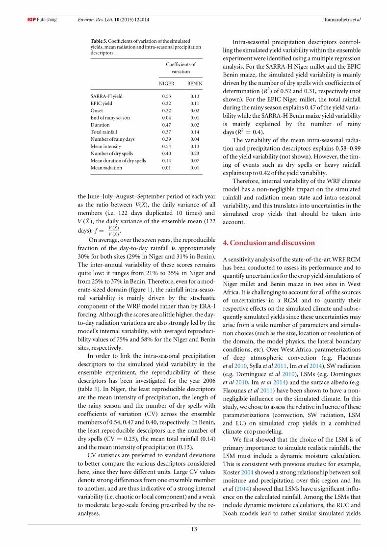
In order to link the intra-seasonal precipitationdescriptors to the simulated yield variability in theensemble experiment, the reproducibility of thesedescriptors has been investigated for the year 2006(table 5). In Niger, the least reproducible descriptorsare the mean intensity of precipitation, the length ofthe rainy season and the number of dry spells withcoefficients of variation (CV) across the ensemblemembers of 0.54, 0.47 and 0.40, respectively. In Benin,the least reproducible descriptors are the number ofdry spells (CV=0.23), the mean total rainfall (0.14)and themean intensity of precipitation (0.13).

CV statistics are preferred to standard deviationsto better compare the various descriptors consideredhere, since they have different units. Large CV valuesdenote strong differences from one ensemble memberto another, and are thus indicative of a strong internalvariability (i.e. chaotic or local component) and aweakto moderate large-scale forcing prescribed by the re-analyses.

Intra-seasonal precipitation descriptors control-ling the simulated yield variability within the ensembleexperiment were identified using amultiple regressionanalysis. For the SARRA-H Niger millet and the EPICBenin maize, the simulated yield variability is mainlydriven by the number of dry spells with coefficients ofdetermination (R2) of 0.52 and 0.31, respectively (notshown). For the EPIC Niger millet, the total rainfallduring the rainy season explains 0.47 of the yield varia-bility while the SARRA-HBeninmaize yield variabilityis mainly explained by the number of rainydays (R2=0.4).

The variability of the mean intra-seasonal radia-tion and precipitation descriptors explains 0.58–0.99of the yield variability (not shown). However, the tim-ing of events such as dry spells or heavy rainfallexplains up to 0.42 of the yield variability.

Therefore, internal variability of the WRF climatemodel has a non-negligible impact on the simulatedrainfall and radiation mean state and intra-seasonalvariability, and this translates into uncertainties in thesimulated crop yields that should be taken intoaccount.

4. Conclusion anddiscussion

A sensitivity analysis of the state-of-the-artWRF RCMhas been conducted to assess its performance and toquantify uncertainties for the crop yield simulations ofNiger millet and Benin maize in two sites in WestAfrica. It is challenging to account for all of the sourcesof uncertainties in a RCM and to quantify theirrespective effects on the simulated climate and subse-quently simulated yields since these uncertainties mayarise from a wide number of parameters and simula-tion choices (such as the size, location or resolution ofthe domain, the model physics, the lateral boundaryconditions, etc). Over West Africa, parameterizationsof deep atmospheric convection (e.g. Flaounaset al 2010, Sylla et al 2011, Im et al 2014), SW radiation(e.g. Domínguez et al 2010), LSMs (e.g. Domínguezet al 2010, Im et al 2014) and the surface albedo (e.g.Flaounas et al 2011) have been shown to have a non-negligible influence on the simulated climate. In thisstudy, we chose to assess the relative influence of theseparameterizations (convection, SW radiation, LSMand LU) on simulated crop yields in a combinedclimate-cropmodeling.

We first showed that the choice of the LSM is ofprimary importance: to simulate realistic rainfalls, theLSM must include a dynamic moisture calculation.This is consistent with previous studies: for example,Koster 2004 showed a strong relationship between soilmoisture and precipitation over this region and Imet al (2014) showed that LSMs have a significant influ-ence on the calculated rainfall. Among the LSMs thatinclude dynamic moisture calculations, the RUC andNoah models lead to rather similar simulated yields

Table 5.Coefficients of variation of the simulatedyields,mean radiation and intra-seasonal precipitationdescriptors.

Coefficients of

variation

NIGER BENIN

SARRA-H yield 0.53 0.13

EPIC yield 0.32 0.11

Onset 0.22 0.02

End of rainy season 0.04 0.01

Duration 0.47 0.02

Total rainfall 0.37 0.14

Number of rainy days 0.39 0.04

Mean intensity 0.54 0.13

Number of dry spells 0.40 0.23

Mean duration of dry spells 0.14 0.07

Mean radiation 0.01 0.01

13

Environ. Res. Lett. 10 (2015) 124014 J Ramarohetra et al

while the Pleim–Xiu LSM, driving heavier rainfall andespecially high rainfall intensities, leads to a highunderestimation of the Benin maize yields simulatedwith the EPICmodel.

Second, the convective parameterization sig-nificantly influences both rainfall and radiation.Among the tested schemes, the BMJ produces dailyrainfall intensities that are the closest to the observedintensities, and therefore it is the best scheme forBeninmaize simulations with the EPICmodel. The KFscheme is the one that overestimates the total rainfallthe most (consistent with Crétat et al 2011b, Pohlet al 2011 and Crétat and Pohl 2012), radiation andthen the simulated crop yield for both sites.

Third, the SW radiation scheme, mainly affectingrainfall, has to be chosen carefully. The Dudhiascheme produces significantly less rain than theRRTMG and Goddard schemes, thus minimizing theWRF overcompensation of the ERA-I dry bias andleading to a better crop yield estimation. The RRTMGscheme leads to slightly drier conditions than theGod-dard scheme. This is consistent with Pohl et al (2011)over East Africa.

Conversely, the tested LU model does not lead tohigh differences in the crop yields; the uncertainties inthe simulated yields are smaller than those induced bythe internal variability of the climatemodel.

In an ensemble experiment, the internal varia-bility of theWRFmodel has been shown to introducenon-negligible uncertainties in crop yield simula-tions with differences in the simulated yields reach-ing up to 30%. Dynamical downscaling can improvethe climate forcing upon re-analyses for the simula-tion of agricultural impacts at the local scale. How-ever, uncertainties arising fromboth the setting of theparameterizations and the internal variability of theRCM need to be taken into account. Adding a relaxa-tion term in the model’s prognostic equation couldallow for a more realistic timing of transient pertur-bations in the regional model, and thus favor loweruncertainties and more realistic variability at finetemporal scales. These relaxation (or nudging) tech-niques could be advisable for impact studies,although it strongly weakens the coupling betweenthe physics and dynamics of the model (Pohl andCrétat 2013).

Simulated yields have been shown in this study tobe strongly sensitive to the RCM physics and thesimulation setup. Errors and uncertainties arisingfrom such sensitivity should not be neglected. Tominimize these errors, the RCM physics must becarefully set, and to estimate uncertainties comingfrom the RCM’s internal variability, the crop modelshould be forced by an ensemble simulation of theregional climate. The use of an RCM to downscaleclimate data for crop yield simulations then implies acumbersome methodology and high-performancecomputing facilities, which calls its suitability into

question. Moreover, the choice of the best configura-tion for re-analysis downscaling does not necessarilyenable a correction of the GCMs biases (Glotteret al 2014).

Although it can probably be considered that theRCM procedure is likely to reveal its added-value inthe case of a strong resolution jumpwith theGCM for-cing or re-analyses, allowing for a more realistic reso-lution of the sub-grid processes, this may not besufficient since realistic surface boundary conditions(including topography, land-use and sub-surfaceproperties) are also needed. In this regard, due to thescarcity of high-resolution, reliable datasets doc-umenting surface and soil dynamics, climate down-scaling over Africa remains a challenging issue.

Acknowledgments

Two anonymous reviewers and one editorial boardmember are thanked for their helpful comments thathelped us improve themanuscript.WRFwas providedby the University Corporation for AtmosphericResearch website (www2.mmm.ucar.edu/wrf/users/download/). ERA-Interim data were provided by theEuropean Centre for Medium-Range Weather Fore-cast (ECMWF). WRF calculations were performedusing HPC resources from DSI-CCUB (Université deBourgogne).

References

AdamsRM,McCarl BA andMearns LO2003The effects of spatialscale of climate scenarios on economic assessments: anexample fromUS agricultureClim. Change 60 131–48

Allé C SUY, BaronC,GuibertH, Agbossou EK andAfoudaAA2014Choice and risks ofmanagement strategies ofagricultural calendar: application to themaize cultivation insouth Benin Int. J. Innov. Appl. Stud. 7 1137–47

Anderson J R 1976A land use and land cover classification systemfor use with remote sensor data (Report No. 964)ProfessionalPaperUSGovernment PrintingOffice,Washington, DC

Asseng S et al 2013Uncertainty in simulatingwheat yields underclimate changeNat. Clim. Change 3 827–32

BaronC, Sultan B, BalmeM, Sarr B, Traore S, Lebel T, Janicot S andDingkuhnM2005 FromGCMgrid cell to agricultural plot:scale issues affectingmodelling of climate impact Phil. Trans.R. Soc.B 360 2095–108

Benjamin SG,Dévényi D,Weygandt S S, BrundageK J, Brown JM,Grell GA, KimD, Schwartz B E, Smirnova TG and SmithT L2004Anhourly assimilation-forecast cycle: the RUCMon.Weather Rev. 132 495–518

Betts AK 1986Anew convective adjustment scheme. Part I:Observational and theoretical basisQ. J. R.Meteorol. Soc. 112677–91

Betts AK andMillerM J 1986Anew convective adjustment scheme.Part II: Single column tests usingGATEwave, BOMEX,ATEX and arctic air-mass data setsQ. J. R.Meteorol. Soc. 112693–709

BondeauA et al 2007Modelling the role of agriculture for the 20thcentury global terrestrial carbon balanceGlob. Change Biol.13 679–706

Challinor A J,Wheeler TR, Craufurd PQ, Slingo JM andGrimesD I F 2004Design and optimisation of a large-areaprocess-basedmodel for annual cropsAgric. For.Meteorol.124 99–120

14

Environ. Res. Lett. 10 (2015) 124014 J Ramarohetra et al

Chen F andDudhia J 2001Coupling an advanced land surface-hydrologymodel with the penn state-NCARMM5modelingsystem: I.Model implementation and sensitivityMon.Weather Rev. 129 569–85

ChouM-D and SuarezM J 1994An efficient thermal infraredradiation parameterization for use in general circulationmodelsNASATech.Memo. 104606 3 85

Crétat J,MacronC, Pohl B andRichard Y 2011aQuantifyinginternal variability in a regional climatemodel: a case studyfor SouthernAfricaClim.Dyn. 37 1335–56

Crétat J and Pohl B 2012Howphysical parameterizations canmodulate internal variability in a regional climatemodelJ. Atmos. Sci. 69 714–24

Crétat J, Pohl B, Richard Y andDrobinski P 2011bUncertainties insimulating regional climate of Southern Africa: sensitivityto physical parameterizations usingWRFClim. Dyn. 38613–34

DeeDP et al 2011The ERA-Interim reanalysis: configuration andperformance of the data assimilation systemQ. J. R.Meteorol.Soc. 137 553–97

DeryngD, SacksW J, BarfordCC andRamankuttyN2011Simulating the effects of climate and agriculturalmanagement practices on global crop yield: simulating globalcrop yieldGlob. Biogeochem. Cycles 25GB2006

Diaconescu EP, Laprise R and Sushama L 2007The impact of lateralboundary data errors on the simulated climate of a nestedregional climatemodelClim.Dyn. 28 333–50

DingkuhnM, BaronC, Bonnal V,Maraux F, Sarr B, Clopes A andForest F 2003Decision support tools for rainfed crops in theSahel at the plot and regional scalesDecision Support Tools forSmallholder Agriculture in Sub-Saharan Africa: A PracticalGuide edT E Struif Bontkes andMCSWoperis (MuscleShoals: IFDC) pp 127–39

DomínguezM,GaertnerMA, Rosnay P and de, Losada T 2010Aregional climatemodel simulation overWest Africa:parameterization tests and analysis of land-surface fieldsClim.Dyn. 35 249–65

Dudhia J 1996Amulti-layer soil temperaturemodel forMM5Preprints, The Sixth PSU/NCARMesoscaleModel Users’Workshop (Boulder, CO) pp 49–50

Dudhia J 1989Numerical study of convection observed during thewintermonsoon experiment using amesoscale two-dimensionalmodel J. Atmospheric Sci. 46 3077–107

Feser F, Rockel B, von StorchH,Winterfeldt J andZahnM2011Regional climatemodels add value to globalmodel data: areview and selected examplesBull. Am.Meteorol. Soc. 921181–92

Flaounas E, Bastin S and Janicot S 2010Regional climatemodellingof the 2006West Africanmonsoon: sensitivity to convectionand planetary boundary layer parameterisation usingWRFClim.Dyn. 36 1083–105

Flaounas E, Janicot S, Bastin S andRoca R 2011TheWest Africanmonsoon onset in 2006: sensitivity to surface albedo,orography, SST and synoptic scale dry-air intrusions usingWRFClim.Dyn. 38 685–708

FriedlMA,McIverDK,Hodges J C, ZhangXY,MuchoneyD,Strahler AH,WoodcockCE,Gopal S, SchneiderA andCooperA 2002Global land covermapping fromMODIS:algorithms and early resultsRemote Sens. Environ. 83 287–302

Gaiser T, de Barros I, Sereke F and Lange F-M2010Validation andreliability of the EPICmodel to simulatemaize production insmall-holder farming systems in tropical sub-humidWestAfrica and semi-arid BrazilAgric. Ecosyst. Environ. 135318–27

Giorgi F, Jones C andAsrarGR 2009Addressing climateinformation needs at the regional level: the CORDEXframeworkWorldMeteorol. Organ.WMOBull. 58 175

GlotterM, Elliott J,McInerneyD, BestN, Foster I andMoyer E J2014 Evaluating the utility of dynamical downscaling inagricultural impacts projections Proc. Natl Acad. Sci. USA 1118776–81

Gutmann ED, RasmussenRM, LiuC, IkedaK, GochisD J,ClarkMP,Dudhia J andThompsonG2012A comparison of

statistical and dynamical downscaling of winter precipitationover complex terrain J. Clim. 25 262–81

Hitt K J 1994Refining 1970’s land-use datawith 1990 populationdata to indicate new residential developmentWater-ResourcesInvestigations ReportNo.94-4250

Hong S-Y and Lim J-O J 2006TheWRF single-moment 6-classmicrophysics scheme (WSM6) J. KoreanMeteorol. Soc. 42129–51

Hong S-Y,NohY andDudhia J 2006Anew vertical diffusionpackagewith an explicit treatment of entrainment processesMon.Weather Rev. 134

IaconoM J, Delamere J S,Mlawer E J, ShephardMW,Clough SA andCollinsWD2008Radiative forcing by long-lived greenhouse gases: calculationswith the AER radiativetransfermodels J. Geophys. Res. Atmos. 1984–2012 113

ImE-S, Gianotti R L and Eltahir EAB 2014 Improving thesimulation of theWest Africanmonsoon using themitregional climatemodel J. Clim. 27 2209–29

Iorio J P, Duffy P B,Govindasamy B, Thompson S L,KhairoutdinovMandRandall D 2004 Effects ofmodelresolution and subgrid-scale physics on the simulation ofprecipitation in the continental United StatesClim.Dyn. 23243–58

Janjic Z I 1994The step-mountain eta coordinatemodel: furtherdevelopments of the convection, viscous sublayer, andturbulence closure schemesMon.Weather Rev. 122927–45

Jankov I, GallusWA, SegalM, ShawB andKoch S E 2005Theimpact ofDifferentWRFmodel physical parameterizationsand their interactions onwarm seasonMCS rainfallWeatherForecast. 20 1048–60

Jones JW,HoogenboomG, Porter CH, Boote K J, BatchelorWD,Hunt LA,Wilkens PW, SinghU,GijsmanA J andRitchie J T2003TheDSSAT cropping systemmodelEur. J. Agron. 18235–65

Kain J S 2004TheKain–Fritsch convective parameterization: anupdate J. Appl.Meteorol. 43 170–81

Keating BA et al 2003An overview of APSIM, amodel designed forfarming systems simulationEur. J. Agron.,ModellingCropping Syst.: Sci. Softw. Appl. 18 267–88

Kirstetter P-E, ViltardN andGossetM2013An errormodel forinstantaneous satellite rainfall estimates: evaluation ofBRAIN-TMI overWestAfr. Q. J. R.Meteorol. Soc. 139894–911

KleinC,Heinzeller D, Bliefernicht J andKunstmannH2015Variability ofWest Africanmonsoon patterns generated by aWRFmulti-physics ensembleClim. Dyn. 45 2733–5

Koster RD 2004Regions of strong coupling between soilmoistureand precipitation Science 305 1138–40

KouressyM,DingkuhnM, VaksmannMandHeinemann A B2008Adaptation to diverse semi-arid environments ofsorghum genotypes having different plant type andsensitivity to photoperiodAgric. For.Meteorol. 148357–71

KrinnerG, ViovyN, deNoblet-DucoudréN,Ogée J, Polcher J,Friedlingstein P, Ciais P, Sitch S andPrentice I C 2005Adynamic global vegetationmodel for studies of the coupledatmosphere-biosphere systemGlob. Biogeochem. Cycles 19GB1015

LeducMand Laprise R 2009Regional climatemodel sensitivity todomain sizeClim.Dyn. 32 833–54

Lobell DB andBurkeMB2010On the use of statisticalmodels topredict crop yield responses to climate changeAgric. For.Meteorol. 150 1443–52

MaL-MandTanZ-M2009 Improving the behavior of the cumulusparameterization for tropical cyclone prediction: convectiontriggerAtmos. Res. 92 190–211

Mearns LO, EasterlingW,Hays C andMarxD 2001Comparison ofagricultural impacts of climate change calculated fromhighand low resolution climate change scenarios: I. Theuncertainty due to spatial scaleClim. Change 51 131–72

Mearns LO,Mavromatis T, Tsvetsinskaya E,Hays C andEasterlingW1999Comparative responses of EPIC and

15

Environ. Res. Lett. 10 (2015) 124014 J Ramarohetra et al

CERES cropmodels to high and low spatial resolutionclimate change scenarios J. Geophys. Res. 104 6623–46

Mlawer E J, Taubman S J, BrownPD, IaconoM J andClough SA1997Radiative transfer for inhomogeneous atmospheres:RRTM, a validated correlated-kmodel for the longwaveJ. Geophys. Res. Atmos. 1984–2012 16663–82

Morse A P,Doblas-Reyes F J, HoshenMB,HagedornR andPalmer TN2005A forecast quality assessment of an end-to-end probabilisticmulti-model seasonal forecast systemusingamalariamodelTellusA 57 464–75

Oettli P, Sultan B, BaronC andVracM2011Are regional climatemodels relevant for crop yield prediction inWest Africa?Environ. Res. Lett. 6 014008

PaethH et al 2011 Progress in regional downscaling of west AfricanprecipitationAtmos. Sci. Lett. 12 75–82

Pohl B andCrétat J 2013On the use of nudging techniques forregional climatemodeling: application for tropicalconvectionClim.Dyn. 43 1693–714

Pohl B, Crétat J andCamberlin P 2011TestingWRF capability insimulating the atmospheric water cycle over Equatorial EastAfricaClim.Dyn. 37 1357–79

Ramarohetra J, Sultan B, BaronC,Gaiser T andGossetM2013Howsatellite rainfall estimate errorsmay impact rainfed cerealyield simulation inWest AfricaAgric. For.Meteorol. 180118–31

Roudier P, SultanB,Quirion P andBergA 2011The impact offuture climate change onWest African crop yields: what doesthe recent literature say?Glob. Environ. Change 21 1073–83

SethA andGiorgi F 1998The effects of domain choice on summerprecipitation simulation and sensitivity in a regional climatemodel J. Clim. 11 2698–712

ShiW, Tao F andZhang Z 2013A review on statisticalmodels foridentifying climate contributions to crop yields J. Geogr. Sci.23 567–76

SimmonsA,Uppala S, DeeD andKobayashi S 2007 ERA-Interim:NewECMWF reanalysis products from1989 onwardsECMWFNewslett. 110 25–35

SkamarockW,Klemp J B, Dudhia J, Gill D, BarkerD,DudaM,HuangX,WangWandPowers J 2008A description of theadvanced researchWRF version 3NCARTechnical NoteNCAR/TN-475+STRp 123

Smirnova TG, Brown JM, Benjamin SG andKimD2000Parameterization of cold-season processes in theMAPS land-surface scheme J. Geophys. Res. Atmos. 105 4077–86

Srivastava AK andGaiser T 2010 Simulating biomassaccumulation and yield of yam (Dioscorea alata) in theUpperOuémé Basin (Benin Republic): I. Compilation of

physiological parameters and calibration at the fieldscaleField Crops Res. 116 23–9

Sultan B, BaronC,DingkuhnM, Sarr B and Janicot S 2005Agricultural impacts of large-scale variability of theWestAfricanmonsoonAgric. For.Meteorol. 128 93–110

Sultan B, Roudier P,Quirion P, Alhassane A,Muller B,DingkuhnM,Ciais P, GuimberteauM,Traore S andBaronC2013Assessing climate change impacts on sorghum andmillet yields in the Sudanian and Sahelian savannas ofWestAfricaEnviron. Res. Lett. 8 014040

SyllaMB,Gaye AT, Pal J S, JenkinsG S andBi XQ2009High-resolution simulations ofWest African climate using regionalclimatemodel (RegCM3)with different lateral boundaryconditionsTheor. Appl. Climatol. 98 293–314

SyllaMB,Giorgi F, Ruti PM,Calmanti S andDell’Aquila A 2011The impact of deep convection on theWest African summermonsoon climate: a regional climatemodel sensitivity studyQ. J. R.Meteorol. Soc. 137 1417–30

TiedtkeM1989A comprehensivemass flux scheme for cumulusparameterization in large-scalemodelsMon.Weather Rev.117 1779–800

Traoré S B et al 2011Characterizing andmodeling the diversity ofcropping situations under climatic constraints inWest AfricaAtmos. Sci. Lett. 12 89–95

Tsvetsinskaya EA,Mearns LO,Mavromatis T, GaoW,McDaniel L andDowntonMW2003The Effect of spatialscale of climatic change scenarios on simulatedmaize, winterwheat, and rice production in the southeasternUnited StatesClim. Change 60 37–72

VigaudN, Roucou P, Fontaine B, Sijikumar S andTyteca S 2009WRF/ARPEGE-CLIMAT simulated climate trends overWest AfricaClim.Dyn. 36 925–44

Williams J R 1990 The erosion-productivity impact calculator(EPIC)model: a case history Philos. Trans. R. Soc.B 329421–8

Williams J R, Jones CA andDyke PT 1984Amodeling approach todetermining the relationship between erosion and soilproductivityTrans. ASAE 27 0129–44

Williams J R and SinghVP 1995The EPICmodelComputerModelsofWatershedHydrology pp 909–1000

XiuA and Pleim J E 2001Development of a land surfacemodel: I.Application in amesoscalemeteorologicalmodel J. Appl.Meteorol. 40 192–209

ZhangC,WangY andHamiltonK2011 Improved representation ofboundary layer clouds over the southeast Pacific in ARW-WRFusing amodifiedTiedtke cumulus parameterizationschemeMon.Weather Rev. 139 3489–513

16

Environ. Res. Lett. 10 (2015) 124014 J Ramarohetra et al

This content has been downloaded from IOPscience. Please scroll down to see the full text.

Download details:

IP Address: 91.203.34.14

This content was downloaded on 26/01/2016 at 10:06

Please note that terms and conditions apply.

Errors and uncertainties introduced by a regional climate model in climate impact

assessments: example of crop yield simulations in West Africa

View the table of contents for this issue, or go to the journal homepage for more

2015 Environ. Res. Lett. 10 124014

(http://iopscience.iop.org/1748-9326/10/12/124014)

Home Search Collections Journals About Contact us My IOPscience